Winding losses calculation for a 10 MW ironless-stator axial flux

permanent magnet generator for offshore wind power plant

Mário Matos Guerra Mesquita

Thesis for the Master of Science (MSc) Degree in

Electrical and Computer Engineering

Examination committee

Chairperson: Professor Paulo José da Costa Branco

Supervisor: Professor Joaquim António Fraga Gonçalves Dente

Members of the committee: Professor Maria José Ferreira dos Santos Lopes de Resende

November 2012

i

Acknowledgements

This thesis work has been carried out at the Department of Electric Power Engineering, Norwegian University

of Science and Technology.

I would like to express my sincere thanks and appreciation to Professor Robert Nilssen, not only for his

guidance during this research, but also for providing me with a unique opportunity of work and learning in the

field of electric machinery. In addition, special thanks are due to Engineer Zhaoqiang Zhang for his insight,

advice and patient guidance along the past months. Assistance on the access to computer servers provided by

Mr. Anders Gytri is greatly appreciated.

I wish to acknowledge Professor António Dente, not only for his constructive comments and suggestions about

this research, but also for having enlightened me with his courses on electromechanical systems at Instituto

Superior Técnico.

This master’s journey would not have been as pleasant if it was not for my colleagues. I refer not only to fellows

with whom I have been relating on a daily basis, but also to people with whom I sporadically worked to face the

challenges of complex projects.

Last but not least, my family. Words of gratitude cannot even begin to describe how thankful I am for their

constant and unconditional support.

ii

iii

Abstract

It is well-known that using expensive Litz wire is an effective solution to reduce eddy current losses in high-

speed low-power electrical machines. However, in an offshore wind power application where a direct-drive 10

MW ironless-stator generator and full-scale converter are used, the use of Litz wire becomes also necessary.

Meanwhile, the progress in the manufacture of Roebel winding and Continuously Transposed Conductors

(CTC) makes these conventional cheap solutions promising to be employed for a cost-effective generator. This

study examines the feasibility of using such technologies instead of Litz wire by studying the winding losses

associated with each solution. Completely transposed windings with different number of subconductors per turn

were considered. Both resistive and rotational losses sources are explored in this analysis by means of three-

dimensional finite element method (3-D FEM) software (i.e. Ansys Maxwell) integrated with an advanced

computing server of 48-core and 128 RAM.

In terms of resistive losses, decisive factors are the surface and length of the strand, since paths followed by

each subconductor in the interlacement process pose a small influence, especially because of the low

frequencies in play and the fact that circulating currents are highly reduced in a complete transposition. On the

other hand, rotational losses depend mainly on winding dimensions and orientation. Results show that both

proposed technologies are still far from delivering the losses reduction performance provided by Litz wire.

Keywords

Axial flux permanent magnet generator, circulating currents, continuously transposed conductors, eddy losses,

Litz wire, Roebel transposition.

iv

v

Table of Contents

Acknowledgements ................................................................................................................................................. i

Abstract.................................................................................................................................................................. iii

Table of Contents.................................................................................................................................................... v

List of Figures ....................................................................................................................................................... vii

List of Tables ......................................................................................................................................................... xi

List of Symbols .................................................................................................................................................... xiii

List of Abbreviations ............................................................................................................................................ xv

1. Introduction ........................................................................................................................................................ 1

1.1. Wind energy ................................................................................................................................................ 3

1.1.1. Offshore generator technology – state of the art .................................................................................. 4

1.2. Axial flux permanent magnet machines ...................................................................................................... 6

1.2.1. Materials and fabrication ..................................................................................................................... 9

1.2.2. Double-sided machines with a coreless stator .................................................................................... 13

1.3. Overview of the finite element method ..................................................................................................... 14

1.4. Objective of the thesis ............................................................................................................................... 15

1.5. Outline of the thesis report ........................................................................................................................ 15

2. The problem ...................................................................................................................................................... 17

2.1. Electromagnetic foundations ..................................................................................................................... 19

2.1.1. Basic field and force vectors .............................................................................................................. 19

2.1.2. Joule losses ........................................................................................................................................ 21

2.1.3. Ampère’s law ..................................................................................................................................... 23

2.1.4. Induction law ..................................................................................................................................... 24

2.1.5. Eddy currents ..................................................................................................................................... 25

2.1.6. Permanent magnets ............................................................................................................................ 26

2.2. Preponderance of current density .............................................................................................................. 28

2.3. Stator winding losses ................................................................................................................................. 29

2.3.1. Resistive losses .................................................................................................................................. 30

2.3.2. Rotational losses ................................................................................................................................ 36

2.4. The finite element method ......................................................................................................................... 39

2.5. Approach ................................................................................................................................................... 45

3. Simulation ......................................................................................................................................................... 49

3.1. Computational model of the machine........................................................................................................ 51

3.1.1. Stator winding .................................................................................................................................... 51

3.1.2. Rotor .................................................................................................................................................. 53

vi

3.2. Resistive losses .......................................................................................................................................... 54

3.2.1. Resistance .......................................................................................................................................... 55

3.2.2. Circulating currents ............................................................................................................................ 58

3.2.3. Losses results ..................................................................................................................................... 61

3.3. Rotational losses ........................................................................................................................................ 61

3.3.1. Losses results ..................................................................................................................................... 67

3.4. Algorithms................................................................................................................................................. 69

3.4.1. Central lines of transposed strands ..................................................................................................... 69

3.4.2. Arc paths forming the layers for eddy losses calculation ................................................................... 73

3.4.3. Rotational losses calculation .............................................................................................................. 75

3.4.4. Resistive losses calculation ................................................................................................................ 83

3.4.5. Flux linkage determination for circulating currents calculation ......................................................... 85

4. Conclusions ...................................................................................................................................................... 87

4.1. Main ideas ................................................................................................................................................. 89

4.2. What remains to be done ........................................................................................................................... 91

References ............................................................................................................................................................ 93

Appendix A .......................................................................................................................................................... 95

Appendix B ........................................................................................................................................................... 99

Appendix C ......................................................................................................................................................... 111

Appendix D ........................................................................................................................................................ 117

Appendix E ......................................................................................................................................................... 121

vii

List of Figures

Figure 1-1 - Topologies of RFPM machine (a) and AFPM machine (b) - Source: [4]. .......................................... 8 Figure 1-2 - Shapes of PM rotors of disc-type machines: trapezoidal (a), circular (b) and semicircular (c) -

Source: [4]. ........................................................................................................................................................... 11 Figure 1-3 - A Halbach array, showing the orientation of each piece's magnetic field. This array would give a

strong field underneath, while the field above would cancel - Source:

http://en.wikipedia.org/wiki/File:Halbach_array.png. .......................................................................................... 11 Figure 1-4 - Disc-type coreless winding assembled of coils of the same shape: (a) single coil; (b) three adjacent

coils - Source: [4]. 1 – coilside. 2 - inner offsetting bend . 3 - outer offsetting bend. .......................................... 12 Figure 1-5 - Basic topology of a double-sided AFPM machine with a coreless stator - Source: [4]. 1 – stator

winding. 2 – rotor. 3 – PM. 4 – frame. 5 – bearing. 6 – shaft. .............................................................................. 13 Figure 1-6 - Coreless winding of a three-phase, eight-pole AFPM machine with twin external rotor - Source: [4].

.............................................................................................................................................................................. 14 Figure 2-1 - Time-varying magnetic fields give rise to electric fields - Source: [6]. ............................................ 19 Figure 2-2 - Definitions of electric voltage (a) and current intensity (b) - Source: [6]. ........................................ 21 Figure 2-3 - Vectors involved in the analysis of Joule losses in a conductor - Source: [6]. ................................. 22 Figure 2-4 - Geometrical elements of Ampère’s law - Source: [6]. ...................................................................... 24 Figure 2-5 - Magnetic flux linked with a current-carrying conductor loop - Source: [6]. .................................... 24 Figure 2-6 - Magnetic coupled circuit system - Source: [6]. ................................................................................ 25 Figure 2-7 - Eddy currents in a conductor - Source: [4] - edited by author. ......................................................... 26 Figure 2-8 - Typical shape of a hysteresis loop, where HC and BR respectively denote the coercive field and the

remanence induction - Source: [6]. ....................................................................................................................... 27 Figure 2-9 - Difference in hysteresis loop of soft and hard magnetic materials - Source: [6]. ............................. 28 Figure 2-10 - Lorentz Force on one phase. 1 – rotor. 2 – PM. 3 – stator winding. v – velocity. B – magnetic

field. I – stator current. ......................................................................................................................................... 29 Figure 2-11 - Geometric configuration of the subconductors - Source: [9]. ......................................................... 30 Figure 2-12 - Subdivision of subconductor’s cross section into small rectangles - Source: [9]. .......................... 33 Figure 2-13 - Strand circuit - Source: [11] - edited by author. ............................................................................. 35 Figure 2-14 - Components of the magnetic induction vector and corresponding orientation of the eddy current

loops. .................................................................................................................................................................... 36 Figure 2-15 - Relationship between the dimensions of subconductors. ................................................................ 37 Figure 2-16 - Symmetry axis of the current density within a cross section of the conductor. .............................. 39 Figure 2-17 - Application of Ampère’s law to the current flowing threw a cylindrical conductor - Source: [6]. 46 Figure 3-1 - 2-D profile comparison between CTC and Roebel. .......................................................................... 51 Figure 3-2 - CTC with 3 strands per row 360 degrees transposed. ....................................................................... 52 Figure 3-3 - Roebel with 3 strands per row 360 degrees transposed. ................................................................... 53 Figure 3-4 - Segment of the rotor of the machine containing one pole pair. ........................................................ 53 Figure 3-5 - D465-50 hysteresis loop. .................................................................................................................. 54 Figure 3-6 - Distribution of the magnitude of current density vector at 36 Hz over the cross section of a

nonstranded conductor. ......................................................................................................................................... 55 Figure 3-7 - Distribution of the magnitude of current density vector at 36 Hz over the cross sections of a

nontransposed CTC with 2 strands per row. ......................................................................................................... 56 Figure 3-8 - Distribution of the magnitude of current density vector over a CTC with 2 strands per row. .......... 57 Figure 3-9 - Distribution of the magnitude of current density vector at 36 Hz over the cross sections of a

nontransposed Litz wire. ....................................................................................................................................... 58 Figure 3-10 - Slices and layers (orange) of a strand (green) in a CTC ................................................................. 62 Figure 3-11 - Profile and front views of the magnetic induction vector. .............................................................. 63

viii

Figure 3-12 - Volume distribution of magnetic induction vector. ........................................................................ 64 Figure 3-13 - Magnetic induction vector along selected layers of the machine. ................................................... 65 Figure 3-14 - Magnetic induction magnitude along selected layers of the machine. ............................................ 65 Figure 3-15 - From left to right: magnitude of X, Y and Z global axis components of the magnetic induction

vector. ................................................................................................................................................................... 66 Figure 3-16 - field components of layer 2. ........................................................................................................... 66 Figure 3-17 - field components of layer 10. ......................................................................................................... 67 Figure 3-18 - Total rotational losses of the machine. ........................................................................................... 68 Figure 3-19 - Total rotational losses of the machine at rated speed. ..................................................................... 68 Figure 3-20 - Length difference of two adjacent strands in the same row. ........................................................... 69 Figure 3-21 - Determination of the length difference of two adjacent strands in the same row. .......................... 70 Figure 3-22 - Fluxogram of algorithm to perform one transposition step of a CTC winding. .............................. 71 Figure 3-23 - Fluxogram of algorithm to perform a complete transposition of a Roebel winding. ...................... 72 Figure 3-24 - Fluxogram of algorithm followed to build layers used in eddy losses calculation. ........................ 74 Figure 3-25 - Fluxogram of algorithm followed to calculate eddy losses. ........................................................... 76 Figure 3-26 - Points from the central line of a massive cross section winding that form the end winding region.

.............................................................................................................................................................................. 77 Figure 3-27 - Difference in length of end region central line of each strand. ....................................................... 78 Figure 3-28 - Strand cross section: conductive layer in blue; insulation material in gray. ................................... 79 Figure 3-29 - Geometry considered for the coordinate transformations of the magnetic induction components. 80 Figure 3-30 - Coordinate transformation that takes the global X and Y components and turns each of them into

field components oriented along the winding length and width. The blue angle corresponds to G arc

x

. .............. 81

Figure 3-31 - Coordinate transformation that takes the field component oriented along the winding length and

global Z and adjusts each of them to the actual length and thickness of the segment of winding subjected to a

vertical shift. The green and yellow angles correspond to Wlength

Vshift and Wthickness

Vshift , respectively. ....................... 82

Figure 3-32 - Coordinate transformation that takes the field component oriented along the winding length and

width and adjusts each of them to the actual length and width of the segment of winding subjected to a

horizontal shift. The green and yellow angles correspond to Wwidth

Hshift and Wlength

Hshift , respectively. ....................... 83

Figure 3-33 - Fluxogram of algorithm followed to compute the impedance of each strand. ................................ 84 Figure 3-34 - Fluxogram of algorithm followed to compute flux linkage. ........................................................... 85 Figure 4-1 - Total winding losses balance. ........................................................................................................... 89 Figure B-1 - Distribution of the magnitude of current density vector at 36 Hz over the cross sections of a

nontransposed CTC with 3 strands per row. ....................................................................................................... 101 Figure B-2 - Distribution of the magnitude of current density vector over a CTC with 3 strands per row. ....... 101 Figure B-3 - Distribution of the magnitude of current density vector at 36 Hz over the cross sections of a

nontransposed CTC with 4 strands per row. ....................................................................................................... 102 Figure B-4 - Distribution of the magnitude of current density vector over a CTC with 4 strands per row. ....... 102 Figure B-5 - Distribution of the magnitude of current density vector at 36 Hz over the cross sections of a

nontransposed CTC with 5 strands per row. ....................................................................................................... 103 Figure B-6 - Distribution of the magnitude of current density vector over a CTC with 5 strands per row. ....... 104 Figure B-7 - Distribution of the magnitude of current density vector at 36 Hz over the cross sections of a

nontransposed Roebel with 2 strands per row. ................................................................................................... 105 Figure B-8 - Distribution of the magnitude of current density vector over a Roebel with 2 strands per row. .... 105 Figure B-9 - Distribution of the magnitude of current density vector at 36 Hz over the cross sections of a

nontransposed Roebel with 3 strands per row. ................................................................................................... 106 Figure B-10 - Distribution of the magnitude of current density vector over a Roebel with 3 strands per row. .. 106 Figure B-11 - Distribution of the magnitude of current density vector at 36 Hz over the cross sections of a

nontransposed Roebel with 4 strands per row. ................................................................................................... 107 Figure B-12 - Distribution of the magnitude of current density vector over a Roebel with 4 strands per row. .. 108 Figure B-13 - Distribution of the magnitude of current density vector at 36 Hz over the cross sections of a

nontransposed Roebel with 5 strands per row. ................................................................................................... 108

ix

Figure B-14 - Distribution of the magnitude of current density vector over a Roebel with 5 strands per row. .. 109 Figure C-1 - Rotational losses of a CTC with 4 strands. .................................................................................... 113 Figure C-2 - Rotational losses of a CTC with 6 strands. .................................................................................... 113 Figure C-3 - Rotational losses of a CTC with 8 strands. .................................................................................... 114 Figure C-4 - Rotational losses of a CTC with 10 strands. .................................................................................. 114 Figure C-5 - Rotational losses of a Roebel winding with 4 strands. ................................................................... 115 Figure C-6 - Rotational losses of a Roebel winding with 6 strands. ................................................................... 115 Figure C-7 - Rotational losses of a Roebel winding with 8 strands. ................................................................... 116 Figure C-8 - Rotational losses of a Roebel winding with 10 strands. ................................................................. 116 Figure E-1 - Scheme of the wooden dummy stator. ........................................................................................... 123

x

xi

List of Tables

Table 3-1 - Machine specifications. ...................................................................................................................... 51 Table 3-2 - Copper material properties. ................................................................................................................ 51 Table 3-3 - N42SH material properties. ................................................................................................................ 53 Table 3-4 - D465-50 material properties .............................................................................................................. 54 Table 3-5 - Resistance [mOhm] of the winding with a massive cross section. ..................................................... 55 Table 3-6 - Resistance [mOhm] of each strand in a non-transposed CTC winding with 2 strands per row. ........ 56 Table 3-7 - Resistance [mOhm] of each strand in a CTC winding with 2 strands per row. ................................. 56 Table 3-8 - Comparison between high and low frequency resistances. ................................................................ 57 Table 3-9 - Circulating currents at rated speed. .................................................................................................... 59 Table 3-10 - Total resistive losses. ....................................................................................................................... 61 Table 4-1 - Comparison between transpositions weighted against no transposed winding. ................................. 90 Table 4-2 - Weight of circulating currents in Joule losses. ................................................................................... 91 Table B-1 - Resistance [mOhm] of each strand in a non-transposed CTC winding with 3 strands per row. ..... 101 Table B-2 - Resistance [mOhm] of each strand in a CTC winding with 3 strands per row. ............................... 101 Table B-3 - Resistance [mOhm] of each strand in a non-transposed CTC winding with 4 strands per row. ..... 102 Table B-4 - Resistance [mOhm] of each strand in a CTC winding with 4 strands per row. ............................... 103 Table B-5 - Resistance [mOhm] of each strand in a non-transposed CTC winding with 5 strands per row. ..... 103 Table B-6 - Resistance [mOhm] of each strand in a CTC winding with 5 strands per row. ............................... 104 Table B-7 - Resistance [mOhm] of each strand in a non-transposed Roebel winding with 2 strands per row. .. 105 Table B-8 - Resistance [mOhm] of each strand in a Roebel winding with 2 strands per row. ........................... 105 Table B-9 - Resistance [mOhm] of each strand in a non-transposed Roebel winding with 3 strands per row. .. 106 Table B-10 - Resistance [mOhm] of each strand in a Roebel winding with 3 strands per row. ......................... 107 Table B-11 - Resistance [mOhm] of each strand in a non-transposed Roebel winding with 4 strands per row. 107 Table B-12 - Resistance [mOhm] of each strand in a Roebel winding with 4 strands per row. ......................... 108 Table B-13 - Resistance [mOhm] of each strand in a non-transposed Roebel winding with 5 strands per row. 109 Table B-14 - Resistance [mOhm] of each strand in a Roebel winding with 5 strands per row. ......................... 109 Table D-1 - Computational effort. ...................................................................................................................... 119

xii

xiii

List of Symbols

A Magnetic vector potential

B Magnetic induction vector

gB Normal component of magnetic flux density vector in the air gap

RB Remanence induction

C

Boundary of the method of weighted residuals

D

Electric displacement vector

E Electric field vector

condE Conduction electric field vector

gradE Gradient electric field vector

indE Induction electric field vector

F

Laplace-Lorentz force

eF

Electric force vector

mF

Magnetic force vector

pq

dkG Geometric mean distance between domain d of the

subconductor p and domain k of the subconductor q

H Magnetic field vector

CH

Coercive field

aI Armature current

J Current density vector

L

Inductance

N

Number of turns in a coil

JP Joule losses

R Electric resistance

T

Electromagnetic torque

W Weighting function

elecW

Electric energy

fldW

Stored magnetic energy

mechW

Mechanical energy

Z

Impedance matrix

ed F

Elemental electric force

eP Total rotational losses

dS Infinitesimal element of a surface

dV Infinitesimal element of a volume

dp Elemental power

dq Infinitesimal amount of free charge

dr

Infinitesimal element along length of conductor

d s Infinitesimal element of a path

f Frequency

mf Magnetic force surface density

i Current intensity

xiv

m Number of phases

cn Number of coils

Sn

Stokes’ unit normal

p

Number of pole pairs

Jp

Local power losses density

q Charge of particle

u Voltage

v

Velocity

fv

Average value of charge velocity vector parallel to the impressed

electric field originating the movement

ew Eddy losses per unit depth

eP Eddy losses

Magnetic flux

Region of the method of weighted residuals

Electric permittivity Magnetic permeability Electric resistivity

f Free charge per unit volume

Electric conductivity

Magnetic flux linkage

Angular frequency

xv

List of Abbreviations

AC Alternating Current

AFPM Axial Flux Permanent Magnet

CTC Continuously Transposed Conductors

DC Direct Current

EMF Electromotive Force

FEM Finite Element Method

MMF Magnetomotive Force

MWR Method of Weighted Residuals

PM Permanent Magnets

RFPM Radial Flux Permanent Magnet

WWEA World Wind Energy Association

xvi

1

Chapter 1

1. Introduction

In this chapter a brief description of the work is presented. Principles behind wind energy are exposed with

special emphasis being given to offshore generation. Basic structure and characteristics of AFPM machines are

described and the FEM is introduced. Objectives of the thesis are presented as well as the reasons that supported

its development. Finally, the structure of the thesis report is described.

2

3

1.1. Wind energy

“With rising costs of energy and growing concerns about the environmental effects of fossil fuel use, researchers

have been looking for alternatives as creating power sources. Wind power, a renewable and virtually

inexhaustible power source, is a promising means of green energy production. Currently, wind power is not in

wide use and accounts for the production of only about 1% of energy used world-wide. However, wind power

generation has been considerably increasing since 1999. Wind power is basically converted solar power. As the

sun heats the earth, land masses and oceans are heated in varying degrees as they absorb and reflect heat at

different rates. This causes portions of the atmosphere to warm differently and as hot air rises, atmospheric

pressure causes cooler air to replace it. The resulting movement in the air is wind. The kinetic energy of wind is

converted by turbine blades which drive a generator to produce electrical energy. Wind power can be harnessed

using wind turbines grouped together on wind farms, located either on land or offshore, for large-scale

production. Wind power generation varies in size from small generators, which produce sufficient electrical

power for a small farm, to wind farms, which can generate power for thousands of households. The intermittent

nature of wind makes reliability and storage of wind energy an important issue. Utilities must maintain

sufficient power to meet customer demand plus an additional reserve margin. Although wind is variable and at

times does not blow at all, fluctuations in the output from wind farms can be accommodated within normal

operating strategies, as the majority of wind is added to power systems as an energy source rather than a

capacity source. A spinning reserve enables a plant to meet demand. Amount of energy production is based on

the average wind speed at the site of the wind farm and the correlation between output and demand. Capacity of

wind farms also depends on geographical dispersion, i.e. the further apart wind plants are located, the greater the

chance that some of them will be producing power at any given time. The capacity of the transmission grid to

deliver wind energy to customers has been identified as one of the biggest constraints on wind energy use.

Often, high altitude windy areas, which are best suited as sites for wind farms, are not located near demand

centers, causing the power generated to be transmitted over long distances resulting in losses of power.

Moreover, costs are also increased with the necessity of building transmission lines and substations.

Environmental concern has been raised over avian fatalities caused by collisions with wind turbines. Although

bird deaths caused by wind turbines are low when compared to avian death caused by birds flying into

buildings, environmentalists insist on urging that patterns of bird flight and paths of migration should take part

into site selection for wind farms. As a result, conservationists, wind power industry officials and federal

agencies have joined together to conduct research and reduce the number of birds and bats killed by turbines.

Further environmental concerns associated with wind power include visual pollution, noise and erosion. Costs

of wind energy have dropped significantly in the last twenty years due to improvements in technology and

economies of scale - general increase in wind farm size. With wind power the energy source is free, so the costs

associated with wind energy are related to up-front costs of constructing the systems to capture energy in the

wind and convert it into electricity. Up-front capital outlays incurred by planning, purchasing of equipment,

construction of access roads and foundation and connecting to the grid and installation represent 70% of costs

associated with wind power. Maintenance, taxes, insurance and administrative costs make up the remaining

30%. Wind power is the fastest growing power source worldwide on a percentage basis and according to the

U.S. Department of Energy global winds could theoretically supply more than fifteen times current world

energy demand. Benefits of wind energy include the following” – as seen in [1]:

4

i. clean and emission free;

ii. inexhaustible and abundant;

iii. domestic resource, reducing the need to rely on foreign sources of power;

iv. growing public support;

v. cost efficient.

“One of the first wind turbines to generate electricity was a traditional wooden windmill converted by Poul la

Cour in Denmark over one hundred years ago. In the early part of the twentieth century, there were further

experimental machines but serious developments only began with the two oil shocks in the 1970s, when

governments around the world reacted by directing Research & Development money to alternatives to fuel

sources. The early 1980s saw major developments with the construction of the famous fields of hundreds of

small turbines. However, the stabilizing of the oil price in that decade and resulting reductions in the subsidies

for wind power meant that purchases from the crucial market all over the world dried up, and many wind turbine

companies withdrew from the field or went bankrupt. An exception was Denmark, where government support

meant that the knowledge base was not dissolved and the companies there were able to quickly respond when

wind energy's fortunes revived once more in the early 1990s, to the point where they and their partners continue

to have a strong position in the market today. It should be pointed out that the foundations of renewable energy's

fortunes are today based on the solid necessity of alleviating climate change and increased energy autonomy

rather than the fickle nature of oil prices. According to the World Wind Energy Association (WWEA), there was

a total global installed wind power capacity of approximately 238 GW by the end of 2011, being China the most

prominent country not only with the largest installed capacity, but also achieving an annual growth of 40%.

With the resulting economies of scale, wind energy now competes on price with the traditional generators, such

as coal and nuclear, in areas of rich wind resources” – as seen in [2].

1.1.1. Offshore generator technology – state of the art

“Offshore wind farms promise to become an important source of energy in the near future. It is expected that, by

the end of this decade, wind parks with a total capacity of thousands of megawatts will be installed in European

seas. This will be equivalent to several large traditional coal-fired power stations. Plans are currently advancing

for such large-scale wind parks in Swedish, Danish, German, Dutch, Belgian, British and Irish waters. Onshore

wind energy has grown enormously over the last decade to the point where it generates more than 10% of all

electricity in certain regions (e.g. Denmark, Schleswig-Holstein in Germany and Gotland in Sweden). However,

this expansion has not been without problems and the resistance to wind farm developments, experienced in

Britain since the mid-1990s, is now present in other countries to a lesser or greater extent. One solution of

avoiding land-use disputes and to reduce the noise and visual impacts is to move the developments offshore,

which also has a number of other advantages” – as seen in [2]:

i. availability of large continuous areas, suitable for major projects;

ii. higher wind speeds, which generally increase with distance from the shore (Britain is an exception

to this as the speed-up factor over hills means that the best wind resources are where the turbines

are also most visible);

5

iii. less turbulence, which allows the turbines to harvest the energy more effectively and reduces the

fatigue loads on the turbine;

iv. lower wind-shear (i.e. the boundary layer of slower moving wind close to the surface is thinner),

thus allowing the use of shorter towers.

But against this is the very important disadvantage of the additional capital investment necessary, relating to:

i. the more expensive marine foundations;

ii. the more expensive integration with the electrical network and, in some cases, a necessary increase

in the capacity of weak coastal grids;

iii. the more expensive installation procedures and restricted access during construction due to weather

conditions;

iv. limited access for Observations & Measurements during operation which results in an additional

penalty of reduced turbine availability and hence reduced output.

“However, the cost of wind turbines is falling and is expected to continue doing so over the coming decade.

Once sufficient experience has been gained in building offshore projects, the offshore construction industry is

likely to find similar cost-savings. At locations with good wind speeds, onshore wind energy has become a cost-

competitive resource at a stable price compared to conventional power generation, especially when

environmental benefits are accounted for. Hence, it would seem likely that offshore wind energy will also

become competitive in time. Other developments that are likely to support this trend are the design of turbines

optimized for the offshore environment, of greater sizes (i.e. up to 10 MW and over 125 meters of rotor

diameter) and with greater reliability built-in. Over the last ten and five years, the average offshore generator are

2.63 MW and 2.89 MW, respectively. At the moment, the average generator power in the wind turbines

available on the market is 3.8 MW, which implies the industry is experiencing a considerable power rating

increase [3]. With full-scale serial manufacturing generally a couple of years behind, the middle of this decade

should allow a developer to choose between several competing machines. The wind turbine manufacturing

industry has been following its own exponential growth curves over the last decade of decreasing costs by 20%,

increasing annual installed capacity by 50% and doubling the size of the largest commercially-available turbine

every three or so years. The average power rating of installed offshore wind power generator increases with a

rate of 0.25 MW per year, and will reach 4 MW after 2014 as long as the market available designs become

proven as expected [3]. The total wind power resources available offshore are vast and will certainly be able to

supply a significant proportion of electricity needs in an economic manner” – as seen in [2].

“The wind turbines being used in current offshore projects tend to be machines designed for land-use but with

modifications, such as a larger generator, a higher instrumentation specification and component redundancy,

particularly of electrical systems. If the market expands as expected, machines designed for optimized

performance offshore will be developed and utilized but it is not certain how they will look. On one hand, the

requirements from an offshore machine differ from those on land; on the other hand, the requirement for high

reliability would suggest the use of well-proven turbines. Modifications may include” – as seen in [2]:

i. larger machines, up to 5 MW or 10 MW;

6

ii. faster rotational speeds than on land, where noise restrictions generally mean that the turbine

operates slightly below optimum speed;

iii. larger generators for a specific rotor size, to enable the additionally available energy to be

efficiently harvested;

iv. high voltage generation, also possible in DC instead of AC.

“In the longer term, downwind machines with flexible blades or multiple rotors might become an option, but

engineering effort will be needed to achieve the claimed theoretical potential. The economics of offshore wind

energy encourage the development of very large wind turbines in order to justify the additional investment

necessary for the more expensive support structures, grid connection and installation procedures. The economics

will become particularly important in the deeper waters of interest to German developers and, in the longer term,

elsewhere as well, when the most suitable near-shore sites have already been developed or visual-impact

becomes an important issue” – as seen in [2].

“It would seem that the current optimism about offshore wind energy has a firm basis in currently available

technology, in likely reductions in cost and, of equal importance, in the general widespread public and political

support and the generally low impact on the environment. The experience of the first prototype offshore wind

farms has proven the technical viability and the large-scale developments currently being undertaken will bring

in much practical experience on issues such as construction methods, installation procedures, access and

Observations & Measurements philosophies, which will result in a more economic generation cost of

electricity” – as seen in [2].

Brushless permanent magnet (PM) electrical machines are the primary generators for distributed generation

systems. They are compact, high efficient and reliable self-excited generators. The distributed generation is any

electric power production technology that is integrated within a distribution system. Distributed generation

technologies are categorized as renewable and nonrenewable. Renewable technologies include solar,

photovoltaic, thermal, wind, geothermal and ocean as sources of energy. Nonrenewable technologies include

internal combustion engines, combined cycles, combustion turbines, micro turbines and fuel cells. Axial flux

permanent magnet (AFPM) brushless generators can be used both as high speed and low speed generators. Their

advantages are high power density, modular construction, high efficiency and easy integration with other

mechanical components like turbine rotors or flywheels. The output power is usually rectified and then inverted

to match the utility grid frequency or only rectified. A low speed AFPM generator is usually driven by a wind

turbine. With wind power rapidly becoming one of the most desirable alternative energy sources world-wide,

AFPM generators offer the ultimate low cost solution as compared with, for instance, solar panels [4].

1.2. Axial flux permanent magnet machines

The AFPM machine, also called the disc-type machine, is an attractive alternative to the cylindrical radial flux

permanent magnet (RFPM) machine due to its pancake shape, compact construction and high power density.

AFPM motors are particularly suitable for electrical vehicles, pumps, fans, valve control, centrifuges, machine

tools, robots and industrial equipment. AFPM machines can also operate as small to medium power generators.

Since a large number of poles can be accommodated, these machines are ideal for low speed applications, as for

7

example, electromechanical traction drives, hoists or wind generators. The unique disc-type profile of the rotor

and stator of AFPM machines makes it possible to generate diverse and interchangeable designs. AFPM

machines can be designed as single air gap or multiple air gaps machines, with slotted, slotless or even totally

ironless armature. Low power AFPM machines are frequently designed as machines with slotless windings and

surface permanent magnets [4].

The history of electrical machines reveals that the earliest machines were axial flux machines. M. Faraday’s first

primitive working prototype of an axial flux machine ever recorded, in 1831; anonymous inventor with initials

P.M., in 1832; W. Ritchie, in 1833; and B. Jacobi, in 1834. However, shortly after T. Davenport claimed the

first patent for a radial flux machine, in 1837, conventional radial flux machines have been widely accepted as

the mainstream configuration for electrical machines [4]. Several reasons arise for shelving the axial flux

machine, from the strong axial magnetic attraction force between stator and rotor, to the high costs involved in

manufacturing the laminated stator cores, whose fabrication cut is regarded as a difficult task as the assembling

of the machine itself and the requirement to keep a uniform air gap. Although the first PM excitation system was

applied to electrical machines as early as the 1830s, the poor quality of hard magnetic materials soon

discouraged their use. The invention of Alnico in 1931, barium ferrite in the 1950s and especially the rare-earth

neodymium-iron-boron (NdFeB) material, in 1983, have made a comeback of the PM excitation system

possible. It is generally believed that the availability of high energy PM materials is the main driving force for

exploitation of novel PM machine topologies and has thus revived the use of AFPM machines. Prices of rare-

earth PMs have been following a descending curve in the last decade of the twentieth century. With the

availability of more affordable PM materials, AFPM machines may play a more important role in the near future

[4].

From a construction point of view, brushless AFPM machines can be designed as single-sided or double-sided,

with or without armature slots, with or without armature core, with internal or external PM rotors, with surface

mounted or interior PMs and as single stage or multi-stage machines. In the case of double-sided configurations,

either the external stator or external rotor arrangement can be adopted. The first choice has the advantage of

using fewer PMs at the expense of poor winding utilization while the second one is considered as a particularly

advantageous machine topology. The diverse topologies of AFPM brushless machines may be classified as

follows [4]:

i. single-sided AFPM machines:

a. with slotted stator;

b. with slotless stator;

c. with salient-pole stator.

ii. double-sided AFPM machines:

a. with internal stator:

1. with slotted stator;

2. with slotless stator:

(i). with iron core stator;

(ii). with coreless stator;

(iii). without both rotor and stator cores.

8

3. with salient pole stator.

b. with internal rotor:

1. with slotted stator;

2. with slotless stator;

3. with salient pole stator.

iii. multidisc AFPM machines.

The machine studied in this research is double-sided with internal coreless stator.

The air gap of the slotted armature AFPM machine is relatively small. The mean magnetic flux density in the air

gap decreases under each slot opening due to increase in the reluctance. For AFPM machines with slotless

windings the air gap is much larger and compared to a conventional slotted winding, the slotless armature

winding has advantages such as simple stator assembly, elimination of the cogging torque (i.e. the torque due to

the interaction between the permanent magnets of the rotor and the stator slots) and reduction of rotor surface

losses, magnetic saturation and acoustic noise. The disadvantages include the use of more PM material, lower

winding inductances sometimes causing problems for inverter-fed motors and significant eddy current losses in

slotless conductors. Depending on the application and operating environment, slotless stators may have

ferromagnetic cores or be completely coreless. Coreless stator configurations eliminate any ferromagnetic

material from the armature system, thus making the associated eddy current and hysteresis core losses

nonexistent. This type of configuration also eliminates axial magnetic attraction forces between the stator and

rotor at zero-current state [4].

In pace with the application of new materials, innovation in manufacturing technology and improvements in

cooling techniques, further increase in the power density (output power per mass or volume) of the electrical

machine has been made possible [4]. There is an inherent limit to this increase for conventional RFPM machines

because of:

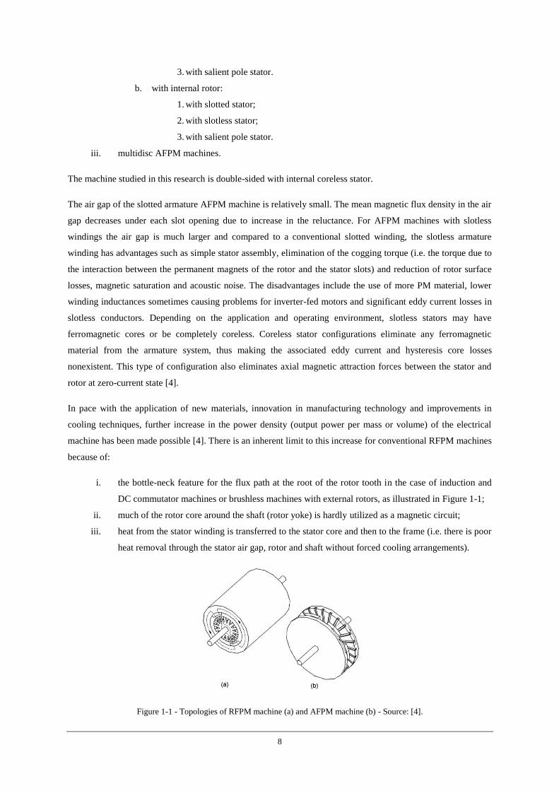
i. the bottle-neck feature for the flux path at the root of the rotor tooth in the case of induction and

DC commutator machines or brushless machines with external rotors, as illustrated in Figure 1-1;

ii. much of the rotor core around the shaft (rotor yoke) is hardly utilized as a magnetic circuit;

iii. heat from the stator winding is transferred to the stator core and then to the frame (i.e. there is poor

heat removal through the stator air gap, rotor and shaft without forced cooling arrangements).

Figure 1-1 - Topologies of RFPM machine (a) and AFPM machine (b) - Source: [4].

9

These limitations are inherently bound with radial flux structures and cannot be removed easily unless a new

topology is adopted. The AFPM machine, recognized as having a higher power density than the RFPM machine,

is more compact than its radial flux counterpart. Moreover, since the inner diameter of the core of an AFPM

machine is usually much greater than the shaft diameter, better ventilation and cooling can be expected [4]. In

general, the special properties of AFPM machines, which are considered advantageous over RFPM machines in

certain applications, can be summarized as follows:

i. AFPM machines have much larger diameter to length ratio than RFPM machines;

ii. AFPM machines have a planar and somewhat adjustable air gap;

iii. capability of being designed to possess a higher power density with some saving in core material;

iv. the topology of an AFPM machine is ideal to design a modular machine in which the number of

the same modules is adjusted to power or torque requirements;

v. the larger the outer diameter of the core, the higher the number of poles that can be accommodated,

making the AFPM machines a suitable choice for high frequency or low speed operations.

The power range of AFPM disc-type brushless machines is now from a fraction of a Watt to sub-MW. As the

output power of the AFPM machine increases, the contact surface between the rotor and shaft becomes smaller

in comparison with the rated power. It is more difficult to design a high mechanical integrity rotor-shaft joint in

the higher range of the output power. A common solution to the improvement of the mechanical integrity of the

rotor-shaft joint is to design a multidisc machine. Since the scaling of the torque capability of the AFPM

machine as the cube of the diameter while the torque of a RFPM machines scale as the square of the diameter

times the length, the benefits associated with axial flux geometries may be lost as the power level or the

geometric ratio of the length to diameter of the motor is increased. The transition occurs near the point where

the radius equals twice the length of RFPM machine. This may be a limiting design consideration for the power

rating of a single-stage disc machine as the power level can always be increased by simply stacking of disc

machines on the same shaft and in the same enclosure [4].

1.2.1. Materials and fabrication

Magnetic circuits of rotors consist of PMs and mild steel backing rings or discs. Since the air gap is somewhat

larger than that in similar RFPM counterparts, high energy density PMs should be used. Normally, surface

magnets are glued to smooth backing rings or rings with cavities of the same shape as magnets without any

additional mechanical protection against normal attractive forces. Epoxy, acrylic or silicon based adhesives are

used for gluing between magnets and backing rings or between magnets. There were attempts to develop interior

PM rotor for AFPM machines. Rotor poles can only be fabricated by using soft magnetic powders. The main

advantage of this configuration is the improved flux weakening performance. However, the complexity and high

cost of the rotor structure discourage further commercializing development.

A PM can produce magnetic flux in an air gap with no exciting winding and no dissipation of electric power. As

any other ferromagnetic material, a PM can be described by its hysteresis loop. PMs are also called hard

magnetic material, which means ferromagnetic materials with a wide hysteresis loop, as will be explained with

more detail further on this report. There are three classes of PMs currently used for electric machines:

10

i. Alnicos (Al, Ni, Co, Fe);

ii. Ceramics (ferrites), e.g. barium ferrite and strontium ferrite;

iii. Rare-earth materials, e.g. samarium-cobalt and neodymium-iron-boron.

Alnico magnets dominated the PM motor market in the range from a few watts to 150 kW between the mid-

1940s and the late 1960s. The main advantages of Alnico are its high magnetic remanent flux density and low

temperature coefficients. The temperature coefficient of remanence induction is -0.02% per degree Celsius and

maximum service temperature is 520 degrees Celsius. Unfortunately, the coercive force is very low and the

demagnetization curve is extremely non-linear. Therefore, it is very easy not only to magnetize but also to

demagnetize Alnico. Alnico has been used in PM DC commutator motors of the disc type with relatively large

air gaps. This results in a negligible armature reaction magnetic flux acting on the PMs. Sometimes, Alnico PMs

are protected from the armature flux, and consequently from demagnetization, using additional mild steel pole

shoes [4].

Barium and strontium ferrites produced by powder metallurgy were invented in the 1950s. Ferrite magnets are

available in isotropic and anisotropic grades. A ferrite has a higher coercive force than Alnico, but at the same

time has a lower remanent magnetic flux density. Temperature coefficients are relatively high, i.e. the

coefficient of remanence induction is -0.20% per degree Celsius and the coefficient of coercive field is -0.27 to -

0.4% per degree Celsius. The maximum service temperature is 450 degrees Celsius. The main advantages of

ferrites are their low cost and very high electric resistance, which means practically no eddy-current losses in the

PM volume [4].

The first generation of rare-earth permanent magnets has been commercially produced since the early 1970s. It

had the advantage of a high remanent flux density, high coercive force, high energy product, a linear

demagnetization curve and a low temperature coefficient. The temperature coefficient of remanence induction is

-0.02 to -0.045% per degree Celsius and the temperature coefficient of coercive field is -0.14 to -0.40% per

degree Celsius. Maximum service temperature is 300 to 350 degrees Celsius. It is suitable for motors with low

volumes and motors operating at increased temperatures, e.g. brushless generators for micro turbines. Elements

that make up this first generation (i.e. Sm and Co) are relatively expensive due to their supply restrictions. With

the discovery in the recent years of a second generation of rare-earth magnets on the basis of inexpensive

neodymium (Nd), remarkable progress with regard to lowering raw material costs has been achieved. The new

generation of rare-earth PMs based on inexpensive Nd was announced in 1983. The Nd is a much more

abundant rare-earth element than Sm. NdFeB magnets, which are now produced in increasing quantities have

better magnetic properties than those of SmCo, but unfortunately only at room temperature. The

demagnetization curves, especially the coercive force, are strongly temperature dependent. The temperature

coefficient of remanence induction is -0.09 to -0.15% per degree Celsius and the temperature coefficient of

coercive field is -0.40 to -0.80% per degree Celsius. The maximum service temperature is 250 degrees Celsius.

The NdFeB is also susceptible to corrosion. NdFeB magnets have great potential for considerably improving the

performance-to-cost ratio for many applications. For this reason they will have a major impact on the

development and application of PM machines in the future [4].

11

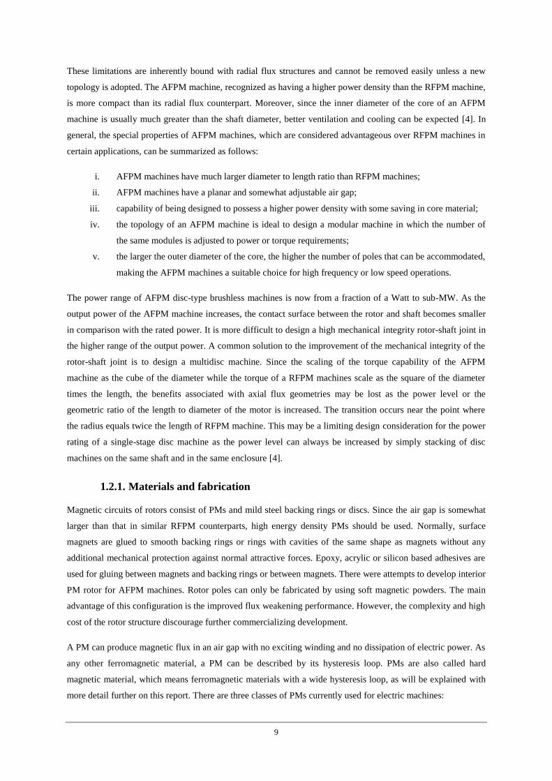
Magnetic circuits of rotors of AFPM brushless machines provide the excitation flux and are designed as PMs

glued to a ferromagnetic ring or disc which serves as a backing magnetic circuit (yoke), or PMs arranged into

Halbach array without any ferromagnetic core. Shapes of PMs are usually trapezoidal, circular or semicircular,

as illustrated in Figure 1-2. The shape of PMs affects the distribution of the air gap magnetic field and contents

of higher space harmonics. The output voltage quality (harmonic content of the generated EMF) of AFPM

generators depends on the PM geometry (circular, semicircular, trapezoidal) and distance between adjacent

magnets. Since the magnetic flux in the rotor magnetic circuit is stationary, mild steel (carbon steel) backing

rings can be used [4].

Figure 1-2 - Shapes of PM rotors of disc-type machines: trapezoidal (a), circular (b) and semicircular (c) - Source: [4].

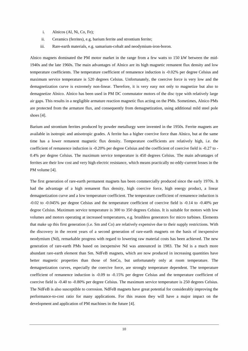
The key concept of Halbach array is that the magnetization vector of PMs should rotate as a function of distance

along the array, as exposed in Figure 1-3, providing the following advantages:

i. the fundamental field is stronger by a factor of 1.4 than in a conventional PM array, and thus the

power efficiency of the machine is doubled;

ii. the array of PMs does not require any backing steel magnetic circuit and PMs can be bonded

directly to a non-ferromagnetic supporting structure (e.g. aluminum and plastics);

iii. the magnetic field is more sinusoidal than that of a conventional PM array;

iv. Halbach array has very low back-side fields.

Figure 1-3 - A Halbach array, showing the orientation of each piece's magnetic field. This array would give a strong field

underneath, while the field above would cancel - Source: http://en.wikipedia.org/wiki/File:Halbach_array.png.

12

Armature windings of electric motors are made of solid copper conductor wires with round or rectangular cross

sections, whose conductivity is temperature dependent. The maximum temperature rise for the windings of

electrical machines is determined by the temperature limits of insulating materials. A polyester-imide and

polyamide-imide coat can provide an operating temperature of 200 degrees Celsius. The highest operating

temperatures (over 600 degrees Celsius) can be achieved using nickel clad copper or palladium-silver conductor

wires and ceramic insulation [4].

Stator coreless windings of AFPM machines are fabricated as uniformly distributed coils on a disc-type

cylindrical supporting structure (hub) made of nonmagnetic and nonconductive material. There are two types of

windings:

i. winding comprised of multi-turn coils wound with turns of insulated conductor of round or

rectangular cross section;

ii. printed winding also called film coil winding.

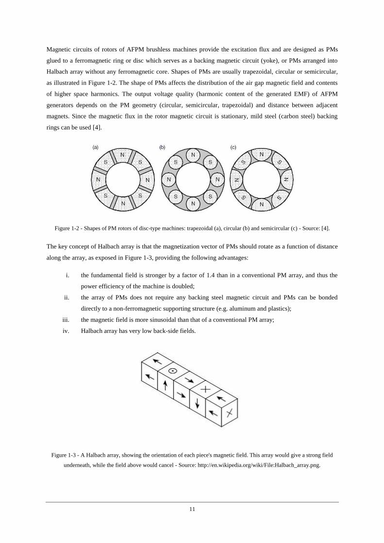
Coils are connected in groups to form the phase windings typically connected in star or delta. Coils or groups of

coils of the same phase can be connected in parallel to form parallel paths. To assemble the winding of the same

coils and obtain high density packing, coils should be formed with offsetting bends, as shown in Figure 1-4. The

space between two sides of the same coil is filled with coil sides from each of the adjacent coils [4].

Figure 1-4 - Disc-type coreless winding assembled of coils of the same shape: (a) single coil; (b) three adjacent coils -

Source: [4]. 1 – coilside. 2 - inner offsetting bend . 3 - outer offsetting bend.

Coils can be placed in a slotted structure of the mold. With all the coils in position, the winding (often with a

supporting structure or hub) is molded into a mixture of epoxy resin and hardener and then cured in a heated

oven. Because of the difficulty of releasing the cured stator from the slotted structure of the mold, each spacing

block that forms a guide slot consists of several removable pins of different size. For very small AFPM

machines and micro machines printed circuit coreless windings allow for automation of production. Printed

circuit windings for AFPM brushless machines fabricated in a similar way as printed circuit boards have not

been commercialized due to poor performance. A better performance has been achieved using film coil

windings made through the same process as flexible printed circuits. The coil pattern is formed by etching two

copper films that are then attached to both sides of a board made of insulating materials. Compact coil patterns

are made possible by connecting both sides of coil patterns through holes [4].

13

1.2.2. Double-sided machines with a coreless stator

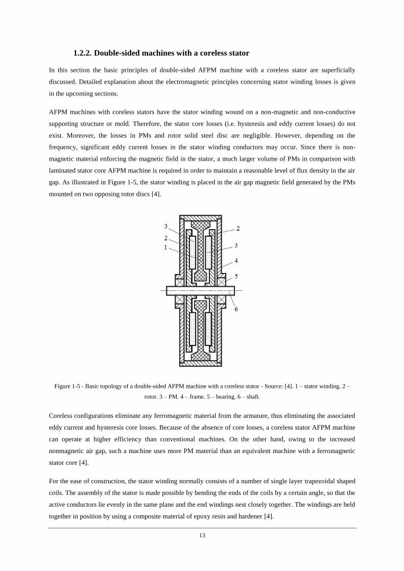
In this section the basic principles of double-sided AFPM machine with a coreless stator are superficially

discussed. Detailed explanation about the electromagnetic principles concerning stator winding losses is given

in the upcoming sections.

AFPM machines with coreless stators have the stator winding wound on a non-magnetic and non-conductive

supporting structure or mold. Therefore, the stator core losses (i.e. hysteresis and eddy current losses) do not

exist. Moreover, the losses in PMs and rotor solid steel disc are negligible. However, depending on the

frequency, significant eddy current losses in the stator winding conductors may occur. Since there is non-

magnetic material enforcing the magnetic field in the stator, a much larger volume of PMs in comparison with

laminated stator core AFPM machine is required in order to maintain a reasonable level of flux density in the air

gap. As illustrated in Figure 1-5, the stator winding is placed in the air gap magnetic field generated by the PMs

mounted on two opposing rotor discs [4].

Figure 1-5 - Basic topology of a double-sided AFPM machine with a coreless stator - Source: [4]. 1 – stator winding. 2 –

rotor. 3 – PM. 4 – frame. 5 – bearing. 6 – shaft.

Coreless configurations eliminate any ferromagnetic material from the armature, thus eliminating the associated

eddy current and hysteresis core losses. Because of the absence of core losses, a coreless stator AFPM machine

can operate at higher efficiency than conventional machines. On the other hand, owing to the increased

nonmagnetic air gap, such a machine uses more PM material than an equivalent machine with a ferromagnetic

stator core [4].

For the ease of construction, the stator winding normally consists of a number of single layer trapezoidal shaped

coils. The assembly of the stator is made possible by bending the ends of the coils by a certain angle, so that the

active conductors lie evenly in the same plane and the end windings nest closely together. The windings are held

together in position by using a composite material of epoxy resin and hardener [4].

14

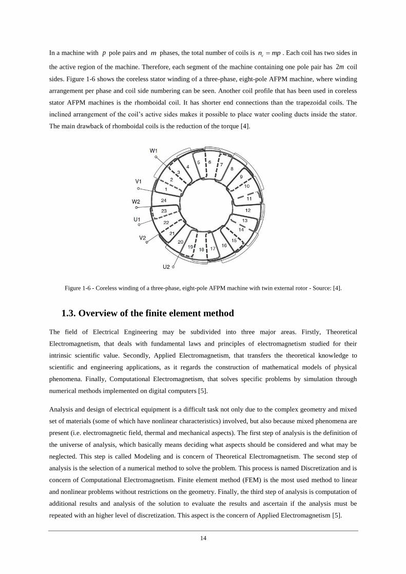
In a machine with p pole pairs and m phases, the total number of coils is cn mp . Each coil has two sides in

the active region of the machine. Therefore, each segment of the machine containing one pole pair has 2m coil

sides. Figure 1-6 shows the coreless stator winding of a three-phase, eight-pole AFPM machine, where winding

arrangement per phase and coil side numbering can be seen. Another coil profile that has been used in coreless

stator AFPM machines is the rhomboidal coil. It has shorter end connections than the trapezoidal coils. The

inclined arrangement of the coil’s active sides makes it possible to place water cooling ducts inside the stator.

The main drawback of rhomboidal coils is the reduction of the torque [4].

Figure 1-6 - Coreless winding of a three-phase, eight-pole AFPM machine with twin external rotor - Source: [4].

1.3. Overview of the finite element method

The field of Electrical Engineering may be subdivided into three major areas. Firstly, Theoretical

Electromagnetism, that deals with fundamental laws and principles of electromagnetism studied for their

intrinsic scientific value. Secondly, Applied Electromagnetism, that transfers the theoretical knowledge to

scientific and engineering applications, as it regards the construction of mathematical models of physical

phenomena. Finally, Computational Electromagnetism, that solves specific problems by simulation through

numerical methods implemented on digital computers [5].

Analysis and design of electrical equipment is a difficult task not only due to the complex geometry and mixed

set of materials (some of which have nonlinear characteristics) involved, but also because mixed phenomena are

present (i.e. electromagnetic field, thermal and mechanical aspects). The first step of analysis is the definition of

the universe of analysis, which basically means deciding what aspects should be considered and what may be

neglected. This step is called Modeling and is concern of Theoretical Electromagnetism. The second step of

analysis is the selection of a numerical method to solve the problem. This process is named Discretization and is

concern of Computational Electromagnetism. Finite element method (FEM) is the most used method to linear

and nonlinear problems without restrictions on the geometry. Finally, the third step of analysis is computation of

additional results and analysis of the solution to evaluate the results and ascertain if the analysis must be

repeated with an higher level of discretization. This aspect is the concern of Applied Electromagnetism [5].

15

In essence, the finite element is a mathematical method for solving ordinary and partial differential equations.

Since it is a numerical method, it has the ability to solve complex problems that can be represented in

differential equation form. As these types of equations occur naturally in virtually all fields of the physical

sciences, the applications of the finite element method are limitless as regards to the solution of practical design

problems. Due to the high cost of computing power of past years, FEM has a history of being used to solve

complex and cost critical problems. Classical methods alone usually cannot provide adequate information to

determine, for instance, the safe working limits of a major civil engineering construction. If a tall building, a

large suspension bridge or a nuclear reactor failed catastrophically, the economy and social costs would be

unacceptably high. In recent years, FEM has been used almost universally to solve structural engineering

problems. Nowadays, even the most simple of products rely on FEM for design evaluation, because

contemporary design problems usually cannot be solved as accurately and cheaply using any other method

currently available. Physical testing was the norm in years gone by, but now it is simply too expensive. Many

kinds of electromagnetic phenomenon can be modeled, from the propagation of microwaves to the torque in an

electromagnetic motor. Analysis of electromagnetic field passing through and around a structure provides

insight into the response and hence a means for regulating these fields to attain specific responses [5].

1.4. Objective of the thesis

The main objective of the thesis work presented in this report is to compare the losses performance of CTC and

Roebel winding when working in the coreless stator of a double-sided AFPM machine. The idea is to examine

the feasibility of using such technologies instead of the more expensive Litz wire solution. This study focuses on

comparing the two mentioned windings in terms of rotational and Joule losses, considering all aspects inherent

to a transposed coil, including circulating currents between parallel subconductors. Dimension independent

scripts to build each of the Maxwell models necessary to calculate losses parameters were developed using

Matlab.

1.5. Outline of the thesis report

The structure of this thesis follows the work evolution from basic analytical study to the complex computational

models. Thus, in this first chapter, a brief description of the work is presented. Principles behind wind energy

are exposed with special emphasis being given to offshore generation. Basic structure and characteristics of

AFPM machines are described and the FEM is introduced. The second chapter presents a brief overview on

electromagnetic foundations, moving from the most general axioms to the specificities of a double-sided

coreless stator AFPM machine, moving from there to the phenomena linked with stator winding losses. The

third chapter describes in detail the computational methods used to calculate stator winding losses. Firstly, the

three-dimensional model of the segment used to study the machine is presented, with special emphasis being

given to the architecture of the two transposed winding technologies under analysis. Results for resistive and

rotational losses are presented and the critical aspects behind the methods’ algorithms discussed. Finally, the

fourth chapter is aimed at detailing overall conclusions of the thesis as well as presenting future work

perspectives.

16

17

Chapter 2

2. The problem

To understand the principles behind any electrical machine, it is crucial to have a solid background on

electromagnetic foundations. In this chapter a brief overview on that field is provided, moving from the most

general axioms to the specificities of a double-sided coreless stator AFPM machine, moving from there to the

phenomena linked with stator winding losses. Finally, a general analytical example on the FEM is given and the

computational approach chosen to solve the proposed task is described.

18

19

2.1. Electromagnetic foundations

To understand the concepts under analysis in this report, basic knowledge of magnetic and electric field theory

is necessary. The general concepts here introduced refer to the physics behind electromagnetic rotating

machinery, by means of which the bulk of energy conversion takes place. They are constantly utilized

throughout the rest of this report. The geometric algebra formulations needed to understand the concepts from

now on described can be found in Appendix A.

2.1.1. Basic field and force vectors

From the set of Maxwell’s equations, the following is of the most importance in this analysis.

B

Et

(2.1)

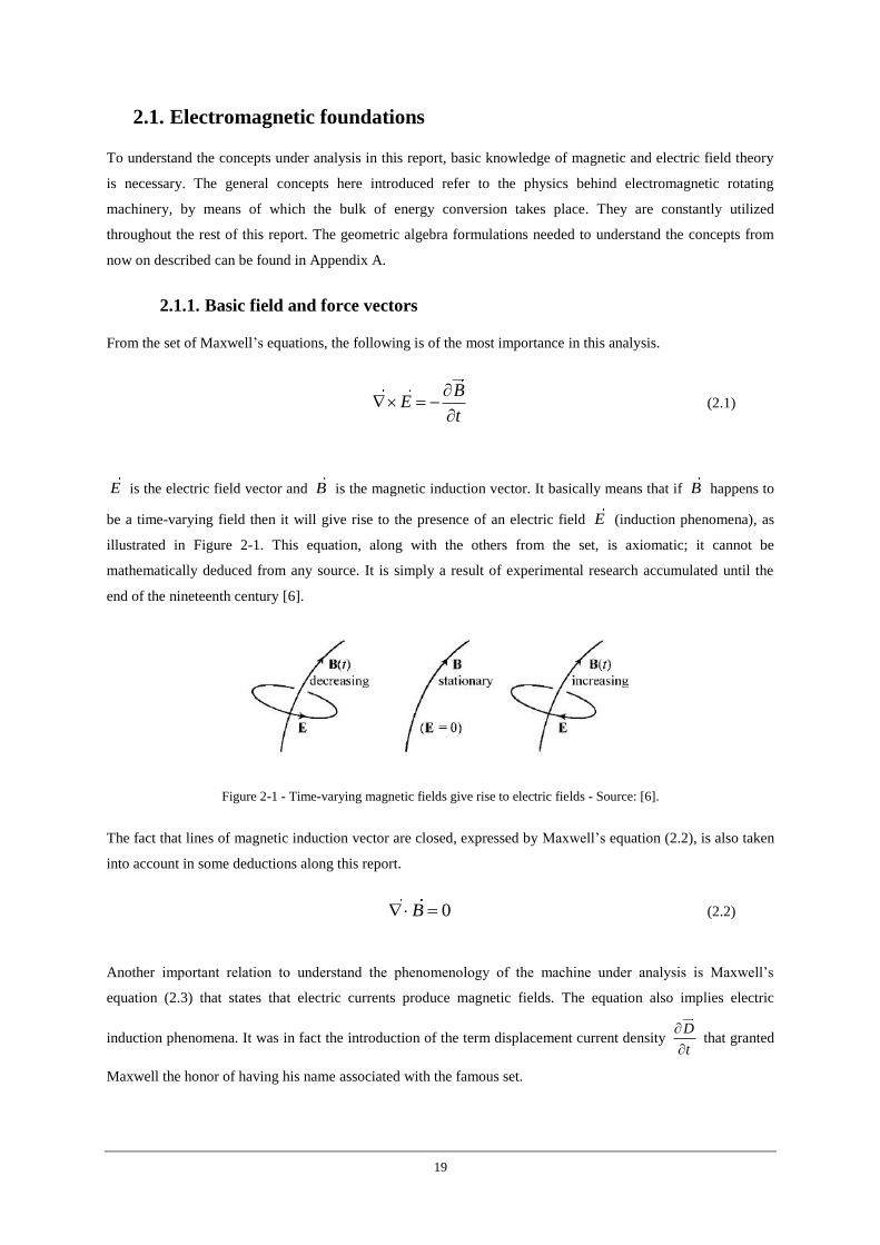
E is the electric field vector and B is the magnetic induction vector. It basically means that if B happens to

be a time-varying field then it will give rise to the presence of an electric field E (induction phenomena), as

illustrated in Figure 2-1. This equation, along with the others from the set, is axiomatic; it cannot be

mathematically deduced from any source. It is simply a result of experimental research accumulated until the

end of the nineteenth century [6].

Figure 2-1 - Time-varying magnetic fields give rise to electric fields - Source: [6].

The fact that lines of magnetic induction vector are closed, expressed by Maxwell’s equation (2.2), is also taken

into account in some deductions along this report.

0B (2.2)

Another important relation to understand the phenomenology of the machine under analysis is Maxwell’s

equation (2.3) that states that electric currents produce magnetic fields. The equation also implies electric

induction phenomena. It was in fact the introduction of the term displacement current density D

t

that granted

Maxwell the honor of having his name associated with the famous set.

20

D

H Jt

(2.3)

H is the magnetic field vector that relates with the magnetic induction vector by B H where is the

magnetic permeability of the medium. D is the electric displacement vector related to the electric field vector

by D E where is the electric permittivity of the medium.

Electromagnetic fields cannot be created from a void. Their existence requires the presence of sources, namely

charges, either at rest or moving in space. Moving charges (i.e. when currents are present) are characterized by a

current density vector J , that relates with the electric field vector by the electric conductivity , as shown in

equation (2.4).

J E (2.4)

A possible physical interpretation for the current density vector is expressed in equation (2.5).

f fJ v (2.5)

f represents the free charge per unit volume, while fv denotes the average value of the charge velocity

parallel to the impressed electric field originating the movement.

Placing a static q charged particle in a region where an electric field E is present will cause a force eF to be

exerted on the charge, as shown in equation (2.6).

eF qE (2.6)

If the same charged particle is moving with velocity v in a region where a magnetic induction field B exists, a

force mF arises according to equation (2.7).

mF q v B (2.7)

Naturally, if a moving charged particle is submitted to an electromagnetic field, the two forces will add up,

causing the so-called Laplace-Lorentz force expressed below.

F q E v B (2.8)

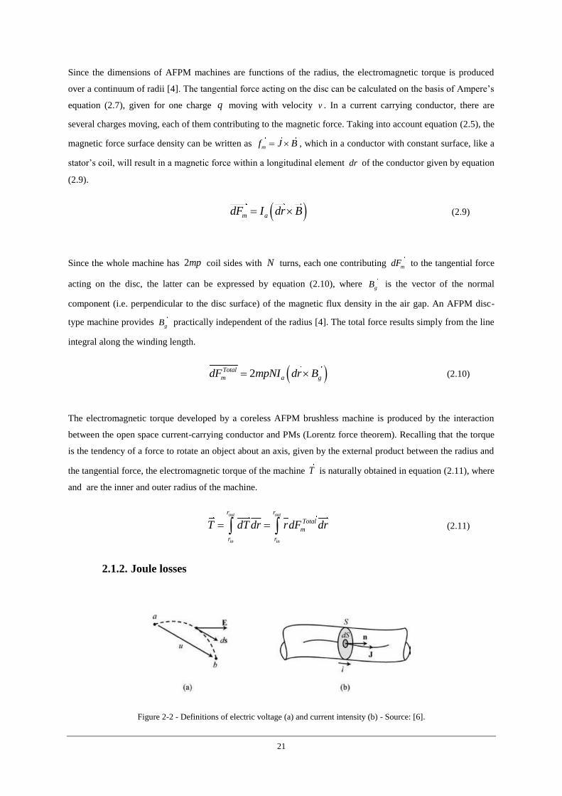
21

Since the dimensions of AFPM machines are functions of the radius, the electromagnetic torque is produced

over a continuum of radii [4]. The tangential force acting on the disc can be calculated on the basis of Ampere’s

equation (2.7), given for one charge q moving with velocity v . In a current carrying conductor, there are

several charges moving, each of them contributing to the magnetic force. Taking into account equation (2.5), the

magnetic force surface density can be written as mf J B , which in a conductor with constant surface, like a

stator’s coil, will result in a magnetic force within a longitudinal element dr of the conductor given by equation

(2.9).

m adF I dr B (2.9)

Since the whole machine has 2mp coil sides with N turns, each one contributing mdF to the tangential force

acting on the disc, the latter can be expressed by equation (2.10), where gB is the vector of the normal

component (i.e. perpendicular to the disc surface) of the magnetic flux density in the air gap. An AFPM disc-

type machine provides gB practically independent of the radius [4]. The total force results simply from the line

integral along the winding length.

2Total

m a gdF mpNI dr B (2.10)

The electromagnetic torque developed by a coreless AFPM brushless machine is produced by the interaction

between the open space current-carrying conductor and PMs (Lorentz force theorem). Recalling that the torque

is the tendency of a force to rotate an object about an axis, given by the external product between the radius and

the tangential force, the electromagnetic torque of the machine T is naturally obtained in equation (2.11), where

and are the inner and outer radius of the machine.

out out

in in

r r

Total

m

r r

T dT dr rdF dr (2.11)

2.1.2. Joule losses

Figure 2-2 - Definitions of electric voltage (a) and current intensity (b) - Source: [6].

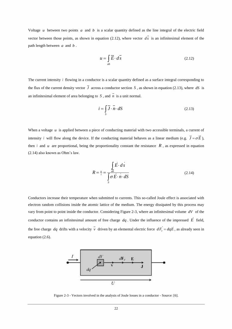
22

Voltage u between two points a and b is a scalar quantity defined as the line integral of the electric field

vector between those points, as shown in equation (2.12), where vector d s is an infinitesimal element of the

path length between a and b .

ab

u E d s (2.12)

The current intensity i flowing in a conductor is a scalar quantity defined as a surface integral corresponding to

the flux of the current density vector J across a conductor section S , as shown in equation (2.13), where dS is

an infinitesimal element of area belonging to S , and n is a unit normal.

S

i J n dS (2.13)

When a voltage u is applied between a piece of conducting material with two accessible terminals, a current of

intensity i will flow along the device. If the conducting material behaves as a linear medium (e.g. J E ),

then i and u are proportional, being the proportionality constant the resistance R , as expressed in equation

(2.14) also known as Ohm’s law.

abu

i

S

E d s

RE n dS

(2.14)

Conductors increase their temperature when submitted to currents. This so-called Joule effect is associated with

electron random collisions inside the atomic lattice of the medium. The energy dissipated by this process may

vary from point to point inside the conductor. Considering Figure 2-3, where an infinitesimal volume dV of the

conductor contains an infinitesimal amount of free charge dq . Under the influence of the impressed E field,

the free charge dq drifts with a velocity v driven by an elemental electric force ed F dqE , as already seen in

equation (2.6).

Figure 2-3 - Vectors involved in the analysis of Joule losses in a conductor - Source: [6].

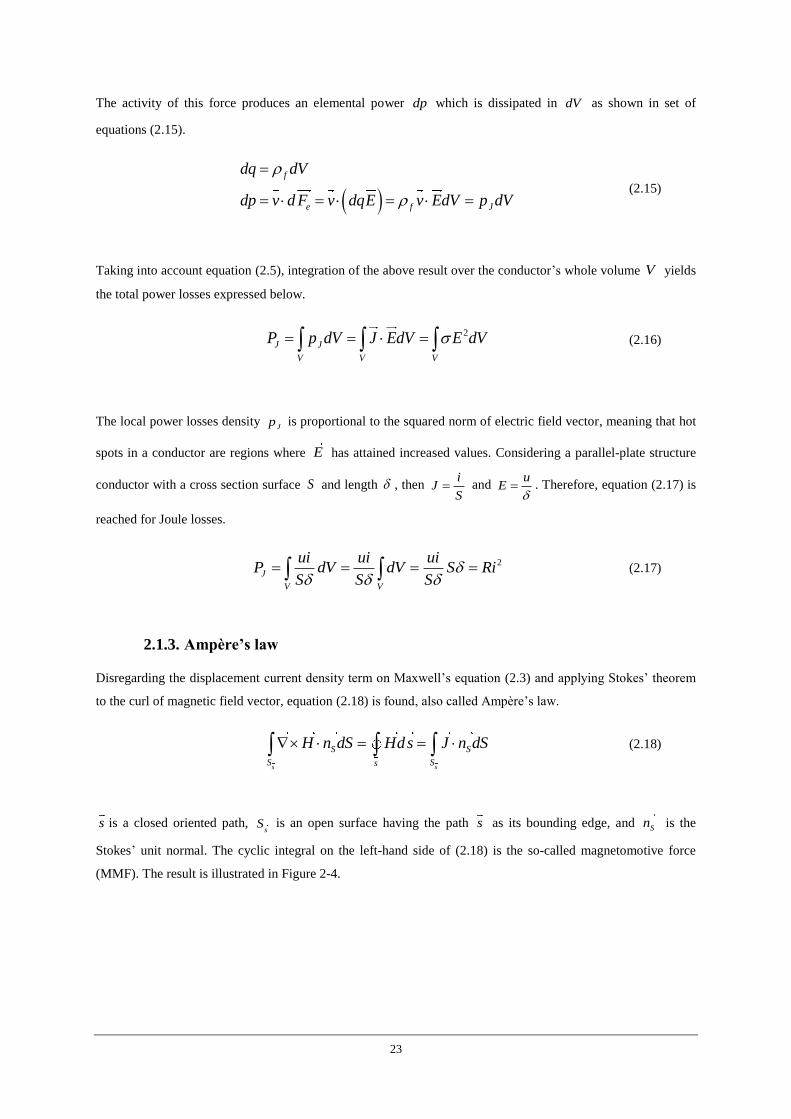
23

The activity of this force produces an elemental power dp which is dissipated in dV as shown in set of

equations (2.15).

f

e f J

dq dV

dp v d F v dqE v EdV p dV

(2.15)

Taking into account equation (2.5), integration of the above result over the conductor’s whole volume V yields

the total power losses expressed below.

2

J J

V V V

P p dV J EdV E dV (2.16)

The local power losses density Jp is proportional to the squared norm of electric field vector, meaning that hot

spots in a conductor are regions where E has attained increased values. Considering a parallel-plate structure

conductor with a cross section surface S and length , then i

JS

and u

E

. Therefore, equation (2.17) is

reached for Joule losses.

2

J

V V

ui ui uiP dV dV S Ri

S S S

(2.17)

2.1.3. Ampère’s law

Disregarding the displacement current density term on Maxwell’s equation (2.3) and applying Stokes’ theorem

to the curl of magnetic field vector, equation (2.18) is found, also called Ampère’s law.

s s

S S

S Ss

H n dS Hds J n dS (2.18)

s is a closed oriented path, s

S is an open surface having the path s as its bounding edge, and Sn is the

Stokes’ unit normal. The cyclic integral on the left-hand side of (2.18) is the so-called magnetomotive force

(MMF). The result is illustrated in Figure 2-4.

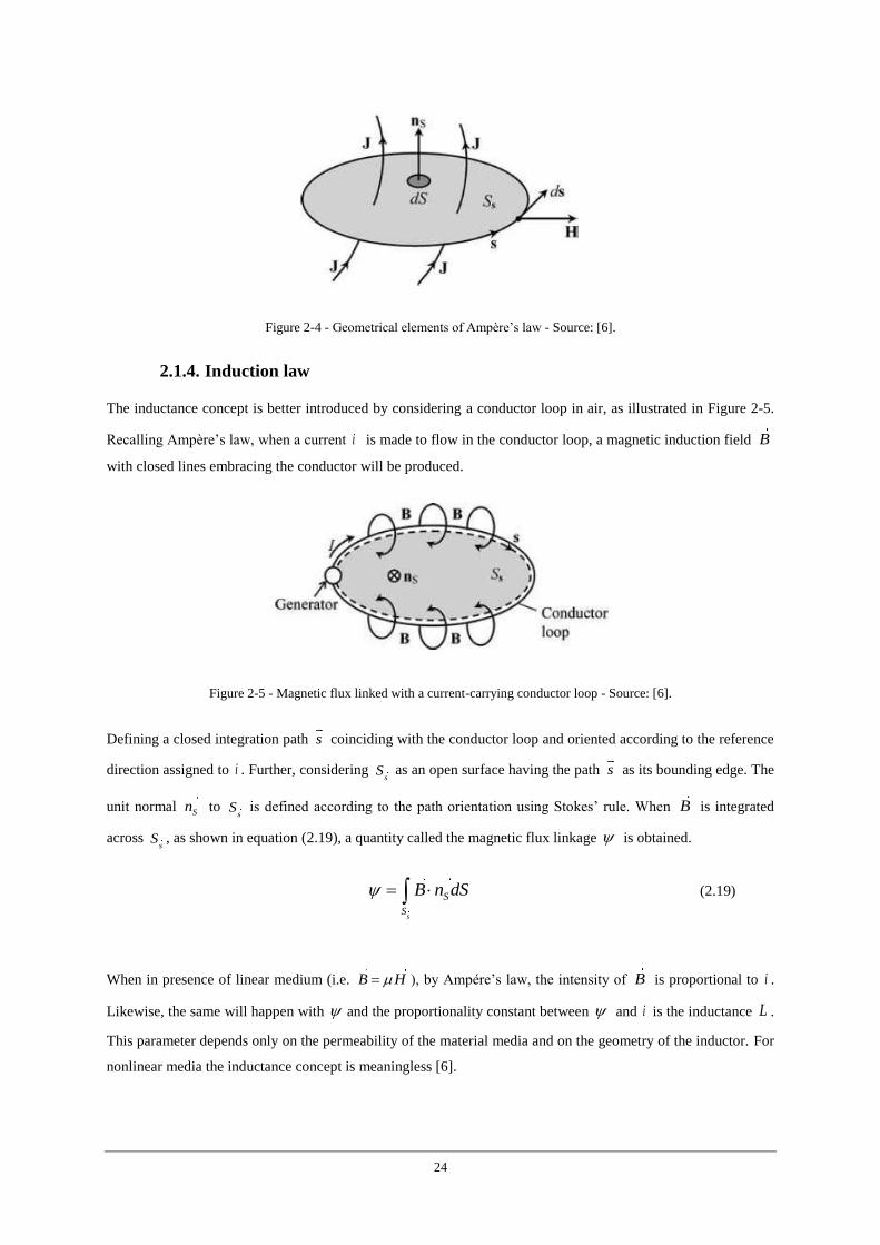
24

Figure 2-4 - Geometrical elements of Ampère’s law - Source: [6].

2.1.4. Induction law

The inductance concept is better introduced by considering a conductor loop in air, as illustrated in Figure 2-5.

Recalling Ampère’s law, when a current i is made to flow in the conductor loop, a magnetic induction field B

with closed lines embracing the conductor will be produced.

Figure 2-5 - Magnetic flux linked with a current-carrying conductor loop - Source: [6].

Defining a closed integration path s coinciding with the conductor loop and oriented according to the reference

direction assigned to i . Further, considering s

S as an open surface having the path s as its bounding edge. The

unit normal Sn to s

S is defined according to the path orientation using Stokes’ rule. When B is integrated

across s

S , as shown in equation (2.19), a quantity called the magnetic flux linkage is obtained.

s

S

S

B n dS (2.19)

When in presence of linear medium (i.e. B H ), by Ampére’s law, the intensity of B is proportional to i .

Likewise, the same will happen with and the proportionality constant between and i is the inductance L .

This parameter depends only on the permeability of the material media and on the geometry of the inductor. For

nonlinear media the inductance concept is meaningless [6].

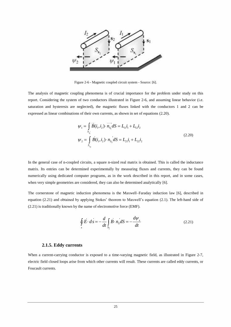
25

Figure 2-6 - Magnetic coupled circuit system - Source: [6].

The analysis of magnetic coupling phenomena is of crucial importance for the problem under study on this

report. Considering the system of two conductors illustrated in Figure 2-6, and assuming linear behavior (i.e.

saturation and hysteresis are neglected), the magnetic fluxes linked with the conductors 1 and 2 can be

expressed as linear combinations of their own currents, as shown in set of equations (2.20).

1

1

2

2

1 1 2 11 1 12 2

2 1 2 21 1 22 2

( , )

( , )

s

s

S

S

S

S

B i i n dS L i L i

B i i n dS L i L i

(2.20)

In the general case of n-coupled circuits, a square n-sized real matrix is obtained. This is called the inductance

matrix. Its entries can be determined experimentally by measuring fluxes and currents, they can be found

numerically using dedicated computer programs, as in the work described in this report, and in some cases,

when very simple geometries are considered, they can also be determined analytically [6].

The cornerstone of magnetic induction phenomena is the Maxwell–Faraday induction law [6], described in

equation (2.21) and obtained by applying Stokes’ theorem to Maxwell’s equation (2.1). The left-hand side of

(2.21) is traditionally known by the name of electromotive force (EMF).

s

sS

Ss

ddE d s B n dS

dt dt

(2.21)

2.1.5. Eddy currents

When a current-carrying conductor is exposed to a time-varying magnetic field, as illustrated in Figure 2-7,

electric field closed loops arise from which other currents will result. These currents are called eddy currents, or

Foucault currents.

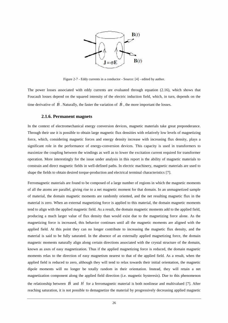
26

Figure 2-7 - Eddy currents in a conductor - Source: [4] - edited by author.

The power losses associated with eddy currents are evaluated through equation (2.16), which shows that

Foucault losses depend on the squared intensity of the electric induction field, which, in turn, depends on the

time derivative of B . Naturally, the faster the variation of B , the more important the losses.

2.1.6. Permanent magnets

In the context of electromechanical energy conversion devices, magnetic materials take great preponderance.

Through their use it is possible to obtain large magnetic flux densities with relatively low levels of magnetizing

force, which, considering magnetic forces and energy density increase with increasing flux density, plays a

significant role in the performance of energy-conversion devices. This capacity is used in transformers to

maximize the coupling between the windings as well as to lower the excitation current required for transformer

operation. More interestingly for the issue under analysis in this report is the ability of magnetic materials to

constrain and direct magnetic fields in well-defined paths. In electric machinery, magnetic materials are used to

shape the fields to obtain desired torque-production and electrical terminal characteristics [7].

Ferromagnetic materials are found to be composed of a large number of regions in which the magnetic moments

of all the atoms are parallel, giving rise to a net magnetic moment for that domain. In an unmagnetized sample

of material, the domain magnetic moments are randomly oriented, and the net resulting magnetic flux in the

material is zero. When an external magnetizing force is applied to this material, the domain magnetic moments

tend to align with the applied magnetic field. As a result, the domain magnetic moments add to the applied field,

producing a much larger value of flux density than would exist due to the magnetizing force alone. As the

magnetizing force is increased, this behavior continues until all the magnetic moments are aligned with the

applied field. At this point they can no longer contribute to increasing the magnetic flux density, and the

material is said to be fully saturated. In the absence of an externally applied magnetizing force, the domain

magnetic moments naturally align along certain directions associated with the crystal structure of the domain,

known as axes of easy magnetization. Thus if the applied magnetizing force is reduced, the domain magnetic

moments relax to the direction of easy magnetism nearest to that of the applied field. As a result, when the

applied field is reduced to zero, although they will tend to relax towards their initial orientation, the magnetic

dipole moments will no longer be totally random in their orientation. Instead, they will retain a net

magnetization component along the applied field direction (i.e. magnetic hysteresis). Due to this phenomenon

the relationship between B and H for a ferromagnetic material is both nonlinear and multivalued [7]. After

reaching saturation, it is not possible to demagnetize the material by progressively decreasing applied magnetic

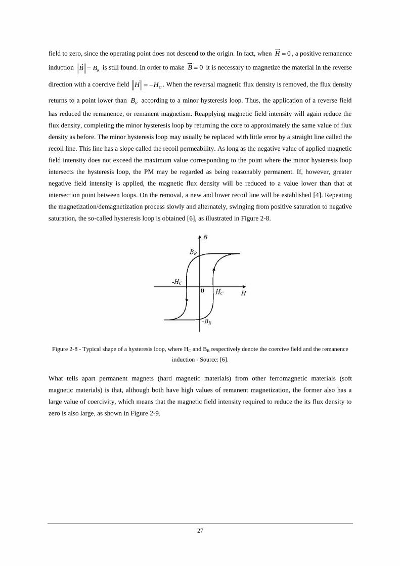
27

field to zero, since the operating point does not descend to the origin. In fact, when 0H , a positive remanence

induction RB B is still found. In order to make 0B it is necessary to magnetize the material in the reverse

direction with a coercive field CH H . When the reversal magnetic flux density is removed, the flux density

returns to a point lower than RB according to a minor hysteresis loop. Thus, the application of a reverse field

has reduced the remanence, or remanent magnetism. Reapplying magnetic field intensity will again reduce the

flux density, completing the minor hysteresis loop by returning the core to approximately the same value of flux

density as before. The minor hysteresis loop may usually be replaced with little error by a straight line called the

recoil line. This line has a slope called the recoil permeability. As long as the negative value of applied magnetic

field intensity does not exceed the maximum value corresponding to the point where the minor hysteresis loop

intersects the hysteresis loop, the PM may be regarded as being reasonably permanent. If, however, greater

negative field intensity is applied, the magnetic flux density will be reduced to a value lower than that at

intersection point between loops. On the removal, a new and lower recoil line will be established [4]. Repeating

the magnetization/demagnetization process slowly and alternately, swinging from positive saturation to negative

saturation, the so-called hysteresis loop is obtained [6], as illustrated in Figure 2-8.

Figure 2-8 - Typical shape of a hysteresis loop, where HC and BR respectively denote the coercive field and the remanence

induction - Source: [6].

What tells apart permanent magnets (hard magnetic materials) from other ferromagnetic materials (soft

magnetic materials) is that, although both have high values of remanent magnetization, the former also has a

large value of coercivity, which means that the magnetic field intensity required to reduce the its flux density to

zero is also large, as shown in Figure 2-9.

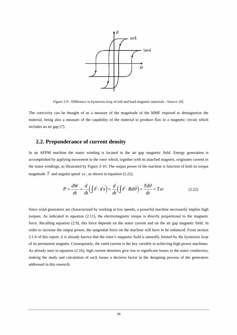
28

Figure 2-9 - Difference in hysteresis loop of soft and hard magnetic materials - Source: [6].

The coercivity can be thought of as a measure of the magnitude of the MMF required to demagnetize the

material, being also a measure of the capability of the material to produce flux in a magnetic circuit which

includes an air gap [7].

2.2. Preponderance of current density

In an AFPM machine the stator winding is located in the air gap magnetic field. Energy generation is

accomplished by applying movement to the rotor which, together with its attached magnets, originates current in

the stator windings, as illustrated by Figure 2-10. The output power of the machine is function of both its torque

magnitude T and angular speed , as shown in equation (2.22).

dW d d TdP F d x F Rd T

dt dt dt dt

(2.22)

Since wind generators are characterized by working at low speeds, a powerful machine necessarily implies high

torques. As indicated in equation (2.11), the electromagnetic torque is directly proportional to the magnetic

force. Recalling equation (2.9), this force depends on the stator current and on the air gap magnetic field. In

order to increase the output power, the tangential force on the machine will have to be enhanced. From section

2.1.6 of this report, it is already known that the rotor’s magnetic field is naturally limited by the hysteresis loop

of its permanent magnets. Consequently, the rated current is the key variable in achieving high power machines.

As already seen in equation (2.16), high current densities give rise to significant losses in the stator conductors,

making the study and calculation of such losses a decisive factor in the designing process of the generators

addressed in this research.

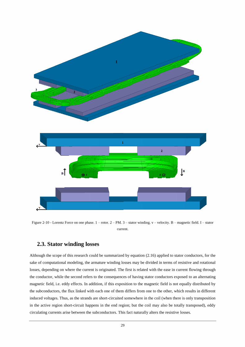
29

Figure 2-10 - Lorentz Force on one phase. 1 – rotor. 2 – PM. 3 – stator winding. v – velocity. B – magnetic field. I – stator

current.

2.3. Stator winding losses

Although the scope of this research could be summarized by equation (2.16) applied to stator conductors, for the

sake of computational modeling, the armature winding losses may be divided in terms of resistive and rotational

losses, depending on where the current is originated. The first is related with the ease in current flowing through

the conductor, while the second refers to the consequences of having stator conductors exposed to an alternating

magnetic field, i.e. eddy effects. In addition, if this exposition to the magnetic field is not equally distributed by

the subconductors, the flux linked with each one of them differs from one to the other, which results in different

induced voltages. Thus, as the strands are short-circuited somewhere in the coil (when there is only transposition

in the active region short-circuit happens in the end region; but the coil may also be totally transposed), eddy

circulating currents arise between the subconductors. This fact naturally alters the resistive losses.

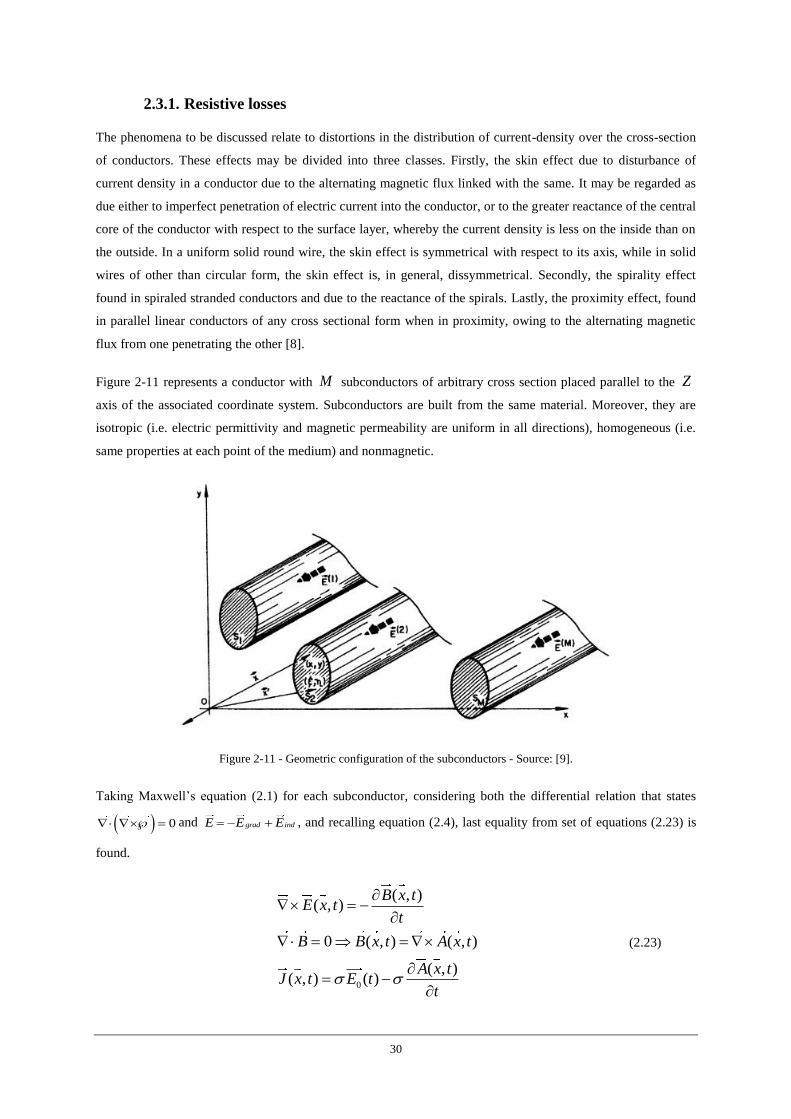
30

2.3.1. Resistive losses

The phenomena to be discussed relate to distortions in the distribution of current-density over the cross-section

of conductors. These effects may be divided into three classes. Firstly, the skin effect due to disturbance of

current density in a conductor due to the alternating magnetic flux linked with the same. It may be regarded as

due either to imperfect penetration of electric current into the conductor, or to the greater reactance of the central

core of the conductor with respect to the surface layer, whereby the current density is less on the inside than on

the outside. In a uniform solid round wire, the skin effect is symmetrical with respect to its axis, while in solid

wires of other than circular form, the skin effect is, in general, dissymmetrical. Secondly, the spirality effect

found in spiraled stranded conductors and due to the reactance of the spirals. Lastly, the proximity effect, found

in parallel linear conductors of any cross sectional form when in proximity, owing to the alternating magnetic

flux from one penetrating the other [8].

Figure 2-11 represents a conductor with M subconductors of arbitrary cross section placed parallel to the Z

axis of the associated coordinate system. Subconductors are built from the same material. Moreover, they are

isotropic (i.e. electric permittivity and magnetic permeability are uniform in all directions), homogeneous (i.e.

same properties at each point of the medium) and nonmagnetic.

Figure 2-11 - Geometric configuration of the subconductors - Source: [9].

Taking Maxwell’s equation (2.1) for each subconductor, considering both the differential relation that states

0 and grad indE E E , and recalling equation (2.4), last equality from set of equations (2.23) is

found.

0

( , )( , )

0 ( , ) ( , )

( , )( , ) ( )

B x tE x t

t

B B x t A x t

A x tJ x t E t

t

(2.23)

31

t is the time array, x is a generic vector in the XY plan, J is the current density, is the electrical

conductivity, 0E is the electric field applied to the subconductor (e.g. gradE ), and A is the magnetic vector

potential.

Disregarding the displacement current and endpoint effects (i.e. end winding region), and assuming an uniform

, then 0E , A and J have only the longitudinal component (i.e. along Z direction) [9].

Since both fields and currents are periodic and, therefore, harmonic functions of time, it is possible to separate

spatial and temporal dependencies in equation (2.23), considering that the system is in the steady state [9].

Therefore, phasor notation can be used and last equality from set of equations (2.24) is obtained.

0

ind M

ind

J j A

J E J

(2.24)

It is also possible to express the magnetic vector potential in terms of the current density vector by means of

Maxwell’s equation (2.3), as shown in set of equations (2.25).

2

H J B J

A J

A A A A J

(2.25)

Assuming the Coulomb gauge condition 0A , 2

A J is reached, which results in the component

form expressed in set of equations (2.26).

2

2

2

x x

y y

z z

A J

A J

A J

(2.26)

In fact, set of equations (2.26) is nothing less than Poisson's equation three times over, thus it is possible to

immediately write its unique solutions, which are presented in set of equations (2.27).

32

4

4

4

y

y

y

xx

x

zz

z

JA dy

r

JA dx

r

JA dz

r

(2.27)

These solutions can be recombined to form the single vector solution of equation (2.28).

4 V

JA dV

r

(2.28)

Recalling equation (2.24), the magnetic vector potential in ( , )x y because of a filamentary current in 0( , , )z

can be written in scalar form as shown in equation (2.29) [9].

0 01

2 2 2 2

0

( , )( , , )

4

j JJ x y z E d d dz

x y z z

(2.29)

The longitudinal component dependency can be surpassed by solving the integral along the length of the

conductor. The volume integral turns into a surface integral as shown in equation (2.30).

1

2 2 2

0( , ) ( , ) lnS

J x y E J x y d d (2.30)

J and 0E are complex quantities in the Z axis direction, while the constant is the eigenvalue of the

integral equation defined by (2.31).

jf (2.31)

j is the imaginary unit, f is the frequency of the field and is the magnetic permeability of the

subconductor.

Generalizing equation (2.30) to the whole conductor with its M subconductors, integral equation (2.32) is

found for the generic subconductor p .

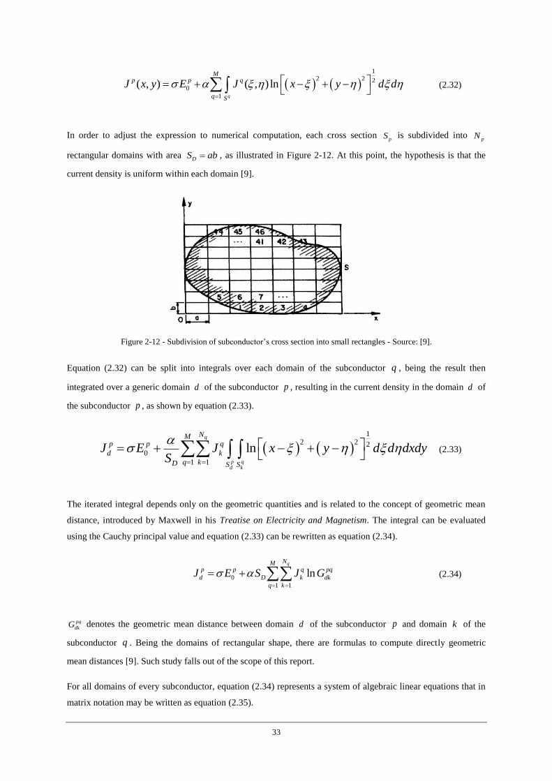
33

1

2 2 2

0

1

( , ) ( , ) lnq

Mp p q

q S

J x y E J x y d d

(2.32)

In order to adjust the expression to numerical computation, each cross section pS is subdivided into

pN

rectangular domains with area DS ab , as illustrated in Figure 2-12. At this point, the hypothesis is that the

current density is uniform within each domain [9].

Figure 2-12 - Subdivision of subconductor’s cross section into small rectangles - Source: [9].

Equation (2.32) can be split into integrals over each domain of the subconductor q , being the result then

integrated over a generic domain d of the subconductor p , resulting in the current density in the domain d of

the subconductor p , as shown by equation (2.33).

1

2 2 2

0

1 1

lnq

p qd k

NMp p q

d k

q kD S S

J E J x y d d dxdyS

(2.33)

The iterated integral depends only on the geometric quantities and is related to the concept of geometric mean

distance, introduced by Maxwell in his Treatise on Electricity and Magnetism. The integral can be evaluated

using the Cauchy principal value and equation (2.33) can be rewritten as equation (2.34).

0

1 1

lnqNM

p p q pq

d D k dk

q k

J E S J G

(2.34)

pq

dkG denotes the geometric mean distance between domain d of the subconductor p and domain k of the

subconductor q . Being the domains of rectangular shape, there are formulas to compute directly geometric

mean distances [9]. Such study falls out of the scope of this report.

For all domains of every subconductor, equation (2.34) represents a system of algebraic linear equations that in

matrix notation may be written as equation (2.35).

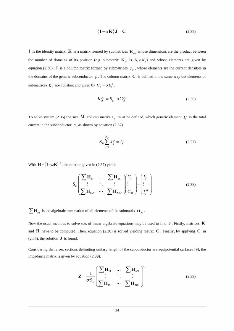
34

I K J C (2.35)

I is the identity matrix. K is a matrix formed by submatrices pqK whose dimensions are the product between

the number of domains of its position (e.g. submatrix 21K is

1 2N N ) and whose elements are given by

equation (2.36). J is a column matrix formed by submatrices pJ , whose elements are the current densities in

the domains of the generic subconductor p . The column matrix C is defined in the same way but elements of

submatrices pC are constant and given by 0

p

pC E .

lnpq pq

dk D dkK S G (2.36)

To solve system (2.35) the size M column matrix TI must be defined, which generic element p

TI is the total

current in the subconductor p , as shown by equation (2.37).

1

pN

p p

D j T

j

S J I

(2.37)

With 1

H I K , the relation given in (2.37) yields

1

111 1

1

TM

D

MM MM M T

C I

S

C I

H H

H H

(2.38)

pqH is the algebraic summation of all elements of the submatrix pqH .

Now the usual methods to solve sets of linear algebraic equations may be used to find J . Firstly, matrices K

and H have to be computed. Then, equation (2.38) is solved yielding matrix C . Finally, by applying C in

(2.35), the solution J is found.

Considering that cross sections delimiting unitary length of the subconductor are equipotential surfaces [9], the

impedance matrix is given by equation (2.39).

1

11 1

1

1M

D

M MM

S

H H

Z

H H

(2.39)

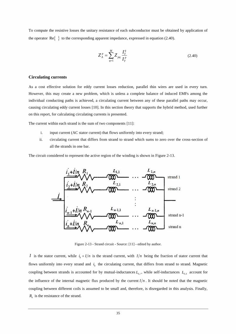
35

To compute the resistive losses the unitary resistance of each subconductor must be obtained by application of

the operator Re to the corresponding apparent impedance, expressed in equation (2.40).

1

qMp TA pq p

q T

IZ Z

I

(2.40)

Circulating currents

As a cost effective solution for eddy current losses reduction, parallel thin wires are used in every turn.

However, this may create a new problem, which is unless a complete balance of induced EMFs among the

individual conducting paths is achieved, a circulating current between any of these parallel paths may occur,

causing circulating eddy current losses [10]. In this section theory that supports the hybrid method, used further

on this report, for calculating circulating currents is presented.

The current within each strand is the sum of two components [11]:

i. input current (AC stator current) that flows uniformly into every strand;

ii. circulating current that differs from strand to strand which sums to zero over the cross-section of

all the strands in one bar.

The circuit considered to represent the active region of the winding is shown in Figure 2-13.

Figure 2-13 - Strand circuit - Source: [11] - edited by author.

I is the stator current, while ki I n is the strand current, with I n being the fraction of stator current that

flows uniformly into every strand and ki the circulating current, that differs from strand to strand. Magnetic

coupling between strands is accounted for by mutual-inductances,k lL , while self-inductances

,k kL account for

the influence of the internal magnetic flux produced by the current I n . It should be noted that the magnetic

coupling between different coils is assumed to be small and, therefore, is disregarded in this analysis. Finally,

kR is the resistance of the strand.

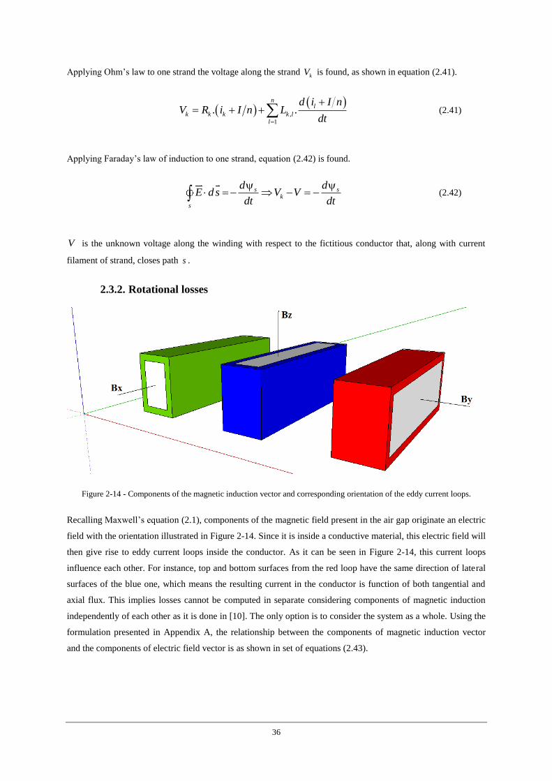
36

Applying Ohm’s law to one strand the voltage along the strand kV is found, as shown in equation (2.41).

,

1

. .n

l

k k k k l

l

d i I nV R i I n L

dt

(2.41)

Applying Faraday’s law of induction to one strand, equation (2.42) is found.

s sk

s

d dE ds V V

dt dt

(2.42)

V is the unknown voltage along the winding with respect to the fictitious conductor that, along with current

filament of strand, closes path s .

2.3.2. Rotational losses

Figure 2-14 - Components of the magnetic induction vector and corresponding orientation of the eddy current loops.

Recalling Maxwell’s equation (2.1), components of the magnetic field present in the air gap originate an electric

field with the orientation illustrated in Figure 2-14. Since it is inside a conductive material, this electric field will

then give rise to eddy current loops inside the conductor. As it can be seen in Figure 2-14, this current loops

influence each other. For instance, top and bottom surfaces from the red loop have the same direction of lateral

surfaces of the blue one, which means the resulting current in the conductor is function of both tangential and

axial flux. This implies losses cannot be computed in separate considering components of magnetic induction

independently of each other as it is done in [10]. The only option is to consider the system as a whole. Using the

formulation presented in Appendix A, the relationship between the components of magnetic induction vector

and the components of electric field vector is as shown in set of equations (2.43).

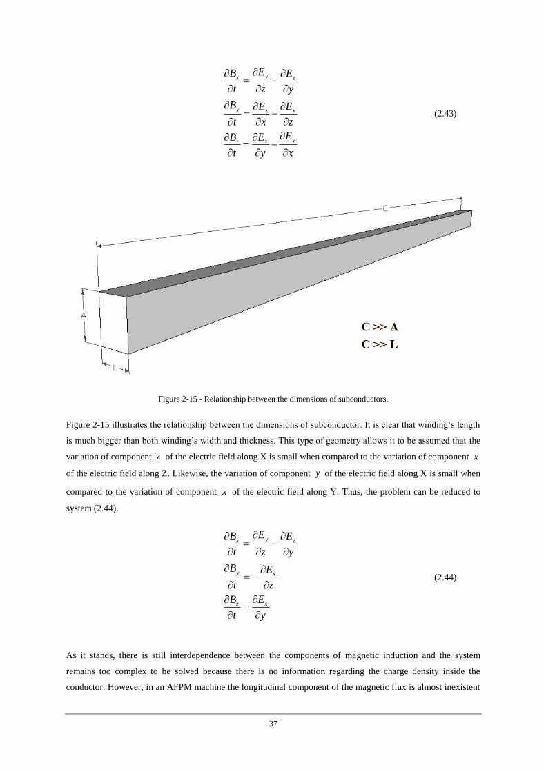
37

yx z

y xz

yxz

EB E

t z y

B EE

t x z

EEB

t y x

(2.43)

Figure 2-15 - Relationship between the dimensions of subconductors.

Figure 2-15 illustrates the relationship between the dimensions of subconductor. It is clear that winding’s length

is much bigger than both winding’s width and thickness. This type of geometry allows it to be assumed that the

variation of component z of the electric field along X is small when compared to the variation of component x

of the electric field along Z. Likewise, the variation of component y of the electric field along X is small when

compared to the variation of component x of the electric field along Y. Thus, the problem can be reduced to

system (2.44).

yx z

y x

xz

EB E

t z y

B E

t z

EB

t y

(2.44)

As it stands, there is still interdependence between the components of magnetic induction and the system

remains too complex to be solved because there is no information regarding the charge density inside the

conductor. However, in an AFPM machine the longitudinal component of the magnetic flux is almost inexistent

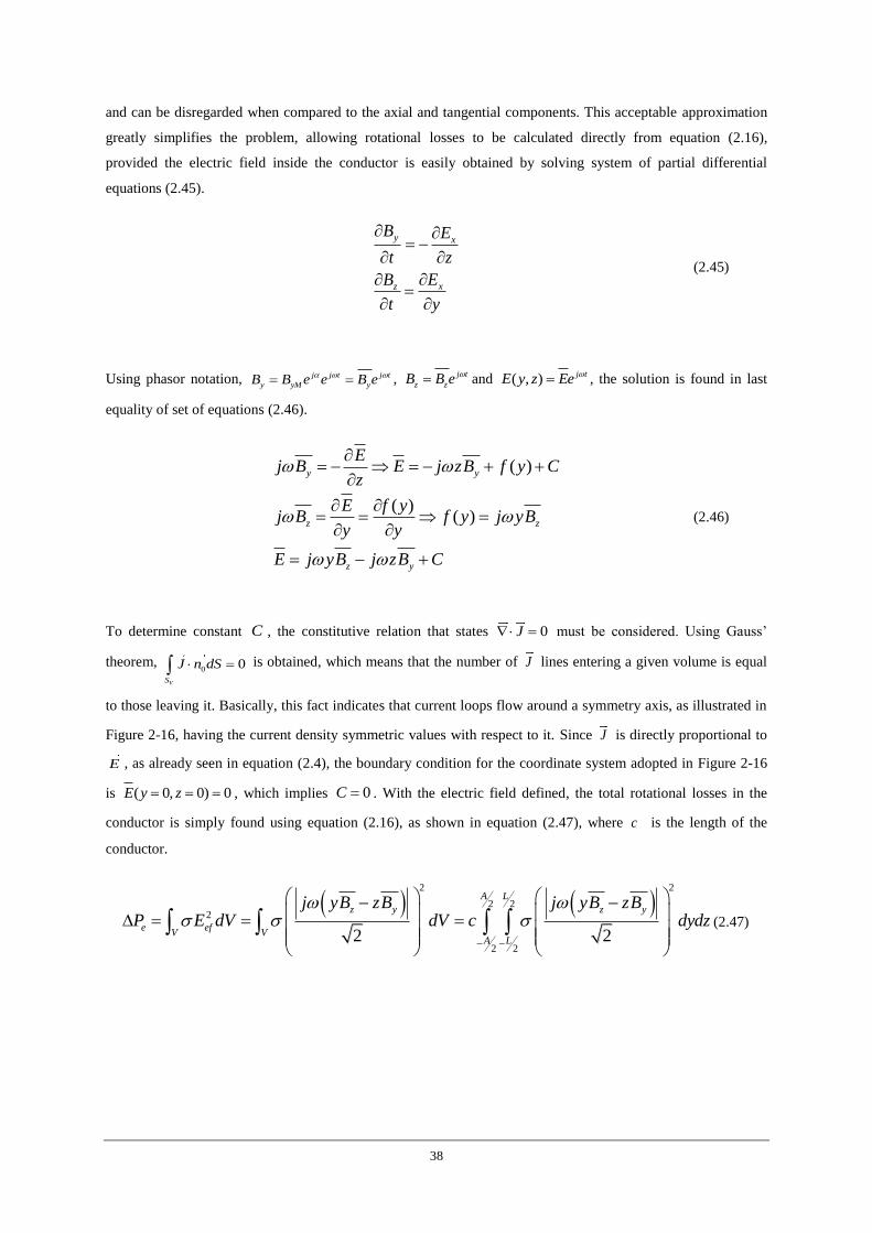
38

and can be disregarded when compared to the axial and tangential components. This acceptable approximation

greatly simplifies the problem, allowing rotational losses to be calculated directly from equation (2.16),

provided the electric field inside the conductor is easily obtained by solving system of partial differential

equations (2.45).

y x

xz

B E

t z

EB

t y

(2.45)

Using phasor notation, j j t j t

y yM yB B e e B e , j t

z zB B e and ( , ) j tE y z Ee , the solution is found in last

equality of set of equations (2.46).

( )

( )( )

y y

z z

z y

Ej B E j zB f y C

z

E f yj B f y j yB

y y

E j yB j zB C

(2.46)

To determine constant C , the constitutive relation that states 0J must be considered. Using Gauss’

theorem, 0 0

VS

J n dS is obtained, which means that the number of J lines entering a given volume is equal

to those leaving it. Basically, this fact indicates that current loops flow around a symmetry axis, as illustrated in

Figure 2-16, having the current density symmetric values with respect to it. Since J is directly proportional to

E , as already seen in equation (2.4), the boundary condition for the coordinate system adopted in Figure 2-16

is ( 0, 0) 0E y z , which implies 0C . With the electric field defined, the total rotational losses in the

conductor is simply found using equation (2.16), as shown in equation (2.47), where c is the length of the

conductor.

2 2

2 22

2 22 2

A L

z y z y

e efV V

A L

j yB zB j yB zBP E dV dV c dydz

(2.47)

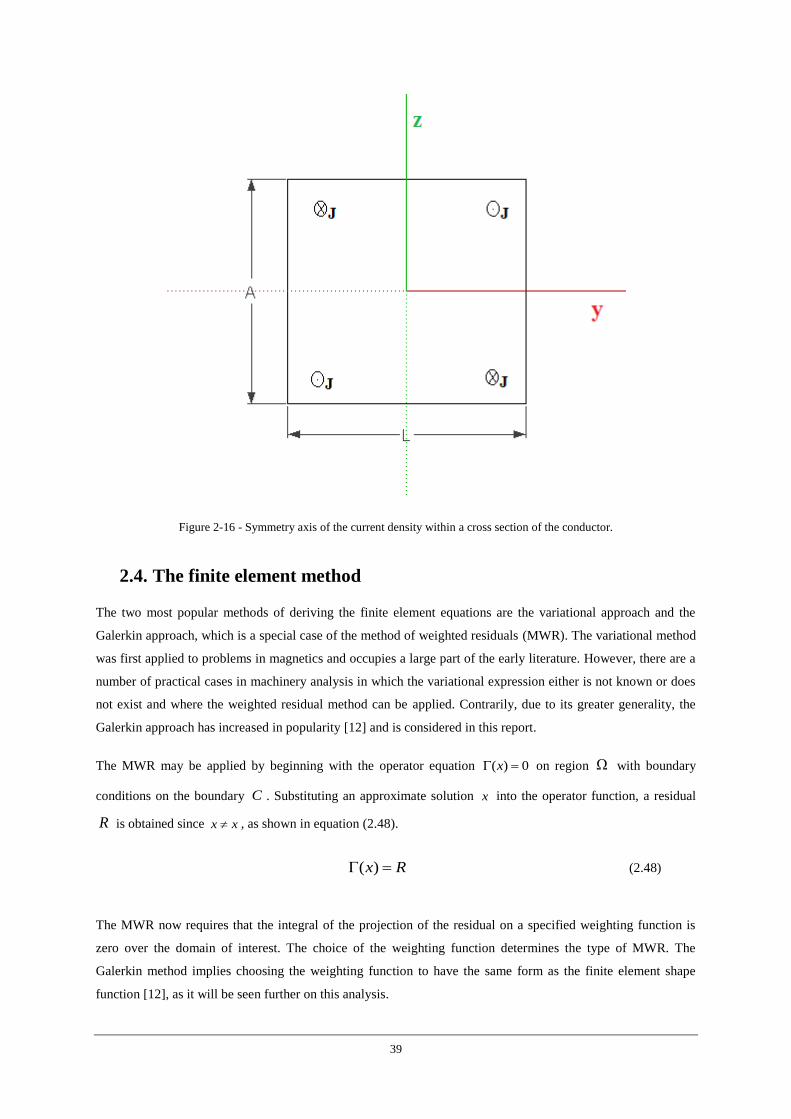
39

Figure 2-16 - Symmetry axis of the current density within a cross section of the conductor.

2.4. The finite element method

The two most popular methods of deriving the finite element equations are the variational approach and the

Galerkin approach, which is a special case of the method of weighted residuals (MWR). The variational method

was first applied to problems in magnetics and occupies a large part of the early literature. However, there are a

number of practical cases in machinery analysis in which the variational expression either is not known or does

not exist and where the weighted residual method can be applied. Contrarily, due to its greater generality, the

Galerkin approach has increased in popularity [12] and is considered in this report.

The MWR may be applied by beginning with the operator equation ( ) 0x on region with boundary

conditions on the boundary C . Substituting an approximate solution x into the operator function, a residual

R is obtained since x x , as shown in equation (2.48).

( )x R (2.48)

The MWR now requires that the integral of the projection of the residual on a specified weighting function is

zero over the domain of interest. The choice of the weighting function determines the type of MWR. The

Galerkin method implies choosing the weighting function to have the same form as the finite element shape

function [12], as it will be seen further on this analysis.

40

The time harmonic form of the diffusion equation with A as the unknown will be used as example. Such

equation was deducted in last equality of set of equations (2.25). For a linear two dimensional Cartesian

problem, the Laplacian on the left-hand side of the diffusion equation develops as shown in equation (2.49).

2 22

02 2

1 1 1A AA J j A

x y

(2.49)

As shown in equation (2.50), substituting A for an approximation A , a residual R is obtained.

2 2

02 2

1 1A AR J j A

x y

(2.50)

Now, as done in equation (2.51), the residual must be pondered with a weighting function W and the integral

over the region set to zero.

2 2

02 2

0

1 1

RWdxdy

A AW dxdy j W Adxdy W J dxdy

x y

(2.51)

Recalling that integration by parts states that ( ) '( ) ( ) ( ) '( ) ( )u x v x dx u x v x u x v x dx , by making

2 2

2 2

1 1'

A Av

x y

and u W , first term of last equality of equation (2.51) can be integrated as shown in

equation (2.52), where the last term is on the boundary C with n being the outward normal unit vector.

2 2

2 2

1 1

1 1

C

A AW dxdy

x y

W A W A Adxdy W dc

x x y y n

(2.52)

Substituting equation (2.52) into equation (2.51), it is possible to break the surface into summations over small

areas, as shown in equation (2.53). For instance, the surface may be meshed with M triangles (the finite

elements) and replace the integral over the entire domain with the summation of the integral over the individual

triangles.

41

1

0

1

1

e

e

e

e e e e

eM

e

e e e e

e C

e e

W A W Adxdy

x x y y

Aj W A dxdy W dc

n

J W dxdy

(2.53)

The line integral in equation (2.53) only needs to be evaluated over elements which have a side in common with

the boundary of the problem. Usually, this integral is simply set to zero implying that 0A

n

which results in

the so called natural boundary condition. However, this integral is often used in problems in which the finite

element method is coupled with other solution techniques (e.g. air gap elements calculations). In this case the

integral must be evaluated. Considering a triangular element with vertices i , j , k , at coordinates ( , )i ix y ,

( , )j jx y , ( , )k kx y , respectively. The vertices are nodes at which the unknown vector potentials will eventually

be calculated. Assuming the potential varies linearly in the element, a linear or first order element is obtained.

With this approximation, it is possible to express the vector potential at any point in the triangle as shown in

equation (2.54).

1 2 3A C C x C y (2.54)

1C , 2C and

3C are constants to be determined. Is shall be noted that since the vector potential varies linearly,

the flux density, which is the derivative of the potential, is constant in the triangle. At point ( , )i ix y , A must be

equal to iA , with the same happening for nodes j and k . Thus, system of equations (2.55) is obtained, which

shall be solved for 1C ,

2C and 3C in terms of the potential and geometry using Cramer’s rule. The results are

expressed in set of equations (2.56).

1 2 3

1 2 3

1 2 3

i i i

j j j

k k k

A C C x C y

A C C x C y

A C C x C y

(2.55)

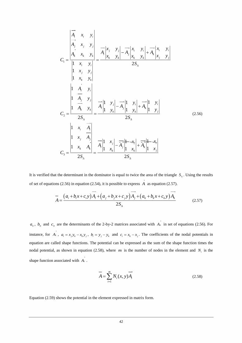
42

1

2

3

1 2

1

1

1

111 1

1 11 1

2 2

1

11

1 1

2

i i i

j j j

i ij j i i

i j kk k k

j jk k k k

i i

j j

k k

i i

j j

ij i

i j kk k

jk k

i i

j j

j

ik k

A x y

A x yx yx y x y

A A AA x y x yx y x yC

x y S

x y

x y

A y

A yyy y

A A AA y yy yC

S S

x A

x Ax

Ax A xC

S

11

11

2

ii

j k

jk k

xxA A

xx

S

(2.56)

It is verified that the determinant in the dominator is equal to twice the area of the triangle S. Using the results

of set of equations (2.56) in equation (2.54), it is possible to express A as equation (2.57).

2

i i i i j j j j k k k ka b x c y A a b x c y A a b x c y AA

S

(2.57)

na , nb and nc are the determinants of the 2-by-2 matrices associated with nA in set of equations (2.56). For

instance, for iA , i j k k ja x y x y ,

i j kb y y and i k jc x x . The coefficients of the nodal potentials in

equation are called shape functions. The potential can be expressed as the sum of the shape function times the

nodal potential, as shown in equation (2.58), where m is the number of nodes in the element and iN is the

shape function associated with iA .

1

( , )m

i i

i

A N x y A

(2.58)

Equation (2.59) shows the potential in the element expressed in matrix form.

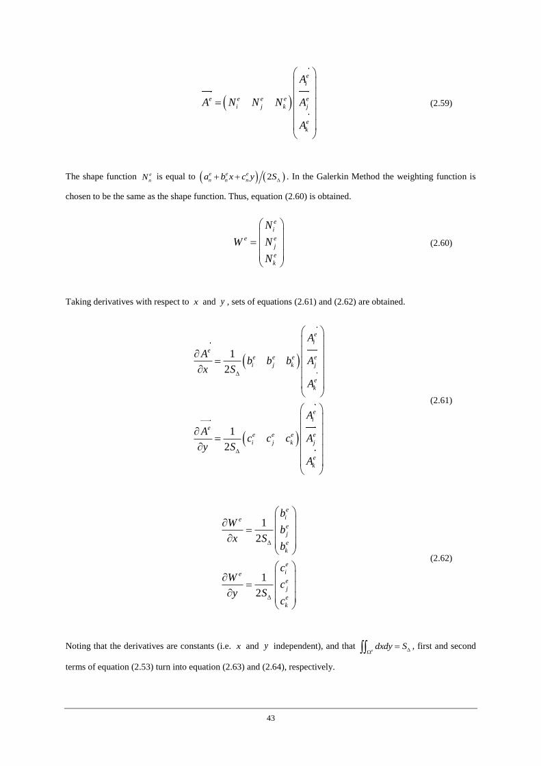
43

e

i

e e e e e

i j k j

e

k

A

A N N N A

A

(2.59)

The shape function e

nN is equal to 2e e e

n n na b x c y S . In the Galerkin Method the weighting function is

chosen to be the same as the shape function. Thus, equation (2.60) is obtained.

e

i

e e

j

e

k

N

W N

N

(2.60)

Taking derivatives with respect to x and y , sets of equations (2.61) and (2.62) are obtained.

1

2

1

2

e

i

ee e e e

i j k j

e

k

e

i

ee e e e

i j k j

e

k

A

Ab b b A

x S

A

A

Ac c c A

y S

A

(2.61)

1

2

1

2

e

iee

j

e

k

e

iee

j

e

k

bW

bx S

b

cW

cy S

c

(2.62)

Noting that the derivatives are constants (i.e. x and y independent), and that edxdy S

, first and second

terms of equation (2.53) turn into equation (2.63) and (2.64), respectively.

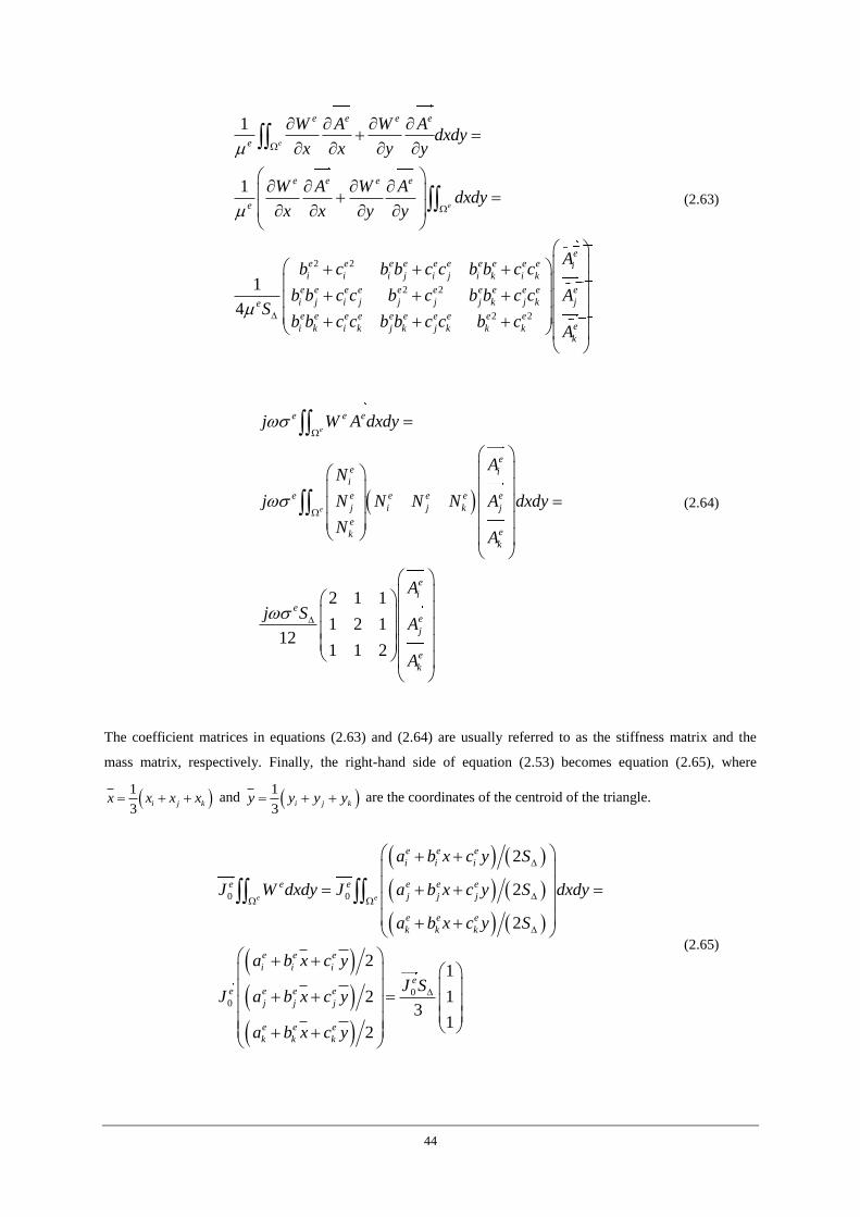
44

2 2

2 2

2 2

1

1

1

4

e

e

e e e e

e

e e e e

e

e e e e e e e e e e

i i i j i j i k i k

e e e e e e e e e e

i j i j j j j k j ke

e e e e e e e e e e

i k i k j k j k k k

W A W Adxdy

x x y y

W A W Adxdy

x x y y

b c b b c c b b c c

b b c c b c b b c cS

b b c c b b c c b c

e

i

e

j

e

k

A

A

A

(2.63)

2 1 1

1 2 112

1 1 2

e

e

e e e

ee ii

e e e e e e

j i j k j

eekk

e

i

ee

j

e

k

j W A dxdy

AN

j N N N N A dxdy

NA

A

j SA

A

(2.64)

The coefficient matrices in equations (2.63) and (2.64) are usually referred to as the stiffness matrix and the

mass matrix, respectively. Finally, the right-hand side of equation (2.53) becomes equation (2.65), where

1

3i j kx x x x and

1

3i j ky y y y are the coordinates of the centroid of the triangle.

0 0

00

2

2

2

21

2 13

12

e e

e e e

i i i

e e e e e e

j j j

e e e

k k k

e e e

i i i

ee e e e

j j j

e e e

k k k

a b x c y S

J W dxdy J a b x c y S dxdy

a b x c y S

a b x c y

J SJ a b x c y

a b x c y

(2.65)

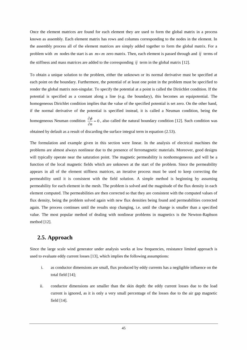
45

Once the element matrices are found for each element they are used to form the global matrix in a process

known as assembly. Each element matrix has rows and columns corresponding to the nodes in the element. In

the assembly process all of the element matrices are simply added together to form the global matrix. For a

problem with m nodes the start is an m m zero matrix. Then, each element is passed through and ij terms of

the stiffness and mass matrices are added to the corresponding ij term in the global matrix [12].

To obtain a unique solution to the problem, either the unknown or its normal derivative must be specified at

each point on the boundary. Furthermore, the potential of at least one point in the problem must be specified to

render the global matrix non-singular. To specify the potential at a point is called the Diriichlet condition. If the

potential is specified as a constant along a line (e.g. the boundary), this becomes an equipotential. The

homogeneous Dirichlet condition implies that the value of the specified potential is set zero. On the other hand,

if the normal derivative of the potential is specified instead, it is called a Neuman condition, being the

homogeneous Neuman condition 0n

, also called the natural boundary condition [12]. Such condition was

obtained by default as a result of discarding the surface integral term in equation (2.53).

The formulation and example given in this section were linear. In the analysis of electrical machines the

problems are almost always nonlinear due to the presence of ferromagnetic materials. Moreover, good designs

will typically operate near the saturation point. The magnetic permeability is nonhomogeneous and will be a

function of the local magnetic fields which are unknown at the start of the problem. Since the permeability

appears in all of the element stiffness matrices, an iterative process must be used to keep correcting the

permeability until it is consistent with the field solution. A simple method is beginning by assuming

permeability for each element in the mesh. The problem is solved and the magnitude of the flux density in each

element computed. The permeabilities are then corrected so that they are consistent with the computed values of

flux density, being the problem solved again with new flux densities being found and permeabilities corrected

again. The process continues until the results stop changing, i.e. until the change is smaller than a specified

value. The most popular method of dealing with nonlinear problems in magnetics is the Newton-Raphson

method [12].

2.5. Approach

Since the large scale wind generator under analysis works at low frequencies, resistance limited approach is

used to evaluate eddy current losses [13], which implies the following assumptions:

i. as conductor dimensions are small, flux produced by eddy currents has a negligible influence on the

total field [14];

ii. conductor dimensions are smaller than the skin depth: the eddy current losses due to the load

current is ignored, as it is only a very small percentage of the losses due to the air gap magnetic

field [14].

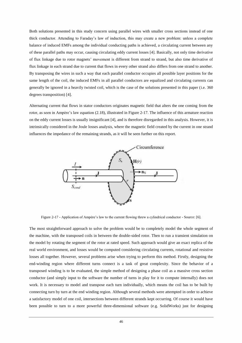
46

Both solutions presented in this study concern using parallel wires with smaller cross sections instead of one

thick conductor. Attending to Faraday’s law of induction, this may create a new problem: unless a complete

balance of induced EMFs among the individual conducting paths is achieved, a circulating current between any

of these parallel paths may occur, causing circulating eddy current losses [4]. Basically, not only time derivative

of flux linkage due to rotor magnets’ movement is different from strand to strand, but also time derivative of

flux linkage in each strand due to current that flows in every other strand also differs from one strand to another.

By transposing the wires in such a way that each parallel conductor occupies all possible layer positions for the

same length of the coil, the induced EMFs in all parallel conductors are equalized and circulating currents can

generally be ignored in a heavily twisted coil, which is the case of the solutions presented in this paper (i.e. 360

degrees transposition) [4].

Alternating current that flows in stator conductors originates magnetic field that alters the one coming from the

rotor, as seen in Ampère’s law equation (2.18), illustrated in Figure 2-17. The influence of this armature reaction

on the eddy current losses is usually insignificant [4], and is therefore disregarded in this analysis. However, it is

intrinsically considered in the Joule losses analysis, where the magnetic field created by the current in one strand

influences the impedance of the remaining strands, as it will be seen further on this report.

Figure 2-17 - Application of Ampère’s law to the current flowing threw a cylindrical conductor - Source: [6].

The most straightforward approach to solve the problem would be to completely model the whole segment of

the machine, with the transposed coils in between the double-sided rotor. Then to run a transient simulation on

the model by rotating the segment of the rotor at rated speed. Such approach would give an exact replica of the

real world environment, and losses would be computed considering circulating currents, rotational and resistive

losses all together. However, several problems arise when trying to perform this method. Firstly, designing the

end-winding region where different turns connect is a task of great complexity. Since the behavior of a

transposed winding is to be evaluated, the simple method of designing a phase coil as a massive cross section

conductor (and simply input to the software the number of turns in play for it to compute internally) does not

work. It is necessary to model and transpose each turn individually, which means the coil has to be built by

connecting turn by turn at the end winding region. Although several methods were attempted in order to achieve

a satisfactory model of one coil, intersections between different strands kept occurring. Of course it would have

been possible to turn to a more powerful three-dimensional software (e.g. SolidWorks) just for designing

47

purposes and then convert it into a Maxwell model, but two reasons advised to search for other solutions: 1. the

idea of testing cases with several situations (i.e. several number of strands and different types of winding)

required the coding to be kept only about the Maxwell environment; 2. analysis were performed on the active

region devoid of the end-winding region, and a considerably amount of time was consumed just to compute the

initial mesh, so, even considering a good design of the coil, with the end region, was achieved, simulation would

most likely not return any results due to lack of computational power. Moreover, the method followed to

calculate eddy current losses allows a solution to be found in a magnetostatic environment, since field

periodically variation can be computed using Fourier analysis along pole-pitch. To run a transient solution type

would not only be an uncertain step considering the complexity of the design itself, but would also produce

losses results that would not allow distinctions to be made between resistive and rotational losses. Consequently,

it would not be possible to depict losses sources of each solution and understand what can be changed to achieve

a more competitive winding.

Considering the above, rotational and resistive losses are studied separately with the influence of circulating

currents also being considered in a dedicated script and only then included as part of resistive losses.

48

49

Chapter 3

3. Simulation

The goal of this chapter is to describe in detail the computational methods used to calculate stator winding

losses. Firstly, the three-dimensional model of the segment used to study the machine is presented, with special

emphasis being given to the architecture of the two transposed winding technologies under analysis. Results for

resistive and rotational losses are presented and the critical aspects behind the methods’ algorithms discussed.

50

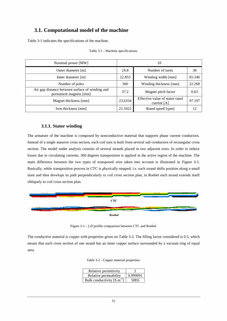
51

3.1. Computational model of the machine

Table 3-1 indicates the specifications of the machine.

Table 3-1 - Machine specifications.

Nominal power [MW] 10

Outer diameter [m] 24.8 Number of turns 38

Inner diameter [m] 22.853 Winding width [mm] 65.346

Number of poles 360 Winding thickness [mm] 22.268

Air gap distance between surface of winding and

permanent magnets [mm] 37.2 Magnet pitch factor 0.63

Magnet thickness [mm] 23.6334 Effective value of stator rated

current [A] 97.197

Iron thickness [mm] 21.1022 Rated speed [rpm] 12

3.1.1. Stator winding

The armature of the machine is composed by nonconductive material that supports phase current conductors.

Instead of a single massive cross section, each coil turn is built from several sub conductors of rectangular cross

section. The model under analysis consists of several strands placed in two adjacent rows. In order to reduce

losses due to circulating currents, 360 degrees transposition is applied in the active region of the machine. The

main difference between the two types of transposed wire taken into account is illustrated in Figure 3-1.

Basically, while transposition process in CTC is physically stepped, i.e. each strand shifts position along a small

slant and then develops its path perpendicularly to coil cross section plan, in Roebel each strand extends itself

obliquely to coil cross section plan.

Figure 3-1 - 2-D profile comparison between CTC and Roebel.

The conductive material is copper with properties given on Table 3-2. The filling factor considered is 0.5, which

means that each cross section of one strand has an inner copper surface surrounded by a vacuum ring of equal

area.

Table 3-2 - Copper material properties.

Relative permittivity 1

Relative permeability 0.999991

Bulk conductivity [S.m-1

] 58E6

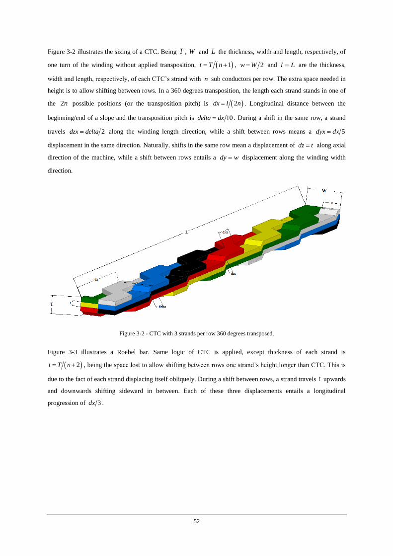
52

Figure 3-2 illustrates the sizing of a CTC. Being T , W and L the thickness, width and length, respectively, of

one turn of the winding without applied transposition, 1t T n , 2w W and l L are the thickness,

width and length, respectively, of each CTC’s strand with n sub conductors per row. The extra space needed in

height is to allow shifting between rows. In a 360 degrees transposition, the length each strand stands in one of

the 2n possible positions (or the transposition pitch) is 2dx l n . Longitudinal distance between the

beginning/end of a slope and the transposition pitch is 10delta dx . During a shift in the same row, a strand

travels 2dzx delta along the winding length direction, while a shift between rows means a 5dyx dx

displacement in the same direction. Naturally, shifts in the same row mean a displacement of dz t along axial

direction of the machine, while a shift between rows entails a dy w displacement along the winding width

direction.

Figure 3-2 - CTC with 3 strands per row 360 degrees transposed.

Figure 3-3 illustrates a Roebel bar. Same logic of CTC is applied, except thickness of each strand is

2t T n , being the space lost to allow shifting between rows one strand’s height longer than CTC. This is

due to the fact of each strand displacing itself obliquely. During a shift between rows, a strand travels t upwards

and downwards shifting sideward in between. Each of these three displacements entails a longitudinal

progression of 3dx .

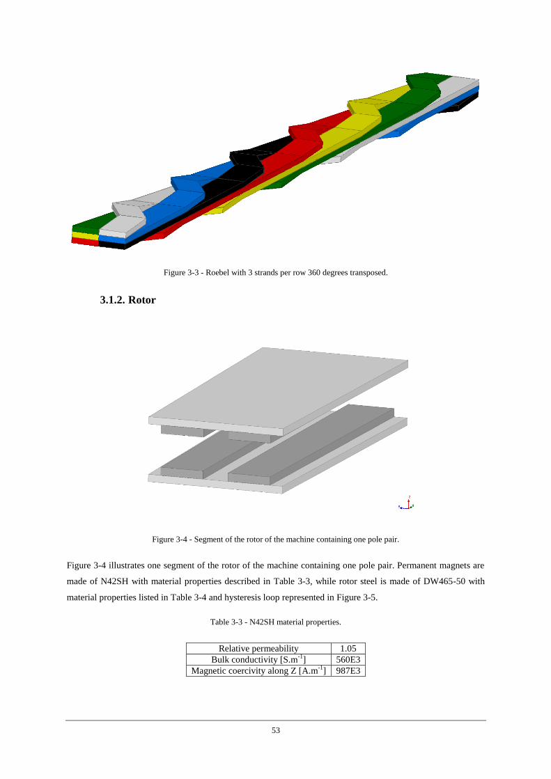
53

Figure 3-3 - Roebel with 3 strands per row 360 degrees transposed.

3.1.2. Rotor

Figure 3-4 - Segment of the rotor of the machine containing one pole pair.

Figure 3-4 illustrates one segment of the rotor of the machine containing one pole pair. Permanent magnets are

made of N42SH with material properties described in Table 3-3, while rotor steel is made of DW465-50 with

material properties listed in Table 3-4 and hysteresis loop represented in Figure 3-5.

Table 3-3 - N42SH material properties.

Relative permeability 1.05

Bulk conductivity [S.m-1

] 560E3

Magnetic coercivity along Z [A.m-1

] 987E3

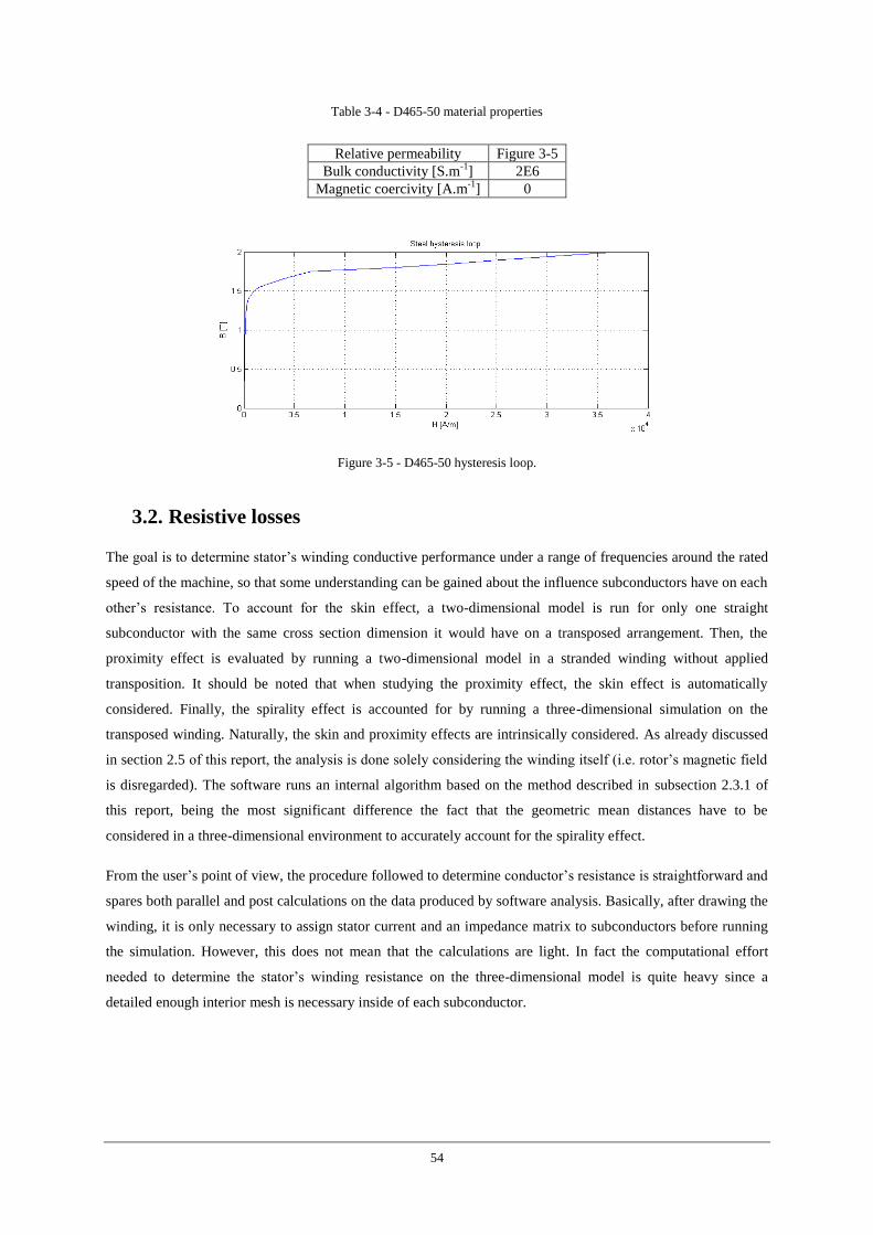
54

Table 3-4 - D465-50 material properties

Relative permeability Figure 3-5

Bulk conductivity [S.m-1

] 2E6

Magnetic coercivity [A.m-1

] 0

Figure 3-5 - D465-50 hysteresis loop.

3.2. Resistive losses

The goal is to determine stator’s winding conductive performance under a range of frequencies around the rated

speed of the machine, so that some understanding can be gained about the influence subconductors have on each

other’s resistance. To account for the skin effect, a two-dimensional model is run for only one straight

subconductor with the same cross section dimension it would have on a transposed arrangement. Then, the

proximity effect is evaluated by running a two-dimensional model in a stranded winding without applied

transposition. It should be noted that when studying the proximity effect, the skin effect is automatically

considered. Finally, the spirality effect is accounted for by running a three-dimensional simulation on the

transposed winding. Naturally, the skin and proximity effects are intrinsically considered. As already discussed

in section 2.5 of this report, the analysis is done solely considering the winding itself (i.e. rotor’s magnetic field

is disregarded). The software runs an internal algorithm based on the method described in subsection 2.3.1 of

this report, being the most significant difference the fact that the geometric mean distances have to be

considered in a three-dimensional environment to accurately account for the spirality effect.

From the user’s point of view, the procedure followed to determine conductor’s resistance is straightforward and

spares both parallel and post calculations on the data produced by software analysis. Basically, after drawing the

winding, it is only necessary to assign stator current and an impedance matrix to subconductors before running

the simulation. However, this does not mean that the calculations are light. In fact the computational effort

needed to determine the stator’s winding resistance on the three-dimensional model is quite heavy since a

detailed enough interior mesh is necessary inside of each subconductor.

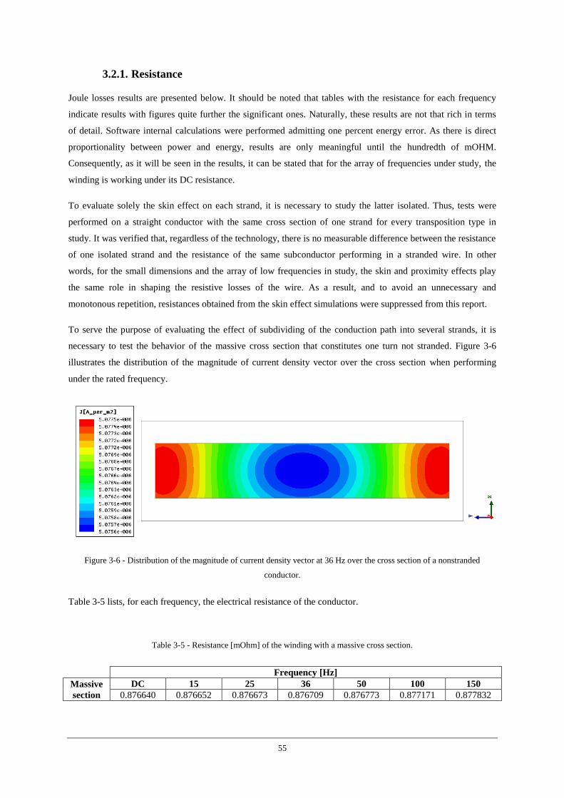
55

3.2.1. Resistance

Joule losses results are presented below. It should be noted that tables with the resistance for each frequency

indicate results with figures quite further the significant ones. Naturally, these results are not that rich in terms

of detail. Software internal calculations were performed admitting one percent energy error. As there is direct

proportionality between power and energy, results are only meaningful until the hundredth of mOHM.

Consequently, as it will be seen in the results, it can be stated that for the array of frequencies under study, the

winding is working under its DC resistance.

To evaluate solely the skin effect on each strand, it is necessary to study the latter isolated. Thus, tests were

performed on a straight conductor with the same cross section of one strand for every transposition type in

study. It was verified that, regardless of the technology, there is no measurable difference between the resistance

of one isolated strand and the resistance of the same subconductor performing in a stranded wire. In other

words, for the small dimensions and the array of low frequencies in study, the skin and proximity effects play

the same role in shaping the resistive losses of the wire. As a result, and to avoid an unnecessary and

monotonous repetition, resistances obtained from the skin effect simulations were suppressed from this report.

To serve the purpose of evaluating the effect of subdividing of the conduction path into several strands, it is

necessary to test the behavior of the massive cross section that constitutes one turn not stranded. Figure 3-6

illustrates the distribution of the magnitude of current density vector over the cross section when performing

under the rated frequency.

Figure 3-6 - Distribution of the magnitude of current density vector at 36 Hz over the cross section of a nonstranded

conductor.

Table 3-5 lists, for each frequency, the electrical resistance of the conductor.

Table 3-5 - Resistance [mOhm] of the winding with a massive cross section.

Frequency [Hz]

Massive

section

DC 15 25 36 50 100 150

0.876640 0.876652 0.876673 0.876709 0.876773 0.877171 0.877832

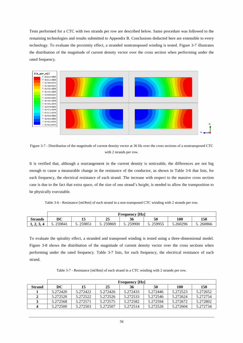
56

Tests performed for a CTC with two strands per row are described below. Same procedure was followed to the

remaining technologies and results submitted to Appendix B. Conclusions deducted here are extensible to every

technology. To evaluate the proximity effect, a stranded nontransposed winding is tested. Figure 3-7 illustrates

the distribution of the magnitude of current density vector over the cross section when performing under the

rated frequency.

Figure 3-7 - Distribution of the magnitude of current density vector at 36 Hz over the cross sections of a nontransposed CTC

with 2 strands per row.

It is verified that, although a rearrangement in the current density is noticeable, the differences are not big

enough to cause a measurable change in the resistance of the conductor, as shown in Table 3-6 that lists, for

each frequency, the electrical resistance of each strand. The increase with respect to the massive cross section

case is due to the fact that extra space, of the size of one strand’s height, is needed to allow the transposition to

be physically executable.

Table 3-6 - Resistance [mOhm] of each strand in a non-transposed CTC winding with 2 strands per row.

Frequency [Hz]

Strands DC 15 25 36 50 100 150

1, 2, 3, 4 5. 259841 5. 259851 5. 259869 5. 259900 5. 259955 5.260296 5. 260866

To evaluate the spirality effect, a stranded and transposed winding is tested using a three-dimensional model.

Figure 3-8 shows the distribution of the magnitude of current density vector over the cross sections when

performing under the rated frequency. Table 3-7 lists, for each frequency, the electrical resistance of each

strand.

Table 3-7 - Resistance [mOhm] of each strand in a CTC winding with 2 strands per row.

Frequency [Hz]

Strand DC 15 25 36 50 100 150

1 5.272420 5.272422 5.272426 5.272433 5.272446 5.272523 5.272652

2 5.272520 5.272522 5.272526 5.272533 5.272546 5.272624 5.272754

3 5.272568 5.272571 5.272575 5.272582 5.272594 5.272672 5.272802

4 5.272500 5.272503 5.272507 5.272514 5.272526 5.272604 5.272734

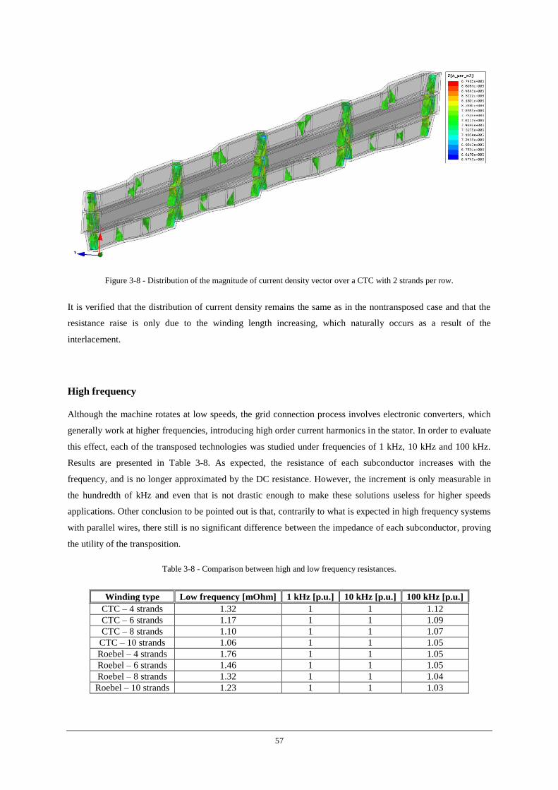
57

Figure 3-8 - Distribution of the magnitude of current density vector over a CTC with 2 strands per row.

It is verified that the distribution of current density remains the same as in the nontransposed case and that the

resistance raise is only due to the winding length increasing, which naturally occurs as a result of the

interlacement.

High frequency

Although the machine rotates at low speeds, the grid connection process involves electronic converters, which

generally work at higher frequencies, introducing high order current harmonics in the stator. In order to evaluate

this effect, each of the transposed technologies was studied under frequencies of 1 kHz, 10 kHz and 100 kHz.

Results are presented in Table 3-8. As expected, the resistance of each subconductor increases with the

frequency, and is no longer approximated by the DC resistance. However, the increment is only measurable in

the hundredth of kHz and even that is not drastic enough to make these solutions useless for higher speeds

applications. Other conclusion to be pointed out is that, contrarily to what is expected in high frequency systems

with parallel wires, there still is no significant difference between the impedance of each subconductor, proving

the utility of the transposition.

Table 3-8 - Comparison between high and low frequency resistances.

Winding type Low frequency [mOhm] 1 kHz [p.u.] 10 kHz [p.u.] 100 kHz [p.u.]

CTC – 4 strands 1.32 1 1 1.12

CTC – 6 strands 1.17 1 1 1.09

CTC – 8 strands 1.10 1 1 1.07

CTC – 10 strands 1.06 1 1 1.05

Roebel – 4 strands 1.76 1 1 1.05

Roebel – 6 strands 1.46 1 1 1.05

Roebel – 8 strands 1.32 1 1 1.04

Roebel – 10 strands 1.23 1 1 1.03

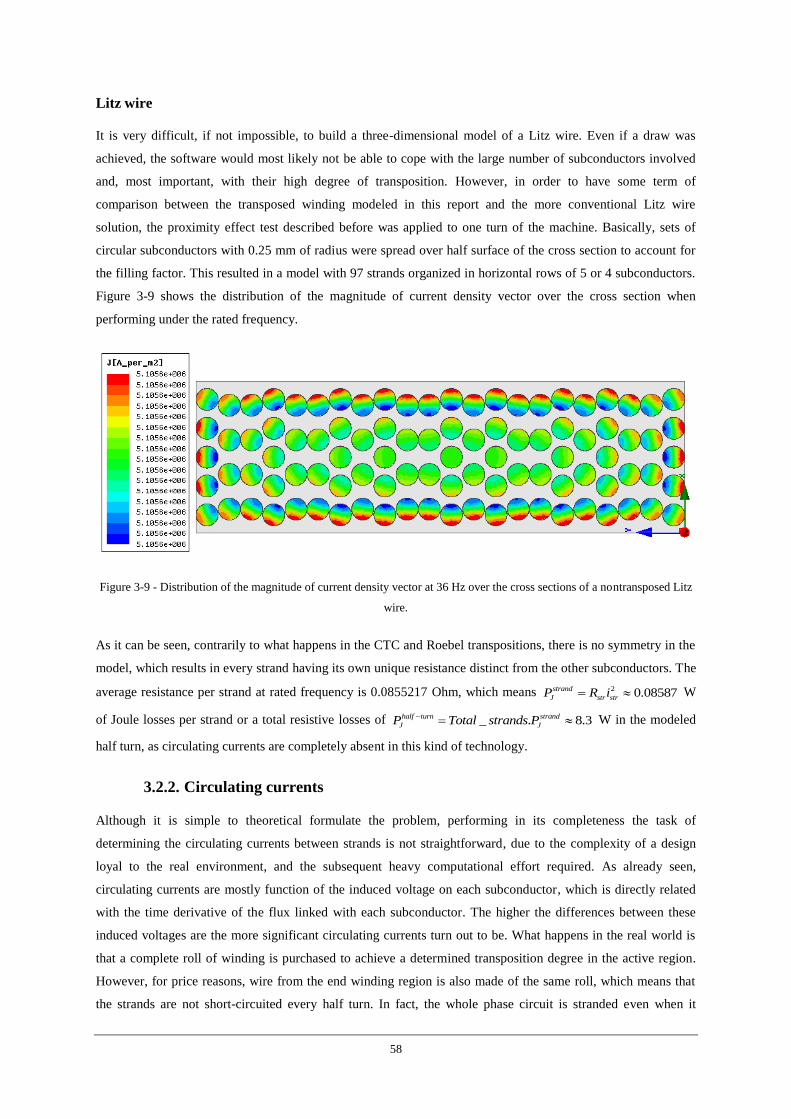
58

Litz wire

It is very difficult, if not impossible, to build a three-dimensional model of a Litz wire. Even if a draw was

achieved, the software would most likely not be able to cope with the large number of subconductors involved

and, most important, with their high degree of transposition. However, in order to have some term of

comparison between the transposed winding modeled in this report and the more conventional Litz wire

solution, the proximity effect test described before was applied to one turn of the machine. Basically, sets of

circular subconductors with 0.25 mm of radius were spread over half surface of the cross section to account for

the filling factor. This resulted in a model with 97 strands organized in horizontal rows of 5 or 4 subconductors.

Figure 3-9 shows the distribution of the magnitude of current density vector over the cross section when

performing under the rated frequency.

Figure 3-9 - Distribution of the magnitude of current density vector at 36 Hz over the cross sections of a nontransposed Litz

wire.

As it can be seen, contrarily to what happens in the CTC and Roebel transpositions, there is no symmetry in the

model, which results in every strand having its own unique resistance distinct from the other subconductors. The

average resistance per strand at rated frequency is 0.0855217 Ohm, which means 2 0.08587strand

J str strP R i W

of Joule losses per strand or a total resistive losses of _ . 8.3half turn strand

J JP Total strands P W in the modeled

half turn, as circulating currents are completely absent in this kind of technology.

3.2.2. Circulating currents

Although it is simple to theoretical formulate the problem, performing in its completeness the task of

determining the circulating currents between strands is not straightforward, due to the complexity of a design

loyal to the real environment, and the subsequent heavy computational effort required. As already seen,

circulating currents are mostly function of the induced voltage on each subconductor, which is directly related

with the time derivative of the flux linked with each subconductor. The higher the differences between these

induced voltages are the more significant circulating currents turn out to be. What happens in the real world is

that a complete roll of winding is purchased to achieve a determined transposition degree in the active region.

However, for price reasons, wire from the end winding region is also made of the same roll, which means that

the strands are not short-circuited every half turn. In fact, the whole phase circuit is stranded even when it

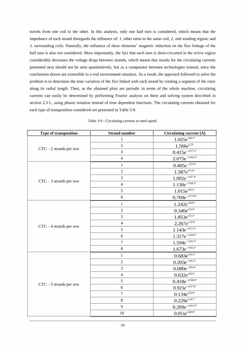
59

travels from one coil to the other. In this analysis, only one half turn is considered, which means that the

impedance of each strand disregards the influence of: 1. other turns in the same coil; 2. end winding region; and

3. surrounding coils. Naturally, the influence of these elements’ magnetic induction on the flux linkage of the

half turn is also not considered. More importantly, the fact that each turn is short-circuited in the active region

considerably decreases the voltage drops between strands, which means that results for the circulating currents

presented next should not be seen quantitatively, but as a comparator between technologies instead, since the

conclusions drawn are extensible to a real environment situation. As a result, the approach followed to solve the

problem is to determine the time variation of the flux linked with each strand by rotating a segment of the rotor

along its radial length. Then, as the obtained plots are periodic in terms of the whole machine, circulating

currents can easily be determined by performing Fourier analysis on them and solving system described in

section 2.3.1., using phasor notation instead of time dependent functions. The circulating currents obtained for

each type of transposition considered are presented in Table 3-9.

Table 3-9 - Circulating currents at rated speed.

Type of transposition Strand number Circulating current [A]

CTC – 2 strands per row

1 58.3º1.025 ie

2 23º1.566 ie

3 157.2º0.415 ie

4 140.4º2.075 ie

CTC – 3 strands per row

1 22.6º0.405 ie

2 12.6º1.587 ie

3 167.4º1.002 ie

4 159.3º1.130 ie

5 30.2º1.015 ie

6 173.9º0.769 ie

CTC – 4 strands per row

1 39.9º1.242 ie

2 33.0º0.340 ie

3 23.5º1.853 ie

4 23.9º2.267 ie

5 151.5º1.143 ie

6 144.9º1.317 ie

7 145.5º1.594 ie

8 165.1º1.673 ie

CTC – 5 strands per row

1 32.2º0.683 ie

2 95.2º0.203 ie

3 19.4º0.080 ie

4 26.0º0.632 ie

5 158.0º0.418 ie

6 157.8º0.921 ie

7 22.9º0.134 ie

8 24.7º0.229 ie

9 161.0º0.269 ie

10 140.8º0.051 ie

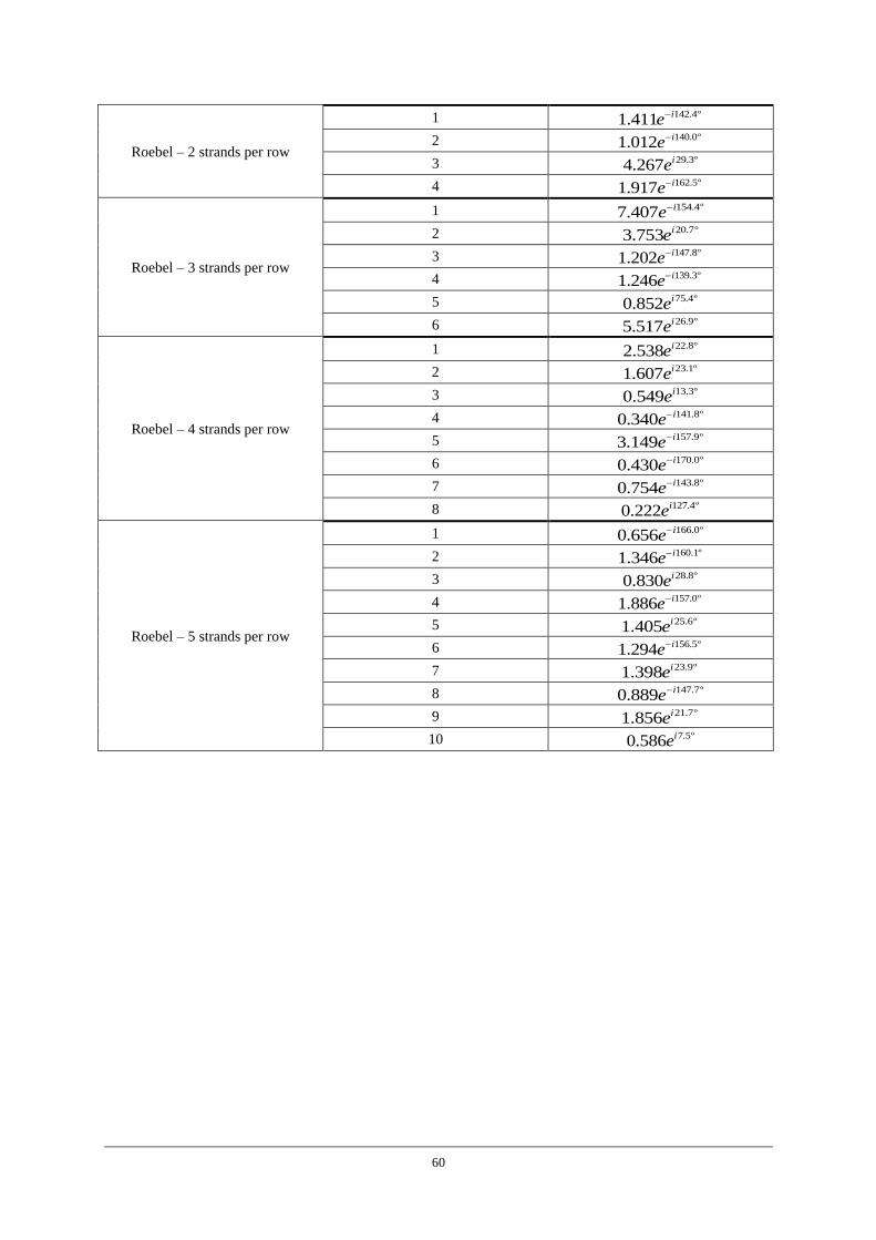
60

Roebel – 2 strands per row

1 142.4º1.411 ie

2 140.0º1.012 ie

3 29.3º4.267 ie

4 162.5º1.917 ie

Roebel – 3 strands per row

1 154.4º7.407 ie

2 20.7º3.753 ie

3 147.8º1.202 ie

4 139.3º1.246 ie

5 75.4º0.852 ie

6 26.9º5.517 ie

Roebel – 4 strands per row

1 22.8º2.538 ie

2 23.1º1.607 ie

3 13.3º0.549 ie

4 141.8º0.340 ie

5 157.9º3.149 ie

6 170.0º0.430 ie

7 143.8º0.754 ie

8 127.4º0.222 ie

Roebel – 5 strands per row

1 166.0º0.656 ie

2 160.1º1.346 ie

3 28.8º0.830 ie

4 157.0º1.886 ie

5 25.6º1.405 ie

6 156.5º1.294 ie

7 23.9º1.398 ie

8 147.7º0.889 ie

9 21.7º1.856 ie

10 7.5º0.586 ie

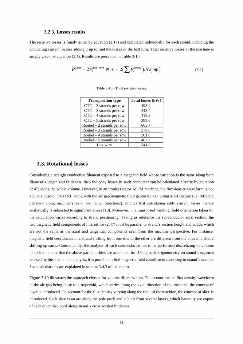
61

3.2.3. Losses results

The resistive losses is finally given by equation (2.17) and calculated individually for each strand, including the

circulating current, before adding it up to find the losses of the half turn. Total resistive losses of the machine is

simply given by equation (3.1). Results are presented in Table 3-10.

2 . . 2 . .Total half turn strand

J J c JP P N n P N mp (3.1)

Table 3-10 - Total resistive losses.

Transposition type Total losses [kW]

CTC – 2 strands per row 498.4

CTC – 3 strands per row 443.4

CTC – 4 strands per row 418.3

CTC – 5 strands per row 399.0

Roebel – 2 strands per row 665.7

Roebel – 3 strands per row 570.0

Roebel – 4 strands per row 501.0

Roebel – 5 strands per row 467.7

Litz wire 341.8

3.3. Rotational losses

Considering a straight conductive filament exposed to a magnetic field whose variation is the same along both

filament’s length and thickness, then the eddy losses in such conductor can be calculated directly by equation

(2.47) along the whole volume. However, in an ironless stator AFPM machine, the flux density waveform is not

a pure sinusoid. This fact, along with the air gap magnetic field geometry exhibiting a 3-D nature (i.e. different

behavior along machine’s axial and radial directions), implies that calculating eddy current losses merely

analytically is subjected to significant errors [10]. Moreover, in a transposed winding, field orientation taken for

the calculation varies according to strand positioning. Taking as reference the subconductor axial section, the

two magnetic field components of interest for (2.47) must be parallel to strand’s section height and width, which

are not the same as the axial and tangential components seen from the machine perspective. For instance,

magnetic field coordinates in a strand shifting from one row to the other are different from the ones in a strand

shifting upwards. Consequently, the analysis of each subconductor has to be performed discretizing its volume

in such a manner that the above particularities are accounted for. Using basic trigonometry on strand’s segment

crossed by the slice under analysis, it is possible to find magnetic field coordinates according to strand’s section.

Such calculations are explained in section 3.4.3 of this report.

Figure 3-10 illustrates the approach chosen for volume discretization. To account for the flux density waveform

in the air gap being close to a trapezoid, which varies along the axial direction of the machine, the concept of

layer is introduced. To account for the flux density varying along the radii of the machine, the concept of slice is

introduced. Each slice is an arc along the pole pitch and is built from several layers, which basically are copies

of each other displaced along strand’s cross section thickness.

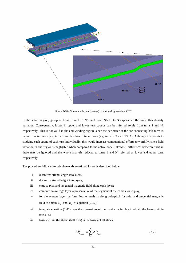
62

Figure 3-10 - Slices and layers (orange) of a strand (green) in a CTC

In the active region, group of turns from 1 to N/2 and from N/2+1 to N experience the same flux density

variation. Consequently, losses in upper and lower turn groups can be inferred solely from turns 1 and N,

respectively. This is not valid in the end winding region, since the perimeter of the arc connecting half turns is

larger in outer turns (e.g. turns 1 and N) than in inner turns (e.g. turns N/2 and N/2+1). Although this points to

studying each strand of each turn individually, this would increase computational efforts unworthily, since field

variation in end region is negligible when compared to the active zone. Likewise, differences between turns in

there may be ignored and the whole analysis reduced to turns 1 and N, referred as lower and upper turn,

respectively.

The procedure followed to calculate eddy rotational losses is described below:

i. discretize strand length into slices;

ii. discretize strand height into layers;

iii. extract axial and tangential magnetic field along each layer;

iv. compute an average layer representative of the segment of the conductor in play;

v. for the average layer, perform Fourier analysis along pole-pitch for axial and tangential magnetic

field to obtain yB and zB of equation (2.47);

vi. integrate equation (2.47) over the dimensions of the conductor in play to obtain the losses within

one slice;

vii. losses within the strand (half turn) is the losses of all slices:

1strand slicek

s

e e

k

P P

(3.2)

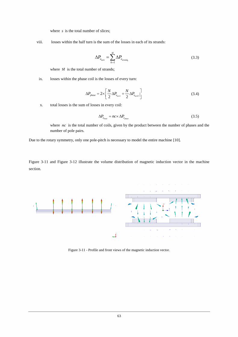
63

where s is the total number of slices;

viii. losses within the half turn is the sum of the losses in each of its strands:

1turn strandk

st

e e

k

P P

(3.3)

where st is the total number of strands;

ix. losses within the phase coil is the losses of every turn:

1

22 2turn turnNphase e e

N NP P P

(3.4)

x. total losses is the sum of losses in every coil:

Total phasee eP nc P (3.5)

where nc is the total number of coils, given by the product between the number of phases and the

number of pole pairs.

Due to the rotary symmetry, only one pole-pitch is necessary to model the entire machine [10].

Figure 3-11 and Figure 3-12 illustrate the volume distribution of magnetic induction vector in the machine

section.

Figure 3-11 - Profile and front views of the magnetic induction vector.

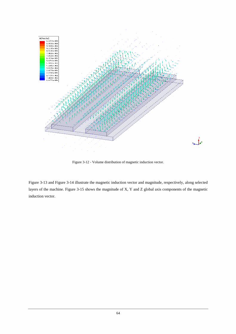
64

Figure 3-12 - Volume distribution of magnetic induction vector.

Figure 3-13 and Figure 3-14 illustrate the magnetic induction vector and magnitude, respectively, along selected

layers of the machine. Figure 3-15 shows the magnitude of X, Y and Z global axis components of the magnetic

induction vector.

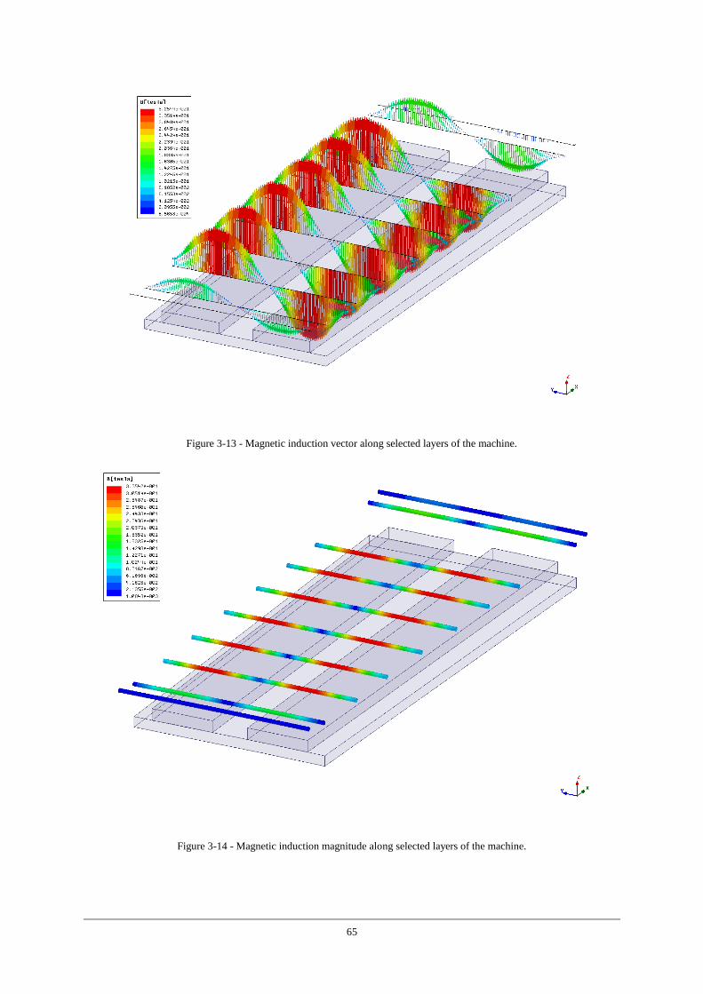
65

Figure 3-13 - Magnetic induction vector along selected layers of the machine.

Figure 3-14 - Magnetic induction magnitude along selected layers of the machine.

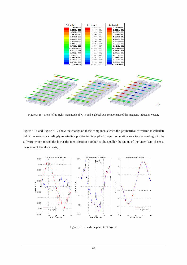
66

Figure 3-15 - From left to right: magnitude of X, Y and Z global axis components of the magnetic induction vector.

Figure 3-16 and Figure 3-17 show the change on those components when the geometrical correction to calculate

field components accordingly to winding positioning is applied. Layer numeration was kept accordingly to the

software which means the lower the identification number is, the smaller the radius of the layer (e.g. closer to

the origin of the global axis).

Figure 3-16 - field components of layer 2.

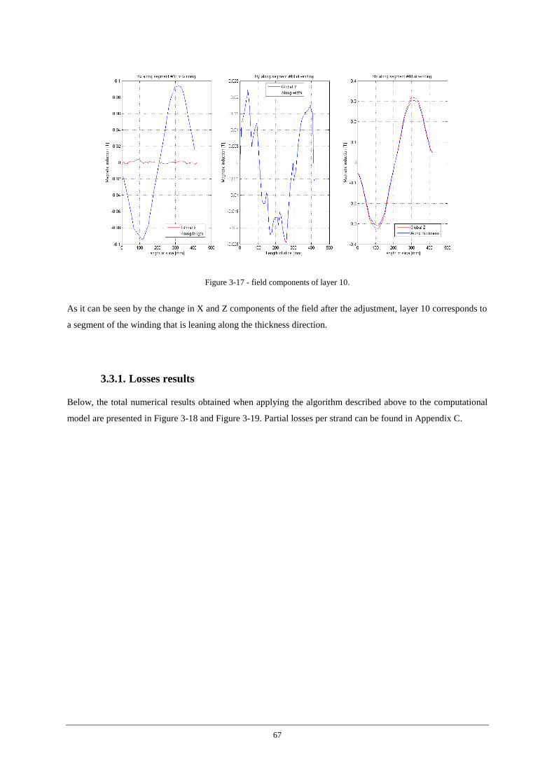
67

Figure 3-17 - field components of layer 10.

As it can be seen by the change in X and Z components of the field after the adjustment, layer 10 corresponds to

a segment of the winding that is leaning along the thickness direction.

3.3.1. Losses results

Below, the total numerical results obtained when applying the algorithm described above to the computational

model are presented in Figure 3-18 and Figure 3-19. Partial losses per strand can be found in Appendix C.

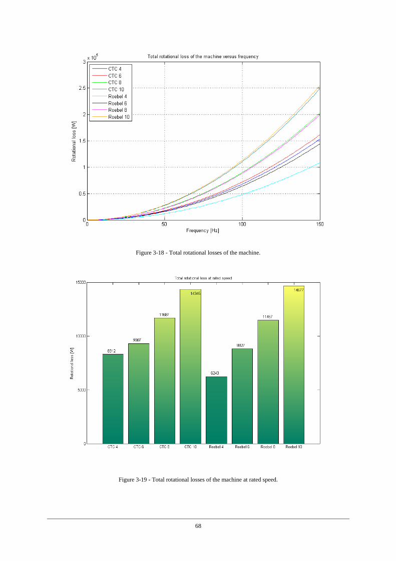
68

Figure 3-18 - Total rotational losses of the machine.

Figure 3-19 - Total rotational losses of the machine at rated speed.

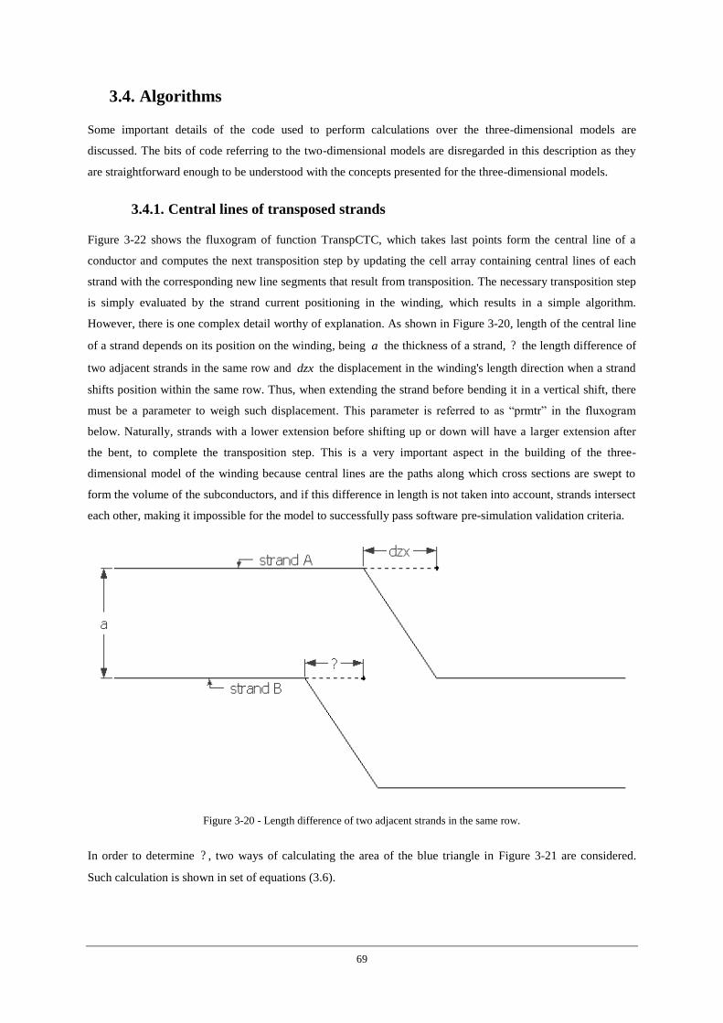
69

3.4. Algorithms

Some important details of the code used to perform calculations over the three-dimensional models are

discussed. The bits of code referring to the two-dimensional models are disregarded in this description as they

are straightforward enough to be understood with the concepts presented for the three-dimensional models.

3.4.1. Central lines of transposed strands

Figure 3-22 shows the fluxogram of function TranspCTC, which takes last points form the central line of a

conductor and computes the next transposition step by updating the cell array containing central lines of each

strand with the corresponding new line segments that result from transposition. The necessary transposition step

is simply evaluated by the strand current positioning in the winding, which results in a simple algorithm.

However, there is one complex detail worthy of explanation. As shown in Figure 3-20, length of the central line

of a strand depends on its position on the winding, being a the thickness of a strand, ? the length difference of

two adjacent strands in the same row and dzx the displacement in the winding's length direction when a strand

shifts position within the same row. Thus, when extending the strand before bending it in a vertical shift, there

must be a parameter to weigh such displacement. This parameter is referred to as “prmtr” in the fluxogram

below. Naturally, strands with a lower extension before shifting up or down will have a larger extension after

the bent, to complete the transposition step. This is a very important aspect in the building of the three-

dimensional model of the winding because central lines are the paths along which cross sections are swept to

form the volume of the subconductors, and if this difference in length is not taken into account, strands intersect

each other, making it impossible for the model to successfully pass software pre-simulation validation criteria.

Figure 3-20 - Length difference of two adjacent strands in the same row.

In order to determine ? , two ways of calculating the area of the blue triangle in Figure 3-21 are considered.

Such calculation is shown in set of equations (3.6).

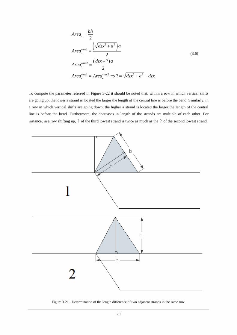
70

2 2

1

2

1 2 2 2

2

2

?

2

?

case

case

case case

bhArea

dzx a aArea

dzx aArea

Area Area dzx a dzx

(3.6)

To compute the parameter referred in Figure 3-22 it should be noted that, within a row in which vertical shifts

are going up, the lower a strand is located the larger the length of the central line is before the bend. Similarly, in

a row in which vertical shifts are going down, the higher a strand is located the larger the length of the central

line is before the bend. Furthermore, the decreases in length of the strands are multiple of each other. For

instance, in a row shifting up, ? of the third lowest strand is twice as much as the ? of the second lowest strand.

Figure 3-21 - Determination of the length difference of two adjacent strands in the same row.

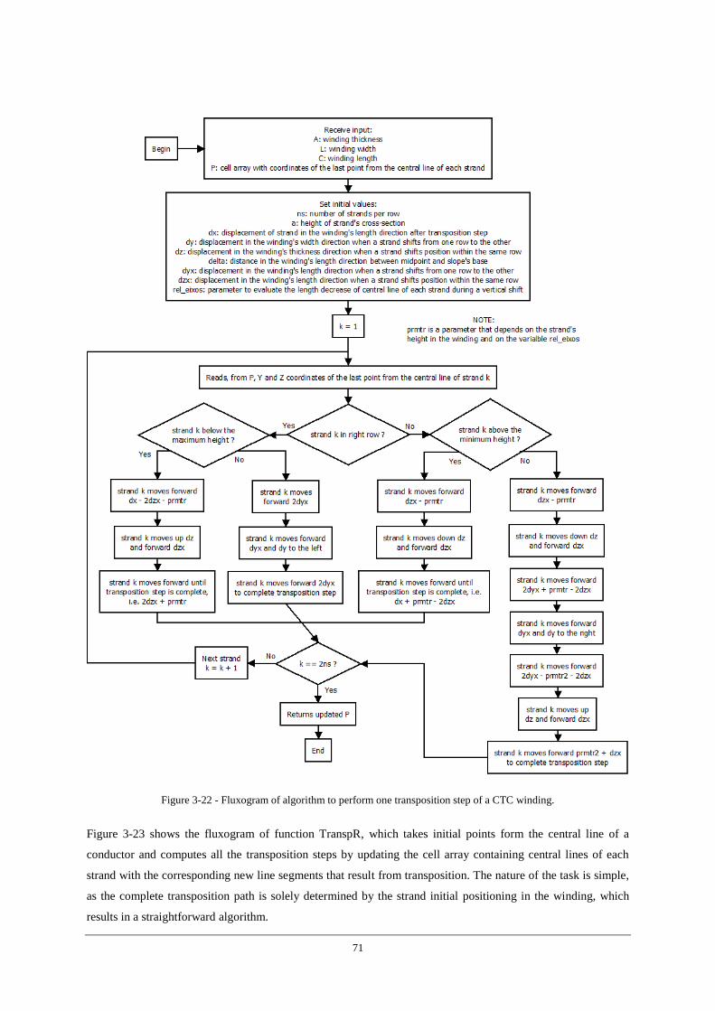
71

Figure 3-22 - Fluxogram of algorithm to perform one transposition step of a CTC winding.

Figure 3-23 shows the fluxogram of function TranspR, which takes initial points form the central line of a

conductor and computes all the transposition steps by updating the cell array containing central lines of each

strand with the corresponding new line segments that result from transposition. The nature of the task is simple,

as the complete transposition path is solely determined by the strand initial positioning in the winding, which

results in a straightforward algorithm.

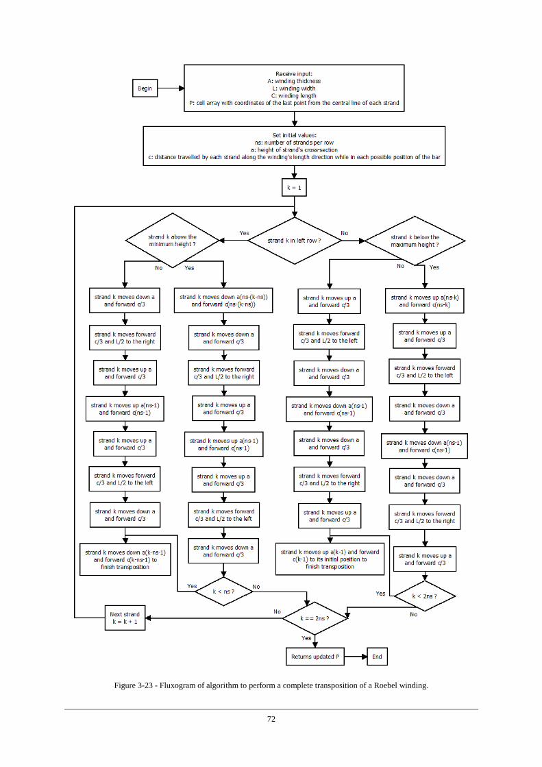
72

Figure 3-23 - Fluxogram of algorithm to perform a complete transposition of a Roebel winding.

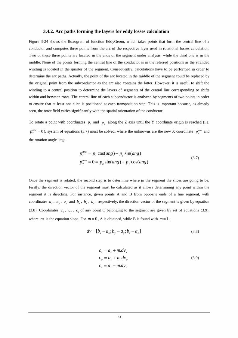
73

3.4.2. Arc paths forming the layers for eddy losses calculation

Figure 3-24 shows the fluxogram of function EddyGeom, which takes points that form the central line of a

conductor and computes three points from the arc of the respective layer used in rotational losses calculation.

Two of these three points are located in the ends of the segment under analysis, while the third one is in the

middle. None of the points forming the central line of the conductor is in the referred positions as the stranded

winding is located in the quarter of the segment. Consequently, calculations have to be performed in order to

determine the arc paths. Actually, the point of the arc located in the middle of the segment could be replaced by

the original point from the subconductor as the arc also contains the latter. However, it is useful to shift the

winding to a central position to determine the layers of segments of the central line corresponding to shifts

within and between rows. The central line of each subconductor is analyzed by segments of two points in order

to ensure that at least one slice is positioned at each transposition step. This is important because, as already

seen, the rotor field varies significantly with the spatial orientation of the conductor.

To rotate a point with coordinates xp and

yp along the Z axis until the Y coordinate origin is reached (i.e.

0new

yp ), system of equations (3.7) must be solved, where the unknowns are the new X coordinate new

xp and

the rotation angle ang .

cos( ) sin( )

0 sin( ) cos( )

new

x x y

new

y x y

p p ang p ang

p p ang p ang

(3.7)

Once the segment is rotated, the second step is to determine where in the segment the slices are going to be.

Firstly, the direction vector of the segment must be calculated as it allows determining any point within the

segment it is directing. For instance, given points A and B from opposite ends of a line segment, with

coordinates xa ,

ya , za and

xb , yb ,

zb , respectively, the direction vector of the segment is given by equation

(3.8). Coordinates xc ,

yc , zc of any point C belonging to the segment are given by set of equations (3.9),

where m is the equation slope. For 0m , A is obtained, while B is found with 1m .

[ ; ; ]x x y y z zdv b a b a b a (3.8)

.

.

.

x x x

y y y

z z z

c a m dv

c a m dv

c a m dv

(3.9)

74

Figure 3-24 - Fluxogram of algorithm followed to build layers used in eddy losses calculation.

75

Following the same logic, positioning of the first slice (i.e. the one nearest to the first point of the segment) can

be determined by solving system of equations (3.10), with the equation slope m also as an unknown and where

ds is the slice discretization step. After knowing the coordinates of the first slice and the equation slope, the

computation of the coordinates of the remaining slices is straightforward.

1

1

2 21 1

.

.

slice

x x x

slice

z z z

slice slice

x x z z

p p m dv

p p m dv

p p p p ds

(3.10)

Although slightly more complex, the computation of the coordinates of the layers follows the same principles

described for the slices. It should be noted that layer's central point position is firstly determined as belonging to

the segment and only then is rotated to its true out of the segment place. First layer is computed using the exact

same approach as in system of equations (3.10), only replacing ds by the layer discretization step dl . Then the

procedure is repeated, replacing ds by half of strand's thickness, in order to find the maximum height for the

layer. Using both equations slopes that result from the solution of the two previous systems, it is possible to

determine layers positioning within the subconductor. Finally, it is necessary to rotate the found coordinates

+90º and -90º. Coordinates are given accordingly to the global coordinate system. However, in order to perform

rotations that will take layers to their true positions the reference for rotation must be the axis of the slice.

Consequently, the procedure to correctly achieve rotations is firstly to perform a translation by taking the point

to near the origin of the global coordinate system (i.e. as far from it as it originally is from the slice); then,

perform the rotation following the method described by set of equations (3.7); and finally perform the inverse

translation in order to take the point back to its original position near the subconductor.

3.4.3. Rotational losses calculation

Figure 3-25 shows the fluxogram of function RotLosses, which takes parameters specifying the type of winding

and the dimensions of the machine to compute the total eddy losses, as well as the losses within each strand on

both lower and upper turns. Active region central lines are drawn using function TranspCTC or TranspR,

depending on the transposition type, while the link between active and end region is achieved as follows. The

available data for this purpose regards the model with a non-transposed winding, made of a massive cross

section, thus a relation had to be found between the line linking both regions in that situation and the position of

central lines of each strand in the transposed coil. Set of equations (3.11) shows the coordinates of the six points

from the central line of a massive cross section winding that form the end winding region. As illustrated in

Figure 3-26, points 1, 2 and 3 form the inner end region, while points 4, 5 and 6 correspond to the outer end

region. Naturally, points 1 and 4 are also part of the active region. It should be noted that the coordinates of

these points are given already considering the true position of the coil, which is rotated along the Z axis by w ,

i.e. a quarter of the angle of one segment of the machine containing one pole pair .

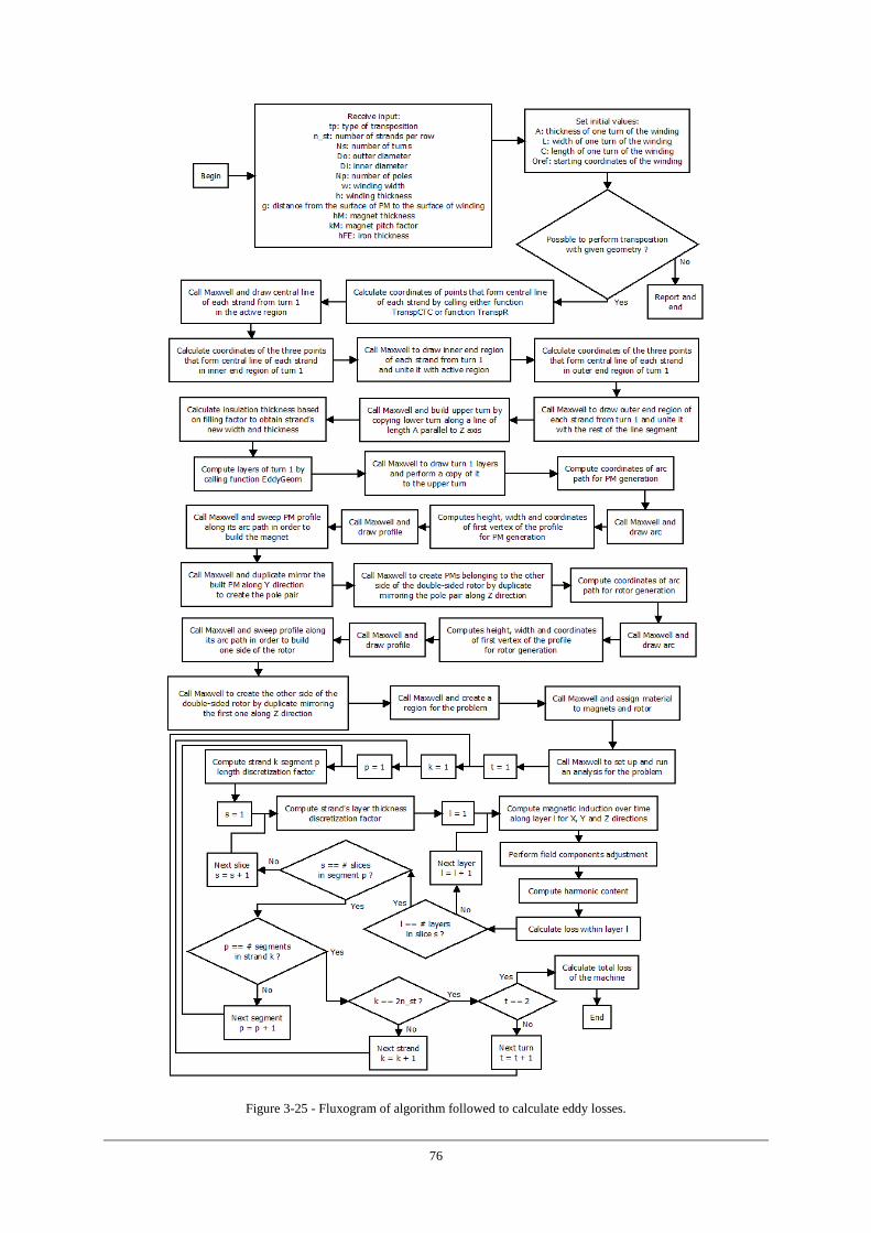
76

Figure 3-25 - Fluxogram of algorithm followed to calculate eddy losses.

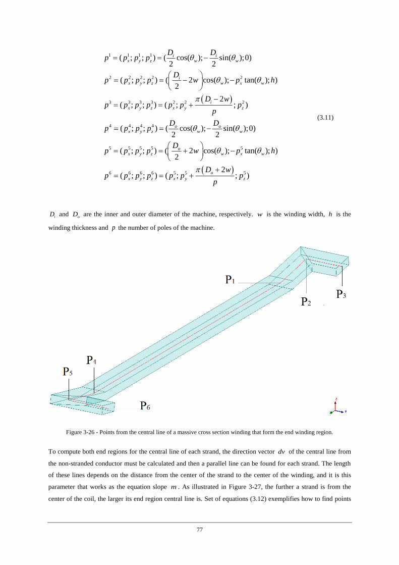
77

1 1 1 1

2 2 2 2 2

3 3 3 3 2 2 2

4 4 4 4

5 5 5 5

( ; ; ) ( cos( ); sin( );0)2 2

( ; ; ) ( 2 cos( ); tan( ); )2

2( ; ; ) ( ; ; )

( ; ; ) ( cos( ); sin( );0)2 2

( ; ; ) ( 22

i ix y z w w

ix y z w x w

i

x y z x y z

o ox y z w w

ox y z

D Dp p p p

Dp p p p w p h

D wp p p p p p p

p

D Dp p p p

Dp p p p w

5

6 6 6 6 5 5 5

cos( ); tan( ); )

2( ; ; ) ( ; ; )

w x w

o

x y z x y z

p h

D wp p p p p p p

p

(3.11)

iD and oD are the inner and outer diameter of the machine, respectively. w is the winding width, h is the

winding thickness and p the number of poles of the machine.

Figure 3-26 - Points from the central line of a massive cross section winding that form the end winding region.

To compute both end regions for the central line of each strand, the direction vector dv of the central line from

the non-stranded conductor must be calculated and then a parallel line can be found for each strand. The length

of these lines depends on the distance from the center of the strand to the center of the winding, and it is this

parameter that works as the equation slope m . As illustrated in Figure 3-27, the further a strand is from the

center of the coil, the larger its end region central line is. Set of equations (3.12) exemplifies how to find points

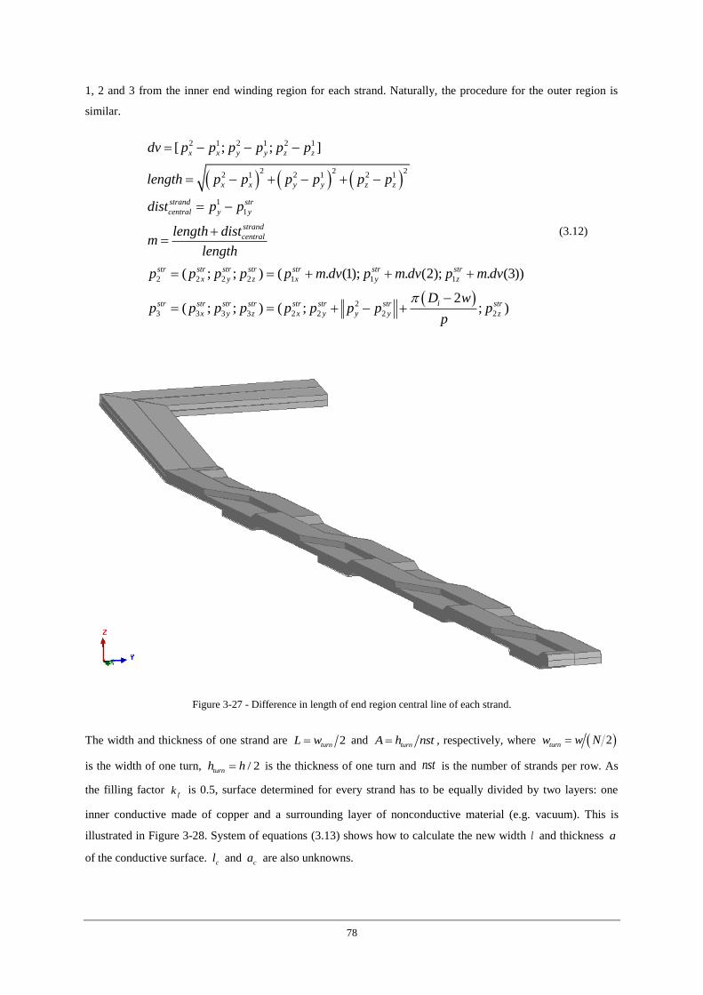
78

1, 2 and 3 from the inner end winding region for each strand. Naturally, the procedure for the outer region is

similar.

2 1 2 1 2 1

2 2 22 1 2 1 2 1

1

1

2 2 2 2 1 1 1

3

[ ; ; ]

( ; ; ) ( . (1); . (2); . (3))

x x y y z z

x x y y z z

strand str

central y y

strand

central

str str str str str str str

x y z x y z

st

dv p p p p p p

length p p p p p p

dist p p

length distm

length

p p p p p m dv p m dv p m dv

p

2

3 3 3 2 2 2 2

2( ; ; ) ( ; ; )

ir str str str str str str str

x y z x y y y z

D wp p p p p p p p

p

(3.12)

Figure 3-27 - Difference in length of end region central line of each strand.

The width and thickness of one strand are 2turnL w and turnA h nst , respectively, where 2turnw w N

is the width of one turn, / 2turnh h is the thickness of one turn and nst is the number of strands per row. As

the filling factor fk is 0.5, surface determined for every strand has to be equally divided by two layers: one

inner conductive made of copper and a surrounding layer of nonconductive material (e.g. vacuum). This is

illustrated in Figure 3-28. System of equations (3.13) shows how to calculate the new width l and thickness a

of the conductive surface. cl and ca are also unknowns.

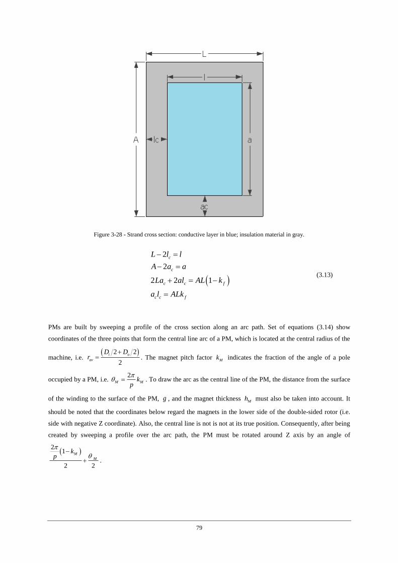
79

Figure 3-28 - Strand cross section: conductive layer in blue; insulation material in gray.

2

2

2 2 1

c

c

c c f

c c f

L l l

A a a

La al AL k

a l ALk

(3.13)

PMs are built by sweeping a profile of the cross section along an arc path. Set of equations (3.14) show

coordinates of the three points that form the central line arc of a PM, which is located at the central radius of the

machine, i.e. 2 2

2

i o

av

D Dr

. The magnet pitch factor

Mk indicates the fraction of the angle of a pole

occupied by a PM, i.e. 2

M Mkp

. To draw the arc as the central line of the PM, the distance from the surface

of the winding to the surface of the PM, g , and the magnet thickness Mh must also be taken into account. It

should be noted that the coordinates below regard the magnets in the lower side of the double-sided rotor (i.e.

side with negative Z coordinate). Also, the central line is not is not at its true position. Consequently, after being

created by sweeping a profile over the arc path, the PM must be rotated around Z axis by an angle of

2

1

2 2

M

M

kp

.

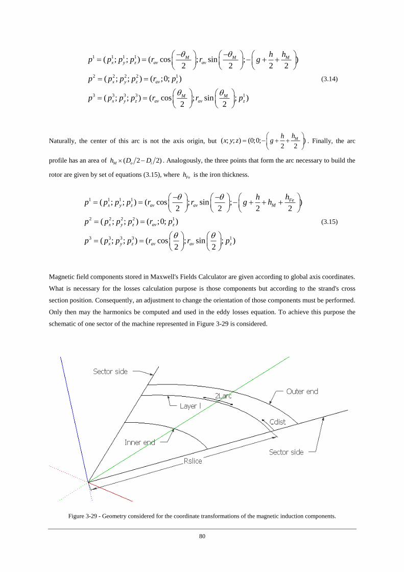
80

1 1 1 1

2 2 2 2 1

3 3 3 3 1

( ; ; ) ( cos ; sin ; )2 2 2 2

( ; ; ) ( ;0; )

( ; ; ) ( cos ; sin ; )2 2

M M Mx y z av av

x y z av z

M Mx y z av av z

hhp p p p r r g

p p p p r p

p p p p r r p

(3.14)

Naturally, the center of this arc is not the axis origin, but ( ; ; ) (0;0; )2 2

Mhhx y z g

. Finally, the arc

profile has an area of ( 2 2)M o ih D D . Analogously, the three points that form the arc necessary to build the

rotor are given by set of equations (3.15), where Feh is the iron thickness.

1 1 1 1

2 2 2 2 1

3 3 3 3 1

( ; ; ) ( cos ; sin ; )2 2 2 2

( ; ; ) ( ;0; )

( ; ; ) ( cos ; sin ; )2 2

Fex y z av av M

x y z av z

x y z av av z

hhp p p p r r g h

p p p p r p

p p p p r r p

(3.15)

Magnetic field components stored in Maxwell's Fields Calculator are given according to global axis coordinates.

What is necessary for the losses calculation purpose is those components but according to the strand's cross

section position. Consequently, an adjustment to change the orientation of those components must be performed.

Only then may the harmonics be computed and used in the eddy losses equation. To achieve this purpose the

schematic of one sector of the machine represented in Figure 3-29 is considered.

Figure 3-29 - Geometry considered for the coordinate transformations of the magnetic induction components.

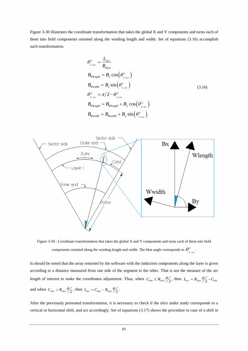
81

Figure 3-30 illustrates the coordinate transformation that takes the global X and Y components and turns each of

them into field components oriented along the winding length and width. Set of equations (3.16) accomplish

such transformation.

cos

sin

2

cos

sin

G arc

G arc

G arc

G arc G arc

G arc

G arc

x arc

slice

x

Wlength x

x

Wwidth x

y x

y

Wlength Wlength y

y

Wwidth Wwidth y

L

R

B B

B B

B B B

B B B

(3.16)

Figure 3-30 - Coordinate transformation that takes the global X and Y components and turns each of them into field

components oriented along the winding length and width. The blue angle corresponds to G arc

x

.

Is should be noted that the array returned by the software with the induction components along the layer is given

according to a distance measured from one side of the segment to the other. That is not the measure of the arc

length of interest to make the coordinates adjustment. Thus, when 2dist sliceC R , then

2arc slice distL R C

and when 2dist sliceC R , then

2arc dist sliceL C R .

After the previously presented transformation, it is necessary to check if the slice under study corresponds to a

vertical or horizontal shift, and act accordingly. Set of equations (3.17) shows the procedure in case of a shift in

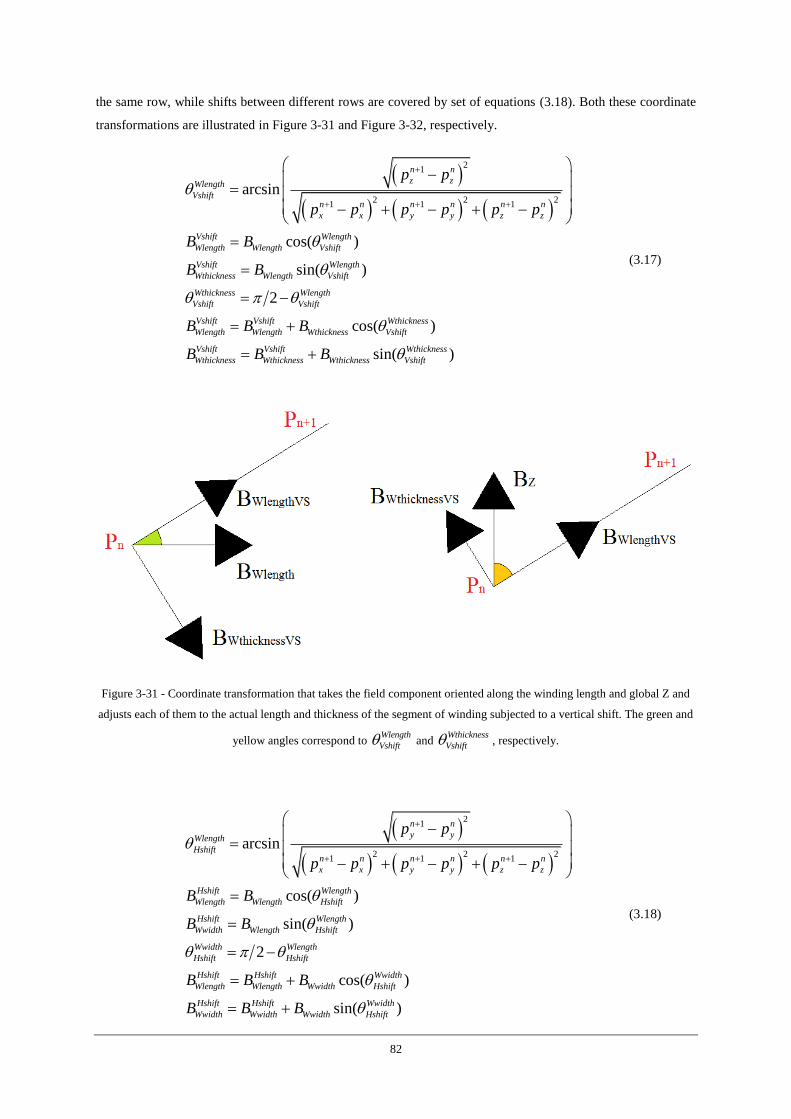
82

the same row, while shifts between different rows are covered by set of equations (3.18). Both these coordinate

transformations are illustrated in Figure 3-31 and Figure 3-32, respectively.

21

2 2 21 1 1

arcsin

cos( )

sin( )

2

n n

z zWlength

Vshiftn n n n n n

x x y y z z

Vshift Wlength

Wlength Wlength Vshift

Vshift Wlength

Wthickness Wlength Vshift

Wthickness Wlength

Vshift Vshift

Wlen

p p

p p p p p p

B B

B B

B

cos( )

sin( )

Vshift Vshift Wthickness

gth Wlength Wthickness Vshift

Vshift Vshift Wthickness

Wthickness Wthickness Wthickness Vshift

B B

B B B

(3.17)

Figure 3-31 - Coordinate transformation that takes the field component oriented along the winding length and global Z and

adjusts each of them to the actual length and thickness of the segment of winding subjected to a vertical shift. The green and

yellow angles correspond to Wlength

Vshift and Wthickness

Vshift , respectively.

21

2 2 21 1 1

arcsin

cos( )

sin( )

2

n n

y yWlength

Hshiftn n n n n n

x x y y z z

Hshift Wlength

Wlength Wlength Hshift

Hshift Wlength

Wwidth Wlength Hshift

Wwidth Wlength

Hshift Hshift

Hshif

Wlength

p p

p p p p p p

B B

B B

B

cos( )

sin( )

t Hshift Wwidth

Wlength Wwidth Hshift

Hshift Hshift Wwidth

Wwidth Wwidth Wwidth Hshift

B B

B B B

(3.18)

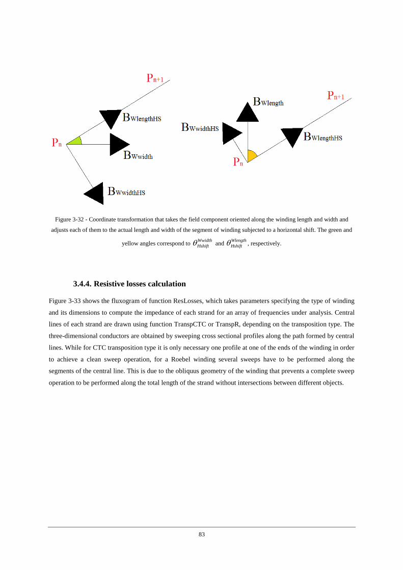
83

Figure 3-32 - Coordinate transformation that takes the field component oriented along the winding length and width and

adjusts each of them to the actual length and width of the segment of winding subjected to a horizontal shift. The green and

yellow angles correspond to Wwidth

Hshift and Wlength

Hshift , respectively.

3.4.4. Resistive losses calculation

Figure 3-33 shows the fluxogram of function ResLosses, which takes parameters specifying the type of winding

and its dimensions to compute the impedance of each strand for an array of frequencies under analysis. Central

lines of each strand are drawn using function TranspCTC or TranspR, depending on the transposition type. The

three-dimensional conductors are obtained by sweeping cross sectional profiles along the path formed by central

lines. While for CTC transposition type it is only necessary one profile at one of the ends of the winding in order

to achieve a clean sweep operation, for a Roebel winding several sweeps have to be performed along the

segments of the central line. This is due to the obliquus geometry of the winding that prevents a complete sweep

operation to be performed along the total length of the strand without intersections between different objects.

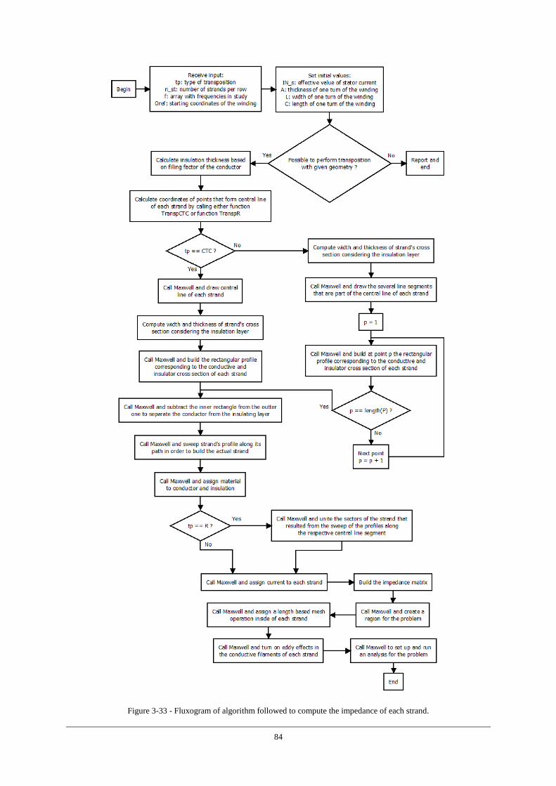
84

Figure 3-33 - Fluxogram of algorithm followed to compute the impedance of each strand.

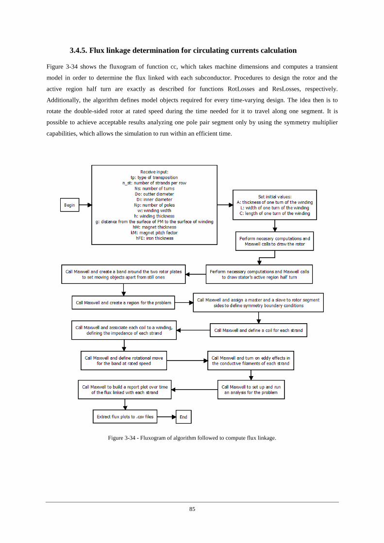
85

3.4.5. Flux linkage determination for circulating currents calculation

Figure 3-34 shows the fluxogram of function cc, which takes machine dimensions and computes a transient

model in order to determine the flux linked with each subconductor. Procedures to design the rotor and the

active region half turn are exactly as described for functions RotLosses and ResLosses, respectively.

Additionally, the algorithm defines model objects required for every time-varying design. The idea then is to

rotate the double-sided rotor at rated speed during the time needed for it to travel along one segment. It is

possible to achieve acceptable results analyzing one pole pair segment only by using the symmetry multiplier

capabilities, which allows the simulation to run within an efficient time.

Figure 3-34 - Fluxogram of algorithm followed to compute flux linkage.

86

87

Chapter 4

4. Conclusions

This chapter is aimed at detailing overall conclusions of the thesis as well as presenting future work

perspectives.

88

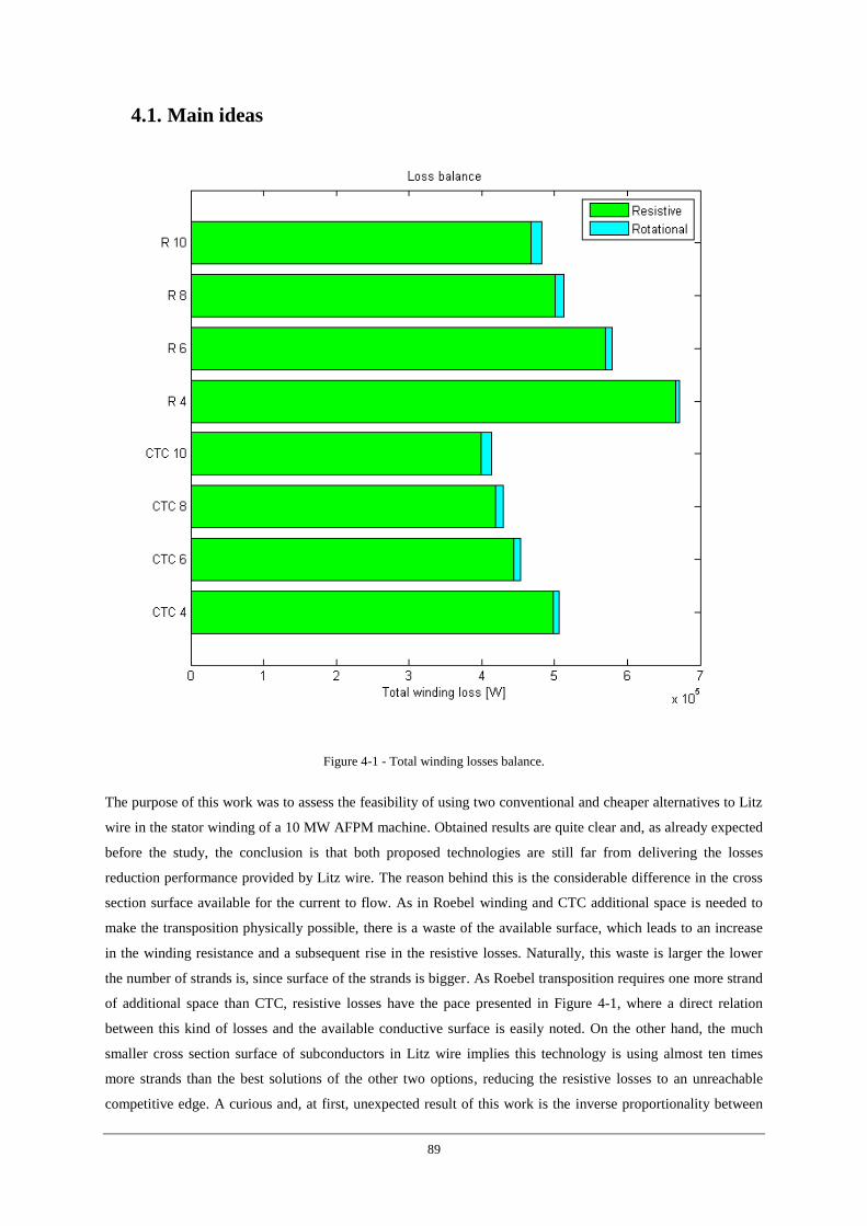
89

4.1. Main ideas

Figure 4-1 - Total winding losses balance.

The purpose of this work was to assess the feasibility of using two conventional and cheaper alternatives to Litz

wire in the stator winding of a 10 MW AFPM machine. Obtained results are quite clear and, as already expected

before the study, the conclusion is that both proposed technologies are still far from delivering the losses

reduction performance provided by Litz wire. The reason behind this is the considerable difference in the cross

section surface available for the current to flow. As in Roebel winding and CTC additional space is needed to

make the transposition physically possible, there is a waste of the available surface, which leads to an increase

in the winding resistance and a subsequent rise in the resistive losses. Naturally, this waste is larger the lower

the number of strands is, since surface of the strands is bigger. As Roebel transposition requires one more strand

of additional space than CTC, resistive losses have the pace presented in Figure 4-1, where a direct relation

between this kind of losses and the available conductive surface is easily noted. On the other hand, the much

smaller cross section surface of subconductors in Litz wire implies this technology is using almost ten times

more strands than the best solutions of the other two options, reducing the resistive losses to an unreachable

competitive edge. A curious and, at first, unexpected result of this work is the inverse proportionality between

90

the number of strands and obtained rotational losses, as illustrated in Figure 4-1. It would seem logic to think

that if subdividing the conductor in several subconductors serves the purpose of reducing eddy current effects,

then the more intense that division is, the sharpest rotational losses reduction would be. It is true that using a

stranded conductor instead of a massive one provides better rotational losses performance, as it will be shown

further in this section. However, since a stranded wire is built from several parallel circuits, transposition has to

be performed in order that the induced EMFs in all parallel conductors are equalized, consequently reducing

circulating currents. This fact implies that the available conductive surface is larger in the cases with more sub

conductors, thus increasing rotational losses. Another fact that may contribute to this increase with the number

of strands is that, as explained in section 3.4.3 of this report, when the conductor is transposed, the changes in its

dimensions orientation along the transposition path may cause the components of the flux that contribute to the

rotational losses to mutual increase each other. Understandably, components of the flux may also align in a way

they cancel each other out. The number of winding direction changes is proportional to the number of strands,

and what these results indicate is that, in this two specific types of transposition, most direction changes in

transposition steps cause the flux components to increase their effective value for the rotational losses. Figure

4-1 indicates that, at the end, an apparent random pace is followed by total winding losses, which implies a

balance must be made between resistive and rotational losses in order to find the best solution for given

dimensions. Nevertheless, it is not clear that the process of subdividing winding conductors is work that pays off

in terms of total winding losses reduction. Table 4-1 shows the gain in transposing the winding weighting it

against the case with a massive cross section, which dimensions are 973.5 mm of length and 19.15 mm2 of

available conductive surface. Recalling its resistance, already presented in section 3.2.1, a total resistive losses

of 339.9 kW is found. Same approach described in section 3.3 of this report was followed for the no stranded

conductor and 42.9 kW was obtained for the rotational losses.

Table 4-1 - Comparison between transpositions weighted against no transposed winding.

Winding type Surface [%] Length [%] Resistive losses [p.u.] Rotational losses [p.u.]

Massive cross section 100 100 1 1

CTC – 4 strands 66.7 100.23 1.46 0.19

CTC – 6 strands 75 100.3 1.30 0.22

CTC – 8 strands 80 100.34 1.23 0.27

CTC – 10 strands 83.3 100.37 1.17 0.33

Roebel – 4 strands 50 100.03 1.96 0.15

Roebel – 6 strands 60 100.03 1.68 0.21

Roebel – 8 strands 66.7 100.03 1.47 0.27

Roebel – 10 strands 71.4 100.04 1.38 0.34

An issue that should be discussed is the advantages of using a tridimensional simulation. It should be pondered

if it is possible or not to achieve similar results with a two-dimensional model and if the computational effort

spent is worthwhile. Table D-1 of Appendix D gives a general idea of the computational effort required to run

each of the model analysis used in this report, in terms of used memory and completion time. Rotational losses

calculation in AFPM machines is usually described in the literature (e.g. [10] and [15]) as a two-dimensional

problem. However, following the same method in a three-dimensional environment provides more accurate

results not only due to the flux density varying along the radii of the machine, but also because it is not possible

91

to account for the magnetic flux variation within a transposed coil using a two-dimensional model. In terms of

resistive losses, there is now no doubt similar results could be achieved merely by recurring to the analytical

expression that gives the resistance of a conductor. This happens because of the low frequencies under study.

Basically, skin, proximity and spirality effects are unnoticeable and the impedance of the winding is simply only

a function of its dimensions. However, the extremely heavy three-dimensional simulation run was not in vain

since self and mutual inductances of the subconductors were needed for circulating currents determination.

Highly dependent on the geometry, this parameter requires a three-dimensional model. Even considering that

including circulating currents in the resistive losses calculation is not a crucial step, as shown in Table 4-2, this

is not a reason to underrate the method because it can still be used to determine how big transposition angle has

to bring the losses to a desired level.

Table 4-2 - Weight of circulating currents in Joule losses.

Transposition type Circulating currents contribution [%]

CTC – 4 strands 0.17

CTC – 6 strands 0.21

CTC – 8 strands 0.78

CTC – 10 strands 0.11

Roebel – 4 strands 0.52

Roebel – 6 strands 3.17

Roebel – 8 strands 0.85

Roebel – 10 strands 0.87

4.2. What remains to be done

An analysis of circulating currents in a stranded but no transposed winding is clearly missing in this report to

assess about how worth 360 degrees transposition is. Furthermore, and although the type of generator under

consideration is a low frequency machine, it would be interesting to have performed calculations under

frequencies that make skin, proximity and spirality effects measurable. This would not only allow concluding

about the usefulness of Roebel winding and CTC for other applications, but would also provide proof or rebuttal

about the general consideration that by stranding a tubular conductor the skin effect is reduced as the number of

strands is increased, providing the number of subconductors is greater than seven [16]. But even with that, the

work developed in this study would be far from being complete. In fact, it only represents a small first step to

the final ambition of creating an algorithm that outputs the cheapest solution for winding technology given a

maximum value of accepted losses. It is safe to say that this study serves as solid background to accomplish the

referred big final task because principles that support these algorithms were built over a parameterized basis. In

other words, the exact same scripts may be used to perform the same kind of calculations for other machines

with different dimensions. Several future works may follow, for instance to study different types of transposition

that makes use of the fact that the field varies over the radii of the machine, or integrate an economic analysis

with winding losses calculation to evaluate the maximum degree before deciding which type of winding will be

part of the stator.

92

The resistance limited eddy losses in the stator of an AFPM machine may be experimentally determined by

measuring the difference in input shaft powers of the AFPM machine at the same speed, first with the stator in,

and then by replacing it with a dummy stator (no conductors). The dummy stator has the same dimensions and

surface finish as the real stator and is meant to keep the windage losses the same. The shaft of the tested

prototype and the shaft of the driving machine are coupled together via a torque meter. The stator is positioned

in the middle of the two rotor discs with the outer end ring mounted on the outside supporting frame. Initially,

the prototype with the coreless stator placed in it is driven by a variable speed motor for a number of different

speeds and the corresponding torque measurements are taken. Replacing the real stator with a dummy one, the

tests are repeated for the same speeds. Using the logic expressed in equation (2.22), the difference of the torques

multiplied by the speed gives the eddy current losses. The eddy losses due to eddy-circulating currents in the

windings can also be determined by measuring the difference of input shaft powers, first with all the parallel

circuits connected and then with disconnected parallel circuits [4]. For a number of reasons related with the

priority on the access to the prototype of the machine, it was not possible to complete the experimental test by

the time this report was submitted. However, a wooden stator, whose scheme is illustrated in Appendix E, was

already built and practical results are expected to be included in a future paper. At the moment, the next steps

are upgrading the shaft line, setting the torque sensor, and replacing the real stator.

93

References [1]. [Online] http://www.ieee.org/portal/site/emergingtech/techindex.jsp?techId=260

[2]. [Online] http://www.offshorewindenergy.org/

[3]. Z. Zhang, A. Matveev, S. Øvrebø, R. Nilssen, A. Nysveen, State of the Art in Generator Technology

for Offshore Wind Energy Conversion Systems, IEEE, 2011.

[4]. J. Gieras, RJ. Wang, M. Kamper, Axial Flux Permanent Magnet Brushless Machines, Springer, Second

Edition, 2008.

[5]. R. Bargallo, Finite Elements for Electrical Engineering, Electrical Engineering Department of

Universitat Politécnica de Catalunya, 2006.

[6]. J. Faria, Electromagnetic Foundations of Electrical Engineering, Wiley, First Edition, 2008.

[7]. AE. Fitzgerald, C. Kingsley, S. Umans, Electric Machinery, McGraw-Hill, Sixth Edition, 2003.

[8]. AE. Kennelly, FA. Laws, PH. Pierce, Experimental Researches on Skin Effect in Conductors, AIEE,

1915.

[9]. S. Berleze, R. Robert, Skin and Proximity Effects in Nonmagnetic Conductors, IEEE, 2003.

[10]. R. Wang, MJ. Kamper, Evaluation of Eddy Current Losses in Axial Flux Permanent Magnet Machine

with an Ironless Stator, IEEE, 2002.

[11]. K. Takahashi, M. Takahashi, M. Sato, Calculation Method for Strand Current Distributions in

Armature Winding of a Turbine Generator, IEEE, 2003.

[12]. SJ. Salon, Finite Element Analysis of Electrical Machines, Kluwer Academic Publishers, First Edition,

1995.

[13]. M. Chapman, T. Kaffenberger, A. Matveev, P. Olsen, Developments Relating to Litz Wire in the

Insulation Systems of Generators for Renewable Energies, IEEE, 2011.

[14]. RL. Stoll, R. Hindmarsh, Reduction of local eddy-current losses in turbogenerator stator windings

using composite subconductors, Proc. IEE, 1976.

[15]. GW. Carter, The Electromagnetic Field in its Engineering Aspects, Longmans, Third Edition, 1958.

[16]. HB. Dwight, Skin Effect and Proximity Effect in Tubular Conductors, Transactions AIEE, 1922.

94

95

Appendix A

Formulas from vector analysis

96

97

A.1 Gradient

The gradient vector field of a scalar function 1( ,..., )nf x x is defined as the unique vector field whose dot

product with any unit vector at each point is the directional derivative of the function along that unit vector. In a

rectangular coordinate system, the gradient is the vector field whose components are the partial derivatives of

f :

1

1

... n

n

f ff e e

x x

ie are the orthogonal unit vectors pointing in the coordinate directions.

In terms of physical interpretation, the variation in space of any quantity can be represented by a slope and the

gradient represents the steepness and direction of that slope.

A.2 Divergence

Being , ,x y z a system of Cartesian coordinates in 3-dimensional Euclidean space, and , ,i j k the corresponding

basis of unit vectors, then the divergence of a continuously differentiable vector field F Ui V j Wk is

equal to the scalar-valued function:

U V W

Fx y z

In terms of physical interpretation, the divergence represents the volume density of the outward flux of a vector

field from an infinitesimal volume around a given point.

A.3 Curl

Expanded in Cartesian coordinates, the curl of a continuously differentiable vector field F composed of

, ,x y zF F F is equal to the vector field:

x y z

i j k

Fx y z

F F F

, ,i j k are the unit vectors for the , ,x y z axes, respectively. This expands as follows:

98

y yx xz z

F FF FF FF i j k

y z z x x y

In terms of physical interpretation, at every point in the field F , the curl is represented by a vector. The length

and direction of this vector characterize the rotation at that point. The direction of the curl is the axis of rotation,

as determined by the right-hand rule, and the magnitude of the curl is the magnitude of rotation.

A.4 Gauss’ theorem

The Gauss’ theorem relates the volume integral of the divergence of a vector field D over a volume V to the

surface integral over a closed surface VS , bounding a region of volume V , of the dot product of D and the

outward unit normal 0n .

0

VV S

DdV D n dS

A.5 Stokes’ theorem

The Stokes’ theorem relates the surface integral of the curl of a vector field A over a surface S in Euclidean

three-space to the line integral of the vector field over its boundary s :

s

S

S s

A n dS A ds

99

Appendix B

Resistive losses: resistance

100

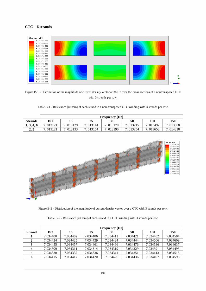
101

CTC – 6 strands

Figure B-1 - Distribution of the magnitude of current density vector at 36 Hz over the cross sections of a nontransposed CTC

with 3 strands per row.

Table B-1 - Resistance [mOhm] of each strand in a non-transposed CTC winding with 3 strands per row.

Frequency [Hz]

Strands DC 15 25 36 50 100 150

1, 3, 4, 6 7. 013121 7. 013129 7. 013144 7. 013170 7. 013215 7. 013497 7. 013968

2, 5 7. 013121 7. 013133 7. 013154 7. 013190 7. 013254 7. 013653 7. 014318

Figure B-2 - Distribution of the magnitude of current density vector over a CTC with 3 strands per row.

Table B-2 - Resistance [mOhm] of each strand in a CTC winding with 3 strands per row.

Frequency [Hz]

Strand DC 15 25 36 50 100 150

1 7.034400 7.034402 7.034406 7.034411 7.034421 7.034482 7.034584

2 7.034424 7.034425 7.034429 7.034434 7.034444 7.034506 7.034609

3 7.034455 7.034457 7.034461 7.034466 7.034476 7.034536 7.034637

4 7.034309 7.034311 7.034314 7.034319 7.034329 7.034391 7.034493

5 7.034330 7.034332 7.034336 7.034341 7.034351 7.034413 7.034515

6 7.034415 7.034417 7.034420 7.034426 7.034436 7.034497 7.034598

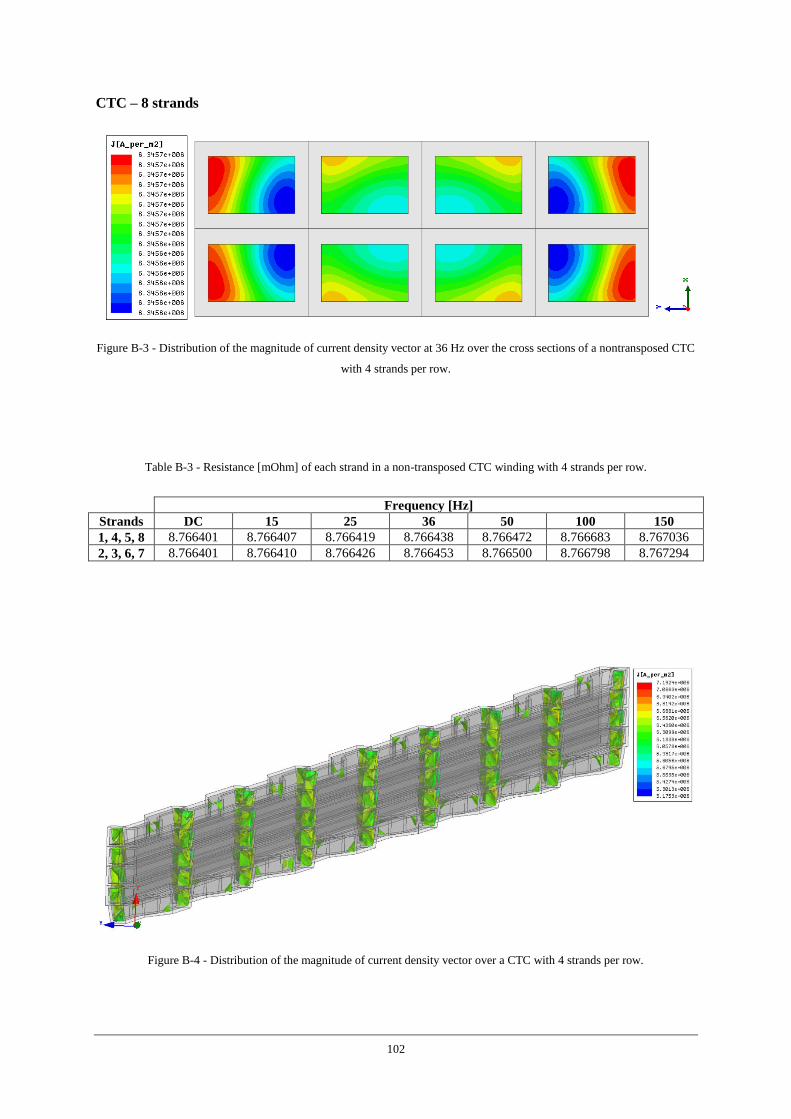
102

CTC – 8 strands

Figure B-3 - Distribution of the magnitude of current density vector at 36 Hz over the cross sections of a nontransposed CTC

with 4 strands per row.

Table B-3 - Resistance [mOhm] of each strand in a non-transposed CTC winding with 4 strands per row.

Frequency [Hz]

Strands DC 15 25 36 50 100 150

1, 4, 5, 8 8.766401 8.766407 8.766419 8.766438 8.766472 8.766683 8.767036

2, 3, 6, 7 8.766401 8.766410 8.766426 8.766453 8.766500 8.766798 8.767294

Figure B-4 - Distribution of the magnitude of current density vector over a CTC with 4 strands per row.

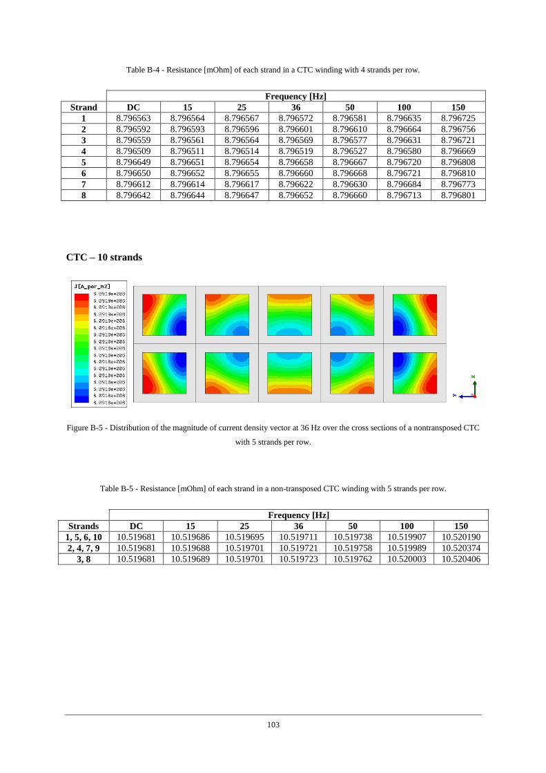
103

Table B-4 - Resistance [mOhm] of each strand in a CTC winding with 4 strands per row.

Frequency [Hz]

Strand DC 15 25 36 50 100 150

1 8.796563 8.796564 8.796567 8.796572 8.796581 8.796635 8.796725

2 8.796592 8.796593 8.796596 8.796601 8.796610 8.796664 8.796756

3 8.796559 8.796561 8.796564 8.796569 8.796577 8.796631 8.796721

4 8.796509 8.796511 8.796514 8.796519 8.796527 8.796580 8.796669

5 8.796649 8.796651 8.796654 8.796658 8.796667 8.796720 8.796808

6 8.796650 8.796652 8.796655 8.796660 8.796668 8.796721 8.796810

7 8.796612 8.796614 8.796617 8.796622 8.796630 8.796684 8.796773

8 8.796642 8.796644 8.796647 8.796652 8.796660 8.796713 8.796801

CTC – 10 strands

Figure B-5 - Distribution of the magnitude of current density vector at 36 Hz over the cross sections of a nontransposed CTC

with 5 strands per row.

Table B-5 - Resistance [mOhm] of each strand in a non-transposed CTC winding with 5 strands per row.

Frequency [Hz]

Strands DC 15 25 36 50 100 150

1, 5, 6, 10 10.519681 10.519686 10.519695 10.519711 10.519738 10.519907 10.520190

2, 4, 7, 9 10.519681 10.519688 10.519701 10.519721 10.519758 10.519989 10.520374

3, 8 10.519681 10.519689 10.519701 10.519723 10.519762 10.520003 10.520406

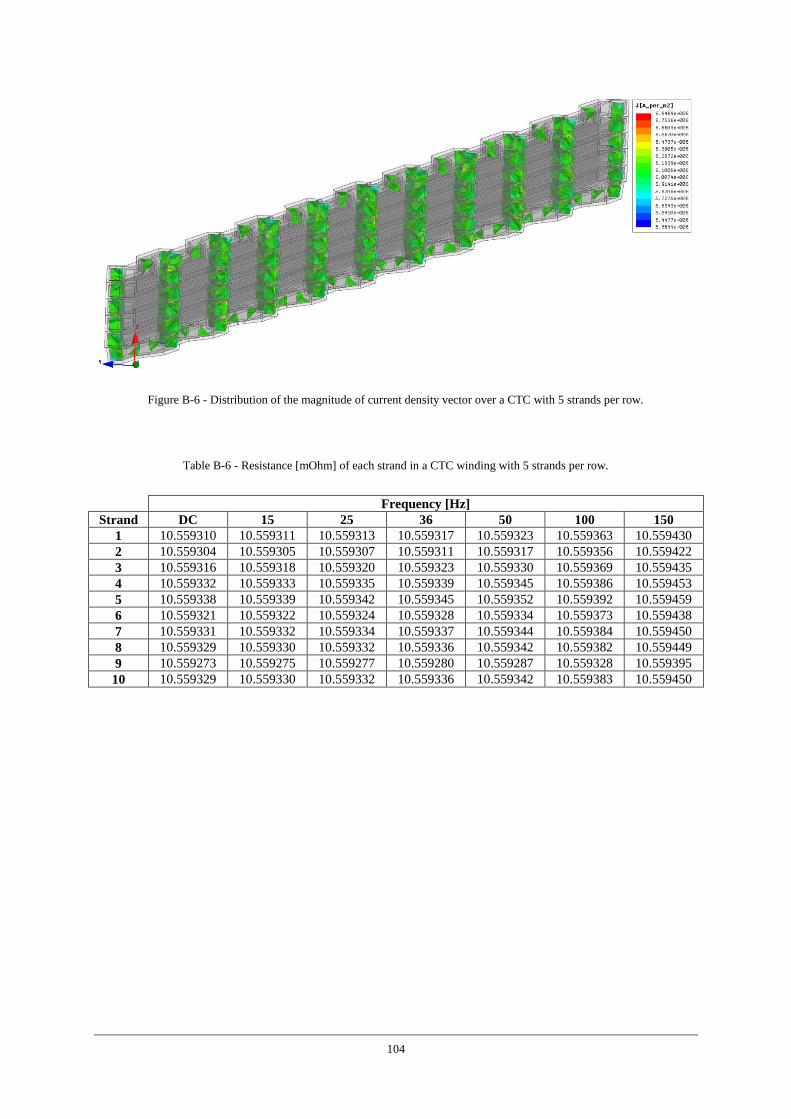
104

Figure B-6 - Distribution of the magnitude of current density vector over a CTC with 5 strands per row.

Table B-6 - Resistance [mOhm] of each strand in a CTC winding with 5 strands per row.

Frequency [Hz]

Strand DC 15 25 36 50 100 150

1 10.559310 10.559311 10.559313 10.559317 10.559323 10.559363 10.559430

2 10.559304 10.559305 10.559307 10.559311 10.559317 10.559356 10.559422

3 10.559316 10.559318 10.559320 10.559323 10.559330 10.559369 10.559435

4 10.559332 10.559333 10.559335 10.559339 10.559345 10.559386 10.559453

5 10.559338 10.559339 10.559342 10.559345 10.559352 10.559392 10.559459

6 10.559321 10.559322 10.559324 10.559328 10.559334 10.559373 10.559438

7 10.559331 10.559332 10.559334 10.559337 10.559344 10.559384 10.559450

8 10.559329 10.559330 10.559332 10.559336 10.559342 10.559382 10.559449

9 10.559273 10.559275 10.559277 10.559280 10.559287 10.559328 10.559395

10 10.559329 10.559330 10.559332 10.559336 10.559342 10.559383 10.559450

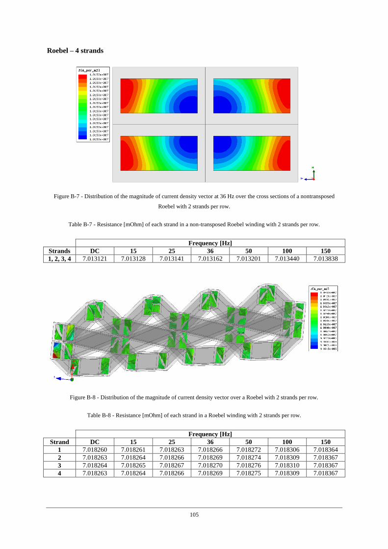
105

Roebel – 4 strands

Figure B-7 - Distribution of the magnitude of current density vector at 36 Hz over the cross sections of a nontransposed

Roebel with 2 strands per row.

Table B-7 - Resistance [mOhm] of each strand in a non-transposed Roebel winding with 2 strands per row.

Frequency [Hz]

Strands DC 15 25 36 50 100 150

1, 2, 3, 4 7.013121 7.013128 7.013141 7.013162 7.013201 7.013440 7.013838

Figure B-8 - Distribution of the magnitude of current density vector over a Roebel with 2 strands per row.

Table B-8 - Resistance [mOhm] of each strand in a Roebel winding with 2 strands per row.

Frequency [Hz]

Strand DC 15 25 36 50 100 150

1 7.018260 7.018261 7.018263 7.018266 7.018272 7.018306 7.018364

2 7.018263 7.018264 7.018266 7.018269 7.018274 7.018309 7.018367

3 7.018264 7.018265 7.018267 7.018270 7.018276 7.018310 7.018367

4 7.018263 7.018264 7.018266 7.018269 7.018275 7.018309 7.018367

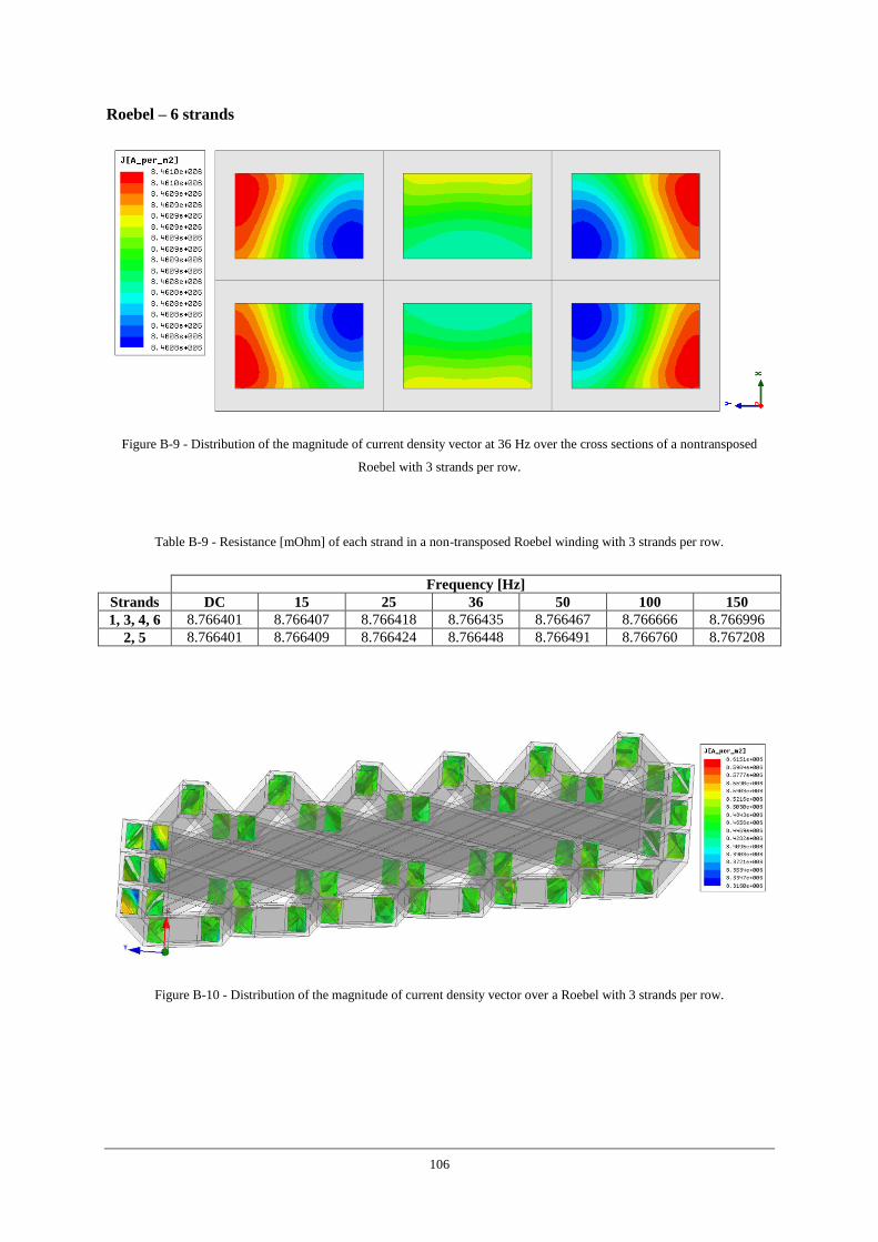
106

Roebel – 6 strands

Figure B-9 - Distribution of the magnitude of current density vector at 36 Hz over the cross sections of a nontransposed

Roebel with 3 strands per row.

Table B-9 - Resistance [mOhm] of each strand in a non-transposed Roebel winding with 3 strands per row.

Frequency [Hz]

Strands DC 15 25 36 50 100 150

1, 3, 4, 6 8.766401 8.766407 8.766418 8.766435 8.766467 8.766666 8.766996

2, 5 8.766401 8.766409 8.766424 8.766448 8.766491 8.766760 8.767208

Figure B-10 - Distribution of the magnitude of current density vector over a Roebel with 3 strands per row.

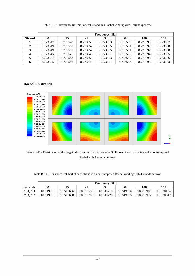
107

Table B-10 - Resistance [mOhm] of each strand in a Roebel winding with 3 strands per row.

Frequency [Hz]

Strand DC 15 25 36 50 100 150

1 8.773547 8.773548 8.773550 8.773553 8.773559 8.773596 8.773657

2 8.773549 8.773550 8.773552 8.773555 8.773561 8.773597 8.773658

3 8.773549 8.773550 8.773552 8.773555 8.773561 8.773597 8.773658

4 8.773545 8.773546 8.773548 8.773551 8.773557 8.773594 8.773655

5 8.773547 8.773548 8.773550 8.773553 8.773559 8.773595 8.773656

6 8.773545 8.773546 8.773548 8.773551 8.773557 8.773593 8.773653

Roebel – 8 strands

Figure B-11 - Distribution of the magnitude of current density vector at 36 Hz over the cross sections of a nontransposed

Roebel with 4 strands per row.

Table B-11 - Resistance [mOhm] of each strand in a non-transposed Roebel winding with 4 strands per row.

Frequency [Hz]

Strands DC 15 25 36 50 100 150

1, 4, 5, 8 10.519681 10.519686 10.519695 10.519710 10.519736 10.519900 10.520174

2, 3, 6, 7 10.519681 10.519688 10.519700 10.519720 10.519755 10.519977 10.520347

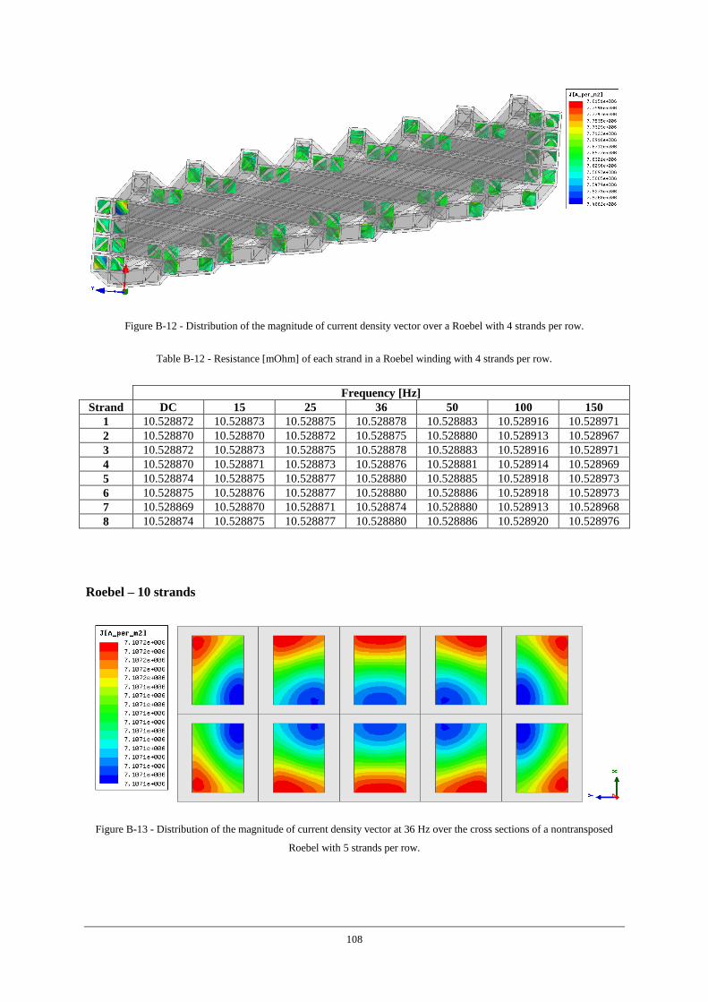
108

Figure B-12 - Distribution of the magnitude of current density vector over a Roebel with 4 strands per row.

Table B-12 - Resistance [mOhm] of each strand in a Roebel winding with 4 strands per row.

Frequency [Hz]

Strand DC 15 25 36 50 100 150

1 10.528872 10.528873 10.528875 10.528878 10.528883 10.528916 10.528971

2 10.528870 10.528870 10.528872 10.528875 10.528880 10.528913 10.528967

3 10.528872 10.528873 10.528875 10.528878 10.528883 10.528916 10.528971

4 10.528870 10.528871 10.528873 10.528876 10.528881 10.528914 10.528969

5 10.528874 10.528875 10.528877 10.528880 10.528885 10.528918 10.528973

6 10.528875 10.528876 10.528877 10.528880 10.528886 10.528918 10.528973

7 10.528869 10.528870 10.528871 10.528874 10.528880 10.528913 10.528968

8 10.528874 10.528875 10.528877 10.528880 10.528886 10.528920 10.528976

Roebel – 10 strands

Figure B-13 - Distribution of the magnitude of current density vector at 36 Hz over the cross sections of a nontransposed

Roebel with 5 strands per row.

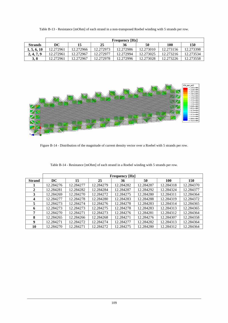
109

Table B-13 - Resistance [mOhm] of each strand in a non-transposed Roebel winding with 5 strands per row.

Frequency [Hz]

Strands DC 15 25 36 50 100 150

1, 5, 6, 10 12.272961 12.272966 12.272973 12.272986 12.273010 12.273156 12.273398

2, 4, 7, 9 12.272961 12.272967 12.272977 12.272994 12.273025 12.273216 12.273534

3, 8 12.272961 12.272967 12.272978 12.272996 12.273028 12.273226 12.273558

Figure B-14 - Distribution of the magnitude of current density vector over a Roebel with 5 strands per row.

Table B-14 - Resistance [mOhm] of each strand in a Roebel winding with 5 strands per row.

Frequency [Hz]

Strand DC 15 25 36 50 100 150

1 12.284276 12.284277 12.284279 12.284282 12.284287 12.284318 12.284370

2 12.284281 12.284282 12.284284 12.284287 12.284292 12.284324 12.284377

3 12.284269 12.284270 12.284272 12.284275 12.284280 12.284311 12.284364

4 12.284277 12.284278 12.284280 12.284283 12.284288 12.284319 12.284372

5 12.284273 12.284274 12.284276 12.284278 12.284283 12.284314 12.284365

6 12.284273 12.284273 12.284275 12.284278 12.284283 12.284313 12.284365

7 12.284270 12.284271 12.284273 12.284276 12.284281 12.284312 12.284364

8 12.284265 12.284266 12.284268 12.284271 12.284276 12.284307 12.284358

9 12.284271 12.284272 12.284274 12.284277 12.284282 12.284313 12.284364

10 12.284270 12.284271 12.284272 12.284275 12.284280 12.284312 12.284364

110

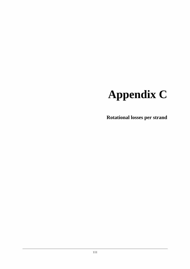
111

Appendix C

Rotational losses per strand

112

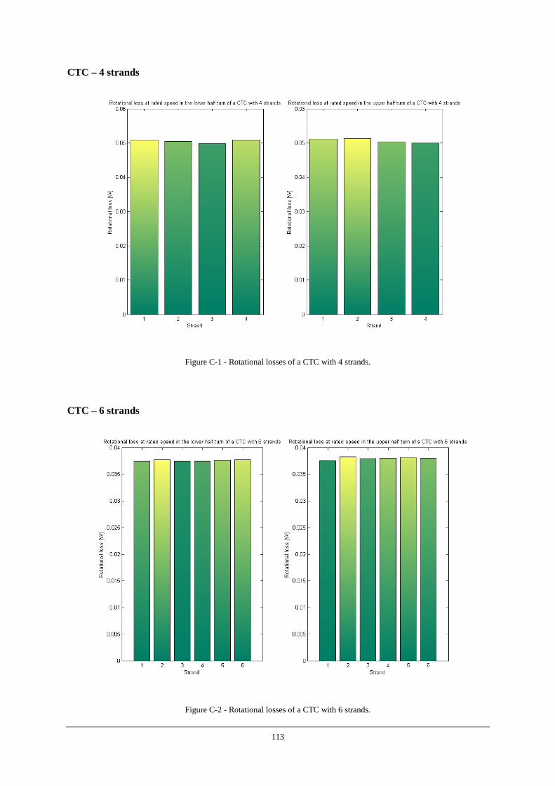
113

CTC – 4 strands

Figure C-1 - Rotational losses of a CTC with 4 strands.

CTC – 6 strands

Figure C-2 - Rotational losses of a CTC with 6 strands.

114

CTC – 8 strands

Figure C-3 - Rotational losses of a CTC with 8 strands.

CTC – 10 strands

Figure C-4 - Rotational losses of a CTC with 10 strands.

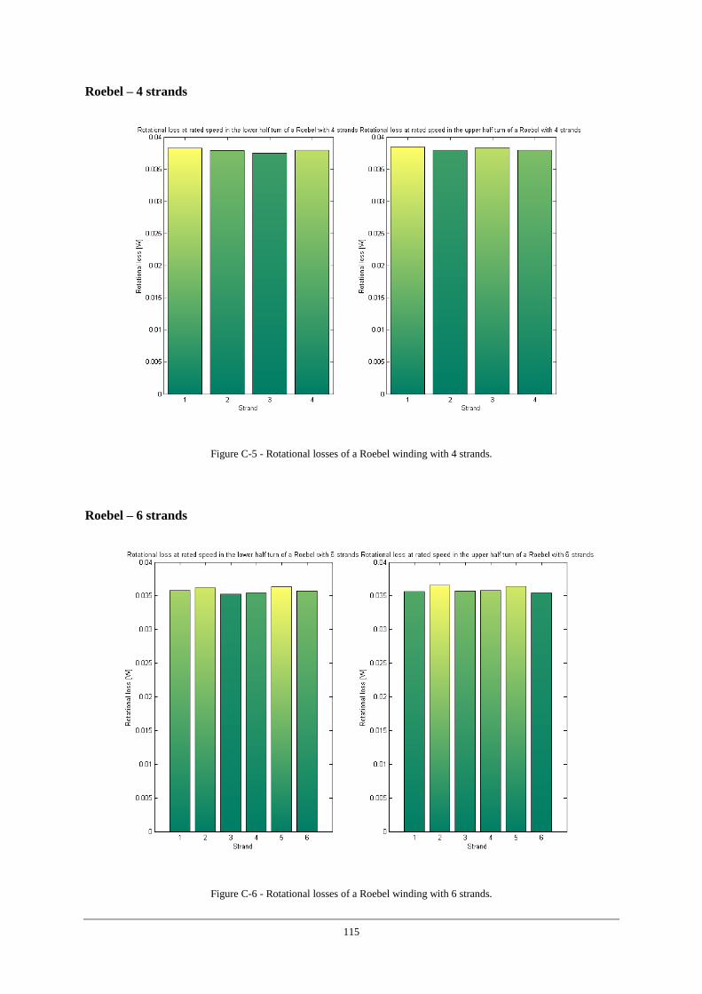
115

Roebel – 4 strands

Figure C-5 - Rotational losses of a Roebel winding with 4 strands.

Roebel – 6 strands

Figure C-6 - Rotational losses of a Roebel winding with 6 strands.

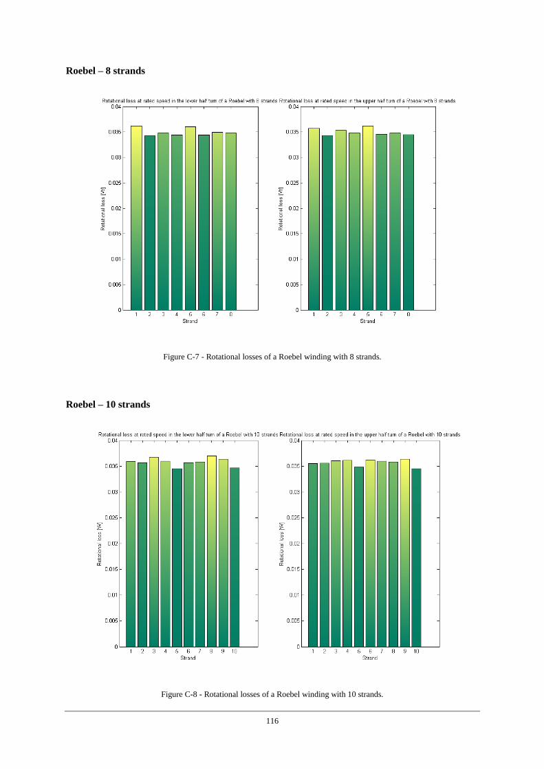
116

Roebel – 8 strands

Figure C-7 - Rotational losses of a Roebel winding with 8 strands.

Roebel – 10 strands

Figure C-8 - Rotational losses of a Roebel winding with 10 strands.

117

Appendix D

Computational effort

118

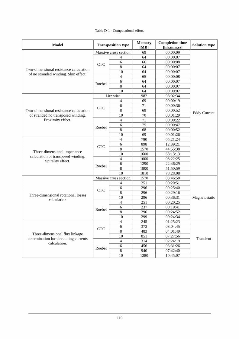
119

Table D-1 - Computational effort.

Model Transposition type Memory

[MB]

Completion time

[hh:mm:ss] Solution type

Two-dimensional resistance calculation

of no stranded winding. Skin effect.

Massive cross section 69 00:00:09

Eddy Current

CTC

4 64 00:00:07

6 66 00:00:08

8 64 00:00:07

10 64 00:00:07

Roebel

4 65 00:00:08

6 64 00:00:07

8 64 00:00:07

10 64 00:00:07

Two-dimensional resistance calculation

of stranded no transposed winding.

Proximity effect.

Litz wire 982 98:02:34

CTC

4 69 00:00:19

6 71 00:00:36

8 69 00:00:52

10 70 00:01:29

Roebel

4 71 00:00:22

6 75 00:00:47

8 68 00:00:52

10 69 00:01:26

Three-dimensional impedance

calculation of transposed winding.

Spirality effect.

CTC

4 790 05:21:24

6 898 12:39:21

8 1570 44:55:38

10 1600 68:13:13

Roebel

4 1000 08:22:25

6 1290 22:46:29

8 1800 51:50:59

10 1810 78:28:08

Three-dimensional rotational losses

calculation

Massive cross section 1570 03:46:58

Magnetostatic

CTC

4 251 00:20:51

6 296 00:25:40

8 296 00:29:16

10 296 00:36:31

Roebel

4 251 00:20:25

6 237 00:19:41

8 296 00:24:52

10 299 00:24:34

Three-dimensional flux linkage

determination for circulating currents

calculation.

CTC

4 245 01:25:23

Transient

6 373 03:04:45

8 483 04:01:49

10 851 07:27:56

Roebel

4 314 02:24:19

6 456 03:31:26

8 940 07:42:40

10 1280 10:45:07

120

121

Appendix E

Dummy stator

122

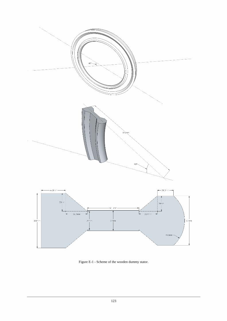
123

Figure E-1 - Scheme of the wooden dummy stator.