Embed Size (px)
Citation preview
Thesis for the Degree of Master of Science in Engineering Physics
Super Yang-Mills Theory usingPure Spinors
Fredrik Eliasson
Fundamental PhysicsChalmers University of Technology
Goteborg, Sweden 2006

Super Yang-Mills Theory using Pure SpinorsFREDRIK ELIASSON
c©FREDRIK ELIASSON, 2006
Fundamental PhysicsChalmers University of TechnologySE-412 96 GoteborgSweden
Chalmers ReproserviceGoteborg, Sweden 2006
Super Yang-Mills Theory using Pure Spinors
Fredrik Eliasson
Department of Fundamental PhysicsChalmers University of Technology
SE-412 96 Goteborg, Sweden
Abstract
The main purpose of this thesis is to show how to formulate super Yang-Millstheory in 10 space-time dimensions using the pure spinor method developedby Berkovits. For comparison we also introduce super Yang-Mills in the ordi-nary component form as well as the usual superspace formulation with con-straints. Furthermore we show how the extra fields in the cohomology of thepure spinor approach can be explained by introducing the antifield formalismof Batalin-Vilkovisky for handling gauge theories.
iii

Acknowledgements
I wish to thank my supervisor Bengt E.W. Nilsson.
iv
Contents
1 Introduction 1
2 SYM and Bianchi identities 3
2.1 Ordinary YM . . . . . . . . . . . . . . . . . . . . . . . . . . . . . 3
2.2 Super Yang-Mills in component form . . . . . . . . . . . . . . . . 4
2.2.1 The abelian case . . . . . . . . . . . . . . . . . . . . . . . . 5
2.2.2 The non-abelian case . . . . . . . . . . . . . . . . . . . . . 8
2.3 Introducing superspace . . . . . . . . . . . . . . . . . . . . . . . 10
2.3.1 Introducing the supermanifold . . . . . . . . . . . . . . . 10
2.3.2 Recalling differential geometry and gauge theory . . . . 12
2.3.3 Back to superspace . . . . . . . . . . . . . . . . . . . . . . 15
2.4 Bianchi identities and their solution . . . . . . . . . . . . . . . . 19
2.4.1 The conventional constraint . . . . . . . . . . . . . . . . . 20
2.4.2 The dynamical constraint . . . . . . . . . . . . . . . . . . 22
2.4.3 Solving the Bianchi identities . . . . . . . . . . . . . . . . 22
2.5 Gauge and SUSY-transformations in superspace . . . . . . . . . 27
3 SYM using pure spinors 33
3.1 The Pure Spinor . . . . . . . . . . . . . . . . . . . . . . . . . . . . 33
3.2 Q and its cohomology . . . . . . . . . . . . . . . . . . . . . . . . 34
v
3.3 More Fields . . . . . . . . . . . . . . . . . . . . . . . . . . . . . . 43
3.3.1 Level zero . . . . . . . . . . . . . . . . . . . . . . . . . . . 43
3.3.2 Level two . . . . . . . . . . . . . . . . . . . . . . . . . . . 45
3.3.3 Level three . . . . . . . . . . . . . . . . . . . . . . . . . . . 46
3.4 Extending to the non-abelian case . . . . . . . . . . . . . . . . . . 46
4 BRST and antifields 49
4.1 Antifields and the master action . . . . . . . . . . . . . . . . . . . 49
4.1.1 Fadeev-Popov quantisation . . . . . . . . . . . . . . . . . 51
4.1.2 BRST-quantisation . . . . . . . . . . . . . . . . . . . . . . 55
4.1.3 BV-quantisation . . . . . . . . . . . . . . . . . . . . . . . . 59
4.2 Antifields for super Yang-Mills . . . . . . . . . . . . . . . . . . . 63
5 Conclusions 67
A Some conventions 69
B Spinors and γ-matrices in D=10 71
B.1 Spinors . . . . . . . . . . . . . . . . . . . . . . . . . . . . . . . . . 71
B.2 Fierzing . . . . . . . . . . . . . . . . . . . . . . . . . . . . . . . . . 74
B.3 Some γ-matrix identities . . . . . . . . . . . . . . . . . . . . . . . 76
C Solving the pure spinor constraint 79
vi
Chapter 1
Introduction
The usual framework for describing the fundamental structure of matter andinteractions in nature is that of quantum field theory (QFT). A specific QFT isgiven by specifying its action, a functional of the different fields of the theory,which can be used to calculate all measurable quantities of interest. The per-haps most interesting property of any action is the symmetries is possesses. Bydemanding that an action should satisfy certain symmetries we can severelylimit the fields it can contain and the shape it can take. The most common ex-ample is that for a QFT to be compatible with the theory of special relativity wehave to demand symmetry under global Lorentz transformation. By studyingthe algebra of the generators of these symmetry transformations we can findexactly what fields can be allowed to appear in the action.
Note that we said global Lorentz transformations. This means that we are con-sidering a continuous family of transformations parametrised by one or moreconstants on space-time. It is then of course natural as a next step to considertransformations with parameters that are functions on space-time. These kindof symmetries are known as gauge symmetries. It turns out that the inter-actions we can observe in nature are described very well by gauge theories— theories that possess gauge symmetries — e.g. quantum electrodynamics,quantum chromodynamics and the standard model. All of these theories areYang-Mills theories — a specific kind of gauge theory.
In the ordinary Standard Model there is a problem related to the Higgs particlesmass — the hierarchy problem — which can be solved by introducing a newrather peculiar symmetry called supersymmetry (SUSY). The simplest modi-fication of the standard model that includes SUSY is the Minimal Supersym-metric Standard Model (MSSM) which also has the added benefit of couplingconstant unification. The introduction of SUSY means enlarging the Poincaregroup by postulating a new symmetry transformation that relates fermionsand bosons. At the moment there are no firm indications that such a symmetryactually exists in nature, but nevertheless it is an interesting subject to study.Aside from the problems mentioned above, the quest to unify gravity with
1
2 CHAPTER 1. INTRODUCTION
quantum mechanics through for instance string theory has led to predictionsof supersymmetry.
In this thesis we will study super Yang-Mills theory (SYM). This is simply thetheory you arrive at when you try to make ordinary Yang-Mills theory super-symmetric. Specifically our aim is to show how SYM can be formulated using arelatively recently discovered method that involves what is called pure spinors.First we will briefly discuss the simplest formulation of SYM — that of simplywriting down the action in therms of the involved fields. This we call the com-ponent formalism. We will then go on to describe the so called super-spaceformulation of SYM and then demonstrate how this is related to the new purespinor formulation. Finally we will introduce some very general tools for thequantization of gauge theories, the Batalin-Vilkovisky formulation (BV), to ex-plain some additional elements that appear in the pure spinor formulation ascompared to the super-space one.
Chapter 2
Super Yang-Mills in D=10from constrained Bianchiidentities
2.1 Ordinary YM
The most convenient way to formulate a Yang-Mills theory is to utilise thelanguage of differential forms. The reason is that the gauge invariance of Yang-Mills theory then can be seen as being due to the nilpotency of the exteriorderivative, d2 = 0, and thus becomes completely transparent.
If we introduce the gauge potential as a 1-form, A = Aµdxµ, and then simplylet the field strength be the 2-form, F = dA, we will immediately have gaugeinvariance under A → A + dΛ, where Λ is an arbitrary 0-form. This is truebecause then we have δF = d(dΛ) = d2Λ = 0.
Expanding the forms in their components one finds that this corresponds di-rectly to the usual formulation of Maxwell’s electromagnetism. That is Fµν =∂µAν − ∂ν Aµ and the transformation Aµ → Aµ + ∂µΛ.
Of course Maxwell’s theory is only a very particular type of Yang-Mills theory,namely the abelian one, but this formalism can also be extended to non-abeliantheories. The exterior derivative then has to be extended to a covariant versionD.
Because F = dA, for the abelian case, it’s obvious that F satisfies the identitydF = 0. This identity is known as the Bianchi identity. In fact as long as ourspacetime has no topological subtleties, saying that F satisfies the Bianchi iden-tity implies that it’s possible to construct F from a gauge potential the way wehave done. In the non-abelian case there is also a Bianchi identity involving
3
4 CHAPTER 2. SYM AND BIANCHI IDENTITIES
the covariant exterior derivative in a similar way. The equivalence betweenconstructing F from a potential A and demanding that it satisfies the Bianchiidentity will be of importance when we try to formulate super Yang-Mills the-ory in superspace.
2.2 Super Yang-Mills in component form
When the Poincare group is extended to the super-Poincare group we needto consider what representations the new group has. Since it consists of bothfermionic and bosonic elements the representation space will have both a fer-mionic and a bosonic sector. Furthermore since the ordinary Poincare groupis a bosonic subgroup both of these sectors should consist of representationsof the Poincare group. A collection of fields living in such a representationof the super-Poincare group is called a supermultiplet. It consists of bosonicand fermionic fields that are mixed when transformed by the supersymmetrygenerators. The supersymmetry transformation maps bosons into fermionsand vice versa. Because of this the degrees of freedom of the bosonic fields inthe multiplet has to equal the degrees of freedom of the fermionic fields.
The simplest example of a supermultiplet is the Wess-Zumino multiplet in fourdimensions. This multiplet contains simply a complex scalar, ϕ, and a Majo-rana spinor, Ψa. The index a in this case takes 4 different values and becauseof the Majorana condition this means that the spinor consists of four real com-ponents if we work in an appropriate basis. The complex scalar on the otherhand can be regarded as being composed of two real components. The numberof components of the fermionic and bosonic fields does obviously not matchas we above claimed they must. The solution is to require that the fields areon-shell. The equation of motion for the scalar is the Klein-Gordon equationand reads p2ϕ = 0. On the mass shell p2 = 0 so ϕ is not restricted in any wayand thus we really have two independent degrees of freedom1. The spinor hasto satisfy the Dirac equation,
(γµ
)a
b pµΨb = 0. Since the Dirac operator, pµγµ,squares to zero on the mass shell2it follows that the dimensionality of its ker-nel is half the dimension of the γ-matrices. We can conclude that the Diracequation halves the number of degrees of freedom in the spinor from four totwo, thus matching the scalar. Note that this matching only occurs when con-sidering on-shell fields. If we wish to work off-shell we must introduce extraauxiliary fields to absorb the difference in number of degrees of freedom.
The SUSY generators are denoted Qa. Their actions on the fields are not par-ticularly complicated but since we do not really need them we will only givethem in a schematic form:
Qaϕ ∼ Ψa (2.1)QaΨb ∼ (γα)ab ∂αϕ
1Chapter ten of [1] has as an elementary introduction to the counting of degrees of freedom.2Since pµγµ pνγν = 1/2pµ pνγµ, γν = pµ pνηµν = p2 = 0.

2.2. SUPER YANG-MILLS IN COMPONENT FORM 5
D Dirac spinor Weyl spinor Maj. spinor Maj.-Weyl spinor Vector
3 4 (2) 2(1) 3 (1)
4 8 (4) 4(2) 4(2) 4 (2)
6 16 (8) 8(4) 6 (4)
10 64 (32) 32 (16) 32 (16) 16(8) 10 (8)
Table 2.1: The number of components of spinors in the dimensions where SYMi possible. The number in parentheses is the degrees of freedom when gaugeinvariance and equations of motion are imposed. The cases that can be used inSYM are boxed. Note that we count real components.
One can check that the the following anticommutation relation is satisfied bythe SUSY generators:
Qa, Qb = 2 (γα)ab Pα (2.2)
where Pα is the ordinary momentum operator that generates translations inspace-time. The standard reference on supersymmetry is [2].
2.2.1 The abelian case
We now wish to construct a supersymmetric version of Yang-Mills theory. Thefields of this theory must live in a supermultiplet and one of the members ofthis multiplet should be a vector corresponding to the gauge field in the ordi-nary theory. In D dimensions a vector has D−2 degrees of freedom. The vectorhas D components and the equation of motion p2 Aµ − pµp · A = 0 reduces topµp · A = 0 on the mass shell which implies that p · A = 0. This can be usedto eliminate one of the components of Aµ in terms of the others, for instanceA0 = pi Ai/p0. At the same time we have the gauge invariance δAµ = pµΛwhich can be used to remove another component of Aµ, for instance A1 bytaking Λ = −A1/p1. Thus the D− 2 degrees of freedom. Note that we will beconsidering only the on-shell case. It is only in certain specific dimension thatit is possible to find a field in a spinorial representation with as many degreesof freedom. One such dimension is D = 10. In this case the vector will have8 degrees of freedom. A Weyl spinor will have 16 complex components. Alsointroducing the Majorana condition (for D = 10 it is possible to impose both theWeyl and the Majorana conditions simultaneously) makes these real. Finallydemanding that the spinor satisfies the Dirac equation gives the desired 8 on-shell degrees of freedom. Super Yang-Mills is also possible for D = 3,4,6. Table2.1 shows the dimensionality of the spinors for these cases. Also see appendixB for more information about the spinors.
The action for our super Yang-Mills theory is
S =Z
d10x[− 1
4Fµν Fµν +
i2χγρ∂ρχ
](2.3)
6 CHAPTER 2. SYM AND BIANCHI IDENTITIES
where F is the ordinary field strength constructed out of the vector in the mul-tiplet as Fµν = ∂µAν − ∂ν Aµ and χa is the Majorana-Weyl spinor with a takingvalues from 1 to 16. Since we are working with Weyl spinors the γ-matricesare really the 16x16 blocks of the ordinary 32x32 γ-matrices in D = 10 in theblock off-diagonal Weyl representation. Once again we refer to appendix B fora further discussion. Varying the action yields the familiar equations of motion:
∂µFµν = 0(γµ
)ab∂µχb = 0(2.4)
Now consider the following supersymmetry transformation on the fields:
(δεA)µ = −(εγµχ
)
(δεχ)a = − i2
Fµν (γµνε)a(2.5)
where ε is a constant Majorana-Weyl spinor parameter. A simple calculationgives the corresponding variation of the action:
δS =Z
d10x[− 1
2Fµν (δεF)µν +
i2(δεχ 6∂χ
)+
i2(χ 6∂δεχ
)]=
=Z
d10x[− Fµν∂
µ(δεA)ν +14
Fµν
(εγµνγρ∂ρχ
)+
14∂ρFµν
(χγργµνε
)]=
=Z
d10x[
Fµν
(εγν∂µχ
)+
14
Fµν
(εγµνγρ∂ρχ
)− 14∂ρFµν
(εγµνγρχ
)]=
=Z
d10x[
Fµν
(εγν∂µχ
)+
14
Fµν
(εγµνγρ∂ρχ
)− 14∂ρ
(Fµν
(εγµνγρχ
))+
+14
Fµν
(εγµνγρ∂ρχ
)]=
=Z
d10x[
Fµν
(εγν∂µχ
)+
12
Fµν
(εγµνγρ∂ρχ
)+ ∂ρ
(· · ·
)]=
=Z
d10x[
Fµν
(εγν∂µχ
)+
12
Fµν
(εγµνρ∂ρχ
)+ Fµν
(εγ[µην]ρ∂ρχ
)+
+ ∂ρ
(· · ·
)]=
=Z
d10x[
Fµν
(εγν∂µχ
)+
12
Fµν
(εγµνρ∂ρχ
)+ Fµν
(εγµ∂νχ
)+ ∂ρ
(· · ·
)]=
=Z
d10x[1
2Fµν
(εγµνρ∂ρχ
)+ ∂ρ
(· · ·
)]=
=Z
d10x[∂ρ
(12
Fµν
(εγµνρχ
))− 12∂ρFµν
(εγµνρχ
)+ ∂ρ
(· · ·
)]=
=Z
d10x∂ρ
(· · ·
)
where we have used that γµγνρ = γµνρ + 2ηµ[νγρ], the symmetry propertiesof the γ-matrices and the spinors, and in the last step the Bianchi identity,∂[µFνρ] = 0. As can be seen the variation consists of a boundary term. Thusthe action is invariant under the SUSY transformation (2.5) if we assume, as isusually done, that the fields goes to zero as x →∞.
2.2. SUPER YANG-MILLS IN COMPONENT FORM 7
To derive the algebra of the generators of our symmetry we will now calculatethe effect of making two successive transformations on a field. Denoting atransformation with parameter εi by δi we get
δ2δ1 Aµ =− δ2(ε1γµχ
)= −(
ε1γµδ2χ)
=i2
Fρσ(ε1γµγρσε2
)=
=i2
Fρσ(ε1γµρσε2
)+ iFρσ
(ε1ηµ[ργσ]ε2
)=
=i2
Fρσ(ε1γµρσε2
)+ iFµσ
(ε1γ
σε2)
If we now use the fact that γµρσ is antisymmetric while γσ is symmetric incombination with the anticommuting property of the εi we get:
[δ1, δ2
]Aµ =− 2iFµσ
(ε1γ
σε2)
(2.6)
Let us now denote the generator of the SUSY transformation by Qa, that isδ1 Aµ = εa
1Qa Aµ. We can then rewrite the commutator of transformations, [δ1, δ2],as an anticommutator of generators, εa
1εb2Qa, Qb. From equation (2.6) we can
thus deduce that
Qa, Qb
Aµ =− 2iFµν
(γν
)ab = −2i∂µAν
(γν
)ab + 2i∂ν Aµ
(γν
)ab =
= ∂µ
(−2iAν
(γν
)ab
)+ 2i
(γν
)ab∂ν Aµ
(2.7)
The first term in this expression is a gauge transformation of A, the second isproportional to the momentum operator, Pµ ∼ ∂µ, in its coordinate realisation.If we instead consider the gauge invariant quantity F we get:
Qa, Qb
Fµν =∂µ
(2i
(γρ
)ab∂ρAν
)− ∂ν
(2i
(γρ
)ab∂ρAµ
)
=2i(γρ
)ab∂ρ
(∂µAν − ∂ν Aµ
)= 2i
(γρ
)ab∂ρFµν
(2.8)
We recognise this as the desired form of the SUSY algebra. Let us now repeatthis calculation but instead acting on the spinor:
δ1δ2χa =− i
2δ1
(Fµν
(γµνε2
)a)
= −i∂µ
(δ1 Aν
)(γµνε2
)a =
=i∂µ
(ε1γνχ
)(γµνε2
)a =i2(ε1γν∂µχ
)[(γµγνε2
)a − (γνγµε2
)a]
=
=− i2εb
1εc2
[(γν
)bd
(γµ
)ae(γν
)ec −
(γν
)bd
(γν
)ae(γµ
)ec
]∂µχd
This leads to[δ1, δ2
]χa =− i
2εb
1εc2
[(γν
)bd
(γµ
)ae(γν
)ec︸ ︷︷ ︸
I
−(γν
)bd
(γν
)ae(γµ
)ec︸ ︷︷ ︸
II
+
+(γν
)cd
(γµ
)ae(γν
)eb︸ ︷︷ ︸
III
− (γν
)cd
(γν
)ae(γµ
)eb︸ ︷︷ ︸
IV
]∂µχd
8 CHAPTER 2. SYM AND BIANCHI IDENTITIES
Terms I and III can be rewritten as:
I + III =(γν
)bd
(γµ
)ae(γν
)ec +
(γν
)cd
(γµ
)ae(γν
)eb =
=3(γµ
)ae(γν
)e(c(γν
)bd) −
(γµ
)ae(γν
)ed(γν
)bc =
=3(γµ
)aeQe
cbd −(γµ
)ae(γν
)ed(γν
)bc
where Q is defined by Qecbd =
(γν
)e(c(γν
)bd). We can utilise the Clifford algebra,(
γµ
)a
b(γν
)b
c +(γν
)a
b(γµ
)b
c = 2ηµνδca, to rewrite terms II and IV as:
II + IV =(γν
)bd
(γν
)ae(γµ
)ec +
(γν
)cd
(γν
)ae(γµ
)eb =
=2(γν
)bdη
µνδac −
(γν
)bd
(γµ
)ae(γν
)ec + 2
(γν
)cdη
µνδab−
− (γν
)cd
(γµ
)ae(γν
)eb =
=2(γµ
)bdδ
ac + 2
(γµ
)cdδ
ab − 3
(γµ
)aeQe
cbd +(γµ
)ae(γν
)ed(γν
)bc
Combining everything we get
[δ1, δ2
]χa =− i
2εb
1εc2
[6(γµ
)aeQe
cbd − 2(γµ
)bdδ
ac − 2
(γµ
)cdδ
ab−
− 2(γµ
)ae(γν
)ed(γν
)bc
]∂µχd =
=− i2εb
1εc2
[6(γµ
)aeQe
cbd − 2(γµ
)bdδ
ac − 2
(γµ
)cdδ
ab−
− 4ηµνδad(γν
)bc + 2
(γν
)ae(γµ
)ed(γν
)bc
]∂µχd =
=− i2εb
1εc2
[6(γµ
)aeQe
cbd − 2(γµ
)bdδ
ac − 2
(γµ
)cdδ
ab−
− 4ηµνδad(γν
)bc + 2
(γν
)ae(γµ
)ed(γν
)bc
]∂µχd
To get to the desired form we will now demand that the spinor χ is on shell,i.e. satisfies the Dirac equation
(γµ
)ab∂µχb = 0, and recall that in D = 10 Qe
abcis identically zero (see appendix B). Only the penultimate term above survivesto give:
Qa, Qb
χc = 2i
(γµ
)ab∂µχc (2.9)
As is noted in the appendix Q vanish also for D = 3,4,6 so we will get thesuper Poincare algebra on-shell in those cases as well. Note however that ,theaction (2.3) was shown to be invariant without using Q. This is an indicationof the fact that this action actually is invariant under the transformations 2.5independently of the dimension or what kind of spinor χ is. We didn’t showthis as our derivation assumed that χ was a Majorana-Weyl spinor in ten di-mensions, but it is possible to do. For further details see [3]. This fact will nolonger be true in the non-abelian case.
2.2.2 The non-abelian case
Everything in section 2.2.1 can be generalised to the non-abelian case. Now thefields, both Aµ and χc, take their values in the gauge Lie algebra. By introduc-ing a basis Ti for the lie algebra we could make this explicit by expanding the
2.2. SUPER YANG-MILLS IN COMPONENT FORM 9
fields like Aµ = AiµTi. However to keeps our formulas clearer we will refrain
from this. Note that in contrast to for instance a fermion in QED here also thespinor is Lie-algebra valued. This is not really strange since it is not a fermionmaking up matter but rather the superpartner to the Lie-algebra valued gaugeboson.
Furthermore, the ordinary derivative ∂µ will have to be replaced by the gaugecovariant derivative ∇µ everywhere it appears. This includes when it is “hid-den” inside the definition of Fµν . The covariant derivative acts in the ordinaryway on Aµ and χc. With our conventions, see appendix A, this is given by
∇µAν = ∂µAν − AµAν
∇µχc = ∂µχc − [Aµ, χc]
The action becomes
S =Z
d10x tr[− 1
4Fµν Fµν +
i2χγρ∇ρχ
](2.10)
where the trace over the algebra has to be introduced to render the action gaugeinvariant. It’s worth pointing out that unlike the abelian case we no longerhave a free theory. The covariant derivative has introduced an interaction be-tween the fields Aµ and χc. We could have included a new parameter in thedefinition of the covariant derivative giving the strength of this interaction.
The equations of motion for the fields are modified to become
(γα
)ab∇αχb = 0
∇αFαβ =i2(γβ
)abχa, χb(2.11)
where we see that the interaction between the fields lead to a current term inthe second equation.
The supersymmetry variations will be exactly the same as before, given inequation (2.5). When verifying the invariance of the new action under thesetransformations one proceeds like in the abelian case. There is however theadded complication that you have to remember to vary also the A-field insidethe covariant derivative. As long as it’s a derivative appearing inside F thiswill, due to cancellations, not give anything new, but because of the covariantderivative in the spinor part of the action a new term appears which meansthat the transformation of the action is proportional to the object Qa
bcd that wedefined earlier. So in the non-abelian case the action is only invariant in thosecases where Q vanish. As we have noted this happens in particular for D = 10.
Working out the algebra one encounters no additional obstacles. On shell it isas expected given by Qa, Qb = 2i
(γα
)ab∇α.
For details on the non-abelian case consult [3] and [4].
10 CHAPTER 2. SYM AND BIANCHI IDENTITIES
2.3 Introducing superspace
As we saw in section 2.1 it is convenient to formulate Yang-Mills theory us-ing the language of differential forms. It is now natural to ask whether ananalogous construction can be made for super Yang-Mills. The answer is “sortof”. Below we will show how we can embed our fields in a super differen-tial form over a supermanifold and then from it construct a field strength andeventually obtain the equations of motion. What we do will however not beto completely mimic the construction of ordinary Yang-Mills theory only re-placing manifold with a supermanifold. We will not gain any complete geo-metric understanding of SYM. The benefit of the superspace formulation to bepresented is rather that the supersymmetry is made completely transparent.In this language supersymmetry transformations will be on an equal footingwith change of coordinates in spacetime. In fact they will be certain coordi-nate transformations on the supermanifold and thus the use of objects thatare inherently coordinate invariant, such as differential forms, will guarantee asupersymmetric theory. The supersymmetry generators will be represented bycertain fermionic derivatives just as the momentum generators are representedby ∂µ. In contrast to the purely bosonic case we will not construct an action toderive the equations of motion. Instead these will arise due to a specific con-straint being imposed on the field strength. Our treatment of super Yang-Millsin superspace is entirely based on [5].
2.3.1 Introducing the supermanifold
A supermanifold, M, is a topological space where each open set can be param-eterised by a set of coordinates ZM = (xµ, θm), where the xµ are commuting realnumbers and the θm are anticommuting real Grassmann numbers. For the casewe consider xµ is a vector with 10 components and θm has 16 components. Thisis of course to match the D = 10 vector and Majorana spinor. We will not bebothered with any global issues and proceed as if the entire manifold could becovered with a single chart. Just as for an ordinary manifold we can introducethe tangent bundle, TM. This is the union of the tangent spaces at all points ofthe manifold. The coordinate basis for the tangent bundle TM consists of thederivatives ∂M = (∂µ, ∂m) = (∂/∂xµ, ∂/∂θm). Note that the derivatives com-mute in the same way as the coordinates. The dual space to TM is the bundleof 1-forms, T∗M or in other words the union of all cotangent spaces. The co-ordinate basis for this bundle is simply the dual basis to the coordinate basisof the tangent bundle. It is usually denoted dZm. It is now of course easy toconstruct higher forms by taking the usual alternating tensor product of oneforms — the ∧-product. One has to be careful though when commuting differ-ent objects and take into account both their form degree and their Grassmannproperties. For instance, if we let |M| = 1 when ZM is anticommuting and|M|= 0 when ZM is commuting we have dZM ∧ dZN =−(−1)|M||N|dZN ∧ dZM.To save some writing we will from now on drop the | · · · | in such expressions.You then have to remember that indices appearing over (−1) are not ordinaryindices and should not be summed over. For forms of higher degree all this
2.3. INTRODUCING SUPERSPACE 11
generalises to(p)ϕ ∧ (q)
ω = (−1)pq+|ω||ϕ| (q)ω ∧ (p)
ϕ
where the form degree is displayed above the forms and |ϕ| = 0 if ϕ is com-muting etc. Note that in the future we will usually not write out the wedgebetween forms. We will denote the space of k-forms by
Vk M and the space ofall forms by
V∗ M. Any k-form can be expanded in terms of the basis elementsdZM1 · · ·dZMk like this:
(k)ω =
1k!
dZMk · · ·dZM1ωM1···Mk
Please note the order of the indices and the fact that we place the componentsafter the forms.
A natural thing to do is to try to define an exterior derivative, d :Vk M →Vk+1 M. Usually it is given by d = dxµ∂µ so a natural generalisation would be
dZM∂M. This is indeed the definition we will adopt though with the addedcomplication that it will act from the right. This is best explained by an exam-ple. On a p-form:
d(p)ω =
1p!
dZMp · · ·dZM1 dZN∂NωM1···Mp
Note that no extra signs appeared since the right action means that d neverhave to commute past the forms dZM, it acts directly on the form componentsstanding on the right. On products of forms the rule is:
d((p)ω ∧ (q)
ϕ)
=(p)ω ∧ d
(q)ϕ + (−1)q d
(p)ω ∧ (q)
ϕ
In the second term d have been commuted past the q-form, thus the extra sign.Also note that d is purely bosonic.
The characteristic property of d is that it satisfies d2 = 0. This is simply encod-ing the fact that partial derivatives commute/anticommute:
d2(p)ω =d2( 1
p!dZMp · · ·dZM1ωM1···Mp
)=
=1p!
d(dZMp · · ·dZM1 dZN∂NωM1···Mp
)=
=1p!
dZMp · · ·dZM1 dZNdZK
︸ ︷︷ ︸(−1)NK+1dZKdZN
∂K∂N︸ ︷︷ ︸(−1)NK∂N∂K
ωM1···Mp =
=0
where the last step follows since the two braced quantities have opposite sym-metries in the N and K indices.
Let us now assume that we have a metric on our manifold. At each pointit is given by an inner product on the tangent space, g(p) : Tp M× Tp M → R.We can express the metric in terms of the coordinate basis, g(VM∂M, WN∂N) =
12 CHAPTER 2. SYM AND BIANCHI IDENTITIES
VMgMNWN , where gMN = g(∂M, ∂N). Now using the metric we can alwaysconstruct another basis for the tangent space that is orthonormal. Let us de-note such a basis by EA = EM
A ∂M. We will assume that the signature of ourmetric is lorentzian. Then the orthonormality is given by, g(EA, EB) = gAB =EM
A gMN ENB =
(ηαβ 0
0 δab
). We will use letters from the beginning of the alphabet,
like A, to denote non-coordinate bases. Letters from the middle of the alphabet,like M, will be reserved for coordinate bases. Note that the orthogonal basis isby no means unique. We can always let the Eα transform as a vector under theLorentz group and the Ea as a Majorana-Weyl spinor. This will not affect theorthonormality. In fact we can make a local Lorentz transformation so that thematrices EM
A depends on where on the manifold we are. We will assume thatEM
A (Z) depends smoothly on Z.
2.3.2 Recalling differential geometry and gauge theory
Before proceeding further with our supermanifold it might be wise to brieflyrecall how you in general do differential geometry and gauge theory. This willhelp us keep our head clear when we try to do the same on the supermanifold.Let us proceed in steps:
1. First let set the stage. We start with a manifold, M. This will always bespacetime. On this manifold we introduce a vector bundle. This we thinkof simply as a union of vector spaces, one for each point of the manifold.A familiar example is the tangent bundle. A trivial vector bundle wouldbe V × M, where V is a vector space and M the manifold, but the inter-esting cases are when the bundle is a so called twisted product between avector space and the manifold. Basically this means that locally the bun-dle is a direct product but when you move to a neighbouring region thevector space above it will have been rotated by some element of a groupG relative to the space over the first region. Of course in reality the groupelement acts on the vector space through some given representation. Thegroup G is called the structure group of the vector bundle and the bundleitself is called a G-bundle. In the case of the tangent bundle this groupwould be the Lorentz group if we decide to use a Minkowski metric.
2. The physical fields will be sections of vector bundles, that is functionsfrom the manifold into the bundle — vector fields if you wish. We willneed to be able to differentiate these sections. To do this there must bea way of comparing vectors that lives in vector spaces at two differentpoints. This is where the connection enters. The connection is really away to do differentiation on sections of bundles. Note that there could bemany different ways to do this for a given vector bundle. Every connec-tion Dv (doing differentiation in the direction of the vector v) can be writ-ten as Dv = vµ∂µ + A(v) where A(v) is an endomorphism on the vectorbundle. As physicists we usually call the endomorphism-valued 1-formA the connection. When working with G-bundles we won’t let A(v) beany old endomorphism. To make the connections “compatible” with the
2.3. INTRODUCING SUPERSPACE 13
structure group we have to require it to belong to the Lie algebra g of G.
3. The physical theories we want should be gauge invariant. This meansthat if we take a particular section of a G-bundle, say s, and for ev-ery point of the manifold act on it with an element of G, that is s → gswhere g : M → G, then the new section gs should describe the samephysics as the original section. What happens to the connections whenwe do gauge transformations? For a given connection D there existsanother one D′ such that D′(gs) = g(Ds). This D′ is the gauge trans-formation of D. In terms of the vector potential A this is expressed asA→ A′ = gAg−1 + gdg−1, when A is Lie-algebra valued this transforma-tion rule makes A′ Lie-algebra valued too. The physics should be invari-ant under gauge transformations of the connection together with gaugetransformations of the fields. Since Ds transform in the same way as s wecall D a covariant derivative.
4. To do gauge invariant physics it’s convenient to have quantities that areinvariant under gauge transformations. One such object that we can con-struct using only the connection is the curvature. It measures how takingcovariant derivatives in different directions fails to commute. It will bea linear function of those two directions, in fact a 2-form. To be morespecific we have
[Dv, Dw
]s = F(v, w)s + D[v,w]s where s is a section of the
vector bundle. F is the curvature 2-form. For a G-bundle it will be Liealgebra-valued just like A. The last term in the expression above is thetorsion term. It appears since it might happen that first moving a smallstep in the direction of v on the manifold and then in the direction of wlands you in a different point than first moving along w and then alongv. Above we implied that the curvature was gauge invariant. This isactually not true. It transform as F → gFg−1. But it’s easy to constructtruly gauge invariant objects from it — you only have to take the trace.Furthermore products of F transform in the same way as F itself.
5. We can regard the connection as a covariant exterior derivative. Let Ebe the bundle we are working on. Then a section s of this bundle willbe an E-valued 0-form. The covariant exterior derivative dD of this willbe an E-valued 1-form. We define it as (dDs)(v) = Dv(s) for a vectorfield v. This then generalises in the natural way to higher forms. Us-ing this language we can define the curvature by d2
Ds = F ∧ s wheres is an E-valued form. Now the torsion term only appears if we ex-pand the left hand side in terms of a basis, say Ea: d2
Ds = dD(Ea Das) =dD(Ea)Das− EadD(Das) = EaEb(Da Dbs + Tc
ab Dcs). Tc = 12 EaEbTc
ba = dDEc
is the torsion 2-form. Starting from a connection on E we can constructa corresponding connection on End(E) and use this to get an exteriorderivative on End(E)-valued forms. This allows us to also do exteriordifferentiation on objects like A and F. We can write the exterior deriva-tives in terms of A as dDs = ds + A ∧ s when s is an E-valued form andas dDB = dB + [A, B] when B is an End(E)-valued form. From the firstone of those you can deduce that F = dA + A∧ A.
6. Since F is an End(E)-valued 2-form we can take the covariant exteriorderivative of it: dDF = dF + [A, F]. By using the formula for F in step 5 it
14 CHAPTER 2. SYM AND BIANCHI IDENTITIES
immediately follows that dDF = 0. This is the Bianchi identity.
That’s all the basics. So let’s move on to the physics. There are two applications:general relativity and gauge theory. We will begin with the first. When doingGR we are working on a base manifold, space-time, that is semi-riemannian.This means that we have a metric — an inner product on the tangent space.Using this metric we can construct an orthonormal basis for the tangent spacea each point. This is exactly what we did for the supermanifold a little earlier.Such a choice of basis for the entire tangent bundle is called a frame and willbe denoted by ea (the orthonormality means that g(ea, eb) = δab). There are ofcourse many different orthonormal bases and the collection of all of them iscalled the frame bundle. Given a particular frame we can do local rotations,ea(x) → e′a(x) = Λb
a(x)eb(x), to get another one. For a minkowskian metric therotations, the matrix Λb
a above, will belong to the Lorentz group. These localLorentz rotations are the gauge transformations we can do on the frame bundlewhose structure group thus is the Lorentz group.
Our fields will be sections of vector bundles associated to the frame bundle.Different representations of the Lorentz group gives different bundles, e.g. vec-tor bundle and spinor bundle. We now have to answer how we are going todecide what connection to use on those bundles. First of all we should recallthat the curvature of space-time is found by solving the Einstein equations. Thecurvature then gives the connection through the equation
R ba = dωb
a + ωca ∧ ωb
c
where we have denoted the connection by ωba . It is a matrix of 1-forms belong-
ing to the Lorentz algebra. To proceed we will have to make an assumption.It is that the connection is torsion free. Remarkably there is only a single con-nection compatible with this assumption for a given metric; the Levi-Civitaconnection. So Einstein’s equations gives curvature, which gives the connec-tion which in turn gives a metric — you only need to solve the differentialequations. The main use of the Levi-Civita connection is that we can formu-late covariant equations of motions for our matter fields by using the covariantderivative constructed with it.
For the special case of flat space the curvature vanishes. You can then showthat there is a choice of orthonormal basis for tangent space so that the connec-tion is zero for all point on the manifold. That is, we can always make a localLorentz transformation on the frame bundle so that the connection potential wtransforms to zero. This does not completely fix the connection. You can stilldo global Lorentz rotations and the connection will remain zero. We can nowmake a suitable choice of coordinates on space-time so that the orthonormalbasis equals the coordinate basis ∂µ for these coordinates. Note that it is onlywhen the torsion is zero that this choice of coordinates is compatible with theglobal vanishing of the connection.
Next up is gauge theory. Since we want both gauge and Lorentz invarianceour matter fields will be sections of the tensor product bundle of a Lorentzbundle and a G-bundle, where G is som Lie group. This means that our con-nection will be of the form dD = d + A +ω where A is g-valued and ω is Lorentz
2.3. INTRODUCING SUPERSPACE 15
algebra-valued as above. The curvature will split in two. One part, R, will bedetermined from ω and measure space-time curvature as before. The otherpart, which we call F, is determined from A and is simply the field strengthof the gauge potential. The curvature part of the connection will be the Levi-Civita connection while A is given by solving the Yang-Mills equation for thefield strength. The Yang-Mills equation follows from the action:
SYM =Z
Mtr(F∧ ∗F)
where ∗ is the usual Hodge star operator. The equation of motion coming fromthis action is dD ∗ F = 0.
For further details of differential geometry and gauge theory [6] is recom-mended.
2.3.3 Back to superspace
We will now apply our knowledge of gauge theory summarised in the lastsection to our supermanifold. Of course the superisation will introduce somedifferences. Commutators are replaced by graded commutators, that is anti-commutator on two fermionic objects, otherwise ordinary commutator, andthings acting from the left are replaced by things acting from the right, specif-ically the exterior derivative and gauge transformations. We have already in-troduced the supermanifold and showed how an orthonormal basis of tangentspace can be locally Lorentz rotated. From now on we will restrict ourselvesto flat superspace. If we had worked in eleven dimensions curved superspacewould have allowed us to derive supergravity, but for now we are only inter-ested in super Yang-Mills. Flat superspace means that the curvature R is zero.We can then choose a basis for our tangent space so that the connection ω iszero everywhere and as above there is a corresponding choice of coordinatesof the supermanifold so that the tangent basis is the coordinate basis. Thesecoordinates will be called ZM.
We will however not use this basis for the tangent bundle but instead use theone spanned by the vectors DA given by:
Dα = ∂α
Da = ∂a − i(γµ
)abθ
b∂µ
(2.12)
Expressed in terms of the coordinate basis this takes the form DA = EMA ∂M
where the matrix EMA is given by
EMA =
(δµα 0
−i(γµθ)a δma
)
We can introduce a corresponding 1-form basis which we denote by EA. It isgiven in terms of the coordinate basis by EA = EA
MdZM where the matrix EAM is
16 CHAPTER 2. SYM AND BIANCHI IDENTITIES
the inverse of EMA . It is easily calculated to be
EAM =
(δαµ 0
i(γαθ)m δam
)
We will now explain why this basis is the preferable one. As we mentionedin the beginning of section 2.3 the purpose of superspace is to realise SUSYtransformations as coordinate transformations. The fields we are interested inare functions of the coordinates of superspace: F = F(Z). When doing the SUSYtransformation they should change like δF = εaQaF where the generator ofthe transformation should satisfy the defining property Qa, Qb = 2
(γµ
)ab Pµ.
Now this should be realised as coordinate transformations. For an arbitrary,small change of coordinates ZM → Z′M = ZM + ξM(Z) we can easily computethe induced change in the field. We should have
F′(Z′) = F(Z)
for corresponding Z and Z′. Taylor expanding gives
F′(Z′) = F(Z′)− ξM(Z′)∂ ′MF(Z′)
were we used that ZM ≈ Z′M − ξM(Z′). If such a change of coordinates reallyshould give a SUSY transformation we would then have to choose ξ so thatεaQa = −ξM∂M, or equivalently that the action of the differential operator Qais εaQaZM =−ξM. Notice that Q generates the coordinate transformation apartfrom a sign, that is δZM = εaQaZM. The sign is the same one that appears whenchanging from active to passive transformations, in fact that’s exactly what weare doing. So what we have to do is to find a differential operator that satisfiesthe defining commutation relation and then minus this operator will give thecoordinate transformations that induces SUSY transformations of the fields.
On the right hand side of the Qa, Qb = 2(γα
)ab Pα the momentum operator
Pα appears. We will work with the definition where Pµ = +i∂µ when actingon the fields. It’s now easy to see that the defining commutation relation isfulfilled by the differential operator Qa = ∂a + i
(γµ
)abθ
b∂µ. Explicitly we have
Qa, Qb = ∂a, ∂b︸ ︷︷ ︸=0
+∂a, i(γµθ
)b∂µ+ i
(γµθ
)a, ∂a−
− (γµθ
)a
(γνθ
)b
[∂µ, ∂ν
]︸ ︷︷ ︸
=0
= i(γµ
)ab∂µ + i
(γµ
)ab∂µ =
= 2i(γµ
)ab∂µ
So to recap, if we do a coordinate transformation ZM → Z′M = ZM − εaQaZwith the Q just defined the induced transformation on the field F(Z)→ F′(Z) =F(Z) + εaQaF(Z) will be precisely a SUSY transformation. However, there is acomplication that we haven’t mentioned yet. The fields we are interested in arenot simply scalar fields on superspace, but rather things like vector fields, 1-forms etc. We expect the spinor and vector field that we had in the componentformulation of super Yang-Mills to sit in the components AM(Z) of a 1-form
2.3. INTRODUCING SUPERSPACE 17
and the change of those components is not so simple under coordinate trans-formations as for the scalar F(Z) above. As an example let us consider a tangentvector to superspace, V = V(Z)M∂M. For an arbitrary coordinate transforma-tion ZM → Z′M = f M(Z) we have ∂M → ∂ ′M = ∂ZN
∂Z′M ∂N . Using the transformedvector basis and the transformed coordinates the expansion of our vector lookslike V = V′M(Z′)∂ ′M. Since the vectorfield itself is independent of both basisand coordinates we should have, for corresponding Z and Z′,
VM(Z)∂M = V′N(Z′)∂ ′N⇔
VM(Z)∂M = V′N(Z′)∂ZM
∂Z′N∂M
⇔
V′N(Z′) = VM(Z)∂Z′N
∂ZM = VM( f−1(Z))∂Z′N
∂ZM
If we now assume that the transformation is small as we did earlier, f M(Z) =ZM + ξM(Z), we can Taylor expand and get
V′N(Z) = VN(Z) +(∂MξN)
VM(Z)︸ ︷︷ ︸rotation term
− ξM∂MVN(Z)︸ ︷︷ ︸transport term
Notice that there are two terms here. One of them, the transport term, is solelydue to the changing coordinates. The other, the rotation term, appears sincethe basis also changes. It is the first of these that would generate the desiredSUSY transformation of the field under coordinate transformations generatedby −Qa defined above. The rotation term however destroys this and meansthat we also get another undesirable term.
It is now that the new basis, introduced in (2.12), comes to the rescue. The Daonly differs by a sign from the SUSY generators Qa and it is exactly this thatmakes them satisfy Da, Qa = 0. Explicitly
Da, Qb = ∂a, ∂b︸ ︷︷ ︸=0
+∂a, i(γµθ
)b∂µ− i
(γµθ
)a, ∂a+
+(γµθ
)a
(γνθ
)b
[∂µ, ∂ν
]︸ ︷︷ ︸
=0
= i(γµ
)ab∂µ − i
(γµ
)ab∂µ = 0
We also trivially have [Dα, Qb] = 0. We now like to see how this basis trans-form when we do the SUSY coordinate transformation. The action of DA onthe coordinates is given by the matrix we introduced earlier: DAZM = EM
A (Z).
18 CHAPTER 2. SYM AND BIANCHI IDENTITIES
Under the transformation this goes to
D′A(ZM − εaQaZM) = EM
A (Z′)⇔
(DA + δDA)(ZM − εaQaZM) = EMA (Z)− εaQaEM
A (Z)⇔
δDAZM − (−1)aAεaDAQaZM = εaQaEMA (Z)
⇔δDAZM − (−1)aAεa[DA, QaZM − εaQa DAZM
︸ ︷︷ ︸=EM
A
= εaQaEMA (Z)
⇔δDAZM = εa[Qa,DAZM ⇔ δDA = εa[Qa,DA = 0
In short our particular basis of tangent vectors does not change when doingcoordinate transformations with Qa. This ensures that the rotation term men-tioned above is eliminated and thus the components of vectors expressed inthis basis really are SUSY-transformed under those changes of coordinates. Allof this works the same way for 1-forms and the dual basis, EA.
We are now ready to introduce gauge theory on superspace. Just as describedin the previous section we should then start with a G-bundle where the gaugegroup G is some Lie group. Note that this will be simply an ordinary group —no superisation. What we really are interested in a connection on this bundle.As mentioned any connection is specified by giving a g-valued 1-form, say A,where g is the Lie algebra of G. A can of course be expanded in the EA-basisand the components will then be SUSY-fields. By adding A to the exteriorderivative we get a covariant exterior derivative. It will be denoted by D andis given by D = d +∧A (note right action) on G-valued sections. We will onlybe dealing with g-valued fields where the action is D = d + [ , A]. Writing outthis in terms of our basis it takes the shape D = EADA = EADA + ∧EA AA forthe first case. The next step is to introduce the field strength 2-form for A:F = 1
2 EAEBFBA. It is easy to derive the equation for F in terms of A followingstep 5 in the previous section (here s is group valued):
s∧ F = D2s = D(ds + s∧ A) = d2s︸︷︷︸=0
+ds∧ A + d(s∧ A) + s∧ A∧ A =
= ds∧ A + s∧ dA− ds∧ A + s∧ A∧ A = s∧ (dA + A∧ A)
(note how F and A acts from the right). Expanding in the orthonormal basisgives:
12
EBEAFAB = d(EC AC) + (−1)ABEBEA AB AA =
= ECEADA AC + d(EC)AC + (−1)ABEBEA AB AA
Here a torsion term appears due to our choice of basis. It is dEC = 12 EAEBTC
BA.So the components of the field strength are
FAB = 2D[A AB + 2(−1)AB A[B AA + TCAB AC (2.13)
2.4. BIANCHI IDENTITIES AND THEIR SOLUTION 19
The components of the torsion are easily calculated using
TC = d(EC) = d(dZMECM) = dZMdEC
M = EDEMD EADAEC
M =
= (−1)A(D+M)EDEAEMD DAEC
M
which gives 12 TC
BA = (−1)B(A+M)EM[ADBEC
M. Plugging in the values of the matri-ces EM
A and ECM given earlier it turns out that all components of the torsion is
zero except forTα
ab = 2i(γα
)ab (2.14)
Using this value for the torsion in equation (2.13) we can write out the differentsuperfield components. They will be of use later:
Fαβ = ∂αAβ − ∂β Aα − [Aα, Aβ] (2.15)Fab = Da Ab + Db Aa −Aa, Ab+ 2i
(γσ
)ab Aσ (2.16)
Fαb = ∂αAb −Db Aα − [Aα, Ab] (2.17)
By expanding D2s in terms of the basis elements we can derive an important re-lation for the covariant derivatives. When s is a group-valued 0-form (bosonic)we have
D2s = D(EADAs) = EAEBDBDAs + d(EA)DAs
which leads toFAB =
[DB,DA+ TC
BADC
Of course this field strength satisfy the Bianchi identity, D F = 0. As in theequation for the field strength we will find that torsion terms appears whenexpanding in the orthonormal basis:
D F = D(12
EAEBFBA) =12
EAEBECDCFBA +14
EAEBECTDCBFDA−
− 14
ECEDTADCEBFBA =
12
EAEBEC(DCFBA + TDCBFDA)
So the Bianchi identity takes the form
D[AFBC + TD[ABF|D|C = 0 (2.18)
This equation will the main topic of the whole next section.
2.4 Bianchi identities and their solution
Writing out the components of the Bianchi identity (2.18), recalling that theonly non-zero torsion component is Tα
ab = 2i(γα
)ab, we get
D[αFβγ] = 0 (2.19)2D[αFβ]c + DcFαβ = 0 (2.20)
DαFbc + 2D(bFc)α + 2iγδbcFδα = 0 (2.21)
D(aFbc) + 2iγδ(abF|δ|c) = 0 (2.22)
20 CHAPTER 2. SYM AND BIANCHI IDENTITIES
Of course these are identities so if F is constructed from A in the prescribedway they will be trivially satisfied. But on the other hand, just as is the case forordinary YM, the Bianchi identities are equivalent to being able to write F interms of A. So instead of working with the potential A we might as well forgetall about it and consider the field strength, satisfying the Bianchi identities, asour fundamental field. This is what we are going to do now. The reason weare doing it this way is that then we do not have to worry about the gaugeinvariance when looking for the physical degrees of freedom. What we wantto do is basically to expand F in a power series in θ and see what physical fieldappear at each level. Those fields will belong to representations of SO(9,1) anddepend only on the x-coordinate.
In ordinary Yang-Mills theory we eliminate the unphysical degrees of free-dom by imposing the Bianchi identity and the equation of motion on the fieldstrength. Normally we would introduce an action to derive the equations ofmotion but here we will proceed in a completely different way. We will byhand impose another set of constraints on the field strength. Then we willshow that those constraints together with the Bianchi identity implies that Fcontains the relevant super Yang-Mills fields and that they satisfy the correctequations of motion. This is very similar to what happens with self-dual fieldstrengths for ordinary Yang-Mills theory in four dimensions. In this case takingthe Hodge dual of a 2-form returns another 2-form so it is possible to considerfields that are self dual: F = ∗F. Since the Bianchi identity is dF = 0 such fieldsautomatically solves d ∗ F = 0 which is the equation of motion.
Of course imposing some ad-hoc constraints with the only motivation that “itworks” feels slightly awkward. Certainly by looking at the field content of theθ-expansion of the different components of F one will find a large number offields that are irrelevant for super Yang-Mills and to end up with this theorythey need to be eliminated by some additional mechanism, only imposing theordinary equation of motion is not enough.
2.4.1 The conventional constraint
Let us start with Fab. Since it has two spinor indices we can expand it in termsof the γ-matrices. Furthermore it is symmetric and both indices have the samechirality so we only need to use γ(1) and γ(5),
Fab = iγαab Fα +
i5!
γα1···α5 Fα1···α5 (2.23)
We can now proceed to expand the field in the first term in powers of θ: Fα(x, θ) =F(0)α (x) + θb F(1)
αb (x) + · · · . The second θ-level can be decomposed in irreps asF(1)αb (x) =
(γα
)b
cF′c(x) + Fαb. Here F is γ-traceless, that is(γα
)a
b Fαb = 0, but theinteresting part is the spinor F′c. After all the theory we are looking for shouldcontain a spinor field. Now let us expand Fαb in the same way
Fαb = Fαb +(γα
)b
c Fc (2.24)
2.4. BIANCHI IDENTITIES AND THEIR SOLUTION 21
where Fαb is γ-traceless. Of course the zeroth θ-level of Fc(x, θ) is a spinor field.This means that we have found two independent spinor fields, so there is atleast one too many.
It is perhaps worth pointing out that both of these fields have a physical di-mension. If we base our calculus of dimensions on the case of four dimensionswhere Fαβ has dimension−2 we can deduce that the 2-form F should be dimen-sionless and thus that [Fab] =−1 and [Fαb] =−3/2 by using that the dimensionof θ and of dθ is 1/2. It then follows that the spinors defined above have di-mension [F′c] = −3/2 and [Fc(x, θ = 0)] = −3/2. Going back to the action incomponent form (2.3) we see that −3/2 is indeed the physical dimension forthe spinor field.
The simplest way to eliminate one of the spinor fields is to put the so calledconventional constraint on our fields
(γβ
)abFab = 0 (2.25)
This is equivalent to Fα = 0. So we get rid of the spinor contained at the firstθ-level of this field, F′c.
If we for a moment go back to Fs definition in terms of A ,see equation (2.16),we notice that the conventional constraint implies the following relation be-tween the components of the connection
Aσ =i
16(γσ
)abDa Ab − i16
(γσ
)ab Aa Ab
Recall that the connection was defined to make a derivative that transform in acovariant way under gauge transformations possible. That is (DAV)→ (DAV)gwhen V → Vg where g is an element of the gauge group in question. It is ob-vious that given a specific connection we can construct a new connection byadding a quantity that is covariant, f → g−1 f g, to the old one. Examples ofquantities that transform in this way are of course the components of the fieldstrength. Let us now assume that AA = (Aα, Aa) is som arbitrary connection.From it we construct a new connection A′
A = (Aα + i/32(γα
)abFab, Aa) using the
just mentioned method. Plugging in the expression for Fab in terms of Aα andAa you can see that the new connection only depends on the components Aaof the old connection: A′
A = (i/16(γα
)abDa Ab − i/16
(γα
)ab Aa Ab, Aa). When we
calculate the field strength for the new connection A′A we find that it automat-
ically satisfies the conventional constraint:
(γσ
)abF′ab = 2(γσ
)abDa A′b − 2
(γσ
)ab A′a A′
b + 2i(γσ
)ab(γα)
ab A′α =
= 2(γσ
)abDa Ab − 2(γσ
)ab Aa Ab + 32iA′σ = 0
The fact that we always can do such a redefinition of the field Aα is why thisconstraint is called conventional.
22 CHAPTER 2. SYM AND BIANCHI IDENTITIES
2.4.2 The dynamical constraint
Imposing only the conventional constraint on the field strength certainly yieldsinteresting results [7, 8], but to get plain and simple super Yang-Mills more isneeded – the dynamical constraint:
(γρ1ρ2ρ3ρ4ρ5
)abFab = 0 (2.26)
This puts Fρaρ2ρ3ρ4ρ5 to zero and together with the conventional constraint elim-inates all of Fab. It is often usefull to instead consider the constraint in the formγ(5)
ab γcd(5)Fcd = 0. The difference is subtle but in this form the self-duality of γ(5)
(as explained in appendix B) can be used to make simplifications in some cal-culations. We will refer to this form of the constraint as the “weak” one.
There are ways to explain this constraint as being due to “integrability on light-like lines”, see [9], but we will not discuss this further in this thesis.
2.4.3 Solving the Bianchi identities
We will now try to find out exactly what our constraints (2.25) and (2.26), to-gether giving
Fab = 0 (2.27)
implies for the fieldstrength components when combined with the Bianchiidentities. Plugging in Fab = 0 in (2.19) to (2.22) yields
D[αFβγ] = 02D[αFβ]c + DcFαβ = 0
2D(bFc)α + 2iγδbcFδα = 0
γδ(abF|δ|c) = 0
(2.28)
The fourth identity
Let us first concentrate on the last one of these. We have already noted that wecan do the decomposition Fαb = Fαb +
(γα
)b
c Fc, which when combined with thelast line of (2.28) gives
(γδ
)(ab F|δ|c) +
(γδ
)(ab
(γ|δ|
)c)
d Fd = 0 (2.29)
In the second term we recognise the combination of γ-matrices denoted Qdabc in
section 2.2.1. We also recall that, as shown in appendix B, Q is identically zeroin D = 10. Thus the last Bianchi identity really says that3 Fδc = 0 or equivalently
Fαb =(γα
)b
c Fc (2.30)
3You can see that this is true by contracting equation (2.29) with(γβ
)ab. You also have to usethat F is γ-traceless.
2.4. BIANCHI IDENTITIES AND THEIR SOLUTION 23
The third identity
Let us now turn to the third equation in (2.28). Recalling Fbα =−Fαb and using(2.30) we get
−2D(b(γ|α|
)c)
d Fd + 2i(γδ
)bcFδα = 0 (2.31)
The symmetry in (bc) means that those two indices can be expanded in terms ofγ(1) and γ(5). Since these are linearly independent the coefficient of each has tobe zero. The coefficients are proportional to the contraction with the respectiveγ-matrix. For γ(1) we get
−2(γβγα
)bdDb Fd + 32iFβα = 0⇔
ηβαCbdDb Fd +(γβα
)bdDb Fd − 16iFβα = 0
Here the middle and last term are antisymmetric in β and α while the first termis symmetric. They thus have to be zero separately. The symmetric part yields
CbdDb Fd = 0 (2.32)
and the antisymmetric part gives
Fαβ = − i16
(γαβ
)abDa Fb (2.33)
We also have to take the contraction of equation (2.31) with γ(5). Because of theorthogonality of the different γ-matrices with respect to the trace only the firstterm in (2.31) survives to give
(γρ1ρ2ρ3ρ4ρ5γα
)bdDb Fd = 0 (2.34)
To proceed any further we will once again have to do an expansion in terms ofγ-matrices, though this time we will have to be slightly careful. If we assumethat the index on the basis form Ea is an anti-Weyl index then obviously theindex on the component Da has to be Weyl. Similarly both indices on Fab shouldbe Weyl, but when doing the expansion in equation (2.30) Fc must have an anti-Weyl index since γ(1) has two indices of the same type. The two indices in Db Fdthus have opposite chirality (but no definite symmetry) so we can expand themas
Db Fd = CbdΛ(0) +(γαβ
)bdΛ(2)
αβ +(γσ1σ2σ3σ4
)bdΛ(4)
σ1σ2σ3σ4
Now we note that equation (2.32) that we just derived from the third Bianchiidentity puts Λ(0) to zero. Similarly equation (2.33) implies that
Fστ = − i16
tr(γστ γαβ)Λ(2)
αβ = 2iΛ(2)στ
Using this expansion in equation (2.34) we find
− i2
tr(γρ1···ρ5γαγβδ)Fβδ − tr(γρ1···ρ5γαγσ1···σ4 )Λ(4)σ1···σ4 = 0

24 CHAPTER 2. SYM AND BIANCHI IDENTITIES
where we for convenience raised and lowered some indices. Utilizing the iden-tity γαγβδ = γαβδ + ηα[βγδ] we see that the first term vanish since it consists oftraces of products of γ-matrices with different number of indices. For the sec-ond term we have the analogous identity γαγσ1···σ4 = γασ1···σ4 + 4ηα[σ1γσ2σ3σ4].Here the first γ has five indices so it survives when traced together with theγρ1···ρ5 giving
16 · 5!δρ1···ρ5ασ1···σ4
Λ(4)σ1···σ4 = 0
By letting ρ1 = α being equal to different values we see that this is the same assaying that Λ(4)
σ1···σ4 = 0.
Finally we can conclude that the third Bianchi identity is equivalent to
Da Fb = − i2(γαβ
)abFαβ (2.35)
The second identity
Using the constraint (2.30) in the second Bianchi identity in (2.28) gives us
DcFαβ + 2(γ[β
)|c|
dDα] Fd = 0 (2.36)
To see what use this equation has let us study the field content of our super-fields. As we have seen the only superfields we have to care about are Fαβ andFc. Fαβ contains at the zeroth θ-level a 2-form field. This is of course the or-dinary x-space field strength. We have no control over the higher θ-levels atthis point. The θ = 0 component of Fc is of course the ordinary spinor in superYang-Mills. The fields at the first θ-level of Fc is equal to the fields at the zerothθ-level of Db Fc since the θ independent part of Db reduces the power of θb byone. Looking at equation (2.35) we can thus conclude that at the first θ-level ofFc we only find the physical 2-form and no new independent fields. We alsosee that all the higher θ-levels of Fc are given by the higher levels of Fαβ . Thefields at the second θ-level of Fc will for instance be those at the first θ-levelof Fαβ . But we can also study the second θ-level of Fc by looking at the zerothθ-level of DaDb Fc.
DaDb Fc =
(2.35)
= − i2(γαβ
)bcDaFαβ
Now we can use (2.36) to rewrite this as
DaDb Fc = i(γαβ
)bc
(γβ
)a
dDα Fd (2.37)
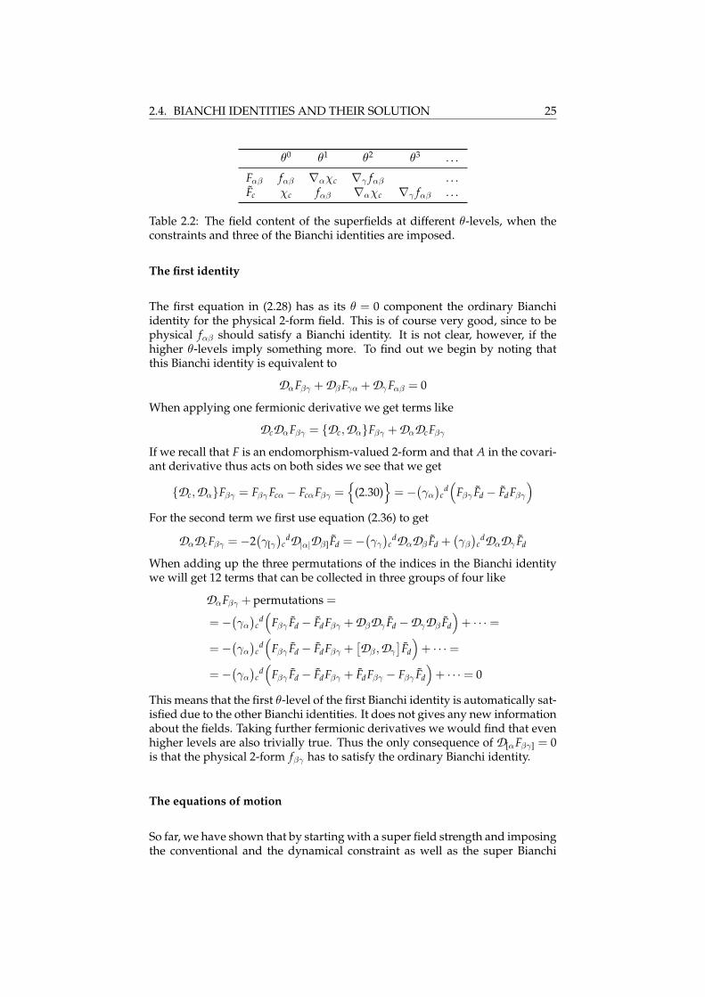
So at the second level of Fc there are no new fields at all, only a derivative ofthe physical spinor. Continuing taking more spinorial derivatives we would,at the higher levels, alternatingly find space-derivatives of the spinor field orthe 2-form field. That is, the only independent fields contained in Fc are the2-form and the spinor of super Yang-Mills. And as noted above there can benothing more at the higher levels of Fαβ either. We will denote the zeroth θlevel of the two superfields by fαβ and χc respectively. The structure of the restof the superfields is then as depicted in table 2.2.
2.4. BIANCHI IDENTITIES AND THEIR SOLUTION 25
θ0 θ1 θ2 θ3 . . .
Fαβ fαβ ∇αχc ∇γ fαβ . . .Fc χc fαβ ∇αχc ∇γ fαβ . . .
Table 2.2: The field content of the superfields at different θ-levels, when theconstraints and three of the Bianchi identities are imposed.
The first identity
The first equation in (2.28) has as its θ = 0 component the ordinary Bianchiidentity for the physical 2-form field. This is of course very good, since to bephysical fαβ should satisfy a Bianchi identity. It is not clear, however, if thehigher θ-levels imply something more. To find out we begin by noting thatthis Bianchi identity is equivalent to
DαFβγ + Dβ Fγα + Dγ Fαβ = 0
When applying one fermionic derivative we get terms like
DcDαFβγ = Dc,DαFβγ + DαDcFβγ
If we recall that F is an endomorphism-valued 2-form and that A in the covari-ant derivative thus acts on both sides we see that we get
Dc,DαFβγ = Fβγ Fcα − FcαFβγ =
(2.30)
= −(γα
)cd(
Fβγ Fd − FdFβγ
)
For the second term we first use equation (2.36) to get
DαDcFβγ = −2(γ[γ
)cdD|α|Dβ] Fd = −(
γγ
)cdDαDβ Fd +
(γβ
)cdDαDγ Fd
When adding up the three permutations of the indices in the Bianchi identitywe will get 12 terms that can be collected in three groups of four like
DαFβγ + permutations =
= −(γα
)cd(
Fβγ Fd − FdFβγ + DβDγ Fd −DγDβ Fd
)+ · · · =
= −(γα
)cd(
Fβγ Fd − FdFβγ +[Dβ ,Dγ
]Fd
)+ · · · =
= −(γα
)cd(
Fβγ Fd − FdFβγ + FdFβγ − Fβγ Fd
)+ · · · = 0
This means that the first θ-level of the first Bianchi identity is automatically sat-isfied due to the other Bianchi identities. It does not gives any new informationabout the fields. Taking further fermionic derivatives we would find that evenhigher levels are also trivially true. Thus the only consequence of D[αFβγ] = 0is that the physical 2-form fβγ has to satisfy the ordinary Bianchi identity.
The equations of motion
So far, we have shown that by starting with a super field strength and imposingthe conventional and the dynamical constraint as well as the super Bianchi
26 CHAPTER 2. SYM AND BIANCHI IDENTITIES
identity, we end up with a theory containing only a 2-form field satisfying thenormal Bianchi identity and a spinor field. These are just the building blocksneeded for super Yang-Mills. The only step left is to write down the equationsof motion. What is remarkable of the superspace formulation of SYM is that wehave already done it! As we will now show the relevant equations of motionhas already been imposed, although not explicitly, by the constraints and thesuper Bianchi identity.
The crucial step is to notice that in the same way as the SUSY generators Qsatisfy their commutation relation, the covariant derivatives satisfy Da,Db=−2i
(γγ
)abDγ . We recognise in the right hand side the Dirac operator which
means that we have
(γα
)a
bDα Fb =i2Da,DbFb = iCbcD(aDb) Fc =
(2.37)
=
= −Cbc(γαβ)
c(b(γβ
)a)
dDα Fd =12
tr(γαβ)︸ ︷︷ ︸=0
(γβ
)a
dDα Fd+
+12(γαβγβ
)︸ ︷︷ ︸
=9γα
adDα Fd =
92(γα
)a
dDα Fd
As the right hand side is proportional to the left hand side (and the constant ofproportionality is not 1) Fc must satisfy the Dirac equation. This of course alsoapplies to its lowest component, the spinor χc:
(γα
)a
c∇αχc = 0 (2.38)
At the second level of Fc we find fαβ . To find out what the Dirac equationmeans for fαβ we apply one fermionic derivative
0 = Dc
((γα
)a
bDα Fb
)=
(γα
)a
b[Dc,Dα
]Fb︸ ︷︷ ︸
I
+(γα
)a
bDαDc Fb︸ ︷︷ ︸II
In term (I) we have to remember that [Dc,Dα]Fb = FbFcα + Fcα Fb (plus in frontof the second term since both Fb and Fcα are fermionic). Recalling that Fcα =−(
γα
)cd Fd we get
I = −(γα
)a
b(γα
)cdFb, Fd
Using equation (2.35) the second term becomes
II = − i2(γα
)a
b(γβγ)
cbDαFβγ = − i2(γαγβγ
)acDαFβγ
2.5. GAUGE AND SUSY-TRANSFORMATIONS IN SUPERSPACE 27
Upon combining the two terms and contracting with(γσ
)ac you get
(γσ
)ac(I + II)
= 0⇔
(γαγσγα
)bd
︸ ︷︷ ︸=−8γσ
Fb, Fd+i2
tr(γσγαγβγ)DαFβγ = 0
⇔−8
(γσ
)bdFb, Fd+i2
tr(γσαγβγ)︸ ︷︷ ︸=2·16δβγ
σα
DαFβγ +i2
tr(ησαγβγ)︸ ︷︷ ︸=0
DαFβγ = 0
⇔
DαFασ =i2(γσ
)abFa, Fb (2.39)
This is the Yang-Mills equation for Fαβ with a current constructed from thespinor Fc. The same equation is also satisfied by the physical fields fαβ and χc.
∇α fασ =i2(γσ
)abχa, χb
This is of course an exact match with the equation given when studying thecomponent formulation.
2.5 Gauge and SUSY-transformations in superspace
We would now like to show that the supersymmetry transformations on thesuperfields generate exactly the same transformations for the component fieldsas those given in chapter 2.2. To this end we will first have to reintroduce thepotential AA and look at its θ-expansion.
Let us begin with recalling that the conventional constraint relates the vectorand spinor part of AA through
Aα =i
16(γα
)ab(Da Ab − Aa Ab)
(2.40)
This mean that we can restrict our attention to Aa since all component fieldswill be contained in it. In particular the zeroth θ-level of Aα appears at the firstlevel of Aa. This field is of course the ordinary gauge potential that gives thefield strength fαβ . We will call it aα.
When working with the field strength we had to consider the Bianchi identities.For the potential we instead have the gauge invariance. It is given by
δAA = DAΛ
28 CHAPTER 2. SYM AND BIANCHI IDENTITIES
where the gauge parameter Λ is a Lie-algebra valued bosonic superfield. Forthe spinor component this gives
δAa = ∂aΛ− i(θγα
)a∂αΛ + [Λ, Aa]
If we expand Aa in powers of θ like Aa = A(0)a + θb A(1)
ab + θb1θb2 A(2)ab1b2
+ · · · and
similarly for Λ, Λ = Λ(0) + θbΛ(1)b + θb1θb2 Λ(2)
b1b2+ · · · , we find that the gauge vari-
ation of the different components becomes
δA(0)a = Λ(1)
a + [Λ(0), A(0)a ]
δA(1)ab = 2Λ(2)
ab − i(γα
)ab∂αΛ(0) + [Λ(1)
b , A(0)a ] + [Λ(0), A(1)
ab ]
δA(2)ab1b2
= 3Λ(3)b1b2a − i
(γα
)ab1∂αΛ(1)
b2+ [Λ(2)
b1b2, A(0)
a ]− [Λ(1)b1
, A(1)ab2
] + [Λ(0), A(2)ab1b2
]
· · ·(2.41)
It is now apparent that by choosing Λ(1) =−A(0)a − [Λ(0), A(0)
a ] we can completelygauge A(0)
a to zero. This is a good thing since A(0)a is a spinor field with the
unphysical dimension [A(0)a ] =−1/2. From now on we will assume that we are
in this specific gauge. The next component is A(1)ab which can be expanded in
terms of a γ(1), a γ(3) and a γ(5)-matrix since the spinor indices have the samechirality and no specific symmetry. Due to the anticommuting property of theθ, Λ(2)
ab will be proportional to only γ(3). We thus see from (2.41) that by choosingΛ(2)
ab properly the γ(3)-part of A(1)ab can be gauged away.
Thus far we have not mentioned the dynamical constraint. It is easy to see thatfor the potential it implies
(γ(5)
)cd
(γ(5))abFab = 0 ⇔ (
γ(5))
cd(γ(5))ab(∂a Ab − i
(θγα
)a∂αAb − Aa Ab) = 0
Note that we here are using the “weaker” form with the extra γ(5)-matrix. Thisis essential for the following calculations to come out right. Each θ-level of theequation has to vanish separately. Since A(0)
a is zero the lowest level (the θ0-level) says that
(γ(5)
)ab A(1)
ba = 0. This will eliminate the γ(5)-part of A(1)ab leaving
only the vector part proportional to γ(1).
From equation (2.41) we see that we still haven’t utilised the terms containingΛ(0) to do gauge transformations with (the term with Λ(1)
a doesn’t enter sinceA(0)
a is zero). If we write what is left of A(1)ab as A(1)
ab =−i(γα
)abaα we see that this
new vector field gauge transform as
δaα = ∂αΛ(0) + [Λ(0), aα]
This is immediately recognised as the gauge transformation of a gauge poten-tial. Furthermore we see from the conventional constraint (2.40) that in ourgauge A(0)
α = aα.
Proceeding with the higher θ-levels of the dynamical constraint and the gaugetransformation we would find that we can choose a gauge such that the spinor
2.5. GAUGE AND SUSY-TRANSFORMATIONS IN SUPERSPACE 29
gauge potential takes the form
Aa = −i(θγα
)aaα − i
36(θγσ1σ2σ3θ
)(γσ1σ2σ3χ
)a+
+124
(γσ1σ2σ3σ4σ5θ
)a
(θγσ1σ2σ3θ
)(∂σ4 aσ5 + aσ5 aσ4
)+ · · ·
(2.42)
It is the coefficient of the third term that requires the “weaker” form of thedynamical constraint. This is because we have to use the duality of the γs toconvert a γ(7) to a γ(3) when calculating it. Doing this we get an ε-tensor that canthen be absorbed in the extra γ(5)-factor due to its self-duality. The expressionabove leads to the following vector part:
Aα = aα −(θγαχ
)+ · · ·
We will now go back to the field strength. We have already indicated the struc-ture of the θ-expansion in table 2.2. Now we would like to have this expansionin its exact form with the correct coefficients etc. To get this you have to usethe equations for the fermionic covariant derivatives acting on Fc derived fromthe Bianchi identities in the last section. When taking θ = 0 in these expressionwe will get equations for the different levels of Fc. Since Da contains Aa we willhave use for the expansion in equation (2.42). The first θ-level is easy to getusing equation (2.35) while the second one requires more involved γ-matrixmanipulations. First we have to put θ = 0 in equation (2.37), taking care not toforget any of the terms on the left hand side:
−i(γβ
)ab∇βχc + 2F(2)
cba = i(γαβ
)bc
(γβ
)a
d∇αχd
where the second level of Fc is given by Fc = . . . + θbθa F(2)cba + . . .. Now the trick
is to expand the a and b indices on the right hand side in terms of the threeγ-matrices
(γσ
)ab,
(γσ1···σ3
)ab and
(γσ1···σ5
)ab. When contracting with the γ(5) we
will get two terms containing a γ(6) and a γ(4) respectively. Using the dualityfrom appendix B we can then rewrite the γ(6) as ε(10)γ
(4). The Levi-Civita ε canthen be gotten rid of using the self-duality of the γ(5) so that we have two termsproportional to
(γσ1···σ5
)ab
(γσ1···σ4
)cd∇σ5χd. Doing the calculation carefully one
luckily finds that these two terms cancel.
Proceeding with the γ(1)-term we get one term with just a δdc and one term with
a(γασ
)cd. The second of these can be rewritten as ηασ − γσγα. Now we see that
when contracting this with ∇αχd the last of those terms will yield the Diracoperator and since χ satisfy the Dirac equation it disappears. The result is thatthe γ(1)-term on the right hand side becomes −i
(γα
)ab∇αχc exactly matching
the γ(1)-term on the left. This means that F(2)cba is equal to the γ(3) part of the right
side. This is not surprising since the contractions with the θs means that a andb are antisymmetric. Explicitly we have
F(2)cba =
5i64
(γασ1σ2
)ab
(γσ1σ2
)cd∇αχd +
i32
(γσ1σ2σ3
)ab
(γασ1σ2σ3
)cd∇αχd
Here we can make a simplification by using the Dirac equation in the sameway as when calculating the γ(1)-term. When γα∇αχ = 0 one can show that
30 CHAPTER 2. SYM AND BIANCHI IDENTITIES
the relation γασ1σ2σ3∇αχ = 3γ[σ2σ3∇σ1]χ is true. This means that the two termsin F(2)
cba combine to one. The full expression for Fc to second order is now givenby
Fc = χc − i2(θγαβ
)c fαβ − i
8(θγσ1σ2σ3θ
)(γσ2σ3∇σ1χ
)c + · · · (2.43)
Having the exact form of Fc up to the second level allows us to calculate Fαβ
to the first level using equation (2.33). For the zeroth level we of course onlyget fαβ while the first level will have a contribution from both the zeroth andsecond level of Fc. From the zeroth level when the θ-part of Da acts on χb aswell as from the anticommutator between χb and A(1)
ac and from the secondlevel due to the ∂a in Da. Specifically these contributions are
Fαβ = · · · − i16
(γαβ
)ab[− i
4(γσ1σ1σ3θ
)a
(γσ2σ3∇σ1χ
)b−
− i(θγσ
)a∂σχb −χb,−i
(θγσ
)aaσ
]+ · · · =
= · · ·+ 164
(θγσ1σ2σ3γαβγσ2σ3∇σ1χ
)− 116
(θγσγαβ∇σχ
)+ · · ·
Rewriting the products of the γ-matrices while utilizing that χc satisfies theDirac equation like above we find that
Fαβ = fαβ − 2(θγ[β∇α]χ
)+ · · · (2.44)
We are now able to consider the supersymmetry transformations. As was ex-plained these are given by the operator Qa. Acting with εaQa on a field wouldgive the SUSY transformation with parameter εa of the field. By looking atthe different θ-levels you can then deduce the transformation properties of thecomponent field. Let us do this first for Fc given in (2.43):
δε Fc =(εQ
)Fc =
(εa∂a + i
(εγαθ
)∂α
)Fc =
= − i2(εγαβ
)c fαβ + i
(εγαθ
)∂αχc − i
4(εγσ1σ2σ3θ
)(γσ2σ3∇σ1χ
)c + · · ·
From this we immediately get that δεχc = − i2 (εγαβ)c fαβ which is exactly the
same transformation as the one defined in equation (2.5). To get the variationof fαβ we could remove the θ and project with a γ(2)-matrix but it is simpler toinstead consider the variation of Fαβ . This gives
δεFαβ = −2(εγ[β∇α]χ
)+ · · ·
We don’t actually need to go further than this first term because it directlyimplies that δε fαβ = −2
(εγ[β∇α]χ
)which is the desired transformation from
equation (2.5). The same transformation would have appeared if we had pro-ceeded with the next θ-level of δε Fc above, but only after slightly harder work.
If we had wished we could have applied the SUSY transformation directly tothe expansions of the gauge fields AA that we derived earlier. The problemwith this though is that it does yield the SUSY transformation of the component
2.5. GAUGE AND SUSY-TRANSFORMATIONS IN SUPERSPACE 31
fields only up to a gauge transformation. To get the same result as above weshould combine a SUSY transformation of AA with a gauge transformation ofAA. This is of course messier than working directly with the gauge covariantfield strengths.

32 CHAPTER 2. SYM AND BIANCHI IDENTITIES
Chapter 3
Super Yang-Mills in D=10using pure spinors
In this chapter we will show how to formulate super Yang-Mills in yet anotherway. Here the equations of motion and gauge variations will arise as a con-sequence of demanding that the physical fields belong to the cohomology ofa certain operator, denoted Q. This operator will be constructed using a cer-tain kind of spinors called pure spinors that we will define shortly. The purespinor approach to SYM was introduced by Berkovits [10, 11, 12]. The originalpurpose was to covariantly quantise the Green-Schwarz superstring, but it isalso applicable to our case. Besides giving us another way to formulate SYMwe will also see that there is something more to this approach – we will findadditional fields.
3.1 The Pure Spinor
To do super Yang-Mills the Berkovits way we have to work with the so calledpure spinor. A pure spinor, λc, is in D = 10 a Weyl spinor satisfying the condi-tion (
λγσλ)
= 0 (3.1)
For this to make sense λc has to be a bosonic parameter rather than fermionicsince otherwise the pure spinor constraint would be trivially true.
Note that because the constraint is completely covariant this defines, in a sense,a representation of the Lorentz group – making a Lorentz transformation of apure spinor will yield another pure spinor — the pure spinors does howevernot form a module. It can be shown that the pure spinor constraint reduces thenumber of independent components to 11. To show this it is simplest to breakthe manifest Lorentz symmetry and choose another basis for the γ-matrices.
33

34 CHAPTER 3. SYM USING PURE SPINORS
We will however not have any need for this result so this calculation has beenrelegated to appendix C.
The pure spinor was first introduced by Cartan in a slightly different form andfor other purposes [13]. There are earlier attempts to utilize pure spinors whentrying to formulate a theory of SYM that closes off-shell [14].
3.2 Q and its cohomology
Let us define the operator Q by
Q = λa Da = λa(∂a − i (γαθ)a∂α) (3.2)
where λ is a pure spinor. This Q should not be confused with the SUSY gen-erator Qa. It is easy to show that Q is nilpotent when acting on an arbitraryfield:
Q2Ψ =(λa∂a − i(λγαθ)∂α
)(λb∂b − i(λγβθ)∂β
)Ψ =
= λaλb∂a∂bΨ︸ ︷︷ ︸I
− i(λγβλ
)∂βΨ︸ ︷︷ ︸
II
+ iλa(λγβθ)∂β∂aΨ︸ ︷︷ ︸
III
− iλb(λγαθ)∂α∂bΨ︸ ︷︷ ︸
IV
−
− i(λγαθ
)(λγβθ
)∂α∂βΨ︸ ︷︷ ︸
V
= 0
Here I is zero because the product of the two pure spinors is symmetric whilethe two derivatives are anticommuting, II is zero because of the pure spinorconstraint, III and IV cancel each other and V vanish because of the oppositesymmetry in the α and β indices on the γ-matrices compared to the derivatives.
One of the things that are interesting to calculate for a nilpotent operator is itscohomology. For a nilpotent operator acting on a vector space, Q : Λ → Λ, thecohomology is the quotient vector space
H(Q) =Ker(Q)Im(Q)
or in words the Q-closed elements that are not Q-exact. In our case the spaceΛ is the space of functions of the variables xα, θa and λa. More specifically wewill restrict ourselves to functions that can be expanded in a power series inpositive powers of θa and λa. Because of the antisymmetry the highest powerof θ is 16. A general function in the space Λ can thus be expanded as
A(x, θ, λ) = A(0,0) + · · · +θb1 · · · θb16 A(0,16)b1···b16
+
+ λa1 A(1,0)a1
+ · · · +λa1θb1 · · · θb16 A(1,16)a1b1···b16
+
+ λa1λa2 A(2,0)a1a2
+ · · · +λa1λa2θb1 · · · θb16 A(2,16)a1a2b1···b16
+
...
3.2. Q AND ITS COHOMOLOGY 35
Notice that this power expansion introduces a natural bigrading of the vectorspace: Λ = ⊕i, jΛ(i, j), where Λ(i, j) is the subspace of functions with θ-power jand λ-power i. The operator Q has one term that increases the θ-level by oneand one term that decreases it. We will denote the two terms with Q+ and Q−
respectively. Both of those adds one to the λ-level. Thus the total Q acts on thesubspaces like Q : Λ(i, j) → Λ(i+1, j−1) ⊕Λ(i+1, j+1).
Since Q does not mix the different λ-levels we can consider the cohomologyon each subspace of a specific λ-power separately. If we define the subspaceΛ(i) =
L16j=1 Λ(i, j) and let Q(i) be the restriction of Q to Λ(i) the cohomology
for a given power i of λ is given by H(i)(Q) = H(Q(i)) = Ker(Q(i))/Im(Qi−1).The complete cohomology can be reconstructed from the subcohomologies:H(Q) =
Li H(i)(Q).
We will now start our calculation of the cohomology of Q by considering onlythe first λ-level, H(1)(Q). In this case the space of fields is given by functions onthe form λa Aa(x, θ) where Aa can be expanded like
Aa(x, θ) = a(0)a (x) + θb1 a(1)
ab1(x) + · · ·+ θb1 · · · θb16 a(16)
ab1···b16(x)
If a particular field configuration is to belong to the cohomology it must sat-isfy the equation 0 = Qλa Aa = λcDcλa Aa = λcλaDc Aa where the last equalityfollows since Dc contains no derivatives with respect to λa. Now the two in-dices on the λs can be expanded in γ-matrices. Since the pure spinors arecommuting the only possible terms are the one proportional to γ(1) and the oneproportional to γ(5). However due to the pure spinor constraint the first one ofthese is killed. We thus have
λcλa =1
16 · 5!(γσ1···σ5
)ca(λγσ1···σ5λ)
and the equation for the Q-closed elements is equivalent to(γ(5)
)abDa Ab = 0.
This equation will be referred to as the equation of motion. We must of coursenot forget that in the cohomology we have to identify fields only differing bysomething Q-exact. We can interpret this as the following gauge-invariance:λaδAa = QΩ = λaDaΩ. Here Ω ∈ Λ(0) and can be expanded like
Ω(x, θ) = ω(0)(x) + θb1ω(1)b1
(x) + · · ·+ θb1 · · · θb16ω(16)b1···b16
(x)
To proceed we will look at what our two equations means level by level in θ.The lowest level of the gauge invariance says that
δa(0)a = ω(1)
a
It is apparent that by choosing ω(1)a appropriately we can always gauge a(0)
a tozero and the superfields in the cohomology will thus not contain this compo-nent. Moving on to the next level we have
λaθbδa(1)ab = λaθb
(2ω(2)
ab − i(γσ
)ab∂σω(0)
)
Now it’s time to do some γ-expansion. There is no symmetry between a and bin a(1)
ba so the expansion will contains term proportional to γ(1), γ(3) and γ(5). ω(2)ab
36 CHAPTER 3. SYM USING PURE SPINORS
on the other hand is completely antisymmetric so here the only term is the onewith γ(3). Now we see that we can use ω(2)
ab to gauge away the γ(3)-part of a(1)ba . If
we now turn to the zeroth level of the equation of motion we see that this saysthat (
γ(5))aba(1)ba = 0
This obviously tells us that also the γ(5)-term is zero. We conclude that a(1)ab must
take the form a(1)ab =−i
(γα
)abaα where the constant is chosen with the benefit of
hindsight. Furthermore the term containing ω(0) in the gauge-variance meansthat δaα = ∂αω(0). This is certainly starting to look familiar, but there is more tocome!
Moving up to the second θ-level the gauge invariance is
λaθb1θb2δa(2)ab1b2
= λaθb1θb2
(3ω(3)
ab1b2− i
(γσ
)ab1∂σω(1)
b2
)(3.3)
We will have to expand a(2)ab1b2
in irreps. Of course due to the antisymmetry the
b indices must be sitting on a γ(3), a(2)ab1b2
=(γσ1σ2σ3
)b1b2 kaσ1σ2σ3 , leaving only the
expansion of the 3-form- spinor kaσ1σ2σ3 . Earlier we have used that a vector-spinor can be expanded like Vaα = Vaα +
(γα
)absb, where the tilde denotes
γ-tracelessness and sb is a cospinor. This type of expansion can be extendedto other tensor-spinors. A given n-form-spinor can be expanded in one γ-tracelessness part and terms with γ(1) up to γ(n)-matrices. These matrices willbe multiplied with appropriate γ-traceless tensor-spinors with enough vectorindices to give a total of n in each term. To keep the correct symmetry allvector indices must be antisymmetrised. As an example consider a 2-form-spinor Vαβa. To begin with we can do the expansion Vαβa = Vαβa +
(γ[αTβ]
)a +(
γαβ S)
a, where Tbβ is a vector-cospinor and Sb is a spinor. Using the decom-
position of a vector-cospinor into a traceless part and a spinor part that can beabsorbed into the Sb term we get Vαβa = Vαβa +
(γ[αTβ]
)a +
(γαβ S
)a. It is easy to
convince yourself that if you try to include terms with higher γ-matrices thanγ(2) they can always be rewritten as a sum of terms like the ones we alreadyhave. The case of a 3-form-spinor is now straightforward:
kaσ1σ2σ3 = kaσ1σ2σ3 +(γ[σ1 s1
σ2σ3]
)a +
(γ[σ1σ2 s2
σ3]
)a +
(γσ1σ2σ3 s
)a
Here k is a 3-form-spinor, s1 is a 2-form-cospinor, s2 is a vector-spinor and s isa cospinor. The first three all have vanishing γ-trace.
Returning to the gauge variation we have ω(3)ab1b2
on the right hand side withall indices antisymmetric. Of course we can still do the same expansion as fora(2)
ab1b2in the b indices
ω(3)ab1b2
=(γσ1σ2σ3
)b1b2
[maσ1σ2σ3 +
(γ[σ1 r1
σ2σ3]
)a +
(γ[σ1σ2 r2
σ3]
)a +
(γσ1σ2σ3 r
)a
]
Since each term belongs to a separate irrep the additional antisymmetry of thea index has to be present in each one of the terms by itself. To investigatethis we project with
(γτ1τ2τ3
)ab1 . When doing this we get several products of
γ-matrices, one for each term, that have to be calculated. For doing this the

3.2. Q AND ITS COHOMOLOGY 37
Mathematica package GAMMA [15] is recommended. This will lead to thefollowing identities for the different terms:
(γσ1σ2σ3
)b1b2 maσ1σ2σ3 =
12(γτ1τ2τ3
)b1amb2τ1τ2τ3
(γσ1σ2σ3
)b1b2
(γ[σ1 r1
σ2σ3])
a = −(γτ1τ2τ3
)b1a
(γ[τ1 r1
τ2τ3
)b2
(γσ1σ2σ3
)b1b2
(γ[σ1σ2 r2
σ3]
)a =
12(γτ1τ2τ3
)b1a
(γ[τ1τ2 r2
τ3]
)b2
(γσ1σ2σ3
)b1b2
(γσ1σ2σ3 r
)a =
12(γτ1τ2τ3
)b1a
(γτ1τ2τ3 r
)b2
Of these only the second has the desired antisymmetry. Thus the traceless 2-form-spinor is the only field in the expansion that isn’t necessarily zero: ω(3)
ab1b2=(
γσ1σ2σ3)
b1b2
(γ[σ1 r1
σ1σ2]
)a.
After this long exercise in γ-matrix expansions we can finally return to thegauge variation. Comparing the expansions on both sides it is obviously al-ways possible to choose r1
aσ1σ2so that the corresponding term in a(2)
ab1b2is gauged
away. I.e. s1aσ1σ2
= 0. To get information on the other irreps in a(2)ab1b2
we will nowlook at the equation of motion at the first θ-level. It says that
(γ(5))a1a2θb1
(2a(2)
a2a1b1− i
(γα
)a1b1∂αa(0)
a2
)= 0 (3.4)
Of course as we already have pointed out a(0)a2 can be gauged to zero so we can
disregard the second term. When contracting the γ(5) with the expansion ofa(2)
a2a1b1we get the following different terms
(γσ1σ2σ3γτ1τ2τ3τ4τ5 kσ1σ2σ3
)b2
= −480(γ[τ1τ2 kτ3τ4τ5])
b2(γσ1σ2σ3γτ1τ2τ3τ4τ5γσ1σ2 s2
σ3
)b2
= 80(γ[τ1τ2τ3τ4 s2
τ5])
b2(γσ1σ2σ3γτ1τ2τ3τ4τ5γσ1σ2σ3 s
)b2
= 0
that we have calculated using GAMMA. These equations means that due tothe Q-closedness kaσ1σ2σ3 and s2
aσ both have to be zero. They cannot cancel eachother since they belong to different irreps. All that remains at the second θ-level of Aa is thus a(2)
ab1b2= − i
36
(γσ1σ2σ3
)b1b2
(γσ1σ2σ3χ
)a where we have rescaled
the cospinor in a convenient way.
The reader will by now have realised that the field Aa belonging to the Q-cohomology contains the same component fields as the gauge field Aa we gotfrom the constrained superspace in the last chapter. To investigate this furtherwe would now like to move on to the higher θ-levels, but the expansion offields with more and more spinor indices would become prohibitively cum-bersome. There would be too many terms living in different irreps making usloose track of what we’re doing. Fortunately we can simplify the expansionprocess by using the computer program LiE [16]. The equations we are deal-ing with typically have the following spinor index structure Aa1···am Ba1···am = 0(there might be uncontracted spinor indices that are not written out). The ob-ject B lives in the space Sm and A lives in Cm where S and C are the vectorspaces
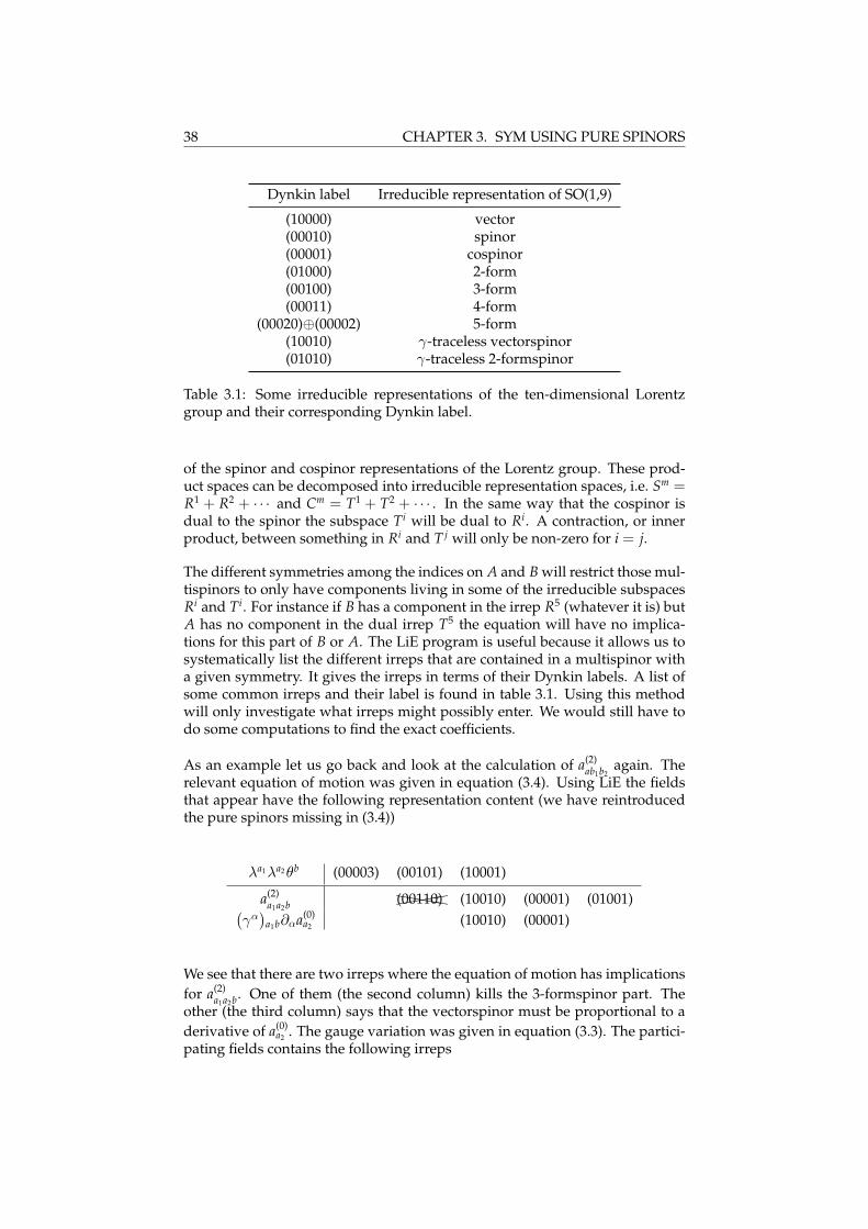
38 CHAPTER 3. SYM USING PURE SPINORS
Dynkin label Irreducible representation of SO(1,9)
(10000) vector(00010) spinor(00001) cospinor(01000) 2-form(00100) 3-form(00011) 4-form
(00020)⊕(00002) 5-form(10010) γ-traceless vectorspinor(01010) γ-traceless 2-formspinor
Table 3.1: Some irreducible representations of the ten-dimensional Lorentzgroup and their corresponding Dynkin label.
of the spinor and cospinor representations of the Lorentz group. These prod-uct spaces can be decomposed into irreducible representation spaces, i.e. Sm =R1 + R2 + · · · and Cm = T1 + T2 + · · · . In the same way that the cospinor isdual to the spinor the subspace Ti will be dual to Ri. A contraction, or innerproduct, between something in Ri and T j will only be non-zero for i = j.
The different symmetries among the indices on A and B will restrict those mul-tispinors to only have components living in some of the irreducible subspacesRi and Ti. For instance if B has a component in the irrep R5 (whatever it is) butA has no component in the dual irrep T5 the equation will have no implica-tions for this part of B or A. The LiE program is useful because it allows us tosystematically list the different irreps that are contained in a multispinor witha given symmetry. It gives the irreps in terms of their Dynkin labels. A list ofsome common irreps and their label is found in table 3.1. Using this methodwill only investigate what irreps might possibly enter. We would still have todo some computations to find the exact coefficients.
As an example let us go back and look at the calculation of a(2)ab1b2
again. Therelevant equation of motion was given in equation (3.4). Using LiE the fieldsthat appear have the following representation content (we have reintroducedthe pure spinors missing in (3.4))
λa1λa2θb (00003) (00101) (10001)
a(2)a1a2b ((((hhhh(00110) (10010) (00001) (01001)(
γα)
a1b∂αa(0)a2 (10010) (00001)
We see that there are two irreps where the equation of motion has implicationsfor a(2)
a1a2b. One of them (the second column) kills the 3-formspinor part. Theother (the third column) says that the vectorspinor must be proportional to aderivative of a(0)
a2 . The gauge variation was given in equation (3.3). The partici-pating fields contains the following irreps

3.2. Q AND ITS COHOMOLOGY 39
λaθb1θb2 (00010) (00101) (01010) (10001)
a(2)ab1b2
(00001) (01001) (10010)ω(3)
ab1b2(01001)(
γσ)
ab1∂σω(1)b2
(00001) (10010)
Here we have only included the reps in a(2)ab1b2
that are still left after the equationof motion have been applied. There is one match in the third column whichtells us that the traceless 2-formspinor can be gauged away. Furthermore wesee from the last column that the vectorspinor, which above was shown to beproportional to a derivative of a(0)
a , can be gauge transformed with a derivativeof ω(1)
a . This is not surprising since we already know that a(0)a is put to zero by
choosing ω(1)a properly. Thus choosing ω(1)
a so that a(0)a vanish will also remove
the vectorspinor in a(2)ab1b2
. The only remaining part of a(2)ab1b2
is then the cospinor.
In the gauge variation the term with ω(1)a also has a cospinor part but since ω(1)
has already been used to put a(0)a to zero there is no freedom left to do anything
more and so we still have all degrees of freedom left in the cospinor. The resultwe have reached is the same as what we got earlier by doing the full explicitexpansion.
Now that we have introduced this more schematic method for expansion ofmultispinors we are able to proceed to the second θ-level of the equation ofmotion and the third θ-level of the gauge variation without the complicationof doing an explicit expansion. First the gauge variation:
λaθb1θb2θb3
(δa(3)
ab1b2b3− 4ω(4)
ab1b2b3+ i
(γα
)ab1∂αω(2)
b2b3
)= 0
LiE tells us that the relevant irreps are
λaθb1θb2θb3 (00011) (01000) (01011) (10100) (02000) (10020)
a(3)ab1b2b3
(00011) (01000) (01011) (10100) (02000) (10002)
ω(4)ab1b2b3b4
(02000) (10002)(γα
)ab1∂αω(2)
b2b3(00011) (01000) (10100)
The two rightmost irreps contained in a(3)ab1b2b3
in this table can be gauge to zero.
Three of the four others gaugetransform with a derivative on ω(2)b2b3 . Since ω(2)b2b3
was used to gauge parts of a(1)ab to zero there is no freedom left in this field to do
further transformations. On to the equation of motion:
λa1λa2θb1θb2
(3a(3)
a2a1b1b2− i
(γα
)a1b1∂αa(1)
a2b2
)= 0
Now the table of irreps looks like this
λa1 λa2 θb1θb2
(00011) (00102) (01000) (01011) (10002) (10100)
a(3)a2a2b1b2
(((hhh(00011) (01000) (((hhh(01011) (((hhh(10100)(γα
)a1b1
∂αa(1)a2b2
(01000) (00000) (20000)
40 CHAPTER 3. SYM USING PURE SPINORS
This immediately yields that three of the four remaining parts of a(3)ab1b2b3
mustbe zero. The only nontrivial part is thus a 2-form which should be given bysome expression involving ∂αa(1)
a1b2. To deduce the exact expression we must
find a way to combine γ-matrices and the 2-form into an expression with fourspinor indices with the same symmetry as a(3)
ab1b2b3. This is actually easy. The
last two b indices are antisymmetric so they can be put on a γ(3)-matrix. Nowplace the other two indices on a γ(5)-matrix and then contract the vector in-dices on the γ(3) with those on the γ(5). This leaves two antisymmetric vectorindices on the γ(5) that can be contracted with the 2-form. The ansatz is thusa(3)
ab1b2b3=
(γσ1···σ5
)a[b1
(γσ1σ2σ3
)b2b3] pσ4σ5 . Here we had to put in the explicit an-
tisymmetrisation since we don’t write out the θs. You could be worried thatthis might lead to the identical vanishing of our expression. Compare for in-stance to
(γσ
)a(b
(γσ
)cd) which we know is zero. However, as can be verified by
contracting for instance the b1 and b2 index with a γ(3), this is not the case.
Of course the ansatz we have written down is not the only possibility with thedesired symmetry. Specifically there are two other ways to write such terms:(γσ1
)a[b1
(γσ1σ2σ3
)b2b3] pσ2σ3 and
(γσ1σ2σ3
)a[b1
(γσ1σ2
σ4)
b1b2] pσ3σ4 . However since weknow a priori from the LiE-expansion that there should be only one 2-form ina(3) all the different ways to write this out must be related to each other. Theexact relations are possible to work out by Fierz expanding in the differentpairs of indices. Doing this you find that the different terms satisfy
(γσ1···σ5
)a[b1
(γσ1σ2σ3
)b2b3] pσ4σ5 = −6
(γσ1
)a[b1
(γσ2σ3
)b2b3] pσ3σ4 =
= −3(γσ1σ2σ3
)a[b1
(γσ1σ2
σ4)
b2b3] pσ3σ4
It is thus OK for us to decide to work with only one of the forms.
If we use, as was shown earlier, that a(1)ab = −i
(γα
)abaα the 2-form part of the
equation of motion says that(λγσ1···σ5λ
)(θγσ1σ2σ3θ
)pσ4σ5 − 2
(λγσ1···σ5θ
)(λγσ1σ2σ3θ
)pσ4σ5−
− (λγαθ
)(λγβθ
)∂αaβ = 0
To get something out of this equation we have to rewrite each term in a canoni-cal way. We do this by a Fierz expansion of the indices the two λs in the secondand third terms are contracted with. Since the pair of λs can only sit on a γ(5)
due to their pureness we get
(λγσ1···σ5λ
)(θγσ1σ2σ3θ
)(pσ4σ5 −
288016 · 5!
pσ4σ5 −40
16 · 5!∂σ4 aσ5
)= 0
To arrive at this result the duality between γ(7) and γ(3) as well as the self-duality of γ(5) had to be used (see appendix B). We see that the 2-form weare looking for is really given by the field strength constructed from the vec-tor potential: pαβ = 1
14 ∂[αaβ]. This still matches the spinor potential from thesuperspace construction, though only if we assume an abelian gauge group.
There might not appear to be any benefits of continuing the calculation of thecohomology to higher orders, but there is! Already at the next level some in-teresting things will start to happen so we push on. We proceed exactly in the
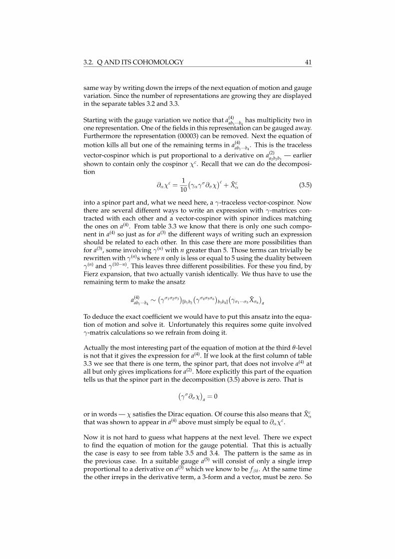
3.2. Q AND ITS COHOMOLOGY 41
same way by writing down the irreps of the next equation of motion and gaugevariation. Since the number of representations are growing they are displayedin the separate tables 3.2 and 3.3.
Starting with the gauge variation we notice that a(4)ab1···b4
has multiplicity two inone representation. One of the fields in this representation can be gauged away.Furthermore the representation (00003) can be removed. Next the equation ofmotion kills all but one of the remaining terms in a(4)
ab1···b4. This is the traceless
vector-cospinor which is put proportional to a derivative on a(2)a2b2b3
— earliershown to contain only the cospinor χc. Recall that we can do the decomposi-tion
∂αχc =110
(γαγσ∂σχ
)c + Xcα (3.5)
into a spinor part and, what we need here, a γ-traceless vector-cospinor. Nowthere are several different ways to write an expression with γ-matrices con-tracted with each other and a vector-cospinor with spinor indices matchingthe ones on a(4). From table 3.3 we know that there is only one such compo-nent in a(4) so just as for a(3) the different ways of writing such an expressionshould be related to each other. In this case there are more possibilities thanfor a(3), some involving γ(n) with n greater than 5. Those terms can trivially berewritten with γ(n)s where n only is less or equal to 5 using the duality betweenγ(n) and γ(10−n). This leaves three different possibilities. For these you find, byFierz expansion, that two actually vanish identically. We thus have to use theremaining term to make the ansatz
a(4)ab1···b4
∼ (γσ1σ2σ3
)[b1b2
(γσ4σ5σ6
)b3b4]
(γσ1···σ5 Xσ6
)a
To deduce the exact coefficient we would have to put this ansatz into the equa-tion of motion and solve it. Unfortunately this requires some quite involvedγ-matrix calculations so we refrain from doing it.
Actually the most interesting part of the equation of motion at the third θ-levelis not that it gives the expression for a(4). If we look at the first column of table3.3 we see that there is one term, the spinor part, that does not involve a(4) atall but only gives implications for a(2). More explicitly this part of the equationtells us that the spinor part in the decomposition (3.5) above is zero. That is
(γσ∂σχ
)a = 0
or in words — χ satisfies the Dirac equation. Of course this also means that Xcα
that was shown to appear in a(4) above must simply be equal to ∂αχc.
Now it is not hard to guess what happens at the next level. There we expectto find the equation of motion for the gauge potential. That this is actuallythe case is easy to see from table 3.5 and 3.4. The pattern is the same as inthe previous case. In a suitable gauge a(5) will consist of only a single irrepproportional to a derivative on a(3) which we know to be fβδ . At the same timethe other irreps in the derivative term, a 3-form and a vector, must be zero. So
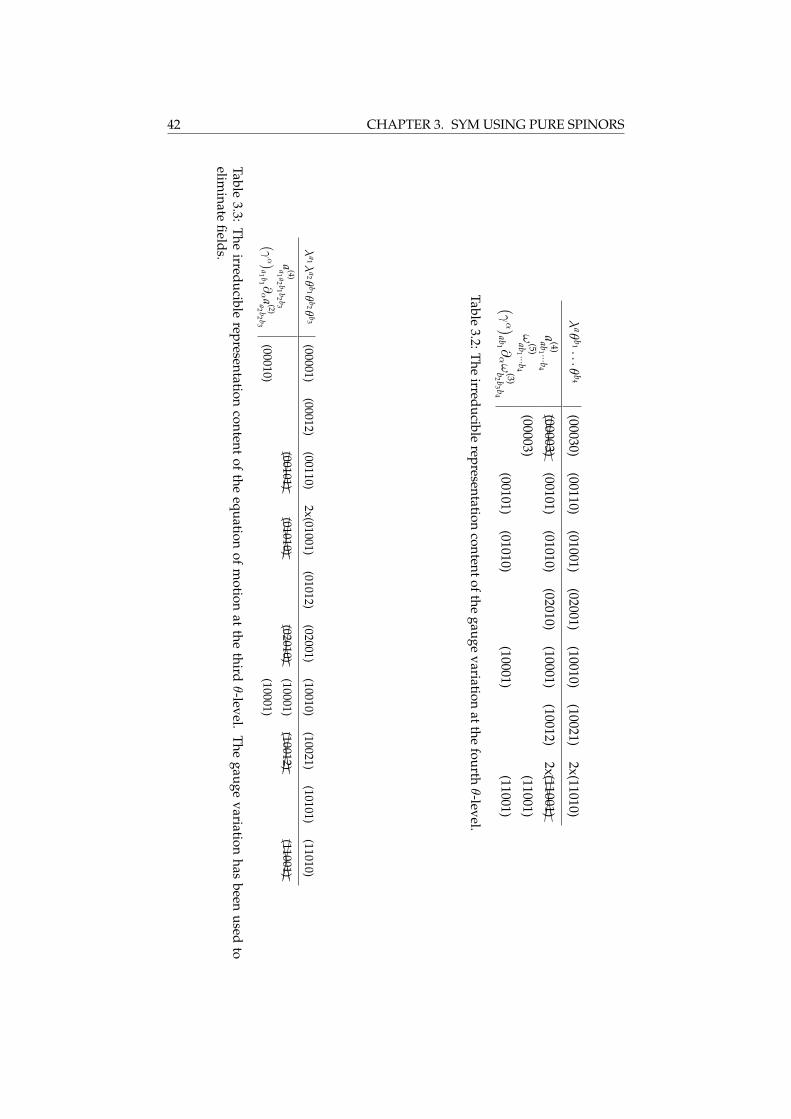
42 CHAPTER 3. SYM USING PURE SPINORS
λaθ
b1···θ
b4
(00030)(00110)
(01001)(02001)
(10010)(10021)
2x(11010)
a(4)ab
1 ···b4
((
( (h
hhh
(00003)(00101)
(01010)(02010)
(10001)(10012)
2x((
( (h
hhh
(11001)
ω(5)ab
1 ···b4
(00003)(11001)
(γα )
ab1 ∂
αω
(3)b
2 b3 b
4(00101)
(01010)(10001)
(11001)
Table3.2:The
irreduciblerepresentation
contentofthegauge
variationatthe
fourthθ-level.
λa1λ
a2θb1θ
b2θb3
(00001)(00012)
(00110)2x(01001)
(01012)(02001)
(10010)(10021)
(10101)(11010)
a(4)a1 a2 b1 b2 b3
((
( (h
hhh
(00101)(
(( (
hh
hh(01010)
((
( (h
hhh
(02010)(10001)
((
( (h
hhh
(10012)(
(( (
hh
hh(11001)
(γα )
a1 b1 ∂α a
(2)a2 b2 b3
(00010)(10001)
Table3.3:
Theirreducible
representationcontent
ofthe
equationof
motion
atthe
thirdθ-level.
Thegauge
variationhas
beenused
toelim
inatefields.
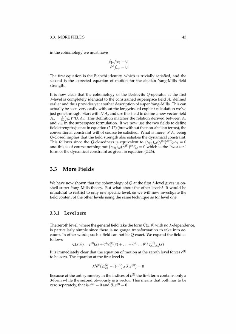
3.3. MORE FIELDS 43
in the cohomology we must have
∂[α fβδ] = 0∂α fαβ = 0
The first equation is the Bianchi identity, which is trivially satisfied, and thesecond is the expected equation of motion for the abelian Yang-Mills fieldstrength.
It is now clear that the cohomology of the Berkovits Q-operator at the firstλ-level is completely identical to the constrained superspace field Aa definedearlier and thus provides yet another description of super Yang-Mills. This canactually be seen very easily without the longwinded explicit calculation we’vejust gone through. Start with λa Aa and use this field to define a new vector fieldAα = i
16
(γα
)abDa Ab. This definition matches the relation derived between Aa
and Aα in the superspace formulation. If we now use the two fields to definefield strengths just as in equation (2.17) (but without the non-abelian terms), theconventional constraint will of course be satisfied. What is more, λa Aa beingQ-closed implies that the field strength also satisfies the dynamical constraint.This follows since the Q-closedness is equivalent to
(γ(5)
)cd
(γ(5)
)abDa Ab = 0
and this is of course nothing but(γ(5)
)cd
(γ(5)
)abFab = 0 which is the “weaker”
form of the dynamical constraint as given in equation (2.26).
3.3 More Fields
We have now shown that the cohomology of Q at the first λ-level gives us on-shell super Yang-Mills theory. But what about the other levels? It would beunnatural to restrict to only one specific level, so we will now investigate thefield content of the other levels using the same technique as for level one.
3.3.1 Level zero
The zeroth level, where the general field take the form C(x, θ) with no λ-dependence,is particularly simple since there is no gauge transformation to take into ac-count. In other words, such a field can not be Q-exact. We expand the field asfollows
C(x, θ) = c(0)(x) + θa1 c(1)a1
(x) + . . . + θa1 . . . θa16 c(16)a1...a16
(x)
It is immediately clear that the equation of motion at the zeroth level forces c(1)
to be zero. The equation at the first level is
λaθb(2c(2)ab − i
(γα
)ab∂αc(0)) = 0
Because of the antisymmetry in the indices of c(2) the first term contains only a3-form while the second obviously is a vector. This means that both has to bezero separately, that is c(2) = 0 and ∂αc(0) = 0.

44 CHAPTER 3. SYM USING PURE SPINORS
λaθ
b1···θb5
(00020)(00031)
2x(01020)(01100)
(10011)(11000)
(11011)(12000)
(20020)(20100)
a(5)ab1 ...b5
(00002)(00013)
2x((
( (h
hhh
(01002)(01100)
(10011)(11000)
(11011)(12000)
(20002)(
(( (
hh
hh(20100)
ω(6)ab1 ···b5
(01002)(20100)
(γα )
ab1 ∂α ω
(4)b2 ···b5
(00002)(01002)
(01100)(10011)
(11000)(12000)
(20002)
Table3.4:The
irreduciblerepresentation
contentofthegauge
variationatthe
fifthθ-level.
λa1
λ a2θ b1···θ b4
(00002)(00020)
(00031)(00100)
(00111)(01002)
(01020)(01100)
(02002)(10000)
2x(10011)(10022)
(11000)2x(11011)
(12000)(20020)
a (5)a1 a2 b1 ···b4
((
hh
(00002)(
(h
h(00013)
((
hh
(01002)(
(h
h(01100)
((
hh
(10011)(11000)
((
hh
(11011)(
(h
h(12000)
((
hh
(20002)
(γα )a1 b1
∂α
a (3)a2 b2 b3 b4
(00100)(10000)
(11000)
Table3.5:The
irreduciblerepresentation
contentoftheequation
ofmotion
atthefourth
θ-level.Thegauge
variationhas
beentaken
intoaccount.
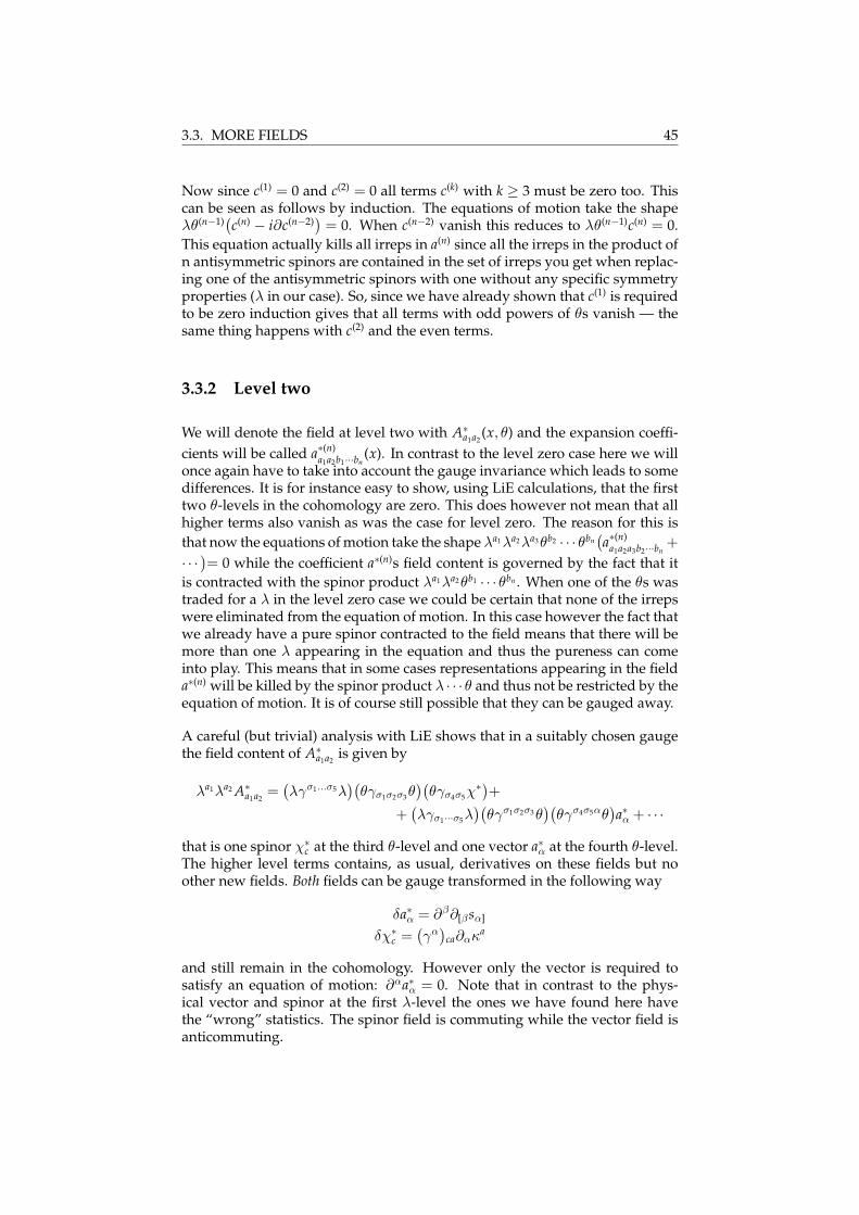
3.3. MORE FIELDS 45
Now since c(1) = 0 and c(2) = 0 all terms c(k) with k ≥ 3 must be zero too. Thiscan be seen as follows by induction. The equations of motion take the shapeλθ(n−1)
(c(n) − i∂c(n−2)
)= 0. When c(n−2) vanish this reduces to λθ(n−1)c(n) = 0.
This equation actually kills all irreps in a(n) since all the irreps in the product ofn antisymmetric spinors are contained in the set of irreps you get when replac-ing one of the antisymmetric spinors with one without any specific symmetryproperties (λ in our case). So, since we have already shown that c(1) is requiredto be zero induction gives that all terms with odd powers of θs vanish — thesame thing happens with c(2) and the even terms.
3.3.2 Level two
We will denote the field at level two with A∗a1a2
(x, θ) and the expansion coeffi-cients will be called a∗(n)
a1a2b1···bn(x). In contrast to the level zero case here we will
once again have to take into account the gauge invariance which leads to somedifferences. It is for instance easy to show, using LiE calculations, that the firsttwo θ-levels in the cohomology are zero. This does however not mean that allhigher terms also vanish as was the case for level zero. The reason for this isthat now the equations of motion take the shape λa1λa2λa3θb2 · · · θbn
(a∗(n)
a1a2a3b2···bn+
· · ·)= 0 while the coefficient a∗(n)s field content is governed by the fact that itis contracted with the spinor product λa1λa2θb1 · · · θbn . When one of the θs wastraded for a λ in the level zero case we could be certain that none of the irrepswere eliminated from the equation of motion. In this case however the fact thatwe already have a pure spinor contracted to the field means that there will bemore than one λ appearing in the equation and thus the pureness can comeinto play. This means that in some cases representations appearing in the fielda∗(n) will be killed by the spinor product λ · · · θ and thus not be restricted by theequation of motion. It is of course still possible that they can be gauged away.
A careful (but trivial) analysis with LiE shows that in a suitably chosen gaugethe field content of A∗
a1a2is given by
λa1λa2 A∗a1a2
=(λγσ1...σ5λ
)(θγσ1σ2σ3θ
)(θγσ4σ5χ
∗)++
(λγσ1···σ5λ
)(θγσ1σ2σ3θ
)(θγσ4σ5αθ
)a∗α + · · ·
that is one spinor χ∗c at the third θ-level and one vector a∗α at the fourth θ-level.The higher level terms contains, as usual, derivatives on these fields but noother new fields. Both fields can be gauge transformed in the following way
δa∗α = ∂β∂[βsα]
δχ∗c =(γα
)ca∂ακa
and still remain in the cohomology. However only the vector is required tosatisfy an equation of motion: ∂αa∗α = 0. Note that in contrast to the phys-ical vector and spinor at the first λ-level the ones we have found here havethe “wrong” statistics. The spinor field is commuting while the vector field isanticommuting.
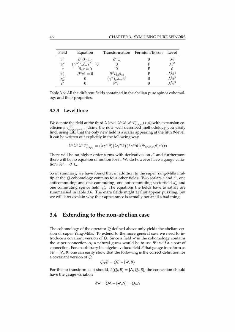
46 CHAPTER 3. SYM USING PURE SPINORS
Field Equation Transformation Fermion/Boson Level
aα ∂β∂[βaα] ∂αω B λθχa
(γα
)a
b∂αχb = 0 0 F λθ2
c ∂αc = 0 0 F 0a∗α ∂αa∗α = 0 ∂β∂[βsα] F λ2θ4
χ∗a 0(γα
)ab∂ακb B λ2θ3
c∗ 0 ∂αtα B λ3θ5
Table 3.6: All the different fields contained in the abelian pure spinor cohomol-ogy and their properties.
3.3.3 Level three
We denote the field at the third λ-level λa1λa2λa3 C∗a1a2a3(x, θ) with expansion co-
efficients c∗(n)a1a2a3b1···bn
. Using the now well described methodology you easilyfind, using LiE, that the only new field is a scalar appearing at the fifth θ-level.It can be written out explicitly in the following way
λa1λa2λa3 C∗a1a2a3=
(λγσ1θ
)(λγσ2θ
)(λγσ3θ
)(θγσ1σ2σ3θ
)c∗(x)
There will be no higher order terms with derivatives on c∗ and furthermorethere will be no equation of motion for it. We do however have a gauge varia-tion: δc∗ = ∂αtα.
So in summary, we have found that in addition to the super Yang-Mills mul-tiplet the Q-cohomology contains four other fields: Two scalars c and c∗, oneanticommuting and one commuting, one anticommuting vectorfield a∗α andone commuting spinor field χ∗c . The equations the fields have to satisfy aresummarised in table 3.6. The extra fields might at first appear puzzling, butwe will later explain why their appearance is actually not at all a bad thing.
3.4 Extending to the non-abelian case
The cohomology of the operator Q defined above only yields the abelian ver-sion of super Yang-Mills. To extend to the more general case we need to in-troduce a covariant version of Q. Since a field Ψ in the cohomology containsthe super-connection Aa a natural guess would be to use Ψ itself a a sort ofconnection. For an arbitrary Lie-algebra valued field B that gauge transform asδB = [Λ, B] one can easily show that the following is the correct definition fora covariant version of Q
QΨB = QB− [Ψ, BFor this to transform as it should, δ(QΨB) = [Λ, QΨB], the connection shouldhave the gauge variation
δΨ = QΛ− [Ψ,Λ] = QΨΛ
3.4. EXTENDING TO THE NON-ABELIAN CASE 47
The equation of motion for Ψ should similarly be defined as
QΨΨ = QΨ−ΨΨ = 0
Note that now all the fields should take values in the Lie algebra correspondingto the non-abelian gauge group.
Is the new QΨ still nilpotent? The answer is yes, but only on shell. Note thatfor a Ψ′ on the form Ψ′ = Ψ + δΨ = Ψ + QΨΛ we have
QΨ′Ψ′ = QΨ′ −Ψ′Ψ′ = QΨ + Q(QΨΛ)− (Ψ + QΨΛ)(Ψ + QΨΛ) ≈≈ QΨ− Q[Ψ,Λ]−ΨΨ−Ψ, QΛ+ Ψ, [Ψ,Λ] == QΨΨ− [QΨ,Λ]− [Λ,ΨΨ] = QΨΨ + [Λ, QΨΨ]
to the first order in Λ. This means that if Ψ belongs to the kernel of the covari-ant Q so does a Ψ′ in the form above trivially. It is thus meaningful to considerthe cohomology as before. A careful analysis shows that the independent fieldcontent doesn’t change. However the equations of motions and the gauge vari-ations are modified and turns out to give
∇α f αβ =i2(γβ
)abχa, χbδaα =∇αω(γα
)a
c∇αχc = 0δχc = [ω,χc]
...
We see that the physical (in the sense that we now what they are, not that theyare gauge invariant) fields aα and χc now satisfy the equations of non-abeliansuper Yang-Mills. So the modification we did to Q appears to be the correctone.

48 CHAPTER 3. SYM USING PURE SPINORS
Chapter 4
BRST and antifields
4.1 Antifields and the master action
So far we have been dealing with the classical super Yang-Mills theory, but wedo of course know that for any theory to be applicable to the real world it hasto be quantised. However, gauge theories are generically problematic in thisregard due to the fact that infinitely many field configurations (those relatedby gauge transformations) describe exactly the same physical situation. Thismeans that in the partition function
Z =Z
DϕeiS[ϕ]
you will be summing over the same integrand infinitely many times whichleads to a divergent result. For the time being we will be working with somegeneric gauge theory with the all the fields collectively denoted ϕ. It is fre-quently stated that this resulting infinity means that simply doing the naivepath integral is wrong for gauge theories. This is however not really the prob-lem. You have to remember that what you really would like to do is to computematrix elements of some operator O[ϕ] and the formula for doing this is of thefollowing form
〈α|O |β〉 =R
DϕO[ϕ]eiS[ϕ]R
DϕeiS[ϕ]
If O is a gauge invariant operator, as it should be to be observable, the samedivergence will be present in both the nominator and denominator of this ex-pression and thus cancel each other. So the matrix elements could possiblystill be finite and meaningful. The real problem with the gauge invariance hasrather to do with the perturbation expansion. A general action takes the formS = S0 + Si where S0 is the part of the action that is quadratic in the fieldsand governs their dynamics. The term Si is the interaction part. When in-serted in the path integral the part due to the interaction terms can be Tay-lor expanded (assuming a small coupling) meaning that we in reality only
49
50 CHAPTER 4. BRST AND ANTIFIELDS
have to be able to calculate correlation functions for the free theory whichis given by the quadratic part of the action. Now note that by introducingdelta functions and doing partial integrations we can always write this part asS0 =
R Rdxdyϕ(x)K(x, y)ϕ(y) for some K. The gauge invariance means that the
complete action satisfiesZ
dxδS
δϕ(x)δϕ(x) = 0
where δϕ(x) is the transformation of the field ϕ(x). We will write this as δϕ(x) =RdyR[ϕ](x, y)α(y) with α(y) as the parameter of the gauge transformation.
Note that this form of writing the variation can accommodate derivatives onα since they by partial integration can be included in R. Now if we take a func-tional derivative with respect to ϕ(y) on the expression for the variation of theaction above we find
Zdx
δ2Sδϕ(y)δϕ(x)
δϕ(x) +Z Z
dxdzδS
δϕ(x)δR[ϕ](x, z)
δϕ(y)α(z) = 0
If we recall that δS/δϕ(x) actually gives the equation of motion and thus iszero for fields that are on shell we see that if we evaluate the above equationfor such a field — let’s call it ϕ0 — we get
Zdx
δ2Sδϕ(y)δϕ(x)
∣∣∣ϕ=ϕ0
δϕ0(x) = 0
Unless the action contains terms linear in the field, identically equal to zerowill be a solution to the equations of motion and for this particular choice ofϕ0 the second derivative on S in the integrand above reduces to the quadraticpart of the action, exactly what we denoted K earlier. So this small calculationthus shows that K has zero modes
ZdxK(y, x)V(x) = 0
where the vector with zero eigenvalue, V(x), is given byR
dzR[0](x, z)α(z). Thepoint of all this is that it means that K lacks an inverse. This can easily be seenas follows. Recall that the definition of the inverse is
ZdzK−1(x, z)K(z, y) = δ(x− y)
If we let the left hand side act on the (nonzero) vector V(y) we getZ
dzdyK−1(x, z) K(z, y)V(y)︸ ︷︷ ︸=0
= 0
The right hand side would of course yield V(x) thus implying that V = 0 whichis a contradiction. So in this case K−1 must be nonexistent. As is well knownthe inverse of K is the propagator and it is essential when computing the cor-relation functions. Thus we see that the existence of the gauge invarianceprohibits us from doing perturbation theory using the ordinary Feynman dia-grams. There is however a small problem with the argument above. We could

4.1. ANTIFIELDS AND THE MASTER ACTION 51
equally well restrict α(x) to be a constant. We would then be dealing with aglobal symmetry but still find that the quadratic part of the action has zeromodes. But we know from experience that global symmetries does not stopus from finding propagators so obviously there has to be something more to itthan we have said so far. The answer lies in the fact that the amount of zeromodes is far greater in the case of a local symmetry. There is one for everyfunction α(x) whereas in the global case there is only one for every constant α.Note that even if an operator is zero on a subspace it still has an inverse whenrestricted to the rest of the space. In the case of the global symmetry the spaceof zero modes is so small that it does not matter in the path integral — it hasmeasure zero so to speak. Whereas for the gauge case there are actually fielddegrees of freedom with no propagator.
4.1.1 Fadeev-Popov quantisation
It is apparent that we can’t do perturbation theory with an action that is gaugeinvariant and to circumvent this problem we have to come up with an equiva-lent action, in the sense that it yields the same physics, but without the gaugeinvariance. The standard way to do this is by the Fadeev-Popov procedure.This procedure is discussed, more or less clear, in almost any book on quan-tum field theory. One of the better is [17], even though the treatment therediffers somewhat from ours.
The essence of this method is that we really should only need to sum onceover each physically distinct field configuration. When doing the naive pathintegral we integrate over the whole space of field configurations illustrated infigure 4.1. Starting from a given field the gauge slice or gauge orbit this fieldbelongs to is constructed by performing all possible gauge transformations onthe field. All fields in the slice describe the same physics. By choosing a suitablefunction F(ϕ) of the fields and demanding that F(ϕ) = 0 we can pick out onefield from every slice. F(ϕ) = 0 is thus a gauge fixing condition. Now it shouldbe possible to rewrite the path integral so that the integration over the fieldϕ(x) is performed by integration on one hand along the gauge fixation curveand on the other hand along the gauge slices, i.e. over α(x). To perform this“change of variables” we first note the following useful identity
ZDαδ(F(ϕα)) det
δF(ϕα)δα
= 1
where ϕα is the gauge transformation of ϕ with gauge parameter α. This iden-tity is a straightforward generalisation of the analogous version with an ordi-nary integral. For a gauge fixing condition, F, that is linear in the fields theJacobian in the determinant will be independent of the field α since we haveassumed that the variation itself is linear in α (recall that δϕ =
RR[ϕ]α). We
thus introduce the following notation F (ϕ) = δF(ϕα)/δα. Inserting this factorof one in the path integral yields
Z =Z
DαZ
Dϕδ(F(ϕα)) det F [ϕ]eiS[ϕ]
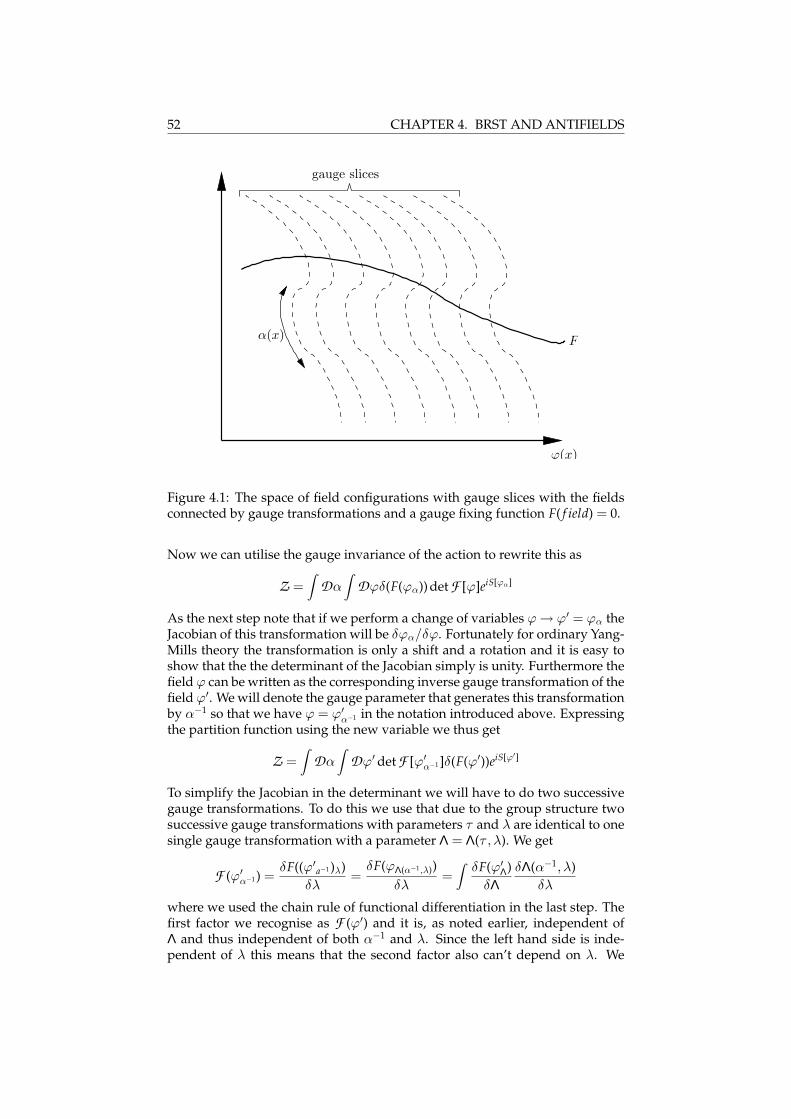
52 CHAPTER 4. BRST AND ANTIFIELDS
PSfrag replacements
α(x)F (ϕ) = 0
gauge slices
ϕ(x)
Figure 4.1: The space of field configurations with gauge slices with the fieldsconnected by gauge transformations and a gauge fixing function F( f ield) = 0.
Now we can utilise the gauge invariance of the action to rewrite this as
Z =Z
DαZ
Dϕδ(F(ϕα)) det F [ϕ]eiS[ϕα]
As the next step note that if we perform a change of variables ϕ→ ϕ′ = ϕα theJacobian of this transformation will be δϕα/δϕ. Fortunately for ordinary Yang-Mills theory the transformation is only a shift and a rotation and it is easy toshow that the the determinant of the Jacobian simply is unity. Furthermore thefield ϕ can be written as the corresponding inverse gauge transformation of thefield ϕ′. We will denote the gauge parameter that generates this transformationby α−1 so that we have ϕ = ϕ′α−1 in the notation introduced above. Expressingthe partition function using the new variable we thus get
Z =Z
DαZ
Dϕ′ det F [ϕ′α−1 ]δ(F(ϕ′))eiS[ϕ′]
To simplify the Jacobian in the determinant we will have to do two successivegauge transformations. To do this we use that due to the group structure twosuccessive gauge transformations with parameters τ and λ are identical to onesingle gauge transformation with a parameter Λ = Λ(τ , λ). We get
F (ϕ′α−1 ) =δF((ϕ′a−1 )λ)
δλ=
δF(ϕΛ(α−1,λ))δλ
=Z
δF(ϕ′Λ)δΛ
δΛ(α−1, λ)δλ
where we used the chain rule of functional differentiation in the last step. Thefirst factor we recognise as F (ϕ′) and it is, as noted earlier, independent ofΛ and thus independent of both α−1 and λ. Since the left hand side is inde-pendent of λ this means that the second factor also can’t depend on λ. We
4.1. ANTIFIELDS AND THE MASTER ACTION 53
can however not say anything about its dependence on α−1. When taking thedeterminant of this we get a product of two determinants, and our partitionfunction takes the following form
Z =(Z
Dα detδΛ(α−1, λ)
δλ
)ZDϕ′δ(F(ϕ′) det F (ϕ′)eiS[ϕ′]
Note how the only α-dependence left is in δΛ/δλ which does not depend onthe field ϕ′ so that this factor could be brought outside of the ϕ′ integral and inthis way giving a simple constant. Of course this constant is really infinite sinceit corresponds to the integration along the gauge orbits. In matrix elementscalculations it will cancel as we have already explained. This however meansthat we get exactly the same physics by simply neglecting this extra factor andtaking the remaining functional integral as our fundamental partition function.This is what we will do know. What is left is
Z =Z
Dϕδ(F(ϕ)) det F (ϕ)eiS[ϕ]
Here the delta function stops the gauge invariance of the action from being aproblem. We are in reality only integrating along the gauge-fixed surface infield space.
When doing perturbation theory the form of the path integral we have arrivedat is not particularly convenient so we will have to rewrite it. One good thingabout the formula above is that it does not depend on the specific gauge fixingfunction you choose. This means that if we take F(ϕ) = f (ϕ)− ω, where f issome function and ω is a field, then Z will not depend on ω. If we then comeup with a function ρ(ω) so that
RDωρ(ω) = 1 this weight function can then be
used to integrate over Z without changing its value. I.e., we have
Z =Z
Dωρ(ω)Z =Z
DϕZ
Dωρ(ω)δ( f (ϕ)− ω) det F (ϕ)eiS[ϕ] =
=Z
Dϕρ( f (ϕ)) det F (ϕ)eiS[ϕ]
Now since we only know how to do functional integrals over gaussian inte-grands it is convenient to choose ρ in such a way: ρ(ω) = exp(− i
2ξ
Rdxω2). Here
ξ is an arbitrary constant. Strictly speaking we should include a normalisationconstant to ensure that ρ integrates to 1, but as constants cancels anyway whencalculating physical quantities we can ignore it. This exponential factor canthen be incorporated as a new term in the action. As the next step we rewritethe determinant as a functional integral over two new fermionic fields. Recallthat
RDbDc exp(i
RRbMc) is proportional to det M when c and b are fermionic.
The c-field is called a ghost and b goes under the name antighost. The modifiedFadeev-Popov action we end up with is
SFP = S−Z
dx1
2ξf 2(ϕ(x)) +
Zdy
Zdxb(y)
δ f (ϕλ(y)δλ(x)
c(x) (4.1)
We should note that there is another way to include the delta function in theaction, using its fourier expansion:
δ(F(ϕ)) ∼Z
DheihF(ϕ)
54 CHAPTER 4. BRST AND ANTIFIELDS
To utilise this a new auxiliary field h would have to be introduced and pathintegrated over. In fact this way of handling the delta function can be combinedwith the one that yielded the f 2-term by using the formula
ZDheih( ξ
2 h− f ) ∼ e−i
2ξ f 2
which can be derived by completing the square in the exponent. In this waythe action in equation (4.1) can be rewritten as
SFP = S +Z
dx(ξ
2h(x)− f (x))h(x) +
ZZdxdyb(y)
δ f (ϕλ(y)δλ(x)
c(x) (4.2)
As an example let us apply the Fadeev-Popov method to the case of SYM.The gauge transformations are as we know given by δAµ = ∂µα− [Aµ, α] andδχc = −[χc, α]. We can rewrite this in the form above in the following way ifwe expand the field in terms of the generators of the Lie algebra, Aµ = Ai
µTi,χc = χciTi and α = αiTi, and use the structure constants of the Lie algebra,[Ti, T j] = f i jkTk,
δAiµ(x) =
Zd10y(δi j∂µ − f k ji Ak
µ(x))δ(x− y)α j(y)
δχci(x) = −Z
d10y f k jiχckδ(x− y)α j(y)
The conventional gauge fixing condition is to choose f i(A) = ∂µAiµ. This means
that
f i(Aα) = ∂µAiµ +
Zd10y(δi j∂2 − f k ji∂µAk
µ(x)− f k ji Akµ(x)∂µ)δ(x− y)α j(y)
Taking the functional derivative we get
δ f i(Aα(x))δα j(y)
= (δi j∂2 − f k ji∂µAkµ(x)− f k ji Ak
µ(x)∂µ)δ(x− y)
so that the ghost term in the action becomesZ
d10yZ
d10xbi(x)(δi j∂2 − f k ji∂µAkµ(x)− f k ji Ak
µ(x)∂µ)δ(x− y)c j(y) =
=Z
d10xbi∂µ∇µci = trZ
d10xb∂µ∇µc
Note that the ghost field c has to belong to the same representation as the gaugeparameter but with the opposite statistics. The antighost should be a field thatis dual to the gauge fixing condition f (a vector if f is a vector and a cospinorif f is a spinor etc), again with the opposite Grassmann parity. The completeFadeev-Popov action for SYM becomes
SFP = trZ
d10x[−1
4Fµν Fµν − 1
2ξ∂µAµ∂ν Aν +
i2χγρ∇ρχ + b∂µ∇µc
]
using the form in equation (4.1). The gauge transformation of the ghost fieldsis given directly by the fact that they are Lie algebra valued. There is no longer
4.1. ANTIFIELDS AND THE MASTER ACTION 55
any gauge invariance though, because of the gauge fixing term. One negativething with the Fadeev-Popov action is that it is no longer invariant under thesupersymmetry transformations. This is easy to see by computing the variationof the added terms. The situation here is comparable to what happens whenyou choose a non-covariant gauge fixing — then manifest Lorentz symmetryis lost. Here the problem is that when choosing a gauge the way we do super-symmetry goes away. The c-ghost introduced here is the same one as we earlierfound at the lowest θ and λ-level when doing the pure spinor expansion. Thiswill become apparent in a short while.
4.1.2 BRST-quantisation
One drawback of the Fadeev-Popov method is that it does not yield the rightresult in all cases. It does work for abelian and non-abelian Yang-Mills theoryso it covers the cases we are interested in. There are however more generaltypes of gauge theories where something else is necessary. In particular this isthe case for
1. reducible theories (there is gauge invariance in the gauge parameter)
2. open gauge algebras (i.e. it is only an algebra on-shell)
In addition to these limitations not all gauges will yield a correct result withthe Fadeev-Popov procedure. To generalise the Fadeev-Popov result so that itis valid for other cases the key point is to observe that the Fadeev-Popov ac-tion has a new global symmetry that didn’t exist in the original action. Thisnew symmetry is the BRST-symmetry (named after Becchi, Rouet, Stora andTyutin). It involves a fermionic transformation of the fields — that is the pa-rameter of the transformation is a fermionic constant which we will denote byθ. It is convenient to introduce the BRST-operator s in the following way
δBRST A = (sA)θ
Note that this definition means that s will be acting from the right:
s(AB) = A(sB) + (−1)B(sA)B
This turns out to be convenient as it avoids some extra signs later on.
For the case of SYM s is given by
sAµ =∇µcsχc = χc, c
on the fields. This is just a gauge transformation with the ghost as gauge pa-rameter. On the ghosts on the other hand we have
sc = −12c, c
sb = −h
56 CHAPTER 4. BRST AND ANTIFIELDS
and on the auxiliary fieldsh = 0
The BRST-transformation has the peculiar property that it is nilpotent, s2 = 0.This is easy to verify from the definitions above with frequent use of the Jacobiidentity. The gauge fixed action is of the form SFP = S + Sextra where S is theoriginal action that has no dependence on the ghost or the auxiliary field (it iseasiest to work with the form of the action in equation (4.2)). All fields of thiskind appear in the extra terms in Sextra. Since the BRST-transformation of theoriginal fields is just a gauge transformation (albeit with a peculiar parameter)it is trivial that S is invariant under s, sS = 0. To show that the same is true forSextra we first note that we can rewrite the integrand of this part of the action as
(ξ
2h− ∂µAµ)h + b∂µ∇µc = s(b∂µAµ − ξ
2bh)
Now the nilpotency immediately tells us that also Sextra and thus the entireFadeev-Popov action is BRST-invariant.
To describe the BRST-symmetry in some more generality we will first intro-duce a compact notation that in this case is quite useful. In this so called DeWitt notation we will let integration over space-time be implied by summationover indices. As an example AµBµ should be taken to mean
RdxAµ(x)Bµ(x) in
ordinary notation. In this way a general gauge transformation can be written
δαϕi = R[ϕ]iAαA
ϕi denotes all the fields in the theory and αA the gauge parameters. Gaugeinvariance of the action is now compactly written as δRS/δϕi R[ϕ]i
A = 0. Herewe introduced the right functional derivative δR/δϕk. It simply means thatthe field ϕk is “removed” towards the right when taking the derivative. It isimportant to keep track of this when we are dealing with a mixture of fermionicand bosonic quantities. There is of course a corresponding definition of a leftderivative. To write down the BRST-transformation of the ordinary fields wehave to introduce ghost fields, cA — one for every gauge parameter — and thenwe simply define
sϕi = R[ϕ]iAcA
Now the question is how s should act on the ghosts. The interesting property ofthe BRST-transformation for the Yang-Mills case really was that it was nilpotentso we will demand the same for the general case:
0 = s2ϕi = s(R[ϕ]iAcA) = Ri
AscA + (−1)A+1 δR RiA
δϕk (sϕk)cA =
= RiAscA + (−1)A+1 δR Ri
Aδϕk Rk
BcBcA
⇔
RiAscA = (−1)A 1
2
(δR RiA
δϕk RkB + (−1)(A+1)(B+1) δR Ri
Bδϕk Rk
A
)cBcA
Here it is perhaps worth pointing out that when an index such as A or B ap-pears over−1 we mean the Grassmann parity of the gauge parameter αA. This
4.1. ANTIFIELDS AND THE MASTER ACTION 57
is why we have to write A + 1 etc. to get the parity of the ghost cA. To fulfillthis equation we should take scA to be given by
scA =12
TABC[ϕ]cCcB
where T is defined by
δR RiB
δϕk RkC + (−1)(B+1)(C+1) δR Ri
C
δϕk RkB = Ri
ATABC + · · ·
This is the commutation relation of a general gauge algebra. You would findthis expression if you tried to compute the commutator of two gauge transfor-mations: [δα1 , δα2 ]ϕk. For the case of a closed algebra there are no more termson the right hand side, but for open algebras you also have a term propor-tional to the equation of motion. For instance for Yang-Mills theory this wouldbe equivalent to the Lie algebra commutation relation and T would really begiven by the structure constants of the Lie algebra. The definition of scA wehave presented does actually only work for the case of closed algebras. Openalgebras can be handled but requires extra complications so we will restrictourselves to the closed case. With the definition of s we have given, you willalso have nilpotency when acting on c. To show this you only need to use thatT satisfy the analogous thing of a Jacobi identity. This far we have been able tointroduce a nilpotent BRST-operator, but we have seen no sign of the antighostand the auxiliary field. The BRST-transformation of the fields and the ghostsonly includes these two types of fields themselves so there is no apparent needfor anything else. However we can alway introduce so called trivial pairs offields if we let s act on them in the following way
sA = BsB = 0
In this way the fact that s2 = 0 on A and B is trivial. By comparing with theexample of Yang-Mill theory that we presented above we see that the antighostbA and the auxiliary field hB are of precisely this kind
sbA = hA
shA = 0
Exactly why we need this trivial pair will be demonstrated shortly. First we willgo on to the next step after s has been completely defined — that of constructinga BRST-invariant action. The new action we wish to have should of coursehave some resemblance to the original action we start from. It is for instancereasonable to demand that if we put all new fields to zero the modified actionshould reduce to the old one. This can be achieved by the following split
Smod = S + Snew
Exactly as for Yang-Mills the gauge invariance of the ordinary action S impliesthat it is also BRST-invariant. Now the question is how to construct a functionalSnew of all the fields that is BRST-invariant. For the case of Yang-Mills this
58 CHAPTER 4. BRST AND ANTIFIELDS
term was of the form s(something). This is in fact the general solution. It canbe shown that every BRST-invariant action can be written on the form gaugeinvariant functional of only the ordinary field plus s on functional of all thefields, see [17] for a proof. So Snew has to be of the form sΨ if it is to satisfysSnew = 0. Since s is fermionic the same has to be true for the functional Ψ tomake sure that the action is bosonic. To further investigate the properties of Ψis is useful to introduce a new grading, the ghost number. Ordinary fields areno ghosts so we will assign them ghost number zero, gh(ϕ) = 0, and since theghosts are ghosts they have to have ghost number one, gh(c) = 1. By lookingat the Fadeev-Popov action for Yang-Mills and assuming that it is purely ofghost number zero we see that gh(h) has to be zero (because of the h2-term)and gh(b) = −1 (because of the b∂∂c-term). Now make note of the fact thatthe operator s always increases ghost number by one unit. This means that thefermion Ψ has to have ghost number equal to -1 if we want gh(Snew) to vanish.It is now apparent why we had to introduce the trivial pair of the antighost andthe auxiliary field — otherwise it would have been impossible to construct afunctional with ghost number -1. It could not have been done with only ϕ andc since they both have non-negative ghost numbers.
The BRST-procedure [18] really only says that we should construct an actionthat is invariant under BRST-symmetry (and other globals symmetries of theoriginal action) and then use this action for all computations. For Yang-Millswe can see that choosing the fermion Ψ in an appropriate way we will alwaysgive us back the FP-action and so in this case the BRST-method obviously givesa correct gauge fixed action for the gauge theory we started from. But whatabout other choices for Ψ? Do we have to put restrictions on the way to chooseΨ? The answer is that under certain conditions to be explained shortly thechoice of Ψ does not matter as amplitudes computed with the BRST-actionwill be completely independent of the choice of Ψ. In fact we can considerdifferent Ψs to correspond to different ways of fixing the gauge. Some Ψs givethe same result as the Fadeev-Popov procedure, but others do not so we dohave a greater generality here. For the independence on Ψ to come true wehave to restrict the set of operators we are allowed to calculate matrix elementsfor. Recall that with the ordinary gauge invariant action we are only interestedin gauge invariant operators since they are the only ones that are measurable.Now that we in addition to the ordinary fields also have an assortment of ghostetc to construct operators with there is obviously need for a generalisation.The key is to define observables to be operators with ghost number zero thatsatisfy sO = 0. Indeed if O only depends on ϕ this reduces to demanding gaugeinvariance. We also have to define which of the states in the now enlargedHilbert space are physical. To do this we assume that it is possible to introducea generator for the BRST-transformation: sO = [Q,O. Then physical statevectors are defined by Q |V〉 = 0. It is now easy to show that it is precisely formatrix elements of physical operators between physical states that Ψ can bechosen at will. Indeed upon a change Ψ→Ψ + δΨ the matrix element 〈α|O |β〉
4.1. ANTIFIELDS AND THE MASTER ACTION 59
changes by
i 〈α|OiZ
sΨ |β〉 = iZ〈α|OQ,Ψ |β〉 =
= iZ〈α|OQΨ |β〉+ i
Z〈α|OΨ Q |β〉︸ ︷︷ ︸
=0
=
= iZ〈α| [O , Q︸ ︷︷ ︸
=0
Ψ |β〉 ± iZ〈α|Q︸ ︷︷ ︸
=0
OΨ |β〉 = 0
where both the O and the states are assumed to be physical. Operators onthe form sP trivially satisfy the physicality condition but their matrix elementsvanish for physical states: 〈α| sP |β〉 = 〈α|QP |β〉 ± 〈α|P Qκ |β〉 = 0. Further-more it follows from s2 = 0 that Q2 = 0 so that states on the form Q |γ〉 alsoare trivially physical. Also in this case matrix elements vanish: 〈α|OQ |γ〉 =〈α| [Q,O |γ〉 ± 〈α|QO |γ〉 = 0. Physical observables and physical states couldthus really be said to live in the cohomology of s and Q respectively.
4.1.3 BV-quantisation
For closed algebras the application of the BRST-procedure is very straightfor-ward as demonstrated above. But for open algebras things are more compli-cated. By following the antifield procedure of Batalin and Vilkovisky we willreach exactly the same goal of a BRST invariant action, but in a more systematicway. In short this method consists of three steps
1. Introduce antifields.
2. Solve the master equation with boundary conditions to give the masteraction.
3. Gauge fix the master action.
Of course we will have to define what each step means in some more detail butthe end result is that the gauge fixed master action is the BRST-invariant actionwe are looking for. A nice introduction to the BV-formalism is the review [19],the short paper [20] and chapter 15 of [17]. There is also the comprehensiveand mathematical book [21].
Let us start by defining the fields we are working with. First of all we haveto introduce the ghost fields in the same way as earlier. To be able to referto both the ordinary fields and the ghosts in a compact way we introduce thegeneral field ΦI = (ϕi, cA). Now we introduce for both the ordinary field ϕ andthe ghost c a corresponding antifield. They will denoted by a ∗: ϕ∗i and c∗A, orin short Φ∗
I . The antifield Φ∗I will be defined to have the opposite Grassmann
parity of ΦI and its ghost number will be gh(Φ∗I ) = −gh(ΦI)− 1. The antifield
of the ghost should not be confused with the antighost as they are not the same.

60 CHAPTER 4. BRST AND ANTIFIELDS
We will now go on to define the master equation and to do this we first haveto introduce the antibracket. This is a bilinear bracket that acts on functionalsof the fields and antifield in much the same way as the Poisson bracket acts onfunctionals of fields and their conjugate momenta. The definition is
(A, B) =δR AδΦI
δL BδΦ∗
I− δR A
δΦ∗I
δL BδΦI (4.3)
Note that just like the Poisson bracket satisfy ϕi, π jPB ∼ δij the antibracket
satisfy (ΦI ,Φ∗J ) = δ I
J so in some sense the fields and antifields can be said tobe conjugate to each other. The symmetry properties of the antibracket arehowever not the same as for the Poisson bracket. The most noteworthy thingis the following
(A, B) = −(−1)(A+1)(B+1)(B, A)
So for two bosonic functionals the bracket is symmetric while in all other casesit is antisymmetric. Note from the definition that the bracket is fermionic andalways increases the ghost number by one unit.
We are now ready to introduce the (classical) master equation:
(S,S) = 0 (4.4)
If we assume that the functional S is bosonic we can use the definition ofthe bracket and the relation between left and right functional derivatives1 torewrite this as
δLSδΦI
δLSδΦ∗
I= 0
The master action, S, will be required to be a solution of this equation with zeroghost number and as the name implies it will have something to do with theaction. To make contact with the gauge theory of our choice we must requirethat if we put all the antifields to zero we get back the usual action, S(Φ,Φ∗ =0) = S(Φ). We will actually need to impose more “boundary” conditions sinceotherwise the action S itself would be a solution due to it not depending onany antifields and this solution would obviously not be very interesting sinceit does not provide anything new. We will not dwell on this extra condition,but one can show that in S there are gauge invariances and what the conditionsays is roughly that the number of these has to equal them number of antifields.A solution satisfying these condition is called a proper solution. We can invery much the same way as for the BRST procedure introduce new variablesas trivial pairs if we to the master action add terms of the following kind S0 +hAb∗A. It is trivial that such terms does not alter the fact that (S,S) = 0. Inthis way antighosts, auxiliary fields and their corresponding antifields can beadded to the set of available fields, ΦI and Φ∗
I .
A remarkable feature of the master action is that it encodes all informationabout the gauge structure of the theory. This can be seen by expanding S interms of the number of antifield: S = S + S1 + S2 + · · · . The master equation
1When acting on objects that are not algebra valued or similarly we have δL Aδ I
Φ= (−1)(A−I)I δR A
δΦI
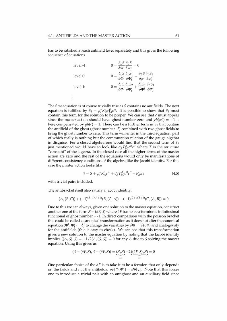
4.1. ANTIFIELDS AND THE MASTER ACTION 61
has to be satisfied at each antifield level separately and this gives the followingsequence of equations
level -1: 0 =δLSδΦI
δLSδΦ∗
I= 0
level 0: 0 =δLSδΦI
δLS1
δΦ∗I
=δLSδϕi
δLS1
δϕ∗i
level 1: 0 =δLSδΦI
δLS2
δΦ∗I
+δLS1
δΦIδLS1
δΦ∗I
...
The first equation is of course trivially true as S contains no antifields. The nextequation is fulfilled by S1 = ϕ∗i R[ϕ]i
AcA. It is possible to show that S1 mustcontain this term for the solution to be proper. We can see that c must appearsince the master action should have ghost number zero and gh(ϕ∗i ) = −1 ishere compensated by gh(c) = 1. There can be a further term in S1 that containthe antifield of the ghost (ghost number -2) combined with two ghost fields tobring the ghost number to zero. This term will enter in the third equation, partof which really is nothing but the commutation relation of the gauge algebrain disguise. For a closed algebra one would find that the second term of S1just mentioned would have to look like c∗ATA
BCcBcC where T is the structure“constant” of the algebra. In the closed case all the higher terms of the masteraction are zero and the rest of the equations would only be manifestations ofdifferent consistency conditions of the algebra like the Jacobi identity. For thiscase the master action looks like
S = S + ϕ∗i RiAcA + c∗ATA
BCcBcC + b∗AhA (4.5)
with trivial pairs included.
The antibracket itself also satisfy a Jacobi identity:
(A, (B, C)) + (−1)(B+1)(A+1)(B, (C, A)) + (−1)(C+1)(B+1)(C, (A, B)) = 0
Due to this we can always, given one solution to the master equation, constructanother one of the form S + (δF,S) where δF has to be a fermionic infinitesimalfunctional of ghostnumber = -1. In direct comparison with the poisson bracketthis could be called a canonical transformation as it does not alter the canonicalequation (ΦI ,Φ∗
J ) = δ IJ to change the variables by δΦ = (δF,Φ) and analogously
for the antifields (this is easy to check). We can see that this transformationgives a new solution to the master equation by noting that the Jacobi identityimplies ((A,S),S) = ±1/2(A, (S,S)) = 0 for any A due to S solving the masterequation. Using this gives us
(S + (δF,S),S + (δF,S)) = (S,S)︸ ︷︷ ︸=0
−2 ((δF,S),S)︸ ︷︷ ︸=0
= 0
One particular choice of the δF is to take it to be a fermion that only dependson the fields and not the antifields: δF[Φ,Φ∗] = εΨ[ϕ]. Note that this forcesone to introduce a trivial pair with an antighost and an auxiliary field since

62 CHAPTER 4. BRST AND ANTIFIELDS
otherwise there is no way to get the desired ghost number of minus one. Us-ing the definition of the antibracket shows us that the corresponding changein S is δS = (εΨ,S) = ε δRΨ
δΦIδLSδΦ∗
I= ε δLΨ
δΦIδRSδΦ∗
I. We can interpret this as an in-
finitesimal change of variables: S → S ′[Φ,Φ∗] = S[Φ,Φ∗ + ε δLΨδΦ ]. The infinites-
imal transformation can be integrated to yield the finite field transformationΦ∗
I → Φ′∗I = Φ∗
I + δLΨδΦI . The utility of this particular transformation will become
clearer in a short while.
There is another very important consequence of the fact that (A, (S,S)) = 0 andthat is that because of this we can utilise the bracket to define an operator thatis guaranteed to be nilpotent. This operator, the generalised BRST-operator, isgiven by sO = (O ,S). Applying this to the fields we find
sΦI = (ΦI ,S) =δLSδΦ∗
I
In this sense the antifields can be said to be the generators of the BRST-trans-formation. This is certainly the case when the master action is linear in the anti-fields and closed gauge algebras is a particular example. It is easy to see fromthe action in (4.5) that here the generalised BRST-transformation of the fieldsexactly matches the one defined in the previous part. The antifields transformas
sΦ∗I = (Φ∗
I ,S) = − δLSδΦI
It is quite remarkable that in the BV-formulation one single object encodes allinformation about both the gauge structure and the BRST-transformation for agauge theory.
As we noted there exists gauge symmetries in the master action so it is, as itstands, unsuitable to use as an action for path integral calculation. It is indeedvery easy to demonstrate the existence of these gauge invariances — all youhave to do is to take a derivative of the master equation
0 =δL
δΦI
( δLSδΦJ
δLSδΦ∗
J
)=
( δL
δΦIδLSδΦJ
) δLSδΦ∗
J+ (−1)J I δLS
δΦJ
( δL
δΦIδLSδΦ∗
J
)=
=( δL
δΦIδLSδΦJ
) δLSδΦ∗
J+
( δL
δΦIδLSδΦ∗
J
) δLSδΦJ
This shows that the variation of the action is zero for the transformations
δΛΦJ = ΛI δL
δΦIδLSδΦ∗
J
δΛΦ∗J = ΛI δL
δΦIδLSδΦJ
(4.6)
By taking a derivative with respect to an antifield instead we also find the fol-lowing gauge invariances
δ ′ΩΦJ = (−1)JΩIδL
δΦ∗I
δLSδΦ∗
J
δ ′ΩΦ∗J = ΩI
δL
δΦ∗I
δLSδΦJ
(4.7)
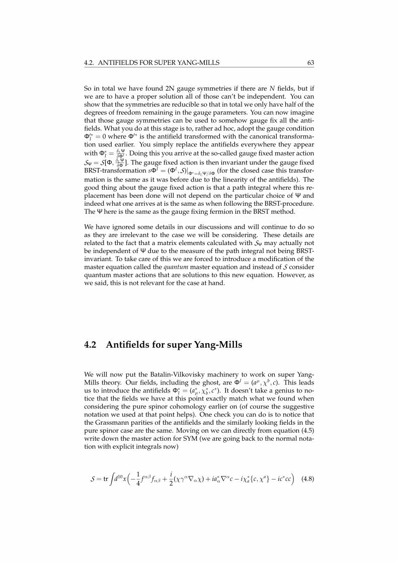
4.2. ANTIFIELDS FOR SUPER YANG-MILLS 63
So in total we have found 2N gauge symmetries if there are N fields, but ifwe are to have a proper solution all of those can’t be independent. You canshow that the symmetries are reducible so that in total we only have half of thedegrees of freedom remaining in the gauge parameters. You can now imaginethat those gauge symmetries can be used to somehow gauge fix all the anti-fields. What you do at this stage is to, rather ad hoc, adopt the gauge conditionΦ′∗
I = 0 where Φ′∗ is the antifield transformed with the canonical transforma-tion used earlier. You simply replace the antifields everywhere they appearwith Φ∗
I = δLΨδΦI . Doing this you arrive at the so-called gauge fixed master action
SΨ = S[Φ, δLΨδΦ ]. The gauge fixed action is then invariant under the gauge fixed
BRST-transformation sΦI = (ΦI ,S)|Φ∗=δLΨ/δΦ (for the closed case this transfor-mation is the same as it was before due to the linearity of the antifields). Thegood thing about the gauge fixed action is that a path integral where this re-placement has been done will not depend on the particular choice of Ψ andindeed what one arrives at is the same as when following the BRST-procedure.The Ψ here is the same as the gauge fixing fermion in the BRST method.
We have ignored some details in our discussions and will continue to do soas they are irrelevant to the case we will be considering. These details arerelated to the fact that a matrix elements calculated with SΨ may actually notbe independent of Ψ due to the measure of the path integral not being BRST-invariant. To take care of this we are forced to introduce a modification of themaster equation called the quantum master equation and instead of S considerquantum master actions that are solutions to this new equation. However, aswe said, this is not relevant for the case at hand.
4.2 Antifields for super Yang-Mills
We will now put the Batalin-Vilkovisky machinery to work on super Yang-Mills theory. Our fields, including the ghost, are ΦI = (aµ, χb, c). This leadsus to introduce the antifields Φ∗
I = (a∗µ, χ∗b , c∗). It doesn’t take a genius to no-tice that the fields we have at this point exactly match what we found whenconsidering the pure spinor cohomology earlier on (of course the suggestivenotation we used at that point helps). One check you can do is to notice thatthe Grassmann parities of the antifields and the similarly looking fields in thepure spinor case are the same. Moving on we can directly from equation (4.5)write down the master action for SYM (we are going back to the normal nota-tion with explicit integrals now)
S = trZ
d10x(−1
4f αβ fαβ +
i2
(χγα∇αχ) + ia∗α∇αc− iχ∗ac, χa− ic∗cc)
(4.8)
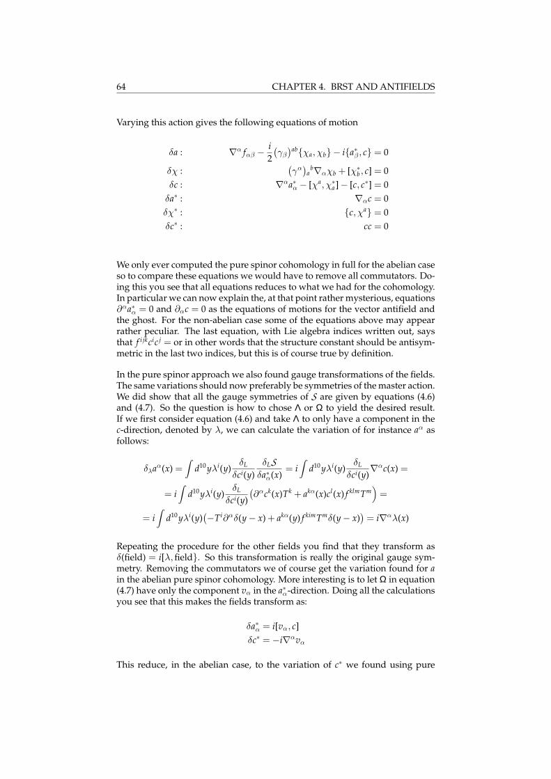
64 CHAPTER 4. BRST AND ANTIFIELDS
Varying this action gives the following equations of motion
δa : ∇α fαβ − i2(γβ
)abχa, χb− ia∗β , c = 0
δχ :(γα
)a
b∇αχb + [χ∗b , c] = 0δc : ∇αa∗α − [χa, χ∗a]− [c, c∗] = 0
δa∗ : ∇αc = 0δχ∗ : c, χa = 0δc∗ : cc = 0
We only ever computed the pure spinor cohomology in full for the abelian caseso to compare these equations we would have to remove all commutators. Do-ing this you see that all equations reduces to what we had for the cohomology.In particular we can now explain the, at that point rather mysterious, equations∂αa∗α = 0 and ∂αc = 0 as the equations of motions for the vector antifield andthe ghost. For the non-abelian case some of the equations above may appearrather peculiar. The last equation, with Lie algebra indices written out, saysthat f i jkcic j = or in other words that the structure constant should be antisym-metric in the last two indices, but this is of course true by definition.
In the pure spinor approach we also found gauge transformations of the fields.The same variations should now preferably be symmetries of the master action.We did show that all the gauge symmetries of S are given by equations (4.6)and (4.7). So the question is how to chose Λ or Ω to yield the desired result.If we first consider equation (4.6) and take Λ to only have a component in thec-direction, denoted by λ, we can calculate the variation of for instance aα asfollows:
δλaα(x) =Z
d10yλi(y)δL
δci(y)δLS
δa∗α(x)= i
Zd10yλi(y)
δL
δci(y)∇αc(x) =
= iZ
d10yλi(y)δL
δci(y)(∂αck(x)Tk + akα(x)cl(x) f klmTm
)=
= iZ
d10yλi(y)(−Ti∂αδ(y− x) + akα(y) f kimTmδ(y− x)
)= i∇αλ(x)
Repeating the procedure for the other fields you find that they transform asδ(field) = i[λ,field. So this transformation is really the original gauge sym-metry. Removing the commutators we of course get the variation found for ain the abelian pure spinor cohomology. More interesting is to let Ω in equation(4.7) have only the component vα in the a∗α-direction. Doing all the calculationsyou see that this makes the fields transform as:
δa∗α = i[vα, c]δc∗ = −i∇αvα
This reduce, in the abelian case, to the variation of c∗ we found using pure
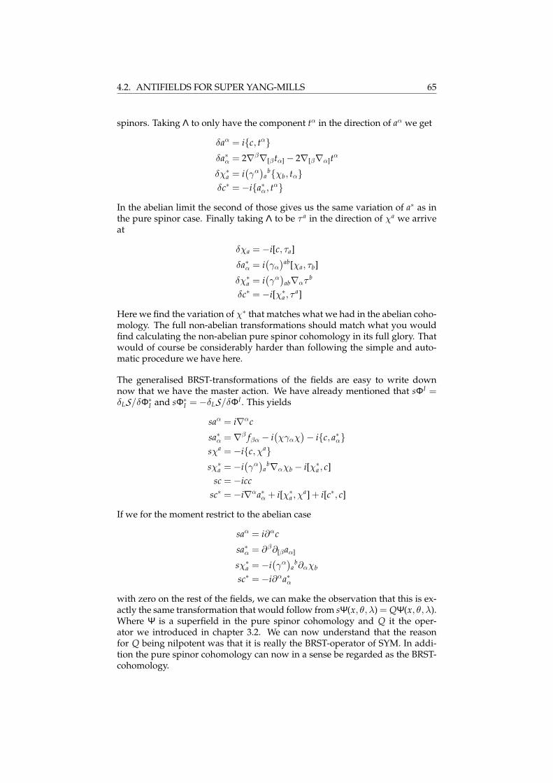
4.2. ANTIFIELDS FOR SUPER YANG-MILLS 65
spinors. Taking Λ to only have the component tα in the direction of aα we get
δaα = ic, tαδa∗α = 2∇β∇[β tα] − 2∇[β∇α]tα
δχ∗a = i(γα
)a
bχb, tαδc∗ = −ia∗α, tα
In the abelian limit the second of those gives us the same variation of a∗ as inthe pure spinor case. Finally taking Λ to be τ a in the direction of χa we arriveat
δχa = −i[c, τa]
δa∗α = i(γα
)ab[χa, τb]
δχ∗a = i(γα
)ab∇ατ b
δc∗ = −i[χ∗a , τa]
Here we find the variation of χ∗ that matches what we had in the abelian coho-mology. The full non-abelian transformations should match what you wouldfind calculating the non-abelian pure spinor cohomology in its full glory. Thatwould of course be considerably harder than following the simple and auto-matic procedure we have here.
The generalised BRST-transformations of the fields are easy to write downnow that we have the master action. We have already mentioned that sΦI =δLS/δΦ∗
I and sΦ∗I = −δLS/δΦI . This yields
saα = i∇αc
sa∗α =∇β fβα − i(χγαχ
)− ic, a∗αsχa = −ic, χasχ∗a = −i
(γα
)a
b∇αχb − i[χ∗a , c]sc = −icc
sc∗ = −i∇αa∗α + i[χ∗a , χa] + i[c∗, c]
If we for the moment restrict to the abelian case
saα = i∂αc
sa∗α = ∂β∂[βaα]
sχ∗a = −i(γα
)a
b∂αχb
sc∗ = −i∂αa∗α
with zero on the rest of the fields, we can make the observation that this is ex-actly the same transformation that would follow from sΨ(x, θ, λ) = QΨ(x, θ, λ).Where Ψ is a superfield in the pure spinor cohomology and Q it the oper-ator we introduced in chapter 3.2. We can now understand that the reasonfor Q being nilpotent was that it is really the BRST-operator of SYM. In addi-tion the pure spinor cohomology can now in a sense be regarded as the BRST-cohomology.

66 CHAPTER 4. BRST AND ANTIFIELDS
Chapter 5
Conclusions
We have in this thesis showed how super Yang-Mills theory can be formu-lated using the concept of pure spinors and how this formulation has the niceproperty of automatically also including ghosts and antifields in the theory.We have however not said anything about how this new formulation mightbe useful. In the introduction to chapter 3 we briefly mentioned that the purespinor approach was introduced in conjunction with the Green-Schwarz su-perstring. In fact if we quantise the superparticle, which really is nothing butthe zero mode of the GS superstring, we will as a result get a wavefunction thatsatisfy all the equations of SYM. This quantisation has however always beenplagued with the problem that it is not known how to do it covariantly whileit can easily be done in the light-cone. Berkovits showed that the superparticlecan be reformulated by including pure spinors in the action and in an ad-hocway imposing the Q = 0 constraint. This does not really solve the problemof covariant quantisation as manifest Lorentz invariance appears to have to bebroken to show the equality of the new and old formulation. However, whenextended to the superstring, the pure spinor formulation turns out to be usefulwhen calculating scattering amplitudes.
Another interesting subject that we have overlooked is that of Berkovits’s ac-tion. We wrote down the BV-action for SYM in equation (4.8) directly in termsof the component fields. It would of course be interesting if one could some-how rewrite this in terms of the superfield Ψ = C(x, θ) + λa Aa(x, θ) + · · · itself.Berkovits has suggested a way of doing this that involves a very peculiar mea-sure. This measure is based on the fact that there exist a scalar in a product of5 θs and 3 λs.
Additional we have not had time to consider the relationship between the purespinor formalism and the spinorial cohomology introduced in [7, 8]. Therethe constraints of the superspace formulation of SYM are relaxed and a set offields resembling the one in Berkovits cohomology is found. It would also havebeen interesting to consider what happens if you allow fields that are not onlyrestricted to positive powers of the pure spinor λ.
67

68 CHAPTER 5. CONCLUSIONS
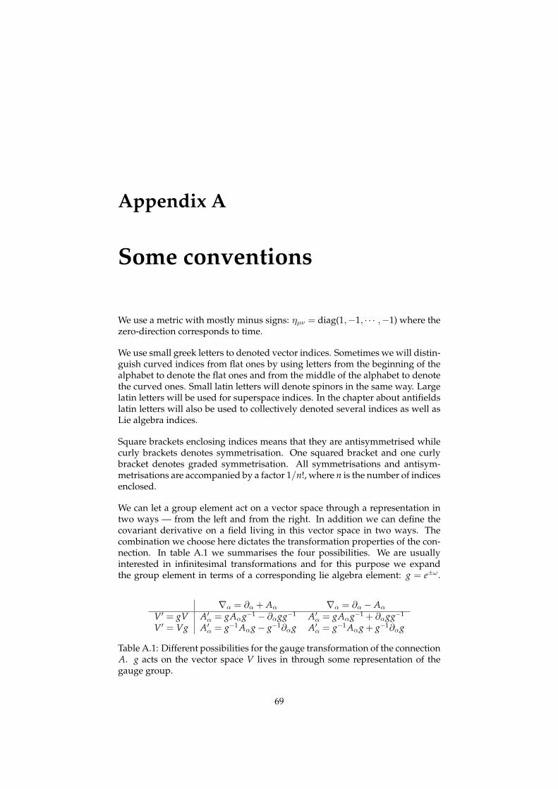
Appendix A
Some conventions
We use a metric with mostly minus signs: ηµν = diag(1,−1, · · · ,−1) where thezero-direction corresponds to time.
We use small greek letters to denoted vector indices. Sometimes we will distin-guish curved indices from flat ones by using letters from the beginning of thealphabet to denote the flat ones and from the middle of the alphabet to denotethe curved ones. Small latin letters will denote spinors in the same way. Largelatin letters will be used for superspace indices. In the chapter about antifieldslatin letters will also be used to collectively denoted several indices as well asLie algebra indices.
Square brackets enclosing indices means that they are antisymmetrised whilecurly brackets denotes symmetrisation. One squared bracket and one curlybracket denotes graded symmetrisation. All symmetrisations and antisym-metrisations are accompanied by a factor 1/n!, where n is the number of indicesenclosed.
We can let a group element act on a vector space through a representation intwo ways — from the left and from the right. In addition we can define thecovariant derivative on a field living in this vector space in two ways. Thecombination we choose here dictates the transformation properties of the con-nection. In table A.1 we summarises the four possibilities. We are usuallyinterested in infinitesimal transformations and for this purpose we expandthe group element in terms of a corresponding lie algebra element: g = e±ω .
∇α = ∂α + Aα ∇α = ∂α − Aα
V′ = gV A′α = gAαg−1 − ∂αgg−1 A′
α = gAαg−1 + ∂αgg−1
V′ = Vg A′α = g−1 Aαg− g−1∂αg A′
α = g−1 Aαg + g−1∂αg
Table A.1: Different possibilities for the gauge transformation of the connectionA. g acts on the vector space V lives in through some representation of thegauge group.
69
70 APPENDIX A. SOME CONVENTIONS
Once again there are two choices. On ordinary fields we will let the groupelement act from the left and the covariant derivative with a minus which cor-responds to the upper right entry in table A.1. With this convention the in-finitesimal transformation of A becomes A′
α = A± [ω, Aα]± ∂αω. We want thederivative to have a positive sign so we have to chose g = e+ω and thus getδAα = ∂αω + [ω, Aα]. The transformation of an endomorphism on the repre-sentation vector space must with our convention be F′ = gFg−1 and the covari-ant derivative∇αF = ∂αF− [Aα, F]. We get δAα =∇αω as expected. The fieldstrength is with our definitions Fαβ = ∂αAβ − δβ Aα − [Aα, Aβ].
When introducing the exterior derivative on superspace we will instead use aright action and a covariant derivative with a plus sign, but when looking atthe component level one will find that it all reduces to the above definition.
Our superspace derivative is Da = δa − i(γαθ)a∂α.
Appendix B
Spinors and γ-matrices inD=10
B.1 Spinors
When doing relativistic physics we are interested in representations of theLorentz algebra. The homogeneous Lorentz algebra is defined by the com-mutation relations :
[Jµν , Jρσ] = i(ηνρ Jµσ − ηµρ Jνσ − ηνσ Jµρ + ηµσ Jνρ) (B.1)
The simplest (non-trivial) representation is the ordinary defining vector repre-sentation.
The spinor representations can be constructed by finding matrices Γµ that sat-isfy a Clifford algebra:
Γµ,Γν = 2ηµν (B.2)
It is then easy to show that generators that satisfy (B.1) can be defined asJµν = i
4 [Γµ,Γν ]. One can show that for a given dimension there is only onerepresentation of the Clifford algebra and it can be chosen to be unitary. Thatthere is only one representation means that if we can find two sets of (non-trivial) matrices that satisfy (B.2) they must be related by a similarity trans-formation: Γ′ = MΓM−1. That the representation can be chosen to be unitarymeans that a given set of Γ-matrices can be similarity transformed so that theysatisfy Γµ(Γµ)† = 1 (no summation). We will from now on assume that we havemade this choice.
By taking the transpose, complex conjugation and hermitian conjugation ofequation (B.2) we find that if Γµ gives a Clifford algebra so does (Γµ)T, (Γµ)∗
and (Γµ)†. Because of the uniqueness of the representation as stated above we
71
72 APPENDIX B. SPINORS AND γ-MATRICES IN D=10
can then find matrices so that
(Γµ)† = AΓµA−1
(Γµ)∗ = BΓµB−1
(Γµ)T = CΓµC−1
(B.3)
The similarity transformations A, B and C are not unrelated. By using that† = ∗T = T∗, T = †∗ = ∗† and ∗ = †T = T† one can derive the following sixidentities:
A ∼ C∗B A ∼ C†B A ∼ B†C (B.4)
C ∼ BT A B ∼ A∗C C ∼ A∗B (B.5)
As an example we have AΓµA−1 = (Γµ)† = (Γµ)∗T = (BΓµB−1)T =(B−1)TCΓµ((B−1)TC)−1. From this we can deduce that A ∼ (B−1)TC which isequivalent to the first relation in (B.5). It follows from the equations above thatC∗ ∼ C†⇔ C∼ CT (upper left and upper middle), B∗B∼ 1 (upper left and lowerright), A∗A∗ ∼ 1 ⇔ AA ∼ 1 (lower middle and lower right) and that A ∼ A†
(upper middle and lower left together with B∗B ∼ 1).
The existence of the similarity transformations in (B.3) enables us to create realLorentz invariant scalars. The transformation properties of a spinor s in thespace S that the Γ-matrices act on is such that it transform under Lorentz trans-formations as s→ (1 + iωµν Jµν )s. Here ω are the infinitesimal parameters of thetransformation. Now consider instead t = t†A. This object must transform as
t → t†(1 + iωµν Jµν )†A = t†(1− iωµν
−i4
[(Γν )†, (Γµ)†])
A =
= t†A(1− iωµν Jµν
)= t
(1− iωµν Jµν
)
where we used (B.3) to move A past the Γ-matrices in J. It is now obviousthat the bispinor ts is invariant under Lorentz transformations (at least to thefirst order in ω). It is possible to show that [Γµ, Jνρ] =
(Jνρvector
)µ
σΓσ . Because
of this we have that tΓµs and more generally tΓµ1 · · ·Γµn s transform as Lorentztensors.
The Grassmann algebra tells us that Γ0Γ0 = 1 and ΓiΓi = −1 (no summation)which together with the unitarity condition Γµ(Γµ)† = 1 (no summation) meansthat (Γ0)−1 = (Γ0)† = Γ0 and (Γi)−1 = (Γi)† = −Γi. Because of this we can takethe similarity transformation matrix A to be equal to Γ0 (note that this is com-patible with the equations AA ∼ 1 and A ∼ A† we had earlier). From now onwe will assume that this choice has been made. Since A now is a Γ-matrix it-self we can apply (B.3) on it so that we have A∗ = BAB−1 and AT = CAC−1.This together with the relations in (B.4) and (B.5) allows us to deduce thatB†B ∼ 1 (lower right and upper right). As the proportionality constant hasto be real and positive we might just as well normalise B so that it is one —that is B†B = 1.
We can now show that if we take t and s to be the same spinor in the com-binations above and only allow antisymmetrised products of Γ-matrices they
B.1. SPINORS 73
are either purely real or imaginary. This can be seen as follows: (sΓµ1···µn s)† =(1/n!)s†(Γ[µn )† · · · (Γµ1])†A†s = (1/n!)s†AΓ[µn · · ·Γµ1]s = (−1)n(n−1)/2 sΓµ1···µn s. Notethat this formula also works for the case n = 0. It is now easy to construct realbispinor terms to use in the action by multiplying with an i when appropriate.
The representation of the Clifford algebra will be 2d/2-dimensional when thenumber of spacetime dimensions d is even and 2(d−1)/2-dimensional when it isodd. In particular this means that in a 10-dimensional spacetime the spinorrepresentation constructed with the Γ-matrices will be 32-dimensional. Thisspinor representation is however not always irreducible. Consider the matrixΓ = Γ0 · · ·Γd. The square of this matrix is proportional to the unit matrix: ΓΓ =(−1)(d−1)+d(d−1)/2 (the first term in the exponent is due to ΓiΓi = −1 the otherterm comes from the anticommutations). Particularly in d = 10 we get a plussign on the right. Had we been working in a dimension that gave a minussign we would have to multiply Γ with an i in what follows. The matrix Γcan now be used to construct a projector. Any spinor can be decomposed ass = 1
2 (1 + Γ)s + 12 (1− Γ)s. The projection operators are P+ = 1
2 (1 + Γ) and P− =12 (1− Γ). They satisfy (P±)2 = P± and P+P− = P−P+ = 0. In this way the spaceof spinors S split into two subspaces S+ and S− each having half the dimensionof S. So in 10 spacetime dimension dim S± = 16. Note that this constructiononly is meaningful for even dimensions. I turns out that for d odd Γ is actuallyproportional to the identity itself. It is easy to show that [P±, Jµν ] = 0 whichmeans that J can be made block-diagonal by a suitable change of basis and thusthe original spinor representation is reducible. The two smaller representationsare called Weyl spinors and anti-Weyl spinors respectively. We will chose ourbasis so that s =
(s+
s−). The Γ-matrices themselves are not necessarily block
diagonal in such a basis. We have ΓΓµ = (−1)d−1ΓµΓ. In even dimensions theminus sign means that P+Γµs+ = ΓµP−s+ = 0 and P−Γµs+ = ΓµP+s+ = Γµs+
so here a Γ-matrix changes a Weyl spinor to an anti-Weyl and vice-versa. Thismeans that the Γ-matrices are block off-diagonal in our basis. We will denotethe off-diagonal blocks with a small γ: Γµ =
( 0 γµ
γµ 0
)Since A = Γ0 the product
AΓµ in tΓµs = t†AΓµs will be block diagonal and connect Weyl spinors withWeyl spinors and anti-Weyl spinors with anti-Weyl spinors. Writing out thedetails we have tΓµs = (t+)†γ0γµs+ + (t−)†γ0γµs−. From now on we will notwrite out neither the γ0, the γ0 nor the tilde on γµ. We will rather use the onesymbol γµ to denote the appropriate thing according to the context it appearsin. When between two Weyl spinors it should be assumed to really mean γ0γµ
etc. For instance the Grassmann like commutation relation γµ, γν = 2ηµν
should be interpreted as γµγν + γνγµ = 2ηµν or γµγν + γν γµ = 2ηµν .
In some cases the Weyl and anti-Weyl representations are further reducible. Re-call that C was a similarity transformation matrix that satisfied (Γµ)T = CΓµC−1.In ten spacetime dimensions it is possible to transform the Γ-matrices so thatC also can be taken to be Γ0. This is compatible with equations (B.4) and (B.5).It is then possible to consider the spinors that are such that s = s†A = sTC ourin other word spinors with real components: s∗ = s. These spinors form asubspace of all the spinors that is invariant under Lorentz rotations, they areknown as Majorana spinors. This way of choosing the Γ-matrices is known asthe real basis since it turns out that also the matrices themselves are real. To
74 APPENDIX B. SPINORS AND γ-MATRICES IN D=10
see this note that the first equation in (B.5) tells us that B is just proportional tounity now that C and A are equal, thus (Γµ)∗ = BΓµB−1 = Γµ. With Majoranaspinors we can do so called Majorana flips. Since tΓµ1···µn s is a scalar (in spinorspace), we should get back the same thing when we take the transpose of it:
tΓµ1···µn s =(tΓµ1···µn s
)T = −sT(Γµ1···µn )TCTt = −(−1)n(n−1)/2 sΓµ1···µn t (B.6)
Note how s and t have changed places. Here we did use that CT = (Γ0)T =Γ0Γ0(Γ0)−1 = Γ0. A tricky point is the minus that appears after the secondequality. It only appears if we assume that s and t are anticommuting spinors.In the case of d = 10 it is also possible to carry over this construction to theWeyl spinors so that we get Majorana-Weyl spinors. These are used exten-sively throughout this thesis. When dealing with Majorana-Weyl spinors wewill not write out the T for transpose in product of spinors. So sγµt should beread as sT γ0γµt if s and t both are Majorana-Weyl (not anti-Weyl) for instance.
The matrix C acts like an inner product on the space of spinors, C : S⊗ S → R,where s⊗ t is mapped on sTCt. We can then identify the space of spinors withits dual, S ' S∗, in the standard way — the dual of s can be identified withthe s∗ that satisfy s∗(t) = C(s, t). It is easy to see that since sTCP+t = (P−s)TCtthe dual of the Weyl spinors will actually be equal to the anti-Weyl spinors. Inthis thesis we have not used different indices to distinguish between Weyl andanti-Weyl spinors but this is frequently done. If we for a moment adopt such aconvention and let ea be a basis for S+ and ei a basis for S− one finds that thematrix Cia = (ei)TCea can be used to raise and lower indices. That is if sa are thecomponents of a Weyl spinor then Ciasa will give the components of the dualof a anti-Weyl spinor which can then be contracted with the components of aanti-Weyl spinor, for instance ti, like this: tiCiasa. But as noted we will not usedifferent indices in this way.
For further information about spinors and representations of algebras consult[22].
B.2 Fierzing
The matrices Cγµ1···µn for n = 0 · · ·10 provides a basis for all 16x16 matrices.They are orthogonal with respect to the inner-product given by taking the traceof a product of two of them. Their properties are summarised in table B.1. Theproperties given there are easily calculated using the relations given in the pre-vious section. Note that if you sum up the total number of available matricesin table B.1 you get 1024 which is not equal to the number of components ofa 16x16 matrix which is 256. The number 1024 is rather the number of com-ponents in a 32x32 matrix. To arrive at the correct number we have to notethat since γµ1···µ10 = εµ1···µ10 γ and since γ is 1 (−1) when acting on (anti-)Weylspinors we have a relation between the matrices γ(n) and the matrices γ(10−n).Let us assume that we are acting on Weyl spinors. Then we have
εµ1···µ10 γγµn+1···µ10 = γµ1···µ10γµn+1···µ10 = (10− n)!(−1)(10−n−1)(10−n)/2γµ1···µn
B.2. FIERZING 75
n Symmetry Weyl properties Number
0 S W-A 11 S W-W 102 A W-A 453 A W-W 1204 S W-A 2105 S W-W 2526 A W-A 2107 A W-W 1208 S W-A 459 S W-W 1010 A W-A 1
Table B.1: Properties of γ-matrices (really Cγ). S and A denotes symmetric re-spectively antisymmetric. W-A means that the matrices connects Weyl spinorswith anti-Weyl spinors or vice-versa. Analogously W-W connects Weyl spinorswith Weyl spinors and anti-Weyl spinors with anti-Weyl spinors. The last col-umn gives the number of independent matrices of the given type.
When acting with this equation on Weyl spinors the γ on the left will contributea sign factor (−1)10−n so that we get
γµ1···µn = −(−1)n(n−1)/2 1(10− n)!
εµ1···µnµn+1···µ10γµn+1···µ10 (B.7)
When acting on anti-Weyl spinors we would get an extra factor of−1. Equation(B.7) means that we don’t need the γ(n) for n > 5 to get a complete basis. Fur-thermore we will only need half of the γ(5) since they are self-dual according to(B.7). If we now sum the number of matrices that are marked with W-W in thetable and take this new information in account we find 10 + 120 + 252/2 = 256which is the expected answer. The same thing is true for the matrices markedwith W-A.
We can now expand any bispinor in terms of γ-matrices. This is what is knownas a Fierz expansion. Since a simple γ-matrix takes a Weyl spinor to an anti-Weyl we have γµ ∈ Hom(S+, S−) ' S− ⊗ (S+)∗. Now because of the isomor-phism between (S+)∗ and S− given by C we can rewrite this as Cγµ ∈ (S+)∗ ⊗(S+)∗. Of course it does work in the same way for (S−)∗ ⊗ (S−)∗, S+ ⊗ S+, andS− ⊗ S−. This is the reason why the matrices Cγ · · · can be used to expandbispinors. Written out with different Weyl and anti-Weyl indices what we aresaying here is that while the normal γ-matrix has the index structure (γµ)i
aonce we multiply by C we get (Cγµ)ba which lives in the same space, and canbe used to expand, an object like sbta.
For an object with two Weyl or two anti-Weyl indices the expansion is given by
Sab = k1µ
(γµ
)ab + k3
µ1µ2µ3
(γµ1µ2µ3
)ab + k5
µ1···µ5
(γµ1···µ5
)ab (B.8)
If on the other hand the indices are of opposite type, i.e. one Weyl and one
76 APPENDIX B. SPINORS AND γ-MATRICES IN D=10
anti-Weyl, the expansion looks like
Sab = k0Cab + k2µ1µ2
(γµ1µ2
)ab + k4
µ1···µ4
(γµ1···µ4
)ab (B.9)
To find the values of the different coefficients k one should multiply by thedifferent γ(m) and take the trace. By using the orthogonality condition
trγµ1···µnγν1···νm = δmn(−1)n(n−1)/216n!δµ1···µnν1···νn
one finds that the coefficients are
k0 =1
16tr CS
k1µ =
116
tr γµS
k2µ1µ2
= − 116 · 2!
trγµ1µ2 S
k3µ1···µ3
= − 116 · 3!
tr γµ1···µ3 S
k4µ1···µ4
=1
16 · 4!tr γµ1···µ4 S
k5µ1···µ5
=1
16 · 5!tr γµ1···µ5 S
If the bispinor has a definite symmetry, that is symmetric or antisymmetric,the expansion will be restricted to those γ-matrices with the correspondingsymmetry.
B.3 Some γ-matrix identities
It follows directly from the Clifford algebra that
γµγν = γµν + ηµν (B.10)
This can easily be generalised to other cases with products between γ-matrices.The next simplest case is
γµγνρ = γµνρ + 2ηµ[νγρ] (B.11)
One frequently encounters products of γ-matrices of the form γαγρ1···ρnγα wheren of course can’t be greater than the dimension of spacetime D. These prod-ucts can be simplified in the following general way. When summing over therepeated index α it will be different from all the indices ρ1 to ρn in D− n cases(all the ρi must be different due to the antisymmetry). In those terms the firstγ-matrix can be commuted past all the γri picking up a factor of (−1)n. Whenmultiplied with the last γ-matrix it just gives the identity. In the remaining ncases the α-index will match one of the ρi. In this case we can commute the first
B.3. SOME γ-MATRIX IDENTITIES 77
γα until it is next to the matching γρi and then continue to commute this γρi un-til it reaches the second γα and combines with this to give a factor 1. Along theway we pick up a factor (−1)n−1. Thus the complete product can be rewrittenas
γαγρ1···ρnγα = (−1)n(D− n− n)γρ1···ρn = (−1)n(D− 2n)γρ1···ρn (B.12)
Alternatively, we can utilise successive expansions like in (B.10) and (B.11) toderive this.
The following identity is often very useful(γµ
)a(b
(γµ
)cd) = 0 (B.13)
It can be shown by a Fierz expansion in the indices c and d. Because of theexplicit symmetry the expansion will only contain a γ(1)-term and a γ(5)-term.If we denote the left hand side by Qabcd we have
Qabcd =116
(γρ
)cd
(γρ
)e f Qabe f +1
5!16(γρ1ρ2ρ3ρ4ρ5
)cd
(γρ1ρ2ρ3ρ4ρ5
)e f Qabe f
We will now calculate each of the two terms and show that they both vanish.In the first term we have:
(γρ
)e f Qabe f =23(γρ
)e f (γµ)
ae(γµ
)b f +
13(γρ
)e f (γµ)
ab(γµ
)e f =
=23(γµγργµ
)ab +
13
tr(γργµ
)(γµ
)ab =
=− 163
(γρ
)ab +
163
ηρµ
(γµ
)ab = 0
where we have used equation (B.12). The second term works out similarly:
(γρ1ρ2ρ3ρ4ρ5
)e f Qabe f =23(γµγρ1ρ2ρ3ρ4ρ5γµ
)ab +
13
tr(γρ1ρ2ρ3ρ4ρ5γµ
)︸ ︷︷ ︸
=0
(γµ
)ab =
=− 23(5− 5
)(γρ1···ρ5
)ab = 0
where we used equation (B.12) and the trace-orthogonality of the γ-matrices.We have thus shown that Qabcd vanishes in D = 10. This is also true for thedimensions D = 3,4,6 [3, p. 301].

78 APPENDIX B. SPINORS AND γ-MATRICES IN D=10
Appendix C
Solving the pure spinorconstraint
To solve the pure spinor constraint
λγµλ = 0 (C.1)
it is convenient to break the explicit Lorentz covariance. First note that wemight just as well replace the matrices γ i with iγ i — this doesn’t alter thecontent of the constraint. This replacement is equivalent with having the γ-matrices satisfy the commutation relation
γµ, γν = 2δµν
instead of the ordinary one. Equation (C.1) with the modified γs is equivalentto demanding that
λγ+I λ = 0 (C.2)
andλγ−I λ = 0 (C.3)
where the ten linearly independent matrices γ±I are defined by
γ±I =1√2
(γ2(I−1) ± iγ2I−1) (C.4)
for I = 1 · · ·5. It is easy to see that these new matrices have the following com-mutation relations
γ+I , γ+
J = 0
γ−I , γ−J = 0
γ+I , γ−J = δI J
Since all the γ−I square to zero they must have nullvectors and furthermoresince they all anticommute we can find a common nullvector which we will
79
80 APPENDIX C. SOLVING THE PURE SPINOR CONSTRAINT
denote λ−−−−−. We will now introduce a new set of spinors by acting withdifferent numbers of γ+
I -matrices on λ−−−−−. For instance λ+−−−− will bedefined by γ+
1 λ−−−−−, λ++−−− by γ+2 γ+
1 λ−−−−− etc. Note the order of thematrices in the last example — we will always put the lowest index to the right.The notation is such that acting with a γ+
I on a spinor where the Ith index is aplus will annihilate the spinor whereas the index will be turned into a plus if itis a minus, perhaps accompanied with a sign to accommodate for the orderingof the matrices. Similarly a γ−I kills all spinors with Ith index being a minusand turns a plus index into a minus index.
All the different λ±±±±± are easily seen to be linearly independent. As anexample assume that λ+−+−− = k1λ+++−− + k2λ−−−++, then by acting with γ+
1you find k2λ+−−++ = 0 or in other words k2 = 0. Next, acting with for instanceγ−2 yields k1 = 0 which in turn gives the contradiction λ+−+−− = 0. One caneasily convince oneself that it works out in the same way for the general case.Obviously there are 25 = 32 different spinors so we can conclude that they mustform a basis for both Weyl and anti-Weyl spinors. To only get one or the otherwe have to restrict to the spinors constructed by using either an even or anodd number of γ-matrices. Indeed, if we assume that λ−−−−− is Weyl we seethat λ+−−−− = γ+
1 λ−−−−− is anti-Weyl since, as we have demonstrated earlier,the γ-matrices turns Weyl spinors into anti-Weyl spinors. On the other hand,acting with two matrices we should really reintroduce the tilde on one of thematrices giving λ++−−− = γ+
2 γ+1 λ−−−−−. Here the first matrix turns the Weyl
spinor into an anti-Weyl and the second turns this anti-Weyl spinor back into aWeyl one.
We thus get a basis for the space of Weyl spinors by considering the 16 differentspinors given by
λ− = λ−−−−− 1 spinor
λI J = γ+J γ+
I λ− = −λJ I 10 spinors
λI =14!
εI JKLMγ+J γ+
K γ+L γ+
Mλ− 5 spinors
We now wish to say something about the normalisation of λ−, but note that(λ−)a(λ−)a = (γ−1 · · ·γ−5 λ+++++)a(λ−)a = (λ+) f (γ−5 ) f e · · · (γ−1 )ba(λ−)a = 0. Indeedif we try to contract a spinor with any spinor that has the same sign in at leastone of the indices we will in the same way get zero. Thus the only possibilityis to contract λ− with λ+ = λ+++++ and so we chose our normalisation so that
1 = (λ+)a(λ−)a = λ−γ+1 γ+
2 γ+3 γ+
4 γ+5 λ−
Using this it is easy to derive the following useful relations:
λ−γ+P λI = δ I
p
λKLγ+P λI J = εKLPJI
λLγ−K λI J = 2δL[IδJ]K
All other contractions among spinors in the Weyl basis vanish. We can nowuse that a general Weyl spinor can be written in term of the basis spinors as

81
λ = u−λ− + uI JλI J + uIλ
I to solve the pure spinor constraint. Equation (C.2)becomes
0 = λγ+I λ = u−uJλ
−γ+I λJ + uJKuLMλJKγ+
I λLM + uJu−λJγ+I λ− =
= u−uJδJI + uJKuLMεJKILM + uJu−δ J
I = 2uIu− + εI JKLMuJKuLM
and equation (C.3) becomes
0 = λγ−I λ = uJKuLλJKγ−I λL + uJuKLλ
Jγ−I λKL =
= 2uJKuLδL[JδK]I + 2uJuKLδ
J[KδL]I = 2uLIuL + 2uJuJ I = 4uJuJ I
The first equation is, when u− 6= 0, solved by uI =− 12εI JKLMuJKuLM. This solu-
tion does in fact also satisfy the second equation. We have
uJuJ I ∼ εJKLMNuKLuMNuJ I = εJKLMNu[KLuMNuJ]I
and the particular antisymmetrisation over the uI J that appear here is actuallyidentically zero. To see this it is simplest to expand the antisymmetrisation andnote that the value of the index I has to match one of the five indices inside thebrackets. This leads to some terms dropping out while the ones that are leftcancel.
The solution of the pure spinor constraint can thus, as claimed, be parametrisedby eleven independent parameters, namely the single quantity u− and the tencomponents of the antisymmetric object uI J .

82 APPENDIX C. SOLVING THE PURE SPINOR CONSTRAINT
Bibliography
[1] Barton Zwiebach. A First Course in String Theory. Cambridge, 2004.
[2] Julius Wess and Jonathan Bagger. Supersymmetry and Supergravity. Prince-ton, 1992.
[3] Pierre Deligne et al. Quantum Fields and Strings: A Course for Mathemati-cians, volume 1. American Mathematical Society, 1999.
[4] Lars Brink, John H. Schwarz, and J. Scherk. Supersymmetric Yang-Millstheories. Nucl. Phys., B121(1):77–92, 1977.
[5] Bengt E. W. Nilsson. Lecture notes on supersymmetry. Unpublished, 2006.
[6] John Baez and Javier P. Muniain. Gauge fields, knots and gravity. WorldScientific, 1994.
[7] Martin Cederwall, Bengt E.W. Nilsson, and Dimitrios Tsimpis. Thestructure of maximally supersymmetric Yang-Mills theory: constraininghigher-order corrections. JHEP, 6, 2001, hep-th/0102009.
[8] Martin Cederwall, Bengt E.W. Nilsson, and Dimitrios Tsimpis. Spinorialcohomology and maximally supersymmetric theories. JHEP, 2, 2002, hep-th/0110069.
[9] Edward Witten. Twistor-like transform in ten dimensions. Nucl. Phys.,B266:245–264, 1986.
[10] Nathan Berkovits. Super-Poincare covariant quantization of the super-string. JHEP, 4, 2000, hep-th/0001035.
[11] Nathan Berkovits. Covariant quantization of the superparticle using purespinors. JHEP, 9, 2001, hep-th/0105050.
[12] Nathan Berkovits. ICTP lectures on covariant quantization of the super-string. 2002, hep-th/0209059.
[13] E. Cartan. Lecons sur la Theorie des Spineurs. Hermann, 1937.
[14] Bengt E. W. Nilsson. Pure spinors as auxiliary fields in the ten-dimensional supersymmetric Yang-Mills theory. Class. Quant. Grav.,3:L41, 1986.
83
84 BIBLIOGRAPHY
[15] Ulf Gran. GAMMA, A Mathematica package for performing Γ-matrix algebraand Fierz transformations in arbitrary dimensions, 2001, hepth/0105086.
[16] Arjeh M. Cohen, Bert Lisser, and Marc A. A. van Leeuwen.LiE: A Computer algebra package for Lie group computations,http://www.mathlabo.univ-poitiers.fr/ maavl/LiE/.
[17] Steven Weinberg. The Quanum Theory of Fields, volume II: Modern Appli-cations. Cambridge, 1996.
[18] T. Kugo and S. Uehara. General procedure of gauge fixing based on BRSinvariance principle. Nucl. Phys., B197:378–384, 1982.
[19] Joaquim Gomis, Jordi Parıs, and Stuart Samuel. Antibracket, antifield andgauge-theory quantization. Phys. Rept., 259:1–145, 1995.
[20] Andrea Fuster, Marc Henneaux, and Axel Maas. BRST quantization:A short review. Int. J. Geom. Meth. Mod. Phys., 2:939–964, 2005, hep-th/0506098.
[21] Marc Henneaux and Claudio Teitelboim. Quantization of Gauge Systems.Princeton, 1992.
[22] Jurgen Fuchs and Christoph Schweigert. Symmetries, Lie Algebras and Rep-resentations. Cambridge, 1997.