Candidate Department This thesis is approved, and it is acceptable in quality and form for publication: Approved by the Thesis Committee: , Chairperson

EFFICIENT MULTIPHYSICS COUPLING FOR FAST BURST REACTORS IN SLAB GEOMETRY

BY

JAPAN KETAN PATEL

HONORS B. S., NUCLEAR ENGINEERING, OREGON STATE UNIVERSITY, 2011

THESIS

Submitted in Partial Fulfillment of the Requirement for the Degree of

Master of Science

Nuclear Engineering

The University of New Mexico Albuquerque, New Mexico

July, 2014

iii

©Copyright, Japan K. Patel

iv

Acknowledgements

At this point, I would like to thank Dr. Cassiano de Oliveira for his infinite patience and support. I

am grateful to him for making me an independent researcher. His insights on multiphysics

modeling have been invaluable. I would like to thank Dr. Hyeongkae Park for teaching me almost

everything that went into this thesis. It is, really, his ideas that have been executed in this thesis. I

thank Dr. Salvador Rodriguez for teaching the CFD class, being on my committee, going through my

thesis, and important edits inspite of bad health. I would also like to thank Dr. Anil Prinja for

various discussions over the last year that proved to be helpful in understanding the subject matter.

I thank my thesis committee – Dr. Cassiano de Oliveira, Dr. Hyeongkae Park, Dr. Anil Prinja, and Dr.

Salvador Rodirguez for being on my thesis committee.

I thank Ms. Jocelyn White, and Mr. Doug Weintraub, for helping me with all the paperwork.

I owe everything to my parents. Thank you, Mohna and Ketan Patel.

v

EFFICIENT MULTIPHYSICS COUPLING FOR FAST BURST REACTORS IN SLAB GEOMETRY

BY

JAPAN KETAN PATEL

HONORS B. S., NUCLEAR ENGINEERING, OREGON STATE UNIVERSITY, 2011

ABSTRACT OF THESIS

Submitted in Partial Fulfillment of the Requirement for the Degree of

Master of Science

Nuclear Engineering

The University of New Mexico Albuquerque, New Mexico

July, 2014

vi

EFFICIENT MULTIPHYSICS COUPLING FOR FAST BURST REACTORS IN SLAB

GEOMETRY

by

Japan Ketan Patel

Honors B. S., Nuclear Engineering, Oregon State University

M. S., Nuclear Engineering, University of New Mexico

ABSTRACT

In this thesis, we discuss a coupling algorithm to model simplified fast burst reactor

dynamics. Kadioglu presented a tightly coupled multiphysics algorithm of diffusion

neutronics and linear. An implicit-explicit (IMEX) algorithm was used to follow the

dynamical time-scale of the problem. However, as noted by Kadioglu and his co-authors,

the diffusion model does not adequately represent the neutronics of the system due to its

small. Our objective is to extend the IMEX algorithm to incorporate transport effects using

moment based acceleration concept. We will demonstrate the differences between

diffusion and transport models (SN). We will also demonstrate how the introduction of

moment based acceleration enables us to isolate the angular flux from coupled

multiphysics system by using a discretely consistent lower order (LO) system.

vii

Table of Contents

Section Title Page 1 Introduction and Background 1 1.1 Governing Equations 2 1.2 Literature Review 4 2 Multiphysics Coupling 9 2.1 Introduction to Multiphysics 9 2.2 Introduction to coupling 10 2.3 FBR Coupling Scheme 14 3 Modeling the Fast Burst Reactor (FBR) System 18 3.1 Model System 18 3.2 Modeling With Diffusion Neutronics 19 3.3 Extension To SN Transport Neutronics 23 4 Extension to Moment Based Acceleration 31 4.1 Standard SN vs. Nonlinear Diffusion Acceleration SN 31 4.2 Moment Based Acceleration – Concept, Equations, and

Discretization 32

4.3 Coupling Scheme 36 4.4 Simulation 37 4.5 Convergence Study 40 5 Summary and Future Work 43 References 45

1

Chapter 1: Introduction

Fast burst reactors are highly enriched uranium/plutonium, unshielded, pulsed reactors that

produce bursts of neutrons and photons to irradiate test samples (Shabalin, 1979). These reactors

rely on natural thermo-mechanical properties to turn on (supercritical) and off (subcritical)

(Burgreen, 1962). We are interested in accurately modeling this transition of the reactor from

supercritical to subcritical and the corresponding material response with a novel multiphysics,

multiscale algorithm.

Following the evolution of such systems involves adequately accurate prediction of flux,

temperature, and displacement fields over time. In this thesis, we use one group, slab geometry

neutron transport model (SN) with isotropic scattering to predict the flux distribution. We neglect

delayed neutrons since the physical time-scales of interest are too small for delayed neutrons to

have any substantial bearing. We use the linear elasticity model to approximate material feedback,

and the adiabatic heat-up model to approximate the temperature evolution of the system. We do

not account for heat conduction, convection or radiation cooling in the adiabatic heat-up model. We

also note that our study is limited to very small reactivity insertions so that linear mechanics model

can adequately model the system.

This study extends the IMEX algorithm from (Kadioglu et al., 2009) is extended to include transport

effects. We note that the transport sweeps can be expensive so isolating the transport solver from

the coupled multiphysics system is of interest. Therefore, we also introduce moment based

acceleration concept into our transport model and evaluate its performance. We use centered finite

difference spatial discretization throughout this thesis.

Additional motivation for this work comes from our interest in modeling the fast pulsed and burst

reactor systems in full 3D geometry with nonlinear mechanics. This thesis will serve as a stepping

stone towards that goal.

2

1.1 Governing Equations

We use the following one-group slab geometry neutron balance equation with isotropic scattering

to model the evolution of the neutron population:

. (1)

Here, and are the scalar flux and current respectively at position x and time t. is

the macroscopic absorption cross section, is the macroscopic fission cross section, is the

average number of neutrons produced per fission, is the neutron velocity. Eq. 1 can also be

viewed as the zeroth angular moment of the following transport equation:

. (2)

Here, , t) is the angular flux, is the macroscopic scattering cross section, and is the

macroscopic total cross section.

In addition, when we employ Fick’s law, we can rewrite Eq. 1 as the following diffusion equation:

. (3)

Here, D is the diffusion coefficient.

The macroscopic cross section, , is a function of the number density, which in turn, depends on the

material density. The material density can be evaluated using simple mass conservation,

. (4)

Here, is the density and u is the material displacement.

To model the material displacement, we use the following linear elastic wave equation (Reuscher,

1969):

3

with,

.

(5)

(6)

Here, c, , and E are wave speed, linear thermal expansion coefficient, Poisson’s ratio, and Young’s

modulus respectively. T is the material temperature. As in (Kadioglu et al., 2009), we note that

while linear elasticity (linear mechanics) model may accurately solve for small material

displacements, it may not be adequate to model large displacements. We would need nonlinear

mechanics – hydrodynamics equations – to solve for large material displacements. Therefore, our

study is limited to very small reactivity insertions only.

Finally, we use the following adiabatic heat-up model for the evolution of temperature field:

. (7)

Here, is the specific heat and is the average heat produced per fission.

Note the lack of heat removal mechanism in Eq. 7. This will have its bearing on the model. We will

see that the reactor will expand and reach a new (expanded) equilibrium state without returning to

its original state because of this. More will be said about multiphysics modeling of the slab

geometry FBR in later sections of this thesis.

We will, now, take a quick detour and look at the work that has already been done in transport

acceleration, multiphysiscs modeling involving neutron transport, and FBR modeling.

4

1.2 Literature Review

In this section we will discuss the work done on acceleration of source iteration. We will also

discuss work done in multiphysics modeling with transport. Finally, we will discuss the work that

has been done in FBR modeling.

(Prinja et al., 2010) derives the general transport equation and then simplifies it to one group, slab

geometry equation with isotropic scattering. We discuss the discrete ordinates method and its

acceleration for this slab geometry transport model only since this thesis deals with slab geometry

model. Eq. 2 represents the transient, one group transport equation in slab geometry.

We have three independent variables – temporal position, spatial position, and angular cosine. We

discretize the equation in space using the centered finite difference scheme, also known as the

diamond difference. We use the discrete ordinates (SN) method to discretize angle, and backward

difference methods - first order backward difference (BDF1) and second order backward difference

(BDF2) to discretize time. The time dependent transport equation used in this study takes the

following form with discrete ordinated angular discretization:

∑

(8)

Note that the above equation is not directly invertible and an iterative method must be employed to

solve it. The simplest of these methods is the Richardson iteration method where we guess an initial

angular flux profile and then iterate over the source until convergence to obtain the flux profile.

This method is also called source iteration. This standard method has been described at length in

(Bell et al., 1979). Source iteration has a physical significance as each iteration accounts for one

scatter plus fission. Thus in a medium with high scatter and fission, we expect higher number of

iterations and therefore, slow convergence.

5

There have been several studies in which different methods have been employed to accelerate

source iteration. Some of these methods include linear techniques like diffusion synthetic

acceleration (DSA), transport synthetic acceleration (TSA), KP synthetic acceleration, Lewis and

Miller methods (LM), and multigrid methods, and nonlinear acceleration techniques like quasi-

diffusion (QD), nonlinear diffusion acceleration (NDA) and weighted alpha methods (WA). Some

other methods include rebalance methods, boundary projection acceleration (BPA), asymptotic

source extrapolation (ASE), Chebychev acceleration, and Conjugate Gradient acceleration methods

as discussed in by Adams and Larsen in (Adams et al., 2002).

The source iteration method is iterative; therefore, the convergence depends on suppression of

error modes. While source iteration effectively suppresses error modes with strong angular and

spatial dependence, it doesn’t effectively suppress error modes with weak angular and spatial

dependence. Acceleration techniques, essentially, attempt to suppress these slowly vanishing error

modes. Linear acceleration methods do that using additive correction term, while nonlinear

methods do that using multiplicative term (Adams et al., 2002). Each acceleration method starts

with a transport sweep (one source iteration) of the higher order (HO) transport equation followed

by calculation of the correction using the lower order (LO) equation. This LO equation differs with

different acceleration techniques. DSA, for example, uses diffusion equation for calculation of the

correction, while TSA uses the transport equation. There may be additional, supplemental steps

that one may take in order to obtain highly accurate correction terms, as in the case of KP methods

(Adams et al., 2002).

Kopp presented the idea of synthetic acceleration in (Kopp, 1963). Levedev presented his KP

synthetic acceleration technique in (Lebedev, 1964) and (Lebedev, 1967). Marchuk and Lebedev

discussed the KP methods, and its convergence at length in (Marchuk et al., 1986). Later, Gelbard

and Hageman came up with their study that used diffusion and S2 as the lower order equations for

6

synthetic acceleration in (Gelbard, 1969). It was later discovered by Reed in (Reed, 1971) that

Gelbard and Hageman’s synthetic acceleration technique diverged on coarse grids. Alcouffe

presented his DSA method that fixed the divergence issue (Alcouffe, 1976) by introducing discrete

consistency between the HO and LO equation discretization. Gol’din presented his idea of

quasidiffusion in (Gol’din et al., 1964). Larsen and Anistratov described their WA methods in

(Anistratov et al., 1995). Larsen presented his multigrid (2 grids) acceleration technique in (Larsen,

1990). Multiple other multigrid techniques were presented in (Nowak et al., 1987), (Nowak et al.,

1988), (Barnett et al., 1989), etc. The notion of TSA was described by Ramone, Adams and Nowak in

(Ramone et al., 1997) where transport sweep was used as the LO correction equation. LM first and

second moment schemes were proposed by Lewis and Miller in (Lewis et al., 1976) where the

correction is obtained using the P1 equation. A nonlinear version of first moment LM scheme was

presented recently by Smith and Rhodes in (Smith et al., 2000). The review paper by Adams and

Larsen (Adams et al., 2002) describes several prominent acceleration techniques and points to all of

the above cited references along with several others. They also present how the synthetic methods

may be viewed as preconditioned source iteration methods.

Knoll, Park, and Smith applied the Jacobian-free Newton Krylov (JFNK) method to nonlinear

acceleration of transport to slab geometry problems in (Knoll et al., 2011). They also present the

effect of two grid approach on iteration convergence. In (Park et al., 2012), Park, Knoll, and

Newman present a nonlinear acceleration method for the transport criticality problem. Both of

these papers are used extensively in our multiphysics model as will be seen in the coming chapters.

Multiple studies have looked into coupling neutron transport with other physics. We will look at

some of the coupling techniques at length in Appendix D. Some of the papers on integration of

radiation transport into multiphysics algorithms will be cited in this section. Seker, Thomas and

Downar present a multiphysics algorithm that integrates transport and fluid dynamics via coupling

7

MCNP5 and STAR-CD in (Seker et al., 2007). Their code coupling method uses Picard iteration to

converge on flux. Procassini, Chand, Clouse, Ferencz, Grandy, Henshaw, Kramer, and Parsons

present their report on OSIRIS code that incorporates coupling for stand-alone thermal-hydraulics

and monte-carlo neutronics legacy codes in (Procassini, 2007). OSIRIS employs loose coupling to

couple relevant physics. Lockwood presents a coupling algorithm where he couples conjugate heat

transfer with neutronics in (Lockwood, 2007). He used loose coupling between even parity

transport code, EVENT for neutronics and his independent implementation of Pressure-Corrected

Implicit Continuous Eulerian (PCICE) algorithm. Park, Knoll, Gaston, and Martineau present a fully

implicit multiphysics algorithm to solve coupled thermal-fluid and neutronics problems in (Park et

al., 2010). They demonstrate the application of their algorithm to modeling pebble bed reactors.

Tamang presents a coupling algorithm to couple transport with quasi diffusion LO equation and

grey approximation with heat transfer in (Tamang, 2013). He uses Richardson iteration in order to

solve for flux.

FBRs have been studied extensively in the past. In 1969, several papers were presented at the

National Topical Meeting on Fast Burst Reactors, Albuquerque. McTaggart presented on fast burst

reactor kinetics where he reviewed methods of deriving reactivity feedback in terms of one point

model with separable time and space dependence (McTaggart, 1969). Reuscher presented on

thermomechanical analysis of fast burst reactors where the thermomechanical aspects of the

reactor were discussed without coupling with neutronics in (Reuscher, 1969). Several papers were

again presented on pulse reactors at the Topical Meeting on Physics, Safety, and Applications of

Pulse Reactors in 1994. Hetrick, Kimpland, and Kornreich presented a model coupling point

kinetics, equation of state for liquid containing radiolytic gas bubbles and equations for fluid

acceleration to computationally model homogeneous water solution pulse reactors in (Hetrick et

al., 1994). Pasternoster, Kimpland, Jaegers, and McGhee presented a fully coupled neutronics (point

kinetics)-hydrodynamic response of fast burst reactors under disruptive accident conditions in

8

(Paternoster, 1994). Wilson, Biegalski, and Coats coupled Nordheim-fuchs kinetics equations and

thermoelasticity equations to study the behavior of Godiva like nuclear assemblies in (Wilson et al.,

2007). Green coupled multigroup diffusion equation with heat transfer and thermoelasticity models

to simulate reactor pulses in fast burst and externally drive nuclear assemblies in (Green, 2008).

Kadioglu, Knoll, and de Oliveira presented an implicit-explicit algorithm to couple diffusion, heat

transfer, and material energy equations in order to model fast burst reactors in (Kadioglu et al.,

2009). This thesis is a natural extension of this same paper by Kadioglu et al.

9

Chapter 2: Multiphysics Coupling

In this chapter, we introduce the basic concept of multiphysics and multiphysics coupling in

numerical modeling. In the following subsections, we will look at what multiphysics is and different

classes of multiphysics systems. We will also look at numerical techniques that can be used to solve

such systems. Towards the end of this chapter, we will demonstrate how we specifically couple the

physics related to our FBR problem and present the solution algorithm that will be at the core all

further study in this thesis.

2.1 Introduction to Multiphysics

Most systems are made of interactive subsystems. This interaction of the subsystem often dictates

the overall behavior of the system. Therefore, in order to accurately model the overall behavior of

systems, we must accurately model the interaction between relevant subsystems along with the

evolution of these subsystems themselves. In numerical modeling, it is this collective modeling of

individual subsystems and their interactions that is termed as multiphysics modeling.

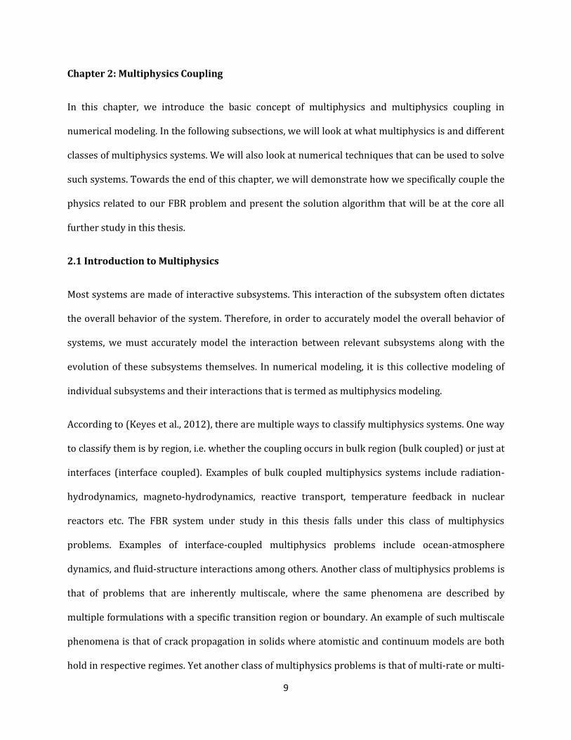
According to (Keyes et al., 2012), there are multiple ways to classify multiphysics systems. One way

to classify them is by region, i.e. whether the coupling occurs in bulk region (bulk coupled) or just at

interfaces (interface coupled). Examples of bulk coupled multiphysics systems include radiation-

hydrodynamics, magneto-hydrodynamics, reactive transport, temperature feedback in nuclear

reactors etc. The FBR system under study in this thesis falls under this class of multiphysics

problems. Examples of interface-coupled multiphysics problems include ocean-atmosphere

dynamics, and fluid-structure interactions among others. Another class of multiphysics problems is

that of problems that are inherently multiscale, where the same phenomena are described by

multiple formulations with a specific transition region or boundary. An example of such multiscale

phenomena is that of crack propagation in solids where atomistic and continuum models are both

hold in respective regimes. Yet another class of multiphysics problems is that of multi-rate or multi-

10

resolution problems. Other classes of multiphysics problems include systems of partial differential

equations that include equations of different types and the ones with different discretization for the

same physical model.

Figure 1: Multiphysics Classification

Each class of multiphysics problems, whether multiscale, multirate, multilevel, or multimodel,

include partitioning of the overall system into subparts or subsystems that evolve through a

sequence of updates of dependent variables (Keyes et al., 2012). More details on each class of the

multiphysics problems can be found in (Keyes et al. 2012). The evolution of these problems,

however, depends heavily on how the subsystems interact. That is discussed in the next subsection

on multiphysics coupling.

2.2 Introduction to Coupling

Coupling describes how the subsystems of the multiphysics systems interact. The coupling can be

classified into one-way coupled and two-way coupled problems depending on how subsystems

11

depend on each other. A one-way coupled system typically consists of a system of equations with

only forward or backward dependence. In other words, the system of equations is linearly coupled

and can be solved in a sequential manner. Two-way coupled systems consist of systems of

equations with both forward and backward dependence. These are non-linearly coupled systems

and require nonlinear iteration for their solution. Nonlinearly coupled systems may further be

classified into different classes depending on the solution strategy. The coupling may be tight or

loose. Loosely coupled systems typically arise out or a Gauss Seidel type or an operator split type

solution strategy. Picard iteration is predominantly used here. Tight coupling results from Newton

type solve (Keyes et al., 2012).

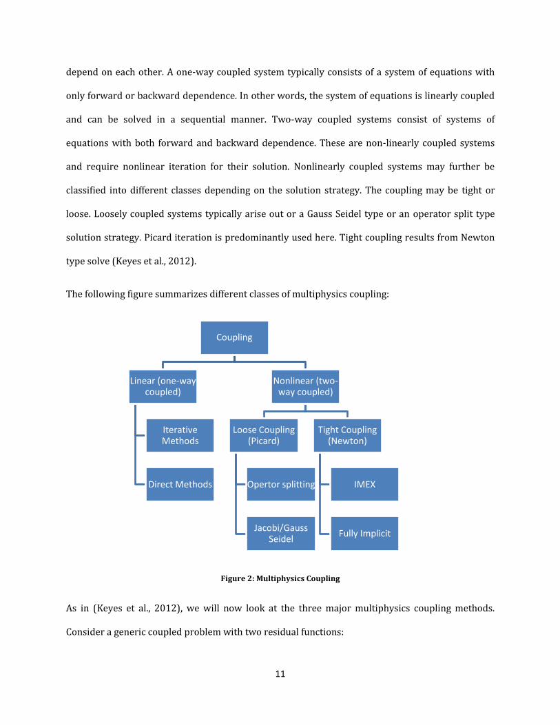
The following figure summarizes different classes of multiphysics coupling:

Figure 2: Multiphysics Coupling

As in (Keyes et al., 2012), we will now look at the three major multiphysics coupling methods.

Consider a generic coupled problem with two residual functions:

Coupling

Linear (one-way coupled)

Iterative Methods

Direct Methods

Nonlinear (two-way coupled)

Loose Coupling (Picard)

Opertor splitting

Jacobi/Gauss Seidel

Tight Coupling (Newton)

IMEX

Fully Implicit

12

(9)

(10)

In order to model the coupled system of Eq. (9) and Eq. (10), we may typically employ three

different strategies:

Gauss Seidel Method: This is the most widely used multiphysics coupling strategy. It preserves the

integrity of each subsystem where it solves respective subsystems separately, sequentially, and

then iterates until desired convergence is observed. The following algorithm describes this type of

coupling.

Gauss Seidel Coupling (Keyes et al., 2012):

1) Supply initial fields, and .

2) Start a while loop until convergence with iteration index g.

3) Compute in .

4) Set .

5) Compute in .

6) Set .

7) Loop back

8) Loop over to the next time step if the process is transient.

These types of algorithms result in loose coupling.

Operator Splitting: Time evolution problems often utilize operator splitting methods in time. The

following algorithm describes how a generic operator splitting method works.

Operator Split Coupling (Keyes et al., 2012):

13

1) Supply initial fields, and .

2) Start time loop with iteration index, t.

3) March in time with to compute .

4) March in time with to compute .

5) Loop back to the next time step.

Each individual time march in the above algorithm may be implicit or explicit. We may or may not

have within time-march iterations known as subcycling to obtain better quality solutions. We may

also stagger the solution in time. The above algorithm results in first order time splitting errors

which renders the solution first order accurate inspite of using higher order discretization schemes.

Higher order operator schemes like Strang splitting and temporal Richardson extrapolation must

be used to obtain higher order solution accuracy for the coupled system while using operator split

coupling technique (Keyes et al., 2012). This method of coupling also results in loose coupling.

Newton Method: As per (Keyes et al., 2012), this method takes into account all the subsystems of

the multiphysics model and formulates a single residual function. In other words,

[

] = 0. (11)

Let . The Jacobian of the equation system is given by

[

]

(12)

The following algorithm is used for Newton solve of the multiphysics system.

Newton’s Method (Keyes et al., 2012):

1) Supply initial field .

2) Start a while loop for convergence with iteration index, k.

14

3) Compute correction , using ( ) .

4) Update .

5) Loop back.

6) Loop back to the next time step for transient problems.

Newton’s method results in tight coupling. The Newton system in step 3 of the above algorithm can

be solved by multiple different methods (Kelley, 2003). We can employ direct methods or iterative

methods to solve that system. Sometimes, however, calculating the exact Jacobian becomes quite

tedious in which case, Jacobian Free Newton-Krylov (JFNK) method becomes very useful (Knoll et

al., 2002).

Now that we’ve seen the three basic coupling schemes, we move on to the next subsection where

we will describe the coupling scheme to be used for modeling the FBR problem. We will also discuss

Newton’s method in more detail.

2.3 FBR Coupling Scheme

The coupled FBR system can be solved iteratively using Newton’s method (Kelley, 2003). Newton’s

method iteratively finds the solution U that satisfies the relevant nonlinear residual functions,

. (13)

Here, F is the nonlinear residual function. In our FBR system, , and .

In order to solve Eq. 13, Newton’s method utilizes Taylor series expansion,

. (14)

Rearranging the above equation yields,

15

where,

(15)

(16)

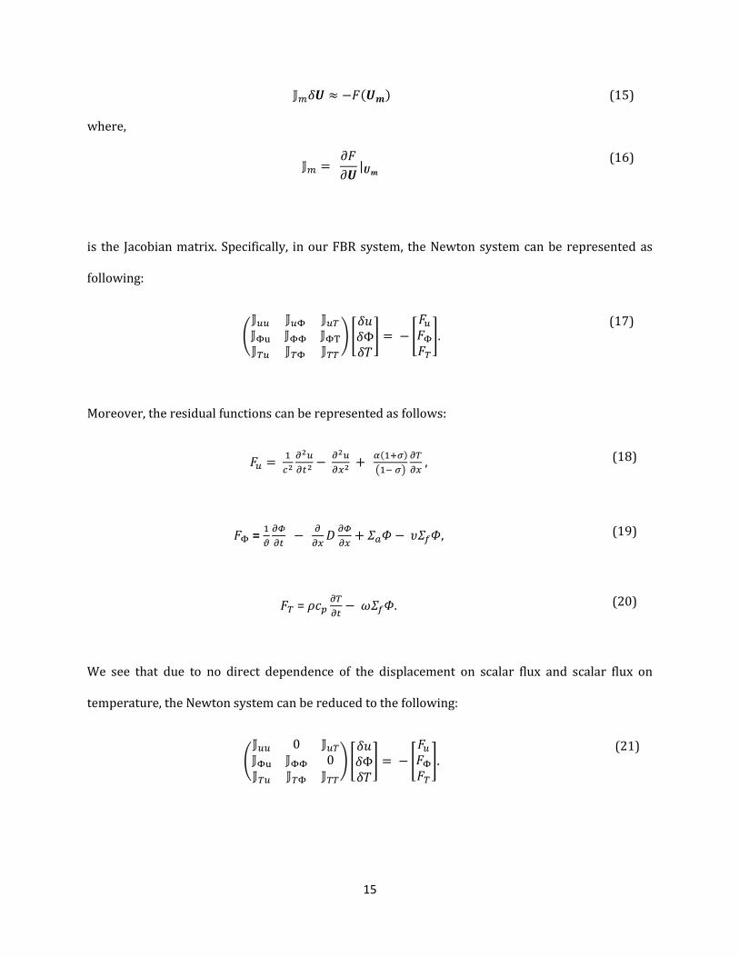
is the Jacobian matrix. Specifically, in our FBR system, the Newton system can be represented as

following:

(

) [

] [

]. (17)

Moreover, the residual functions can be represented as follows:

( )

,

(18)

=

,

(19)

=

.

(20)

We see that due to no direct dependence of the displacement on scalar flux and scalar flux on

temperature, the Newton system can be reduced to the following:

(

) [

] [

]. (21)

16

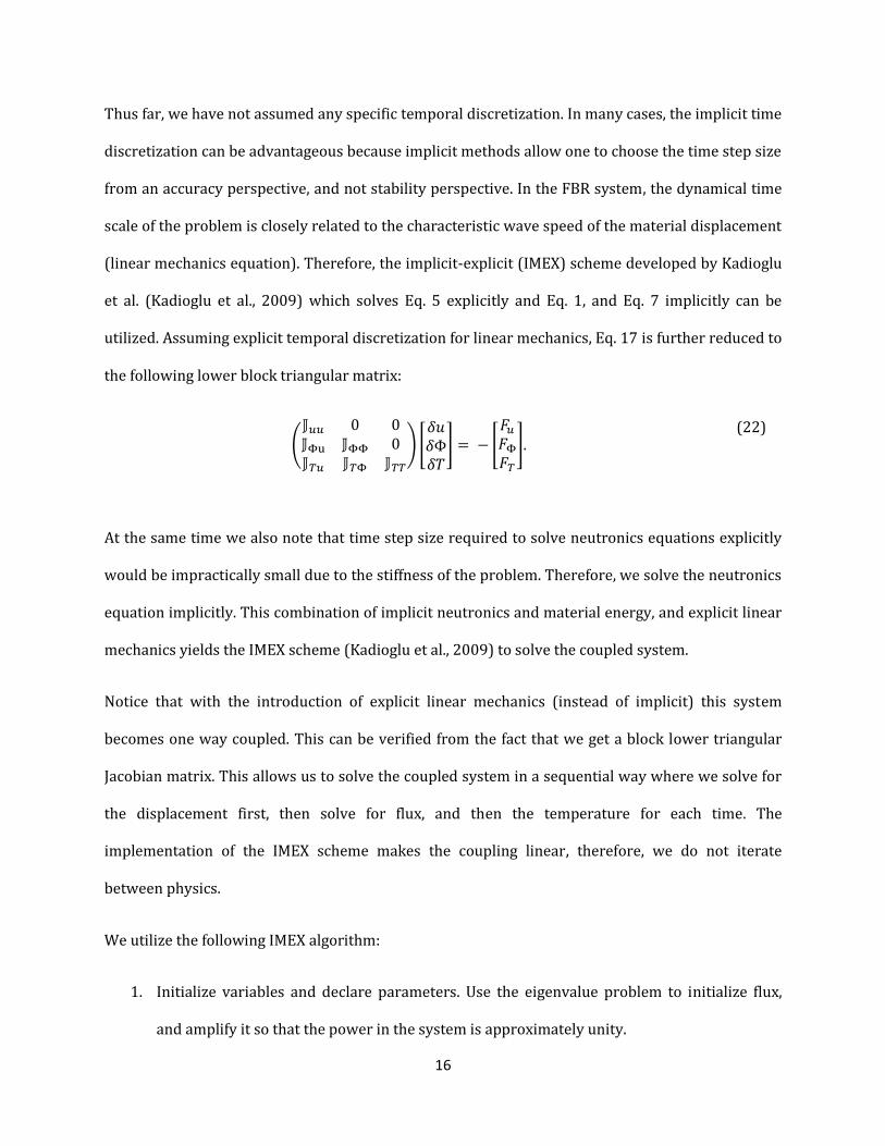
Thus far, we have not assumed any specific temporal discretization. In many cases, the implicit time

discretization can be advantageous because implicit methods allow one to choose the time step size

from an accuracy perspective, and not stability perspective. In the FBR system, the dynamical time

scale of the problem is closely related to the characteristic wave speed of the material displacement

(linear mechanics equation). Therefore, the implicit-explicit (IMEX) scheme developed by Kadioglu

et al. (Kadioglu et al., 2009) which solves Eq. 5 explicitly and Eq. 1, and Eq. 7 implicitly can be

utilized. Assuming explicit temporal discretization for linear mechanics, Eq. 17 is further reduced to

the following lower block triangular matrix:

(

) [

] [

]. (22)

At the same time we also note that time step size required to solve neutronics equations explicitly

would be impractically small due to the stiffness of the problem. Therefore, we solve the neutronics

equation implicitly. This combination of implicit neutronics and material energy, and explicit linear

mechanics yields the IMEX scheme (Kadioglu et al., 2009) to solve the coupled system.

Notice that with the introduction of explicit linear mechanics (instead of implicit) this system

becomes one way coupled. This can be verified from the fact that we get a block lower triangular

Jacobian matrix. This allows us to solve the coupled system in a sequential way where we solve for

the displacement first, then solve for flux, and then the temperature for each time. The

implementation of the IMEX scheme makes the coupling linear, therefore, we do not iterate

between physics.

We utilize the following IMEX algorithm:

1. Initialize variables and declare parameters. Use the eigenvalue problem to initialize flux,

and amplify it so that the power in the system is approximately unity.

17

2. March the explicit linear mechanics equation in time to calculate the displacement profile.

3. Calculate resultant density change and update density.

4. Update cross sections resulting from change in density.

5. March the implicit neutronics equation to calculate a new flux profile.

6. March the implicit temperature equation to calculate a new temperature profile

7. Loop back for next time step.

18

Chapter 3: Modeling the FBR System

In this chapter, we solve the FBR problem using diffusion, and transport (SN) neutronics. First, we

model the system with diffusion neutronics. Then we present the motivation for extension to

transport neutronics and compare the results from diffusion and transport neutronics.

3.1 Model System

Reactor System

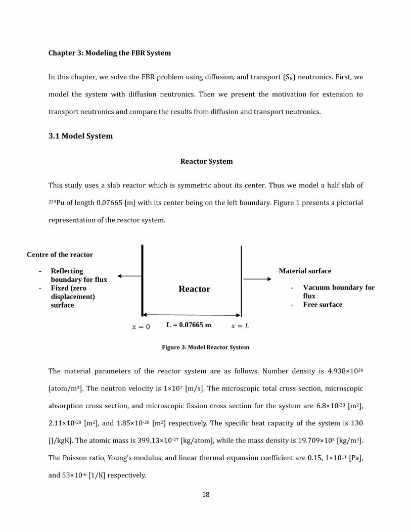
This study uses a slab reactor which is symmetric about its center. Thus we model a half slab of

239Pu of length 0.07665 [m] with its center being on the left boundary. Figure 1 presents a pictorial

representation of the reactor system.

Figure 3: Model Reactor System

The material parameters of the reactor system are as follows. Number density is 4.938×1028

[atom/m3]. The neutron velocity is 1×107 [m/s]. The microscopic total cross section, microscopic

absorption cross section, and microscopic fission cross section for the system are 6.8×10-28 [m2],

2.11×10-28 [m2], and 1.85×10-28 [m2] respectively. The specific heat capacity of the system is 130

[J/kgK]. The atomic mass is 399.13×10-27 [kg/atom], while the mass density is 19.709×103 [kg/m3].

The Poisson ratio, Young’s modulus, and linear thermal expansion coefficient are 0.15, 1×1011 [Pa],

and 53×10-6 [1/K] respectively.

L = 0.07665 m

Reactor

Material surface

- Vacuum boundary for

flux

- Free surface

Centre of the reactor

- Reflecting

boundary for flux

- Fixed (zero

displacement)

surface

𝑥 𝑥 𝐿

19

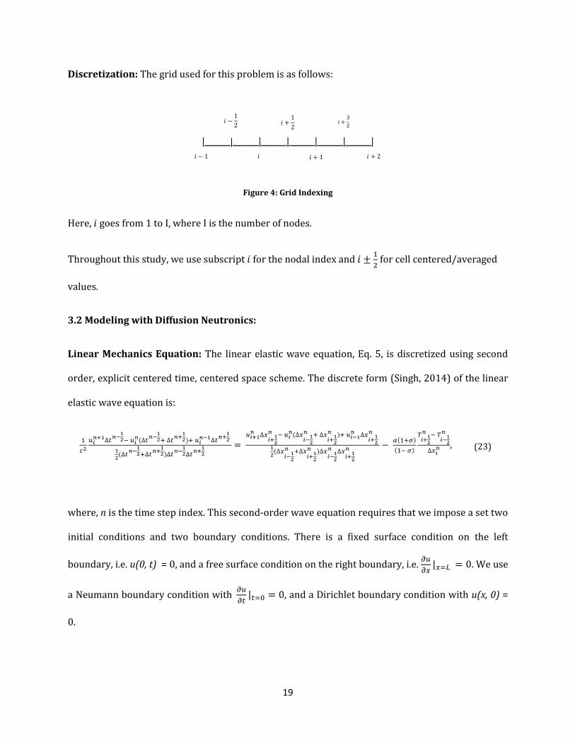
Discretization: The grid used for this problem is as follows:

|_____|_____|_____|_____|_____|_____|

Figure 4: Grid Indexing

Here, goes from 1 to I, where I is the number of nodes.

Throughout this study, we use subscript for the nodal index and

for cell centered/averaged

values.

3.2 Modeling with Diffusion Neutronics:

Linear Mechanics Equation: The linear elastic wave equation, Eq. 5, is discretized using second

order, explicit centered time, centered space scheme. The discrete form (Singh, 2014) of the linear

elastic wave equation is:

,

(23)

where, n is the time step index. This second-order wave equation requires that we impose a set two

initial conditions and two boundary conditions. There is a fixed surface condition on the left

boundary, i.e. u(0, t) = 0, and a free surface condition on the right boundary, i.e.

. We use

a Neumann boundary condition with

, and a Dirichlet boundary condition with u(x, 0) =

0.

𝑖

𝑖

𝑖 𝑖 𝑖 𝑖

𝑖 3

20

Neutron Diffusion Equation: The transient diffusion equation, Eq. 3, is discretized using the finite

volume method in space and implicit backward difference method in time. The discrete form of the

transient neutron diffusion equation is

.

(24)

There is a reflecting boundary condition on the left, i.e.

and a vacuum boundary

condition on the right, i.e. , where is the incoming partial current at

position L. To initialize neutronics, we run the eigenvalue problem. Then, we amplify the eigenflux

such that the system power is approximately unity. This amplified flux is used as the initial flux.

Adiabatic heat-up: The temperature equation, Eq. 7, is discretized in time using the implicit

backward difference formulation. The discretized form of the temperature equation is as follows:

. (25)

Since there is no spatial derivative, boundary conditions are not required. To initialize the

temperature, we set it to a uniform temperature field of 290K.

Simulation

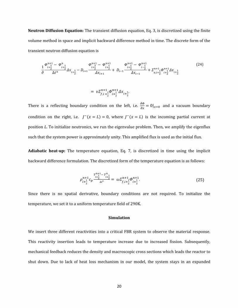
We insert three different reactivities into a critical FBR system to observe the material response.

This reactivity insertion leads to temperature increase due to increased fission. Subsequently,

mechanical feedback reduces the density and macroscopic cross sections which leads the reactor to

shut down. Due to lack of heat loss mechanism in our model, the system stays in an expanded

21

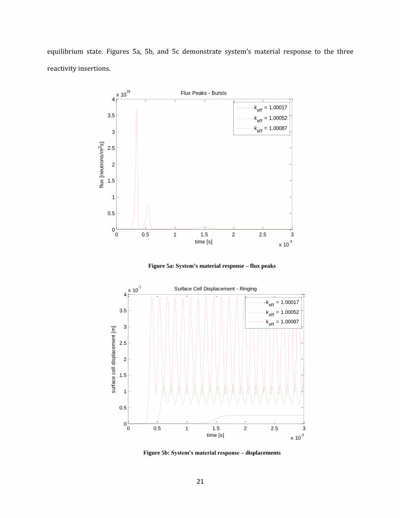
equilibrium state. Figures 5a, 5b, and 5c demonstrate system’s material response to the three

reactivity insertions.

Figure 5a: System’s material response – flux peaks

Figure 5b: System’s material response – displacements

0 0.5 1 1.5 2 2.5 3

x 10-3

0

0.5

1

1.5

2

2.5

3

3.5

4x 10

18 Flux Peaks - Bursts

time [s]

flux [

neutr

ons/m

2s]

keff

= 1.00017

keff

= 1.00052

keff

= 1.00087

0 0.5 1 1.5 2 2.5 3

x 10-3

0

0.5

1

1.5

2

2.5

3

3.5

4x 10

-7

surf

ace c

ell

dis

pla

cem

ent

[m]

time [s]

Surface Cell Displacement - Ringing

keff

= 1.00017

keff

= 1.00052

keff

= 1.00087

22

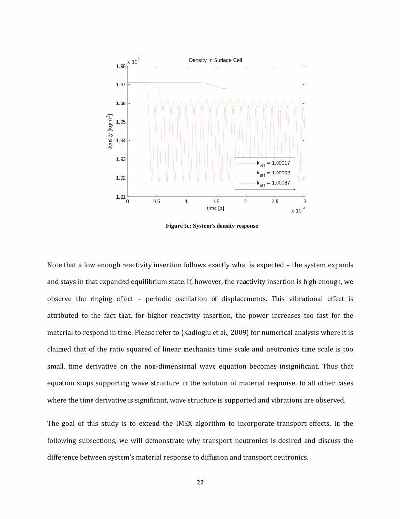
Figure 5c: System’s density response

Note that a low enough reactivity insertion follows exactly what is expected – the system expands

and stays in that expanded equilibrium state. If, however, the reactivity insertion is high enough, we

observe the ringing effect – periodic oscillation of displacements. This vibrational effect is

attributed to the fact that, for higher reactivity insertion, the power increases too fast for the

material to respond in time. Please refer to (Kadioglu et al., 2009) for numerical analysis where it is

claimed that of the ratio squared of linear mechanics time scale and neutronics time scale is too

small, time derivative on the non-dimensional wave equation becomes insignificant. Thus that

equation stops supporting wave structure in the solution of material response. In all other cases

where the time derivative is significant, wave structure is supported and vibrations are observed.

The goal of this study is to extend the IMEX algorithm to incorporate transport effects. In the

following subsections, we will demonstrate why transport neutronics is desired and discuss the

difference between system’s material response to diffusion and transport neutronics.

0 0.5 1 1.5 2 2.5 3

x 10-3

1.91

1.92

1.93

1.94

1.95

1.96

1.97

1.98x 10

4

time [s]

density [

kg/m

3]

Density in Surface Cell

keff

= 1.00017

keff

= 1.00052

keff

= 1.00087

23

3.3 Extension to Transport Neutronics

Why Extend to Transport Neutronics

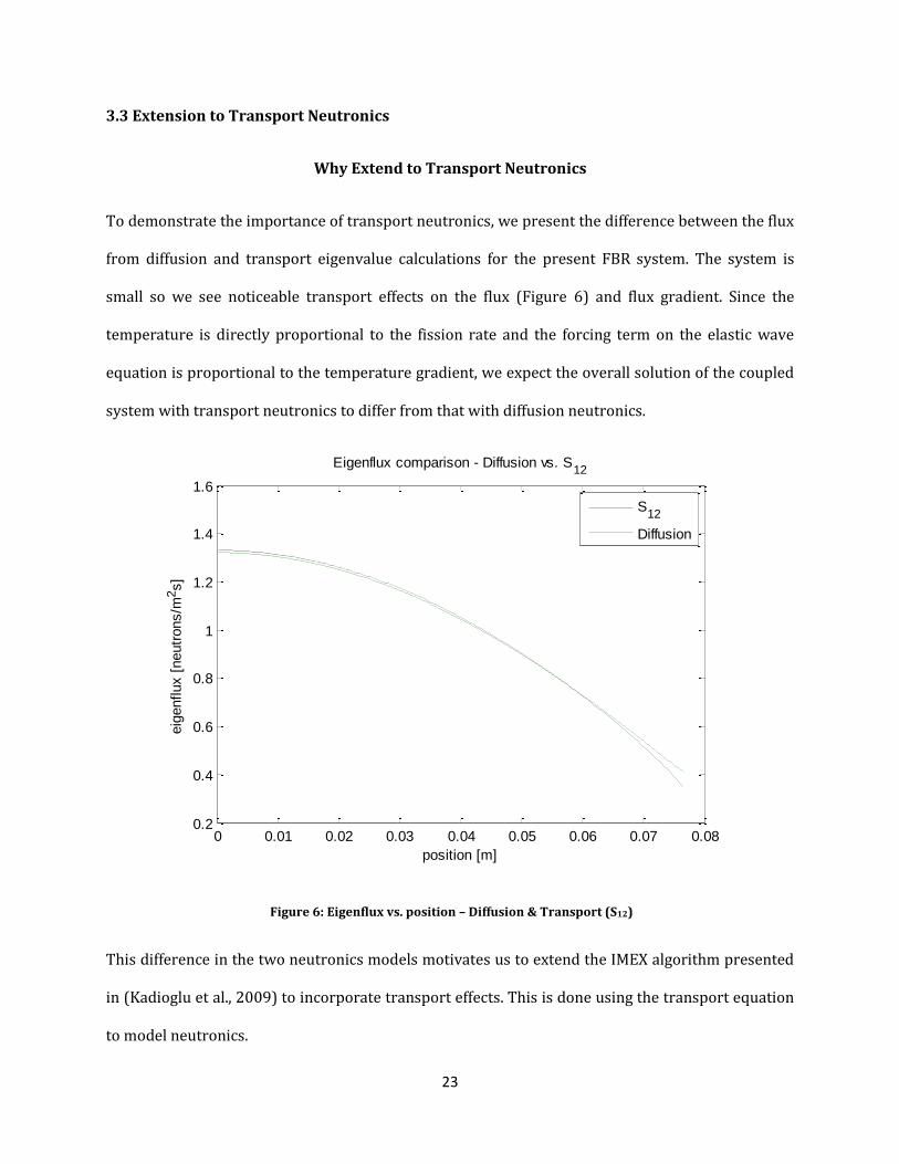
To demonstrate the importance of transport neutronics, we present the difference between the flux

from diffusion and transport eigenvalue calculations for the present FBR system. The system is

small so we see noticeable transport effects on the flux (Figure 6) and flux gradient. Since the

temperature is directly proportional to the fission rate and the forcing term on the elastic wave

equation is proportional to the temperature gradient, we expect the overall solution of the coupled

system with transport neutronics to differ from that with diffusion neutronics.

Figure 6: Eigenflux vs. position – Diffusion & Transport (S12)

This difference in the two neutronics models motivates us to extend the IMEX algorithm presented

in (Kadioglu et al., 2009) to incorporate transport effects. This is done using the transport equation

to model neutronics.

0 0.01 0.02 0.03 0.04 0.05 0.06 0.07 0.080.2

0.4

0.6

0.8

1

1.2

1.4

1.6

position [m]

eig

enflux [

neutr

ons/m

2s]

Eigenflux comparison - Diffusion vs. S12

S12

Diffusion

24

Discretization

The transient transport equation, Eq. 2, is discretized in space using diamond difference, and in

angle using the SN method. We use the one group approximation for treatment of energy, and we

assume isotropic scattering. We use Backward Euler (BDF-1) implicit time stepping. The following

equation represents the time discrete form of the transport equation:

.

(26)

Here, is the angular cosine index, is the iteration index, and is the mth angular cosine.

We have the same discrete forms of the wave equation and temperature equation as given by Eq. 23

and Eq. 25 respectively.

Coupling Scheme

In order to incorporate transport neutronics in our FBR model, we simply replace the diffusion

equation by the transport equation. As a result, we have the following Newton system:

(

) [

] *

+,

(27)

where, the residual function, , is as follows:

=

. (28)

Note that the system of Eq. 27 is still one-way coupled in physics, so we can solve it in a sequential

way.

25

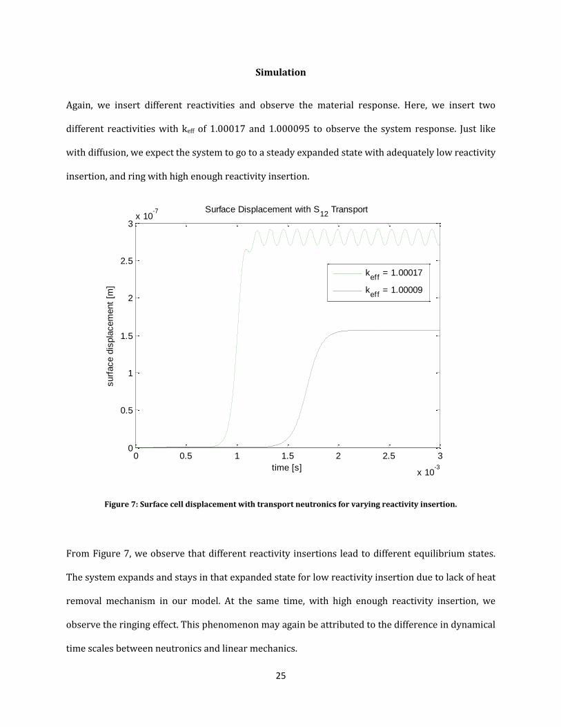
Simulation

Again, we insert different reactivities and observe the material response. Here, we insert two

different reactivities with keff of 1.00017 and 1.000095 to observe the system response. Just like

with diffusion, we expect the system to go to a steady expanded state with adequately low reactivity

insertion, and ring with high enough reactivity insertion.

Figure 7: Surface cell displacement with transport neutronics for varying reactivity insertion.

From Figure 7, we observe that different reactivity insertions lead to different equilibrium states.

The system expands and stays in that expanded state for low reactivity insertion due to lack of heat

removal mechanism in our model. At the same time, with high enough reactivity insertion, we

observe the ringing effect. This phenomenon may again be attributed to the difference in dynamical

time scales between neutronics and linear mechanics.

0 0.5 1 1.5 2 2.5 3

x 10-3

0

0.5

1

1.5

2

2.5

3x 10

-7

time [s]

surf

ace d

ispla

cem

ent

[m]

Surface Displacement with S12

Transport

keff

= 1.00017

keff

= 1.00009

26

In conclusion, we observe similar material behavior with transport as we observed with diffusion.

However, note the difference in keff used for transport and diffusion. This is a major discrepancy. In

the next subsection, we will present a detailed comparison between diffusion and transport models

with respect to FBR transient simulations.

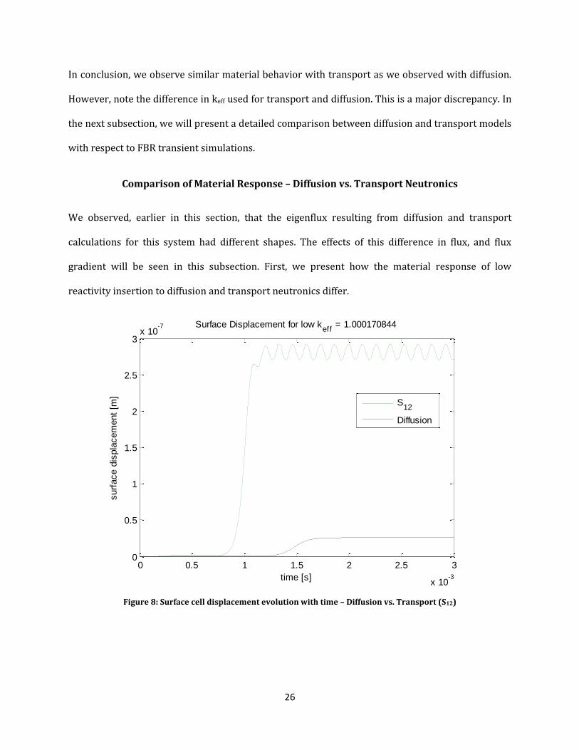
Comparison of Material Response – Diffusion vs. Transport Neutronics

We observed, earlier in this section, that the eigenflux resulting from diffusion and transport

calculations for this system had different shapes. The effects of this difference in flux, and flux

gradient will be seen in this subsection. First, we present how the material response of low

reactivity insertion to diffusion and transport neutronics differ.

Figure 8: Surface cell displacement evolution with time – Diffusion vs. Transport (S12)

0 0.5 1 1.5 2 2.5 3

x 10-3

0

0.5

1

1.5

2

2.5

3x 10

-7

time [s]

surf

ace d

ispla

cem

ent

[m]

Surface Displacement for low keff

= 1.000170844

S12

Diffusion

27

From Figure 8, we observe that for a small reactivity insertion, with keff of 1.00017, the system rings

with transport neutronics but the system goes to an expanded non vibrational state with diffusion

neutronics. This results from the difference in the dynamical time scales that diffusion and

transport neutronics exhibit. We note that flux evolution of the system with diffusion neutronics is

slow enough for the system to settle into a new equilibrium state after undergoing material

expansion. That, however, is not the case with transport neutronics where the material response

doesn’t keep up with the flux evolution in time. Therefore, we observe material ringing with

transport neutronics for this particular reactivity insertion.

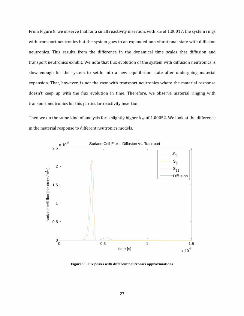
Then we do the same kind of analysis for a slightly higher keff of 1.00052. We look at the difference

in the material response to different neutronics models.

Figure 9: Flux peaks with different neutronics approximations

0 0.5 1 1.5

x 10-3

0

0.5

1

1.5

2

2.5x 10

19

time [s]

surf

ace c

ell

flux [

neutr

ons/m

2s]

Surface Cell Flux - Diffusion vs. Transport

S2

S6

S12

Diffusion

28

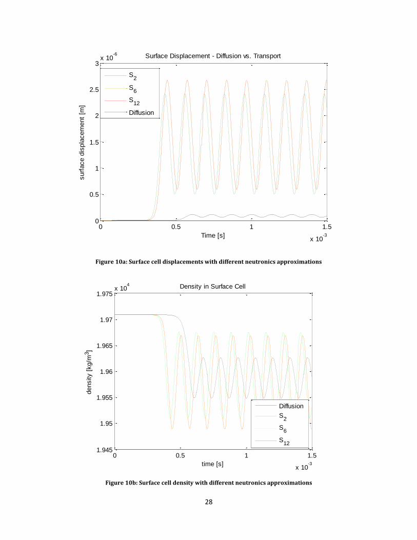
Figure 10a: Surface cell displacements with different neutronics approximations

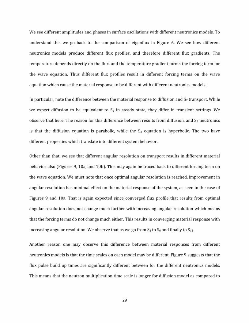
Figure 10b: Surface cell density with different neutronics approximations

0 0.5 1 1.5

x 10-3

0

0.5

1

1.5

2

2.5

3x 10

-6

Time [s]

surf

ace d

ispla

cem

ent

[m]

Surface Displacement - Diffusion vs. Transport

S2

S6

S12

Diffusion

0 0.5 1 1.5

x 10-3

1.945

1.95

1.955

1.96

1.965

1.97

1.975x 10

4

time [s]

density [

kg/m

3]

Density in Surface Cell

Diffusion

S2

S6

S12

29

We see different amplitudes and phases in surface oscillations with different neutronics models. To

understand this we go back to the comparison of eigenflux in Figure 6. We see how different

neutronics models produce different flux profiles, and therefore different flux gradients. The

temperature depends directly on the flux, and the temperature gradient forms the forcing term for

the wave equation. Thus different flux profiles result in different forcing terms on the wave

equation which cause the material response to be different with different neutronics models.

In particular, note the difference between the material response to diffusion and S2 transport. While

we expect diffusion to be equivalent to S2 in steady state, they differ in transient settings. We

observe that here. The reason for this difference between results from diffusion, and S2 neutronics

is that the diffusion equation is parabolic, while the S2 equation is hyperbolic. The two have

different properties which translate into different system behavior.

Other than that, we see that different angular resolution on transport results in different material

behavior also (Figures 9, 10a, and 10b). This may again be traced back to different forcing term on

the wave equation. We must note that once optimal angular resolution is reached, improvement in

angular resolution has minimal effect on the material response of the system, as seen in the case of

Figures 9 and 10a. That is again expected since converged flux profile that results from optimal

angular resolution does not change much further with increasing angular resolution which means

that the forcing terms do not change much either. This results in converging material response with

increasing angular resolution. We observe that as we go from S2 to S6 and finally to S12.

Another reason one may observe this difference between material responses from different

neutronics models is that the time scales on each model may be different. Figure 9 suggests that the

flux pulse build up times are significantly different between for the different neutronics models.

This means that the neutron multiplication time scale is longer for diffusion model as compared to

30

the transport model. This is expected since the diffusion model exhibits more neutron leakage and

higher scattering.

Now, we note that source iteration is not necessarily the best way to solve the transport equation.

We also note the benefit in isolating the angular flux from the coupled system, especially while we

are dealing with a more complicated 3D system or a fully coupled nonlinear system, while retaining

the transport effects. This can be done by introducing the moment based acceleration – scale

bridging HOLO concept – into the neutronics model. We will discuss this concept in the next section.

31

Chapter 4: Extension to Moment Based Acceleration

In this section, we extend the IMEX scheme to incorporate moment-based acceleration (Smith et al.,

2002), (Knoll et al., 2011), (Park et al., 2012) for neutronics into the coupled system. One of its main

advantages, as the name suggests, is that it accelerates slowly converging physics like fission

and/or scattering source. This reduces the number of iterations required per time-step to get the

new scalar flux. This fact is widely known. The other advantage is that it allows us to isolate the

angular flux from the coupled system by introducing a discretely consistent LO system which

resembles the diffusion equation. This moment based acceleration concept is a scale bridging

concept because it essentially bridges transport and diffusion equations with distinct

corresponding length scales using the drift term in the LO equation.

4.1 Standard SN vs. Nonlinear Diffusion Accelerated SN (Moment-Based Acceleration)

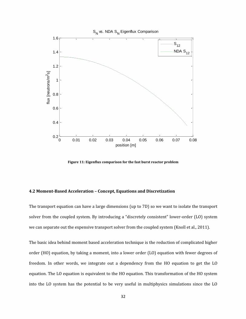
Here, we show consistency of the accelerated transport solution to the eigenvalue problem for the

present fast burst system. The problem parameters have been stated in section 4.1. Figure 11

shows a comparison between the standard SN solution and the accelerated SN solution. We observe

that the nonlinear diffusion accelerated SN follows the standard SN solution quite closely. The

relative error norm was found to be 1.7043×10-9.

The total number of transport sweeps required with standard SN was 156, while the total number

required with HOLO (NDA SN) iteration was 19. Clearly, if we were to solve a transient coupled

problem, which could involve several hundred thousand time-steps, then using accelerated SN

instead of standard SN with source iteration would be a good idea. Therefore this is one reason why

we proceed to extend the present IMEX algorithm to incorporate moment-based acceleration

concept. The other reason will be explained in the next subsection.

32

Figure 11: Eigenflux comparison for the fast burst reactor problem

4.2 Moment-Based Acceleration – Concept, Equations and Discretization

The transport equation can have a large dimensions (up to 7D) so we want to isolate the transport

solver from the coupled system. By introducing a “discretely consistent” lower-order (LO) system

we can separate out the expensive transport solver from the coupled system (Knoll et al., 2011).

The basic idea behind moment based acceleration technique is the reduction of complicated higher

order (HO) equation, by taking a moment, into a lower order (LO) equation with fewer degrees of

freedom. In other words, we integrate out a dependency from the HO equation to get the LO

equation. The LO equation is equivalent to the HO equation. This transformation of the HO system

into the LO system has the potential to be very useful in multiphysics simulations since the LO

0 0.01 0.02 0.03 0.04 0.05 0.06 0.07 0.080.2

0.4

0.6

0.8

1

1.2

1.4

1.6

position [m]

flux [

neutr

ons/m

2s]

SN vs. NDA S

N Eigenflux Comparison

S12

NDA S12

33

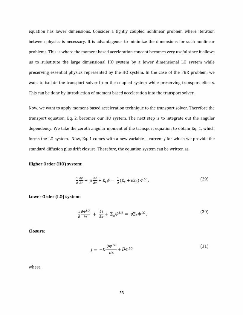
equation has lower dimensions. Consider a tightly coupled nonlinear problem where iteration

between physics is necessary. It is advantageous to minimize the dimensions for such nonlinear

problems. This is where the moment based acceleration concept becomes very useful since it allows

us to substitute the large dimensional HO system by a lower dimensional LO system while

preserving essential physics represented by the HO system. In the case of the FBR problem, we

want to isolate the transport solver from the coupled system while preserving transport effects.

This can be done by introduction of moment based acceleration into the transport solver.

Now, we want to apply moment-based acceleration technique to the transport solver. Therefore the

transport equation, Eq. 2, becomes our HO system. The next step is to integrate out the angular

dependency. We take the zeroth angular moment of the transport equation to obtain Eq. 1, which

forms the LO system. Now, Eq. 1 comes with a new variable – current J for which we provide the

standard diffusion plus drift closure. Therefore, the equation system can be written as,

Higher Order (HO) system:

, (29)

Lower Order (LO) system:

, (30)

Closure:

where,

(31)

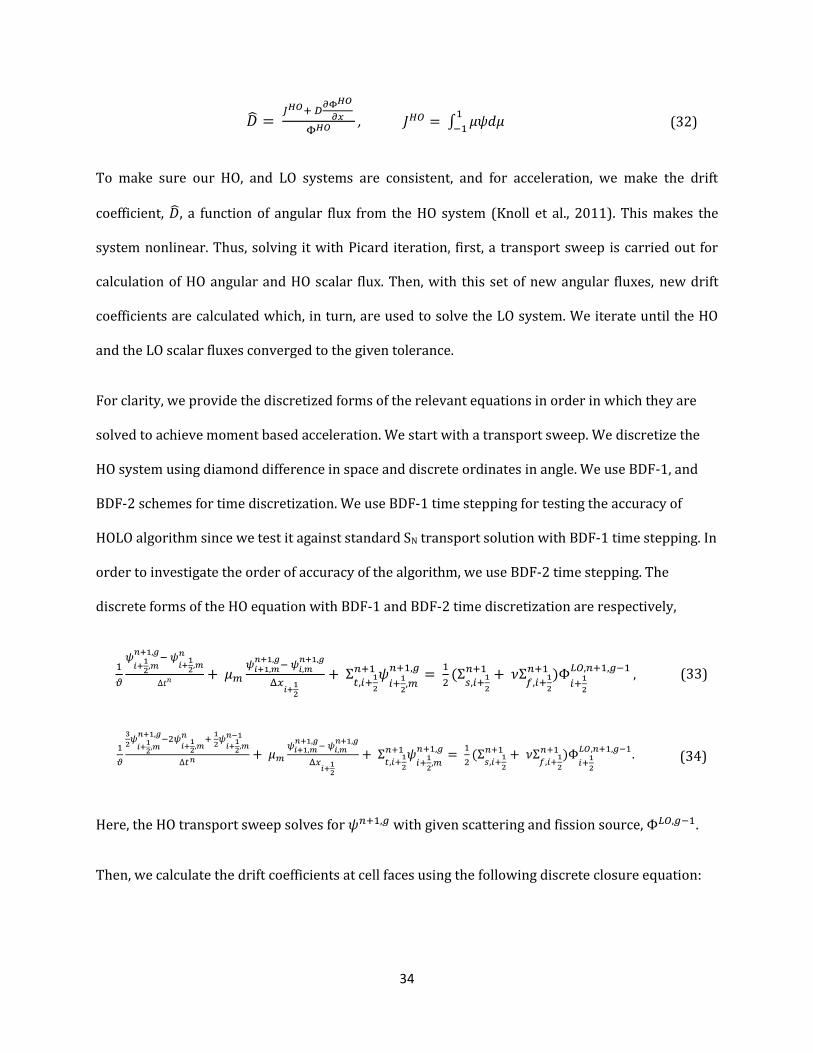
34

, ∫

(32)

To make sure our HO, and LO systems are consistent, and for acceleration, we make the drift

coefficient, , a function of angular flux from the HO system (Knoll et al., 2011). This makes the

system nonlinear. Thus, solving it with Picard iteration, first, a transport sweep is carried out for

calculation of HO angular and HO scalar flux. Then, with this set of new angular fluxes, new drift

coefficients are calculated which, in turn, are used to solve the LO system. We iterate until the HO

and the LO scalar fluxes converged to the given tolerance.

For clarity, we provide the discretized forms of the relevant equations in order in which they are

solved to achieve moment based acceleration. We start with a transport sweep. We discretize the

HO system using diamond difference in space and discrete ordinates in angle. We use BDF-1, and

BDF-2 schemes for time discretization. We use BDF-1 time stepping for testing the accuracy of

HOLO algorithm since we test it against standard SN transport solution with BDF-1 time stepping. In

order to investigate the order of accuracy of the algorithm, we use BDF-2 time stepping. The

discrete forms of the HO equation with BDF-1 and BDF-2 time discretization are respectively,

,

(33)

.

(34)

Here, the HO transport sweep solves for with given scattering and fission source, .

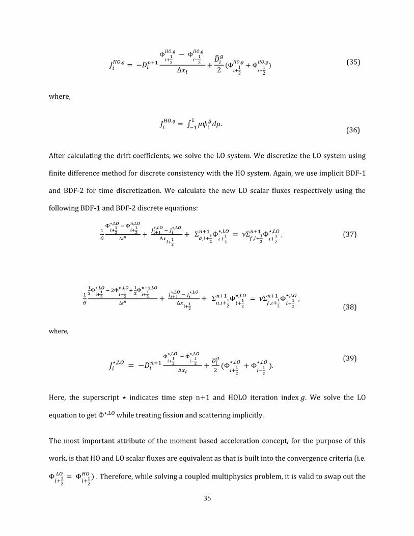
Then, we calculate the drift coefficients at cell faces using the following discrete closure equation:

35

where,

∫

.

(35)

(36)

After calculating the drift coefficients, we solve the LO system. We discretize the LO system using

finite difference method for discrete consistency with the HO system. Again, we use implicit BDF-1

and BDF-2 for time discretization. We calculate the new LO scalar fluxes respectively using the

following BDF-1 and BDF-2 discrete equations:

,

(37)

,

where,

.

(38)

(39)

Here, the superscript indicates time step n and HOLO iteration index . We solve the LO

equation to get while treating fission and scattering implicitly.

The most important attribute of the moment based acceleration concept, for the purpose of this

work, is that HO and LO scalar fluxes are equivalent as that is built into the convergence criteria (i.e.

. Therefore, while solving a coupled multiphysics problem, it is valid to swap out the

36

angular flux dependent transport (equivalent to purely HO system) solver for the diffusion equation

like diffusion plus drift LO system without affecting the solution of the problem (as long as the

transport problem is solved within the HOLO framework).

4.3 Coupling Scheme

Next, we incorporate the moment based acceleration method into our IMEX algorithm. We begin by

replacing the transport equation, in Eq. 27, with the LO equation. We get the following Newton step:

(

) [

] [

].

(40)

The residual function is given by,

=

. (41)

Note that we still have a one way coupled system which may be solved sequentially.

One may not necessarily see merit in replacing the angular flux for LO scalar flux in this particular

problem because of the one way coupling – we could couple the HO transport equation directly for

the multiphysics system (not isolating the angular variable) and the problem would still essentially

stay the same as long as we did our neutronics using a moment based acceleration technique. But

imagine a two way coupled problem, as stated before, where iteration between physics is necessary

- that is where this kind of substitution of equations can be really useful.

Another advantage of using the LO flux in the coupled system is the ease with which we can

transition from diffusion to transport as the LO system resembles the diffusion equation. All we

37

need to do is add a consistency term to the existing diffusion solver (plus a transport sweep for

calculation of the consistency term - outside the coupled system).

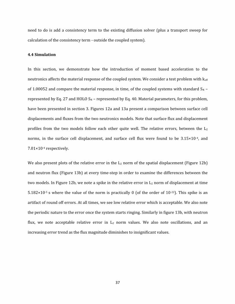
4.4 Simulation

In this section, we demonstrate how the introduction of moment based acceleration to the

neutronics affects the material response of the coupled system. We consider a test problem with keff

of 1.00052 and compare the material response, in time, of the coupled systems with standard SN –

represented by Eq. 27 and HOLO SN – represented by Eq. 40. Material parameters, for this problem,

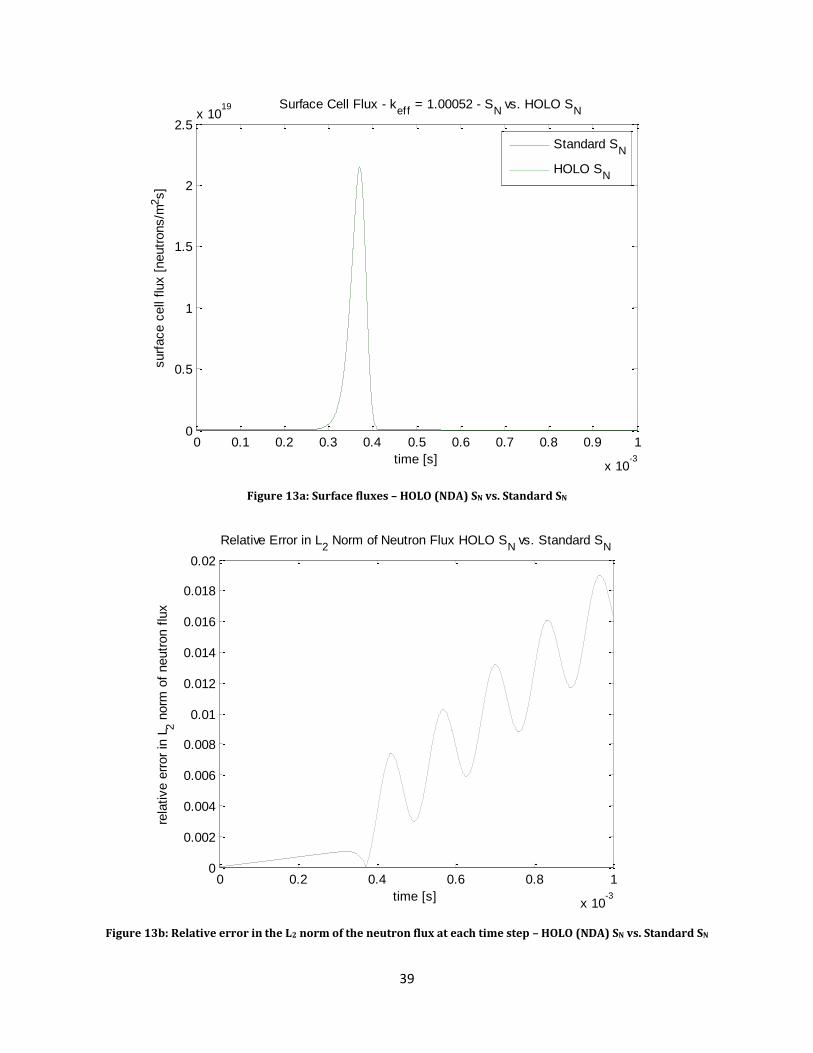
have been presented in section 3. Figures 12a and 13a present a comparison between surface cell

displacements and fluxes from the two neutronics models. Note that surface flux and displacement

profiles from the two models follow each other quite well. The relative errors, between the L2

norms, in the surface cell displacement, and surface cell flux were found to be 3.15×10-4, and

7.01×10-4 respectively.

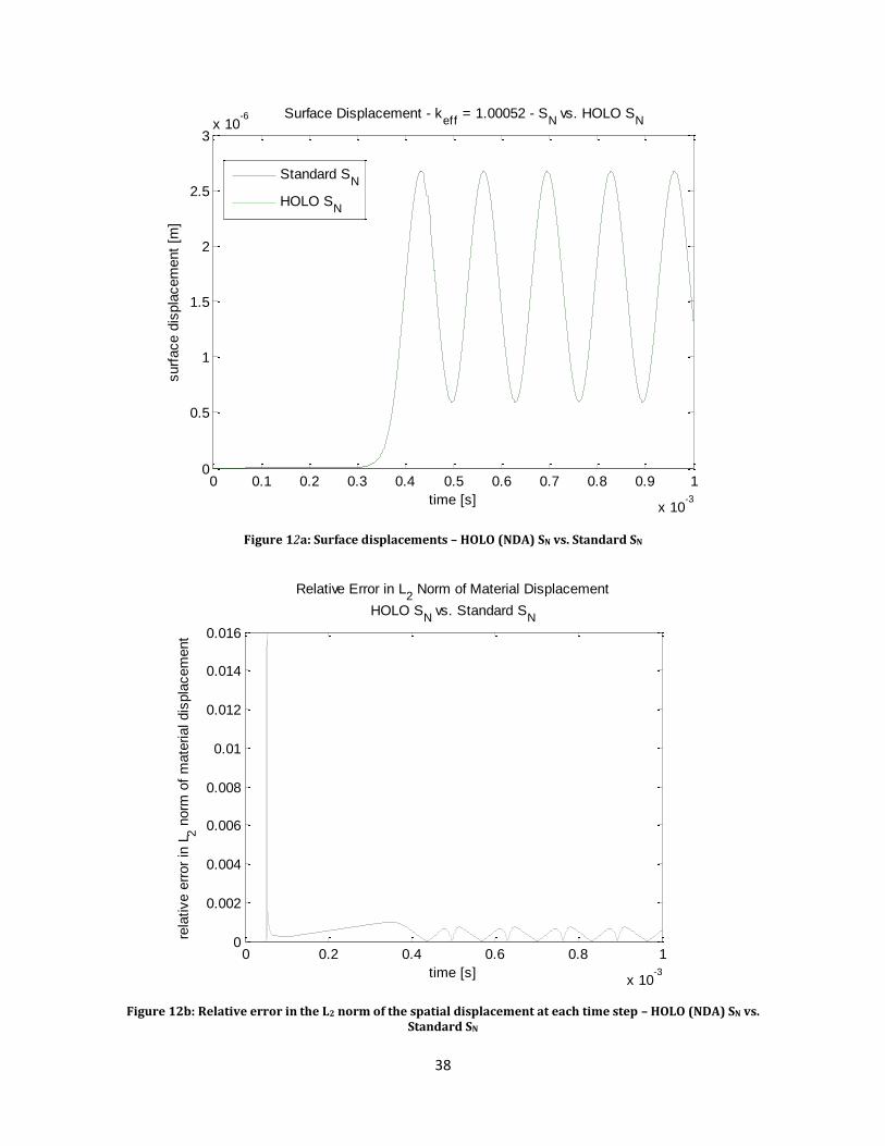
We also present plots of the relative error in the L2 norm of the spatial displacement (Figure 12b)

and neutron flux (Figure 13b) at every time-step in order to examine the differences between the

two models. In Figure 12b, we note a spike in the relative error in L2 norm of displacement at time

5.182×10-5 s where the value of the norm is practically 0 (of the order of 10-22). This spike is an

artifact of round off errors. At all times, we see low relative error which is acceptable. We also note

the periodic nature to the error once the system starts ringing. Similarly in figure 13b, with neutron

flux, we note acceptable relative error in L2 norm values. We also note oscillations, and an

increasing error trend as the flux magnitude diminishes to insignificant values.

38

Figure 12a: Surface displacements – HOLO (NDA) SN vs. Standard SN

Figure 12b: Relative error in the L2 norm of the spatial displacement at each time step – HOLO (NDA) SN vs. Standard SN

0 0.1 0.2 0.3 0.4 0.5 0.6 0.7 0.8 0.9 1

x 10-3

0

0.5

1

1.5

2

2.5

3x 10

-6

time [s]

surf

ace d

ispla

cem

ent

[m]

Surface Displacement - keff

= 1.00052 - SN vs. HOLO S

N

Standard SN

HOLO SN

0 0.2 0.4 0.6 0.8 1

x 10-3

0

0.002

0.004

0.006

0.008

0.01

0.012

0.014

0.016

time [s]

rela

tive e

rror

in L

2 n

orm

of

mate

rial dis

pla

cem

ent

Relative Error in L2 Norm of Material Displacement

HOLO SN vs. Standard S

N

39

Figure 13a: Surface fluxes – HOLO (NDA) SN vs. Standard SN

Figure 13b: Relative error in the L2 norm of the neutron flux at each time step – HOLO (NDA) SN vs. Standard SN

0 0.1 0.2 0.3 0.4 0.5 0.6 0.7 0.8 0.9 1

x 10-3

0

0.5

1

1.5

2

2.5x 10

19

time [s]

surf

ace c

ell

flux [

neutr

ons/m

2s]

Surface Cell Flux - keff

= 1.00052 - SN vs. HOLO S

N

Standard SN

HOLO SN

0 0.2 0.4 0.6 0.8 1

x 10-3

0

0.002

0.004

0.006

0.008

0.01

0.012

0.014

0.016

0.018

0.02

time [s]

rela

tive e

rror

in L

2 n

orm

of

neutr

on f

lux

Relative Error in L2 Norm of Neutron Flux HOLO S

N vs. Standard S

N

40

The plots examined in this subsection, along with satisfactory error norm numbers, prove the

applicability of the HOLO concept in true (although simplified) multiphysics setting.

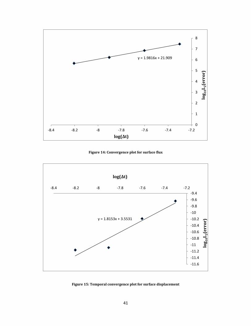
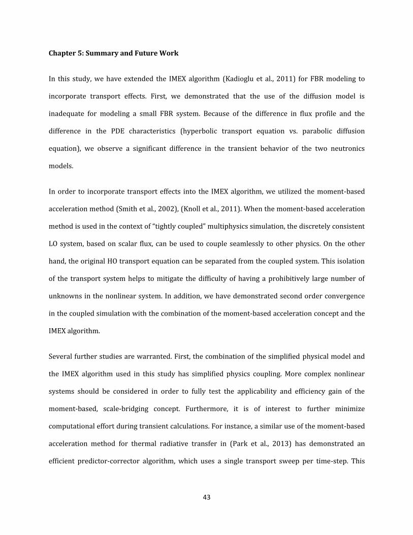
4.5 Convergence Study

Now, we look at the convergence rate for scalar flux, material displacement in order to determine

the quality of the coupled solution with HOLO transport neutronics, and IMEX coupling. To do that,

we use implicit BDF-2 time integration scheme for neutronics, and the temperature equations. Then

we run the transient coupled problem with five distinct time steps ranging from 1×10-7 to 6.25×10-9

s, for 0.5 ms time. We choose the total number of time steps, accordingly, for each time step size.

Table 1, along with figure 14 and figure 15, presents the data collected after running the five

transient simulations for this convergence study.

Time step

( )

Log( ) Log(||flux( ) –

flux( )||)

Log(||u( ) – u( )||)

5×10-8 -7.301029995663981 7.447863755282549 -9.641079015622641

2.5×10-8 -7.602059991327963 6.847704077101912 -10.189050265316403

1.25×10-8 -7.903089986991944 6.217734674605953 -11.088037041790605

6.25×10-9 -8.204119982655925 5.669407487493253 -11.162963763319620

Table 1: Convergence Data

41

Figure 14: Convergence plot for surface flux

Figure 15: Temporal convergence plot for surface displacement

y = 1.9816x + 21.909

0

1

2

3

4

5

6

7

8

-8.4 -8.2 -8 -7.8 -7.6 -7.4 -7.2

log

10L

2(e

rro

r)

log(Δt)

y = 1.8153x + 3.5531

-11.6

-11.4

-11.2

-11

-10.8

-10.6

-10.4

-10.2

-10

-9.8

-9.6

-9.4

-8.4 -8.2 -8 -7.8 -7.6 -7.4 -7.2

log

10L

2(e

rro

r)

log(Δt)

42

From table 1, figure 14, and figure 15, it is clear that we observe a convergence order of 1.98 for the

neutron flux, and of 1.82 for the displacement. Thus we get near second order convergence.

43

Chapter 5: Summary and Future Work

In this study, we have extended the IMEX algorithm (Kadioglu et al., 2011) for FBR modeling to

incorporate transport effects. First, we demonstrated that the use of the diffusion model is

inadequate for modeling a small FBR system. Because of the difference in flux profile and the

difference in the PDE characteristics (hyperbolic transport equation vs. parabolic diffusion

equation), we observe a significant difference in the transient behavior of the two neutronics

models.

In order to incorporate transport effects into the IMEX algorithm, we utilized the moment-based

acceleration method (Smith et al., 2002), (Knoll et al., 2011). When the moment-based acceleration

method is used in the context of “tightly coupled” multiphysics simulation, the discretely consistent

LO system, based on scalar flux, can be used to couple seamlessly to other physics. On the other

hand, the original HO transport equation can be separated from the coupled system. This isolation

of the transport system helps to mitigate the difficulty of having a prohibitively large number of

unknowns in the nonlinear system. In addition, we have demonstrated second order convergence

in the coupled simulation with the combination of the moment-based acceleration concept and the

IMEX algorithm.

Several further studies are warranted. First, the combination of the simplified physical model and

the IMEX algorithm used in this study has simplified physics coupling. More complex nonlinear

systems should be considered in order to fully test the applicability and efficiency gain of the

moment-based, scale-bridging concept. Furthermore, it is of interest to further minimize

computational effort during transient calculations. For instance, a similar use of the moment-based

acceleration method for thermal radiative transfer in (Park et al., 2013) has demonstrated an

efficient predictor-corrector algorithm, which uses a single transport sweep per time-step. This

44

kind of more sophisticated time-stepping may be desired when we extend the study to larger

multiphysics, multidimensional problems.

45

References

[1] E. Shabalin. Fast Pulsed and Burst Reactors. Pergamon Press (1979).

[2] D. Burgreen, Thermoelastic Dynamics of Rods, Thin Shells, and Solid Spheres. Nuclear Science

and Engineering: 12, 203 – 217 (1962).

[3] S. Kadioglu, D. Knoll, and C. de Oliveira, “Multi-physics Analysis of Spherical Fast Burst

Reactors”, Nuclear Science and Engineering: 163, 1-12, March 2009.

[4] M. L. Adams and E. W. Larsen, “Fast Iterative Methods for Discrete-Ordinates Particle Transport

Calculations,” Progress in Nuclear Energy, 40, No. 1, 3-159 (2002).

[5] Kopp H. J. (1963), “Synthetic Method Solution of the Transport Equation,” Nuclear Science and

Engineering, 17, 65.

[6] Lebedev V. I. (1967), “An Iterative KP Method,” USSR Comp. Math and Math. Phys. 7, 1250.

[7] Marchuk G. I. and Levedev (1986) Numerical Methods in Theory of Neutron Transport, Second

Revised Edition, Harwood Academic Publishers, London.

[8] Lebedev V. I. (1964), “The Iterative KP Method for the Kinetic Equation,” Proc. Conf on

Mathematical Methods for Solution of Nuclear Physics Problems, Nov. 17-20, 1964, Dubna, 93.

[9] Gelbard E. M. and Hageman L. A. (1969) “Convergence of Some Approximate Methods for

Solving the Transport Equation,” Nucl. Sci. Eng. 37, 288.

[10] Reed W. H. (1971) “The Effectiveness of Acceleration Techniques for Iterative Methods in

Transport Theory,” Nucl. Sci. Eng. 45, 245.

46

[11] Alcouffe R. E. (1976) “A Stable Diffusion Synthetic Acceleration Method for Neutron Transport

Iterations,” Nucl. Sci. Eng. 45, 245.

[12] Gol’din V. Ya. (1967) “Quasi-Diffusion Method for Solving the Transport Equation,” USSR Comp.

Math. and Math. Phys. 4, 136.

[13] Anistratov D. Y. and Larsen E. W. (1996) “Weighted Alpha Acceleration Methods for the

Transport Equation,” Trans. Am. Nucl. Soc. 75, 154.

[14] Larsen E. W. (1990) “Transport Acceleration Methods and Two Level Multigrid Algorithms”

Modern Mathematical Methods in Transport Theory (Operator Theory: Advances and Applications, Vol

51), W. Greenberg and J Polewczak, eds, Birkhauser Verlag, Basel, 34.

[15] Nowak P. F., Larsen E. W., and Martin W. R. (1987) “Multigrid Methods for SN Problems,” Trans.

Am. Nucl. Soc. 55, 355.

[16] Nowak P. F., Larsen E. W., and Martin W. R. (1988) “Multigrid Methods for SN Calculations in X-

Y Geometry,” Trans. Am. Nucl. Soc. 56, 291.

[17] Barnett A., Morel J. E., Harris D. R. (1989) “A Multigrid Acceleration for 1-D SN Equations with

Anisotropic Scattering,” Nucl. Sci. Eng., 102, 1.

[18] Ramone G. L., Larsen E. W., and Martin W. R. (1997) “ A Synthetic Acceleration Method for

Transport Iterations,” Nucl. Sci. Eng., 125, 257.

[19] Lewis E. E. and Miller W. F. Jr. (1976) “A comparison of P1 Synthetic Acceleration Techniques,”

Trans. Am. Nucl. Soc. 23, 202.

[20] Smith K. S. and Rhodes J. D. III (2000) “Casmo-4 Characteristics Methods for Two Dimensional

PWR and BWR Core Calculations,” Trans. Am. Nucl. Soc. 83, 294.

47

[21] Seker V., Thomas J. W., Downer T. J. (2007) “Reactor Simulation with Coupled Monte Carlo and

Computational Fluid Dynamics,” Joint International Topical Meeting on Mathematics & Computation

and Supercomputing in Nuclear Applications Am. Nucl. Soc., Monterey.

[22] Procasini R., Chand K., Clouse C., Ferencz R., Grandy J., Henshaw W., Kramer K., Parsons D.

(2007) “OSIRIS: A Modern, High Performance, Coupled, Multiphysics Code for Nuclear Reactor Core

Analysis,” Joint International Topical Meeting on Mathematics & Computation and Supercomputing in

Nuclear Applications Am. Nucl. Soc., Monterey.

[23] Lockwood B. A. (2007) “A Two Dimensional Fluid Dynamics Solver for Use in Multiphysics

Simulation of Gas Cooled Reactors,” PhD. Dissertation, Georgia Institute of Technology, Atlanta.

[24] McTaggart M. H. (1969) “Fast Burst Reactor Kinetics,” Proceedings of National Topical Meeting

on Fast Burst Reactors, Albuquerque.

[25] Reuscher J. A. (1969) “Thermomechanical Analysis of Fast Burst Reactors,” Proceedings of

National Topical Meeting on Fast Burst Reactors, Albuquerque.

[26] Hetrick D. L., Kimpland R. H., and Kornreich D. E. (1994) “Computer Simulations of

Homogeneous Water Solution Pulse Reactors and Criticality Accidents,” Proceedings of National

Topical Meeting on Physics, Safety and Applications of Pulsed Reactors, Washington D. C.

[27] Pasternoster R., Kimpland R. H., Jaegers P., and McGhee J. (1994) “Coupled Hydro-Neutronic

Calculations for Fast Burst Reactor Analysis,” Proceedings of National Topical Meeting on Physics,

Safety and Applications of Pulsed Reactors, Washington D. C.

[28] Wilson S. C., Beigalski S. R., and Coats R. L. (2007) “Computational Modeling of Coupled

Thermomechanical and Neutron Transport Behavior in Godiva like Nuclear Assemblies,” Nucl. Sci.

Eng. 157, 344.

48

[29] Green T. C. (2008) “Simulation of Reactor Pulses in Fast Burst and Externally Driven

Assembliesm,” PhD Dissertation, University of Texas, Austin.

[30] Tamang, A, and Anistratov, D. (2013) “A Multilevel Method for Coupling the Neutron Kinetics

and Heat Transfer Equation,” SIAM Journal of Scientific Computations, 19, 266.

[31] Williamson, R. L., Hales, J. D, Novascone, S.R., Tonks, M. R., Gaston, D. R. Permann, C. J., Andrs,

D., and Martineau, R. C. (2012) “Multidimensional Multiphysics Simulation of Nuclear Fuel

Behavior,” Journal of Nuclear Materials, 423, 149.

[32] C. T. Kelley, Solving Nonlinear Equations with Newton’s Method, SIAM (2003).

[33] G. Bell, and S. Glasstone, Nuclear Reactor Theory, New York: Von Nostrand Reinhold Company,

1979. Print.

[34] K. Smith, J. Rhodes III, Full core, 2D LWR core calculations with CASMO-4E, 2002, PHYSOR

2002, Seoul, Korea”

[35] H. Park, D. A. Knoll, and C. K. Newman, Nonlinear Acceleration of Transport Criticality

Problems. Nuclear Science and Engineering, 171, pp. 1-14 (2012).

[36] D. Knoll, H. Park, K. Smith, Application of the Jacobian-free Newton-Krylov method to non-

linear acceleration of transport source iteration in slab geometry. Nuclear Science and Engineering:

167, 122-132 (2011).

[37] D. E. Keyes, L. C. McInnes, C. Woodward, W. D. Gropp, E. Myra, M. Pernice. Multiphysics

Simulations: Challenges and Opportunities. International Journal of High Performance Computing

Applications (2012).

49

[38] H. Park, D. A. Knoll, R. M. Rauenzahn, C. K. Newman, J. D. Densmore, A. B. Wollaber, An efficient

and time accurate, moment-based scale-bridging algorithm for thermal radiative transfer problems.

SIAM Journal on Scientific Computing 35, S18-S41 (2013).

[39] E. Lewis, and W. Miller, Computational Methods for Neutron Transport, La Grange Park:

American Nuclear Society, 1993. Print.

[40] Prinja A. K., and Larsen, E. W., Principles of Neutron Transport, Handbook of Nuclear

Engineering, D. G. Cacuci (Ed.), Springer (2010).

[41] K. M. Singh (2014), Computational Fluid Dynamics, IIT Roorkee, India.