Embed Size (px)
Citation preview
University of Illinois at Urbana – ChampaignUrbana, Illinois
1998
"!&'�'('�)� �"����!� "� '�� ��&����!' ��&#"!&�"� �%�!(��% �"���&
���&�& �*�%'(�%(� ����%"��(
�! ��%'��� (����� �!' "� '�� ��$(�%� �!'&�"% '�� ���%�� "�
�"�'"% "� ����"&"#�*
���� �&'�!�(� ����!���� �!�)�%&�'*� ��������� �!�)�%&�'* "� ����!"�& �' �%��!���� #���!� ����

To my parents and my sisters
pauca sed matura
� 1998Ertugrul TacirogluAll Rights Reserved

i
Acknowledgements
I would like to thank my advisor, Professor Keith Hjelmstad for his help and invaluableadvice and Professors Robert Dodds, Dennis Parsons, Daniel Tortorelli and Barry Demp-sey for their guidance throughout the course of this study. Thanks are also due to Profes-sors Marshall Thompson, Donald Carlson and Jimmy Hsia who generously offered theirhelpful comments and suggestions. Financial support was provided by the Center of Ex-cellence for Airport Pavement Research which is funded in part by the Federal AviationAdministration.
ii
Abstract
A constitutive model is the mathematical relationship between load and displacementswithin the context of solid mechanics. The objective of this study is to investigate, to de-velop and to implement to finite element method, constitutive models of the resilient re-sponse of granular solids. These models are mainly used in analysis and design of airportand highway pavements; they characterize the response of granular layers in pavementsunder repeated wheel loads.
Two well known nonlinear elastic models, based on the concept of resilient modulusare investigated in detail. Due to their success in organizing the response data from cyclictriaxial tests and their success relative to competing material models in predicting thebehavior observed in the field, these two models, namely the K– � and the Uzan–Witzcakmodels, have been implemented to many computer programs used by researchers anddesign engineers. However, all of these implementations have been made to axisymmet-ric finite element codes which preclude the study of the effects of multiple wheel loads.This study provides a careful analysis of the behavior of these models and addresses theissue of effectively implementing them in a conventional 3–dimensional finite elementanalysis framework.
Also in this study, a new coupled constitutive model based on hyperelasticity is pro-posed to capture the resilient behavior granular materials. The coupling property of theproposed model accounts for the shear dilatancy and pressure–dependent behavior of thegranular materials. This model is demonstrated to yield better fits to experimental datathan the K– � and the Uzan–Witzcak models.
Due to their particulate nature, granular materials usually cannot develop tensilestresses under applied loading. To this end, several modifications to the coupled hyper-elastic model are developed with which the built up of tensile hydrostatic pressure is lim-ited. Another model based on an elastic projection operator is formulated. This model ef-fectively eliminates all tensile stresses. As opposed to the coupled hyperelastic modelwhich is formulated using strain invariants, this model is based on a formulation interms of principal stresses. The difficulties in achieving a robust implementation of thismodel to the finite element method are resolved.
Finally, a few sample boundary value problems are analyzed with the finite elementmethod to demonstrate the response predicted by the models described above.

iii
List of Figures

iv
List of Tables

v
Table of Contents
Acknowledgements i
Abstract ii
List of Figures iii
List of Tables iv
Chapter 1. Introduction 11.1 Objective and Outline 1. . . . . . . . . . . . . . . . . . . . . . . . . . . . . . . . . . . . . . . . . . . . . . . . . 1.2 Background 2. . . . . . . . . . . . . . . . . . . . . . . . . . . . . . . . . . . . . . . . . . . . . . . . . . . . . . . . . .
1.2.1 Granular Layers in Pavements 3. . . . . . . . . . . . . . . . . . . . . . . . . . . . . . . . .
Chapter 2. An Analysis and Implementation of ResilientModulus Models of Response of Granular Solids 5
2.1 Introduction 5. . . . . . . . . . . . . . . . . . . . . . . . . . . . . . . . . . . . . . . . . . . . . . . . . . . . . . . . . . 2.1.1 Resilient Behavior and Formulation 5. . . . . . . . . . . . . . . . . . . . . . . . . . . . 2.1.2 Current Approach to Implementation 7. . . . . . . . . . . . . . . . . . . . . . . . . . .
2.2 Consistent Implementation 8. . . . . . . . . . . . . . . . . . . . . . . . . . . . . . . . . . . . . . . . . . . . 2.2.1 Notation 8. . . . . . . . . . . . . . . . . . . . . . . . . . . . . . . . . . . . . . . . . . . . . . . . . . . . . 2.2.2 Resilient Modulus in Terms of Strains 9. . . . . . . . . . . . . . . . . . . . . . . . . . 2.2.3 Material Tangent Stiffness 11. . . . . . . . . . . . . . . . . . . . . . . . . . . . . . . . . . . . 2.2.4 Uniqueness and Path Independence 12. . . . . . . . . . . . . . . . . . . . . . . . . . . . 2.2.5 Eigenvalues of the Material Tangent Tensor 13. . . . . . . . . . . . . . . . . . . .
2.3 Solution Methods 14. . . . . . . . . . . . . . . . . . . . . . . . . . . . . . . . . . . . . . . . . . . . . . . . . . . . 2.3.1 Secant Method 15. . . . . . . . . . . . . . . . . . . . . . . . . . . . . . . . . . . . . . . . . . . . . . . 2.3.2 Damped Secant Method 17. . . . . . . . . . . . . . . . . . . . . . . . . . . . . . . . . . . . . . . 2.3.3 Newton Methods 19. . . . . . . . . . . . . . . . . . . . . . . . . . . . . . . . . . . . . . . . . . . . . .
2.4 Simulations and Convergence Studies 20. . . . . . . . . . . . . . . . . . . . . . . . . . . . . . . . . 2.4.1 Triaxial Test Simulation 20. . . . . . . . . . . . . . . . . . . . . . . . . . . . . . . . . . . . . . .

vi
2.4.2 Axisymmetric Pavement Analysis 22. . . . . . . . . . . . . . . . . . . . . . . . . . . . . . 2.4.3 Three Dimensional Pavement Analysis 25. . . . . . . . . . . . . . . . . . . . . . . . .
2.5 Conclusions 26. . . . . . . . . . . . . . . . . . . . . . . . . . . . . . . . . . . . . . . . . . . . . . . . . . . . . . . . .
Chapter 3. A Simple Coupled Hyperelastic Model 283.1 Introduction 28. . . . . . . . . . . . . . . . . . . . . . . . . . . . . . . . . . . . . . . . . . . . . . . . . . . . . . . . . 3.2 Formulation 29. . . . . . . . . . . . . . . . . . . . . . . . . . . . . . . . . . . . . . . . . . . . . . . . . . . . . . . . .
3.2.1. Coupled Hyperelastic models 29. . . . . . . . . . . . . . . . . . . . . . . . . . . . . . . . . . 3.2.2 Effects of Coupling 30. . . . . . . . . . . . . . . . . . . . . . . . . . . . . . . . . . . . . . . . . . . .
3.3 Limiting the Tensile Resistance 32. . . . . . . . . . . . . . . . . . . . . . . . . . . . . . . . . . . . . . . 3.3.1 A Multiplicative Modification to the Strain Energy
Density Function (MD) 32. . . . . . . . . . . . . . . . . . . . . . . . . . . . . . . . . . . . . . . . . 3.3.2 An Additive Modification to the Strain Energy
Density Function (AD) 34. . . . . . . . . . . . . . . . . . . . . . . . . . . . . . . . . . . . . . . . . 3.3.3 A Numerical Experiment 36. . . . . . . . . . . . . . . . . . . . . . . . . . . . . . . . . . . . . .
3.4 Material Tangent Stiffness 38. . . . . . . . . . . . . . . . . . . . . . . . . . . . . . . . . . . . . . . . . . . 3.5 Plate Loading Test 39. . . . . . . . . . . . . . . . . . . . . . . . . . . . . . . . . . . . . . . . . . . . . . . . . . . 3.6 Conclusions 41. . . . . . . . . . . . . . . . . . . . . . . . . . . . . . . . . . . . . . . . . . . . . . . . . . . . . . . . .
Chapter 4. Determination of Material Constants 454.1 Experimental Data 45. . . . . . . . . . . . . . . . . . . . . . . . . . . . . . . . . . . . . . . . . . . . . . . . . . 4.2 A Weighted Nonlinear Least Squares Procedure 46. . . . . . . . . . . . . . . . . . . . . . . . 4.3 The Values of the Material Constants 50. . . . . . . . . . . . . . . . . . . . . . . . . . . . . . . . . . 4.4 Conclusions 51. . . . . . . . . . . . . . . . . . . . . . . . . . . . . . . . . . . . . . . . . . . . . . . . . . . . . . . . .
Chapter 5. A Projection Operator for No–Tension Elasticity 525.1 Preliminaries 52. . . . . . . . . . . . . . . . . . . . . . . . . . . . . . . . . . . . . . . . . . . . . . . . . . . . . . . . 5.2 The Projection Operator 55. . . . . . . . . . . . . . . . . . . . . . . . . . . . . . . . . . . . . . . . . . . . . . 5.3 No–Tension Elasticity 57. . . . . . . . . . . . . . . . . . . . . . . . . . . . . . . . . . . . . . . . . . . . . . . . 5.4 Weak Formulation and Finite Element Discretization 58. . . . . . . . . . . . . . . . . . . 5.5 Examples 61. . . . . . . . . . . . . . . . . . . . . . . . . . . . . . . . . . . . . . . . . . . . . . . . . . . . . . . . . . . 5.6 Simulations 65. . . . . . . . . . . . . . . . . . . . . . . . . . . . . . . . . . . . . . . . . . . . . . . . . . . . . . . . .
5.6.1 Cantilever beam with no–tension core 65. . . . . . . . . . . . . . . . . . . . . . . . . . 5.6.2 Three Dimensional Pavement Analysis 66. . . . . . . . . . . . . . . . . . . . . . . . .
5.7 Conclusions 68. . . . . . . . . . . . . . . . . . . . . . . . . . . . . . . . . . . . . . . . . . . . . . . . . . . . . . . . .
Chapter 6. Finite Element Analysis of a Pavement System 706.1 Description of the Pavement System 70. . . . . . . . . . . . . . . . . . . . . . . . . . . . . . . . . . .

vii
6.1.1 The Geometry and the Loading 70. . . . . . . . . . . . . . . . . . . . . . . . . . . . . . . . 6.1.2 The Finite Element Mesh 71. . . . . . . . . . . . . . . . . . . . . . . . . . . . . . . . . . . . . . 6.1.3 Materials 71. . . . . . . . . . . . . . . . . . . . . . . . . . . . . . . . . . . . . . . . . . . . . . . . . . . .
6.2 Results 72. . . . . . . . . . . . . . . . . . . . . . . . . . . . . . . . . . . . . . . . . . . . . . . . . . . . . . . . . . . . . 6.3 Conclusions 76. . . . . . . . . . . . . . . . . . . . . . . . . . . . . . . . . . . . . . . . . . . . . . . . . . . . . . . . .
Chapter 7. Closure 78
Bibliography 80
Appendix 84I. A Brief Overview of ABAQUS UMAT 84. . . . . . . . . . . . . . . . . . . . . . . . . . . . . . . . . . . II. UMAT Source Code for K–� and Uzan–Witzcak Models. 87. . . . . . . . . . . . . . . . . III. Data from the Allen–Thompson Experiment 96. . . . . . . . . . . . . . . . . . . . . . . . . . .

1
Chapter 1
Introduction
1.1 Objective and OutlineA constitutive model is the mathematical relationship which relates the stresses (loads)to the strains (displacements) in a medium. A good constitutive model should be capableof capturing the essential aspects of load-deformation characteristics of the materialwhich it intends to represent and the boundary value problem that it will be used for. Theparameters (material constants) of a constitutive model should be measurable — directlyor indirectly — via laboratory tests. It is also desirable that minor changes in the valuesof the material constants result in correspondingly minor changes in the solution of theboundary value problem. Furthermore, a good constitutive model should be amenableto large-scale computation. Perhaps the most important of all, a good constitutive modelshould obey the laws of thermodynamics.
The objective of this study is to investigate, to develop and to implement to finite ele-ment method constitutive models for the resilient response of granular solids. As it willbe presented later in detail, such constitutive models are mainly used in analysis and de-sign of airport and highway pavements. The aim of these models is to characterize thebehavior of granular layers in pavement systems under repeated loads. Following is anoutline of the contents of this study.
Chapter 2. A brief survey of analysis methods and state–of–the–art computer pro-grams used in pavement analysis are presented. Two nonlinear elastic constitutive mod-els, namely K�� and Uzan–Witzcak models, are investigated in detail and a consistentimplementation of these models to the finite element method is provided. These are twowell known nonlinear elastic constitutive models used in analysis and design of airportand highway pavements. These models aim to characterize the response of granular lay-ers in pavement systems under repeated loads. Numerous implementations of K�� andUzan–Witzcak models exist. However, all of these implementations have been made toaxisymmetric finite element codes which preclude the study of the effects of multiplewheel loads, such as the tandems of trucks, automobiles or the landing gear of aircraft.In addition to this drastic shortcoming, these codes use –as will be investigated in detail–a quasi–fixed–point iteration technique for the solution of nonlinear field equations withad hoc modifications to improve convergence, rendering the analyses of large scaleboundary value problems virtually intractable. A strain–based formulation of these twomodels is obtained which allows their implementation in a conventional finite element

Introduction
2
analysis framework and the convergence properties of various finite element solutiontechniques is studied.
Chapter 3. A coupled constitutive model based on hyperelasticity is proposed to cap-ture the resilient behavior of granular materials. The coupling property of the proposedmodel accounts for shear dilatancy and pressure-dependent behavior of the granular ma-terials. Also, a framework to derive similar (coupled hyperelastic) material models is pro-vided. Due to their particulate nature, granular materials cannot bear tensile hydrostat-ic loads. To this end, several modifications to the proposed model is investigated withwhich the material fails when the volumetric strain becomes positive.
Chapter 4. This chapter dedicated to finding the material constants from experimentaldata. The calibration is done using triaxial resilient test data obtained from available lit-erature (Allen 1973). A statistical comparison is made between the predictions of themodels presented in Chapter 2, Chapter 3 and those of Linear Elasticity.
Chapter 5. In this chapter, a constitutive model based on a tensor–valued projectionoperator is presented. This model effectively eliminates all tensile stresses. As opposedto the model(s) presented in Chapter 3 which are formulated using stress and strain in-variants, the formulation of this constitutive model is made in principal stress space. Thedifficulties in achieving a robust implementation are resolved and solutions to a fewboundary value problems are obtained as a demonstration.
Chapter 6. The critical response of a multi–layered half–space structure, representa-tive of a pavement, containing a layer whose behavior is governed by the models pres-ented in Chapters 2, 3 and linear elasticity are obtained under applied (wheel) loads byfinite element analysis.
Appendix. The implementations throughout this study are made to a commercial fi-nite element analysis program (ABAQUS, 1994) by its user–defined subroutines(UMAT). A brief overview of the use of UMAT subroutine is presented in Appendix I. Thesource code of the implementation of the models presented in Chapter 2 is provided inAppendix II as an example. Finally, the experimental data (Allen, 1973) used in thisstudy is presented in Appendix III.
1.2 BackgroundThe mechanics of particulate (granular) media has been an important concern in manydisciplines of engineering and science. Many civil engineering applications use granularmaterials as a construction material (pavements, foundation structures, dams, etc.),while some other applications require storing, containing, and transporting granularmaterials (silos, retaining walls, etc.). In fields like earthquake and geotechnical engi-neering accurate modelling of the behavior of granular materials (soils, sand, rock) underloading is crucial to determining stability of slopes and liquefaction potential. Occasion-

Chapter 1
3
ally, simplified approaches to the representation of the complex and often unpredictablebehavior of such materials has led to disaster (see, for example, Guterl 1997).
There are two major approaches to the mathematical characterization of the behaviorof granular materials under applied loading (constitutive modelling):
1. Particulate mechanics approach in which the “macroscopic” (continuum)stress-strain relationships are studied in terms of “microscopic” interactionsand behavior of the individual constituent elements of particulate media.This approach also makes use of probabilistic theory to capture the stochas-tic nature of inter-particle contact relationships (see for example Harr 1977).
2. Phenomenological (continuum) approach in which the “microscopic” effectsare averaged and the particulate medium is idealized as a continuum (seefor example Desai 1984, Chen 1994).
The first of these two approaches is rather complex and may not be particularly fruitfulin most engineering applications, whereas the second approach may lead to gross miscal-culations due to the stochastic nature of the behavior of granular materials. The constitu-tive models that are investigated in this report belong to the second category.
1.2.1 Granular Layers in PavementsSince the constitutive models we are dealing with are to be used in analysis and designof pavements, let us define, in general terms, what a pavement is and why granular ma-terials are used as components of pavement systems. From the perspective of continuummechanics, pavements are multi-layered, half-space structures and the applied loadingsare primarily wheel loads (Figure 1.1).
Wheel Loads
Asphalt, Asphalt-Concrete or Concrete
Granular Layer(s) of various grain sizes
Natural Soil
Figure 1.1. A Generic Pavement System
Granular materials are used as subgrade layers to transfer the loads from high quality(more expensive) top layers to the usually untreated and semi-infinite soil. From an eco-
Introduction
4
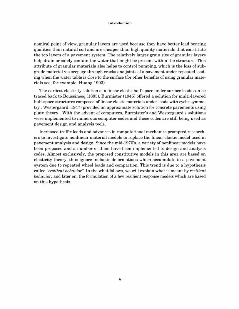
nomical point of view, granular layers are used because they have better load bearingqualities than natural soil and are cheaper than high quality materials that constitutethe top layers of a pavement system. The relatively larger grain size of granular layershelp drain or safely contain the water that might be present within the structure. Thisattribute of granular materials also helps to control pumping, which is the loss of sub-grade material via seepage through cracks and joints of a pavement under repeated load-ing when the water table is close to the surface (for other benefits of using granular mate-rials see, for example, Huang 1993).
The earliest elasticity solution of a linear elastic half-space under surface loads can betraced back to Boussinesq (1885). Burmister (1945) offered a solution for multi-layeredhalf-space structures composed of linear elastic materials under loads with cyclic symme-try . Westergaard (1947) provided an approximate solution for concrete pavements usingplate theory . With the advent of computers, Burmister’s and Westergaard’s solutionswere implemented to numerous computer codes and these codes are still being used aspavement design and analysis tools.
Increased traffic loads and advances in computational mechanics prompted research-ers to investigate nonlinear material models to replace the linear elastic model used inpavement analysis and design. Since the mid-1970’s, a variety of nonlinear models havebeen proposed and a number of them have been implemented to design and analysiscodes. Almost exclusively, the proposed constitutive models in this area are based onelasticity theory, thus ignore inelastic deformations which accumulate in a pavementsystem due to repeated wheel loads and compaction. This trend is due to a hypothesiscalled “resilient behavior”. In the what follows, we will explain what is meant by resilientbehavior, and later on, the formulation of a few resilient response models which are basedon this hypothesis.
5
Chapter 2
An Analysis and Implementation of ResilientModulus Models of Response of Granular Solids
2.1 IntroductionResilient modulus models, like K�� and Uzan–Witczak, are popular material modelsused in analysis and design of pavement systems. These constitutive models are moti-vated by the observation that the granular layers used in pavement construction shake-down quickly to elastic response under the repeated loading that is typically felt by thesesystems. Due to their simplicity, their great success in organizing the response data fromcyclic triaxial tests, and their success relative to competing material models in predictingthe behavior observed in the field, these models have been implemented into many com-puter programs used by researchers and design engineers. This chapter provides a care-ful analysis of the behavior of these models and addresses the issue of effectively imple-menting them in a conventional nonlinear 3–dimensional finite element analysisframework. Also, we develop bounds on the material parameters and present two com-petitive methods for global analysis with these models.
2.1.1 Resilient Behavior and Formulation
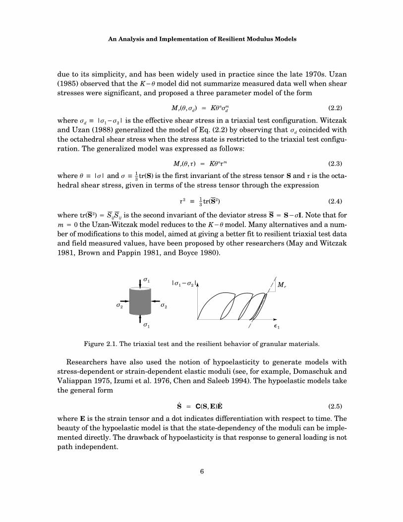
It is generally accepted that granular materials shake down to resilient (elastic) behaviorunder repeated loading (Allen 1973, Huang 1993). The response of a granular soil sampleunder repeated loading is shown schematically for a typical triaxial load test in Figure2.1. Initially, the sample experiences inelastic deformations. The amount of plastic flowdecreases with cycling until the response is essentially elastic. In the literature the “resil-ient modulus” Mr, which is the ratio of the deviator stress to the axial strain at shake-down, is recorded. Extensive efforts have been made to characterize the resilient modu-lus with the associated stress state. Perhaps the earliest model is the so-called K��
model which suggests that the resilient modulus is proportional to the absolute value ofthe mean stress raised to a power, or
Mr(�) � K�n (2.1)
where � �13 |�1�2�2| is the mean pressure acting on the sample in a triaxial test (Hicks
and Monismith 1971). The K�� model has become a very popular material model, partly
An Analysis and Implementation of Resilient Modulus Models
6
due to its simplicity, and has been widely used in practice since the late 1970s. Uzan(1985) observed that the K�� model did not summarize measured data well when shearstresses were significant, and proposed a three parameter model of the form
Mr(�, �d) � K�n�
md (2.2)
where �d � |�1��2| is the effective shear stress in a triaxial test configuration. Witczakand Uzan (1988) generalized the model of Eq. (2.2) by observing that �d coincided withthe octahedral shear stress when the stress state is restricted to the triaxial test configu-ration. The generalized model was expressed as follows:
Mr(�, �) � K�n�
m (2.3)
where � � |�| and � �13 tr(S) is the first invariant of the stress tensor S and � is the octa-
hedral shear stress, given in terms of the stress tensor through the expression
�2�
13 tr(S2) (2.4)
where tr(S2) � SijSij is the second invariant of the deviator stress S � S��I. Note that form � 0 the Uzan-Witczak model reduces to the K�� model. Many alternatives and a num-ber of modifications to this model, aimed at giving a better fit to resilient triaxial test dataand field measured values, have been proposed by other researchers (May and Witczak1981, Brown and Pappin 1981, and Boyce 1980).
�1
�1
�2�2
|�1��2|
�1
Mr
Figure 2.1. The triaxial test and the resilient behavior of granular materials.
Researchers have also used the notion of hypoelasticity to generate models withstress-dependent or strain-dependent elastic moduli (see, for example, Domaschuk andValiappan 1975, Izumi et al. 1976, Chen and Saleeb 1994). The hypoelastic models takethe general form
S.� �(S, E)E
.(2.5)
where E is the strain tensor and a dot indicates differentiation with respect to time. Thebeauty of the hypoelastic model is that the state-dependency of the moduli can be imple-mented directly. The drawback of hypoelasticity is that response to general loading is notpath independent.
Chapter 2
7
2.1.2 Current Approach to Implementation
There are a number of computer programs specifically developed to perform analyses ofpavement systems and these can be listed under three main categories:
i. Multi-layered linear elastic analysis programs based on elastic half-spacesolutions originally presented by Boussinesq (1885) and later generalized tomultiple layers by Burmister (1945) like CHEVRON–ELP (Warren and Dieck-man 1963), BISAR (De Jong, et al. 1972), and ELSYM5 (Kooperman et al.1986).
ii. Multi-layered nonlinear elastic half-space analysis programs like KENLAYER(Huang 1993).
iii. Finite element analysis programs like ILLIPAVE (Raad and Figueroa 1980),MICHPAVE (Harichandran et al. 1971), GTPAVE (Tutumluer 1995), and SENOL(Brown and Pappin 1981).
The computer programs listed above under each category are very similar in all aspectsbut differ only in the way they handle specific issues such as treatment of the domainextent, tension in the granular layers, computation of resilient modulus, considerationof the self–weight of the pavement system, etc. (for detailed descriptions see references).The programs listed under categories 2 and 3 use K��, Uzan–Witczak and similar consti-tutive models. These nonlinear material models have been traditionally implemented asfixed-point iterations wherein initial values of the resilient moduli are assumed, a linearanalysis of the problem is performed using the current values of resilient moduli (as ifthey were constant), and the resulting displacements are used to compute strains, subse-quently stresses, and subsequently new values of the resilient moduli. The process is re-peated until the next computed resilient moduli are equal to the assumed resilient modu-li of the previous iteration. In some of the programs (e.g., KENLAYER) the axisymmetricgranular layers are divided into a rather arbitrary number of sublayers. This is done inorder to take into account the hypothetical variation of resilient modulus with respect todepth, since as depth increases, the influence of the applied loading decreases. (KENLAY-ER also uses a scheme to take into account the horizontal variation of the resilient modu-lus within each layer). Several researchers have chosen to apply to load incrementallyto overcome convergence problems (Huang 1993, Harichandran et al. 1971).
The procedure outlined above is not efficient for several reasons. Every element ineach layer is under a different state of stress, therefore a procedure that accounts for thecontinuous variation of resilient modulus is appropriate. Layered elastic system analysisprograms cannot achieve this end without certain ad hoc modifications (Huang 1993).The convergence of a fixed point iteration is not guaranteed in general even if a uniquesolution to the nonlinear problem exists (Heath 1997) and may require ad hoc treatmentof the problem at hand to obtain a solution. Indeed many researchers report of conver-
An Analysis and Implementation of Resilient Modulus Models
8
gence problems and some, for example, use damping factors when updating the resilientmoduli (Brown and Pappin 1981, Tutumluer 1995).
In what follows, we will develop a strain–based formulation of K�� and Uzan–Witczakmodels which can be implemented directly to a conventional finite element analysis pro-gram. We will then investigate the convergence properties of various implementationsof these two models and make comparisons between the solution technique summarizedabove and more conventional techniques such as Newton’s method.
2.2 Consistent ImplementationThe conventional finite element analysis method is a natural setting for examining theissues associated with the implementation of the K– � and Uzan-Witczak models in threedimensions. In this section we show how the typical extension of these types of modelsto three dimensions allows one to express the stress-dependent resilient moduli com-pletely in terms of strain invariants, obviating the need to solve the nonlinear constitu-tive equations iteratively. We next find closed-form expressions for the eigenvalues of thematerial tangent tensor for the Uzan-Witczak model, and find bounds on the materialparameters required for unique solutions to boundary value problems. We show thatthere are strain states where uniqueness of solution fails.
2.2.1 Notation
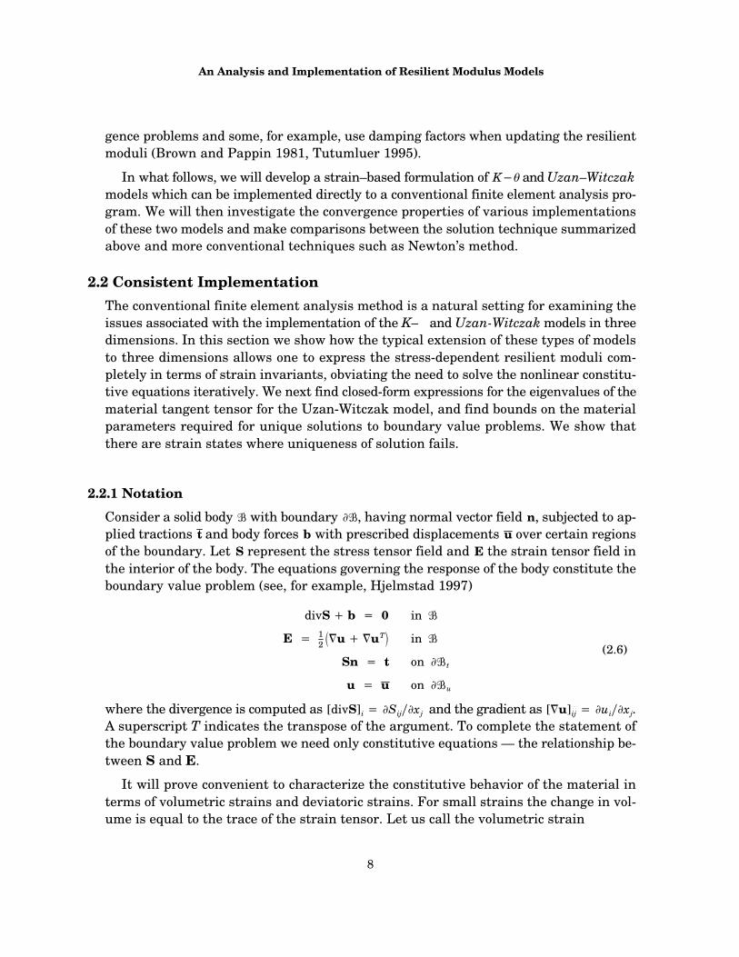
Consider a solid body � with boundary ��, having normal vector field n, subjected to ap-plied tractions t and body forces b with prescribed displacements u over certain regionsof the boundary. Let S represent the stress tensor field and E the strain tensor field inthe interior of the body. The equations governing the response of the body constitute theboundary value problem (see, for example, Hjelmstad 1997)
divS � b � 0
Sn � t
E � 12��u ��uT�
u � u
in �
in �
on ��t
on ��u
(2.6)
where the divergence is computed as [divS]i � �Sij��xj and the gradient as [�u]ij � �ui��xj.A superscript T indicates the transpose of the argument. To complete the statement ofthe boundary value problem we need only constitutive equations — the relationship be-tween S and E.
It will prove convenient to characterize the constitutive behavior of the material interms of volumetric strains and deviatoric strains. For small strains the change in vol-ume is equal to the trace of the strain tensor. Let us call the volumetric strain

Chapter 2
9
� � tr(E) (2.7)
Note that � is an invariant of the strain tensor. The strain deviator can then be definedas
E � E � 13 �I (2.8)
where I is the identity tensor. The octahedral shear strain � is the second invariant ofthe deviatoric strain and is defined through the relationship
�2 � 13 tr(E2) � 1
3 EijEij (2.9)
The deviatoric stress can be defined as S � S��I and one can observe that the octahedralshear stress then obeys 3�2 � tr(S2) � SijSij.
As a point of departure, we note that the linear hyperelastic (Hookean) material hasthe following constitutive equations
S � E1��
(��I � E) (2.10)
where E is Young’s modulus, � is Poisson’s ratio, and �(�) � ��(1�2�) is a parameter thatdepends only on Poisson’s ratio.
2.2.2 Resilient Modulus in Terms of Strains
Both K�� and Uzan–Witczak models describe only a stress dependent modulus of thematerial, and do not, per se, define a constitutive relationship. In the literature (see, forexample, Hicks and Monismith 1971, Uzan 1985) a constitutive model is often postulatedwherein the constant E of the classical Hookean material, Eq. (2.10), is simply replacedwith the resilient modulus Mr. Letting C(�, �) � Mr(�, �)�(1��) we can write this constitu-tive relation as
S � C(�, �)(��I � E) (2.11)
In the context of displacement-based finite element analysis, the constitutive equationscan be viewed as strain driven in the sense that one iterates from an approximate dis-placed configuration Ui to the next Ui�1, where the notation Ui means the nodal displace-ments on a finite element mesh at iteration i, by solving some global equationsUi�1 � G(Ui). The specific issues associated with solving these global equations will beexamined in a later section. For all of these approaches to solving the global problem onecan observe that, upon estimating the new state Ui�1, one can evaluate the strains ineach element. At the local (element gauss point) level we view the solution of the constitu-tive equations as a problem of finding the stress state that corresponds with the strainstate dictated by the global state U. The stresses and the element constitutive matrix are
An Analysis and Implementation of Resilient Modulus Models
10
needed for the computations in the next iteration. For the strain driven problem, we canview the determination of the stress state as finding the roots, i.e., g(S) � 0, of the nonlin-ear function
g(S) � S � C(�, �)(�I � E) (2.12)
for a given state of strain E (and hence given and �). Note that the function g(S) is anonlinear function of S through the nonlinear function C(�(S), �(S)).
Finding the stress state from Eq. (2.12) would be trivial if the resilient modulus C(�, �)could be expressed as a function of strain rather than stress. For the given power lawmodel of resilient modulus we can find such a function. Let us first decompose Eq. (2.12)into bulk and deviatoric parts by letting g � g � 1
3(trg)I and observing that both trg � 0
and g � 0, giving the equivalent equations
� � �C(�, �), S � C(�, �)E (2.13)
where � � (1��)�3(1�2�) � ��1�3. If we define � � || and observe that tr�g2�� 0 weget
� � �C(�, �)�, � � C(�, �)� (2.14)
Letting k � K�(1��), substituting for C(�, �) in Eqn. (2.14) we arrive at the two equations
�n�1�m � 1k��
, �n�m�1 � 1k�
(2.15)
These equations can be solved by observing that Eq. (2.15) implies that � � (����)�. Sub-stituting back into the two original equations and solving for � and � in terms of � and� we get
� � k�(��)�(1�m)��m
� � k�(��)�n��(1�n)(2.16)
where � � 1�(1�n�m). Substituting these results into the definition of the resilient mo-dulus we find that
C(�, �) � C^(�, �) � (k�n�n�m)� � k
^��n��m (2.17)
where k^ � (k�n)� is the constant for the strain-based formulation of the stress-dependentmoduli. Note that when the exponent m is set equal to zero we can recover the relevantexpressions for the K�� model. In terms of strains, the constitutive equation (2.11) be-comes
S � C^(�, �)(�I � E) (2.18)
With this equation, the strain-driven constitutive equations are trivial to solve. We shalltake Eq. (2.18) as the basic statement of the K�� and Uzan–Witczak models for the re-mainder of this study.

Chapter 2
11
2.2.3 Material Tangent Stiffness
The material tangent stiffness C � �S��E can be computed directly from Eq. (2.18) as
�S�E � C
^(1 � �I � I) � (��I � E) ��EC^
(2.19)
where we have recognized that ����E � I (with components [I]ij � �ij) and that �E��E � 1(with components [1]ijkl � �ij�kl). Because � � |�|, we can compute
���E �
����
���E � sgn(�)I (2.20)
and because �2 � 13 EijEij, we can compute
���E � 1
3E� (2.21)
With these definitions, we find that
�EC^(E) � �C
^
�����E ��C
^
�����E � �C
^�n� I � m
3�2 E (2.22)
Letting N � E�� we arrive at the final expression for the material tangent stiffness C forthe K�� and Uzan–Witczak models
C � C^(�, �)1 � ��n��� I � I �
�m3 N � N �
���m3� I � N �
��n� N � I� (2.23)
Notice that this tensor is not symmetric, and has skew part
Cskew ��C
^
6�����2m � 3�2n [I � N � N � I] (2.24)
The material tangent stiffness tensor is useful for both for finding bounds on the mate-rial parameters of the model and also for carrying out numerical computations. In partic-ular, it can be used to find the tangent stiffness matrix. Using standard notions of assem-bly of the stiffness matrix, the tangent stiffness matrix can be computed as
Kt(U) � �Mm�1
�m
BTm(x)Cm(U, x)Bm(x) dV (2.25)
where M is the number of elements, �m is the region occupied by element m, and Cm(U, x)is the material tangent tensor for element m, which depends upon the displaced state Uand varies with the spatial coordinates x. The strain-displacement matrix Bm allows thecomputation of the strain tensor in element m from the nodal displacement U as
Em(x) � Bm(x)U (2.26)
An Analysis and Implementation of Resilient Modulus Models
12
2.2.4 Uniqueness and Path IndependenceUniqueness of the equilibrium configurations displayed by the constitutive models canbe assessed with a simple argument using the principle of virtual work. The principle ofvirtual work states that, if the equation
��
S � E^ dV � ���
t � u^ dA � ��
b � u^ dV (2.27)
holds for all arbitrary kinematically admissible virtual displacement fields u^ and theircorresponding strain fields E^ , then equilibrium is satisfied in the domain and on theboundary (see, for example, Hjelmstad 1997A). Therefore, if the traction forces t andbody forces b acting on body � are incremented by amounts �t and �b, respectively, witha resulting displacement increment �u, then the resulting increments in stress �S andstrain �E.
Following Sokolnikoff (1956), let us assume that there are two distinct equilibriumstates (I and II) corresponding to the increments �t and �b and given by �SI and �SII. Sub-stituting the stress states S��SI and S��SII into Eqn. (2.27), taking the difference, andparticularizing to the virtual strain E^ � �EI��EII, where �EI and �EII are the strainsassociated with the stress states �SI and �SII, we find that
��
�SI��SII � �EI��EII dV � 0 (2.28)
Denoting the differences in states as S *� �SI��SII and E *� �EI��EII, and substitutingthe incremental constitutive equation S *� CE *, Eqn. (2.28) becomes
��
E * � CE * dV � 0 (2.29)
Therefore if C is positive definite, then the strain state differences E *, and thus the stressstate differences S *, are identically zero. Thus, uniqueness of solution depends upon thedefiniteness of the tensor C. A positive definite tensor is one that has all positive eigenva-lues. Hence, we must examine the eigenvalues of the material tangent tensor.
2.2.5 Eigenvalues of the Material Tangent Tensor
Eqn. (2.29) indicates that uniqueness of stress for a given strain state (or vice versa) isguaranteed if the material tangent stiffness tensor C is positive definite. This restrictionimposes certain bounds on the material constants of the K�� and Uzan–Witczak models.
Let us obtain the eigenvalues and eigenvectors, for a tensor of the form
T � 1 � aI � I � bN � N � cI � N � dN � I (2.30)
Chapter 2
13
where, a, b, c, and d are scalars. If � is an eigentensor of T, with eigenvalue �, then
T� � �� [a(I � �) � c(N � �)]I � [d(I � �) � b(N � �)]N � �� (2.31)
The tensor � is symmetric (it has the same character as the strain tensor). Therefore,there are 6 eigenvectors. Four of these tensors (�(3), �(4), �(5), �(6)) correspond to a repeatedeigenvalue because these tensors need only be orthogonal to I and N. Therefore, � � 1is an eigenvalue of algebraic multiplicity 4
�3 � �4 � �5 � �6 � 1 (2.32)
The remaining two eigentensors must lie in the subspace spanned by tensors I and N.To wit, the remaining eigenvectors are of the form
� � I � �N (2.33)
Because N � E��, we have I � N � �ijNij � 0. Hence, these tensors are orthogonal in thissense. Substituting Eq. (2.33) into Eq. (2.31), noting that I � I � 3 and N � N � 3 andequating the coefficients of I and N, we get the following equations for � and �
��1 � 3a � 3�c
�(��1) � 3d � 3�b(2.34)
Multiplying the first of these by � and subtracting the result from the second we arriveat a quadratic equation for �
c�2 � (a�b)�� d � 0 (2.35)
Solution of this quadratic equation yields the two parameters �1 and �2
�1,2 �b�a � (a�b)2 � 4cd
2c (2.36)
These values of � can be substituted back into Eq. (2.34)a to give the remaining eigenva-lues
�1,2 � 1 � 32�b�a � (a�b)2 � 4cd � (2.37)
From Eq. (2.23) we can identify the constants as
a � �n�� �, b � �m�3, c � �m���3�, d � �n��� (2.38)
With these values, and noting that C � C^T we find the eigenvalues of C to be
�1,2 � C^�1,2, �3,4,5,6 � C
^(2.39)
The tensor C is not symmetric, but it is easy to show that the eigenvalues of CT are identi-cal to the eigenvalues of C.
An Analysis and Implementation of Resilient Modulus Models
14
For uniqueness of solution we must have �i � 0, for i�1, . . ., 6, and from this require-ment bounds on the material constants can be established. It is interesting to note that�1,2 do not depend upon the state of strain because a, b, and c, d depend only upon the material parameters. Therefore, the dependence of the eigenvalues of C comes entirelyfrom C^(�, �), which is a multiplier for all six of the eigenvalues. Therefore, the form of thespectrum is constant and loss of uniqueness can occur only when C^(�, �) � 0. As a conse-quence, we can observe that bounds on the material parameters �, n, and m imposed bythe requirement of uniqueness of solution are
�1,2 � 1 � 32b�a � (a�b)2 � 4cd� � � 0 (2.40)
A somewhat lengthy, but straightforward, calculation shows that �1,2 � 0 if and only if
�� � 0 (2.41)
Clearly, then we must have n�m � 1 and � � 0, which implies �1 � � � 1�2. If the pa-rameters of the model are chosen to satisfy Eq. (2.41) then the solution can fail to beunique only for states of strain where � � 0 or � � 0.
2.3 Solution MethodsIn this section we analyze the iterative methods currently used for pavement analysisand show that, because the constitutive model hardens, these iterative methods arebound to eventually fail. Finally, we make some comparisons with Newton-type solutionmethods and modified Newton methods on some example problems.
As mentioned earlier, fixed-point iteration is traditionally the method of choice in solv-ing boundary value problems of pavement systems having layers that display nonlinearmaterial behavior. In this section we will investigate the convergence properties of sucha method on a single finite element with one integration (material) point. This is a verysimple problem, however it will enable us to gain insight to the convergence propertiesof this iterative solution method when applied to a collection of material points ( i.e., In-tegration points in a finite element mesh) which behave according to the constitutiverelations given by K�� or Uzan–Witczak Models.
The principle of virtual displacements suggests that equilibrium is satisfied if
�(U) � Mm�1
�m
BTmSm(U) dV � P � 0 (2.42)
where U are the nodal displacements, P are the work equivalent nodal loads, Bm is thestrain-displacement operator for element m, defined in Eq. (2.26), and Sm(U) is the stressin element m, which depends upon the nodal displacements through the strains. Thesummation in Eq. (2.42) is the usual assembly procedure and the element integrals are
Chapter 2
15
generally carried out with numerical quadrature. The subscript m on the stress tensorSm(U) indicates that the stress field is localized to element m. The stress field is said todepend upon the nodal displacements because, for a given displacement state, the strainsare computed from the displacements in accord with Eq. (2.26) and the invariants � and� are computed from the strains. In this sense, the computation is strain driven. In thefollowing sections we shall discuss and analyze various methods for solving two and threedimensional problems using this constitutive model.
2.3.1 Secant MethodOne can define a secant stiffness matrix at a given state U by computing
Ks(U) � �Mm�1
��m
BTmDm(U)Bm dV (2.43)
where the material secant stiffness is defined as
D � C^(�, �)1 � �I � I (2.44)
The only difference between the tangent stiffness and the secant stiffness matrix of Eq.(2.43) is that in the tangent stiffness we used the consistent material tangent modulusC defined in Eq. (2.23) whereas in the secant stiffness we use the surrogate modulus Ddefined in Eq. (2.44)
Perhaps the simplest version of the fixed-point iteration is
Ui�1 � K�1s (Ui)P (2.45)
which can be started with an initial displacement vector U0. In practice one does not spec-ify an initial guess of displacements, but rather an initial distribution of the modulus C^ 0.Using this initial modulus the first iteration gives the initial displacement approxima-tion and the iteration proceeds as given above. We shall refer to the algorithm of Eq.(2.45) from here on as the total (original) secant method.
The fixed-point iteration described by Eq. (2.45) is in the form Ui�1 � G(Ui), and willconverge if the spectral radius of �G(U*) is less than unity at the solution U*. Noting thatthat at the solution we have K�1
s (U*)P � U* we find that
�G(U*) � �K�1s (U*)�Ks(U*)U* (2.46)
where the gradient of the inverse of a matrix was computed by noting K�1K � I. The gra-dient of the secant stiffness matrix can be computed from Eq. (2.43), noting thatBmU � Em, by noting that
�Ks(U)U � �Ks
�U U � �Mm�1
��m
BTm�UDm(U)Em dV (2.47)
An Analysis and Implementation of Resilient Modulus Models
16
where UD can be computed via the chain rule for differentiation as
UD � �D�U � �D
�E�E�U � �D
�E B (2.48)
Noting that we can compute the stress from the secant relationship S � DE, we can ob-serve that
C � �S�E �
�(DE)�E � �D
�E E � D (2.49)
It therefore follows that
�D�E E � C � D (2.50)
Therefore, combining Eqn.’s (2.47), (2.48), and (2.50), we find that
Ks(U)U � �Mm�1
�m
BTm[Cm(U) � Dm(U)]Bm dV (2.51)
Thus, Ks(U)U � Kt(U) � Ks(U) and the gradient of the fixed-point iteration function ofEq. (2.46) reduces to
G(U*) � I � K�1s (U*)Kt(U*) � A (2.52)
The spectral radius of A is the largest eigenvalue of A. Let the eigenvalue problem bedenoted as Aa � �a, where � is the (possibly complex valued) eigenvalue and a is theassociated eigenvector. Then the criterion for convergence of the fixed-point iteration is
r(A) � �max � 1 (2.53)
where r(�) is the spectral radius of (�), and where �max is the modulus of the largest eigen-value of A. Observe that when the secant stiffness is close the the tangent stiffness�max � 0 and convergence of the iteration is very rapid (nearly quadratic). As the secantand tangent stiffness grow apart, as they do with increasing deformation, the eigenva-lues of A get increasingly negative because the tangent is always steeper than the secantfor this model. Therefore, the fixed-point iteration is eventually bound to diverge if theload level is high enough.
2.3.2 Damped Secant Method
Researchers have observed that the fixed-point iteration described in the previous sec-tion has poor convergence properties (Brown and Pappin 1981, Tutumluer 1995). Theconvergence properties of this method were observed to improve with the introductionof a “damped” fixed-point iteration in which a secant modulus is formed from the currentstate and the previous state using an effective modulus
Chapter 2
17
C � �C^(Ui) � 1���C
^(Ui�1) (2.54)
where the damping parameter � � [0, 1] is selected a priori. Tutumluer (1995) has re-ported that a value of � � 0.8 gives good results. Note that, for notational convenience,we consider C^ to be a function of the state U. Using C in the definition of the secant mate-rial modulus, Eq. (2.44), and using that in the definition of the global secant stiffness, Eq.(2.43), we find that the result is a modified secant stiffness
K(Ui, Ui�1) � �Ks(Ui) � 1���Ks(Ui�1) (2.55)
This modified stiffness is then used to define a modified fixed-point iteration as
K(Ui, Ui�1)Ui�1 � ��Ks(Ui) � 1���Ks(Ui�1)Ui�1 � P (2.56)
We shall refer to the algorithm of Eq. (2.56) from here on as the total damped secant meth-od.
To examine the convergence properties of this fixed-point iteration it is convenient toput it into the form Z � G(Z), from which we can observe that r(�ZG) � 1 is the criterionfor convergence. The two-step iteration for Eq. (2.56) can be converted to a one-step itera-tion by introducing the variable Wi�1 � Ui. Now we can write the iteration as
K(Ui, Wi) 00 I
Ui�1
Wi�1
PUi� (2.57)
If we define Zi �{Ui, Wi} then we can identify the function G(Z) from Eq. (2.57) as
�K(Ui, Wi)�1
PUi
G(Zi) � (2.58)
The gradient of G can be computed as
��K�1��UKsK
�1P
0�ZG(Zi) �
I�1���K
�1��WKsK�1
P (2.59)
The convergence criterion is expressed in terms of the spectral radius of �ZG evaluatedat the solution U � W � U*. At this point, K�1
P � U* and K � Ks. Consequently,
�A0
�ZG(Z*) �I
1���A(2.60)
where A � I�K�1s Kt, from Eq. (2.51). The eigenvalues � of �ZG are determined from the
eigenvalue problem
�A0I
1���Aba
ba
� � (2.61)

An Analysis and Implementation of Resilient Modulus Models
18
The bottom partition of this equation gives a � �b. Substituting this into the top parti-tion we find that
��� 1��1��Aa � �a (2.62)
Thus, we can observe that a is an eigenvector of A. If � is the corresponding eigenvalueof A, i.e., it satisfies the eigenvalue problem Aa � �a, then the eigenvalue of the systemin Eq. (2.61) is related to � as
� � �2
��� �1��(2.63)
Observe that when � � 1 the system reverts to the undamped fixed-point iteration of theprevious section and the eigenvalues are the same. Solving Eq. (2.63) for � in terms of� gives
� � 12��� � �2�2 � 4��1�� � (2.64)
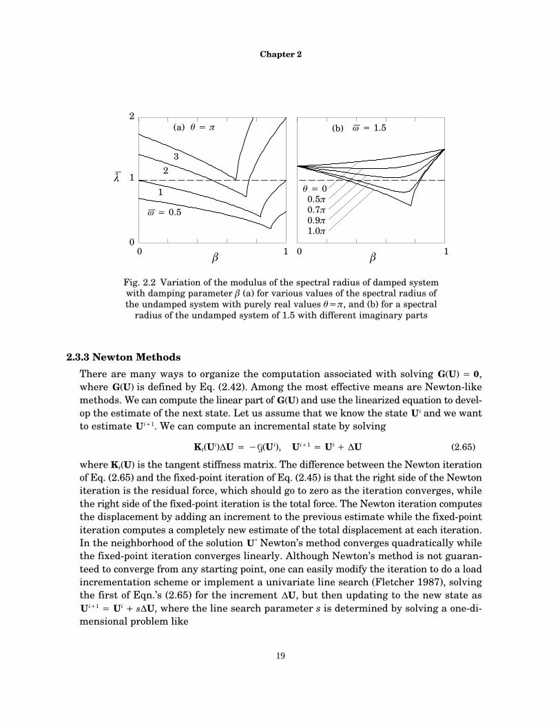
Since the matrix A is not necessarily symmetric its maximum eigenvalue � will generallybe complex valued. Consequently, the eigenvalue of the damped system will also be com-plex valued. The spectral radius of the damped system (i.e., the modulus of �) is shownas a function of the damping parameter � in Fig. 2.2 for values values of the eigenvalue� � �e i�. It is apparent from this figure that a damped secant method will converge incases where an undamped case will not (up to � � 3 in the best case) and that it will im-prove the convergence characteristics in all cases where the undamped secant methodwill converge. Furthermore, the presence of an imaginary part to the eigenvalue of A willalways blunt the ability of the damped method to improve convergence. For example,with � � 1.5 no improvement can be achieved through damping if � � 0.5. The optimalvalue of damping depends on both the magnitude and phase of the eigenvalue of the un-damped case, which is not known a priori.
Chapter 2
19
32
1
� � 0.5
0 1
1
2
0
0.5�0.7�0.9�1.0�
� � 0
0 1
�
� �
Fig. 2.2 Variation of the modulus of the spectral radius of damped systemwith damping parameter � (a) for various values of the spectral radius ofthe undamped system with purely real values ���, and (b) for a spectral
radius of the undamped system of 1.5 with different imaginary parts
(b) � � 1.5� � �(a)
2.3.3 Newton MethodsThere are many ways to organize the computation associated with solving G(U) � 0,where G(U) is defined by Eq. (2.42). Among the most effective means are Newton-likemethods. We can compute the linear part of G(U) and use the linearized equation to devel-op the estimate of the next state. Let us assume that we know the state Ui and we wantto estimate Ui�1. We can compute an incremental state by solving
Kt(Ui)�U � ��(Ui), Ui�1� Ui
� �U (2.65)
where Kt(U) is the tangent stiffness matrix. The difference between the Newton iterationof Eq. (2.65) and the fixed-point iteration of Eq. (2.45) is that the right side of the Newtoniteration is the residual force, which should go to zero as the iteration converges, whilethe right side of the fixed-point iteration is the total force. The Newton iteration computesthe displacement by adding an increment to the previous estimate while the fixed-pointiteration computes a completely new estimate of the total displacement at each iteration.In the neighborhood of the solution U* Newton’s method converges quadratically whilethe fixed-point iteration converges linearly. Although Newton’s method is not guaran-teed to converge from any starting point, one can easily modify the iteration to do a loadincrementation scheme or implement a univariate line search (Fletcher 1987), solvingthe first of Eqn.’s (2.65) for the increment �U, but then updating to the new state asUi�1
� Ui� s�U, where the line search parameter s is determined by solving a one-di-
mensional problem like

An Analysis and Implementation of Resilient Modulus Models
20
mins
� �(Ui�s�U) � (2.66)
Another popular line search criterion is to solve �UT�(Ui�s�U) � 0 for the line search pa-rameter s (Crisfield 1991).
A modified Newton iteration can be established by replacing the tangent stiffness withthe secant stiffness in Eq. (2.65) to give
Ks(Ui)�U � ��(Ui), Ui�1 � Ui � �U (2.67)
where Ks is defined in Eq. (2.43). The stiffness matrix used in Newton-like iterations af-fects only the convergence properties of the algorithm not the converged solution. Astraightforward analysis of this algorithm as a fixed-point iteration shows that its con-vergence properties are exactly the same as the original (total) secant method. Further,one can show that using the damped secant does not improve the convergence character-istics like it did for the original (total) secant method. On the other hand, a line searchcan be used in the modified Newton method of Eq. (2.67), but not in the secant methodof Eqn. (2.45) or the damped secant method of Eq. (2.56).
From here on we shall refer to the finite element formulation based on Eqn. (2.65) asthe incremental tangent formulation and the finite element formulation based on Eqn.(2.67) as the incremental secant formulation.
In what follows, we will investigate convergence properties of the solution techniquesdescribed so far on example problems and try to identify the best strategies for the solu-tion of nonlinear finite element equations.
2.4 Simulations and Convergence StudiesWe have implemented the algorithms discussed earlier to the commercial finite elementpackage ABAQUS (1994) with the help of user defined subroutine UMAT. The programABAQUS supports both symmetric and non-symmetric tangent formulations as well asline searches. A brief overview of ABAQUS UMAT routines and the source code of theimplementation of the methods described above can be found in Appendix I and AppendixII.
2.4.1 Triaxial Test Simulation
In order to compare the various algorithms presented in this chapter we shall use themto compute the response of the simulated triaxial test configuration shown in Fig. 2.4.The model was constrained against vertical movement at the bottom, but allowed fric-tionless sliding on the top and bottom faces. Tractions were applied on the lateral sur-faces of the test piece. The material properties were K � 118.6 MPa, n � 0.4, and m � 0.3,which are representative of a moderate to loose granular material. The extent of nonlin-

Chapter 2
21
earity can be observed from the plot of the proportional load factor versus average strainin Figure 2.3. In particular, this degree of nonlinearity should be sufficient to exhibit thedifferences among the various algorithms.
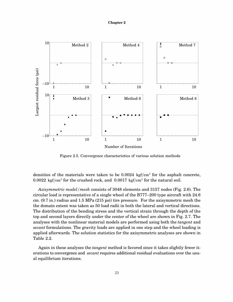
The results of analysis of the triaxial sample under five different load levels are shownin Table 2.1. In each case the total load was applied in a single step and the state wasiterated to convergence until default ABAQUS criteria were satisfied (ABAQUS, 1994).The algorithms used either secant stiffness matrix or a tangent stiffness matrix. The se-cant was either damped ( � � 0.8) or original ( � � 1). The tangent was either the unsym-metrical consistent or symmetrized consistent tangent. For each of these four choices thecomputation was done with and without line search. The table gives the number of itera-tions required for convergence at each load level. The typical convergence characteristicsfor the convergent methods are shown in Fig. 2.5.
The original secant method without line search failed to converge for all load levels.The beneficial effects of line search and damping can be seen in methods 2 and 3. Linesearch is considerably better than damping, but requires additional effort. Interestingly,damping and line search together is actually worse than line search alone. The symme-trized tangent stiffness method failed to converge at all load levels, while the unsymmet-rical tangent stiffness method converged well at all load levels. It is interesting to notethat the lowest load level was the most difficult for the consistent tangent, possibly be-cause stiffness levels are so low for that load level (the secant being greater than the tan-gent there). Line search helped both tangent methods. The unsymmetrical tangentmethod appears to be competitive with the original secant method with line search interms of number of iterations to convergence, but is considerably more expensive per it-eration to compute. It would appear that the best strategy in this example is the original
7 � 10�4
15�
3�
Figure 2.3. Finite element mesh and material response of example triaxial test.
30 cm.
15 cm.
3�
Average Strain
� (psi)
6
00

An Analysis and Implementation of Resilient Modulus Models
22
Stiffness Matrix
Sym
Table 2.1. Results of example triaxial test computation for various solution algorithms
DampMethod LS
Orig Unsym 0.33 1 2 3 4
Load Factor �
nc = no convergence
1 – Yes – – – nc nc nc nc nc2 Yes Yes – – – 2 3 3 2 23 – – Yes – – 5 7 5 5 44 Yes – Yes – – 4 5 4 3 35 – – – Yes – nc nc nc nc nc6 Yes – – Yes – 8 10 10 9 97 – – – – Yes 6 4 3 3 38 Yes – – – Yes 3 3 2 3 3
Secant Tangent
secant method with line search. The damped secant method without line search performsreasonably well also.
2.4.2 Axisymmetric Pavement Analysis
For the purpose of demonstration, an axisymmetric finite element analysis was per-formed on a flexible pavement system consisting of three layers of materials. The top lay-er of the system was 20 cm. of asphalt concrete, the second layer was 112 cm. of high den-sity crushed rock, designated as HD1 by Allen (1973) (see Chapter 4), and the bottomlayer was natural soil extending to a depth of 9 m. In the various analyses, the asphaltconcrete layer was assumed to be linear elastic with Young’s modulus E�1380 MPa andPoisson’s ratio of � � 0.35. The natural soil was also assumed to be linearly elastic withYoung’s modulus E�40 MPa and Poisson’s ratio of � � 0.45. The second layer was mod-eled using one of the following models: (a) linear elasticity with E�240 MPa and � � 0.34,(b) K–� with k�420 MPa, n�0.29, and� � � 0.33� and (c) Uzan–Witczak with k�425MPa, n�0.22, m�0.07, and�� � 0.32. The values of the material constants for the highdensity crushed rock material were established by fitting the given model (one of thethree), using a weighted nonlinear least-squares curve fitting technique (as discussed inChapter 4), to the laboratory test data measured by Allen (1973). Thus, although themodels are quite different, they are each an attempt to best fit the given test data. The
Chapter 2
23
Method 2
Method 3
Method 4
Method 6
Method 7
1 10 1 10 1 10
1 10 1 10
–10
10
1 10
Method 8
–10
10
Number of Iterations
Figure 2.5. Convergence characteristics of various solution methods
Lar
gest
res
idua
l for
ce (
psi)
densities of the materials were taken to be 0.0024 kgf�cm3 for the asphalt concrete,0.0022 kgf�cm3 for the crushed rock, and 0.0017 kgf�cm3 for the natural soil.
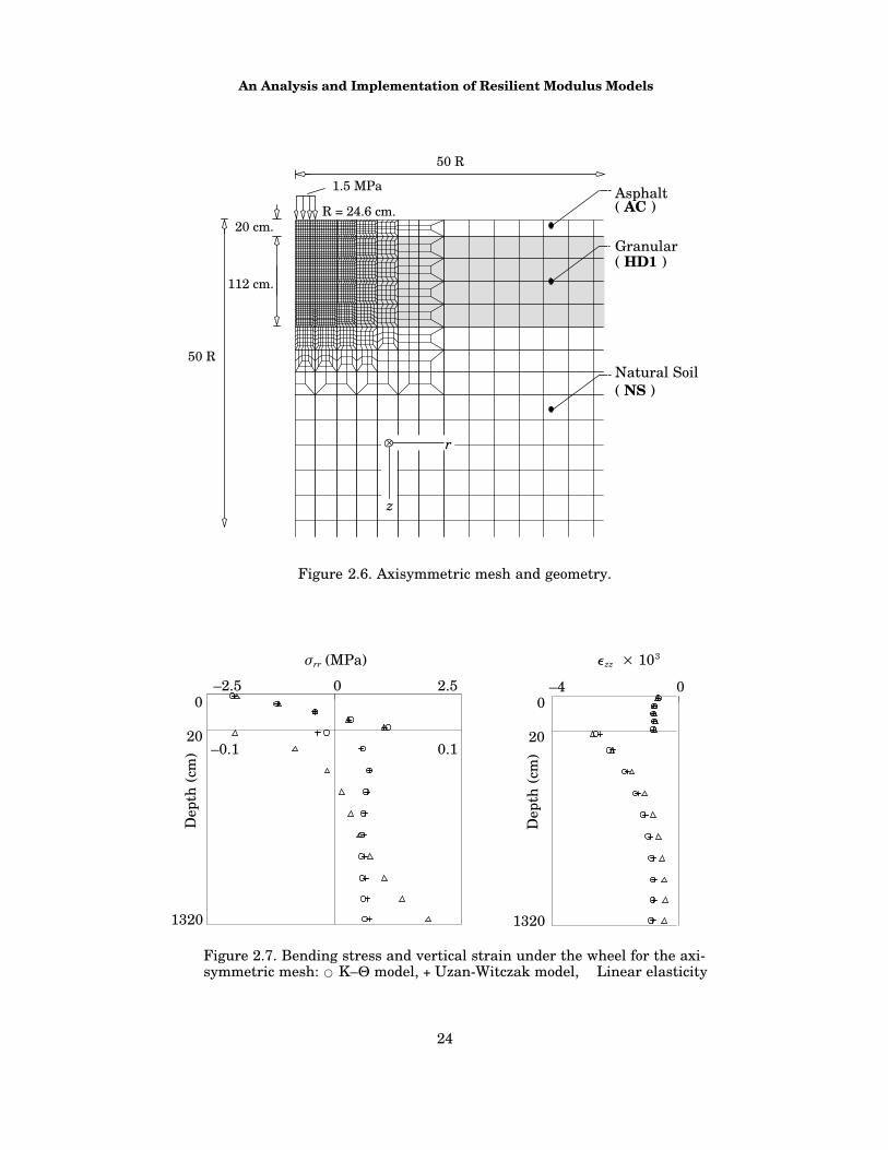
Axisymmetric model/mesh consists of 3048 elements and 3157 nodes (Fig. 2.6). Thecircular load is representative of a single wheel of the B777–200 type aircraft with 24.6cm. (9.7 in.) radius and 1.5 MPa (215 psi) tire pressure. For the axisymmetric mesh thethe domain extent was taken as 50 load radii in both the lateral and vertical directions.The distribution of the bending stress and the vertical strain through the depth of thetop and second layers directly under the center of the wheel are shown in Fig. 2.7. Theanalyses with the nonlinear material models are performed using both the tangent andsecant formulations. The gravity loads are applied in one step and the wheel loading isapplied afterwards. The solution statistics for the axisymmetric analyses are shown inTable 2.2.
Again in these analyses the tangent method is favored since it takes slightly fewer it-erations to convergence and secant requires additional residual evaluations over the usu-al equilibrium iterations.
An Analysis and Implementation of Resilient Modulus Models
24
Figure 2.6. Axisymmetric mesh and geometry.
R = 24.6 cm.20 cm.
112 cm.
50 R
50 R
Asphalt
Granular
Natural Soil
( HD1 )
1.5 MPa
z
r�
( AC )
( NS )
–2.5 2.5
20
0
1320
Dep
th (
cm) –0.1 0.1
0 –4
20
0
1320
Dep
th (
cm)
0
Figure 2.7. Bending stress and vertical strain under the wheel for the axi-symmetric mesh: � K–� model, + Uzan-Witczak model, � Linear elasticity
�rr (MPa) �zz � 103

Chapter 2
25
Table 2.2. Solution Statistics for the Axisymmetric Mesh
MATERIAL
K– �
Uzan–Witzcak
Linear Elastic
SOLUTION
Tangent (7)
–
Secant (2)
Tangent (7)
Secant (2)
METHOD
1 1
4 3
3 5
3 6
4 5
LOAD STEP 1( Grav. Loads )
LOAD STEP 2( Wheel Loads )
EQUILIBRIUM ITERATIONS
MODEL
2.4.3 Three Dimensional Pavement Analysis
For the purpose of demonstration, a 3–dimensional finite element analysis was per-formed on a flexible pavement system consisting of a layer of asphalt concrete on a layerof high density crushed rock, on top of natural soil as shown in Fig. 6.1 (see Chapter 6).The pavement system was subjected to a loading representative of a B777–200 type air-craft tridem gear (FAA 1995). The footprint of the loading is also shown in the same fig-ure. The 55 cm. � 35 cm. rectangular tire prints are assumed to have a uniform pressureloading of 1.5 MPa. The loading was applied to the center of a 32 m � 32 m region. Thefinite element mesh of this analysis is described in Chapter 6 (see Figure 6.2).
The loading was applied in three steps with the gravity loads induced by the weightof materials first followed by two equal increments of the applied gear loads. Equilibriumunder gravity loads was iterated to convergence prior to application of the wheel loads.Obviously, for the linear elastic model, one iteration was needed for each load applica-tion. For the nonlinear models the number of iterations required depends upon the solu-tion strategy used. For this problem we considered only the consistent (unsymmetrical)tangent method without line search (method 7 in Table 2.1) and the original secant meth-od with line search (method 2 in Table 2.1). Solution statistics of these analyses areshown in Table 2.3.
This three–dimensional example shows that the convergence results appear to favorthe consistent tangent without line search over the original secant with line search, butnot by much. The presentation of the stress and strain results for this analysis are def-

An Analysis and Implementation of Resilient Modulus Models
26
erred to appear in Chapter 6 in which we compare the predictions of various other resil-ient models as well as the ones that are presented in this chapter.
Table 2.3. Solution Statistics for the Three–Dimensional Mesh
MATERIAL
K– �
Uzan–Witzcak
Linear Elastic
LOAD STEP 1( Grav. Loads )
LOAD STEP 2( Wheel Loads )
EQUILIBRIUM ITERATIONSSOLUTION
Tangent (7)
–
Secant (2)
Tangent (7)
Secant (2)
METHOD
1 1
4 3
5 6
5 5
4 3
1
2
6
9
5
Increment 1 Increment 2MODEL
2.5 ConclusionsThe K�� and Uzan–Witczak constitutive models are widely used in pavement analysisto characterize the resilient response of granular materials. The models possess a resil-ient modulus C that depends upon the state of stress. These models have traditionallybeen implemented in finite element programs primarily with the original and dampedsecant methods. Success in computing with these models has been modest at best, andit appears that there has never before been a full three dimensional implementation ofthese models.
In this chapter we have presented a three dimensional analysis and implementationof the Uzan-Witczak constitutive model. We have shown that the resilient modulus,traditionally expressed as a function of stress invariants, can be equivalently cast interms of strain invariants, thereby simplifying element level computations of the stressstate. We have derived the consistent material tangent tensor, which has relevance bothin implementing the ordinary Newton iteration and in proving that this model can sufferfrom loss of uniqueness of solution at various states of stress and strain. We have pres-ented closed form expressions for the eigenvalues and eigenvectors of the material tan-gent tensor, from which bounds on the material constant required for uniqueness of solu-tion were derived. We have presented a careful analysis of the convergence properties ofthe original and damped secant methods and have proven that it is possible for damping

Chapter 2
27
to improve convergence and that there is good reason why a value of the damping param-eter in the neighborhood of � � 0.8, mentioned by other researchers, works well. We haveshown that the modified Newton algorithm using the secant stiffness in place of the tan-gent stiffness has the same convergence properties as the original (total) secant methodand that convergence of the modified Newton method is not improved by damping thestiffness matrix. We have also presented a reformulation of the damped secant methodthat allows implementation of the method in a standard nonlinear finite element analy-sis package. This reformulation also has the benefits that the method can take advantageof load incrementation and line searches.
We illustrated the tradeoffs among eight versions of these algorithms with an exampletriaxial test configuration and a three dimensional analysis of a layered pavement sys-tem. These example suggests that the two best algorithms are ones that have not beenused by other researchers concerned with these constitutive models — the original secantmethod with line search and Newton’s method with a consistent tangent stiffness matrix.While the effort per iteration of these two methods is quite different they appear to becompetitive overall.

28
Chapter 3
A Simple Coupled Hyperelastic Model
3.1 Introduction
Granular materials comprise discrete grains, air voids and water. These attributes leadto complex and often unpredictable behavior of these materials under applied loading.Unlike metals, granular materials tend to change their volume under deviatoric strain-ing, and the shear stiffness of granular materials is affected by the applied mean (com-pressive) stress. Thus, there is a coupling effect between the volumetric and deviatoricresponse of granular materials. Stress induced anisotropy and inability to bear tensilehydrostatic loads are also important characteristics of granular materials to be consid-ered when developing constitutive models to represent their behavior under loading. Athorough discussion of these important features and the accompanying experimental ev-idence can be found elsewhere (see for example, Lade 1988).
The triaxial test data indicate a strong stress dependence of the final shakedown slopeof the cyclic response. Efforts to characterize this elastic behavior, as we have discussedearlier, go back at least to Hicks and Monismith (1971). As noted earlier, there have beenmany subsequent efforts to improve the description of the resilient behavior within thecontext of the resilient modulus and within the framework of hypoelasticity (where astress-dependent modulus is easily implemented). The drawback of these formulationsis that they do not lead to path independent elastic response and some of the models re-quire some leaps of faith when extending them to three dimensional response.
In this chapter we propose a coupled hyperelastic constitutive model to characterizethe resilient behavior of granular materials. The model is developed by adding a simplecoupling term and a nonlinear shear response to the ordinary strain energy density func-tion of linear elasticity. The resulting model is a four parameter model that can be fit totriaxial test data. The model is extended to limit the tensile response of the material un-der the assumption that the pressure should reach a (presumably small) limiting valueas the volumetric strain takes on positive values. The model is implemented in a finiteelement context and compared to other models for a plate loaded pavement and as willbe presented in Chapter 6, for an airport pavement containing a layer whose behavioris governed by the proposed model under applied loading.

A Simple Coupled Hyperelastic Model
29
3.2 FormulationThe framework of hyperelasticity provides a good foundation for developing constitutivemodels to represent the resilient behavior of granular materials. For a hyperelastic mate-rial, the stress is related to the strain through the strain energy density function �(E)by
S � ��(E)�E (3.1)
which, in turn, guarantees path independent response. The hyperelastic model is capableof representing resilient behavior and is suited to large-scale finite element computation.
An uncoupled isotropic hyperelastic constitutive model can be derived from a strainenergy density function of the form �(�, �) � �(�)��(�). In particular, linear isotropicelasticity has the strain energy
�(�, �) � 12 K�
2 � 3G�2 (3.2)
Noting that the relationships ����E � I and ��3�2���E � 2E, the linear elastic constitutiverelationship takes the form
S � K�I � 2GE (3.3)
where K and G are usually called the bulk and shear moduli, respectively. This relation-ship between stress and strain is the familiar Hooke’s Law. The mean pressure and octa-hedral shear stress can be computed from Eqn. (2.10) as
� � K�, � � 2G� (3.4)
It is obvious from Eqns. (3.2) and (3.4) that the volumetric and deviatoric responses areuncoupled.
3.2.1. Coupled Hyperelastic models
A coupling effect can be introduced via a strain energy density function of the form
�(�, �) � 12 K�
2 � 3G�2 � 3
2 b�4 � 3c��2 (3.5)
where K, G, b, and c are material constants. One can see the remnants of linear elasticityin this strain energy function with two additional nonlinear terms. The fourth term givesthe coupling effect. It has been observed experimentally that the response in shear is non-linear even when bulk effects are fixed. Thus, the third term enhances the primary shearresponse strain energy to include a quartic term. Using the definition given in Eqn. (3.1)with the strain energy function given in Eqn. (3.5) we obtain the stress-strain relation-ship

Chapter 3
30
S � �K�� 3c�2�I � �2G � 2b�2 � 2c��E (3.6)
The mean pressure and octahedral shear stress are related to the volumetric and octahe-dral shear strain as
� � K�� 3c�2, � � �2G � 2b�2 � 2c��� (3.7)
The coupling in Eqn. (3.7) is evident. To keep the volume constant under shearing, thepressure must increase. Because Eqn. (3.7) is linear in �, one can relate shear stress toshear strain and mean stress as
� � 2G�1 � cKG
���� 2b�1 � 3c2
Kb��3 (3.8)
From this relationship one can observe two important things. First, the first-order cou-pling feature that leads to increase shear stiffness is evident in the first term. (Rememberthat mean stress is negative in compression). Second, the nonlinear effect representedby the second term suggests that including the term b�4 in the strain energy function isessential for the reason that, since the parameter c will be determined by the primarycoupling effect, the nonlinear shear response is dictated by the primary coupling withoutthe freedom provided by b.
As we are going to develop variations of the basic formulation presented above, for claritywe shall refer to the constitutive relationship defined by Eqns. (3.5) and (3.6) as the origi-nal coupled model.
Remark. It is interesting to note that �3c��, the bilinear function, might be consid-ered the simplest coupling term. However, it is not a suitable choice for the coupling termin the present context of granular materials. Taking b � 0, for simplicity, one can showthat this model leads to the linear relationships
� � K�� 3c�, � � 2G�� c� (3.9)
This model has the undesirable feature that shear stress can develop in absence of shearstrain. Clearly, the model of Eqn. (3.7) does not have this peculiar feature.
3.2.2 Effects of Coupling
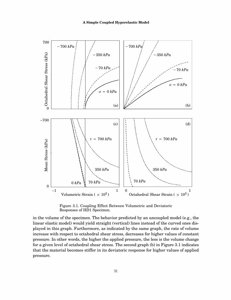
Figure 3.1 displays the results of a numerical experiment in which octahedral shearstress � is applied to the specimen under various values of constant (compressive) pres-sure (i.e., 0, –70, –350, –700 kPa or 0, –10, –50, –100 psi, respectively) for the HD1 mate-rial parameter values described in the next Chapter. The first graph (a) on Figure 3.1shows the variation of volumetric strain � with respect to octahedral shear stress. As indi-cated by this graph, purely deviatoric loading (i.e., octahedral shear) causes an increase
A Simple Coupled Hyperelastic Model
31
Figure 3.1. Coupling Effect Between Volumetric and DeviatoricResponses of HD1 Specimen.
Oct
ahed
ral S
hear
Str
ess
(kP
a)
0
700
Volumetric Strain ( � 102 ) Octahedral Shear Strain ( � 102 )
Mea
n St
ress
(kP
a)
0
–700
–1 1 0 1
�700 kPa
�350 kPa
�70 kPa
� � 0 kPa
�350 kPa
�70 kPa
� � 700 kPa
350 kPa
70 kPa0 kPa
� � 700 kPa
350 kPa
70 kPa
(a) (b)
(c) (d)
�700 kPa
� � 0 kPa
in the volume of the specimen. The behavior predicted by an uncoupled model (e.g., thelinear elastic model) would yield straight (vertical) lines instead of the curved ones dis-played in this graph. Furthermore, as indicated by the same graph, the rate of volumeincrease with respect to octahedral shear stress, decreases for higher values of constantpressure. In other words, the higher the applied pressure, the less is the volume changefor a given level of octahedral shear stress. The second graph (b) in Figure 3.1 indicatesthat the material becomes stiffer in its deviatoric response for higher values of appliedpressure.

Chapter 3
32
The results of the dual experiment to the one described above in which pressure � isapplied to the specimen under various values of constant octahedral shear stress (i.e., 0,70, 350, 700 kPa) is displayed again in Figure 3.1. Graphs (c) and (d) indicate that as thepressure is decreased from –700 kPa to 0 kPa (–100 psi to 0 psi), material becomes lessstiff in its deviatoric response and may eventually fail for low values of hydrostatic pres-sure.
3.3 Limiting the Tensile ResistanceThe stresses in a particulate medium are transferred through contact and friction be-tween the grains. Therefore, when there is no confinement, granular materials have nomeans of transferring the forces between the grains. Confinement can be quantified byusing the volumetric stress (hydrostatic pressure) or volumetric strain as a measure. In-tuitively, granular materials should have no capacity to bear tensile hydrostatic loading.This phenomenon can be approximated within the context of hyperelasticity.
3.3.1 A Multiplicative Modification to the Strain Energy Density Function (MD)
To limit the tensile response we modify the strain energy function by multiplying an addi-tional term p(�) with the original strain energy density function that will limit the meantensile stress when � � 0. Thus, the modified strain energy density is defined as
��(�, �) � �(�, �)p(�) (3.10)
where �(�, �) is the strain energy given by Eqn. (3.5) and p(�) is yet to be determined. Themodified stress is given by the derivative of the modified strain energy density with re-spect to the strain as
S� � �K�–3c�2�p(�) ��(�, �)p�(�)I � 2G � 2b�2 � 2c��p(�)E (3.11)
The modified mean stress and octahedral stress are, therefore, given by
�� � K�� 3c�2�p(�) ��(�, �)p�(�)
�� � 2G�� 2b�3 � 2c���p(�)
(3.12)
We shall construct the function p so that the modified mean stress �� and octahedralshear stress �� decay as the tensile volumetric strain increases, i.e. � � ��. Keeping thisin mind, let us define a family of functions,
qn(�) � 1 � (1 � e–a�)n (3.13)
that depend upon the volumetric strain � and proceed asymptotically to zero for all valuesof n. The constant a controls the rate at which the functions qn(�) ramp down. Note thatthe first and second derivatives of qn(�) are given by,

A Simple Coupled Hyperelastic Model
33
qn�(�) � �n�e–a�(1 � e–a�)n�1
qn��(�) � �n�2e–a�(1 � ne–a�)(1 � e–a�)n�2
(3.14)
Let us denote, for � � 0, the mean stress and octahedral stress given by Eqn. (3.7) as
�– � K�–3c�2�
�– � 2G�� 2b�3–2c���
(3.15)
Thus, upon comparing Eqns. (3.12) and (3.15), we see that, to enforce the continuity ofstresses and –as we shall see later– the continuity of the material tangent stiffness at� � 0, the function p(�) has to satisfy,
p(0) � 1, p�(0) � p��(0) � 0 (3.16)
Note that, the function qn(�) satisfies these same conditions for n 3. Since for � � 0, theterm 1 � e��� � 1, we see that among the family of functions qn(�), the function q3(�) is thefastest decaying one for a given �. Thus we may choose,
p(�) � q3(�) (3.17)
so that ��(0, �) � �–(0, �) and ��(0, �) � �
–(0, �). Also note that the continuity requirements��(0, 0) � �
–(0, 0) and ��(0, 0) � �–(0, 0) are satisfied automatically.
As Eqn. (3.12) indicates, the parameter a controls the rate of decay of stresses underpositive volumetric strain. Since the rate of decay cannot be determined from experimentone can simply choose it to be sufficiently large. This parameter can be interpreted as apenalty parameter: the larger the value of this parameter, the less is the resistance of thematerial to tension and shear. As one may anticipate, for extremely large values of a,one may suffer numerical difficulties because the material tangent stiffness has to takea sharp turn around where � � 0. As we shall see in the following sections, this value ofa can typically be chosen in the range of 103–105 which is appropriate for very fast decayof the response with positive volumetric strain.
The strain energy density is therefore given by different equations in compression andtension, which we will designate as
�M(�, �) ��(�, �)�(�, �)p(�)
� � 0� � 0
(3.18)
We shall refer to this formulation as coupled hyperelastic model with multiplicative decayor MD for short for the remainder of this study.
3.3.2 An Additive Modification to the Strain Energy Density Function (AD)Similarly, to limit the tensile response we can modify the strain energy function by ad-ding an additional term h(�, �) that will limit the mean tensile stress when � � 0. Themodified strain energy density is defined as

Chapter 3
34
��(�, �) � �(�, �) � h(�, �) (3.19)
where �(�, �) is the strain energy given by Eqn. (3.5) and h(�, �) is yet to be determined.The modified stress is given by the derivative of the modified strain energy density withrespect to the strain as
S� � K�� 3c�2 ��h��I � 2G � 2b�2 � 2c�� 1
3��h��E (3.20)
The modified mean stress and octahedral stress are, therefore, given by
�� � K�� 3c�2 ��h
��
�� � 2G�� 2b�3 � 2c��� 1
3�h��
(3.21)
We shall construct the function h so that the modified mean stress �� approaches aconstant limiting value �o as the tensile volumetric strain increases. The transition fromcompressive to limiting tensile response can be accomplished by ramping up the constantterm �o and ramping down the term K��3c�2 with complementary sigmoid functions as
�� � �o[1�d0(�)] � �K��3c�2�d0(�) (3.22)
where d0(�) is the zeroth member of the family of functions
dn(�) � 1(2a)n
�4n � (2n � e–a�)2� (3.23)
that depend upon the volumetric strain � and proceed asymptotically to zero for all valuesof n. The constant a controls the rate at which the functions dn(�) ramp down. Note thatthis family of functions has the special property
dn� � �dn–1 (3.24)
Let us assume, for the moment, that � � 0, thus, comparing Eqn. (3.22) with Eqn. (3.12)we find that
�h�� � �o � K�� 3c�2[1�d0(�)] (3.25)
If we integrate Eqn. (3.16) with respect to � we get
h(�, �) � �o � 3c�2[�� d1(�)] � K�12 �2 � �d1(�) � d2(�)� � k(�) (3.26)
where k(�) denotes the integration constant. The veracity of Eqn. (3.17) is easily verifiedby differentiation, noting the property given by Eqn. (3.24). We can now compute
�h�� � 6c�[�� d1(�)] � k�(�) (3.27)

A Simple Coupled Hyperelastic Model
35
The octahedral shear stress, when � � 0 is given by Eqns. (3.12) and (3.27) as
�� � 2G� � 2b�3 � 2c�d1(�) � 1
3 k�(�) (3.28)
There is some flexibility in determining the function k(�). The third term vanishes as� ��. Since the function d1(�) is not zero at � � 0, the term 2c�d1(�) causes a jump inthe shear modulus at � � 0. To assure the continuity of octahedral shear stress, theconstant has to be
k(�) � ko � c�2d1(0) (3.29)
where the value of ko is immaterial and can be taken as zero and d1(0) � 32a. This choiceof the function k(�) results in the expression
�� � �2G � 2b�2 � 2c(d1(0)�d1(�))�� (3.30)
The shear stress is nonlinear in the shear deformation � with initial stiffness (2G � 2b�2)decaying to a final stiffness of 2G � 2b�2�2cd1(0). Since d1(0) � 32a, ignoring for the mo-ment, the higher order term 2b�2, we must have
G � 3c2a (3.31)
Since the rate of decay cannot be determined from experiment one can simply choose itagain to be sufficiently large while satisfying Eqn. (3.31). As we shall see in the followingsection, this value of a can typically be chosen within the range of 103–105, which is ap-propriate for very fast decay of the response with positive volumetric strain. Note thatfor very large values of the parameter a the shear response of the material becomes un-coupled from the volumetric response. The final form of the constitutive relationship for� � 0 can be written as
S� � ��o(1�d0(�)) � K��3c�2�d0(�)�I � �2G � 2b�2 –2c(d1(0)�d1(�))�E (3.32)
where dn(�) is given by Eqn. (3.13). As we shall demonstrate later, this modification limitsthe pressure while allowing for the granular medium to dilate under deviatoric loading.Note that the continuity requirements for the stress, i.e. �
�(0, �) � �–(0, �) and
��(0, �) � �
–(0, �) are satisfied. Also note that the continuity requirements at zero strain��(0, 0) � �
–(0, 0) and ��(0, 0) � �–(0, 0) are satisfied as well.
The strain energy density is therefore given by different equations in compression andtension, which we will designate as
�A(�, �) ��(�, �)�(�, �) � h(�)
� � 0� � 0
(3.33)
We shall refer to this formulation as coupled hyperelastic model with additive decay orAD for short for the remainder of this study.

Chapter 3
36
Figure 3.2. Response of HD1 for original and additive decay (AD) modelsunder prescribed strains.
Oct
. She
ar S
tres
s (m
Pa)
0
1.75
0 2.5Octahedral Shear Strain ( � 102 )
Mea
n St
ress
(kP
a)
–700
700
–2 2Volumetric Strain ( � 102 )
AD model
originalmodel
70
Remark. Eqn. (3.30) implies that the octahedral shear stress grows with octahedralshear strain, independent of the volumetric strain. This artifact is undesirable, however,for very large values of the parameter a, the shear stiffness of the material under positivevolumetric strain will be considerably less than its response under compression. Keepingin mind that both modifications (AD and MD) are merely attempts to assess the materialbehavior close to failure, and the actual behavior of the material under positive volumet-ric straining can not properly be characterized without the consideration of plastic de-formations, we shall nevertheless proceed with the AD formulation, treating it as a sim-ple approximation of the response of the material near failure.
3.3.3 A Numerical ExperimentIn order to display the behavior the constitutive models presented earlier in this chapter(i.e. original model, model with additive decay (AD) and model with multiplicative decay(MD)), we shall conduct a numerical experiment. In this experiment a single materialpoint is proportionally loaded with a prescribed volumetric and octahedral shear strains. Thematerial constants are those of the granular material designated as HD1 by Allen (1973)(see Chapter 4).
Figure 3.2 displays the results for the original formulation and the AD model. Arrowsin the figure indicate the direction of loading. For the AD model, the additional materialconstants were chosen as �o � 70 kPa (or 10 psi) and � � 5000. As expected, for the AD
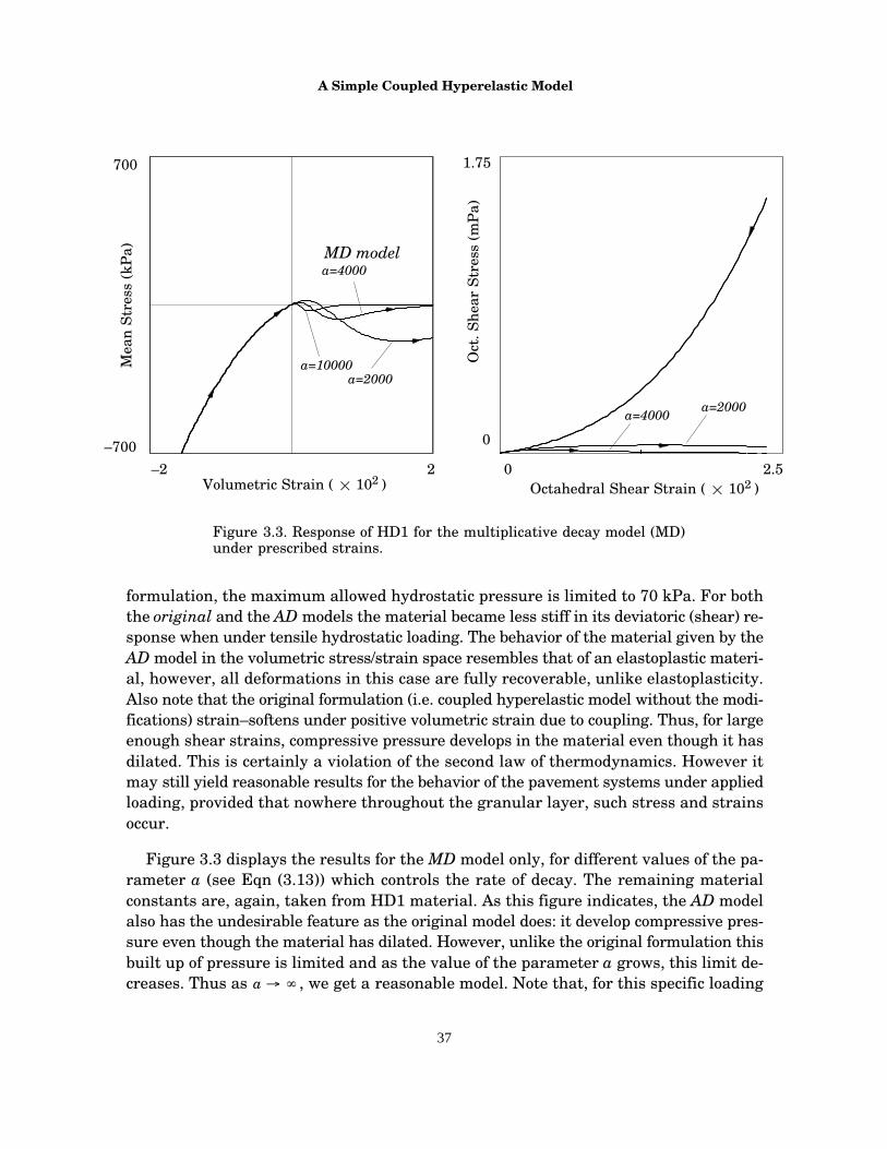
A Simple Coupled Hyperelastic Model
37
Oct
. She
ar S
tres
s (m
Pa)
0
1.75
0 2.5Octahedral Shear Strain ( � 102 )
Figure 3.3. Response of HD1 for the multiplicative decay model (MD)under prescribed strains.
Mea
n St
ress
(kP
a)
–700
700
–2 2Volumetric Strain ( � 102 )
a=4000
a=2000a=10000
MD model
a=2000a=4000
formulation, the maximum allowed hydrostatic pressure is limited to 70 kPa. For boththe original and the AD models the material became less stiff in its deviatoric (shear) re-sponse when under tensile hydrostatic loading. The behavior of the material given by theAD model in the volumetric stress/strain space resembles that of an elastoplastic materi-al, however, all deformations in this case are fully recoverable, unlike elastoplasticity.Also note that the original formulation (i.e. coupled hyperelastic model without the modi-fications) strain–softens under positive volumetric strain due to coupling. Thus, for largeenough shear strains, compressive pressure develops in the material even though it hasdilated. This is certainly a violation of the second law of thermodynamics. However itmay still yield reasonable results for the behavior of the pavement systems under appliedloading, provided that nowhere throughout the granular layer, such stress and strainsoccur.
Figure 3.3 displays the results for the MD model only, for different values of the pa-rameter a (see Eqn (3.13)) which controls the rate of decay. The remaining materialconstants are, again, taken from HD1 material. As this figure indicates, the AD modelalso has the undesirable feature as the original model does: it develop compressive pres-sure even though the material has dilated. However, unlike the original formulation thisbuilt up of pressure is limited and as the value of the parameter a grows, this limit de-creases. Thus as a � �, we get a reasonable model. Note that, for this specific loading
Chapter 3
38
a � 4000 yields a reasonable response for the behavior of the HD1 material under posi-tive volumetric strains.
3.4 Material Tangent StiffnessTo perform numerical computations with nonlinear material models one must evaluatethe material tangent stiffness �. The material tangent stiffness � for the proposed modelcan easily be computed as
� � �S�E (3.34)
The stress is given by different equations in compression and tension, which we will des-ignate as
S �S�
S�
� � 0� � 0
(3.35)
where the tensor S� is given by Eqn. (3.6) for all of the models discussed in this chapter.For the original coupled model S� is the same as S�. For the coupled model with multipli-cative decay (MD), S� is given by Eqn. (3.11) and for the coupled model with additivedecay (AD) S� is given by Eqn. (3.32). The material tangent stiffness � can also be ex-pressed as
� ��
�
��
� � 0� � 0
(3.36)
Material tangent stiffness tensor for the original model. From Eqn. (3.6) one can computethe material tangent modulus in compression to be
��(�, �) � KI � I � 2�G�b�2�c�1
� 2c�E � I � I � E� 2bE � E
(3.37)
This is also the material tangent stiffness tensor for the original model in tension.
Material tangent stiffness for the MD model. From Eqn. (3.11) one can compute the mate-rial tangent modulus in tension to be
��(�, �) � �Kq(�) � 2K�� 3c�2�q�(�) ��(�, �)q��(�)I � I
� �2G � 2b�2 –2c��q�(�) � 2cq(�)�E � I�I � E
� 43 bE � E � 2G � 2b�2 –2c��q(�)1
(3.38)
Material tangent stiffness for the AD model. From Eqn. (3.32) one can compute the mate-rial tangent modulus in tension to be
A Simple Coupled Hyperelastic Model
39
��(�, �) � �Kd0(�) � ��o�K��3c�2d–1(�)�I � I
� 2cdo(�)�E � I�I � E�� 43 bE � E
� �2G � 2b�2 –2c(d1(0)�d1(�))�1
(3.39)
where I � I is the fourth order identity tensor with components [I � I]ijkl � �ij�kl, 1 is thefourth order tensor with components 1ijkl � �ik�jl�
13 �ij�kl, and the components of the ten-
sor I � E are �I � E�ijkl
� �ijEkl. The functions dn(�) are given by Eqn. (3.23). One can seethat the tangents for all the models satisfy the continuity relationships
��(0, �) � �
–(0, �), ��(0, 0) � �
–(0, 0) (3.40)
Also note that the material tangent stiffness for all the models at zero strain is
�(�, �) � KI � I � 2G1 (3.41)
3.5 Plate Loading TestThe constitutive models described earlier are implemented to a finite element analysiscode (ABAQUS, 1994) and a plate loading test is performed. The circular plate which is20.3 cm. (8 inches) thick and has a radius of 380 cm. (150 inches) is made of asphalt con-crete. It is loaded with a distributed load of 700 kPa (100 psi) with a radius of 24.6 cm.(9.7 inches). In addition to the wheel load, gravity loads (i.e. self weight of the structure)are include in the analyses. The plate stands on top of a 76.2 cm. (30 inches) thick layerof HD1 material. The bottom layer is natural soil. The lateral and vertical extent of thefinite element model are chosen to be 40 times the radius of the wheel load, sufficientlyremote so that the stresses and strains of interest (i.e. values within the vicinity of theload) are not significantly effected by the remote boundary conditions. The boundaryconditions at the remote vertical boundary were chosen such that the displacements inthe vertical (z) direction were fixed. The geometry and the axisymmetric finite elementmesh are displayed on Figure 3.4.
The densities of the materials were taken to be 0.0024 kgf�cm3 for the (asphalt cons-rete) plate, 0.0022 kgf�cm3 for the crushed rock, and 0.0017 kgf�cm3 for the natural soil.The plate was assumed to be linearly elastic with Young’s modulus E�2070 MPa (300ksi) and Poisson’s ratio of � � 0.15. The natural soil was also assumed to be linearly elas-tic with Young’s modulus E�40 MPa (6 ksi) and Poisson’s ratio of � � 0.45. The secondlayer was modeled using one of the following four models: (a) linear elasticity withE�240 MPa (34.9 ksi) and � � 0.34, (b) original model with K�166 MPa (24 ksi),G�52.4 MPa (7.6 ksi), b�3.2�107 MPa (4.63�109 ksi) and�c�4.3�104 MPa (6.3�103
ksi)� (c) AD model with all material constants same as the original model with its addi-tional constants a=5000 and �o � 0 MPa.and finally (d) MD model, again with all materi-al constants same as the original model and with its additional constant a�4000. Thevalues of these material constants are for the high density crushed rock material desig-nated as HD1 by Allen (1973) (see Chapter 4).
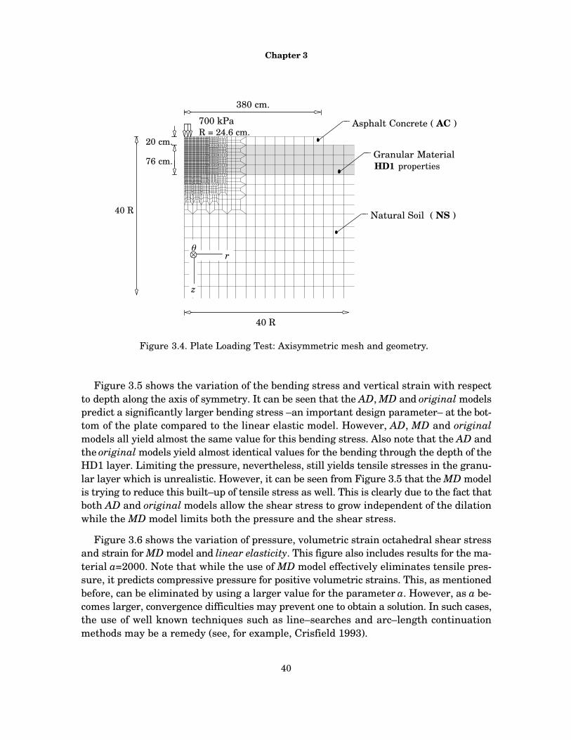
Chapter 3
40
Figure 3.4. Plate Loading Test: Axisymmetric mesh and geometry.
R = 24.6 cm.20 cm.
76 cm.
40 R
Asphalt Concrete
Granular Material
Natural Soil
HD1 properties
700 kPa ( AC )
( NS )
380 cm.
40 R
z
r�
Figure 3.5 shows the variation of the bending stress and vertical strain with respectto depth along the axis of symmetry. It can be seen that the AD, MD and original modelspredict a significantly larger bending stress –an important design parameter– at the bot-tom of the plate compared to the linear elastic model. However, AD, MD and originalmodels all yield almost the same value for this bending stress. Also note that the AD andthe original models yield almost identical values for the bending through the depth of theHD1 layer. Limiting the pressure, nevertheless, still yields tensile stresses in the granu-lar layer which is unrealistic. However, it can be seen from Figure 3.5 that the MD modelis trying to reduce this built–up of tensile stress as well. This is clearly due to the fact thatboth AD and original models allow the shear stress to grow independent of the dilationwhile the MD model limits both the pressure and the shear stress.
Figure 3.6 shows the variation of pressure, volumetric strain octahedral shear stressand strain for MD model and linear elasticity. This figure also includes results for the ma-terial a=2000. Note that while the use of MD model effectively eliminates tensile pres-sure, it predicts compressive pressure for positive volumetric strains. This, as mentionedbefore, can be eliminated by using a larger value for the parameter a. However, as a be-comes larger, convergence difficulties may prevent one to obtain a solution. In such cases,the use of well known techniques such as line–searches and arc–length continuationmethods may be a remedy (see, for example, Crisfield 1993).
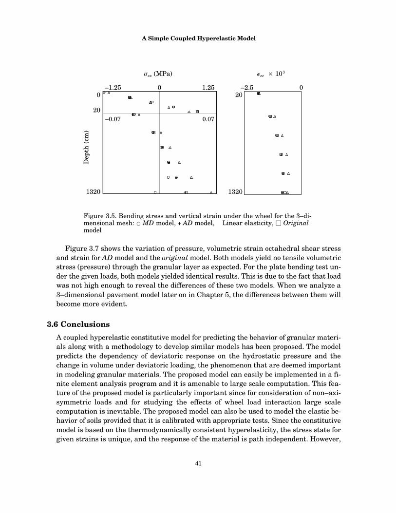
A Simple Coupled Hyperelastic Model
41
Figure 3.5. Bending stress and vertical strain under the wheel for the 3–di-mensional mesh: � MD model, + AD model, � Linear elasticity, � Originalmodel
–1.25 1.25
20
0
1320
Dep
th (
cm)
–0.07 0.07
–2.50 0
�xx (MPa) �zz � 103
20
1320
Figure 3.7 shows the variation of pressure, volumetric strain octahedral shear stressand strain for AD model and the original model. Both models yield no tensile volumetricstress (pressure) through the granular layer as expected. For the plate bending test un-der the given loads, both models yielded identical results. This is due to the fact that loadwas not high enough to reveal the differences of these two models. When we analyze a3–dimensional pavement model later on in Chapter 5, the differences between them willbecome more evident.
3.6 ConclusionsA coupled hyperelastic constitutive model for predicting the behavior of granular materi-als along with a methodology to develop similar models has been proposed. The modelpredicts the dependency of deviatoric response on the hydrostatic pressure and thechange in volume under deviatoric loading, the phenomenon that are deemed importantin modeling granular materials. The proposed model can easily be implemented in a fi-nite element analysis program and it is amenable to large scale computation. This fea-ture of the proposed model is particularly important since for consideration of non–axi-symmetric loads and for studying the effects of wheel load interaction large scalecomputation is inevitable. The proposed model can also be used to model the elastic be-havior of soils provided that it is calibrated with appropriate tests. Since the constitutivemodel is based on the thermodynamically consistent hyperelasticity, the stress state forgiven strains is unique, and the response of the material is path independent. However,

Chapter 3
42
Figure 3.6. Variation of volumetric and octahedral shear stressand strain through depth for MD model and linear elasticity.
Dep
th (
cm.)
96
20
a=4000
a=2000MD model
a=4000
linear elastic
–150 150 –5 5
a=2000linear elastic
0 10 150
� (kPa)
� (kPa)
� (� 104)
� (� 103)
Dep
th (
cm.)
96
20
a=4000
a=2000
linear elasticity
a=4000
a=2000MD model
linear elastic
the bounds on the material constants within which the constitutive model is stable andunique are not established.
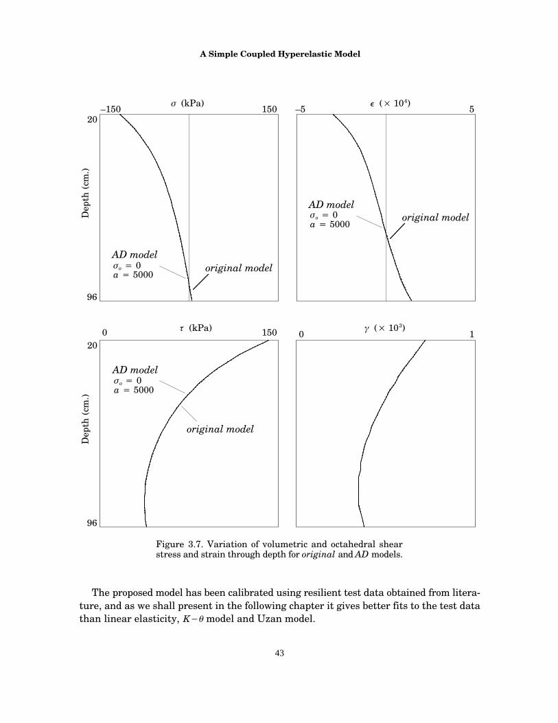
A Simple Coupled Hyperelastic Model
43
Figure 3.7. Variation of volumetric and octahedral shearstress and strain through depth for original and AD models.
Dep
th (
cm.)
96
20
AD modeloriginal model
–150 150 –5 5
0 10 150
� (kPa)
� (kPa)
� (� 104)
� (� 103)
Dep
th (
cm.)
96
20
�o � 0a � 5000
AD modeloriginal model�o � 0
a � 5000
AD model
original model
�o � 0a � 5000
The proposed model has been calibrated using resilient test data obtained from litera-ture, and as we shall present in the following chapter it gives better fits to the test datathan linear elasticity, K�� model and Uzan model.
Chapter 3
44
The fact that the granular materials have no or little tensile stress bearing capabilityhas important implications to the design of pavement systems. To this end, we have pro-posed two alternative modifications to the original coupled hyperelastic model which ef-fectively allows the control of the maximum hydrostatic tensile stress value and the waythe tension-limited state is achieved can easily be manipulated and changed by using dif-ferent forms of the auxiliary energy density functions, p(�, �) for the model with additivedecay (AD) and q(�) for the model with multiplicative decay (MD).

45
Chapter 4
Determination of Material Constants
Determination of material constants from experimental data is an important part ofconstitutive modelling. This chapter deals with the calibration of the K– � , Uzan–Witzcakmodels and the coupled hyperelastic model (i.e. the original model) described in Chapter3 from experimental data. Experimental data is obtained from available literature andstatistical comparison of the success of K– � , Uzan–Witzcak , coupled model and LinearElasticity models in predicting the experimental values is presented.
4.1 Experimental DataThe resilient triaxial test data was obtained by Allen and Thompson at the Universityof Illinois (1973). They conducted tests on nine different specimens, and measured bothvertical and lateral strains during each test. A brief description of these materials areshown in Table 4.1.
Specimen Material Density, kg/m3
2240217021102260
21252170
226021802125
HighIntermediateLowHighIntermediateLowHighIntermediateLow
HD1MD1LD1HD2MD2LD2HD3MD3LD3
Crushed StoneCrushed StoneCrushed Stone
GravelGravelGravelBlendBlendBlend
Note: 1 kg/m3 � 0.0617 lbs/ft3
Table 4.1. Test Specimens of Allen–Thompson Resilient Tests (Allen 1973).
The samples were first subjected to several cycles of certain stress patterns to achieveresilient behavior (i.e. shakedown). This phase is called preconditioning. Preconditioningsimulates the actual response of granular layers in pavements at very early stages oftheir service life. Allen and Thompson report that after 10 to 20 cycles the samples were
Determination of Material Constants
46
almost entirely shaken down and the response after this stage was essentially nonlinearelastic. The samples were then subjected to repeated stress pulses with levels anticipatedin granular layers of pavements under wheel loads. The data set of these experimentscan be found in Appendix III.
4.2 A Weighted Nonlinear Least Squares ProcedureThe values of the material constants were determined through a weighted nonlinearleast squares curve fitting procedure. In a triaxial test the axial stress �1 and the lateralstress �2 are measured. From these measured values the mean and octahedral stressescan be computed as
� � 13
(�1�2�2), � � 2�
3(�1 � �2) (4.1)
The axial strain �1 and lateral strain �2, are also measured. From these measured valuesthe mean and octahedral strains can be computed as
� � (�1�2�2), � � 2�
3(�1 � �2) (4.2)
Let us define the mean and deviatoric residual functions as,
r i(x) � �^i � �i(x, �̂i, �^i), si(x) � �^i � �i(x, �̂i, �^i) (4.3)
where {�^i, �^i, �̂i, �^i} are the measured stresses and strains for observation i and for thecoupled hyperelastic model described in Chapter 3, for example, x�{K, G, b, c} is the vec-tor of unknown material constants. To determine the constitutive parameters from triax-ial measurements we minimize the weighted least-squares residual function
g(x) � 12 ��N
i�1
r2i (x) � (1��)�
N
i�1
s2i (x)� (4.4)
where the weight parameter � can be specified to have a value between 0 and 1. By vary-ing the value of � we can apply different weights to the volumetric and deviatoric compo-nents of the test data. This is done to take into account the relative difference in the mag-nitudes of the volumetric and deviatoric stress and strain, with the hope of obtaining abetter fit for values of � other than 0.5.
The gradient and the Hessian of the objective function are given by,
�g(x) � �JTmr � (1��)JT
ds
Hg(x) � �JTmJm � (1��)JT
dJd
(4.5)
respectively. The ij th components of the Jacobian matrices are computed with the follow-ing convention [Jm]ij � �r i��xj and Jd
ij � �s i��xj. Beginning with an initial guess x(o) one
can generate a sequence of approximations �x(k)� according to the recursion formula
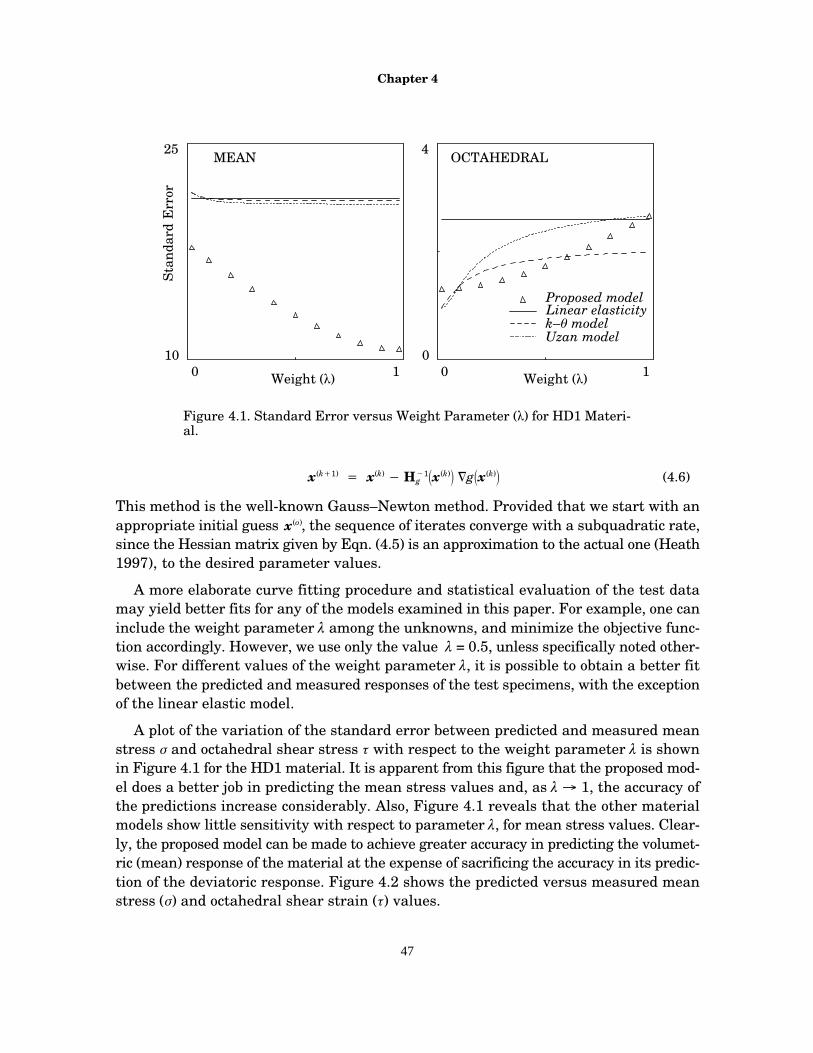
Chapter 4
47
Stan
dard
Err
or
10
25
0 10
4
0 1
Figure 4.1. Standard Error versus Weight Parameter (�) for HD1 Materi-al.
OCTAHEDRALMEAN
k–� modelLinear elasticity
Uzan model
Proposed model
Weight (�) Weight (�)
x(k�1) � x(k) � H�1g �x(k)� �g�x(k)� (4.6)
This method is the well-known Gauss–Newton method. Provided that we start with anappropriate initial guess x(o), the sequence of iterates converge with a subquadratic rate,since the Hessian matrix given by Eqn. (4.5) is an approximation to the actual one (Heath1997), to the desired parameter values.
A more elaborate curve fitting procedure and statistical evaluation of the test datamay yield better fits for any of the models examined in this paper. For example, one caninclude the weight parameter � among the unknowns, and minimize the objective func-tion accordingly. However, we use only the value � = 0.5, unless specifically noted other-wise. For different values of the weight parameter �, it is possible to obtain a better fitbetween the predicted and measured responses of the test specimens, with the exceptionof the linear elastic model.
A plot of the variation of the standard error between predicted and measured meanstress � and octahedral shear stress � with respect to the weight parameter � is shownin Figure 4.1 for the HD1 material. It is apparent from this figure that the proposed mod-el does a better job in predicting the mean stress values and, as � � 1, the accuracy ofthe predictions increase considerably. Also, Figure 4.1 reveals that the other materialmodels show little sensitivity with respect to parameter �, for mean stress values. Clear-ly, the proposed model can be made to achieve greater accuracy in predicting the volumet-ric (mean) response of the material at the expense of sacrificing the accuracy in its predic-tion of the deviatoric response. Figure 4.2 shows the predicted versus measured meanstress (�) and octahedral shear strain (�) values.

Determination of Material Constants
48
Linear ElasticityP
redi
cted
(kP
a)
Measured (kPa)
Figure 4.2. Predicted vs. Measured Response of HD1 Specimen(Test Allen, Thompson 1976).
Measured (kPa)
OCT.MEAN
–70
275
–70
275
–70 275 –70 275
K–� Model
Uzan–Witzcak Model Coupled Hyperelastic Model
Pre
dict
ed (
kPa)
Figure 4.3 shows the distribution of standard error between the predicted and mea-sured values of volumetric and octahedral shear stress values for all the specimens. Asthis figure indicates, the proposed coupled hyperelastic model generally did better thanthe other three models in predicting the measured volumetric and octahedral stress val-ues. The total success of any of these constitutive models is a combination of their predic-tions in volumetric and octahedral stress spaces. A brief investigation of the test data re-veals that, the magnitude of the octahedral stresses and strains in all of the tests were

Chapter 4
49
Figure 4.3. Distribution of Standard Error Between Predictedand Measured Stress Values for Various Material Models.
������
���
���������
������
���
���������
������
���������
������
���������
���������
������
��������
���������
���������
���������
50
0
5
0
HD1 HD2 HD3 MD1 MD2 MD3 LD3LD2LD1
HD1 HD2 HD3 MD1 MD2 MD3 LD3LD2LD1
Octahedral
Mean��
k–� model
Linear elasticity Uzan model
Proposed model
relatively smaller than the volumetric stress and strain values. As these measurementswere probably made with similar instruments, the octahedral measurements would bemore polluted by experimental error. Therefore, one can intuit that the data fit for thevolumetric response would be better. The values in Figure 4.3 were computed for � = 0.5.However, for each specimen, there always was a value of � such that the standard errorof both the predicted mean and octahedral stress values were less for the proposed model,than for the other models. For example, the range of � for the HD1 specimen for whichthe proposed model always does better is between 0.1 and 0.6.
Remark. In most cyclic triaxial tests the lateral strain �2 is not measured. The evalua-tion of the material parameters goes as follows. The resilient modulus Mr is measuredfor each level of applied stress and tabulated as the ratio (�1��2)��1. The materialconstants k, n, and m (of the Uzan-Witzcak model) are determined by minimizing the er-ror function e(k, n, m) � ln(Mmeas
r ) � ln(k�n�
m), where Mmeasr is the value of the measured ra-
tio (�1��2)��1 and � � 13 |�1�2�2| and � � 2� |�1��2|�3 are evaluated from the measured
applied stresses. This data fit can be done with linear least-squares. Unfortunately, thevalues of the material constants obtained by this procedure are not consistent with theconstitutive model described by Eqn. (2.18). In fact, it is impossible to uniquely assessthe material constants from triaxial test data without the lateral strain �2. Throughoutthis manuscript, when we refer to the K–� or Uzan-Witzcak models we mean the model
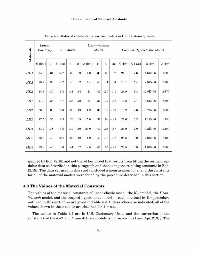
Determination of Material Constants
50
Table 4.2. Material constants for various models in U.S. Customary units.
Linear
E (ksi) � k (ksi) b (ksi) c (ksi)G (ksi)� n k (ksi) � n m K (ksi)
ElasticityUzan–Witzcak
Model
HD1
HD2
HD3
LD1
LD2
LD3
MD1
MD2
MD3
Mat
eria
ls
34.9
28.2
44.6
31.0
26.0
27.5
33.9
28.8
29.8
.34
.38
.40
.36
.36
.36
.38
.40
.40
14.2 .33 .29 14.8 .33 .22 .07
2.2 .43 .82
6.3 .41 .64
.36 .70
.36 .49
.36 .39
.69.39
.29 .40
.41 .67
3.7
6.0
8.3
3.8
13.7
3.6
.43
.42
.36
.35
.36
.40
.41
.40
.41
2.0
1.2
1.2
.63
–.25
.78
.95
.34
–1.1
–.38
–.59
–.23
.67
–.37
–.27
4.4
.41
1.9
.54
5.9
24.0
4.9
2.5
K–� Model
24.1 7.6
18.1 5.4
26.9 6.4
16.8 2.7
16.2 2.6
21.6 6.3
24.9 2.0
28.6 6.0
29.5 6.8
8900
6200
16870
8600
6600
4250
11200
5100
5800
4.6E+06
2.8E+06
12.0E+06
5.5E+06
3.7E+06
1.1E+06
9.2E+06
2.0E+06
1.8E+06
Coupled Hyperelastic Model
implied by Eqn. (2.18) and not the ad hoc model that results from fitting the resilient mo-dulus data as described in this paragraph and then using the resulting constants in Eqn.(2.18). The data set used in this study included a measurement of �2 and the constantsfor all of the material models were found by the procedure described in this section.
4.3 The Values of the Material Constants
The values of the material constants of linear elastic model, the K–� model, the Uzan-Witzcak model, and the coupled hyperelastic model — each obtained by the procedureoutlined in this section — are given in Table 4.2. Unless otherwise indicated, all of thevalues shown in these tables are obtained for � � 0.5.
The values in Table 4.2 are in U.S. Customary Units and the conversion of theconstant k of the K–� and Uzan-Witzcak models is not so obvious ( see Eqn. (2.3) ). The

Chapter 4
51
value of k in SI units (kPa) can be computed by multiplying its value in U.S. CustomaryUnits (psi) by 6.895(1�n�m).
4.4 ConclusionsAs the results indicate, the coupled hyper elastic model described in Chapter 3 does a bet-ter job in predicting the measured stress values than the K– � and Uzan–Witzcak models.Furthermore, it is observed that the coupled hyperelastic model displays a welcome sen-sitivity to the weight parameter � of the nonlinear least squares procedure unlike theother models described earlier. Using this parameter, one can take into account the pos-sible differences of the accuracy of the volumetric and deviatoric strain measurementsif desired. The fact that the coupled model yields a better fit to the test data using samenumber material constants (four) as the Uzan–Witzcak model indicates that the simpleidea of coupling the volumetric deviatoric responses of the material within the contextof hyperelasticity is indeed a fruitful one. This coupling is also present in both the K– �and Uzan–Witzcak models, yet in a more subtle way. Nevertheless, the coupled hyper-elastic model somehow makes a better use of the flexibility provided by the four constantsit uses. It also provides a welcome feature that one can interpret the meanings of theseconstants much more directly.
52
Chapter 5
A Projection Operator for No−Tension Elasticity
In this chapter a tensor–valued projection operator which operates on the stress tensoris proposed where the projected stress has principal values that are less than or equalto a preassigned value. Such a projection yields constitutive laws for materials with lim-ited tensile/compressive strength. These constitutive models can also be viewed as de-formation plasticity models in principal directions. Applications of the proposed class ofconstitutive models include stability and limit load analysis of structures such as tunnelsor excavations into rock mass, masonry walls and pavements with compacted layers ofgranular materials which is the subject of this study. Researchers in the past have ap-proached such problems using numerical (Zienkiewicz et. al, 1968) and analytic (DelPiero, 1989) methods and using elastic–perfectly plastic models that utilize well–knownyield criteria such as Mohr–Coulomb all of which have fundamental differences with theproposed models.
The stress–update formulation and the derivation of the consistent tangent operatorfor the proposed models are provided for the finite element method. A robust implementa-tion requires the derivatives of the projection operator with respect to strain to obtain thematerial tangent stiffness. The non–uniqueness of the spectral form of the projection op-erator in the case of coalescence of the principal values creates a fundamental difficulty.Aforementioned derivatives are obtained with careful consideration of the limit cases(Carlson, 1986) of the well known formulas for distinct principal values (Kato, 1976). Aversion of the proposed model with linear elastic behavior under compression and limitbehavior under tension is implemented to a commercial finite element package (ABA-QUS, 1994). Quadratic convergence rate of the Newton–Raphson solution method withthis model for all possible cases (i.e. distinct, double and triple coalescence of principalvalues) is demonstrated with a few boundary value problems.
5.1 PreliminariesGiven the second–order symmetric tensor S : � � Sym(Vn)�, we can write, through thespectral decomposition of S,
S ��n
i�1
s iei(S) � ei(S) (5.1)
where {s1, s2,..., sn} is the spectrum of S and {e1(S), e2(S),..., en(S)} is an orthonormal basisof eigenvectors of S. The non–uniqueness of {ei(S)} in the representation above when S
� Vn denotes an n– dimensional normed vector space

Chapter 5
53
has repeated eigenvalues is an obstacle when the derivatives of S are needed in spectralform. An alternative representation theorem that has recently found its way into com-putational mechanics (Simo 1991, Schreyer 1993) is based on eigenprojections. To wit,
S �p
i�1
s iEi(S) (5.2)
where {s1, s2,..., sp} is the set of distinct eigenvalues of S and Ei(S) is the eigenprojectioncorresponding to s i. Unlike the basis {ei(S)}, the eigenprojections are unique and can beexpressed as (see, for example, Halmos 1958),
Ei(S) �
p
j�1j�i
S � s jIsi � sj
, p � 1,
I, p � 1,
(5.3)
where the integer p is the number of distinct eigenvalues of S. It can be shown that theeigenprojections have the following properties
Ei(S)Ej(S) �Ei(S), i � j,0, i � j, (5.4)
p
i�1
Ei(S) � I (5.5)
Since we are concerned with the stress tensor, we will restrict our attention to 3–di-mensional space (i.e. S : � � Sym(V3)), therefore p � 3. Let F : Sym(V3) � Sym(V3) be atensor–valued function defined as
F(S) �p
i�1
f(s i)Ei(S) (5.6)
where the function f : � � �, needs to be sufficiently smooth, as we shall see below, if thecontinuity and differentiability of F(S) is a requirement. Depending on the distinct eigen-values of S, we can equivalently state,
F(S) �
f(s1)E1(S) � f(s2)E2(S) � f(s3)E3(S), s1 � s2 � s3 � s1,
f(s1)E1(S) � f(s)[I�E1(S)], s1 � s2 � s3 � s ,
f(s)I, s1 � s2 � s3 � s .
(5.7)
In what follows, we present two essential theorems , the proofs of which are omittedfor brevity, due to Carlson and Hoger (Carlson 1986). Note that these theorems also holdfor functions f : � � � that are smoother than what is stated below.

No–Tension Elasticity
54
THEOREM. If f : � � �, is three times continuously differentiable, the functionF : Sym(V3) � Sym(V3) defined in Eqn. (5.7) is continuous.
THEOREM. If the function f, is seven times continuously differentiable on �, the func-tion F(S) is continuously differentiable on Sym(V3) and the derivative of F with respectto its argument is,
�(s1�s2)�3 � (s1�s3)�2 � (s2�s3)�1] 1, s1 � s2 � s3 � s1,�F(S)�S �
[�1 ��2 ��3] S2 � S2
�[s1s2�3 � s1s3�2 � s2s3�1] S2 � I � I � S2�
�(s1�s2)2�3 � (s1�s3)2�2 � (s2�s3)2�1 S � S
�[�1 � �2 � �3 � s1s2(s1�s2)�3 � s2s3(s2�s3)�1
�(s1s2)2�3 � (s1s3)2
�2 � (s2s3)2�1
�[(s1�s2)�3 � (s2�s3)�1 � (s1�s3)�2] S2 � S � S � S2�
�s1s3(s1�s3)�2] (S � I � I � S)
f�(s) 1, s1 � s2 � s3 � s,
1(s1�s)3
� [(s1�s)(f�(s1)�f�(s)) � 2(f(s1)�f(s))] S � S
�[(s1�s)(f(s1)�f(s)) � (s1�s)(sf�(s1)�s1f�(s))] (S � I � I � S)
�(s1�s)(s2f�(s1)�s21f�(s))
�2s1s(f(s1)�f(s))]1 �, s1 � s2 � s3 � s ,
(5.8)
where the scalars � i and �i are given by,
�i �1
(si�sj)2(si�sk)2
f�(si) � (si�s j)(� i��k) � (si�sk)(� i��j)
� i �f(s i)
(si�s j)(s i�sk)
(5.9)
with the indices i � j � k � i � {1, 2, 3}.
The non–commutative operation � in Eqn. (5.8) operates on two 2nd–order tensors andyields a 4th–order tensor, with components
Chapter 5
55
(A B)ijkl �12 (A ikBjl � AilBjk) (5.10)
When this product is contracted with another 2nd–order tensor it yields,
(A B) : X � ASym(X)B (5.11)
or in component form,
(A B)ijkl Xkl �12 Aik(Xkl � X lk)Blj (5.12)
where the summation convention is implied on repeated indices. Also, the 4th–orderidentity tensor 1 is,
1 ijkl� (I I)ijkl �12 (�ik�jl � �il�jk) (5.13)
Upon denoting � � F(S)�S, inspection of Eqn. (5.8) indicates that � possesses both ma-jor and minor symmetries
� ijkl � �klij � � jikl � � ijlk (5.14)
5.2 The Projection OperatorLet us define a function g : � � �,
g(s) � 12 [1 � tanh(�s)] (5.15)
where the scalar � ��. Note that the function is monotonic, that
lims���
g(s) � 1 and lims���
g(s) � 0 (5.16)
and that 0 � g(s) � 1 � s �. The function g(s), essentially a smooth switch function, isactually a specific form of the steady traveling wave solution for Burger’s equation thatdescribes the so–called Burger’s shock wave [see, for example, Jeffrey 1995].
Let us also define, a function f : � � �, such that
f(s) � � g(s)ds � s � 12�
ln�12 (e2�s � 1)�. (5.17)
Note that, the function f is infinitely many times differentiable on �. Taking the limit,
lims���
f(s) � 12�
ln(2) (5.18)
and defining smax � ln(2)�2�, we see that as s � ��, f(s) � s � smax. Using the definitionof smax we can rewrite Eqn. (5.15) as

No–Tension Elasticity
56
Figure 5.1. Effects of variation of scalar smax .
–1 10s
–0.5
1.5
g(s)
0
smax � 0.25
smax � 0.1
smax � 0.01
1.0
f�(s) � g(s) � 2s�smax � 1��1 (5.19)
The function g(s) is plotted in Figure 5.1 for various values of smax. We can see that, fromthis graph, the smaller is the constant smax, the steeper is the transition from left to right.Thus, we can control the shape of g(s) by changing the value of smax. Similarly, we canrewrite Eqn. (5.17) as
f(s) � s � smax
ln(2)ln[2g(s)] (5.20)
The variation of f, with respect to s is illustrated in Figure 5.2. Note that,
lims���
f(s) � smax. (5.21)
and f is bounded from above, i.e.,
f(s) � smax, � s �. (5.22)
With these in mind, let us define the no–tension projection operator F : Sym(V3) � Sym(V3)with (see Eqn. (5.7)),
F(S) � p
i�1
f(s i)Ei(S) (5.23)
where f : � � � is given by Eqn.’s (5.19) and (5.20). The function F(S) is continuous anddifferentiable due to the theorems stated earlier because f is infinitely many times differ-

Chapter 5
57
Figure 5.2. Function f.
–1 10s
f(s)
smax
–1
1
0
–1 10s
–1
1
0
f(s)
11
smax � 0.01smax � 0.25
smax
entiable. The derivative of F(S) with respect to its argument can simply be obtained fromEqns. (5.8) and (5.9). Note that, F(S) is symmetric by definition.
5.3 No–Tension ElasticityConsider a solid body � with boundary ��, having normal vector field n, subjected to ap-plied tractions t on ��t � �� and body forces b with prescribed displacements u on��u � ��, subject to, �� � ��u ��t and ��u ��t � �. Let S represent the stress tensorfield and E the strain tensor field in the interior of the body. The equations governing theresponse of the body constitute the boundary value problem (see, for example, Hjelmstad1997)
divS � b � 0 and ST � S
Sn � t
E � � (s)u � 12��u ��uT�
u � u
in �
in �
on ��t
on ��u
(5.24)
where the divergence is computed as [divS]i � �Sij��xj and the gradient as [�u]ij � �ui��xj.A superscript T indicates the transpose of the argument. To complete the statement ofthe boundary value problem we need only constitutive equations — the relationship be-tween S and E. Let us assume that the elastic response is characterized in terms of astrain energy density function W : Sym(V3) � � leading to a constitutive relation be-tween an intermediate stress state (Sh) and strain, i.e.,
Sh � �W(E). (5.25)

No–Tension Elasticity
58
Such a characterization is referred to as hyperelasticity (see, for example, Truesdell1965). To obtain a no tension material, we project the intermediate (hyperelastic) stress(Sh) with,
S � F(Sh) � F[W(E)] (5.26)
where, F : Sym(V3) � Sym(V3) is given by Eqn. (5.23). Thus Eqn. (5.26) is the constitutiverelationship between the stresses and strains. It follows that, by the chain rule we canobtain the derivative of stress with respect to the strain,
�S�E � �F(Sh)
�Sh : �Sh
�E � � : 2W(E) (5.27)
where � � �F(Sh)��Sh. This 4th–order tensor (�) can be computed by using Eqns. (5.8)and (5.9). Upon denoting � � �S��E, we can write, in component form,
� ijkl � �ijmn�2W(E) mnkl (5.28)
The 4th–order tensor � is called the material tangent stiffness tensor. Note that, for thecurrent formulation, � always possesses minor symmetries but not the major symmetryover its indices in general, i.e.,
� ijkl � �jikl � � ijlk � �klij (5.29)
Later on we shall discuss the consequences of this and other significant properties of �.
5.4 Weak Formulation and Finite Element DiscretizationIn this section we present the standard variational formulation and the finite elementdiscretization (Hughes 1987) of the boundary value problem given in Eqn. (5.24) alongwith the solution algorithm for the nonlinear material model in question. Let the U bespace of admissible displacements given by,
U � {u : � � �3|u � H1(�) and u � u on ��u}�. (5.30)
Then, by defining the virtual work functional as,
G(S, E(u)) � �
(S : �E � b � �u)dV ���
(t � �u)dA (5.31)
we see that if G(S, E(u)) � 0, for all variations (�u) of u � U then Eqn. (5.24) is satisfied.Note that due to the definition of the space of admissible displacements, �u � 0 on ��u
for all u � U and for the same reason we can write the domain of the second integral asthe whole boundary (��).
� H1 denotes a Hilbertian Sobolev space of order one.
Chapter 5
59
The discretization of the weak form given in Eqn. (5.31) can be achieved by decomposingthe domain into finite elements for which the strain-displacement matrix Bm allows thecomputation of the strain in element m from the nodal displacement U as
�m(x) � Bm(x)U (5.32)
where the element strain vector �m, following the standard notation for 3–dimensions,is defined as,
�m � [E11, E22, E33, 2E12, 2E13, 2E23]Tm (5.33)
Denoting the element stress vector �m in a similar fashion,
�m � [S11, S22, S33, S12, S13, S23]Tm (5.34)
we get the discrete version of the weak formulation as,
R(U) � �M
m�1�
�m
BTm�m(U) dV – P � 0 (5.35)
where � is the standard assembly operator, M is the number of elements, �m is the re-gion occupied by element m and P are the work equivalent nodal loads. The element inte-grals in Eqn. (5.35) are generally carried out with numerical quadrature. This equationcan be solved for U with an iterative method like Newton–Raphson. To wit, linearizingR(U) about a deformed state U(k) we get,
R(k�1) � R(U(k�1)) � R(U(k)) ��uR(U(k))dU(k�1) � 0
dU(k�1) � ���uR(k)�1R(k)
(5.36)
where the Jacobian of the problem (global stiffness matrix) is,
�uR(k) � Kt(U(k)) � �M
m�1�
�m
BTm(x)Dm(U(k), x)Bm(x) dV (5.37)
Here, Dm(U, x) is the material tangent stiffness matrix for element m, which dependsupon the displaced state U and varies with the spatial coordinates x. Consistent with thenotation of Eqn.’s (5.33) and (5.34) this matrix is given by,
�1111
�2211
�3311
�1211
�1311
�2311
�1122
�2222
�3322
�1222
�1222
�2322
�1133
�2233
�3333
�1233
�1333
�2333
�1112
�2212
�3312
�1212
�1312
�2312
�1113
�2213
�3313
�1213
�1313
�2313
�1123
�2223
�3323
�1223
�1323
�2323
Dm � (5.38)

No–Tension Elasticity
60
Box 5.1. Solution Algorithm
1. Compute iterative strain
E(k)m � E(k�1)
m ��(s)�u(k)m �
2. Compute iterative hyperelastic stress
Sh,(k)m � �W(E(k)
m )
S(k)m � FSh,(k)
m �
5. Compute material tangent stiffness tensor and matrix
�(k) � � : �2W(E(k)
m ) � D(k)m
3. Compute eigenvalues of hyperelastic stress, projection operatorF and iterative projected stress
4.� Assemble the global residual vector and check for convergence
� R(k)Eqn. (5.35)
6.� Assemble the global stiffness matrix and compute increment todisplacement
� K(k)tEqn. (5.37)
IF: �R(k)�L2
� TOL THEN Exit
�U(k�1) � ��K(k)t�1
R(k)
8. Set index k�1�k and go to step 1.
� Denotes a global level computation
7.� Update displacements
U(k�1) � U(k) � �U(k�1)
where we have made use of the minor symmetries of the material tangent stiffness tensor� which is given by Eqn. (5.28). The algorithm of the procedures outlined above for theno–tension material is presented in Box 5.1. Note that this algorithm can be enhanced,if necessary, with line search and arc–length continuation methods (see, for example,Crisfield 1991).
Remarks. As we have mentioned earlier, the material tangent stiffness tensor � doesnot possess major symmetry over its indices with the exception of triple coalescence of

Chapter 5
61
principal stress values. As a consequence, we can conclude that the constitutive relation-ship can not be derived from a stored strain energy density function (see, for example,Truesdell 1965). Therefore, the response of the no–tension material under applied load-ing will be path–dependent. Note that in compression, however, as sh
i � ��, we see thatF(Sh) � Sh. Therefore, the response of the material will approximately be equal to thatof the underlying hyperelastic material, in the limit. Thus, the response of the no–ten-sion material will be nearly path independent under large compressive stress regimes inall three principal directions. Furthermore, if the material is loaded such that all theprincipal stress values remain equal throughout the loading history, the response willbe path independent.
The material tangent stiffness is positive definite for all admissible displacement(strain) states. This leads to a unique constitutive relationship. However, as sh
i � ��.the material tangent stiffness becomes nearly singular and this will cause numerical ill–conditioning. Consider, for example, two distinct strain states (E1 and E2) which yield twodistinct hyperelastic stress states (Sh,1 and Sh,2) with all positive eigenvalues (s i
h,1 and s ih,2)
with,
e i1 �� a^ and e i
2 �� a^, i {1, 2, 3}. (5.39)
for some a^ � 0, where e i1 and e i
2 denote the principal strains corresponding to the straintensors E1 and E2, respectively. Thus, from Eqn. (5.26), the projected stress for these twostrain states will be S1
� S2� T where T is a symmetric second–order tensor whose spec-
tral radius is �[T] � smax. Physically, this corresponds to a material that has (nearly)failed. This aspect of the proposed model may cause computational complications, partic-ularly when the constant smax is chosen to be very small.
In addition to these remarks, note that, the first minor symmetry of the material tan-gent stiffness tensor (i.e. � ijkl � �jikl) satisfies the classical requirement of the balance ofangular momentum.
5.5 ExamplesTo illustrate response of the no–tension material, the stresses due to prescribed displace-ments in a unit cube (see Figure 5.3) are obtained. The cube is composed of no–tensionmaterial with material constant smax � 0.001 MPa. For this example, the hyperelasticstress–strain relationship is chosen to be,
Shij � [W(E)]ij � �Ekk�ij � 2�Eij (5.40)
which is the standard linear elastic constitutive model and � and � are the LaméConstants. For this example, we have chosen � � 1430 MPa and � � 360 MPa which cor-respond to a Young’s modulus of 1000 MPa and a Poisson’s ratio of 0.4. Note that, theprescribed displacements require E22 � E33 � E12 � E13 � E23 � 0 and E11 � �(t).

No–Tension Elasticity
62
S22, S33
Figure 5.3. Unit cube, imposed displacements and resultant stresses.
� �(t)
23
1
1m1m
1m
0.015
–0.015
15
–15
0 1
�(t)
Sh11
Sh22, Sh
33
time
S11
(Mpa)
As Figure 5.3 indicates the response of the no–tension cube under prescribed displace-ments (or strain) is identical to that of the hyperelastic (linear elastic in this case) cubwhen the resultant stresses are compressive. However, unlike the hyperelastic cube, theresultant stresses are zero ( or 0.001 MPa to be exact) for the no–tension cube in tension.The reason that there are components of stress in directions 2 and 3 is, of course, due tothe non–zero Poisson’s Ratio.
To assess the asymptotic convergence rate of the algorithm shown in Box 5.1, we havedevised a simple boundary value problem in which a block of no–tension material, em-bedded in a linear elastic material, is analyzed under various loadings. The dimensionsof this structure and the applied load cases are shown in Figure 5.4. The underlying hy-perelastic model for the no–tension block is again linear elasticity and the materialconstants for both the surrounding linear elastic material and the no–tension block are� � 1430 MPa and � � 360 MPa. The additional material constant for the no–tensionblock is chosen as smax � 0.001 MPa.
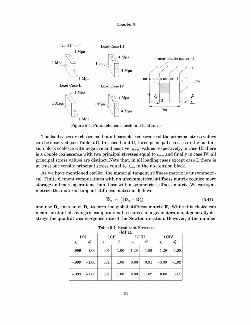
Chapter 5
63
3m
3m
1m23
1
no–tension material
Figure 5.4. Finite element mesh and load cases.
Load Case I
Load Case II
Load Case III
Load Case IV
linear elastic material1 Mpa
1 Mpa
1 Mpa
1 Mpa
1 Mpa
1 Mpa
1 psi
1 Mpa
4 Mpa
4 Mpa
4 Mpa
4 Mpa
The load cases are chosen so that all possible coalescence of the principal stress valuescan be observed (see Table 5.1): In cases I and II, three principal stresses in the no–ten-sion block coalesce with negative and positive (smax) values respectively; in case III thereis a double coalescence with two principal stresses equal to smax and finally in case IV, allprincipal stress values are distinct. Note that, in all loading cases except case I, there isat least one tensile principal stress equal to smax in the no–tension block.
As we have mentioned earlier, the material tangent stiffness matrix is unsymmetri-cal. Finite element computations with an unsymmetrical stiffness matrix require morestorage and more operations than those with a symmetric stiffness matrix. We can sym-metrize the material tangent stiffness matrix as follows
Dm � 12�Dm � DT
m� (5.41)
and use Dm instead of Dm to form the global stiffness matrix Kt. While this choice canmean substantial savings of computational resources in a given iteration, it generally de-stroys the quadratic convergence rate of the Newton iteration. However, if the number
Table 5.1. Resultant Stresses(MPa).
LCI LCII LCIII LCIVsi sh
i si shi sh
isi shisi
–.999
–.999
–.999
–1.00
–1.00
–1.00
.001
.001
.001
1.00
1.00
1.00
–1.29
0.00
0.00
–1.88
0.91
1.62
–1.29
–0.30
0.00
–1.88
–1.09
1.62
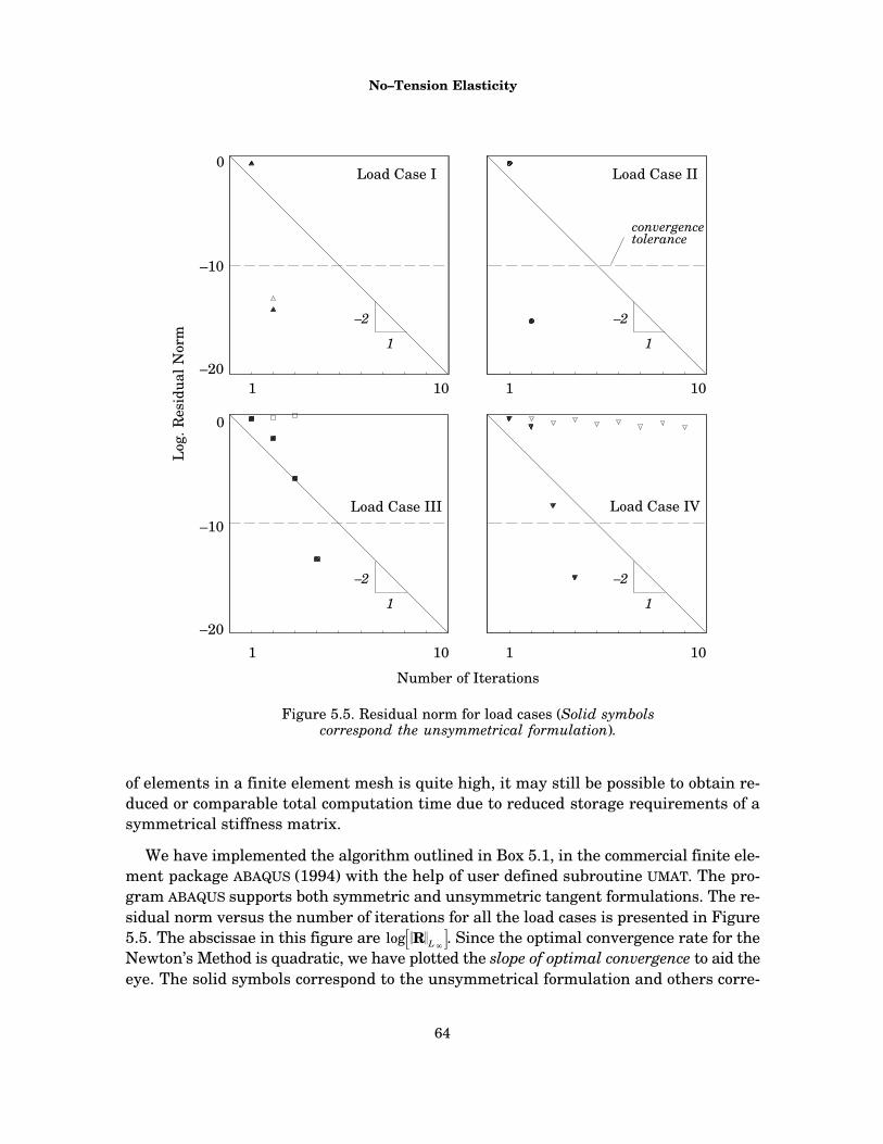
No–Tension Elasticity
64
Load Case I
Load Case III
Load Case II
Load Case IV
1 10 1 10
1 10 1 10
Number of Iterations
0
–20
–10
0
–20
–10
Log
. Res
idua
l Nor
m
–2
1
Figure 5.5. Residual norm for load cases (Solid symbolscorrespond the unsymmetrical formulation).
–2
1
–2
1
–2
1
convergencetolerance
of elements in a finite element mesh is quite high, it may still be possible to obtain re-duced or comparable total computation time due to reduced storage requirements of asymmetrical stiffness matrix.
We have implemented the algorithm outlined in Box 5.1, in the commercial finite ele-ment package ABAQUS (1994) with the help of user defined subroutine UMAT. The pro-gram ABAQUS supports both symmetric and unsymmetric tangent formulations. The re-sidual norm versus the number of iterations for all the load cases is presented in Figure5.5. The abscissae in this figure are log��R�
L��. Since the optimal convergence rate for the
Newton’s Method is quadratic, we have plotted the slope of optimal convergence to aid theeye. The solid symbols correspond to the unsymmetrical formulation and others corre-
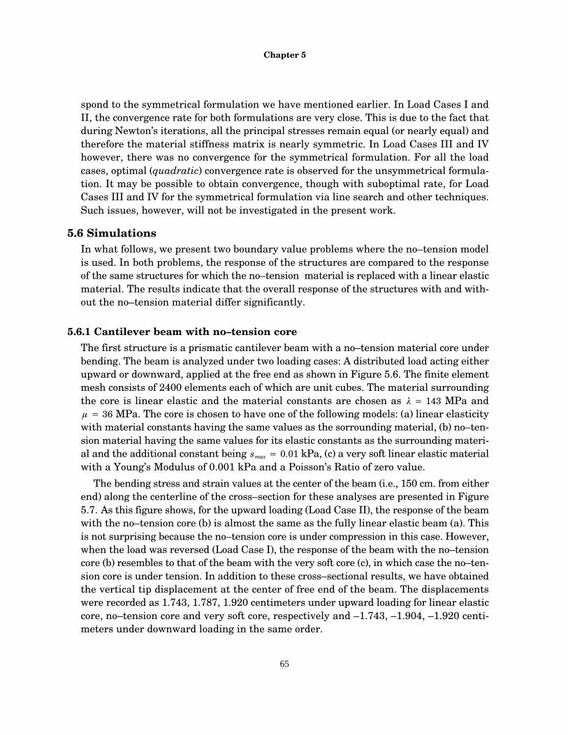
Chapter 5
65
spond to the symmetrical formulation we have mentioned earlier. In Load Cases I andII, the convergence rate for both formulations are very close. This is due to the fact thatduring Newton’s iterations, all the principal stresses remain equal (or nearly equal) andtherefore the material stiffness matrix is nearly symmetric. In Load Cases III and IVhowever, there was no convergence for the symmetrical formulation. For all the loadcases, optimal (quadratic) convergence rate is observed for the unsymmetrical formula-tion. It may be possible to obtain convergence, though with suboptimal rate, for LoadCases III and IV for the symmetrical formulation via line search and other techniques.Such issues, however, will not be investigated in the present work.
5.6 SimulationsIn what follows, we present two boundary value problems where the no–tension modelis used. In both problems, the response of the structures are compared to the responseof the same structures for which the no–tension material is replaced with a linear elasticmaterial. The results indicate that the overall response of the structures with and with-out the no–tension material differ significantly.
5.6.1 Cantilever beam with no–tension coreThe first structure is a prismatic cantilever beam with a no–tension material core underbending. The beam is analyzed under two loading cases: A distributed load acting eitherupward or downward, applied at the free end as shown in Figure 5.6. The finite elementmesh consists of 2400 elements each of which are unit cubes. The material surroundingthe core is linear elastic and the material constants are chosen as � � 143 MPa and� � 36 MPa. The core is chosen to have one of the following models: (a) linear elasticitywith material constants having the same values as the sorrounding material, (b) no–ten-sion material having the same values for its elastic constants as the surrounding materi-al and the additional constant being smax � 0.01 kPa, (c) a very soft linear elastic materialwith a Young’s Modulus of 0.001 kPa and a Poisson’s Ratio of zero value.
The bending stress and strain values at the center of the beam (i.e., 150 cm. from eitherend) along the centerline of the cross–section for these analyses are presented in Figure5.7. As this figure shows, for the upward loading (Load Case II), the response of the beamwith the no–tension core (b) is almost the same as the fully linear elastic beam (a). Thisis not surprising because the no–tension core is under compression in this case. However,when the load was reversed (Load Case I), the response of the beam with the no–tensioncore (b) resembles to that of the beam with the very soft core (c), in which case the no–ten-sion core is under tension. In addition to these cross–sectional results, we have obtainedthe vertical tip displacement at the center of free end of the beam. The displacementswere recorded as 1.743, 1.787, 1.920 centimeters under upward loading for linear elasticcore, no–tension core and very soft core, respectively and –1.743, –1.904, –1.920 centi-meters under downward loading in the same order.
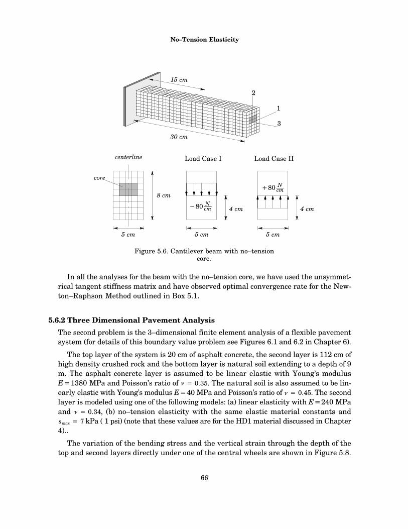
No–Tension Elasticity
66
Figure 5.6. Cantilever beam with no–tensioncore.
8 cm
5 cm
30 cm
centerline
core
15 cm
4 cm�80 Ncm
5 cm
3
1
2
4 cm
�80 Ncm
5 cm
Load Case I Load Case II
In all the analyses for the beam with the no–tension core, we have used the unsymmet-rical tangent stiffness matrix and have observed optimal convergence rate for the New-ton–Raphson Method outlined in Box 5.1.
5.6.2 Three Dimensional Pavement AnalysisThe second problem is the 3–dimensional finite element analysis of a flexible pavementsystem (for details of this boundary value problem see Figures 6.1 and 6.2 in Chapter 6).
The top layer of the system is 20 cm of asphalt concrete, the second layer is 112 cm ofhigh density crushed rock and the bottom layer is natural soil extending to a depth of 9m. The asphalt concrete layer is assumed to be linear elastic with Young’s modulusE�1380 MPa and Poisson’s ratio of � � 0.35. The natural soil is also assumed to be lin-early elastic with Young’s modulus E�40 MPa and Poisson’s ratio of � � 0.45. The secondlayer is modeled using one of the following models: (a) linear elasticity with E�240 MPaand � � 0.34, (b) no–tension elasticity with the same elastic material constants andsmax � 7 kPa ( 1 psi) (note that these values are for the HD1 material discussed in Chapter4)..
The variation of the bending stress and the vertical strain through the depth of thetop and second layers directly under one of the central wheels are shown in Figure 5.8.
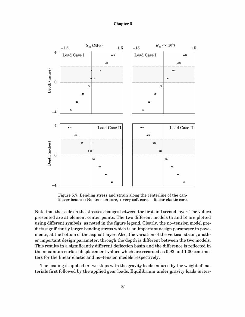
Chapter 5
67
4
–4
0
Dep
th (i
nche
s)
Figure 5.7. Bending stress and strain along the centerline of the can-tilever beam: � No–tension core, + very soft core, � linear elastic core.
4
–4
0
–1.5 1.5D
epth
(inc
hes)
S33 (MPa)–15 15
E33 (� 103)
Load Case II
Load Case ILoad Case I
Load Case II
Note that the scale on the stresses changes between the first and second layer. The valuespresented are at element center points. The two different models (a and b) are plottedusing different symbols, as noted in the figure legend. Clearly, the no–tension model pre-dicts significantly larger bending stress which is an important design parameter in pave-ments, at the bottom of the asphalt layer. Also, the variation of the vertical strain, anoth-er important design parameter, through the depth is different between the two models.This results in a significantly different deflection basin and the difference is reflected inthe maximum surface displacement values which are recorded as 0.93 and 1.00 centime-ters for the linear elastic and no–tension models respectively.
The loading is applied in two steps with the gravity loads induced by the weight of ma-terials first followed by the applied gear loads. Equilibrium under gravity loads is iter-
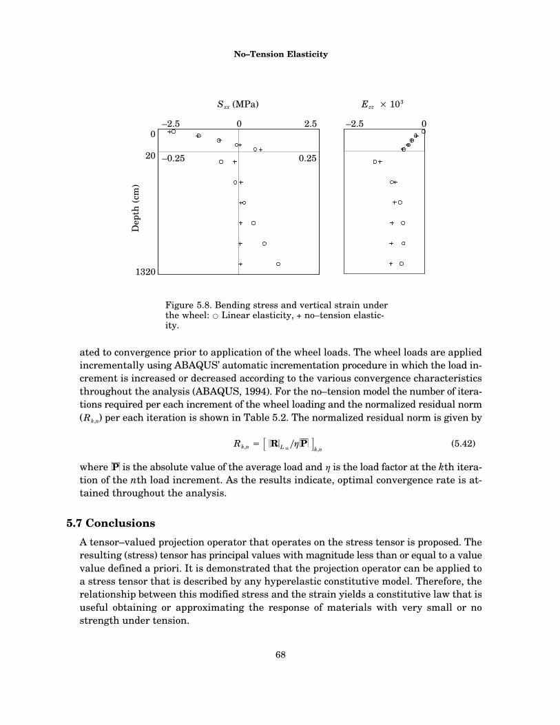
No–Tension Elasticity
68
Figure 5.8. Bending stress and vertical strain underthe wheel: � Linear elasticity, + no–tension elastic-ity.
–2.5 2.5
20
0
1320
Dep
th (
cm)
–0.25 0.25
–2.50 0
Sxx (MPa) Ezz � 103
ated to convergence prior to application of the wheel loads. The wheel loads are appliedincrementally using ABAQUS’ automatic incrementation procedure in which the load in-crement is increased or decreased according to the various convergence characteristicsthroughout the analysis (ABAQUS, 1994). For the no–tension model the number of itera-tions required per each increment of the wheel loading and the normalized residual norm(Rk,n) per each iteration is shown in Table 5.2. The normalized residual norm is given by
Rk,n � � �R�L�
���P� k,n
(5.42)
where �P� is the absolute value of the average load and � is the load factor at the kth itera-tion of the nth load increment. As the results indicate, optimal convergence rate is at-tained throughout the analysis.
5.7 ConclusionsA tensor–valued projection operator that operates on the stress tensor is proposed. Theresulting (stress) tensor has principal values with magnitude less than or equal to a valuevalue defined a priori. It is demonstrated that the projection operator can be applied toa stress tensor that is described by any hyperelastic constitutive model. Therefore, therelationship between this modified stress and the strain yields a constitutive law that isuseful obtaining or approximating the response of materials with very small or nostrength under tension.
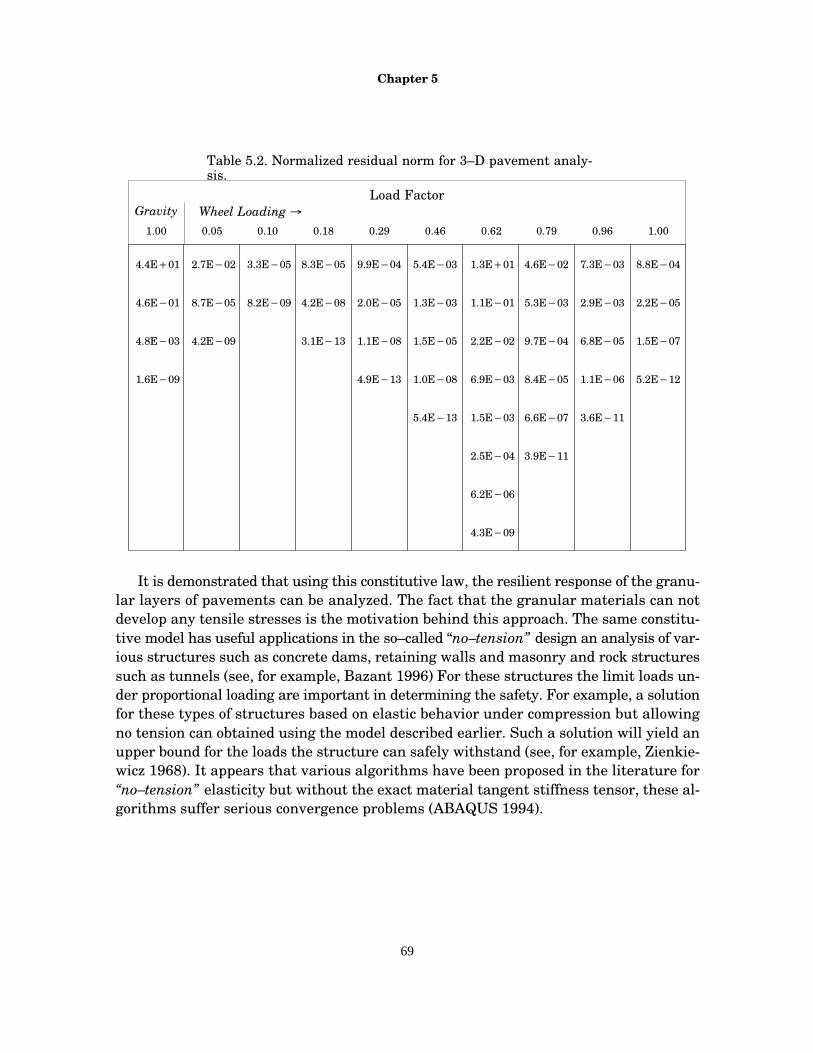
Chapter 5
69
5.3E�03
9.7E�04
6.6E�07
8.4E�05
3.9E�11
4.6E�02
1.1E�01
2.2E�02
1.5E�03
6.9E�03
2.5E�04
6.2E�06
4.3E�09
1.3E�01
Table 5.2. Normalized residual norm for 3–D pavement analy-sis.
4.6E�01
4.4E�01
4.8E�03
8.7E�05
2.7E�02
4.2E�09
8.2E�09 4.2E�08
3.1E�13
2.0E�05
1.1E�08
4.9E�13
1.3E�03
1.5E�05
5.4E�13
1.0E�08
2.9E�03
6.8E�05
3.6E�11
1.1E�06
2.2E�05
1.5E�07
5.2E�12
3.3E�05 8.3E�05 9.9E�04 5.4E�03 7.3E�03 8.8E�04
1.6E�09
1.00 0.05 0.10 0.18 0.29 0.46 0.62 0.79 0.96 1.00
Gravity Wheel Loading �Load Factor
It is demonstrated that using this constitutive law, the resilient response of the granu-lar layers of pavements can be analyzed. The fact that the granular materials can notdevelop any tensile stresses is the motivation behind this approach. The same constitu-tive model has useful applications in the so–called “no–tension” design an analysis of var-ious structures such as concrete dams, retaining walls and masonry and rock structuressuch as tunnels (see, for example, Bazant 1996) For these structures the limit loads un-der proportional loading are important in determining the safety. For example, a solutionfor these types of structures based on elastic behavior under compression but allowingno tension can obtained using the model described earlier. Such a solution will yield anupper bound for the loads the structure can safely withstand (see, for example, Zienkie-wicz 1968). It appears that various algorithms have been proposed in the literature for“no–tension” elasticity but without the exact material tangent stiffness tensor, these al-gorithms suffer serious convergence problems (ABAQUS 1994).

70
Chapter 6
Finite Element Analysis of a Pavement System
In this chapter, the response of three–layered airport pavement under applied loadingis analyzed with the finite element method. The constitutive models presented earlier areused to represent the behavior of the granular layer in this pavement system. Importantdesign parameters such as the bending stress vertical strain at the bottom of the top layerare obtained to compare the predictions of various constitutive models used for the gran-ular layer. The variation of pressure and volumetric strain, octahedral shear stress andstrain through the depth of the granular are presented as well.
6.1 Description of the Pavement System
6.1.1 The Geometry and the LoadingThe pavement system consist of a layer of asphalt concrete on a layer of high densitycrushed rock, on top of natural soil as shown in Fig. 6.1. It is subjected to a loading repre-sentative of a B777–200 type aircraft tridem gear (FAA 1995). The footprint of the load-ing is also shown in Fig. 6.1. The 55 cm � 35 cm rectangular tire prints are assumed tohave a uniform pressure loading of 1.5 MPa. The loading is applied to the center of a 32m � 32 m region.
20 cm
112 cm
Asphalt Concrete
Granular Material
Natural Soil
B777–200 aircraft tridem
Figure 6.1. Flexible pavement system and applied loading
140 cm
145 cm
55 cm
35 cm 145 cm
B777–200 aircraft tridemTire pressure = 1.5 MPa
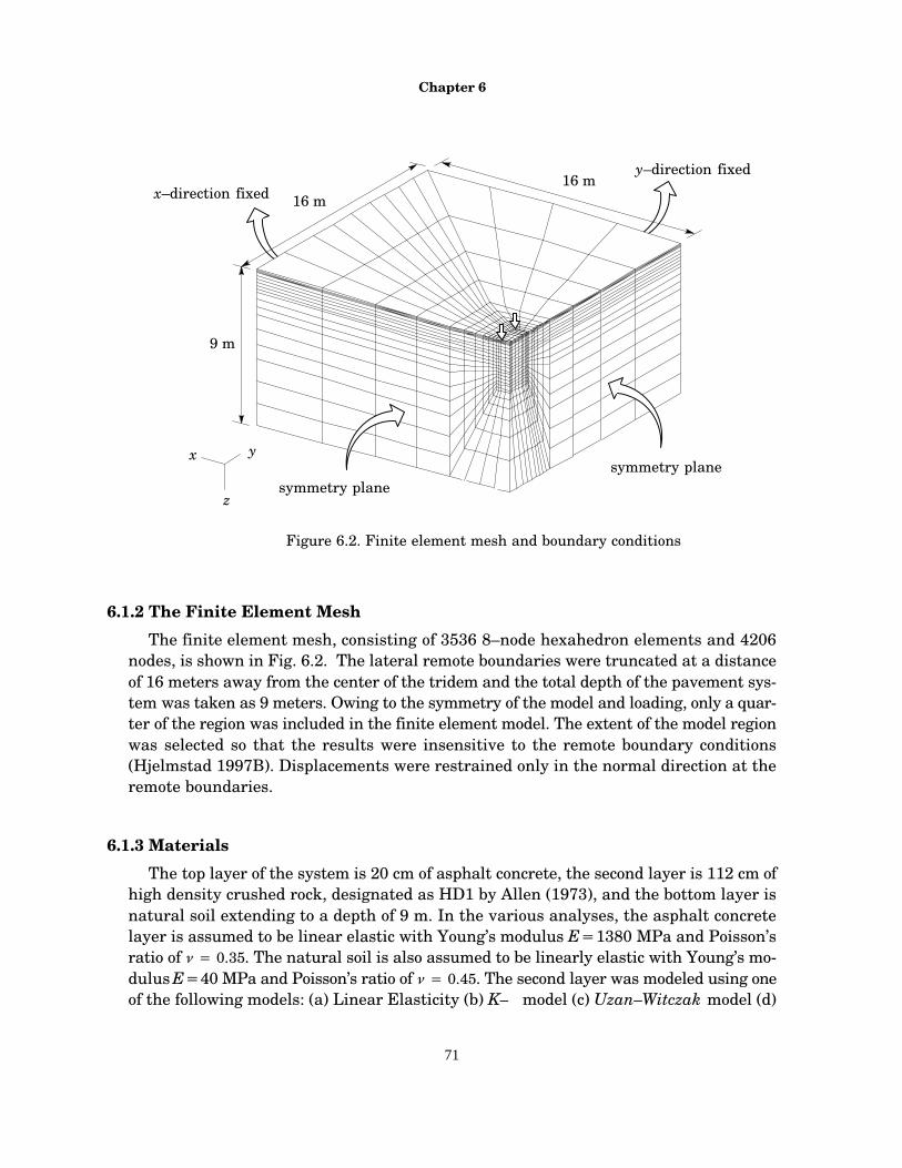
Chapter 6
71
Figure 6.2. Finite element mesh and boundary conditions
x–direction fixed
y–direction fixed
symmetry planesymmetry plane
9 m
16 m16 m
x y
z
6.1.2 The Finite Element Mesh
The finite element mesh, consisting of 3536 8–node hexahedron elements and 4206nodes, is shown in Fig. 6.2. The lateral remote boundaries were truncated at a distanceof 16 meters away from the center of the tridem and the total depth of the pavement sys-tem was taken as 9 meters. Owing to the symmetry of the model and loading, only a quar-ter of the region was included in the finite element model. The extent of the model regionwas selected so that the results were insensitive to the remote boundary conditions(Hjelmstad 1997B). Displacements were restrained only in the normal direction at theremote boundaries.
6.1.3 Materials
The top layer of the system is 20 cm of asphalt concrete, the second layer is 112 cm ofhigh density crushed rock, designated as HD1 by Allen (1973), and the bottom layer isnatural soil extending to a depth of 9 m. In the various analyses, the asphalt concretelayer is assumed to be linear elastic with Young’s modulus E�1380 MPa and Poisson’sratio of � � 0.35. The natural soil is also assumed to be linearly elastic with Young’s mo-dulus E�40 MPa and Poisson’s ratio of � � 0.45. The second layer was modeled using oneof the following models: (a) Linear Elasticity (b) K– � model (c) Uzan–Witczak model (d)

Finite Element Analysis of a Pavement
72
Table 6.2. Material constant values of various constitutive models for the granular layer.
K–� Uzan–Witzcak AD MDNo–Tension
ElasticityLinear
Elasticity
Constitutive Models
E � 240MPa
� � 0.34
K � 170MPa
� � 0.33
n � 0.29
K � 180MPa
� � 0.33
n � 0.22
m � 0.07
K � 170MPa
G � 50MPa
b � 3200GPa
�o � 0 kPa
a � 10000
c � 43GPa
K � 170MPa
G � 50MPa
b � 3200GPa
a � 1000
c � 43GPa
E � 240MPa
� � 0.34
smax � 7 kPa
AD model (described in Chapter 3) (e) MD model (also described in Chapter 3) and finally(f) the no–tension elasticity model described in Chapter 5. The values of the materialconstants for the high density crushed rock material were established by fitting the givenmodel using a weighted nonlinear least-squares curve fitting technique, to the laboratorytest data measured by Allen (1973) (see Chapter 4 for details). The values of the materialconstants of these model are shown in Table 6.2.. The densities of the materials are takento be 0.0024 kgf�cm3 for the asphalt concrete, 0.0022 kgf�cm3 for the crushed rock, and0.0017 kgf�cm3 for the natural soil.
6.2 Results
The variation of the bending stress through the depth of the first (asphalt) layer directlyunder one of the central wheels is shown in Figure 6.3. The variation of the bending stressand the vertical strain through the depth of the second (granular) layer are shown in Fig-ure .6.4 and Figure 6.5 respectively. Note that the scale on the stresses changes betweenthe first and second layer. Finally the variation of pressure, octahedral shear stress, volu-metric strain, and octahedral shear strain are displayed in Figures 6.6, 6.7, 6.8 and 6.9,respectively. The values presented are at element center points. The six different modelsare plotted using different symbols, as noted in the figure legend. The affect of the nonlin-earity is evident in these results.

Chapter 6
73
Figure 6.3. Bending stress in the asphalt layer under the wheel:� K–� model, + Uzan-Witczak model, � MD model, ��AD mod-el, �Linear Elasticity, −�−�−�No–Tension Elasticity.
–2.5 2.5
20
0
Dep
th (
cm)
0
�xx (MPa)
Figure 6.4. Bending stress in the granular layer under thewheel: � K–� model, + Uzan-Witczak model, � MD model,��AD model, �Linear Elasticity, −�−�−�No–Tension Elastic-ity.
–200 200
132
20
Dep
th (
cm)
0
�xx (kPa)
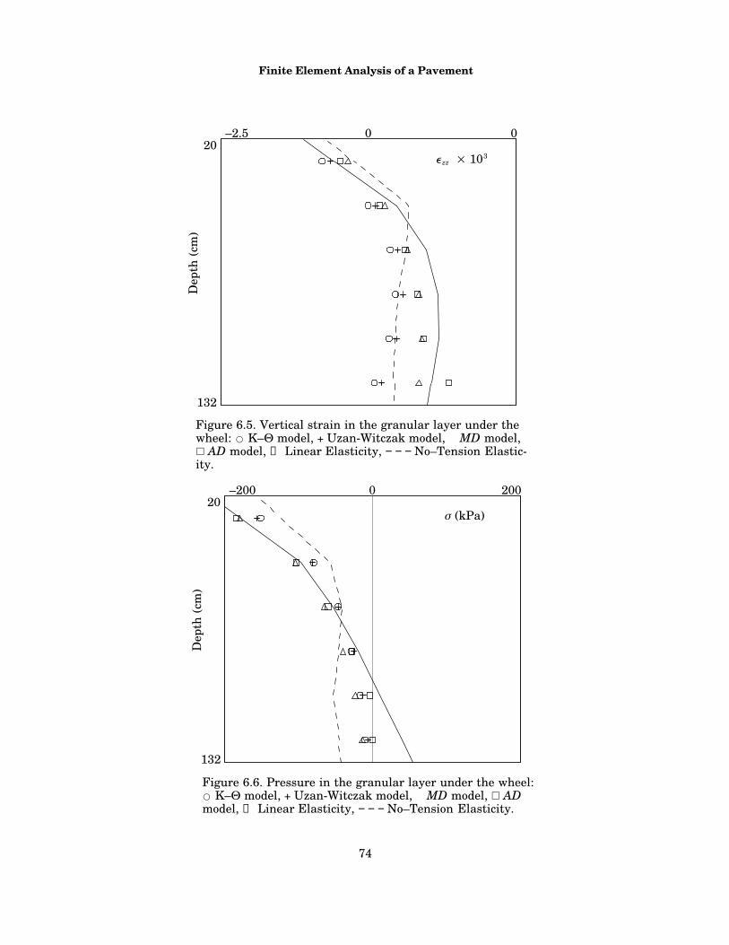
Finite Element Analysis of a Pavement
74
�zz � 103
Figure 6.5. Vertical strain in the granular layer under thewheel: � K–� model, + Uzan-Witczak model, � MD model,��AD model, �Linear Elasticity, −�−�−�No–Tension Elastic-ity.
–2.5 0
132
20
Dep
th (
cm)
0
Figure 6.6. Pressure in the granular layer under the wheel:� K–� model, + Uzan-Witczak model, � MD model, ��ADmodel, �Linear Elasticity, −�−�−�No–Tension Elasticity.
–200 200
132
20
Dep
th (
cm)
0
� (kPa)
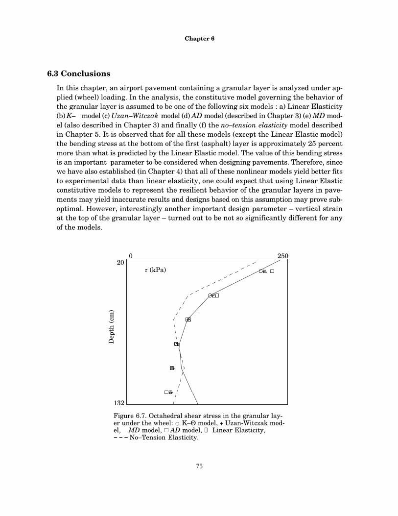
Chapter 6
75
6.3 Conclusions
In this chapter, an airport pavement containing a granular layer is analyzed under ap-plied (wheel) loading. In the analysis, the constitutive model governing the behavior ofthe granular layer is assumed to be one of the following six models : a) Linear Elasticity(b) K– � model (c) Uzan–Witczak model (d) AD model (described in Chapter 3) (e) MD mod-el (also described in Chapter 3) and finally (f) the no–tension elasticity model describedin Chapter 5. It is observed that for all these models (except the Linear Elastic model)the bending stress at the bottom of the first (asphalt) layer is approximately 25 percentmore than what is predicted by the Linear Elastic model. The value of this bending stressis an important parameter to be considered when designing pavements. Therefore, sincewe have also established (in Chapter 4) that all of these nonlinear models yield better fitsto experimental data than linear elasticity, one could expect that using Linear Elasticconstitutive models to represent the resilient behavior of the granular layers in pave-ments may yield inaccurate results and designs based on this assumption may prove sub-optimal. However, interestingly another important design parameter – vertical strainat the top of the granular layer – turned out to be not so significantly different for anyof the models.
Figure 6.7. Octahedral shear stress in the granular lay-er under the wheel: � K–� model, + Uzan-Witczak mod-el, � MD model, ��AD model, �Linear Elasticity,−�−�−�No–Tension Elasticity.
0 250
132
20
Dep
th (
cm)
� (kPa)

Finite Element Analysis of a Pavement
76
It is also observed that the critical response (i.e. the bending stress at the bottom ofthe first layer and the vertical strain at the top of the granular layer) of the pavementpredicted by all the models (except the Linear Elastic model) were nearly identical. How-ever, as this study alone is not a conclusive one regarding the question “which model oneshould choose to represent the behavior of the granular layers ?”, it is important to pointout that for some other pavement configurations (e.g. different thickness for each layer,more layers of different constituents, etc.) it is possible that the nonlinear models mayyield significantly different results. This possibility is evident from the fact that eventhough the response of the top layer was nearly identical for all the nonlinear constitutivemodels, the response of the granular layer (e.g. pressure, volumetric strain, octahedralshear stress and octahedral shear strain) differed significantly among them. Supportingthis argument is the fact that the K– � and Uzan–Witzcak models yielded no hydrostatictension. This is entirely due to the magnitude of the loading, the geometry of the struc-ture and the particular values of the material constants used in the analysis but not dueto any provision in the formulation of these two models that systematically tries to elimi-nate the built up of hydrostatic tension. Therefore, for higher load levels, one could expectthat the K– � and Uzan–Witzcak models will yield tensile hydrostatic pressure within thegranular layer, whereas, models like AD, MD and No–Tension Elasticity will nonethelesstry to reduce the tensile hydrostatic pressure within the granular layer.
� � 103
Figure 6.8. Volumetric strain in the granular layer under thewheel: � K–� model, + Uzan-Witczak model, � MD model,��AD model, �Linear Elasticity, −�−�−�No–Tension Elastic-ity.
–1.0 1.0
132
20
Dep
th (
cm)
0
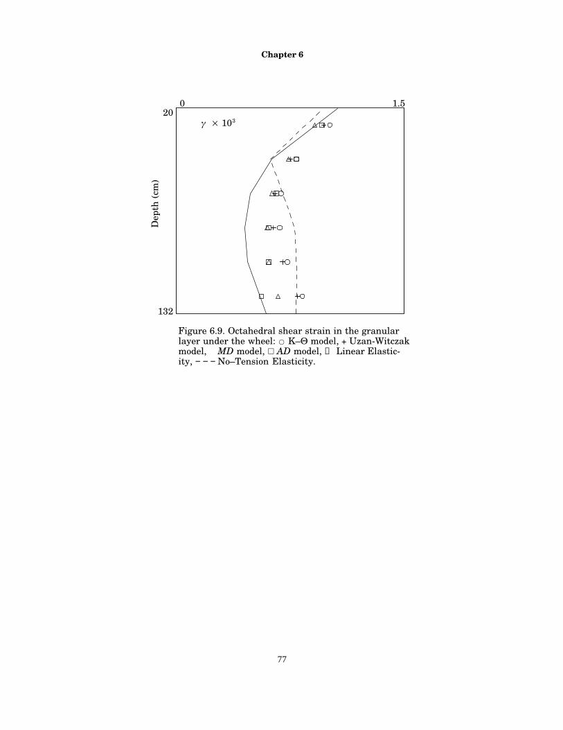
Chapter 6
77
Figure 6.9. Octahedral shear strain in the granularlayer under the wheel: � K–� model, + Uzan-Witczakmodel, � MD model, ��AD model, �Linear Elastic-ity, −�−�−�No–Tension Elasticity.
0 1.5
132
20
Dep
th (
cm)
� � 103

78
Chapter 7
Closure
The conclusions reached in this study have ben presented in the end of every chapterrelevant to the topic of each of them, so they will not be repeated here. A few remarks andsuggestions for future research will be made instead.
The constitutive models investigated or proposed in this study are calibrated using cy-clic triaxial test data alone. The material constants of each of these models can only bedetermined from experiments in which the lateral strain measurements are made. Un-fortunately such experimental data is very scarce. Furthermore, cyclic triaxial testsalone will not be helpful in fully understanding the resilient response; they can not simu-late the stress/strain conditions within the granular layers of pavements where dilationmay occur. For this, experiments are needed in which a well instrumented pavement, ora laboratory size model of a pavement is loaded repeatedly with actual wheel or compac-tion loads.
Built–up of residual stresses within the granular layers of pavements during shake-down is inevitable. This is actually what causes shakedown. The fact that pavements,or their granular layers, respond elastically after a relatively few number of load repeti-tions is an indication of how quickly this process takes place. The presence of residualstresses within the granular layer may well have important implications regarding theoverall response of a pavement. The magnitude and the distribution of the residualstresses can be obtained using plasticity models that take into account the shakedownbehavior. Such a plasticity model can be formulated with yield criteria in terms of princi-pal stresses. The mathematical machinery needed to achieve such a model is very likely,similar to the ones used in formulating the no–tension elasticity model described in Chap-ter 5. Furthermore, the combination of a plasticity model of this sort and the coupled hy-perelastic model presented in Chapter 3 can yield a model which accurately models theresponse of the granular materials during and after the shakedown. The use of plasticitymodels provide a natural setting in eliminating tensile stresses from building up in thefinite element solutions.
The coupled hyperelastic model can also be used in combination with the no–tensionmodel, as the latter one is applicable to any hyperelastic constitutive model. This com-bination will yield accurate representation of the portions of the granular layers that areunder compression and will approximate failure conditions in the remaining portions.

Chapter 7
79
Furthermore, the coupled hyperelastic model itself can be improved easily be introducingdifferent forms of coupling and different terms to the strain energy density function. Asdemonstrated in Chapter 4, the coupled model yielded significantly better fits to the ex-perimental data than any of the other models. This was interpreted as an indication ofthe correctness of the assumption that the volumetric and deviatoric response of granu-lar materials are coupled. As intuition alone is insufficient for developing constitutivemodels., specific experiments are needed to achieve a coupled hyperelastic model that onecan use to determine the specific form and the terms of the strain energy density function.

80
Bibliography
ABAQUS. (1994). Standard User’s Manual, Version 5.4, Volumes 1 & 2. Hibbitt, Karlsson, andSorensen, Inc. Pawtucket, RI.
Allen, J. J. (1973). The effects of non–constant lateral pressures on the resilient response of granu-lar materials. Ph.D. Dissertation, Department of Civil Engineering, University of Illinois, Ur-bana, IL.
Bathe, K. J. (1982). Finite element procedures in engineering analysis. Prentice-Hall, EnglewoodCliffs, N.J. pp. 335–345.
Bazant. (1996). Is No–Tension Design of Concrete Structures Always Safe? Fracture Analysis,J. Structural Eng, 122, pp 2–10.
Boussinesq, J. (1885). Application des potentiels a l’etude de l’eequilibre et du mouvement des sol-ids elastiques. Gauthier–Villars, Paris.
Boyce, J. R. (1980). A nonlinear model for the elastic behavior of granular materials under re-peated loading. Proceedings of the International Symposium on Soils Under Cyclic and TransientLoading, Swansea.
Brown, S. F. and Pappin, J. W. (1981). Analysis of pavements with granular bases. Transporta-tion Research Record 810. pp. 17–23.
Burmister, D. M. (1945). The general theory of stresses and displacements in layered soil systems,I, II, and III. Journal of Applied Physics, 16. pp. 84–94 (I), 126–127 (II), 296–302 (III).
Carlson D. E. and Hoger, A. (1986). The derivative of a tensor–valued function of a tensor. Quart.Appl. Math., XLIV, No. 3, 409–423.
Chen, W. F. and A. F. Saleeb, (1994) Constitutive Equations for Engineering Materials, Volumes1 & 2, Revised Edition, Elsevier.
Crisfield, M. A. (1991). Non–linear finite element analysis of solids and structures. Volume 1: Es-sentials. John Wiley & Sons. pp. 132–134, 154–155.
De Jong, D. L., Peatz, M. G. F. and Korswagen, A. R. (1972). Computer program BISAR: Layeredsystems under normal and tangential loads, Koninklijke Shell–Laboratorium, Amsterdam, Ex-ternal Report AMSR.0006.73.
Del Piero, G. (1989). Constitutive equation and compatibility of the external loads for linear elas-tic masonry–like materials. Meccanica, 24, 150–162.

Appendix I
81
Desai, C. S. and H. J. Siriwardane, (1984) Constitutive Laws for Engineering Materials, WithEmphasis on Geologic Materials, Prentice-Hall, Inc., Englewood Cliffs, New Jersey.
Domaschuk, L., Valiappan, P., (1975). Nonlinear settlement analysis by finite elements. Journalof the Geotechnical Engineering , ASCE, 101(GT7), 601–614.
Duncan, J. M., Monismith, C. L. and Wilson, E. L. (1968). Finite element analyses of pavements.Highway Research Record 228. pp. 18–33.
FAA. (1995). Advisory Circular (AC) No: 150/5320–16. Airport pavement design for the Boeing777 airplane. Federal Aviation Administration, U.S. Department of Transportation, WashingtonD.C.
Fletcher, R. (1987). Practical methods of optimization, Second Edition, John Wiley & Sons. NewYork.
Guterl, F. (1997), Riddles in the Sand, Discover Magazine, November, pp. 104–114.
Halmos, P. R. (1958). Finite–dimensional vector spaces. 2nd Ed., D. Van Nostrand, Princeton NJ.
Harichandran, R. S., Yeh, M. S. and Baladi, G. Y. (1971). MICH–PAVE: A nonlinear finite ele-ment program for analysis of pavements. Transportation Research Record 345. pp. 15–31.
Harr, M. E. (1977), Mechanics of Particulate Media — A Probabilistic Approach, McGraw HillBook Company, Inc., New York.
Heath, M. T. (1997). Scientific computing. An introductory survey. McGraw-Hill. New York.
Hicks, R. G. and Monismith, C. L. (1971). Factors influencing the resilient properties of granularmaterials. Transportation Research Record 345. pp. 15–31.
Hjelmstad, K. D. (1997A). Fundamentals of structural mechanics. Prentice Hall, Upper SaddleRiver, New Jersey.
Hjelmstad, K. D., J. Kim, and Q. H. Zuo. (1997B). Finite element procedures for three dimensionalpavement analysis. Aircraft/Pavement Technology: In the Midst of Change (F. V. Hermann, ed.).Proceedings of the ASCE 1997 Airfield Pavement Conference. August 17–20, 1997. Seattle,Washington. pp. 125–137.
Huang, Y. H. (1993). Pavement analysis and design. Prentice Hall, Englewood Cliffs, NJ.
Hughes, T. J. R. (1987). The Finite Element Method. Prentice-Hall, Englewood Cliffs, N.J..
Izumi, H. K., Kamemura K. and Sato S., (1976). Finite element analysis of stresses and move-ments in excavations. Numerical Methods in Geomechanics, ASCE, 701–712.
Jeffrey, A. (1995). Handbook of Mathematical Formulas and Integrals. Academic Press, Inc., SanDiego, CA. pp. 394–395.
Appendix I
82
Kato, T. (1976). Perturbation Theory for Linear Operators. 2nd Ed., Springer, Berlin–Heidel-berg–New York.
Ko, H. Y., Scott, R. F., (1967). Deformation of sand in shear. Journal of the Soil Mech. Founda-tions Div., ASCE, 93(SM5), 283–310.
Kooperman, S., Tiller, G. and Tseng, M. (1986). ELSYM5, Interactive microcomputer version,User’s Manual. Report No. FHWA–TS–87–206, Federal Highway Administration, Washington,D.C.
Lade, P. V., Nelson R. B., (1987). Modelling the elastic behavior of granular materials, Int. J.Num. Anal. Methods Geomech., 11, 521–542.
Lade, P. V., (1988). Effect of voids and volume changes on the behavior of frictional materials.Int. J. Num. Analytical Methods Geomech., 12, pp 331–370.
May, R. W. and Witczak, M. W. (1981). Effective granular modulus to model pavement responses.Transportation Research Record 810. pp. 1–9.
Raad, L. and Figueroa, J. L. (1980). Load response of transportation support systems. Transporta-tion Engineering Journal, ASCE, 16 (TE1). pp. 111–128.
Schreyer, H. L. and Zuo, Q. H. (1995). Anisotropic yield surfaces based on elastic projection opera-tors. J. Applied Mech., v. 62, pp. 780–785.
Simo, J. C. and Taylor, R. L. (1991). Quasi–incompressible finite elasticity in principal stretches.Continuum basis and numerical algorithms. Comp. Meth. Appl. Mech Eng., v. 85. 273–310.
Sokolnikoff, I. S., (1983) Mathematical Theory of Elasticity, Krieger Publishing Company, Inc.,Malabar, Florida, Reprint Edition, pp. 339–343.
Truesdell, C. and Noll, W. (1965). The Non–linear Field Theories of Mechanics, Encyclopedia ofPhysics, III / 3, Springer, Berlin.
Tutumluer, E. (1995). Predicting behavior of flexible pavements with granular bases. Ph.D. The-sis. Georgia Institute of Technology.
Uzan, J. (1985). Characterization of granular materials. Transportation Research Record 1022.pp. 52–59.
Warren, H. and Dieckman, W. L. (1963). Numerical computation of stresses and strains in a mul-tiple–layer asphalt pavement system. International Report, Chevron Research Corporation,Richmond, CA.
Westergaard, H. M., (1947) New Formulas for Stresses in Concrete Runways of Airports, Proceed-ings, 113, ASCE.
Witczak, M. W. and Uzan, J. (1988). The universal airport pavement design system. Report I ofV: Granular material characterization. University of Maryland, Department of Civil Engineer-ing, MD.

Appendix I
83
Zienkiewicz, O. C., Valiappan, S. and King, I. P. (1968). Stress analysis of rock as a “no tension”material. Géotechnique. 18: 50. 56–66.

84
Appendix
I. A Brief Overview of ABAQUS UMATUser subroutines in ABAQUS provide an extremely powerful and flexible tool for analy-sis. The user–defined subroutine UMAT enables one to implement material behaviorthat are not found in ABAQUS material library. The use of UMAT requires great care.It must perform the intended function without interfering with other functions and with-out overwriting unintended arrays of ABAQUS.
The interface card for the user–subroutine UMAT is as follows.
subroutine umat (stress, statev, ddsdde, & sse, spd, scd, rpl, ddsddt, drplde,
& drpldt, stran, dstran, time, & dtime, temp, dtemp, predef, dpred,
& cmname, ndi, nshr, ntens, nstatv, & props, nprops, coords, drot,
& pnewdt, celent,dfgrd0, dfgrd1, noel, & npt, layer, kspt, kstep, kinc )
include ’ABA_PARAM.INC’
character*8 cmname dimension stress(ntens), statev(nstatv),
& ddsdde(ntens, ntens), & ddsddt(ntens), drplde(ntens),
& stran(ntens), dstran(ntens), time(2), & predef(*), dpred(*),
& props(nprops), coords(3), drot(3, 3), & dfgrd0(3, 3), dfgrd1(3, 3)
The variables and arrays to be defined by this subroutine are <ddsdde> and <stress>.The variables and arrays that may be defined optionally are <statev>, <sse>, <spd> and<scd>. All the remaining argument variables are passed in for data and overwriting themwill cause an error.
The two–dimensional array <ddsdde> is the material stiffness matrix. In other words,it is the Jacobian matrix of the constitutive model. The size of this array (per gauss point)is defined by the variable <ntens>. This integer–valued variable is generally different foreach type of element. For 3–dimensional elements its value is usually 6, for axisymmetricelements it is 5. It also defines the size of the <stress> in which the stresses are stored.The subroutine must define every element of <ddsdde> regardless of symmetry. If it is

Appendix I
85
unsymmetrical, user can request in the input file, unsymmetrical storage and solver.This is achieved by specifying in the input file at the header,
*HEADING, UNSYMM, ... etc.
and in the material definition,
*USER MATERIAL, UNSYMMETRIC, ... etc.
However, since this will invoke the unsymmetric solver in ABAQUS and force ABAQUSto use unsymmetric storage the computations will take more time. Note that, ABAQUSassumes symmetric storage and solver by default.
The one–dimensional arrays <stran> and <dstran> contain the strain and incremen-tal strain array respectively. Since the stresses must be computed using the total strainvalues, for elastic constitutive models, we need to add these two arrays to get the currentiterative value of the strain.
The array <props> passes the information specified by user in input file. The contentsof this array are usually the material parameters. The size of <props> is defined by theinteger–valued variable <nprops> which is also specified in the input file. For example,
*USER MATERIAL, CONSTANTS = 710000, .35, .22, .7, 50000., 1., 0.
where 7 defines the value of <nprops> and the seven values in the second card above arethe values of the material constants which will be stored in the array <props>. For exam-ple in our implementation of the K– � and Uzan–Witzcak models these values are k, � , m,n, E, damping_factor, secant_switch (for details see Appendix II).
The use of one dimensional array <statev> is optional. One can use this array to storesolution dependent values for each gauss point. This array is overwritten after every loadincrement but not at every equilibrium iteration. The size of <statev> is defined by theinteger–valued variable <nstatev> which can be specified in input file via card,
*USER MATERIAL, UNSYMMETRIC, ... etc.
... etc.*DEPVAR
20
The value 20 above is the size of <statev> array. Thus, ABAQUS will reserve space forstoring 20 entries for every gauss point. In our implementation of the K– � and Uzan–Witzcak models, we have used this array to store the resilient moduli of every gauss pointso that we could use visualization tools (such as ABAQUS–POST or PATRAN ) to plotthe resilient modulus distribution for any desired load increment. The values stored in<statev> can be output via card in input file

Appendix I
86
*EL FILE
SDV
If needed, one can create debug output for user–defined subroutines. This output canbe written to FORTRAN unit 7 to appear on the .msg file, or to FORTRAN unit 6 to ap-pear on the .dat file. FORTRAN units 15 through 18 may also be used to read or writeother user–specified information. ABAQUS manual warns that the use of other FOR-TRAN units may interfere with ABAQUS file operations. In our implementation we havechosen unit 7 ( .msg file) to write the debug output.
The source code for the K– � and Uzan–Witzcak models discussed in Chapter 2 can befound in Appendix II as an example. The UMAT subroutine for all the other models pres-ented in this manuscript are omitted for brevity.
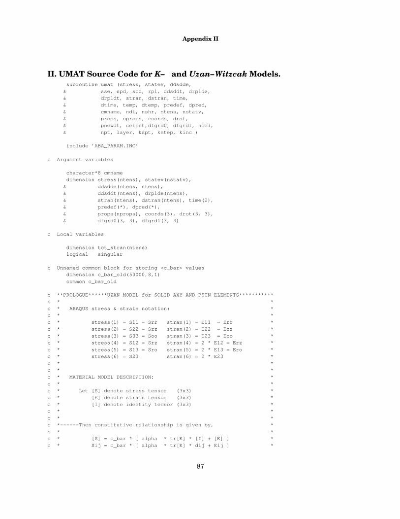
Appendix II
87
II. UMAT Source Code for K– � and Uzan–Witzcak Models. subroutine umat (stress, statev, ddsdde,
& sse, spd, scd, rpl, ddsddt, drplde, & drpldt, stran, dstran, time,
& dtime, temp, dtemp, predef, dpred, & cmname, ndi, nshr, ntens, nstatv,
& props, nprops, coords, drot, & pnewdt, celent,dfgrd0, dfgrd1, noel,
& npt, layer, kspt, kstep, kinc )
include ’ABA_PARAM.INC’
c Argument variables
character*8 cmname dimension stress(ntens), statev(nstatv),
& ddsdde(ntens, ntens), & ddsddt(ntens), drplde(ntens),
& stran(ntens), dstran(ntens), time(2), & predef(*), dpred(*),
& props(nprops), coords(3), drot(3, 3), & dfgrd0(3, 3), dfgrd1(3, 3)
c Local variables
dimension tot_stran(ntens) logical singular
c Unnamed common block for storing <c_bar> values dimension c_bar_old(50000,8,1)
common c_bar_old
c **PROLOGUE******UZAN MODEL for SOLID AXY AND PSTN ELEMENTS***********c * *
c * ABAQUS stress & strain notation: *c * *
c * stress(1) = S11 = Srr stran(1) = E11 = Err *c * stress(2) = S22 = Szz stran(2) = E22 = Ezz *
c * stress(3) = S33 = Soo stran(3) = E23 = Eoo *c * stress(4) = S12 = Srz stran(4) = 2 * E12 = Erz *
c * stress(5) = S13 = Sro stran(5) = 2 * E13 = Ero *c * stress(6) = S23 stran(6) = 2 * E23 *
c * *c * *
c * MATERIAL MODEL DESCRIPTION: *c * *
c * Let [S] denote stress tensor (3x3) *c * [E] denote strain tensor (3x3) *
c * [I] denote identity tensor (3x3) *c * *
c * *c *––––––Then constitutive relationship is given by, *
c * *c * [S] = c_bar * [ alpha * tr[E] * [I] + [E] ] *
c * Sij = c_bar * [ alpha * tr[E] * dij + Eij ] *
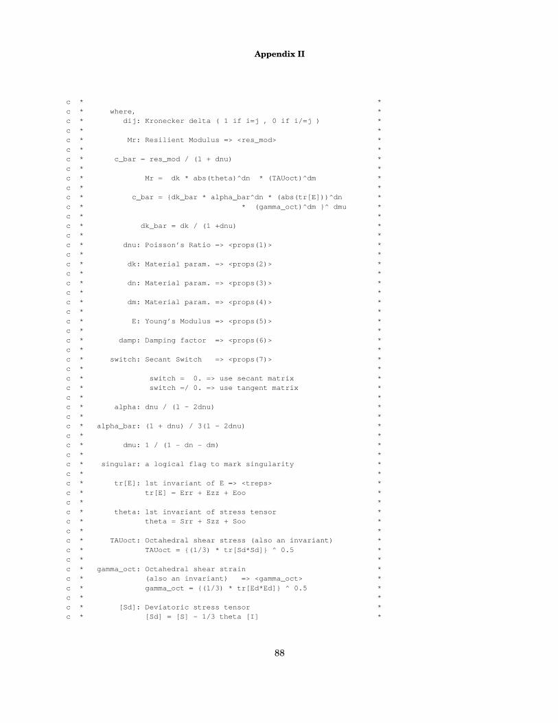
Appendix II
88
c * *
c * where, *c * dij: Kronecker delta ( 1 if i=j , 0 if i/=j ) *
c * *c * Mr: Resilient Modulus => <res_mod> *
c * *c * c_bar = res_mod / (1 + dnu) *
c * *c * Mr = dk * abs(theta)^dn * (TAUoct)^dm *
c * *c * c_bar = {dk_bar * alpha_bar^dn * (abs(tr[E]))^dn *
c * * (gamma_oct)^dm }^ dmu *c * *
c * dk_bar = dk / (1 +dnu) *c * *
c * dnu: Poisson’s Ratio => <props(1)> *c * *
c * dk: Material param. => <props(2)> *c * *
c * dn: Material param. => <props(3)> *c * *
c * dm: Material param. => <props(4)> *c * *
c * E: Young’s Modulus => <props(5)> *c * *
c * damp: Damping factor => <props(6)> *c * *
c * switch: Secant Switch => <props(7)> *c * *
c * switch = 0. => use secant matrix *c * switch =/ 0. => use tangent matrix *
c * *c * alpha: dnu / (1 – 2dnu) *
c * *c * alpha_bar: (1 + dnu) / 3(1 – 2dnu) *
c * *c * dmu: 1 / (1 – dn – dm) *
c * *c * singular: a logical flag to mark singularity *
c * *c * tr[E]: 1st invariant of E => <treps> *
c * tr[E] = Err + Ezz + Eoo *c * *
c * theta: 1st invariant of stress tensor *c * theta = Srr + Szz + Soo *
c * *c * TAUoct: Octahedral shear stress (also an invariant) *
c * TAUoct = {(1/3) * tr[Sd*Sd]} ^ 0.5 *c * *
c * gamma_oct: Octahedral shear strain *c * (also an invariant) => <gamma_oct> *
c * gamma_oct = {(1/3) * tr[Ed*Ed]} ^ 0.5 *c * *
c * [Sd]: Deviatoric stress tensor *c * [Sd] = [S] – 1/3 theta [I] *

Appendix II
89
c * *
c * [Ed]: Deviatoric strain tensor *c * [Ed] = [E] – 1/3 tr[E] [I] *
c * *c * *
c *––––––Material tangent stiffness [C] *c * *
c * C = d([S]) / d([E]) *c * Cijkl = d([Sij]) / d([Ekl]) *
c * *c * thus, with summation implied over repeated *
c * indices, i;j;k;l = {1,2,3} *c * *
c * Sij = Cijkl Ekl *c * *
c * Cijkl = c_bar { dik * djl *c * + A dij * dkl *
c * + B Eij * dkl *c * + C dij * Ekl *
c * + D Eij * Ekl } *c * *
c * where, *c * A = alpha * ( dmu * x + 1) *
c * B = D * alpha * (tr[E]) *c * C = dmu * dm / (3*gamma_oct^2) *
c * D = dmu * x / (tr[E]) *c * x = dn – dm * ( tr[E]/ 3gamma_oct) ^2 *
c * *c * Or in matrix notation, *
c * *c * vec(S) = mat(C) * vec(E) *
c * *c * where, *
c * vec(S): Stress vector => <stress> *c * vec(E): Strain vector => <tot_stran> *
c * mat(C): Material tnagent dtiffness matrix => <ddsdde> *c * *
c * *c * 1 1 1 0 0 0 *
c * 1 1 1 0 0 0 *c * 1 1 1 0 0 0 *
c * mat(dijdkl) = *c * 0 0 0 0 0 0 *
c * 0 0 0 0 0 0 *c * 0 0 0 0 0 0 *
c * *c * *
c * 1 0 0 0 0 0 *c * 0 1 0 0 0 0 *
c * 0 0 1 0 0 0 *c * mat(dikdjl) = *
c * 0 0 0 .5 0 0 *c * 0 0 0 0 .5 0 *
c * 0 0 0 0 0 .5 *c * *
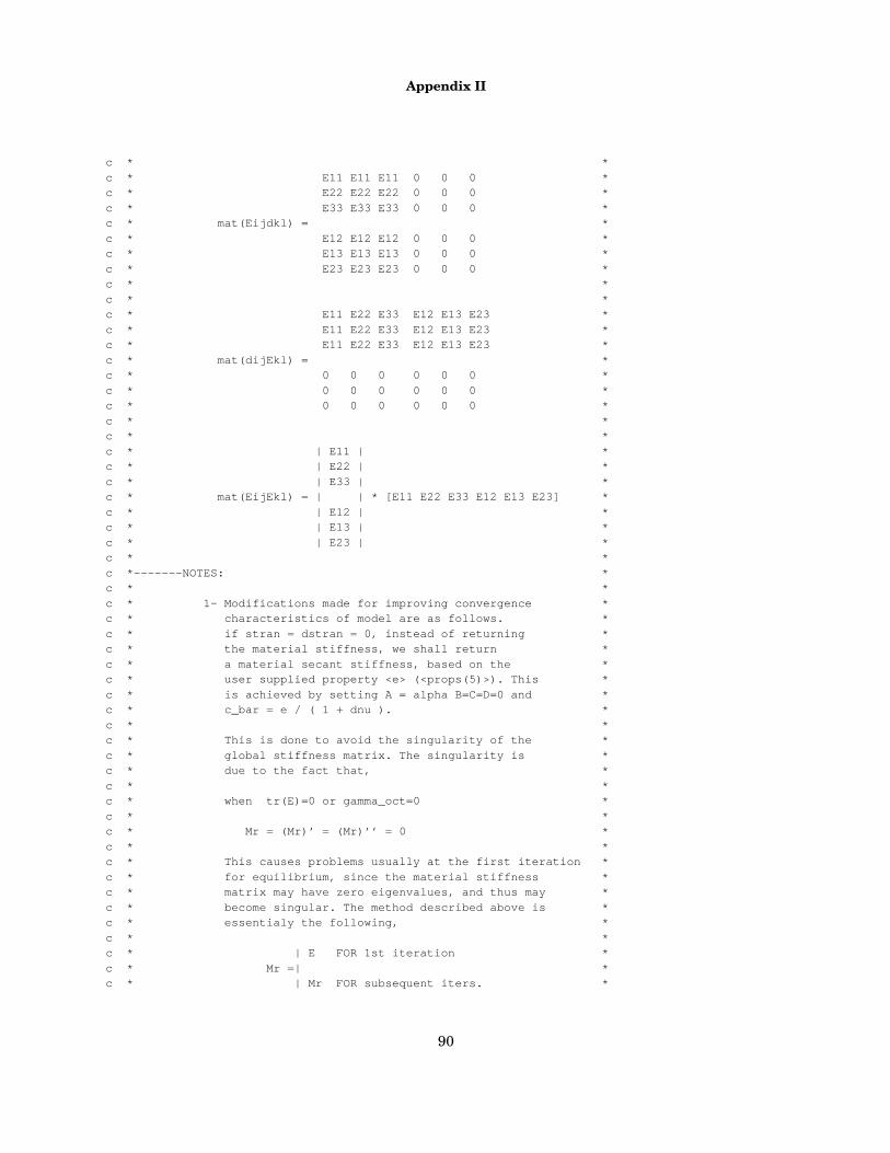
Appendix II
90
c * *
c * E11 E11 E11 0 0 0 *c * E22 E22 E22 0 0 0 *
c * E33 E33 E33 0 0 0 *c * mat(Eijdkl) = *
c * E12 E12 E12 0 0 0 *c * E13 E13 E13 0 0 0 *
c * E23 E23 E23 0 0 0 *c * *
c * *c * E11 E22 E33 E12 E13 E23 *
c * E11 E22 E33 E12 E13 E23 *c * E11 E22 E33 E12 E13 E23 *
c * mat(dijEkl) = *c * 0 0 0 0 0 0 *
c * 0 0 0 0 0 0 *c * 0 0 0 0 0 0 *
c * *c * *
c * | E11 | *c * | E22 | *
c * | E33 | *c * mat(EijEkl) = | | * [E11 E22 E33 E12 E13 E23] *
c * | E12 | *c * | E13 | *
c * | E23 | *c * *
c *–––––––NOTES: *c * *
c * 1– Modifications made for improving convergence *c * characteristics of model are as follows. *
c * if stran = dstran = 0, instead of returning *c * the material stiffness, we shall return *
c * a material secant stiffness, based on the *c * user supplied property <e> (<props(5)>). This *
c * is achieved by setting A = alpha B=C=D=0 and *c * c_bar = e / ( 1 + dnu ). *
c * *c * This is done to avoid the singularity of the *
c * global stiffness matrix. The singularity is *c * due to the fact that, *
c * *c * when tr(E)=0 or gamma_oct=0 *
c * *c * Mr = (Mr)’ = (Mr)’’ = 0 *
c * *c * This causes problems usually at the first iteration *
c * for equilibrium, since the material stiffness *c * matrix may have zero eigenvalues, and thus may *
c * become singular. The method described above is *c * essentialy the following, *
c * *c * | E FOR 1st iteration *
c * Mr =| *c * | Mr FOR subsequent iters. *
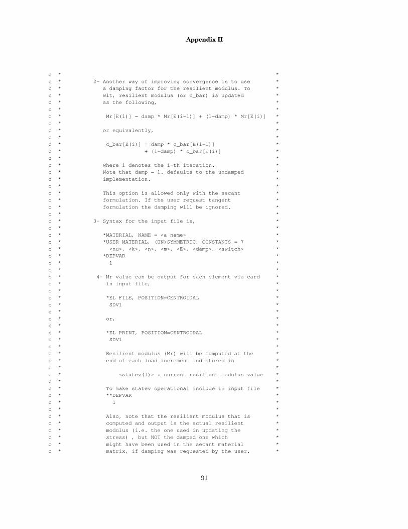
Appendix II
91
c * *
c * 2– Another way of improving convergence is to use *c * a damping factor for the resilient modulus. To *
c * wit, resilient modulus (or c_bar) is updated *c * as the following, *
c * *c * Mr[E(i)] = damp * Mr[E(i–1)] + (1–damp) * Mr[E(i)] *
c * *c * or equivalently, *
c * *c * c_bar[E(i)] = damp * c_bar[E(i–1)] *
c * + (1–damp) * c_bar[E(i)] *c * *
c * where i denotes the i–th iteration. *c * Note that damp = 1. defaults to the undamped *
c * implementation. *c * *
c * This option is allowed only with the secant *c * formulation. If the user request tangent *
c * formulation the damping will be ignored. *c * *
c * 3– Syntax for the input file is, *c * *
c * *MATERIAL, NAME = <a name> *c * *USER MATERIAL, (UN)SYMMETRIC, CONSTANTS = 7 *
c * <nu>, <k>, <n>, <m>, <E>, <damp>, <switch> *c * *DEPVAR *
c * 1 *c * *
c * 4– Mr value can be output for each element via card *c * in input file, *
c * *c * *EL FILE, POSITION=CENTROIDAL *
c * SDV1 *c * *
c * or, *c * *
c * *EL PRINT, POSITION=CENTROIDAL *c * SDV1 *
c * *c * Resilient modulus (Mr) will be computed at the *
c * end of each load increment and stored in *c * *
c * <statev(1)> : current resilient modulus value *c * *
c * To make statev operational include in input file *c * **DEPVAR *
c * 1 *c * *
c * Also, note that the resilient modulus that is *c * computed and output is the actual resilient *
c * modulus (i.e. the one used in updating the *c * stress) , but NOT the damped one which *
c * might have been used in the secant material *c * matrix, if damping was requested by the user. *

Appendix II
92
c * *
c ****************************************************END*PROLOGUE*****
c *********************************************************************c * copyright : E. Taciroglu, K. D. Hjelmstad –1997 *
c * references : 1– ABAQUS USER’S MANUAL, Ver. 5.4, Vol. II, *c *********************************************************************
c Initialize Material Properties
dnu = props(1) dk = props(2)
dn = props(3) dm = props(4)
e = props(5) damp = props(6)
switch = props(7)
alpha = dnu / (1. – 2.*dnu) alpha_bar = (1. + dnu)/ ( 3. * (1. – 2. * dnu))
dmu = 1. / (1. – dn – dm) dk_bar = dk / (1. + dnu)
c Get total strain vector and strain invariants tr(E), gamma_oct
tot_stran(1:ndi) = stran(1:ndi) + dstran(1:ndi) tot_stran(ndi+1:) = (stran(ndi+1:) + dstran(ndi+1:)) / 2.
treps = tot_stran(1) + tot_stran(2) + tot_stran(3)
gamma_oct = 0.
do i=1,ndi
gamma_oct = gamma_oct + tot_stran(i)**2. end do
do i=ndi+1,ntens gamma_oct = gamma_oct + 2.*tot_stran(i)**2.
end do gamma_oct = gamma_oct – treps**2. / 3.
gamma_oct = sqrt(gamma_oct/3.)
c Update Resilient modulus
c_bar = dk_bar * alpha_bar**dn * abs(treps)**dn * gamma_oct**dm c_bar = c_bar ** dmu
res_mod = c_bar * (1. + dnu)
c Select appropriate modulus value <c_bar> for <ddsdde> and <stress>
singular = .true.
do i=1,ntens if(tot_stran(i).ne.0.) singular = .false.
end do
if(singular) then
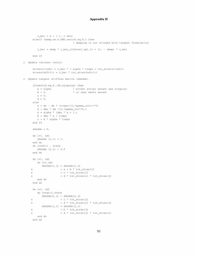
Appendix II
93
c_bar = e / ( 1. + dnu)
elseif (damp.ne.0.AND.switch.eq.0.) then ! damping is not allowed with tangent formulation
c_bar = damp * c_bar_old(noel,npt,1) + (1. – damp) * c_bar
end if
c Update <stress> vector
stress(1:ndi) = c_bar * ( alpha * treps + tot_stran(1:ndi)) stress(ndi+1:) = c_bar * tot_stran(ndi+1:)
c Update tangent stiffnes matrix <ddsdde>
if(switch.eq.0..OR.singular) then
a = alpha ! either actual secant was singular b = 0. ! or user wants secant
c = 0. d = 0.
else x = dn – dm * (treps/(3.*gamma_oct))**2.
d = dmu * dm /(3.*gamma_oct**2.) a = alpha * (dmu * x + 1.)
b = dmu * x / treps c = d * alpha * treps
end if
ddsdde = 0.
do i=1, ndi ddsdde (i,i) = 1.
end do do i=ndi+1 , ntens
ddsdde (i,i) = 0.5 end do
do i=1, ndi
do j=1,ndi ddsdde(i,j) = ddsdde(i,j)
& + a + b * tot_stran(i) & + c * tot_stran(j)
& + d * tot_stran(i) * tot_stran(j) end do
end do
do i=1, ndi
do j=ndi+1,ntens ddsdde(i,j) = ddsdde(i,j)
& + c * tot_stran(j) & + d * tot_stran(i) * tot_stran(j)
ddsdde(j,i) = ddsdde(j,i) & + b * tot_stran(j)
& + d * tot_stran(j) * tot_stran(i) end do
end do

Appendix II
94
do i=ndi+1, ntens
do j=ndi+1, ntens ddsdde(i,j) = ddsdde(i,j) + d * tot_stran(i) * tot_stran(j)
end do end do
ddsdde = c_bar * ddsdde
c Debugging statements (will be written to .msg file)
if(noel.eq.1121.AND.npt.eq.1) then
write(7,*) ’ **UMAT*************************DEBUG***’ write(7,*) ’ >>>> reporting gauss pt.’,npt
write(7,*) write(7,*) ’ time(1) = ’, time(1)
write(7,*) ’ time(2) = ’, time(2) write(7,*) ’ kstep = ’, kstep
write(7,*) ’ kinc = ’, kinc write(7,*) ’ nu = ’, dnu
write(7,*) ’ k = ’, dk write(7,*) ’ k_bar = ’, dk_bar
write(7,*) ’ n = ’, dn write(7,*) ’ m = ’, dm
write(7,*) ’ e = ’, e write(7,*) ’ damp = ’, damp
write(7,*) ’ switch = ’, switch write(7,*) ’ alpha = ’, alpha
write(7,*) ’ alpha_bar = ’, alpha_bar write(7,*) ’ dmu = ’, dmu
write(7,*) ’ treps = ’, treps write(7,*) ’ gamma_oct = ’, gamma_oct
write(7,*) ’ c_bar = ’, c_bar write(7,*) ’ c_bar_old = ’, c_bar_old(noel,npt,1)
write(7,*) ’ res_mod = ’, res_mod write(7,*) ’ statev(1) = ’, statev(1)
if(switch.eq.0.) then write(7,*) ’ >>> using secant stiffness’
if(singular) write(7,*) ’ >>> (with user supplied <e>) ’ else
write(7,*) ’ >>> using tangent stiffness’ end if
if (damp.ne.0.AND.switch.eq.0.) then
write(7,*) ’ >>> stiffness has been damped’ write(7,*) ’ >>> with, c_bar_old =’
& , c_bar_old(noel,npt,1) else
write(7,*) ’ >>> stiffness has NOT been damped’ end if
write(7,*) ’ >>> stran :’
do i=1, ntens write(7,100) i, stran(i)
end do

Appendix II
95
write(7,*) ’ >>> dstran :’ do i=1, ntens
write(7,200) i, dstran(i) end do
write(7,*) ’ >>> tot_stran :’
do i=1, ntens write(7,300) i, tot_stran(i)
end do
write(7,*) ’ >>> stress :’ do i=1, ntens
write(7,400) i, stress(i) end do
write(7,*) ’ >>> ddsdde :’
do i=1,ntens write(7,500) (ddsdde(i,j), j=1,ntens)
end do
write(7,*) ’ **END**************************DEBUG***’
end if
c Store current resilient modulus
statev(1) = res_mod
c Store <c_bar> value to <c_bar_old>
c_bar_old(noel,npt,1) = c_bar
return
100 format(20x,’ stran(’,i1,’) =’, e12.4) 200 format(20x,’ dstran(’,i1,’) =’, e12.4)
300 format(20x,’ tot_stran(’,i1,’) =’, e12.4) 400 format(20x,’ stress(’,i1,’) =’, e12.4)
500 format(10x,6(x,f10.1)) end

Appendix III
96
III. Data from the Allen–Thompson ExperimentBelow is the experimental data from Allen–Thompson Tests (Allen, 1973). Stresses
have psi units. The sign of the quantities in the tables below are omitted. The correctsigns for the vertical stress, lateral stress, vertical strain and the lateral strain are, nega-tive, negative, negative and positive, respectively.
Material Name: HD1Vertical Lateral Vertical LateralStress Stress Strain Strain 7.8 2.0 000401 .00007411.7 2.0 .000530 .00020015.9 2.0 .000654 .00031010.3 5.0 .000300 .00003614.6 5.0 .000451 .00007121.1 5.0 .000603 .00016034.5 5.0 .000869 .00036044.3 5.0 .001070 .00054023.5 8.0 .000635 .00004639.4 8.0 .001000 .00029055.2 8.0 .001220 .00044021.7 11.0 .000499 .00007142.8 11.0 .001000 .00018064.3 11.0 .001300 .00039024.7 15.0 .000468 .00007345.6 15.0 .001070 .00013059.3 15.0 .001400 .00019073.8 15.0 .001600 .000330
Material Name: HD2Vertical Lateral Vertical LateralStress Stress Strain Strain8.2 2.0 .000356 .00004111.7 2.0 .000423 .00011615.8 2.0 .000520 .00026414.7 5.0 .000631 .00005224.2 5.0 .000972 .00047234.0 5.0 .001199 .00072543.6 5.0 .001459 .00094423.5 8.0 .000794 .00005039.0 8.0 .001248 .00043054.2 8.0 .001650 .00095020.0 11.0 .000374 .00012041.9 11.0 .000975 .00036563.1 11.0 .001344 .00091423.3 15.0 .000496 .00009242.7 15.0 .000918 .000426

Appendix III
97
56.1 15.0 .001377 .00052870.9 15.0 .001574 .000700
Material Name: HD3Vertical Lateral Vertical LateralStress Stress Strain Strain8.1 2.0 .000334 .00007211.8 2.0 .000435 .00011915.6 2.0 .000510 .00016710.3 5.0 .000201 .00006014.7 5.0 .000368 .00014524.3 5.0 .000652 .00018033.8 5.0 .000786 .00032444.4 5.0 .000987 .00052312.2 8.0 .000134 .00004723.1 8.0 .000418 .00016739.8 8.0 .000769 .00022954.2 8.0 .000987 .00037321.6 11.0 .000334 .00009642.0 11.0 .000786 .00025262.5 11.0 .001037 .00031423.5 15.0 .000201 .00009642.8 15.0 .000601 .00031057.4 15.0 .000886 .00034371.1 15.0 .001003 .000376
Material Name: LD1Vertical Lateral Vertical LateralStress Stress Strain Strain7.9 2.0 .000620 .00016912.3 2.0 .000780 .00037516.0 2.0 .000845 .000502 9.9 5.0 .000390 .00006314.7 5.0 .000627 .00009124.7 5.0 .001058 .00022934.3 5.0 .001220 .00045844.2 5.0 .001485 .00087312.1 8.0 .000337 .00004823.9 8.0 .000820 .00014039.7 8.0 .001130 .00021555.0 8.0 .001420 .00055021.6 11.0 .000580 .00009943.3 11.0 .001050 .00018264.9 11.0 .001330 .00033543.3 15.0 .000940 .00028057.8 15.0 .001270 .00029371.9 15.0 .001490 .000439

Appendix III
98
Material Name: LD2
Vertical Lateral Vertical LateralStress Stress Strain Strain8.0 2.0 .000661 .00011911.2 2.0 .000780 .00022515.0 2.0 .000949 .000405 9.6 5.0 .000626 .00005914.3 5.0 .000864 .00012124.5 5.0 .001169 .00030333.3 5.0 .001356 .00063042.9 5.0 .001644 .00099311.8 8.0 .000254 .00006522.8 8.0 .000720 .00019438.4 8.0 .001356 .00039153.2 8.0 .001593 .00075320.8 11.0 .000492 .00013542.0 11.0 .001153 .00022163.1 11.0 .001559 .00036923.4 15.0 .000492 .00009942.2 15.0 .001085 .00020856.1 15.0 .001322 .00024669.8 15.0 .001559 .000309
Material Name: LD3
Vertical Lateral Vertical LateralStress Stress Strain Strain8.1 2.0 .000438 .00009411.7 2.0 .000572 .00015315.3 2.0 .000675 .000235 9.7 5.0 .000350 .00004914.5 5.0 .000623 .00013124.4 5.0 .000926 .00020033.6 5.0 .001077 .00047542.8 5.0 .001549 .00073111.2 8.0 .000303 .00004923.5 8.0 .000825 .00019639.2 8.0 .001212 .00025054.2 8.0 .001785 .00055621.5 11.0 .000724 .00007542.7 11.0 .001246 .00027364.0 11.0 .001818 .00042324.7 15.0 .000695 .00012343.4 15.0 .001145 .00024756.9 15.0 .001380 .00039671.7 15.0 .001684 .000471
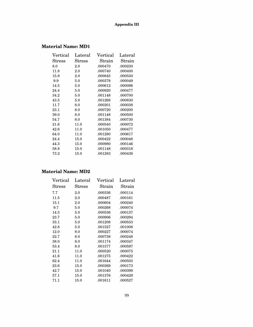
Appendix III
99
Material Name: MD1
Vertical Lateral Vertical LateralStress Stress Strain Strain8.0 2.0 .000470 .00023011.8 2.0 .000740 .00040015.9 2.0 .000845 .000550 9.9 5.0 .000378 .00004914.5 5.0 .000612 .00009624.4 5.0 .000920 .00047734.2 5.0 .001148 .00070043.5 5.0 .001268 .00083011.7 8.0 .000301 .00003823.1 8.0 .000720 .00020039.0 8.0 .001148 .00050054.7 8.0 .001384 .00073021.6 11.0 .000540 .00007242.6 11.0 .001050 .00047764.0 11.0 .001280 .00061724.4 15.0 .000422 .00004844.3 15.0 .000980 .00014658.8 15.0 .001148 .00031673.2 15.0 .001283 .000436
Material Name: MD2
Vertical Lateral Vertical LateralStress Stress Strain Strain7.7 2.0 .000336 .00011411.5 2.0 .000487 .00016115.1 2.0 .000604 .000240 9.7 5.0 .000268 .00007414.3 5.0 .000536 .00013723.7 5.0 .000906 .00029433.1 5.0 .001208 .00055342.8 5.0 .001527 .00100812.0 8.0 .000227 .00007422.7 8.0 .000738 .00024838.0 8.0 .001174 .00034753.4 8.0 .001577 .00059721.1 11.0 .000520 .00007541.6 11.0 .001275 .00042262.4 11.0 .001644 .00050323.6 15.0 .000369 .00017342.7 15.0 .001040 .00039957.1 15.0 .001376 .00042971.1 15.0 .001611 .000527

Appendix III
100
Material Name: MD3Vertical Lateral Vertical LateralStress Stress Strain Strain7.6 2.0 .000385 .00010711.9 2.0 .000544 .00011815.3 2.0 .000653 .0001669.3 5.0 .000218 .00009114.4 5.0 .000436 .00014123.5 5.0 .000812 .00024533.3 5.0 .001106 .00046242.8 5.0 .001407 .00071811.5 8.0 .000167 .00004622.6 8.0 .000616 .00017938.5 8.0 .001105 .00027854.1 8.0 .001575 .00057021.8 11.0 .000436 .00014642.2 11.0 .001122 .00032563.3 11.0 .001608 .00073223.8 15.0 .000410 .00006542.1 15.0 .000955 .00024857.6 15.0 .001306 .00043071.0 15.0 .001608 .000584