Embed Size (px)
Citation preview

NAVAL POSTGRADUATE SCHOOL MONTEREY, CALIFORNIA
THESIS
OPTIMAL SOLUTION SELECTION FOR SENSITIVITY-BASED FINITE ELEMENT MODEL UPDATING AND STRUCTURAL
DAMAGE DETECTION
by
Jay A. Renken
December, 1995
Thesis Advisor: Joshua H. Gordis
Approved for public release; distribution is unlimited.
mc W*m issPBcnsD i

DISCLAIM! NOTICE
THIS DOCUMENT IS BEST
QUALITY AVAILABLE. THE COPY
FURNISHED TO DTIC CONTAINED
A SIGNIFICANT NUMBER OF
PAGES WHICH DO NOT
REPRODUCE LEGIBLY.

REPORT DOCUMENTATION PAGE Form Approved OMB No. 0704-0188
Public reporting burden for this collection of information is estimated to average 1 hour per response, including the time for reviewing instruction, searching existing data sources, gathering and maintaining the data needed, and completing and reviewing the collection of information. Send comments regarding this burden estimate or any other aspect of this collection of information, including suggestions for reducing this burden, to Washington Headquarters Services, Directorate for Information Operations and Reports, 1215 Jefferson Davis Highway, Suite 1204, Arlington, VA 22202-4302, and to the Office of Management and Budget, Paperwork Reduction Project (0704-0188) Washington DC 20503.
1. AGENCY USE ONLY (Leave blank) 2. REPORT DATE
December 1995 3. REPORT TYPE AND DATES COVERED
Master's Thesis
4. TITLE AND SUBTITLE OPTIMAL SOLUTION SELECTION FOR SENSITIVITY-BASED FINITE ELEMENT MODEL UPDATING AND STRUCTURAL DAMAGE DETECTION
6. AUTHOR(S) Jay A. Renken
FUNDING NUMBERS
7. PERFORMING ORGANIZATION NAME(S) AND ADDRESS(ES) Naval Postgraduate School Monterey CA 93943-5000
PERFORMING ORGANIZATION REPORT NUMBER
9. SPONSORING/MONITORING AGENCY NAME(S) AND ADDRESS(ES) 10. SPONSORING/MONITORING AGENCY REPORT NUMBER
11. SUPPLEMENTARY NOTES The views expressed in this thesis are those of the author and do not reflect the official policy or position of the Department of Defense or the U.S. Government.
12a. DISTRIBUTION/AVAILABILITY STATEMENT Approved for public release; distribution is unlimited.
12b. DISTRIBUTION CODE
13. ABSTRACT (maximum 200 words)
The finite element model has become the standard way in which complex structural systems are
modeled, analyzed, and the effects of loading simulated. A new method is developed for comparing
the finite element simulation to experimental data, so the model can be validated, which is a critical
step before a model can be used to simulate the system. An optimization process for finite element
structural dynamic models utilizing sensitivity based updating is applied to the model updating and
damage detection problems. Candidate solutions are generated for the comparison of experimental
frequencies to analytical frequencies, with mode shape comparison used as the selection criteria for the
optimal solution. The method is applied to spatially complete simulations and to spatially incomplete
experimental data which includes the model validation of a simple airplane model, and the damage
localization in composite and steel beams with known installed damage.
14. SUBJECT TERMS Finite Element Model Update 15. NUMBER OF PAGES 214
16. PRICE CODE
17. SECURITY CLASSIFI- CATION OF REPORT Unclassified
18. SECURITY CLASSIFI- CATION OF THIS PAGE Unclassified
19. SECURITY CLASSIFICA- TION OF ABSTRACT Unclassified
20. LIMITATION OF ABSTRACT UL
NSN 7540-01-280-5500 Standard Form 298 (Rev. 2-89) Prescribed by ANSI Std. 239-18 298-102

11

Approved for public release; distribution is unlimited.
OPTIMAL SOLUTION SELECTION FOR SENSITIVITY-BASED FINITE ELEMENT MODEL UPDATING AND STRUCTURAL DAMAGE
DETECTION
Jay A. Renken
Lieutenant Commander, United States Navy
B.S., University of Illinois, 1983
Submitted in partial fulfillment
of the requirements for the degrees of
MASTER OF SCIENCE IN MECHANICAL ENGINEERING MECHANICAL ENGINEER
from the
Author:
Approved by:
NAVAL POSTGRADUATE SCHOOL December 1995
Joshua H. Gordis, Thesis Advisor
I Matthew D. Kelleher, Chairm Matthew D. Kelleher, Chairman
Department of Mechanical Engineering
in

IV

ABSTRACT
The finite element model has become the standard way in which complex structural
systems are modeled, analyzed, and the effects of loading simulated. A new method is
developed for comparing the finite element simulation to experimental data, so the model
can be validated, which is a critical step before a model can be used to simulate the system. An optimization process for finite element structural dynamic models utilizing sensitivity based updating is applied to the model updating and damage detection problems. Candidate solutions are generated for the comparison of experimental frequencies to analytical frequencies, with mode shape comparison used as the selection criteria for the optimal solution. The method is applied to spatially complete simulations and to spatially incomplete experimental data which includes the model validation of a simple airplane model, and the
damage localization in composite and steel beams with known installed damage.

VI

TABLE OF CONTENTS
I. INTRODUCTION 1
A. BACKGROUND 2
B. ANALYSIS METHODS 2
C. ANALYSIS APPLICATIONS 4
1. Model Updating 4
2. Damage Localization 7
II. THEORY 11
A. FREQUENCY SENSITIVITIES 11
B. ASSESSING SENSITIVITY ANALYSIS 13
C. OPTIMIZATION 14
D. OPTIMIZATION SCALING 16
E. DESIGN VARIABLE COMBINATIONS 17
F. MODAL ASSURANCE CRITERION 19
III. COMPUTER SIMULATION 21
A. BEAM MODEL UPDATING 21
1. Sensitivity Linearity Assessment 22
2. Initial Optimization Procedures 27
a. Test Case 1 - 2 Design Variables, No Scaling .... 30
b. Test Case 2 - 2 Design Variables, With Scaling .. 32
c. Test Cases 3 and 4 - Objective Function
Weighting 34
3. Advanced Optimization Procedures 36
a. Test Case 5 - Multiple Design Variables
Combinations 37
b. Test Case 6 - Prescribed Error Effects 39
Vll

c. Test Case 7 - Alternate Objective Function 40
4. Two Region Optimization 44
a. Test Case 8- 4 Design Variables 45
5. Model Updating Observations 47
B. BEAM DAMAGE LOCALIZATION 48
1. Damage Localization Process 50
2. One Inch Crack 51
a. Centered Damage - Elements 24-25 51
b. Off Center Damage - Element 40 55
3. 2.25 Inch Crack 56
a. Centered Damage - Elements 23-26 56
b. Off Center Damage - Elements 30-31 57
4. 4.5 Inch Crack 58
a. Centered Damage - Elements 22-27 58
b. Off Center Damage - Elements 5-8 59
5. 9 Inch Crack 60
a. Centered Damage - Elements 20-29 60
b. Off Center Damage - Elements 37-45 61
6. Damage Localization Observations 61
IV. EXPERIMENT 63
A. EXPERIMENTAL MEASUREMENT 63
B. SPATIALLY INCOMPLETE DATA 64
1. Extraction Method 65
2. Transformation Matrix Reduction and Expansion 66
C. MODEL UPDATING 67
1. Test Article Description 67
2. Finite Element Model Description 68
3. Model Updating Problem 69
viii

4. Optimization Process 72
5. Optimization Solution 73
6. Solution Interpretation 74
D. COMPOSITE BEAM DAMAGE LOCALIZATION 75
1. Test Article and Finite Element Model Description 75
2. Finite Element Model Update 76
3. Damage Localization 77
4. Localization Results 78
5. Solution Interpretation 80
E. STEEL BEAM DAMAGE LOCALIZATION 80
1. Test Article and Finite Element Model Description 81
2. Finite Element Model Update 82
3. Damage Localization 83
4. Solution Method 84
5. Localization Results 84
6. Simulated Experimental Damage 85
a. Frequency Substitution 87
b. Mode Shape Substitution 88
c. Frequency and Mode Shape Substitution 89
7. Solution Interpretation 90
V. CONCLUSIONS / RECOMMENDATIONS 93
A. SUMMARY 93
B. CONCLUSIONS 94
C. RECOMMENDATIONS 95
APPENDIX A. ALUMINUM BEAM SPECIFICATIONS 99
A. PHYSICAL DIMENSIONS AND PROPERTIES 99
B. DYNAMIC RESPONSE 99
ix

C. OPTIMIZATION RESULTS 102
APPENDIX B. COMPOSITE BEAM SPECIFICATIONS Ill
A. PHYSICAL DIMENSIONS AND PROPERTIES Ill
B. DYNAMIC RESPONSE 112
APPENDIX C. EXPERIMENTAL SETUP 117
APPENDIX D. AIRPLANE MODEL SPECIFICATIONS 123
A. PHYSICAL DIMENSIONS AND PROPERTIES 123
B. DYNAMIC RESPONSE 123
APPENDIX E. AIRPLANE FINITE ELEMENT MODEL 135
APPENDIX F. COMPOSITE BEAM TEST DATA 149
APPENDIX G. STEEL BEAM SPECIFICATIONS 161
A. PHYSICAL DIMENSIONS AND PROPERTIES 161
B. DYNAMIC RESPONSE 161
APPENDIX H. COMPUTER CODE 173
APPENDIX I. IDEAS CONVERSION INFORMATION 193
A. SENSITIVITY CONVERSION 193
B. MODE SHAPE NORMALIZATION AND MODAL MASSES . 194

LIST OF REFERENCES 195
INITIAL DISTRIBUTION LIST 197
XI

Xll

LIST OF FIGURES
1-1 1-2 3-1 3-2 3-3 3-4 3-5 3-6 3-7 3-8 3-9 3-10 3-11 4-1 4-2 4-3 A-l A-2 A-3 A-4 A-5 B-l B-2 B-3 B-4 B-5 B-6 B-7 B-8 B-9 B-10 C-l D-l D-2 D-3 D-4 D-5 D-6 D-7 D-8 D-9 D-10
Optimization Flow Diagram Damage Localization Flow Diagram Absolute Value of Percentage Error for 1st Natural Frequency Update . Absolute Value of Percentage Error for 2nd Natural Frequency Update Test Case 1 Solution Results , Test Case 2 Solution Results Test Case 3 Solution Results Test Case 4 Solution Results Test Case 5 Solution Results Test Case 6 Solution Results Test Case 7 Solution Results Test Case 8 Solution Results Region Expansion, 1 inch Centered Crack Analytical Model Frequency Percentage Error Airplane Model Design Variable Regions Frequency Error Comparison, Original and Updated Models Aluminum Beam Aluminum Beam, 1st Mode Shape Aluminum Beam, 2nd Mode Shape Aluminum Beam, 3rd Mode Shape Aluminum Beam, 4th Mode Shape Composite Beam Composite Beam Analytical Mode Shape 1 Composite Beam Analytical Mode Shape 2 Composite Beam Analytical Mode Shape 3 Composite Beam Analytical Mode Shape 4 Composite Beam Analytical Mode Shape 5 Composite Beam Analytical Mode Shape 6 Composite Beam Analytical Mode Shape 7 Composite Beam Analytical Mode Shape 8 Composite Beam Analytical Mode Shape 9 Experimental Setup Experimental Data Points Airplane Experimental Mode Shape 1 Airplane Experimental Mode Shape 2 Airplane Experimental Mode Shape 3 Airplane Experimental Mode Shape 4 Airplane Experimental Mode Shape 5 Airplane Experimental Mode Shape 6 Airplane Experimental Mode Shape 7 Airplane Experimental Mode Shape 8 Airplane Experimental Mode Shape 9
5 8 24 24 31 33 35 35 38 40 42 46 54 70 71 74 99 100 100 101 101 111 112 113 113 114 114 115 115 116 116 117 124 125 126 127 128 129 130 131 132 133
Xlll

D-l 1 Airplane Experimental Mode Shape 10 134 E-l Airplane Finite Element Model 136 E-2 Airplane Analytical Mode Shape 1 137 E-3 Airplane Analytical Mode Shape 2 138 E-4 Airplane Analytical Mode Shape 3 139 E-5 Airplane Analytical Mode Shape 4 140 E-6 Airplane Analytical Mode Shape 5 141 E-7 Airplane Analytical Mode Shape 6 142 E-8 Airplane Analytical Mode Shape 7 143 E-9 Airplane Analytical Mode Shape 8 144 E-10 Airplane Analytical Mode Shape 9 145 E-l 1 Airplane Analytical Mode Shape 10 146 F-l Composite Beam Excitation Points 150 F-2 Composite Beam Experimental Mode Shape 1 151 F-3 Composite Beam Experimental Mode Shape 2 152 F-4 Composite Beam Experimental Mode Shape 3 153 F-5 Composite Beam Experimental Mode Shape 4 154 F-6 Composite Beam Experimental Mode Shape 5 155 F-7 Composite Beam Experimental Mode Shape 6 156 F-8 Composite Beam Experimental Mode Shape 7 157 F-9 Composite Beam Experimental Mode Shape 8 158 F-10 Composite Beam Experimental Mode Shape 9 159 G-l Steel Beam 161 G-2 Steel Beam Excitation Points 163 G-3 Steel Beam Experimental Mode Shape 1 164 G-4 Steel Beam Experimental Mode Shape 2 165 G-5 Steel Beam Experimental Mode Shape 3 166 G-6 Steel Beam Experimental Mode Shape 4 167 G-7 Steel Beam Experimental Mode Shape 5 168 G-8 Steel Beam Experimental Mode Shape 6 169 G-9 Steel Beam Experimental Mode Shape 7 170 G-10 Steel Beam Experimental Mode Shape 8 171 G-l 1 Steel Beam Experimental Mode Shape 9 172
XIV

LIST OF TABLES
2-1 2-Level Factorial Test, "After [Ref. 6: p. 58]" 18 3-1 Cauchy Ratio Equivalent Calculated Values 26 3-2 Damage Localization Results, First Iteration, 1 inch Crack,
Elements 24-25 52 3-3 Damage Localization Results, Second Iteration, 1 inch Crack,
Elements 24-25 53 3-4 Damage Localization Results, Third Iteration, 1 inch Crack,
Elements 24-25 53 3-5 Damage Localization Results, 1 inch Off Center Crack 55 3-6 Damage Localization Results, 2.25 inch Centered Crack 56 3-7 Damage Localization Results, Fourth Iteration, 2.25 inch Centered 57
Crack 3-8 Damage Localization Results, 2.25 inch Off Center Crack 57 3-9 Damage Localization Results, 4.5 inch Centered Crack 58 3-10 Damage Localization Results, 4.5 inch Off Center Crack 59 3-11 Damage Localization Results, 9 inch Centered Crack 60 3-12 Damage Localization Results, 9 inch Off Center Crack 61 4-1 Airplane Model Dynamic Response 69 4-2 Composite Beam Update Data 77 4-3 Composite Beam Damage Search Results, Extraction Method 78 4-4 Composite Beam Damage Search Results, Static Reduction 79 4-5 Composite Beam Damage Search Results, Static Expansion 79 4-6 Composite Beam Damage Search Results, IRS Reduction 80 4-7 Composite Beam Damage Search Results, IRS Expansion 80 4-8 Steel Beam Update Data 83 4-9 Steel Beam Damage Search Results, Extraction Method 85 4-10 Simulated Experimental Data Comparison 86 4-11 Steel Beam Damage Search Results, Simulated Experimental Data 86 4-12 Experimental Data Substitution Results 87 A-l Test Case 1 Numerical Results 102 A-2 Test Case 2 Numerical Results 103 A-3 Test Case 3 Numerical Results 104 A-4 Test Case 4 Numerical Results 105 A-5 Test Case 5 Numerical Results 106 A-6 Test Case 6 Numerical Results 107 A-7 Test Case 7 Numerical Results 108 A-8 Test Case 8 Numerical Results 109 D-l Airplane Model Dimensions 123 E-l Airplane Update Frequency Comparison 147
XV

XVI

I. INTRODUCTION
A. BACKGROUND
Finite element models are widely used to predict the response characteristics of
complex structures in the area of structural dynamics. The models can be very complex
and use large numbers of degrees of freedom so that the desired level of accuracy will be
achieved. However, the construction of the models can be an inexact science. Variations
such as non-homogenity in physical properties within structures, difficulties in
determining the stiffness of different types of structural joints, and the inability for the
solution of a finite degree of freedom model to converge to the exact solution of an
infinite degree of freedom system make the task of constructing an accurate model
daunting.
In view of these difficulties with finite element models, methods of model
updating to improve model correlation with tests have been explored [Ref. 1-3]. Methods
for model updating are based on the comparison of analytical data from finite element
models to that of experimentally obtained data from the structures being modeled.
Dynamic response parameters used for this comparison are the natural frequencies of
vibration, corresponding mode shapes, and damping behavior. The real question becomes
how is the dynamic response information fed back into the model to make corrections?
There are two major difficulties with updating an analytical model. The first difficulty is
that when dealing with a complex model there are large numbers of variables that can be
adjusted resulting in a very large search domain. Related to this problem with the search
process is that there are an infinite number of design variable combination changes that

will result in a mathematically correct yet non-unique solution for the model system. The
second difficulty is that the solution time to re-solve the eigenproblem for complex
models can be quite large and very expensive, which limits the number of variable change
combinations that can be investigated in a cost effective manner. With these difficulties in
mind it is imperative that a search routine to update models will minimize iterations and
therefore cost, as well as provide verifiable and accurate results.
Once a finite element model has been updated it is used to accurately predict the
dynamic response characteristics of the modeled structure and to investigate the effect of
design changes. This allows non-destructive testing of the structure to various simulated
loads ensuring adequate strength or performance of the structure. Another application of
the updated model is in the area of localizing structural damage in a structure. Measured
dynamic response parameters of a structure that is believed to be damaged are compared
to the updated model. The search process used to update the model is then applied to
determine where differences between analysis and test occurred, thereby localizing the
probable area of damage.
B. ANALYSIS METHODS
Dynamic response parameters are generated for the analytical model and the
actual structure. The parameters experimentally determined from the actual structure are
the natural frequencies of the structure and the corresponding mode shapes. The
parameters for the initial analytical model are the natural frequencies and the associated
frequency sensitivities. Finite element model sensitivities are the first derivative of the
eigen problem solution set with respect to the design variables under consideration.

Frequency sensitivities are the basis for a linear approximation to compute the change in
the natural frequencies of a model based on a change in a given design variable. This
method of frequency updating greatly reduces the computational time required to
calculate the results of a change to large finite element models by eliminating the need to
re-solve the eigenproblem for each iteration. This process of frequency updating has been
used extensively for model updating and is discussed further in references (1) through (3).
To search the solution domain for prospective solutions, a constrained
optimization routine is employed. Optimization theory and techniques are discussed
further in reference (4). The optimization routine employed searches for the minimum
value of an objective function which is constructed to minimize the differences between
the analytical model parameters and the experimental data. This organized approach of
searching for the optimal combination of design variables minimizes the number of
combinations that are investigated thereby reducing the computational requirements of
this process.
The real difficulty to this method of correcting a finite element model is to
determine which candidate solution most closely matches the experimental data. Multiple
combinations of design variable changes can result in the same changes to the natural
frequencies of the model so the accuracy of the frequencies is not the only evaluation
factor. An improved method of solution evaluation is to determine the effects on the
analytical mode shapes and compare them to the experimental mode shapes. This
comparison of mode shapes is called the Modal Assurance Criterion (MAC) and is
discussed in reference (5). The MAC is a measure of how closely two mode shapes

coincide. The candidate solution with a MAC value most close to one when compared to
the experimental data most closely resembles the experimental case and is selected as the
optimal solution.
C. ANALYSIS APPLICATIONS
There are two applications of this optimal solution search procedure using finite
element model sensitivities and frequency differences. The first application of the
procedure is updating the system finite element model. Model updating correlates the
baseline model for use for system computations. The second procedure involves damage
localization using a previously updated model. There are numerous non-destructive
methods for testing structures but most are limited to surface defects. By comparing the
change in the vibrational characteristics of a validated system as well as comparing the
mode shapes the finite element model can be used as a damage localization system for
internal structure defects.
1. Model Updating
Model updating is imperative to verify the accuracy of a finite element model. The
method that was chosen to update the model was an optimization search utilizing
sensitivity based frequency updates. Figure 1-1 is a flow diagram of the updating process.
This method is similar to those as discussed in references (1) to (3) with differences in
design variable scaling and choice of objective function. The initial step is to develop the
finite element model of the structure to generate the analytical frequencies and design
variable sensitivities. The actual structure is also tested to provide the experimental data.
The objective function is then selected. The objective function is the equation that the

Develop FEM and Sensitivities Test Actual Structure
Select Objective Function
Select Design Variables
Enter Optimization Loop with Different Combinations of Design Variables
Scale Design Variables if Necessary
Solve Optimization Problem
Update FEM Frequencies and mode Shapes for Solution Evaluation
Calculate MAC
Repeat Through Design Variable Combinations
Select Optimal Solution
Figure 1-1 Optimization Flow Diagram

optimization process will minimize. The parameters chosen for the objective function can
vary. In reference (1) the summation of the percentage difference in the system
frequencies and the absolute change in the design variables were chosen. In reference (2),
differences in the frequencies, the mode shapes and the static deflection were chosen. For
this thesis two objective functions were investigated. The first was a scaled sum of the
percentage difference in the frequencies added to the sum of the percentage change of the
design variables during the domain search. The second type of objective function is the
sum of the change in design variables during the domain search constrained by
maintaining the difference in the analytical and experimental frequencies below a chosen
tolerance.
The design variables are chosen based on the specifics of the model and the
structure. These could be material property values or assumed values of joint stiffness or
any other variable which was chosen with some level of uncertainty. At this point the
optimization loop is entered. Combinations of the design variables are chosen so that all
possible combinations are investigated. These type of search is discussed in reference (6).
This type of search pattern will result in 2n-l iterations, where n is the number of design
variables chosen. This drives the use of less design variables to minimize computation
time.
If the design variables are of differing magnitudes they should be scaled to be the
same size. This will reduce the chance that a single variable will dominate the
optimization process. The scaled design variables are used with the frequency
sensitivities to update the objective function. The optimization process uses a 1st order

search routine to find the minimum objective function value within the search domain.
The optimized design variables are then fed back into a routine to solve the eigenproblem
generating the natural frequencies and mode shapes for this variable combination. The
mode shapes are compared to the experimental data by computing the MAC and are
summed for the modes of interest. This process is repeated for all the combinations of the
design variables. The combination of design variables with the highest MAC value is
chosen as the optimal solution.
2. Damage Localization
The process chosen for damage localization utilizes the same basic optimization
routine as model updating with a different search logic. This method is based on the
premise that any sub-surface defects in the material will be manifested in a finite element
model as a reduction in the stiffness of the structure. It was assumed that there would be
no mass loss for this situation. Figure 1-2 is a flow diagram of the damage localization
process. It differs from the procedures discussed in references (7) through (10) in the
search methodology and evaluation methods. The process still begins with the
comparison of the analytical data and the experimental data. The objective function is the
same as in the validation process.
The major difference between the model updating process and the damage
location process is that the design variables considered are the element stiffnesses within
designated search regions. The search logic is that a selected search region is divided into
sub-regions. The stiffness of a sub-region is optimized as if it had suffered a reduction
resulting in the experimentally observed frequency shifts for the damaged case. The

Develop FEM and Sensitivities From Optimized Model
Test Damaged Structure
Select Objective Function
Divide Structure into Regions
Enter Optimization Loop
For a Search Region
Solve Optimization Problem
Update FEM Mode Shapes for Evaluation
Calculate MAC
Repeat Through Each Sub-Region and Overall Region
Select Most Probable Sub-Region
Repeat Search within Sub-Region
Select Optimal Solution
Figure 1-2 Damage Localization Flow Diagram

reduced stiffness for that sub-region is fed back into the finite element model to generate
assumed damage mode shapes. These mode shapes are then compared with the
experimental mode shapes with the MAC. This process is repeated for all of the search
sub-regions as well as the overall region of the search. The sub-region with the highest
summed MAC value is evaluated as the most probable area of damage if the MAC value
does not exceed that of the entire region. The selection of the most probable sub-region is
then used to start another search iteration with the smaller region. This process is repeated
until the damage is localized to a single element of the analytical model or the search
region is evaluated as more probable then any single sub-region. At this point the most
probable area of damage is selected.

10

II. THEORY
A. FREQUENCY SENSITIVITIES
A typical dynamic response finite element model is a method to mathematically
model the response characteristics of a structure. The properties of the structure are
reduced to the eigenvalue problem for dynamic structural response as given by:
[K][O>]-[M][<D][A] = 0 (2.1)
where [K] is the system stiffness matrix, [M] is the system mass matrix, [A] is the
eigenvalue matrix, and [O] is the eigenvector matrix. [K] and [M] are defined by the
physical properties of the system including the physical dimensions, mass density and the
Young's modulus of the materials in the structure. The stiffness and mass matrices are
nxn in size where n is the number of degrees of freedom within the model. [A] is a nxn
diagonal matrix which contains the system eigenvalues. [<J>] is a nxn matrix whose
columns define the mode shapes of the system. The natural frequencies of the system are
computed from the eignvalue matrix. The ith natural frequency of the system, in Hertz, is
calculated as follows:
G*=A (2-2)
f;=^ (2-3)
where Xi is the ith diagonal term of the eigenvalue matrix. Equation (2.1) can be
rearranged and still holds for each individual mode as shown for the ith mode in the
following:
[[K]-A1[M]]{<|)i}=0 (2.4)
11

Now consider a change in the kth design variable, Vk, which may affect both [K]
and [M]. Differentiating Equation (2.4) with respect to vk results in:
3K
3v, 3v. [M]-\ 3M
3v, ^J+IM-^IM]]^ =0 (2.5)
Equation (2.5) is then premultiplied by {^}T, the transpose of the ith mode shape,
resulting in equation (2.6).
MT 3K
3v,
9M
L3vk. {♦,}+MT[M-Wfj4 = 0 (2-6)
Because of the orthogonality of eigenvectors Equation (2.7) through Equation (2.9) hold:
[K] = [K]T
[M] = [M]T
{^}T[[K]-^[M]] = 0
(2.7)
(2.8)
(2.9)
Substituting Equation (2.9) into Equation (2.6) eliminates the second term of the left hand
side. Rearranging terms yields Equation (2.10):
3^ M1 3K
3v, -X,
3M
3v, h} (2.10)
If mass normalized mode shapes are utilized the denominator of Equation (2.10) is equal
to 1 reducing Equation (2.10) to:
M 3K
3v„. ■k
3M
3v,_ (♦.} (2.11)
12

Equation (2.11) is then used to calculate the sensitivity matrix, [T], for the analytical
model. [T] is a nxm matrix where n is the number of modes used and m is the number of
design variables considered. The sensitivity matrix is used to approximate the frequency
shift of the analytical system within the optimization loop for small changes in the design
variables with Equation (2.12):
{AX}=[T]{Avk} (2.12)
Where A symbolizes small changes in the eigenvalues and the design variables.
B. ASSESSING SENSITIVITY ANALYSIS
Because Equation (2.12) is a linear approximation for a non-linear situation it is
only valid for small changes in the vicinity of the system eigenvalues and original design
variable values. A method to assess the applicability of the sensitivity approximation is
derived in detail in reference (11). The method utilizes second-order sensitivities to
evaluate if the use of first order sensitivities are appropriate. "The method is based on the
use of a truncated Taylor Series extrapolation" [Ref. 11: p. 136] and "the Cauchy
condition for the convergence of a general power series" [Ref. 11: p. 136]. "Analogy to
the Cauchy ratio test suggests that the convergence of the Taylor series is likely to depend
on the ratio" [Ref. 11: p. 136]:
Av 1fe}T ~9K"
-\ 3M"
UvJ. M
™*M 3K
Uk_ -\ 3M
LavJ. M 06; (2.13)
with
13

MT 1>J -
3MT
UvJJ fe} «ij=-
(^) (2.14)
Where i indicates the mode of interest, j indicates all other modes, and k indicates the
design variable of interest. The determination of acceptability of the first order sensitivity
approximation is based on the value of j^. "If TJJ is much less than one the approximation
should be accurate" [Ref. 10: p. 136].
C. OPTIMIZATION
"The purpose of numerical optimization is to aid in rationally searching for the
best design to minimize a function of the design variables to satisfy constraints" [Ref. 4:
p. 1]. In this instance the purpose is to match the dynamic response of a finite element
model to that of the experimental response of the system of interest. "The general
problem statement for a non-linear constrained optimization problem is" [Ref. 4: p. 9]:
Minimize: F(X) Objective Function (2.15)
Subject to:
gj(X)<0 j = l,m
hk(X) = 0 k=l,p
Xi'<Xi<XiU i=l,n
X,
Inequality Constraints
Equality Constraints
Side Constraints
(2.16)
(2.17)
(2.18)
where X =
X2
X,
x„
Design Variables
14

The vector X is the vector of design variables. The constraint equations are used to bound
possible solution combinations to meet the requirements of the given situation.
Most optimization algorithms require that an initial set of design variables, X°, be
specified. Beginning from this starting point, the design is updated iteratively. This
process can be written as:
Xq = Xq4 + aSq (2.19)
where q is the iteration number and S is a vector search direction in the design space.
"The scalar quantity a defines the distance that we wish to move in direction S" [Ref. 4:
p. 10]. The updated values of X are used to calculate the value of the objective function
for each iteration. The search direction is chosen to decrease the value of the objective
function while staying within the constraints of the system. The process continues until
the objective function converges to a local minimum and the optimal solution is
localized.
There are many methods to choose the search direction, S The search direction
selected for this thesis is the steepest descent method. In the steepest descent method the
search direction is taken as the negative of the gradient of the objective function. That is
at iteration q:
Sq = - VF(Xq) (2.20)
"This Sq vector is used in Equation (2.19) to perform a one-dimensional search" [Ref. 4:
p. 88].
15

D. OPTIMIZATION SCALING
For the model optimization problem the design variables being considered can
have greatly different magnitudes. To ensure that each design variable has the same effect
on the optimization process it is beneficial to scale the design variables. "Scaling has the
effect of putting each variable on the same basis in the sense that a 1 percent change has
roughly the same meaning for each variable" [Ref. 4: p. 100]. The method of scaling
chosen was to scale variables to the value of the smallest design variable. This results in
the construction of a nxn diagonal scaling matrix, Sc. The kth diagonal term of the scaling
matrix is X^/X^. Scaled design variables can then be calculated with the following:
|X}=[SC]{X} (2.21)
where the tilde symbolizes scaled values. Rearranging Equation (2.21) results in:
{X}=[SC]_1{X} (2.22)
Applying the scaling logic of Equation (2.22) to the particular function stated in Equation
(2.12) results in the following:
{AX}=[T][Sc]_,{Avk} (2.23)
Combining the sensitivity matrix and the inverted scaling matrix results in the scaled
change in frequency function used in the objective function for the scaled optimization
problem:
{A?i}=[f]{Avk} (2.24)
16

E. DESIGN VARIABLE COMBINATIONS
When conducting an experiment to see how design variables effect a given
function, "a logical way to manage the experiment is to change one design variable at a
time, which is called the classical one-factor-at-a-time (1-F.A.A.T.) technique" [Ref. 6: p.
51]. This method, although orderly and thorough, does not take into account any
interrelation between design variables, or allow for multiple factors to be considered
together. Another approach to this experiment is to examine k factors, in n observations,
with each factor at two levels. "This approach is called the 2-level factorial design" [Ref.
6: p. 54]. By two levels it is meant that a particular factor is either considered at a low
level or a high level for each observation. "The total number of observations in such an
experiment is determined by taking the number of levels (2) to the power of the number
of factors (k) such that n = 2k" [Ref. 6: p. 54]. "In this design we look at all possible
combinations of the two level design variables" [Ref. 6: p. 54].
In the context of this thesis there are minor modifications to the 2-level factorial
design. The first is that the low level of the design variable means that it is not adjusted.
The high level of the design variable means that it is adjusted. To symbolize whether a
design variable is considered or not a binary notation is used. A 0 means the design
variable is not considered while a 1 indicates that the design variable is considered. With
these symbols a table can be constructed to describe the design variable combinations for
the experiment. Table 2-1 is an example of how a experiment would be set up for three
design variables. Three design variables for two levels would result in 2 or 8
17

Observation Design Variable Design Variable Desig n Variable
(1) (2) (3)
1 0 0 0 2 1 0 0 3 0 1 0 4 1 1 0 5 0 0 1 6 1 0 1 7 0 1 1 8 1 1 1
Table 2-1 2-Level Factorial Test, "After [Ref. 6: p. 58]"
observations. Some observations on the 2-level factorial test table design from reference
(6): p. 57 are included:
"Note the pattern in the columns in Table 2-1. The first column varies the O's and l's alternately, while the second column varies them in pairs and third in fours. In general, we can reduce the pattern of the digits in any column to a formula: The number of like digits in a set = 2n~ where n is the column in the matrix.
forn=l,21"1 = 2°=l for n =2, 22"1 = 21 = 2 for n =3, 23"1 = 22 = 4 for n =4, 24"1 = 23 = 8 , etc.
The convention of alternating O's and l's produces an order in the experimental design, which is useful in the design and analysis. It is called Yates order after the British statistician."
In the context of the finite element updating problem, the first combination listed in Table
2-1 is the original model and as such is not considered. Therefore the number of design
variable combinations to be considered for model updating is 2 -1 with k being the
number of design variables of interest.
18

F. MODAL ASSURANCE CRITERION
"The Modal Assurance Criterion (MAC) is a scalar constant relating the causal
relationship between two modal vectors" [Ref. 5: p. 113]. For this thesis the MAC is used
as a means to compare analytically and experimentally obtained vibrational mode shapes.
The MAC will have a value between 0 and 1. A value of 0 indicates that the two modal
vectors are not consistent while a value of 1 indicates the modal vectors are consistent.
The method of calculating the MAC for comparing the ith mode of the analytical (a)
system to the ith mode of the experimental (x) system is:
MAC = (2.25) |M%|fc}%|
The individual MAC values for each vibrational mode of interest are then summed to
provide a scalar "rating" of the solution. The iteration with the highest summed MAC
rating is then selected as the optimal solution.
The following chapters will demonstrate the application of these theories.
Optimization theory with scaling will be applied to both model updating and damage
localization based on sensitivity updating of the finite element model. The applicability of
the sensitivity updates will be evaluated with the Cauchy ratio. The design variable
combinations are chosen with the 2-level factorial method. The results of the search
iterations will be evaluated with the MAC value.
19

20

III. COMPUTER SIMULATIONS
The investigation of model updating and damage localization was initially
conducted with computer simulations. A baseline finite element model was created to be
used as the analytical model. The baseline model was then modified by making changes
to specific model parameters, yielding a simulated experimental model with known
differences in the design variables. By comparing the baseline model and the simulated
experimental model the operation of the optimization and localization processes could be
studied and verified. The types of models, design variables modified, and the procedures
for the simulations will be discussed in further detail in this chapter.
A. BEAM MODEL UPDATING
The initial process to be examined is model updating. In order to determine the
size of design variable changes for which frequency sensitivity calculations are
appropriate and to verify optimization processes a simple finite element model was
utilized. This baseline model was constructed for an aluminum beam with damping
neglected to simplify the model. This model considered two degrees of freedom at each
node, one translation and one rotation, and contained eight elements and nine nodes. The
boundary conditions for the test cases was fixed-free, that is the left end of the beam was
clamped. The material was assumed to have homogenous physical properties. Specific
beam data is included in Appendix A.
In the simple beam model, two model parameters were chosen to be manipulated
as the design variables for the optimization investigation. The design variables chosen
were the Young's modulus and the mass density for the entire beam. The optimization
21

process is developed to determine what set of changes to the design variables in the finite
element model would result in an "updated" analytical model matching the dynamic
response of the simulated experimental model. The values of the two design variables for
the baseline finite element model will be referred to as the original values of the design
variables and the known changes to the design variables will be referred to as the design
variable errors. The original values of the design variable were either reduced, held
constant, or increased, in all possible combinations, to generate the simulated
experimental data. For two design variables, examined at three levels, there are 32 or nine
possible combinations. The combination with no changes to either design variable is
trivial, so eight different design variable error combinations were investigated. For
example, one error combination was a decrease in density while modulus was held
constant. The use of different error combinations was to determine if the type of errors in
the design variables affected the optimization solution. The design variable errors for the
simulated experimental models were at least five percent of the original values to ensure
that a noticeable difference in the dynamic response parameters was observed. The
different aspects of the optimization process were investigated with multiple test cases.
Each test case examined a particular solution aspect and consisted of eight trials, one for
each of the design variable error combinations. This allowed the isolation of the effects
for the items changed from test case to test case.
1. Sensitivity Linearity Assessment
The first and foremost issue which must be validated in the optimization process
is the sensitivity-based update of the finite element model. The sensitivity matrix is used
22

to approximate the change to the natural frequencies of the analytical system based on a
change to designated design variables. The relation for the frequency change was
identified in Equation (2.12). The updated analytical natural frequencies are computed as
shown in Equation (3.1). Note that the second term in the right hand side is the frequency
change as identified in Equation (2.12).
{fu
a}={fa}+[T]{ADV} (3.1)
where {f} indicates the system natural frequencies and DV represents design variables.
This approximation for the updated analytical natural frequencies is used in the numerical
optimization process to evaluate possible design variable values. The purpose of using
this approximation is to reduce the computational time to accomplish the optimization. If
the approximation was not used, the numerical optimization routine would have to re-
solve the eigenproblem for every iteration, increasing the computational time required to
solve the problem. With this in mind, it is imperative that the linearity of the sensitivity-
update be assessed to ensure that it is accurate within the solution domain.
The range of validity for the frequency sensitivity-update approximation was
assessed for the aluminum beam test model in 2 fashions both of which will be discussed
in following sections. The first method was a direct comparison of the updated natural
frequencies calculated from Equation (3.1) to that of the eigenproblem re-solve for a
given set of errors to the design variables. The design variables were varied up to plus or
minus 10 percent from the original values in the finite element model. Figure 3-1 and
Figure 3-2 are plots of the absolute value of percentage error between the eigenproblem
re-solve and the sensitivity based frequency update for the first two natural frequencies of
23

Error for Sensitivity update for 1 st Natural Frequency
% Change in Modulus -10 -10 % Change in Density
Figure 3-1 Absolute Value of Percentage Error for 1st Natural Frequency Update
Error for Sensitivity update for 2nd Natural Frequency
% Change in Modulus -10 -10 % Change in Density
Figure 3-2 Absolute Value of Percentage Error for 2nd Natural Frequency Update
24

the beam versus the percentage changes to the design variables. Both cases have a
maximum error of approximately one percent. An item to notice in the figures is that the
error is at the highest level when the design variables are adjusted in the opposite fashion.
This is because the changes in design variables have opposite effects on the system
frequencies. For example, when the modulus is increased the frequencies increase, and
when the density increases the frequencies decrease. Therefore when the design variables
are shifted in opposite directions, one positive and one negative, the overall change to the
natural frequencies is larger in magnitude and the corresponding error is larger.
Conversely when the design variables are shifted in the same direction, either both
positive or both negative, the overall change to the natural frequencies is smaller because
the changes cancel and the corresponding error is also smaller. This indicates that the
approximation error is based more on the magnitude of the change to the natural
frequencies themselves as opposed to the magnitude of the changes to the design
variables. The error levels of approximately 1 percent calculated by direct comparison of
frequencies is considered acceptable for the optimization procedure.
The second method of verifying the acceptability of the sensitivity updating
approximation was to calculate the Cauchy ratio equivalent for the model. This ratio was
defined in Equation (2.13) and Equation (2.14) included in Chapter II on page 13. The
ratio uses the magnitude of the second term in a Taylor series expansion to determine if
using the first term alone is a valid approximation This ratio is computed for a specific
design variable change in the model, and for all of the natural frequencies of interest. The
acceptability measure for this method is if the ratio has a value much less than one. This
25

ratio was calculated here for the first two natural frequencies and up to 20 percent
changes in the density and modulus. This method of assessment does not take into
consideration a combination of changes to both design variables simultaneously. The
single largest calculated ratio values are included as Table 3-1. The ratio exceeds 0.1
when the mass density changes by eight percent and when the modulus changes by 12
percent, both for the second natural frequency. The question with this validation method
is what value of the ratio actually indicates that the accuracy limits have been exceeded?
Reference (11) only refers to a value of much less than one. Without a well defined
definition of an acceptable value the results of this method of assessment are open to
interpretation.
1st Frequency 2nd Frequency Percent Mass Modulus Mass Modulus Change Density Density
1 0.0083 0.0072 0.013 0.0091 2 0.017 0.014 0.026 0.018 3 0.022 0.025 0.027 0.039 4 0.033 0.029 0.052 0.036 5 0.041 0.036 0.064 0.045 6 0.050 0.043 0.077 0.054 7 0.058 0.070 0.090 0.064 8 0.066 0.058 0.103 0.073 9 0.074 0.065 0.115 0.082 10 0.083 0.072 0.130 0.091 11 0.091 0.080 0.142 0.099 12 0.099 0.086 0.155 0.109
Table 3-1 Cauchy Ratio Equivalent Calculated Values
Based on the results of the numerical linearity assessment ("Method 1", above),
that up to a 10 percent change in either or both of the design variables is acceptable, the
26
maximum ratio value for the 10 percent shift is chosen as the acceptable ratio value. This
value is 0.13. In view of the two methods of evaluating the sensitivity updating
approximation, the error of the approximation is at an acceptable level within a limit of
10 percent change to either or both design variables.
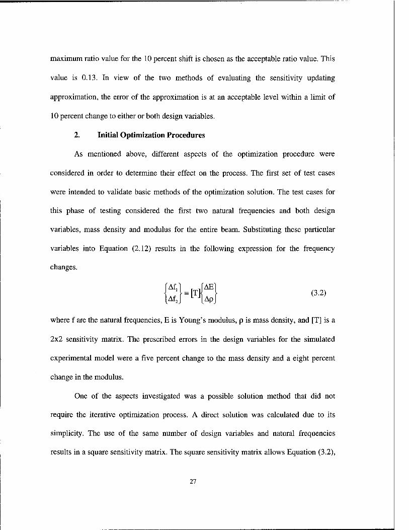
2. Initial Optimization Procedures
As mentioned above, different aspects of the optimization procedure were
considered in order to determine their effect on the process. The first set of test cases
were intended to validate basic methods of the optimization solution. The test cases for
this phase of testing considered the first two natural frequencies and both design
variables, mass density and modulus for the entire beam. Substituting these particular
variables into Equation (2.12) results in the following expression for the frequency
changes.
where f are the natural frequencies, E is Young's modulus, p is mass density, and [T] is a
2x2 sensitivity matrix. The prescribed errors in the design variables for the simulated
experimental model were a five percent change to the mass density and a eight percent
change in the modulus.
One of the aspects investigated was a possible solution method that did not
require the iterative optimization process. A direct solution was calculated due to its
simplicity. The use of the same number of design variables and natural frequencies
results in a square sensitivity matrix. The square sensitivity matrix allows Equation (3.2),
27

to be solved directly by premultiplying both sides of the equation by the inverse of the
sensitivity matrix resulting in Equation (3.3):
fAEl
■w|S A , ,-, ,.,, (3.3) API
Although this method is quick and mathematically correct, in this instance the solution
has no physical significance. That is the design variable errors calculated from this
solution method are of a significantly different magnitude than the known error values.
This was true whether the design variables were scaled or not.
Therefore the primary solution method considered was a constrained optimization
routine, as defined as in Equations (2.15) through (2.18) in Chapter II on page 14. The
purpose of the optimization routine is to locate the minimum value of an objective
function subject to imposed constraints. The process begins with a start point within the
solution domain and then uses an iterative search logic to numerically converge to a
solution. Some specifics of the optimization process can be modified to alter the results of
the search. Some items which were considered include:
• Design variable scaling
• Alternate objective functions
• Objective function scaling
• Solution constraints
• Iteration start point
The specifics of these items will be addressed in the following paragraphs.
28

One of the areas for evaluation is whether design variables should be scaled or
not. Scaling can improve the performance of the optimization routine by modifying the
problem so that the design variables are of similar magnitudes. For this beam case the
mass density and modulus differ in magnitude by a factor of 1011 so scaling may be
beneficial. Design variable scaling is investigated in Test Cases 1 and 2.
Another item to be investigated is the objective function. The objective function
used for initial optimization evaluation is of the form:
n fx — fa m ADV OF = A*t^^ + B*y^äL (3.4)
£? fi" 6 DVk
where n is the number of frequencies of interest, m is the number of design variables, and
A and B are scalar multipliers used as weighting factors in the objective function. The
analytical frequencies in Equation (3.4) are computed using the current state variables and
Equation (3.1), i.e. at each iteration of the optimization process, the analytical frequencies
are updated to determine the effect of possible design changes. This process will decrease
the difference between the experimental and updated analytical frequencies until
convergence to the minimum value of the objective function is obtained. The
optimization routine will return the design variable changes required such that the finite
element model frequencies will match the experimental frequency data. These design
variable changes are used to calculate the value of optimum design variables by adding
the changes to the original design variable values. The weighting factors, A and B, are to
enhance the effect of one term versus the other in the objective function and can be
altered to determine the effect on the optimization process of either term. Weighting of
29

the objective function terms is investigated in Test Cases 3 and 4. The only constraint
imposed at this stage was a limit of 10 percent change from the original design variable
values during the search iterations. The starting point values to begin the iterative search
were the original design variable values for all of the trials within each test case.
a. Test Case 1-2 Design Variables, No Scaling
The scalar multipliers in the objective function for this case were A = 1
and B =1. There was no scaling of the design variables. The results for Test Case 1 are
included numerically in Appendix A as Table A-l and graphically in Figure 3-3. The axes
for the plot are the percentage changes in the two design variables from the original
values of the finite element model. The set of points labeled as "Prescribed" are the eight
combinations of known design variable errors that comprise the simulated experimental
trials. The set of points labeled as "Solution" are the changes to the original design
variable values that were returned as the optimized solution by the optimization routine.
Lines connect the data point of a known error to the data point of the corresponding
optimization solution. The distance between the two data points is a measure of the
accuracy of the solution. The shorter the distance the better the solution matched the
known error condition. If a solution was within 2.5 percent of the known error for both
design variables is was judged as reasonable and noted with a ellipse enclosing both the
error data point and the solution data point. The start point for all of the trials was at the
original design variable values and is plotted at the origin of the axes.
Only two of the eight solutions are within a reasonable tolerance from the
known error values. These are not acceptable results. As shown in Figure 3-3 all of the
30

Test Case 1
3 T3 O s v D> c (0
JC Ü 0> Bl (0 *■"
c a> ü k. a> a.
-46-
-40-
« Prescribed
■ Solution
• Start Point
Percentage Change Density
Figure 3-3 Test Case 1 Solution Results
solutions lie on the horizontal line corresponding to the zero value of the vertical axis.
This indicates that the modulus was not altered by any significant amount for any of the
trials. The optimization routine minimized the frequency differences between the
analytical and experimental models by only manipulating the mass density of the beam.
This is probably due to the large difference in magnitudes between the two design
variables.
The results from Test Case 1 indicate the need to scale the design variables
to equalize their effect on the design optimization process. The optimization process will
not operate correctly for this situation when the design variables are greatly different in
31
magnitude. A method to correct this deficiency will be addressed in the following test
case.
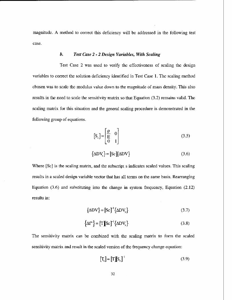
b. Test Case 2-2 Design Variables, With Scaling
Test Case 2 was used to verify the effectiveness of scaling the design
variables to correct the solution deficiency identified in Test Case 1. The scaling method
chosen was to scale the modulus value down to the magnitude of mass density. This also
results in the need to scale the sensitivity matrix so that Equation (3.2) remains valid. The
scaling matrix for this situation and the general scaling procedure is demonstrated in the
following group of equations.
[£ n [SJ= E (3-5)
0 1
{ADVs}=[Sc]{ADV} (3.6)
Where [Sc] is the scaling matrix, and the subscript s indicates scaled values. This scaling
results in a scaled design variable vector that has all terms on the same basis. Rearranging
Equation (3.6) and substituting into the change in system frequency, Equation (2.12)
results in:
{ADV} = [Sc]~'{ADVs} (3.7)
{Afa}=[TlScf{ADVs} (3.8)
The sensitivity matrix can be combined with the scaling matrix to form the scaled
sensitivity matrix and result in the scaled version of the frequency change equation:
[TsHTjSj1 (3-9)
32

{Afa}=[Ts]{ADVs} (3.10)
Equation (3.10) is then used for frequency updating for the scaled design variable
problem in Equation (3.1). This scaling logic is valid for other cases and can be applied
for larger design variable vectors by increasing the number of terms in the scaling matrix.
For Test Case 2 the scalar multipliers in the objective function were the
same as for Test Case 1. The results for Test Case 2 are included numerically in
Appendix A as Table A-2 and graphically in Figure 3-4.
Test Case 2
-43-
-40-
» Prescribed
■ Solution
• Start Point
Percentage Change Density
Figure 3-4 Test Case 2 Solution Results
The results for Test Case 2 show improvement over the results for Test
Case 1. Four of the eight trials yielded reasonable solutions, but the overall accuracy is
still not acceptable. Scaling of the design variables and the sensitivity matrix was
33

effective in that it allowed both design variables to be shifted during optimization. The
modulus was shifted by as much as five percent for one of the trials demonstrating that
modulus had been manipulated during the optimization process. Although scaling
allowed both design variables to be manipulated, this in itself did not guarantee that all of
the trials in the test case would achieve successful results. Scaling will be used for all
subsequent test cases.
c. Test Cases 3 and 4 - Objective Function Weighting
The next test cases investigated the effects of changing the relative
weighting of the objective function terms. This was to determine if emphasizing the
frequency term versus the design variables term would improve optimization accuracy.
Different values for A and B, the scalar multipliers in the objective function, were used
for evaluation. A values were varied such that, 5 < A < 50, while B was held constant at
B = 1. Test Case 3 uses A = 10 and B = 1. The results for Test Case 3 are included
numerically in Appendix A as Table A-3 and graphically in Figure 3-5. Test Case 4 was
similar to Test Case 3 except that the change in variable term of the objective function
was removed, or B was set to zero. The results for Test Case 4 are included numerically
in Appendix A as Table A-4 and graphically in Figure 3-6.
The Test Case 3 results have reasonable solutions for four of the eight
trials. This is not an improvement over Test Case 2. Test Case 4 has reasonable solutions
for five of the eight trials. This is an improvement over Test Case 2 but the overall
effectiveness of the optimization is still not at an acceptable level. Test Case 3 is
inconclusive while Test Case 4 indicates that increasing relative weighting of the
34

Test Case 3
in 3 3
■o o
01
c ID
0) Ol n *■" c 0) Ü i. 01 a.
-4Ö-
10
« Prescribed
H Solution
• Start Point
Percentage Change Density
Figure 3-5 Test Case 3 Solution Results
Test Case 4
0) 3 3
■o O
0) O) c
u 0> S) (0 +■» c 0) o 0) a.
-0
^
-4Ö-
1D
« Prescribed
e Solution
i Start Point
Percentage Change Density
Figure 3-6 Test Case 4 Solution Results
35

frequency term versus the design variable term in the objective function improves overall
performance of the optimization routine somewhat.
3. Advanced Optimization Procedures
At this point in the evaluation of the optimization procedure a new method was
needed to ensure that the prescribed errors could be identified. In previous test cases, both
design variables were considered simultaneously but not individually. This limitation in
the search logic contributed to a less than adequate optimization search performance. This
lack of performance prompted the use of the 2-level factorial algorithm. The 2-level
factorial approach was discussed in Chapter II, Section E, pages 16-18. In this case with
two design variables, this approach requires three independent iterations of the
optimization procedure to search for a single set of prescribed errors. Each independent
iteration uses a different combination of the two design variables. The first iteration only
considers the modulus, the second iteration only considers the density, and the final
iteration considers both modulus and density. The use of multiple independent iterations
drives the need for some method to evaluate the candidate solutions for the different
design variable combinations. A comparison of just the natural frequencies themselves
was not an effective measure for evaluation. This is because the optimization process
forced the analytical and experimental frequencies to converge whether or not the
optimized design variable values were the prescribed errors. This is possible because of
the non-uniqueness of the eigenproblem solution, that is there are an infinite number of
density and stiffness combinations that will result in the same frequencies. This overlap
of candidate solutions necessitated that another method of evaluation be developed.
36

The initial method of solution evaluation was to test the orthogonality of the
updated modes shapes with respect to the simulated experimental mode shapes. When the
mode shapes are mass normalized the following holds:
[Of[M][<D] = [l] (3.11)
where [I] is the identity matrix. After the solution for the optimization process was
obtained for a design variable combination the eigenproblem was re-solved with the
optimized design variable values. This generated a set of optimized analytical mode
shapes. The optimized analytical mode shapes were substituted for the first term of
Equation (3.11) while the experimental mass matrix and experimental mode shapes were
input as the remaining terms:
[a>0]T[Mx][^] (3.12)
where superscript "o" symbolizes an optimized solution. It was thought that the closer
that the value of this triple product was to duplicating the identity matrix, the better that
the optimized mode shapes matched the experimental mode shapes.
Another factor that was altered for the following test cases was that the number of
natural frequencies considered was increased from two to four. This was to bring more
system information into the optimization process.
a. Test Case 5 - Multiple Design Variable Combinations
Test Case 5 was used to implement the 2-level factorial algorithm and the
orthogonality test. The objective function for Test Case 5 was the same as for Test Case
3, that is the weighting factors were A = 10 and B = 1. The results for Test Case 5 are
included numerically in Appendix A as Table A-5 and graphically in Figure 3-7.
37

Test Case 5
V) 3 3 T3 o 5 o O) c n sz O o O) (0 c 0> Ü «
-o
-46-
-49-
10
« Prescribed
m Solution
• Start Point
Percentage Change Density
Figure 3-7 Test Case 5 Solution Results
Test Case 5 has reasonable solutions for five of the eight prescribed error
combinations. The prescribed error data point for the trial with modulus increased and
density unchanged is not visible because it and the solution data point are coincident. The
results for this test case show improvement in the accuracy of the solutions for the trials
where the error was prescribed to only one of the design variables, such as the case with
the overlapping data points. This is because the 2-level search algorithm considered
iterations with each design variable individually, allowing the process to isolate error to a
single design variable. The overall ability to identify errors did not improve with only one
reasonable solution for the trials where both design variables had errors. The results of the
orthogonality check were also studied. The matrix result of the triple product was
38

diagonal as would be expected for similar systems. The diagonal terms were not however
equal to one. In fact the iterations most closely matching the known differences were not
necessarily the iterations with diagonal terms closest to one. There was not a recognizable
pattern within the orthogonality test that could be used to identify the correct solution.
b. Test Case 6 - Prescribed Error Effects
Test Case 6 was used to further study the 2-level search procedure and the
orthogonality test for solution evaluation. A slight change was made to the prescribed
design variable errors to see if this affected the results of the optimization procedure. The
first 5 test cases had used a eight percent error in mass density and a five percent error in
modulus for the prescribed errors. For the remainder of the test cases the prescribed errors
were eight percent for modulus and six percent for mass density. For the objective
function, B = 0, or only the frequency difference term was considered. The results for
Test Case 6 are included numerically in Appendix A as Table A-6 and graphically in
Figure 3-8.
The results for Test Case 6 contain reasonable solutions for six of the eight
trials. The prescribed error data points for the two trials where density is not changed but
the modulus is increased or decreased are coincident to the solution data points and are
not visible. The solutions for the trials were the prescribed errors only affected a single
variable are excellent. All four of these trials are within one half percent of the prescribed
errors. The trials with errors to both design variables show improvement as compared to
the results for other test cases. The trials where the prescribed errors are of opposite sign
have solutions within two and one half percent of the known values. The trials where the
39

prescribed errors are of different signs do not provide solutions of any quality. The
orthogonality check results were very similar to that of Test Case 5. The matrices were
diagonal but again there was no recognizable pattern that could be used to evaluate the
different candidate solutions for each trial.
Test Case 6
3 3 ■a o E 0) O) c IS
O -io o o> (0 c 0) Ü <v a.
-48-
-49-
10
* Prescribed
m Solution
• Start Point
Percentage Change Density
Figure 3-8 Test Case 6 Solution Results
c. Test Case 7 - Alternate Objective Function
Test Case 7 was used to evaluate a different set of objective function and
optimization constraints to attempt to get viable solutions for the trials that had not been
converging. The objective function was changed so that only the design variable
difference term was used, or the A value in Equation 3.3 was set to zero. The frequency
differences between the analytical model and the simulated experimental data were
40

applied in the optimization routine as an inequality constraint. The constraint was that the
relative frequency differences was not to exceed a specified tolerance. These equations
for the objective functions and the constraint are shown below:
OF = B*y^^ (3.13) SDVk
P-fa
fx tol<0 (3.14)
The design variables were still limited to a solution domain of ten percent change from
the original values.
Another method of solution evaluation was also investigated in this test
case. The Modal Assurance Criterion (MAC), which was discussed in Chapter II, Section
F, measures the independence of two mode shapes. The MAC formula, Equation (2.25),
is utilized to compare the optimum solution mode shapes to the simulated experimental
mode shapes to determine if they are similar. The MAC is then summed for all of the
mode shapes to develop a single number with which to rate the candidate solutions. The
search procedure itself was not altered. The results for Test Case 7 are included
numerically in Appendix A as Table A-7 and graphically in Figure 3-9.
The results for Test Case 7 do not show any improvement in the
optimization procedure. In fact the solutions are less accurate than the results for Test
Case 6 with only five of the eight trials within reasonable limits of the known errors. The
prescribed error data points for the two trials where density is not changed but the
modulus is increased or decreased are coincident to the solution data points and are not
41

Test Case 7
0> 3 3
■D O E a> D) c (0 £ Ü 0) D) (0 «■* C o u (U Q.
-4Ö-
/^
-40-
1D
« Prescribed
B Solution
• Series3
Percentage Change Density
Figure 3-9 Test Case 7 Solution Results
visible. The trials where the prescribed errors are made to a single variable have good
accuracy. The trials where prescribed errors are made to both design variables are not as
accurate. When the prescribed error are of the same sign, the solution is not of any value.
When the prescribed errors are of the opposite sign the solutions are less accurate than in
Test Case 6. The higher accuracy achieved in Test Case 6 demonstrates that a
combination of the frequency differences and the design variable changes in the objective
function, is a better form for the objective function than the design variable changes as
used in Test Case 7.
The results for all of the 2-level factorial test cases demonstrate certain
significant points. The first point is that all of the test cases were very successful at
42

identifying the trials where the prescribed errors are applied to a single design variable.
The use of all the possible design variable combinations isolates the situations where only
a single design variable is effected and results in accurate solutions. The second point
concerns the situation where the prescribed errors are made to both design variables, but
are of opposite sign. The results for these trials were generally adequate but were not as
accurate as the trials where the prescribed errors where to only one design variable. This
is because these trials are in the region of the solution domain with the highest error for
sensitivity updating. Although the solution process converged to a reasonable answer, the
error for the sensitivity-based frequency approximation caused optimization solution
inaccuracy. The final point concerns the trials where the prescribed errors are made to
both design variables, but are of the same sign. These trials are not very accurate at all.
This is due to the fact that the prescribed errors to the design variables have opposite
effects on the system frequencies. The resultant changes to the natural frequencies from
the errors are not very large, so the optimization routine tends to make small changes to
the design variables for the solutions in these trials. This results in solutions that are very
inaccurate. These routine limitations are significant for understanding and applying the
optimization routine.
The orthogonality test for solution evaluation had the same results as
previous test cases. The matrix was diagonal but the highest value was not always the
known solution. One interesting thing to note is that for the solutions that match the
prescribed errors orthogonality test had a highest value of approximately 0.815. The
significance of this value is not understood. The theory of the test dictates that the closer
43

this value is to one the better the solution, but that was not the case. This evaluation
method assumes that the mode shape scaling for the optimal solution set is the same as
for the simulated experimental set which is not necessarily the case.
The MAC test was ineffective for the homogenous test case. This was due
to the fact that small changes in beam properties over the entire beam have negligible
effects on the mode shapes. Therefore all of the candidate solutions had the same results
for the MAC test. The value of the MAC computed for the updated finite element mode
shapes compared to the simulated experimental mode shapes, was one for all of the
modes and all of the candidate solutions so the valid solution could not be discerned
MAC. Further tests are necessary to validate the MAC method of solution evaluation.
4. Two Region Optimization
Up to this point the model updating process has been tested on a homogenous
beam. These tests have provided insight into a simple two design variable case. The need
for scaling, the effects of objective function weighting, design variable combinations,
solution limitations, and methods of solution evaluation have been investigated. To
further test some of the concepts for model updating a test case was run on a more
complex beam model. Instead of using a homogenous beam and two design variables, the
beam was divided into two regions and the number of design variables was doubled. The
density and modulus in the left half of the beam were made independent of the density
and modulus in the right half of the beam, resulting in four design variables. The assumed
values for both halves of the beam are the same, but the errors for the simulated
experimental models are input into only one half of the beam.
44

The optimization process for a four design variable case is essentially the same as
for the two variable case. The form of the objective function is the same but will have
more elements to sum in the design variable term. One difference in the process is that
the number of design variable combinations for each trial of the test case increases. As
discussed in Chapter n, for the 2-level factorial algorithm with four design variables the
number of design variable combinations increases to 24-l or 15. This obviously increases
the time and expense of the model updating computation.
a. Test Case 8-4 Design Variables
Test Case 8 was intended to verify the optimization process for the four
design variable problem. The 2-level factorial search was again utilized. The prescribed
errors for the simulated experimental data were made to the left half of the beam model
while the properties of the right half of the beam were unchanged. The objective function
considered only the frequency difference terms, that is the B weighting factor in Equation
(3.4) had a value of zero. Both the orthogonality and MAC methods of solution
evaluation were calculated. The results for Test Case 7 are included numerically in
Appendix A as Table A-7 and graphically in Figure 3-9.
The results for Test Case 8 are excellent. All eight of the trials yielded
very accurate solutions, with the solution data points virtually coincident with the
prescribed error data points. The ability to isolate the two halves of the beam improved
the capability of the optimization process to identify the prescribed errors. The problems
with the canceling effects for prescribed errors with the same sign were eliminated. This
is probably due the enhanced ability to focus the effects of a change in an area. With the
45

design variable errors in only half of the beam, the frequency shifts are not as uniform
through all the modes as the error cases for the homogeneous beam. Because of this, the
corrections to only half of the beam would be easier for the process to recognize.
Test Case 8
(0 3 3
■V o
0)
c (0
" -i o en <o *-» c <D O O Q.
CZ>
"^t^
<Ä>
■46-
C?D
-Q-ih
-46-
CID
©
^i j
<S)
10
^ Prescribed
l Solution
• Start Point
Percentage Change Density
Figure 3-10 Test Case 8 Solution Results
The orthogonality method for solution evaluation was not effective for this
problem. The triple product matrix was diagonal but the values on the diagonal did not
isolate the known solution. The highest value was not necessarily the correct design
variable combination nor was there a consistent "correct" value identified such as in the
homogenous beam cases.
The MAC method of evaluation was effective in identifying the correct
solution. All of the trial combinations that matched the correct solutions were the highest
46

MAC value for that trial. The MAC was effective in this case because the error in only
halve of the beam caused a non-symmetric change to the mode shapes which was easier
to detect. This demonstrates the effectiveness of the MAC method for solution
identification as long as the design variables for the optimization process are not
homogenous over the entire beam or model.
5. Model Updating Observations
The test cases that have been discussed in the previous sections provide
significant information for the utilization of the optimization procedure for finite element
model updating. The different aspects that have been investigated with simple beam
models will allow the procedure to be applied to more complex systems. Significant
findings include:
• Sensitivity based updating of finite element models is an effective
approximation for the change in natural frequencies for small changes in
design variables.
• The accuracy of the sensitivity based update appears to be more dependent on
the amount of the frequency change vice the design variable change.
• The Cauchy ratio equivalent for sensitivity assessment is not conclusive in this
case because the guidelines are open to interpretation.
• Scaling of the design variables is necessary if the variables are of significantly
different magnitudes.
• Increasing the relative weighting of the frequency difference term in the
objective function improves the solution quality.
47

• The 2-level factorial experiment allows the investigation of all design variable
combinations to improve model error identification.
• The 2-level factorial experiment is particularly effective for the trials where
the prescribed errors are applied to one design variable only.
• The ability of the optimization process to identify differences is dependent on
how the differences combine to effect the system frequencies.
• For the homogeneous case, when the prescribed errors to the two design
variables have opposite signs, the process will converge to a reasonable
solution but it will not be as accurate because of sensitivity error.
• For the homogeneous case, when the prescribed errors to the two design
variables have the same sign, the process does not converge to a reasonable
solution.
• The ability of the optimization process to localize errors was improved when
the design variables and the prescribed errors were divided into sections.
• The orthogonality method for solution evaluation is not effective because
there was no discernible trend to indicate the known errors.
• The Modal Assurance Criterion method of solution evaluation is effective
when the design variables considered are not applied over the entire structure
of the model.
B. BEAM DAMAGE LOCALIZATION
The second application of the optimization procedure is damage localization for a
structure with a updated finite element model in the undamaged state. The damage
48

localization routine builds upon the lessons learned in the model updating process. The
baseline finite element model to investigate damage localization processes was
constructed for a composite beam. Damping was neglected to simplify the model. The
model considered two degrees of freedom at each node, one translation and one rotation.
The model contained 48 elements, each one inch in length, and 49 nodes. The elements
are labeled from 1 to 48 and will be referred by number in later sections. The boundary
conditions for the model were free-free. This resulted in two rigid body modes which
were ignored in the computations. The material was assumed to have homogenous
physical properties. Specific beam data is included in Appendix B.
The damage localization process is based on the premise that any internal damage
to a structure can be represented in a finite element model as a reduction in the material's
modulus, or stiffness. It is assumed that there will be no corresponding reduction in mass.
With this in mind, the experimental data for the damaged condition was simulated by
reducing the stiffness for effected elements in the baseline finite element model. These
will be referred to as the prescribed damage conditions. Four different sizes of damage
were simulated. These ranged in size from one inch to nine inches. Each crack length was
simulated in the center of the beam and at an off center location to verify the ability to
localize the damage. The simulated experimental data from the prescribed damage
conditions provided the damaged system dynamic parameters for comparison to the
undamaged finite element model.
49

1. Damage Localization Process
As stated above the damage localization procedure is an application of the model
optimization process. For damage localization the optimization process is modified in
how it searches for model differences. For this application the only design variable
considered is the modulus of the model. Because there is only one design variable the
need for the 2-level factorial experiment is eliminated. There is however the need for
some logical method of conducting a search of the model. A search method will be
presented following the description of the optimization problem. The objective function
for the damage localization process is the same as was used for model updating with the
frequency term weighted. This emphasizes the frequency difference term of the objective
function. The sensitivity matrix is still used to calculate updated analytical frequencies
during the optimization process. The first eight modes of vibration are considered for the
optimization routine and the mode comparison. The two major issues of the damage
localization routine is developing a logical search plan and determining how to evaluate
possible solutions. The optimization process will force the analytical frequencies and the
experimental frequencies to match so that a frequency comparison is not necessarily the
best measure. The Modal Assurance Criterion (MAC) is again investigated as a means to
compare possible solutions to the experimental data.
The damage localization process is characterized by dividing the beam into three
sectors for investigation. For this model with 48 elements, each sector contained 16
elements. The modulus of each sector, as well as the entire section, is optimized to match
the experimental frequencies assuming that the sector is damaged. This optimized
50

damage stiffness for each sector is used to calculate new vibrational mode shapes for the
model. The optimized analytical mode shapes for the overall length and each sector are
then compared to the experimental mode shapes with the MAC. The sub-section with the
highest MAC sum is taken as the most probable region of damage. This most probable
sector is further divided into three smaller sectors and the process is repeated. This
process continues until the damage is localized to a single element, or if a region has a
higher MAC value then any of its three sub-regions, the entire region is selected as the
area of damage. This process will be represented graphically in Figure 3-11 following a
detailed description of the process. In this example with 48 elements, no more than 4
iterations of the search procedure are necessary to reduce the damage to a single element.
A comment to be made about this procedure is that the location of the optimized stiffness
value is more important than the value itself. This procedure does not attempt to evaluate
the extent of damage, just the location of the damage. The first test case will be discussed
in detail to illustrate the search procedure. Other cases are conducted in the same fashion
but only the results will be included and discussed.
2. One Inch Crack
a. Centered Damage - Elements 24-25
The first simulated damage case tested was a one inch crack, centered on
the beam. The finite element model has a node located at the center of the beam so the
damage affected the elements on both sides of the center node. These elements are
labeled as elements 24 and 25. The experimental damage data set was simulated by
reducing the
51

modulus in the two elements for the baseline model. For the first search iteration the 48
beam elements were divided into three sectors. These sectors are comprised of elements 1
to 16, elements 17 to 32, and elements 33 to 48. Error in the modulus value was
calculated with the optimization routine for each of the sectors and the entire beam. The
results for the first iteration are shown in Table 3-2. Eight modes are considered so the
maximum possible MAC value is eight.
Sector 1-16 17-32 33-48 1-48 Summed 7.9894 7.9983 7.9888 7.9993
MAC
Table 3-2 Damage Localization Results, First Iteration, 1 inch Crack, Elements 24-25
As shown in Table 3-2, the MAC value for the entire beam is the highest
with the center sector being the next highest. This would seem to indicate the entire beam
should be taken as the area of damage. On the other hand, in the case of the homogenous
beam for the model updating application, the MAC was ineffective for evaluation over
the entire beam. Because of this ineffectiveness over the entire beam the higher rating of
the overall beam will be discarded and the center section will be taken for the next
iteration.
The region for the second iteration contains elements 17 to 32. This region
is divided into three sectors. With 16 elements the region can not be divided into three
sectors of the same size. To maintain symmetry the extra element is put into the center
sector. If there had been two extra elements they would have been put in the two end
sectors. The sectors for this iteration are comprised of elements 17 to 21, elements 22 to
27, and elements 28 to 32. The results for the second iteration are shown in Table 3-3.
52

The sector with the highest MAC value is again the center sector. For this iteration the
sector MAC value exceeds that of the overall region of interest, which would validate the
decision to ignore a high MAC rating for the first iteration. Based on the highest MAC
value elements 22 to 27 are chosen as the sector to be expanded for the third iteration.
Sector 17-21 22-27 28-32 17-32 Summed 7.9983 7.9992 7.9981 7.9983
MAC
Table 3-3 Damage Localization Results, Second Iteration, 1 inch Crack, Elements 24-25
The region for the third iteration is then divided into the three sectors.
These sectors contain elements 22 and 23, elements 24 and 25, and elements 26 and 27
respectively. The results for the third iteration are shown in Table 3-4.
Sector 22-23 24-25 26-27 22-27 Summed 7.9989 7.9999 7.9991 7.9992
MAC
Table 3-4 Damage Localization Results, Third Iteration, 1 inch Crack, Elements 24-25
The sub-sector with the highest MAC value is again the center sector. For
this iteration the center sector MAC value again exceeds that of the overall region of
interest. The sector with the highest MAC is the region of the simulated damage
condition for this trial. At this point another iteration could be run by adding a third
element to elements 24 and 25 so that the region could be divided into thirds.
This initial trial demonstrates that the idea of subdividing the beam into sectors
and then evaluating the sectors until a probable region of damage is identified displays
some promise. The use of the MAC value as the solution evaluation appears to be an
53

effective tool for this application. However, the overall beam for the first iteration should
not be selected because of the difficulty with the homogenous beam shapes.
Figure 3-11 shows pictorially how the search procedure flows from the
entire beam to smaller sectors. For the simulated damage condition of a one inch centered
crack there are three iterations. The first iteration considers the entire beam and three
sectors of 16*elements. After the first iteration the center sector is expanded into three
smaller sectors with either five or six elements. Following the second iteration the center
sector is again expanded into three smaller sectors with two elements apiece. This method
of searching a beam model will quickly reduce the beam into small sections.
1 st Iteration
1-16 17-32 33-48
I /
/ \ \
/ \ / \
/ \
/
2nd Iteration / /
/ 17-21
t "7 /
22-27
\
28-32
\ \ \
— \
/ \ \
/ \ \
/ \
3rd Iteration \ \
j|
/ / 22-23 24-25 26-27
\ \ \
Figure 3-11 Region Expansion, 1 inch Crack, Elements 24-25
54

b. Off Center Damage - Element 40
To verify that the search logic was valid on damage away from the center
of the beam and to eliminate any effects of symmetry, off center damage condition was
simulated. The damaged experimental data set was simulated by reducing the stiffness in
element 40 of the baseline model. The search procedure was identical to that used for the
centered crack. Results for this case are included in Table 3-5. The highest MAC value is
highlighted for each iteration and shows the subsection chosen for the next iteration.
Damage in Element 40
Sector 1-16 17-32 33-48 1-48 1st Iteration 7.9994 7.9997 7.9998 7.9997
MAC Values
Sector 33-37 38-42 43-48 33-48 2nd Iteration 7.9998 7.9999 7.9997 7.9998 MAC Values
Sector 33-37 38-42 43-48 33-48 3rd Iteration 7.9997 7.9997 7.9997 1.9999 MAC Values
Table 3-5 Damage Localization Results, 1 inch Off Center Crack
The damage localization routine identified the beam section from elements
38 to 42 as the area of probable damage. This search selected more elements than the
prescribed damage for the simulated experimental data, but the selected region did
include the correct location of the damage. The search did reduce the 48 inch beam to a
probable damage region of five inches in length which is a large improvement in reducing
the area that would need to be further investigated
55

3. 2.25 Inch Crack
a. Centered Damage - Elements 23-26
The next set of tests were for a crack length of 2.25 inches. The prescribed
damage for the simulated experimental data set affected the first two elements on either
side of the center node. These elements are numbered 23 to 26. The search procedure
results are included in Table 3-6.
Damage in Elements 23-26
Sector 1-16 17-32 33-48 1-48 1st Iteration 7.9851 7.9986 7.9847 7.9981
MAC Values
Sector 17-21 22-27 28-32 17-32 2nd Iteration 7.9976 7.9997 7.9974 7.9986
Elements 17-32
Sector 22-23 24-25 26-27 22-27 3rd Iteration 7.9982 7.9991 7.9986 7.9997
Elements 22-27
Table 3-6 Damage Localization Results, 2.25 inch Centered Crack
These search procedure identified elements 22 to 27 as the region of
probable damage. The region is again larger than the known damage but does include the
elements with the prescribed damage for the experimental case. To determine if the
process could discern the damage to a smaller region a fourth iteration was run was a
different region. Elements 20 to 29 were chosen so that the center section, elements 23 to
26, could be isolated. The results for the fourth iteration are included as Table 3-7. The
process did identify elements 23 to 26 as the most probable region of damage
56

Damage in Elements 23-26
Sector 20-22 23-26 27-29 20-29 4th Iteration 7.9980 7.9998 7.9980 7.9988 MAC Values
Table 3-7 Damage Localization Results, 4th Iteration, 2.25 inch Centered Crack
b. Off Center Damage - Elements 30-31
For this test condition the prescribed damage for the simulated
experimental data set affected the elements numbered 30 and 31. A fourth iteration was
again included to attempt to isolate the known damage. The search procedure results are
included as Table 3-8.
Damage ; in Elements 30-31
Sector 1-16 17-32 33-48 1-48 1st Iteration 7.9988 7.9995 7.9993 7.9994
MAC Values
Sector 17-21 22-27 28-32 17-32 2nd Iteration 7.9986 7.9994 7.9998 7.9995 MAC Values
Sector 22-23 24-25 26-27 22-27 3rd Iteration 7.9991 7.9994 7.9994 7.9998 MAC Values
Sector 26-28 29-31 32-34 26-34 4th Iteration 7.9990 7.9999 7.9992 7.9995
Elements 26-34
Table 3-8 Damage Localization Results, 2.25 inch Off Center Crack
The first three iterations isolate the region of damage to elements 28 to 32
which does include the region with prescribed damage for the simulated experimental
57

data. The fourth iteration reduces the most probable region of damage to elements 29 to
31 further isolating the prescribed damage. This indicates how the selection of the search
region by the analyst is significant effects the ability to locate damage. The sectors need
to be set up so that the damage is within a sector. This will probably require that a model
be tested numerous times with different starting regions.
4. 4.5 Inch Crack
a. Centered Damage - Elements 22-27
The next set of tests were for a crack length of 4.5 inches. The centered
damage condition effected the first three elements on either side of the center node. The
prescribed damage, the reduction of modulus, was made in elements numbered 22 to 27
to generate the simulated experimental data set. The search procedure results are included
in Table 3-9.
Damage in Elements 22-27
Sector 1-16 17-32 33-48 1-48 1st Iteration 7.9942 7.9997 7.9941 7.9990
MAC Values
Sector 17-21 22-27 28-32 17-32 2nd Iteration 7.9983 8.000 7.9982 7.9997 MAC Values
Sector 22-23 24-25 26-27 22-27 3rd Iteration 7.9991 7.9995 7.9993 8.000 MAC Values
Table 3-9 Damage Localization Results, 4.5 inch Centered Crack
This test selected elements 22 to 27 as the region of probable damage. This
is the prescribed damage condition for this test. The method did stop the search in the
58

third iteration by identifying that the larger region was the area with the highest MAC.
This allows the procedure to identify damage conditions larger than one or two elements.
b. Off Center Damage - Elements 5-8
The prescribed damage for the simulated experimental data set affected the
first elements 5 to 8. A fourth iteration was included to better isolate the prescribed
damage condition. The search procedure results are included as Table 3-10.
Damage in Elements 5-8
Sector 1-16 17-32 33-48 1-48 1st Iteration 7.9987 7.9930 7.9854 7.9946
MAC Values
Sector 1-5 6-11 12-16 1-16 2nd Iteration 7.9973 7.9989 7.9961 7.9987 MAC Values
Sector 6-7 8-9 10-11 6-11 3rd Iteration 7.9946 7.9946 7.9946 7.9989 MAC Values
Sector 1-4 5-8 9-12 1-12 4th Iteration 7.9965 7.9999 7.9965 7.9989 MAC Values
Table 3-10 Damage Localization Results, 4.5 inch Off Center Crack
The first three iterations isolate the most probable damage condition to
elements 6 to 11 which overlaps the prescribed region of damage. The fourth iteration
reduces the most probable region of damage to elements 5 to 8 which is the prescribed
damage. The fourth iteration again indicates that the process performance is based on
selection of the search sectors.
59

5. 9 Inch Crack
a. Centered Damage - Elements 20-29
The next set of tests were for a crack length of 9 inches. The centered
damage condition affected the first five elements on either side of the center node. The
prescribed errors were made to these elements which are numbered 20 to 29. The search
procedure results are included in Table 3-11.
Damage in Elements 20-29
Sector 1-16 17-32 33-48 1-48 1st Iteration 7.9938 7.9997 7.9936 7.9994
MAC Values
Sector 17-21 22-27 28-32 17-32 2nd Iteration 7.9986 7.9997 7.9987 7.9997 MAC Values
Sector 22-23 24-25 26-27 22-27 3rd Iteration 7.9994 7.9996 7.9994 7.9997 MAC Values
Table 3-11 Damage Localization Results, 9 inch Centered Crack
The second iteration of the process selected elements 22 to 27 or the entire
region. At this point a decision was made to continue to the smaller region to determine if
a more conclusive solution could be achieved. The third iteration selected the region with
elements 22 to 27. This could indicate that the damage is in those six elements. The
results of the second iteration seem to indicate that the damaged area is larger than the
individual sectors. Because of the conflicting indications from the two iteration it was
decided to change the search region to investigate larger sectors. Another test which
included elements 1 to 29 identified elements 20 to 29 as the area of probable damage.
60

b. Off Center Damage - Elements 37-45
The off center damage case for this crack size was simulated by reducing
the modulus for elements 37 to 45 in the baseline model generating the simulated
experimental data. The search procedure results are included as Table 3-12.
Damage in Elements 37-45
Sector 1-16 17-32 33-48 1-48 1st Iteration 7.9385 7.9727 7.9989 7.9810
MAC Values
Sector 33-37 38-42 43-48 33-48 2nd Iteration 7.9868 7.9954 7.9912 7.9989
Elements 33-48
Table 3-12 Damage Localization Results, 9 inch Off Center Crack
The second iteration identifies elements 33 to 48 as the region of most
probable damage. For these results the next step would be to offset the search pattern to
better define the region with the prescribed damage conditions.
6. Damage Localization Observations
The test cases for damage localization that have been discussed in the
previous sub-sections provide significant information for the utilization of the
optimization procedure for finite element model damage localization. Significant findings
include:
• The process of dividing the model into sub-regions for examination provides a
logical method for the damage search process.
• The search process has the ability to identify the region most probably
containing the damage down to a single element.
61

• The inclusion of the overall region in the sector comparison provides a means
to stop the damage search process and allow detection of damage to more than
one or two elements.
• The MAC method of solution evaluation is an effective evaluation method
although the results for first iteration may falsely indicate the entire model.
Because of the ineffectiveness of the MAC for homogenous cases this
indication is to be ignored.
• The search process is effected by the selection of the start regions. The overlap
of damage into more than one sector can and will cause the results to be
contradictory.
• When results are contradictory, new regions should be identified to begin a
new series of search iterations.
The following chapter will discuss the application of the lessons demonstrated for
both model updating and damage localization with the simulated experimental data to
actual experimental pieces.
62

IV. EXPERIMENT
The second phase of the investigation of model updating and damage localization
procedures consisted of experimental test cases. This was to apply the observations from
Chapter III to determine the effectiveness of the processes for both applications. A simple
airplane model was used to study the model updating process. Continuous carbon
fiber/epoxy composite beams were tested for the damage localization problem. An
undamaged composite beam and a composite beam with a known 2.25 inch delamination
were used for the analysis. A separate test case using a steel beam was also used to study
the damage localization process. The steel beam was tested in the undamaged condition
to update the finite element model. The beam was then damaged and tested. The specifics
of the experimental cases will be discussed in greater detail in this chapter.
A. EXPERIMENTAL MEASUREMENT
Planning was necessary to determine the most effective measurement techniques
for data collection prior to the actual measurements. All of the vibration tests were similar
in configuration with only the number and locations of the response points differing
between samples. A free-free arrangement was used for all of the test articles to eliminate
any effects of boundary conditions for the finite element models. The test articles were
suspended with light weight filament tackline and rubber bands. This resulted in rigid
body modes which were at much lower frequencies than the observed flexible vibrational
modes. Impulse excitation was used to generate dynamic repines by striking the test
articles with a instrumented hammer. A load cell in the hammer measured force input,
while accelerometers mounted on the test articles measured the resulting acceleration.
63

Only out of plane translational response was measured. The response locations were
chosen to maximize the number of the vibrational modes that would be observable in the
test data.
The system information was processed with a dynamic signal analyzer and IDEAS
test software which generated the frequency response functions. Multiple driving points
and a single response point were used to develop one row of the system response matrix.
A single degree of freedom polynomial curve fit was then used to generate the
experimental mode shapes from the observed response data. Ensemble averaging was
employed to smooth noise effects in the measured frequency responses. Test equipment
and experimental setup are detailed in Appendix C.
B. SPATIALLY INCOMPLETE DATA
The computer simulations in the previous chapter demonstrated that the
optimization processes could effectively be used to update a finite element model or to
localize damage. One unrealistic aspect of the computer simulations for these processes is
that the modal information provided for the experimental data sets was spatially
complete. That is to say that the simulated experimental mode shapes contained
deflection data for translation and rotation at every node of the finite element model. In
the actual experimental mode shape data set this is not the case. It is not practical to
measure deflection data at every point that corresponds to a node of the finite element
model, so the experimental mode shapes will be spatially incomplete. Because of the
difference in the amount of data between the analytical model mode shapes and the test
data mode shapes, some method is needed to match the number degrees of freedom
64

between the two data sets. One technique is to reduce the analytical mode shapes down to
the number of degrees of freedom of the experimental mode shapes. The other method is
to expand the experimental mode shapes up to the number of degrees of freedom of the
analytical mode shapes. Three different methods for either the reduction of the analytical
mode shape data set or the expansion of the experimental mode shape data set were
examined.
1. Extraction Method
The first and simplest method of matching the mode shape degrees of freedom is
to extract those elements of each analytical mode shape that correspond to the points
where the experimental mode shape were measured. The points for measurement on the
experimental model will be called the "aset" or "analysis set." The experimental data set
will contain the relative deflection at these points. The measurement points are chosen to
correspond to some of the nodes in the analytical model. The "oset" or "omitted set" are
the degrees of freedom of the analytical model that are not measured in the experiment.
The extraction method of analytical mode shape reduction is to simply extract the aset
data points needed for comparison while ignoring the oset data points. Then the
experimental and the analytical sets can be compared on a one to one basis. The
following equations apply:
take
{<t>a} = {C} (4-2)
65

for comparison to the experimental data set. The superscript "a" refers to analytical set,
the subscript "a" refers to the aset, and the subscript "o" refers to the oset.
2. Transformation Matrix Reduction and Expansion
Other methods for expanding or reducing the data sets are based on partitioning
the mass and stiffness matrices. The subject is discussed in depth in references (12) and
(13). The methods for partitioning the matrices are the Static Reduction Method, detailed
in reference (12), and the Improved Reduction System (IRS) Method, which is detailed in
reference (13). The methods use alternate means to derive a transformation matrix from
the mass and stiffness matrices. The transformation matrix can be used to either reduce
the analytical system or to expand the experimental system.
The mass and stiffness matrices are initially partitioned based on the aset and oset.
These partitioned mass and stiffness matrices are then manipulated to develop a matrix
equation relating deflections for the oset to those of the aset as shown below:
KHt]{xa} (4.3)
where t can be derived by either the Static Reduction Method or the IRS method. The
transformation matrix is then formed by combining an nxn identity matrix, where n is the
number of degrees of freedom for the experimental system, with [t] as shown below.
"I. [Tr] =
nxn
t (4.4)
This transformation matrix is then used to form the reduced mass and stiffness matrices
from the partitioned mass and stiffness matrices as shown in the following:
[KR] = [Trf[Kp][Tr] (4.5)
66

[MR]=[Tr]T[Mp][Tr] (4.6)
The reduced mass and stiffness matrices can then be solved to provide an analytical set
with the same number of degrees of freedom as the experimental set.
The same transformation matrix described above can also be used to expand the
experimental mode shapes by direct matrix multiplication as shown below.
Xa
X„ = [Tr]{xa} (4.7)
The transformation matrix is multiplied times the experimental mode shape matrix and
the resulting partitioned matrix contains the expanded experimental mode shapes. This
results in experimental mode shapes with the same number of degrees of freedom as the
spatially complete analytical mode shapes. The different reduction or expansion methods
will be applied to determine if one provides an advantage in its use during the
optimization process.
C. MODEL UPDATING
1. Test Article Description
The test article to verify the optimization process for model updating was an
aluminum airplane model. The model consisted of a square beam fuselage, with a plate
metal wing, and a plate metal tail, both attached to the fuselage with screws. Component
dimensions and masses were measured directly. Specific airplane physical data is
included in Appendix D.
The dynamic response of the plane was measured using a bandwidth of 625 Hertz.
The excitation force was applied in 42 different locations on the plane, including points
67

on the wing, the tail, and the fuselage. A diagram of the excitation point layout for data
collection is included in Appendix D as Figure 1. The response of the airplane test article
was measured in two locations. These locations were at outermost excitation points on
the right main wing and the left horizontal stabilizer. A polyreference curve fit procedure
in the IDEAS software was used to generate the experimental mode shapes for the test
article. The experimental mode shapes are included in Appendix D as Figures D-2
through D-ll.
2. Finite Element Model Description
The finite element model to study the airplane was built using IDEAS simulation
software. The measured physical dimensions and an assumed value of Young's modulus
were the basis for representing the features of the airplane. The wings and tail were
represented as thin shell elements while the fuselage was modeled as square section beam
elements. The beam elements at the joints were created with the same nodes as used for
the wing elements. The beam elements were then offset to account for the actual
positioning of the fuselage. No other compensation to the stiffnesses was included to
account for the joints on the wing or the tail. Specific finite element information is
included in Appendix E, including a plot of the model elements in Figure E-l. The model
was used to predict the first ten flexible modes of vibration. Analytical mode shape plots
are included in Appendix E as Figures E-2 through E-l 1. The six rigid body modes were
at frequencies, 10"6 or thereabouts, much lower than the flexible modes and were ignored.
The analytically predicted natural frequencies and basic mode description as well as the
corresponding experimental natural frequencies are included in Table 4-1.
68

Mode Experimental Analytical Mode Description Frequency Frequency
1 103.906 135.637 Symmetric 1st Wing Bending 2 128.125 96.751 Antisymmetric 2nd Wing Bending with
Ampinage torsion 3 140.625 126.072 Fuselage Horizontal 1st Bending 4 223.047 217.966 Fuselage Vertical 1st Bending 5 272.266 268.562 Wing Torsion 6 335.156 293.406 Symmetric 1st Tail Bending and Wing
Torsion/Peeling 7 355.469 336.579 Antisymmetric 2nd Wing Bending and
Antisymmetric 2nd Tail Bending 8 384.984 361.009 Wing Torsion - Fuselage Vertical 1st Bending -
Tail 1st Bending 9 404.297 416.758 Fuselage Horizontal 2nd bending 10 553.125 518.864 Wing Symmetric 2nd Bending
Table 4-1 Airplane Model Dynamic Response
Figure 4-1 is a plot of the percentage error of the analytical model versus the
experimental data. This demonstrates the accuracy of the original finite element model in
representing the basic dynamic responses of the airplane. The average of the absolute
value of the percentage error is 4.87 percent. The largest error occurs for mode six and is
over 12 percent in magnitude. The model tends to predict the system's natural frequencies
lower than observed in the test.
3. Model Updating Problem
With the data from the analytical model and experimental measurements the
optimization problem could be constructed. The first step was to select the design
variables to be considered for optimization. The different sections of the airplane were
69
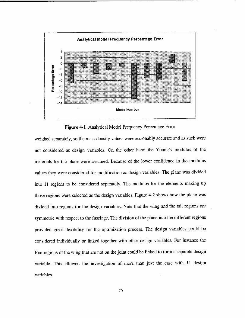
Analytical Model Frequency Percentage Error
t i— — - —
2 ^^^^^^^^^^^^^^^^^^^^^^^^^^M ^■;.;'-.
-9-
111 ro
r
i\i o
1:> qo' :sr ..-— ■ -r—j
6 » 10
iillj
Per
cent
age
Ei
i O
CO
CO
i
-
ISIllllllSllllllllllllBSS —
-12 j
Mode Number
Figure 4-1 Analytical Model Frequency Percentage Error
weighed separately, so the mass density values were reasonably accurate and as such were
not considered as design variables. On the other hand the Young's modulus of the
materials for the plane were assumed. Because of the lower confidence in the modulus
values they were considered for modification as design variables. The plane was divided
into 11 regions to be considered separately. The modulus for the elements making up
those regions were selected as the design variables. Figure 4-2 shows how the plane was
divided into regions for the design variables. Note that the wing and the tail regions are
symmetric with respect to the fuselage. The division of the plane into the different regions
provided great flexibility for the optimization process. The design variables could be
considered individually or linked together with other design variables. For instance the
four regions of the wing that are not on the joint could be linked to form a separate design
variable. This allowed the investigation of more than just the case with 11 design
variables.
70

_.
2 4 6
7
8
4 2
3 5 5 3
1
9 10 11 10 9
1. Body 2. Outer Forward Wing 3. Outer After Wing 4. Inner Forward Wing 5. Inner After Wing 6. Forward Wing Joint 7. Center Wing Joint 8. After Wing Joint 9. Outer Tail 10. Inner Tail
11. Tail Joint
Figure 4-2 Airplane Model Design Variable Regions
The sensitivity update method was used to update the finite element model
frequencies during the optimization iterations. The sensitivity values were computed by
the IDEAS software. The objective function for the optimization process was of the form
as shown in Equation (3-4), which is repeated below:
fx -fa ^ADVt OF = A*£lj „/' +B*S- 'k
i=l f," k=l DV„ (4.8)
where n is the number of modes and m is the number of design variables. The objective
function contains a frequency difference term and a change in design variables term. The
frequency term weighting multiplier, A, was set to ten while the change in design variable
term weighting multiplier, B, was set to zero. The constraints imposed on the solution
were that the individual frequency error terms were to be less than 5 percent and the
design variables were allowed to vary up to 40 percent.
71

There was another issue for the optimization process with the airplane model
which was not present for the computer simulation. The issue was which natural
frequencies to consider for the optimization process. The finite element model predicted
10 vibrational modes in the bandwidth for the test. However, not all of them were out-of-
plane modes. For example mode 9 was horizontal bending of the fuselage, with very little
deflection in the direction that the response accelerometers where set up to measure.
Modes 2 and 3 were also predominantly in-plane modes, but the wing and tail deflection
was significant enough to detect experimentally. Because of the difficulties in measuring
all of the modes, some optimization iterations were conducted with one or more of the
modes omitted.
4. Optimization Process
The optimization process was run numerous times to calculate candidate solution
sets. The sensitivities for the 11 regions of the airplane were combined to form as few as
five and as many as 11 design variables for an optimization run. The 2-level factorial
algorithm was used within the optimization run to investigate the different combinations
of the active design variables. The solution process was more volatile with multiple
design variables. The A multiplier needed to be adjusted frequently to ensure the solution
process would run to completion. There was a problem encountered within the
constrained optimization routine in MATLAB. If the multiplier for the frequency term
was not high enough, the routine would crash due to a magnitude error. While the routine
was attempting to go to the next iteration point, a fatal error would occur because one of
72

the numbers in the process would go to zero. Changing the A multiplier changes the slope
of the objective function preventing the deficiency in the routine from occurring.
Following the completion of the optimization runs a value for average frequency
error was calculated to be used as an initial evaluation method for each solution. Because
the finite element model was computed within IDEAS, the optimization process could not
automatically update the original finite element model. The candidate solutions were
entered by hand into IDEAS to calculate the new analytical frequencies and mode shapes
for comparison and final solution evaluation. The analytical mode shapes were reduced to
the same number of degrees of freedom of the experimental model by the extraction
method. This method was chosen because of the earlier simulations which showed no
advantage in solution accuracy for the other more complex methods.
5. Optimization Solution
The solution which was selected as optimal was computed with five design
variables and all ten frequencies. This solution had the lowest average error for all ten
frequencies and the highest MAC value of all of the runs. The specific frequency values
and errors are included in Appendix E in Table E-l. The design variable regions for this
solution and their designations in Figure 4-2 are:
• Fuselage (1)
• Wing - except for joint region (2,3,4, and 5)
• Wing joint region (6,7, and 8)
• Tail - except for joint region (9 and 10)
• Tail joint region (11)
73

The maximum change made to the any of the design variables was for the tail, and was a
31 percent increase from the original value. All of the design variable values were
increased with the exception of the fuselage. Figure 4-3 shows the effects of the updating
process on the frequency errors for the finite element model. The original model errors
are plotted with the updated model errors. The finite element model average frequency
error was reduced from 4.87 percent to 1.92 percent.
Frequency Percentage Error
o
LU O
a
6-t
4-i
2 -
0
-2 H
-4
-6
-8
-10
-12
-14
TT mm
''I III $ ORIGINAL
■ UPDATED
Mode Number
Figure 4-3 Frequency Error Comparison, Original and Updated Models
6. Solution Interpretation
The optimization process provided a solution set to update and improve the
performance of the finite element model. But what do the changes to the design variables
signify? The process indicates that the modulus in the wing, tail, and both joints should
be increased. The plate material and the joint characteristics are suffer than assumed for
the original model. This gives an indication why most of the natural frequencies were
74

originally predicted low by the model. These stiffness increases resulted in most of the
natural frequencies increasing in value. The wing and wing joint stiffness was increased
which raised the predicted frequencies for the wing modes; 1,5,7, and 10. The increases
in stiffness improved the accuracy for modes 1, 7 and 10 but overcompensated for mode
5 and actually increased the error magnitude. This demonstrates that it is difficult to
isolate particular modes with fairly large design variable regions. Smaller design variable
regions may have more success in correcting that model deficiency. The tail stiffness was
increased dramatically. This was to compensate for mode 6, which is tail bending, being
predicted rather low. The model prediction for this mode was probably quite low because
the mass density had been increased to compensate for a weld bead on the tail. The body
modulus was reduced to lower the frequencies that were fuselage dominated because
mode 9 was predicted high. In retrospect, the recommended changes to the material
properties tend to show where the mistakes were made in the construction of the finite
element model. This goes to demonstrate how hard some properties are to represent
accurately in the model. It also highlights the assumptions that were made for property
values or dimensions that incorrectly represented the true values.
D. COMPOSITE BEAM DAMAGE LOCALIZATION
1. Test Article and Finite Element Model Description
The experimental verification of the damage localization process was conducted
with two composite beams. One of the beams was undamaged while the other had a
known delamination 2.25 inches in length at its center. The beams were measured to
determine physical dimensions. These articles were the basis for the composite beam
75

models and the properties used in the Chapter HI computer simulations. The assumed
value for Young's modulus of the beam is the value identified in Reference (14). Specific
beam data is included in Appendix B.
Beam dynamic response was measured experimentally with a frequency
bandwidth of 1200 Hertz. The response of the each beam was measured at a single point,
which was located at the left end of the beam. The excitation force was applied in 25
different locations along the length of the beams. A diagram of the excitation point layout
for data collection is included in Appendix F as Figure F-l. A polynomial curve fit
procedure was used to generate the experimental mode shapes for the test pieces. The
experimental mode shapes for the damaged beam are included in Appendix F as Figures
F-2 through F-10.
2. Finite Element Model Update
The experimental data from the undamaged beam was used to update a finite
element model to develop the baseline model for the beam. The updated model could
then be used to detect and localize damage in a similar beam. The design variable for the
model updating procedure was Young's modulus of the composite beam. The first five
natural frequencies were utilized in the update procedure. The optimization process
increased the value of the modulus to match the experimental frequencies of the
undamaged beam. The results of the optimization process are included in Table 4-2.
76
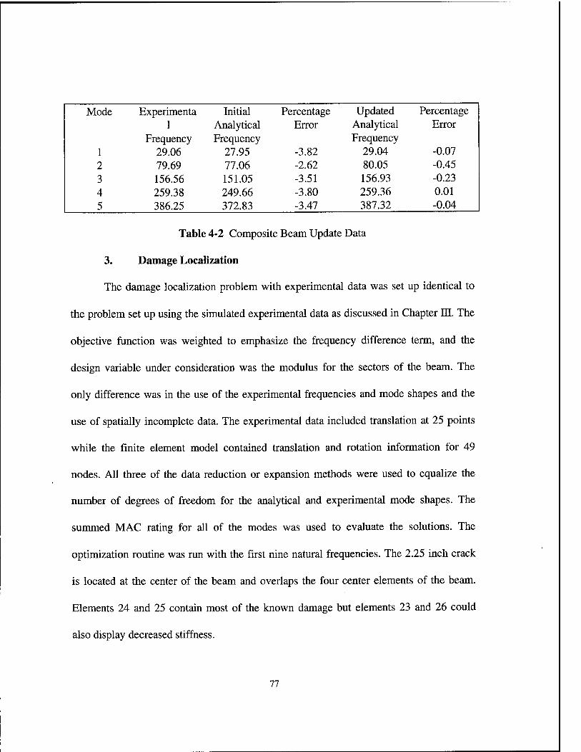
Mode Experimenta Initial Percentage Updated Percentage 1 Analytical Error Analytical Error
Frequency Frequency Frequency 1 29.06 27.95 -3.82 29.04 -0.07 2 79.69 77.06 -2.62 80.05 -0.45 3 156.56 151.05 -3.51 156.93 -0.23 4 259.38 249.66 -3.80 259.36 0.01 5 386.25 372.83 -3.47 387.32 -0.04
Table 4-2 Composite Beam Update Data
3. Damage Localization
The damage localization problem with experimental data was set up identical to
the problem set up using the simulated experimental data as discussed in Chapter HI. The
objective function was weighted to emphasize the frequency difference term, and the
design variable under consideration was the modulus for the sectors of the beam. The
only difference was in the use of the experimental frequencies and mode shapes and the
use of spatially incomplete data. The experimental data included translation at 25 points
while the finite element model contained translation and rotation information for 49
nodes. All three of the data reduction or expansion methods were used to equalize the
number of degrees of freedom for the analytical and experimental mode shapes. The
summed MAC rating for all of the modes was used to evaluate the solutions. The
optimization routine was run with the first nine natural frequencies. The 2.25 inch crack
is located at the center of the beam and overlaps the four center elements of the beam.
Elements 24 and 25 contain most of the known damage but elements 23 and 26 could
also display decreased stiffness.
77

4. Localization Results
The first trial investigated the localization process with spatially incomplete data.
The method used for mode shape equalization was analytical mode shape reduction using
the extraction method. The aset data from the analytical model mode shapes was
extracted and compared to the experimental mode shapes to compute the MAC. The
results of the search procedure are included in Table 4-3. The MAC values themselves are
not included in the table but the region with the highest rating is highlighted to indicate
the search results. Extraction provided the correct identification of the damage in the
center elements.
Damage in Elements 24-25
1st Iteration 1-16 17-32 33-48 1-48 Sectors
2nd Iteration 17-21 22-27 28-32 17-32 Sectors
3rd Iteration 22-23 24-25 26-27 22-27 Sectors
Table 4-3 Composite Beam Damage Search Results, Extraction Method
The next trial investigated the localization process with the reduction of the
analytical mode shapes using the Static Reduction transformation matrix. Results are
contained in Table 4-4.
78

Damage in Elements 24-25
1st Iteration 1-16 17-32 33-48 1-48 Sectors
2nd Iteration 17-21 22-27 28-32 17-32 Sectors
3rd Iteration 22-23 24-25 26-27 22-27 Sectors
Table 4-4 Composite Beam Damage Search Results, Static Reduction
The next trial investigated the localization process with expansion of the
experimental mode shapes using the Static Reduction transformation matrix. Results are
contained in Table 4-5.
Damage in Elements 24-25
1st Iteration 1-16 17-32 33-48 1-48 Sectors
2nd Iteration 17-21 22-27 28-32 17-32 Sectors
3rd Iteration 22-23 24-25 26-27 22-27 Sectors
Table 4-5 Composite Beam Damage Search Results, Static Expansion
The next trial investigated the localization process with the reduction of the
analytical mode shapes using the Improved Reduction System (IRS) transformation
matrix. Results are contained in Table 4-6.
79

Damage in Elements 24-25
1st Iteration 1-16 17-32 33-48 1-48 Sectors
2nd Iteration 17-21 22-27 28-32 17-32 Sectors
3rd Iteration 22-23 24-25 26-27 22-27 Sectors
Table 4-6 Composite Beam Damage Search Results, IRS Reduction
The next trial investigated the localization process with expansion of the
experimental data using the Improved Reduction System (IRS) transformation matrix.
Results are contained in Table 4-7.
Damage in Elements 24-25
1st Iteration 1-16 17-32 33-48 1-48 Sectors
2nd Iteration 17-21 22-27 28-32 17-32 Sectors
3rd Iteration 22-23 24-25 26-27 22-27 Sectors
Table 4-7 Composite Beam Damage Search Results, IRS Expansion
5. Solution Interpretation
All five of the solutions from the damage localization routines converge to the
two center elements as the most probable location of damage, which is the location of the
known damage. This successful demonstration of the localization process shows that the
sector search logic combined with the optimization routine can locate damage in a simple
80

test structure using spatially incomplete data. As far as the methods of compensating for
spatially incomplete data all of the techniques investigated were successful. Without a
performance advantage for any of the methods the one that requires the least
computational time should be used. The extraction method requires no computations
other than identifying and extracting the aset data points so that method should be
employed.
Four other composite beams with known damages were also tested to determine if
the damage could be localized. The experimental frequency data for the beams was not
consistent enough to allow the process to succeed. That is, the frequency shifts induced
by the reduction of stiffness in the beam did not provide a consistent downward trend for
all natural frequencies as compared to the undamaged beam. Without consistent
frequency shifts the optimization and damage localization process will not be successful.
Therefore the extent of the damage will remain unknown.
E. STEEL BEAM DAMAGE LOCALIZATION
1. Test Article and Finite Element Model Description
The experimental verification of the damage localization process was also
investigated with a steel beam test piece. The beam was tested in the undamaged state to
update the finite element model and then notched to simulate stiffness reduction. The
beam was measured directly to determine physical dimensions. The assumed value for
Young's modulus of the beam was the standard value used for steel. Specific beam data is
included in Appendix G.
81

Beam dynamic response was measured experimentally with a frequency
bandwidth of 2500 Hertz. The response of the beam was measured at a single point,
which was located at the left end of the beam. The excitation force was applied in 25
different locations along the length of the beam. A diagram of the excitation point layout
for data collection is included in Appendix G as Figure G-2. A polynomial curve fit
procedure was used to generate the experimental mode shapes for the test pieces. The
experimental mode shapes for the damaged beam are included in Appendix G as Figures
G-3 through G-12.
2. Finite Element Model Update
The experimental data from the beam in the undamaged condition was used to
update a finite element model to develop the baseline model for the beam. The updated
model could then be used to detect and localize damage in the test piece. The design
variable fro the model updating procedure was Young's modulus of the beam. The first
five natural frequencies were utilized in the update procedure. The optimization process
decreased the value of the modulus to match the experimental frequencies of the
undamaged beam. A MAC calculation was done to determine how well the analytical
mode shapes matched the experimental mode shapes. All five of the mode shapes had
MAC values greater than 0.99 indicating very good correlation of the analytical results to
the experimental mode shapes. The results of the optimization process are included in
Table 4-8.
82

Mode Experimenta Initial Percentage Updated Percentage 1 Analytical Error Analytical Error
Frequency Frequency Frequency 1 56.25 57.54 2.29 56.186 -0.11 2 155.00 158.62 2.33 154.89 -0.01 3 303.75 310.97 2.37 303.66 -0.01 4 501.25 514.08 2.56 502.0 0.01 5 746.875 768.00 2.83 749.96 0.01
Table 4-8 Steel Beam Update Data
3. Damage Localization
The damage localization problem for the steel beam was set up identical to the
problems explored for simulated tests in Chapter HI and for the experimental composite
beam test. The objective function was weighted to emphasize the frequency difference
term, and the design variable under consideration was the modulus for the sectors of the
search. The experimental data included relative translation at 25 points while the finite
element model contained translation and rotation information for 49 nodes. All three of
the data reduction or expansion methods were used equalize the number of degrees of
freedom for the analytical and experimental mode shapes. The summed MAC rating for
all of the modes was used to evaluate the solutions. The optimization routine was run
with the first nine natural frequencies. The damage condition was induced by notching the
beam. The reduction in cross sectional area was made in element 25 and resulted in a
decrease of 9.22 percent to the moment of inertia in that element, effectively reducing the
stiffness of the beam.
83

4. Solution Method
The initial trials for the steel beam optimization routine did not provide a solution
for the change to the design variable needed to update the model. The solution process
continually returned the initial value of the design variable as the optimal solution. This
was due to the errors in the analytical frequencies versus the experimental frequencies.
The analytical model predicted the low frequencies high and the high frequencies low.
The relative error was about equal so the routine determined that the system was at the
optimal solution. To compensate for the inability of the optimization process to solve for
the change to the design variable another method was used. This method is similar to the
direct solve method discussed in Chapter in and is called the pseudo-inverse method.
This method uses an overdetermined matrix equation to solve for the change to a single
design variable. The sensitivity matrix, [T], is reduced to a 9 x 1 vector. The vector is
transposed and the individual terms are inverted. This procedure is called the pseudo-
inverse of a non-square matrix. The solution for the single design variable change can
then be computed as follows:
ADV= [pinv(T)]{A f} (4.9)
where pinv indicates the pseudo-inverse procedure. This procedure does provide a
solution for the reduction in the design variable that is used for the sector search.
5. Localization Results
The use of the pseudo-inverse solution method did allow the routine to compute a
value for the change to the modulus within a region. The search procedure was not
84

successful though. The process tended to select the overall regions instead of one of the
three sectors for the search. The results for this damage case are shown in Table 4-9.
Damage in Element 25
1st Iteration 1-16 17-32 33-48 1-48 Sectors
2nd Iteration 17-21 22-27 28-32 17-32 Sectors
Table 4-9 Steel Beam Damage Search Results, Extraction Reduction
The process indicates the overall region for the second iteration. In fact the next
highest MAC value was for the right sector, elements 28 to 32, so even if the overall
region selection was ignored the known solution would not be selected. None of the
methods of compensating for the spatially incomplete data made the results improve in
accuracy.
6. Simulated Experimental Damage
To investigate why the process did not work for this test piece, the experimental
damage condition was simulated by making adjustments to the baseline finite element
model. The simulated experimental data set was then compared to the experimental data.
The comparison data is contained in Table 4.10. The simulated experimental data was
reduced to be spatially incomplete by the extraction method, that is the aset points were
extracted from the simulated modal data.
85

Mode Experimental Simulated Percentage MAC Frequency Frequency Error
1 56.25 56.02 -0.41 0.9987 2 154.688 154.89 0.13 0.9974 3 303.125 302.99 -0.04 0.9972 4 501.562 501.97 0.09 0.9973 5 746.88 748.33 0.19 0.9924 6 1042.19 1047.37 0.50 0.9921 7 1381.25 1391.88 0.77 0.9823 8 1768.75 1791.16 1.27 0.9907 9 2201.56 2233.85 1.47 0.9917
Table 4-10 Simulated Experimental Data Comparison
The major differences are observed in the simulated frequencies as compared to
the experimental frequencies. The MAC values rate how well the individual simulated
modes correlate to the experimental modes. Ratings in excess of 0.99 indicate very good
correlation. The solution process was then run with the simulated experimental data. The
simulated experimental mode shapes were spatially complete. The aset data was extracted
to generate spatially incomplete experimental mode shapes. The results for that case are
included in Table 4-11.
Damage in Element 25
1st Iteration 1-16 17-32 33-48 1-48 Sectors
2nd Iteration 17-21 22-27 28-32 17-32 Sectors
3rd Iteration 22-23 24-25 26-27 22-27 Sectors
4th Iteration 23 24 25 23-25 Sectors
Table 4-11 Steel Beam Damage Search Results, Simulated Experimental Data
86

The process successfully identified the damage for the simulated experimental
case. At this point the natural frequencies and mode shapes of the actual experimental
data set were substituted for the simulated experimental data to determine which factors
caused the actual experiment to fail in damage localization. Table 4-12 summarizes the
results of inserting the experimental data into the simulated experimental data set.
Modes Frequency Shapes Both 1 25 25 25 2 25 25 25 3 25 25 25 4 25 17-32/24-25 17-32/24-25 5 25 31 31 6 25 30 30 7 17-32/24-25 30 17-32/24-25 8 17-32/24-25 22-27 17-32/24-25 9 17-32/26-27 25 17-32/22-27
1-3 25 25 25 4-6 25 30 30 7-9 17-32/22-27 30 17-32/22-27 1-9 17-32/22-27 30 17-32/28-32
Table 4-12 Experimental Data Substitution Results
a. Frequency Substitution
The experimental frequencies were substituted into the simulated
experimental data set both one at a time and in groups. Changing the frequencies for the
first six modes of the simulated data set individually, had no effect on the solution. The
process converged to element 25 as had been previously observed for the simulated data.
When the frequencies for mode seven or mode eight were substituted into the data set, the
process selected elements 17 to 32 instead of the center sector. This result was ignored to
determine if the problem existed in the rating of the overall region. Selecting the highest
87

sector, which was the center, iterations were continued to see if a single element could be
identified. The next iteration selected elements 24 and 25 but a final iteration did not
select element 25.
The natural frequencies were then substituted in groups. The first group
consisted of the frequencies for first three modes. This did not change the results.
Substituting the frequencies for modes 4 to 6 did not change the results either.
Substituting the frequencies for modes 7 to 9 again caused the process to select elements
17 to 32. This response was ignored and another iteration was run which selected sector
22 to 27. Substituting the frequencies for all nine modes had the same effect as
substituting the frequencies for modes 7 to 9.
This substitution process indicates that the frequencies for the high modes
contaminate the solution process in some fashion to create error. The probable problem is
that the large frequency difference between the analytical and experimental results force
the pseudo-inverse solution to be too large. This creates error when the updated mode
shapes are calculated and results in the MAC selecting the larger region.
b. Mode Shape Substitution
The experimental mode shapes were then substituted into the simulated
experimental data set one at a time and in groups. Substituting the first three mode shapes
individually had no effect. Substituting the fourth mode shape caused the process to select
elements 17 to 32. If that selection was ignored the next iteration selected elements 24
and 25. Substituting the fifth mode shape resulted in the selection of element 31 as the
damage location. Substituting both the sixth and seventh mode shapes resulted in the

selection of element 30 as the damage location. The eight mode shape resulted in the
selection of elements 22 to 27 and the ninth mode shape had no effect.
The mode shapes were then substituted in groups. Mode shapes 1 to 3 had
no effect on the solution. Substituting mode shapes 4 to 6 caused the process to select
element 30. Substituting mode shapes 7 to 9 and 1 to 9 both lead to the process selecting
element 30.
The substitution of the mode shapes indicates that the mode shapes are not
the same as those predicted by the simulated damage finite element model. Even though
the MAC between the simulated damage mode shapes and experimental modes shapes
indicates a good match it is not good enough. Also the higher modes are less similar to
the experimental data. The higher mode shapes contaminate the solution so the process
selects the wrong elements. This could be caused by noise, faulty data taking, or an error
in the process used to calculate the mode shapes.
c. Frequency and Mode Shape Substitution
The experimental frequencies and mode shapes were then substituted into
the simulated experimental data set one mode at a time and in groups. Substituting the
first three modes individually had no effect. Substituting the fourth mode caused the
process to select elements 17 to 32. If that selection was ignored the next iteration
selected elements 24 and 25. Substituting the fifth mode resulted in the selection of
element 31 as the damage location. Substituting the sixth mode resulted in the selection
of element 30 as the damage location. Substituting the seventh mode or the eight mode
resulted in the selection of elements 17 to 32. This was ignored and another iteration
89

selected elements 24 and 25. Substituting the ninth mode resulted in selecting elements
22-27.
The modes were then substituted in groups. Modes 1 to 3 had no effect on
the solution. Substituting modes 4 to 6 caused the process to select element 30.
Substituting mode shapes 7 to 9 caused the process to select elements 17 to 32. Another
iteration selected elements 22 to 27. Substituting modes 1 through 9 lead to the process
selecting elements 28 to 32.
The substitution of both the frequencies and the mode shapes indicates that
the data from the experimental data set is not "clean" enough to select the known damage
location. The problem with the data could be any one of the items cited for the mode
shape problems. The results for the lower modes would seem to indicate that if a solution
was run just considering the lower modes that the correct damage location would be
identified, but that was not the case.
7. Solution Interpretation
The unsuccessful trials for the steel beam indicate that the sector search method
does have some limitations. The experimental data set needs to be extremely clean or the
search process will be ineffective. Even the smallest noise or other contamination will
cause errors in the process. Another problem is the inability of the optimization routine to
run for the steel beam. The frequency differences should cause the routine to search for an
optimum value but it does not. This may be due to a problem in the sensitivity matrix, but
that does not account for the process working for beam optimization or the pseudo-
90

inverse solve procedure. This test case does indicate that further study in necessary on the
sector search form damage localization.
91

92

V. CONCLUSIONS / RECOMMENDATIONS
A. SUMMARY
Sensitivity-based finite element model updating and numerical optimization
procedures were developed to improve finite element model performance and to detect
structural damage. Experimentally measured dynamic responses were compared to
analytically predicted dynamic responses to provide a basis to make corrections to design
parameters of the finite element model. The investigation of updating procedures and
applications have shown the following:
• The updating and optimization procedures provide a means to modify finite
element models to improve their accuracy, or to determine structural damage
by a comparison of experimentally measured dynamic responses to those
predicted by the finite element model.
• Sensitivity based updating of analytical natural frequencies for small changes
to design parameters is a valid method of approximation that reduces
computational requirements during the optimization process.
• Numerical optimization methods provide a logical search procedure and
enhance computational efficiency in the determination of the corrections that
need to be made in order to update finite element models.
• The 2-level factorial search algorithm provides a thorough means to test
different combinations of design variables to ensure the best solution is
attained. However, the number of iterations for this method increases
93

exponentially with the number of design variables, precluding its use for
problems with large numbers of design variables.
• The sector search methodology provides a logical search procedure to isolate
damage to a specific region of structure.
• The Modal Assurance Criterion provides a means to select the optimal
solution during the optimization process by evaluating which candidate
solution mode shapes most closely match the experimental data.
• The effectiveness of these procedures is directly dependent on the quality of
the experimental measurements.
B. CONCLUSIONS
The processes investigated for model updating were effective in determining
changes to be made to a finite element model to more closely resemble the response of
the structure being modeled. These processes not only improve the performance of the
finite element model but enhance the analyst's understanding of the finite element model
and the structure itself. The process of identifying the design parameters and examining
the specifics of the system dynamic responses, increases the level of understanding of
how individual sections and their physical properties affect the overall characteristics of
the system. The two applications highlight different points about the process.
The model update problem is dependent on the number and type of design
parameters chosen for evaluation. The parameters should be chosen with care to ensure
that they allow the isolation of specific mode shapes and frequencies while at the same
time not overloading the computational capabilities in the process. The modifications to
94

model parameters determined by the process tended to highlight faulty assumptions or
property values which could not be represented with high confidence. The solutions are
also dependent on the bandwidth of experimental data available for comparison.
The composite beam damage localization process demonstrated that the sector
search logic and model updating could be used to locate damage. This process is highly
dependent on the structure having a previously validated finite element model to provide
baseline response data. This process is also dependent on the damage condition inducing
a consistent pattern of frequency errors from the baseline model.
The damage localization problem with the steel beam highlights some of the
problems in comparing the analytical responses to the experimental response. The
frequencies predicted by the finite element model for the undamaged beam diverged from
the actual results. The higher system frequencies of the baseline model had relatively high
error levels and contaminated the solution process preventing damage localization. The
accuracy of the mode shape measurements also played a role in this test not being
successful. Without highly accurate experimental mode shapes the process will identify
the wrong location for damage.
C. RECOMMENDATIONS
The model updating procedures and routines developed showed positive results
both for simulated and actual experimental data. However, there were limitations in the
ability to pass data from one software type to another for the model update procedure, and
the damage localization procedure did not work on both test pieces. Recommendations to
address these and other shortcomings of these processes include:
95

• Continue to develop routines to pass data directly between the software used
for optimization, MATLAB, and the software used for finite element model
simulation, such as IDEAS.
• Modify the optimization processes to utilize mode shape sensitivities for use
with MAC solution evaluation vice re-solving the eigenproblem.
• Modify the optimization routine to allow more flexibility in its application, by
allowing for direct user interface with the use of pull down menus or prompts
removing the need to hardcode for a given model type.
• Continue to investigate the process of model updating by applying the baseline
software to more complex structures.
• Develop more efficient methods of combining design variables to allow
isolation of all modeling errors while not requiring excessive iterations.
• Continue to research the sector search method of damage localization to both
isolate why the method failed for the steel beam, and to apply the logic to
larger and more complex structures.
• Employ aset and oset information to effectively increase the bandwidth of
experimental testing.
• Employ more advanced means of measurement to remove possible errors due
to noise or other signal contamination.
The ability to pass mode shape or design variable data directly from IDEAS to
MATLAB or vice versa would greatly enhance the efficiency of the updating process.
The time required to format data to put into MATLAB or to feedback design variable
96

modifications into simulation software greatly limits the size and number of solutions that
can be investigated during optimization. Direct conversion will be required for larger
models.
Mode shape sensitivities can be used to approximate the change to the mode
shapes of a system based on the change to design parameters. By using this
approximation the need to re-solve the eigenproblem to evaluate every candidate solution
is removed and would greatly increase computational efficiency.
The computer codes used in this thesis were hardcoded to the specific situation.
Although all of the processes would be similar, the ability to apply this method to other
situations requires user modification of the code. Methods to improve user interface
should be developed.
The processes developed could be expanded to handle larger and more complex
systems. The updating logic could be applied to finite element models generated by other
students for specific pieces of equipment. This would improve both the models being
analyzed and the optimization code. The sector search logic could be expanded to include
a way to deal with shell elements or for complex geometry than the beam elements tested.
The 2-level factorial algorithm employs large numbers of iterations to investigate
all possible design variable combinations. Other methods of examining design variable
combinations that allow isolation of errors while not requiring excessive computer time
should be developed. This would greatly improve the computational efficiency of the
optimization process.
97

The ability to extract more data from a test bandwidth could be explored through
the use of aset and oset system frequencies. Basically the methods allow the analyst to
process test data as if measurement points were fixed, effectively introducing a new set of
boundary conditions. This would increase the number of system frequencies that could be
used in the sensitivity equations.
The ability of a process to accurately update a model or to localize damage are
dependent on the quality of the measured test data. Without accurate natural frequencies
and mode shapes the process can not be expected to succeed for either application.
98

APPENDIX A. ALUMINUM BEAM SPECIFICATIONS
A. PHYSICAL DIMENSIONS AND PROPERTIES
The aluminum beam used for the Chapter in computer simulations was not
patterned after a actual test piece. The dimensions of the beam were chosen at random
and the physical properties were chosen from standard material data for aluminum. The
beam orientation for the simulations was as depicted in Figure A-l. The degrees of
freedom were the vertical translation, upward in the figure, and rotation around a vector
out of the plane of the page.
D
W
L = 10 feet D = 10 inches W = 3 inches
Figure A-l Aluminum Beam
The physical properties chosen for the beam were:
Young's modulus E = 10 e 6 PSI mass density p = 0.000254 lbf-sec2/in4
B. DYNAMIC RESPONSE
The system natural frequencies predicted by the finite element model are:
Mode 1 22.26 Hz Mode 2 139.50 Hz Mode 3 390.82 Hz Mode 4 767.11 Hz
The mode shapes predicted by the finite element are included in Figures A-2 through A-5.
99

0 Mode Shi ape 1
™ . I I I 1
-0.1 ^-\ -
-0.2 -
Def
lect
ion
6 - -
CD
"I -0.4 CD
CC
-
-0.5 \
-0.6
i i i i ' > ' 5
Node
Figure A-2 Aluminum Beam, 1st Mode Shape
Mode Shape 2 0.8
Figure A-3 Aluminum Beam, 2nd Mode Shape
100

Mode Shape 3
Figure A-4 Aluminum Beam, 3rd Mode Shape
Mode Shape 4 0.6
Figure A-5 Aluminum Beam, 4th Mode Shape
101
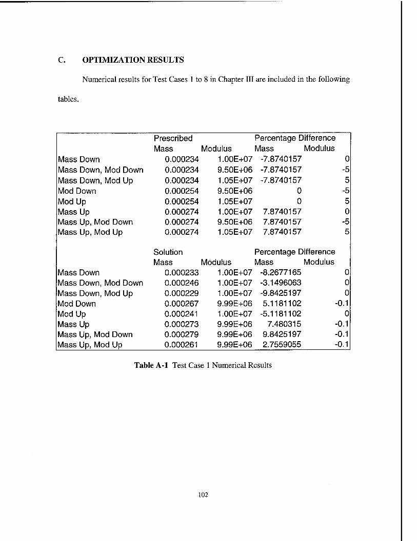
OPTIMIZATION RESULTS
Numerical results for Test Cases 1 to 8 in Chapter III are included in the following
tables.
Prescribed Percentage Difference Mass 1 Modulus Mass Modulus
Mass Down 0.000234 1.00E+07 -7.8740157 0 Mass Down, Mod Down 0.000234 9.50E+06 -7.8740157 -5 Mass Down, Mod Up 0.000234 1.05E+07 -7.8740157 5 Mod Down 0.000254 9.50E+06 0 -5 Mod Up 0.000254 1.05E+07 0 5 Mass Up 0.000274 1.00E+07 7.8740157 0 Mass Up, Mod Down 0.000274 9.50E+06 7.8740157 -5 Mass Up, Mod Up 0.000274
Solution
1.05E+07 7.8740157
Percentage Difference
5
Mass 1 Modulus Mass Modulus Mass Down 0.000233 1.00E+07 -8.2677165 0 Mass Down, Mod Down 0.000246 1.00E+07 -3.1496063 0 Mass Down, Mod Up 0.000229 1 .OOE+07 -9.8425197 0 Mod Down 0.000267 9.99E+06 5.1181102 ■0.1 Mod Up 0.000241 1 .OOE+07 -5.1181102 0 Mass Up 0.000273 9.99E+06 7.480315 ■0.1 Mass Up, Mod Down 0.000279 9.99E+06 9.8425197 ■0.1 Mass Up, Mod Up 0.000261 9.99E+06 2.7559055 -0.1
Table A-l Test Case 1 Numerical Results
102

Prescribed Percentage Difference Mass Modulus Mass Modulus
Mass Down 0.000234 1 .OOE+07 -7.8740157 0 Mass Down, Mod Down 0.000234 9.50E+06 -7.8740157 -5 Mass Down, Mod Up 0.000234 1.05E+07 -7.8740157 5 Mod Down 0.000254 9.50E+06 0 -5 Mod Up 0.000254 1.05E+07 0 5 Mass Up 0.000274 1 .OOE+07 7.8740157 0 Mass Up, Mod Down 0.000274 9.50E+06 7.8740157 -5 Mass Up, Mod Up 0.000274
Solution
1.05E+07 7.8740157
Percentage Difference
5
Mass I y/lodulus \/lass Modulus Mass Down 0.000237 1.02E+07 -6.6929134 1.9 Mass Down, Mod Down 0.000252 1.02E+07 -0.7874016 2.4 Mass Down, Mod Up 0.000229 1.04E+07 -9.8425197 3.97 Mod Down 0.000267 9.99E+06 5.1181102 -0.1 Mod Up 0.0002413 9.99E+06 -5 -0.1 Mass Up 0.0002725 9.99E+06 7.2834646 -0.1 Mass Up, Mod Down 0.000273 9.54E+06 7.480315 -4.6 Mass Up, Mod Up 0.000261 9.99E+06 2.7559055 -0.1
Table A-2 Test Case 2 Numerical Results
103

Prescribed Percentage Difference Mass f Modulus Mass Modulus
Mass Down 0.000234 1.00E+07 -7.8740157 0 Mass Down, Mod Down 0.000234 9.50E+06 -7.8740157 -5 Mass Down, Mod Up 0.000234 1.05E+07 -7.8740157 5 Mod Down 0.000254 9.50E+06 0 -5
Mod Up 0.000254 1.05E+07 0 5
Mass Up 0.000274 1.00E+07 7.87401575 0 Mass Up, Mod Down 0.000274 9.50E+06 7.87401575 -5 Mass Up, Mod Up 0.000274
Solution
1.05E+07 7.87401575
Percentage Difference
5
Mass 1 Modulus Mass Modulus Mass Down 0.00025 1.07E+07 -1.5748031 7 Mass Down, Mod Down 0.000252 1.02E+07 -0.7874016 2.4 Mass Down, Mod Up 0.000241 1.09E+07 -5.1181102 8.7 Mod Down 0.000255 9.52E+06 0.19685039 -4.8 Mod Up 0.000248 1.02E+07 -2.519685 2.49 Mass Up 0.000271 9.92E+06 6.53543307 -0.8 Mass Up, Mod Down 0.000263 9.15E+06 3.38582677 -8.55 Mass Up, Mod Up 0.000254 9.73E+06 0 -2.7
Table A-3 Test Case 3 Numerical Results
104

Prescribed 3ercentage Difference Mass f Modulus Mass Modulus
Mass Down 0.000234 1.00E+07 -7.874016 0 Mass Down, Mod Down 0.000234 9.50E+06 -7.874016 -5 Mass Down, Mod Up 0.000234 1.05E+07 -7.874016 5 Mod Down 0.000254 9.50E+06 0 -5 Mod Up 0.000254 1.05E+07 0 5 Mass Up 0.000274 1.00E+07 7.8740157 0 Mass Up, Mod Down 0.000274 9.50E+06 7.8740157 -5 Mass Up, Mod Up 0.000274
Solution
1.05E+07 7.8740157
Percentage Difference
5
Mass I Modulus Mass Modulus Mass Down 0.000255 1.09E+07 0.3937008 9.3 Mass Down, Mod Down 0.0002369 9.64E+06 -6.732283 -3.6 Mass Down, Mod Up 0.0002439 1.10E+07 -3.976378 10 Mod Down 0.000247 9.24E+06 -2.755906 -7.6 Mod Up 0.00026 1.08E+07 2.3622047 7.5 Mass Up 0.000261 9.56E+06 2.7559055 -4.4 Mass Up, Mod Down 0.0002715 9.50E+06 6.8897638 -5.02 Mass Up, Mod Up 0.000279 1.07E+07 9.8425197 7.3
Table A-4 Test Case 4 Numerical Results
105

Prescribed Value Percentage Difference Mass Modulus Mass Modulus
Mass Down 0.000234 1.00E+07 -7.874 0 Mass Down, Mod 0.000234 9.50E+06 -7.874 -5
Down Mass Down, Mod Up 0.000234 1.05E+07 -7.874 5
Mod Down 0.000254 9.50E+06 0 -5 Mod Up 0.000254 1.05E+07 0 5 Mass Up 0.000274 1.00E+07 7.874 0
Mass Up, Mod Down 0.000274 9.50E+06 7.874 -5 Mass Up, Mod Up 0.000274 1.05E+07 7.874 5
Solution Value Percentage Difference Mass Modulus Mass Modulu DV Combo Single
Mass Down 0.000233 1.00E+07 -8.307 0 M only 0.814 Mass Down, Mod 0.000246 1.00E+07 -3.15 0 Konly 0.837
Down Mass Down, Mod Up 0.000244 1.10E+07 -4.094 9.9 Both 0.833
Mod Down 0.000259 9.70E+06 1.969 -3.02 Both 0.824 Mod Up 0.000254 1.05E+07 0 5 Konly 0.8165 Mass Up 0.000273 1 .OOE+07 7.323 0 M only 0.814
Mass Up, Mod Down 0.000271 9.49E+06 6.693 -5.13 Both 0.812 Mass Up, Mod Up 0.000261 9.99E+06 2.559 -0.1 Both 0.796
Table A-5 Test Case 5 Numerical Results
106

Prescribed f Dercentage Difference Mass Modulus Mass Modulus
Mass Down 0.00024 1.00E+07 -5.5118 0 Mass Down, Mod 0.00024 9.20E+06 -5.5118 -8 Down Mass Down, Mod 0.00024 1.08E+07 -5.5118 8 Up Mod Down 0.000254 9.20E+06 0 -8 Mod Up 0.000254 1.08E+07 0 8 Mass Up 0.000268 1.00E+07 5.5118 0 Mass Up, Mod 0.000268 9.20E+06 5.5118 -8 Down Mass Up, Mod Up 0.000268 1.08E+07 5.5118 8
Solution Percentage Difference Mass Modulus Mass Modulus 3V Combo Single
Mass Down 0.000239 1.00E+07 -5.9055 0 M only 0.8151 Mass Down, Mod 0.000261 9.99E+06 2.7559 -0.1 Both 0.8509 Down Mass Down, Mod 0.000243 1.10E+07 -4.3701 9.9 Both 0.8215 Up Mod Down 0.000254 9.20E+06 0 -8 Konly 0.8156 Mod Up 0.000254 1.08E+07 0 8 Konly 0.8165 Mass Up 0.000267 1.00E+07 5.1181 0 M only 0.8153 Mass Up, Mod 0.000261 9.00E+06 2.7559 -10 Both 0.8059 Down Mass Up, Mod Up 0.000252 1.02E+07 -0.7087 1.67 Both 0.7921
Table A-6 Test Case 6 Numerical Results
107

Prescribed Value Percentage Difference Mass Modulus Mass Modulus
Mass Down 0.00024 1.00E+07 -5.5118 0 Mass Down, Mod 0.00024 9.20E+06 -5.5118 -8
Down Mass Down, Mod 0.00024 1.08E+07 -5.5118 8
Up Mod Down 0.00025 9.20E+06 0 -8
Mod Up 0.00025 1.08E+07 0 8 Mass Up 0.00027 1.00E+07 5.5118 0
Mass Up, Mod 0.00027 9.20E+06 5.5118 -8 Down
Mass Up, Mod Up 0.00027 1.08E+07 5.5118 8
Solution Value Percentage Difference Mass Modulus Mass Modulus DV Single
Combo Mass Down 0.00024 1.00E+07 -5.9055 0 M only 0.815
Mass Down, Mod 0.00025 9.62E+06 -1.2205 -3.82 Both 0.835 Down
Mass Down, Mod 0.00024 1.10E+07 -4.3307 9.9 Both 0.821 Up
Mod Down 0.00025 9.20E+06 0 -8 Konly 0.816 Mod Up 0.00025 1.08E+07 0 8 Konly 0.816 Mass Up 0.00027 1.00E+07 5.1181 0 M only 0.815
Mass Up, Mod 0.00028 9.72E+06 10 -2.81 Both 0.833 Down
Mass Up, Mod Up 0.00025 1.01E+07 -1.5748 0.9 Both 0.789
Table A-7 Test Case 7 Numerical Results
108

Prescribed Value Percentage Difference Mass Modulus Mass Modulus
Mass Down 0.00024 1.00E+07 -5.51 0 Mass Down, Mod 0.00024 9.20E+06 -5.51 -8
Down Mass Down, Mod 0.00024 1.08E+07 -5.51 8
Up Mod Down 0.000254 9.20E+06 0 -8
Mod Up 0.000254 1.08E+07 0 8 Mass Up 0.000268 1.00E+07 5.512 0
Mass Up, Mod 0.000268 9.20E+06 5.512 -8 Down
Mass Up, Mod Up 0.000268 1.08E+07 5.512 8
Solution Value Percentage Difference Mass Modulus Mass Modulus DV
Combo MAC
Mass Down 0.00024 1.00E+07 -5.71 0 M1 only 4 Mass Down, Mod 0.00024 9.20E+06 -5.35 -8.05 M1 + K1 4
Down Mass Down, Mod 0.00024 1.08E+07 -5.51 7.99 M1 + K1 4
Up Mod Down 0.000254 9.19E+06 0 -8.11 K1 only 4
Mod Up 0.000254 1.08E+07 0 7.9 K1 only 4 Mass Up 0.000268 1.00E+07 5.354 0 M1 only 4
Mass Up, Mod 0.000268 9.20E+06 5.551 -8.01 M1 + K1 4 Down
Mass Up, Mod Up 0.000268 1.08E+07 5.63 7.95 M1 + K1 4
Table A-8 Test Case 8 Numerical Results
109

110

APPENDIX B. COMPOSITE BEAM SPECIFICATIONS
A. PHYSICAL DIMENSIONS AND PROPERTIES
The composite beam used for the Chapter HI computer simulations was patterned
after sample test pieces. The beams are made of a continuous carbon fiber/epoxy. The
dimensions and the mass of the beam were measured. The original Young's modulus
value was the value calculated in Reference (14). The beam orientation for the
simulations was as depicted in Figure B-l. The degrees of freedom for the beam were
vertical translation, upward in the figure, and rotation around a vector out of the plane of
the page.
D: 7 w
L = 4 feet D = 0.2911 inches W = 5.723 inches
Figure B-l Composite Beam
The original physical properties assumed for the beam were:
Young's modulus E = 6.33e6 PSI mass density p = 0.0001328 lbf-sec2/in4
Young's modulus was updated using the optimization procedure and comparison to the
undamaged beam's dynamic response. The updated value was:
Young's modulus E = 6.76 e 6 PSI
111

B. DYNAMIC RESPONSE
The system natural frequencies predicted by the finite element model are:
Mode 1 28.96 Hz Mode 2 79.85 Hz Mode 3 156.6 Hz Mode 4 258.9 Hz Mode 5 386.9 Hz Mode 6 540.5 Hz Mode 7 719.8 Hz Mode 8 924.8 Hz Mode 9 1155.6 Hz
The mode shapes predicted by the finite element are included in Figures B-2 through B-
10.
Mode Shape 1
10 15 20 25 30 Node
35 40 45 50
Figure B-2 Composite Beam Analytical Mode Shape 1
112

Mode Shape 2 0.3
Figure B-3 Composite Beam Analytical Mode Shape 2
-0.25 i i_
35 40 45 50
Figure B-4 Composite Beam Analytical Mode Shape 3
113

0.25 Mode Shape 4
20 25 30 Node
Figure B-5 Composite Beam Analytical Mode Shape 4
Mode Shape 5 0.2
20 25 Node
Figure B-6 Composite Beam Analytical Mode Shape 5
114

0.25
0.2
Mode Shape 6
0.15 "I A A A " 0.1
c
J 0.05 CD O CD
■M o CO
CD EC
-0.05 : A A A;
-0.1 - \ / \ / \ / I - -0.15
' ( } 5 10 15 20 25 30 35 40 45 50 Node
Figure B-7 Composite Beam Analytical Mode Shape 6
Mode Shape 7
0.15
0.1 / \ / \ / \ \ '
Rel
ativ
e D
efle
ctio
n i
6
o
9
ö
b
-0.15 - j \ J \ J \ 1
-0.2
( ) 5 10 15 20 25 30 35 40 45 5 Node
Figure B-8 Composite Beam Analytical Mode Shape 7
0
115

Mode Shape 8
Figure B-9 Composite Beam Analytical Mode Shape 8
0.2 r Mode Shape 9
-| 1 1 1 1 T"
0.1
_o o a>
"Hi a Oh CD .>
tr
-0.1
-0.2i:
Figure B-10 Composite Beam Analytical Mode Shape 9
116

APPENDIX C. EXPERIMENTAL SETUP
The experimental setup involved the selection of test equipment and of test
settings. The following equipment and software was used for measurement of the test
pieces dynamic responses and signal processing or analysis:
• PCB load cell
• PCB accelerometers
• PCB Model 483A Amplifier
• Zonic Workstation 7000 Signal Analyzer
• HP Series 700 computer
• IDEAS Master Series 2.1 Software
Figure C-l depicts the experimental setup. Calibration data for the measurement
equipment is included on the following pages.
Test Piece
Acceleromete
Impact Hammer with Load Cell
Ch.2
Amplifier
Ch.1
Ethernet
Cable
HP 700 Computer
Zonic Workstation
Figure C-l Experimental Setup
117

PCB CALIBRATION CERTIFICATE pro PIEZOTRONICS
IMPULSE FORCE HAMMER
Model Nc. 0B6B03
Serial No. _ 2194
Range 0~500 |b
Linearity error <l.f
Discharge Time Constant 2000 s
Output Impedance _
Output Bias 9 • 1
.ohms
. volts
737/236305
Customer: N/A^L- PöS I &QflQl»Ufc
SCHOOL-
Invoice No.:
3S77L
Calibration Specification Ml L-STD 45662
f~ <??-&(* Traceable toJJBS through
Initials f'fl Date:
Accelerometer: Model No. 302R07 Serial No Z£!Z_ Sens. 9-91 mV/g
Pendulous Test Mass * • 05 11> ( iZJLgram) including accelerometer
Hammer Sensitivity:
CONFIGURATION Tip PLRSTIC/VINYL PLRSTIC/VINYL
Extender NONE STEEL
SCALING FACTOR Ib/g 1.03 0.98 (SENSITIVITY RATIO)
(SEE NOTE)
Accel/Force (N/ms-2) 0.47 0.44
mV/lb 9.59 10. 1
HAMMER - SENSITIVITY
(mV/N) 2.15 2.26
NOTES:
1. The sensitivity ratio (Sa/Sf) is the scaling factor for converting structural transfer measurements into engineering units. Divide results by this ratio.
2. Each specific hammer configuration has a different sensitivity. The difference is a constant percentage, which depends on the mass of the cap and tip assembly relative to the total mass of the head. Calibrating the specific hammer structure being used automatically compensates for mass effects.
Effective mass 0.265 with 302A07 attached and vinyl capped plastic tip.
PCB PIEZOTRONICS, INC. 3425 WALD6N AVENUE OEPEW. NEW YORK 14043-2495 TELEPHONE 716-684-0001 TWX 710-263-1371
118

@=s=a (C PerlSA-RP37.2
Model No. ■tffittM
Serial No. 117R7
PO No. Cust
Calibration traceable to NIST thru Project No. B22/2511B1-33
CALIBRATION DATA
Voltage Sensitivity 96.3 mV/g
Transverse Sensitivity £5.0 %
Resonant Frequency >_ 7 kHz
Time Constant (NOM.) B.5 s
Output Bias Level 9.1 V
e@5©
ICP* ACCELEROMETER with buill-in electronics
Calibration procedure is in compliance with MIL-STD-45662A and traceable to NIST.
KEY SPECIFICATIONS
Range 50 ±g
Resolution 0.001 g
Temp. Range 0/+150 °F
METRIC CONVERSIONS:
ms? = 0.102 g
°C = 5/9 x (»F -32)
Reference Freq
Frequency Hz 10 15 30 50 100 300 500 1000 2000
Amplitude Deviation % 3.4 2.4 1.8 .8 0.0 -.9 -.9 -.e 2.5
h3dB
Amplitude
Deviation
-3 dB
PCB
FREQUENCY RESPONSE
0 1 a D F requen cy in Hen z c 0 0 10 000
Piezotronics, Inc. 3425 Waiden Avenue Depew, NY 14043-2495 USA 716-684-0001 Calibrated by
Date 2/17/94
CODE: CC-ENG
119

Calibration ^LJata ACCELEROMETER MODEL 225BR-10 SERIAL NO. BNB 1
Sensitivity 18.10 mV/q(a> ma Hz, m g's pK
MAXIMUM TRANSVERSE SENSITIVITY:
DEV X FREQUENCY RESPONSE
1 1 1
20
IR
5
BX
i
j
-5
10
i i ,
i 10 100 1K
FREQUENCY IN Hz
DEV dB
40
20
0dB
-20
10K 50K
J01 ;
^ A. ENDEVCO Date.
By. All calibrations are traceable to the National Bureau o( Standards and in accordance with MIL-STD-45662 This certifies that this accelerometer meets all tue performance, environmental and physical characteristics listed in Endevco" specifications
120

Calibration Ujata ACCELEROMETER MODEL zz3m ,10 SER1AL N0 ^
Sensitivity _ 10,! 2 mV<fl @ ^^ Hz _^ g.$ p(<
HRXIHUM TRANSVERSE SENSITIVITY, , a ,,
DEV X FREQUENCY RESPONSE
2B -- __
IB
5 -- . -~ / m -- == = = =
-5 --
-IB - -
I --
~ 10 100 1K
I I
DEV dB
<B
2B
BdB
10K 50K
FREQUENCY IN Hz
Dale.
By_ EMDEVCO
:ewiinMn.-STD-4566? Tins
121

122

APPENDIX D. AIRPLANE MODEL SPECIFICATIONS
A. PHYSICAL DIMENSIONS AND PROPERTIES
The airplane model used for testing consisted of three separate pieces joined
together with fasteners. The three pieces are the wing, the tail, and the fuselage. The
fuselage and the wing were single continuous pieces. The tail had two risers welded to the
horizontal stabilizer. There were also two attachment fittings attached to the fuselage. The
dimensions and mass of the airplane were measured. Piece dimensions and masses are
included in Table D-l.
Name Description Dimensions Density (Inches) (lbf*sec2/in4)
Wing Rectangular Plate 21x6.02x0.25 0.000254 Body Square cross section beam 1 x 1 x 24.25 0.000264 Tail Horizontal rectangular plate 8.97 x 2.98 x 0.25 0.000397
Riser Vertical rectangular plate 1.63x2.71x0.25
Table D-l Airplane Model Dimensions
The Young's modulus for all of the pieces was assumed to be 10 e 6.
B. DYNAMIC RESPONSE
The configuration of the experimental excitation points is included as Figure D-l.
The responses of the structure were measured at the starboard forward wing point and
after port tail point. The experimentally obtained mode shapes are included as Figures D-
2 through D-l 1.
123

fr / f\ —7
/* k A/ 1 l
1 • -J\l K /\
V- X
Figure D-l Airplane Experimental Data Points
124

"D
M,
Figure D-2 Airplane Experimental Mode Shape 1
125

9n
1 scfeqs spop\[ |B;u3uiuadx3 aireidnv £-Q a^nSij
"^ / I \\ \
r
L
i
:4l
- bJ
Ms,

1 "U
1
^
M*
Figure D-4 Airplane Experimental Mode Shape 3
127

8H
p scfaqs spOH iBju9uiu9dx3 airejdirv S-Q wnSiji

Figure D-6 Airplane Experimental Mode Shape 5
129

0£I
9 sdeqs spojM jBjuguiuadxg auBjcliiv L~d ajnSij
-J '1
M*

K? ^
M,
Figure D-8 Airplane Experimental Mode Shape 7
131

Zi\
8 acfeqs spop^ jtmrauiusdxa airejcLnv 6_Q »JnSitf
r
L
-J
rJl
M,

Figure D-10 Airplane Experimental Mode Shape 9
133

til
01 sdßijs spo]/yf jB;u3iuuadxg auBjdiiv Tl_Q wnSij
r
L
.XL
- bj
n
i Hi
-3
M,

APPENDIX E. AIRPLANE FINITE ELEMENT MODEL
The finite element model built to study the airplane model was constructed with
the IDEAS simulation software. The physical dimensions of the body, wing and tail were
used to define the dimensions for the finite element model. The model consisted of 237
nodes, 200 elements, and two lumped masses. The wing and tail are represented by 174
thin shell elements. The tail risers were modeled to be the same width as the tail although
that is not the case. The fuselage was represented by 26 beam elements. The beam
elements were offset from the nodes to simplify the representation of the connection to the
wing. The offsetting of the beam elements allowed the use of the same nodes for both
wing elements and body elements. The two lumped masses represented the attachment
bolts in the fuselage. Figure E-l depicts the finite element model of the airplane. The first
ten flexible modes of vibration were predicted by the model. The mode shapes predicted
by the finite element model are included as Figures E-2 through E-l 1.
The model was used to solve for the predicated frequencies of all of the candidate
solutions during model update. Each set of design variable changes were entered and new
predictions run. The frequencies predicted, and the error from the experimental values are
included in Table E-l.
135

Figure E-l Airplane Finite Element Model
136

Figure E-2 Airplane Analytical Mode Shape 1
137

8£I
Z adeqs spoj^j IBOI^IBUV ^ueykvy £-3 3jn§ij

%l
Mi
.s.sss -: «3
r?F
ft
:FE s FfC^t'
Figure E-4 Airplane Analytical Mode Shape 3
139

on
p acfeiis spoj^ IBOI^IBUV airejdiTV g-3 »JnSij

Jü
Figure E-6 Airplane Analytical Mode Shape 5
141

zn
9 acteqs apop\[ JBOIJAJBUV suBjdjiv Zr3 wnSij
—S 7T7 ^
—fi lb >" ÜJ lb /
mil*

Figure E-8 Airplane Analytical Mode Shape 7
143

w
8 scfeqs opoyi JBOTJAJBUV airejcüiv 6"3 3Jn§ij
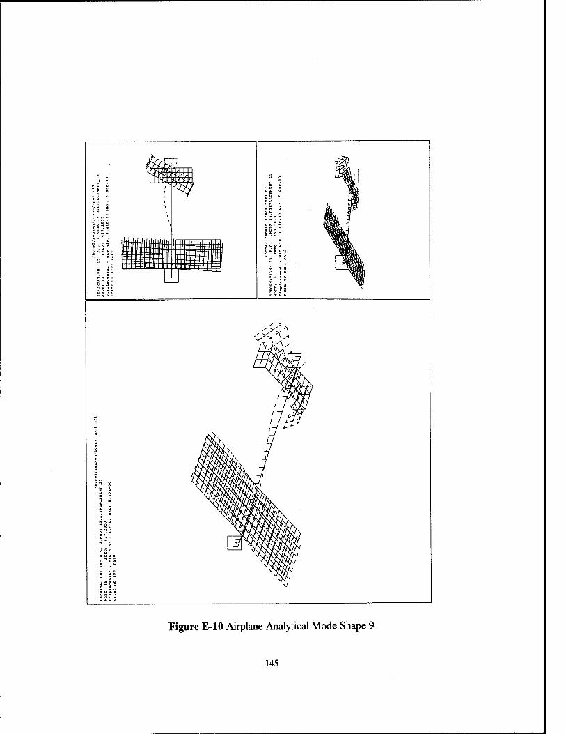
Figure E-10 Airplane Analytical Mode Shape 9
145

9M
01 adeqs spo]A[ IBOI^BUV auBidity 11-3 ajnSij
A'

Update 1-8 Design Variables, 8 Frequencies (Modes 2 + 9 omitted)
Update 2-10 Design Variables, 8 Frequencies (Modes 2 + 9 omitted)
Update 3-7 Design Variables, 9 Frequencies (Mode 9 omitted)
Update 4-5 Design Variables, 10 Frequencies
AIRPLANE MODEL OPTIMIZATION
FREQUENCY COMPARISON
EXPERIMENTAL ORIGINAL UPDATE1 UPDATE2 UPDATE3 UPDATE4 103.906 96.7507 103.23 103.068 102.563 104.081 128.125 126.072 134.18 134.289 133.197 128.326 140.625 135.637 140.76 140.695 140.29 131.579 223.047 217.966 228.13 228.594 228.445 220.362 272.266 268.562 279.77 281.173 282.574 286.383 335.156 293.406 322.9 324.807 320.417 325.954 355.469 336.579 352.1 355.239 354.135 356.173 383.984 361.009 381.03 382.403 380.726 373.172 404.297 416.758 434.63 434.55 433.12 404.904 553.125 518.864 529.25 533.166 548.772 553.945
PERCENTAGE ERROR ORIGINAL UPDATE1 UPDATE2 UPDATE3 UPDATE4
-6.88632 -0.65059 -0.8065 -1.29251 0.168421 -1.602341 4.725854 4.810927 3.958634 0.156878 -3.547022 0.096 0.049778 -0.23822 -6.43271 -2.277995 2.278892 2.48692 2.420118 -1.20378 -1.360434 2.756128 3.271433 3.786003 5.185003 -12.45689 -3.6568 -3.08782 -4.39765 -2.74559 -5.314106 -0.94776 -0.0647 -0.37528 0.198048 -5.983322 -0.7693 -0.41174 -0.84847 -2.81574 3.08214 7.502653 7.482865 7.129165 0.150137
-6.194079 -4.31638 -3.60841 -0.78698 0.148249
Average error (abs) 4.870465 2.770037 2.608108 2.523305 1.920456 MAC Sum 9.4293 9.4991 9.508 9.5112 9.5734
Table E-l Airplane Update Frequency Comparison
147

148

APPENDIX F. COMPOSITE BEAM TEST DATA
Both the undamaged and damaged composite beams were tested to obtain the
experimental dynamic responses. The excitation force was applied at 25 points along the
beam. These points corresponded to locations of finite element model nodes. Figure F-l
depicts the data point locations. Figures F-2 through F-10 are the first nine mode shapes
for the damaged beam as determined from the experimental data and IDEAS software.
149

Figure F-l Composite Beam Excitation Points
150

X
'S >- cJ 4 3 t
I \ ^ f
\ « \ ^ \ - \ ^ t
\o
V ( } =i (\ . 3 i \
^ 3 I \
* 3 f \
« =i t \
„ ^ S
3 f
=i f
*H-
*H« r*
r- ^ ■ r>j
fi 0 / • o =5 /
o + w oi
% r /
S -H / < a •■
X ^ / < B /
rH in *3> o o s i J vo Cd
• o\ r-J CD O O M VO ■v. VD VO
{N CO ■• /in « N z / S I E H -< S p » •■ O O EH
/ ^ M H <: ps i i PS S *<
O [b D<
/ ' s u. z o w O H K w E" / EH O < tU I 5 i < m EC O / S ta / PS ■• *3 W / O W W E / 5 En Q U < ' i Ed O U PS a E < fc
Figure F-2 Composite Beam Experimental Mode Shape 1
151

Zi\
Z adteqg apoj\[ |Bju9uiu9dxg uresg 9jisodui03 g-j ajnSij
s
/ >- cJ - /
H i /
S V
/ t
/ S i
/ % ■ i
f
% ■
\ * f
\ ^ i
\ * I
% f \
r- vo o a>
■ ID O O \
0. co a • Q
%
i/78 . 85377
, 85377
7 . 18E
+ 04 MAX:
1
1
DEFORMATION: 3 1-3:DAM22J
MODE: 31 FREQ: 78 .
ACCELERATION
- MAG MIN:
FRAME OF REF: PART
/ ^
1

Figure F-4 Composite Beam Experimental Mode Shape 3
153

tel
j7 sdBqs spojA[ iBjusuiusdxg ureag 9jisoduio3 g-^ ajnSij
in in oj in
O w w S fc, Q U < w o u cc

X
% >- tJ
N. % t
^ 1 \
n t \
% * )
% /
/%
( * t
% t
\ % i
% \
% f )
M
% f J
r-
% \/
■ VD /" o o / % ■
•• o
B ■ ' % ■
< O) P
X % i E
\% \ O O T CO Ol o % f\
M 00 ■■ M r-i Z % t \ S M < E P -•
>« w < cd % ) i « E <
^ ' % i J H O W O H K H En E-< -a- < (L. y/% \ < m K O
DEFO
MODE
ACCE
FRAM
% t
F igur e F-6 Composite Beam Experimental Mode Shape 5
155

9SI
9 acfeijs spop\[ jBjuauiuadxg uresg 9jisoduio3 /,-j ajnSij
in co •-» • n m o M n ■• IN in 2 S M < E Q «
E-t m rtj [ij
O 6a H H
- tj

X 1 % > fcj
^^\ *»
% ^1
n % J
j
^ % f * 3 i
\. " \H i
,, =5 ^\ * =j i y
« *5 s j/
S<
/ ** ': /
*\ ■
\ V ^ •
U3 oo 3 : ^\ (*i
\o in o
in o =5 f J • +
o w o a\ ^ i J
0. *3* E < ■• m Q X <
E
IM O f H \
w r- o Of)"»
. S ■
m r- r-] o •■ CN r- H
X ! E H < s Q » •• O O H ^ oo W < Pi f >. i BS E <
to b cu m i
s E In
£ O W O H B; M EH EH v> < h < n pj O S W OS ■- t-3 W O H fa E / 3 ft« Q U < f
W O U PC O E < tu
Figure F-8 Composite Beam Experimental Mode Shape 7
157
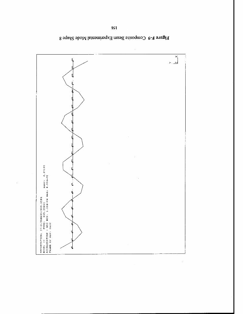
8£I
8 adBqs spopM lejirauoradxg ureag 9}isodui(>3 6-j sjnSij
X 1
3 ^^ > tJ r
\ s i
V s i
;; ^ t >.
0 ' ^ * =1 t j/
s^> 1 ** F
1 L ^ f
N. » \j ■
» 3 i ^l
„ =5 f 3
>^ " I ^ f
01 en 1 " I ^ ■
r-
o in \o
o
■■ w 0. m
< ■ % i N Q co
X \ e V < S
10
in o (M H +
• VD W in CO rH O 1/1 (N / \ en rj
in in (N O ■• \ "> CM <T\ 2 V ^ S H < E P •• ■• a o ^ ^ oi W < pi ^v
i « 2 < [-fa Cn m i %
2 fa Z o w o H pi H E* E-< r- < fa < m oi O a w rt » j a o w w s ^ % fa Q U flj ^ w o o a: Q S < fa

X.
^ >- cJ ^^Si
5 y « 3 k/
I * r
1 o I ^ ;
% : >. . s y ,. "\ F ./
/" 1 ^ f
" I % s
% r\.
„ =i y „ ^ i >/
■<*
r- o\
/ ^ ■ to ** ■ in / 2
o o t s : W
•• r- o> <-l E • < r- Q
X ^ f } < » E
o s t //
<N r- w *H PI rH
^B y/ S :
in *JI «eji
tN CN M rH •• / ui s «-• a \ s ■ 4 H
Q E
o O O E-- <H W < PS
i « E < co fc Cu
B U, ? y a o w O H K M t* t< co < fc, H iX < n a: o E W EC -- J W O W W E •^ % ft. P u < s W O U Bi a s < fc
Figure F-10 Composite Beam Experimental Mode Shape 9
159

160

APPENDIX G. STEEL BEAM SPECIFICATIONS
A. PHYSICAL DIMENSIONS AND PROPERTIES
A steel beam was used to verify the damage localization procedure. The
dimensions and the mass of the beam were measured. The original Young's modulus was
assumed to be equal to a standard value for steel. The beam orientation for the
simulations was as depicted in Figure G-l. The degrees of freedom for the beam were
vertical translation, upward in the figure, and rotation around a vector out of the plane of
the page.
n f I
I L I w
L = 3.98 feet D = 0.625 inches W = 1.125 inches
Figure G-l Steel Beam
The original physical properties assumed for the beam were:
Young's modulus E = 30 e 6 PSI mass density p = 0.00072 lbf-sec2/in4
Young's modulus was updated using the optimization procedure and comparison to the
undamaged beam's dynamic response. The updated value was:
Young's modulus E = 28.61 e 6 PSI
B. DYNAMIC RESPONSE
The damaged beam was tested to obtain the experimental dynamic
responses. The excitation force was applied at 25 points along the beam. These points
161

corresponded to locations of finite element model nodes. Figure G-2 depicts the data point
locations. Figures G-3 through G-l 1 are the first nine mode shapes for the damaged beam
as determined from the experimental data and IDEAS software.
162

X
1 >J % t
%
3 ■
% F
% f
% i
% i
■
■
■
* r
r
■
%
i
■
%
% ■
%
Figure G-2 Steel Beam Excitation Points
163

t9T
I adBqs spopM pnuaiuusdxg ureag pajs £-f) »JinSij

Figure G-4 Steel Beam Experimental Mode Shape 2
165

991
£ admjs 9po]A[ pmisuiusdxg ureag psjs S~D a-mgitf

X 1
^ F / >- bJ
„ =i i /
»
/ 3 F
3 F
1
\ ' ^ ■
\ \ ^ •
% F\
„ =?
S
CN 3 }
% F J
CN
/ *■ F
,_, a\ <N ( ** \
*-< <?,
O U) 1 o
- o j =i ■
o + \ w
\ ^ \ S rH «fl ■ < V
E . IN O % i \
T-t H o no r- in a> o -«. CN % F \ < • n \ S «H t-l o •• Q in s % i J CM M
m B / w ■• •• O U E^ % -<* a < K i J " Pä S < /
r^ fci ß*
Z 6. % ■/
a o w O H K
FT" t- < tu /% ■
< r- o: O E W K •• J W , O W M £ / % b Q U < F
W O U « Q B < fc
Figure G-6 Steel Beam Experimental Mode Shape 4
167

89T
g adeqs spop\[ pjjusumadxg uresg psjs Z,"D wnSij
< r- cC O
UNS Q U < O U Oi

v> w < «:
< r- en o
o H w s fa Q o < w o u oi Q K < fa
Figure G-8 Steel Beam Experimental Mode Shape 6
169

OZ.I
i sdBiis 3popM pnusumadxg ureag pajs 6~3 »-»nSij

Figure G-10 Steel Beam Experimental Mode Shape 8
171

ZL\
6 adeqs apop\[ leiusiuusdxg ureag pais ll"9 »jnSij

APPENDIX H. COMPUTER CODE
The following is a list and a brief description of MATLAB routines employed in
this thesis. The different problems used similar routines modified to account for the test
piece specifics and the application:
• FEMOD.M - develops finite element model and solution for a beam. Used to develop
the beam finite element models and the simulated experimental data.
• GLOOPT.M - runs optimization routine for model updating and returns results. This
program can be modified to run for the beam or any other model.
• DVMAT.M - develops the 2-level factorial combination matrix.
• OPTBEAM.M - inputs optimization process parameters such as limits and search
method.
• OBJVAL.M - contains the objective function and constraints for optimization.
• CHECKWNM - calculates updated model natural frequencies and mode shapes for
the beam trials for solution evaluation.
• CBLOC.M - divides designated region into sectors and runs localization routine for
each sector.
• MODCOMP.M - calculates the Modal Assurance Criteria for active modes.
• DIRECTM - does direct pseudo-inverse solution for the steel beam damage case. It
also contains the reduction/expansion logic.
The codes are included in the following pages.
173

FEMOD.M
% develops finite element model for a beam
function [omega,T,gamma]=femod(dv)
nel=8; nn=nel+l; % nn - number of nodes dof=nn*2; % dof - number of degrees of freedom
% input beam dimensions
lt=10; w=3; d=10;
% calculate needed parameters
le=lt* 12/nel; % le - element length ar=w*d; % ar - cross sectional area ve=ar*le; % ve - element volume Iner=w*dA3/12; % Iner - moment of Inertia
% Construct geometric properties matrices
kel=[12 6*le -12 6*le; 6*le 4*leA2 -6*le 2*leA2; -12 -6*le 12 -6*le; 6*le 2*leA2 -6*le 4*leA2];
ke=(Iner/leA3)*kel; mel=[156 22*le 54 -13*le;
22*le 4*leA2 13*le -3*leA2; 54 13*le 156 -22*le; -13*le-3*leA2 -22*le 4*leA2];
me=(ve/420)*mel;
% construct global matrices
kglo=zeros(dof,dof); mglo=zeros(dof,dof);
% properties for the different elements (assumed homogenous)
forj=l:nel
174

mod(j)=dv(l); rhoG)=dv(2);
. end
% designate element connectivity
for i=l:nel con=i+l; cl=(i*2)-l; c2=con*2; kglo(cl :c2,cl :c2)=kglo(cl :c2,cl :c2)+mod(i)*ke; mglo(cl :c2,cl :c2)=mglo(cl :c2,cl :c2)+rho(i)*me; end
% set boundary conditions - zero the matrix elements which are % constrained. Beam is cantilevered.
kact=kglo(3: dof, 3: dof); mact=mglo(3 :dof,3 :dof);
% solve for natural frequencies and mode shapes
[phi,lbd]=eig(mact\kact); forj=l:dof-2;
lambda(j)=lbdG,j); end
freqs=(sqrt(lambda)); [wn,I]=sort(freqs); forj=l:dof-2;
shnorm(:,j)=phi(:,Iö)); end
mtil=shnorm,*mact*shnorm; fori=l:dof-2;
alpha(i)=l ./sqrt(mtil(i,i)); shapes(:,i)=shnorm(:,i)*alpha(i); end
% compute sensitivities and Cauchy ratio equivalent
numdv=2*nel; sens=zeros(dof-2,numdv); gamma=zeros(dof-2,numdv);
175

counter=l; fork=l:numdv
tm=zeros(dof,dof); tk=zeros(dof, dof); ifcounter<=nel
con=counter+l; cl=(counter*2)-l; c2=con*2; tk(cl:c2,cl:c2)=ke;
else r=counter-numdv/2; con=r+l; clKr*2)-l; c2=con*2; tm(cl:c2,cl:c2)=me; end
tkact=tk(3:dof,3:dof); tmact=tm(3: dof, 3: dof); forg=l:dof-2
% sensitivity calculation
mat=tkact-wn(g)A2 *tmact; delw=shapes(:,g)'*mat*shapes(:,g); sens(g,k)=sens(g,k)+delw;
% Cauchy ratio calculation
forr=l:dof-2 ifr=g
gam=0; else
gam=-(shapes(:,r)'*mat*shapes(:,g))A2/((wn(g)A2- wn(r)A2)*delw);
end gamma(g,k)=gamma(g,k)+gam;
end mat=zeros(dof-2,dof-2);
end counter=counter+1;
end
omega:=wn(l:4); T=sens(l:4,:);
176

GLOOPT.M
% Perform multiple iterations of optimization program for different combinations % of design variables. This particular code is set up to do the 8 element beam problem % with up to 16 design variables.
global size block Tb dvO dvsc n dwect omega measom prop
diary
% Determine Design variable matrix for iterations.
n=4; block=16/n; bimat=dvmat(n);
% Calculate FE model and Experimental Values
prop=[10e6 .000254]; [omega, T,cauchy]=femod(prop); load moddat omega=omega prodv=[9.2e6 .000254]' [measom,measphi]=expmod(prodv); measom=measom startpt=[10e6 .000254]';
% solve optimization problem for each set of design variables
count=n/2; nrow=2An-l; fori=l:nrow
dv=zeros(n,l); stpt=zeros(n,l); dwect=bimat(i,:) Tact=T; cauchyact=cauchy; ckdv=prodv;
% generate dv vector and initial values for the iteration. Also eliminate terms to account % for which design variables are in used
forj=l:n ifj<=count
177

else
ifdwect(j)=l dv(j)=prop(l); stpt(j)=startpt( 1 )-prop( 1);
else dv(j)=0;
end
ifdwect(j)=l dv(j)=prop(2); stpt(j)=startpt(2)-prop(2);
else dv(j)=0;
end end
end
% eliminate unneeded dv information for the iteration
forj=n:-l:l ifdwect(j)=0
dvö)-[]; stpt(j)=[]; Tact(:,G-l)*block+l:j*block)=[]; cauchyact(:,(j-l)*block+l :j*block)=[]; ckdv(j)=[];
end end
% scale design variables
scale=min(dv)/max(dv); size=length(dv); size l=length(Tact( 1,:)); sc=zeros(sizel); for j=l: size 1
sc(jj)=i; end for j=l: size
ifdv(j)/prop(l)=l for k=(j-l)*block+l :j*block
sc(k,k)-scale; end
end end
178

Tb=Tact*inv(sc);
% scale design variable vector and starting point vector
dvsc=zeros(size); for j=l: size
ifdv(j)/prop(l)=l dvsc(j,j)=scale;
else
dvscQJH; end
end dvO=dvsc*dv; deldvO=dvsc*stpt; diary
% enter constrained optimization routine
[optdv,senvexp,senveig,eigvexp,mac]=optbeam(dv,deldvO,measphi); diary
% develop vector to calculate Cauchy ratio
ddv=zeros(size*block, 1); for 1=1: size
forj=l:block start=(l-l)*block; ddv(start+j)=optdv(l)-dv(l);
end end
% print out solution data
optdv=optdv data=[senvexp senveig eigvexp] % this is frequency comparison data pctdiflE=(optdv-ckdv)./ckdv* 100 macsum=sum(mac); for j=l :length(ddv)
cauchyrat(:j)=cauchyact(:,j)*ddvö); end
ratio=max(abs(cauchyrat( 1:4,:))); dvposit=l; forj=l:n
ifdwect(j)=l
179

output(ij)=optdv(dvposit); dvposit=dvposit+1;
else output(ij)=0;
end end output(i,n+l)= =macsum;
end diary off
180

DVMAT.M
% develops matrix to track design variable combinations. Returns a matrix with ones % and zeros in a binary type code.
function [bimat]=dvmat(n)
nrow=2An; bimat=zeros(nrow,n); for i=l:n
counter=2A(i-l); part 1 =zeros(counter, 1); part2=ones(counter, 1); fill( 1: counter, 1 )=part 1; fill(counter+l :counter*2, l)=part2; size=length(fill); for j=1: nrow/(2 * counter)
bimat((j-1 )*size+1 :j * size,i)=fill; end
end bimat(l,:)=[];
181

OPTBEAM.M
% provides information needed by the optimization process
function[optdv,senvexp,senveig,eigvexp,mac]=optbeam(dv,deldvO,expsh)
global dvsc measom newom prop
% sets limits and defines information for the constrained optimization routine
U=-.l*dv; ul=.l*dv; options=[]; options(l)=l; options(2)=le-8; options(3)=le-8; options(6)=2; options(14)=1000;
% enters the optimization routine
[optdel]=constr('objvar,deldvO,options,ll,ul);
% scales the solution back to original basis and adds to original value
optdel=dvsc\optdel; optdv=dv+optdel;
% updates FEM
[eigomega,newphi]=checkwn(optdel,prop);
% compares frequencies Sensitivity update vs experimental, Sensitivity update vs % eigen re-solve, and eigen re-solve vs experimental (percentage basis)
senvexp=max(abs((measom-newom)./measom))* 100; senveig=max(abs((eigomega-newom)./eigomega))* 100; eigvexp=max(abs((measom-eigomega)./measom))* 100;
% calculates MAC
[mac]=modcomp(expsh,newphi);
182

OBJVAL.M
% computes objective function and constraint values
function [value, con]=objval(deldv)
global size block Tb newom measom dvO omega
% expands a single dv value up to number of linked variables, i.e. IE value up to 8 % elements
m=length(deldv); ddv(m*block, l)=zeros; for i=l:m
forj=l:block ddv((i-l)*block+j)=deldv(i);
end end
% calculates sensitivity update
diff=Tb*ddv; newom=sqrt(omega.A2+diff);
% calculates Objective function
subval 1 =5 * sum(abs((measom-newom)./measom)); subval2=block*sum(abs(deldv./dv0)); value=subval 1 +subval2;
% calculates constraint value (none in this case)
con=[];
183

CHECKWN.M
% calculates updated frequencies and mode shapes based on optimization solution
function [wnnew,shapes]=checkwn(deldv,dv)
global n block dwect
% define beam parameters (same as baseline model
nel=8; nn=nel+1; % nn - number of nodes dof=nn*2; % dof - number of degrees of freedom lt=10; w=3; d=10;
% expands dv vector up to fill 16 values ( 8 for E, 8 rho)
fori=l:n forj=l:block
ifi<=n/2 num=(i-1 )*block+j; mod(num)=dv(l);
else num=(i-n/2-l)*block+j; rho(num)=dv(2);
end end
end
% adds change in design variables to original values
count=l; for w=l :n
if dwect(w)=l ifw<=n/2
for j=(w-l)*block+l :w*block; mod(j)=mod(j)+deldv(count);
end else
q=w-n/2; for j=(q-l)*block+l :q*block;
184

rho(j)=rho(j)+deldv(count); end
end
count=count+l; end
end
le=lt* 12/nel; % le - element length ar=w*d; % ar - cross sectional area ve=ar*le; % ve - element volume Iner=w*dA3/12; % Iner - moment of Inertia
% calculates elemental mass and stiffness matrices
ke=[12 6*le -12 6*le; 6*le 4*leA2 -6*le 2*leA2; -12 -6*le 12 -6*le; 6*le 2*leA2 -6*le 4*leA2];
ke=(Iner/leA3)*ke; me=[156 22*le 54 -13*le;
22*le 4*leA2 13*le -3*leA2; 54 13*le 156 -22*le; -13*le-3*leA2 -22*le 4*leA2];
me=(ve/420)*me;
% assembles global matrices
kglo=zeros(dof,dof); mglo=zeros(dof,dof); ori=l:nel
con=i+l; cl=(i*2)-l; c2=con*2; kglo(cl :c2,cl :c2)=kglo(cl :c2,cl :c2)+mod(i)*ke; mglo(cl :c2,cl :c2)=mglo(cl :c2,cl :c2)+rho(i)*me;
end
% define boundary conditions
kact=kglo(3:dof,3:dof); mact=mglo(3 :dof,3 :dof);
% solve eigen problem
185

[phi,lbd]=eig(mact\kact); forj=l:dof-2;
lambdaö)=lbdö,j); end
freqs=(sqrt(lambda)); [wn,I]=sort(freqs); forj=l:dof-2;
shnorm(:,j)=phi(:,I(j)); end
mtil=shnorm' * mact * shnorm; fori=l:dof-2;
alpha(i)=l ./sqrt(mtil(i,i)); shapes(:,i)=shnorm(:,i)*alpha(i); end
wn=wri: wnnew=wn(l:4);
186

CBLOC.M
% Perform multiple iterations of optimization program for composite beam % to localize damage
global Tbca dv anfreq exfreqd newfreq
% Call model data
load cb8; % composite beam data file anfreq=omega/2/pi; load('exfreqd. dat') load cddamdat; % damaged composite beam data file
% solve optimization
dv=6.7576e6; count=length(anfreq); c=8*piA2;
% convert sensitivities from delta lambda to delta frequency
for i=l: count Tb(i,:)=T(i,:)/c/anfreq(i); end
% Enter the section of the beam to be investigated % there must be at least 3 elements
le=input(Enter the first element of the region of interest -'); re=input('Enter the last element of the region of interest -');
% sum the sensitivities for the three sections
numel=re-le+l; step=fix(numel/3); leftover=rem(numel,3); ifleftover=0
lb(l)=le; lb(2)=le+step; rb(l)=lb(2)-l; lb(3)=lb(2)+step; rb(2)=lb(3)-l; rb(3)=re;
187

elseifleftover=l lb(l)=le; lb(2)=le+step; rb(l)=lb(2)-l; lb(3)=lb(2)+step+l; rb(2)=lb(3)-l; rb(3)=re;
elseifleftover=2 lb(l)=le; lb(2)=le+step+l; rb(l)=lb(2)-l; lb(3)=lb(2)+step; rb(2)=lb(3)-l; rb(3)=re;
end lb(4)=le; rb(4)=re;
% sum elements of sensitivity matrix for the three sections and % the whole sector
temp=Tb(:,lb(l):rb(l))'; iflb(l)=rb(l)
Tbc(:,l)=temp'; else
Tbc(:,l)=sum(temp)'; end temp=Tb(:,lb(2):rb(2))'; iflb(2)=rb(2)
Tbc(:,2)=temp'; else
Tbc(:,2)=sum(temp)'; end temp=Tb(:,lb(3):rb(3))'; iflb(3)==rb(3)
Tbc(:,3)=temp'; else
Tbc(:,3)=sum(temp)'; end Tbc(:,4)=Tbc(:,l)+Tbc(:,2)+Tbc(:,3);
% solve the optimization problem for each section
fori=l:4
188

Tbca=Tbc(:,i); deldvO=0;
% enter optimization (values the same as previous applications)
[optdv,ufreq,pctdiff,mcf]=dlopt(dv,deldvO,xshp,lb(i),rb(i));
solvec(i)=optdv; update(:,i)=ufreq; pctd(:,i)=pctdiff; modalc(:,i)=mcf; end
% print results, DV values and MAC sums
solvec=solvec modalc=modalc
% add different combinations of mode MAC's
total(l, total(2, total(3, total(4, total(5, total(6, total(7, total(8, total(9,
:sum(modalc); =sum(modalc(l
sum(modalc(5 sum(modalc(l
=sum(modalc(3 =sum(modalc(5 =sum(modalc(7 =sum(modalc(l ~sum(modalc(3
A )); :8, )); :2, )); A, )); :6, )); :8, )); :6, )); :8, ));
189

MODCOMP.M
% calculated modal assurance criterion
function [factor]=modcomp(old,new);
factor=zeros(8,l); fori=l:8
top=old(:,i)'*new(:,i); bl=old(:,i)'*oId(:,i); b2=new(:,i)'*new(:,i); factor(i)=topA2/(bl*b2);
end
190

DIRECT.M
% this function solves for design variable difference with the pseudo-inverse method
function [optdv,mcf]=direct(dv,Tbca,olshp,lb,rb)
global anfreq exfreqd aset oset Ttype mact kact compshp redshapes
% solve for dv value
delfreq=exfreqd-anfreq; optdel=Tbca\delfreq; optdv=dv+optdel;
[eigomega,mupd,kupd,upshp]=ckwn(optdel,lb,rb);
% select transformation matrix method
%[kstat,mstat,T_static]=fstatic_tam(kupd,mupd,oset,aset); [kstat,mstat,T_static]=firstam(kupd,mupd,oset,aset);
% generate shape vectors
count=length(aset); ndof=length(oset)+count;
if Ttype==l % for reduction of analytical to experimental size
compshp=olshp; [wnred,red_shapes]=shgen(mstat,kstat);
elseif if Ttype=2 % extraction method
compshp=olshp; for i=l: count
red_shapes(i, :)=upshp(aset(i),:)' end
elseif if Ttype==3 % expand experimental up to analytical size
% [kstat 1 ,mstat 1 ,T_static 1 ]=fstatic_tam(kact,mact,oset,aset); [kstat 1 ,mstat 1 ,T_static 1 ]=firstam(kact,mact,oset,aset); compshp=upshp; phi_exp=T_staticl *olshp;
191

start=ndof-count; for i=l: count % unpartitioning shape vector
red_shapes(aset(i), :)=phi_exp(start,:); t=(i-l)*3; red_shapes(aset(i)+l :aset(i)+3,:)=phi_exp(t+l :t+3,:); end
red_shapes(99,100)=[];
end
eig=eigomega/2/pi; eigvexp=(eig-esfreqd)./exfreqd* 100;
% calculating MAC
[mcf]=modcomp(compshp,red_shapes);
192

APPENDIX I. IDEAS CONVERSION INFORMATION
The IDEAS simulation software provides finite element modeling capability with a
graphic end. The program allows the user to build and solve models. To allow for
conversion between IDEAS and other software some conversions were necessary. The
following will provide a walk through of those measures.
A. SENSITIVITY CONVERSION
The equation developed for frequency sensitivities in Chapter II, Equation (2.11),
defines the frequency sensitivity as a change in lambda per change in design variable. This
was the method used in the MATLAB code. IDEAS on the other hand computes the
frequency sensitivity on a change in frequency per change in design variable basis. The
conversion from one to the other is developed as follows by substituting for lambda:
a _a(w)'.=^^= * (u) cDV SDV SDV v 'cDV
= 87t2f-—7 (1.2) aDV aov
This allows the conversion of sensitivities on a lambda basis to a frequency basis. The
other issue is the units of the denominator. IDEAS outputs sensitivities in the unit system
designated within the model file, so if English units are designated the output file will be in
English units.
B. MODE SHAPE NORMALIZATION AND MODAL MASSES
IDEAS normalizes the output mode shapes in a different fashion than MATLAB.
MATLAB normalizes mode shapes so that the magnitude of the modes shape vector is
one. For the models used in this thesis, English units were used, so that the nominal units
193

of the mode shape vector were inches for deflection and radians for rotation. Modal mass
is in lbf*sec2/in. IDEAS normalizes mode shapes so that the magnitude of the largest
single element in the modal matrix is one. The program outputs the modes shapes in
metric units, so that deflections are in meters and rotations are in radians. In order to
convert MATLAB data to the same format as IDEAS data the following procedure is
used:
• convert active mass matrix from lbf*sec2/in to kg
lbf * sec2 ,12in. 14.159kg (u)
in ft slug
• convert translations in modal matrix from inches to meters (odd rows of
matrix)
in,25taa,_jn_ (I4)
in 100cm
• renormalize mode shape matrix so that largest term is one
max^i)
• Calculate modal mass with renormalized modal matrix and mass matrix
194

LIST OF REFERENCES
1. Flanigan, C.C., "Test Analysis Correlation Using Design Sensitivity and Optimization - Does It Work?", Society of Automotive Engineers, Inc., 1988.
2. Luber, W., Sensburg, 0., "Identification of Errors and Updating in Analytical Models Using Test Data", 13th International Modal Analysis Conference, Nashville, TN, 1995, pp. 407-413.
3. Dascotte, E., Stroble, J., Hua, H., "Sensitivity-Based Model Updating Using Multiple Types of Simultaneous State Variables", 13th International Modal Analysis Conference, Nashville, TN, 1995, pp. 1035-1040.
4. Vanderplaats, G., Numerical Optimization Techniques for Engineering Design, pp. 79, 88, 93, 97-100, McGraw-Hill, Inc., 1984
5. Allemang, R.J., Brown, D.L., "A Correlation Coefficient for Modal Vector Analysis", 1st International Modal Analysis Conference, , 1982, pp. 110-116.
6. Barker, T.B., Quality by Experimental Design, pp. 51-60, Marcel Dekker, Inc., 1994.
7. Hemez, F.M., Farhat, C, "Structural Damage Detection Via a Finite Element Model Updating Methodology", Modal Analysis, The International Journal of Analytical and Experimental Modal Analysis, Volume 10, Number 3, July 1995.
8. Crema, L.B., Castellani, A., Coppotelli, G., "Generalization of Non-destructive Damage Evaluation Using Modal Parameters", 13th International Modal Analysis Conference, Nashville, TN, 1995, pp. 429-434.
9. Lam, H.F., Ko, J.M., Wong, C.W., "Detection of Damage Location Based on Sensitivity Analysis", 13th International Modal Analysis Conference, Nashville, TN, 1995, pp. 1499-1505.
10. Zongbou Li, Houghton, J.R., "Damage Location in Structures Using Vibration Data and It's Sensitivity to Measurement Errors", 13th International Modal Analysis Conference, Nashville, TN, 1995, pp. 1418-1424.
11. Brandon, J.A., "Second-order Design Sensitivities to Assess the Applicability of Sensitivity Analysis", Journal of the American Institute of Aeronautics and Astronautics, Volume 29, Number 1, January 1991, pp. 135-139.
12. Guyan, R.J., "Reduction of Stiffness and Mass Matrices", Journal of the American Institute of Aeronautics and Astronautics, Vol. 3, February 1965, p. 380.
195

13. O'Callahan, J., "A Procedure for an Improved Reduction System (IRS) Model", 7th International Modal Analysis Conference, Las Vegas, NV, 1989.
14. Campbell, M., "Structural Damage Detection Using Frequency Domain Error Localization", Master's Thesis, Naval Postgraduate School, December 1994.
15. IDEAS Master Series 2.1 Manuals
196

INITIAL DISTRIBUTION LIST
No. Copies
1. Defense Technical Information Center 2 8725 John J. Kingman Rd, STE 0944 Ft. Belvoir, VA 22060-6218
2. Library, Code 13 2 Naval Postgraduate School Monterey, California 93943-5101
3. Professor J.H. Gordis, Code ME/GO 3 Department of Mechanical Engineering Naval Postgraduate School Monterey, California 93943
4. Naval Engineering Curricular Office 1 Code 34 Naval Postgraduate School Monterey, California 93943-5000
5. LCDR Jay A. Renken, USN 2 Naval Sea Systems Command (PMS-303) 2531 Jefferson Davis Highway Arlington, VA 22242-5160
197