D I La (Y C'OP

R NAVAL POSTGRADUATE SCHOOL, Monterey, California

A 4,

'7"CR ADg

THESIS

BUBBLE PRODUCTION BY BREAKING WAVES

by

Albert C. Daniel Jr.

December 1989

Thesis Advisor Herman Medwin

Approved for public release; distribution is unlinjited.

DTrICELECTEM AYt 2 11990"

Unclassifiedsecurity classification of this page

REPORT DOCUMENTATION PAGElIa Report Security Classification Unclassified Ib Restrictive Markings

2a Security Classification Authority 3 Distribution Availability of Report2b Declassification Downgrading Schedule Approved for public release; distribution is unlimited.4 Performing Organization Report Number(s) S Monitoring Organization Report Number(s)6a Name of Performing Organization 6b Office Symbol 7a Name of Monitoring OrganizationNaval Postfraduate School (If applicable) 33 Naval Postraduate School6c Address (clty, state, and ZIP code) 7b Address (cly, state, and ZIP code)'Monterey. CA 93943-5000 Monterey, CA 93943-5000Sa Name of Funding Sponsoring Organization Sb Office Symbol 9 Procurement Instrument Identification Number

(if applicable)Sc Address (clt, state, and ZIP code) 10 Source of Funding Numbers.. ,_Program Element No Project No I ask No I Work Unit Accession No

II Title (Include securlN classlilcadon) BUBBLE PRODUCTION BY BREAKING WAVES12 Personal Author(s) Albert C. Daniel Jr.13a Type of Report 13b Time Covered 14 Date of Report (year, month, day) 15 Page CountMaster's Thesis From To December 1989 6316 Supplementary Notation The views expressed in this thesis are those of the author and do not reflect the official policy or po-sition of the Department of Defense or the U.S. Government.17 Cosati Codes IS Subject Terms (continue on reverse If necessary and Identify by block number)Field Group Subgroup Bubble production density

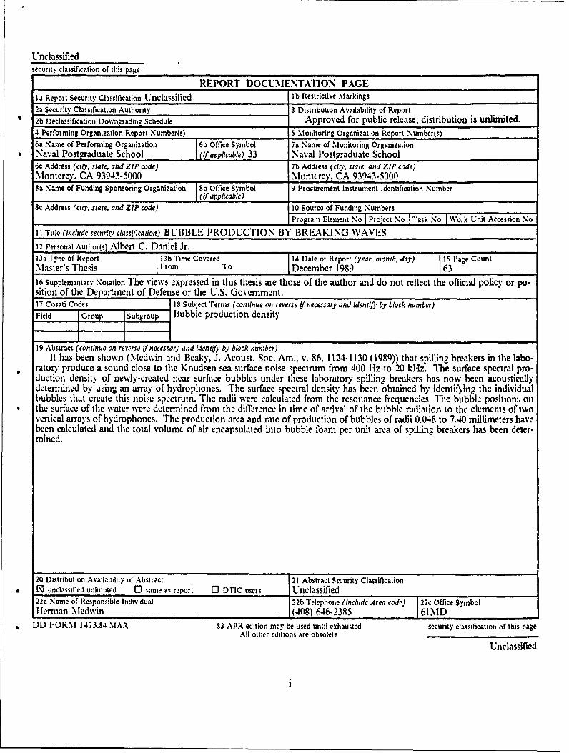
19 Abstract (continue on reverse ti necessary and identify by block number)It has been shown (Medwin and Beaky, J. Acoust. Soc. Am., v. 86, 1124-1130 (1989)) that spilling breakers in the labo-

ratory produce a sound close to the Knudsen sea surface noise spectrum from 400 Hz to 20 kI-z. The surface spectral pro-duction density of newly-created near surface bubbles under these laboratory spilling breakers has now been acousticallydetermined by usig an array of hydrophones. The surface spectral density has been obtained by identifying the individualbubbles that create this noise spectrum. The radii were calculated from the resonance frequencies. The bubble positionw, onthe surface of the water were determined fron the difference in time of arival of the bubble radiation to the elements of twovertical arrays of hydrophones. The production area and rate of production of bubbles of radii 0.048 to 7.40 millimeters havebeen calculated and the total volume of air encapsulated ito bubble foam per unit area of spilling breakers has been deter-mined.

20 Distribution Availability of Abstract 21 Abstract Security Classification5 unclasified unlimited 0 same aq report - Dric users Unclassified22a Name of Responsible Individual 22b Telephone (Include Area code) 22c Office SymbolIlerman Medwin (408) 646-2385 61IMD

DD FORM 1473.si MAR 83 APR edition may be used until exhausted security classification of this pageAll other editions are obsolete

Unclassified

Approved for public release; distribution is unlimited.

Bubble Production by Breaking Waves

by

Albert C. Daniel Jr.Lieutenant, United States Navy

B.S., University of South Carolina, 1984

Submitted in partial fulfillment of therequirements for the degree of

MASTER OF SCIENCE IN ENGINEERING ACOUSTICS

from the

NAVAL POSTGRIADUATE SCHOOLDccembcr 1989

Author: GU9, 9,&- ~JQ ' 2

A\lbert C. D ,t Jr.

Approved by:

I I rnan M edwin, Thesis Advisor

4 ev A. 'stuen, ScdRae

I: on v A . A tch l, C ai m n

Engineering Acoustics Academic Committee

ii

ABSTRACT

It has been shown (Medwin and Beaky,)J. Acoust. Soc. Am., v. 86, 1124-1130

--- --89))that spilling breakers in the laboratory produce a sound close to the Knudsensea surface noise spectrum from 400 1z to 20 kHz. The surface spectral production

density of newly-created near surface bubbles under these laboratory spilling breakers

has now been acoustically determined by using an array of hydrophones. The surface

spectral density has been obtained by identifying the individual bubbles that create this

noise spectrum. The radii were calculated from the resonance frequencies. The bubble

positions on the surface of the water were determined from the difference in time of ar-

rival of the bubble radiation to the elements of two vertical arrays ofhydrophones. The

production area and rate of production of bubbles of radii 0.048 to 7.40 millimeters have

been calculated and the total volume of air encapsulated into bubble foam per unit area

of spilling breakers has been determined. "Bv bL_', p &-pc,c ,i4 '

Aoession ForNTIS GRA&IDTIC TABUnannounced 0Justificatio

DyDistribution/

Availability CodesAvail and/or

Dist Special

Witi

TABLE OF CONTENTS

I. INTRODUCTION .............................................. 1

I. BACKGROUND .............................................. 2

Ill. FACILITIES AND APPARATUS ............................... 6

IV. EXPERIM ENT ............................................... 9

A. BREAKER SPECTRUM ...................................... 9B. BUBBLE IDENTIFICATION ................................. 14

C. BUBBLE LOCATIO.N ....................................... 19

D. RATE OF BUBBLE PRODUCTION ............................ 30E. BUBBLE PRODUCTION DENSITY ............................ 36

V. COMPARISON WITH OTHER DETERMINATIONS ................ 41b

VI. CONCLUSIONS ............................................. 44

APPENDIX A. EVIDENCE OF CAPILLARY WAVES .................. 45

APPENDIX B. VOLTAGE AMPLIFIERS ............................ 50

LIST OF REFERENCES ........................................... 53

INITIAL DISTRIBUTION LIST .................................... 55

iv

LIST OF FIGURES

Figure 1. Equipment setup ........................................ 8Figure 2. Average deepwater ambient noise spectra. (Crick) ............... 11Figure 3. Anechoic tank background noise spectra ...................... 12

Figure 4.. Average noise spectrum from six breaking waves ................. 13Figure 5. Large triggering bubble from breaking wave .................... 16Figure 6. Additional smaller bubble identification .............. ......... 17

Figure 7. Small bubble identification ................................ 18Figure 8. Bubble location geometry ................................. 24

Figure 9. Bubble location technique .................................. 25

Figure 10. TinLing error due to wave height ........................... 26

Figure 11. Distribution of bubble locations ............................. 27

Figure 12. Bubble location plot ..................................... 28

Figure 13. Bubble location plot ...................................... 29

Figure 14. Average number of bubbles produced per laboratory breaker ........ 32

Figure 15. Average number of large bubbles per laboratory breaker ........... 33

Figure 16. Average number of mid-size bubbles per laboratory breaker ......... 34

Figure 17. Average number of small bubbles per laboratory breaker ........... 35

Figure 18. Average surface density of bubbles produced .................... 38

Figure 19. Average surface density of bubbles produced .................... 39

Figure 20. Volume of air encapsulation per surface area .................... 40

Figure 21. Rate of lbrmation of air bubbles in wind waves (Toba) ............. 42

Figure 22. Rate of formation of air bubbles in wind waves (Toba) ............ 43

Figure 23. Possible capillary wave positions by bubble location .............. 47

Figure 24. Photograph of capillary waves .............................. 48Figure 25. Photograph of capillary waves .............................. 49

Figure 26. Amplifier circuit diagram .................................. 51

Figure 27. Operational characteristics of the amplifier ..................... 52

v

ACKNOWLEDGEMENT

I would like to express my great appreciation to Professor Herman Medwin for hispatient guidance and for his willingness to share his valuable knowledge. It has been a

privilege to work with someone so respected in his field. Professor Jeffrey Nystuen wasparticularly helpful with his ready suggestions and observations. I would also like to

thank my wife, Sherry, for her loving support and confidence that this thesis really would

be completed.

vi

I. INTRODUCTION

The purpose of this thesis is to develop a method for the determination of the bubbleproduction density from breaking waves. The motivation for this study came from theobservation that the spectrum produced from the noise of the breaking waves in thelaboratory tank at the Naval Postgraduate School closely resembled the Knudsen seasurface spectrum of the ambient noise at sea. This development suggested that thebreaking waves experimentally produced will exhibit the same bubble characteristics asbreaking waves at sea. It is hoped that the capability of comparing the calculated bub-ble production density with the area of foam coverage monitored with satellite imagingand aerial photography will aid in acoustical and meteorological research of air/seainteractions by predicting the number and size of bubbles which may be found in the.region being studied.

The method used in this research is to utilize passive acoustics to identify individualbubbles cruated from breaking waves. The breaking of the wave, characterized by theinitial formation of a large amplitude, low frequency bubble, was used as a triggeringsource for the signal processing equipment. The location of each subsequent bubble wascalculated by using the difference in time of arrival of the noise from the bubble to thedifferent elements of a hydrophone array. The bubble production area can be measuredby positioning all the bubble locations on a grid. The rate of bubble production wasobserved to behave as an exponentially decreasing function of time. This was determinedby noting the relative time of arrival of the pressure waves from the individual oscillatingbubbles to a hydrophone array. The bubble production density and volume rate of gasentrainment were calculated from the bubble population data and the measured area ofbubble production. This technique provided information on bubble production on thesurface, a quantity which had not been directly measured in any other previous exper-imental work.

II. BACKGROUND

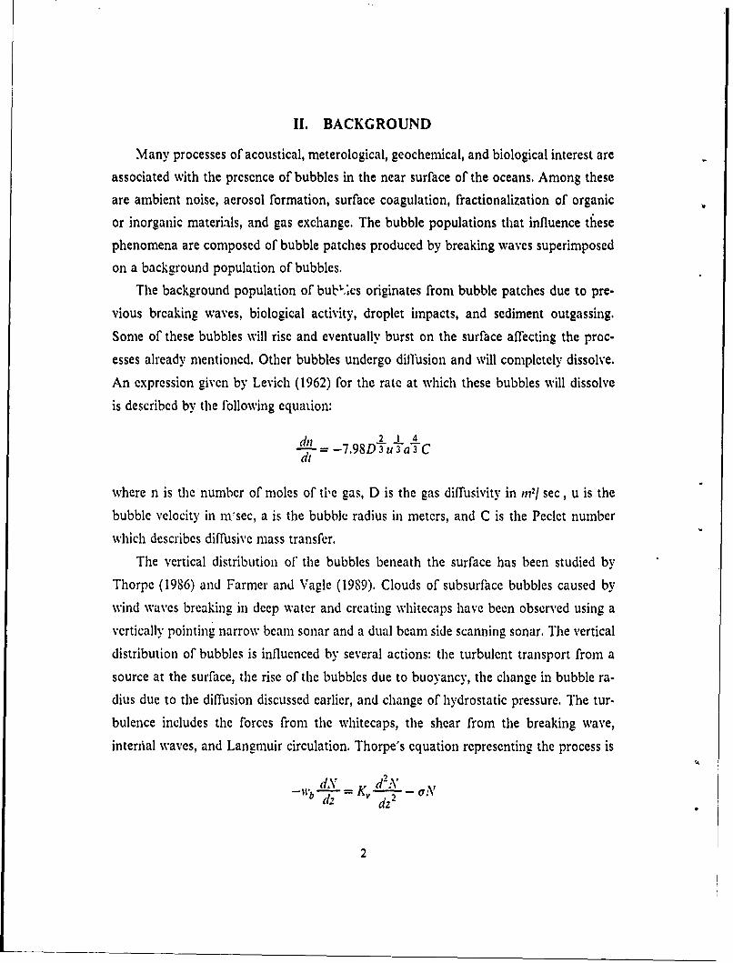
Many processes of acoustical, meterological, geochemical, and biological interest areassociated with the presence of bubbles in the near surface of the oceans. Among these

are ambient noise, aerosol formation, surface coagulation, fractionalization of organic

or inorganic materials, and gas exchange. The bubble populations that influence these

phenomena are composed of bubble patches produced by breaking waves superimposedon a background population of bubbles.

The background population of bubl cs originates from bubble patches due to pre-vious breaking waves, biological activity, droplet impacts, and sediment outgassing.

Some of these bubbles will rise and eventually burst on the surface affecting the proc-

esses already mentioned. Other bubbles undergo difflusion and will completely dissolve.

An expression given by Levich (1962) for the rate at which these bubbles will dissolve

is described by the following equation:

dn 2 1 4

7-= -7.98DTuTaTC

where n is the number of moles of tie gas, D is the gas diffusivity in ,n2/ sec , u is the

bubble velocity in nvsec, a is the bubble radius in meters, and C is the Peclet numberwhich describes diffusive mass transfer.

The vertical distribution of' the bubbles beneath the surface has been studied by

Thorpe (1986) and Farmer and Vagle (1989). Clouds of subsurface bubbles caused by

wind waves breaking in deep water and creating whitecaps have been observed using avertically pointing narrow beam sonar and a dual beam side scanning sonar. The vertical

distribution of bubbles is influenced by several actions: the turbulent transport from a

source at the surface, the rise of the bubbles due to buoyancy, the change in bubble ra-dius due to the diffusion discussed earlier, and change of hydrostatic pressure. The tur-

bulence includes the forces from the whitecaps, the shear from the breaking wave,

interfial waves, and Langmuir circulation. Thorpe's equation representing the process is

dN = -2_ aN(z . dz

2

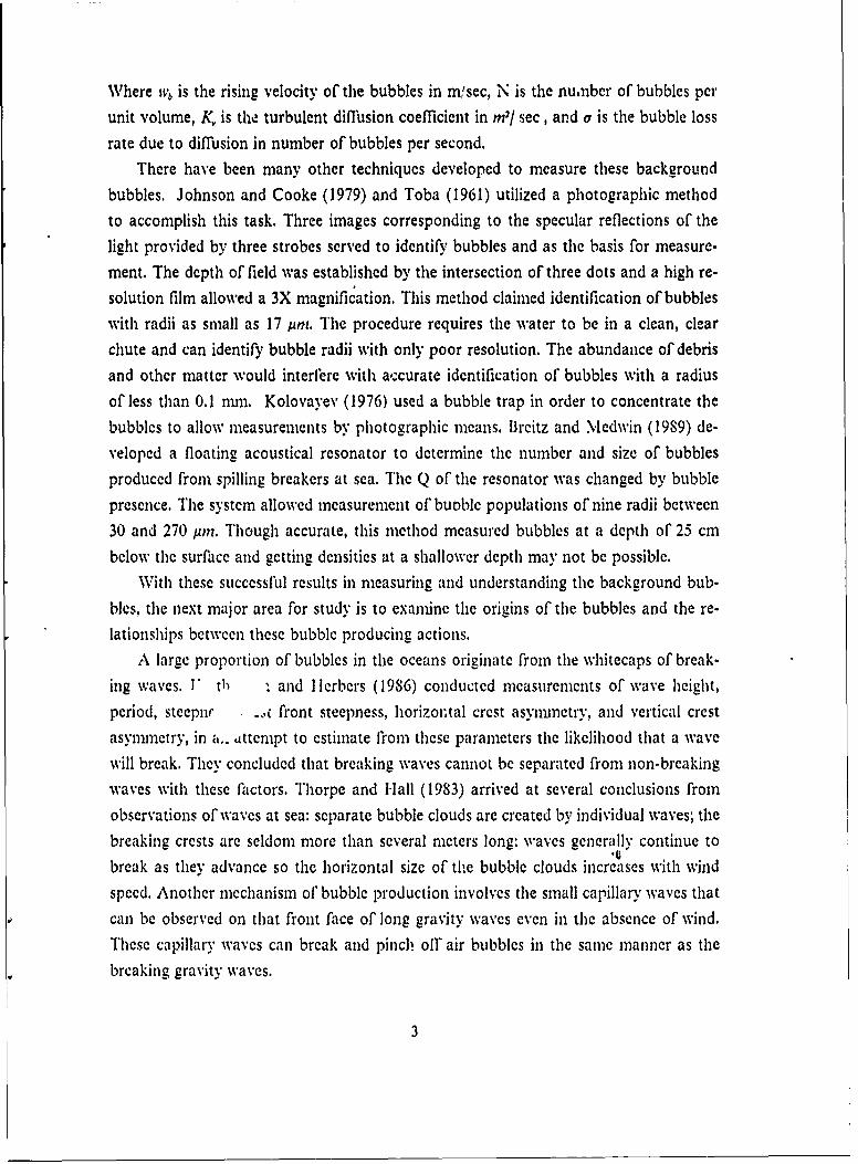
Where Wvb is the rising velocity of the bubbles in m'sec, N is the number of bubbles per

unit volume, K, is the turbulent difflusion coefficient in rn2/ see, and a is the bubble loss

rate due to diffusion in number of bubbles per second.

There have been many other techniques developed to measure these background

bubbles. Johnson and Cooke (1979) and Toba (1961) utilized a photographic method

to accomplish this task. Three images corresponding to the specular reflections of the

light provided by three strobes served to identify bubbles and as the basis for measure-

ment. The depth of field was established by the intersection of three dots and a high re-solution film allowed a 3X magnification. This method claimed identification of bubbles

with radii as small as 17 um. The procedure requires the water to be in a clean, clear

chute and can identify bubble radii with only poor resolution. The abundance of debris

and other matter would interlere with accurate identification of bubbles with a radius

of less than 0.1 nm. Kolovayev (1976) used a bubble trap in order to concentrate the

bubbles to allow measurements by photographic means. llreitz and .Medwin (19S9) de-veloped a floating acoustical resonator to determine the number and size of bubbles

produced from spilling breakers at sea. The Q of the resonator was changed by bubble

presence. The system allowed measurement of buoble populations of nine radii between

30 and 270 um. Though accurate, this method measured bubbles at a depth of 25 cm

below the surface and getting densities at a shallower depth may not be possible.

With these successful results in measuring and understanding the background bub-

bles, the next major area for study is to exanine the origins of the bubbles and the re-

lationships between these bubble producing actions.A large proportion of bubbles in the oceans originate from the whitecaps of break-

ing waves. V th . and Ilerbers (1986) conducted measurements of wave height,

period, steepnr -,c front steepness, horizontal crest asymmetry, and vertical crest

asymmetry, in a.- attempt to estimate from these parameters the likelihood that a wave

will break. They concluded that breaking waves cannot be separated from non-breaking

waves with these factors. Thorpe and Hall (1983) arrived at several conclusions from

observations of waves at sea: separate bubble clouds are created by individual waves; the

breaking crests are seldom more than several meters long: waves generally continue to

break as they advance so the horizontal size of the bubble clouds increases with wind

speed. Another mechanism of bubble production involves the small capillary waves that

can be observed on that front face of long gravity waves even in the absence of wind.

These capillary waves can break and pinch off air bubbles in the same manner as the

breaking gravity waves.

3

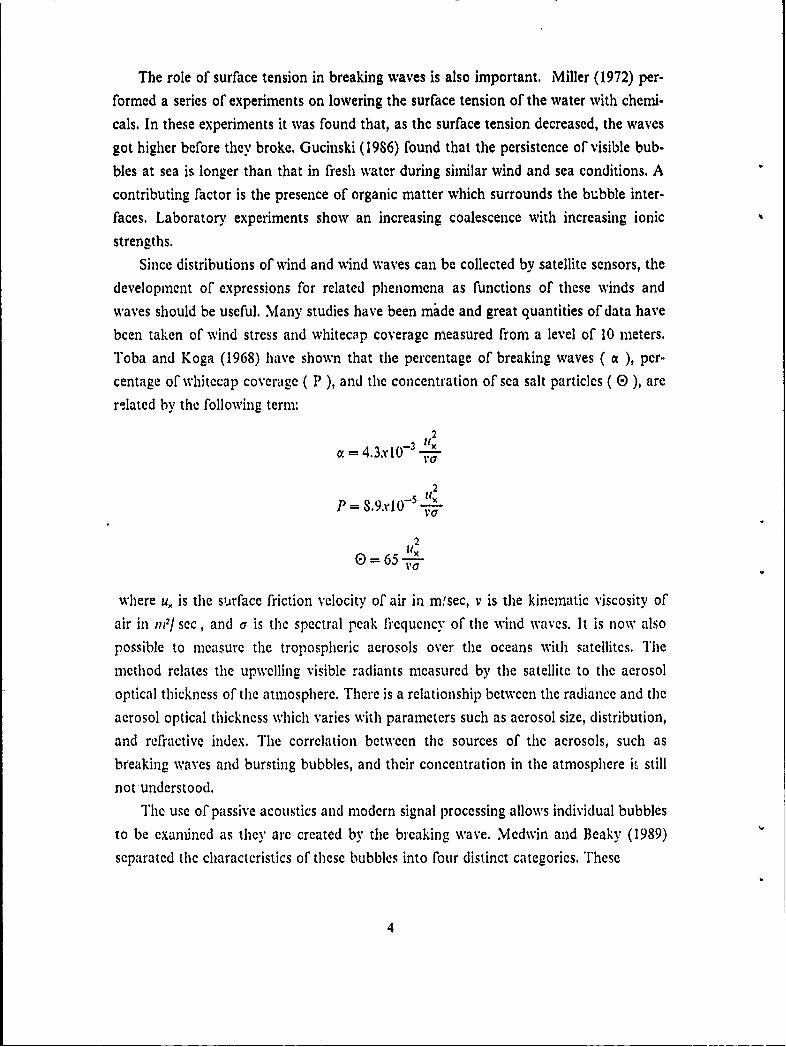
The role of surface tension in breaking waves is also important. Miller (1972) per-

formed a series of experiments on lowering the surface tension of the water with chemi-

cals. In these experiments it was found that, as the surface tension decreased, the waves

got higher before they broke. Gucinski (19S6) found that the persistence of visible bub-

bles at sea is longer than that in fresh water during similar wind and sea conditions. A

contributing factor is the presence of organic matter which surrounds the bubble inter-

faces. Laboratory experiments show an increasing coalescence with increasing ionic

strengths.

Since distributions of wind and wind waves can be collected by satellite sensors, the

development of expressions for related phenomena as functions of these winds and

waves should be useful. Many studies have been made and great quantities of data have

been taken of wind stress and whitecap coverage measured from a level of 10 meters.

Toba and Koga (1968) have shown that the percentage of breaking waves ( a ), per-

centage of whitecap coverage ( P ), and the concentration of sea salt particles ( E ), are

rmlated by the following term:

2

a =4.3x10 - xA

VC2

P = S.9X05 X

2

where ux is the surface friction velocity of air in m/sec, v is the kinematic viscosity of

air in nil/ sec, and a is the spectral peak frequcncy of the wind waves. It is now also

possible to measure the tropospheric aerosols over the oceans with satellites. The

method relates the upwelling visible radiants measured by the satellite to the aerosol

optical thickness of the atmosphere. There is a relationship between the radiance and the

aerosol optical thickness which varies with parameters such as aerosol size, distribution,

and refractive index. The correlation between the sources of the aerosols, such as

breaking waves and bursting bubbles, and their concentration in the atmosphere iL still

not-understood.The use of passive acoustics and modern signal processing allows individual bubbles

to be exanined as they are created by the breaking wave. Medwin and Beaky (1989)separated the characteristics of these bubbles into four distinct categories. These

4

categories describe the bubble damping, resonance frequency, and oscillation patterns.

With the method described in this thesis, utilizing the same equipment as Medwin and

Beaky, the location of these individual bubbles can be determined from the geometry ofthe hydrophone array and the difference in the time of arrival of the pressure field to theindividual elements. From this data the exponentially decreasing temporal rate of bubblecreation from an individual breaking wave can be calculated, as well as the productiondensity in bubbles per unit area originating from a single breaking wave. The volumeof gas encapsulation per unit surface area of a spilling breaker can be computed from

the bubble density. This could be useful in studies of gas exchange at the ocean surface.

If all the information and methods described can be integrated and successfully uti-lized it will be possible to obtain a complete perspective on the generation of bubblesat sea. The background bubbles are understood and can be measured; the main sourceof bubble creation, particularly whitecap coverage from breaking waves, can be esti-n: ited; the physical and chenical makeup o1 the water can be examined; and now with

the use of the method described in this thesis it is possible to predict the rate of bubbleproduction f'rom the whitecaps. This information, when combined, will flurther aid in our

understanding the effect of air'sea interaction on our environment.

111. FACILITIES AND APPARATUS

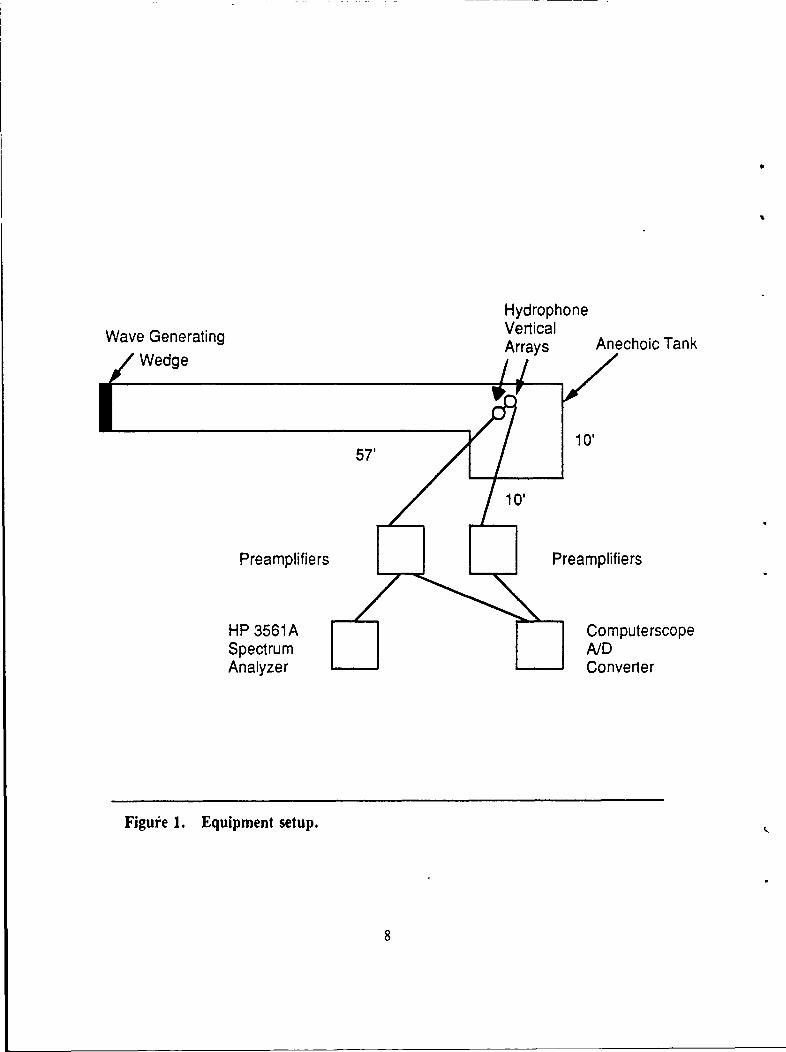
The laboratory facilities include a 57x4x4 foot wave tunnel emptying into a10xl0xl0 foot anechoic tank, A motor-driven reciprocating wedge generates the wavesat the beginning of the tunnel. The waves break approximately three feet after enteringthe tank. The exact positiorn of where the waves will break was not controlled. The tank

sides and bottoms are lined-with Redwood pilings. After spilling, the waves are absorbed

by a "beach" consisting of an aluminum shavings wedge which minimizes the wave re-flection at the tank boundary.

Medwin and Beaky (1989) conducted tests in the tank which demonstrated at leasta 15 decibel diff'erence between a signal and the strongest reflection from the tank walls

at frequencies under 5 kl-z, and at least 20 dB at frequencies above 5 kllz, when thehydrophone is 24 cm from the bubbie source. The signal to reverberant noise ratio isbetter for shallower hydrophones.

Two vertical arrays of 2 oniidirectional hydrophones with the shallow hydrophoneat a depth of 15 cm and the deep hydrophone at a depth of 31 cm are situated in theapproximate area where the majority of the waves break as depicted in figure (1). The

output signals are input into an Ithaco 1250 voltage amplifierbandpass filter with thebandpass frequencies set between 300 liz and 100 kHz. The amplifier output splits into

a Hewlett-Packard 3561A signal analyzer and also into an IBM XT personal computerwith an R. C. Electronics "computcrscope" analog to digital converter. The signal ana-lyzer and the "computerscope" allow the operator to select triggering level. The signalanalyzer triggers at an input level of 0.837 Volts which, for an amplification of 5000,

corresponds to an acoustic pressure of 1.4 Pascals.

This "computerscope" analog to digial conversion software package samples thedata with a sampling period of 1 microsecond with one input, 2 nicroseconds with two

inputs, and accordingly, -; microseconds with four inputs with a 12 bit amplitude resol-ution. The sampled signal is displayed both graphically and numerically with cursermovement. The buffer is 64 milliseconds long with the minimum sampling period of 1microsecond and can be lengthened by a corresponding increase in the ,ampling period.

Sections of the buffer can be "expanded" or "compressed" in time and the amplitude of

6

the signal display can also be adjusted. This enables the user to manipulate the-graphical

presentation to obtain a signal that can be accurately analyzed and also to adjust the

sampling rate to maximize the signal resolution.

Hydrophone

Wave Generating Vertical

Wedge Arrays Anechoic Tank

57' 10

10'

Preamplifiers Preamplifiers

HP 3561A ComputerscopeSpectrum A/DAnalyzer Converter

Figure 1. Equipment setup.

IV. EXPERIMENT

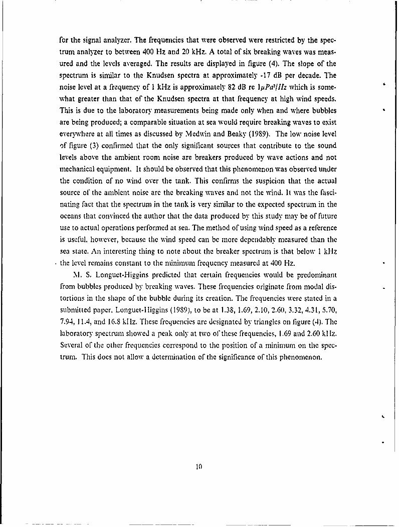
A. BREAKER SPECTRUMDuring World War I I many observations of the ambient noise of the oceans showed

that "wind noise" is the primary source of the noise in the frequency range between 500

Hz and 20 kHz. The famous Knudsen spectra broke down this large collection of data

in a manner intended to demonstrate the wind speed dependence of the noise level. This

spectrum is reproduced from Urick (1983) as figure (2). The possible processes, as given

by Urick, which produced this noise were hypothesized to be "crash noises of breaking

waves", "flow noise" produced by wind moving over the water, "cavitation noise", and"wave generating actions" of the wind. The paper by Medwin and Beaky (1989) proves

that the catastrophically created, damped bubbles, by themsclves, explain the Knudsen

spectra. The slope of the noise spectrum in this frequency band is approximately -5 to-6 dB per octave or -17 dB per decade with the level increasing with wind speed. The

noise in the frequencies outside this band was believed by Urick to originate from

sources not directly dependant on wind speed such as shipping below 500 Hz and ther-

nial noise above 50 kHz.

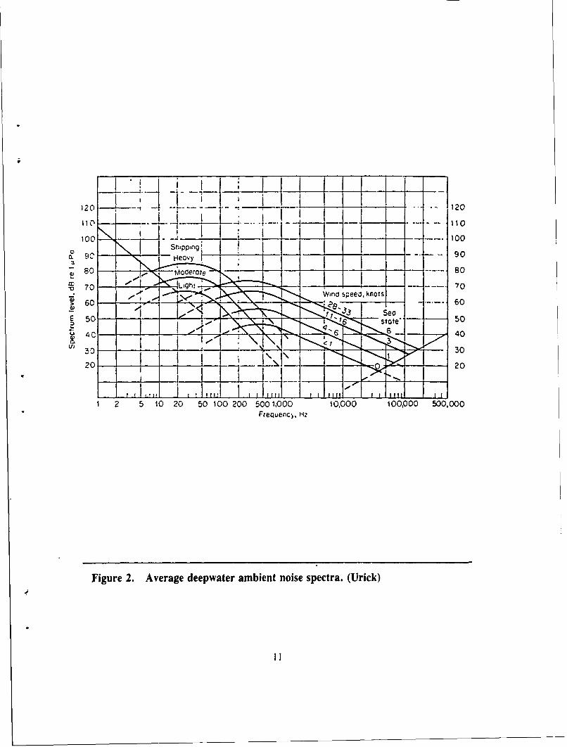
In order to deternine the noise spectrum of the waves breaking in the tank it was

first necessary to ensure that the wave generating equipment was not acting as an addi-

tional noise source. Figure (3) shows the background ambient noise of the tank with no

equipment in operation plotted with a dashed line. The ambient noise in the tank with

the plunger in operation but no waves breaking is plotted with a solid line. Both plots

were gcneratcd on the liP 3561A spectrum analyzer using a time average of 300 input

signals, each of 500 milliseconds duration. The signal level was computed For frequencies

between 500 Hz and 50 kI-Iz.

The breaker spectrum was also obtained using the I IP 3561A with the input from

an onmidirectional hydrophone at a depth of 24 cm. The signal was divided into 40 se-

quential records, each of 20 millisecond duration. Each 20 millisecond band was Fourier

transformed to provide the power for each 50 Hz block of the buffer.'4 The energy in

these bands was summed only if the energy was 3 dB above the noted ambient noise level

of the tank with no activity. This was done to ensure that the energy originated only

from breaking waves in the tank. The breaking of a wave can usually be identified by

a relatively high amplitude low frequency bubble which served as the triggering source

9

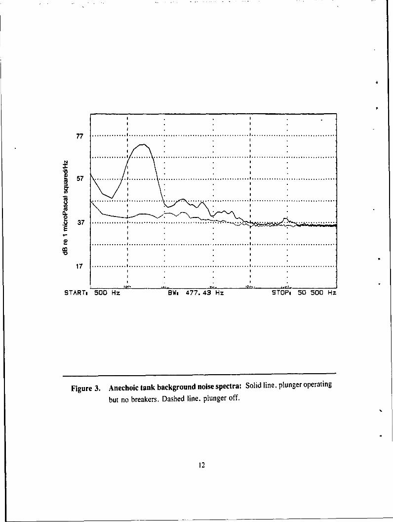
for the signal analyzer. The frequencies that were observed were restricted by the spec-trum analyzer to between 400 Hz and 20 kHz. A total of six breaking waves was meas-

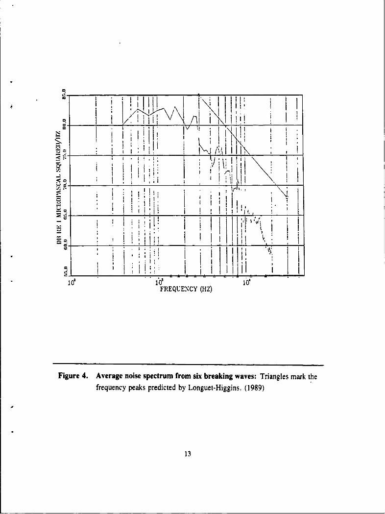
ured and the levels averaged. The results are displayed in figure (4). The slope of the

spectrum is similar to the Knudsen spectra at approximately .17 dB per decade. Thenoise level at a frequency of I kHz is approximately 82 dB re IPa/Ilz which is some-what greater than that of the Knudsen spectra at that frequency at high wind speeds.

This is due to the laboratory measurements being made only when and where bubblesare being produced; a comparable situation at sea would require breaking waves to exist

everywhere at all times as discussed by Medwin and Beaky (1989). The low noise level

of figure (3) confirmed that the only significant sources that contribute to the soundlevels above the ambient room noise are breakers produced by wave actions and not

mechanical equipment. It should be observed that this phenomenon was observed underthe condition of no wind over the tank. This confirms the suspicion that the actual

source of the ambient noise are the breaking waves and not the wind. It was the fasci-

nating fact that the spectrum in the tank is very similar to the expected spectrum in the

oceans that convinced the author that the data produced by this study may be of futureuse to actual operations performed at sea. The method of using wind speed as a reference

is useful, however, because the wind speed can be more dependably measured than thesea state. An interesting thing to note about the breaker spectrum is that below I kHz

the level remains constant to the minimum frequency measured at 400 -Iz.

M. S. Longuet-Higgins predicted that certain frequencies would be predominantfrom bubbles produced by breaking waves. These fi'equencies originate from modal dis-

tortions in the shape of the bubble during its creation. The frequencies were stated in asubmitted paper. Longuet-Iliggins (1989), to be at 1.38, 1.69, 2.10, 2.60, 3.32, 4.31, 5.70,

7.94, 11.4, and 16.8 kl Iz. These frequencies are designated by triangles on figure (4). The

laboratory spectrum showed a peak only at two of these frequencies, 1.69 and 2.60 kl Iz.

Several of the other frequencies correspond to the position of a minimum on the spec-

trum. This does not allow a deternination of the significance of this phenomenon.

10

12012

100 S.100

& 0 - - - --- . 90

80 - -oeoej~80

70-* ,- Ligh? . 7 0

2 ~6 stote"5

20 20

1 2 5 10 20 50 100 200 500 1,00 10,000 100,000 500,000Frequency, HZ

Figure 2. Average deepwater ambient noise spectra. (Urick)

7 7 . ... ... ... .. . . . ... . . . . . . . . .. . . . . . ... .. . . . . . . . .. . . . . . . .

.. .. .. . . . . . . ... . . . . . . .. . . . . . .. .. . . . . . . . .. . . . . . . .

57 .. .. .. . . .. .. .. . .. . . . . . . . . . . . . . ... .. . . . . . . . .. . . . . . . .

........ .

....

E . .....

17 .. . . . . . . . . . . . . . . . .. . . . . . .. . . . . . .. . . . . . . . . .

STR~ 57 zB 77-3zSO 050H

but no bekr. Dahdln.pugrof

c12

+I I' 'lIII l I I" ' " I' IIIII

id' i 'd;

=I 1 V 1 !1 ' i i +____ I ____1 !+ ''4______

" ___ __ _ I i_ ___ __ ' i i i l f i j! _'____ I

i I " I

F r. , oI s' ,o , brekI I iI.m t

II' I I ' 'i'- ,t If

* : ,hi ! ! .;,!.--.:i , ii Ii ,,

= i 'i i" !,I ' ' 1W '• I I " .

',, ,- i _____ i ! I il i ' I "" ' !

frequency peaks predicted by Longuet-Higgins. (1989)

13

B. BUBBLE IDENTIFICATION

It is possible to positively identify individual bubbles within the sound originating

from the breaking of a wave. The equipment utilized is a hydrophone, a preamplifier,

and an IBM XT personal computer with an R.C. Electronics Computerscope analog todigital converter. The converter samples the signal and allows detailed viewing of the

desired segments of the captured noise.

When a wave breaks or "spills" air is entrained, bubbles are formed, and t. le bubbles

oscillate to become sources of noise. In every wave observed with the signal processing

equipment, the moment when the wave breaks can be identified by a large amplitude,

low frequency bubble, with suflicient energy to be used as the triggering source for the

signal analyzing equipment.

This equipment has already been used by Medwin and Beaky (1989) to characterize

the bubbles from breaking waves by identifying the damping and modulation aspects

most commonly observed. Four distinct oubble scenarios were classified: spherical bub-

bles with either a constant decay rate or with two different decay rates, a damped oscil-

lation bubble appearing to shed a-much smaller bubble, a near surface bubble which has

an increasing amplitude as it moves away from the surface due to an increase in the

dipole axis, and a bubble undergoing amplitude modulation possibly due to another

bubble in close proximity with a slightly different frequency.

The resonance frequency of the bubbles was converted to bubble radius using the

following relationship from Clay and Medwin (1977):

1 3 )PI

where f is the resonance frequency of the bubble in Hz, a is the bubble radius in meters,

y is the ratio of specific heats of the gas in the bubble, P is the hydrostatic pressure in

Ni'/i, and p is the density of the water in kg/in:3

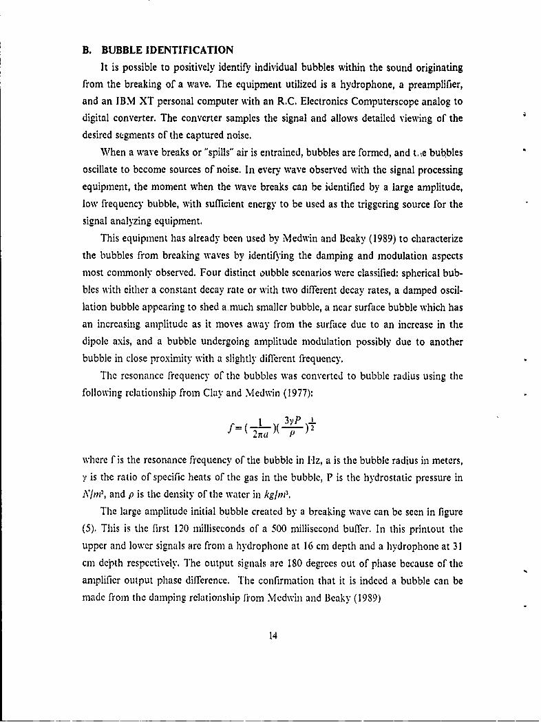
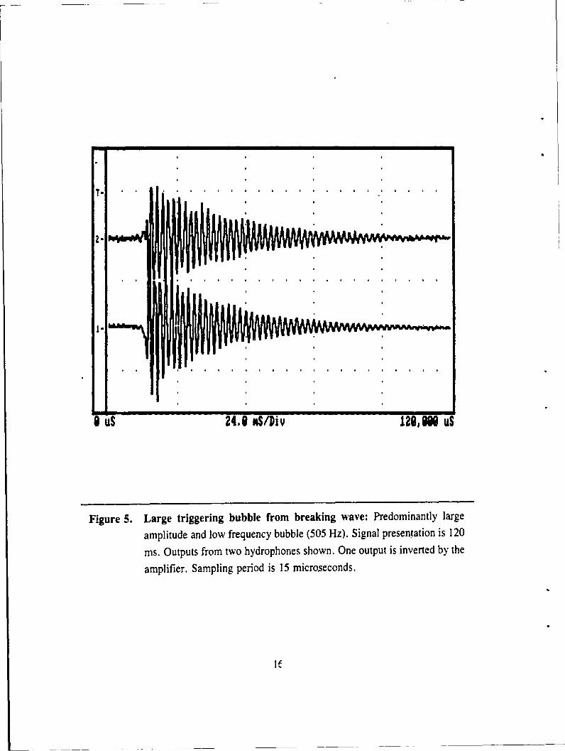
The large amplitude initial bubble created by a breaking wave can be seen in figure

(5). This is the first 120 milliseconds of a 500 millisecond buffer. In this printout the

upper and lower signals are from a hydrophone at 16 cm depth and a hydrophone at 31

cm delith respectively. The output signals are 180 degrees out of phase because of the

amplifier output phase difference. The confirmation that it is indeed a bubble can be

made from the damping relationship Iiom Medwin and Beaky (1989)

14

1Tf

where r is the decay time in seconds to 1,e of its amplitude, f is the resonance frequency

in Hertz, and 6 is the damping constant. The measured frequency of the bubble in figure(5) is 505 Hz and the measured 11e decay time is 30.9 milliseconds. From the table onpage 199 of Clay and Medwin (1977) the damping constant for this frequency should

be approximately 0.022. If placed in the above equation this damping constant yields a

1;e decay time of 28.6 milliseconds, a difference from the measured value of 7 percent.This is close enough to the theoretical value to ascertain that the bubbles are behaving

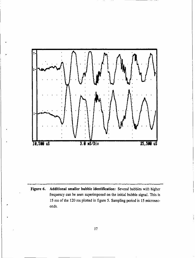
as expected. If the presentation is expanded and viewed with more detail as in figure (6),additional later signals from higher frequency, smaller amplitude bubbles can be seen

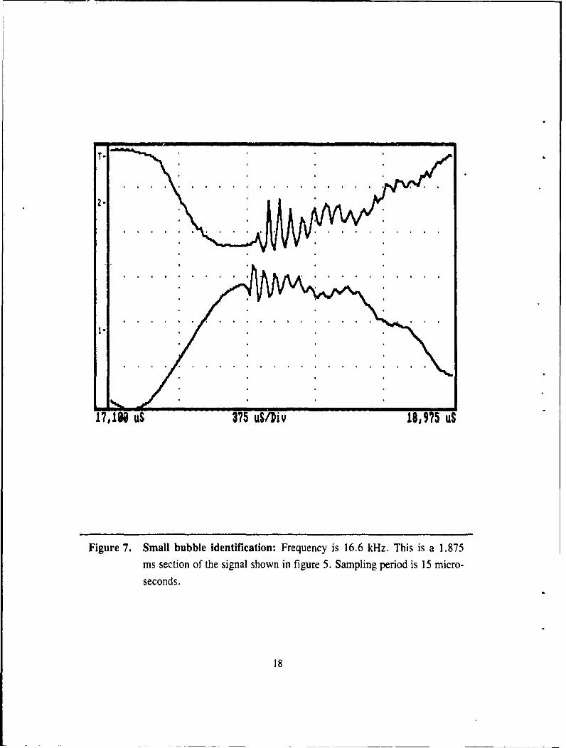
superimposed on the low frequency bubble signal. Finally, the presentation can be ex-panded even further, figure (7), to enable the accurate identification of a smaller bubblewith frequency 16.6 kHz (196 micron radius) and accurate measurement of tile difference

in time of arrival of the signal to the individual hydrophones.It can be seen in the above figures that the individual bubbles call be identified with

enough resolution to obtain accurate information about bubble frequency, amplitude,

and relative time of arrival at the hydrophones. The signal data was recorded only if abubble could be confidently identified above any noise which may have been received.With this equipment accurate identification could be ensured if the signal level was atleast 3 decibels above the measured ambient noise level of 37 dB re lPPa21/lz at the

hydrophones. The resulting bubble count is thereby a conservative measure of thenumber of bubbles and would not include any bubbles with received signal less than the

linit of 37 dB.

15

I us 24.6 ftS/Di Y 129, onus

Figure 5. Large triggering bubble from breaking wave: Predominantly large

amplitude and low frequency bubble (505 Hz). Signal presentation is 120

ns. Outputs from two hydrophones shown. One output is inverted by the

amplifier. Sampling period is 15 microseconds.

T-

1-

M-05N uS 3.9 NS/Diy 25,5W uS

Figure 6. Additional smaller bubble identification: Several bubbles with higher

frequency can be seen superimposed on the initial bubble signal. This is

15 ms of the 120 ms plotted in figure 5. Sampling period is 15 microsec-onds.

17

-

. . . . . .. ..

1-

17,18 uS 375 uS/Div 18,95 us

Figure 7. Small bubble identification: Frequency is 16.6 kHz. This is a 1.875ms section of the signal shown in figure 5. Sampling period is 15 micro-seconds.

18

C. BUBBLE LOCATION

The location of the bubble can be deternined using the geometry of the hydrophone

positions and the relationships developed from the difference in time of arrival of the

sound pressure wave to the hydrophones. In this procedure it was assumed that the

bubbles were created and remain approximately at the surface of the water. The argu-

ment for this assumption follows: the bubbles were produced from the action of the

breaking wave entraining pockets of air. This catastrophic force was the driving mech-

anism causing the oscillation. It was observed that the bubble oscillations only lasted for

a short duration, of the order of tens of milliseconds, after the bubble formation. In this

short period of action the bubble could not physically travel any significant distance.

A second assumption is that the surface of the water remained horizontal, ignoring

the wave height. The error due to this assumption will be examined shortly.

When two hydrophones are placed in a vertical array the sound pressure wave from

a bubble at the surface will arrive at the hydrophones at diflerent times. This difference

in time of arrival will be a function of the distance the wave must travel through the

water.

Bubbles produced near the surface of the water act as dipole sources. The dipole

consists of the bubble and an imaginary source the same distance above the surface as

the bubble is below, with a distance L separating this image and the bubble. With the

assumption that kL < I, the dipole radiation pattern will be defined by the following

equation from Morse and Ingard (1968):

_ k2 .. .,tw -t

P /2 )pcD cos(0)(1 + kR )e!(wkR)

where k is the wave number in radians:meter, R is the range in meters from the bubble

to the hydrophone, pc is the acoustic impedance of water in Pa sec:m, D = VL where

V = 4na2U is the volume per time, U is the radial velocity amplitude, 0 is the angle be-

tween the axis of the dipole and the line adjoining the bubble and the hydrophone, and

w is the angular frequency of the oscillating bubble in radians,'second. The magnitude

of the pressure at hydrophone 1 can be described as

i I =[k2 pcD cos(-4 - )][I + 1

Using the relationship

19

2 2--fto

a+ib-(a +b2e

so that the term

+ + 2 -eokR'' k

and

0 - tan-'(bL 1= tan-'(k 1

The real part of the pressure at hydrophone 1 can now be described by the equation:

P, = I P3 I Re(e (%"'- kRI +0))

or restated

P = I P I cos(wtl - kRI + tan-,( )

Identically, the real part of the pressure at hydrophone 2 can be written:

P2 = I P2 1 cos(w 2 - kR2 + tan'(I)).

Comparing the phases for the times that the peaks occur,

wt- kR I + tan-I( -)=nnwt I I

and

i 2 - kR 2 + tan-'( 1) =nnWkR2

and subtracting yields:I 1

1412 - tj) - k(R2 - RI) + tan-( -- ) - tan-( - 0.R2 kRI

The equation describing the difference in time of arrival can be written as:

20

t2-t ,c R, + (-"L7) tan-'( )-( )tan-'( )22 )R 3 2irf LX2

where R, and R, are the distances from the bubble to the hydrophones in meters, k is the

wave number in radiansmeter, c is the speed of sound in meters'second, and f is the

resonance frequency of the bubble in Hertz.

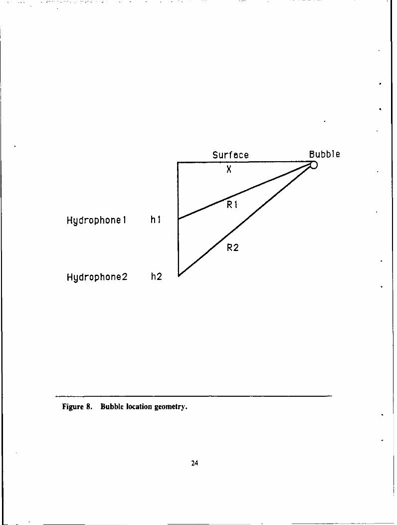
The geometry of the hydrophones is depicted in figure (8). The following relation-

ships should be noted:

R, (=h + x2)22 2 1

R2 =0 + x F2

where h, and h2 arc the depths of the hydrophones in meters and x is the horizontal dis-

tance on the surface of the water above the hydrophone array in meters. If the position

on the surface above the hydrophones is treated as an origin, x is in fact the radius of acircle. If these equations for R, and R2 are placed in the previous equation for time of

arrival difference, this radius, x, will remain the only unknown. Using an iterative pro-

gram, the computer will easily determine the solution.

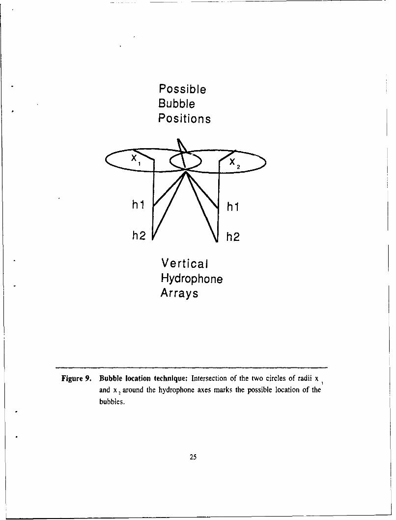
The position of the bubble on the surface can be determined by using two verticalarrays of hydrophones. The bubble will be located somewhere on the circles surrounding

the arrays. These circles will intersect at two points, in a symmetrical manner about the

horizontal line separating the arrays as in figure (9). The ambiguity between the two

intersections is unimportant to the objectives of the experiment.

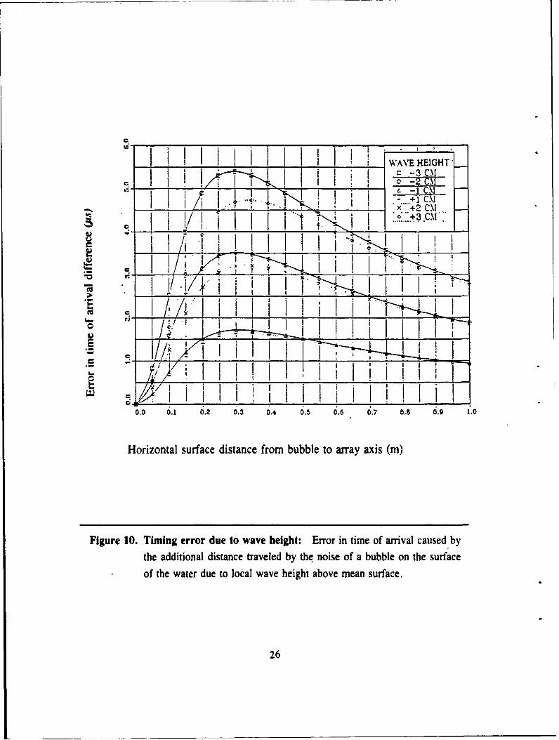
The fact that the surface of the water is not constantly horizontal, but in reality

consists of various wave heights, causes a change in the time of arrival difference be-

tween the hydrophones of an array. If the bubble is located on a wave crest or trough

the distance the pressure wave will have to travel can be described by:

2) 2!Ri = (( 1 +Ah), +x) 2

R2 = ((h2 + Ah) 2 + x2)T

where Ali is the vertical difference in bubble position from the horizontal surflace of thewater. This difference in time of arrival caused by the wave amplitude is shown in figure

(10). It will be noted that the maximum amplitude of the waves in the tank is

21

approximately 3 cm. At this wave height the error in time of arrival is only 5 microsec-

onds. Because of the fact that the wave height follows a Gaussian distribution, the wave

height at the bubble location will likely be on the order of 1 cm and the error in time

would be 2 microseconds with a corresponding error in bubble location of an insignif-

icant 2 or 3 millimeters.

Two vertical arrays, each including a shallow hydrophone at 16 cm depth, and a

deep hydrophone at 31 cm depth, were placed in the tank in the area where most waves

break. The perpendicular line between the hydrophone arrays was set at approximately

a 30 degree angle to the direction of the wave propogation in order to ensure geometric

efficiency in the calculation of bubble positions. The buffer length was set to 100 milli-

seconds with a corresponding sampling period of 6 microseconds (spatial resolution, 9

mnm). This small sampling period was considered necessary in order to measure the time

of arrival difference as accurately as possible. The output went through the preamplifiers

set at a gain of 5000 and acted as the trigger to the computerscope analog to digital

converter.

The difference in time of arrival to the two vertical pairs of hydrophones, the reso-

nance frequency of the bubble, and the time that the bubble began oscillating relative

to the breaking of the wave, were recorded in the first 100 milliseconds for each bubble

created by a breaking wave. This information was used with the iterative computer

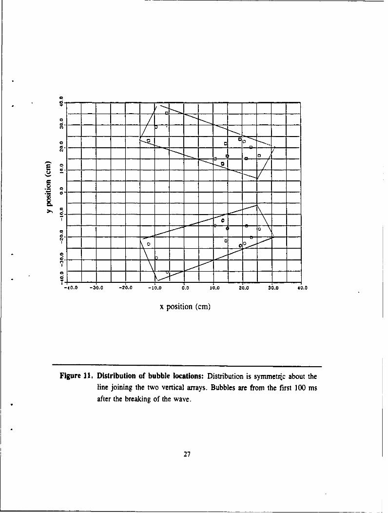
program to plot the locations of the individual bubbles. Figure (11) is the result of one

breaking wave showing the symmetrical distribution of the bubbles created in the first

100 milliseconds after breaking. The symmetrical locations are caused by the two inter-

sections of the bubble radii circles about the axes of the hydrophones. As long as the

wave does not break close to the hydrophones it is not necessary to plot both sets of

location positions because it is the relative positions of the bubbles that is necessary for

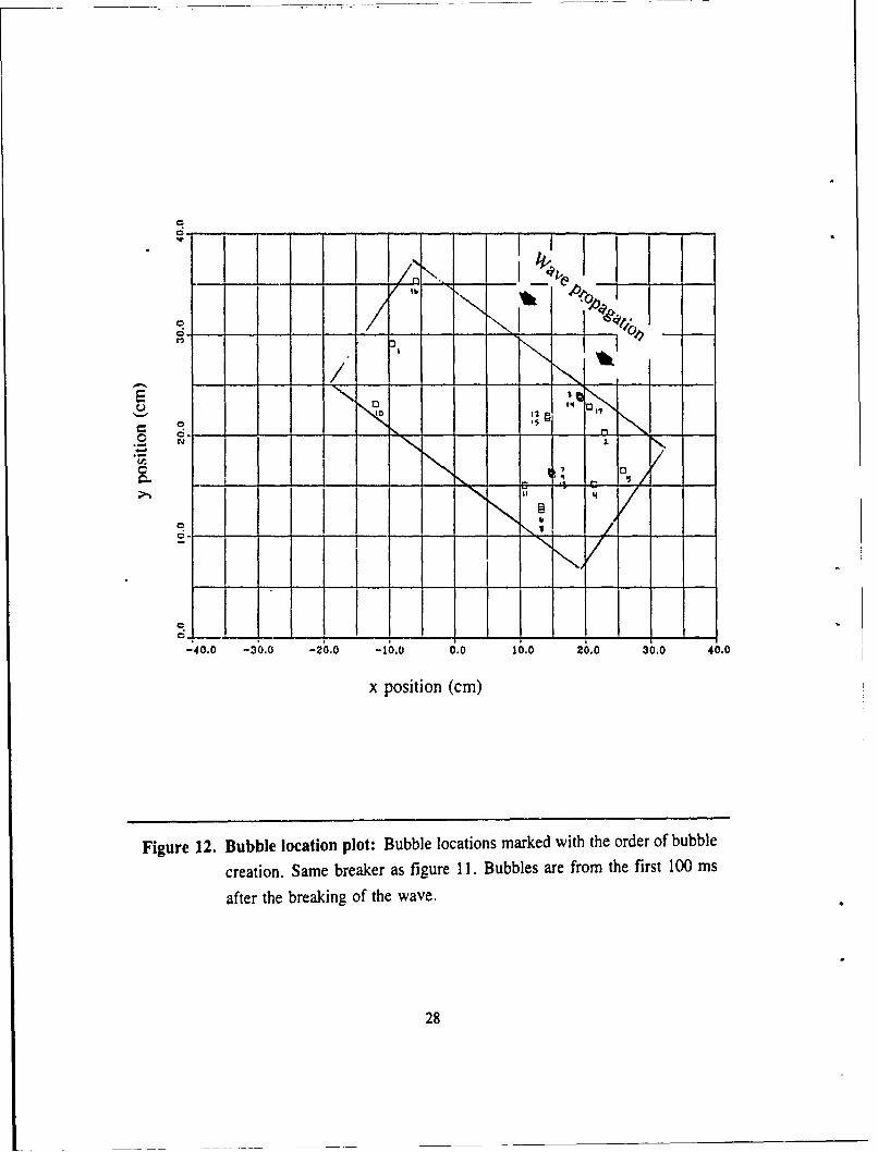
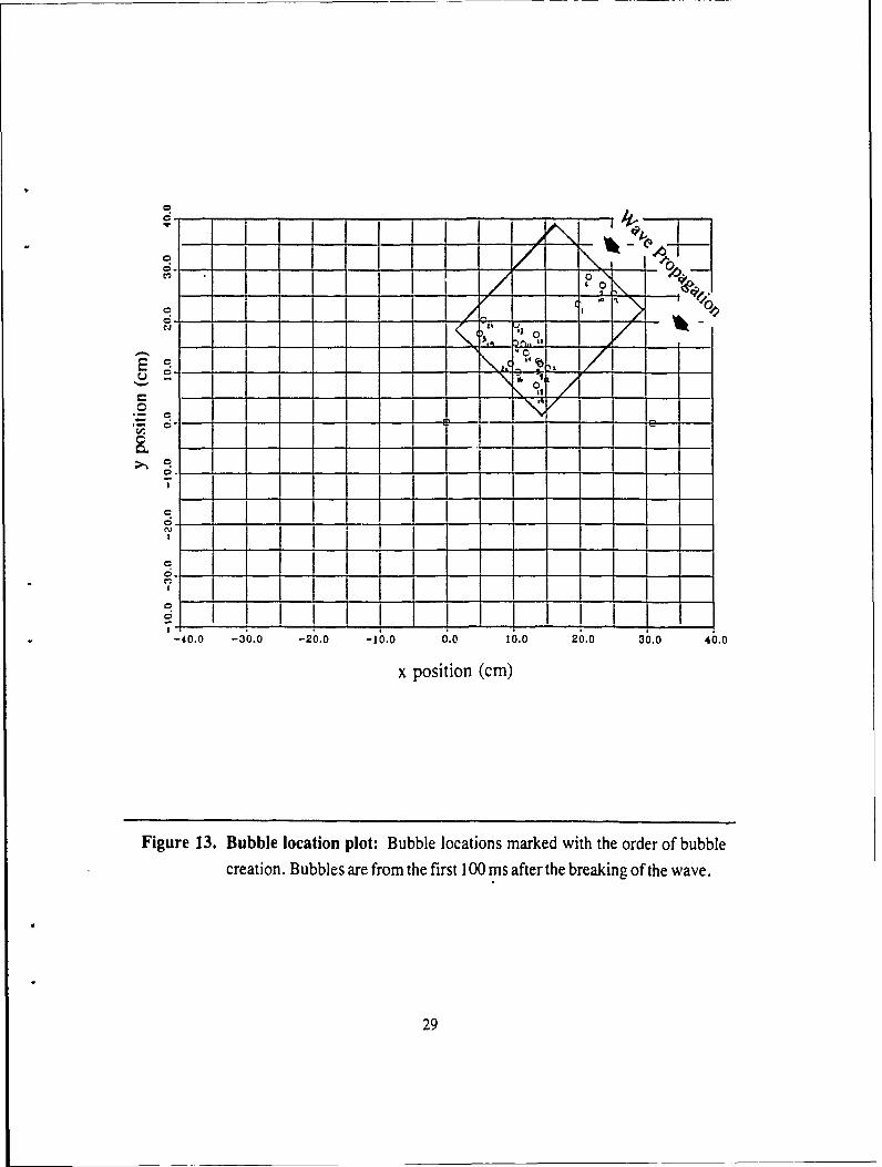
density calculations. Figures (12) and (13) show the bubble locations with only the pos-

itive positions recorded.

The position plots demonstrate the bubble patches or "hot spots" often noted in

acoustical measurements at sea. The plots were divided by a grid consisting of squares

5 cm on a side. These blocks of 25 square centimeters were used to calculate the area

over which bubbles were produced. This large area assigned to any bubble counters and

compensates for any error in the calculation of bubble position. Each square with a

bubble in residence was counted. The average total area of bubble production was 345

square centimeters per breaking wave with a standard deviation of 42 square centime-

ters. It was assumed that all bubbles created by a breaker originate in such a calculated

22

area. It was not possible to expand the time of observation in order to confirm this as-

sumption for later bubbles because the sampling period would also have become longer

and the resolution of the time of arrival difference would not have been sufficient for

accurate bubble location. Another method was to form a rectangle around the bubbles

and compute the production area. The average production area calculated with this

method was 320 square centimeters with a standard deviation of 96 square centimeters.

The rectangle is marked by a solid line around the bubbles in figures (12) and (13). The

two methods compare within 10 percent for the average production areas.

Another result of the bubble position plots was the ability to label the order in which

the bubbles were created by the breaking wave. Figures (12) and (13) also show these

relative positions of the bubbles from two waves each marked with the order in which

they were produced. The order of the positions does not demonstrate that the location

of the bubble depends on the relative time of its creation with respect to the breaking

of the wave. The first bubble created was not necessarily the closest to the positionwhere the wave breaks, Also the last bubble created was not necessarily located the far-

thest along the direction of wave propagation from the position where the wave began

breaking. This fact suggests that the majority of the bubbles created were located within

the area calculated even though this area was calculated from bubbles originating in the

first 100 nlliseconds of breaking.

Bubbles observed within the bubble location plots were ocassionally positioned in

roughly linear patterns not necessarily perpendicular to the direction of wave

propogation. The bubbles within these patterns all originate consecutively in short

widows of time. It is believed that these bubbles are created by and along the small

capillary waves which sometimcs are seen superimposed on the face of a main wave. This

evidence of capillary waves is examincd in Appendix A.

23

Surface Bubblex

Ri

Hydrophonel hi

R2

Hydrophone2 h2

Figure 8. Bubble location- geometry.

24

PossibleBubblePositions

x x2

h1 2

hi hi

h2 h2

VerticalHydrophoneArrays

Figure 9. Bubble location technique: Intersection of the two circles of radii xand x around the hydrophone axes marks the possible location of the

bubbles.

25

_____ __ WAVE HEIGHT'I I ' ______

I t !rT .4r ___II_ -axi1 I:/T I i I I : I II _-c _

, 1 , o' #-i -i -. i-I' - cM -

I c I - CI- '...1 c

J " -iI I'I " : - -!

"/ / _ __ , I ! _L __ i ' ,-l

0.0 0.1 0.2 0.3 0.4 0.5 0.6 0.7 0.B o.9 1.0

Horizontal surface distance from bubble to array axis (in)

Figure 10. Timing error due to wave height: Error in time of arrival caused by

the additional distance traveled by the noise of a bubble on the surface

of the water due to local wave height above mean surface.

26

E

-0.0. - -20.0 -10.0 0. 100 2. 00 4.

,. - - - ,.- .. - g = .N

-00 - .0 00-100 - |. - 0.0 $ 0 - 0.

x position (cm)

Figure 11. Distribution of bubble locations: Distribution is symmetric about theline joining the two vertical arrays. Bubbles are from the first 100 msafter the breaking of the wave.

27

00"

C

o -,

- -- ,I \ /

o0 , , ..

>11

0J

-4 .0 -3 .0 - .0 - 1.0 .0 1 .0 2 .0 30.0 ,4o.0

x position (cm)

Figure 12. Bubble location plot: Bubble locations marked with the order of bubble

creation. Same breaker as figure 11. Bubbles are from the first 100 ms

after the breaking of the wave.

28

000.~ *

0 %

o I: t

; io

-40.0 -3 0. 0 -2 6 -1 0. 0 6.0 1 . . 0 30.0 4 0. 0

x position (cm)

Figure 13. Bubble location plot: Bubble locations marked with the order of bubble

creation. Bubbles are from the first 100 ms after the breaking of the wave.

29

D. RATE OF BUBBLE PRODUCTION

It was observed from the use of the Hewlett-Packard 3561A Spectrum Analyzer that

noise is produced from a breaking wave for a period of 2 to 3 seconds after the first

sound of a breaking wave is heard. The digital processing equipment used to identify,

locate, and count bubbles hr ; a relatively small memory (64k bites). This does not per-

mit the sound to be captured for a long enough period of time to record all bubbles

produced and simultaneously have a sampling period small enogh to be of use in the

identification of bubble resonance frequencies. Therefore it was thus necessary to deter-

mine the rate at which bubbles are produced over time in order to determine an ex-

pression defining the bubble production rate relative to the time at which the wave

breaks. The measurements could then be made for shorter periods of time and then ex-

trapolated to determine the total number of bubbles produced.

Two orrmnidirectional hydrophones were placed in a vertical array in the tank at

depths of 12 and 24 centimeters. The buffer length for two hydrophoncs was expanded

to 500 milliseconds by using a sampling period of 15 microseconds. Through exper-

imentation and consideration of the Nyquist relationship it was deternined that this was

the maximum sampling period that would allow dependable identification of bubbles

with resonance frequencies less than 33 kllz. The trigger level was adjusted to a level

sufficiently high to ensure the sampling equipment would begin capture only when a

wave was breaking almost directly above the hydrophones. This was done to guarantee

the observation of bubbles with a small amplitude which may not have been seen from

a longer distance and at a greater angle from the dipole. The short range from the

hydrophones can be confirmed using the method previously described. The input signal

passed through the preamplifier with the gain set on 5000. A total of 10 breaking waves

were observed.

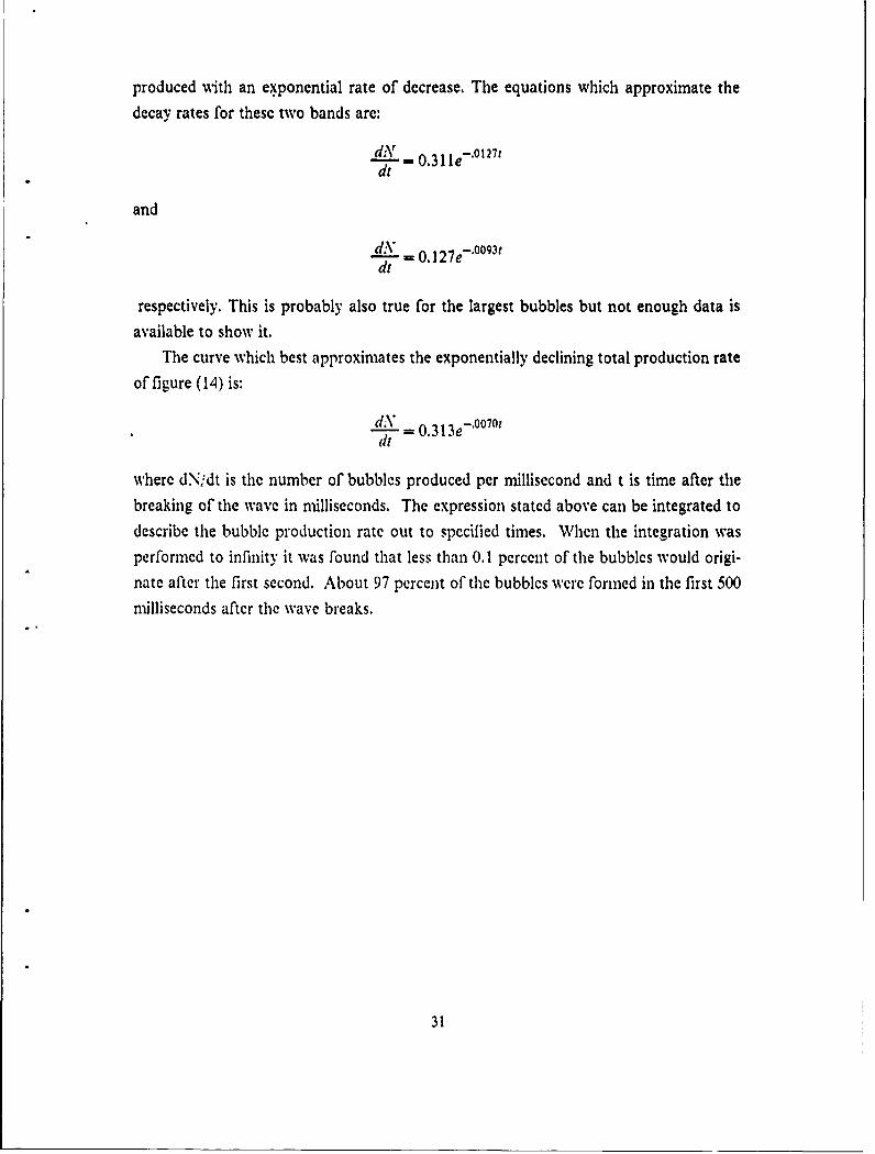
The average number of bubbles of all radii produced per breaker, within time incre-

ments of 10 milliseconds, is plotted against the time after the breaking of the wave in

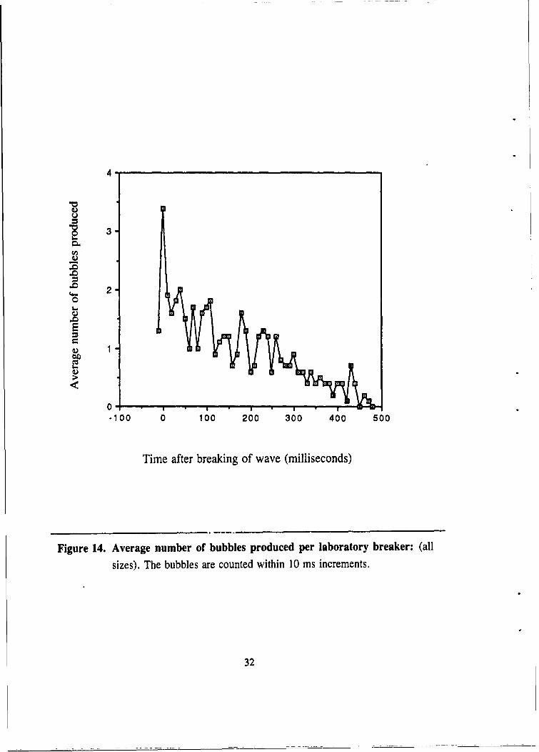
figure (14). Additionally, the production rates for bubbles with bubble radii broken down

into bands of greater than 2.2 mm (resonance frequency less than 1500 Hz), between 2.2

mmn (1500 Hz) and 0.16 nm (20 kHz), and less than 0.16 nm (greater than 20 kHz), are

depicted in figures (15), (16), and (17) respectively. These bands are chosen to accentuate

the bubble production behavior in the Knudsen sea noise spectrum frequency regime

generally taken to be between 500 Hz and 20 kHz.

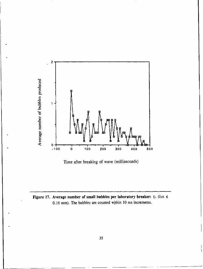
The production spectrum of the two radii bands, 0.16 to 2.2 nm and smaller than

0.16 mm as seen in figures (16) and (17), suggests that bubbles in these bands are

30

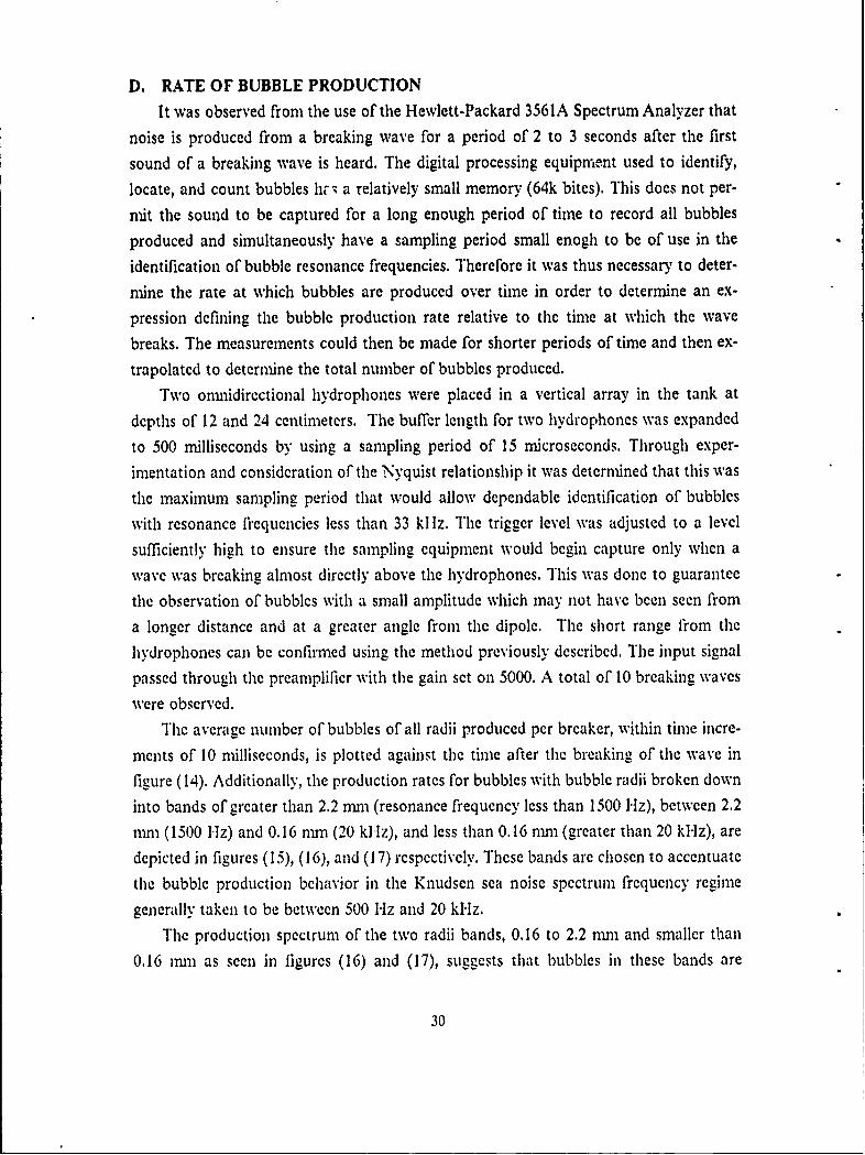
produced with an exponential rate of decrease. The equations which approximate the

decay rates for these two bands are:

dN 0.31 le 27

and

dV = 0.127e -' 0093t

dt

respectively. This is probably also true for the largest bubbles but not enough data is

available to show it.The curve which best approximates the exponentially declining total production rate

of figure (14) is:

d = - 0.313e -0° °7°'It

where dN:dt is the number of bubbles produced per millisecond and t is time after thebreaking of the wave in milliseconds. The expression stated above can be integrated to

describe the bubble production rate out to specified times. When the integration wasperformed to infinity it was found that less than 0.1 pcrcent of the bubbles would origi-

nate after the first second. About 97 percent of the bubbles were formed in the first 500milliseconds after the wave breaks.

31

4-

2-

E1

0 1

-100 0 100 200 300 400 500

Time after breaking of wave (milliseconds)

Figure 14. Average number of bubbles produced per laboratory breaker: (all

sizes). The bubbles are counted within 10 ms increments.

32

,5

< .4

3.3.

EC)

C.)

< 0'

-100 0 100 200 300 400 500

Time after breaking of wave (milliseconds)

Figure 15. Average number of large bubbles per laboratory breakq*: (radius2.2 mm). The bubbles are counted within 10 ms increments.

33

2

E.

1 1

.10 0o 100o 200 300 400 Soo

Time after breaking of wave (milliseconds)

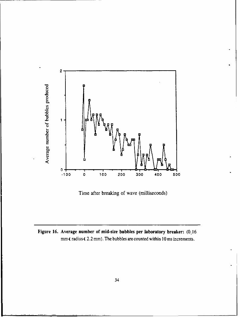
Figure 16. Average number of mid-size bubbles per laboratory breaker: (0. 16m radius ( 2.2 mm). The bubbles are counted within 10 ms increments.

34

.)

-

C

003-U

.0E

.10 0 100o 200 300 400 500

Time after breaking of wave (milliseconds)

Figure 17. Average number of small bubbles per laboratory breaker: (l "jius C0.16 mm). The bubbles are counted within 10 ms increments.

35

E. BUBBLE PRODUCTION DENSITY

The rate at which bubbles will be produced is related to the foam coverage. With

this knowledge researchers will be better able to understand the phenomena which affect

acoustics, weather, aerosol production, and any other seasurface interactions. The two

major requirements for density calculations have already been covered: the bubble cre-

ation rate relative to the start of the breaking of the wave, and the area over which these

bubbles are being produced.

All bubbles in figures (15) - (17) with equal radii were summed and the average

number of bubbles per breaker with that radius was computed by dividing by the num-

ber of waves observed. In an earlier experiment it was found that only 3 percent more

bubbles originated in the second 500 milliseconds after the breaking of the wave. Because

the measurements were again taken over a period of 500 milliseconds the number of

bubbles observed was thus increased by 3 percent to give the number of bubbles in the

first second. This number is now defined as the "total" number of bubbles. In an addi-

tional earlier experiment it was found that the average area of bubble production

spanned 345 square centimeters or equivalently 0.0345 square meters. The "total"

number of bubbles was divided by 0.0345 to give the resulting average bubble production

density in bubbles per square meter for each bubble radius observed. Thus the bubble

production will be expressed in bubbles per square meter and assumes negligible num-

bers of bubbles are formed beyond the first second after the wave breaks.

Bubbles were observed with finite numbers of different size radii. If an infinite

number of waves were measured, eventually bubbles would be observed having every

possible radius up to the maximum gas volume that can physically be encapsulated. To

account for this linitation in the data recorded, the span in bubble radius in microns

was calculated to include half the bubble radius size between each of the subsequent

smaller and larger bubble observations. The number of bubbles per square meter was

divided by this radius span to give the bubble density in bubbles per square meter per

micron of bubble radius increment.

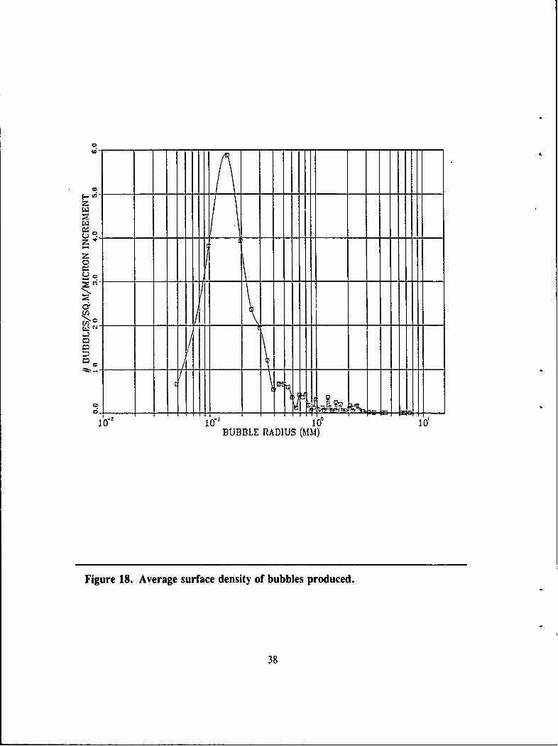
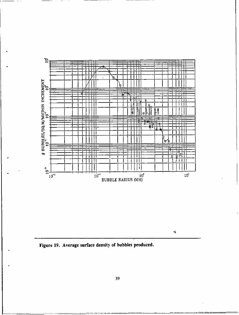
The bubble production density is plotted on semilog paper with the radius on a

logarithmic scale in figure (18), and both bubble radius and density on a logarithmic

scale in figure (19). It can be seen that the most conmmonly produced bubble was 0.15

nmm in radius produced at the approximate density of 5.9 bubbles per square meter per

micron radius increment. The smallest bubble radius measured was 0.048 mm which has

a corresponding resonance frequency of 66 kHz. The largest bubble was of radius 7.4

36

mm with a corresponding resonance frequency of 440 1Iz. It will be assumed that still

larger bubbles would not have been found even if more breakers had been observed.

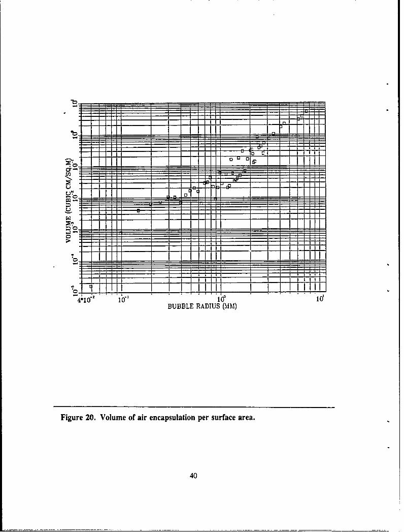
Once the production density of bubbles for each radius has been calculated the vol-

ume of gas encapsulated from each known bubble radius can be computed. Figure (20)

is a summary of cubic centimeters of gas volume encapsulated per square meter of

breaking wave for bubbles of various radii. Although it was seen in figures (18) and (19)

that the majority of bubbles produced were less than 0.5 mm in radius, the contribution

to total gas entrainment from these small bubbles is minimal. Assuming that there are

no bubbles larger than the largest measured in 10 breakers which had a radius of 7.4

nun, the individual contributions from each bubble radius can be summed to give a

volume rate of gas encapsulation which averages 23 cubic centimeters of gas

encapsulated per square meter of breaking wave in the laboratory. More than half of

this total volume came from bubbles with radius greater than 3 millimeters.

37

C

z

0

CI *1,

C - -- -o -o" o -o

102 110BUBBLE RADIUS (MM)

Figure 18. Average surface density of bubbles produced.

38

C-,

BUBBLE RADIUS (MIN)

Figure 19. Average surface density of bubbles produced.

39

--

__=___=

- _ _ _ _ _ _ _ _---

_ _ _I

___ ___L1

4010: id b ," ; OBUBBLE RADIUS (INII)

Figure 20. Volume of air encapsulation per surface area.

40

V. COMPARISON WITH OTHER DETERMINATIONS

We know of only one other attempt to measure the bubble production in a spilling

breaker, that was by Toba (1961). Contrary to our breakers being produced by an os-

cillating wedge with no wind, Toba used wind of different speeds and fetch in a flume.

Toba's method considered that an equilibrium existed between the bubbles entering fromperiodic breaking at the water surface and those rising to the surface. His photographs

were made of the volume density of bubbles, not the surface production density of the

bubbles which is our goal. He used the time between breakers to infer the bubble

encapsulation rate using the relationship

P =( (l--) 0

where i is the bubble encapsulation rate in bubbles:square cm.second, Cl. is the per-100

centage of crests actually entraining bubbles, 0 is the total number of bubbles of a par-

ticular size in a water column of unit base area, and T is the period of the main surface

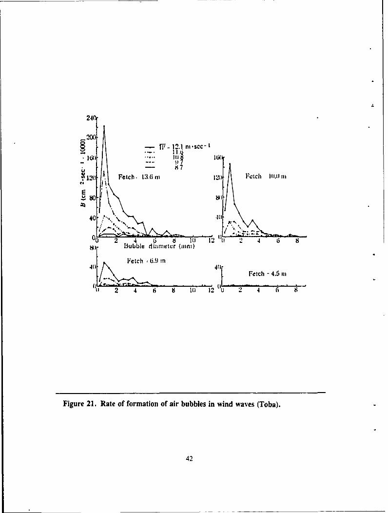
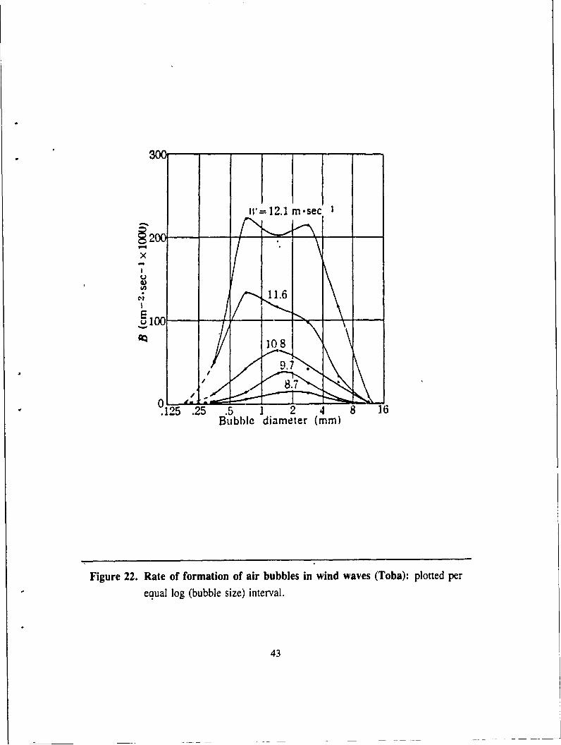
wave. The shape of'Toba's encapsulation spectrum, figures (21) and (22), was very sim-ilar to that in this experiment with a sharp peak at a single bubble radius. However the

peak of Toba's bubble production was at approximately 0.38 mm in radius at a rate ofapproximately 0.2 bubbles per square centimeter per second for a wind speed 12.1 m'sec.

His photographic measurements included 6 different sizes of bubbles with radii from 0.15

nun to 6.0 mi. Our method observed 53 bubble radii from 0.048 nm to 7.4 nm. His

smallest radius bubble was our most common bubble. The production rate inferred by

Toba for 12.1 m.sec wind was of the same order as the rate measured directly acous-

tically.There have been extensive measurements of the foam coverage at sea using aerial

photography and satellite imaging. The foam coverage is a measurement of residual

bubbles including those convected upward from below and lacking those that have beenconvected from the surface to lower depths or that have burst at the surftce. Thus the

area of coverage can not be used directly with the densities measured in this experiment

to calculate the bubble populations beneath the ocean surface. Further experimentation

is required in order to understand exactly what is being measured from the foam of

breaking waves.

41

24n

W, I"" 12.1 ni scc

87U A Fetch. 13.(6 87 12J Fetch 10.0 111

Ul so8.

'I'40 ... .

VO 2 4 6 6 11) 12 2 4 6 8N ). Bubbk diameter (mm)

Fetch 6.9 in41)' 4140, 4( Fetch - 4.5 In

2 4 6 8 M12 2U 2 4 (

Figure 21, Rate of formation of air bubbles in wind waves (Toba).

42

I1'=12.1m-sec 1

x7

C 111.6

EU 100

Q4 108

0 Z

.15.25 .5 1 2 4 8 16Bubble diameter (mm)

Figure 22. Rate of formation of air bubbles in wind waves (Toba): plotted per

eaual log (bubble size) interval.

43

VI. CONCLUSIONS

The method described throughout this thesis achieved its goal of obtaining the

bubble production density from plunger generated spilling breakers. The technique usedwas to passively observe the amplitude and frequency of the randomly pulsed sound

emitted by the breakers. The results give more details of the characteristics of bubble

production than previous experimental techniques used for obtaining surface bubble

densities.

Bubbles were positively identified throughout a radius range of 0.048 to 7.4 milli-

meters. Most of the bubbles originate in the first 500 milliseconds after the breaking of

the wave though sound from bubbles has been recorded for a period of 2 to 3 seconds

after breaking. The bubbles were produced with an exponentially decreasing rate fol-

lowing a decay constant of-0.007t with time measured in milliseconds after the breaking

of the wave. The average area of bubble production from breaking waves in the tankwas 3-45 square centimeters. The most comnmonly produced bubble had a radius of 0.15

millimeters and was entrained at a density of 5.9 bubbles per square meter per micron

of bubble radius increment. This bubble radius is smaller than the ninimum bubble ra-

dius measured in other experiments using photographic techniques to obtain bubblevolume density. The greater resolution using acoustics instead of photography has al-

lowed 10 times the resolution in bubble radii identification for bubbles with radii be-

tween 0.25 and 2.0 millimeters. The average encapsulation of gas was 23 cubic

centimeters per square meter of breaking wave.Using the Knudsen sound radiated from the breaking waves as our sole criterion,

whitecaps from spilling ocean waves have little physical difference fi'om the breakingwaves produced in the laboratory. If' this is the case, the measurements reported here

are useable for the ocean. The use of this passive acoustical technique in actual sea

measurements may also be possible. If these laboratory data are confirmed by actual

measurements of surflace bubble production density at sea, and after further studies ofbubble dissipation in a turbulent ocean, satellite measurements of the foam coverage

from whitecaps could yield an estimate of t'.e rate of bubble production in the ocean.

44

APPENDIX A. EVIDENCE OF CAPILLARY WAVES

Upon examination of the bubble location plots it was discovered that in some of the

plots the bubbles appeared to be located along lines perpedicular to the wave propa-

gation direction (fig 12) and in other cases the lines are not perpendicular to the direction

of wave propagation. These lines appeared with varying angles ranging from 30 to 90

degrees away from the propagation direction. It was hypothesized that these may have

been capillary waves forming on the face of the main wave. A purely arbitrary reference

time of 10 milliseconds was chosen as the time within which all of the bubbles on the line

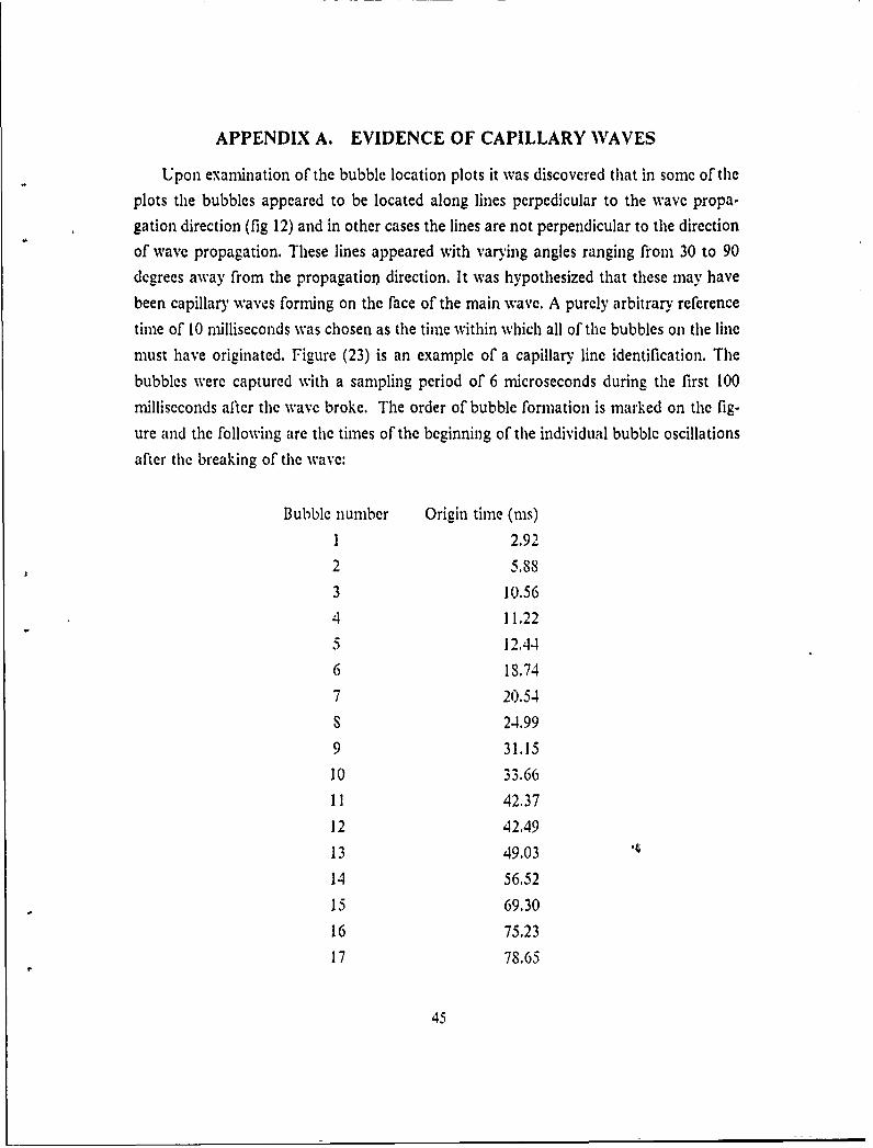
must have originated. Figure (23) is an example of a capillary line identification. Thebubbles were captured with a sampling period of 6 microseconds during the first 100

milliseconds after the wave broke. The order of bubble formation is marked on the fig-

ure and the following are the times of the beginning of the individual bubble oscillations

after the breaking of the wave:

Bubble number Origin time (mis)

1 2.92

2 5.88

3 10.56

4 11.22

.5 12.44

6 18.74

7 20.54

S 24.99

9 31.15

10 33.66

11 42.37

12 42.49

13 49.03

14 56.52

15 69.30

16 75.2317 78.65

45

18 80.45

19 81.83

20 93.94

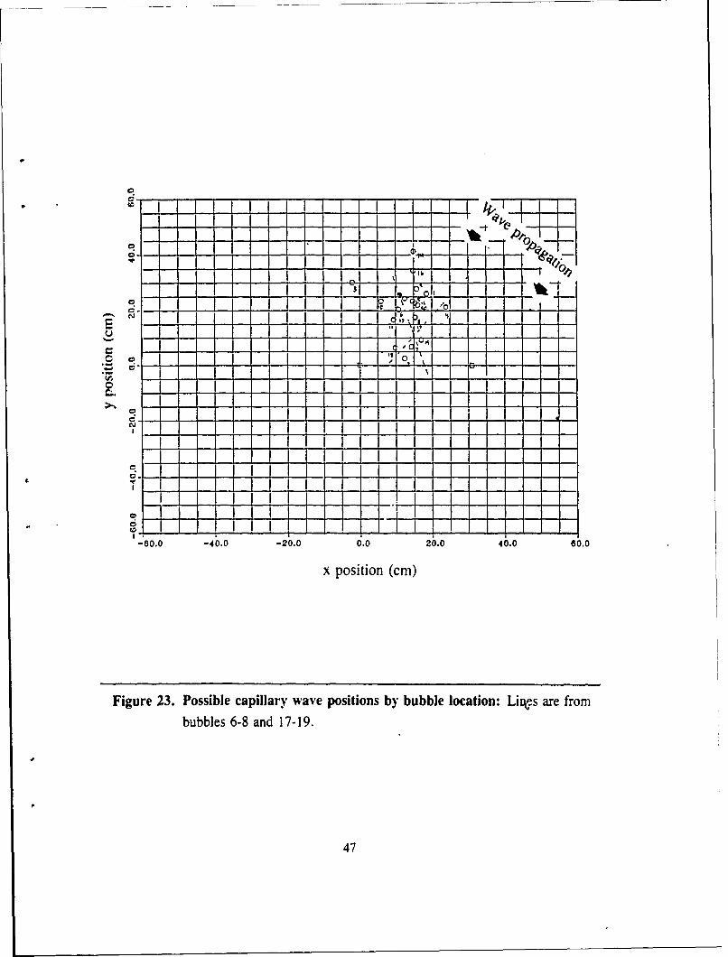
The capillary lines on figure (23) are identified by bubbles 6 through 8 and by bubbles

17 through 19. Figures (24) and (25) are photographs of breaking waves in which the

capillary waves may be cleariy observed.

46

0

p . -. I- -TIz- I

0 .-D I

,.

Er,

-60.0 -40.0 -20.0 0.0 20.0 40.0 606

x position(m

Figure 23. Possible capillary wave positions by bubble location: Liqes are from

bubbles 6-8 and 17-19.

47

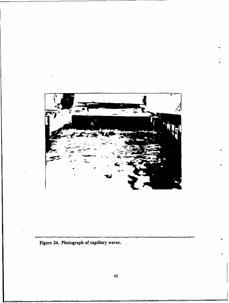
Figure 24. Photograph of capillary waves.

48

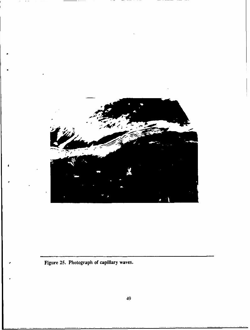
Figure 25. Photograph of capillary waves.

49

APPENDIX B. VOLTAGE AMPLIFIERS

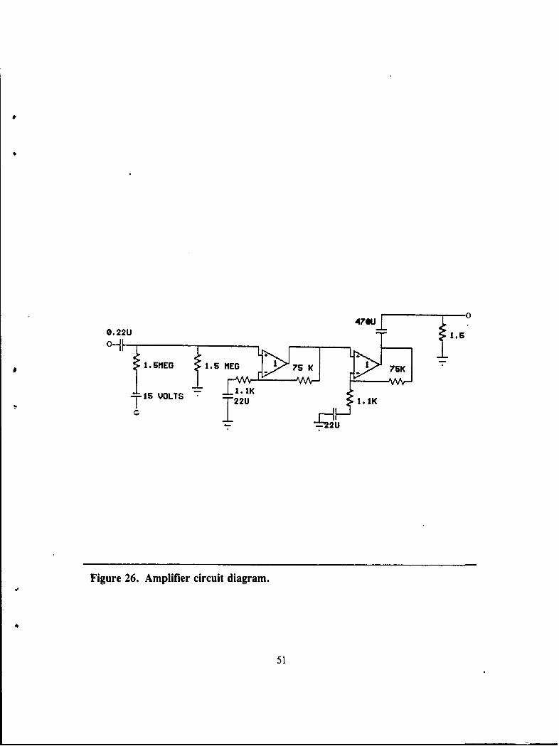
When receiving signals from many hydrophones simultaneously, it was necessary to

develop a substitute for the limited number of Ithaco 1201 Preamplifiers. A series of

preamplifiers was built using two 356 operational amplifiers in series with the necessary

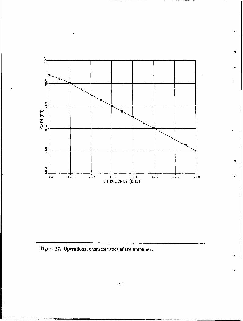
feedback elements. Figure (26) is the diagram of the amplifier circuit. Figure (27) shows

the operational characteristics of the amplifier.

so

0. 22U 1 K7 1.600

16 VOLTS221.I

Figure 26. Amplifier circuit diagram.

51

Co

cc_ _ _ __ _ _ _ _

0.0 1. 603 65. 007.

FRQENYoKZ

Fiue2.O eainlcaaceitc0ftea piir

C.52

LIST OF REFERENCES

Breitz, N., and Medwin, H., "Instrumentation for in situ Acoustical Measurements ofBubble Spectra under Breaking Waves," J. Acoust. Soc. Am., v. 86 pp. 739-743, 19S9.

Clay, C.S., and Medwin, H., Acoustical Oceanography: Principles and Applications, John

Wiley and Sons, New York, p. 196, 1977.

Farmer, D. M., and Vagle, S., "Waveguide propagation of ambient sound in the ocean-

surface bubble layer," J. Acoust. Soc. Am., v. 86 pp. 1897-1908, 1989.

.Guchinski, H., "Bubble Coalescence in Sea and Freshwater: Requisites for an Explana-

tion," E.C. Monahan and G. Mac Niocaill (Eds.), Ocean 1Vhziecaps, p. 270, D. Reidel

Publishing Company, 1986.

Holthuijsen, L. I L. and Herbers, T. H. C., "Statistics of Breaking Waves Observed as

Whitecaps in the Open Sea," J. Phys. Ocean., v. 16 pp. 290-297, 1986.

Johnson, B. D., and Cooke, R. C., "Bubble Populations in Coastal Waters: A Photo-

graphic Approach," J. Geopis. Res., v. 84 pp. 3761-3766, 1979.

Kolovaycv. D. A., "Investigation of the Concentration and Statistical Size Distribution

of Wind-Prodticed Bubbles in the Near-Surface Ocean," Oceanology, v. 15 pp. 659-661,

1976.

Levich, V. G., Physiochemical lydrodynanfics, Prentice Hall, 1962.

Longuet-liggins, M. S., "Bubble Noise Spectra," J. Acoust. Soc. Am., (submitted), 1989.

Medwin, H., and Beaky. M. M., "Bubble Sources of the Knudsen Sea Noise Spectra,"

J. Acoust. Soc. Anz., v. 86 pp. 1124-1130, 1989.

53

Miller, R. L., University of Chicago, Fluid Dynamics and Sediments Transport Labora-

tory, Dept. of Geophysical Sciences, Technical Report No. 13, 1972.

Morse, P. M., and Ingard, K. U., Theoretical Acoustics, McGraw-Hill, New York, 1968.

Toba, Y., and Koga, K., "A Parameter Describing Overall Conditions of Wave Breaking,Whitecapping, Sea-Spray Production, and Wind Stress," E. C. Monahan and G. Mac

Niocaill (Eds.), Ocean W1'hitecaps, pp. 37-47, D. Reidell Publishing Company, 19S6.

Toba, Y., "Drop Production by Bursting of Air Bubbles on the Sea Surface (III) Study

by Use of a Wind Flume," Memoirs of the College of Science, University of Kyoto, Series

A, v. XXIX, No. 3, Art. 4, pp. 313-344, 1961.

Thorpe, S. A., "Bubble Clouds: A Review of Their Detection by Sonar, of Related

Models. and of How K, may be Determined," E. C. Monahan and G. Mac Niocaill

(Eds.), Ocean Whitecaps, pp. 57-68, D. Reidell Publishing Company, 1986.

Thorpe, S. A., and I lall, A. J., "The Characteristics of Breaking Waves, Bubble Clouds,

and Near-Surface Currents Observed Using Side-Scan Sonar," Cominental Shelf Re-

search, v. I pp. 353-384, 19S3.

Urick, R. J., Principles of U-nderwater Sound, 3rd Edition, McGraw-I ll Book Company,

1983.

544

54 r --, - . . ,

INITIAL DISTRIBUTION LIST

No. Copies

1. Defense Technical Information Center 2Cameron StationAlexandria, VA 22304-6145

2. Library, Code 0142 2Naval Postgraduate SchoolMonterey, CA 93943-5002

3. Prof H. Mcdwin (Code 61Md) 6Department of PhysicsNaval Postgraduate SchoolMonterey, CA 93943-5004

4. ProfJ. A. Nystuen 2Dcpartment of OceanographyNaval Postgraduate SchoolMonterey, CA 93943-5004

5. Commanding Officer 3Attn: LT A. C. I)anielUSS Devo (DD-989)FPO Miami. FL 34090-1227

6. Office of Naval ResearchAttn: Dr. Marshall Orr800 N. QuincyArlington, VA 22217

7. ProfA. A. AtchleyDepartment of hy'sicsNaval Postgraduate SchoolMonterey, CA 93943-5004

8. David M. FarmerInstitute of Ocean SciencesP. 0. Box 6000Sidney. Bi'itish Columbia, V8L4B2Canada

9. M. S. Longuet-l-figgins ICenter for Studies of Nonlinear DynamicsLa Jolla Institute7855 Fay Avenue. Suite 320La Jolla, CA 92037

55

10. S. A. ThorpeInstitute of Oceanographic SciencesWormley , Godalming, Surrey GU85UBUnited Kingdom

11. E. C. MonohianMarine Sciences InstituteUnivcrsity of ConnecticutAvery Point

*Groton, CT 06340

56