arX

iv:1

001.

5208

v1 [

gr-q

c] 2

8 Ja

n 20

10

The Robertson-Walker Metric in a

Pseudo-complex General Relativity

Peter O. Hess1, Leila Maghlaoui2 and Walter Greiner2

1Instituto de Ciencias Nucleares, UNAM, Circuito Exterior, C.U.,

A.P. 70-543, 04510 Mexico D.F., Mexico

2Frankfurt Institute for Advanced Studies, Johann Wolfgang Goethe Universitat,

Ruth-Moufang-Str. 1, 60438 Frankfurt am Main, Germany

September 12, 2018

Abstract

We investigate the consequences of the pseudo-complex GeneralRelativity within a pseudo-complexified Roberston-Walker metric. Acontribution to the energy-momentum tensor arises, which correspondsto a dark energy and may change with the radius of the universe, i.e.,time. Only when the Hubble function H does not change in time, thesolution is consistent with a constant Λ.

PACS: 02.40.ky, 98.80.-k

1 Introduction

In the past several paths have been proposed on how to extend thetheory of General Relativity (GR). One of the first was Einstein himself[1, 2] who, in an attempt to unify electrodynamics with GR, extendedGR to complex GR. For more recent articles on complex GR, you mayconsult [3, 4]. Others [5, 6, 7, 8, 9, 10, 11, 12, 13, 14, 15] introduceda maximal acceleration, related to a minimal length parameter in thetheory, or [16, 17, 18, 19] tried to extend GR by introducing hyperboliccoordinates.

1

The introduction of a maximal acceleration and the use of hy-percomplex (a synonym for para-complex) coordinates is very muchrelated to what was published in [20]. In [20] a pseudo-complex (pc)extension of General Relativity (GR) was proposed. (To the article[20] we will refer from here on as (I).) The main objective was to inves-tigate the analogue of the Schwarzschild metric and its consequenceswithin the pseudo-complex extension of GR. Its possible experimentalverification was and is of prime importance. The pc-GR is formulatedin a different manner than in [16, 17, 18, 19]. Because pseudo-complexnumbers exhibit a zero divisor basis (see section II), we were able todefine two independent theories of GR in each zero-divisor component,which were later connected. The resulting length squared element issimilar but not equal to [5, 6, 7, 8, 9, 10, 11, 12, 13, 14, 15]. It containsan additional term proportional to the velocity times acceleration. Asalready said, the analogue of the Schwarzschild solution was studiedwithin the new formalism. A strong heuristic assumption was made,requiring that the pc scalar curvature R = 0. This did lead to strongcorrections, which are excluded by the Parametrized-Post-Newton for-

malism (PPN) [21]. However, relaxing the condition gives correctionswhich are smaller and not contradicting the PPN formalism; detailswill be given in a forthcoming publication. Deviations of the redshiftto the standard Schwarzschild case were calculated.

One of the main results and messages in (I) was: The pseudo-complex description, with its extended variational principle, containsno singularity, i.e. black holes don’t exist. Furthermore, the new the-ory (I) automatically introduces dark energy, whose density dependsin the analogue of the Schwarzschild case on the radial distance. Infact, the increase of the dark energy density towards smaller radialdistances finally hinders (prevents) the collapse of a large mass. Theincrease of dark energy, as a function of the radial distance, dependssensitively on some functions ξk, which are very difficult to deduce.The results are in line with the model described in [22] where the darkenergy is described by a scalar field coupled to gravity. It is interestingand quite helpful for understanding, to compare our results with thoseobtained within this model. In the model [22] the relativistic equa-tions are solved numerically. As a result, dark energy accumulatesaround the central mass, reducing the radius of the event horizon.The advantage of this model [22] is that it provides a distribution ofthe scalar field, whose intensity should be proportional to our ξ func-tions. In one case, the dark energy falls off very quickly with the radial

2

distance. The disadvantage is the large numerical effort needed. Thesimilarity between this procedure and our theory, however, indicatesthat both investigations might be useful for each other.

Here, in this contribution, we intend to show that the same effectintroduces a dark energy in models of the Robertson-Walker (RW)type universes [29, 28]. Our theory also contains a minimal lengthscale. Its influence on solutions might be important for large massconcentrations [23]. Here, we will not discuss it but refer to a laterpublication. Whether our theory is realized in nature also depends onthe predictions which can be made and on their experimental verifica-tion. In the present contribution our principal objective is to identifysome consequences of the pseudo-complex theory, and to determinewhether possible differences to Einsteins General Relativity may beobserved.

In section II a short review on how to define pc variables and theirproperties will be given. This is for those readers who are not yetaccustomed to this mathematical structure. A simple presentation canalso be found in (I). In section III we will formulate the pc extensionof the Robertson-Walker metric. It will be quite straight forward andthe steps can be copied from [29] or any other book on GR may beconsulted. For details, we will give mainly reference to [29]. In sectionIV we will solve the pc-RW model and in section V we shall discusssome consequences. Section VI summarizes the main conclusions.

2 Pseudo-complex variables and pseudo-

complex metric

Here we give a brief resume on pseudo-complex variables, helpful tounderstand various steps presented in this contribution. The formulas,presented here, can be used without going into the details. A moreprofound introduction to pseudo-complex variables is given in [24, 25],which may be consulted for better understanding.

The pseudo-complex variables are also known as hyperbolic [16, 17],hypercomplex [26] or para-complex [27]. We will continue to use theterm pseudo-complex.

The pseudo-complex variables are defined via

X = x1 + Ix2 , (1)

3

with I2 = 1. This is similar to the common complex notation ex-cept for the different behavior of I. An alternative presentation is tointroduce the operators

σ± =1

2(1± I)

(2)

with

σ2± = σ± , σ+σ− = 0 . (3)

The σ± form a so called zero divisor basis, with the zero divisor definedin mathematical terms by P

0 = P0+∪P 0

−, with P0± = X = λσ±|λ ǫ R.

The zero divisor generates all the differences to the complex number.This basis is used to rewrite the pseudo-complex variables as

X = X+σ+ +X−σ− , (4)

with

X± = x1 ± x2

or

x1 =1

2(X+ +X−) , x2 =

1

2(X+ −X−) . (5)

The pseudo-complex conjugate of a pseudo-complex variable is

X∗ = x1 − Ix2 = X+σ− +X−σ+ . (6)

The norm square of a pseudo-complex variable is given by

|X|2 = XX∗ = x21 − x22 = X+X− . (7)

This allows for the appearance of a positive, negative and null norm.Variables with a zero norm are members of the zero-divisor, i.e., theyare either proportional to σ+ or σ−.

It is very useful to carry out all calculations within the zero divisor

basis, σ±. Here, all manipulations can be realized independently in

both sectors, because σ+σ− = 0.

4

In each zero divisor component, differentiation and multiplicationcan be manipulated in the same way as with real or complex variables.For example, we have [25]

F (X) = F (X+)σ+ + F (X−)σ− (8)

and a product of two functions F (X) and G(X) satisfies

F (X)G(X)

= (F (X+)σ+ + F (X−)σ−) (G(X+)σ+ +G(X−)σ−)

= F (X+)G(X+)σ+ + F (X−)G(X−)σ− , (9)

because σ+σ− = 0 and σ2± = σ±. As a further example, we have

F (X)

G(X)=

F (X+)

G(X+)σ+ +

F (X−)

G(X−)σ− . (10)

This can be proved as follows:

F (X)G(X) =

F (X+)σ++F (X−)σ−

G(X+)σ++G(X−)σ−

= (F (X+)σ++F (X−)σ−)(G(X+)σ−+G(X−)σ+)(G(X+)σ++G(X−)σ−)(G(X+)σ−+G(X−)σ+) (11)

where we have multiplied the numerator and denominator by thepseudo-complex conjugate of G(X), using σ∗

+ = σ−. With σ+σ− = 0and σ2

± = σ±, the last expression can be written as

(F (X+)G(X−)σ++F (X−)G(X+)σ−)G(X+)G(X−)(σ++σ−) . (12)

Because σ+ + σ− = 1, we arrive at Eq. (10).Differentiation is defined as

DF (X)

DX= lim

∆X→0

F (X +∆X)− F (X)

∆X, (13)

where D refers from here on to the pseudo-complex infinitesimal dif-ferential.

5

A very important difference to the standard GR is the introductionof a modified variational principle. It states that the variation of anaction has to be within the zero-divisor, i.e.

δS ǫ P0 , (14)

where P0 denotes the zero divisor given by all values which are eitherproportional to σ+ (λσ+) or to σ− (λσ−). For convenience, the latteris chosen in this contribution, as it was in (I). However, instead of”ǫ P0” we write here ”= λσ−”. The number at the right hand side of(14) has zero norm and can be treated as a ”generalized zero”, thusrepresenting a minimal extension of the variational principle.

In the pc-GR the metric is pseudo-complex, i.e., (see (I) for details)

gµν = g+µνσ+ + g−µνσ− . (15)

Each component (σ±) can be treated independently, for many pur-poses, e.g., as how to define parallel displacement, Christoffel symbols,etc. Most of the steps, known from standard GR can be carried outanalogously. This is the advantage of using the zero-divisor basis. Itcan also be shown that the four-divergence of the metric tensor is zero(see (I)).

The connection of both components of the zero-divisor basis hap-pens through the variation principle, mentioned above. It states that,with the convention used and δS = δS+σ+ + δS−σ−, we have

δS+ = 0 and δS− = λ . (16)

For the length element square

dω2 = gµνDXµDXν

= g+µνDXµ+DXν

+σ+ + g−µνDXµ−DXν

−σ+

= DX+µ DXµ

+σ+ +DX−µ DXµ

−σ− , (17)

reality is imposed through

dω∗2 = dω2 . (18)

6

This implies that dω2 is equal to its pseudo real part

dω2 =1

2

(DX+

µ DXµ+ +DX−

µ DXµ−

)

= dxµdxµ + l2duµdu

µ (19)

where in the last step we simply substituted X±µ and Xµ

± by their ex-pressions in terms of the coordinates and four-velocities. The pseudo-imaginary component has to vanish, i.e.,

0 =1

2

(DX+

µ DXµ+ −DX−

µ DXµ−

)

= l (dxµduµ + duµdx

µ) . (20)

One way to proceed is to take (19) as the final length element andimpose (20) as a constriction, noting that (20) gives the dispersionrelation: Integrating, this gives uµu

µ = 1. This is a nice featurebecause in other models the dispersion relation is usually put in byhand.

Using Eq. (37) of (I), which reads in differential form

dxµ = g0µνdxν + lhµνdu

ν

lduµ = lg0µνduν + hµνdx

ν , (21)

the length element (19) and the constriction (20) can be respectivelywritten as

dω2 = g0µν(dxµdxν + l2duµduν)

+lhµν(dxµduν + duµdxν) ,

(22)

and

hµν(dxµdxν + l2duµduν

)

+lg0µν (dxµduν + duµdxν) = 0 . (23)

These are the expressions reported in (I).

7

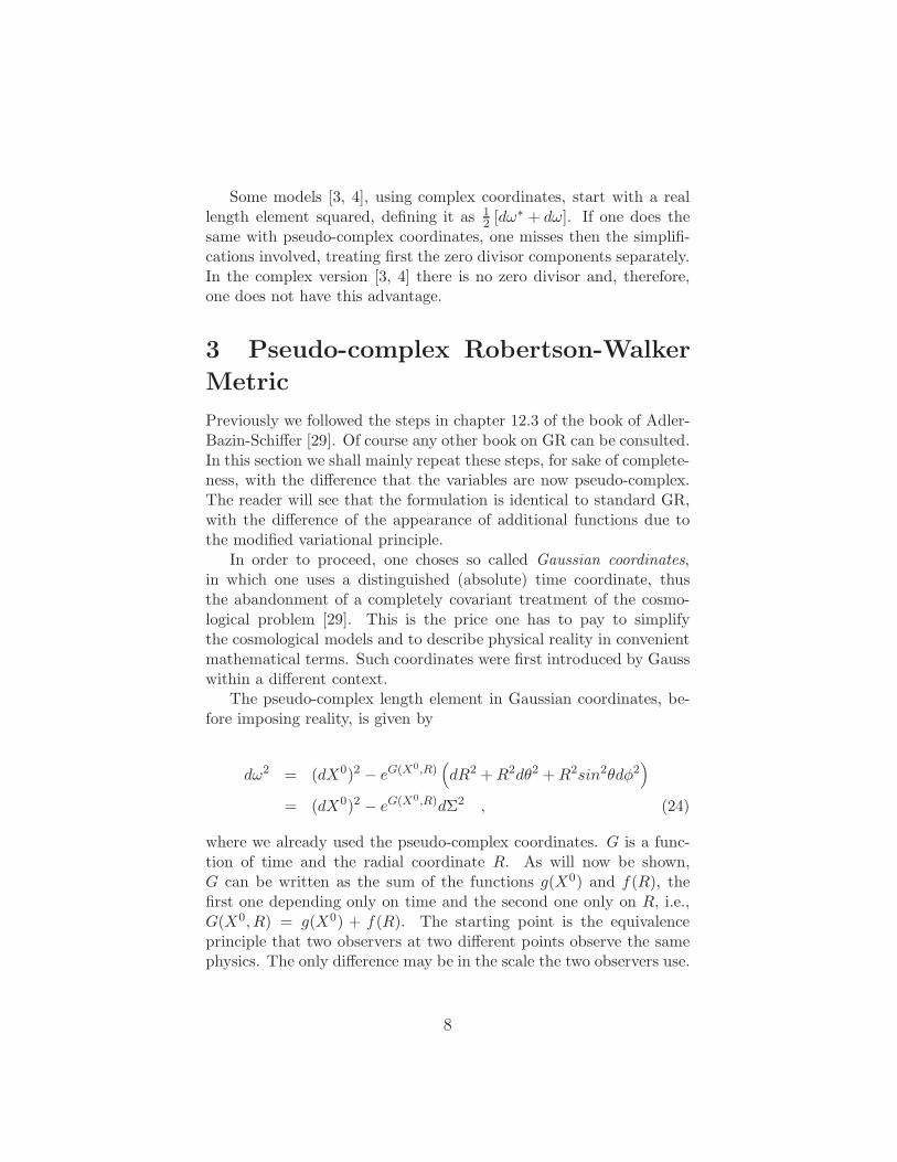
Some models [3, 4], using complex coordinates, start with a reallength element squared, defining it as 1

2 [dω∗ + dω]. If one does the

same with pseudo-complex coordinates, one misses then the simplifi-cations involved, treating first the zero divisor components separately.In the complex version [3, 4] there is no zero divisor and, therefore,one does not have this advantage.

3 Pseudo-complex Robertson-Walker

Metric

Previously we followed the steps in chapter 12.3 of the book of Adler-Bazin-Schiffer [29]. Of course any other book on GR can be consulted.In this section we shall mainly repeat these steps, for sake of complete-ness, with the difference that the variables are now pseudo-complex.The reader will see that the formulation is identical to standard GR,with the difference of the appearance of additional functions due tothe modified variational principle.

In order to proceed, one choses so called Gaussian coordinates,in which one uses a distinguished (absolute) time coordinate, thusthe abandonment of a completely covariant treatment of the cosmo-logical problem [29]. This is the price one has to pay to simplifythe cosmological models and to describe physical reality in convenientmathematical terms. Such coordinates were first introduced by Gausswithin a different context.

The pseudo-complex length element in Gaussian coordinates, be-fore imposing reality, is given by

dω2 = (dX0)2 − eG(X0,R)(dR2 +R2dθ2 +R2sin2θdφ2

)

= (dX0)2 − eG(X0,R)dΣ2 , (24)

where we already used the pseudo-complex coordinates. G is a func-tion of time and the radial coordinate R. As will now be shown,G can be written as the sum of the functions g(X0) and f(R), thefirst one depending only on time and the second one only on R, i.e.,G(X0, R) = g(X0) + f(R). The starting point is the equivalenceprinciple that two observers at two different points observe the samephysics. The only difference may be in the scale the two observers use.

8

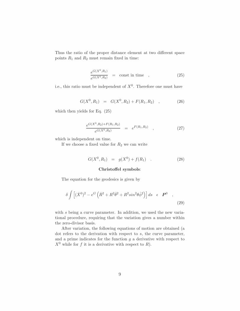
Thus the ratio of the proper distance element at two different spacepoints R1 and R2 must remain fixed in time:

eG(X0,R1)

eG(X0,R2)= const in time , (25)

i.e., this ratio must be independent of X0. Therefore one must have

G(X0, R1) = G(X0, R2) + F (R1, R2) , (26)

which then yields for Eq. (25)

eG(X0,R2)+F (R1,R2)

eG(X0,R2)= eF (R1,R2) , (27)

which is independent on time.If we choose a fixed value for R2 we can write

G(X0, R1) = g(X0) + f(R1) . (28)

Christoffel symbols:

The equation for the geodesics is given by

δ

∫ [(X0)2 − eG

(R2 +R2θ2 +R2sin2θφ2

)]ds ǫ P

0 ,

(29)

with s being a curve parameter. In addition, we used the new varia-tional procedure, requiring that the variation gives a number withinthe zero-divisor basis.

After variation, the following equations of motion are obtained (adot refers to the derivation with respect to s, the curve parameter,and a prime indicates for the function g a derivative with respect toX0 while for f it is a derivative with respect to R).

9

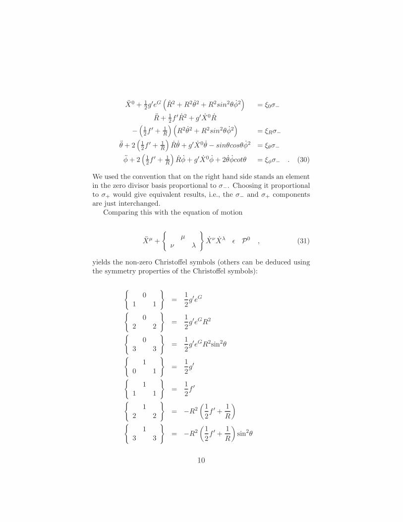
X0 + 12g

′eG(R2 +R2θ2 +R2sin2θφ2

)= ξ0σ−

R+ 12f

′R2 + g′X0R

−(12f

′ + 1R

) (R2θ2 +R2sin2θφ2

)= ξRσ−

θ + 2(12f

′ + 1R

)Rθ + g′X0θ − sinθcosθφ2 = ξθσ−

φ+ 2(12f

′ + 1R

)Rφ+ g′X0φ+ 2θφcotθ = ξφσ− . (30)

We used the convention that on the right hand side stands an elementin the zero divisor basis proportional to σ−. Choosing it proportionalto σ+ would give equivalent results, i.e., the σ− and σ+ componentsare just interchanged.

Comparing this with the equation of motion

Xµ +

µ

ν λ

XνXλ ǫ P0 , (31)

yields the non-zero Christoffel symbols (others can be deduced usingthe symmetry properties of the Christoffel symbols):

0

1 1

=

1

2g′eG

0

2 2

=

1

2g′eGR2

0

3 3

=

1

2g′eGR2sin2θ

1

0 1

=

1

2g′

1

1 1

=

1

2f ′

1

2 2

= −R2

(1

2f ′ +

1

R

)

1

3 3

= −R2

(1

2f ′ +

1

R

)sin2θ

10

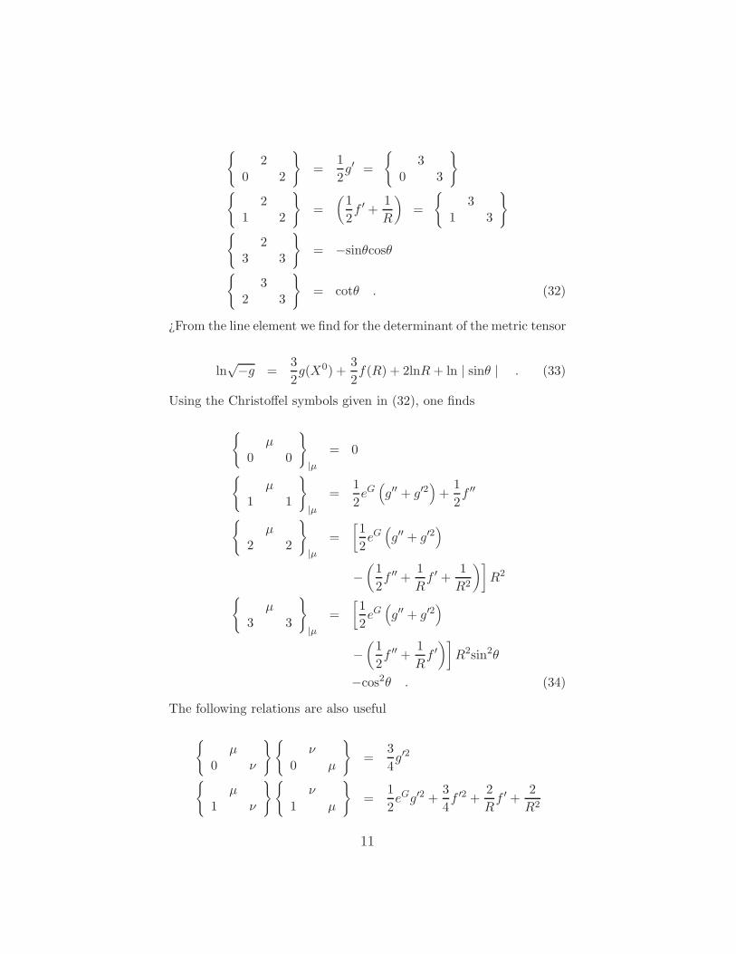
2

0 2

=

1

2g′ =

3

0 3

2

1 2

=

(1

2f ′ +

1

R

)=

3

1 3

2

3 3

= −sinθcosθ

3

2 3

= cotθ . (32)

¿From the line element we find for the determinant of the metric tensor

ln√−g =

3

2g(X0) +

3

2f(R) + 2lnR+ ln | sinθ | . (33)

Using the Christoffel symbols given in (32), one finds

µ

0 0

|µ

= 0

µ

1 1

|µ

=1

2eG(g′′ + g′2

)+

1

2f ′′

µ

2 2

|µ

=

[1

2eG(g′′ + g′2

)

−(1

2f ′′ +

1

Rf ′ +

1

R2

)]R2

µ

3 3

|µ

=

[1

2eG(g′′ + g′2

)

−(1

2f ′′ +

1

Rf ′)]

R2sin2θ

−cos2θ . (34)

The following relations are also useful

µ

0 ν

ν

0 µ

=

3

4g′2

µ

1 ν

ν

1 µ

=

1

2eGg′2 +

3

4f ′2 +

2

Rf ′ +

2

R2

11

µ

2 ν

ν

2 µ

=

[1

2eGg′2 − 1

4f ′2 − 2

Rf ′

− 2

R2+

1

R2cot2θ

]R2

µ

3 ν

ν

3 µ

=

[1

2eGg′2 − 1

2f ′2 − 2

Rf ′

− 2

R2+

1

R2cot2θ

]

×R2sin2θ . (35)

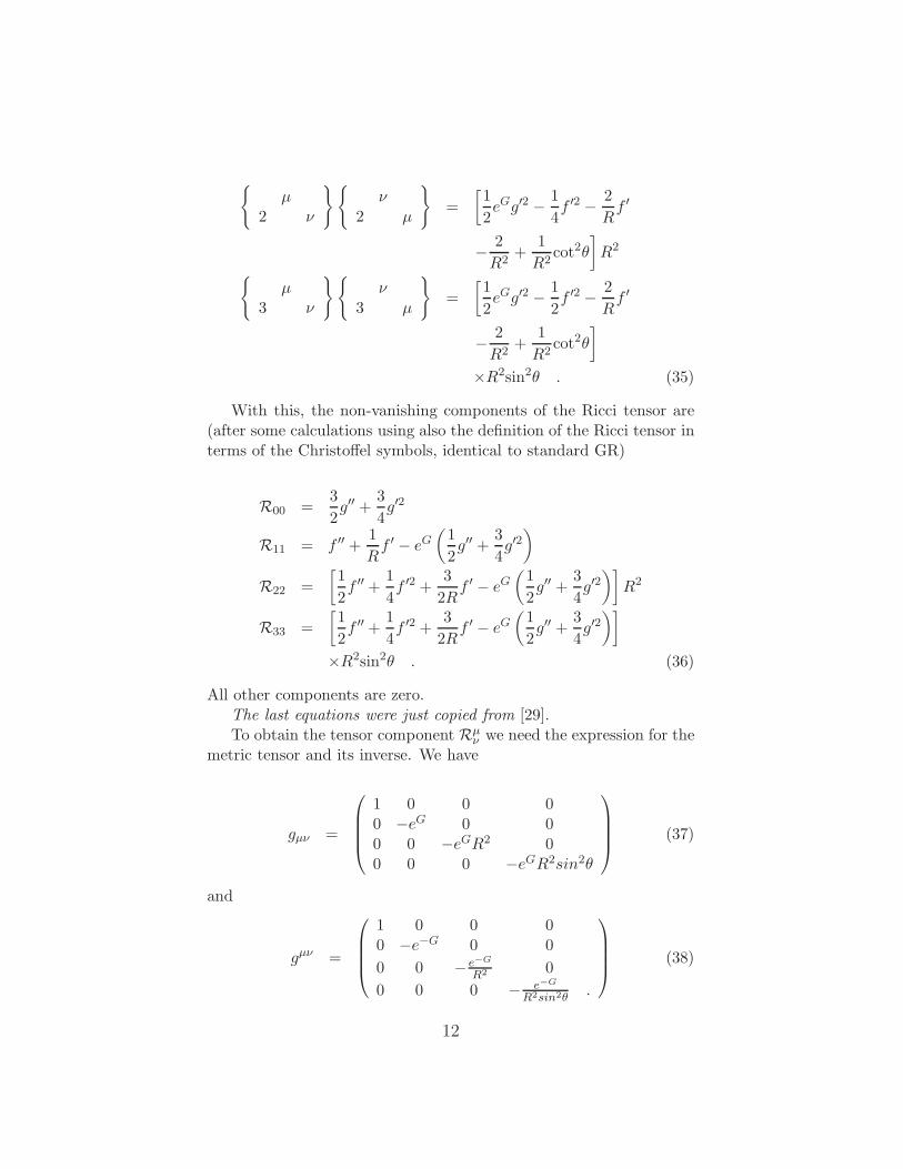
With this, the non-vanishing components of the Ricci tensor are(after some calculations using also the definition of the Ricci tensor interms of the Christoffel symbols, identical to standard GR)

R00 =3

2g′′ +

3

4g′2

R11 = f ′′ +1

Rf ′ − eG

(1

2g′′ +

3

4g′2)

R22 =

[1

2f ′′ +

1

4f ′2 +

3

2Rf ′ − eG

(1

2g′′ +

3

4g′2)]

R2

R33 =

[1

2f ′′ +

1

4f ′2 +

3

2Rf ′ − eG

(1

2g′′ +

3

4g′2)]

×R2sin2θ . (36)

All other components are zero.The last equations were just copied from [29].To obtain the tensor component Rµ

ν we need the expression for themetric tensor and its inverse. We have

gµν =

1 0 0 00 −eG 0 00 0 −eGR2 00 0 0 −eGR2sin2θ

(37)

and

gµν =

1 0 0 00 −e−G 0 0

0 0 − e−G

R2 0

0 0 0 − e−G

R2sin2θ.

(38)

12

With this we get (Rνµ = gνρRµρ)

R00 =

3

2g′′ +

3

4g′2

R11 =

(1

2g′′ +

3

4g′2)− e−G

(f ′′ +

f ′

R

)

R22 = R3

3 =

(1

2g′′ +

3

4g′2)

−e−G

(1

2f ′′ +

1

4f ′2 +

3f ′

2R

).

(39)

The Riemann curvature is then

R = 3(g′′ + g′2

)− 2e−G

(f ′′ +

f ′2

4+

2

Rf ′

)(40)

Denoting the energy momentum tensor by T µν and exploiting the

above results, the equations of motion are

− 8πκ

c2T 00 =

[e−G

(f ′′ +

f ′2

4+

2f ′

R

)− 3

4g′2]+ ξ0σ−

−8πκ

c2T 11 =

[e−G

(f ′2

4+

f ′

R

)− g′′ − 3

4g′2]+ ξ1σ−

−8πκ

c2T 22 =

[e−G

(f ′′

2+

f ′

2R

)− g′′ − 3

4g′2]+ ξ2σ−

−8πκ

c2T 33 =

[e−G

(f ′′

2+

f ′

2R

)− g′′ − 3

4g′2]+ ξ3σ−

−8πκ

c2T µν = 0 , µ 6= ν . (41)

The f ′(R) refers to the derivative with respect to R, while g′(X0)refers to the derivative with respect to X0. The ξµ functions appeardue to the new variational principle. In [29] there appears instead thecosmological constant Λ. In principle we can add such a constant,too. However, one of the reasons not to do so, is that the ξ functionswill reproduce such an effect. Inspecting Eq. (41) one can identify ξkas additional diagonal contributions to the energy-momentum tensor,

13

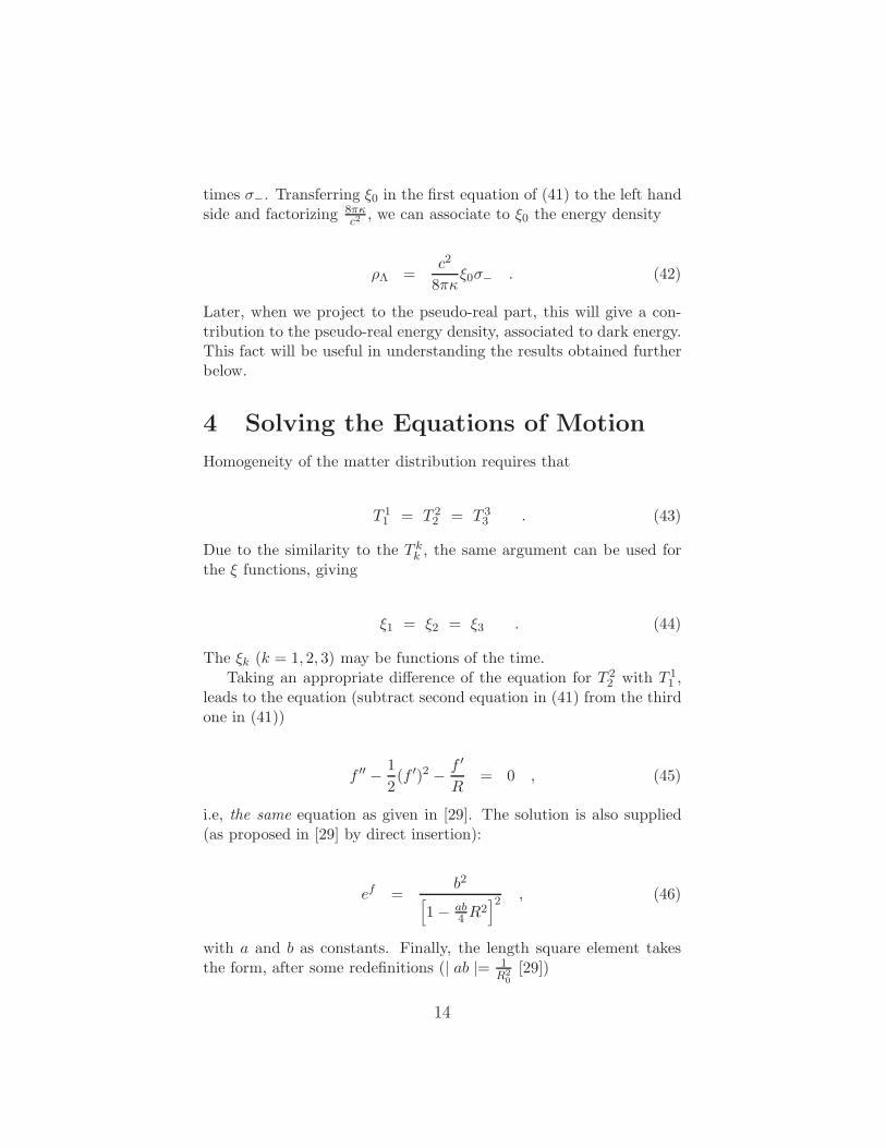
times σ−. Transferring ξ0 in the first equation of (41) to the left handside and factorizing 8πκ

c2, we can associate to ξ0 the energy density

ρΛ =c2

8πκξ0σ− . (42)

Later, when we project to the pseudo-real part, this will give a con-tribution to the pseudo-real energy density, associated to dark energy.This fact will be useful in understanding the results obtained furtherbelow.

4 Solving the Equations of Motion

Homogeneity of the matter distribution requires that

T 11 = T 2

2 = T 33 . (43)

Due to the similarity to the T kk , the same argument can be used for

the ξ functions, giving

ξ1 = ξ2 = ξ3 . (44)

The ξk (k = 1, 2, 3) may be functions of the time.Taking an appropriate difference of the equation for T 2

2 with T 11 ,

leads to the equation (subtract second equation in (41) from the thirdone in (41))

f ′′ − 1

2(f ′)2 − f ′

R= 0 , (45)

i.e, the same equation as given in [29]. The solution is also supplied(as proposed in [29] by direct insertion):

ef =b2

[1− ab

4 R2]2 , (46)

with a and b as constants. Finally, the length square element takesthe form, after some redefinitions (| ab |= 1

R20

[29])

14

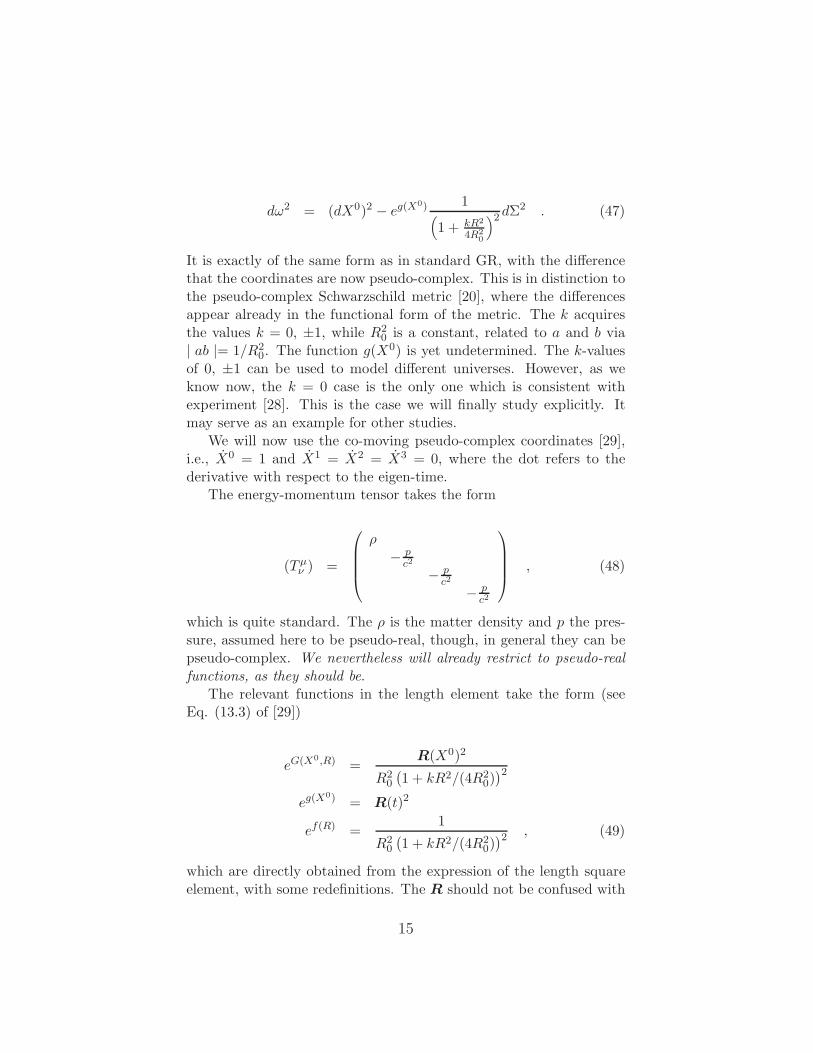
dω2 = (dX0)2 − eg(X0) 1(1 + kR2

4R20

)2 dΣ2 . (47)

It is exactly of the same form as in standard GR, with the differencethat the coordinates are now pseudo-complex. This is in distinction tothe pseudo-complex Schwarzschild metric [20], where the differencesappear already in the functional form of the metric. The k acquiresthe values k = 0, ±1, while R2

0 is a constant, related to a and b via| ab |= 1/R2

0. The function g(X0) is yet undetermined. The k-valuesof 0, ±1 can be used to model different universes. However, as weknow now, the k = 0 case is the only one which is consistent withexperiment [28]. This is the case we will finally study explicitly. Itmay serve as an example for other studies.

We will now use the co-moving pseudo-complex coordinates [29],i.e., X0 = 1 and X1 = X2 = X3 = 0, where the dot refers to thederivative with respect to the eigen-time.

The energy-momentum tensor takes the form

(T µν ) =

ρ− p

c2

− pc2

− pc2

, (48)

which is quite standard. The ρ is the matter density and p the pres-sure, assumed here to be pseudo-real, though, in general they can bepseudo-complex. We nevertheless will already restrict to pseudo-real

functions, as they should be.The relevant functions in the length element take the form (see

Eq. (13.3) of [29])

eG(X0,R) =R(X0)2

R20

(1 + kR2/(4R2

0))2

eg(X0) = R(t)2

ef(R) =1

R20

(1 + kR2/(4R2

0))2 , (49)

which are directly obtained from the expression of the length squareelement, with some redefinitions. The R should not be confused with

15

the pseudo-complex radius variable R, nor with the Riemann curva-ture R. R is an object with a length unit and is interpreted as thepseudo-complex radius of the universe.

From now on, let us substitute X0 by its pseudo-real part ct. For

example R(X0) will be written as R(t). The derivative with respect to

X0 is converted into a derivation with respect to ct, i.e., dRd(ct) = 1

cdRdt

= R′

c.

We part now from the above equations of motion (41). The ex-pressions in the functions f and g and their derivatives can be reexpressed in terms of the variable R using (49). For example f =−lnR2

0 − 2ln(1 + kR2/(4R2

0))and g = 2lnR. This and their deriva-

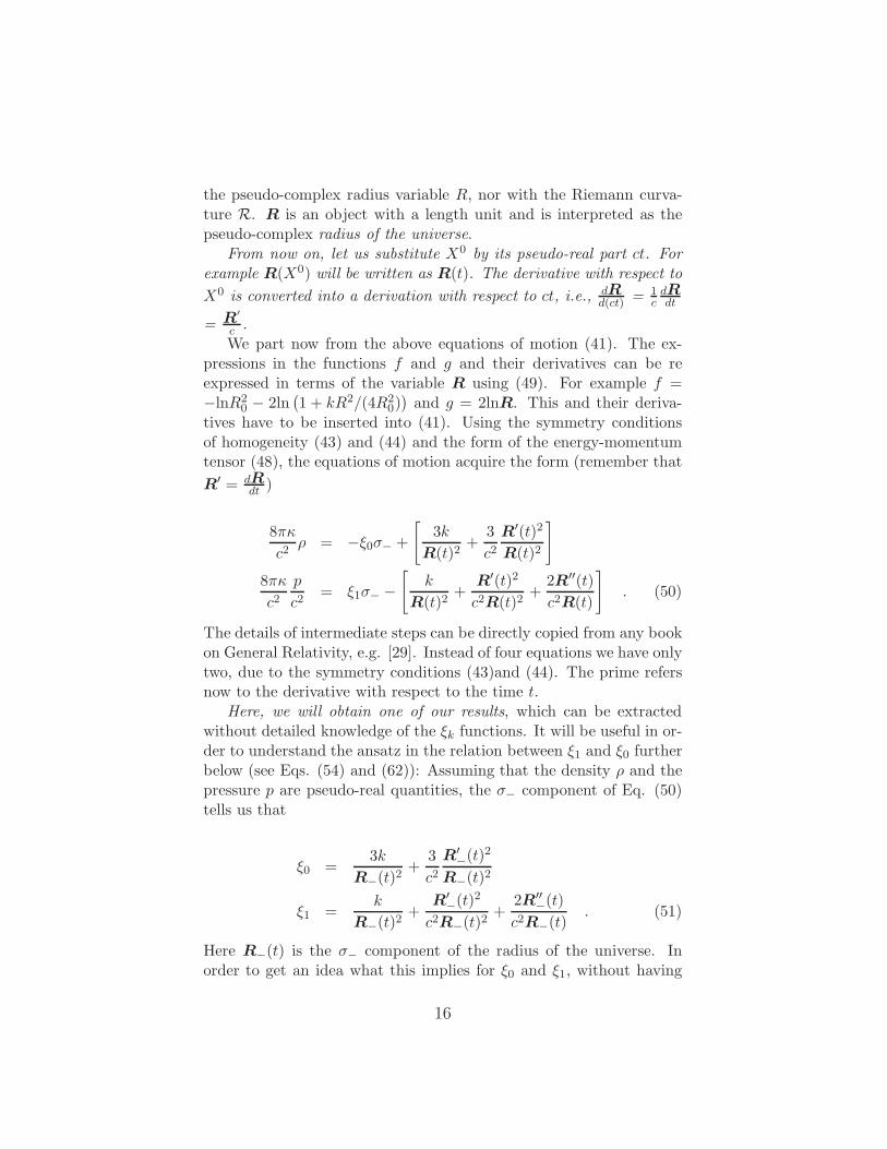
tives have to be inserted into (41). Using the symmetry conditionsof homogeneity (43) and (44) and the form of the energy-momentumtensor (48), the equations of motion acquire the form (remember that

R′ = dR

dt)

8πκ

c2ρ = −ξ0σ− +

[3k

R(t)2+

3

c2R

′(t)2

R(t)2

]

8πκ

c2p

c2= ξ1σ− −

[k

R(t)2+

R′(t)2

c2R(t)2+

2R′′(t)

c2R(t)

]. (50)

The details of intermediate steps can be directly copied from any bookon General Relativity, e.g. [29]. Instead of four equations we have onlytwo, due to the symmetry conditions (43)and (44). The prime refersnow to the derivative with respect to the time t.

Here, we will obtain one of our results, which can be extractedwithout detailed knowledge of the ξk functions. It will be useful in or-der to understand the ansatz in the relation between ξ1 and ξ0 furtherbelow (see Eqs. (54) and (62)): Assuming that the density ρ and thepressure p are pseudo-real quantities, the σ− component of Eq. (50)tells us that

ξ0 =3k

R−(t)2+

3

c2R

′−(t)

2

R−(t)2

ξ1 =k

R−(t)2+

R′−(t)

2

c2R−(t)2+

2R′′−(t)

c2R−(t). (51)

Here R−(t) is the σ− component of the radius of the universe. Inorder to get an idea what this implies for ξ0 and ξ1, without having

16

to solve the problem, we can use the experimental result (Rr is thepseudo-real component of the universe)

R′r

Rr= H with H′ << 1 , (52)

where the prime refers to the derivative with respect to time and H isthe Hubble constant. Because R = Rr + lRI , RI being the pseudo-imaginary component ofR, and l is the length parameter of the theory,which is extremely small (see (I)), we also can assume that R ≈ Rr

and, because RI = 12 (R+ −R−), we can set R± =≈ Rr. Using this

we can approximately write, assuming a nearly constant H = R′

r

Rr,

R′′r

Rr=

R′′r

R′r

R′r

Rr= (lnRr

′)′R

′r

Rr= [ln(HRr)]

′ R′r

Rr

= [lnH + lnRr]′ R

′r

Rr

≈(R

′r

Rr

)2

= H2 . (53)

With that, utilizing (51) and k = 0, we can write the ξ0 and ξ1approximately as

ξ0 ≈ 3

c2H2 ≈ ξ1 . (54)

Further below we will see that this exactly corresponds to the case ofa cosmological constant not changing with the redshift. This wouldbe an exact result, if H is constant all over the history of the universe.Knowing that H is changing in time, implies that there must be adependence on the radius of the universe, i.e., the redshift z. For thatwe have to solve the equation of motion exactly. As we will see furtherbelow, it is not easy to get the exact form of ξ0 and ξ1 but rather theuse of a parametrization is appropriate.

Let us now continue to solve the pc-RW model:

Taking again appropriate linear combinations of (50) (the firstequation of (50) plus three times the second equation of (50) andthe first equation of (50) plus the second one), we get new versions ofthe form

17

4πκ

c2

(ρ+

3p

c2

)=

1

2(3ξ1 − ξ0)σ− − 3R′′

c2R

4πκ

c2

(ρ+

p

c2

)=

1

2(ξ1 − ξ0)σ− +

k

R2 +

R′2 −RR

′′

c2R2 .

(55)

Using that

RR′′ −R

′2

c2R2 =d

dt

(R

′

c2R

), (56)

we arrive at the equation

d

dt

(R

′

c2R

)=

1

2(ξ1 − ξ0)σ− +

k

R2 − 4πκ

c2

(ρ+

p

c2

). (57)

Differentiation of the first equation in (50) with respect to timegives

8πκ

c2dρ

dt= −dξ0

dtσ− − 6k

R3R

′ +6R′

R

d

dt

(1

c2R

′

R

). (58)

Substituting (57) into (58) and multiplying the result by c2

8πκR3, yields

R3 dρ

dt=

c2

8πκ

[−R

3−

dξ0dt

+ 3R2−R

′−(ξ1 − ξ0)

]σ−

−3R2R

′(ρ+p

c2) . (59)

Note that 3R2R

′ = dR3

dt. Shifting the last term of this equation to

the left hand side leads to

d

dt

(ρR3

)+

p

c2dR3

dt=

c2

8πκ

[dR3

−

dt(ξ1 − ξ0)−R

3−

dξ0dt

]σ− .

(60)

18

Identifying the mass within a given volume of the universe byM = ρV ,with V as a given volume, the last equation can be written as

dM

dt+

p

c2dV

dt=

c2

8πκ

[dV−

dt(ξ1 − ξ0)− V−

dξ0dt

]σ− . (61)

This is a local energy balance! In order to maintain local energy con-servation, we have to require that the right hand side is zero. Thisleaves us with the condition

dξ0dt

=d(lnR3

−)

dt(ξ1 − ξ0) . (62)

Any solution for ξ0 and ξ1 has to fulfill this differential equation. Thenegative index of V refers to the fact that the equation holds in the σ−component. Using ξ1 = ξ0 leads to dξ0

dt= 0, or ξ0 = ξ1 = Λ = const.

I.e., for this case we recover the model with a cosmological constantnot changing with time. This equation is not sufficient to solve for ξ0and ξ1; in fact one condition is missing.

The first equation in (55) has the usual interpretation when ξ0 = ξ1= 0. Then the left hand side is the sum of two positive quantities, thedensity and the pressure. The right hand side of (55) is proportionalto the acceleration R

′′ of the radius of the universe, R, multiplied by(-1). This equation tells us that the acceleration of R has to be nega-tive, i.e., we get a de-acceleration. In contrast, in the pseudo-complex

description there is an additional term 12 (3ξ1 − ξ0)σ− present, which

might be positive. Transferring it to the left hand side may give in to-tal a negative function in time, i.e., depending of the functional form

of ξ0 and ξ1 in time, an accelerated phase may be reproduced or not.Let us see whether we can get also acceleration, i.e., that

R′′ > 0 in the pseudo-complex version of GR:Using the left hand side of Eq. (60) (the right hand side is set to

zero as argued below Eq. (61)), we obtain, after multiplying with dt,

R3dρ+ 3R2ρdR +

p

c23R2dR = 0 . (63)

Dividing by 3R3 we obtain

dρ

3+

(ρ+

p

c2

)dR

R= 0 . (64)

19

Finally, dividing by (ρ+ pc2) yields

dρ

3(ρ+ p

c2

) +dR

R= 0 . (65)

Now we have to make an assumption on the equation of state!This is a delicate part and the results can change, depending onwhich equation of state we take. The equation of state may alsodepend on different time epochs. The basic assumptions are that i)the distribution of the mass in the universe can be treated as an idealgas, dust or radiation, the mass being equally distributed (this is onlyapproximately true). The equation of state is

p = αρ , (66)

where ρ is the energy density and α is zero for a model with dust, 23

for a classical ideal gas and 13 for a relativistic ideal gas (radiation).

With this, (65) can be solved with the solution

ρ = ρ0R−3(1+ α

c2) , (67)

where the ρ0 is a pseudo-complex integration constant. Its dimensionis density.

This result is substituted into the first equation of (55), solving forR

′′, yields

R′′ =

c2

6(3ξ1 − ξ0)Rσ− − 4πκ

3(1 +

3α

c2)ρ0R

−(2+ 3αc2

) .

(68)

We will also need the relation

dlnV−

dt=

1

V−

dV−

dt=

1

R3−

d

dtR

3− =

3R′−

R−

=dlnR3

−

dt. (69)

Now we remember our former result that ξ1 has to be approxi-

mately equal to ξ0 (Eq. (54)). Due to this we can assume that thefollowing relation also holds approximately:

20

ξ1 = βξ0 , (70)

where β is an additional parameter of the theory, describing the de-viation from a constant Hubble parameter H. In principle, one canalso use a power expansion of ξ1 in terms of ξ0, which would onlyintroduce more parameters. The β will later be related to observablequantities, like the Hubble constant and the deceleration parameter.Eq. (70) gives us the missing condition, with the prize of having tointroduce an additional parameter. Another possibility is to use theapproximate expression of ξ0 in terms of the ratio (R′

r/Rr), whichgives ξ0 = (3/c2)H, and use experimental observations for H.

Using (62), we obtain for the differential equation for ξ0

dξ0dt

= (β − 1)d(lnR3

−)

dtξ0

=d(lnR

3(β−1)− )

dtξ0 , (71)

with the solution

ξ0 = ΛR3(β−1)− . (72)

This leaves us with the two, yet undetermined, parameters Λ and β.There are many different scenarios:i) β = 1: Then ξ1 = ξ0 = Λ is constant.ii) β 6= 0: This will lead (see further below) to de-accelerated and ac-celerated systems, depending on the value of β. Also the accelerationas a function of the radius of the universe (which can be correlated totime of evolution) depends on β and Λ.

The real part of (68) is obtained by R′′r = 1

2

(R′′

+ +R′′−

). Because

the minimal length scale l is extremely small, we can assume thatR+ ≈ R− ≈ Rr. The real part of (68) is obtained by summing theσ+ and σ− components and dividing the result by 2. We will alsoassume that α+ ≈ α− = α, which is reasonable because the α relatesthe pressure and the density, which are both pseudo-real. Using also(70) and (72) gives the final form of the equation of motion for theradius of the universe

21

R′′r =

c2

12(3β − 1)ΛR3(β−1)+1

r

−4πκ

3(1 +

3α

c2)ρ0R

−3(1+ αc2

)+1r . (73)

We have assumed that the density is real. The first term comes fromthe ξ-functions.

5 Consequences

In this section we shall discuss the consequences of the importantresult (73).

When β = 1 (cosmological constant), the sign of the first termin (73) is positive and contributes to the acceleration of the universe.The acceleration increases with the radius of the universe. For a gen-eral β, the acceleration is positive, as long as β > 1

3 , it is negative(deceleration) for β < 1

3 . For β = 13 no additional acceleration nor

deceleration takes place. The last term in (73) is always negative, i.e.,it represents a contribution which contributes to the deceleration ofthe universe. The behavior of how the accelerating term behaves as afunction in Rr is also determined by β. If the exponent of Rr is pos-itive, the acceleration increases with Rr, if β > 2

3 , while it decreaseswith Rr for β < 2

3 .The solution (73) leaves space for a number of different possible

scenarios. In order to proceed, we will make the following assumption:For simplicity, we assume as before that the parameter α and thedensity ρ0 are pseudo-real, i.e., α+ = α− = α and ρ0+ = ρ0− = ρ. Inthis case the solution simplifies to

R′′r =

c2

12(3β − 1)ΛR3(β−1)+1

r

−4πκ

3(1 +

3α

c2)ρ0R

−3(1+ αc2

)+1r . (74)

With no dark energy, Λ = 0, using (72), we have ξ1 = ξ0 = 0 and thisequation reduces to the one in [29].

Let us now discuss several particular values of β. For that purposewe define

22

Λ =c2

16πκ

Λ

ρ0. (75)

Note that according to (42) the Λ is proportional to ρΛ, the density ofthe dark energy, with the same proportionality factor. Here ρ0 is themass density of the universe. Both densities are of the same order,implying that Λ is of the order of 1.

We can now rewrite (74) into

R′′r =

R′′r(

4πκ3

)ρ0

= Λ (3β − 1)R3(β−1)+1r −

(1 +

3α

c2

)R

−3(1+ αc2

)+1r . (76)

In what follows, we discuss the case of dust dominated universe,i.e., α = 0. For the case of a relativistic ideal gas α = 1

3 , the re-sults show the same characteristics. We will take arbitrarily differentvalues of β, which are chosen such that we will have the case of thecosmological constant Λ, a case which will represent the solution of thebig-rip-off and two new solutions. These solutions are not necessarilyrepresented in nature, i.e., β might have a different intermediate valueas those in the examples. With this we get fora) β = 1: (ξ1 = ξ0 = Λ)

R′′r = 2ΛRr −R

−2r . (77)

The universe is accelerated by the first contribution and deceleratedby the second one. For small Rr the universe is decelerated. For largeRr the first term starts to dominate and the universe is from then onaccelerated. The turning point is at

Rr ≈ 0.79/Λ1

3 . (78)

If we set the radius of today at R0 = 1, a common definition of scalefor the present epoch, the result implies that for Λ = 1 accelerationdid set in after the universe passed 80 percent of its radius. This casecorresponds to a constant cosmological function Λ.

23

b) β = 43 :

R′′r = 3ΛR2

r −R−2r . (79)

In this case, the acceleration increases with the second power in Rr,stronger than only with a cosmological constant. The ξ0 function (72)is then given by ΛR−, i.e., the dark energy density, represented by ξ0,increases with the radius of the universe.. This is like the big rip-off,which is discussed in the literature. The break-even point, i.e. whenacceleration is equal to deceleration, is reached for

Rr = 1/(3Λ)1

4 . (80)

For Λ = 1 the break-even point is reached when the universe is 1/3 ofits present radius, thus, earlier than in case a).c) β = 1

2 : Remember that α = 0 (dust dominated universe)! Then,from (76) we get

R′′r =

1

2ΛR

− 1

2r −R

−2r . (81)

In this situation, the dark energy behaves as (use Eq. (72)) ρ0 =Λ

R3/2r

,

i.e., the density of the dark energy decreases with the radius (time) ofthe universe.

This is really a new solution! The accelerating and the deceleratingparts are decreasing with the size of the universe, but at a different

rate. For small Rr, the second term dominates and the universe isdecelerated, while for sufficient large Rr the first, accelerating, termdominates and the universe is accelerated! The break-even point is at

Rr ≈ 22

3/Λ2

3 , (82)

i.e., for Λ = 1 the universe at this break-even point will be at about2

2

3 ≈ 1.59 times of its present radius. Of course, this can be changedusing different values of Λ. For Λ = 3 the break-even point is at 76percent of the radius of the universe. This case is plotted in figure 1.

24

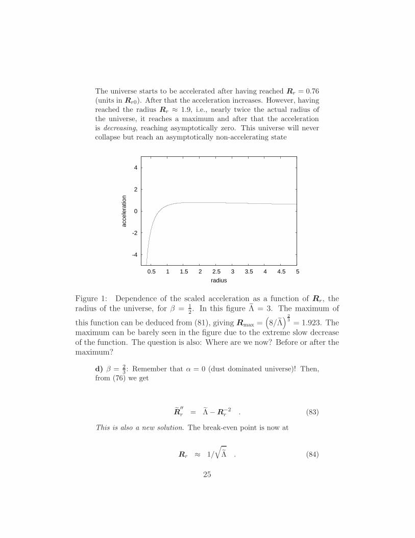
The universe starts to be accelerated after having reached Rr = 0.76(units in Rr0). After that the acceleration increases. However, havingreached the radius Rr ≈ 1.9, i.e., nearly twice the actual radius ofthe universe, it reaches a maximum and after that the accelerationis decreasing, reaching asymptotically zero. This universe will nevercollapse but reach an asymptotically non-accelerating state

-4

-2

0

2

4

0.5 1 1.5 2 2.5 3 3.5 4 4.5 5

acce

lera

tion

radius

Figure 1: Dependence of the scaled acceleration as a function of Rr, theradius of the universe, for β = 1

2. In this figure Λ = 3. The maximum of

this function can be deduced from (81), giving Rmax =(8/Λ

) 2

3 = 1.923. Themaximum can be barely seen in the figure due to the extreme slow decreaseof the function. The question is also: Where are we now? Before or after themaximum?

d) β = 23 : Remember that α = 0 (dust dominated universe)! Then,

from (76) we get

R′′r = Λ−R

−2r . (83)

This is also a new solution. The break-even point is now at

Rr ≈ 1/

√Λ . (84)

25

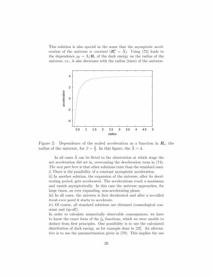
This solution is also special in the sense that the asymptotic accel-eration of the universe is constant (R′′

r = Λ). Using (72) leads tothe dependence ρ0 = Λ/Rr of the dark energy on the radius of theuniverse, i.e., it also decreases with the radius (time) of the universe.

-4

-2

0

2

4

0.5 1 1.5 2 2.5 3 3.5 4 4.5 5

acce

lera

tion

radius

Figure 2: Dependence of the scaled acceleration as a function in Rr, theradius of the universe, for β = 2

3. In this figure, the Λ = 4.

In all cases Λ can be fitted to the observation at which stage thenet acceleration did set in, overcoming the deceleration term in (74).The new part here is that other solutions exist than the standard ones:i) There is the possibility of a constant asymptotic acceleration.ii) In another solution, the expansion of the universe, after its decel-erating period, gets accelerated. The accelerations reach a maximumand vanish asymptotically. In this case the universe approaches, forlarge times, an ever expanding, non-accelerating phase.iii) In all cases, the universe is first decelerated and after a so-calledbreak-even point it starts to accelerate.iv) Of course, all standard solutions are obtained (cosmological con-stant and rip-off).In order to calculate numerically observable consequences, we haveto know the exact form of the ξk functions, which we were unable todeduce from first principles. One possibility is to use the calculateddistribution of dark energy, as for example done in [22]. An alterna-tive is to use the parametrization given in (70). This implies the use

26

of an additional parameter (β) and is equivalent to known consider-ations in the literature [28]. The acceleration in each solution is aconsequence of the ξk functions. As discussed above, they representcontributions to the energy-momentum tensor, equivalent tothe dark energy. In the model considered, this dark energyis in general not a constant but may vary in time, i.e., withthe radius of the universe.

Extraction of β:

We can try to connect the value of β to observable quantities. Forthat, we start from Eq. (53), without the approximation in the lastline. We get

R′′r

Rr

=

[H ′

H+

R′r

Rr

]R

′r

Rr

=

[H ′

H+H

]H = H ′ +H2 . (85)

Substituting this into the expression for ξ1 (Eq. (51)), setting k = 0,we obtain

ξ1 =1

c2H2 +

2

c2

(H ′ +H2

)

=3

c2H2 +

2

c2H ′

= ξ0 +2

c2H ′

= βξ0 , (86)

where we have used that ξ1 = βξ0. Using ξ0 = 3c2H2 (see (54)) and

solving for β, we obtain the final result

β = 1 +2

3

H ′

H2. (87)

We obtained further above that for β > 13 the universe is accel-

erated after a given radius. This corresponds to H′

H2 > −1. In orderto get deeper insight, we use the deceleration parameter, which is ameasure whether the universe is accelerated or decelerated, depending

27

on the sign of this parameter. The deceleration parameter is defined

as [29] q = −R′′

rRr

R′2

r

, which gives q = −[1 + H′

H2

]. The universe is

accelerated when β < 13 , or

H′

H2 < −1, or q > 0. The acceleration

increases with Rr when β > 23 , or

H′

H2 > −12 , or q < −1

2 .In conclusion, a measurement of the change of the Hubble constant

with time will lead to a determination of the parameter β as a functionof time. Though, the last considerations clarify the role of β, we aresuffering still by the problem that we have to know the solution of

H = R′

r

Rr. This can be done up to now only through the experimental

measurement of the Hubble parameter H.

A model including dust and radiation, k=0:

Up to now, we did only consider one density component (dustor radiation) and the pseudo-complex contribution, given by the ξkfunctions. Realistic models involve both components, as can be seenin [28]. Expressing the ratio of the radii Rr0 and Rr, the presentradius of the universe and the one at a redshift z, respectively, interms of the redshift, we obtain [29, 28]

Rr0

Rr= (1 + z) , (88)

where the index r refers to the real value of the radius. We obtain forthe ratio of the velocity and the the radius of the universe [28]

R′r

Rr= H = H2

0

Ωd(1 + z)3 +Ωr(1 + z)4 +ΩΛf(z)

(89)

where the index d refers to the dust part and the index r to theradiation part. We do not include the contribution due to k 6= 0,because we consider a flat universe. The factor H2

0 is the square ofthe present Hubble constant. Using our previous result, the functionf(z) is given by

f(z) = (1 + z)3(β−1) = (1 + z)3(1+w) , (90)

(β = 2+w) where we made a connection to the notation used in [28].Our result states that when the Hubble constant changes in time,

28

there must be a deviation from β = 1, which corresponds to w = −1,the case of a cosmological constant, constant in time. The deviationfrom β = 1 cannot be large whenH ′, the time derivative of the Hubbleconstant, is small. Up to now, we only find a parametrization of the ξkfunctions in terms of the Hubble parameter or the parameter β. Thedeeper origin of the value of ξk can probably explained by fundamentaltheories like string theories.

Note, that the relation β = 2+w with (87) gives a relation of w tothe Hubble parameter and its derivative in time, which makes definitepredictions on w, once H and H ′ are known. To our knowledge, thisis not presented elsewhere.

6 Conclusions

We have applied the pseudo-complex formalism to extend the Robertson-Walker model of the universe to the pc-RW model. The main resultsare that1) The model introduces automatically a contribution which is equalto the cosmological constant or dark energy which may depend on theradius of the universe.2) The cosmological ”constant” is a constant when the Hubble con-stant is constant too. When the Hubble constant changes slightly withtime, our model predicts deviations from the cosmological constant,depending on the redshift (time of expansion). The amount of devia-tions depends on the exact form of the ξk functions.3) The deviation can be obtained, once the radius of the universe, asa function of time, is known. Within our theory, we obtain severalpossible dependencies of the dark energy as a function in the radiusof the universe, depending on the parameter β.4) We also obtained several possible evolutions of the universe. Be-sides the solution of a constant dark energy density and the rip-offscenario, we also obtained solutions where the acceleration tends forinfinite time towards zero or a constant value (see Figs. 1 and 2).5) We obtained a relation between w = β− 2 and H and H ′. Once Hand H ′ are known, the w value can be deduced.

The origin of the ξk functions might have a deeper microscopicorigin, which we do not explore here. Probably, only such a deepermicroscopic understanding will fix the dependence of ξk on the ra-dius of the universe (see for example [22]). Nevertheless, the classical

29

picture presented here enlightens and simplifies the description of dif-ferent possible evolution scenarios of the universe.

We have not yet investigated the role of the minimal length param-eter l, which also appears in the pseudo-complex formulation. In fieldtheory its function is to render the theory regularized [30]. We suspectthat this also happens in the pseudo-complex formulation of GeneralRelativity and might give a hint on how to quantize this theory. Ina future publication we intend to investigate the role of the minimallength scale l.

We saw that the modified variational principle δS ǫ P0 has impor-tant consequences as the appearance of dark energy. It also providesa simpler description of effects of the dark energy, obtained via quiteinvolved numerical calculations, as for example in [22]. These featuresare a hint that the variational principle has to be probably modifiedas proposed.

Acknowledgments

P.O.H. wants to express sincere gratitude for the possibility to workat the Frankfurt Institute of Advanced Studies and of the excellentworking atmosphere encountered there. He also acknowledges finan-cial support from DGAPA and CONACyT.

References

[1] A. Einstein, Ann. Math. 46, 578 (1945).

[2] A. Einstein, Rev. Mod. Phys. 20. 35 (1948).

[3] C. Mantz and T. Prokopec, arXiv:gr-qc—0804.0213v1, 2008.

[4] D. Lovelook, Annali di Matematica Pura 83, No. 1 (1969), 43.

[5] E. R. Caianiello, Nuovo Cim. Lett. 32, 65 (1981).

[6] H. E. Brandt, Found. Phys. Lett. 2, 39 (1989).

[7] H. E. Brandt, Found. Phys. Lett. 4, 523 (1989).

[8] H. E. Brandt, Found. Phys. Lett. 6, 245 (1993).

[9] R. G. Beil, Found. Phys. 33, 1107 (2003).

[10] R. G. Beil, Int. J. Theor. Phys. 26, 189 (1987).

[11] R. G. Beil, Int. J. Theor. Phys. 28, 659 (1989).

30

[12] R. G. Beil, Int. J. Theor. Phys. 31, 1025 (1992).

[13] J. W. Moffat, Phys. Rev. D 19, 3554 (1979).

[14] G. Kunstatter, J. W. Moffat and J. Malzan, J. Math. Phys. 24,886 (1983).

[15] G. Kunstatter and R. Yates, J. Phys. A 14, 847 (1981).

[16] A. Crumeyrolle, Ann. de la Fac. des Sciences de Toulouse, 4e

serie, 26, 105 (1962).

[17] A. Crumeyrolle, Riv. Mat. Univ. Parma (2) 5, 85 (1964).

[18] R.-L. Clerc, Ann. de L’I.H.P. Section A 12, No. 4, 343 (1970).

[19] R.-L. Clerc, Ann. de L’I.H.P. Section A 17, No. 3, 227 (1972).

[20] P. O.Hess and W. Greiner, Int. J. Mod. Phys. E 18 (2009), 51.

[21] C. W. Misner, K. S. Thorne, J. A. Wheeler, Gravitation, (W. H.Freeman Company, San Francisco, 1973)

[22] J. A. Gonzalez and F. S. Guzman, Phys. Rev. D 79 (2009),121501.

[23] A. Feoli, G. Lambiase, G. Papini and G. Scarpetta, Phys. Lett A263 (1999), 147.

[24] P. O. Hess and W. Greiner, JPG (2007).

[25] P. O. Hess and W. Greiner, Int. J. Mod. Phys. E (2007).

[26] I. L. Kantor, A. S. Solodovnikov, Hypercomplex Numbers. An

Elementary Introduction to Algebra, (Springer, Heidelberg,1989).

[27] V. Cruceanu, P. Fortuny and P. M. Gadea, Rocky Mountain J.

of Math. 26, 83 (1996).

[28] P. J. E. Peebles, Rev. Mod. Phys. 75 (2003), 559.

[29] R. Adler, M. Bazin and M. Schiffer, Introduction to General Rel-

ativity, (McGraw Hill, New York, 1975).

[30] P. O. Hess and W. Greiner, Int. J. Mod. Phys. E 16 (2007), 1643.

31