Thermodynamics of Glaciers of Glaciers ... 1. ThermodynamicsofGlaciers ... Canadian-type glaciers are mostly cold 10. ThermodynamicsofGlaciers

Thermodynamics of Glaciers

McCarthy Summer School 2012

Andy AschwandenUniversity of Alaska Fairbanks, USA

June 2012

Note: This script is largely based on the Physics of Glaciers I lecture notes by MartinLüthi and Martin Funk, ETH Zurich, Switzerland, with additions from Greve and Blatter(2009) and Gusmeroli et al. (2010).

Glaciers are divided into three categories, depending on their thermal structure

Cold The temperature of the ice is below the pressure melting temperature throughoutthe glacier, except for maybe a thin surface layer.

Temperate The whole glacier is at the pressure melting temperature, except for seasonalfreezing of the surface layer.

Polythermal Some parts of the glacier are cold, some temperate. Usually the highestaccumulation area, as well as the upper part of an ice column are cold, whereas thesurface and the base are at melting temperature.

The knowledge of the distribution of temperature in glaciers and ice sheets is of highpractical interest

• A temperature profile from a cold glacier contains information on past climateconditions.

• Ice deformation is strongly dependent on temperature (temperature dependence ofthe rate factor A in Glen’s flow law).

• The routing of meltwater through a glacier is affected by ice temperature. Cold iceis essentially impermeable, except for discrete cracks and channels.

• If the temperature at the ice-bed contact is at the pressure melting temperaturethe glacier can slide over the base.

1


• Wave velocities of radio and seismic signals are temperature dependent. This affectsthe interpretation of ice depth soundings.

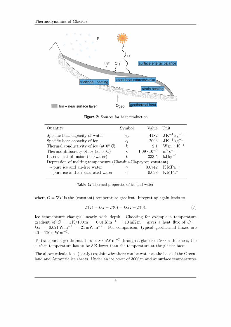
The distribution of temperature in a glacier depends on many factors. Heat sourcesare on the glacier surface, at the glacier base and within the body of the ice. Heat istransported through a glacier by conduction (diffusion), is advected with the moving ice,and is convected with water or air flowing through cracks and channels. Heat sourceswithin the ice body are (Figure 2)

• dissipative heat production (internal friction) due to ice deformation,

• frictional heating at the glacier base (basal motion)

• frictional heating of flowing water at englacial channel walls,

• release or consumption of (latent) heat due to freezing and melting.

The importance of the processes depends on the climate regime a glacier is subjected to,and also varies between different parts of the same glacier.

1 Energy balance equation

The energy balance equation in the form suitable to calculate ice temperature within aglacier is the advection-diffusion equation which in a spatially fixed (Eulerian) referenceframe is given by

ρ c

(∂T

∂t+ v∇T

)= ∇(k∇T ) + P . (1)︸︷︷︸

advection︸︷︷︸diffusion

︸︷︷︸production

The ice temperature T (x, t) at location x and time t changes due to advection, diffusionand production of heat. The material constants density ρ, specific heat capacity c andthermal conductivity k are given in Table 1. In general, specific heat capacity and thermalheat conductivity are functions of temperature (e.g. Ritz , 1987),

c(T ) = (146.3 + 7.253T [K]) J kg−1 K−1 (2)

andk(T ) = 9.828e−0.0057T [K] Wm−1 K−1. (3)

For constant thermal conductivity k and in one dimension (the vertical direction z andvertical velocity w) the energy balance equation (1) reduces to

ρ c

(∂T

∂t+ w

∂T

∂z

)= k

∂2T

∂z2+ P. (4)

The heat production (source term) P can be due to different processes (see Figure 2):

2


−50 −40 −30 −20 −10 0

2.2

2.4

2.6

temperature θ [° C]

k [W

m−

1 K−

1 ]

−50 −40 −30 −20 −10 0

1800

1900

2000

2100

temperature θ [° C]

c [J

kg−

1 K−

1 ]

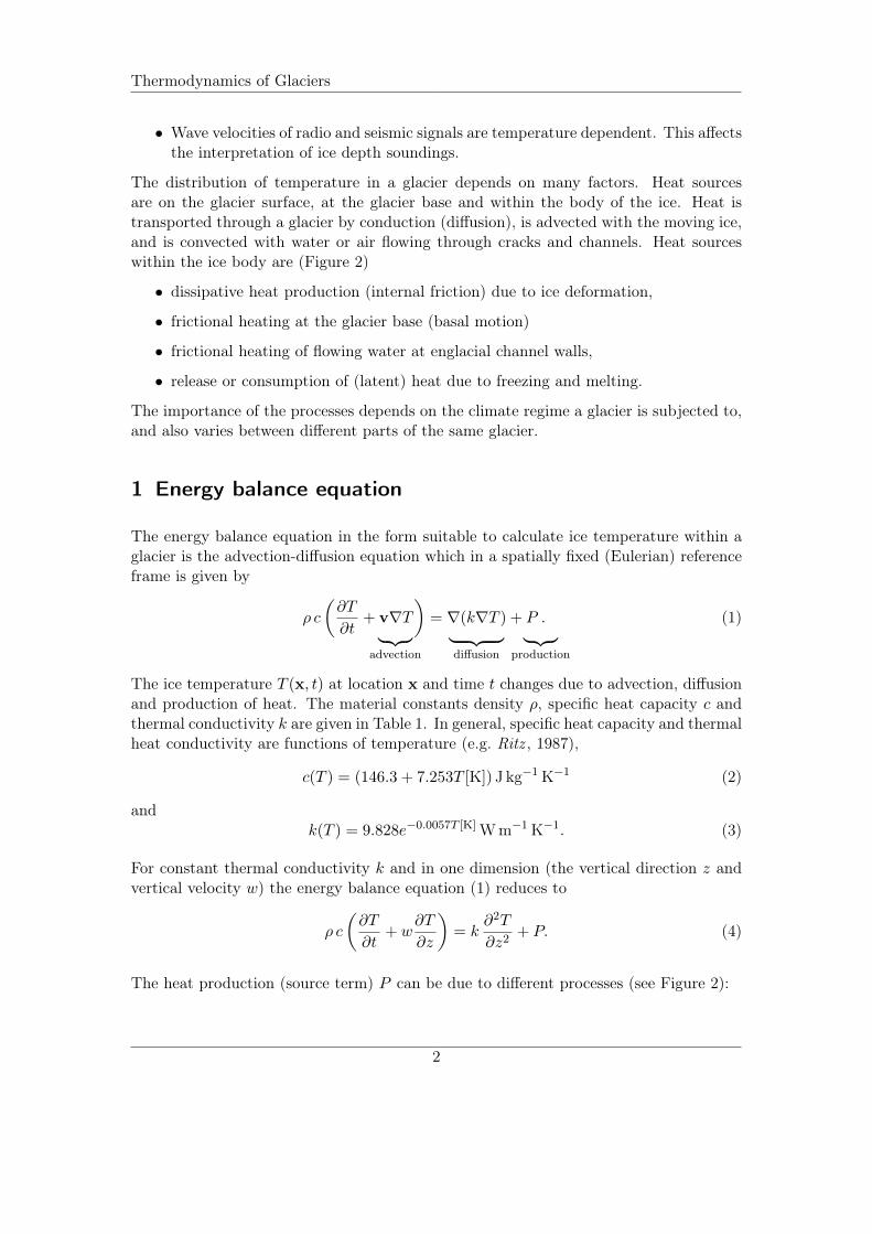
Figure 1: Heat conductivity k (left) and specific heat c (right) for the temperature range from−50◦ C until 0◦ C. After Ritz (1987).

Dissipation In viscous flow the dissipation due to ice deformation (heat release due tointernal friction, often called strain heating) is P = tr(εσ) = εijσji, where ε andσ are the strain rate tensor and the stress tensor, respecitively.. Because usuallythe shearing deformation dominates glacier flow

Pdef ' 2 εxzσxz .

Sliding friction The heat production is the rate of loss of potential energy as an icecolumn of thickness H moves down slope. If all the frictional energy is released atthe bed due to sliding with basal velocity ub,

Pfriction = τbub ∼ ρgH tanβ ub ,

where τb is basal shear stress and β is the bed inclination.

Refreezing of meltwater Consider ice that contains a volume fraction ω of water. If afreezing front is moving with a velocity vfreeze relative to the ice, the rate of latentheat production per unit area of the freezing front is

Pfreeze = vfreeze ωρwL.

2 Steady temperature profile

The simplest case is a vertical steady state temperature profile (Eq. 4 without timederivative) in stagnant ice (w = 0) without any heat sources (P = 0), and with con-stant thermal conductivity k. The heat flow equation (4) then reduces to the diffusionequation

∂2T

∂z2= 0. (5)

Integration with respect to z gives

dT

dz= Q := kG (6)

3


QE QH

R

Qgeo

P

surface energy balance

strain heating

fricitional heating

geothermal heatfirn + near surface layer

latent heat sources/sinks

Figure 2: Sources for heat production

Quantity Symbol Value Unit

Specific heat capacity of water cw 4182 J K−1 kg−1

Specific heat capacity of ice ci 2093 J K−1 kg−1

Thermal conductivity of ice (at 0◦C) k 2.1 W m−1 K−1

Thermal diffusivity of ice (at 0◦C) κ 1.09 · 10−6 m2 s−1

Latent heat of fusion (ice/water) L 333.5 kJ kg−1

Depression of melting temperature (Clausius-Clapeyron constant)- pure ice and air-free water γ 0.0742 K MPa−1

- pure ice and air-saturated water γ 0.098 K MPa−1

Table 1: Thermal properties of ice and water.

where G = ∇T is the (constant) temperature gradient. Integrating again leads to

T (z) = Qz + T (0) = kGz + T (0). (7)

Ice temperature changes linearly with depth. Choosing for example a temperaturegradient of G = 1 K/100 m = 0.01 K m−1 = 10 mK m−1 gives a heat flux of Q =kG = 0.021 W m−2 = 21 mW m−2. For comparison, typical geothermal fluxes are40− 120 mW m−2.

To transport a geothermal flux of 80 mW m−2 through a glacier of 200 m thickness, thesurface temperature has to be 8 K lower than the temperature at the glacier base.

The above calculations (partly) explain why there can be water at the base of the Green-land and Antarctic ice sheets. Under an ice cover of 3000 m and at surface temperatures

4


of −50◦C (in Antarctica), only a heat flux of Q = k · 50 K/3000 m = 35 mW m−2 canbe transported away. Notice that horizontal and vertical advection change this resultconsiderably.

3 Ice temperature close to the glacier surface

The top 15 m of a glacier (near surface layer, Figure 2) are subject to seasonal variationsof temperature. In this part of the glacier heat flow (heat diffusion) is dominant. If weneglect advection we can rewrite Equation (4) to obtain the well known Fourier law ofheat diffusion

∂T

∂t= κ

∂2T

∂h2(8)

where h is depth below the surface, and κ = k/(ρC) is the thermal diffusivity of ice.To calculate a temperature profile and changes with time we need boundary conditions.Periodically changing boundary conditions at the surface such as day/night and win-ter/summer can be approximated with a sine function. At depth we assume a constanttemperature T0

T (0, t) = T0 + ∆T0 · sin(ωt) ,

T (∞, t) = T0 . (9)

T0 is the mean surface temperature and ∆T0 is the amplitude of the periodic changes ofthe surface temperature. The duration of a period is 2π/ω. The solution of Equation (8)with the boundary condition (9) is

T (h, t) = T0 + ∆T0 exp

(−h√

ω

2κ

)sin

(ωt− h

√ω

2κ

). (10)

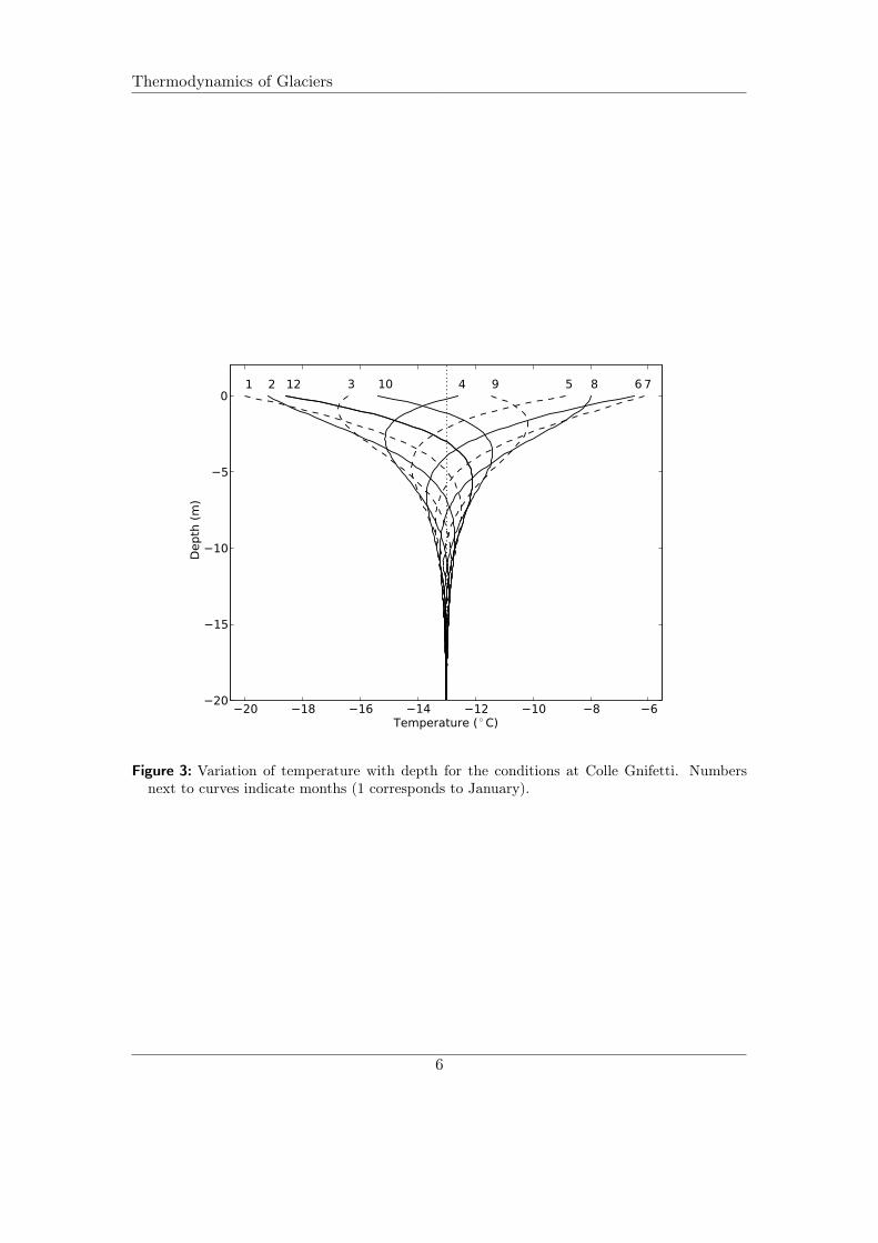
The solution is plotted for realistic values of T0 and ∆T on Colle Gnifetti (4550 m a.s.l.,Monte Rosa, Valais). Notice that full ice density has been assumed for the plot, instead ofa firn layer with strongly changing thermal properties, and vertical advection is neglected.

The solution (Eq. 10) has some noteworthy properties

a) The amplitude varies with depth h as

∆T (h) = ∆T0 exp

(−h√

ω

2κ

)(11)

b) The temperature T (h, t) has an extremum when

sin

(ωt− h

√ω

2κ

)= ±1 ⇒ ωt− h

√ω

2κ=π

2

5


20 18 16 14 12 10 8 6Temperature ( ◦ C)

20

15

10

5

0

Depth

(m

)

1 2 3 4 5 6 7891012

Figure 3: Variation of temperature with depth for the conditions at Colle Gnifetti. Numbersnext to curves indicate months (1 corresponds to January).

6


and therefore

tmax =1

ω

(π

2+ h

√ω

2κ

)(12)

The phase shift is increasing with depth below the surface.

c) The heat flux G(h, t) in a certain depth h below the surface is

G(h, t) = −k∂T∂h

= (complicated formula that is easy to derive)

For the heat flux G(0, t) at the glacier surface we get

G(0, t) = ∆T0

√ωρ c k sin

(ωt+

π

4

)G(0, t) is maximal when

sin(ωt+

π

4

)= 1 ⇒ ωt+

π

4=π

2=⇒ tmax =

π

4ω

where tmax is the time when the heat flux at the glacier surface is maximum.

Temperature: tmax =π

2ω

Heat flux: tmax =π

4ω

The difference is π/(4ω) and thus 1/8 of the period. The maximum heat flux atthe glacier surface is 1/8 of the period ahead of the maximum temperature. For ayearly cycle this corresponds to 1.5 months.

d) From the ratio between the amplitudes in two different depths the heat diffusivityκ can be calculated

∆T2

∆T1= exp

((h1 − h2)

√ω

2κ

)=⇒ κ =

ω

2

(h2 − h1

ln ∆T2∆T1

)2

There are, however, some restrictions to the idealized picture given above

• The surface layers are often not homogeneous. In the accumulation area densityis increasing with depth. Conductivity k and diffusivity κ are functions of density(and also temperature).

• In nature the surface boundary condition is not a perfect sine function.

• The ice is moving. Heat diffusion is only one part, heat advection may be equallyimportant.

• Percolating and refreezing melt water can drastically change the picture by provid-ing a source of latent heat (see below).

7


Superimposed on the yearly cycle are long term temperature changes at the glacier sur-face. These penetrate much deeper into the ice, as can be seen from Equation (11), sinceω decreases for increasing forcing periods.

In spring or in high accumulation areas the surface layer of a glacier consists of snow orfirn. If surface melting takes place, the water percolates into the snow or firn pack andfreezes when it reaches a cold layer. The freezing of 1 g of water releases sufficient heat toraise the temperature of 160 g of snow by 1 K. This process is important to “annihilate”the winter cold from the snow or firn cover in spring, and is the most important processaltering the thermal structure of high accumulation areas and of the polar ice sheets.

4 Temperate glaciers

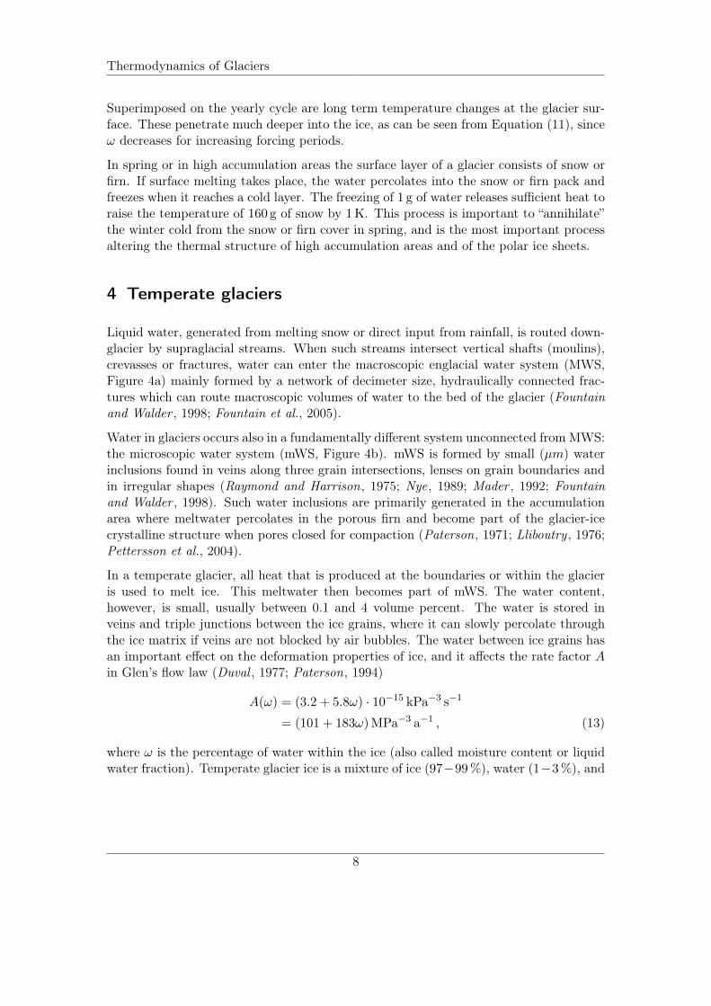
Liquid water, generated from melting snow or direct input from rainfall, is routed down-glacier by supraglacial streams. When such streams intersect vertical shafts (moulins),crevasses or fractures, water can enter the macroscopic englacial water system (MWS,Figure 4a) mainly formed by a network of decimeter size, hydraulically connected frac-tures which can route macroscopic volumes of water to the bed of the glacier (Fountainand Walder , 1998; Fountain et al., 2005).

Water in glaciers occurs also in a fundamentally different system unconnected from MWS:the microscopic water system (mWS, Figure 4b). mWS is formed by small (µm) waterinclusions found in veins along three grain intersections, lenses on grain boundaries andin irregular shapes (Raymond and Harrison, 1975; Nye, 1989; Mader , 1992; Fountainand Walder , 1998). Such water inclusions are primarily generated in the accumulationarea where meltwater percolates in the porous firn and become part of the glacier-icecrystalline structure when pores closed for compaction (Paterson, 1971; Lliboutry , 1976;Pettersson et al., 2004).

In a temperate glacier, all heat that is produced at the boundaries or within the glacieris used to melt ice. This meltwater then becomes part of mWS. The water content,however, is small, usually between 0.1 and 4 volume percent. The water is stored inveins and triple junctions between the ice grains, where it can slowly percolate throughthe ice matrix if veins are not blocked by air bubbles. The water between ice grains hasan important effect on the deformation properties of ice, and it affects the rate factor Ain Glen’s flow law (Duval , 1977; Paterson, 1994)

A(ω) = (3.2 + 5.8ω) · 10−15 kPa−3 s−1

= (101 + 183ω) MPa−3 a−1 , (13)

where ω is the percentage of water within the ice (also called moisture content or liquidwater fraction). Temperate glacier ice is a mixture of ice (97−99 %), water (1−3 %), and

8


small amounts of air and minerals. For pure ice the melting temperature Tm depends onabsolute pressure p by

Tm = Ttp − γ (p− ptp) , (14)

where Ttp = 273.16 K and ptp = 611.73 Pa are the triple point temperature and pressureof water. The Clausius-Clapeyron constant is γp = 7.42·10−5 K kPa−1 for pure water/ice.Since glacier ice is not pure, the value of γ can be as high as γa = 9.8 · 10−5 K kPa−1 forair saturated water (Harrison, 1975).

. .. .. .. .. .. .. . .. .. .. . ... . . . ...

bedrocktemperate ice

firncold ice

. ... . mWS microscoptic water systemMWS macroscoptic water system

mWS

waterinclusionb

temperate ice

cold-dry icecWS

C SMT

a

Figure 4: Illustration of macroscopic water system (MWS) and microscopic water system (mWS)found in the temperate ice. The cold-temperate transition surface (CTS) is the englacialboundary separating temperate ice (b) from the cold ice (c). Modified after Gusmeroli et al.(2010)

5 Cold glaciers

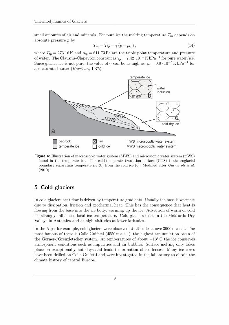
In cold glaciers heat flow is driven by temperature gradients. Usually the base is warmestdue to dissipation, friction and geothermal heat. This has the consequence that heat isflowing from the base into the ice body, warming up the ice. Advection of warm or coldice strongly influences local ice temperature. Cold glaciers exist in the McMurdo DryValleys in Antartica and at high altitudes at lower latitudes.

In the Alps, for example, cold glaciers were observed at altitudes above 3900 m a.s.l.. Themost famous of these is Colle Gnifetti (4550 m a.s.l.), the highest accumulation basin ofthe Gorner-/Grenzletscher system. At temperatures of about −13◦C the ice conservesatmospheric conditions such as impurities and air bubbles. Surface melting only takesplace on exceptionally hot days and leads to formation of ice lenses. Many ice coreshave been drilled on Colle Gnifetti and were investigated in the laboratory to obtain theclimate history of central Europe.

9


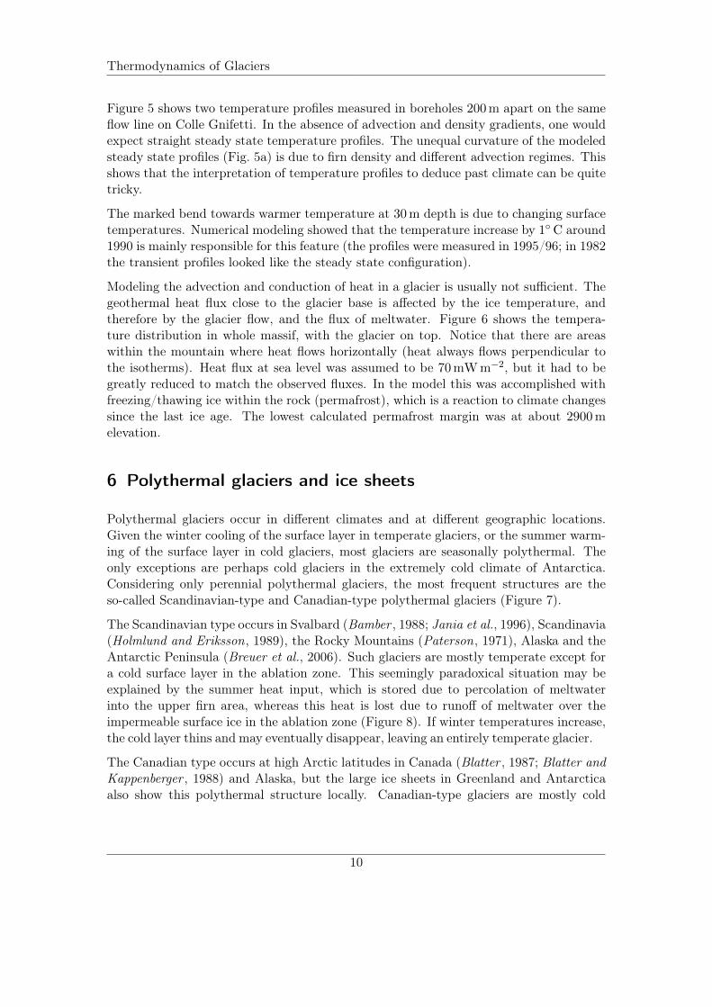
Figure 5 shows two temperature profiles measured in boreholes 200 m apart on the sameflow line on Colle Gnifetti. In the absence of advection and density gradients, one wouldexpect straight steady state temperature profiles. The unequal curvature of the modeledsteady state profiles (Fig. 5a) is due to firn density and different advection regimes. Thisshows that the interpretation of temperature profiles to deduce past climate can be quitetricky.

The marked bend towards warmer temperature at 30 m depth is due to changing surfacetemperatures. Numerical modeling showed that the temperature increase by 1◦C around1990 is mainly responsible for this feature (the profiles were measured in 1995/96; in 1982the transient profiles looked like the steady state configuration).

Modeling the advection and conduction of heat in a glacier is usually not sufficient. Thegeothermal heat flux close to the glacier base is affected by the ice temperature, andtherefore by the glacier flow, and the flux of meltwater. Figure 6 shows the tempera-ture distribution in whole massif, with the glacier on top. Notice that there are areaswithin the mountain where heat flows horizontally (heat always flows perpendicular tothe isotherms). Heat flux at sea level was assumed to be 70 mW m−2, but it had to begreatly reduced to match the observed fluxes. In the model this was accomplished withfreezing/thawing ice within the rock (permafrost), which is a reaction to climate changessince the last ice age. The lowest calculated permafrost margin was at about 2900 melevation.

6 Polythermal glaciers and ice sheets

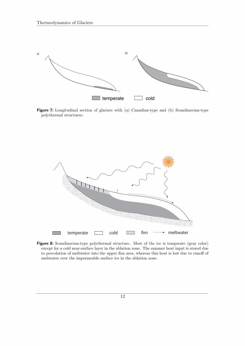
Polythermal glaciers occur in different climates and at different geographic locations.Given the winter cooling of the surface layer in temperate glaciers, or the summer warm-ing of the surface layer in cold glaciers, most glaciers are seasonally polythermal. Theonly exceptions are perhaps cold glaciers in the extremely cold climate of Antarctica.Considering only perennial polythermal glaciers, the most frequent structures are theso-called Scandinavian-type and Canadian-type polythermal glaciers (Figure 7).

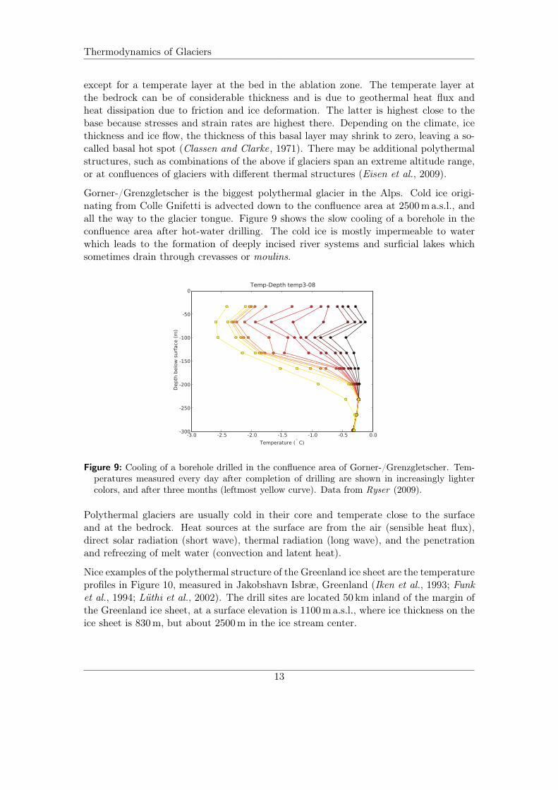
The Scandinavian type occurs in Svalbard (Bamber , 1988; Jania et al., 1996), Scandinavia(Holmlund and Eriksson, 1989), the Rocky Mountains (Paterson, 1971), Alaska and theAntarctic Peninsula (Breuer et al., 2006). Such glaciers are mostly temperate except fora cold surface layer in the ablation zone. This seemingly paradoxical situation may beexplained by the summer heat input, which is stored due to percolation of meltwaterinto the upper firn area, whereas this heat is lost due to runoff of meltwater over theimpermeable surface ice in the ablation zone (Figure 8). If winter temperatures increase,the cold layer thins and may eventually disappear, leaving an entirely temperate glacier.

The Canadian type occurs at high Arctic latitudes in Canada (Blatter , 1987; Blatter andKappenberger , 1988) and Alaska, but the large ice sheets in Greenland and Antarcticaalso show this polythermal structure locally. Canadian-type glaciers are mostly cold

10


-14.0 -13.5 -13.0 -12.5 -12.0Temperature [oC]

-100

-80

-60

-40

-20

0

Dep

th b

elow

sur

face

[m]

B 95-2

B 95-1

Q=0 mW/m2

steady stateTsurf = -14.0oC var.

-14.0 -13.5 -13.0 -12.5 -12.0Temperature [oC]

-100

-80

-60

-40

-20

0

Dep

th b

elow

sur

face

[m]

B 95-2

B 95-1

Figure 5: Markers indicate temperatures measured in two boreholes on the same flow line, 200 mapart, on Colle Gnifetti. Solid lines are the results of numerical interpretation of the datawith steady state (left) and transient (right) temperature evolution. Notice that the differentcurvature of the steady state profiles is due to firn density and advection. From Lüthi andFunk (2001).

0 500 1000 1500Distance along flowline [m]

3000

3500

4000

4500

Altit

ude

[m a

.s.l]

Tsurf(t)

3 322

1 1

-1-1

-2-2-3

-3

-4

-4

-5

-5

-6

-7

-8

-9

-10

-12

-13

-11

q

0 200 400 600 800Distance along flowline [m]

3800

4000

4200

4400

4600

Altit

ude

[m a

.s.l]

-5

-6

-6

-7

-7

-8

-8

-9

-9

-12

-12

-11

-11-1

0

-10

-13

-13

-6

Figure 6: Modeled temperature distribution within the Monte Rosa massif. Notice the highlyincreased surface temperature on the south (right) face which leads to horizontal heat fluxesclose to steep mountain faces. Thawing permafrost at the base of the mountain was essentialto reproduce the measured heat flux at the glacier base. From Lüthi and Funk (2001).

11


temperate cold

a) b)

Figure 7: Longitudinal section of glaciers with (a) Canadian-type and (b) Scandinavian-typepolythermal structures.

temperate cold firn meltwater

Figure 8: Scandinavian-type polythermal structure. Most of the ice is temperate (gray color)except for a cold near-surface layer in the ablation zone. The summer heat input is stored dueto percolation of meltwater into the upper firn area, whereas this heat is lost due to runoff ofmeltwater over the impermeable surface ice in the ablation zone.

12


except for a temperate layer at the bed in the ablation zone. The temperate layer atthe bedrock can be of considerable thickness and is due to geothermal heat flux andheat dissipation due to friction and ice deformation. The latter is highest close to thebase because stresses and strain rates are highest there. Depending on the climate, icethickness and ice flow, the thickness of this basal layer may shrink to zero, leaving a so-called basal hot spot (Classen and Clarke, 1971). There may be additional polythermalstructures, such as combinations of the above if glaciers span an extreme altitude range,or at confluences of glaciers with different thermal structures (Eisen et al., 2009).

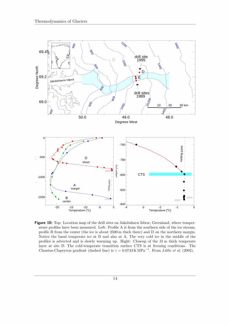
Gorner-/Grenzgletscher is the biggest polythermal glacier in the Alps. Cold ice origi-nating from Colle Gnifetti is advected down to the confluence area at 2500 m a.s.l., andall the way to the glacier tongue. Figure 9 shows the slow cooling of a borehole in theconfluence area after hot-water drilling. The cold ice is mostly impermeable to waterwhich leads to the formation of deeply incised river systems and surficial lakes whichsometimes drain through crevasses or moulins.

Figure 9: Cooling of a borehole drilled in the confluence area of Gorner-/Grenzgletscher. Tem-peratures measured every day after completion of drilling are shown in increasingly lightercolors, and after three months (leftmost yellow curve). Data from Ryser (2009).

Polythermal glaciers are usually cold in their core and temperate close to the surfaceand at the bedrock. Heat sources at the surface are from the air (sensible heat flux),direct solar radiation (short wave), thermal radiation (long wave), and the penetrationand refreezing of melt water (convection and latent heat).

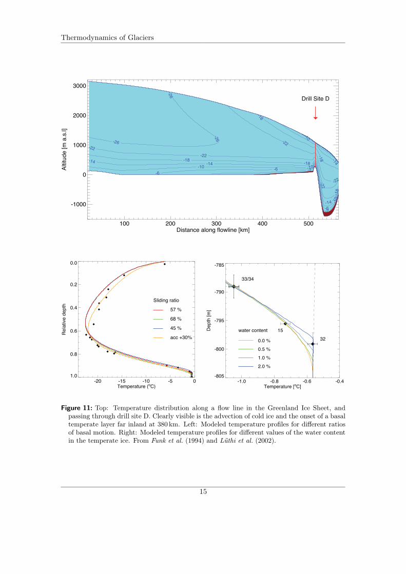
Nice examples of the polythermal structure of the Greenland ice sheet are the temperatureprofiles in Figure 10, measured in Jakobshavn Isbræ, Greenland (Iken et al., 1993; Funket al., 1994; Lüthi et al., 2002). The drill sites are located 50 km inland of the margin ofthe Greenland ice sheet, at a surface elevation is 1100 m a.s.l., where ice thickness on theice sheet is 830 m, but about 2500 m in the ice stream center.

13


50.0 49.0 48.0Degrees West

69.0

69.2

69.4

Deg

rees

Nor

th

0 10 20 30 km

400

400

400

400

400

600

600

800

800

1000

1000

1200

1200

1400

1400

1600

ED

drill sites 1989

drill site 1995

Jakobshavns Isfjord

-20 -15 -10 -5 0Temperature (oC)

-1500

-1000

-500

0

Dep

th b

elow

sur

face

(m

)

Dsheet

Amargin

Bcenter

mel

ting

poin

t

-4 -3 -2 -1 0Temperature [oC]

-840

-820

-800

-780

-760

Dep

th [m

]

CTS

mel

ting

poin

t

Figure 10: Top: Location map of the drill sites on Jakobshavn Isbræ, Greenland, where temper-ature profiles have been measured. Left: Profile A is from the southern side of the ice stream,profile B from the center (the ice is about 2500 m thick there) and D on the northern margin.Notice the basal temperate ice at D and also at A. The very cold ice in the middle of theprofiles is advected and is slowly warming up. Right: Closeup of the 31 m thick temperatelayer at site D. The cold-temperate transition surface CTS is at freezing conditions. TheClausius-Clapeyron gradient (dashed line) is γ = 0.0743 K MPa−1. From Lüthi et al. (2002).

14


100 200 300 400 500Distance along flowline [km]

-1000

0

1000

2000

3000

Altit

ude

[m a

.s.l]

-6-6

-6

-10

-10-10-14 -14

-14

-18

-18-18

-22-22

-22

-22

-22-18

-18 -14

-10

-2

-2

-26

-26-26

Drill Site D

-20 -15 -10 -5 0Temperature (oC)

1.0

0.8

0.6

0.4

0.2

0.0

Rel

ativ

e de

pth

Sliding ratio

68 %

45 %

acc +30%

57 %

-1.0 -0.8 -0.6 -0.4Temperature [oC]

-805

-800

-795

-790

-785

Dep

th [m

]

0.0 %0.5 %1.0 %2.0 %

3215

33/34

water content

Figure 11: Top: Temperature distribution along a flow line in the Greenland Ice Sheet, andpassing through drill site D. Clearly visible is the advection of cold ice and the onset of a basaltemperate layer far inland at 380 km. Left: Modeled temperature profiles for different ratiosof basal motion. Right: Modeled temperature profiles for different values of the water contentin the temperate ice. From Funk et al. (1994) and Lüthi et al. (2002).

15


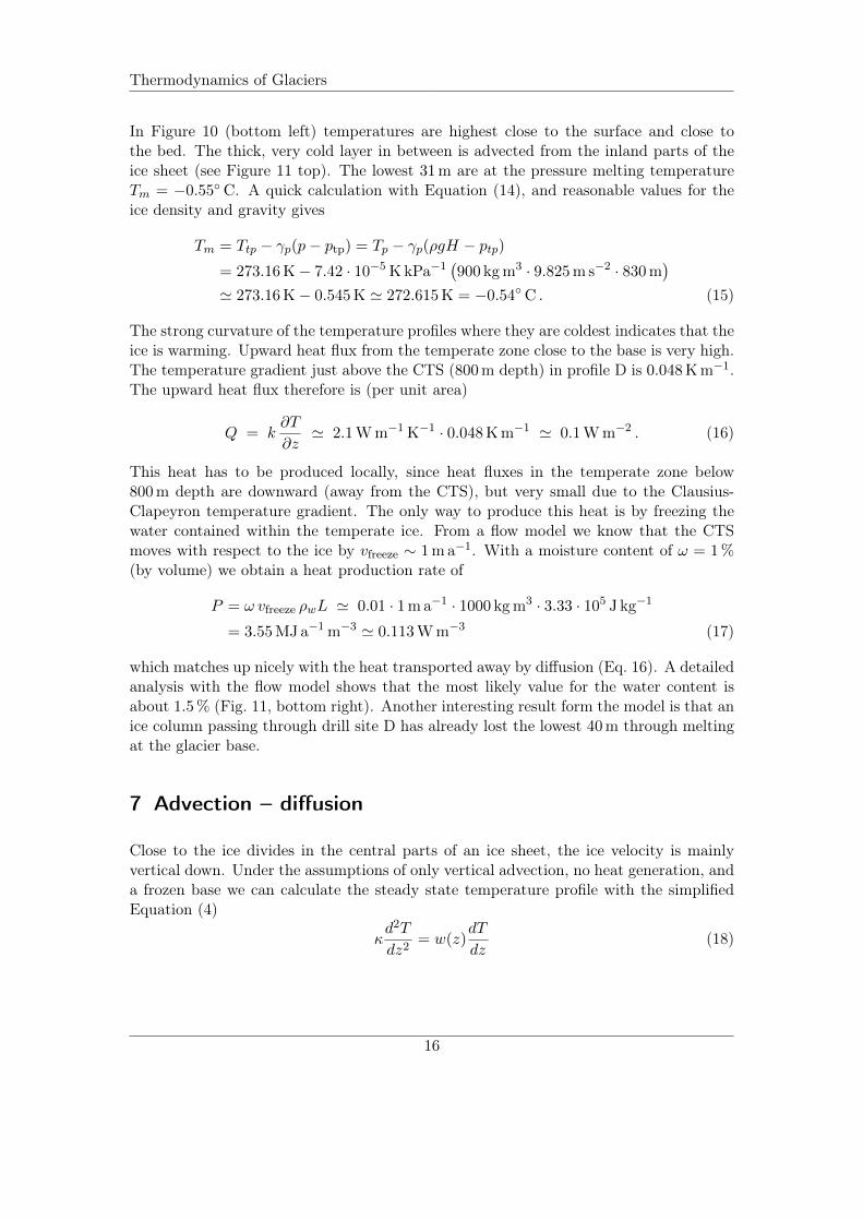
In Figure 10 (bottom left) temperatures are highest close to the surface and close tothe bed. The thick, very cold layer in between is advected from the inland parts of theice sheet (see Figure 11 top). The lowest 31 m are at the pressure melting temperatureTm = −0.55◦C. A quick calculation with Equation (14), and reasonable values for theice density and gravity gives

Tm = Ttp − γp(p− ptp) = Tp − γp(ρgH − ptp)= 273.16 K− 7.42 · 10−5 K kPa−1

(900 kg m3 · 9.825 m s−2 · 830 m

)' 273.16 K− 0.545 K ' 272.615 K = −0.54◦C . (15)

The strong curvature of the temperature profiles where they are coldest indicates that theice is warming. Upward heat flux from the temperate zone close to the base is very high.The temperature gradient just above the CTS (800 m depth) in profile D is 0.048 K m−1.The upward heat flux therefore is (per unit area)

Q = k∂T

∂z' 2.1 W m−1 K−1 · 0.048 K m−1 ' 0.1 W m−2 . (16)

This heat has to be produced locally, since heat fluxes in the temperate zone below800 m depth are downward (away from the CTS), but very small due to the Clausius-Clapeyron temperature gradient. The only way to produce this heat is by freezing thewater contained within the temperate ice. From a flow model we know that the CTSmoves with respect to the ice by vfreeze ∼ 1 m a−1. With a moisture content of ω = 1 %(by volume) we obtain a heat production rate of

P = ω vfreeze ρwL ' 0.01 · 1 m a−1 · 1000 kg m3 · 3.33 · 105 J kg−1

= 3.55 MJ a−1 m−3 ' 0.113 W m−3 (17)

which matches up nicely with the heat transported away by diffusion (Eq. 16). A detailedanalysis with the flow model shows that the most likely value for the water content isabout 1.5 % (Fig. 11, bottom right). Another interesting result form the model is that anice column passing through drill site D has already lost the lowest 40 m through meltingat the glacier base.

7 Advection – diffusion

Close to the ice divides in the central parts of an ice sheet, the ice velocity is mainlyvertical down. Under the assumptions of only vertical advection, no heat generation, anda frozen base we can calculate the steady state temperature profile with the simplifiedEquation (4)

κd2T

dz2= w(z)

dT

dz(18)

16


The boundary conditions are

surface: z = H : temperature Ts = const

bedrock: z = 0 : heat flux − k(dT

dz

)B

= G = const

For the first integration we substitute f = dTdz so that κf ′ = wf =⇒ f ′

f = 1κw with the

solutiondT (z)

dz=

(dT

dz

)B

exp

(1

κ

∫ z

0w(z) dz

). (19)

Now we make the assumption that the vertical velocity is w(z) = −bz/H, with thevertical velocity at the surface equal to the net mass balance rate ws = −b. With thedefinition l2 := 2κH/b we get

T (z)− T (0) =

(dT

dz

)B

∫ z

0exp

(−z

2

l2

)dz (20)

which has the solution

T (z)− Ts =

√π

2l

(dT

dz

)B

[erf(zl

)− erf

(H

l

)]. (21)

The so-called error function is tabulated and implemented in any mathematical software(usually as erf), and is defined as

erf(x) =2√π

∫ x

0exp(−x2) dx.

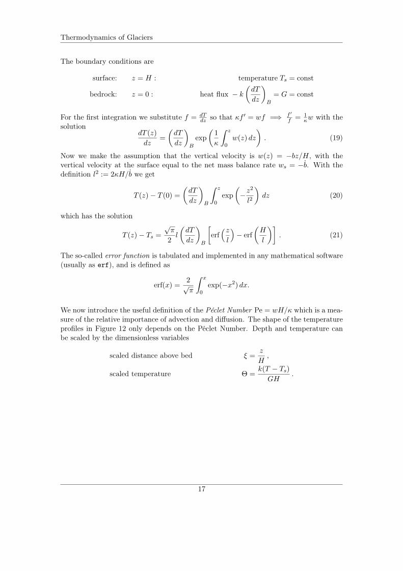
We now introduce the useful definition of the Péclet Number Pe = wH/κ which is a mea-sure of the relative importance of advection and diffusion. The shape of the temperatureprofiles in Figure 12 only depends on the Péclet Number. Depth and temperature canbe scaled by the dimensionless variables

scaled distance above bed ξ =z

H,

scaled temperature Θ =k(T − Ts)GH

.

17


0.0 0.2 0.4 0.6 0.8Scaled temperature Θ

0.0

0.2

0.4

0.6

0.8

1.0

Scal

edde

pth

ξ

0.00.5

13

510

2030

Figure 12: Dimensionless steady temperature profiles in terms of the dimensionless variables ξand Θ for various values of the Péclet number Pe (next to curves).

18


Literature

Bamber, J. L. (1988), Internal reflecting layers in Spitsbergen glaciers., Ann. Glaciol., 9,5–10.

Blatter, H. (1987), On the thermal regime of an arctic valley glacier, a study of the WhiteGlacier, Axel Heiberg Island, N.W.T., Canada, J. Glaciol., 33, 200–211.

Blatter, H., and G. Kappenberger (1988), Mass balance and thermal regime of Laika icecap, Coburg Island, N.W.T., Canada, J. Glaciol., 34, 102–110.

Breuer, B., M. A. Lange, and N. Blindow (2006), Sensitivity studies on model modifi-cations to assess the dynamics of a temperate ice cap, such as that on King GeorgeIsland, Antarctica, J. Glaciol., 52, 235–247.

Classen, D. F., and G. K. C. Clarke (1971), Basal hot spot on a surge type glacier,Nature, 229, 481–483.

Duval, P. (1977), The role of water content on the creep rate of polycrystalline ice, inIsotopes and impurities in snow and ice, pp. 29–33.

Eisen, O., M. P. Lüthi, P. Riesen, and M. Funk (2009), Deducing the thermal struc-ture in the tongue of Gornergletscher, Switzerland, from radar surveys and boreholemeasurements., Ann. Glaciol., 50 (51), 63–70.

Fountain, A. G., and J. S. Walder (1998), Water flow through temperate glaciers, Reviewsof Geophysics, 36, 299–328.

Fountain, A. G., R. W. Jacobel, R. Schlichting, and P. Jansson (2005), Fractures as themain pathways of water flow in temperate glaciers., Nature, 433, 618–621.

Funk, M., K. Echelmeyer, and A. Iken (1994), Mechanisms of fast flow in JakobshavnsIsbrae, Greenland; Part II: Modeling of englacial temperatures, J. Glaciol., 40, 569–585.

Greve, R., and H. Blatter (2009), Dynamics of Ice Sheets and Glaciers, Advances inGeophysical and Enviornmental Mechanics and Mathematics, Springer Verlag.

Gusmeroli, A., T. Murray, P. Jansson, R. Pettersson, A. Aschwanden, and A. D. Booth(2010), Vertical distribution of water within the polythermal Storglaciären, Sweden,J. Geophys. Res., in press.

Harrison, W. D. (1975), Temperature measurements in a temperate glacier, J. Glaciol.,14, 23–30.

Holmlund, P., and M. Eriksson (1989), The cold surface layer on Storglaciären., Ge-ographiska Annaler, 71A, 241–244.

19


Iken, A., K. Echelmeyer, M. Funk, and W. D. Harrison (1993), Mechanisms of fast flowin Jakobshavns Isbrae, Greenland, Part I: Measurements of temperature and waterlevel in deep boreholes, J. Glaciol., 39, 15–25.

Jania, J., D. Mochnacki, and B. Gadek (1996), The thermal structure of Hansbreen, atidewater glacier in southern Spitsbergen, Svalbard, Polar Research, 15, 53–66.

Lliboutry, L. A. (1976), Physical processes in temperate glaciers, J. Glaciol., 16, 151–158.

Lüthi, M. P., and M. Funk (2001), Modelling heat flow in a cold, high altitude glacier:interpretation of measurements from Colle Gnifetti, Swiss Alps, J. Glaciol., 47, 314–324.

Lüthi, M. P., M. Funk, A. Iken, M. Truffer, and S. Gogineni (2002), Mechanisms offast ow in Jakobshavns Isbræ, Greenland, Part III: measurements of ice deformation,temperature and cross-borehole conductivity in boreholes to the bedrock, J. Glaciol.,48 (162), 369–385.

Mader, H. M. (1992), Observations of the water-vein system in polycrystalline ice, J.Glaciol., 38 (130), 333–347.

Nye, J. F. (1989), The geometry of water veins and nodes in polycrystalline ice, J.Glaciol., 35 (119), 17–22.

Paterson, W. S. B. (1971), Temperature measurements in Athabasca Glacier, Alberta,Canada, J. Glaciol., 10, 339–349.

Paterson, W. S. B. (1994), The Physics of Glaciers, 480 pp., Pergamon, New York.

Pettersson, R., P. Jansson, and H. Blatter (2004), Spatial variability in water contentat the cold-temperate transition surface of the polythermal Storglaciären, Sweden., J.Geophys. Res., 109 (F2), 1–12, doi:10.1029/2003JF000110.

Raymond, C. F., and W. D. Harrison (1975), Some observations on the behaviour of theliquid and gas phases in temperate glacier ice, J. Glaciol., 14, 213–233.

Ritz, C. (1987), Time dependent boundary conditions for calculation of temperature fieldsin ice sheets, in The Physical Basis of Ice Sheet {M}odelling, vol. 170, pp. 207–216,Vancouver.

Ryser, C. (2009), The polythermal structure of Grenzgletscher, Valais, Switzerland, Mas-ter thesis, ETH Zurich.

20

Documents

Thermodynamics of Glaciers of Glaciers ... 1. ThermodynamicsofGlaciers ... Canadian-type glaciers are mostly cold 10. ThermodynamicsofGlaciers