67

S. Ishiwata and Y. Matsunaga, EditorsPhysics of Self-Organization Systems(World Scientific, New Jersey, 2008) pp. 67-87

THERMODYNAMIC TIME ASYMMETRY ANDNONEQUILIBRIUM STATISTICAL MECHANICS

Pierre GASPARD

Center for Nonlinear Phenomena and Complex Systems,Universite Libre de Bruxelles, Code Postal 231, Campus Plaine, B-1050 Brussels,

Belgium

A review of recent advances in nonequilibrium statistical mechanics is pre-

sented. These new results explain how the time reversal symmetry is broken inthe statistical description of nonequilibrium processes and the thermodynamic

entropy production finds its origin in the time asymmetry of nonequilibrium

fluctuations. These advances are based on new relationships expressing the timeasymmetry in terms of the temporal disorder and the probability distributions

of nonequilibrium fluctuations. These relationships apply to driven Brownian

motion and molecular motors.

Keywords: microreversibility, entropy production, relaxation, diffusion, out-of-

equilibrium nanosystems.

1. Introduction

Nonequilibrium statistical mechanics is undergoing tremendous advanceswith the discovery of universal relationships ruling molecular fluctuationsnear and far from equilibrium. These new relationships have been discov-ered thanks to dynamical systems theory where new concepts have beenintroduced to understand chaotic behavior. In this context, the issue of theinitial conditions of a dynamical system has been discussed about the phe-nomenon of sensitivity to initial conditions. The focus on this issue havedisclosed striking features on the role of initial conditions in the time asym-metry of nonequilibrium processes.

It is our purpose to give an overview of these recent results and their ap-plications to out-of-equilibrium nanosystems. Indeed, at the nanoscale, thefluctuations can no longer be neglected as it is the case at the macroscale.Accordingly, the processes taking place in nanosystems should be describedin terms of the probability distributions of molecular fluctuations. The fact

68

is that many nanosystems find their relevance because they function un-der nonequilibrium conditions, as for molecular motors or electronic con-ducting nanodevices. The new advances in nonequilibrium statistical me-chanics thus establish the bases for a statistical thermodynamics of out-of-equilibrium nanosystems. Remarkably, these recent developments pro-vide an unprecedented insight into our understanding of biological phenom-ena from the viewpoint of statistical thermodynamics. This insight extendsmuch beyond the already important results obtained with the macroscopicthermodynamics of irreversible processes [1], which did not deal with thefluctuations and their temporal properties. By carrying out the connec-tion between the macroscale and the molecular aspects at the nanoscale,nonequilibrium statistical mechanics is nowadays able to bridge the gaps be-tween molecular biology, bioenergetics, and the thermodynamic laws thanksto the advent of the new results about nonequilibrium fluctuations.

The review is organized as follows. The breaking of time reversal sym-metry in nonequilibrium statistical mechanics is discussed in Sec. 2 andillustrated in Sec. 3 with the relaxation modes of diffusion. We explain inSec. 4 how the thermodynamic arrow of time finds its origin in the timeasymmetry of temporal disorder in nonequilibrium fluctuations. In Sec. 5,we give an overview of the so-called fluctuation theorems. The case of molec-ular motors is presented in Sec. 6. Conclusions and perspectives are givenin Sec. 7.

2. The breaking of time reversal symmetry innonequilibrium statistical mechanics

The second law of thermodynamics is expressed in terms of the conceptof entropy. This quantity was interpreted by Boltzmann as a characteri-zation of the disorder in the probability distribution of the positions andvelocities of the particles composing the system. Later, Gibbs pointed outthat the microscopic definition of entropy requires coarse graining in oneway or another. There exist different versions of coarse graining. The firstwas introduced by Boltzmann who obtained his famous H-theorem by de-scribing dilute gases in terms of one-particle distributions. In this way, heneglected the statistical correlations between several particles, which maybe justified for dilute gases but allows the corresponding entropy to vary intime. Another version consists in tracing out the degrees of freedom of theenvironment of a subsystem, as done for a Brownian particle. In fine, thephase space can be partitioned into grains or cells to get the occupationprobabilities of these cells, as suggested by Gibbs in 1902. Since the work

69

of Sadi Carnot, coarse graining is inherently associated with the idea ofentropy because the efficiency of steam engines is a property of the steammicroscopic degrees of freedom manipulated by some macroscopic pistonon a very coarse-grained level. Only the coarse-grained entropy may evolvein time as the consequence of the dynamical property of mixing, also in-troduced by Gibbs. Indeed, the fine-grained entropy remains constant intime.

However, the breaking of the time reversal symmetry can be formulatedin nonequilibrium statistical mechanics at a more fundamental level with-out referring from the start to the thermodynamic entropy, but insteaddiscussing the symmetry of the probability distribution of the positions rand velocities v of the particles in classical mechanics:

p(Γ; t) = p(r,v; t) (1)

or the matrix density in quantum mechanics. These quantities obey timeevolution equations that is the Liouville equation for classical systems:

∂t p = {H, p}Poisson ≡ L p (2)

where {H, ·}Poisson denotes the Poisson bracket with the Hamiltonian func-tion H, or the Landau-von Neumann equation for quantum systems. Ac-tually, the time evolution of the probability distribution is induced by thedeterministic equations of motion which are Newton’s or Hamilton’s equa-tions of classical mechanics and Schrodinger’s equation of quantum mechan-ics. These equations are deterministic in the sense that their solutions areuniquely given in terms of their initial conditions according to Cauchy’stheorem. In classical systems, the initial condition is a point Γ = (r,v)taken in the phase space of the positions and velocities of the particleswhile the initial condition is a wavefunction taken in the Hilbert space of aquantum system.

Probability distributions are introduced because the initial state cannever be prepared with an infinite precision on uncountable continua suchas phase spaces or Hilbert spaces. On such continua, there is always adichotomy between the existence of a point-like initial condition and thenecessarily unprecise knowledge of this latter. As a result, the predictabil-ity of the trajectory becomes a concern in systems with sensitivity to ini-tial conditions – the so-called chaotic systems. Dynamical chaos guaranteesGibbs’ mixing property, which allows us to understand relaxation processesin many systems. It is also important to justify the use of a statistical de-scription in terms of probability distributions beyond the Lyapunov timecharacteristic of the sensitivity to initial conditions [2].

70

velocity v

position r

time reversal Θ

T = Θ(T')

T' = Θ(T )

0

(a)

velocity v

position r

time reversal Θ

0

(b)

•initial condition

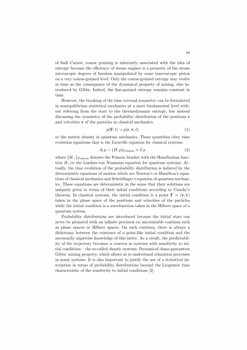
Fig. 1. (a) If Newton’s equation is time reversal symmetric, the time reversal Θ(T ) ofevery solution T is also a solution, as here shown in the phase space of the positions

and velocities of the system. (b) If the time reversal Θ(T ) is physically distinct from

the trajectory T , the selection of the trajectory T by the initial condition gives a unitprobability to T and zero to all the other solutions including the time reversal image

Θ(T ), therefore breaking the time reversal symmetry.

It turns out that the breaking of time reversal symmetry is another issueconcerning the initial conditions in chaotic as well as non-chaotic systems, asshown by the following discussion carried out in the framework of classicalmechanics. It is well known that Newton’s equation is symmetric undertime reversal:

Θ(r,v) = (r,−v) (3)

which leaves the positions r unchanged and reverses the velocities v =dr/dt, if the Hamiltonian is an even function of the velocities. The symmetry– called microreversibility – means that the time reversal of a solution ofNewton’s equation is also a solution of this equation (see Fig. 1a). Eachinitial condition selects a precise solution of Newton’s equations, whichdepicts a trajectory T = {Γ(t)|t ∈ R} in the phase space Γ = (r,v). Wemay say that a trajectory T is physically distinct from another trajectory

71

velocity v

position r

0

(a)

velocity v

position r

time reversal Θ

0

(b)

time reversal Θ

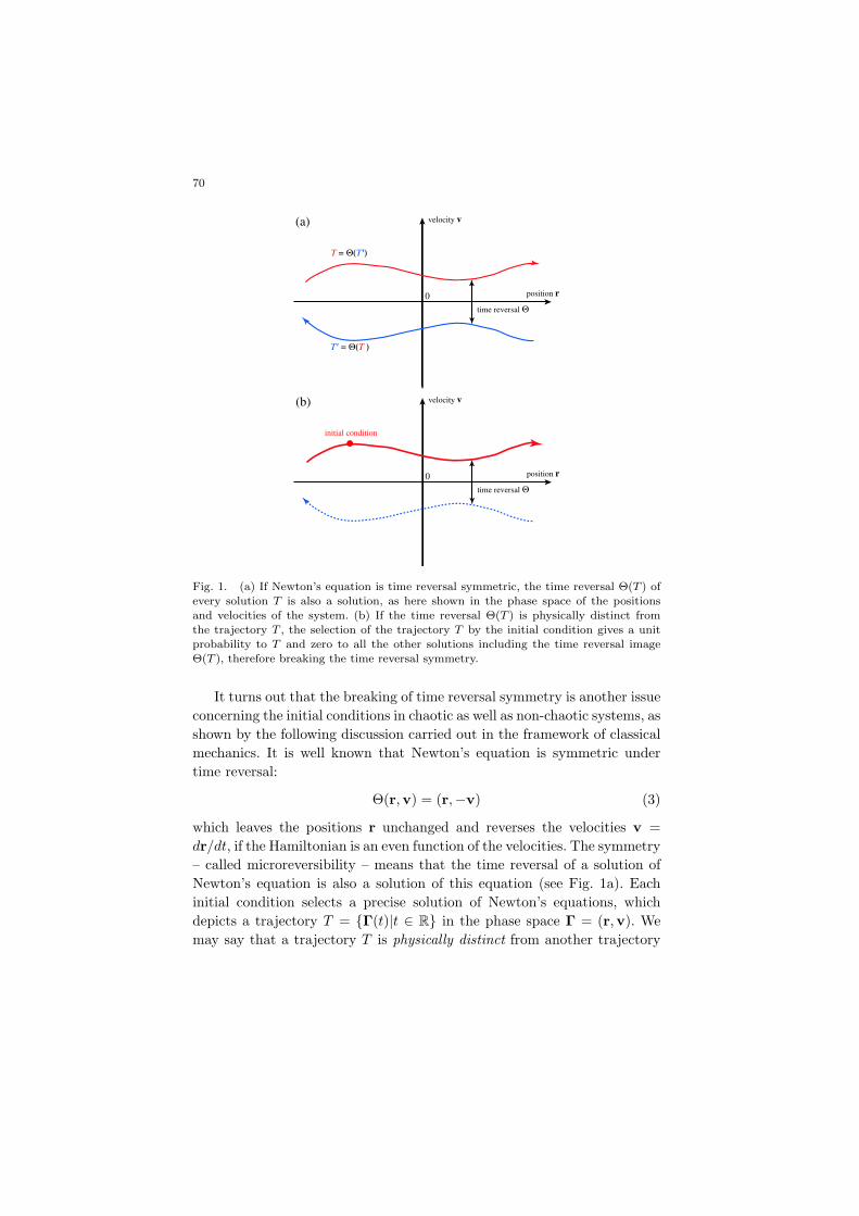
Fig. 2. (a) Phase portrait of the harmonic oscillator (4). All its trajectories are ellipseswhich are self-reversed. Consequently, the selection of an initial condition does not break

the time reversal symmetry in this system. (b) Phase portrait of the free particle (5).

Here, the trajectories are physically distinct from their image under time reversal, exceptif the velocity vanishes. Consequently, the selection of an initial condition (with a non-

vanishing velocity) breaks the time reversal symmetry in this system.

if they do not coincide in the phase space of the system.If the trajectory T followed by the system during its time evolution

is physically distinct from its time reversal, Θ(T ) 6= T , it turns out thatthe time reversal symmetry is broken in the system. This is the same asfor other symmetry breaking phenomena in condensed matter physics. Forinstance, the double-well potential V (x) = (x2/2) − (x4/4) is symmetricunder parity x → −x. This symmetry is broken if the system is found inone of the wells, either x = +1 or x = −1. This illustrates the generalresult that the solution of an equation may have a lower symmetry thanthe equation itself. This phenomenon of symmetry breaking applies to timereversal as well. Although Newton’s equation is time reversal symmetric, itssolutions do not necessarily have the symmetry. Therefore, the selection ofa trajectory by the initial condition can break the time reversal symmetry.

72

velocity v

position r

time reversal Θ

0

(a)

velocity v

position r0

(b)

rese

rvoir

1reserv

oir 2

time reversal Θ

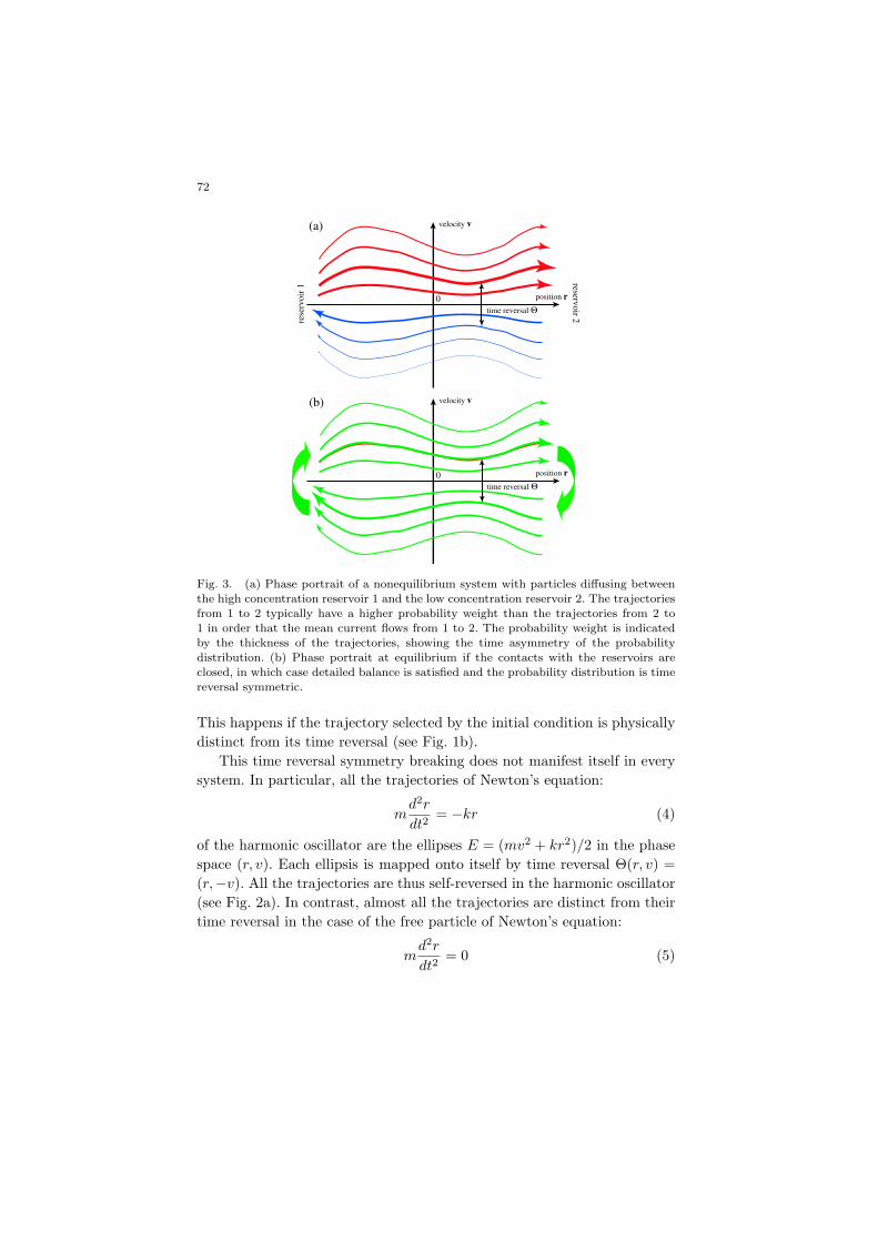
Fig. 3. (a) Phase portrait of a nonequilibrium system with particles diffusing between

the high concentration reservoir 1 and the low concentration reservoir 2. The trajectories

from 1 to 2 typically have a higher probability weight than the trajectories from 2 to1 in order that the mean current flows from 1 to 2. The probability weight is indicated

by the thickness of the trajectories, showing the time asymmetry of the probability

distribution. (b) Phase portrait at equilibrium if the contacts with the reservoirs areclosed, in which case detailed balance is satisfied and the probability distribution is time

reversal symmetric.

This happens if the trajectory selected by the initial condition is physicallydistinct from its time reversal (see Fig. 1b).

This time reversal symmetry breaking does not manifest itself in everysystem. In particular, all the trajectories of Newton’s equation:

md2r

dt2= −kr (4)

of the harmonic oscillator are the ellipses E = (mv2 + kr2)/2 in the phasespace (r, v). Each ellipsis is mapped onto itself by time reversal Θ(r, v) =(r,−v). All the trajectories are thus self-reversed in the harmonic oscillator(see Fig. 2a). In contrast, almost all the trajectories are distinct from theirtime reversal in the case of the free particle of Newton’s equation:

md2r

dt2= 0 (5)

73

Indeed, the trajectories are the straight lines r(t) = r(0)+v(0)t, v(t) = v(0),which are distinct from their reversal if the velocity is non vanishing,v(0) 6= 0 (see Fig. 2b). Therefore, the selection of an initial condition mayalready break the time reversal symmetry in this simple system. A fortiori,this breaking can also happen in a chaotic system with a spectrum of posi-tive Lyapunov exponents indicating many stable and unstable directions inphase space. These directions are mapped onto each other but physicallydistinct so that the time reversal symmetry will be broken if one specificdirection is selected by the initial condition [3,4].

In statistical mechanics, each initial condition – and thus each phase-space trajectory – is weighted with a probability giving its statistical fre-quency of occurrence in a sequence of repeated experiments. This is inparticular the case for a nonequilibrium system with particles diffusing be-tween two reservoirs at different concentrations. After some transients, thesystem reaches a nonequilibrium steady state which can be described byan invariant probability distribution. Averaging over this distribution givesa mean current of diffusing particles from high to low concentrations. Inthis case, the phase-space trajectories issued from the high concentrationreservoir typically have a higher probability weight than the trajectoriesfrom the low concentration reservoir (see Fig. 3a). Since the set of theselatter trajectories contain the time reversal of the former ones, we concludethat the time reversal symmetry is broken by the nonequilibrium invariantprobability distribution:

pneq(ΘΓ) 6= pneq(Γ) (6)

Of course, if the contacts with the reservoirs are closed, the invariant prob-ability becomes the equilibrium one after relaxation, in which case detailedbalance is satisfied and the time reversal symmetry is restored:

peq(ΘΓ) = peq(Γ) (7)

(see Fig. 3b). Since the nonequilibrium invariant probability distributionsare stationary solutions of Liouville’s equation (2), we here have a similarsymmetry breaking phenomenon as for Newton’s equation. The nonequi-librium stationary density (6) is a solution of Liouville’s equation with alower symmetry than the equation itself. In this way, irreversible behaviorcan be described by weighting differently the trajectories T and their timereversal images Θ(T ) with a probability measure.

74

3. The relaxation modes of diffusion

In this section, we show in specific systems that the breaking of time re-versal symmetry is indeed the fact of systems in nonequilibrium states. Weconsider Hamiltonian systems with chaotic diffusion such as the multibakermap [5–7], the hard-disk Lorentz gas, and the Yukawa-potential Lorentzgas [8]. The Newtonian dynamics of these systems is Hamiltonian and timereversal symmetric. These systems sustain the transport property of diffu-sion because of their spatial extension. Moreover, the dynamics is periodicin space as for the motion of electrons or impurities in a crystal.

If the initial conditions are taken out of equilibrium, the probabilitydistribution undergoes a transient relaxation toward a uniform state cor-responding to the thermodynamic equilibrium. This relaxation can be de-composed into modes which are special solutions of Liouville’s equation(2):

p(r,v; t) = C exp(skt) Ψk(r,v) (8)

These solutions are spatially periodic Ψk(r,v) ∼ exp(ik · r) with a wave-length λ = 2π/k typically much longer than the periodicity of the crystal.The solutions (8) are exponentially damped in time at the rate

−sk = Dk2 + O(k4) (9)

vanishing quadratically with the wavenumber k, which defines the diffusioncoefficient given by the Green-Kubo formula:

D =∫ ∞

0

〈vx(0)vx(t)〉eq dt (10)

It turns out that the relaxation modes (8) can be constructed in phasespace as generalized eigenstates of the Liouvillian operator of Eq. (2):

LΨk = skΨk (11)

with the associated eigenvalue sk given by a so-called Pollicott-Ruelle res-onance [2]. The generalized eigenstates Ψk do not exist as functions but asdistributions of Schwartz type, which are defined on some functional spaceof test functions. The remarkable feature of the construction is that it canbe carried out without a specific coarse graining since the distribution Ψk

is defined on a whole functional space of possible test functions. The useof such test functions may be considered as coarse graining but the gener-alized eigenstate does not depend on the choice of a specific test functiontaken in the functional space.

75

. . . . . .

ll−1 l+1. . .. . .

Re F

Im F

k

Re F

Im F

k

Re F

Im F

k

(a)

(b)

(c)

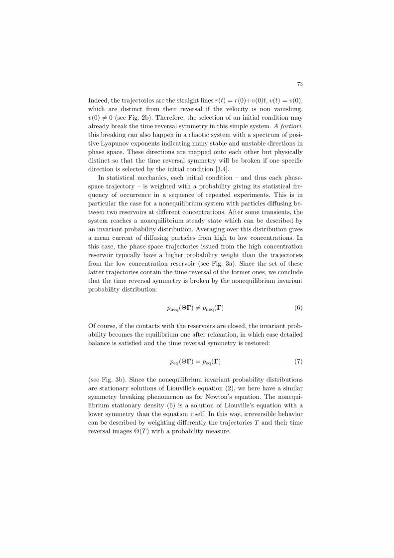
Fig. 4. The relaxation modes of diffusion in (a) the multibaker map [5–7], (b) the hard-disk Lorentz gas, and (c) the Yukawa-potential Lorentz gas [8]. The left-hand column

shows the mechanism of diffusion of particles in these systems. In the right-hand column,the cumulative function (12) is depicted in the complex plane (Re F, Im F ) versus the

wavenumber k, for each system. If the wavenumber vanishes k = 0, the cumulativefunction reduces to the straight line Im F = 0 between the points Re F = 0 and Re F = 1,which represents the microcanonical equilibrium state.

76

The densities Ψk(r,v) are singular along the stable manifolds Ws ofphase space, but nevertheless smooth along the unstable manifolds Wu.Since the stable and unstable manifolds are mapped onto each other bytime reversal Wu = Θ(Ws), but are physically distinct Wu 6= Ws, the densi-ties Ψk(r,v) are solutions of Liouville’s equation which break the time re-versal symmetry, as expected for solutions corresponding to unidirectionalexponential decay. The time asymmetry of the relaxation modes can be dis-played by explicitly constructing the eigenstates thanks to their cumulativefunction

Fk(θ) =∫ θ

0

Ψk(rθ′ ,vθ′) dθ′ = limt→∞

∫ θ

0exp [ik · (rt − r0)θ′ ] dθ′∫ 2π

0exp [ik · (rt − r0)θ′ ] dθ′

(12)

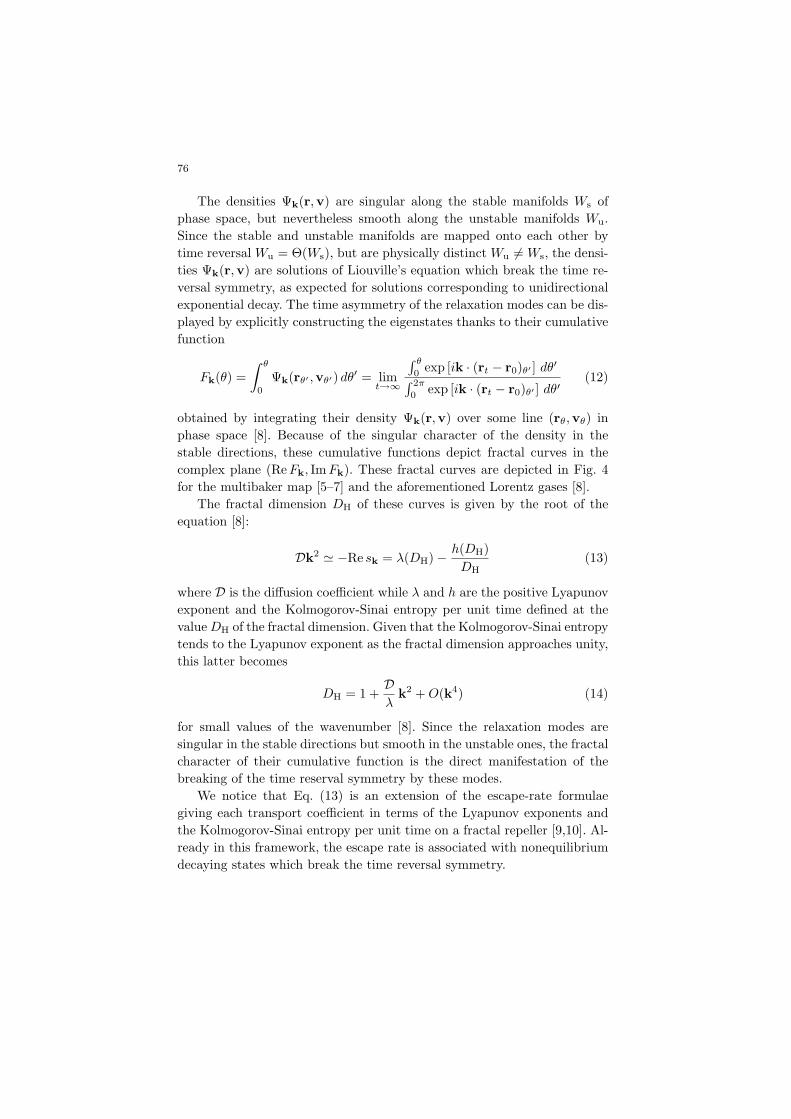
obtained by integrating their density Ψk(r,v) over some line (rθ,vθ) inphase space [8]. Because of the singular character of the density in thestable directions, these cumulative functions depict fractal curves in thecomplex plane (Re Fk, Im Fk). These fractal curves are depicted in Fig. 4for the multibaker map [5–7] and the aforementioned Lorentz gases [8].

The fractal dimension DH of these curves is given by the root of theequation [8]:

Dk2 ' −Re sk = λ(DH)− h(DH)DH

(13)

where D is the diffusion coefficient while λ and h are the positive Lyapunovexponent and the Kolmogorov-Sinai entropy per unit time defined at thevalue DH of the fractal dimension. Given that the Kolmogorov-Sinai entropytends to the Lyapunov exponent as the fractal dimension approaches unity,this latter becomes

DH = 1 +Dλ

k2 + O(k4) (14)

for small values of the wavenumber [8]. Since the relaxation modes aresingular in the stable directions but smooth in the unstable ones, the fractalcharacter of their cumulative function is the direct manifestation of thebreaking of the time reserval symmetry by these modes.

We notice that Eq. (13) is an extension of the escape-rate formulaegiving each transport coefficient in terms of the Lyapunov exponents andthe Kolmogorov-Sinai entropy per unit time on a fractal repeller [9,10]. Al-ready in this framework, the escape rate is associated with nonequilibriumdecaying states which break the time reversal symmetry.

77

The density of the nonequilibrium steady state of gradient g can beobtained from the densities (8) of the relaxation modes according to

Ψg(Γ) = −ig · ∂

∂kΨk(Γ)

∣∣∣k=0

= g ·[r(Γ) +

∫ −∞

0

v(ΦtΓ) dt

](15)

where Φt denotes the Hamiltonian flow [6]. Because of Eq. (15), thenonequilibrium steady states have similar singularities as the relaxationmodes. Their distribution is smooth along the unstable manifolds but sin-gular in the stable directions. Their cumulative function is the nondiffer-entiable Takagi function in the multibaker map and its generalizations inthe Lorentz gases [6]. This singular character is thus the manifestation ofthe breaking of the time reversal symmetry by the invariant probabilitydistribution of nonequilibrium steady states.

4. Experimental evidence of the time asymmetry ofnonequilibrium fluctuations

The breaking of the time reversal symmetry by the invariant probabilitydistribution describing the nonequilibrium steady states has direct experi-mental consequences, which have been evidenced in recent experiments inthe group of Professor Sergio Ciliberto at the ENS of Lyon (France) on thedriven Brownian motion of a micrometric particle trapped by an opticaltweezer in a moving fluid and the Nyquist thermal noise of a RC electriccircuit driven out of equilibrium by a current [11,12].

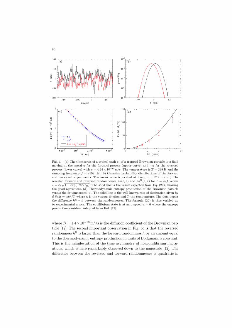
In driven Brownian motion, the position of the particle can be monitoredwith nanometric resolution thanks to an interferometer. Long time seriesof the position of the Brownian particle have been recorded in the frameof the optical trap for a driving by the surrounding fluid with the speedsu and −u. Examples of such paths are depicted in Fig. 5a. Figure 5b givesthe corresponding stationary probability distributions of the position z,showing the effect of the drag due to the moving fluid. The observationsare well described by an overdamped Langevin equation including the forceexerted by the potential of the laser trap, the drag force of the moving fluid,the viscous firction force, and the Langevin force of the thermal fluctuations[11,12]. The long time series allow us to measure the probabilities of pathsωωω = ω0ω1ω2 . . . ωn−1 of varying resolution ε on the position and sampledevery time interval τ . We can compare the probability of a path in theprocess of speed u with the probability of the time-reversed path ωωωR =ωn−1 . . . ω2ω1ω0 in the process of opposite speed −u. As for the trajectories,a time-reversed path is typically distinct from the corresponding path, ωωωR 6=

78

ωωω. The coincidence only happens for the rare self-reversed paths. Accordingto detailed balance, we expect that the probabilities of the paths and theirtime reversal are equal if u = 0:

equilibrium: P0(ω0ω1 . . . ωn−1) = P0(ωn−1 . . . ω1ω0) (16)

However, this equality is not expected if u 6= 0:

out of equilibrium: Pu(ω0ω1 . . . ωn−1) 6= P−u(ωn−1 . . . ω1ω0) (17)

This difference also affects the decay of these path probabilities. Their meandecay rates characterize the temporal disorder or dynamical randomnessand are called the (ε, τ)-entropy per unit time [13]:

h = limn→∞

− 1nτ

∑ω0ω1...ωn−1

Pu(ω0ω1 . . . ωn−1) lnPu(ω0ω1 . . . ωn−1) (18)

and time-reversed (ε, τ)-entropy per unit time [14]:

hR = limn→∞

− 1nτ

∑ω0ω1...ωn−1

Pu(ω0ω1 . . . ωn−1) lnP−u(ωn−1 . . . ω1ω0) (19)

The supremum of the dynamical entropy (18) over all the possible coarsegrainings defines the famous Kolmogorov-Sinai entropy per unit time, whichequals the sum of positive Lyapunov exponents in closed dynamical systemsaccording to Pesin’s theorem [2]. Instead, the time-reversed entropy per unittime (19) has been recently introduced motivated by the difference (17) ex-pected in nonequilibrium processes [14]. Contrary to the thermodynamicentropy which measures the disorder of the probability distribution in thephase space at a given time, the entropies per unit time characterize thedisorder displayed by the process along the time axis, as in the successivepictures of a movie. We thus speak of temporal disorder or dynamical ran-domness for the property characterized by the quantities (18) and (19). Toavoid a possible confusion with the standard thermodynamic entropy, weshall respectively call them the forward and reversed randomnesses in thefollowing.

The most remarkable result is that the difference between these ran-domnesses gives the thermodynamic entropy production according to

1kB

diS

dt= lim

ε,τ→0

[hR(ε, τ)− h(ε, τ)

]≥ 0 (20)

where kB is Boltzmann’s constant [14]. This difference is the Kullback-Leibler distance between the path probabilities Pu(ωωω) and P−u(ωωωR), also

79

known under the name of relative entropy, and is therefore always non-negative in agreement with the second law of thermodynamics. The formula(20) is remarkable because it connects the arrow of time of macroscopic ther-modynamics to another arrow of time observed at the mesoscopic scales inthe temporal disorder of the nonequilibrium fluctuations. The time asym-metry of this temporal disorder manifests itself in the difference hR − h.The formula (20) thus shows that the thermodynamic arrow of time findsits origin in the time asymmetry of temporal disorder in the nonequilibriumfluctuations.

The formula (20) is also remarkable because it provides a rational foun-dation to the intuitive idea that dynamical order arises in a system drivenout of equilibrium, as expressed by the

Theorem of nonequilibrium temporal ordering [15]: In nonequi-librium steady states, the typical paths are more ordered in time than theircorresponding time reversals in the sense that their temporal disorder char-acterized by h is smaller than the temporal disorder of the correspondingtime-reversed paths characterized by hR.

This theorem expresses the fact that the molecular motions are com-pletely erratic at equilibrium, albeit they acquire a privileged direction andare thus more ordered out of equilibrium. This happens because of the timeasymmetric selection of initial conditions under nonequilibrium conditions,resulting into an invariant probability distribution which breaks the timereversal symmetry by favoring some trajectories with respect to their timereversal images. The temporal ordering is possible at the expense of the in-crease of the phase-space disorder and is thus compatible with Boltzmann’sinterpretation of the second law.

The time asymmetry of temporal disorder has been observed for drivenBrownian motion in the aforementioned experiments [11,12]. Figure 5c de-picts the forward and reversed randomnesses versus the rescaled resolu-tion δ = ε/

√1− exp(−2τ/τR) where τR ' 3 ms is the relaxation time of

the Brownian particle in the laser trap. First of all, we observe that thesequantities increase as the resolution goes down to the scale of nanometers,reached thanks to the interferometric techniques [11,12]. This means thatthe stochastic process of Brownian motion generates more and more tem-poral disorder as the process is observed on smaller and smaller scales ε.For small values of the spatial resolution ε, we find that

h(ε, τ) =1τ

ln

√πeDτR

2ε2

(1− e−2τ/τR

)+ O(ε2) (21)

80

0.9 0.95 1 1.05

time (s)

−100

−50

0

50

100

z

(n

m)

(a)

−100 0 100

z (nm)

10−6

10−5

10−4

10−3

10−2

pro

bab

ilit

y

(b)

0

1

2

5 10-9 10-8 2 10-8 5 10-8

τ h

τ hR

τ (h + kB

−1 diS/dt)

τ h

(ε,τ

)

&

τ h

R(ε

,τ)

δ

(m)

(c)

0 1 2 3 4 5

|u| (µm/s)

0

50

100

150

iS/d

t (k

BT

/s)

T d

(d)

Fig. 5. (a) The time series of a typical path zt of a trapped Brownian particle in a fluid

moving at the speed u for the forward process (upper curve) and −u for the reversedprocess (lower curve) with u = 4.24× 10−6 m/s. The temperature is T = 298 K and the

sampling frequency f = 8192 Hz. (b) Gaussian probability distributions of the forward

and backward experiments. The mean value is located at ±uτR = ±12.9 nm. (c) Therescaled forward and reversed randomnesses τh(ε, τ) and τhR(ε, τ) for τ = 4/f versus

δ = ε/p

1− exp(−2τ/τR). The solid line is the result expected from Eq. (20), showing

the good agreement. (d) Thermodynamic entropy production of the Brownian particleversus the driving speed |u|. The solid line is the well-known rate of dissipation given by

diS/dt = αu2/T where α is the viscous friction and T the temperature. The dots depict

the difference hR − h between the randomnesses. The formula (20) is thus verified upto experimental errors. The equilibrium state is at zero speed u = 0 where the entropy

production vanishes. Adapted from Ref. [12].

where D = 1.4×10−13 m2/s is the diffusion coefficient of the Brownian par-ticle [12]. The second important observation in Fig. 5c is that the reversedrandomness hR is larger than the forward randomness h by an amount equalto the thermodynamic entropy production in units of Boltzmann’s constant.This is the manifestation of the time asymmetry of nonequilibrium fluctu-ations, which is here remarkably observed down to the nanoscale [12]. Thedifference between the reversed and forward randomnesses is quadratic in

81

the fluid speed u as expected from viscous dissipation (see Fig. 5d).Similar results have been obtained for an RC electric circuit, showing

the time asymmetry down to fluctuations of about a few thousands elec-tronic charges [12]. The link between the formula (20) and the escape-ratetheory has been discussed elsewhere [4]. The connection can also be estab-lished with nonequilibrium work relations [16,17].

5. The fluctuation theorem

Another newly discovered relationship is the fluctuation theorem which con-cerns the probability distribution of fluctuating quantities such as the cur-rents crossing a nonequilibrium system, the corresponding dissipated heat,or the work performed on the system. Several versions of the fluctuationtheorem have been derived for either dynamical systems or stochastic pro-cesses [18–23]. The fluctuation theorem is based on the microreversibilityimplying a symmetry relation between the probabilities of opposite fluctu-ations.

Recently, we have carried out a derivation of the fluctuation theorem forstochastic processes in the framework of the graph theory by Hill, Schnaken-berg, and others [24–26]. This approach allows us to identify the thermo-dynamic forces – i.e., the De Donder affinities [27,28] – driving the systemout of equilibrium [29–31]. In chemical kinetics, the affinities are given interms of the free enthalpy changes of the reactions:

Aγ =∆Gγ

kBT=

Gγ −Gγ,eq

kBT(22)

where T is the temperature [27,28]. In electric devices, the affinities aregiven by the difference of electronic chemical potentials between the elec-tromotive sources of the circuit. If the affinities vanish, the system returnsto equilibrium. Therefore, these affinities drive nonequilibrium currents,which take fluctuating instantaneous values jγ(t). The average of such acurrent over a finite time interval t is thus the random variable:

Jγ =1t

∫ t

0

jγ(t′) dt′ (23)

In chemical reactions, these currents are the rates of the reactive events, i.e.,the rates of the transformations of reactants into products. In chemome-chanical systems such as the F1-ATPase rotary molecular motor, a currentmay represent the number of revolutions per unit time while another isthe rate of consumption or synthesis of ATP. Accordingly, the system may

82

sustain several currents J = (J1, J2, ..., Jγ , ..., Jc) driven by as many cor-responding affinities A = (A1, A2, ..., Aγ , ..., Ac). For the molecular motor,these affinities are respectively the external torque acting on its shaft andthe affinity of ATP hydrolysis (see below).

The fluctuation theorem for the currents asserts that the ratio of theprobabilities of opposite fluctuations goes exponentially with the time in-terval and the magnitude of the affinities and fluctuations:

P (J)P (−J)

' exp (A · J t) for t →∞ (24)

The statistical average of the argument in the exponential is nothing elseas the thermodynamic entropy production:

1kB

diS

dt= A · 〈J〉 ≥ 0 (25)

The fluctuation theorem for the currents allow us to obtain the general-izations of Onsager’s reciprocity relations to the nonlinear response coeffi-cients [29,31].

If we introduce the decay rate of the probability as P (J) ∼exp [−H(J) t], the fluctuation theorem can be expressed in the form:

A · J = H(−J)−H(J) (26)

which shows the similarity with the other new relationships that are theequations (13) and (20), as well as the escape-rate formulae [9,10]. If Eq.(26) is evaluated for the mean currents, the thermodynamic entropy pro-duction turns out to be given by H(−〈J〉) since H(〈J〉) = 0. Comparingwith Eq. (20), we infer that the reversed randomness is larger – and typi-cally much larger – than the decay rate of the opposite current probability:hR(ε, τ) ≥ H(−〈J〉). This shows that the probability distribution of the cur-rents characterizes the system in a coarser way than the (ε, τ)-entropies perunit time, which can even probe the fluctuations down to the nanoscale [12].In this sense, the fluctuation theorem is closer to the macroscale than therelationship (20) described in the previous section.

6. Molecular motors

The new advances reported in the previous sections apply to out-of-equilibrium nanosystems such as the molecular motors, characterizing theway they function in the presence of fluctuations. One of the best knownmolecular motors is the F1-ATPase studied by Professor Kinosita andcoworkers [32,33]. The F1-ATPase protein complex is a barrel composed

83

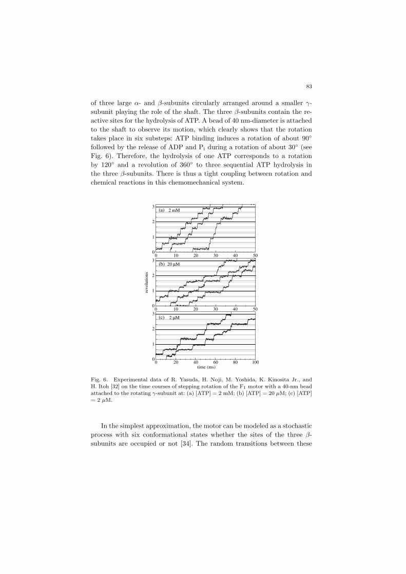
of three large α- and β-subunits circularly arranged around a smaller γ-subunit playing the role of the shaft. The three β-subunits contain the re-active sites for the hydrolysis of ATP. A bead of 40 nm-diameter is attachedto the shaft to observe its motion, which clearly shows that the rotationtakes place in six substeps: ATP binding induces a rotation of about 90◦

followed by the release of ADP and Pi during a rotation of about 30◦ (seeFig. 6). Therefore, the hydrolysis of one ATP corresponds to a rotationby 120◦ and a revolution of 360◦ to three sequential ATP hydrolysis inthe three β-subunits. There is thus a tight coupling between rotation andchemical reactions in this chemomechanical system.

1

2

3

revolu

tions

time (ms)

(a)

2 µM

0

1

2

320 µM

2 mM

0

1

2

3

00 10 20 30 40 50

0 10 20 30 40 50

0 20 40 60 80 100

(b)

(c)

Fig. 6. Experimental data of R. Yasuda, H. Noji, M. Yoshida, K. Kinosita Jr., and

H. Itoh [32] on the time courses of stepping rotation of the F1 motor with a 40-nm bead

attached to the rotating γ-subunit at: (a) [ATP] = 2 mM; (b) [ATP] = 20 µM; (c) [ATP]= 2 µM.

In the simplest approximation, the motor can be modeled as a stochasticprocess with six conformational states whether the sites of the three β-subunits are occupied or not [34]. The random transitions between these

84

0

0.05

0.1

0.15

0.2

0.25

-15 -10 -5 0 5 10 15

pro

bab

ilit

y

s

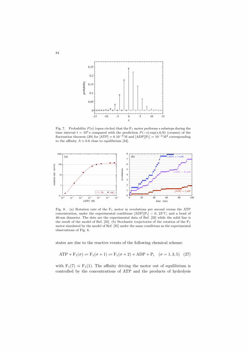
Fig. 7. Probability P (s) (open circles) that the F1 motor performs s substeps during the

time interval t = 104 s compared with the prediction P (−s) exp(sA/6) (crosses) of the

fluctuation theorem (29) for [ATP] = 6 10−8 M and [ADP][Pi] = 10−2 M2 correspondingto the affinity A ' 0.6 close to equilibrium [34].

0

1

2

3

4

5

6

7

8

0 20 40 60 80 100

rev

olu

tio

ns

time (ms)

[ATP] = 2 mM

[ATP] = 20 µM

[ATP] = 2 µM

0.1

1

10

100

1000

10-8 10-7 10-6 10-5 10-4 10-3 10-2

th. exp.

rota

tio

n r

ate

(r

ev/s

)

[ATP] (M)

(a) (b)

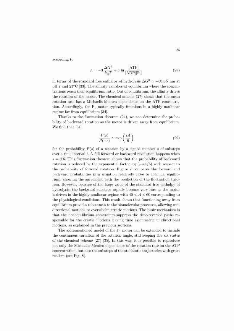
Fig. 8. (a) Rotation rate of the F1 motor in revolutions per second versus the ATPconcentration, under the experimental conditions [ADP][Pi] = 0, 23◦C, and a bead of40-nm diameter. The dots are the experimental data of Ref. [32] while the solid line is

the result of the model of Ref. [35]. (b) Stochastic trajectories of the rotation of the F1

motor simulated by the model of Ref. [35] under the same conditions as the experimentalobservations of Fig. 6.

states are due to the reactive events of the following chemical scheme:

ATP + F1(σ) F1(σ + 1) F1(σ + 2) + ADP + Pi (σ = 1, 3, 5) (27)

with F1(7) ≡ F1(1). The affinity driving the motor out of equilibrium iscontrolled by the concentrations of ATP and the products of hydrolysis

85

according to

A = −3∆G0

kBT+ 3 ln

[ATP][ADP][Pi]

(28)

in terms of the standard free enthalpy of hydrolysis ∆G0 ' −50 pN nm atpH 7 and 23◦C [33]. The affinity vanishes at equilibrium where the concen-trations reach their equilibrium ratio. Out of equilibrium, the affinity drivesthe rotation of the motor. The chemical scheme (27) shows that the meanrotation rate has a Michaelis-Menten dependence on the ATP concentra-tion. Accordingly, the F1 motor typically functions in a highly nonlinearregime far from equilibrium [34].

Thanks to the fluctuation theorem (24), we can determine the proba-bility of backward rotation as the motor is driven away from equilibrium.We find that [34]

P (s)P (−s)

' exp(

sA

6

)(29)

for the probability P (s) of a rotation by a signed number s of substepsover a time interval t. A full forward or backward revolution happens whens = ±6. This fluctuation theorem shows that the probability of backwardrotation is reduced by the exponential factor exp(−sA/6) with respect tothe probability of forward rotation. Figure 7 compares the forward andbackward probabilities in a situation relatively close to chemical equilib-rium, showing the agreement with the prediction of the fluctuation theo-rem. However, because of the large value of the standard free enthalpy ofhydrolysis, the backward substeps rapidly become very rare as the motoris driven in the highly nonlinear regime with 40 < A < 60 corresponding tothe physiological conditions. This result shows that functioning away fromequilibrium provides robustness to the biomolecular processes, allowing uni-directional motions to overwhelm erratic motions. The basic mechanism isthat the nonequilibrium constraints suppress the time-reversed paths re-sponsible for the erratic motions leaving time asymmetric unidirectionalmotions, as explained in the previous sections.

The aforementioned model of the F1 motor can be extended to includethe continuous variation of the rotation angle, still keeping the six statesof the chemical scheme (27) [35]. In this way, it is possible to reproducenot only the Michaelis-Menten dependence of the rotation rate on the ATPconcentration, but also the substeps of the stochastic trajectories with greatrealism (see Fig. 8).

86

7. Conclusions and perspectives

Recent progress in nonequilibrium statistical mechanics has achieved theintegration of thermodynamics with stochastic aspects in systems drivenout of equilibrium. In this regard, the new results provide the basis for anonequilibrium statistical thermodynamics of nanosystems bridging the gapbetween the emergent macroscopic phenomena and the molecular motionsat the nanoscale. The integration of thermodynamic and stochastic aspectshas been made possible thanks to the discovery of new relationships whichall share the same mathematical scheme in which an irreversible thermo-dynamic property is given by the difference between two quantities char-acterizing the randomness of molecular motions. This scheme appears inthe escape-rate formulae [9,10], Eqs. (13) and (20), as well as the form (26)of the fluctuation theorem. In this way, the thermodynamic entropy pro-duction can nowadays be understood as a time asymmetry in the temporaldisorder of nonequilibrium fluctuations.

These relationships concern the unidirectional motions of nonequilib-rium systems such as the driven Brownian motion and the F1-ATPasemolecular motor. Although their motions are erratic at equilibrium whereopposite random steps have equal probabilities, they become unidirectionalout of equilibrium by the time asymmetric suppression of backward steps,as explained thanks to the new relationships. These results open importantperspectives in our understanding of biological phenomena on the basis ofthermodynamics. Indeed, one of the main features of life is metabolism,which is the evidence of the many nonequilibrium processes taking placein cells. The recent results explain that this nonequilibrium regime is re-sponsible for temporal ordering in the behavior of biosystems. In this way,modern statistical thermodynamics can give an answer to the question ofthe origins of order and information in biological systems.

Acknowledgments

This research is financially supported by the F.R.S.-FNRS Belgium andthe “Communaute francaise de Belgique” (contract “Actions de RechercheConcertees” No. 04/09-312).

References

1. I. Prigogine, Introduction to Thermodynamics of Irreversible Processes (Wiley,New York, 1967).

2. P. Gaspard, Chaos, Scattering and Statistical Mechanics (Cambridge Univer-sity Press, Cambridge UK, 1998).

87

3. P. Gaspard, Physica A 369, 201 (2006).4. P. Gaspard, Adv. Chem. Phys. 135, 83 (2007).5. P. Gaspard, J. Stat. Phys. 68, 673 (1992).6. S. Tasaki and P. Gaspard, J. Stat. Phys. 81, 935 (1995).7. S. Tasaki and P. Gaspard, Bussei Kenkyu Cond. Matt. 66, 23 (1996).8. P. Gaspard, I. Claus, T. Gilbert, and J. R. Dorfman, Phys. Rev. Lett. 86, 1506

(2001).9. P. Gaspard and G. Nicolis, Phys. Rev. Lett. 65, 1693 (1990) .10. J. R. Dorfman and P. Gaspard, Phys. Rev. E 51, 28 (1995).11. D. Andrieux, P. Gaspard, S. Ciliberto, N. Garnier, S. Joubaud, and A. Pet-

rosyan, Phys. Rev. Lett. 98, 150601 (2007).12. D. Andrieux, P. Gaspard, S. Ciliberto, N. Garnier, S. Joubaud, and A. Pet-

rosyan, J. Stat. Mech.: Th. Exp. P01002 (2008).13. P. Gaspard and X.-J. Wang, Phys. Rep. 235, 291 (1993).14. P. Gaspard, J. Stat. Phys. 117, 599 (2004); Erratum 126, 1109 (2006).15. P. Gaspard, C. R. Physique 8, 598 (2007).16. C. Jarzynski, Phys. Rev. E 73, 046105 (2006).17. R. Kawai, J. M. R. Parrondo, and C. Van den Broeck, Phys. Rev. Lett. 98,

080602 (2007).18. D. J. Evans, E. G. D. Cohen, and G. P. Morriss, Phys. Rev. Lett. 71, 2401

(1993).19. G. Gallavotti and E. G. D. Cohen, Phys. Rev. Lett. 74, 2694 (1995).20. J. Kurchan, J. Phys. A: Math. Gen. 31, 3719 (1998).21. J. L. Lebowitz and H. Spohn, J. Stat. Phys. 95, 333 (1999).22. C. Maes, J. Stat. Phys. 95, 367 (1999).23. G. E. Crooks, Phys. Rev. E 60, 2721 (1999).24. T. L. Hill, Free Energy Transduction and Biochemical Cycle Kinetics (Dover,

New York, 2005).25. J. Schnakenberg, Rev. Mod. Phys. 48, 571 (1976).26. D.-Q. Jiang, M. Qian, and M.-P. Qian, Mathematical Theory of Nonequilib-

rium Steady States (Springer, Berlin, 2004).27. T. De Donder and P. Van Rysselberghe, Affinity (Stanford University Press,

Menlo Park CA, 1936).28. G. Nicolis and I. Prigogine, Self-Organization in Nonequilibrium Systems

(Wiley, New York, 1977).29. D. Andrieux and P. Gaspard, J. Chem. Phys. 121, 6167 (2004); Erratum

125, 219902 (2006).30. D. Andrieux and P. Gaspard, J. Stat. Phys. 127, 107 (2007).31. D. Andrieux and P. Gaspard, J. Stat. Mech.: Th. Exp. P02006 (2007).32. R. Yasuda, H. Noji, M. Yoshida, K. Kinosita Jr., and H. Itoh, Nature 410,

898 (2001).33. K. Kinosita Jr., K. Adachi, and H. Itoh, Annu. Rev. Biophys. Biomol. Struct.

33, 245 (2004).34. D. Andrieux and P. Gaspard, Phys. Rev. E 74, 011906 (2006).35. P. Gaspard and E. Gerritsma, J. Theor. Biol. 247, 672 (2007).