Thermodynamic Limit for Dipolar Mediaeuler.phys.cmu.edu/widom/pubs/PDF/jsp93_1998_p109.pdfJournal of Statistical Physics, Vol. 93, Nos. 1/2, 1998 Thermodynamic Limit for Dipolar Media

Journal of Statistical Physics, Vol. 93, Nos. 1/2, 1998

Thermodynamic Limit for Dipolar Media

S. Banerjee,1 R. B. Griffiths,1 and M. Widom1

Received March 4, 1998; final July 21, 1998

We prove existence of a shape- and boundary-condition-independent ther-modynamic limit for fluids and solids of identical particles with electric ormagnetic dipole moments. Our result applies to fluids of hard-core particles, todipolar soft spheres and Stockmayer fluids, to disordered solid composites, andto regular crystal lattices. In addition to their permanent dipole moments, par-ticles may further polarize each other. Classical and quantum models aretreated. Shape independence depends on the reduction in free energy accom-plished by domain formation, so our proof applies only in the case of zeroapplied field. Existence of a thermodynamic limit implies texture formation inspontaneously magnetized liquids and disordered solids analogous to domainformation in crystalline solids.

I. INTRODUCTION

Thermodynamics normally assumes a free energy density F/ V exists and isindependent of system volume V and shape. Verification of these propertiesis impeded by the explicit dependence of the partition function Z =exp( — F / k B T ) on these very quantities. Ruelle(1) and Fisher(2) proved theexistence of thermodynamic limits for a large class of fluids and solids withinteractions that fall off faster than r-3 at large separation. For suchsystems the free energy contains a boundary independent, extensive(proportional to system volume) component and a boundary dependent,sub-extensive (less than proportional to system volume) remainder. Conse-quently, in the limit of infinite volume the free energy density approachesa finite, boundary independent, limit.

1 Department of Physics, Carnegie Mellon University, Pittsburgh, Pennsylvania 15213.

KEY WORDS: Thermodynamic limit; ferrofluid; polar fluid; dipole;magnetism.

109

0022-4715/98/1000-0109$15.00/0 © 1998 Plenum Publishing Corporation

The interaction energy between dipoles falls off precisely as r 3,seriously complicating the thermodynamic limit. Volume integrals of thisinteraction (required to calculate the total interaction energy ,H) convergeonly conditionally because the power of r with which the interaction decaysmatches the dimensionality of space. This paper considers systems withelectric or magnetic dipole interactions. The electric and magnetic casesresemble each other closely. For convenience we carry out our discussionin the context of magnetism, then address electric analogues near the endof the paper.

Long-ranged dipole interactions may create shape dependent internaldemagnetizing fields that increase the system free energy. Boundary condi-tions on the surfaces may influence the strength of these demagnetizingfields. The reduction in demagnetization energy when uniformly magnetizedregions break into smaller domains is the key to the very existence of athermodynamic limit in zero magnetic field. Griffiths(3) used the reversal ofmagnetization in a domain to prove existence of a thermodynamic limitindependent of shape for dipolar lattices. We generalize that proof toinclude fluids and disordered solids. Certain conditions are required on the"residual interaction" HR, defined as the total interaction energy H minusthe magnetic interaction energy HM. Our proof, like Griffiths' original one,is valid only for zero applied field because of its reliance on magnetizationreversal in domains.

The following section of our paper describes the origin of demagnetizingfields, leading to a shape dependent free energy in the presence of anapplied field. In Section IIA we conjecture a simple functional form of thefree energy, absorbing all shape dependence into a demagnetizing energy,implying a conventional thermodynamic limit for the remaining part of thefree energy. Section IIB describes how the system achieves a thermo-dynamic limit in zero field. Then, in Section III, we outline the formalthermodynamic limit proof, which relies on upper and lower bounds on thefree energy. We illustrate these bounds for stable and tempered systems inSection IIIB. Section IIIC discusses the difficulty dipolar interactions causedue to their lack of tempering, and how that difficulty may be overcome.Section IV extends the proof to a variety of interesting specific models,starting with identical hard core particles, then treating dipolar softspheres, the Stockmayer fluid and polarizable particles. We treat bothclassical and quantum versions of all these models. Section V addresses theanalogous problems for electric dipoles. Finally, in Section VI we sum-marize our results, discuss some observations about the implications of athermodynamic limit for spontaneously polarized liquids, and concludewith some interesting dipolar systems which lack a thermodynamic limit.

110 Banerjee et al.

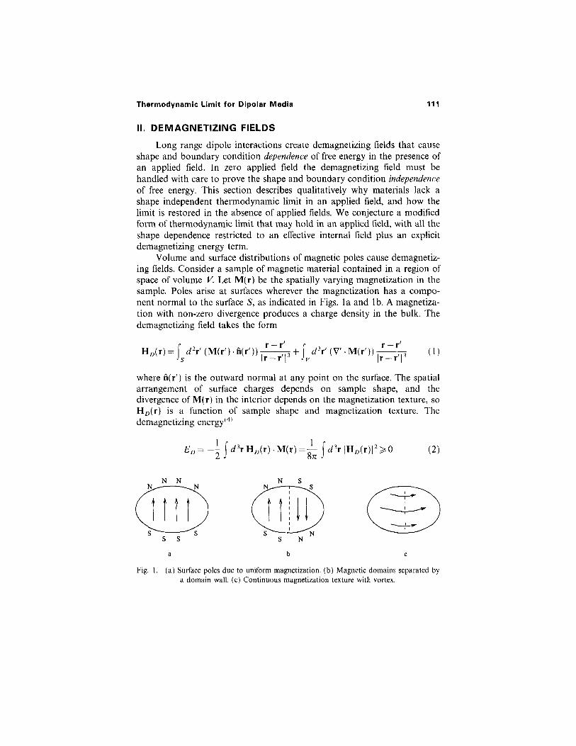
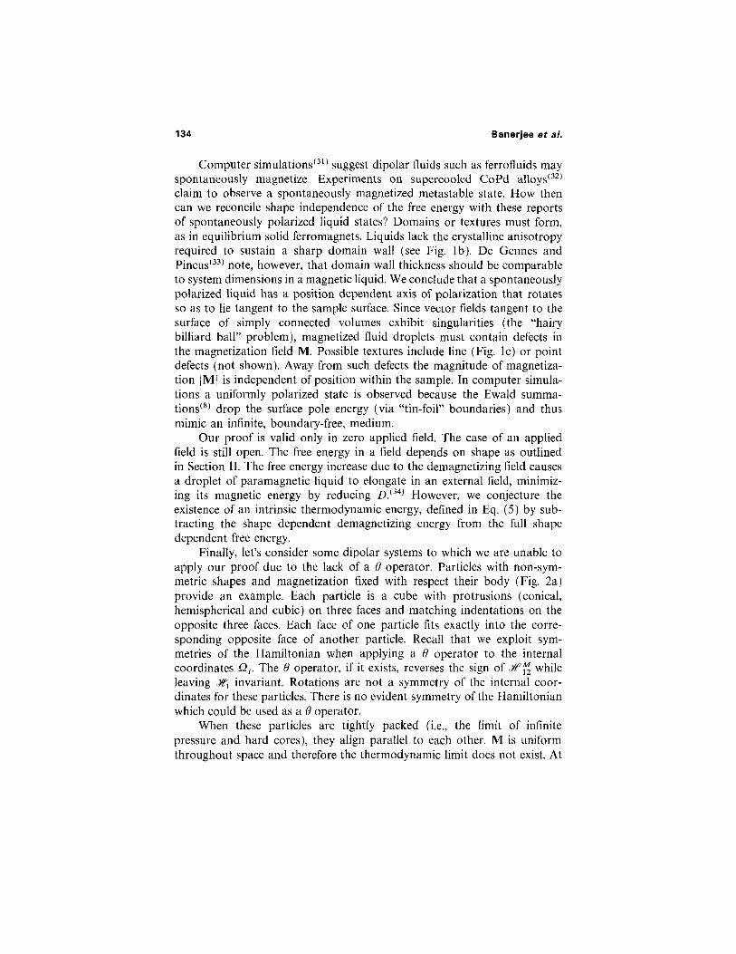
Fig. 1. (a) Surface poles due to uniform magnetization, (b) Magnetic domains separated bya domain wall, (c) Continuous magnetization texture with vortex.

where n(r') is the outward normal at any point on the surface. The spatialarrangement of surface charges depends on sample shape, and thedivergence of M(r) in the interior depends on the magnetization texture, soHD(r) is a function of sample shape and magnetization texture. Thedemagnetizing energy(4)

II. DEMAGNETIZING FIELDS

Long range dipole interactions create demagnetizing fields that causeshape and boundary condition dependence of free energy in the presence ofan applied field. In zero applied field the demagnetizing field must behandled with care to prove the shape and boundary condition independenceof free energy. This section describes qualitatively why materials lack ashape independent thermodynamic limit in an applied field, and how thelimit is restored in the absence of applied fields. We conjecture a modifiedform of thermodynamic limit that may hold in an applied field, with all theshape dependence restricted to an effective internal field plus an explicitdemagnetizing energy term.

Volume and surface distributions of magnetic poles cause demagnetiz-ing fields. Consider a sample of magnetic material contained in a region ofspace of volume V. Let M(r) be the spatially varying magnetization in thesample. Poles arise at surfaces wherever the magnetization has a compo-nent normal to the surface S, as indicated in Figs, 1a and 1b. A magnetiza-tion with non-zero divergence produces a charge density in the bulk. Thedemagnetizing field takes the form

Thermodynamic Limit for Dipolar Media 111

For highly elongated sample shapes, in the absence of demagnetizingeffects, we expect a thermodynamic limit for the free energy. Define fint(H0)as the free energy per unit volume of a system in the limit as total volumeF-> oo. The limit must be taken within ellipsoidal shapes for which thelength parallel to the field H0 grows faster than the orthogonal directions.Because there are no demagnetizing effects present, we call this free energydensity the intrinsic free energy density in a field.

A. Shape Dependence in a Field

When a system is placed in an external field H0, surface poles arisebecause the internal magnetization tends to align with the applied field.There are two important contributions to the resulting shape dependenceof the free energy. One is the explicit shape dependent energy (2), the otheris due to the shape dependence of the internal field

where the tensor D is the demagnetizing factor of the ellipsoid.(4) D is non-negative definite, and its trace equals 1. When the magnetization lies alonga principal axis of the ellipsoid, D is simply replaced by one of its eigen-values 0 < D < 1. For a magnetization parallel to a highly elongated needleshape, the demagnetizing factor D = 0 because the surface poles appearonly on the tips which are small and far removed from the bulk. Anotherspecial limit is that of magnetization normal to a flat pancake shape. Thisyields the maximum demagnetizing effect, since the surface poles appear ona large surface close to the bulk, so D = 1 in this case.

depends explicitly on the shape and magnetization texture of the systemthrough the demagnetizing field HD(r) .

In the special case of magnetization uniform throughout the sample,the demagnetizing field HD(r) comes only from the surface, because thedivergence term in Eq. (1) vanishes. However, HD(r) does not vanish asvolume increases at fixed shape. This is because the 1/r2 fall-off of the fieldfrom each surface charge is exactly offset by the r2 growth of surface area,and hence the number of surface charges. As a result, HD(r) is independentof the volume and the demagnetizing energy ED is extensive.

For the special case of a uniformly magnetized ellipsoid, HD, is con-stant within the ellipsoid and equals

112 Banerjee et al.

Note that the measured xshape has a maximum value equal to xint when H0

is parallel to the long axis of a highly prolate needle-shaped ellipsoid. Forany other geometry the demagnetizing effect reduces the measured suscep-tibility.

B. Shape Independence in Zero Field

Now consider a ferromagnetic material in zero applied field. If themagnetization were constant (Fig.1a), surface poles would create shapedependent demagnetizing fields and raise the energy as described in Eq. (2).A uniformly magnetized body lacks a shape independent thermodynamiclimit!

Alternative magnetization configurations reduce the demagnetizingenergy. One possibility (Fig. 1b) reverses magnetization in subregions sothat the fields from surface poles tend to cancel. Another possibility

where

Consider applying an external field H0 parallel to a principal axis of anellipsoidal sample. Because of the demagnetizing effect, the internal field His weaker than the applied field. Eliminating HD and H between Eqs. (3),(4), and (6) yields the shape dependent measured susceptibility

up to corrections that grow less rapidly than the volume. Equation (4)gives the internal field H and Eq. (2) gives ED.

Shape dependence of the free energy implies shape dependence of themeasured paramagnetic susceptibility. Assume that the magnetization M isrelated to the internal field H by an intrinsic (volume and shape indepen-dent) linear susceptibility xint according to

For more general shapes HD is non-zero, and may vary in space. Weconjecture that the shape dependent free energy Fshape may be expressed interms of the intrinsic free energy density as


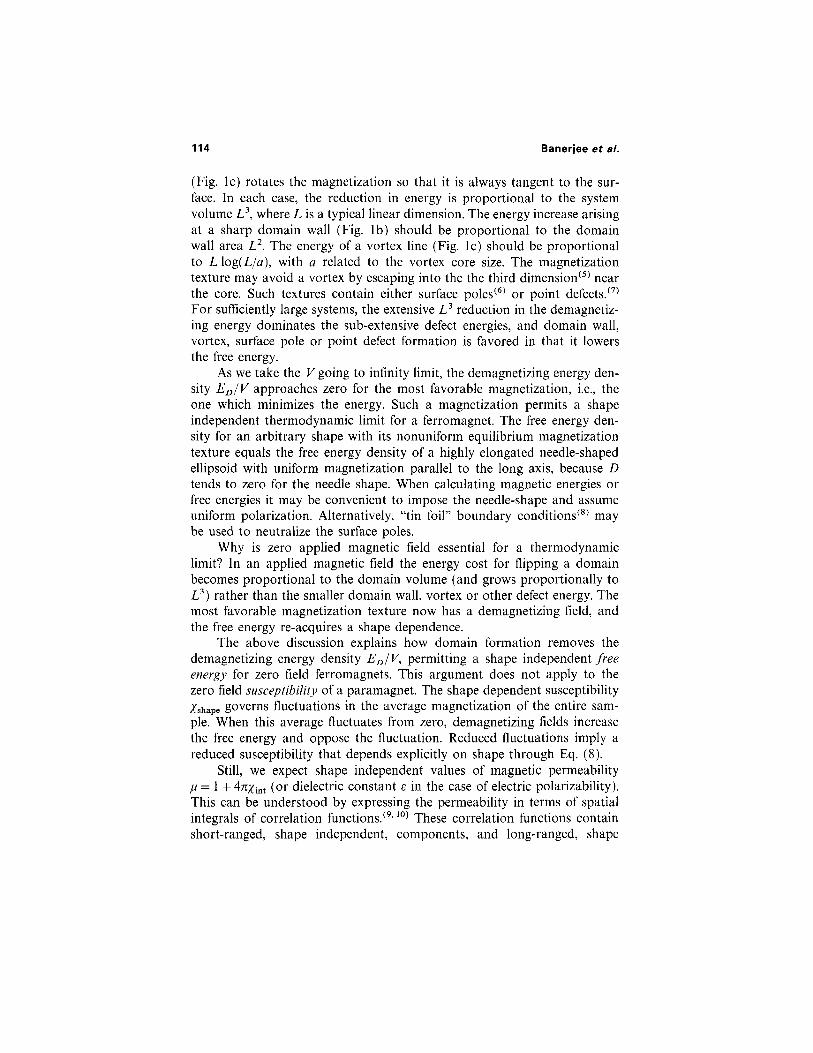
(Fig. 1c) rotates the magnetization so that it is always tangent to the sur-face. In each case, the reduction in energy is proportional to the systemvolume L3, where L is a typical linear dimension. The energy increase arisingat a sharp domain wall (Fig. 1b) should be proportional to the domainwall area L2. The energy of a vortex line (Fig. 1c) should be proportionalto L l o g ( L / a ) , with a related to the vortex core size. The magnetizationtexture may avoid a vortex by escaping into the the third dimension(5) nearthe core. Such textures contain either surface poles(6) or point defects.(7)

For sufficiently large systems, the extensive L3 reduction in the demagnetiz-ing energy dominates the sub-extensive defect energies, and domain wall,vortex, surface pole or point defect formation is favored in that it lowersthe free energy.

As we take the V going to infinity limit, the demagnetizing energy den-sity ED/V approaches zero for the most favorable magnetization, i.e., theone which minimizes the energy. Such a magnetization permits a shapeindependent thermodynamic limit for a ferromagnet. The free energy den-sity for an arbitrary shape with its nonuniform equilibrium magnetizationtexture equals the free energy density of a highly elongated needle-shapedellipsoid with uniform magnetization parallel to the long axis, because Dtends to zero for the needle shape. When calculating magnetic energies orfree energies it may be convenient to impose the needle-shape and assumeuniform polarization. Alternatively, "tin foil" boundary conditions(8) maybe used to neutralize the surface poles.

Why is zero applied magnetic field essential for a thermodynamiclimit? In an applied magnetic field the energy cost for flipping a domainbecomes proportional to the domain volume (and grows proportionally toL3) rather than the smaller domain wall, vortex or other defect energy. Themost favorable magnetization texture now has a demagnetizing field, andthe free energy re-acquires a shape dependence.

The above discussion explains how domain formation removes thedemagnetizing energy density ED/V, permitting a shape independent freeenergy for zero field ferromagnets. This argument does not apply to thezero field susceptibility of a paramagnet. The shape dependent susceptibility/shape governs fluctuations in the average magnetization of the entire sam-ple. When this average fluctuates from zero, demagnetizing fields increasethe free energy and oppose the fluctuation. Reduced fluctuations imply areduced susceptibility that depends explicitly on shape through Eq. (8).

Still, we expect shape independent values of magnetic permeabilityu = 1 +4nxint (or dielectric constant e in the case of electric polarizability).This can be understood by expressing the permeability in terms of spatialintegrals of correlation functions.(9,10) These correlation functions containshort-ranged, shape independent, components, and long-ranged, shape

114 Banerjee et al.

for N/V<pc where fL(p) is some finite valued function.

(2) Consider a system composed of two subsystems, 1 and 2, con-taining N1 and N2 particles, respectively. The particles in subsystem 1 areconfined in a region R1 with volume V1 and those in subsystem 2 are con-fined in a region R2 with volume V2. The two regions R1 and R2 areseparated by a distance of at least d from each other. Provided that d > d 0 ,for some fixed distance d0, the free energy of the system should satisfy anupper bound

A. Conditions on the Free Energy

Consider an N particle system contained in a region R of volume V.Taking the thermodynamic limit for the free energy means constructing asequence of sufficiently regular regions,(2) with increasing volume, so thatthe number of particles N divided by V approaches a definite value p as thevolume V tends to infinity. A limit is said to exist for the free energy densityif the free energy F divided by the system volume V approaches a limitingvalue F as the volume tends to infinity. The requirement of regularity(2)

prevents the regions R from getting too thin or constricted. We also intro-duce a model-dependent density pc that ensures the particles can fit intothe available volume when N/V is less than pc for sufficiently large finite N.

Two conditions on F suffice to prove the thermodynamic limit.

(1) The free energy F should satisfy the lower bound

dependent components. The permeability depends only on the short-ranged, shape independent, part of the correlation functions.

III. PROOF OF THE THERMODYNAMIC LIMIT

This section explains how we prove thermodynamic limits. First, westate required bounds on the free energy and explain how these bounds areused to prove the existence of a thermodynamic limit. Then, we show howto prove the necessary bounds on the free energy for classical systems whichare stable and tempered. These sections are rather brief and formal, andsimply review methods introduced previously.(1,2) Then, in Section IIIC weshow how to treat systems which include unstable and non-tempered dipoleinteractions.


The energy H is a function of particle center of mass positions ri, andinternal coordinates Qi. In the expression for Z, Q is the integral of dQi,over all its possible values. Internal coordinates depend on the type of par-ticle and may include orientation of the particle and direction ofmagnetization. For solids, particle center of mass positions and particleorientations are fixed, and the principal remaining variable is direction ofmagnetization.

We distinguish between two types of particle: superparamagnetic par-ticles,(12) for which the direction of magnetization rotates independently ofthe particle axes; normal particles, for which the direction of magnetizationis fixed relative to the particle axes. For normal particles, we do not includedirection of magnetization as an independent internal variable, because itis a function of particle orientation. In practice, superparamagnetic par-ticles exhibit a "blocking temperature" below which the direction ofmagnetization becomes locked to the particle axes, and the particlesbecome normal. In the specific models discussed below, we assume we arebelow the blocking temperature except where we explicitly invoke super-paramagnetism.

witn constants wB< oo and c > U .

These bounds suffice for proving the existence and shape independenceof the thermodynamic limit. Break an arbitrarily shaped system into manysmaller subsystems. The upper bound (10) bounds the total free energy interms of the subsystem free energies. Because the upper bound appliesregardless of the relative positions of the subsystems, provided d > d 0 , theoriginal system shape does not enter this bound on total free energy. Thelower bound (9) guarantees that the free energy density F/V reaches a finitelimit as the total volume K-> co with N/V- p. Because Fisher(2) explainsthis method in great generality, we need not reproduce his effort here.

B. Classical Stable and Tempered Systems

The free energy of a classical system of N identical particles in avolume V is F = — k3 T log Z, where Z is the partition function

where F1 and F2 are the free energies of subsystems 1 and 2 in isolationand(11)

116 Banerjee et al.

with A12 as defined in Eq. (11) , for d larger than some constant d0. Sub-stitute A12 for H2 in the total interaction energy (15) and evaluate thepartition function (12) to derive the upper bound (10) on F.

C. Dipolar Systems

The remainder of this paper considers systems whose Hamiltoniansinclude dipolar interactions in addition to stable, tempered interactions ofthe type described above. The dipole interaction, by itself, is neither stablenor tempered. In this section we explain how additional repulsive inter-actions may stabilize the system, and how the upper bound (10) may beproven despite the lack of tempering. The ideas introduced here are appliedto a wide variety of specific models in Section IV.

where H1 and H2 denote the energies of each system by itself, and H2 isthe interaction energy between the two subsystems. The upper bound holdsif the interaction H2 satisfies the weak tempering condition(11)

with COA < co a constant. Just substitute the lower bound (13) for H intothe partition function (12) to obtain the lower bound (9) on F, with thefunction

To prove the upper bound (10), consider the interaction of two sub-systems separated by distance d as described in Section IIIA. Write thetotal energy H in the form

Note the explicit dependence of Z on the system shape through thelimits of integration for the r, in Eq. (12). The free energy F inherits thisshape dependence. The conditions on F stated in Section IIIA guaranteethat the shape dependence is contained entirely in a sub-extensive term.Achieving the desired lower and upper bounds on free energy depends onproperties of the interaction energy jf. This section describes sufficientconditions to prove each bound.

The lower bound (9) holds for potentials that are stable in the sensethat


where vi and Vj are the regions of space occupied by the magnetic materialof particle i and j The magnetization distribution of the ith particle is M(r)for r inside vi, and for the jth particle is M(r') for r' inside Vj. Implicitly,HM depends on the particle center of mass positions and the particleorientations through vi and vj, the regions of space occupied by the par-ticles. For superparamagnetic particles, the direction of magnetization is aninternal coordinate for each particle, while for normal particles, themagnetization is determined by the particle orientation. Thus, HM is afunction of particle positions {r i} and internal coordinates {£ j}.

For the moment we consider only permanent magnetization(polarizable particles are discussed in Section IVC), and we assume themagnetized volumes of the particles are non-overlapping. The 1/r3

dependence of the magnetic interaction HM violates tempering because ofits slow decay at long range, and risks violating stability because of itsdivergence at short range.

We demand stability of the total interaction H to enforce the lowerbound (9) on the free energy. Because of the diverging short-rangemagnetic attraction, we need residual interactions that are sufficientlyrepulsive at short range to overcome the magnetic attraction. Hard-coreparticles, and soft-core particles with energies that diverge faster than 1/r3,satisfy this requirement, as we prove later in Section IV.

To achieve the upper bound (10) on the free energy we demand thatthe residual interaction HR be tempered and we exploit symmetries (if pre-sent) to handle the non-tempered magnetic interaction HM. Our strategylimits our proof to models possessing the required symmetries and temper-ing of residual interactions. Models lacking these characteristics may stillpossess a thermodynamic limit even though we cannot prove it. The sym-metries we require are broken by applied magnetic fields.

Consider two subsystems such that the N1 particles in region R1 areseparated by at least a distance d>d 0 >0 from the N2 particles in region R2.

The non-magnetic part of the interaction, HR, we call the residual inter-action. The magnetic interaction between the N particles takes the form(4)

Split the interaction energy H into two components:

Banerjee et al.118

Combining the bound (21) with the ensemble averages (23) and (24)proves the upper bound (10) on the fully interacting free energy F ( l ) .

To establish (24) we employ what we call a 9 operator, a map of thecoordinates of a system onto themselves in a one-to-one manner satisfyingthe following conditions. It leaves the center of mass position r, of eachparticle unchanged, it maps the internal coordinates i2i, onto themselves ina way which leaves the integration measure Oi=1 dui unchanged, and itleaves the Hamiltonian ,W invariant. In addition, when a system consists oftwo subsystems and 9 is applied to one but not the other, it reverses the

We will show that

Because the residual interaction HR is tempered, H 1 2 < z 1 2 . Its ensembleaverage, likewise, is bounded above:

where F(0) = F1+F2 is the free energy of the non-interacting subsystems,and the classical ensemble average of any quantity 3. takes the form

where the right side is a line tangent to the graph of F(A) at A = 0; hereF'(A) and F"(A) are the first and second derivatives. As a consequence, thefree energy F(1) of the fully interacting system satisfies the Gibbsinequality(31)

Let F(A) be the free energy of the combined system when the Hamiltonianis H1 + H2 plus a scaled interaction AH12. Because F(A) is a concave func-tion (that is, F"(A)<0), it is bounded above by

Let H1 and H2 be their respective Hamiltonians. Define the interactionenergy between the two subsystems by

119Thermodynamic Limit for Dipolar Media

The hard core interaction,

sign of the magnetic interaction H12Mbetween them. Specific models may ormay not possess such an operator. When a system is stable and possessesa 0 operator, we can obtain the desired upper and lower bounds on F toprove a thermodynamic limit.

If a 8 operator exists, it can be used to establish (24) in the followingway. Set J = H12 in (22), and consider the change of variables producedby applying the 9 operator to subsystem 1 but not subsystem 2. Thischange preserves the integration measure, but reverses the sign of theintegrand, since H1 and H2 are unaltered, but H12 changes sign. Conse-quently, the integral is equal to its negative, so it is zero.

IV. MODELS

Section III introduced a general strategy for proving thermodynamiclimits of permanently magnetized classical particles. The following sectionapplies that strategy to a variety of models. We start with identical hardcore particles, then treat dipolar soft spheres such as Stockmayer fluids. Wethen modify the proof to cover polarizable particles, and then treat quan-tum systems. Depending on the particular system, the greater challengemay lie in demonstrating the lower, or the upper, bound on F.

A. Identical Hard Core Particles

Consider a collection of TV identical, uniformly magnetized, hard corenormal particles of volume v, and fully contained within a region of spaceR of volume V. The magnetization M(r) is constant in magnitude for r involume vt of particle i and vanishes when r is not inside a particle. Insideparticle i the direction of M(r) = M, depends on the orientation Qi of theparticle. We require that the region M have a regular shape(2) and be largeenough so that all particles fit inside the region without overlapping. Thus,we restrict the number of particles so that the packing fraction 0 = Nv/V isnot too large. In particular, we assume a packing fraction <j>* >0 exists forwhich particles may be packed with any 0 < 0 < 0 * into any sufficientlylarge and regular volume.

Write the Hamiltonian as

120 Banerjee et al.

where H i D ( r ) is the field from magnetization M, of particle i with volume vi,obtained by substituting M,- for M(r) in Eq. (1) and integrating over thesurface and volume of particle i.

We use Eq. (29) to placer a lower bound on HM by a method similarto that of Griffiths.(3) For any magnetization distribution M(r) and thefield HD ( r ) caused by it

Here HD(t) is the field, due to all particles, defined in Eq. (1) and

for non-overlapping dipolar spheres with radius R, and dipole moment u,regardless of their positions and orientations. Because of the hard corerepulsion (26) we achieve stability (13) with wA=n2/2R3 for dipolar hardspheres (25). The lower bound on F follows as discussed in Section IIIB.We now generalize the proof of stability (13), and thus a lower bound on F,to particles of all shapes.

To prove stability we make use of the positivity of field energy. Addingthe magnetic self energy of each particle to HM gives the total energy ofthe whole system, considered as one magnetization distribution,

where ui, and ri are the dipole moment and position of the ith particle; ui,is the integral of M(r) over the volume of the ith particle; rij = ti, — Tj, andrij is the unit vector along rij.

The hard core interaction (26) by itself provides an example of a stableand tempered interaction. Since H H C > 0 , it obeys the stability condition(13) with wA = 0. Griffiths(3) proved the lower bound

prevents any overlap between particles. For non-overlapping configura-tions the magnetic interaction HM is as in (18). For the special case ofhard core spheres the expression (18) reduces to the simpler form


122

Hence

Banerjee et al.

Brown(4) rewrites the self energy in (30) as

where D,. is the demagnetizing tensor of an "equivalent ellipsoid;" it existsfor a particle of any shape, and k and / index the components of Di,- and M.Since Di is positive definite, with trace equal to 1,

Since all particles are identical, the magnetic interaction satisfies the lowerbound

Thus we confirm stability (13). The lower bound (9) on the free energyfollows with COA = 2nM2v.

For proving an upper bound on the free energy, notice that the hardcore interaction (26) is tempered, Eq. (16), with any d0>0. We identify thehard core interaction (26) as a residual interaction HR. The key to ourproof of an upper bound in Section IIIC was reversing the sign of themagnetic interaction energy H12, without changing H1, by applying anoperator 6 on subsystem 1. For particles with permanent magnetizationfixed relative to the particle, a rotation of each particle can reverse thedirection of magnetization. Such a rotation keeps the residual interactionsunchanged only if the particle shape has an axis of 2-fold symmetry per-pendicular to its magnetization. Hence at least one operator 9 exists, andour proof applies, for systems of identical particles with the required rota-tional symmetry in shape.

Some kinds of small particles, including many used in ferrofluids,(14)

exhibit superparamagnetism. Dipole moments rotate by Neel relaxation,(15)

or possibly quantum tunneling(16) without requiring rotation of the par-ticle itself. To describe the superparamagnetic classical particles, oneincludes in Qi, in addition to the Euler angles, a discrete variable Oi= ± 1specifying that the magnetization is parallel ( +1) or opposite ( — 1) to adirection fixed in the particle, and j dQi includes a sum over Oi. The 0operator is the map 0i,-> —O i , applied to every particle. For a quantum

Define a generalized mean

is a repulsive interaction with A > 0 and n > 3, and Hcoentral is any stable(13) and tempered (16) potential that is spherically symmetric. DefineH(n)

+ Hcentral to be the residual interaction HR. The upper bound (10)follows exactly as in Section IIIC because H(n) and Hcentral are both tem-pered and rotationally invariant. The proof of a lower bound (9) for suchsystems is more complicated than for hard core particles because there isno minimum distance of separation between the point dipoles.

To prove stability (13) and hence a lower bound (9), it suffices toprove that HM + H ( n ) is stable, since Hcentral is stable by assumption.Consider some configuration of a finite system of N particles. Let 2Ri bethe distance from the ith particle to its nearest neighbor. The magneticinteraction energy remains unchanged if each particle is replaced by asphere of radius Ri with uniform magnetization and the same dipolemoment \i. The self energy of such a sphere is [i2/2R3 . SinceHM + (ju2/2) En

=1 . R - 3 > 0 by positivity of field energy (see discussion inSection IVA), and H ( n ) > ( A / 2 } £n

=1 (2R i)- n , we write

where HM is the point dipole interaction (21),

particle, the corresponding operation is time reversal applied to the par-ticle's magnetization. In either case, the 6 operator has the propertiesspecified in Section IIIC, so the argument given there shows that anysystem of hard core superparamagnetic particles, with any shape of par-ticle, has a thermodynamic limit.

B. Dipolar Systems with Central Forces

Consider a system of particles interacting with Hamiltonian


The Hamiltonian in (45) is special case of our model (36). The Stockmayerfluid(18) is the case with n = 12, w = 6, and hence will also have a shapeindependent thermodynamic limit. Dipolar soft spheres(19) are the trivialcase C = 0 and .Wcentral = 0.

Ruelle(1) showed that generalized Lennard-Jones potentials with B, C>0and n>m>3 are stable. To demonstrate stability including the dipoleinteraction, divide the repulsive term into two positive pieces, B = A + B'.Attribute B' to a new (but still stable) Lennard-Jones potential and use theremainder A to define the repulsive potential H(n),

where the Lennard-Jones potential is

Our model (36) is therefore stable.Let's apply this general proof to some special cases. Our proof applies

to generalized Lennard-Jones particles with dipole interactions. TheHamiltonian for such a system is

where X=(1/N)Ei=1 R-3. The bound (41) for HM + H(n) has a mini-mum because n > 3 and A > 0. In particular

for n > 3. Combining Eq. (40) with Eq. (38) we write

Using the property that G(t) increases monotonically for positive t ( l 7 ) wefind

124 Banerjee et al.

The model fails because of its assumed induced point dipole. The pointdipole applies rigorously only to an infinitesimal volume. However, thepolarizability a necessarily vanishes in the limit of zero volume, due to theself-induced demagnetizing field. Finite size particles can have oc^O.However, the DID model omits multipole moments due to the spatialvariation of fields and magnetization inside the particles. Higher order mul-tipole interactions between particles become important when the particlesapproach each other,(21,22) and are required for stability.

Consequently, we work with a more physically realistic model.(20) Byincorporating the full magnetic interaction (dipole and higher moments)and the spatial variation of fields within a particle, our model satisfiesstability in general. This model represents the polarizability of atoms andmolecules more accurately than the DID model. Each particle has a perma-nent magnetization density which is constant in the interior of the particle,but whose direction is determined by the orientation of the particle. (Forexample, imagine that the particles are prolate ellipsoids with magnetiza-tion along the long axis.) The particles are "hard," so that their volumescannot overlap. Consequently, the permanent magnetization is a vectorfield Mp(r), equal to zero unless r is inside some particle, where it takes ona value whose magnitude is independent of the particle but whose directionis tied to the particle's orientation Q.

In addition, each particle contains linearly polarizable material givingrise to an induced magnetization


C. Polarizable Particles

Consider a system of identical hard core particles that contain perma-nent magnetic moments but are further linearly (i.e., proportionally to thelocal field) polarizable. The simplest model for such systems is the dipole-induced-dipole (DID) model.(10,20) The model consists of spherical par-ticles with a point dipole moment at the center, and with the inducedpolarization an additional point dipole moment of strength aH. This modellacks stability in general. For example, with two spherical particles ofpolarizability a and hard core radius R, stability is lost when

where H(r) is the total magnetic field at r, and the susceptibility tensor x(r)is zero unless r is inside some particle, where its value is independent of rbut tied to the orientation of the particle: that is the principal values of x,

equals the work done bringing initially isolated polarizable particles intointeraction with each other.

The stability (13) and hence the lower bound (9) for this systemfollows from the positivity of field energy. Rewrite the magnetic energy inEq. (49) as (see Appendix A for details)

The first term is the demagnetization energy (2) of the permanentmagnetization distribution, and the second term represents the work donein introducing linearly polarizable material into this permanent field.Evaluating (49) for an isolated particle defines the self energy Ese l f per par-ticle. The difference

where Hp(r) is the field from permanent magnetization density Mp, and isgiven by (1) with M set equal to Mp, whereas H i(r) is due to the inducedmagnetization: in (1) set M equal to Mi. Note that even an isolated particlewill have an induced magnetization because the demagnetizing effect willgive rise to a non-zero Hp, and the total H inside the particle must bedetermined self-consistently, as it both induces a magnetization, (47), andis partly (Hi) determined by that magnetization.

Because of this requirement of consistency between total field andmagnetization, the magnetic interaction of polarizable particles is a multi-body interaction, and is much more complicated than the pairwise multipoleinteractions of permanently magnetized particles discussed in Section IVA.To write down the interaction energy HM of a configuration of polarizableparticles, it is convenient to calculate the work done assembling the con-figuration, starting with the particles well separated from each other atinfinity. For any arrangement of particles, the total magnetic energy is

and the relationship of the principal axes of X to the orientation of theparticle, are same for every particle.

The total magnetic field H(r) in (47) is

126 Banerjee et al.

Here H = Z i=1 p2, /2m is the kinetic energy operator. The exchange inter-action(23) is H E X = 1 Z i j J ( r i j ) S i - S j , where S,- is the spin operator for par-ticle i, rij is the distance between particles i and j, the couplings J(rij) areassumed to satisfy conditions consistent with stability, and the sum is overall i=j . The dipole interaction HM is given by (27) with dipole momentsHi= gS i . The residual interaction HR may be any stable and tempered

which is sufficient to prove the upper bound on F, as discussed inSection IIIC.

D. Quantum Systems

Our proofs extend to quantum systems. Consider a system of N identi-cal spin S particles in volume V, which may obey Boltzmann, Fermi-Diracor Bose-Einstein statistics. The Hamiltonian is

where C12 is odd under reversal of the permanent magnetization of par-ticles in subsystem 1 by the 6 operator, and N12<0. Since 012 is odd, itsensemble average vanishes. Then

where H1 and H2 are the magnetic interaction Hamiltonians for the sub-systems by themselves; i.e., H1 is the energy of subsystem 1 with sub-system 2 placed infinitely far away. We show in Appendix B that, forpositive-definite X,

The stability and lower bound then follow as in the case of identical hardcore particles.

To prove the upper bound (10), consider two subsystems 1 and 2separated by a distance d>d 0 >0 as in Section III A. Write the interactionHamiltonian between these two subsystems as

Since 1 +4?rx is positive definite, Hrt>0, hence


It will also be convenient to define a scaled Hamiltonian

To begin with, we assume that the N1 particles with labels in I1 areconfined to a region of space R1 c: R with volume V1, while theN2 = N — N 1 particles with labels in I2 are confined to a region R2C R ofvolume F2, and that the minimum separation of R1 and R2 is a distance

where H1includes all terms in (56) (one particle, two-particle, etc.) involv-ing only particles in the set i1 with labels 1, 2,..., N1, $f2 includes the termsinvolving only particles in the set L2 with labels N1 + 1, N1 +2,..., A1 + N2,and H12 all the remaining terms. The interaction energy H12 is a sum ofmagnetic dipole, exchange, and residual terms

where the trace Tr is carried out over states of appropriate symmetry withrespect to interchange of particles. For Boltzmann particles C = N! and forfermions and bosons C= 1. The free energy F is —kBT log Z.

The stability of 3?, in the sense that its spectrum has a lower boundproportional to N, see (13), follows from the positivity of Jf (no negativeeigenvalues) and the stability of JfM + 3fEX + 2fR. Lower bounds onclassical energies of the sort derived in Sections IVA and IVB are easilyextended to operator inequalities which demonstrate the stability of3CM +2FR. That this stability is preserved upon adding 3fEX requires asuitable choice of J(r). For example, in the case of hard core particles itsuffices that J(r) be bounded and decrease more rapidly than r~ 3 ~ 6 forsome e > 0.

We now address the upper bound on the free energy. Write theHamiltonian in the form

interaction that remains unchanged under simultaneous spin reversal of allparticles, such as the hard core or central force interactions discussed inSections IVA and IVB. Implicit in our definition of the Hamiltonian is theconfinement of particles in a region 8% of volume V with hard wall bound-ary conditions. The partition function is

128 Banerjee et al.

where D = N1! N2! for Boltzmann particles and D = 1 for fermions andbosons. If this partition function is evaluated using 3? with A = 0 in (60),—k^T times its logarithm is the sum F 1+F 2 of free energies for theseparate systems of particles in regions R1, and R2, each evaluated as if theother region did not exist, since the interactions between the two sets ofparticles have been "turned off."

An upper bound on the free energy F of the full system of N particlesconfined to region ffl, in the form of the Eq. (10) is obtained through thefollowing steps.

(1) "Turn on" the interaction between the particles in regions Rl andR2 by letting A increase from 0 to 1. The resulting free energy is denotedby FN1,N2. The superscript <& indicates that particles are confined to regionsR1 and R2.

(2) Remove the constraint that only particles in set u1 are found inR1 and only those in set I2 are found in R2 . Any particle may be anywherein the union of R1 and R2, provided there are exactly Nr particles in R1

and N2 particles in R2. This involves introducing appropriately sym-metrized wavefunctions.

(3) Relax the constraint that precisely N1 particles are in R1 and N2

in R2. We still require that there be a total of N particles in the union ofR1 and R2.

(4) Relax the constraint that the particles lie in either R1 or R2, sothat all particles can be anywhere in the larger region R.

Since steps 2, 3, and 4 do not require special attention to long rangeinteractions, they are discussed in Appendix C. Basically, each time a

where the integer arguments are particle labels. The {| < / > m > } form a com-plete set of states for the N1 particles in R1, with appropriate symmetryunder interchange of particles and {|xn>>} is a similar set for the N2 par-ticles in R2. The product states (61) have no symmetry for the interchangeof particles between the two sets R1 and R2, as indicated by the superscripttfl. Due to this lack of symmetry the partition function is given by

d>d 0 . Note that (in general) R is larger than R1 u R2. The Hilbert spaceof this system is spanned by product states of the form


for 1 <i<N1, and HM12 is a sum of pairwise products of spin operators,one from the collection L1 and one from L2. Thus <H12)/l = 0 is equal toits negative and vanishes. The same argument applies to < H 1 2 > i = 0 .

Consequently, after following the remaining steps 2, 3, and 4 con-tained in Appendix C, we have a bound corresponding to (10) in the classi-cal case. This bound together with that in (9), which (as already noted)follows from the stability of 3f, completes the proof of the existence of athermodynamic limit in the quantum case, see Section IIIA.

It is possible to treat the translation degrees of freedom classically andthe spin quantum mechanically. The proof of a thermodynamic limit for

because

The third term in (64) is bounded by the upper bound A12 on H12. Thefirst and second terms vanish for the following reason. Let 0 be the anti-unitary spin reversal operator which reverses all the spins of the particlesin collection ,91. It is a symmetry of H1, because H1m and H1ex involveproducts of two spin operators and H1Ris, by assumption, invariant underthe reversal of all spins. Consequently, if the { |<^m>} are the eigenstates ofH1, the states 0 \<j>my = |^m> are also eigenstates with the same eigenvalues.In evaluating the trace in the numerator of (65) we can employ a completeset {\<t>my !/„>}, where the {|xn>} are the eigenstates of H2, or, equiv-alently, {|^m> |/n>}. However,

where the averages are with respect to Boltzmann weights with A = 0. Forexample

which is known as the Bogoliubov inequality.(13) The first term on the rightis F1 + F2, and the second is

constraint is relaxed the free energy decreases, except for step 2, where itremains constant. Thus the upper bound obtained for FN1,N2 applies to F.

For step 1 we use the fact that FN1,N2 is a concave function of A, andtherefore

130 Banerjee et al.

such a "semi quantum" model is similar to the "fully quantum" treatment.The averages of H12M and H12EX involve sums over all spin states andintegrals over all particle positions. Using the spin reversal operator 9,introduced earlier in this section, and doing the sums over all spin statesfirst, one sees that the average values of H12M and H12EX vanish. The residualinteractions H12R are bounded by d12, and therefore our proof goesthrough.

One may define another "semi quantum" model of classical spins andclassical dipoles with center-of-mass motion of the particles treated quan-tum mechanically. The averages of H12 and H12 contain integrals over allspin orientations and sums over all spatial wavefunctions in this case. Theproof is similar to that of classical particles. Doing the integrals over par-ticle spins first, gives zero for the average of H12 + H12, because they areboth odd with respect to spin reversal. The sum over the spatial wavefunc-tions then yields the desired upper bound on < H 1 2 ) ^ = 0 and our proof goesthrough. We can even include classical polarizability (Section IVC) in sucha model. In this case the average of H12 is non positive, and again we getthe required upper bound (10) on the free energy.

V. ELECTRIC POLARIZATION

So far we phrased our discussion entirely in terms of magnetic inter-actions. However our proof applies to many electrically polarized orpolarizable materials as well. Electric fields E and D fields satisfy the sameMaxwell equations as magnetic fields H and B, respectively, provided nofree charges and currents are present. By replacing fields H, B andmagnetization M with fields E, D and polarization P, respectively, ourproofs run exactly as for magnetic materials. We assume stability, temper-ing of the residual interactions, and the existence of a 9 operator. Thus weprove the existence of a shape independent thermodynamic limit for theelectric analogue of each of the classical models discussed in Sections IV.

For ferroelectric identical hard core particles, use the Hamiltonian


where dPp is the electric Interaction between particles. The proof followsSection IVA with the replacement of fields discussed at the beginning ofthis section. For electric dipolar systems with central forces the interactionHamiltonian is

between any two water molecules m, n, where / and j run over the chargesqt and qt, respectively, on molecule m and n, ry is the separation betweencharges and r00 is the separation between oxygen ions. For the abovemodel there is no symmetry operation available which can reverse all theelectric interactions while keeping the residual (Lennard-Jones) interac-tions unchanged. A 9 operator therefore does not exist for this model andwe cannot apply our proof. We suppose that our qualitative argument(Section IIB) demonstrating existence of a shape independent thermo-

The proof goes through as in Section IVB, with the existence of a shapeindependent thermodynamic limit for electric dipolar soft spheres andStockmayer fluids as special cases. For electrically polarizable hard coreparticles, H = Hp + HHC where Hp, the electric interaction betweenpolarizable particles, is defined analogously with ,HM in Eq. (50). After thereplacements of fields and magnetization discussed at the beginning of thissection, the proof proceeds as in Section IVC. Quantum models can betreated as discussed in Section IVD.

Adding another layer of complexity, we may define models combiningfeatures of electric and magnetic models already discussed. The possiblevariations are too numerous to describe individually. We simply note herethat stability including only magnetic or only electric interactions ensuresstability with the two added together. Finding a 0 operator may be moredifficult. For example, a 180° rotation axis must lie perpendicular to bothM and P.

For the crude dipolar particle models discussed above, the electric andmagnetic problems are fully equivalent. For applications to realistic modelsof specific materials, however, it is generally harder to find a 0 operator inthe case of electric materials. The analogue of time reversal (which providesa 0 operator for superparamagnetic particles) is charge conjugation. Thishas the undesirable effect of turning matter into antimatter! Without a 0operator we cannot apply our proof.

For an example of a model outside our proof, consider a fluid of H2Omolecules (water). Modeled as a dipolar hard sphere or a Stockmayer fluidthe thermodynamic limit follows from our discussions above using rotationas the 6 operator. Real H2O molecules lack this rotational symmetry. Forexample, the TIPS 3 site model of water'24' places positive charges on thehydrogens and a negative charge on oxygen. Coulomb interactions betweenall intermolecular pairs of charges, and a Lennard-Jones interactionbetween the oxygen atoms, gives the interaction

132 Banerjee et al.

dynamic limit based on domain formation still holds, but for technicalreasons we cannot prove it.

Yet another example is provided by models of ferroelectric materialswith mobile charges. Charges transfer among dissimilar chemical elements,so no d operator is likely to exist. Furthermore, the definition of polariza-tion becomes ambiguous, depending on how the unit cell is defined in thecase of a crystal,(25) or on the surface charge for non-crystalline materials.The question of appropriate thermodynamic limits for model ferroelectricswith mobile charges remains under discussion.(26)

For models containing only bound charges, our qualitative argument(Section IIB) suggests the equilibrium state has no depolarizing energydensity. When the microscopic coulomb charges are taken into account,including the possibility of molecular dissociation and the Fermi statisticsof the constituent particles, the problem falls into the class of materials forwhich Lieb(27) proved a thermodynamic limit. Free electric charges screenthe 1/r Coulomb potential, restoring the thermodynamic limit.

VI. CONCLUSIONS

We proved the existence and shape independence of the free energydensity for a variety of dipolar systems. Three essential conditions wereidentified: stability, tempering of residual interactions, and the existence ofa 0 operator that commutes with H1,H2 and H12 while reversing the signof H12. Our proof covers systems of identical hard core particles withuniform permanent magnetization. We also treat dipolar soft spheres andStockmayer fluids, systems with magnetizable or polarizable material, andwe consider electric as well as magnetic dipoles. Except for the case ofsuper-paramagnetic particles, the existence of a 0 operator requires sym-metries such as a 2-fold axis of rotational symmetry perpendicular to themagnetization/polarization of each particle.

Having proven shape independence of the free energy we now considersome implications of the proof. For the systems covered by our proof, ther-modynamic states and phase diagrams do not depend on size or shape.(28)

Intrinsic thermodynamic quantities such as pressure and chemical potentialare independent of sample shape and position within a sample. Whencalculating free energies of magnetized states, care must be taken to removethe depolarizing field if uniform magnetization is assumed. Failure to do soleads to either boundary-condition or shape dependence of thermodynamicproperties.(26,28-30) Two convenient ways to remove the demagnetizingfields are to study highly prolate ellipsoids or to use tin-foil boundary con-ditions(8)


Computer simulations(31) suggest dipolar fluids such as ferrofluids mayspontaneously magnetize. Experiments on supercooled CoPd alloys(32)

claim to observe a spontaneously magnetized metastable state. How thencan we reconcile shape independence of the free energy with these reportsof spontaneously polarized liquid states? Domains or textures must form,as in equilibrium solid ferromagnets. Liquids lack the crystalline anisotropyrequired to sustain a sharp domain wall (see Fig. Ib). De Gennes andPincus'33' note, however, that domain wall thickness should be comparableto system dimensions in a magnetic liquid. We conclude that a spontaneouslypolarized liquid has a position dependent axis of polarization that rotatesso as to lie tangent to the sample surface. Since vector fields tangent to thesurface of simply connected volumes exhibit singularities (the "hairybilliard ball" problem), magnetized fluid droplets must contain defects inthe magnetization field M. Possible textures include line (Fig. 1c) or pointdefects (not shown). Away from such defects the magnitude of magnetiza-tion |M| is independent of position within the sample. In computer simula-tions a uniformly polarized state is observed because the Ewald summa-tions(8) drop the surface pole energy (via "tin-foil" boundaries) and thusmimic an infinite, boundary-free, medium.

Our proof is valid only in zero applied field. The case of an appliedfield is still open. The free energy in a field depends on shape as outlinedin Section II. The free energy increase due to the demagnetizing field causesa droplet of paramagnetic liquid to elongate in an external field, minimiz-ing its magnetic energy by reducing D.(34) However, we conjecture theexistence of an intrinsic thermodynamic energy, defined in Eq. (5) by sub-tracting the shape dependent demagnetizing energy from the full shapedependent free energy.

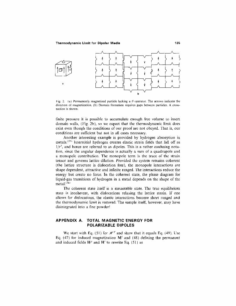
Finally, let's consider some dipolar systems to which we are unable toapply our proof due to the lack of a 6 operator. Particles with non-sym-metric shapes and magnetization fixed with respect their body (Fig. 2a)provide an example. Each particle is a cube with protrusions (conical,hemispherical and cubic) on three faces and matching indentations on theopposite three faces. Each face of one particle fits exactly into the corre-sponding opposite face of another particle. Recall that we exploit sym-metries of the Hamiltonian when applying a 9 operator to the internalcoordinates £ i , . The 9 operator, if it exists, reverses the sign of H12 whileleaving H1 invariant. Rotations are not a symmetry of the internal coor-dinates for these particles. There is no evident symmetry of the Hamiltonianwhich could be used as a 9 operator.

When these particles are tightly packed (i.e., the limit of infinitepressure and hard cores), they align parallel to each other. M is uniformthroughout space and therefore the thermodynamic limit does not exist. At

134 Banerjee et al.


Fig. 2. (a) Permanently magnetized particle lacking a 0 operator. The arrows indicate thedirection of magnetization, (b) Domain formation requires gaps between particles. A cross-section is shown.

finite pressure it is possible to accumulate enough free volume to insertdomain walls, (Fig. 2b), so we expect that the thermodynamic limit doesexist even though the conditions of our proof are not obeyed. That is, ourconditions are sufficient but not in all cases necessary.

Another interesting example is provided by hydrogen absorption inmetals.(35) Interstitial hydrogen creates elastic strain fields that fall off asl/r3 and hence are referred to as dipoles. This is a rather confusing nota-tion, since the angular dependence is actually a sum of a quadrupole anda monopole contribution. The monopole term is the trace of the straintensor and governs lattice dilation. Provided the system remains coherent(the lattice structure is dislocation free), the monopole interactions areshape dependent, attractive and infinite ranged. The interactions reduce theenergy but create no force. In the coherent state, the phase diagram forliquid-gas transitions of hydrogen in a metal depends on the shape of themetal.(36)

The coherent state itself is a metastable state. The true equilibriumstate is incoherent, with dislocations relaxing the lattice strain. If oneallows for dislocations, the elastic interactions become short ranged andthe thermodynamic limit is restored. The sample itself, however, may havedisintegrated into a fine powder!

We start with Eq. (51) for ,HT and show that it equals Eq. (49). UseEq. (47) for induced magnetization M' and (48) defining the permanentand induced fields Hp and Hi to rewrite Eq. (51) as

APPENDIX A. TOTAL MAGNETIC ENERGY FORPOLARIZABLE DIPOLES

where M1(r) is the induced magnetization which would be present in sub-system 1 were subsystem 2 absent, and M2(r) that of subsystem 2 were sub-system 1 absent.

Using Eqs. (A3) and (A4) to simplify Eq. (A1) gives Eq. (49), provingequality of our expressions (49) and (51) for HT.

APPENDIX B. INTERACTION ENERGY BETWEEN TWOSUBSYSTEMS OF POLARIZABLE DIPOLES

Let Hp1(r) and Hp2(r) be the fields due to the permanent polarizationin subsystems 1 and 2 located in non-overlapping regions H1 and H2. Theinduced magnetizations in the two subsystems can be written in the form

Since Eq. (A2) holds for any two arbitrary magnetization distributions, weset M1 = M2 equal to the induced magnetization M'. Then Eq. (A2) gives

Similarly, setting M1= Mp and M2 = Mi in Eq. (A2) gives

For any two magnetization distributions M1(r), and M2(r) and the fieldsH1(r)and H2(r) caused by them respectively, the following identityholds:(4)

136 Banerjee et al.

because the interaction-induced magnetization M' has lower energy thanthe isolated self-magnetization Ms. Upon replacing M} in (B4), withM i - M s , ( B l ) , one sees that (B5) implies that

APPENDIX C. QUANTUM SYSTEMS

Here are the details for steps 2, 3, and 4 in Section IVD. For step 2note that the formal Hamiltonian H(A=1), defined in Eq. (60), is sym-metrical under the interchange of any two particles, since the right side of

is non-positive as we now show. A theorem by Brown(4) states that for aparamagnetic polarizable material in an applied field, the unique inducedmagnetization Mi given by Eq. (47) minimizes the total magnetic energy.Applying that theorem to our system we observe that

is odd under reversal of the permanent magnetization of particles in sub-system 1 by the 0 operator, and

Break H12 into odd and non-positive components H12 = H12 + H12,where

Using Eqs. (49) for .WT and (50) for HM to find the interactionHamiltonians H1, H2 and HM for the two subsystems and the wholesystem, respectively, we write the interaction energy in (53) as


note that factors 8mm,, dnn, follow from orthonormality of the single particlestates in (C1). To get the factor dpp- consider p ^ p' both belonging to &.There is at least one particle / which is in R1 under P, and in R2 under p'.

(58) is simply a way of segregating terms in the sum representing H. Toallow any particle to be anywhere in R1, u R2, subject to the requirementof N1 particles in R1 and N2 in R2, replace the Hilbert space of the form(61) with another spanned by states with appropriate symmetries underinterchanging of any pair of particles. We now construct such a Hilbertspace for each type of statistics as indicated by Fisher.(2)

First consider identical particles obeying Boltzmann statistics and let{l« y >}> .7 = 1,2... be a complete orthonormal set of single particle states(including spin) for a particle confined to R1.A basis {|$m» for the par-ticles with labels in ff[ can then be written in the form

138 Banerjee et al.

where the operator ap applies permutation p to the Nl + N2 arguments.The set {IV'm,«,/,)} for m and n defined previously, and p belonging to SP,forms an orthonormal basis for the N particles in R1^R2, allowing anyparticle to be in either region, subject to the constraint of NI particles in^?! and the remaining N2 in R2.

To prove orthonormality,

It is clear that & contains P = N\/(N1! V2!) permutations, one for eachway of partitioning the integers from 1 to N into two collections one con-taining N1 and the other containing N2 integers. Then define states

where m stands for the sequence (ml,m2...mNi) of integer labels. In thesame way, a basis {|#B>} for particles with labels in £f2 can be constructedusing single particle states {|v*>|, k= 1, 2... for a particle confined to ^2.

To construct a basis in which any NI particles are in R1and any N2

particles in 3%2. we proceed as follows. Consider the collection 3? of per-mutations p of the integers (1, 2...N), where p(j) is the image ofy under p,with the property that

Only terms with p = p' survive because of (C5). Since ( ± }2n(p) = 1, the restof the proof is similar to the Boltzmann case.

where n(p] is 0 for an even and 1 for an odd permutation /?, and \(j>my and!/„> are assumed to have appropriate symmetry with respect to inter-change of particles withinR1 and within R2,respectively. We use the setof states {|i/'m,«)} to evaluate the trace in the partition function (57):

which is the same as the partition function ZN1,N2 (defined in Eq. (62))evaluated in the Hilbert space spanned by { | i A m , n } . The free energyFN1,n2 therefore is equal to FN1,N2.

For fermions (—) and bosons (+) the appropriately symmetrizedorthonormal states are

The Hamiltonian, being symmetric, commutes with ap. The sum over ptherefore just gives a factor of P, so that

because the Hamiltonian does not interchange particles between the tworegions R1 and R2.

We can use the set of states { \ \ l / m , n , p > } to evaluate the trace in thepartition function (57)

The inner product (C4) contains a factor <//"'(/>(/)) I v" ' ( /> ' ( / ) )> thatvanishes because the \/uJy vanish outside $?,, the |vfc> vanish outside J?2-Recall that R1 and R2 do not overlap. Finally, the normalization conditionin (C4) follows from the unitarity of ap. In addition note that for p + p'both belonging to &,


ACKNOWLEDGMENTS

We acknowledge useful discussions with H. Zhang, Ralf Petscheck,J. J. Weis and D. Levesque. This work was supported by NSF grant DMR-9221596 and by the A.P. Sloan foundation.

REFERENCES

1. D. Ruelle, HeIv. Phys. Acta 36:183 (1963); D. Ruelle, Statistical Mechanics (W. A. Benjamin,Inc. 1969).

2. M. E. Fisher, Arch. Rat. Mech. Anal. 17:377 (1964).

where {|0/>} is any orthonormal set of states. Choose {|0/>} to be the setof energy eigenstates {|i/'m>} of Jf in R1 u R2. It follows that the partitionfunction Z for region R, is greater than Z* for R1 u R2, and thus

Step 4 in Section IVD exploits the fact that region R containsR1 u R2 . Whenever particles are allowed to move in a larger region, thepartition function goes up and the free energy goes down. The quantumversion of this result is based on the fact that an energy eigenstate |i^m> ofJf in the smaller region, with energy Em, belongs to the Hilbert space ofthe larger region. Although it is not an eigenstate of 3P in the larger region,it is still the case that

Now we make use of Peierl's theorem, which states that

where ZN1,N2 is the partition function for N1 particles in R1 and N2 par-ticles in R2 . Consequently Ze is not smaller than ZN1,N2 for any particularN1 and N2 = N-Nlt and

Step 3 in Section IVD follows from the observation that the partitionfunction Z^ for N particles in R1 u R2 is & sum of positive terms of theform

140 Banerjee et al.

3. R. B. Griffiths, Phys. Rev. 176:655 (1968).4. W. F. Brown, Magnetostatic Principles in Ferromagnetism (North-Holland, Amsterdam,

1962).5. N. D. Mermin, Rev. Mod. Phys. 51:591 (1979).6. A. Ahroni and J. P. Jakubovics, IEEE Trans. Magn. 32:4463 (1996).7. B. Groh and S. Dietrich, Phys. Rev. Lett. 79:749 (1997).8. S. de Leeuw, J. Perram, and E. Smith, Ann. Rev. Chem. 37:245 (1986).9. J. M. Deutch, Ann. Rev. Phys. Chem. 24:301 (1973).

10. M. S. Wertheim, Ann. Rev. Phys. Chem. 30:471 (1979).11. Fisher(2) defined tempering with the stronger condition H 1 2 < N l N 2 w B / S 3 + e , but the

weaker condition employed in Eq. (16) suffices.12. C. P. Bean, 7. Appl. Phys. 26:1381 (1955).13. H. Falk, Am. J. Phys. 38:858 (1970).14. R. E. Rosensweig, Ferrohydrodynamics (Cambridge, 1985).15. W. Luo, S. R. Nagel, T. F. Rosenbaum, and R. E. Rosensweig, Phys. Rev. Lett. 67:2721

(1991).16. D. D. Awschalom, et al., Phys. Rev. Lett. 68:3092 (1992).17. M. Abramowitz and 1. A. Stegun, Handbook of Mathematical Functions with Formulas,

Graphs and Tables (Dover, 1965), Section 3.2; G. H. Hardy, J. E. Littlewood, andG. Polya, Inequalities (Cambridge University Press, 1964), p. 26.

18. M. J. Stevens and G. S. Grest, Phys. Rev. E 51:5976 (1995).19. D. Wei and G. N. Patey, Phys. Rev. A 46:7783 (1992).20. D. W. Oxtoby, Chem. Phys. 69:1184 (1978).21. G. N. Patey and J. P. Valleau, J. Chem. Phys. 64:170 (1976).22. M. Widom and H. Zhang, Phys. Rev. £51:2099 (1995).23. N. W. Ashcroft and N. D. Mermin, Solid State Physics (Rinehart and Winston, 1976).24. W. L. Jorgensen, J. Am. Chem. Soc. 103:335 (1981).25. D. Vanderbilt and R. D. King-Smith, Phys. Rev. B 48:4442 (1993).26. X. Gonze, Ph. Ghosez, and R. W. Godby, Phys. Rev. Lett. 78:294 (1997).27. E. H. Lieb, Rev. Mod. Phys. 48:553 (1976).28. In this regard see B. Groh and S. Dietrich, Phys. Rev. Lett. 72:2422 (1994), a comment

by M. Widom and H. Zhang, Phys. Rev. Lett. 74:2616 (1995), and a response by B. Grohand S. Dietrich, Phys. Rev. Lett. 74:2617 (1995).

29. J. M Luttinger and L. Tisza, Phys. Rev. 70:954 (1946).30. P. Palfey-Muhoray, M. A. Lee, and R. G. Petscheck, Phys. Rev. Lett. 60:2303 (1988).31. D. Wei and G. N. Patey, Phys. Rev. Lett. 68:2043 (1992); J. J. Weis, D. Levesque, and

G. J. Zarragoicoechea, Phys. Rev. Lett. 69:913 (1992).32. J. Reske el al., Phys. Rev. Lett. 75:737 (1995); T. Albrecht et al., Appl. Phys. A 65:215

(1997).33. P. G. de Gennes and P. A. Pincus, Solid State Commun. 7:339 (1969).34. J. C. Bacri and D. Satin, J. Physique. Lett. 43:L-649 (1982).35. H. Wagner, in Hydrogen in metals I: Basic Properties, G. Alefeld and J. Volkl, eds.

(Springer, 1978), p. 5.36. J. Tretkowski, J. Volkl, and G. Alefeld, Z. Physik B 28:259 (1977).


Documents

Thermodynamic Limit for Dipolar Mediaeuler.phys.cmu.edu/widom/pubs/PDF/jsp93_1998_p109.pdfJournal of Statistical Physics, Vol. 93, Nos. 1/2, 1998 Thermodynamic Limit for Dipolar Media