Thermodynamic analysis of Stirling engine systems798500/FULLTEXT01.pdf · plants based on Stirling Engines (SE) have attracted the interest among research and industry due to the

Thermodynamic analysis of Stirling engine systems

Applications for combined heat and power

Joseph Adhemar Araoz Ramos

Doctoral Thesis 2015 KTH School of Industrial Engineering and Management

Department of Energy Technology Division of Heat and Power Technology

SE-100 44 STOCKHOLM

ISBN 978-91-7595-498-1

TRITA KRV Report 15/02 ISSN 1100-7990 ISRN KTH/KRV/15/02-SE © Joseph Araoz

To my family

Abstract

Increasing energy demands and environmental problems require innovative systems for electrical and thermal energy production. In this scenario, the development of small scale energy systems has become an interesting alternative to the conventional large scale centralized plants. Among these alternatives, small scale combined heat and power (CHP) plants based on Stirling Engines (SE) have attracted the interest among research and industry due to the potential advantages that offers. These include low maintenance, low noise during operation, a theoretically high electrical efficiency, and principally the fuel flexibility that the system offers. However, actual engine performances present very low electrical efficiencies and consequently few successful prototypes reached commercial maturity at elevated costs.

Considering this situation, this thesis presents a numerical thermodynamic study for micro scale CHP-SE systems. The study is divided in two parts: The first part covers the engine analysis; and the second part studies the thermodynamic performance of the overall CHP-SE system. For the engine analysis a detailed thermodynamic model suitable for the simulation of different engine configurations was developed. The model capability to predict the engine performance was validated with experimental data obtained from two different engines: The GPU-3 Stirling engine studied by Lewis Research Centre; and the Genoa engine studied on the experimental rig built at the Energy Department at the Royal Institute of Technology (KTH). The second part of the research complemented the study with the analysis of the overall CHP-SE system. This included numerical simulations of the different CHP components and the sensitivity analysis for selected design parameters.

The complete study permitted to assess the different operational and design configurations for the engine and the CHP components. These improvements could be implemented for test field evaluations and thus foster the development of more efficient SE-CHP systems. In addition, the detailed thermodynamic-design methodology for the SE-CHP systems was established and the numerical tool for the design assessment was developed.

Keywords: Stirling engine; Combined Heat and Power; Simulation; Modelling; Thermodynamic analysis

i

ii

Sammanfattning

Det växande energibehovet i världen, samt kunskapen om att bränslen och processer för energiomvandling ökar påfrestningen på planetens resurser och medför miljöförstöring både lokalt och globalt, leder till ett växande intresse i innovativa och mer effektiva system och metoder för elkraft och kraftvärme. Småskaliga lokala kraftvärmeverk som drivs med biobränsle blir intressanta som alternativ till större centraliserade kraftverk. Småskalig kraftvärme baserad på Stirlingmotorer är ett passande alternativ som potentiellt erbjuder höga verkningsgrader och många tillämpningsområden. Stirlingmotorn har igen blivit populär för fortsatt forskning och utveckling i olika praktiska utföranden som utlovar enklare underhåll, tyst gång, bränsleflexibilitet, m.m. Dock har de existerande Stirlingmotorkonstruktionerna inte lyckats bemöta de potentiella fördelarna i praktiska applikationer, med låga verkningsgrader och höga kostnader till följd. Endast få testmotorer har någonsin lyckats uppnå de potentiella fördelarna och då till en hög kostnad.

Med avseende på behovet av vidareutveckling ämnas arbetet här åt en numerisk termodynamisk studie av kraftvärmeteknik i mikroskala baserad på en Stirlingmotor. Studien fördelas i två huvudsakliga mål: Första delen ägnas åt en teoretisk analys av Stirlingmotorn; Den andra delen fokuserar på att utvärdera den termodynamiska prestandan av ett således optimerat och förbättrat Stirling-kraftvärmesystem i sin helhet. Den teoretiska analysen medför uppbyggnaden av en detaljerad termodynamisk modell som kan används för simuleringen av olika motorkonfigurationer. Den numeriska modellens precision har validerats genom jämförelser med mätvärden från två existerande motorprototyper – den ena är Stirlingmotorn GPU-3 som studerats av Lewis Research Center; den andra är en motor som utvecklats i Genoa och som testats experimentellt på Institutionen för Energiteknik, KTH. Systemaspekterna som utvärderas i den andra delen av studien levererar en komplett syn och en fullständig analys av den förväntade prestandan för det samlade kraftvärmesystemet. Detta inkluderar numeriska simulationer av enstaka komponenter samt känslighetsanalys vid variation av vissa utvalda parameterar och inmatningsvärden.

Den fullständiga studien leder till möjligheten att noggrant uppskatta och värdera olika systemkonfigurationer och motorkonstruktioner för att de-finiera rimliga förbättringar. Dessa förbättringar kan med fördel imple-menteras och verifieras av testprototyper för att vidare utvidga möjlig-

iii

heterna till utvecklingen av mer effektiva Stirlingmotorer och system i kraftvärmeutförande. Metodiken för vidareutveckling har härmed fast-ställts och ett lämpligt numeriskt verktyg för systemutvärdering har byggts upp.

Nyckelord: Stirlingmotorer; Kraftvärmeteknik; Numeriska simulationer; Termodynamisk modell

iv

Publications

Journal Papers:

Paper 1:

Joseph A. Araoz, Marianne Salomon, Lucio Alejo, Torsten Fransson, 2014, “Non-ideal Stirling engine thermodynamic model suitable for the integration into overall energy systems”, Applied Thermal Engineering, Volume 73, Issue 1, December 2014, Pages 203-219

Paper 2:

Joseph A. Araoz, Evelyn Cardozo, Marianne Salomon, Lucio Alejo, Torsten Fransson, 2015, “Development and validation of a thermodynamic model for the performance analysis of a gamma Stirling engine prototype”, Applied Thermal Engineering, Accepted for publication, doi:10.1016/j.applthermaleng.2015.03.006

Paper 3:

Joseph A. Araoz, Marianne Salomon, Lucio Alejo, Torsten Fransson, 2015, “Analysis for the influence of geometrical and operational parameters on a gamma Stirling engine prototype”, Journal of Applied Energy, Manuscript submitted for publication

Paper 4:

Joseph A. Araoz, Marianne Salomon, Lucio Alejo, Torsten Fransson, 2015, “Integration of Stirling engines into residential boilers for combined heat and power services: thermodynamic modelling and analysis”, International Journal of Energy Research, Manuscript submit-ted for publication.

Not appended Publications:

Technical Report, Adhemar Araoz, “Micro polygeneration systems and its potential for Bolivia energy needs”, KTH/HPT-2015

v

http://www.sciencedirect.com/science/article/pii/S1364032112002973

http://dx.doi.org/10.1016/j.applthermaleng.2015.03.006

Contributions to the Appended Papers

The author of the thesis is the main responsible of the appended papers 1 to 4. The author contributed with the model development, data analysis and manuscripts preparation. The work was done under the supervision of Dr. Marianne Salomon and Prof. Torsten Fransson. The coordination of the project was in charge of Dr. Lucio Alejo, Dr. Catharina Erlich, Dr. Marianne Salomon and Prof. Torsten Fransson.

vi

Thesis Outline

The thesis is divided in 6 chapters. The first chapter defines the objectives and limitations of the study. Chapter 2, Chapter 3 and Chapter 4 study in detail the Stirling engine technology. This is complemented by Chapter 5, which analyze the possible application of the engine in Combined Heat and Power systems, analyzing the thermodynamic feasibility and potential that these systems present to provide energy services. The closing chapter, Chapter 6, discuss the results obtained and the future challenges identified. Chapter 1 defines the problem, objectives and methodology followed in the study.

Chapter 2 presents a state of the art review for the Stirling engine, and the potential applications in micro/small scale combined heat and power systems.

Chapter 3 describes the Stirling engine modeling techniques, and the development and validation of a simulation tool, which is based on a proposed thermodynamic model.

Chapter 4 presents the application of the simulation tool for the design analysis of a Stirling engine prototype.

Chapter 5 describes the thermodynamic analysis of the overall Stirling-CHP system.

Chapter 6 presents the conclusions drawn from the results presented in previous chapters, and the future work that would complement the study.

vii

viii

Acknowledgements

I would like to express my gratitude to my supervisor Prof. Torsten Fransson and my co-supervisor Dr. Marianne Salomon for their guidance and support during the research project. I would also like to thank to Dr. Lucio Alejo, Dr. Catharina Erlich, Prof. Ivo Martinac, and Dr. Teresa Soop for their support on the project coordination.

I recognize the financial support given by the Swedish International Development Agency (SIDA); the division of Heat and Power of the Department of Energy Technology in the Royal Institute of Technology, Stockholm; and San Simon Major University in Bolivia.

Finally, I would like to thank to my colleagues at the department of Energy technology for their advices and friendship; my dear friends from Bolivia thanks for making me feel at home, you are the best; and the support of my beloved family.

ix

x

Abbreviations and Nomenclature

𝐴𝐴 Surface area {m2} 𝐶𝐶𝑓𝑓 Non dimensional friction coefficient {-} 𝐶𝐶𝑓𝑓𝑓𝑓 Non dimensional form drag coefficient {-} 𝐶𝐶𝑚𝑚𝑚𝑚𝑚𝑚 Minimum heat capacity {JK-1} 𝐶𝐶𝑚𝑚𝑚𝑚𝑚𝑚 Maximum heat capacity {JK-1} 𝐶𝐶𝑠𝑠𝑓𝑓 Non dimensional skin friction coefficient {-} 𝐶𝐶𝐶𝐶 Specific heat in constant pressure {Jkg-1K-1} 𝐶𝐶𝑟𝑟 Ratio of minimum to maximum heat capacity {-} 𝐶𝐶𝐶𝐶 Calorific value {Jkg-1} 𝐶𝐶𝐶𝐶 Specific heat in constant volume {Jkg-1K-1} 𝐷𝐷𝑓𝑓 Displacer diameter {m} 𝐸𝐸 Crank mechanism effectiveness {-} 𝐸𝐸rr Error tolerance{-} 𝐸𝐸rror1 Absolute error calculated for Tc and Te{-} 𝐸𝐸rror2 Absolute error calculated for Tk and Th{-} 𝐸𝐸rror3 Absolute error calculated for Twk and Twh{-} 𝐹𝐹 View factor for radiation calculations {-} 𝐻𝐻𝐻𝐻𝐻𝐻 Humidity percentage of the fuel {%} J Annular gap cylinder displacer {m} 𝐿𝐿 Length {m} LHV Low heating value {J/kg} 𝑀𝑀 Total mass of the working fluid {kg} 𝑁𝑁𝑁𝑁𝑁𝑁 Number of heat transfer units {-} 𝑁𝑁𝐻𝐻 Nusselt number {-} 𝑃𝑃 Pressure {Pa} 𝑃𝑃𝑏𝑏𝑏𝑏𝑚𝑚𝑏𝑏𝑏𝑏𝑟𝑟 Thermal output of the boiler{kW} 𝑃𝑃𝑐𝑐ℎ Engine load or charge pressure {Pa} 𝑃𝑃𝑃𝑃𝐸𝐸 Power output of the Stirling engine{kW} 𝑄𝑄 Energy transfer in terms of heating or cooling {W} 𝑄𝑄𝑏𝑏𝑐𝑐ℎ Heat loss with the flue gases at the chimney {W} 𝑄𝑄𝑏𝑏𝑙𝑙 Heat loss due to internal conduction {W} 𝑄𝑄𝑏𝑏𝑠𝑠ℎ Heat loss due to shuttle conduction {W} 𝑄𝑄𝑏𝑏𝑠𝑠𝑟𝑟 Heat loss to the surroundings {W} 𝑄𝑄𝑚𝑚𝑚𝑚𝑚𝑚 Maximum heat available {W} 𝑄𝑄𝑟𝑟𝑏𝑏𝑚𝑚𝑏𝑏 Real heat transferred {W} 𝑄𝑄𝑣𝑣𝑣𝑣 Heat necessary to dry the fuel {W}

xi

𝑅𝑅 Ideal gas constant {Jkg-1K-1} 𝑅𝑅ℎ Thermal resistance for convective heat transfer {KW-1} 𝑅𝑅𝑅𝑅 Thermal resistance for conductive heat transfer {KW-1} 𝑅𝑅𝑅𝑅 Non-dimensional Reynolds number {-} 𝑅𝑅𝐻𝐻 Thermal resistance for fouling {KW-1} 𝑃𝑃𝑆𝑆 Non dimensional Stanton number {-} 𝑁𝑁 Temperature {K} 𝑁𝑁𝑚𝑚𝑓𝑓 Adiabatic flame temperature of the fuel {K} 𝑁𝑁𝑟𝑟 Temperature ratio {-} 𝑁𝑁𝐴𝐴 Overall heat transfer coefficient {WK-1} 𝐶𝐶 Volume {m3} 𝑊𝑊 Work flow per cycle {J/cycle} 𝑊𝑊𝑚𝑚 Indicated/thermodynamic cyclic work {J/cycle} 𝑊𝑊𝑣𝑣𝑏𝑏𝑏𝑏𝑠𝑠𝑠𝑠 Energy loss due to pressure drop {J/cycle} 𝑊𝑊𝑠𝑠 Shaft work {J/cycle} 𝑊𝑊− Forced work{J/cycle} 𝑍𝑍 Displacer stroke {m} 𝑎𝑎𝑚𝑚 Coefficient for the polynomial expressions of Cp {-} 𝑏𝑏 Non dimensional parameter for Schmidth analysis {-} 𝑅𝑅 Parameter for Schmidth analysis {m3K-1} 𝑑𝑑 Diameter {m} 𝑑𝑑ℎ𝑦𝑦 Hydraulic diameter {m} 𝑅𝑅𝐻𝐻𝐻𝐻ℎ𝑥𝑥 Effectiveness of the heat exchanger ℎ Convection heat transfer coefficient {Wm-2K-1} ℎ�̇�𝐻 Enthalpy of formation at standard conditions {Jkg-1} ℎ𝑟𝑟 Radiative heat transfer coefficient {Wm2K-1} ℎ𝑚𝑚 Specific enthalpy for the i component {Jkg-1} 𝐻𝐻 Engine frequency {Hz} 𝐻𝐻𝑅𝑅 Friction factor coefficient {-} 𝑘𝑘 Thermal conductivity {Wm2K-1} 𝑚𝑚 Mass {kg} 𝑠𝑠 Parameter for Schmidth analysis {m3K-1} 𝐶𝐶 Mean velocity {ms-1} 𝑤𝑤𝑏𝑏𝑤𝑤𝑤𝑤 Mass flow of water into the boiler {kg} 𝑤𝑤𝑏𝑏𝑤𝑤𝐻𝐻𝑆𝑆 Mass flow of water out of the boiler {kg} ∆𝐻𝐻𝑐𝑐𝑏𝑏𝑚𝑚𝑏𝑏 Enthalpy of combustion {Jkg-1} ∆𝐻𝐻𝑣𝑣𝑣𝑣2𝑂𝑂 Enthalpy of vaporization of water {Jkg-1} Greek Symbols 𝛼𝛼𝑟𝑟 Surface emissivity {radians} 𝛼𝛼 Lead phase angle {degrees} 𝛽𝛽 Radiation reflection coefficient {-} 𝛾𝛾 Adiabatic constant {-} 𝜀𝜀 Regenerator effectiveness {-}

xii

𝜂𝜂 Efficiency {-} 𝜂𝜂𝑚𝑚 Mechanical efficiency {-} 𝜇𝜇 Viscosity {kgm-1s-1} 𝜌𝜌 Density {kg m-3} 𝜎𝜎 Stefan-Boltzmann constant {Wm-2K-4} 𝜏𝜏 Radiation transmission coefficient {-} 𝜑𝜑 Crank angle {radians} Φ Matrix porosity {-} ψ Specific exergy {Wkg-1} Subscripts 0 Initial value M Measured value 𝐵𝐵 Overlap volume 𝑎𝑎𝑑𝑑 Adiabatic flame amb Ambient conditions 𝑏𝑏 Buffer space 𝑏𝑏𝑟𝑟 Brake 𝑅𝑅 Compression space 𝑅𝑅ℎ Chimney 𝑅𝑅𝑤𝑤𝑤𝑤 Inlet flow of the cold current 𝑅𝑅𝑘𝑘 Compression –cooler interface 𝑅𝑅𝑙𝑙𝑅𝑅 Clearance compression 𝑅𝑅𝑙𝑙𝑅𝑅 Clearance expansion 𝑅𝑅𝑤𝑤𝐻𝐻𝑆𝑆 Outlet flow of the cold current 𝑑𝑑 Displacer drf Dry fuel 𝑅𝑅 Expansion space 𝑅𝑅𝑘𝑘 External coolant 𝐻𝐻 Final value fuel Fuel 𝐻𝐻𝑓𝑓 Flue gases ℎ Heater ℎ𝑅𝑅 Heater-expansion interface ℎ𝑤𝑤𝑤𝑤 Inlet flow of the hot current ℎ𝑤𝑤𝐻𝐻𝑆𝑆 Outlet flow of the hot current ℎ𝑦𝑦 Hydraulic 𝑤𝑤 Inlet 𝑤𝑤ℎ Inside section of the heater 𝑤𝑤ℎ𝑤𝑤𝐻𝐻𝑠𝑠 Inside section of the regenerator housing cylinder 𝑤𝑤𝑘𝑘 Inside section of the cooler 𝑘𝑘 Cooler 𝑘𝑘𝑟𝑟 Cooler-regenerator interface 𝑙𝑙𝑤𝑤𝑠𝑠𝑠𝑠𝑟𝑟 Losses at regenerator 𝑚𝑚 Mean value

xiii

𝑤𝑤 Outlet 𝑤𝑤ℎ Outside section of the heater wall 𝑤𝑤𝑘𝑘 Outside section of the cooler wall 𝐶𝐶 Products 𝐶𝐶𝑤𝑤𝑠𝑠𝑆𝑆 Piston 𝑟𝑟 Regenerator space r𝑅𝑅 Reactants ref Reference state 𝑟𝑟ℎ Regenerator-heater interface 𝑠𝑠𝑟𝑟 Surroundings 𝑠𝑠𝑤𝑤𝑅𝑅 Swept compression 𝑠𝑠𝑤𝑤𝑅𝑅 Swept expansion 𝑤𝑤𝑎𝑎𝑆𝑆𝑅𝑅𝑟𝑟 Property evaluated for the water 𝑤𝑤𝑎𝑎𝑆𝑆𝑅𝑅𝑟𝑟_𝑤𝑤𝑤𝑤 Inlet water 𝑤𝑤𝑏𝑏𝑤𝑤𝑤𝑤 Water at the inlet of the boiler 𝑤𝑤𝑏𝑏𝑤𝑤𝐻𝐻𝑆𝑆 Water at the outlet of the boiler 𝑤𝑤𝑓𝑓 Wetted gas section 𝑤𝑤𝑤𝑤ℎ Wall inside heater 𝑤𝑤𝑤𝑤𝑘𝑘 Wall inside cooler 𝑤𝑤𝑤𝑤ℎ Wall outside heater 𝑤𝑤𝑤𝑤𝑘𝑘 Wall outside cooler Superscripts + Positive variation - Negative variation Abbreviations ACM Aspen Custom Modeller BNS Brazilian Nut Shells CHP Combined Heat and Power CCHP Combined Cool Heat and Power GPU Ground Power Unit ICE Internal Combustion Engine LeRC Lewis Research Centre NASA National Aeronautic and Space Administration ORC Organic Rankine Cycle SFH Sun Flower Husks SE Stirling engine SS Stainless Steel

xiv

Table of Contents

ABSTRACT I

SAMMANFATTNING III

PUBLICATIONS V

ACKNOWLEDGEMENTS IX

ABBREVIATIONS AND NOMENCLATURE XI

TABLE OF CONTENTS XV 1 INTRODUCTION 1

1.1 OBJECTIVES 2 1.2 SCOPE AND LIMITATION 3 1.3 METHODOLOGY 5

2 THE STIRLING ENGINE TECHNOLOGY: OVERVIEW AND CHP APPLICATIONS 7

2.1 TECHNOLOGY OVERVIEW 9 Geometry and configurations 10 2.1.1 Heat Exchangers in Stirling engines 12 2.1.2 Mechanisms for piston coupling 17 2.1.3

2.2 STIRLING ENGINE COMBINED HEAT AND POWER SYSTEMS 21 System efficiency 21 2.2.1 Part Load performance. 22 2.2.2 Maintenance 23 2.2.3 Emissions 23 2.2.4 Cost and Commercial availability 24 2.2.5

3 THERMODYNAMIC MODELING AND ANALYSIS OF STIRLING ENGINES 25

3.1 REVIEW OF DIFFERENT ANALYSIS TECHNIQUES 25 3.2 PROPOSED SECOND ORDER THERMODYNAMIC MODEL 27

Ideal adiabatic module 29 3.2.1 Heat transfer modules 36 3.2.2 Energy losses module 39 3.2.3 Mechanical efficiency module 41 3.2.4

3.3 NUMERICAL SOLUTION AND MODEL VALIDATION 42 Numerical solution 42 3.3.1 Model validation 45 3.3.2

3.4 CONCLUSIONS OF THE CHAPTER 51

4 PARAMETRIC ANALYSIS FOR A STIRLING ENGINE PROTOTYPE 53

4.1 SIMULATION PARAMETERS 53 xv

4.2 SIMULATION ANALYSIS 54 Analysis for the influence of the operation parameters on the 4.2.1

engine performance 55 Analysis for the influence of the design parameters on the 4.2.2

engine performance 56 4.3 CONCLUSIONS OF THE CHAPTER 64

5 THERMODYNAMIC ANALYSIS OF SE-CHP SYSTEMS 66 5.1 DESCRIPTION OF THE SYSTEM 66 5.2 NUMERICAL MODEL OF THE SYSTEM 67

Combustion system 67 5.2.1 Boiler heat exchanger 70 5.2.2

5.3 CASE STUDY 71 5.4 ANALYSIS OF THE SYSTEM 74

Analysis of the combustion 75 5.4.1 Efficiency analysis 77 5.4.2

5.5 CONCLUSIONS OF THE CHAPTER 81

6 CONCLUDING REMARKS 82 6.1 FUTURE WORK 83

7 REFERENCES 85

xvi

Index of Figures

Figure 1.1: Overview of the research structure ........................................................... 6

Figure 2.1: Representation of the ideal thermodynamic cycle a) Pressure volume diagram. b) Temperature Entropy diagram. .............................................................. 10

Figure 2.2: Stirling engine components ..................................................................... 11

Figure 2. 3: Stirling engine arrangements, based on Thombare ............................ 12

Figure 2.4: Heat exchangers arrangement in Stirling engines ................................ 13

Figure 2.5: Heater heads Stirling engine a) Tubular head b) annular finned head ........................................................................................................................................... 15

Figure 2.6: Scheme for cross flow through a bank of finned tubes b) Cooler heat exchanger of the V-181 Stirling engine ..................................................................... 16

Figure 2.7: Different type of regenerators used in Stirling engines ....................... 17

Figure 2.8: Different coupling mechanisms for the engine. a)Simpler slider crank drive b)Rhombic drive c)Swash plate. d)Ross joker. e) Ringbom mechanism. f)Free piston engine. ...................................................................................................... 20

Figure 2. 9: Part load performance of Stirling engine ............................................. 22

Figure 3.1: Different categories for Stirling engine analysis ................................... 26

Figure 3.2: Block diagram for the Stirling engine model ......................................... 28

Figure 3.3: Scheme for the Stirling engine model..................................................... 29

Figure 3.4: Control volumes for Stirling engine ...................................................... 30

Figure 3.5: Generalized control volume .................................................................... 30

Figure 3.6: Temperature variation inside the control volumes .............................. 34

Figure 3.7: Schematic of the heat flow in the heat exchangers .............................. 37

Figure 3.8: Modified block diagram for the Stirling engine model ........................ 41

Figure 3.9: Forced work during compression and expansion processes .............. 42

Figure 3. 10: Numerical solution for the Stirling engine model ............................. 44

Figure 3.11: Brake power Th=704 °C; Twater_in=15 °C ...................................... 46

Figure 3.12: Brake power Pch=2.76 MPa; T water_in= 15 °C .............................. 46

Figure 3. 13: Brake power Pch=2.76 MPa; T water_in= 15 °C ............................ 48

Figure 3.14: a) Schematic set-up of the Stirling engine integrated with a combustion chamber and a boiler. b) Temperature measurement points for the working gas in the Stirling engine T2: Hot side; T10: Cold side; T11, T12: Hot and cold side of the regenerator ................................................................................. 49

xvii

Figure 3.15: Brake power at different pressure levels and heater temperatures . 50

Figure 4.1: Heat exchangers description a)heater b)cooler c)regenerator ............ 54

Figure 4.2: Influence of the charged pressure and temperature ratio on the engine brake power ........................................................................................................ 55

Figure 4.3: Numerical results for the simulation under different phase angles and mechanism effectiveness; Pch=22 bar Tratio= 0.16 a) Brake power variation b) Brake efficiency variation .............................................................................................. 57

Figure 4.4: Numerical results for the variation of the brake power with the heater sizing. E=0.9; Pch=22 bar; Tratio= 0.16 ........................................................... 58

Figure 4.5: Numerical results for the variation of brake efficiency with the heater sizing=0.9; Pch=22 bar; Tratio= 0.16 ............................................................................ 59

Figure 4.6: Numerical results for the variation of brake power with the cooler sizing. E=0.9; Pch=22 bar; Tratio= 0.16 ....................................................................... 60

Figure 4.7: Numerical results for the variation of brake efficiency with the cooler sizing. E=0.9; Pch=22 bar; Tratio= 0.16 ...................................................................... 60

Figure 4. 8: Variation of brake efficiency and brake power with heater and cooler lengths at fixed tube diameters. Conditions:E=0.9;Pch=22bar;Tratio= 0.16; dih=0.003 m; dik=0.003 m ............................................................................................. 61

Figure 4.9: Numerical results for the Influence of the housing diameter and length of the regenerator in the engine performance. Conditions: E=0.9; Pch=22 bar; Tratio= 0.16;dih=0.005 m; dik=0.0035 m; Lh=0.16 m;Lk=0.085 m ........................................................................................................................................... 62

Figure 4.10: Numerical results for the variation of the brake efficiency with the regenerator porosity. Conditions: E=0.9; Pch=22 bar; Tratio= 0.16; dih=0.005 m; dik=0.0035 m; Lh=0.16 m; Lk=0.085 m ...................................................................... 63

Figure 5. 1: Generic block diagram of a CHP-SE system ....................................... 66

Figure 5. 2: Scheme for the CHP-SE model ............................................................. 67

Figure 5. 3: Scheme for the combustion model ........................................................ 68

Figure 5. 4: Scheme for the heat exchanger of the boiler ....................................... 70

Figure 5. 5: Scheme of the experimental setup ........................................................ 71

Figure 5. 6: Flow sheet with the simulation results for the CHP-SE .................... 72

Figure 5.7: Energy balance for the CHP system ....................................................... 74

Figure 5.8: Energy balance for the Stirling engine. .................................................. 75

Figure 5. 9: Influence of the biomass source for the thermal and electrical output of the CHP system. ........................................................................................... 76

Figure 5. 10: Influence of the biomass source in the system efficiency ............... 76

Figure 5. 11: Influence of excess air ratio in the system performance ................. 77

Figure 5. 12: Influence of the fuel humidity on the system performance ............ 77

xviii

Figure 5. 13: Variation of efficiencies and electrical power with the coefficient for heat transfer to the surroundings. ......................................................................... 78

Figure 5. 14: Variation of efficiencies and electrical power with the heat transfer to the engine .................................................................................................................... 79

Figure 5. 15: Variation of efficiencies and flue gases temperature with the heat transfer at the boiler heat exchanger ........................................................................... 79

Figure 5. 16: Simulation results for different engine capacities a) Variation of system efficiencies. b) Variation and distribution of the thermal output. ........... 80

xix

Index of Tables

Table 2.1:Reported values: efficiency of CHP-SE systems ................................... 22

Table 2.2.: Level of emissions for Stirling engine systems ..................................... 23 Table 3.1: Variation of volumes inside the Stirling engine .................................... 31

Table 3.2: Comparison of experimental and predicted results ............................... 49

Table 4.1: Description of the parameters for the simulation analysis ................... 53

Table 5. 1: Comparisson of results based on experimental measurements and numerical calculations. ................................................................................................. 73

xx

1 Introduction

The development of efficient technologies to provide energy services is one of the most important challenges that the research community has been continuously addressing. These technologies have evolved according to the society’s needs, from the ancient use of fire and animal power to the present use of electricity and fuels. Lamentably modern societies had promoted the intensive use of fossil resources such as oil, coal and natural gas, which affected severely the environment [1]. In addition the expected depletion of fossil resources has encouraged more aggressive drilling technologies, and thus increasing the environmental impact [2]. This depicts a scenario that needs an intense change towards innovative technologies, which must respond to the new sustainable energy challenges, and therefore considering not only the energy security but also the reduction of the environmental impacts.

In this scenario, the development of small scale energy systems has become an interesting alternative to the conventional large scale centralized plants[3]. These decentralized systems present advantages such as reduced losses during the transmission and distribution processes, and the possibility to incorporate energy technologies based on renewable energy sources. Furthermore, the modularity of these systems provides better access to remote places and thus allows supplying energy services to isolated areas [4]. For these reasons, decentralized systems have the potential to become an attractive alternative. However, there are many difficulties that these systems must overcome. These include the costs for developing more efficient technology, new infrastructure to integrate and gradually substitute current energy systems, and the lack for adequate commercialization and implementation policies among others [5].

Between the mentioned decentralized alternatives, the small scale combined heat and power plants (CHP), has recently shown an increased development that lead to the growth of different technological alternatives [6]. The alternatives include Organic Rankine cycle systems(ORC), fuel cells, micro turbines, photovoltaic panels, internal combustion engines and Stirling engines[7]. These have particular advantages and disadvantages depending on the characteristics of the energy demand and the fuel availability[8].

Among these alternatives, the CHP plants based on Stirling Engines (SE) has gained a renewed interest among research and industry due to the

1

potential advantages that SE offers[9]. These include: Low maintenance intervals, low noise during operation, theoretical thermodynamic efficiency equal to the Carnot cycle, and principally the fuel flexibility that the external fired system offers. This last point represents many challenges when using dirty fuels like biomass but makes the engine very attractive for waste heat recovery and solar systems [10]. However, actual engine performances present very low electrical efficiencies, ranging from 10 to 25% [9], [11]–[13] In addition, there are few successful prototypes that reached commercial maturity but at elevated costs [9]. The mentioned problems, highlights the need to overcome different engineering challenges prior to become a strong, mature and competitive technology.

The design difficulties of the Stirling Engine arise due to the complex thermodynamic, heat transfer and gas dynamics presented during the operation [14]. This highlights the need for appropriate analysis tools that could reflect the thermodynamic and the heat transfer phenomena and thus assess the design of the engine. In this sense, different analysis techniques have been reported and implemented for the design and performance analysis of some prototypes [15]–[19]. However, there is still a need for further research, especially with emphasis towards the integration of the engine into decentralized energy systems. This is the purpose of the present work, the development of a methodology that could assess the design analysis of Stirling engines and its integration within overall CHP systems. This methodology is based on a theoretical analysis that could complement experimental results and thus could guide to the successful development of the CHP-SE technology.

1 . 1 O b j e c t i v e s

The main objective of this thesis is to assess the design and development of combined heat and power systems based on the Stirling engine technology with the use of numerical simulations for the thermodynamic analysis. The use of numerical simulations based on suitable models enables a deeper understanding of the system and thus allows identifying the main problems that could limit its performance. In addition, allows the simulation of different scenarios that would be otherwise expensive or not possible experimentally. Therefore, these analyses complement experimental investigations, and promote a synergy between experimental and numerical studies that would guide the improvement of CHP-SE systems.

2

The study is divided in two parts. The first part is concentrated on the Stirling engine analysis and the second part is focused in the analysis for the integration of the engine into the overall CHP systems.

The specific objectives corresponding to these sections are the following:

a) Assessment of the Stirling engine design: a. Determine the state of the art of the different Stirling

engine modeling methodologies and the limitations that each methodology presents.

b. Develop a mathematical model that integrates the heat transfer, thermodynamics and mechanical efficiency for the simulation of Stirling engine systems. Furthermore, the model must consider the integration of the engine into overall CHP systems.

c. To validate the capability of the model developed by using experimental results reported for different engine prototypes.

d. Evaluate the effect that different design and operational parameters have on Stirling engines performance.

b) Assessment of the overall SE-CHP design: a. Evaluate the integration of the SE into the overall CHP

systems through system simulation b. Determine the main parameters that affect the CHP-SE

performance. c. Evaluate the CHP-SE performance under different

simulation scenarios. d. Assess the sizing of CHP-SE systems.

1 . 2 S c o p e a n d L i m i t a t i o n

The thesis is concentrated on the thermodynamic and thermal analysis of CHP-SE systems.

The first part of the thesis describes the development of a methodology, and a simulation tool for the design assessment and analysis of Stirling engines. The proposed model integrates the thermodynamic, heat transfer and mechanical efficiency equations with assumptions that permitted the solution for cyclic steady state conditions. Therefore, the model was built on the basis of general correlations, which can be improved and updated with experimental studies.

The study includes the simulation of two different prototypes: The GPU3 [20], and the Genoa Stirling engine [21].The simulations were limited to the Genoa and GPU3 reciprocating engines. However, the

3

modular structure would permit to modify the code, and thus extend the analysis to other type of engines with larger capacity or different configurations. For example, free piston Stirling engines.

The engine study was complemented with the analysis of the overall CHP-SE system. For this analysis, the different components of the system were set up in steady state conditions, and then numerous simulations were performed under different operating and design sets (sensitivity analysis). The main purpose was to first identify the parameters that most influence the overall system performance and then propose improvements. The study was limited to the steady state thermodynamic conditions. The economics and environmental studies should be considered in complementary future works.

4

1 . 3 M e t h o d o l o g y

The study was divided in two parts. The first part was focused on the SE and the second on the analysis of overall CHP systems. The results of each section were complementary and thus made possible to reach the overall assessment of CHP-SE systems.

The study began with a literature survey that allowed the identification of different techniques for SE analysis. These techniques covered diverse degree of complexity, but presented limitations for the study of overall systems. In addition, the numerical tools required an update for the purposes of this study. For this reasons a numerical model, which reflects the thermodynamics and heat transfer of the system, and is also suitable for study the integration of the engine into overall CHP schemes was developed. The development followed a modular approach using Aspen Custom Modeler (ACM ® ) as numerical tool. This permitted to obtain a model structure that could be easily modified, and updated for the simulation of different engine configurations.

The model was used for the analysis of two engine prototypes: The GPU-3 [22] and Genoa [21] engines. The GPU-3 was selected for the validation of the model, and the results of the simulations were compared with the reports presented from experimental and numerical studies realized by the Lewis Research Center (LeRC) [20]. The model presented an adequate accuracy and then it was used for the analysis of the Genoa engine [21]. The results from the simulations were carefully evaluated, and continuously compared with experimental results obtained in a parallel research project[23]. The simulation permitted to perform a detailed sensitivity analysis and various curves that mapped the engine performance under different operating and design conditions were obtained.

The results from the engine analysis were complemented with the overall study of the CHP-SE system. For this purpose, a CHP scheme was proposed. Thereafter, a model for each component was selected from the Aspen Library or developed in ACM. The complexity of each model was less restrictive, since the analysis was limited to energy and mass balances through the system. The analysis allowed to identify the parameters that most influenced the overall CHP performance, the thermodynamic feasibility for the system integration and the appropriate sizing of the components. The results from the overall analysis defined boundary conditions for the engine components, and therefore were useful feed-back for the detailed engine analysis.

5

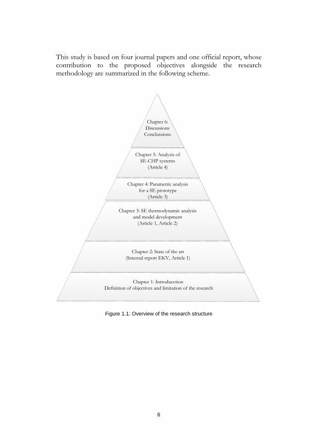
This study is based on four journal papers and one official report, whose contribution to the proposed objectives alongside the research methodology are summarized in the following scheme.

Chapter 1: Introducction Definition of objectives and limitation of the research

Chapter 6: Discussions

Conclussions

Chapter 2: State of the art(Internal report EKV, Article 1)

Chapter 3: SE thermodynamic analysis and model development

(Article 1, Article 2)

Chapter 4: Parametric analysis for a SE prototype

(Article 3)

Chapter 5: Analysis of SE-CHP systems

(Article 4)

Figure 1.1: Overview of the research structure

6

2 The Stir l ing engine technology: Overview and CHP applications

The Stirling engine is a thermal machine that operates in a closed thermodynamic cycle, named Stirling cycle. This cycle includes a regenerative heat transfer process between a cyclic compression-expansion of the working fluid at different temperature levels [24]. This definition includes power systems, where there is a net conversion of heat to work; and also work-consuming systems such as refrigerators and heat pumps.

Robert Stirling patented the first Stirling engine in 1816 [25]. This patent included the description of two innovative concepts: The closed cycle air engine and the economiser heat exchanger (regenerator). The invention was extraordinary for those times, considering that the understanding of the thermodynamic concepts of heat and work were very limited, and only by 1824 Carnot published the first analysis for heat engines [26]. The patent was the basis for the construction of the first Stirling engine, which was built by James and Robert Stirling. This engine, aimed to provide 2 HP of power, but only succeeded to drive a water pump in a quarry, until the air vessels became overheated and crushed down [27].

After the first patent, the engine has had a slow evolution. The first improvements were implemented by the Stirling brothers[28]. These included the development of a cooling system, improvements on the sealing for operation at higher pressures, and the use of regenerator materials in forms of wires-gauze that improved the heat transfer rate [29]. The improvements were applied for the construction of different engines. Among these one of the most successful engines was a 45 HP engine that was installed to drive all the machines of the Dundee Foundry in 1843[30]. This engine worked around 4 years, with an efficiency that reached around 18%, much better that the steam engines available at that time. However, the engine had many shut downs due to the air vessels problems [30]. For this reason it was later replaced by the steam engine, which was less efficient but with a more reliable operation.

The Dundee engine reflected the situation of the Stirling engine during the 19th century, a very promising engine but with unpredictable stability and thus not desirable for industrial purposes that prioritized reliability

7

over efficiency. These constructional problems limited the size of Stirling engines and relegated his development to small units used for small purposes such as driving fans and similar light duties[31]. This limitation was enhanced with the subsequent development of internal combustion engines, that presented more benefits in terms of efficiency and power outputs over the Stirling engines [32].

The second revolution for the Stirling engine began around 1937, when the Phillips Research Laboratory started the development of a small Stirling unit capable of generate 16 W of electricity, suitable for power portable radios sets[33]. The performance of this engine overpassed the expectative and thus boosted the research on the engine. Therefore, from 1937 until 1953, the Stirling engine was brought to a high state of technological development by the Phillips Research Laboratory[34]. During this period different engine prototypes were developed. These covered small units such as the 16 W single displacer engine, medium size units 500 W engines, double acting four cylinder engines 6 kW, and also some large units such as the 90 HP engine built in 1948 [33]. These engines portrayed improvements attributed to the application of heat resistant materials, better lubrication of the pistons, improvement of the seals, better regenerator materials, and innovative cranck mechanisms. In addition, the support of the advances on heat transfer, thermodynamics, and fluid flow theories, allowed obtaining increased power to weight ratios by a factor of 50 and power per unit swept volume by about 125[33]. The successful results of the Phillips engines were the base for further research in cooperation with prestigious companies and research institutes, such as General Motors, NASA, U.S. Navy, U.S. Army, Ford, United Stirling, and Stirling thermal motors among others[35]. However, despite of the high technical quality of the engines, the problems with the commercialization, costs and the difficulty to compete in a market dominated by the ICE limited again the engine success. It is in recent years that the increasing prices of fossil fuels, and the growing environmental problems, have sparkled again the fuel flexibility and low emissions advantages of the Stirling engine[9]. However, the perspective is different and the interest in the engine has turned towards its potential as main component of solar concentrator systems and the small scale heat and power plants[14]. Some examples correspond to the prototype tests reported by Sato[36], Nishiyama[37], Biederman[38], Pålsson[39], Zeiler[40], Thomas,[11] and Reddy[41].However, the Stirling engine technology is still not fully developed and furthermore its integration into the CHP systems presents many challenges. For these reasons, this research is guided towards the analysis of the CHP-SE technology and its potential for electricity services.

8

2 . 1 T e c h n o l o g y o v e r v i e w

The Stirling engine is defined by Walker [42] as: “A device which operates on a closed regenerative thermodynamic cycle, with cyclic compression and expansion of the working fluid at different temperature levels and where the flow is controlled by volume changes, so that there is a net conversion of heat to work or vice versa”. The thermodynamic cycle is known as a Stirling cycle, and although the real engine behaviour differs greatly from this ideal cycle, this is still useful to describe the main principles that guide the engine operation.

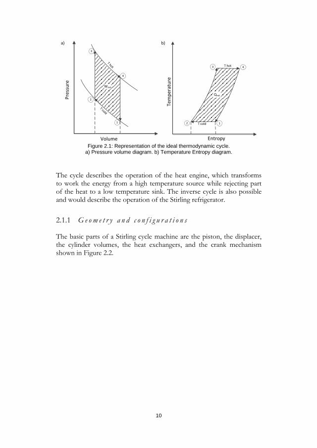
The ideal cycle consists of the processes represented in the pressure- volume and temperature-entropy diagrams shown in Figure 2.1.a and Figure 2.1.b. respectively:

- Isothermal compression (1-2): The working gas is compressed at a constant temperature (Tcold). The temperature is kept constant assuming that the heat increment is immediately transferred to an external heat sink. During this process the entropy reduces due to the heat transferred to the sink as seen in the entropy diagram - Isochoric heat addition (2-3): The working gas is heated until the higher temperature (Thot), while the total volume is kept constant. This process occurs inside the engine regenerator with a corresponding entropy increment. - Isothermal expansion (3-4): The working gas expands at a constant temperature (Thot). The heat needed to maintain the constant temperature is absorbed from an external heat source at an infinite heat transfer rate. The entropy increases due to heat input. - Isochoric cooling (4-1): The working gas is cooled to the lower temperature level (Tcold), while the total volume is kept constant. This process occurs also inside the regenerator, but with an entropy reduction.

9

Wnet

1

2

3

4

Pres

sure

Volume

T hot

T cold

12

3 4

Entropy

T hot

T cold

Tem

pera

ture

QnetQnet

a) b)

Figure 2.1: Representation of the ideal thermodynamic cycle.

a) Pressure volume diagram. b) Temperature Entropy diagram.

The cycle describes the operation of the heat engine, which transforms to work the energy from a high temperature source while rejecting part of the heat to a low temperature sink. The inverse cycle is also possible and would describe the operation of the Stirling refrigerator.

G e o m e t r y a n d c o n f i g u r a t i o n s 2.1.1

The basic parts of a Stirling cycle machine are the piston, the displacer, the cylinder volumes, the heat exchangers, and the crank mechanism shown in Figure 2.2.

10

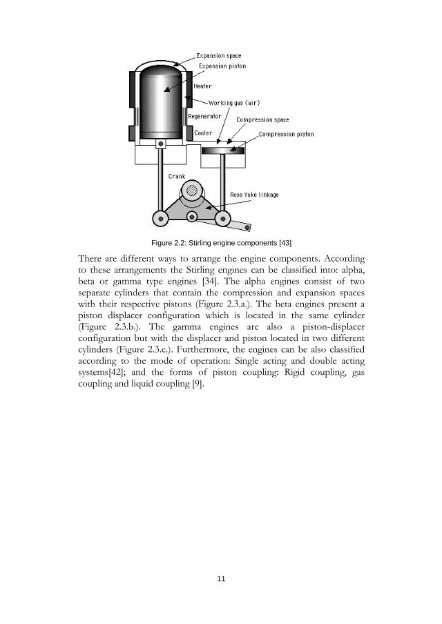
Figure 2.2: Stirling engine components [43]

There are different ways to arrange the engine components. According to these arrangements the Stirling engines can be classified into: alpha, beta or gamma type engines [34]. The alpha engines consist of two separate cylinders that contain the compression and expansion spaces with their respective pistons (Figure 2.3.a.). The beta engines present a piston displacer configuration which is located in the same cylinder (Figure 2.3.b.). The gamma engines are also a piston-displacer configuration but with the displacer and piston located in two different cylinders (Figure 2.3.c.). Furthermore, the engines can be also classified according to the mode of operation: Single acting and double acting systems[42]; and the forms of piston coupling: Rigid coupling, gas coupling and liquid coupling [9].

11

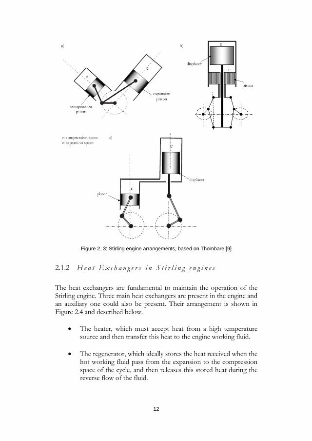
Figure 2. 3: Stirling engine arrangements, based on Thombare [9]

H e a t E x c h a n g e r s i n S t i r l i n g e n g i n e s 2.1.2

The heat exchangers are fundamental to maintain the operation of the Stirling engine. Three main heat exchangers are present in the engine and an auxiliary one could also be present. Their arrangement is shown in Figure 2.4 and described below.

• The heater, which must accept heat from a high temperature source and then transfer this heat to the engine working fluid.

• The regenerator, which ideally stores the heat received when the hot working fluid pass from the expansion to the compression space of the cycle, and then releases this stored heat during the reverse flow of the fluid.

12

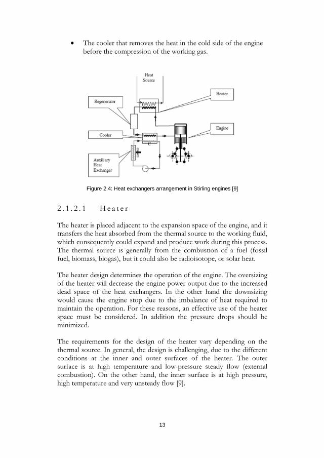
• The cooler that removes the heat in the cold side of the engine before the compression of the working gas.

Figure 2.4: Heat exchangers arrangement in Stirling engines [9]

2 . 1 . 2 . 1 H e a t e r

The heater is placed adjacent to the expansion space of the engine, and it transfers the heat absorbed from the thermal source to the working fluid, which consequently could expand and produce work during this process. The thermal source is generally from the combustion of a fuel (fossil fuel, biomass, biogas), but it could also be radioisotope, or solar heat.

The heater design determines the operation of the engine. The oversizing of the heater will decrease the engine power output due to the increased dead space of the heat exchangers. In the other hand the downsizing would cause the engine stop due to the imbalance of heat required to maintain the operation. For these reasons, an effective use of the heater space must be considered. In addition the pressure drops should be minimized.

The requirements for the design of the heater vary depending on the thermal source. In general, the design is challenging, due to the different conditions at the inner and outer surfaces of the heater. The outer surface is at high temperature and low-pressure steady flow (external combustion). On the other hand, the inner surface is at high pressure, high temperature and very unsteady flow [9].

13

The design of the heater is guided by the evaluation of appropriate heat transfer coefficients for the heating process. In general the following heat transfer mechanism represents this process.

a) Convective and irradiative heat transfer from the external heat source to the external area of the tubes at the heater.

b) Conductive heat transfer from the outer to the inner surface of the heat exchanger.

c) Convective heat transfer from the inner surface to the working fluid.

For the heat transfer between the heat source and the external wall of the heater, correlations based on radiative and convective mechanisms are found in the literature[44][10]. On the other hand, there are few proper correlations for the unsteady conditions of the working fluid inside the heater. Early approaches assumed mean values and steady heat transfer correlations[45], but recently some correlations for steady state cyclic conditions were also reported [46][47].

Another aspect to consider for the heater design is the fact that the power output of the engine is greater at higher temperatures. For this reason materials resistant to high temperature loads such as advanced super alloys, refractory metal alloys, and ceramics are necessary to increase the resistance of the heater [48]. For example advanced super alloys may permit operations at 750 to 850 °C, while refractory metal alloys and ceramics could achieve up to about 1200 °C [49]. The fouling effect must be also considered for the heater design. According to Palsson and Carlsten [39], in the case of solid bio fuels, which give high amount of ash residue when burned, the ash starts to melt and gets sticky above a certain temperature. This leads to build-up of ash at the heater, and for this reason it is necessary to keep the temperature of the combustion chamber below to the melting point of the ash. Otherwise, the fouling will highly reduce the efficiency of the Stirling engine [50].

The mentioned design considerations for the heater brought the development of different design alternatives that have evolved from the simplest first heat exchanger[51]. These alternatives can be classified into: annular, tubular and finned heat exchangers[52]. Annular heat exchangers consist of concentric tubes containing the fluid between them. Tubular designs contain one fluid within small diameter tubes surrounded by the other heat exchanging fluid. Finned designs increase the heat transfer area thanks to finned structures. The combination of annular finned and tubular finned designs have also been developed[53]. Figure 2.5 shows the heater head of the described tubular and annular

14

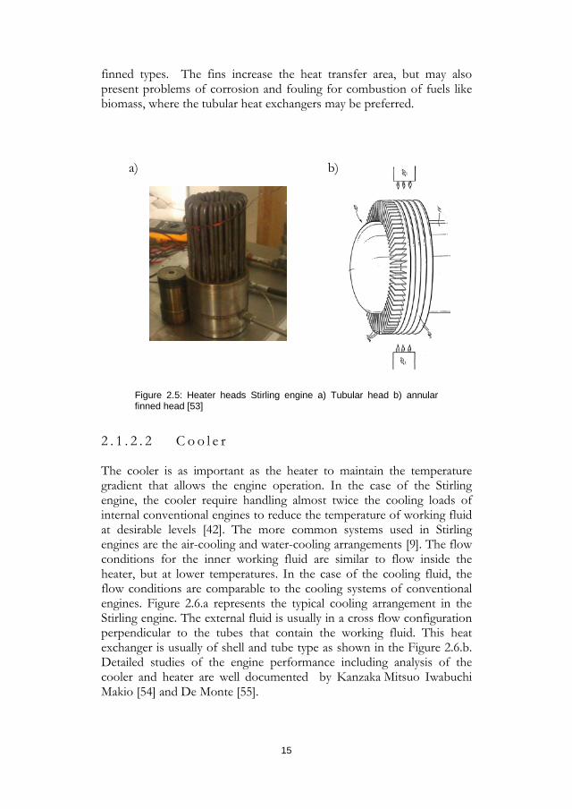
finned types. The fins increase the heat transfer area, but may also present problems of corrosion and fouling for combustion of fuels like biomass, where the tubular heat exchangers may be preferred.

a) b)

Figure 2.5: Heater heads Stirling engine a) Tubular head b) annular finned head [53]

2 . 1 . 2 . 2 C o o l e r

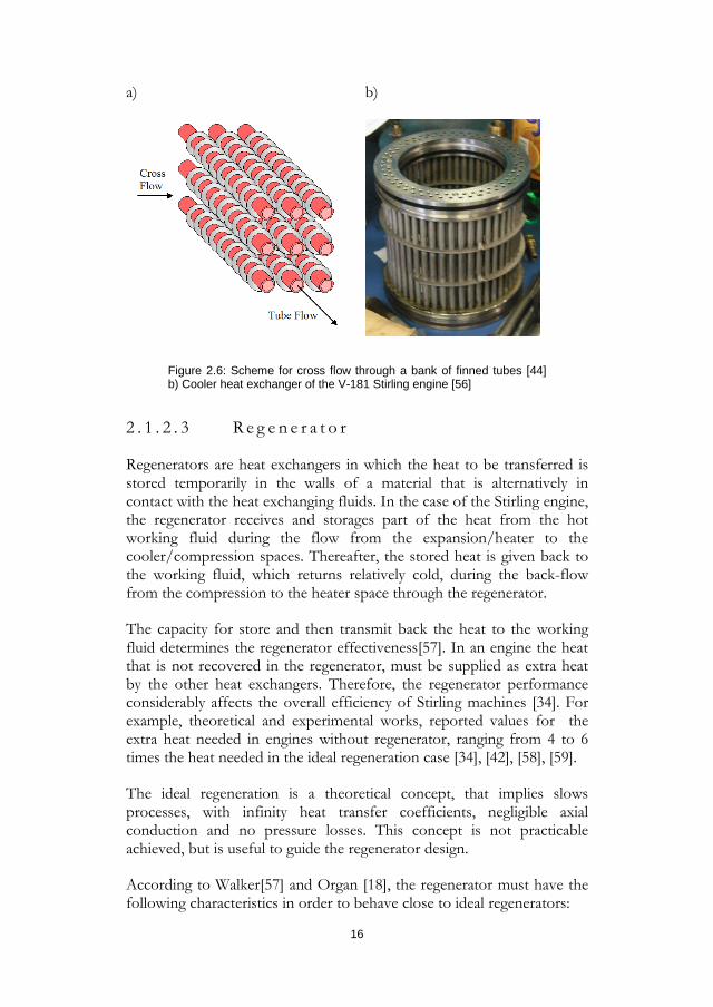
The cooler is as important as the heater to maintain the temperature gradient that allows the engine operation. In the case of the Stirling engine, the cooler require handling almost twice the cooling loads of internal conventional engines to reduce the temperature of working fluid at desirable levels [42]. The more common systems used in Stirling engines are the air-cooling and water-cooling arrangements [9]. The flow conditions for the inner working fluid are similar to flow inside the heater, but at lower temperatures. In the case of the cooling fluid, the flow conditions are comparable to the cooling systems of conventional engines. Figure 2.6.a represents the typical cooling arrangement in the Stirling engine. The external fluid is usually in a cross flow configuration perpendicular to the tubes that contain the working fluid. This heat exchanger is usually of shell and tube type as shown in the Figure 2.6.b. Detailed studies of the engine performance including analysis of the cooler and heater are well documented by Kanzaka Mitsuo Iwabuchi Makio [54] and De Monte [55].

15

http://adsabs.harvard.edu/cgi-bin/author_form?author=Kanzaka,+M&fullauthor=Kanzaka,%20Mitsuo&charset=UTF-8&db_key=PHY

http://adsabs.harvard.edu/cgi-bin/author_form?author=Iwabuchi,+M&fullauthor=Iwabuchi,%20Makio&charset=UTF-8&db_key=PHY

http://adsabs.harvard.edu/cgi-bin/author_form?author=Iwabuchi,+M&fullauthor=Iwabuchi,%20Makio&charset=UTF-8&db_key=PHY

a)

b)

Figure 2.6: Scheme for cross flow through a bank of finned tubes [44] b) Cooler heat exchanger of the V-181 Stirling engine [56]

2 . 1 . 2 . 3 R e g e n e r a t o r

Regenerators are heat exchangers in which the heat to be transferred is stored temporarily in the walls of a material that is alternatively in contact with the heat exchanging fluids. In the case of the Stirling engine, the regenerator receives and storages part of the heat from the hot working fluid during the flow from the expansion/heater to the cooler/compression spaces. Thereafter, the stored heat is given back to the working fluid, which returns relatively cold, during the back-flow from the compression to the heater space through the regenerator.

The capacity for store and then transmit back the heat to the working fluid determines the regenerator effectiveness[57]. In an engine the heat that is not recovered in the regenerator, must be supplied as extra heat by the other heat exchangers. Therefore, the regenerator performance considerably affects the overall efficiency of Stirling machines [34]. For example, theoretical and experimental works, reported values for the extra heat needed in engines without regenerator, ranging from 4 to 6 times the heat needed in the ideal regeneration case [34], [42], [58], [59].

The ideal regeneration is a theoretical concept, that implies slows processes, with infinity heat transfer coefficients, negligible axial conduction and no pressure losses. This concept is not practicable achieved, but is useful to guide the regenerator design.

According to Walker[57] and Organ [18], the regenerator must have the following characteristics in order to behave close to ideal regenerators:

16

• Maximum heat capacity, which implies large solid materials • Minimum flow losses, which implies highly porous matrixes. • Minimum dead space, then a small dense matrix is required • Maximum heat transfer, then large finely divided matrix is required • Minimum contamination, then matrix with no obstruction is

required • Homogenous matrix and good sealing at the periphery to avoid

preferential flows paths

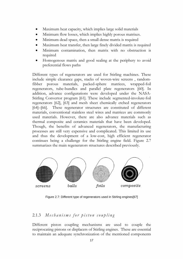
Different types of regenerators are used for Stirling machines. These include simple clearance gaps, stacks of woven-wire screens , random-fibber porous materials, packed-sphere matrices, wrapped-foil regenerators, tube-bundles and parallel plate regenerators [60]. In addition, advance configurations were developed under the NASA- Stirling Convertor program [61]. These include segmented-involute-foil regenerators [62], [63] and mesh sheet chemically etched regenerators [64]–[66]. These regenerator structures are constituted of different materials, conventional stainless steel wires and matrices are commonly used materials. However, there are also advance materials such as thermal composite and ceramics materials that have been developed. Though, the benefits of advanced regenerators, the manufacturing processes are still very expensive and complicated. This limited its use and thus the development of a low-cost, high efficient regenerator continues being a challenge for the Stirling engine field. Figure 2.7 summarizes the main regenerators structures described previously.

Figure 2.7: Different type of regenerators used in Stirling engines[67]

M e c h a n i s m s f o r p i s t o n c o u p l i n g 2.1.3

Different piston coupling mechanisms are used to couple the reciprocating pistons or displacers of Stirling engines. These are essential to maintain an adequate synchronization of the mentioned components

17

and thus have an important influence on the engine operation. Adequate mechanisms will reduce the axial movements of piston rods, minimize lateral forces and vibrations, and provide a complete balance of all the inertial forces [34]. The mechanism is directly connected to the buffer space that contains the working gas of the engine cylinders and therefore it has an important role for the adequate sealing of the engine. The following section describes the most common mechanisms used in Stirling engines.

• Simple slider crank drive. The slider crank has been successfully used for many years on internal combustion engines due to its reliability and easy manufacture. Nowadays is used for double acting Stirling engines. However this mechanism has the disadvantage of being very difficult to balance [9]. (Fig. 2.8.a)

• Rhombic Drive. This is one of the most well developed and frequently used in single cylinder Stirling engines. It was developed by Philips in 1950 and since the beginning showed the necessary dynamic balance for piston-displacer engines. The main disadvantage is the large number of moving parts that must be well synchronized and thus complicates its manufacture (Fig. 2.8.b). [34]

• Swash plate. This system is dynamically balanced with the use of a swash plate (Fig.2.8 c). The advantage is that the use of the fixed plate permit a better sealing system, and therefore it is useful for applications with large numbers of fast cycle requirements [9]. The system permits also to control the power output by changing the stroke of the engine with the variation of the plate’s angle [34]. The company STM Inc., now acquired by Stirling Power [68], developed a four piston prototype based on this mechanism.

• Ross joker. This mechanism was patented by Andy Ross [69], who developed a Stirling engine using the linkage illustrated in Figure 2.8.d. The operation of this system is similar to the two cylinder designs. The advantage is that the mechanism is more compact, and also reduces side loads on the pistons and connecting rods.

• Ringbom mechanism. This arrangement is similar to the free piston configuration. The piston link with the crank shaft is mechanic but the displacer is driven by the gas forces, which are powered by the difference in pressure between the internal gas and atmospheric pressure (Fig.2.8.e). The usage of this is more common in small prototypes of Stirling engines around 30W of electrical output[9].

18

• Free piston engine. This arrangement does not use a mechanical linkage for the piston and displacer. For this reason the piston is free mechanically, but with a gas spring that provides a similar effect of the mechanical link. These permits a better sealing because no piston rod has to cross the crankcase [70]. The configuration is shown in Figure 2.8.f. The advantages of this system are the reduction of maintenance, and the possibility to develop more compact engines. This potential encouraged a program for the development of advanced radioisotope Stirling convertors that aimed to implement these engines for space exploration [71]. However, the costs and the improvement on the sealing are still challenges to be improved [72].

19

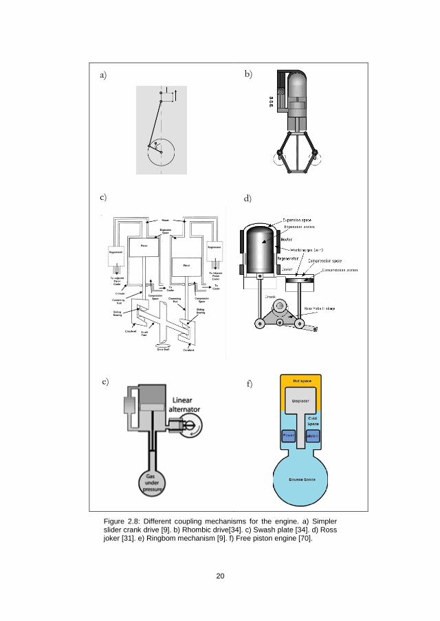
Figure 2.8: Different coupling mechanisms for the engine. a) Simpler slider crank drive [9]. b) Rhombic drive[34]. c) Swash plate [34]. d) Ross joker [31]. e) Ringbom mechanism [9]. f) Free piston engine [70].

a) b)

c) d)

e) f)

20

2 . 2 S t i r l i n g e n g i n e c o m b i n e d h e a t a n d p o w e r s y s t e m s

The Stirling engine (SE) presents potential for applications like combined heat and power (CHP), and combined cool heat and power (CCHP) plants. The literature reports also studies for the integration of SE in waste incineration processes [10], gas reforming processes [73], and fuel cells systems [74]. The implementation of these systems should previously evaluate parameters related to thermal and electrical efficiency, performance, maintenance, emissions and costs of these technologies. This section shows the results from these reported experiences and aims to describe its degree of development.

S y s t e m e f f i c i e n c y 2.2.1

Micro and small scale CHP-SE systems are fuelled by natural gas, solar radiation, and biomass (wood or agricultural residues). For these reason, the electrical and thermal efficiency varies depending of the fuel used for the heat generation process. For example, table 2.1.reports variations from 10% to 24 % for the electrical efficiency and 55% to 85% for thermal efficiency with different fuels.

Some experiences for SE systems fuelled by natural gas are reported in the work of Bernd [11]. This work evaluates the performance of two micro CHP units: The SOLO 161 engine built in that time by SOLO Company and the micro CHP SM5A developed by Stirling Denmark. The performance of both engines presented good efficiencies with values in the order of 20% electrical and 65% thermal efficiencies. These results were good exhibitions of the engine potential. Klemes [75], also presented reports for natural gas fuelled systems: The Solo 161 SE CHP in Germany and the WhisperGen SE system in France and Netherlands. In these cases the results reflected a good performance for the SOLO system but the performance of the Whispergen system was much lower than expected.

In the cases of biomass fuels for SE-CHP, the electrical efficiencies reported are very low. For example, Bierderman[38] reported results of a 35 kW plant that operated during 5000 hours with electrical efficiencies around 10%. Obara[76], also present results for electrical efficiencies around 12 % for a SE prototype built for cold region houses and fuelled with biomass. Table 2.1 summarizes the mentioned experiences. These results reflect the need for improvements on biomass fuelled systems. These improvements may focus the attention on minimizing the fouling,

21

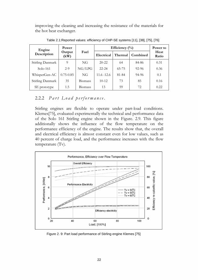
improving the cleaning and increasing the resistance of the materials for the hot heat exchanger.

Table 2.1:Reported values: efficiency of CHP-SE systems [11], [38], [75], [76]

Engine Description

Power Output (kW)

Fuel Efficiency (%) Power to

Heat Ratio Electrical Thermal Combined

Stirling Danmark 9 NG 20-22 64 84-86 0.31

Solo-161 2-9 NG/LPG 22-24 65-75 92-96 0.36

WhisperGen-AC 0.75-0.85 NG 11.6 -12.6 81-84 94-96 0.1

Stirling Danmark 35 Biomass 10-12 73 85 0.16

SE prototype 1.5 Biomass 13 59 72 0.22

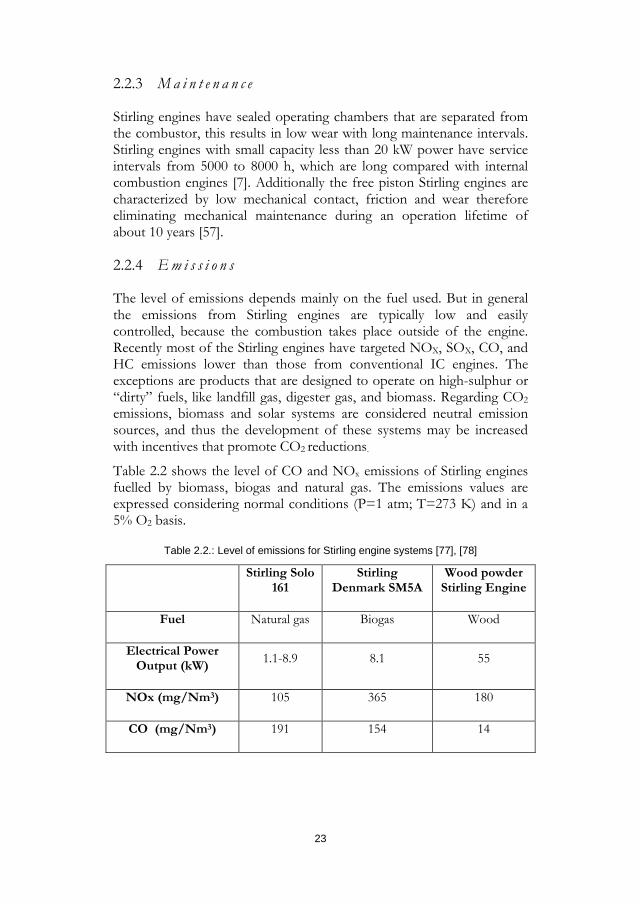
P a r t L o a d p e r f o r m a n c e . 2.2.2 Stirling engines are flexible to operate under part-load conditions. Klemes[75], evaluated experimentally the technical and performance data of the Solo 161 Stirling engine shown in the Figure. 2.9. This figure additionally shows the influence of the flow temperature on the performance efficiency of the engine. The results show that, the overall and electrical efficiency is almost constant even for low values, such as 40 percent of charge load, and the performance increases with the flow temperature (Tv).

Figure 2. 9: Part load performance of Stirling engine Klemes [75]

22

M a i n t e n a n c e 2.2.3

Stirling engines have sealed operating chambers that are separated from the combustor, this results in low wear with long maintenance intervals. Stirling engines with small capacity less than 20 kW power have service intervals from 5000 to 8000 h, which are long compared with internal combustion engines [7]. Additionally the free piston Stirling engines are characterized by low mechanical contact, friction and wear therefore eliminating mechanical maintenance during an operation lifetime of about 10 years [57].

E m i s s i o n s 2.2.4

The level of emissions depends mainly on the fuel used. But in general the emissions from Stirling engines are typically low and easily controlled, because the combustion takes place outside of the engine. Recently most of the Stirling engines have targeted NOX, SOX, CO, and HC emissions lower than those from conventional IC engines. The exceptions are products that are designed to operate on high-sulphur or “dirty” fuels, like landfill gas, digester gas, and biomass. Regarding CO2 emissions, biomass and solar systems are considered neutral emission sources, and thus the development of these systems may be increased with incentives that promote CO2 reductions.

Table 2.2 shows the level of CO and NOx emissions of Stirling engines fuelled by biomass, biogas and natural gas. The emissions values are expressed considering normal conditions (P=1 atm; T=273 K) and in a 5% O2 basis.

Table 2.2.: Level of emissions for Stirling engine systems [77], [78]

Stirling Solo 161

Stirling Denmark SM5A

Wood powder Stirling Engine

Fuel Natural gas Biogas Wood

Electrical Power Output (kW) 1.1-8.9 8.1 55

NOx (mg/Nm3) 105 365 180

CO (mg/Nm3) 191 154 14

23

C o s t a n d C o m m e r c i a l a v a i l a b i l i t y 2.2.5

This is one of the weak points on the Stirling engine technology. Most of the engines are in a development stage and only prototypes are commercially available. In general natural gas fuelled Stirling engines are more developed. For example, companies like Whisper gen[79] and Stirling Solo[80] have developed different engine prototypes. Additionally companies such as Stirling Sun Power [81], Infinia(Qnergy) [82] , Cleanergy [83] have solar driven engines commercially available. The development of biomass fuelled engines is delayed with only some tested technologies like the Stirling Denmark 35kW wood-fuelled [84], and Cleanergy biomass CHP plant [83]. Due to the prototype stage, the prices for the engines differ largely among companies. Few studies compared the price modelling for the SE prototypes, and commercial prices around 1125-3000 $/kW were reported [85].

24

3 Thermodynamic modeling and analysis of Stir l ing engines

The development of Stirling engines requires the understanding of the processes that governs their operation. The first attempt to describe this process was trough the ideal Stirling thermodynamic cycle. But, this cycle does not reflect the real interactions presented in the engine. This has promoted the emergence of various analysis techniques with different modelling approaches. The majority of these techniques are mainly focused on the description of the internal gas circuit of the engine, and few studies considered other interactions. For this reason the present study proposed the development of a model that could integrate the heat transfer phenomena, the thermodynamics and the mechanical efficiency to describe the operation of Stirling engine systems. Furthermore, the model also included the external heat transfer interactions with the hot and cold energy sources. The details for the development of the proposed model are described in article I. This chapter summarizes this study.

3 . 1 R e v i e w o f d i f f e r e n t a n a l y s i s t e c h n i q u e s

The different techniques for the analysis of Stirling engines can be classified with different criterions. The criterion adopted in this section is based on the review of Dyson et al [19]. According to this criteria, the techniques could be categorized into zero order, approximate (first order), decoupled (second order), nodal analysis (third order), and the recently multidimensional analysis (fourth order). This is shown in Figure 3.1.

25

Stirling engine analysis techniques

0th order 1st order 2nd order 3rd order

Empirical correlations

(Beale equation)

Isothermic models

Schmidth analysis

Decoupled approach

Nodal models

4th order

CFD models

Method of characteristics

Adiabatic models

Modified adiabatic models

Coupled approach

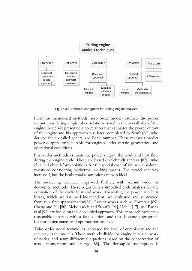
Figure 3.1: Different categories for Stirling engine analysis

From the mentioned methods, zero order models estimate the power output considering empirical correlations based in the overall size of the engine. Beale[42] presented a correlation that estimates the power output of the engine and his approach was later completed by Senft [86], who derived the so called generalized Beale number. These methods predict power outputs, only suitable for engines under certain geometrical and operational conditions.

First order methods estimate the power output, the work and heat flow during the engine cycle. These are based on Schmidt analysis [87], who obtained closed-form solutions for the special case of sinusoidal volume variations considering isothermal working spaces. The model accuracy increased, but the isothermal assumptions remain ideal.

The modelling accuracy improved further, with second order or decoupled methods. These begin with a simplified cycle analysis for the estimation of the cyclic heat and work. Thereafter, the power and heat losses, which are assumed independent, are evaluated and subtracted from this first approximation[88]. Recent works such as Formosa [89], Cheng and Yu [90], Mehdizadeh and Stouffs [91], Urielli [17], and Parlak et al [92] are based on this decoupled approach. This approach presents a reasonable accuracy with a fast solution, and thus became appropriate for fast design stages and optimization studies.

Third order nodal techniques increased the level of complexity and the accuracy in the models. These methods divide the engine into a network of nodes, and setup differential equations based on the conservation of mass, momentum and energy [88]. The decoupled assumption is

26

replaced by including the evaluation of the different energy losses within the governing equations. Some of the analyses at this level were developed by Finkelstein [93], Urielli [94], Schock [95], Gedeon [96] and Tew et al [97]. In addition Organ [98] and Larson [99], simplified the model solution using the method of characteristics for the case of unsteady one-dimensional flow. These methods present a detailed description of the engine performance, considering the heat and work flows and the thermal and mechanical losses. However, the computational time is largely increased and thus became not suitable for optimization studies.

Modern fourth order methods or multidimensional analysis have been recently developed. These use computer fluid dynamic (CFD) simulation codes. These multi-dimensional models provide detailed information regarding the flow pattern, temperature, and pressure distributions inside the engine. The main limitation of these models is that requires much more computation efforts which are expensive and restricted to detailed engine design. This approach was used by Mahkamov [100], Ibrahim [101] and Wilson et al [71].

3 . 2 P r o p o s e d s e c o n d o r d e r t h e r m o d y n a m i c m o d e l

The validity of the techniques described in the previous section depends on the type of study and the data available. For example, first order methods are useful to guide the optimization of already built prototypes that have been widely studied experimentally. On the other extreme, multidimensional methods are more suitable for studies that could guide novel designs in a stage previous to the prototype manufacture.

The present study aims for an overall analysis of SE-CHP systems. Hence the engine model must be flexible and should allow the analysis of the engine integration into overall systems. This integrated approach was considered by few simulation studies [102]–[106]. However, these studies considered models closer to the “black box” zeroth order types, and consequently does not reflect the thermodynamics of the engine. For these reasons, a simulation tool for the analysis of SE systems was developed. This tool presents a modular structure that permits the interconnection of the different components of the engine and the integration within overall systems.

The basis for the simulation tool is a numerical model, which considers the thermodynamics, heat transfer, fluid dynamics and mechanical efficiency of the engine. In addition, permits studies for design optimization and integration within overall CHP systems.

27

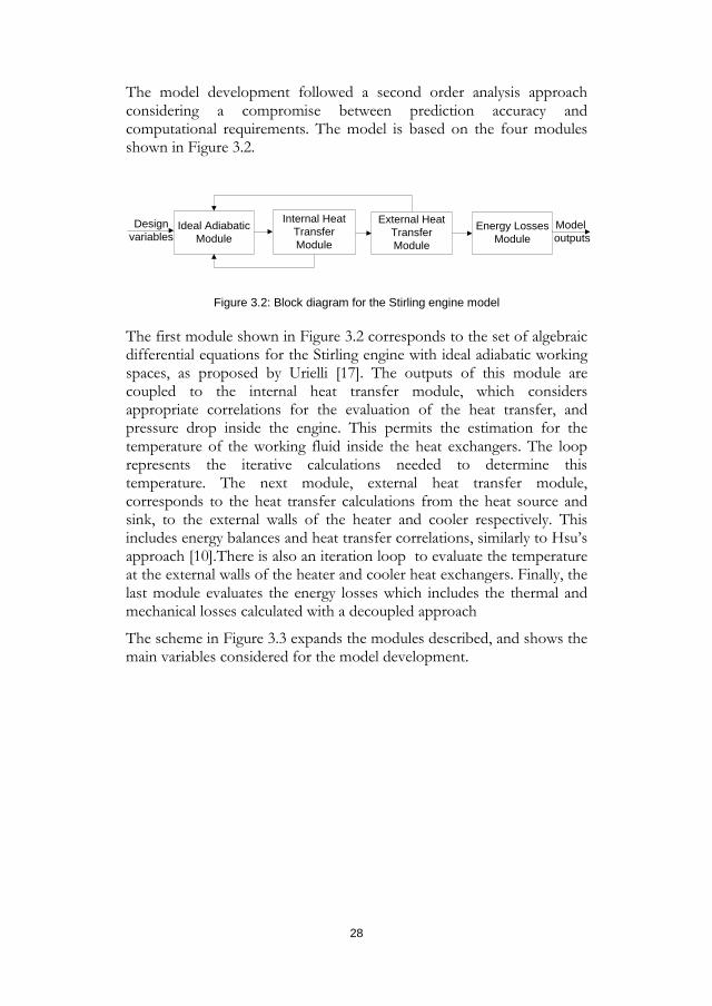
The model development followed a second order analysis approach considering a compromise between prediction accuracy and computational requirements. The model is based on the four modules shown in Figure 3.2.

Ideal Adiabatic Module

Internal Heat Transfer Module

External Heat Transfer Module

Energy Losses Module

Design variables

Model outputs

Figure 3.2: Block diagram for the Stirling engine model

The first module shown in Figure 3.2 corresponds to the set of algebraic differential equations for the Stirling engine with ideal adiabatic working spaces, as proposed by Urielli [17]. The outputs of this module are coupled to the internal heat transfer module, which considers appropriate correlations for the evaluation of the heat transfer, and pressure drop inside the engine. This permits the estimation for the temperature of the working fluid inside the heat exchangers. The loop represents the iterative calculations needed to determine this temperature. The next module, external heat transfer module, corresponds to the heat transfer calculations from the heat source and sink, to the external walls of the heater and cooler respectively. This includes energy balances and heat transfer correlations, similarly to Hsu’s approach [10].There is also an iteration loop to evaluate the temperature at the external walls of the heater and cooler heat exchangers. Finally, the last module evaluates the energy losses which includes the thermal and mechanical losses calculated with a decoupled approach

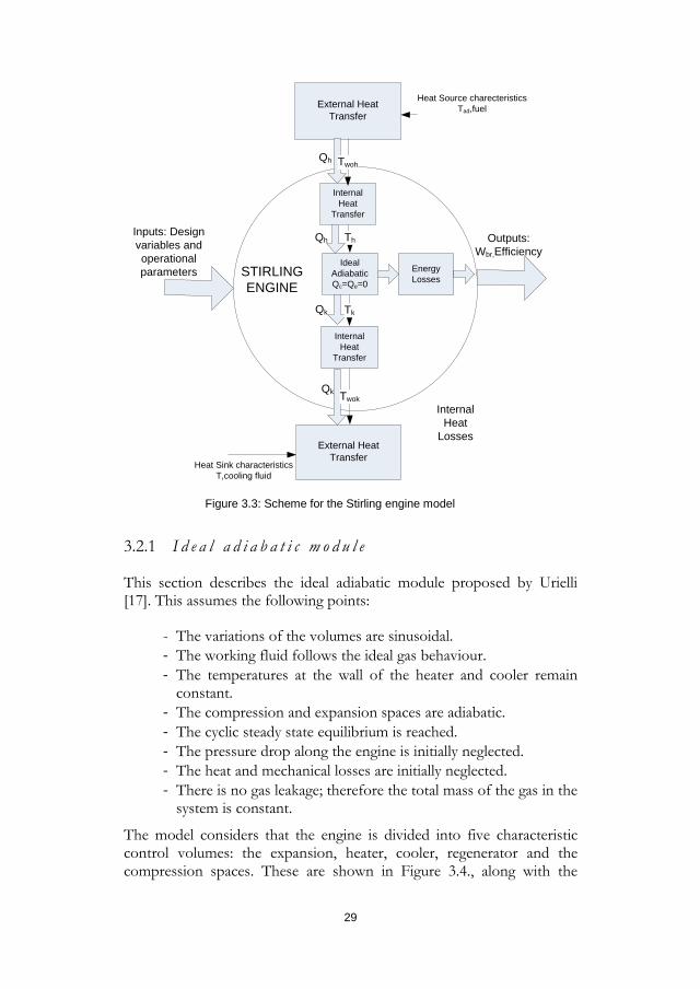
The scheme in Figure 3.3 expands the modules described, and shows the main variables considered for the model development.

28

Internal Heat

Losses

External Heat Transfer

Internal Heat

Transfer

Heat Source charecteristicsTad,fuel

Ideal Adiabatic Qc=Qe=0

Th

Internal Heat

Transfer

External Heat Transfer

Heat Sink characteristicsT,cooling fluid

Outputs: Wbr,Efficiency

Twoh

Tk

Twok

STIRLING ENGINE

Qh

Qh

Qk

Qk

Inputs: Design variables and operational parameters Energy

Losses

Figure 3.3: Scheme for the Stirling engine model

I d e a l a d i a b a t i c m o d u l e 3.2.1

This section describes the ideal adiabatic module proposed by Urielli [17]. This assumes the following points:

- The variations of the volumes are sinusoidal. - The working fluid follows the ideal gas behaviour. - The temperatures at the wall of the heater and cooler remain

constant. - The compression and expansion spaces are adiabatic. - The cyclic steady state equilibrium is reached. - The pressure drop along the engine is initially neglected. - The heat and mechanical losses are initially neglected. - There is no gas leakage; therefore the total mass of the gas in the

system is constant.

The model considers that the engine is divided into five characteristic control volumes: the expansion, heater, cooler, regenerator and the compression spaces. These are shown in Figure 3.4., along with the

29

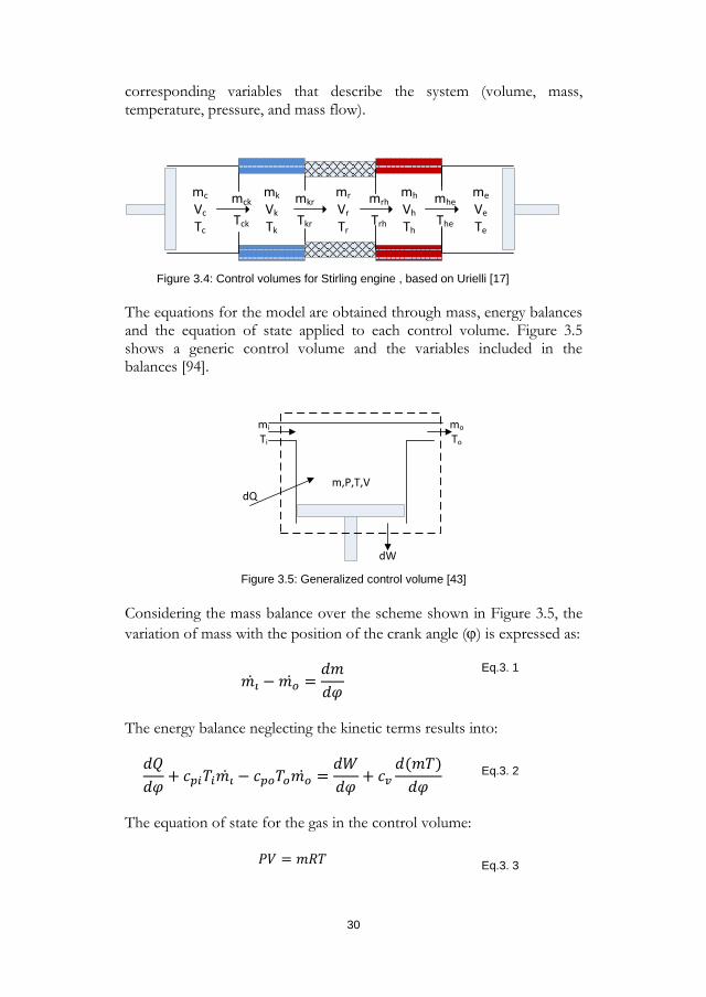
corresponding variables that describe the system (volume, mass, temperature, pressure, and mass flow).

mc

Vc

Tc

mk

Vk

Tk

mr

Vr

Tr

mh

Vh

Th

me

Ve

Te

mck

Tck

mkr

Tkr

mrh

Trh

mhe

The

Figure 3.4: Control volumes for Stirling engine , based on Urielli [17]

The equations for the model are obtained through mass, energy balances and the equation of state applied to each control volume. Figure 3.5 shows a generic control volume and the variables included in the balances [94].

m,P,T,V

mi

Ti

mo

To

dQ

dW

Figure 3.5: Generalized control volume [43] Considering the mass balance over the scheme shown in Figure 3.5, the variation of mass with the position of the crank angle (ϕ) is expressed as:

𝑚𝑚𝚤𝚤̇ − 𝑚𝑚𝑏𝑏̇ =𝑑𝑑𝑚𝑚𝑑𝑑𝜑𝜑

Eq.3. 1

The energy balance neglecting the kinetic terms results into: 𝑑𝑑𝑄𝑄𝑑𝑑𝜑𝜑

+ 𝑅𝑅𝑣𝑣𝑚𝑚𝑁𝑁𝑚𝑚𝑚𝑚𝚤𝚤̇ − 𝑅𝑅𝑣𝑣𝑏𝑏𝑁𝑁𝑏𝑏𝑚𝑚𝑏𝑏̇ =𝑑𝑑𝑊𝑊𝑑𝑑𝜑𝜑

+ 𝑅𝑅𝑣𝑣𝑑𝑑(𝑚𝑚𝑁𝑁)𝑑𝑑𝜑𝜑

Eq.3. 2

The equation of state for the gas in the control volume:

𝑃𝑃𝐶𝐶 = 𝑚𝑚𝑅𝑅𝑁𝑁 Eq.3. 3

30

Pressure and volume variations

The evaluation of the pressure along the engine is calculated considering the mass balance applied to the overall engine.

𝑚𝑚𝑐𝑐 + 𝑚𝑚𝑙𝑙 + 𝑚𝑚𝑟𝑟 + 𝑚𝑚ℎ + 𝑚𝑚𝑏𝑏 = 𝑀𝑀 Eq.3. 4

The mass balance is re-written in a form that allows the calculation of the pressure.

P=MR

VcTc

+ VkTk

+ VrTr

+ VhTh

+ VeTe

Eq.3. 5

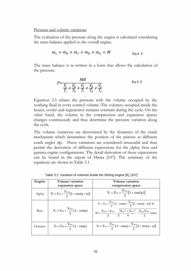
Equation 3.5 relates the pressure with the volume occupied by the working fluid in every control volume. The volumes occupied inside the heater, cooler and regenerator remains constant during the cycle. On the other hand, the volume in the compression and expansion spaces changes continuously and thus determine the pressure variation along the cycle.

The volume variations are determined by the dynamics of the crank mechanism which determines the position of the pistons at different crank angles (ϕ). These variations are considered sinusoidal and thus permit the derivation of different expressions for the alpha, beta and gamma engine configurations. The detail derivation of these expressions can be found in the report of Hirata [107]. The summary of the equations are shown in Table 3.1.

Table 3.1: Variation of volumes inside the Stirling engine [9], [107]

Engine Volume variation expansion space

Volume variation compression space

Alpha [ ]α)cos(12

VVV sweclee +ϕ++= [ ])cos(1

2VVV swc

clcc ϕ++=

Beta )cos(12

VVV sweclee ϕ−+=

[ ] Bswcswe

clcc V-α)cos(12

V)cos(12

VVV −ϕ−+ϕ−+=

cosα2VV

4VV

2VVV swc swe

2swc

2sweswcswe

B −+

−+

=

Gamma )cos(12

VVV sweclee ϕ−+= [ ]α)cos(1

2V)cos(1

2VVV swcswe

clcc −ϕ−+ϕ−+=

31

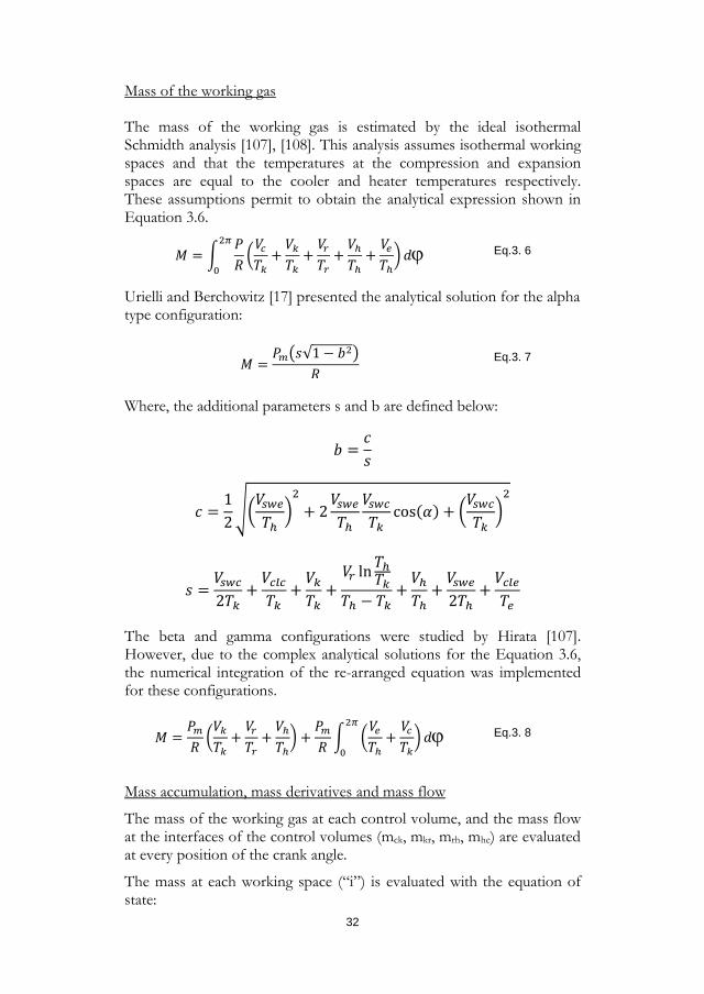
Mass of the working gas

The mass of the working gas is estimated by the ideal isothermal Schmidth analysis [107], [108]. This analysis assumes isothermal working spaces and that the temperatures at the compression and expansion spaces are equal to the cooler and heater temperatures respectively. These assumptions permit to obtain the analytical expression shown in Equation 3.6.

𝑀𝑀 = �𝑃𝑃𝑅𝑅

2𝜋𝜋

0�𝐶𝐶𝑐𝑐𝑁𝑁𝑙𝑙

+𝐶𝐶𝑙𝑙𝑁𝑁𝑙𝑙

+𝐶𝐶𝑟𝑟𝑁𝑁𝑟𝑟

+𝐶𝐶ℎ𝑁𝑁ℎ

+𝐶𝐶𝑏𝑏𝑁𝑁ℎ� 𝑑𝑑ϕ Eq.3. 6

Urielli and Berchowitz [17] presented the analytical solution for the alpha type configuration:

𝑀𝑀 =𝑃𝑃𝑚𝑚�𝑠𝑠√1 − 𝑏𝑏2�

𝑅𝑅 Eq.3. 7

Where, the additional parameters s and b are defined below:

𝑏𝑏 =𝑅𝑅𝑠𝑠

𝑅𝑅 =12��

𝐶𝐶𝑠𝑠𝑠𝑠𝑏𝑏𝑁𝑁ℎ

�2

+ 2𝐶𝐶𝑠𝑠𝑠𝑠𝑏𝑏𝑁𝑁ℎ

𝐶𝐶𝑠𝑠𝑠𝑠𝑐𝑐𝑁𝑁𝑙𝑙

cos(𝛼𝛼) + �𝐶𝐶𝑠𝑠𝑠𝑠𝑐𝑐𝑁𝑁𝑙𝑙

�2

𝑠𝑠 =𝐶𝐶𝑠𝑠𝑠𝑠𝑐𝑐2𝑁𝑁𝑙𝑙

+𝐶𝐶𝑐𝑐𝑏𝑏𝑐𝑐𝑁𝑁𝑙𝑙

+𝐶𝐶𝑙𝑙𝑁𝑁𝑙𝑙

+𝐶𝐶𝑟𝑟 ln𝑁𝑁ℎ𝑁𝑁𝑙𝑙𝑁𝑁ℎ − 𝑁𝑁𝑙𝑙

+𝐶𝐶ℎ𝑁𝑁ℎ

+𝐶𝐶𝑠𝑠𝑠𝑠𝑏𝑏2𝑁𝑁ℎ

+𝐶𝐶𝑐𝑐𝑏𝑏𝑏𝑏𝑁𝑁𝑏𝑏

The beta and gamma configurations were studied by Hirata [107]. However, due to the complex analytical solutions for the Equation 3.6, the numerical integration of the re-arranged equation was implemented for these configurations.

𝑀𝑀 =𝑃𝑃𝑚𝑚𝑅𝑅�𝐶𝐶𝑙𝑙𝑁𝑁𝑙𝑙

+𝐶𝐶𝑟𝑟𝑁𝑁𝑟𝑟

+𝐶𝐶ℎ𝑁𝑁ℎ� +

𝑃𝑃𝑚𝑚𝑅𝑅� �

𝐶𝐶𝑏𝑏𝑁𝑁ℎ

+𝐶𝐶𝑐𝑐𝑁𝑁𝑙𝑙�

2𝜋𝜋

0𝑑𝑑ϕ Eq.3. 8

Mass accumulation, mass derivatives and mass flow

The mass of the working gas at each control volume, and the mass flow at the interfaces of the control volumes (mck, mkr, mrh, mhe) are evaluated at every position of the crank angle.

The mass at each working space (“i”) is evaluated with the equation of state:

32

𝑚𝑚𝑚𝑚 =𝑃𝑃𝑅𝑅�𝐶𝐶𝑚𝑚𝑁𝑁𝑚𝑚�

𝑤𝑤: 𝑅𝑅, 𝑘𝑘, 𝑟𝑟, ℎ, 𝑅𝑅

Eq.3. 9

The derivatives of the mass “j” respect to the crank angle for each heat exchanger, which are assumed isothermal, are calculated from equation 3.10.

𝑑𝑑𝑚𝑚𝑗𝑗

𝑑𝑑ϕ =𝑚𝑚𝑗𝑗

𝑃𝑃�𝜕𝜕𝑃𝑃𝜕𝜕ϕ�

𝑗𝑗:𝑘𝑘, 𝑟𝑟, ℎ

Eq.3. 10

The derivatives for the compression and expansion spaces, which are not isothermal, are evaluated by the equations 3.11 and 3.12 below

𝑑𝑑𝑚𝑚𝑐𝑐

𝑑𝑑ϕ=𝑃𝑃 �𝜕𝜕𝐶𝐶𝑐𝑐𝜕𝜕ϕ� +

𝐶𝐶𝑐𝑐 �𝜕𝜕𝑃𝑃𝜕𝜕ϕ�𝛾𝛾

𝑅𝑅𝑁𝑁𝑐𝑐𝑙𝑙

Eq.3. 11

𝑑𝑑𝑚𝑚𝑏𝑏

𝑑𝑑ϕ=𝑃𝑃 �𝜕𝜕𝐶𝐶𝑏𝑏𝜕𝜕ϕ� +

𝐶𝐶𝑏𝑏 �𝜕𝜕𝑃𝑃𝜕𝜕ϕ�𝛾𝛾

𝑅𝑅𝑁𝑁ℎ𝑏𝑏

Eq.3. 12

The mass flows at the interfaces are evaluated with Eq. 3.1 applied to each control volume.

𝑚𝑚𝑐𝑐𝑙𝑙 = −𝜕𝜕𝑚𝑚𝑐𝑐

𝜕𝜕ϕ Eq.3. 13

𝑚𝑚ℎ𝑏𝑏 =𝜕𝜕𝑚𝑚𝑏𝑏

𝜕𝜕ϕ Eq.3. 14

𝑚𝑚𝑙𝑙𝑟𝑟 = 𝑚𝑚𝑐𝑐𝑙𝑙 −𝜕𝜕𝑚𝑚𝑙𝑙

𝜕𝜕ϕ Eq.3. 15

𝑚𝑚𝑟𝑟ℎ = 𝑚𝑚ℎ𝑏𝑏 +𝜕𝜕𝑚𝑚ℎ

𝜕𝜕ϕ Eq.3. 16

Pressure variation

Recalling the overall mass balance expressed by equation 3.4, and taking the derivative of this equation we obtain:

𝑑𝑑𝑚𝑚𝑐𝑐

𝑑𝑑𝜑𝜑+𝑑𝑑𝑚𝑚𝑙𝑙

𝑑𝑑𝜑𝜑+𝑑𝑑𝑚𝑚𝑟𝑟

𝑑𝑑𝜑𝜑+𝑑𝑑𝑚𝑚ℎ

𝑑𝑑𝜑𝜑+𝑑𝑑𝑚𝑚𝑏𝑏

𝑑𝑑𝜑𝜑= 0 Eq.3. 17

33

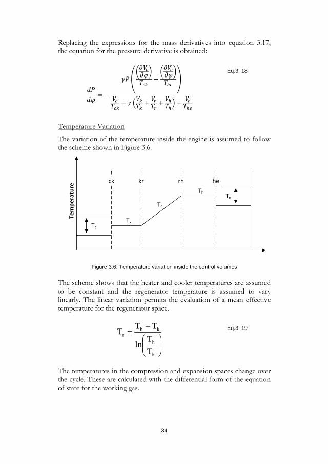
Replacing the expressions for the mass derivatives into equation 3.17, the equation for the pressure derivative is obtained:

𝑑𝑑𝑃𝑃𝑑𝑑𝜑𝜑

= −

𝛾𝛾𝑃𝑃��𝜕𝜕𝐶𝐶𝑐𝑐𝜕𝜕ϕ�𝑁𝑁𝑐𝑐𝑙𝑙

+�𝜕𝜕𝐶𝐶𝑏𝑏𝜕𝜕ϕ�𝑁𝑁ℎ𝑏𝑏

�

𝐶𝐶𝑐𝑐𝑁𝑁𝑐𝑐𝑙𝑙

+ 𝛾𝛾 �𝐶𝐶𝑙𝑙𝑁𝑁𝑙𝑙+ 𝐶𝐶𝑟𝑟𝑁𝑁𝑟𝑟

+ 𝐶𝐶ℎ𝑁𝑁ℎ� + 𝐶𝐶𝑏𝑏

𝑁𝑁ℎ𝑏𝑏

Eq.3. 18

Temperature Variation

The variation of the temperature inside the engine is assumed to follow the scheme shown in Figure 3.6.

TcTk

Tr

Th Te

Tem

pera

ture

ck kr rh he

Figure 3.6: Temperature variation inside the control volumes

The scheme shows that the heater and cooler temperatures are assumed to be constant and the regenerator temperature is assumed to vary linearly. The linear variation permits the evaluation of a mean effective temperature for the regenerator space.

−

=

k

h

khr

TTln

TTT Eq.3. 19

The temperatures in the compression and expansion spaces change over the cycle. These are calculated with the differential form of the equation of state for the working gas.

34

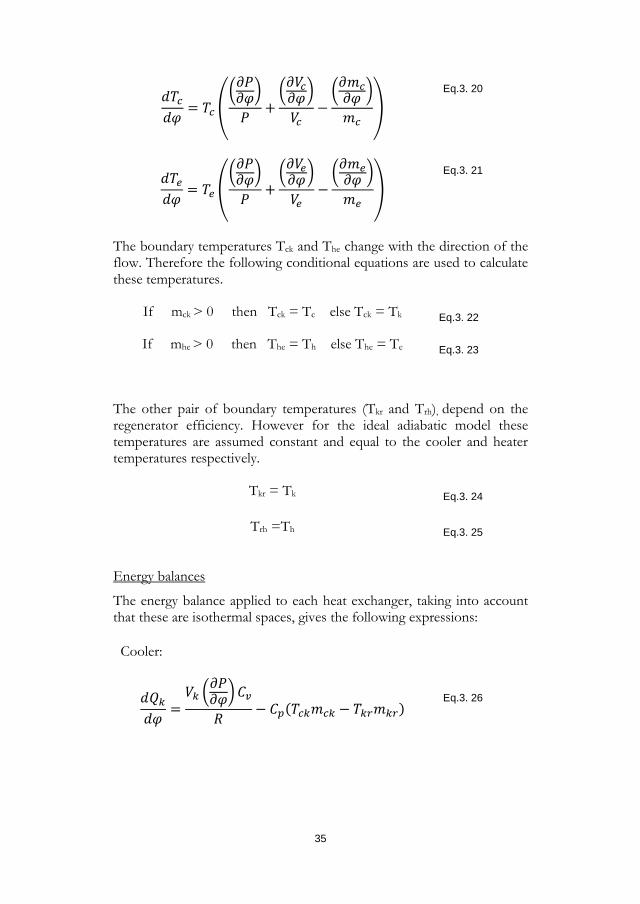
𝑑𝑑𝑁𝑁𝑐𝑐𝑑𝑑𝜑𝜑

= 𝑁𝑁𝑐𝑐 ��𝜕𝜕𝑃𝑃𝜕𝜕𝜑𝜑�

𝑃𝑃+�𝜕𝜕𝐶𝐶𝑐𝑐𝜕𝜕𝜑𝜑�

𝐶𝐶𝑐𝑐−�𝜕𝜕𝑚𝑚𝑐𝑐𝜕𝜕𝜑𝜑 �

𝑚𝑚𝑐𝑐�

Eq.3. 20

𝑑𝑑𝑁𝑁𝑏𝑏𝑑𝑑𝜑𝜑

= 𝑁𝑁𝑏𝑏 ��𝜕𝜕𝑃𝑃𝜕𝜕𝜑𝜑�

𝑃𝑃+�𝜕𝜕𝐶𝐶𝑏𝑏𝜕𝜕𝜑𝜑�

𝐶𝐶𝑏𝑏−�𝜕𝜕𝑚𝑚𝑏𝑏𝜕𝜕𝜑𝜑 �

𝑚𝑚𝑏𝑏�

Eq.3. 21

The boundary temperatures Tck and The change with the direction of the flow. Therefore the following conditional equations are used to calculate these temperatures.

If mck > 0 then Tck = Tc else Tck = Tk Eq.3. 22

If mhe > 0 then The = Th else The = Te Eq.3. 23

The other pair of boundary temperatures (Tkr and Trh), depend on the regenerator efficiency. However for the ideal adiabatic model these temperatures are assumed constant and equal to the cooler and heater temperatures respectively.

Tkr = Tk Eq.3. 24

Trh =Th Eq.3. 25

Energy balances

The energy balance applied to each heat exchanger, taking into account that these are isothermal spaces, gives the following expressions: Cooler:

𝑑𝑑𝑄𝑄𝑙𝑙𝑑𝑑𝜑𝜑

=𝐶𝐶𝑙𝑙 �

𝜕𝜕𝑃𝑃𝜕𝜕𝜑𝜑�𝐶𝐶𝑣𝑣𝑅𝑅

− 𝐶𝐶𝑣𝑣(𝑁𝑁𝑐𝑐𝑙𝑙𝑚𝑚𝑐𝑐𝑙𝑙 − 𝑁𝑁𝑙𝑙𝑟𝑟𝑚𝑚𝑙𝑙𝑟𝑟)

Eq.3. 26

35

Regenerator:

𝑑𝑑𝑄𝑄𝑟𝑟𝑑𝑑𝜑𝜑

=𝐶𝐶𝑟𝑟 �


− 𝐶𝐶𝑣𝑣(𝑁𝑁𝑙𝑙𝑟𝑟𝑚𝑚𝑙𝑙𝑟𝑟 − 𝑁𝑁𝑟𝑟ℎ𝑚𝑚𝑟𝑟ℎ)

Eq.3. 27

Heater:

𝑑𝑑𝑄𝑄ℎ𝑑𝑑𝜑𝜑

=𝐶𝐶ℎ �


− 𝐶𝐶𝑣𝑣(𝑁𝑁𝑟𝑟ℎ𝑚𝑚𝑟𝑟ℎ − 𝑁𝑁ℎ𝑏𝑏𝑚𝑚ℎ𝑏𝑏)

Eq.3. 28

Finally, the compression and expansion work are calculated from the energy balance applied to the corresponding working spaces, which are assumed adiabatic.

𝑑𝑑𝑊𝑊𝑐𝑐

𝑑𝑑𝜑𝜑= 𝑃𝑃 �

𝜕𝜕𝐶𝐶𝑐𝑐𝜕𝜕𝜑𝜑

� Eq.3. 29

𝑑𝑑𝑊𝑊𝑏𝑏

𝑑𝑑𝜑𝜑= 𝑃𝑃 �

𝜕𝜕𝐶𝐶𝑏𝑏𝜕𝜕𝜑𝜑

� Eq.3. 30

H e a t t r a n s f e r m o d u l e s 3.2.2

The adiabatic model estimates different variables in the Stirling engine. However the heat transfer characteristics are not included. For this reason, the heat transfer modules were coupled to complement the model limitations. These modules consider the thermal energy that flows, into and out of the engine. This heat flow is transferred to the working fluid via the heat exchangers at the hot and cold ends as it is shown in Figure 3.7.

36

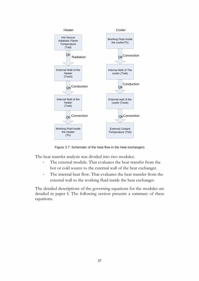
Conduction

Convection

Hot Source Adiabatic Flame

Temperature (Tad)

External Wall of the Heater(Twoh)

Internal Wall of the heater(Twih)

Radiation

Working Fluid inside the Heater

(Th)

Qh

Qh

Qh

Convection

Convection

Working Fluid inside the cooler(Tk)

Internal Wall of The cooler (Twik)

External wall of the cooler (Twok)

External Coolant Temperature (Tek)

Heater Cooler

Qk

Qk

Qk

Conduction

Figure 3.7: Schematic of the heat flow in the heat exchangers

The heat transfer analysis was divided into two modules: - The external module. That evaluates the heat transfer from the

hot or cold source to the external wall of the heat exchanger. - The internal heat flow. That evaluates the heat transfer from the

external wall to the working fluid inside the heat exchanger.

The detailed descriptions of the governing equations for the modules are detailed in paper I. The following section presents a summary of these equations.

37

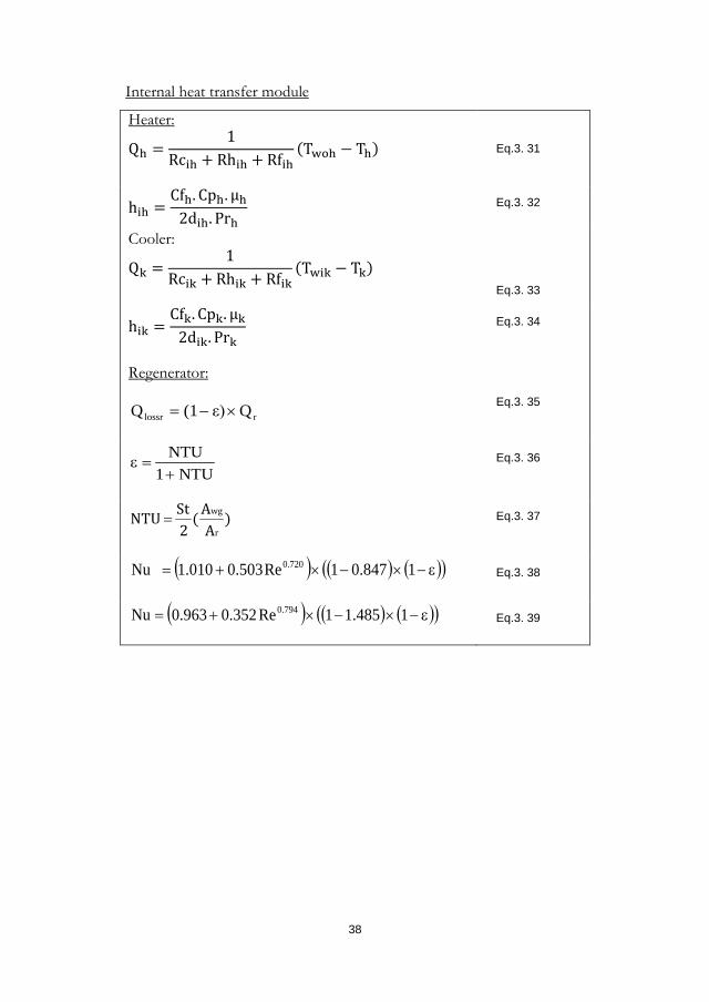
Internal heat transfer module

Heater:

Qh =1

Rcih + Rhih + Rfih(Twoh − Th)

Eq.3. 31

hih =Cfh. Cph.µh

2dih. Prh Eq.3. 32

Cooler:

Qk =1

Rcik + Rhik + Rfik(Twik − Tk)

Eq.3. 33

hik =Cfk. Cpk. µk

2dik. Prk Eq.3. 34

Regenerator:

rlossr Qε)(1Q ×−=

Eq.3. 35

NTU1NTU+

=ε Eq.3. 36

)A

A(2StNTU

r

wg= Eq.3. 37

( ) ( ) ( )( )ε−×−×+= 1847.01Re503.0010.1Nu 720.0 Eq.3. 38

( ) ( ) ( )( )ε−×−×+= 1485.11Re352.0963.0Nu 794.0 Eq.3. 39

38

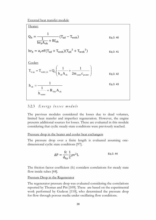
External heat transfer module

Heater:

Qh =1

1hrhAoh

+ Rfoh(Tad − Twoh)

Eq.3. 40

hrh = αrσF(Tad + Twoh)(Tad2 + Twoh2)

Eq.3. 41

Cooler:

++=

pwaterwaterokokkwater_inokw c2m

1Ah1QTT

Eq.3. 42

okfokwater

ok

ARh

11h

+= Eq.3. 43

E n e r g y l o s s e s m o d u l e 3.2.3

The previous modules considered the losses due to dead volumes, limited heat transfer and imperfect regeneration. However, the engine presents additional sources for losses. These are evaluated in this module considering that cyclic steady-state conditions were previously reached. Pressure drop in the heater and cooler heat exchangers

The pressure drop over a finite length is evaluated assuming one-dimensional cyclic state conditions [97].

∆P =fc

dhy12ρv2L Eq.3. 44

The friction factor coefficient (fc) considers correlations for steady state flow inside tubes [44].

Pressure Drop in the Regenerator

The regenerator pressure drop was evaluated considering the correlations reported by Thomas and Pitt [109]. These are based on the experimental work performed by Gedeon [110], who determined the pressure drop for flow through porous media under oscillating flow conditions.

39

The following expression is considered:

∆P = Cfnρ2

v2 Eq.3. 45

From this expression, the pressure drop is proportional to the number of flow resistors (n), the square of the mean velocity (v2) and the friction coefficient (Cf). The friction coefficient considers the form drag (Cfd) and skin friction (Csf) factors.

ReC

CC sffdf += Eq.3. 46

Total losses due to pressure drop

The total pressure drop is evaluated by the sum of the losses at each heat exchanger during the complete cycle.

Wploss = � ��∆Pi

i=3

i=1

dVedφ

�2π

0dφ

Eq.3. 47

Losses due to internal conduction

The conductive losses represent the axial heat transfer due to the difference of temperature along the heat exchangers. The following expression was considered [15] :

)T(TLAkQ wikwih

r

rrlk −= Eq.3. 48

Losses due to shuttle conduction

Shuttle conduction occurs due to the oscillation of the hot displacer across a temperature gradient. The displacer absorbs the heat at the hot end of its stroke and then released it at the cold end. This is estimated with the following expression [111].

40

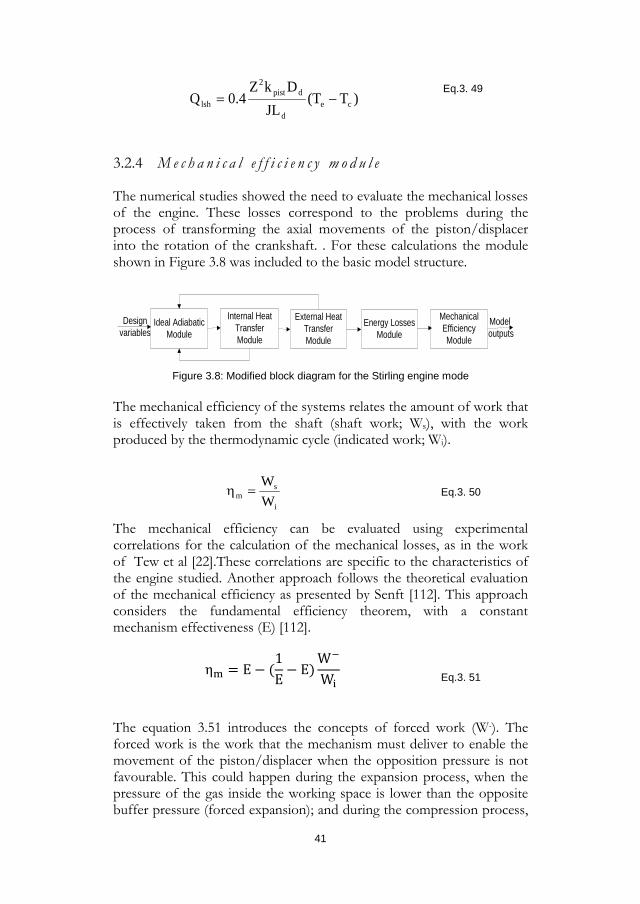
)T(TJL

DkZ0.4Q ce

d

dpist2

lsh −= Eq.3. 49

M e c h a n i c a l e f f i c i e n c y m o d u l e 3.2.4

The numerical studies showed the need to evaluate the mechanical losses of the engine. These losses correspond to the problems during the process of transforming the axial movements of the piston/displacer into the rotation of the crankshaft. . For these calculations the module shown in Figure 3.8 was included to the basic model structure.

Ideal Adiabatic Module

Internal Heat Transfer Module

External Heat Transfer Module

Energy Losses Module

Design variables

Model outputs

Mechanical Efficiency Module

Figure 3.8: Modified block diagram for the Stirling engine mode

The mechanical efficiency of the systems relates the amount of work that is effectively taken from the shaft (shaft work; Ws), with the work produced by the thermodynamic cycle (indicated work; Wi).

i

sm W

W=η Eq.3. 50

The mechanical efficiency can be evaluated using experimental correlations for the calculation of the mechanical losses, as in the work of Tew et al [22].These correlations are specific to the characteristics of the engine studied. Another approach follows the theoretical evaluation of the mechanical efficiency as presented by Senft [112]. This approach considers the fundamental efficiency theorem, with a constant mechanism effectiveness (E) [112].

ηm = E − (1E− E)

W−

Wi Eq.3. 51

The equation 3.51 introduces the concepts of forced work (W-). The forced work is the work that the mechanism must deliver to enable the movement of the piston/displacer when the opposition pressure is not favourable. This could happen during the expansion process, when the pressure of the gas inside the working space is lower than the opposite buffer pressure (forced expansion); and during the compression process,

41

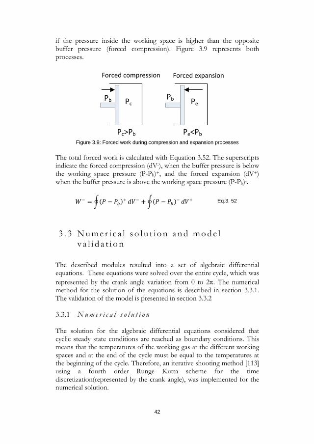
if the pressure inside the working space is higher than the opposite buffer pressure (forced compression). Figure 3.9 represents both processes.

Pc

Forced compression

Pb

Pc>Pb

Pe

Pe<Pb

Forced expansion

Pb

Figure 3.9: Forced work during compression and expansion processes

The total forced work is calculated with Equation 3.52. The superscripts indicate the forced compression (dV-), when the buffer pressure is below the working space pressure (P-Pb)+, and the forced expansion (dV+) when the buffer pressure is above the working space pressure (P-Pb)-.

𝑊𝑊− = �(𝑃𝑃 − 𝑃𝑃𝑏𝑏)+ 𝑑𝑑𝐶𝐶− + �(𝑃𝑃 − 𝑃𝑃𝑏𝑏)− 𝑑𝑑𝐶𝐶+ Eq.3. 52

3 . 3 N u m e r i c a l s o l u t i o n a n d m o d e l v a l i d a t i o n

The described modules resulted into a set of algebraic differential equations. These equations were solved over the entire cycle, which was represented by the crank angle variation from 0 to 2π. The numerical method for the solution of the equations is described in section 3.3.1. The validation of the model is presented in section 3.3.2

N u m e r i c a l s o l u t i o n 3.3.1

The solution for the algebraic differential equations considered that cyclic steady state conditions are reached as boundary conditions. This means that the temperatures of the working gas at the different working spaces and at the end of the cycle must be equal to the temperatures at the beginning of the cycle. Therefore, an iterative shooting method [113] using a fourth order Runge Kutta scheme for the time discretization(represented by the crank angle), was implemented for the numerical solution.

42

The iterative process assumed that the initial values are known, and then the system is solved until cyclic steady state conditions, which was numerically reached when the difference between the assumed initial values and the values calculated at the end of the cycle are lower than a defined error. Once the cyclic steady state solution was reached, the energy losses and the forced work were evaluated. The forced work was calculated from Equation 3.52 using the classical Simpson 3/8 numerical integration rule [114].

The numerical solution was implemented in Aspen Custom Modeller (ACM), but an external C++ procedure was coupled to implement the shooting method. The scheme described in Figure 3.10 represents the described methodology.

43

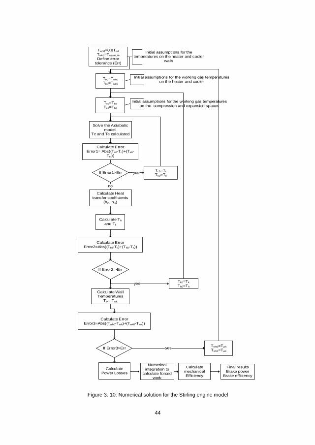
Twh0=0.8TadTwk0=Twater_inDefine error

tolerance (Err)

Th0=Twh0Tk0=Twk0

Tc0=Tk0Te0=Th0

Solve the Adiabatic model.

Tc and Te calculated

Calculate ErrorError1= Abs((Tc0-Tc)+(Te0-

Tef))

If Error1>Err Tc0=TcTe0=Te

yes

Calculate Heat transfer coefficients

(hih, hik)

no

Calculate Th and Tk

Calculate Error Error2=Abs((Tk0-Tk)+(Th0-Th))

If Error2 >Err

Tk0=TkTh0=Th

Calculate Wall Temperatures

Twh, Twk

yes

Calculate ErrorError3=Abs((Twh0-Twh)+(Twk0-Twk))

If Error3>Err Twh0=TwhTwk0=Twk

yes

Calculate Power Losses

Initial assumptions for the temperatures on the heater and cooler

walls

Initial assumptions for the working gas temperatures on the heater and cooler

Initial assumptions for the working gas temperatures on the compression and expansion spaces

Numerical integration to

calculate forced work

Calculate mechanical Efficiency

Final results Brake power

Brake efficiency

Figure 3. 10: Numerical solution for the Stirling engine model

44

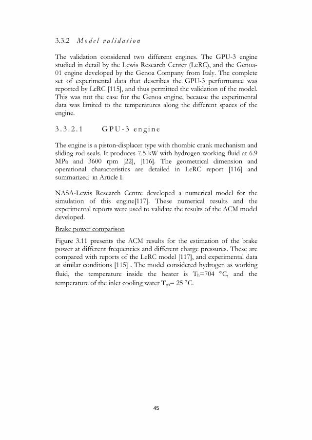
M o d e l v a l i d a t i o n 3.3.2

The validation considered two different engines. The GPU-3 engine studied in detail by the Lewis Research Center (LeRC), and the Genoa-01 engine developed by the Genoa Company from Italy. The complete set of experimental data that describes the GPU-3 performance was reported by LeRC [115], and thus permitted the validation of the model. This was not the case for the Genoa engine, because the experimental data was limited to the temperatures along the different spaces of the engine.

3 . 3 . 2 . 1 G P U - 3 e n g i n e

The engine is a piston-displacer type with rhombic crank mechanism and sliding rod seals. It produces 7.5 kW with hydrogen working fluid at 6.9 MPa and 3600 rpm [22], [116]. The geometrical dimension and operational characteristics are detailed in LeRC report [116] and summarized in Article I.

NASA-Lewis Research Centre developed a numerical model for the simulation of this engine[117]. These numerical results and the experimental reports were used to validate the results of the ACM model developed.

Brake power comparison

Figure 3.11 presents the ACM results for the estimation of the brake power at different frequencies and different charge pressures. These are compared with reports of the LeRC model [117], and experimental data at similar conditions [115] . The model considered hydrogen as working fluid, the temperature inside the heater is Th=704 °C, and the temperature of the inlet cooling water Twi= 25 °C.

45

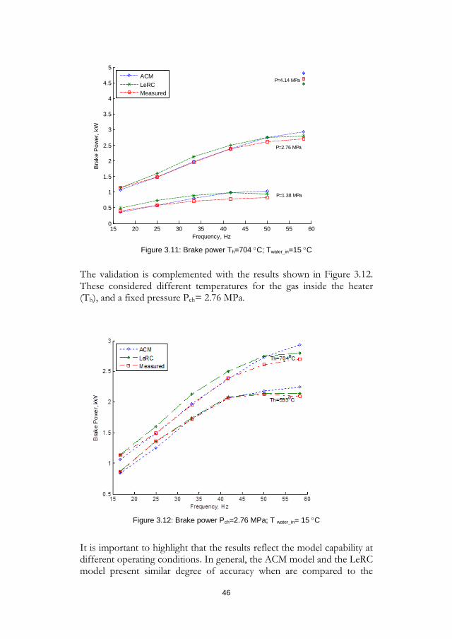
Figure 3.11: Brake power Th=704 °C; Twater_in=15 °C

The validation is complemented with the results shown in Figure 3.12. These considered different temperatures for the gas inside the heater (Th), and a fixed pressure Pch= 2.76 MPa.

Figure 3.12: Brake power Pch=2.76 MPa; T water_in= 15 °C

It is important to highlight that the results reflect the model capability at different operating conditions. In general, the ACM model and the LeRC model present similar degree of accuracy when are compared to the

15 20 25 30 35 40 45 50 55 600

0.5

1

1.5

2

2.5

3

3.5

4

4.5

5

Frequency, Hz

Bra

ke P

ower

, kW

ACMLeRCMeasured

P=1.38 MPa

P=2.76 MPa

P=4.14 MPa

46

experimental data. The ACM model presents better estimations at low and intermediate pressures and low frequencies. The relative error for the ACM model at intermediate pressure and low frequencies is around ±5%, but this tends to increase to ±8% at higher frequencies. On the other hand, the LeRC model present better accuracy at higher frequencies and lower temperatures.

In general, both models presented limitations for the calculations of the losses through the engine. These calculations were based on correlations, which could be improved with calibrations at the particular conditions of the flow through the engine. The ACM model pretended to better capture these losses including correlation for oscillating flow conditions. This may explain the better accuracy at low and medium frequencies, where the oscillating conditions are more relevant. On the other hand, the LeRC model was based in the use of more control volumes, and thus captures better the variation of the gas properties along the engine. This is shown in the better capability at high temperatures and high frequencies.

Brake efficiency comparison

Figure 3.13 presents the brake efficiency comparison between the ACM, LeRC models and the measured data. These results reflect the difficulty that both models present for the estimation of the real heat input, and the different losses through the engine. These differences can be explained by the indirect methodology for the evaluation of the heat input presented on the experimental reports. This methodology assumed ideal combustion conditions for a hot energy balance and thus the experimental results presented a higher intrinsic error. Despite of the mentioned difficulties, the ACM model presents good estimations at different pressure level and frequencies. At intermediate pressure, the maximum error was reported as ±14% at a frequency of 16.67 Hz, at higher frequencies the errors were reported around ±8%. The estimation at lower pressure was more difficult, the results shown the underestimation of the brake power at the different frequencies. On the other hand, the estimation at higher pressure P=4.14 MPa was better. These results may reflect the use of the correlations that aim to capture the oscillating flow conditions for the evaluation of heat transfer and pressure drop through the regenerator. However, a better calibration of the correlations may improve the calculations for the efficiency.

47

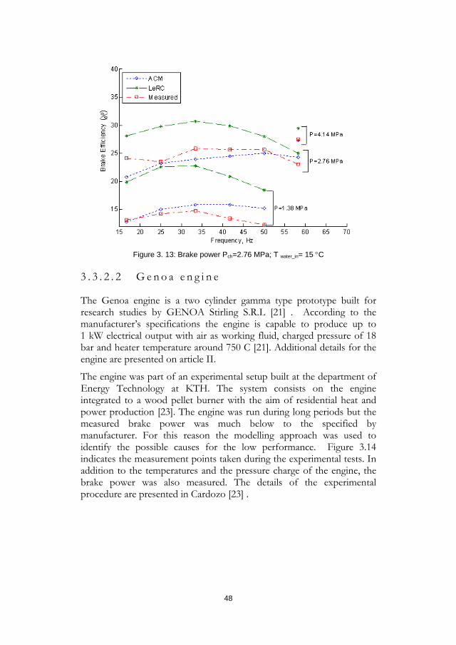
Figure 3. 13: Brake power Pch=2.76 MPa; T water_in= 15 °C

3 . 3 . 2 . 2 G e n o a e n g i n e

The Genoa engine is a two cylinder gamma type prototype built for research studies by GENOA Stirling S.R.L [21] . According to the manufacturer’s specifications the engine is capable to produce up to 1 kW electrical output with air as working fluid, charged pressure of 18 bar and heater temperature around 750 C [21]. Additional details for the engine are presented on article II.

The engine was part of an experimental setup built at the department of Energy Technology at KTH. The system consists on the engine integrated to a wood pellet burner with the aim of residential heat and power production [23]. The engine was run during long periods but the measured brake power was much below to the specified by manufacturer. For this reason the modelling approach was used to identify the possible causes for the low performance. Figure 3.14 indicates the measurement points taken during the experimental tests. In addition to the temperatures and the pressure charge of the engine, the brake power was also measured. The details of the experimental procedure are presented in Cardozo [23] .

48

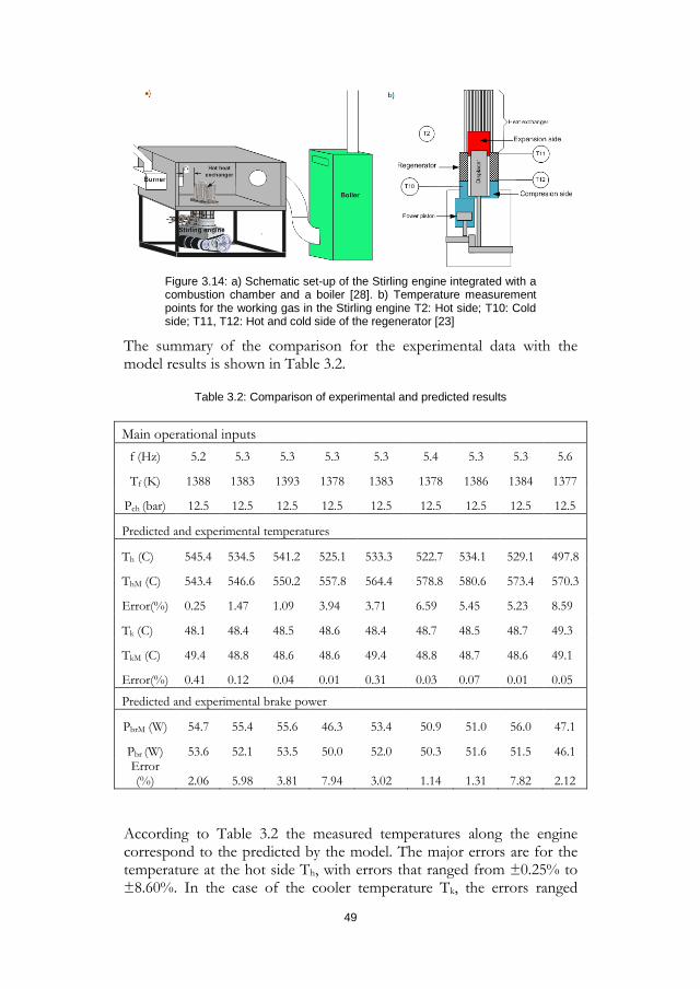
Figure 3.14: a) Schematic set-up of the Stirling engine integrated with a combustion chamber and a boiler [28]. b) Temperature measurement points for the working gas in the Stirling engine T2: Hot side; T10: Cold side; T11, T12: Hot and cold side of the regenerator [23]

The summary of the comparison for the experimental data with the model results is shown in Table 3.2.

Table 3.2: Comparison of experimental and predicted results

Main operational inputs f (Hz) 5.2 5.3 5.3 5.3 5.3 5.4 5.3 5.3 5.6

Tf (K) 1388 1383 1393 1378 1383 1378 1386 1384 1377

Pch (bar) 12.5 12.5 12.5 12.5 12.5 12.5 12.5 12.5 12.5

Predicted and experimental temperatures

Th (C) 545.4 534.5 541.2 525.1 533.3 522.7 534.1 529.1 497.8

ThM (C) 543.4 546.6 550.2 557.8 564.4 578.8 580.6 573.4 570.3

Error(%) 0.25 1.47 1.09 3.94 3.71 6.59 5.45 5.23 8.59

Tk (C) 48.1 48.4 48.5 48.6 48.4 48.7 48.5 48.7 49.3

TkM (C) 49.4 48.8 48.6 48.6 49.4 48.8 48.7 48.6 49.1

Error(%) 0.41 0.12 0.04 0.01 0.31 0.03 0.07 0.01 0.05

Predicted and experimental brake power

PbrM (W) 54.7 55.4 55.6 46.3 53.4 50.9 51.0 56.0 47.1

Pbr (W) 53.6 52.1 53.5 50.0 52.0 50.3 51.6 51.5 46.1 Error (%) 2.06 5.98 3.81 7.94 3.02 1.14 1.31 7.82 2.12

According to Table 3.2 the measured temperatures along the engine correspond to the predicted by the model. The major errors are for the temperature at the hot side Th, with errors that ranged from ±0.25% to ±8.60%. In the case of the cooler temperature Tk, the errors ranged

49

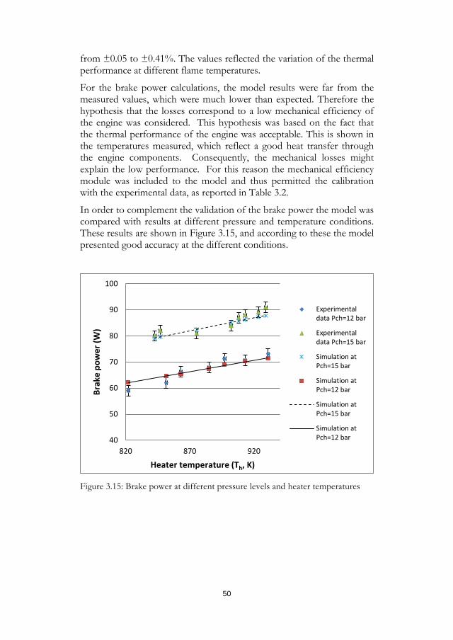
from ±0.05 to ±0.41%. The values reflected the variation of the thermal performance at different flame temperatures.

For the brake power calculations, the model results were far from the measured values, which were much lower than expected. Therefore the hypothesis that the losses correspond to a low mechanical efficiency of the engine was considered. This hypothesis was based on the fact that the thermal performance of the engine was acceptable. This is shown in the temperatures measured, which reflect a good heat transfer through the engine components. Consequently, the mechanical losses might explain the low performance. For this reason the mechanical efficiency module was included to the model and thus permitted the calibration with the experimental data, as reported in Table 3.2.

In order to complement the validation of the brake power the model was compared with results at different pressure and temperature conditions. These results are shown in Figure 3.15, and according to these the model presented good accuracy at the different conditions.

Figure 3.15: Brake power at different pressure levels and heater temperatures

40

50

60

70

80

90

100

820 870 920

Brak

e po

wer

(W)

Heater temperature (Th, K)

Experimentaldata Pch=12 bar

Experimentaldata Pch=15 bar

Simulation atPch=15 bar




50

3 . 4 C o n c l u s i o n s o f t h e c h a p t e r

The main contribution presented in this chapter is the development of a mathematical model that included the heat transfer phenomena, thermodynamics, and mechanical efficiency interactions to describe the operation of Stirling engine systems. This integrated approach permits the variation of different parameters that may affect the engine performance and thus represent a valuable tool for design assessment.

The validity of the model was probed with the comparison against two different engine prototypes. The simulations for the GPU-3 engine presented good accuracy when compared with the experimental reports. In the case of the Genoa engine the validation was more challenging, because the engine presented low experimental performances. For this reasons the concept of mechanical efficiency and forced work were included to explain these results.

In general the model capability was good enough for design assessments. However, the accuracy for the simulation of a specific engine can be improved by updating the model with experimental correlations obtained for a specific case study.

51

52

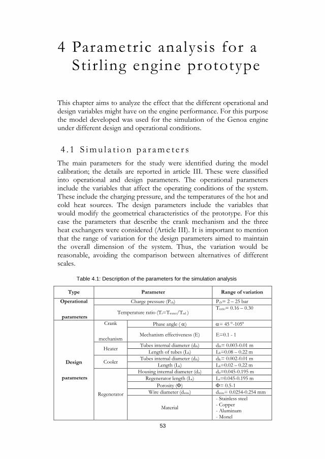
4 Parametric analysis for a Stir l ing engine prototype

This chapter aims to analyze the effect that the different operational and design variables might have on the engine performance. For this purpose the model developed was used for the simulation of the Genoa engine under different design and operational conditions.

4 . 1 S i m u l a t i o n p a r a m e t e r s The main parameters for the study were identified during the model calibration; the details are reported in article III. These were classified into operational and design parameters. The operational parameters include the variables that affect the operating conditions of the system. These include the charging pressure, and the temperatures of the hot and cold heat sources. The design parameters include the variables that would modify the geometrical characteristics of the prototype. For this case the parameters that describe the crank mechanism and the three heat exchangers were considered (Article III). It is important to mention that the range of variation for the design parameters aimed to maintain the overall dimension of the system. Thus, the variation would be reasonable, avoiding the comparison between alternatives of different scales.

Table 4.1: Description of the parameters for the simulation analysis

Type Parameter Range of variation

Operational

parameters

Charge pressure (Pch) Pch= 2 – 25 bar

Temperature ratio (Tr=Twater/Tad ) Tratio= 0.16 – 0.30

Design

parameters

Crank

mechanism

Phase angle ( α) α= 45 °-105°

Mechanism effectiveness (E) E=0.1 - 1

Heater Tubes internal diameter (dih) dih= 0.003-0.01 m Length of tubes (Lh) Lh=0.08 – 0.22 m

Cooler Tubes internal diameter (dik) dik= 0.002-0.01 m Length (Lk) Lk=0.02 – 0.22 m

Regenerator

Housing internal diameter (dir) dir=0.045-0.195 m Regenerator length (Lr) Lr=0.045-0.195 m

Porosity (Φ) Φ= 0.5-1 Wire diameter (dwire) dwire= 0.0254-0.254 mm

Material

- Stainless steel - Copper - Aluminum - Monel

53

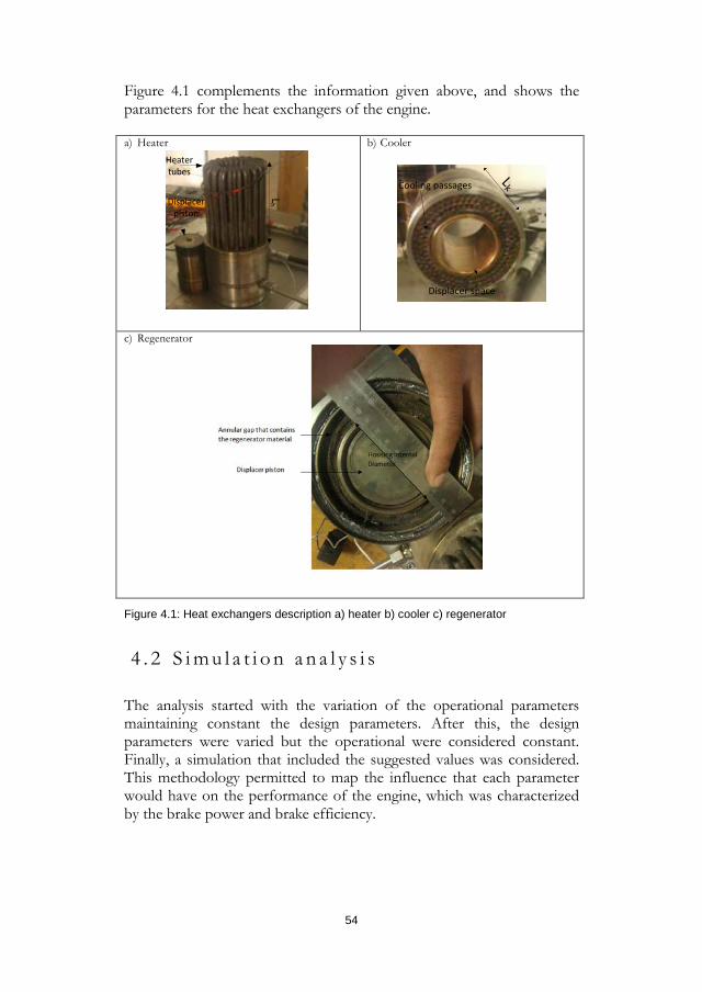
Figure 4.1 complements the information given above, and shows the parameters for the heat exchangers of the engine.

a) Heater

Lh

Heater tubes

Displacer piston

b) Cooler

Cooling passages Lk

Displacer space

c) Regenerator

Figure 4.1: Heat exchangers description a) heater b) cooler c) regenerator

4 . 2 S i m u l a t i o n a n a l y s i s

The analysis started with the variation of the operational parameters maintaining constant the design parameters. After this, the design parameters were varied but the operational were considered constant. Finally, a simulation that included the suggested values was considered. This methodology permitted to map the influence that each parameter would have on the performance of the engine, which was characterized by the brake power and brake efficiency.

54

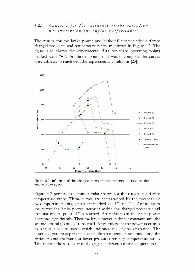
A n a l y s i s f o r t h e i n f l u e n c e o f t h e o p e r a t i o n 4.2.1p a r a m e t e r s o n t h e e n g i n e p e r f o r m a n c e

The results for the brake power and brake efficiency under different charged pressures and temperature ratios are shown in Figure 4.2. The figure also shows the experimental data for three operating points marked with “♦”. Additional points that would complete the curves were difficult to reach with the experimental conditions [23].

Figure 4.2: Influence of the charged pressure and temperature ratio on the engine brake power

Figure 4.2 permits to identify similar shapes for the curves at different temperature ratios. These curves are characterized by the presence of two important points, which are marked as “1” and “2”. According to the curves the brake power increases within the charged pressure until the first critical point “1” is reached. After this point the brake power decreases significantly .Then the brake power is almost constant until the second critical point “2” is reached. After this point the power decreases to values close to zero, which indicates no engine operation. The described pattern is presented at the different temperature ratios, and the critical points are found at lower pressures for high temperature ratios. This reflects the sensibility of the engine at lower hot side temperatures.

0

20

40

60

80

100

120

0 5 10 15 20 25 30

Brak

e po

wer

(W)

Charged pressure (bar)

Tratio=0.30

Tratio=0.21

Tratio=0.20

Tratio=0.19

Tratio=0.16

operating point

measured brakepower

1

2

1

2

55

The described patterns reflect the two conflictive effects that the charged pressure have on the engine. The first is a positive effect, because the increment of the pressure level increases the mass of the working gas and thus the power output. However, the second effect is negative because it also increased the mean buffer pressure in the system. According to the fundamental efficiency theorem, represented by equations 3.51 and 3.52, the buffer pressure would increase the forced work and thus reduce the brake power output. Therefore, the point “1” would represent the point where the negative increased forced work is higher than the potential increment of the brake power. The second critical point “2” may reflect the imbalance between the heat input to the engine and the brake power at the higher operation pressures. This means that the heat into the engine is not enough to operate the system.

Figure 4.2 also shows the positive influence that lowering the temperature ratio would have on the brake power. The reduction implies higher flame temperatures on the hot side and thus is limited only by the properties of the heater material.

A n a l y s i s f o r t h e i n f l u e n c e o f t h e d e s i g n 4.2.2p a r a m e t e r s o n t h e e n g i n e p e r f o r m a n c e

This section presents numerical results for the simulation of the engine considering the design parameters, for the crank mechanism and the three heat exchangers, shown in table 4.1. The operational conditions were assumed fixed during the variation of the geometrical parameters.

4 . 2 . 2 . 1 C r a n k m e c h a n i s m

Different mechanism arrangements were described in the section 2.1. This section analyzes two common parameters that guide the design of these mechanisms: The phase angle (α), and the mechanism effectiveness (E). The first parameter determines the dynamics of the piston-displacer movements and thus the volume variation during the cycle. The second parameter measures the amount of cyclic thermodynamic work converted into brake power as explained in section 3.2.4. It is important to mention that the detailed design of the crank mechanism is not covered in the study.

The results for the brake power and brake efficiency considering the variation of the crank parameters are shown in Figure 4.3. The operation conditions were maintained constant and closer to the optimum values determined in the previous section: Pch=22 bar Tratio = 0.16.

56

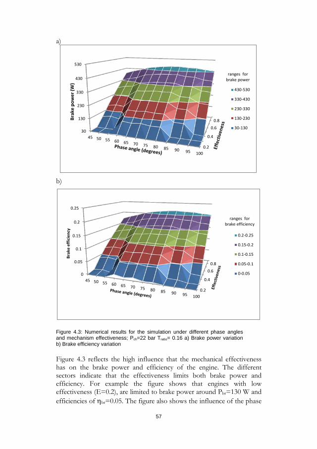
a)

b)

Figure 4.3: Numerical results for the simulation under different phase angles and mechanism effectiveness; Pch=22 bar Tratio= 0.16 a) Brake power variation b) Brake efficiency variation

Figure 4.3 reflects the high influence that the mechanical effectiveness has on the brake power and efficiency of the engine. The different sectors indicate that the effectiveness limits both brake power and efficiency. For example the figure shows that engines with low effectiveness (E=0.2), are limited to brake power around Pbr=130 W and efficiencies of ηbr=0.05. The figure also shows the influence of the phase

0.2

0.4

0.6

0.8

30

130

230

330

430

530

45 50 55 60 65 70 75 80 85 90 95 100

Brak

e po

wer

(W)

430-530

330-430

230-330

130-230

30-130

ranges for brake power

0.2

0.4

0.60.8

0

0.05

0.1

0.15

0.2

0.25

45 50 55 60 65 70 75 80 85 90 95 100

Brak

e ef

ficie

ncy

0.2-0.25

0.15-0.2

0.1-0.15

0.05-0.1

0-0.05

ranges for brake efficiency

57

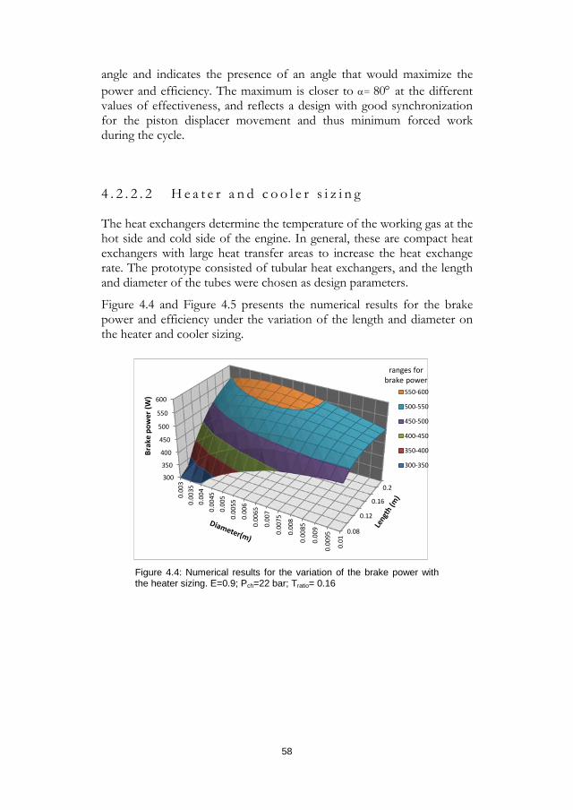
angle and indicates the presence of an angle that would maximize the power and efficiency. The maximum is closer to α= 80° at the different values of effectiveness, and reflects a design with good synchronization for the piston displacer movement and thus minimum forced work during the cycle.

4 . 2 . 2 . 2 H e a t e r a n d c o o l e r s i z i n g

The heat exchangers determine the temperature of the working gas at the hot side and cold side of the engine. In general, these are compact heat exchangers with large heat transfer areas to increase the heat exchange rate. The prototype consisted of tubular heat exchangers, and the length and diameter of the tubes were chosen as design parameters.

Figure 4.4 and Figure 4.5 presents the numerical results for the brake power and efficiency under the variation of the length and diameter on the heater and cooler sizing.

Figure 4.4: Numerical results for the variation of the brake power with the heater sizing. E=0.9; Pch=22 bar; Tratio= 0.16

0.08

0.12

0.16

0.2300

350

400

450

500

550

600

0.00

30.

0035

0.00

40.

0045

0.00

50.

0055

0.00

60.

0065

0.00

7

0.00

75

0.00

8

0.00

85

0.00

9

0.00

95

0.01

Brak

e po

wer

(W) 550-600

500-550

450-500

400-450

350-400

300-350

ranges for brake power

58

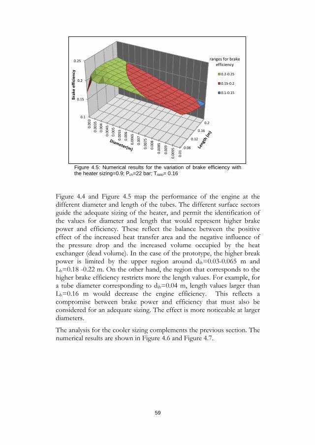
Figure 4.5: Numerical results for the variation of brake efficiency with the heater sizing=0.9; Pch=22 bar; Tratio= 0.16

Figure 4.4 and Figure 4.5 map the performance of the engine at the different diameter and length of the tubes. The different surface sectors guide the adequate sizing of the heater, and permit the identification of the values for diameter and length that would represent higher brake power and efficiency. These reflect the balance between the positive effect of the increased heat transfer area and the negative influence of the pressure drop and the increased volume occupied by the heat exchanger (dead volume). In the case of the prototype, the higher break power is limited by the upper region around dih=0.03-0.065 m and Lh=0.18 -0.22 m. On the other hand, the region that corresponds to the higher brake efficiency restricts more the length values. For example, for a tube diameter corresponding to dih=0.04 m, length values larger than Lh=0.16 m would decrease the engine efficiency. This reflects a compromise between brake power and efficiency that must also be considered for an adequate sizing. The effect is more noticeable at larger diameters.

The analysis for the cooler sizing complements the previous section. The numerical results are shown in Figure 4.6 and Figure 4.7.

0.08

0.12

0.16

0.20.1

0.15

0.2

0.25

0.00

30.

0035

0.00

40.

0045

0.00

5

0.00

55

0.00

6

0.00

65

0.00

7

0.00

75

0.00

8

0.00

85

0.00

9

0.00

95

0.01

Brak

e ef

ficie

ncy

0.2-0.25

0.15-0.2

0.1-0.15

ranges for brake efficiency

59

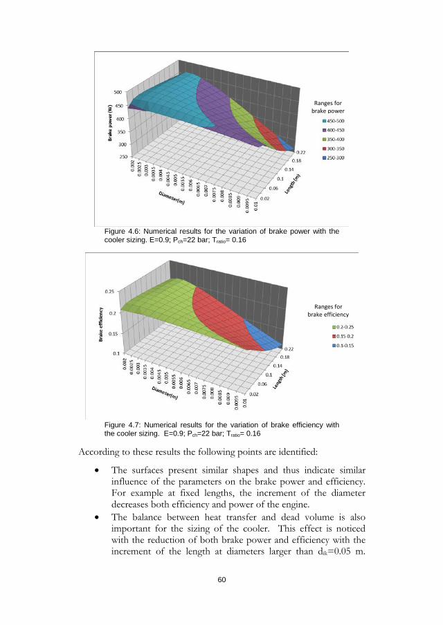
Figure 4.6: Numerical results for the variation of brake power with the cooler sizing. E=0.9; Pch=22 bar; Tratio= 0.16

Figure 4.7: Numerical results for the variation of brake efficiency with the cooler sizing. E=0.9; Pch=22 bar; Tratio= 0.16

According to these results the following points are identified:

• The surfaces present similar shapes and thus indicate similar influence of the parameters on the brake power and efficiency. For example at fixed lengths, the increment of the diameter decreases both efficiency and power of the engine.

• The balance between heat transfer and dead volume is also important for the sizing of the cooler. This effect is noticed with the reduction of both brake power and efficiency with the increment of the length at diameters larger than dik=0.05 m.

Ranges for brake power

Ranges for brake efficiency

60

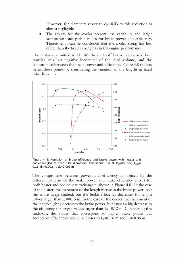
However, for diameters closer to dik=0.03 m this reduction is almost negligible.

• The results for the cooler present less variability and larger sectors with acceptable values for brake power and efficiency. Therefore, it can be concluded that the cooler sizing has less effect than the heater sizing has in the engine performance.

The analysis permitted to identify the trade-off between increased heat transfer area but negative increment of the dead volume, and the compromise between the brake power and efficiency. Figure 4.8 reflects better these points by considering the variation of the lengths at fixed tube diameters.

Figure 4. 8: Variation of brake efficiency and brake power with heater and cooler lengths at fixed tube diameters. Conditions: E=0.9; Pch=22 bar; Tratio= 0.16; dih=0.003 m; dik=0.003 m

The compromise between power and efficiency is noticed by the different patterns of the brake power and brake efficiency curves for both heater and cooler heat exchangers, shown in Figure 4.8. In the case of the heater, the increment of the length increases the brake power over the entire range studied, but the brake efficiency decreases for length values larger than Lh=0.15 m. In the case of the cooler, the increment of the length slightly decreases the brake power, but causes a big decrease in the efficiency for length values larger than Lk=0.12 m. Considering this trade-off, the values that correspond to higher brake power but acceptable efficiencies would be closer to Lh=0.16 m and Lk= 0.06 m.

61

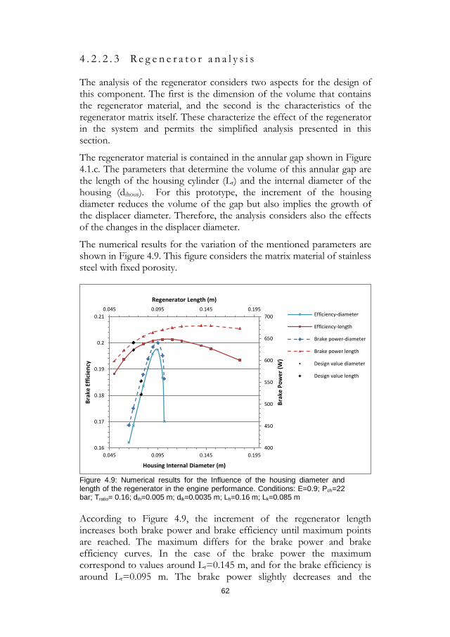
4 . 2 . 2 . 3 R e g e n e r a t o r a n a l y s i s

The analysis of the regenerator considers two aspects for the design of this component. The first is the dimension of the volume that contains the regenerator material, and the second is the characteristics of the regenerator matrix itself. These characterize the effect of the regenerator in the system and permits the simplified analysis presented in this section.

The regenerator material is contained in the annular gap shown in Figure 4.1.c. The parameters that determine the volume of this annular gap are the length of the housing cylinder (Lr) and the internal diameter of the housing (dihous). For this prototype, the increment of the housing diameter reduces the volume of the gap but also implies the growth of the displacer diameter. Therefore, the analysis considers also the effects of the changes in the displacer diameter.

The numerical results for the variation of the mentioned parameters are shown in Figure 4.9. This figure considers the matrix material of stainless steel with fixed porosity.

Figure 4.9: Numerical results for the Influence of the housing diameter and length of the regenerator in the engine performance. Conditions: E=0.9; Pch=22 bar; Tratio= 0.16; dih=0.005 m; dik=0.0035 m; Lh=0.16 m; Lk=0.085 m

According to Figure 4.9, the increment of the regenerator length increases both brake power and brake efficiency until maximum points are reached. The maximum differs for the brake power and brake efficiency curves. In the case of the brake power the maximum correspond to values around Lr=0.145 m, and for the brake efficiency is around Lr=0.095 m. The brake power slightly decreases and the

0.045 0.095 0.145 0.195

400

450

500

550

600

650

700

0.16

0.17

0.18

0.19

0.2

0.21

0.045 0.095 0.145 0.195

Regenerator Length (m)

Brak

e Po

wer

(W)

Brak

e Ef

ficie

ncy

Housing Internal Diameter (m)

Efficiency-diameter

Efficiency-length

Brake power-diameter

Brake power length

Design value diameter

Design value length

62

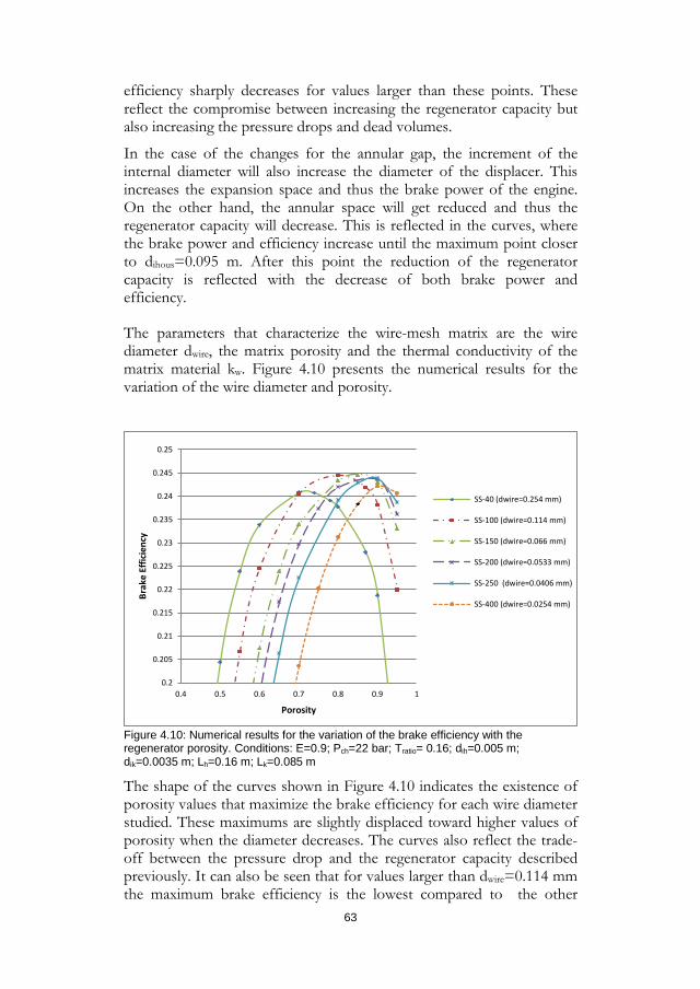
efficiency sharply decreases for values larger than these points. These reflect the compromise between increasing the regenerator capacity but also increasing the pressure drops and dead volumes.

In the case of the changes for the annular gap, the increment of the internal diameter will also increase the diameter of the displacer. This increases the expansion space and thus the brake power of the engine. On the other hand, the annular space will get reduced and thus the regenerator capacity will decrease. This is reflected in the curves, where the brake power and efficiency increase until the maximum point closer to dihous=0.095 m. After this point the reduction of the regenerator capacity is reflected with the decrease of both brake power and efficiency.

The parameters that characterize the wire-mesh matrix are the wire diameter dwire, the matrix porosity and the thermal conductivity of the matrix material kw. Figure 4.10 presents the numerical results for the variation of the wire diameter and porosity.

Figure 4.10: Numerical results for the variation of the brake efficiency with the regenerator porosity. Conditions: E=0.9; Pch=22 bar; Tratio= 0.16; dih=0.005 m; dik=0.0035 m; Lh=0.16 m; Lk=0.085 m

The shape of the curves shown in Figure 4.10 indicates the existence of porosity values that maximize the brake efficiency for each wire diameter studied. These maximums are slightly displaced toward higher values of porosity when the diameter decreases. The curves also reflect the trade-off between the pressure drop and the regenerator capacity described previously. It can also be seen that for values larger than dwire=0.114 mm the maximum brake efficiency is the lowest compared to the other

0.2

0.205

0.21

0.215

0.22

0.225

0.23

0.235

0.24

0.245

0.25

0.4 0.5 0.6 0.7 0.8 0.9 1

Brak

e Ef

ficie

ncy

Porosity

SS-40 (dwire=0.254 mm)

SS-100 (dwire=0.114 mm)

SS-150 (dwire=0.066 mm)

SS-200 (dwire=0.0533 mm)

SS-250 (dwire=0.0406 mm)

SS-400 (dwire=0.0254 mm)

63

cases. In general, a correspondence between porosity and wire diameter must be considered for the matrix dimensions.

In the case of the matrix thermal conductivity, the results showed an almost negligible sensitivity for the changes in this parameter. For this reason, a qualitative analysis based on the work of Gheith et al [118] was done. This experimental work evaluated materials with different thermal conductivities: Stainless steel (SS), copper, aluminium and monel.

In general, the regenerator material must have: good capacity to store and release the heat to the working fluid;low axial conductivity to reduce the axial conduction losses; and material resistance to high temperatures. Therefore, according to the results of Gheith et al [118] , the use of stainless steel for the matrix was suggested over other materials.


The main contribution shown on this chapter was the demonstration of the proposed model for the study of Stirling engines under realistic design and operational conditions. The advantage of the model is the integrated thermodynamic, thermal and mechanical analysis. This approach allowed to identify compromises between different design aspects, and allowed to obtain curves that mapped the engine performance under different conditions.

The results of the analysis are summarized in the following points:

• The variation of the charged pressures and temperature ratios allowed to obtain performance curves, which were characterized by two critical points. The first point represents the negative influence that an increased forced work would have on the engine performance. The second point may reflect the imbalance between the heat input and the brake power at higher operational pressures.

• The analysis of the crank mechanism showed that the phase angle around α= 80° would maximize the engine performance. In addition, the influence that the mechanism effectiveness has on the brake power and efficiency of the engine was demonstrated.

• The analysis of the heater and cooler sizing reflected a compromise between dead volumes and increase heat transfer area. In the case of the heater, the increment of the length increases the brake power over the entire range studied, but the brake efficiency starts to decrease after a critical length value. In the case of the cooler, a critical

64

cooler length was also identified. For values larger than this critical length, there is slightly decrease on the brake power and a large decrease on the brake efficiency.

• The regenerator analysis reflected the compromise between the positive increment of the regenerator capacity and the negative increased pressure drop and dead volume. For the annular regenerator the influence on the power output was also analyzed. The analysis presented curves with a maximum point that represents the adequate balance of the mentioned variables.

• The analysis for the regenerator mesh reflected the large influence of the porosity on the performance. Furthermore, the need for a correspondence between porosity and wire diameter was identified

• The simulation results revealed two conflictive design objectives: the design towards increased power output, and the design towards engines with high efficiency. The design priority should depend on the engine applications. For example, in the case of CHP systems the design of engines with higher brake power is more relevant because the thermal energy is recovered at additional heat exchangers.

65

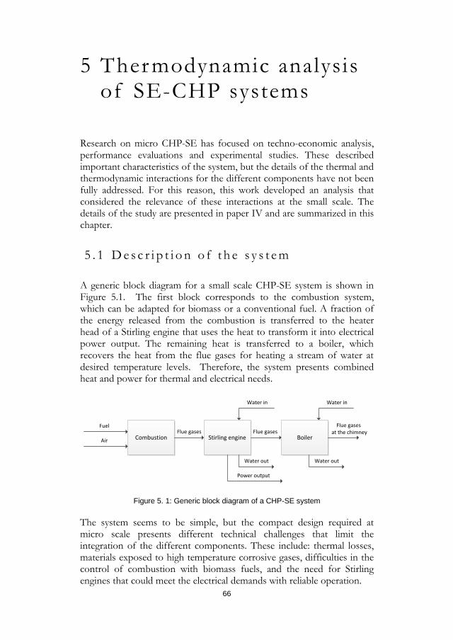
5 Thermodynamic analysis of SE-CHP systems

Research on micro CHP-SE has focused on techno-economic analysis, performance evaluations and experimental studies. These described important characteristics of the system, but the details of the thermal and thermodynamic interactions for the different components have not been fully addressed. For this reason, this work developed an analysis that considered the relevance of these interactions at the small scale. The details of the study are presented in paper IV and are summarized in this chapter.

5 . 1 D e s c r i p t i o n o f t h e s y s t e m

A generic block diagram for a small scale CHP-SE system is shown in Figure 5.1. The first block corresponds to the combustion system, which can be adapted for biomass or a conventional fuel. A fraction of the energy released from the combustion is transferred to the heater head of a Stirling engine that uses the heat to transform it into electrical power output. The remaining heat is transferred to a boiler, which recovers the heat from the flue gases for heating a stream of water at desired temperature levels. Therefore, the system presents combined heat and power for thermal and electrical needs.

Combustion

Fuel

AirFlue gases

Stirling engine BoilerFlue gases

Flue gases at the chimney

Water in

Water out

Water in

Water out

Power output

Figure 5. 1: Generic block diagram of a CHP-SE system

The system seems to be simple, but the compact design required at micro scale presents different technical challenges that limit the integration of the different components. These include: thermal losses, materials exposed to high temperature corrosive gases, difficulties in the control of combustion with biomass fuels, and the need for Stirling engines that could meet the electrical demands with reliable operation.

66

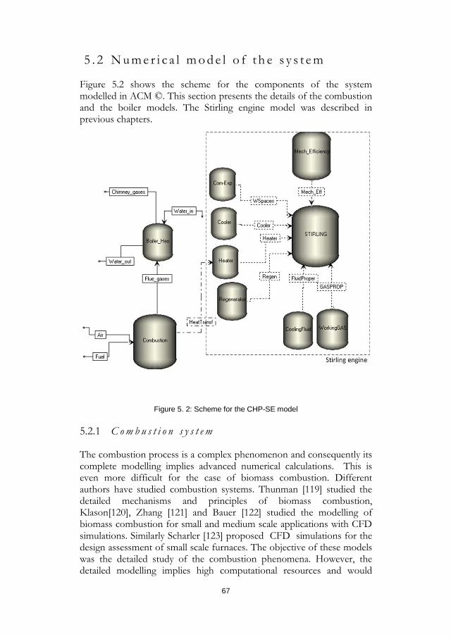
5 . 2 N u m e r i c a l m o d e l o f t h e s y s t e m

Figure 5.2 shows the scheme for the components of the system modelled in ACM ©. This section presents the details of the combustion and the boiler models. The Stirling engine model was described in previous chapters.

Figure 5. 2: Scheme for the CHP-SE model

C o m b u s t i o n s y s t e m 5.2.1

The combustion process is a complex phenomenon and consequently its complete modelling implies advanced numerical calculations. This is even more difficult for the case of biomass combustion. Different authors have studied combustion systems. Thunman [119] studied the detailed mechanisms and principles of biomass combustion, Klason[120], Zhang [121] and Bauer [122] studied the modelling of biomass combustion for small and medium scale applications with CFD simulations. Similarly Scharler [123] proposed CFD simulations for the design assessment of small scale furnaces. The objective of these models was the detailed study of the combustion phenomena. However, the detailed modelling implies high computational resources and would

67

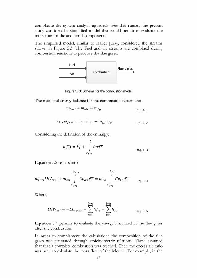
complicate the system analysis approach. For this reason, the present study considered a simplified model that would permit to evaluate the interaction of the additional components.

The simplified model, similar to Haller [124], considered the streams shown in Figure 5.3. The Fuel and air streams are combined during combustion reactions to produce the flue gases.

Combustion

Fuel

AirFlue gases

Figure 5. 3: Scheme for the combustion model

The mass and energy balance for the combustion system are:

𝑚𝑚𝑓𝑓𝑓𝑓𝑏𝑏𝑏𝑏 + 𝑚𝑚𝑚𝑚𝑚𝑚𝑟𝑟 = 𝑚𝑚𝑓𝑓𝑓𝑓 Eq. 5. 1

𝑚𝑚𝑓𝑓𝑓𝑓𝑏𝑏𝑏𝑏ℎ𝑓𝑓𝑓𝑓𝑏𝑏𝑏𝑏 + 𝑚𝑚𝑚𝑚𝑚𝑚𝑟𝑟ℎ𝑚𝑚𝑚𝑚𝑟𝑟 = 𝑚𝑚𝑓𝑓𝑓𝑓 ℎ𝑓𝑓𝑓𝑓 Eq. 5. 2

Considering the definition of the enthalpy:

ℎ(𝑁𝑁) = ℎ�̇�𝐻 + � 𝐶𝐶𝐶𝐶𝑑𝑑𝑁𝑁𝑇𝑇

𝑇𝑇𝑟𝑟𝑟𝑟𝑟𝑟

Eq. 5. 3

Equation 5.2 results into:

𝑚𝑚𝑓𝑓𝑓𝑓𝑏𝑏𝑏𝑏𝐿𝐿𝐻𝐻𝐶𝐶𝑓𝑓𝑓𝑓𝑏𝑏𝑏𝑏 + 𝑚𝑚𝑚𝑚𝑚𝑚𝑟𝑟 � 𝐶𝐶𝐶𝐶𝑚𝑚𝑚𝑚𝑟𝑟𝑑𝑑𝑁𝑁

𝑇𝑇𝑎𝑎𝑎𝑎𝑟𝑟


= 𝑚𝑚𝑓𝑓𝑓𝑓 � 𝐶𝐶𝐶𝐶𝑓𝑓𝑓𝑓𝑑𝑑𝑁𝑁

𝑇𝑇𝑟𝑟𝑓𝑓


Eq. 5. 4

Where,

𝐿𝐿𝐻𝐻𝐶𝐶𝑓𝑓𝑓𝑓𝑏𝑏𝑏𝑏 = −∆𝐻𝐻𝑐𝑐𝑏𝑏𝑚𝑚𝑏𝑏 = �ℎ̇𝐻𝐻𝑟𝑟𝑐𝑐

𝑚𝑚=𝑚𝑚

𝑚𝑚=1

−�ℎ̇𝐻𝐻𝑣𝑣

𝑚𝑚=𝑚𝑚

𝑚𝑚=1

Eq. 5. 5

Equation 5.4 permits to evaluate the energy contained in the flue gases after the combustion.

In order to complement the calculations the composition of the flue gases was estimated through stoichiometric relations. These assumed that that a complete combustion was reached. Then the excess air ratio was used to calculate the mass flow of the inlet air. For example, in the

68

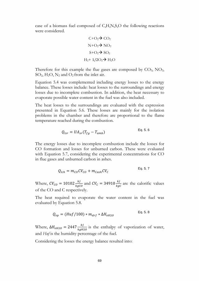
case of a biomass fuel composed of C,H,N,S,O the following reactions were considered.

C+O2 CO2

N+O2 NO2

S+O2 SO2

H2+ 1/2O2 H2O

Therefore for this example the flue gases are composed by CO2, NO2, SO2, H2O, N2 and O2 from the inlet air.

Equation 5.4 was complemented including energy losses to the energy balance. These losses include: heat losses to the surroundings and energy losses due to incomplete combustion. In addition, the heat necessary to evaporate possible water content in the fuel was also included.

The heat losses to the surroundings are evaluated with the expression presented in Equation 5.6. These losses are mainly for the isolation problems in the chamber and therefore are proportional to the flame temperature reached during the combustion.

𝑄𝑄𝑏𝑏𝑠𝑠𝑟𝑟 = 𝑁𝑁𝐴𝐴𝑠𝑠𝑟𝑟(𝑁𝑁𝑓𝑓𝑓𝑓 − 𝑁𝑁𝑚𝑚𝑚𝑚𝑏𝑏) Eq. 5. 6

The energy losses due to incomplete combustion include the losses for CO formation and losses for unburned carbon. These were evaluated with Equation 5.7, considering the experimental concentrations for CO in flue gases and unburned carbon in ashes.

𝑄𝑄𝑏𝑏𝑐𝑐ℎ = 𝑚𝑚𝐶𝐶𝑂𝑂𝐶𝐶𝐶𝐶𝐶𝐶𝑂𝑂 + 𝑚𝑚𝐶𝐶𝑚𝑚𝑠𝑠ℎ𝐶𝐶𝐶𝐶𝐶𝐶 Eq. 5. 7

Where, 𝐶𝐶𝐶𝐶𝐶𝐶𝑂𝑂 = 10102 𝑙𝑙𝑘𝑘𝑙𝑙𝑓𝑓𝐶𝐶𝑂𝑂

and 𝐶𝐶𝐶𝐶𝐶𝐶 = 34910 𝑙𝑙𝑘𝑘𝑙𝑙𝑓𝑓𝐶𝐶

are the calorific values of the CO and C respectively. The heat required to evaporate the water content in the fuel was evaluated by Equation 5.8.

𝑄𝑄𝑣𝑣𝑣𝑣 = (𝐻𝐻𝐻𝐻𝐻𝐻/100) ∗ 𝑚𝑚𝑓𝑓𝑟𝑟𝑓𝑓 ∗ ∆𝐻𝐻𝑣𝑣𝑣𝑣2𝑂𝑂 Eq. 5. 8

Where, ∆𝐻𝐻𝑣𝑣𝑣𝑣2𝑂𝑂 = 2447 𝑙𝑙𝑘𝑘𝑙𝑙𝑓𝑓𝑣𝑣2𝑂𝑂

is the enthalpy of vaporization of water, and Huf is the humidity percentage of the fuel. Considering the losses the energy balance resulted into:

69

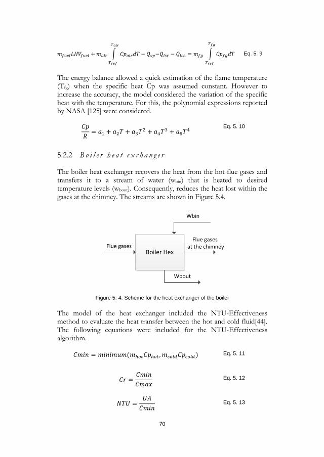
𝑚𝑚𝑓𝑓𝑓𝑓𝑏𝑏𝑏𝑏𝐿𝐿𝐻𝐻𝐶𝐶𝑓𝑓𝑓𝑓𝑏𝑏𝑏𝑏 +𝑚𝑚𝑚𝑚𝑚𝑚𝑟𝑟 � 𝐶𝐶𝐶𝐶𝑚𝑚𝑚𝑚𝑟𝑟𝑑𝑑𝑁𝑁

𝑇𝑇𝑎𝑎𝑎𝑎𝑟𝑟


− 𝑄𝑄𝑣𝑣𝑣𝑣−𝑄𝑄𝑏𝑏𝑠𝑠𝑟𝑟 − 𝑄𝑄𝑏𝑏𝑐𝑐ℎ = 𝑚𝑚𝑓𝑓𝑓𝑓 � 𝐶𝐶𝐶𝐶𝑓𝑓𝑓𝑓𝑑𝑑𝑁𝑁

𝑇𝑇𝑟𝑟𝑓𝑓


Eq. 5. 9

The energy balance allowed a quick estimation of the flame temperature (Tfg) when the specific heat Cp was assumed constant. However to increase the accuracy, the model considered the variation of the specific heat with the temperature. For this, the polynomial expressions reported by NASA [125] were considered.

𝐶𝐶𝐶𝐶𝑅𝑅

= 𝑎𝑎1 + 𝑎𝑎2𝑁𝑁 + 𝑎𝑎3𝑁𝑁2 + 𝑎𝑎4𝑁𝑁3 + 𝑎𝑎5𝑁𝑁4 Eq. 5. 10

B o i l e r h e a t e x c h a n g e r 5.2.2

The boiler heat exchanger recovers the heat from the hot flue gases and transfers it to a stream of water (wbin) that is heated to desired temperature levels (wbout). Consequently, reduces the heat lost within the gases at the chimney. The streams are shown in Figure 5.4.

Boiler HexFlue gases

Flue gases at the chimney

Wbin

Wbout

Figure 5. 4: Scheme for the heat exchanger of the boiler

The model of the heat exchanger included the NTU-Effectiveness method to evaluate the heat transfer between the hot and cold fluid[44]. The following equations were included for the NTU-Effectiveness algorithm.

𝐶𝐶𝑚𝑚𝑤𝑤𝑤𝑤 = 𝑚𝑚𝑤𝑤𝑤𝑤𝑤𝑤𝑚𝑚𝐻𝐻𝑚𝑚(𝑚𝑚ℎ𝑏𝑏𝑜𝑜𝐶𝐶𝐶𝐶ℎ𝑏𝑏𝑜𝑜 ,𝑚𝑚𝑐𝑐𝑏𝑏𝑏𝑏𝑓𝑓𝐶𝐶𝐶𝐶𝑐𝑐𝑏𝑏𝑏𝑏𝑓𝑓) Eq. 5. 11

𝐶𝐶𝑟𝑟 =𝐶𝐶𝑚𝑚𝑤𝑤𝑤𝑤𝐶𝐶𝑚𝑚𝑎𝑎𝑥𝑥

Eq. 5. 12

𝑁𝑁𝑁𝑁𝑁𝑁 =𝑁𝑁𝐴𝐴𝐶𝐶𝑚𝑚𝑤𝑤𝑤𝑤

Eq. 5. 13

70

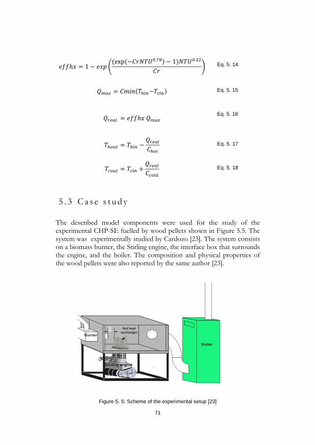
𝑅𝑅𝐻𝐻𝐻𝐻ℎ𝑥𝑥 = 1 − 𝑅𝑅𝑥𝑥𝐶𝐶 �(exp(−𝐶𝐶𝑟𝑟𝑁𝑁𝑁𝑁𝑁𝑁0.78) − 1)𝑁𝑁𝑁𝑁𝑁𝑁0.22

𝐶𝐶𝑟𝑟� Eq. 5. 14

𝑄𝑄𝑚𝑚𝑚𝑚𝑚𝑚 = 𝐶𝐶𝑚𝑚𝑤𝑤𝑤𝑤(𝑁𝑁ℎ𝑚𝑚𝑚𝑚−𝑁𝑁𝑐𝑐𝑚𝑚𝑚𝑚) Eq. 5. 15

𝑄𝑄𝑟𝑟𝑏𝑏𝑚𝑚𝑏𝑏 = 𝑅𝑅𝐻𝐻𝐻𝐻ℎ𝑥𝑥 𝑄𝑄𝑚𝑚𝑚𝑚𝑚𝑚 Eq. 5. 16

𝑁𝑁ℎ𝑏𝑏𝑓𝑓𝑜𝑜 = 𝑁𝑁ℎ𝑚𝑚𝑚𝑚 −𝑄𝑄𝑟𝑟𝑏𝑏𝑚𝑚𝑏𝑏𝐶𝐶ℎ𝑏𝑏𝑜𝑜

Eq. 5. 17

𝑁𝑁𝑐𝑐𝑏𝑏𝑓𝑓𝑜𝑜 = 𝑁𝑁𝑐𝑐𝑚𝑚𝑚𝑚 +𝑄𝑄𝑟𝑟𝑏𝑏𝑚𝑚𝑏𝑏𝐶𝐶𝑐𝑐𝑏𝑏𝑏𝑏𝑓𝑓

Eq. 5. 18

5 . 3 C a s e s t u d y

The described model components were used for the study of the experimental CHP-SE fuelled by wood pellets shown in Figure 5.5. The system was experimentally studied by Cardozo [23]. The system consists on a biomass burner, the Stirling engine, the interface box that surrounds the engine, and the boiler. The composition and physical properties of the wood pellets were also reported by the same author [23].

Figure 5. 5: Scheme of the experimental setup [23]

71

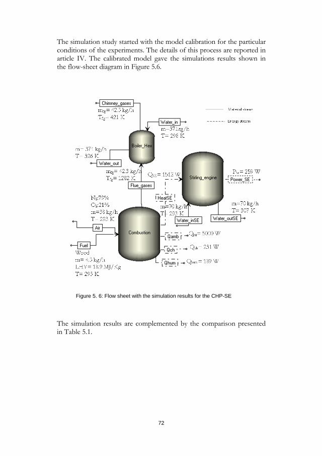
The simulation study started with the model calibration for the particular conditions of the experiments. The details of this process are reported in article IV. The calibrated model gave the simulations results shown in the flow-sheet diagram in Figure 5.6.

Figure 5. 6: Flow sheet with the simulation results for the CHP-SE

The simulation results are complemented by the comparison presented in Table 5.1.

72

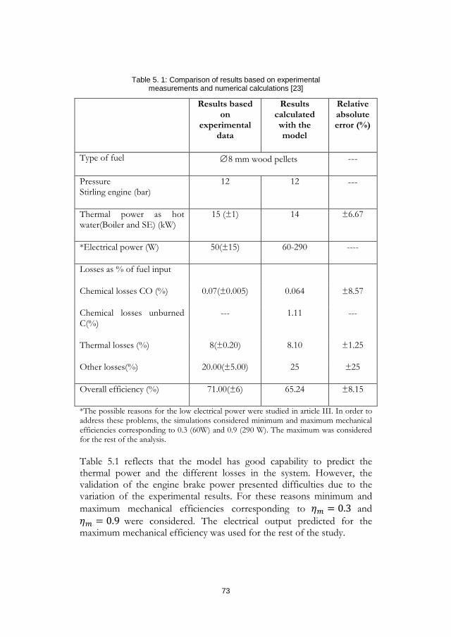
Table 5. 1: Comparison of results based on experimental measurements and numerical calculations [23]

Results based on

experimental data

Results calculated with the model

Relative absolute error (%)

Type of fuel ∅8 mm wood pellets ---

Pressure Stirling engine (bar)

12 12 ---

Thermal power as hot water(Boiler and SE) (kW)

15 (±1) 14 ±6.67

*Electrical power (W) 50(±15) 60-290 ----

Losses as % of fuel input

Chemical losses CO (%) 0.07(±0.005) 0.064 ±8.57

Chemical losses unburned C(%)

--- 1.11 ---

Thermal losses (%) 8(±0.20) 8.10 ±1.25

Other losses(%) 20.00(±5.00) 25 ±25

Overall efficiency (%) 71.00(±6) 65.24 ±8.15

*The possible reasons for the low electrical power were studied in article III. In order to address these problems, the simulations considered minimum and maximum mechanical efficiencies corresponding to 0.3 (60W) and 0.9 (290 W). The maximum was considered for the rest of the analysis.

Table 5.1 reflects that the model has good capability to predict the thermal power and the different losses in the system. However, the validation of the engine brake power presented difficulties due to the variation of the experimental results. For these reasons minimum and maximum mechanical efficiencies corresponding to 𝜂𝜂𝑚𝑚 = 0.3 and 𝜂𝜂𝑚𝑚 = 0.9 were considered. The electrical output predicted for the maximum mechanical efficiency was used for the rest of the study.

73

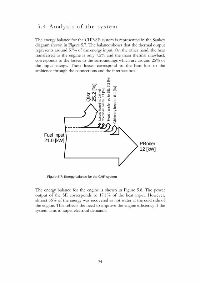
5 . 4 A n a l y s i s o f t h e s y s t e m

The energy balance for the CHP-SE system is represented in the Sankey diagram shown in Figure 5.7. The balance shows that the thermal output represents around 57% of the energy input. On the other hand, the heat transferred to the engine is only 7.2% and the main thermal drawback corresponds to the losses to the surroundings which are around 25% of the input energy. These losses correspond to the heat lost to the ambience through the connections and the interface box.

Figure 5.7: Energy balance for the CHP system

The energy balance for the engine is shown in Figure 5.8. The power output of the SE corresponds to 17.1% of the heat input. However, almost 66% of the energy was recovered as hot water at the cold side of the engine. This reflects the need to improve the engine efficiency if the system aims to target electrical demands.

Fuel Input21.0 [kW]

Qls

r25

.2 [%

]Lo

sses

hum

idity

: 0.9

[%]

Che

mic

al L

osse

s: 1

.1 [%

]

Hea

t tra

nsfe

rred

to S

E: 7

.2 [%

]

Chi

mne

y lo

sses

: 8.1

[%]

PBoiler12 [kW]

74

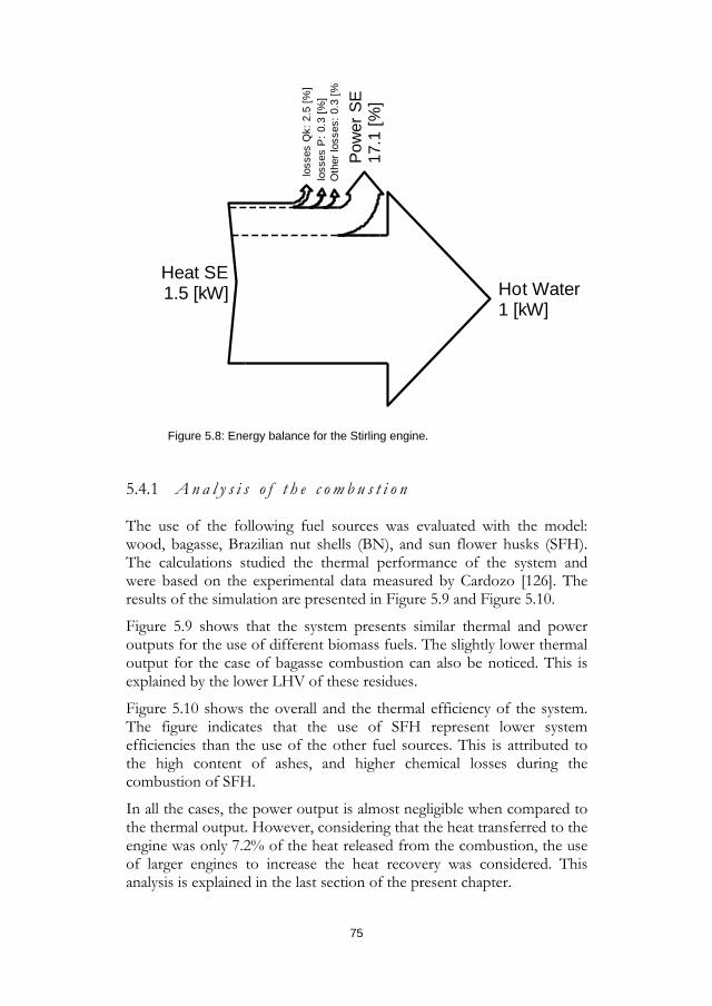
Figure 5.8: Energy balance for the Stirling engine.

A n a l y s i s o f t h e c o m b u s t i o n 5.4.1

The use of the following fuel sources was evaluated with the model: wood, bagasse, Brazilian nut shells (BN), and sun flower husks (SFH). The calculations studied the thermal performance of the system and were based on the experimental data measured by Cardozo [126]. The results of the simulation are presented in Figure 5.9 and Figure 5.10.

Figure 5.9 shows that the system presents similar thermal and power outputs for the use of different biomass fuels. The slightly lower thermal output for the case of bagasse combustion can also be noticed. This is explained by the lower LHV of these residues.

Figure 5.10 shows the overall and the thermal efficiency of the system. The figure indicates that the use of SFH represent lower system efficiencies than the use of the other fuel sources. This is attributed to the high content of ashes, and higher chemical losses during the combustion of SFH.

In all the cases, the power output is almost negligible when compared to the thermal output. However, considering that the heat transferred to the engine was only 7.2% of the heat released from the combustion, the use of larger engines to increase the heat recovery was considered. This analysis is explained in the last section of the present chapter.

Heat SE1.5 [kW]

loss

es Q

k: 2

.5 [%

]lo

sses

P: 0

.3 [%

]O

ther

loss

es: 0

.3 [%

]

Pow

er S

E 17

.1 [%

]

Hot Water1 [kW]

75

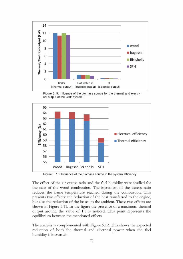
Figure 5. 9: Influence of the biomass source for the thermal and electri-cal output of the CHP system.

Figure 5. 10: Influence of the biomass source in the system efficiency

The effect of the air excess ratio and the fuel humidity were studied for the case of the wood combustion. The increment of the excess ratio reduces the flame temperature reached during the combustion. This presents two effects: the reduction of the heat transferred to the engine, but also the reduction of the losses to the ambient. These two effects are shown in Figure 5.11. In the figure the presence of a maximum thermal output around the value of 1.8 is noticed. This point represents the equilibrium between the mentioned effects.

The analysis is complemented with Figure 5.12. This shows the expected reduction of both the thermal and electrical power when the fuel humidity is increased.

0

2

4

6

8

10

12

14

Boiler(Thermal output)

Hot water SE(Thermal output)

SE(Electrical output)

Ther

mal

/Ele

ctric

al o

utpu

t (kW

)

wood

bagasse

BN shells

SFH

5556575859606162636465

Wood Bagasse BN shells SFH

Effic

ienc

y (%

)

Electrical efficiency

Thermal efficiency

76

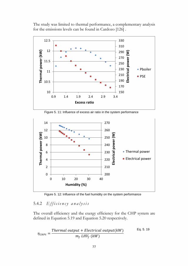
The study was limited to thermal performance, a complementary analysis for the emissions levels can be found in Cardozo [126] .

Figure 5. 11: Influence of excess air ratio in the system performance

Figure 5. 12: Influence of the fuel humidity on the system performance

E f f i c i e n c y a n a l y s i s 5.4.2

The overall efficiency and the exergy efficiency for the CHP system are defined in Equation 5.19 and Equation 5.20 respectively.

𝜂𝜂𝐶𝐶𝑣𝑣𝐶𝐶𝑜𝑜 =𝑁𝑁ℎ𝑅𝑅𝑟𝑟𝑚𝑚𝑎𝑎𝑙𝑙 𝑤𝑤𝐻𝐻𝑆𝑆𝐶𝐶𝐻𝐻𝑆𝑆 + 𝐸𝐸𝑙𝑙𝑅𝑅𝑅𝑅𝑆𝑆𝑟𝑟𝑤𝑤𝑅𝑅𝑎𝑎𝑙𝑙 𝑤𝑤𝐻𝐻𝑆𝑆𝐶𝐶𝐻𝐻𝑆𝑆(𝑘𝑘𝑊𝑊)

𝑚𝑚𝑓𝑓 𝐿𝐿𝐻𝐻𝐶𝐶𝑓𝑓 (𝑘𝑘𝑊𝑊)

Eq. 5. 19

150

170

190

210

230

250

270

290

310

330

10

10.5

11

11.5

12

12.5

0.9 1.4 1.9 2.4 2.9 3.4

Elec

tric

al p

ower

(W)

Ther

mal

pow

er (k

W)

Excess ratio

Pboiler

PSE

200

210

220

230

240

250

260

270

0

2

4

6

8

10

12

14

0 10 20 30 40

Elec

tric

al p

ower

(W)

Ther

mal

pow

er (k

W)

Humidity (%)

Thermal power

Electrical power

77

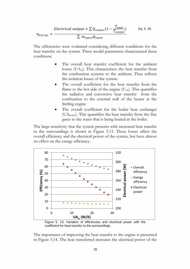
𝜂𝜂𝐸𝐸𝑚𝑚𝑏𝑏𝑟𝑟𝑓𝑓𝑦𝑦 =𝐸𝐸𝑙𝑙𝑅𝑅𝑅𝑅𝑆𝑆𝑟𝑟𝑤𝑤𝑅𝑅𝑎𝑎𝑙𝑙 𝑤𝑤𝐻𝐻𝑆𝑆𝐶𝐶𝐻𝐻𝑆𝑆 + ∑𝑄𝑄𝑏𝑏𝑓𝑓𝑜𝑜𝑣𝑣𝑓𝑓𝑜𝑜(1 − 𝑁𝑁𝑚𝑚𝑚𝑚𝑏𝑏

𝑁𝑁𝑏𝑏𝑓𝑓𝑜𝑜𝑣𝑣𝑓𝑓𝑜𝑜)

∑ 𝑚𝑚𝑚𝑚𝑚𝑚𝑣𝑣𝑓𝑓𝑜𝑜𝜓𝜓𝑚𝑚𝑚𝑚𝑣𝑣𝑓𝑓𝑜𝑜

Eq. 5. 20

The efficiencies were evaluated considering different conditions for the heat transfer on the system. Three model parameters characterized these conditions:

• The overall heat transfer coefficient for the ambient losses (UAsr). This characterizes the heat transfer from the combustion systems to the ambient. Thus reflects the isolation losses of the system.

• The overall coefficient for the heat transfer from the flame to the hot side of the engine (Uoh). This quantifies the radiative and convective heat transfer from the combustion to the external wall of the heater at the Stirling engine

• The overall coefficient for the boiler heat exchanger (UAboiler). This quantifies the heat transfer from the flue gases to the water that is being heated at the boiler.

The large sensitivity that the system presents with increased heat transfer to the surroundings is shown in Figure 5.13. These losses affect the overall efficiency and the electrical power of the system, but have almost no effect on the exergy efficiency.

Figure 5. 13: Variation of efficiencies and electrical power with the coefficient for heat transfer to the surroundings.

The importance of improving the heat transfer to the engine is presented in Figure 5.14. The heat transferred increases the electrical power of the

200

220

240

260

280

300

320

0

10

20

30

40

50

60

70

80

0 10 20 30

Elec

tric

al p

ower

(W)

Effic

ienc

y (%

)

UAsr (W/K)

OverallefficiencyExergyefficiencyElectricalpower

78

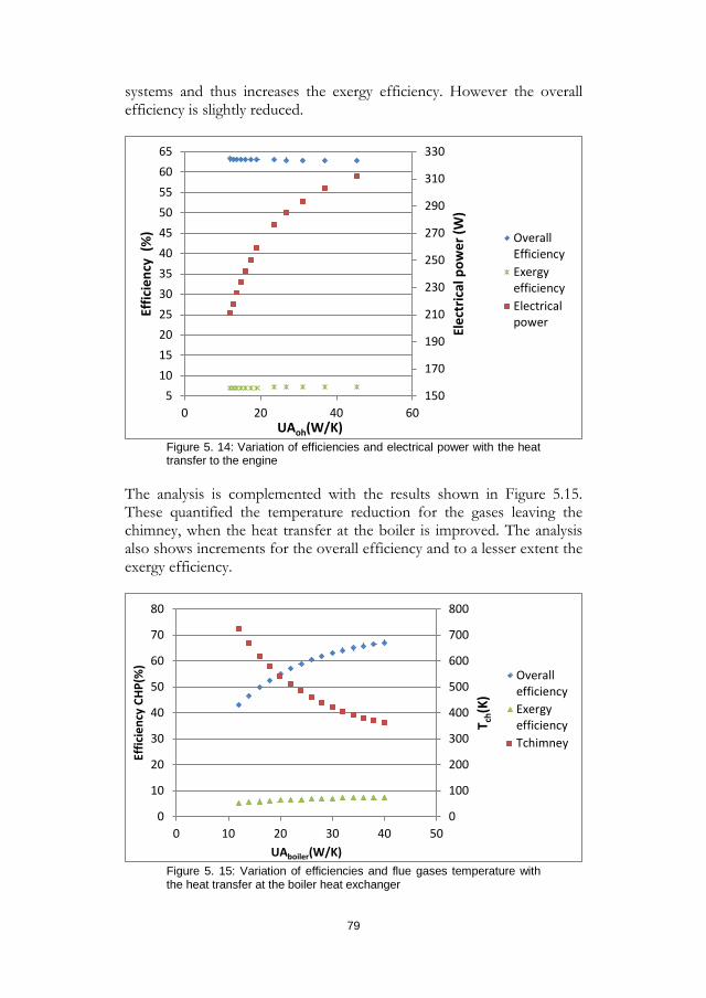
systems and thus increases the exergy efficiency. However the overall efficiency is slightly reduced.

Figure 5. 14: Variation of efficiencies and electrical power with the heat transfer to the engine

The analysis is complemented with the results shown in Figure 5.15. These quantified the temperature reduction for the gases leaving the chimney, when the heat transfer at the boiler is improved. The analysis also shows increments for the overall efficiency and to a lesser extent the exergy efficiency.

Figure 5. 15: Variation of efficiencies and flue gases temperature with the heat transfer at the boiler heat exchanger

150

170

190

210

230

250

270

290

310

330

5101520253035404550556065

0 20 40 60

Elec

tric

al p

ower

(W)

Effic

ienc

y (%

)

UAoh(W/K)

OverallEfficiencyExergyefficiencyElectricalpower

0

100

200

300

400

500

600

700

800

0

10

20

30

40

50

60

70

80

0 10 20 30 40 50

T ch(

K)

Effic

ienc

y CH

P(%

)

UAboiler(W/K)

OverallefficiencyExergyefficiencyTchimney

79

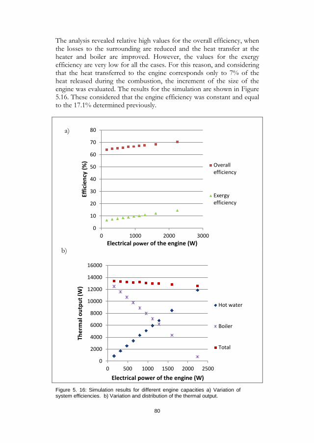
The analysis revealed relative high values for the overall efficiency, when the losses to the surrounding are reduced and the heat transfer at the heater and boiler are improved. However, the values for the exergy efficiency are very low for all the cases. For this reason, and considering that the heat transferred to the engine corresponds only to 7% of the heat released during the combustion, the increment of the size of the engine was evaluated. The results for the simulation are shown in Figure 5.16. These considered that the engine efficiency was constant and equal to the 17.1% determined previously.

Figure 5. 16: Simulation results for different engine capacities a) Variation of system efficiencies. b) Variation and distribution of the thermal output.

0

10

20

30

40

50

60

70

80

0 1000 2000 3000

Effic

ienc

y (%

)

Electrical power of the engine (W)

Overallefficiency

Exergyefficiency

0

2000

4000

6000

8000

10000

12000

14000

16000

0 500 1000 1500 2000 2500

Ther

mal

out

put (

W)

Electrical power of the engine (W)

Hot water

Boiler

Total

a)

b)

80

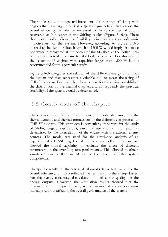
The results show the expected increment of the exergy efficiency with engines that have larger electrical outputs (Figure 5.16.a). In addition, the overall efficiency will also be increased thanks to the thermal output recovered as hot water at the Stirling cooler (Figure 5.16.b). These theoretical results indicate the feasibility to increase the thermodynamic attractiveness of the system. However, according to Figure 5.16.b increasing the size to values larger than 1200 W would imply that more hot water is recovered at the cooler of the SE than at the boiler. This represents practical problems for the boiler operation. For this reason the selection of engines with capacities larger than 1200 W is not recommended for this particular study.

Figure 5.16.b integrates the relation of the different energy outputs of the system and thus represents a valuable tool to assess the sizing of CHP-SE systems. For example, when the size for the engine is stablished the distribution of the thermal outputs, and consequently the practical feasibility of the system would be determined.


The chapter presented the development of a model that integrates the thermodynamic and thermal interactions of the different components of CHP-SE systems. This approach is particularly important for the study of Stirling engine applications, since the operation of the system is determined by the interrelation of the engine with the external energy sources. The model was used for the simulation analysis of an experimental CHP-SE rig fuelled on biomass pellets. The analysis showed the model capability to evaluate the effect of different parameters on the overall system performance. This allowed to obtain simulation curves that would assess the design of the system components.

The specific results for the case study showed relative high values for the overall efficiency, but also reflected the sensitivity to the energy losses. For the exergy efficiency, the values indicated a low quality for the energy outputs. However, the simulation results showed that the increment of the engine capacity would improve this thermodynamic indicator without affecting the overall performance of the system.

81

6 Concluding Remarks

Stirling engine systems have evolved from the first engine used to drive a quarry water pump to some advanced engine prototypes that can be used for space exploration. These developments have been mainly driven by experimental trial and error tests that guided to the construction of few successful prototypes, and thus resulted into a very expensive and discouraging technology. This reflects the importance of theoretical studies that could permit to understand and explain the operating principles of these systems.

The present work used this theoretical approach for the design improvement of Stirling engine systems and also to evaluate their integration into micro CHP systems.

The first part of the study presented the development and validation of a model that integrated the thermodynamic, heat transfer and mechanical interactions that govern the engine operation. The integration of these concepts required a slightly complex numerical solution, but allowed to identify important relations between different design and operating parameters. These relations included:

• The need to account for the equilibrium between the external heat transferred to the engine and the heat required to complete the thermodynamic cycle.

• The relevance that the forced work have for the adequate determination of the operational parameters of reciprocating engines

• The design of a cranck mechanism that would permit a good balance for the movements of the piston and displacer of the engine, and thus could reduce the forced expansion and compression processes.

• The need to design heat exchangers that would balance the effects of the dead volumes and the required heat transfer areas

• The presence of two conflictive design objectives: the design towards increased power outputs, and the design towards engines with higher efficiencies

The model presented additional results that allowed a deeper insight of the engine operation. These include: the temperature and mass flow distribution along the engine; the calculation of the cyclic expansion and compression work; the pressure drop and heat flow through the heat exchangers; conductive, shuttle and regenerator thermal losses; and the power output and efficiency of the engine.

82

The mentioned results probed the capability of the model to address the first research objective, since represent a valuable tool to assess the design improvements of Stirling prototypes.

The second part of the study extended the analysis towards the integration of the engine into micro CHP systems. The models developed for this section considered the need to reflect the thermal and thermodynamic interactions of the different components at micro scale sizes. This approach allowed to identify the effect that each component has on the overall system performance. Therefore, the results allowed to respond to the second objective of the research: The proposal of design guidelines that would increase the thermodynamic performance of the overall system.

In general, the research showed the relevance that the theoretical analysis supported by numerical computations have on the development of alternative energy technologies, such as the Stirling engine technology. The use of these methodologies complement experimental studies, reduce the costs related to the development of prototypes, and would permit to improve the innovation on the design. Therefore, would accelerate the integration of new competitive technologies in the energy sector.

6 . 1 F u t u r e w o r k

Stirling engine model development

• The correlations for the heat transfer and pressure drops were based in general studies reported in the literature. These could be improved by determining experimental correlations for the particular prototype. The update of the correlations could be easily implemented thanks to the flexible structure of the model.

• It is important to obtain additional experimental data that could validate the energy losses calculated with the model. Particularly the pressure drops at the regenerator and the mechanical efficiency of the system.

• The model developed could be implemented in an open source platform and thus spread its use.

• The engine spaces could be discretized into more control volumes. The advantages and disadvantages of this discretization could be compared with the present results.

• Cost modules could be included and thus extend the analysis towards the development of low cost prototypes.

83

• CFD computations are another approach that could be explored depending of the objectives that the model should response.

Parametric analysis of the engine

• An optimization methodology could be used to extend the sensitivity analysis. Multi-objective optimization could be important to evaluate the conflicting objectives identified.

• The study could be extended to the analysis of free piston engines.

Analysis of the SE-CHP system

• CFD analysis could be used to study the heat transfer process in the combustion chamber. This will provide more insights for the temperature distribution around the external heat exchanger of the engine and thus guide better the design.

• The steady state model could be extended to a dynamic model. This will allow studying the performance of the system under different energy loads and then implementing different control strategies.

• Techno-economic analysis for the systems are required to complement the results of the present study

84

7 References

[1] Internaltional Energy Agency, “The future and our energy sources - ETP 2014 report,” 2014.

[2] R. D. Vidic, S. L. Brantley, J. M. Vandenbossche, D. Yoxtheimer, and J. D. Abad, “Impact of shale gas development on regional water quality.,” Science (New York, N.Y.), vol. 340, no. 6134, p. 1235009, May 2013.

[3] Colombo, Emanuela, S. Bologna, and D. Masera, Renewable energy for unleashing sustainable development Ebook. 2013.

[4] N. El Bassam, “Renewable energy for rural communities,” Renewable Energy, vol. 24, pp. 401–408, 2001.

[5] S. Chu and A. Majumdar, “Opportunities and challenges for a sustainable energy future.,” Nature, vol. 488, no. 7411, pp. 294–303, Aug. 2012.

[6] L. Dong, H. Liu, and S. Riffat, “Development of small-scale and micro-scale biomass-fuelled CHP systems – A literature review,” Applied Thermal Engineering, vol. 29, no. 11–12, pp. 2119–2126, Aug. 2009.

[7] H. I. Onovwiona and V. I. Ugursal, “Residential cogeneration systems: review of the current technology,” Renewable and Sustainable Energy Reviews, vol. 10, no. 5, pp. 389–431, Oct. 2006.

[8] J. A. Araoz, “Micro polygeneration systems and its potential in Bolivia,” Stockholm, 2015.

[9] D. G. Thombare and S. K. Verma, “Technological development in the Stirling cycle engines,” Renewable and Sustainable Energy Reviews, vol. 12, no. 1, pp. 1–38, Jan. 2008.

[10] Y. C. Hsieh, T. C. Hsu, and J. S. Chiou, “Integration of a free-piston Stirling engine and a moving grate incinerator,” Renewable Energy, vol. 33, no. 1, pp. 48–54, Jan. 2008.

[11] B. Thomas, “Benchmark testing of Micro-CHP units,” Applied Thermal Engineering, vol. 28, no. 16, pp. 2049–2054, Nov. 2008.

[12] B. Kongtragool and S. Wongwises, “Investigation on power output of the gamma-configuration low temperature differential Stirling engines,” Renewable Energy, vol. 30, no. 3, pp. 465–476, Mar. 2005.

[13] B. Aoun, S. Thiers, and B. Peuportier, “Experimental Characterization of a Micro-CHP unit based on a Stirling Engine, fueled by Wood Pellets,” … International Stirling Engine …, 2009.

[14] A. J. Organ, Stirling Cycle Engines: Inner Workings and Design. John Wiley & Sons, 2013.

[15] J. M. Strauss and R. T. Dobson, “Evaluation of a second order simulation for Sterling engine design and optimisation,” Energy in Southern Africa, vol. 21, no. 2, pp. 17–29, 2010.

[16] H. Snyman, “Second Order Analyses Methods for Stirling Engine Design,” Stellenbosch: University of Stellenbosch, 2007.

[17] I. Urieli and D. M. Berchowitz, Stirling cycle engine analysis. Bristol: Hilger Ltd., 1984.

85

[18] A. J. Organ, Thermodynamics and Gas Dynamics of the Stirling Cycle Machine. Cambridge University Press, 1992.

[19] R. W. Dyson, S. D. Wilson, and R. C. Tew, “Review of Computational Stirling Analysis Methods,” no. October, 2004.

[20] R. C. Tew, Initial comparison of single cylinder Stirling engine computer model predictions with test results (DOE/NASA/1040-78/30). for sale by the National Technical Information Service, 1979.

[21] Genoastirling S.r.l., “www.genoastirling.com,” 2014. [Online]. Available: http://www.genoastirling.com/. [Accessed: 12-Mar-2014].

[22] R. C. . J. Tew, L. G. Thieme, and D. Miao, “Initial comparison of single cylinder Stirling engine computer model predictions with test results,” Feb. 1979.

[23] E. Cardozo, C. Erlich, A. Malmquist, and L. Alejo, “Integration of a wood pellet burner and a Stirling engine to produce residential heat and power,” Applied Thermal Engineering, Aug. 2014.

[24] G. Walker and J. R. Senft, Free Piston Stirling Engines, vol. 12. Berlin, Heidelberg: Springer Berlin Heidelberg, 1985.

[25] R. Stirling, “Stirling patent of 1816/1817,” in The Philips Stirling engine, Amsterdam, The Netherlands: Elsevier Science Publishers B.V., 1991, p. Appendix B.

[26] S. Carnot, Reflections on the Motive Power of Fire: And Other Papers on the Second Law of Thermodynamics, Illustrate. New York: Dover Publications, 2005.

[27] The Air Engine: Stirling Cycle Power for a Sustainable Future [Hardcover]. CRC Press, 2007, p. 276.

[28] J. STIRLING, “DESCRIPTION OF STIRLING’S IMPROVED AIR ENGINE. (INCLUDES PLATE).,” Minutes of the Proceedings, vol. 4, no. 1845, pp. 348–355, Jan. 1845.

[29] J. SMITH, J. JEFFREYS, G. COTTAM, J. STIRLING, J. FIELD, A. GORDON, J. LESLIE, J. WALKER, R. STEPHENSON, S. G. CAYLEY, and S. C. HOMERSHAM, “DISCUSSION. STIRLING’S IMPROVED AIR ENGINE.,” Minutes of the Proceedings, vol. 4, no. 1845, pp. 355–361, Jan. 1845.

[30] C. M. Hargreaves, “The hot-air engine,” in The Philips Stirling engine, Amsterdam, The Netherlands: Elsevier Science Publishers B.V., 1991, pp. 1–25.

[31] A. Ross, Stirling Cycle Engines. Solar Engines, 1981.

[32] J. Senft and J. R. Senft, An Introduction to Stirling Engines. Moriya Pr, 1993, p. 80. [33] C. M. Hargreaves, “The twentienth century revival,” in The Philips Stirling engine,

Amsterdam, The Netherlands: Elsevier Science Publishers B.V., 1991, pp. 27–81.

[34] C. M. Hargreaves, The Philips Stirling engine. Amsterdam, The Netherlands: Elsevier Science Publishers B.V., 1991, pp. 9–10.

[35] C. M. Hargreaves, “The past and the future,” in The Philips Stirling engine, Amsterdam, The Netherlands: Elsevier Science Publishers B.V., 1991, pp. 403–418.

[36] K. Sato, N. Ohiwa, A. Ishikawa, H. Shimojima, A. Nishiyama, and Y. Moriya, “Development of Small-Scale CHP Plant with a Wood Powder-Fueled Stirling Engine,” Journal of Power and Energy Systems, vol. 2, no. 5, pp. 1221–1231, 2008.

[37] a Nishiyama, H. Shimojima, a Ishikawa, Y. Itaya, S. Kambara, H. Moritomi, and S. Mori, “Fuel and emissions properties of Stirling engine operated with wood powder,” Fuel, vol. 86, no. 15, pp. 2333–2342, Oct. 2007.

86

[38] F. Biedermann, H. Carlsen, M. Schöch, and I. Obernberger, “Operating experiences with a small-scale chp pilot plant based on a 35 kw el hermetic four cylinder stirling engine for biomass fuels,” 2004.

[39] M. Pålsson and H. Carlsen, “Development of a wood powder fuelled 35 kW Stirling CHP unit,” Proceedings of the 11th ISEC (International Stirling Engine Conference), pp. 221 – 230, 2003.

[40] M. Zeiler, R. Padinger, J. Spitzer, and E. Podesser, “Operating experiences with biomass driven Stirling engines ; 3 kW and 30 kW,” vol. c, pp. 5–7.

[41] V. S. Reddy, “Exergetic analysis and performance evaluation of parabolic dish Stirling engine solar power plant,” International Journal of energy research, no. May 2012, pp. 1287–1301, 2013.

[42] G. Walker, Stirling-cycle Engines. Oxford: Clarendon Press, 1973.

[43] I. Urieli, “Stirling Cycle Machine Analysis,” 2014. [Online]. Available: http://www.ohio.edu/mechanical/stirling/engines/engines.html.

[44] F. P. Incropera, A. S. Lavine, and D. P. DeWitt, Fundamentals of Heat and Mass Transfer. John Wiley & Sons, 2011, p. 1048.

[45] W. M. Kays and A. L. London, Compact heat exchangers. Krieger Pub. Co., 1984.

[46] M. Kuosa, K. Saari, a. Kankkunen, and T.-M. Tveit, “Oscillating flow in a stirling engine heat exchanger,” Applied Thermal Engineering, vol. 45–46, pp. 15–23, Dec. 2012.

[47] B. Thomas and D. Pittman, “AIAA-2000-2812 UPDATE ON THE EVALUATION OF DIFFERENT CORRELATIONS FOR THE FLOW FRICTION FACTOR AND HEAT TRANSFER OF STIRLING ElNGINE REGENERATORS,” pp. 76–84, 2000.

[48] R. Bowman, F. Ritzert, and M. Freedman, “Evaluation of Candidate Materials for a High-Temperature Stirling Convertor Heater Head,” Dec. 2003.

[49] L. G. Thieme and J. G. Schreiber, “Advanced Technology Development for Stirling Convertors,” Sep. 2004.

[50] M. Kuosa, J. Kaikko, and L. Koskelainen, “The impact of heat exchanger fouling on the optimum operation and maintenance of the Stirling engine,” Applied Thermal Engineering, vol. 27, no. 10, pp. 1671–1676, Jul. 2007.

[51] D. Isaac, “Fluid heat exchanger,” US200220084065 A104-Jul-2002.

[52] J. Donald Isaac, “Stirling engine with high pressure fluid heat exchanger,” US6715285 B206-Apr-2004.

[53] D. A. CLARK and J. R. LOWRIE, “HEAT TRANSFER HEAD FOR A STIRLING ENGINE.” 22-Feb-2002.

[54] M. Kanzaka and M. Iwabuchi, “Study on heat transfer of heat exchangers in the Stirling engine - Performance of heat exchangers in the test Stirling engine,” JSME International Journal, vol. 35, pp. 647–652, 1992.

[55] F. de Monte, “Thermal Analysis of the Heat Exchangers and Regenerator in Stirling Cycle Machines,” Journal of Propulsion and Power, vol. 13, no. 3, pp. 404–411, May 1997.

[56] J. Škorpík, “Stirlingův motor-english version,” Transformační technologie. [Online]. Available: http://www.transformacni-technologie.cz/en_stirlinguv-motor.html. [Accessed: 19-Nov-2014].

[57] G. Walker and J. R. Senft, Free Piston Stirling Engines, vol. 12. Berlin, Heidelberg: Springer Berlin Heidelberg, 1985.

87

[58] A. R. Tavakolpour, A. Zomorodian, and A. Akbar Golneshan, “Simulation, construction and testing of a two-cylinder solar Stirling engine powered by a flat-plate solar collector without regenerator,” Renewable Energy, vol. 33, no. 1, pp. 77–87, Jan. 2008.

[59] A. J. Organ, “Proceedings of the Institution of Mechanical Engineers, Part C: Journal of Mechanical Engineering Science,” 1987.

[60] M. B. Ibrahim, R. C. Tew, and Jr., Stirling Convertor Regenerators, vol. 16. CRC Press, 2011, p. 487.

[61] J. G. Wood, “Advanced Stirling Convertor Update,” in AIP Conference Proceedings, 2006, vol. 813, pp. 640–652.

[62] M. B. Ibrahim, D. Gedeon, G. Wood, and J. McLean, “A Microfabricated Segmented-Involute-Foil Regenerator for Enhancing Reliability and Performance of Stirling Engines. Phase III Final Report for the Radioisotope Power Conversion Technology NRA,” 2009.

[63] R. Tew, M. Ibrahim, D. Danila, T. Simon, S. Mantell, L. Sun, D. Gedeon, K. Kelly, J. Mclean, G. Wood, and S. Qiu, “A Microfabricated Involute-Foil Regenerator for Stirling Engines October 2007,” no. October, 2007.

[64] T. Takeuchi, D. Kitahama, A. Matuguchi, N. Kagawa, and S. Tsuruno, “Performance of New Mesh Sheet for Stirling Engine Regenerater,” in 2nd International Energy Conversion Engineering Conference, 2004.

[65] D. Kitahama, H. Takizawa, N. Kagawa, A. Matsuguchi, and S. Tsuruno, “Performance of New Mesh Sheet For Stirling Engine Regenerator,” 2003.

[66] H. Takizawa, N. Kagawa, A. Matsuguchi, and S. Tsuruno, “Performance of new matrix for Stirling engine regenerator,” in IECEC ’02. 2002 37th Intersociety Energy Conversion Engineering Conference, 2002., 2002, pp. 491–496.

[67] T. Knowles, “Composite matrix regenerator for Stirling engines, National Aeronautics Space Administration,” 1997.

[68] Stirling-Power, “Stirling Power.” [Online]. Available: http://www.sp-usa.com/. [Accessed: 23-Nov-2014].

[69] M. A.Ross, “Balanced crankshaft mechanism for the two piston Stirling engine.” U.S. Patent No. 4,138,897, Washington, 13-Feb-1979.

[70] W. T. Beale, “Self-starting, free piston Stirling engine,” US4036018 A19-Jul-1977.

[71] S. Wilson, R. Dyson, R. Tew, and M. Ibrahim, “Multi-D CFD Modeling of a Free-Piston Stirling Convertor at NASA GRC,” arc.aiaa.org.

[72] S.-Y. Kim and D. M. Berchowitz, “Specific Power Estimations for Free-Piston Stirling Engines,” in 4th International Energy Conversion Engineering Conference and Exhibit, San Diego, 2006, pp. 1–8.

[73] S. OBARA, I. TANNO, S. KITO, A. HOSHI, and S. SASAKI, “Exergy analysis of the woody biomass Stirling engine and PEM-FC combined system with exhaust heat reforming,” International Journal of Hydrogen Energy, vol. 33, no. 9, pp. 2289–2299, May 2008.

[74] A. Smith, G. Lee, and W. Newman, “Analysis of hybrid fuel-cell/stirling-engine systems for domestic combined heat and power,” in 2012 IEEE Energytech, 2012, pp. 1–7.

[75] J. J. Klemeš, S. Pierucci, V. Kuhn, J. Klemeš, and I. Bulatov, “MicroCHP: Overview of selected technologies, products and field test results,” Applied Thermal Engineering, vol. 28, no. 16, pp. 2039–2048, 2008.

88

[76] S. Obara, S. Kito, A. Hoshi, and S. Sasaki, “Study on woody biomass Stirling cycle for cold region houses,” no. August 2007, pp. 152–163, 2009.

[77] ProEcopolyNet, “Experimental Examination of different micro-CHP’s - Best practice Sheet - Germany (en).” [Online]. Available: http://www.buildup.eu/cases/19113. [Accessed: 19-Aug-2014].

[78] A. NISHIYAMA, H. SHIMOJIMA, A. ISHIKAWA, Y. ITAYA, S. KAMBARA, H. MORITOMI, and S. MORI, “Fuel and emissions properties of Stirling engine operated with wood powder,” Fuel, vol. 86, no. 15, pp. 2333–2342, Oct. 2007.

[79] http://www.entercomunicacion.com, “Whispergen-Europe - The Stirling Engine.” [Online]. Available: http://www.whispergen-europe.com/stirling_en.php. [Accessed: 20-Nov-2014].

[80] E. P. for E. E. in Buildings, “SOLO Stirling 161 - Fact Sheet - Germany (en).” [Online]. Available: http://www.buildup.eu/cases/19164. [Accessed: 20-Nov-2014].

[81] Sunpower, “Sunpower Inc. - Welcome.” [Online]. Available: http://sunpowerinc.com/welcome/. [Accessed: 20-Nov-2014].

[82] Qnergy, “Qnergy.” [Online]. Available: http://www.qnergy.com/. [Accessed: 20-Nov-2014].

[83] Cleanergy, “Cleanergy - A new generation of sustainable energy.” [Online]. Available: http://cleanergy.com/. [Accessed: 20-Nov-2014].

[84] Wudag, “Company | Stirling Energie WUDAG Dezentrale Energiesysteme.” [Online]. Available: http://www.stirling-energie.de/en/company. [Accessed: 20-Nov-2014].

[85] M. E. Corria, V. M. Cobas, and E. Silva Lora, “Perspectives of Stirling engines use for distributed generation in Brazil,” Energy Policy, vol. 34, no. 18, pp. 3402–3408, Dec. 2006.

[86] J. R. Senft, “A simple derivation of the generalized Beale number,” IECEC ’82; Proceedings of the Seventeenth Intersociety Energy Conversion Engineering Conference, vol. -1, pp. 1652–1655, 1982.

[87] R. Dyson, S. Wilson, and R. Tew, “Review of Computational Stirling Analysis Methods,” in 2nd International Energy Conversion Engineering Conference, American Institute of Aeronautics and Astronautics, 2004.

[88] R. Dyson, S. Wilson, and R. Tew, “Review of Computational Stirling Analysis Methods,” in 2nd International Energy Conversion Engineering Conference, American Institute of Aeronautics and Astronautics, 2004.

[89] F. Formosa, “Coupled thermodynamic–dynamic semi-analytical model of free piston Stirling engines,” Energy Conversion and Management, vol. 52, no. 5, pp. 2098–2109, May 2011.

[90] C.-H. Cheng and Y.-J. Yu, “Numerical model for predicting thermodynamic cycle and thermal efficiency of a beta-type Stirling engine with rhombic-drive mechanism,” Renewable Energy, vol. 35, no. 11, pp. 2590–2601, Nov. 2010.

[91] N. Seraj Mehdizadeh and P. Stouffs, “Simulation of a Martini Displacer Free Piston Stirling Engine for Electric Power Generation,” International Journal of Thermodynamics, vol. 3, no. 1. pp. 27–34.

[92] N. Parlak, A. Wagner, M. Elsner, and H. S. Soyhan, “Thermodynamic analysis of a gamma type Stirling engine in non-ideal adiabatic conditions,” Renewable Energy, vol. 34, no. 1, pp. 266–273, Jan. 2009.

89

[93] T. Finkelstein, “Computer analysis of Stirling engines,” Adv. Cryog. Eng.; (United States), vol. 20, Jan. 1975.

[94] I. Urieli, C. J. Rallis, and D. M. Berchowitz, “Computer simulation of Stirling cycle machines,” 12th Intersociety Energy Conversion Engineering Conference, vol. -1, pp. 1512–1521, 1977.

[95] A. Schock, “Nodal analysis of Stirling cycle devices,” In: Intersociety Energy Conversion Engineering Conference, vol. 3, pp. 1771–1779, 1978.

[96] D. Gedeon, “Sage - Object-oriented software for Stirling machine design,” in Intersociety Energy Conversion Engineering Conference, American Institute of Aeronautics and Astronautics, 1994.

[97] R. C. Tew, K. Jefferies, D. Miao, U. S. D. of E. D. of T. E. Conservation, and L. R. Center, A Stirling Engine Computer Model for Performance Calculations (Google eBook). Department of Energy, Office of Conservation and Solar Applications, Division of Transportation Energy Conservation, 1978, p. 100.

[98] A. J. Organ, “Gas dynamics of the temperature-determined Stirling cycle,” ARCHIVE: Journal of Mechanical Engineering Science 1959-1982 (vols 1-23), vol. 23, no. 4, pp. 207–216, Aug. 1981.

[99] V. H. Larson, “Characteristic dynamic energy equations for Stirling cycle analysis,” Proc., Intersoc. Energy Convers. Eng. Conf.; (United States), vol. 2, Aug. 1981.

[100] K. Mahkamov and D. Djumanov, “Three-dimensional CFD modeling of a Stirling engine,” Proceedings of the 11th International Stirling engine conference, vol. Vol. 19, 2003.

[101] M. Ibrahim, R. Tew, Z. Zhang, D. Gedeon, and T. Simon, “CFD Modeling of Free-Piston Stirling Engines,” Cleveland, Ohio, 2001.

[102] K. Alanne, N. Söderholm, K. Sirén, and I. Beausoleil-Morrison, “Techno-economic assessment and optimization of Stirling engine micro-cogeneration systems in residential buildings,” Energy Conversion and Management, vol. 51, no. 12, pp. 2635–2646, 2010.

[103] K. Lombardi, V. I. Ugursal, and I. Beausoleil-Morrison, “Proposed improvements to a model for characterizing the electrical and thermal energy performance of Stirling engine micro-cogeneration devices based upon experimental observations,” Applied Energy, vol. 87, no. 10, pp. 3271–3282, Oct. 2010.

[104] H. Ribberink, D. Bourgeois, and I. Beausoleil-Morrison, “A plausible forecast of the energy and emissions performance of mature-technology Stirling engine residential cogeneration systems in Canada,” Journal of Building Performance Simulation, vol. 2, no. 1, pp. 47–61, Mar. 2009.

[105] V. Dorer and A. Weber, “Energy and carbon emission footprint of micro-CHP systems in residential buildings of different energy demand levels,” Journal of Building Performance Simulation, vol. 2, no. 1, pp. 31–46, Mar. 2009.

[106] F. Miccio, “On the integration between fluidized bed and Stirling engine for micro-generation,” Applied Thermal Engineering, vol. 52, no. 1, pp. 46–53, 2013.

[107] K. Hirata, “Schmidt theory for Stirling engines,” Stirling Engine home page. Disponível em, 1997.

[108] W. R. Martini, “STIRLING ENGINE DESIGN MANUAL,” 1978.

[109] B. Thomas and D. Pittman, “Update on the evaluation of different correlations for the flow friction factor and heat transfer of Stirling engine regenerators,” in

90

Collection of Technical Papers. 35th Intersociety Energy Conversion Engineering Conference and Exhibit (IECEC) (Cat. No.00CH37022), 2000, vol. 1, pp. 76–84.

[110] D. Gedeon and J. Wood, “Oscillating-flow regenerator test rig: Woven screen and metal felt results,” NASA STI/Recon Technical Report N, 1992.

[111] Y. Timoumi, I. Tlili, and S. Ben Nasrallah, “Design and performance optimization of GPU-3 Stirling engines,” Energy, vol. 33, no. 7, pp. 1100–1114, Jul. 2008.

[112] J. R. Senft, Mechanical Efficiency of Heat Engines. Cambridge University Press, 2007.

[113] G. Sewell, Numerical Solution of Ordinary and Partial Differential Equations (2nd Edition). John Wiley & Sons, 2005.

[114] D. D. Do Richard G. Rice, Applied Mathematics And Modeling For Chemical Engineers [Hardcover]. Wiley-AIChE; 2 edition, 2012, p. 400.

[115] R. C. Tew, L. G. Thieme, and D. Miao, Initial Comparison of Single Cylinder Stirling Engine Computer Model Predictions with Test Results. The Division, 1979, p. 19.

[116] L. G. Thieme, U. S. D. of Energy. Division of Transportation Energy Conservation, and L. R. Center, Low-power Baseline Test Results for the GPU 3 Stirling Engine. The Division, 1979.

[117] R. C. Tew, K. Jefferies, D. Miao, U. S. D. of E. D. of T. E. Conservation, and L. R. Center, A Stirling Engine Computer Model for Performance Calculations (Google eBook). Department of Energy, Office of Conservation and Solar Applications, Division of Transportation Energy Conservation, 1978, p. 100.

[118] R. Gheith, F. Aloui, and S. Ben Nasrallah, “Study of the regenerator constituting material influence on a gamma type Stirling engine,” Journal of Mechanical Science and Technology, vol. 26, no. 4, pp. 1251–1255, Apr. 2012.

[119] H. Thunman, “Principles and Models of Solid Fuel Combustion,” 2001.

[120] T. Klason, “Modelling of Biomass Combustion in Furnaces Phd Thesis,” Lund Institute of Technology, 2006.

[121] X. Zhang, “Numerical modeling of biomass combustion in a stoker boiler, Phd Thesis,” 2011.

[122] R. Bauer, M. Gölles, T. Brunner, N. Dourdoumas, and I. Obernberger, “Modelling of grate combustion in a medium scale biomass furnace for control purposes,” Biomass and Bioenergy, vol. 34, pp. 417–427, 2010.

[123] R. Scharler, C. Benesch, K. Schulze, and I. Obernberger, “CFD Simulations As Efficient Tool For The Development and Optimisation of Small-Scale Biomass Furnaces and Stoves,” in 19th European Biomass Conference and Exhibition, 2011, no. x.

[124] M. Y. Haller†, J. Paavilainen, L. Konersmann, R. Haberl, A. Dröscher, E. Frank, C. Bales, and W. Streicher, “A unified model for the simulation of oil, gas and biomass space heating boilers for energy estimating purposes. Part I: Model development,” Journal of Building Performance Simulation, vol. 4, no. 1, pp. 1–18, Jul. 2010.

[125] B. J. McBride, S. Gordon, and M. A. Reno, “Coefficientes for Calculating Thermodynamic and Transport Properties of Individual Species, National Aeronautics and Space Administration,” 1993.

[126] E. Cardozo, C. Erlich, L. Alejo, and T. H. Fransson, “Combustion of agricultural residues: An experimental study for small-scale applications,” Fuel, vol. 115, pp. 778–787, Jan. 2014.

91

Documents

Thermodynamic analysis of Stirling engine systems798500/FULLTEXT01.pdf · plants based on Stirling Engines (SE) have attracted the interest among research and industry due to the