Thermo Scientific AutoCONFIG Software Startup Guide

Part of Thermo Fisher Scientific

AutoCONFIG™ Software for AutoEXEC & AutoPILOT PRO Systems Startup GuideP/N 1-0485-068

Revision D

AutoCONFIG™ Software for AutoEXEC & AutoPILOT PRO Systems Startup GuideP/N 1-0485-068

Revision D

© 2011 Thermo Fisher Scientific Inc. All rights reserved.

“Microsoft” and “Windows” are either registered trademarks or trademarks of Microsoft Corporation in the United States and/or other countries.

All other trademarks are the property of Thermo Fisher Scientific Inc. and its subsidiaries.

Thermo Fisher Scientific Inc. (Thermo Fisher) makes every effort to ensure the accuracy and completeness of this manual. However, we cannot be responsible for errors, omissions, or any loss of data as the result of errors or omissions. Thermo Fisher reserves the right to make changes to the manual or improvements to the product at any time without notice.

The material in this manual is proprietary and cannot be reproduced in any form without expressed written consent from Thermo Fisher.

This page intentionally left blank.

Thermo Fisher Scientific AutoCONFIG Software Startup Guide v

Revision History

Revision Level Date Comments

A 09-2009 Initial release (ERO 7100).

B 06-2010 Revised per ECO 7324.

C 02-2011 Revised per ECO 7641.

D 07-2011 Revised per ECO 7763.


Contents Chapter 1 General Information ......................................................................................... 1-1

About this Guide................................................................................. 1-1 Receiving the Instrument .................................................................... 1-1

Chapter 2 Installation & Connections ............................................................................. 2-1 Hardware ............................................................................................ 2-1 Communication Connections for AutoEXEC Flow Computer ........... 2-1 Communication Connections for AutoPILOT PRO Flow Computer. 2-3 Software Installation............................................................................ 2-3

Establishing Communications........................................................................ 3-1 Chapter 3 Setting Communication Parameters .................................................... 3-1

Creating an Off Line Connection..................................................... 3-2 Creating a Remote Connection via TCP/IP ..................................... 3-4 Creating a Local Connection............................................................ 3-5

Setting up an IP Address ..................................................................... 3-8 Adding Entries to an Existing Configuration..................................... 3-12

Special Notes when Adding Physical Input Entries......................... 3-19 Special PC Setup for AutoCONFIG Software................................... 3-24

Configuring a Meter Run with the Measurement Config Wizard............ 4-1 Chapter 4 Overview............................................................................................. 4-1 For Gas Meter Runs............................................................................ 4-2 For Liquid Flow Runs ....................................................................... 4-10

Chapter 5 Gas Quality ......................................................................................................... 5-1 Configuring a Gas Chromatograph ..................................................... 5-1 Gas Quality without a GC .................................................................. 5-3

Chapter 6 System Status & System Control Tables ...................................................... 6-1 System Status (Table #30)................................................................... 6-1 System Control (Table #31)................................................................ 6-4

Chapter 7 AutoCONFIG Software & the Help System................................................... 7-1 Using the Software .............................................................................. 7-1 Using the Help System........................................................................ 7-1 Page Level Help .................................................................................. 7-3 Printing the Help System .................................................................... 7-3

Thermo Fisher Scientific AutoCONFIG Software Startup Guide vii

Contents

viii AutoCONFIG Software Startup Guide Thermo Fisher Scientific

Glossary............................................................................................ GLOSSARY-1

Index .......................................................................................................... INDEX-1

Chapter 1

General Information

About this Guide This document is a startup guide for the Thermo Scientific AutoCONFIG software when used with the Thermo Scientific AutoEXEC or AutoPILOT PRO flow computers. Reading this guide will help you:

● Install the software

● Establish communications with the flow computer

● Use the Measurement Config wizard to configure meter runs

● Understand how to use the AutoCONFIG software help system, which provides details on how to use all the functions the software offers, access to other manuals, information on instrument hardware and connections, and more.

The startup guide does not provide instrument installation or specific instructions on all the software’s capabilities. For that information, refer to the instrument’s manual(s) and the AutoCONFIG software help system.

Receiving the Instrument

With your AutoEXEC or AutoPILOT PRO flow computer, you should receive the following items:

● The product user guide (p/n 1-0443-048 for AutoEXEC flow computer, 1-0500-005 for AutoPILOT PRO flow computer)

● The AutoCONFIG software startup guide (p/n 1-0485-068)

● Troubleshooting AutoEXEC and AutoPILOT PRO Systems (p/n 1-0443-072)

● If requested, the Thermo Scientific AutoCONFIG configuration software

If any of these items are missing, contact Thermo Fisher Scientific at 713-272-0404.

Thermo Fisher Scientific AutoCONFIG Software Startup Guide 1-1


Chapter 2

Installation & Connections

Hardware Refer to the instrument manual for flow computer installation and wiring instructions. If you have other instruments as part of your system, a Thermo Scientific AutoMITTER PRO transmitter for example, reference the manufacturer’s documentation.

Communication Connections for AutoEXEC Flow

Computer

A serial connection is used to establish initial communications with the instrument.

To connect your PC to a flow computer with rack or panel mount configuration (standard enclosure), use a straight through DE9 extension cable (p/n 5-0580-002) to provide connection to the local RS232 DCE port on the CPU board.

Figure 2–1. AutoEXEC CPU face plate (rack or panel mount): PC connection


Installation & Connections Communication Connections for AutoEXEC Flow Computer

To connect your PC to a flow computer with a pole mount configuration (NEMA 4X enclosure), use a 6-pin circular connector cable (p/n 3-0446-090) to connect to the bottom of the enclosure.

Warning Ensure the area is non-hazardous before connecting to the local RS232 port. ▲

Figure 2–2. Bottom view of AutoEXEC NEMA 4X enclosure (pole mount): PC connection

If the flow computer is connected directly to a network, you can establish communications with it after setting up its IP address, which is discussed in “Setting up an IP Address” in Chapter 3.

2-2 AutoCONFIG Software Startup Guide Thermo Fisher Scientific

Installation & Connections Communication Connections for AutoPILOT PRO Flow Computer


Communication Connections for AutoPILOT PRO Flow Computer

The AutoPILOT PRO main board provides one RS232 compatible local communication port (TB8) for calibration and configuration of the unit using a laptop and the AutoCONFIG software. Connection is made through the CHIT connector mounted in the bottom of the flow computer enclosure. Thermo Fisher manufactures optional cable assemblies for this connection. They are listed below.

Table 2–1. Cable assemblies for CHIT connector

Assembly P/N Description

3-0446-090 DB9S connecter with 15-ft cable for use with the six-position connecter

3-0446-090-B DB9S connecter with 25-ft cable for use with the six-position connecter

Figure 2–3. Bottom view of AutoPILOT PRO flow computer to show location of CHIT connector

Note If using the optional communication expansion board, refer to the AutoPILOT PRO user guide for wiring diagrams and jumpers settings. ▲

When you have made the required connections, you are ready to install the AutoCONFIG software. Create a folder on your hard drive, and copy the contents of the product CD into it. Double-click the setup.exe file and follow the instructions as they appear on the screen.

Software Installation


Chapter 3

Establishing Communications

After software installation is complete, double-click the AutoCONFIG icon on your desktop to open the program. The Communication Parameters screen is displayed that allows you to create connections and establish communications. Once communication is established, the main screen will be displayed.

Note If you establish communications and notice that the software is running slowly or you receive COMM errors, refer to “Special PC Setup for AutoCONFIG Software” at the end of this chapter. ▲

If communications do not establish, check the connections between the flow computer and the PC.

Setting Communication

Parameters

ting Communication

Parameters

The Communication Parameters screen allows you to set up connection information for multiple locations or units. There are three types of connections: off line, remote via TCP/IP, and local (RS232 serial).

Initial communication is established via a local connection. To do this, ensure the proper connections are made between the flow computer and the PC. Open the software, and go to “Creating a Local Connection” for instructions on how to establish initial communication with the flow computer via the AutoCONFIG software.

Once you have done this, return to this section for information on how to create an off line connection or a remote connection via TCP/IP. You can open the Communication Parameters screen at any time through the main menu (System > Connection) or the Connect to Unit icon on the toolbar, which is shown below.

Connect to Unit icon


Establishing Communications Setting Communication Parameters

An off line connection allows you to create or modify a configuration. Creating an Off Line Connection

Figure 3–1. Establishing an offline connection

1. Name: Enter a name that describes this connection.

2. Comm Port: Select Off Line.

3. Create a New Off Line Config?: Choose whether you want to create a default configuration or modify an existing configuration.

4. AutoEXEC/AutoPILOT PRO: Select the appropriate flow computer.

5. Adjust Table 15 Text: Checking this item allows you to edit Table #15, which is the text table.

6. Enable Calculations: Select whether you want to enable calculations for this connection.

7. Click Save and the connection will be added to the Connection List. Delete connections in the Connection List by highlighting the connection and clicking Delete.

8. To make the connection, click Connect. If you chose to create a new configuration in step 3, skip to step 10. If you chose to modify an existing configuration, continue to the next step.



9. Click the Browse button to locate the configuration file (.cfg). Open it, and it will appear in the dialog box, as shown below. Click on the file, and click Ok.

Figure 3–2. Selecting the configuration to modify

10. The New Database screen will open, which allows you to modify an existing configuration.

Caution If you are modifying an existing configuration and adding entries to a configuration item, reference “Adding Entries to an Existing Configuration” later in this chapter. If not done properly, modifying the number of entries will create an invalid configuration. ▲

Figure 3–3. New Database screen



You can establish communications with a flow computer that is connected directly to a network. Before you do this, however, you need to set up the unit’s IP address (later in this chapter). Once done, create a connection to it as described in this section.

Creating a Remote Connection via

TCP/IP

Figure 3–4. Establishing a remote connection

1. Name: Enter a name that will help you identify this connection.

2. Unit Type: Select AutoEXEC-AutoPILOT PRO.

3. Address: Enter the physical address of the unit you will connect to.

4. Comm. Port: Select TCP/IP (WINSOCK).

5. IP Address: Enter the IP address of the RTU.

6. Port: Set the port number the unit will use when communicating with the server.

7. Number of Retries: Set the number of times the software should attempt to connect to the unit before timing out and declaring failure.

8. Number of Nulls: Set the number of null bytes to pad the data packet with if there is not enough data to fill the last packet.



9. RX Delay: RX Delay is the number of seconds that the instrument should wait to receive a reply from the flow computer before it gives up and attempts another message.

10. After configuring a new connection, click Save and the connection will be added to the Connection List. When you want to make this connection, open this screen and double-click the connection in the list. Click Connect. Delete connections in the Connection List by highlighting the connection and clicking Delete. If you have problems connecting, check the hardware connections.

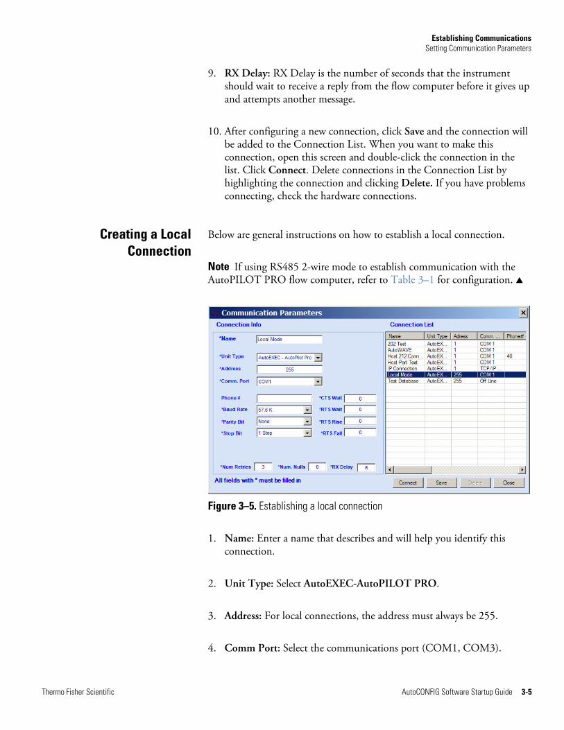
Creating a Local Connection

Below are general instructions on how to establish a local connection.

Note If using RS485 2-wire mode to establish communication with the AutoPILOT PRO flow computer, refer to Table 3–1 for configuration. ▲

Figure 3–5. Establishing a local connection

1. Name: Enter a name that describes and will help you identify this connection.

2. Unit Type: Select AutoEXEC-AutoPILOT PRO.

3. Address: For local connections, the address must always be 255.

4. Comm Port: Select the communications port (COM1, COM3).



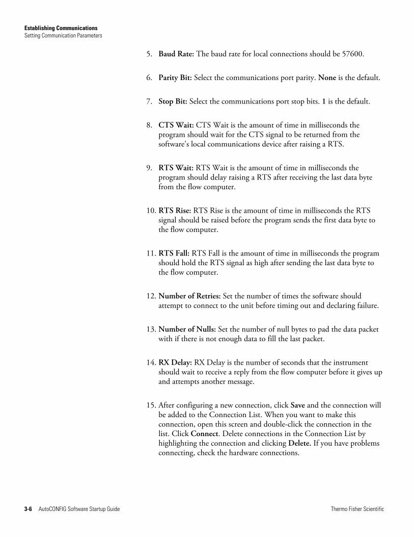
5. Baud Rate: The baud rate for local connections should be 57600.

6. Parity Bit: Select the communications port parity. None is the default.

7. Stop Bit: Select the communications port stop bits. 1 is the default.

8. CTS Wait: CTS Wait is the amount of time in milliseconds the program should wait for the CTS signal to be returned from the software's local communications device after raising a RTS.

9. RTS Wait: RTS Wait is the amount of time in milliseconds the program should delay raising a RTS after receiving the last data byte from the flow computer.

10. RTS Rise: RTS Rise is the amount of time in milliseconds the RTS signal should be raised before the program sends the first data byte to the flow computer.

11. RTS Fall: RTS Fall is the amount of time in milliseconds the program should hold the RTS signal as high after sending the last data byte to the flow computer.

12. Number of Retries: Set the number of times the software should attempt to connect to the unit before timing out and declaring failure.

13. Number of Nulls: Set the number of null bytes to pad the data packet with if there is not enough data to fill the last packet.

14. RX Delay: RX Delay is the number of seconds that the instrument should wait to receive a reply from the flow computer before it gives up and attempts another message.

15. After configuring a new connection, click Save and the connection will be added to the Connection List. When you want to make this connection, open this screen and double-click the connection in the list. Click Connect. Delete connections in the Connection List by highlighting the connection and clicking Delete. If you have problems connecting, check the hardware connections.



If using RS485 2-wire mode to establish communication with the AutoPILOT PRO flow computer, configure communication parameters based on the table below.

Table 3–1. Configuration for AutoPILOT PRO RS485 2-wire mode communication

Address Comm Port

Baud Rate

Parity Bit

CTS Wait

RTS Wait

RTS Rise

RTS Fall

Num Retries

Num Nulls

RX Delay

1 1 1200 None 0 0 0 20 3 0 5

1 1 2400 None 0 0 0 10 3 0 3

1 1 4800 None 0 0 0 5 3 0 3

1 1 9600 None 0 0 0 10 3 0 1

1 1 19.2K None 0 0 0 5 3 0 1

1 1 38.4K None 0 0 0 3 3 0 1

1 1 57.6K None 0 0 0 2 3 0 1


Establishing Communications Setting up an IP Address

Before you can establish a remote connection with a flow computer that is connected to a network, the unit’s IP address must be set up. Once this is done, you can access the flow computer from any PC that is also connected to the network.

Setting up an IP Address

1. Open the AutoCONFIG software and connect to the unit via a local connection.

2. Expand the Communications heading in the navigation bar. Select 96-Communication Port(s) > Ethernet Port #1/Ethernet Port #2 for the AutoEXEC flow computer or Ethernet Port #1 for the AutoPILOT PRO flow computer.

Figure 3–6. Setting up an IP address for a slave



3. Enable the port by changing the Calculation field to Enable. If you are setting up the port as a master, skip to step 4. If you are setting up the port as a slave, the Ethernet port will be used as the host port. The required fields are listed below in the general order of appearance on the screen.

Description: Enter a description of the port.

Mode: Select Slave.

Protocol Format: Select the slave mode protocol format (ASCII or RTU).

Address: Enter the slave mode communications address.

Write Enable: Enable/disable the port's write function.

Callout Block: This field is for future development.

Slave Password Number: You can assign up to five different passwords per communication port. This value represents the password selected to configure.

Password Register Number: The host must write the password value to the register number entered here.

Value: Enter the password value.

Defining Tasks for Ports – Comm Block Ref, Comm Block, and Block Index

You can configure up to 256 different blocks, or tasks, for each port. If you are setting up the first task for this port, select 1 in the Communications Block Reference field. If you are setting up the tenth task for this port, select 10, etc.

Next, select what type of function the port will be performing for this task in the Communications Block field. Options are: None, Modbus slave, Modbus master, chromatograph, and tank gauge.

The last step is to select the Block Index that corresponds to the communications block you chose.

Security Access: Set the access level a user must have to access this configuration from the flow computer keypad.



Comm Option block

Standard Address: This parameter defines the protocol driver’s Modbus address as an 8 bit value (0-255).

Extended Address: This parameter defines the protocol driver’s Modbus address as a 16 bit value (0-65535).

4,3,2,1 (Daniel Float), etc.: These are the options for the floating point byte order. Select how bytes and words will be sent.

Message Pad: This parameter tells the communications driver to add “nulls” (0’s) to the end of the message to assist in extending the time that RTS control is held high.

At the bottom of the screen, configure the Ethernet settings: the IP address, network mask, and Ethernet gateway. The MAC address is configured at the factory.

For Modbus using TCP/IP, enter the Modbus encapsulated port number and IP port number.

4. If you are setting up the port as a master, the Ethernet port will be used to poll another device.

Figure 3–7. Setting up an IP address for a master



Descriptor: Enter a description of the port.

Mode: Select Master.

Repeat Timer: This value controls how often the master begins a new poll. This entry is in seconds. For example, if you enter 5, the master will begin a new poll every five seconds.

Protocol Format: Select ASCII or RTU format.

Defining Tasks for Ports – Comm Block Ref, Comm Block, and Block Index

You can configure up to 256 different blocks, or tasks, for each port. If you are setting up the first task for this port, select 1 in the Communications Block Reference field. If you are setting up the tenth task for this port, select 10, etc.

Next, select what type of function the port will be performing for this task in the Communications Block field. Options are: None, Modbus slave, Modbus master, chromatograph, and tank gauge.

The last step is to select the Block Index that corresponds to the communications block you chose.

At the bottom of the screen, configure the Ethernet settings: the IP address, network mask, and Ethernet gateway. The MAC address is configured at the factory.

For Modbus using TCP/IP, enter the Modbus encapsulated port number and IP port number.

5. Click the Apply and Refresh buttons.

6. Perform a warm restart (Tools > Warm Restart).

7. When you are ready to establish the remote connection to this unit, follow the steps in “Creating a Remote Connection via TCP/IP”.


Establishing Communications Adding Entries to an Existing Configuration

Adding Entries to an Existing

Configuration

ding Entries to an Existing

Configuration

When modifying a flow computer configuration, you have the option to add items to the configuration. This section provides an example of how to do this.

Caution Take care when adding entries to the configuration. Text and calculation threads must be connected as well; otherwise, an invalid configuration will be created. ▲

Note If adding physical input entries to the configuration, reference the special notes section at the end of the following procedure. ▲

The following example shows you how to change the number of PID entries in an existing configuration from four entries to eight.

1. Select the configuration you are going to modify by establishing an offline connection (File > Connection) and selecting Modify an Existing Configuration.

2. Click Connect, and the New Database screen will open. This is where you can change the number of entries for each table. In this example, change the number of entries for Table #33 from 4 to 8. Click OK.

Figure 3–8. Changing the number of table entries



3. When the main program window opens, expand the Calculation(s) heading in the navigation bar, followed by the 33-PID item. In Figure 3–9, notice the last four items under Table 33. These are the four additional entries. In software versions prior to WA30MBOM, the new entries will be labeled “PID Calc#4”. In software versions WA30MBOM and newer, the new entries will be labeled “No Descriptor”.

Figure 3–9. New Table #33 entries

4. Double-click on each new entry to open that entry’s page. Notice that the descriptions change to “NULL” when you do because the calculation descriptions do not have text entries connected to them. See Figure 3–10.



Figure 3–10. Configuration pages for new PID entries

5. Expand the Physical Data Point(s) heading in the navigation bar, followed by the 15-Text item. Double-click on List ALL Text Entries, and wait for the table to populate.

Figure 3–11. Table #15: Text table



6. Scroll down the text table until you find the text entries for the item you are adding. In this example, find the PID entries. Click on the text entry to highlight it, right-click, and select Copy.

Figure 3–12. Copying a text entry

7. Scroll down the text table further until you reach the first entry that says “Spare Text #nnn”. In this example, the entry is #1083. Click on the text to highlight it, right-click, and select Paste. Repeat this for the remaining new entries.

Figure 3–13. Creating new text entries



8. Edit the new entries so they follow the appropriate naming convention. In this case, make the first new entry “PID Calc# 5”, the second entry “PID Calc# 6”, and so on. When you have renamed all the entries, click Apply.

Figure 3–14. New text entries renamed

9. Now that the new text entries have been created and named appropriately, you need to copy them to the associated configuration entries. For this example, copy the text entries to the Descriptor fields in the new PID entries.

a. On the text table, click on the gray box to the left of the text entry (PID Calc# 5 in this case) to highlight it. Right-click and select Copy.

b. Go to the PID Calc# 5 configuration page. Place the cursor over the word Descriptor, right-click, and select Paste. The Descriptor field will display “PID Calc# 5”. Click the Apply button.

c. Repeat this for the remaining entries. The figure below shows the new PID entries renamed and the Descriptor field for PID Calc# 8 updated.

Note Be sure to click Apply after copying the text entry over to the Descriptor field. ▲



Figure 3–15. New entry names updated

10. The new entries must be connected to a calculation thread:

a. Expand the 32-Calculation Thread Allocation item under the Calculation(s) heading. Double-click on Entry #1.

b. Click in the Calculation Item box. The Block Reference is the calculation connected to that item.

Figure 3–16. Scrolling through calculation threads



c. Scroll down the item list until nothing is displayed next to Block Reference. This is the first free calculation item. In this example, all the calculation items in Entry #1 are connected. So Entry #2 must be used. The first free calculation item in Entry #2 is 27.

Figure 3–17. Calculation item with no block reference

d. In the navigation bar, right-click on the first new entry (in this case, PID Calc# 5), and select Copy.

Figure 3–18. Copying the new entry to the Calculation Thread Allocation table

e. Place the cursor over Block Reference on the Calculation Thread Allocation page, right-click, and select Paste. The Block Reference should now be labeled with the entry you copied. In this case, it should show “33-PID-Entry #5-Field #0”.

Figure 3–19. New calculation thread added



f. Repeat this process until all new entries have been connected to a calculation item. If continuing with this example, PID Calc# 6 will be copied to calculation item 28, PID Calc# 7 will be copied to calculation item 29, and PID Calc# 8 will be copied to calculation item 30.

g. Once you have copied all the entries over to a calculation item, click Apply.

11. At this point, you can save the new configuration (Files > Upload Configuration From RTU). For more instructions on how save a configuration file, refer to the software help system

Special Notes when Adding Physical

Input Entries

If you are adding items to any of the physical input tables, you may need to link text to more than one field on the input table. As an example, modify an existing configuration with 32 discrete input entries to have 34 and then follow the steps below.

Figure 3–20. Changing the number of discrete input entries



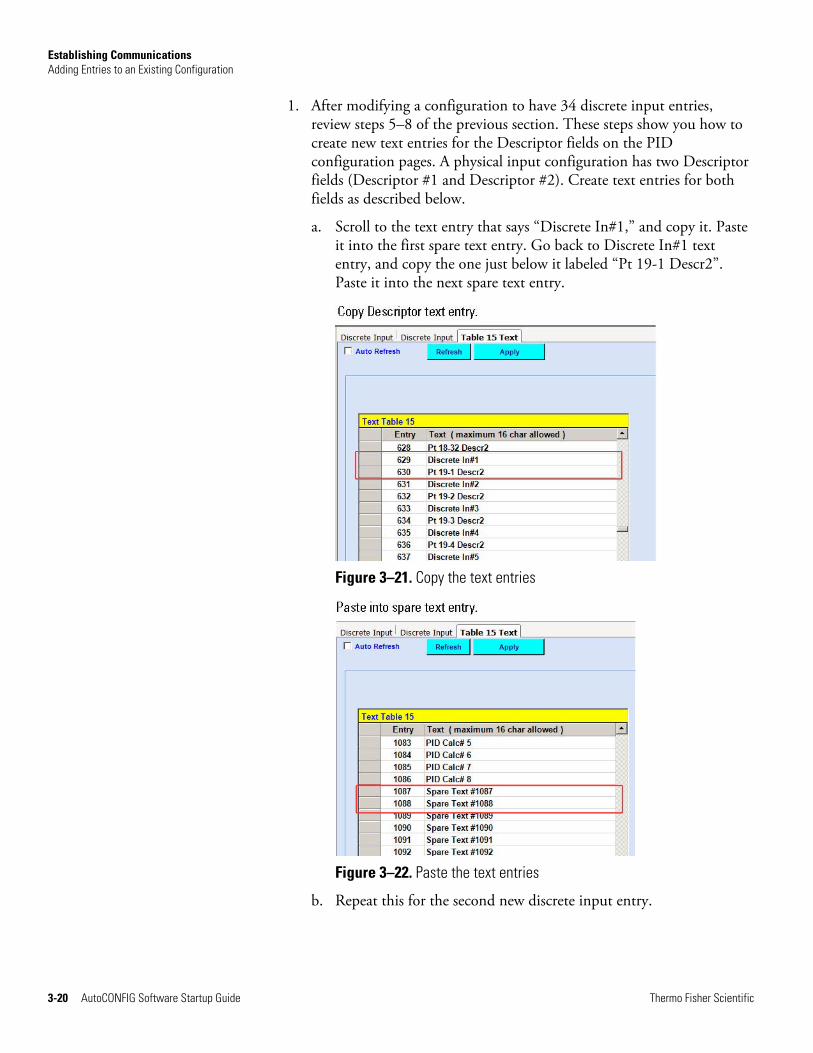
1. After modifying a configuration to have 34 discrete input entries, review steps 5–8 of the previous section. These steps show you how to create new text entries for the Descriptor fields on the PID configuration pages. A physical input configuration has two Descriptor fields (Descriptor #1 and Descriptor #2). Create text entries for both fields as described below.

a. Scroll to the text entry that says “Discrete In#1,” and copy it. Paste it into the first spare text entry. Go back to Discrete In#1 text entry, and copy the one just below it labeled “Pt 19-1 Descr2”. Paste it into the next spare text entry.

Figure 3–21. Copy the text entries

Figure 3–22. Paste the text entries

b. Repeat this for the second new discrete input entry.



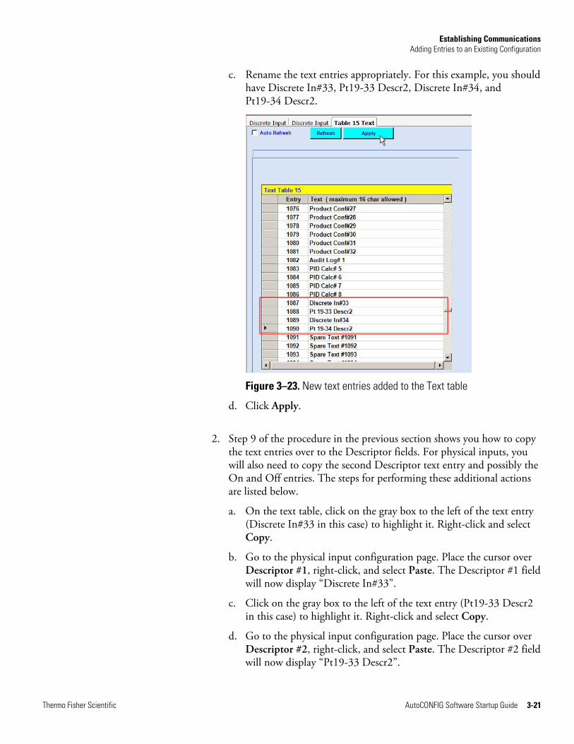
c. Rename the text entries appropriately. For this example, you should have Discrete In#33, Pt19-33 Descr2, Discrete In#34, and Pt19-34 Descr2.

Figure 3–23. New text entries added to the Text table

d. Click Apply.

2. Step 9 of the procedure in the previous section shows you how to copy the text entries over to the Descriptor fields. For physical inputs, you will also need to copy the second Descriptor text entry and possibly the On and Off entries. The steps for performing these additional actions are listed below.

a. On the text table, click on the gray box to the left of the text entry (Discrete In#33 in this case) to highlight it. Right-click and select Copy.

b. Go to the physical input configuration page. Place the cursor over Descriptor #1, right-click, and select Paste. The Descriptor #1 field will now display “Discrete In#33”.

c. Click on the gray box to the left of the text entry (Pt19-33 Descr2 in this case) to highlight it. Right-click and select Copy.

d. Go to the physical input configuration page. Place the cursor over Descriptor #2, right-click, and select Paste. The Descriptor #2 field will now display “Pt19-33 Descr2”.



e. The physical discrete input pages have On Descriptor Text and Off Descriptor Text fields. Go to Table #15 and locate the On and Off text entries. They are usually located around item 20.

Figure 3–22. On and Off text entries

f. Click on the gray box to the left of the On text entry to highlight it. Right-click and select Copy.

g. Go to the physical input configuration page, place the cursor over On Descriptor Text, right-click, and select Paste.

h. Click on the gray box to the left of the Off text entry to highlight it. Right-click and select Copy.

i. Go to the physical input configuration page, place the cursor over Off Descriptor Text, right-click, and select Paste.

Note Be sure to click Apply after copying the text entries. ▲

Figure 3–23 shows what the screen will look like with the new text entries connected.



Figure 3–23. Example of additional physical discrete input entry with new text entries connected

3. Since this is a physical input, you do not need to follow step 10 of the main procedure, which connects the calculation to a thread. You can now save the configuration with the additional physical input entries.


Establishing Communications Special PC Setup for AutoCONFIG Software

Special PC Setup for

AutoCONFIG Software

If you notice that the AutoCONFIG software is running slowly or you receive COMM errors, the PC may not be set up to use a greater share of the processor time to run background services. Follow the procedure below to determine if this may be the cause of the communication problems.

Note This procedure changes a PC system setting. This setting may remain changed, as it should not affect other programs you run. ▲

1. On the PC desktop, right-click the My Computer icon and select Properties. The System Properties screen will open. You can also access this screen by selecting Start > Control Panel > System.

Figure 3–24. System Properties screen



2. Click the Advanced tab, and under Performance, click Settings.

Figure 3–25. Selecting Performance Settings

3. Click the Advanced tab on the Performance Options screen. Check what is selected under Processor scheduling. Select Background services if not already selected. Click Apply.

Figure 3–26. Changing the system performance setting




4. Click OK to return to the desktop.

5. Run the software to determine if changing this setting has resolved the communication problem.

Chapter 4

Configuring a Meter Run with the Measurement Config Wizard

The Measurement Config wizard helps you configure gas and/or liquid runs easily by presenting the screens in a logical order, taking you through each configuration step required. If you want to configure one meter run, a DP meter run for example, expand the 38-Differential Pressure Flow heading, right-click over an entry, and select Config Wizard. This wizard will take you through the configuration process for one meter run only. To configure multiple runs, select the Measurement Config wizard from the Tools menu.

Overview

This chapter provides instructions on using the Measurement Config wizard for multiple runs in two sections: one for gas runs (DP or AGA 7 flow) and one for liquid flow runs.

Note Liquid flow calculations are available with the AutoPILOT PRO flow computer if you do not need frequency based densitometer inputs or require proving capabilities. ▲

Note This section does not provide information on each parameter. For this level of detail, reference the Measurement Config wizard section in the software help system. ▲


Configuring a Meter Run with the Measurement Config Wizard For Gas Meter Runs

Follow the procedure in this section to configure DP and/or AGA 7 meter runs using the Measurement Config wizard.

For Gas Meter Runs

1. Go to Tools > Measurement Config Wizard. The software will ask if you want to run the Measurement Config wizard. Click OK to continue.

2. If you are not connected to an instrument (offline connection), the screen shown below will be displayed. Select DP Flow or AGA 7 Flow and the number of runs to configure. If you want to configure gas quality for historical archives, check the Change Configuration History box, and select the type of gas quality to use. When you are ready to continue, click Next.

If you are connected to an instrument, the Gas Quality Selection for Historical Archive blocks will not be displayed (gas quality cannot be configured from within the wizard).

Figure 4–1. Selecting the meter runs and gas quality

3. The wizard will inform you that the software is working and ask you to wait. This may take a few minutes.



4. When the Set Unit Date & Time screen appears, select Automatic to use the time and date as set in the PC, or select Manual to enter the time and date manually. Click Apply.

Figure 4–2. Setting the unit time and date



5. On the DP Flow page, configure the static and gas quality data for the first meter run. Going with the example above, run #1 is a DP run that will be referred to as DP Flow Calc#1.

Figure 4–3. Configuring static data and gas quality for DP Flow Calc#1

Note For this example, the DP runs will be configured first and the AGA 7 run last. If you selected AGA 7 meter runs only in the previous screen, skip the DP run configuration steps and go to step 9. ▲



6. On the DP Flow Factors page, enable any required flow factors and set the engineering units for DP Flow Calc#1. When you have completed this page, click Next.

Note More on these factors, including the equations used, can be found in the software help system. ▲

Figure 4–4. Configuring DP Flow Calc#1 factors and engineering units



7. The wizard will read the current I/O connections from the RTU and display them on the DP Flow Connections page. Confirm the connections, and click Download & Next to continue with the configuration process. If you click the Download & Exit button, the wizard will download the current run configuration and close. You will return to the main AutoCONFIG window. When you click either of these buttons, you will be notified by the software that the calculation will be configured if you continue. Select Yes to continue.

Figure 4–5. Connecting to physical inputs

8. If you clicked the Download & Next button in the previous step, one of two things will happen depending on where you are in the configuration process. If continuing with the example of two DP runs and one AGA 7 run, there are two runs left to configure. The next screen will be the DP Flow screen for the second DP run (DP Flow CAlc#2). Return to step 5. After configuring the second DP run (when you reach this point again), the first screen for the last run (an AGA 7 run) will be displayed. Go to step 9. If you selected only one run or if this is the last run to be configured, the software will ask if you want to run the Calibration wizard. Click Yes to run the wizard. If you click No, the software will display that configuration is complete. The screen will close, and you will return to the main AutoCONFIG window.



9. On the AGA7 Flow screen, configure the static and gas quality data for the AGA 7 meter run.

Figure 4–6. Configuring AGA7 static and gas quality data



10. On the AGA7 Flow Factors page, enable any required flow factors and set the engineering units for AGA7 meter run. When you have completed this page, click Next.

Figure 4–7. Configuring AGA7 factors and engineering units



11. On the AGA7 Flow Connections screen, select whether this configuration is for an AGA 7 turbine run or AGA 7 auto-adjust. The wizard will read the current I/O connections from the RTU and display them here. Confirm the connections, and click Download & Next to continue with the configuration process. If you click the Download & Exit button, the wizard will download the current run configuration and close. You will return to the main AutoCONFIG window. When you click either of these buttons, you will be notified by the software that the calculation will be configured if you continue. Select Yes to continue.

Figure 4–8. Connecting to physical inputs

12. If there are more runs to configure, click the Download & Next button. The next screen will be the static data and GQ screen for the next run. If you have configured the final run, click the Download & Exit button. The software will ask if you want to run the Calibration wizard. Click Yes to do so. If you click No, the software will display that configuration is complete. The screen will close, and you will return to the main AutoCONFIG window.


Configuring a Meter Run with the Measurement Config Wizard For Liquid Flow Runs

Follow the procedure in this section to configure liquid flow runs using the Measurement Config wizard.

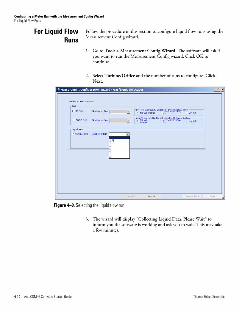
For Liquid Flow Runs

1. Go to Tools > Measurement Config Wizard. The software will ask if you want to run the Measurement Config wizard. Click OK to continue.

2. Select Turbine/Orifice and the number of runs to configure. Click Next.

Figure 4–9. Selecting the liquid flow run

3. The wizard will display “Collecting Liquid Data, Please Wait” to inform you the software is working and ask you to wait. This may take a few minutes.



4. When the Set Unit Time & Date screen appears, select Automatic to use the time and date as set in the PC, or select Manual to enter the time and date manually. Click Apply.

Figure 4–10. Setting the unit time and date



5. On the first configuration page, enter the run descriptions, select whether a turbine or orifice flow type, and set the engineering units. When you have completed this page, click Next.

Figure 4–11. Setting general run descriptions, type, and engineering units

6. If you selected a turbine flow type in the previous screen, the screen shown in Figure 4–12 will be displayed. Select a single or dual turbine meter pickup pulse, enter the meter K Factor, and select whether meter linearization should be enabled. Click Next and continue to the next step.

If you selected an orifice meter, the screen shown in Figure 4–13 will be displayed. Select a single, dual, or triple DP input, and then enter the mid and high DP switch values. Click Next and continue to the next step.



Figure 4–12. Screen for turbine flow type

Figure 4–13. Screen for orifice flow type



7. If you enable the meter linearization function, enter up to ten flow meter pulse frequencies (in Hz). Each frequency must be greater than the previous frequency. When ready, click Next.

Figure 4–14. Entering the flow meter pulse frequencies



8. If you are not going to measure density, select None in the Density Type field, and click Next. Go to step 9. If measuring density, select the density type and the source of temperature and pressure. Click Next.

Figure 4–15. Density configuration screen



9. The wizard will read the current I/O connections from the RTU and display them here. Confirm the connections, and click Download & Next to continue with the configuration process. If you click the Download & Exit button, the wizard will download the current run configuration and close. You will return to the main AutoCONFIG window. When you click either of these buttons, you will be notified by the software that the calculation will be configured if you continue. Select Yes to continue.

Once you have made the necessary connections, click Next.

Figure 4–16. Physical input connections

10. The software will ask you to wait while it downloads the data.



11. The Product Setup screen gives you the opportunity to configure products. If you do not want to do this, select No in the Setup Products Now drop-down, and click Next. Skip the remainder of this step.

If you want to configure a product now, select Yes in the Setup Products Now drop-down, followed by how many products you want to configure. Click the Next button, and the setup screen for the first product will appear (Figure 4–18). When you complete this page, click Next, and the configuration page for the next product will open. Continue this process until you have set up each product.

Figure 4–17. Product Setup screen



Figure 4–18. Configuration screen for first product

12. If you do not need to configure a densitometer, select No in the Setup Densitometers Now drop-down, and click Next. Go to step 13.

If you want to set up a density calculation, select Yes in the Setup Densitometers Now drop-down. Click Next, and the configuration page for the first density calculation appears (Figure 4–20). When you complete this page, click Next, and the configuration page for the next density calculation will open. Continue this process until you have configured each densitometer.



Figure 4–19. Densitometer Setup screen

Figure 4–20. Configuration screen for the first densitometer




13. Densitometer configuration is the final part of a liquid flow run configuration. After you complete step 12 and click Next, the software will ask if you want to run the Calibration wizard. Click Yes to run the wizard. If you click No, the software will display that configuration is complete, and you can close the window to return to the main AutoCONFIG window.

Chapter 5

Gas Quality

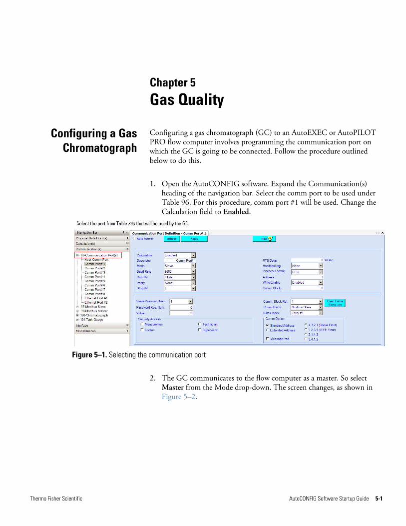
Configuring a gas chromatograph (GC) to an AutoEXEC or AutoPILOT PRO flow computer involves programming the communication port on which the GC is going to be connected. Follow the procedure outlined below to do this.

Configuring a Gas Chromatograph

1. Open the AutoCONFIG software. Expand the Communication(s) heading of the navigation bar. Select the comm port to be used under Table 96. For this procedure, comm port #1 will be used. Change the Calculation field to Enabled.

Figure 5–1. Selecting the communication port

2. The GC communicates to the flow computer as a master. So select Master from the Mode drop-down. The screen changes, as shown in Figure 5–2.


Gas Quality Configuring a Gas Chromatograph

Figure 5–2. Master mode configuration page

3. Configure the communication port. For this example, the GC being connected will communicate via RS232 communication with the following port settings.

Note The following information is for this example. The port configuration for the GC should match the port configuration of the instrument to which the GC will be connected. ▲

a. Baud Rate: 1200

b. Data Bit: 7

c. Parity: Even

d. Stop Bit: 1

e. Protocol: ASCII

f. Comm Block Ref, Comm Block, and Block Index:

Set the block reference for the port. If you are setting up the first task for this port, set the Comm Block Ref to 1. If you are setting up the tenth task for this port, set it to 10, etc.

Since you are configuring the port for a GC, select chromatograph from the Comm Block drop-down.

Select the block index (entry #) that corresponds to the communications block you chose.

4. Click Apply.


Gas Quality Gas Quality without a GC


The GC can now communicate with the flow computer through the configured communication port. To view the live GC analysis, go to Communication(s) > 100-Chromatograph. Select the chromatograph stream that corresponds to the block index you selected in the above procedure. For example, if you selected Entry #1, the GC data will go to Chrom Stream #1. Table #100 Chrom Stream #1 (for this example) will send GC data internally to Table #128 under the respective GQ data block.

Gas Quality without a GC

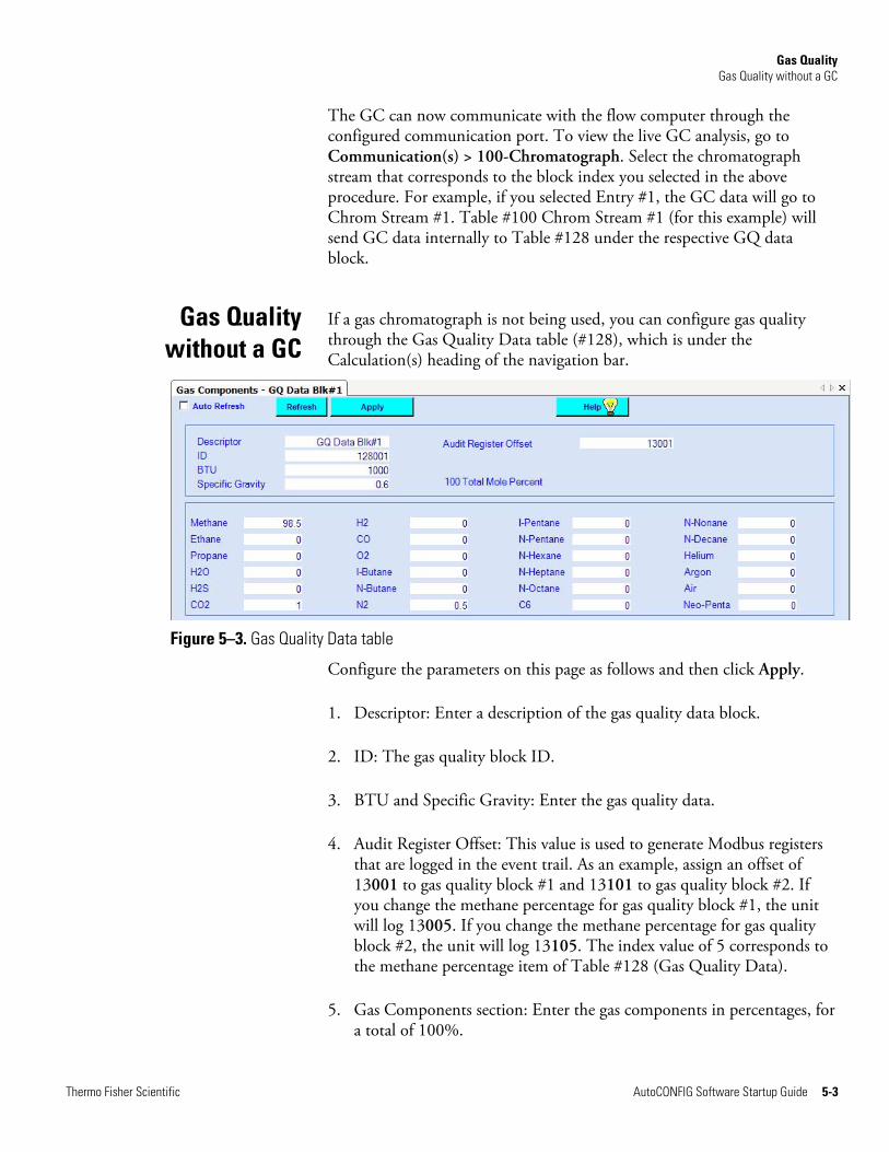
If a gas chromatograph is not being used, you can configure gas quality through the Gas Quality Data table (#128), which is under the Calculation(s) heading of the navigation bar.

Figure 5–3. Gas Quality Data table

Configure the parameters on this page as follows and then click Apply.

1. Descriptor: Enter a description of the gas quality data block.

2. ID: The gas quality block ID.

3. BTU and Specific Gravity: Enter the gas quality data.

4. Audit Register Offset: This value is used to generate Modbus registers that are logged in the event trail. As an example, assign an offset of 13001 to gas quality block #1 and 13101 to gas quality block #2. If you change the methane percentage for gas quality block #1, the unit will log 13005. If you change the methane percentage for gas quality block #2, the unit will log 13105. The index value of 5 corresponds to the methane percentage item of Table #128 (Gas Quality Data).

5. Gas Components section: Enter the gas components in percentages, for a total of 100%.


Chapter 6

System Status & System Control Tables

The System Status and System Control tables allow you to view important system information and set basic system parameters. Access both tables through the Miscellaneous heading on the navigation bar.

System Status (Table #30)

stem Status (Table #30)

The System Status table has two tabs: General and System I/O Counts.

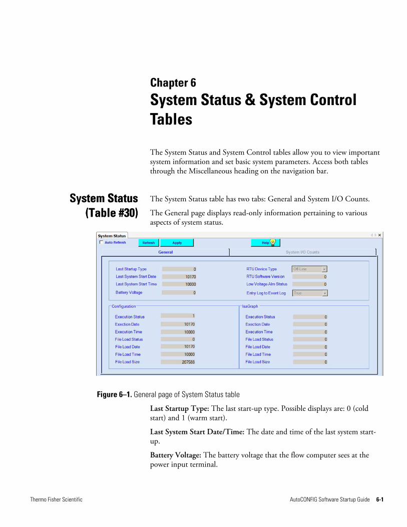
The General page displays read-only information pertaining to various aspects of system status.

Figure 6–1. General page of System Status table

Last Startup Type: The last start-up type. Possible displays are: 0 (cold start) and 1 (warm start).

Last System Start Date/Time: The date and time of the last system start-up.

Battery Voltage: The battery voltage that the flow computer sees at the power input terminal.


System Status & System Control Tables System Status (Table #30)

RTU Device Type: Displays the type of device currently connected.

RTU Software Version: The software version of the currently connected device.

Low Voltage Alarm Status: Displays whether a low voltage alarm is currently active. Possible displays are: 0 (alarm clear) and 1 (alarm active).

Entry Log to Event Log: This flag indicates that an entry has been logged to the system error log and should be retrieved by the Host/user, etc. Reset the flag by issuing a "2468" numerical command into the Configuration Load Control field in Table #31.

Configuration block

Execution Status: The status of the configuration. Possible displays are: 0 (configuration idle), 1 (configuration running), and 2 (configuration failure).

Execution Date/Time: The date and time the configuration file was executed.

File Load Status: The configuration file load status. Possible displays are: 0 (no configuration loaded), 1 (configuration loaded), 2 (configuration executed), and 3 (configuration generated).

File Load Date/Time: The last date and time the configuration file was loaded.

File Load Size: The size of the configuration file.

IsaGraph block

Execution Status: The status of the IsaGraph. Possible displays are: 0 (IsaGraph idle), 1 (IsaGraph running), and 2 (IsaGraph failure).

Execution Date/Time: The date and time the IsaGraph file was executed.

File Load Status: The IsaGraph file load status. Possible displays are: 0 (no IsaGraph file loaded), 1 (IsaGraph file loaded), and 2 (IsaGraph file executed).

File Load Date/Time: The last date and time the IsaGraph file was loaded.

File Load Size: The size of the IsaGraph file.


System Status & System Control Tables System Status (Table #30)

As on the General page, most of the items on the System I/O Counts page are read-only. The I/O Board Failure Alarm field displays the status of the I/O board failure alarm, where 0 is alarm clear and 1 is alarm active. This page also displays the following system information:

● Number of I/O boards installed

● Types of inputs and outputs

● Number of dynamic and static RAM pages, Flash, and EEPROM pages

● Number of communication ports

Additionally, you can view the size of historical and audit/alarm logs. Select the log you want, and the file size is displayed.

Figure 6–2. System I/O Counts page


System Status & System Control Tables System Control (Table #31)

System Control (Table #31)

ystem Control (Table #31)

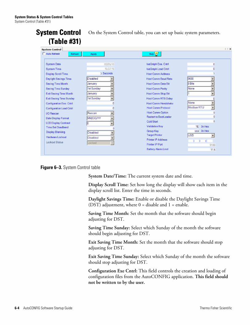
On the System Control table, you can set up basic system parameters.

Figure 6–3. System Control table

System Date/Time: The current system date and time.

Display Scroll Time: Set how long the display will show each item in the display scroll list. Enter the time in seconds.

Daylight Savings Time: Enable or disable the Daylight Savings Time (DST) adjustment, where 0 = disable and 1 = enable.

Saving Time Month: Set the month that the software should begin adjusting for DST.

Saving Time Sunday: Select which Sunday of the month the software should begin adjusting for DST.

Exit Saving Time Month: Set the month that the software should stop adjusting for DST.

Exit Saving Time Sunday: Select which Sunday of the month the software should stop adjusting for DST.

Configuration Exe Cntrl: This field controls the creation and loading of configuration files from the AutoCONFIG application. This field should not be written to by the user.



Configuration Load Cntrl: This is the command used to load the current running configuration into an internal data storage location that can be accessed by the software for retrieval and storage on a PC. This command is automatically utilized when a user selects to Upload Configuration from RTU from the Files menu or clicks the corresponding icon on the toolbar.

I/O Rescan: You can force the software to rescan the I/O boards to establish an I/O point count. This is typically performed after you have installed a new I/O board.

Date Display Format: Select how you want the software to display the date (MM/DD/YY, DD/MM/YY, YY/MM/DD).

LCD Display Contrast: You can adjust the contrast of the LCD from the front panel of the instrument or from this field. Increase the number to increase the contrast.

Time Set Deadband: This deadband is used when synchronizing the unit's internal clock with a host system's clock. If the time difference is within the deadband, the unit will not set its internal clock automatically. For instance, if the deadband is set to 60 seconds, the unit will not automatically synchronize its internal clock with the host clock unless the time difference is more than one minute.

Display Blanking: If enabled, the unit will not scroll data on the LCD unless a password is entered through the keypad. If disabled, the unit will scroll data whenever a cable is plugged into the local port or a key is pressed on the keypad.

Hardware Lockout: The user has the ability to lock out any user parameter changes based on the status of Digital Input #1. This is achieved by using the Hardware Lockout and Lockout Status parameters. When the Hardware Lockout parameter is set to Enable, and Digital Input #1 is “On” (as indicated by the Lockout Status parameter changing to Locked), the unit does not allow changes to any parameters. This includes changes attempted via any serial port, Ethernet, and the keypad. Note that when this feature is enabled, Digital Input #1 is reserved for this function and thus is not available for general use. This feature was designed specifically to meet the Measurement Canada requirement for sealing the flow computer. If this feature is not desired, leave the Hardware Lockout parameter set to Disabled, the default setting. In this case, Digital Input #1 is then available for general use.

Lockout Status: See Hardware Lockout.

IsaGraph Exe Cntrl: This field controls the creation and loading of configuration files from the IsaGraph. This field should not be written to by the user.

IsaGraph Load Cntrl: This field is for future development.




Host Comm Address: Enter the host address. This entry will override the entry made in the address field of Table #96 (Communications Ports).

Host Comm Baud Rate/Data Bit/Parity/Stop Bit: Set the communications parameters for the host port. These entries will override the entry made in the address field of Table #96 (Communications Ports).

Host Comm RTS Delay: Enter the time in milliseconds that the instrument should wait after raising a Request to Send on the host port before transmitting a message. This entry will override the entry made in the address field of Table #96 (Communications Ports).

Host Comm Handshake: Select the method by which data is transferred from the modem to the communications port. This entry will override the entry made in the address field of Table #96 (Communications Ports). Options are: None (no handshaking) and RTS/CTS (Request To Send/Clear To Send handshaking).

Host Comm Protocol: If necessary, select the slave mode protocol format (Modbus ASCII or Modbus RTU).

Host Comm Option: This field is for future development.

Cold Start: This field provides another way to perform a cold start. Enter 12345.0 and click Apply.

Validation Key and Group Key: These keys are used together to enable software features that are purchased separately from the hardware. For example, if an AutoPILOT PRO flow computer is originally purchased with the plunger lift function, these keys will be entered at the factory, and the unit will arrive with plunger lift available. If the plunger lift function is purchased after the original order of the unit, you will receive Validation and Group keys that must be entered here to enable the function.

Target Printer: To print reports on a printer that is connected via a USB port, select USB. If the connection is through an Ethernet connection, select Ethernet.

Printer IP Address: Enter the printer IP address. You can usually find the IP address by going to the Windows Start menu and selecting Printers and Faxes.

Printer IP Port: The IP port for the printer.

Battery Alarm Limit: If the system battery falls to the voltage value entered here an alarm will be logged.

Chapter 7

AutoCONFIG Software & the Help System

The AutoCONFIG software is a powerful tool, and with the meter run calculations configured and running, you can explore the software’s other capabilities.

Using the Software

he Software

There are three ways to navigate through the software: the main menu, the toolbar, and the navigation bar. These items are explained in the AutoCONFIG software help system.

Figure 7–1.

Using the Help System

Using the Help System

The help system includes information on the tools, calculations, and features in the AutoCONFIG software.

You can open the help system by clicking the Knowledge Base icon on the toolbar.

Knowledge Base icon


AutoCONFIG Software & the Help System Using the Help System

When opened, the help system appears as a tri-pane window. The Contents pane is on the left and contains the system's table of contents, index, and search function.

● Table of contents: Provides an outline of the material contained in the help system.

Figure 7–2. Table of contents

● Index: Use the index to find topics for a keyword (or words) that you enter.

● Search: The search function is similar to the index in that you enter a keyword and a list of topics is displayed. It is a broader function, however, and displays every topic in which that keyword is used.

● Glossary: The glossary contains important terms and their definitions.


AutoCONFIG Software & the Help System Page Level Help


Page Level Help ge Level Help The AutoCONFIG software provides page level help. For example, if you have Table #33 open to configure a PID, click the Help button to open the help file for that page only.

Figure 7–3. Getting help for a specific page in the software

Printing the Help System

Printing the Help System

There are several ways to print the help system.

1. To print the topic that is currently displayed, right click anywhere on the Topic pane and select Print or click the print icon. Note that this method will only print the current topic. It will not print any drop-down text unless you display it first.

2. For printer friendly versions and/or to print multiple topics or sections, open the book labeled "Supplemental Material" (in the contents). From there, you can download the desired PDF file to your computer and print it or save it for reference.

3. On some topic pages, you will see a printer icon at the top. Click it to open a PDF/printer friendly version of just that topic. This improvement is in ongoing at the time of this release and is not available for all topics.


Thermo Fisher Scientific AutoCONFIG Software Startup Guide GLOSSARY-1

Glossary

AutoEXEC flow computer The Thermo Scientific hybrid, multi-run flow computer and remote telemetry unit for natural gas and / or petroleum liquids.

AutoPILOT PRO flow computer The Thermo Scientific six-run gas flow computer and remote telemetry unit.

baud The speed measurement for communication that indicates the number of bit transfers per second.

chromatograph function Consists of a Modbus master that polls a Danalyzer gas chromatograph for its molar percent components, BTU, and specific gravity.

CTS Clear to send.

CTS wait Amount of time in milliseconds the program should wait for the CTS signal to be returned from the software's local communications device after raising Request to Send.

data bits Measurement of the actual data bits in a transmission.

DP Differential pressure.

EU Engineering unit

Fpv Supercompressibility factor calculated by using AGA 8.

Fpwl Factor used to correct for the effect of local gravity on the weights of a deadweight calibrator.

Fwl Local gravitational correction factor.

Fwv See Water Vapor Factor.

gas components table Table used in AutoCONFIG software to enter gas quality data if a chromatograph is not being used.

GC Gas chromatograph.

GQ Gas quality.

K-Factor The number of pulses per unit volume.

measurement config wizard A tool that enables you to configure differential pressure meter runs, turbine meter runs, and/or liquid flow runs easily by presenting the screens in a logical order, taking you through each configuration step required.

RTC Real-time clock.

RTS Request to send.

RTS fall Amount of time in milliseconds the program should hold the RTS signal as high after sending the last data byte to the RTU.

RTS rise Also referred to as "Radio Key Delay". Amount of time in milliseconds the RTS signal should be raised before the program sends the first data byte to the RTU.

RTS wait Amount of time in milliseconds the program should delay raising an RTS after receiving the last data byte from the RTU.

SP Static pressure.

stop bits Used to signal the end of communication for a single packet.

Water Vapor Factor A direct multiplier into the flow equation that compensates for any water vapor in the system.


Index

A adding entries to a configuration, 3-12–3-21 AGA 7 meter run

configuration using Measurement Config wizard, 4-1–4-9

AutoCONFIG software, 1-1, 7-1–7-3 establishing communications, 3-1–3-11 help system, 7-1–7-3 installation, 2-3

AutoEXEC flow computer, 1-1 communication connections, 2-1–2-2

AutoPILOT PRO flow computer, 1-1 communication connections, 2-3

C calculation thread allocation table #32, 3-17–3-19 chromatograph table #100, 5-3 Communication Parameters screen, 3-1–3-11 communication ports table #96

configuration for gas chromatograph, 5-1–5-3 configuration of TCP/IP for remote connection, 3-8

communications, 3-1–3-11 connections for AutoEXEC flow computer, 2-1–2-2 connections for AutoPILOT PRO flow computer, 2-3 establishing a local connection, 3-5 establishing a remote connection via TCP/IP, 3-4 establishing an off line connection, 3-2 port configuration for gas chromatograph, 5-1–5-3 troubleshooting, 3-24–3-26

configuration modifying a, 3-12–3-21 of communication parameters, 3-1–3-11 of communication port for gas chromatograph, 5-1–5-3 of gas meter runs with Measurement Config wizard, 4-

1–4-9 of gas quality data

with gas chromatograph, 5-1–5-3 without a gas chromatograph, 5-3

configuring communication parameters, 3-1–3-11 communication port for gas chromatograph, 5-1–5-3 gas meter runs with Measurement Config wizard, 4-1–

4-9 gas quality data

with gas chromatograph, 5-1–5-3 without a gas chromatograph, 5-3

D daylight savings time (DST), 6-4 DP meter run

configuration using Measurement Config wizard, 4-1–4-9

DST. See daylight savings time.

G gas chromatograph, 5-1–5-3 gas meter run configuration, 4-1–4-9 gas quality data table #128, 5-3 GC. See gas chromatograph.

I installation, 2-1–2-3

hardware, 2-1 of AutoCONFIG software, 2-3

IP address, 3-4 setup for remote communications, 3-8–3-10

M Measurement Canada, 6-5 Measurement Config wizard

for gas meter runs, 4-1–4-9 modifying a configuration, 3-12–3-21

O off line connection, 3-2

Thermo Fisher Scientific AutoCONFIG Software Startup Guide INDEX-1

Index

INDEX-2 AutoCONFIG Software Startup Guide Thermo Fisher Scientific

P product CD, 1-1, 2-3

R receiving

items included with shipment, 1-1 remote connection, 3-4

S System control table #31, 6-4–6-6 System status table #30, 6-1–6-3

T Table #100 chromatograph, 5-3 Table #128 gas quality data, 5-3

Table #15 text, 3-2, 3-14–3-17 copying text entries, 3-16 editing text entries, 3-14–3-16

Table #30 system status, 6-1–6-3 Table #31 system control, 6-4–6-6 Table #32 calculation thread allocation, 3-17–3-19 Table #96 communication ports

configuration for chromatograph connection, 5-1–5-3 configuring the IP address for remote communications,

3-8–3-10 text table #15, 3-2, 3-14–3-17

copying text entries, 3-16 editing text entries, 3-14–3-16

turbine meter run configuration using Measurement Config wizard, 4-1–

4-9

Thermo Fisher Scientific81 Wyman StreetP.O. Box 9046Waltham, Massachusetts 02454-9046United States

www.thermofisher.com

Documents

Thermo Scientific AutoCONFIG Software Startup Guide