Embed Size (px)
Citation preview
1
THERMO-ECONOMIC ANALYSIS AND OPTIMIZATION OF THE STEAM ABSORPTION
CHILLER NETWORK PLANT
Farshad Panahizadeh1 ,Mahdi Hamzehei
1*, Mahmood Farzaneh-Gord
1, 2,Alvaro Antonio Ochoa
Villa1, 3
1Department of Mechanical Engineering, Ahvaz Branch, Islamic Azad University, Ahvaz, Iran
2Department of Mechanical Engineering, Ferdowsi University of Mashhad, Mashhad, Iran
3Federal Institute of Technology of Pernambuco, Av. Prof. Luiz Freire, 00, CEP:50740-540, Recife,
PE, Brazil
*Correspond author email address: [email protected];[email protected]
Absorption chillers are one of the most used equipment in industrial,
commercial, and domestic applications. For the places where high cooling is
required, they are utilized in a network to perform the cooling demand. The
main objective of the current study was to find the optimum operating
conditions of a network of steam absorption chillers according to energy and
economic viewpoints. Firstly, energy and economic analysis and modeling of
the absorption chiller network were carried out to have a deep
understanding of the network and investigate the effects of operating
conditions. Finally, the particle swarm optimization search algorithm was
employed to find an optimum levelized total costs of the plant. The
absorption chiller network plant of the Marun Petrochemical Complex in
Iran was selected as a case study. To verify the simulation results, the
outputs of energy modeling were compared with the measured values. The
comparison with experimental results indicated that the developed model
could predict the working condition of the absorption chiller network with
high accuracy. The economic analysis results revealed that the levelized
total costs of the plant is 1730 $/kW and the payback period is three years.
The optimization findings indicated that working at optimal conditions
reduces the levelized total costs of the plant by 8.5%, compared to the design
condition.
Keywords: Absorption chiller network, Energy and economic analysis,
Levelized total costs, Particle swarm optimization
1. Introduction
Absorption chillers represent an exciting alternative to the conventional vapor-compression
chillers because they can supply cooling without high electrical consumption [1-3]. The mechanical
compressor of a compression chiller is indeed substituted by a thermal compressor, where the
refrigerant vapor at the outlet of the evaporator is first absorbed in an absorbent solution, pumped to
the higher-pressure level, and then desorbed again in the generator [4, 5]. To drive this process, a low-

2
temperature heat source is necessary at the generator [6-9]. The absorption refrigeration cycle is
gaining considerable attention because it can make fair use of low-grade waste heat for cooling
demand and employ eco-friendly refrigerant [10, 11]. It is evident the uses of the thermo-economic
analysis to verify the viability of the cogeneration systems have been used and applied along with
different thermal plants [12, 13], aiming the best proposal to generate steam, electricity, and chilled
water for the ice factory industry [14], to generate enough energy for achieving the demand of the
swimming pool indoor buildings [15] or even to generate air cooling and electricity for buildings in
the university [16, 17]. Since the thermo-economic analysis aims to investigate the energetic technical
parameters and also the financial indices to estimate if any thermal plant would be feasibly or not [18],
the needs to search for the ideal input configuration in terms of the energetic and economic domain
have been mentioned in many studies on polygeneration systems, as it could be seen in the literature
[19, 20]. In this context, using different technical methods to optimize the thermal systems have been
applied to find the best configuration for energetic and economic efficiency using the Four E
technique [21], artificial neural network [22], using the TRNSYS function to the optimization of the
economic index [23], MOPSO algorithm [24] or even combining different techniques of optimization
such as pessimistic and optimistic criteria [25]. Previously, Panahizadeh et al. [26] presented an
analogous study using the exergetic parameters as the basis of the optimization method trying to
minimize the exergy destruction by applying the particle swarm optimization algorithm; however, in
the present study, we aimed to use the financial parameters such as levelized total costs, net present
value, internal rate of return, and payback period as the basis of the objective function to the
optimization method. Hence, the main goal of this study was to implement an optimization analysis
with an energetic-economic view to find the best configuration for the network of the absorption
chiller to operate efficiently. Although extensive research has been done on thermo-economic analysis
of absorption chillers, insufficient research has been carried out on the absorption chiller network
plant. Also, the limited thermodynamic analysis of the absorption chiller network plant has been
carried out; however, to the best of the author's knowledge, no comprehensive analyses have been
done in identifying the optimum operation conditions of the absorption chiller network plant. To
bridge this gap, the main contributions of this state-of-the-artwork can be drawn as follows, proposing
a novel computer algorithm for simultaneous thermo-economic analysis of the absorption chiller
network plant, performing accurate and detailed energy and economic simulation of the mentioned
plant, evaluating the influence of changing operating conditions like cooling tower water temperature
and steam temperature on the levelized total costs of the absorption chiller network plant, applying the
two most important economic methods of payback period (PP) and net present value (NPV) for
evaluating the mentioned plant, presenting a comprehensive sensitivity analysis for investigating the
effects of design parameters on assessment criteria of the plant mentioned above, and performing a
particle swarm optimization search algorithm for finding the optimal levelized total costs of the stated
plant.
2. Description of the absorption chiller network plant
An absorption chiller network (ACN) includes more than one chiller that work together in a
series or parallel arrangement to produce the desired cooling capacity. Apart from absorption chillers,
the absorption chiller network plant (ACNP) should have also additional equipment including the
main boiler, chilled water storage tank, cooling tower, cooling tower water pump, chilled water pump
3
and air handling or heat exchangers to generate required cooling demand. In this research, the ACNP
used for the cooling process in the Mono-Ethylene Glycol (MEG) factory of Marun Petrochemical
Complex (M.P.C.) in Iran is selected as a case study as shown in Figure 1. The plant consists of four
single effect steam absorption chillers with a cooling capacity of 4775 kW, two forced draft fan
cooling towers, a storage tank, cooling tower pumps, and chilled water pump. Also, in this study, it
was assumed the steam boiler produced required steam of four chillers with a capacity of 44 tons of
steam per hour with 1.5 bar pressure and consumed natural gas.
Figure 1. Schematic of the ACNP: case study
3. Thermo-economic and optimization modeling of the ACNP
This section shows the energy analysis, economic and optimization modeling of the absorption
chiller network plant
3.1. The energy analysis of the absorption chiller network plant
For evaluating the performance of a system from different viewpoints, it is necessary to perform
the energy analysis of the whole system. The general forms of the mass and energy balance equations
for a control volume at steady state flow are expressed as follows [27]:
∑ ∑
∑
∑
(1, 2)
In which , h, and represents the mass flow rate, specific enthalpy, heat power, and
mechanical power, respectively. Also, the subscripts i and o are related to the inlet and outlet streams
of the control volume. For concerned ACNP the final form of the energy balance equations for each
component is described in Table 1. In the following equations, indexes 1 to 20 are stream numbers as
shown in Figure 1.
Table 1. Energy balances of the ACNP
Equipment Equation
Boiler
(3)
Cooling tower
( )
( )
(4,5)
(6,7)
(8)

4
( )
ACN (9)
HX200 HX300 (10)
(11)
Cooling
tower
pump
Chilled
water
pump
(12)
(13)
Cooling tower fan
(14)
The variables , and are boiler heat input in kW, fuel mass flow rate in kg/s, fuel
lower heat value in kJ/kg and combustion efficiency, respectively. The variables , h, CPa, T, , ,
and are mass flow rate in kg/s, specific enthalpy in kJ/kg, specific heat at a constant
pressure of air in kJ/(kg.°C), temperature in °C, water vapor enthalpy in kJ/kg, absolute humidity in
kgH2O/kgdryair, water saturation pressure in kPa, atmospheric pressure in kPa and the relative humidity
of the air, respectively. The variables , , and are chilled water flow rate in
kg/s, the specific heat at constant pressure of water in kJ/(kg.°C), chilled water inlet and outlet
temperatures in °C, respectively. The variables are the input
work of the absorption chiller network in kW, the input work of cooling water pump in kW, cooling
water network inlet flow rate in kg/s, gravity acceleration in m/s2, cooling water pump head in km and
cooling water pump efficiency, respectively. Also, the variables are inlet
airflow rate in kg/s, cooling tower fan pressure difference in kPa, inlet air density in kg/m3 and cooling
tower fan efficiency, respectively.
The COPACN with M chillers and The COPACNP are defined by equations 15 and 16 [26]:
∑ ( )
(15,16)
Where , are a total cooling load of the network in kW, ACN’s generators heat
input in kW, ACN’s pumps power input in kW, ACNP’s pumps power input in kW, respectively.
3.2. Economic analysis
Economic analysis includes the estimation of different fixed and operating costs. Here, a
comprehensive economic analysis is done, which involves all of the important financial variables. The
fixed costs ( ) of the project include the investment costs of the system ( ) as shown in Table 2,
and the costs of installing the system components and their related piping ( ). Usually,
is considered between 5 to 15% of . In this study, it was assumed 10%
of [23].
Table 2. Cost functions of various components of the ACNP
System
Equipment Cost Function Ref.
System
Equipment Cost Function Ref.
Absorption
chiller ZAC =122.2 ($/kW) [36]
Pump
(
) ($) [28]
Storage tank ZST =290 ($/m3) [35] Boiler ZB=Ton of Steam×6500 ($) [29]
Cooling
Tower
( ) (
) ($) [28]
The operating cost ( ) of the system consist of the operating and maintenance cost ( ),
fuel and electricity cost ( ) ,and the environmental cost due to the penalty of the pollutant

5
emissions ( ). and N are the plant’s desired net produced power in kW and plant’s expected
lifetime in the year, respectively. Levelized total costs of the plant during the considered lifetime,
defined as below equation in $/kW [20]:
( )
(17)
∑
( ) ( ) (18, 19)
(20, 21)
In the above equations , , are fuel price in 10-6×($/GJ), electricity price
$/kWh, electricity consumption in kW and total working hours of the system each year, respectively.
The CO2 emission penalty cost of the ACNP related to electric and fuel consumption and calculated by
the following equation [34]:
( ) (22)
In the above equation are environmental tax factor and emission conversion
factor for electricity consumption from grid which are 0.024 $/kgCO₂ [21] and 0.571 kgco2/kWh [33].
Also, the variable is a CO2 flow rate and calculated by using natural gas combustion relation in
kgCO2/s. After completion of the plant’s economic assessment, the economic reliability of the plant is
evaluated through two important standard methods of Payback Period ( ) and Net Present Value
( ). Based on the definition, the is expressed as the length of time which takes to return all of
the investment costs [2].The amount of at the end of the system’s lifetime is calculated based on
below equation [11].
and ( ) ∑ ( )
(23, 24)
In which, the annual net saving money ( ), the inflation factor ( ) and the real discount factor
( ) are defined as the following equations [20].
(
)
(
)
(25, 26,
27)
Where is the total annual income of the plant, is the rate of inflation, DR is discount rate
and is the real interest rate. Also, stands for the -th year during the plant’s lifetime
and IRR is an internal rate of return [20].
∑
( )
(28)
In the economic analysis of the plant if:
NPV ˃0 and IRR˃DR, the plant investment is feasible. (29, 30)
3.3. Single objective optimization
Particle Swarm Optimization (PSO) algorithm has been used to search for optimal values of
decision variables of the concerned study. According to the set of benchmark test problems, it has
been shown that the PSO searching algorithm adopts in terms of both speed and memory requirements
has superior computational efficiency rather than a genetic algorithm (GA) in finding the global
optimal solution. PSO algorithm does not need evolution operators such as crossover and mutation
which are necessary for the GA algorithm. The parameters used for optimization in MATLAB by the

6
PSO algorithm in this study are shown in Table 3. The maximum number of iterations, the function
tolerance, and the maximum number of stall iterations were used as a stopping criterion of MATLAB
code. Inertia weight was used to define the percent of exploration (the ability to generate new
solutions) and exploitation (the ability to utilize current solutions) in the searching algorithm. Self and
social coefficients show the personal and global learning factors related to the self-cognitive
experience of particle and particle ability to learn from global. A swarm size is the number of particles
in the studied swarm.
Table 3. Parameters used for optimization in MATLAB for PSO algorithm
4. Results and discussions
This section first deals with the comparison between the experimental and numerical results to
show the accuracy of the modeling developed. Then, presents the economic analysis results and the
optimization values find for the ACNP.
4.1. Verification of the modeling results
The operating data of the concerned ACNP on June 10th, 2017, were measured with an infra-
red thermometer (uncertainty ±0.1 °C); ultrasonic mass flow meter (uncertainty ±22 kg/s) and a digital
multimeter (uncertainty ±1 kW) are listed in Table 4. For numerical results validation, the outlet
chilled water temperature of the case study ACN was recorded in Table 5 at different temperatures of
the inlet cooling tower water. These values compared with the values calculated by numerical code
while the steam temperature and the inlet chilled water temperature of the ACN were the same.
Table 4. Data measured on the site
The comparison was made considering the experiment values as can be seen in Table 5, the
highest relative error between the numerical and experimental results was around 5% and the lowest
one was less than 2%., which proves that the developed model was accurate. The relative errors can be
attributed to the following facts as simplified assumptions underlying the thermodynamic model,
chiller’s solution heat exchanger efficiency was considered 58% in the numerical code, which may not
be in the experimental case of this value, non-consideration of the fouling factor of heat exchangers of
chillers in the numerical study, used constant UA product along with the operating conditions in the
Parameter Value Parameter Value
Function tolerance 10-4
Maximum number of stall iterations 250
Inertia weight 0.6 Self and social learning coefficients 1.1
Swarm size 100 Maximum number of iterations 1800
Parameter Value Unit Parameter Value Unit
The chilled water inlet temperature 16.8 °C Steam outlet temperature (generator) 95 °C
The chilled water outlet temperature 10.2 °C Steam flow rate 12 kg/s
Chilled water flow rate 672 kg/s Steam inlet temperature (generator) 145 °C
Cooling water inlet temperature (absorber) 35 °C Cooling tower air flow rate 520 Nm3/s
Cooling water outlet temperature (condenser) 43 °C Each cooling tower fan power
consumption 90 kW
Cooling water flow rate 1398 kg/s Each cooling tower pump power
consumption 485 kW
Each absorption chiller pumps power
consumption 8.9 kW Chilled water pump power consumption 216 kW

7
simulation and the thermodynamic analysis was considered as global, that it does not take into account
all the phenomena in the process.
Table 5. Comparison of numerical and experimental values of the ACNP
Tcwni(°C) Num. (°C) Exp.(°C) Diff. (%)
35 10.06 10.2 1.37
36 10.12 10.6 4.53
37 10.24 10.8 5.19
4.2. Energy analysis results
Table 6 presented all the important thermodynamic properties of streams in the cycle, by using
the computer code written in the Engineering Equations Solver (EES) for a typical working day of
concerned ACNP. This energy balance helps to have comprehensive analysis and investigate the
effects of key criteria for the ACNP.
Table 6. Thermodynamics properties at each point for the ACNP
Point
(i)
Ti
(°C)
Pi
(kPa)
mi
(kg/s)
hi
(kJ/kg)
Point
(i)
Ti
(°C)
Pi
(kPa)
mi
(kg/s)
hi
(kJ/kg)
1 35 608 1384 147.1 11 37 1447.9 400.1 152.5
2 41.1 506.6 1384 172.6 12 32 1346.6 400.1 131.7
3 145 148.9 8.96 2762.4 13 15.5 506.6 672 63.4
4 95 101.3 8.96 398 14 10 506.6 336 42.5
5 15 608 672 63.5 15 10 506.6 336 42.5
6 10 506.6 672 42.5 16 15 506.6 672 63.4
7 15 506.6 336 63.4 17 35 506.6 1364 147
8 25 49.6 179 105 18 43.5 101 520 71
9 15.7 44.7 179 65.7 19 40 101.3 520 144.7
10 15.9 506.6 336 67.2 20 25 506.6 20 105
By using the values of Table 6 and Eq. (16), the coefficient of performance of the ACNP was
equal to 61.2%.
4.3. Economic analysis results
In this section as shown in Table 7, the investment or capital cost of the ACNP was calculated
by using the equations in Table 2 and Eq. (18). In this study, the operating and maintenance cost
( ) is assumed to be 6% of the plant’s investment cost [18]. is considered to be 20 years for the
ACNP. The price of natural gas and interest rate is supposed to be 0.222 ($/GJ) [30, 34] and 14%,
respectively [31]. The inflation rate, real interest rate, price of buying electricity, and tyear are
considered 5%, 18%, 0.018 ($/kWh) [34] and 7000 (hour/year), respectively.
Table 7. The investment cost for each equipment of the ACNP
Component Cost ($) Component Cost ($)
Absorption chillers 2334020 Storage tank 130500
Cooling Towers 205586 Cooling tower pumps 62156
Boiler 286000 Chilled water pump 28734
Total 3046996

8
Since ACNP produces cooling, is plant cooling capacity and calculated by using Eq. (8).
For the annual income (AI) calculation of the ACNP, the case study plant has been considered. If the
chilled water temperature increases 1°C, the EO production of the MEG factory according to afield
data in the Marun petrochemical company reduces 112 kg/hr and the MEG production reduces 145.6
kg/hr, as well. Therefore, by considering 560 $/(ton of MEG) [32], 7000 hr/year working time for the
plant and 5 °C chilled water temperature decrement, the annual income will be AI=
(145.6×7000×5×560)/1000=2853760 $/year. The operation cost and LTC of the ACNP according to
used data from Table 6 are reported in Table 8.
Cinvs=3046996 $ Cinst=0.1×3046996=304700 $ FCACNP= Cinvs+ Cinst=3351696 $
Table 8. Main modeling outputs for the ACNP
Parameter Value Unit
OCACNP 1484000 $/year
LTCACNP 1730 $/ kW
The cash flow (cost over the useful life of the plant) of the ACNP which compromised the NPV
and IRR economic indices is shown in Table 9. The row related to the cumulative cash flow in this
Table shows that for the first two years of working plant the income does not meet the investment
cost. From the third year the cash flow becomes positive, so, ACNP's payback period is three years.
Also, the results of the NPV and IRR economic indices verify that the plant investment is feasible. The
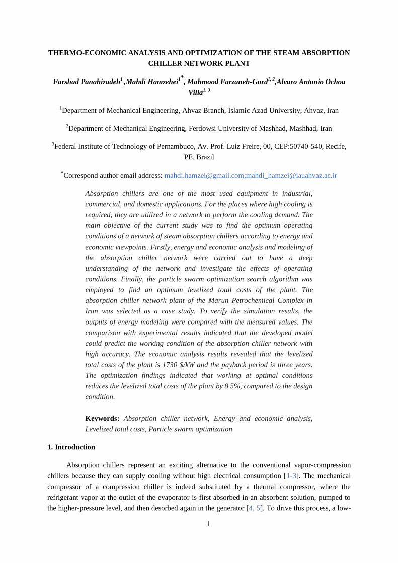
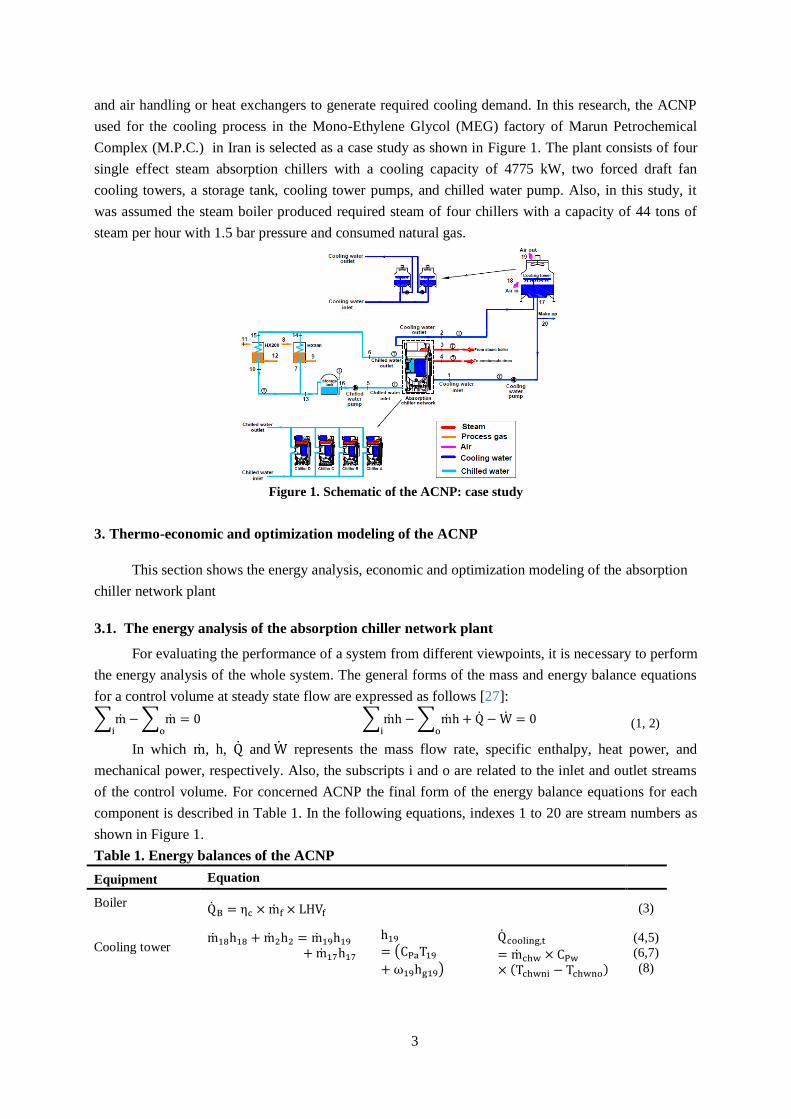
sensitivity analysis of economic indices concerning cost and income are shown in Figures 2 and 3. As
can be seen in these Figures the IRR economic index is more sensitive to change in the income and
cost of the ACNP. In the most pessimistic scenario, where the revenue is 20% lower than the
estimated value and the costs 20% higher than the initial calculation of the ACNP, the NPV and IRR
are not economically justified because the NPV is negative, but in other cases it is feasible. During the
absorption chiller network operation, changing the thermodynamic conditions of the inlet variables
such as the cooling tower water temperature, steam temperature, and chilled water temperature affect
the chillers operating parameters and LTCACNP.
Table 9. The cash flow of the ACNP
Year 0 1 2 3 5 10 20
Investment cost (FC) 3351696
Operation cost (OC) 1484000 1484000 1484000 1484000 1484000 1484000
Cash out 3351696 1484000 1484000 1484000 1484000 1484000 1484000
Annual income (AI) 0 2853760 2853760 2853760 2853760 2853760 2853760
Salvage 486882
Cash in 0 2853760 2853760 2853760 2853760 2853760 2853760
Net cash flow -3351696 1369760 1369760 1369760 1369760 1369760 1369760
Cumulative cash flow -3351696 -1981936 -612176 757584 3497104 10345904 24530386
DR 18%
NPV 3998056 $
IRR 40.8%
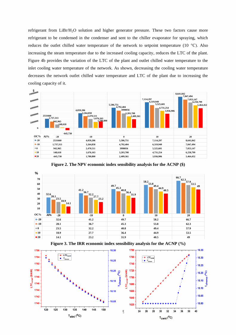
Figure 4a demonstrates the variation of the outlet chilled water temperature and LTCACNP with
network inlet steam temperature. As observed, an increase in the network inlet steam temperature
increases the heat transfer rate in the chiller’s generator and leads to the higher separation of the
9
refrigerant from LiBr/H2O solution and higher generator pressure. These two factors cause more
refrigerant to be condensed in the condenser and sent to the chiller evaporator for spraying, which
reduces the outlet chilled water temperature of the network to setpoint temperature (10 °C). Also
increasing the steam temperature due to the increased cooling capacity, reduces the LTC of the plant.
Figure 4b provides the variation of the LTC of the plant and outlet chilled water temperature to the
inlet cooling water temperature of the network. As shown, decreasing the cooling water temperature
decreases the network outlet chilled water temperature and LTC of the plant due to increasing the
cooling capacity of it.
Figure 2. The NPV economic index sensibility analysis for the ACNP ($)
Figure 3. The IRR economic index sensibility analysis for the ACNP (%)
-20 -10 0 10 20
-20 32.6 41.2 49.7 58.2 66.7
-10 28.1 36.7 45.3 53.8 62.3
0 23.5 32.2 40.8 49.4 57.9
10 18.9 27.7 36.4 44.9 53.5
20 14.1 23.2 31.9 40.5 49
32.6
41.2
49.7
58.2
66.7
28.1
36.7
45.3
53.8
62.3
23.5
32.2
40.8
49.4
57.9
18.9
27.7
36.4
44.9
53.5
14.1
23.2
31.9
40.5
49
0
10
20
30
40
50
60
70
80%
AI% OC%
-20 -10 0 10 20
-20 2531660 4,059,206 5,586,751 7,114,297 8,641,842
-10 1,737,313 3,264,858 4,792,404 6,319,949 7,847,494
0 942,965 2,470,511 3998056 5,525,601 7,053,147
10 148,618 1,676,163 3,203,708 4,731,254 6,258,799
20 -645,730 1,780,800 2,409,361 3,936,906 5,464,452
2531660
4,059,206
5,586,751
7,114,297
8,641,842
1,737,313
3,264,858
4,792,404
6,319,949
7,847,494
942,965
2,470,511
3998056
5,525,601
7,053,147
148,618
1,676,163
3,203,708
4,731,254
6,258,799
-645,730
1,780,800
2,409,361
3,936,906
5,464,452
AI%
$
OC%

10
Figure 4.a) The behavior of LTCACNP and Tchwno by changing the inlet network steam
temperature (Tchwni=16.8 °C, Tcwni=35 °C, ηSHX=0.58), b) The behavior of LTCACNP and Tchwno by
changing inlet network cooling temperature (Tchwni=16.8°C, Tstni=145 °C, ηSHX=0.58)
4.4. Optimization of the ACNP
In the present study to optimize the ACNP by PSO algorithm needs to be linked EES with
MATLABTM
and used the parameters of the PSO algorithm are shown in Table 3. This optimization is
done to minimize the LTC of the plant. The range of allowable values for decision variables and the
optimum value of those which are obtained by using the PSO algorithm are listed in Table 10.
Table 10. Range of decision variables and their optimal values in the ACNP
Decision variable Range of variation Optimal value
Steam inlet temperature (°C) 120-150 149.5
Cooling water inlet temperature (°C) 25-38 25
Chilled water outlet temperature (°C) 10-11 10
Solution heat exchanger efficiency (-) 0.5-0.7 0.7
Steam control valve opening (%) 50-100% 84
LTCACNP ($/kW) 1500-1800 1583
5. Conclusion
This study was carried out to find the optimal operating conditions of an ACNP based on energy
and economic analysis. A high accuracy computer code was developed to predict the performance of
the ACNP and investigate the effects of various parameters. To verify the developed code, the ACNP
of the Marun Petrochemical Complex was selected as a case study. The comparison between the
modeling results and experimental values showed good accuracy of the developed model. Based on
the present investigation, some conclusions can be drawn as cited below:
An increase in the ACN inlet steam temperature decreases the ACN outlet chilled water
temperature and the LTC of the plant. Reduction in the ACN inlet cooling water
temperature decreases the LTC of the plant too.
The optimization of the ACNP by using the PSO optimization algorithm shows that the
cooling water inlet temperature has a more significant effect on the LTC of the plant
rather than the steam inlet temperature. The PSO optimization algorithm results
demonstrate that working at optimal condition reduces the LTC of the plant 8.5%, rather
than design condition.
Acknowledgment
The authors express their thanks to the department of research and innovation of the M.P.C. for the
technical support in this research. The fourth author thanks the CNPq for the scholarship of
productivity nº 309154/2019-7 and the IFPE for its financial support throughout the Call
10/2019/Propesq.
References

11
[1] Ochoa, A.A.V., et al., The influence of the overall heat transfer coefficients in the dynamic
behavior of a single effect absorption chiller using the pair LiBr/H2O, Energy Conversion and
Management, 136. (2017), pp.270-282
[2] Sheykhi, M., et al., Performance investigation of a combined heat and power system with internal
and external combustion engines, Energy Conversion Management, 185. (2019), pp.291–303
[3] Ochoa, A.A.V., et al., Dynamic experimental analysis of a LiBr/H2O single effect absorption
chiller with nominal capacity of 35 kW of cooling, Acta Scientiarum Technology, 41. (2019),
pp.1-11
[4] Labus, J. M., et al., Review on absorption technology with emphasis on small capacity absorption
machines, Thermal Science, 17. (2013), pp.739-762
[5] Ochoa, A.A.V., et al., Dynamic study of a single effect absorption chiller using the pair LiBr/H2O,
Energy Conversion and Management, 108. (2016), pp.30-42
[6] Kumar, B., et al., Thermodynamic analysis of a single effect lithium bromide water absorption
system using waste heat in sugar industry, Thermal Science, 22. (2018), pp.507-517
[7] Buonomano, A., et al., A dynamic model of an innovative high-temperature solar heating and
cooling system, Thermal Science, 20. (2016), pp. 1121-33
[8] Gao, G., et al., The study of a seasonal solar CCHP system based on evacuated flat plate collectors
and organic Rankine cycle, Thermal Science, 24. (2020), pp. 915-24
[9] Panahizadeh, F., et al., Numerical study on heat and mass transfer behavior of pool boiling in
LiBr/H2O absorption chiller generator considering different tube surfaces, Thermal Science,
(2020), pp. 204-217
[10] Zhou, J., et al., Simulation analysis of performance optimization of gas-driven ammonia water
absorption heat pump, Thermal Science, 24. (2020), pp. 63-75
[11] Agboola, P., et al., Thermo-economic performance of inclined solar water distillation systems,
Thermal Science, 19. (2015), pp. S557-570
[12] Fazeli, A., et al., Thermodynamic analysis and simulation of a new combined power and
refrigeration cycle using artificial neural network, Thermal Science, 15. (2011), pp. 29-41
[13] Mohammadi, Z., et al., Advanced exergy analysis of recompression supercritical CO2 cycle,
Energy, 178. (2019), pp. 1-12
[14] Alcantara, S.C.S., et al., Natural gas based trigeneration system proposal to an ice cream factory:
An energetic and economic assessment. Energy Conversion and Management, 197. (2019),
pp.111860
[15] Mancic, M.V., et al., Techno-economic optimization of configuration and capacity of a
polygeneration system for the energy demands of a public swimming pool building, Thermal
Science, 22. (2018), pp. S1535-S1549
[16] Silva, H.C.N., et al., Modeling and simulation of cogeneration systems for buildings on a
university campus in north east Brazil – a case study, Energy Conversion and Management, 186.
(2019), pp.334-348

12
[17] Ochoa, A.A.V., et al., Techno-economic and exergoeconomic analysis of a micro cogeneration
system for a residential use, Acta Scientiarum Technology, 38. (2016), pp. 327-338
[18] Cardoso, J., et al., Techno-economic analysis of olive pomace gasification for cogeneration
applications in small facilities, Thermal Science, 23. (2019), pp. S1487-1498
[19] Souza, R.J., et al., Proposal and 3E (energy, exergy, and exergoeconomic) assessment of a
cogeneration system using an organic Rankine cycle and an absorption refrigeration system in the
north east Brazil: Thermodynamic investigation of a facility case study, Energy conversion and
Management, 217. (2020), pp.113002
[20] Ebrahimi-Moghadam, A., et al., Proposal and assessment of a novel combined heat and power
system: energy, exergy, environmental and economic analysis, Energy Conversion and
Management, 204. (2020), pp.112307
[21] Ebrahimi-Moghadam, A., et al., Comprehensive techno-economic and environmental sensitivity
analysis and multi-objective optimization of a novel heat and power system for natural gas city
gate stations, Journal of Cleaner Production, 262. (2020), pp.121261
[22] Mancic, M.V., et al., Optimization of a polygeneration system for energy demands of a livestock
farm, Thermal Science, 20. (2016), pp. S1285-S1300
[23] P. Zadeh, M., Thermo-economic-environmental optimization of a micro turbine using genetic
algorithm, Thermal Science, 19. (2015), pp. 475-487
[24] Shamoushaki, M., Exergy, economic and environmental (3E) analysis of a gas turbine power
plant and optimization by MOPSO algorithm, Thermal Science, 22. (2018), pp. 2641-2651
[25] Yang, Y., et al., Optimal design of distributed energy resource systems under large-scale
uncertainties in energy demands based on decision making theory, Thermal Science, 23. (2019),
pp. 873-882
[26] Panahizadeh, F., et al., Energy, exergy, economic analysis and optimization of single‑ effect
absorption chiller network, Journal of Thermal Analysis and Calorimetry, 140. (2020), pp. 1-31
[27] D.Vuckovic, G., et al., Avoidable and unavoidable exergy destruction and exergoeconomic
evaluation of the thermal processes in a real industrial plant, Thermal Science, 16. (2012), pp.
S433-446
[28] Wall, G., Optimization of refrigeration machinery, International journal of refrigeration, (1991),
pp. 1-14
[29] Packman boiler manufactory, Iran, Esfahan, http://www.packmangroup.com
[30] Iran natural gas price, URL: http://mgd.nigc.ir/
[31] Iranian central bank. URL: http://www.cbi.ir/
[32] Monoethylene glycol (MEG) price. URL: https://www.eranico.com
[33] Noorpoor, A.R. and Nazari kudahi, S., CO2 emissions from Iran’s power sector and analysis of
the influencing factors using the stochastic impacts by regression on population, affluence and
technology (STIRPAT) model, Carbon Management, (2015), pp. 101-116

13
[34] Jannatabadi, M., et al., District cooling systems in Iranian energy matrix, a techno-economic
analysis of a reliable solution for a serious challenge, Energy, 214. (2020), pp. 1-13
[35] Fabricius, M., et al., Utilization of excess production of waste fired CHP plants for district
cooling supply, an effective solution for a serious challenge, Energies, 13. (2020), pp. 1-20
[36] Bhatia, A., Overview of vapor absorption cooling systems course no: M04-025
Paper submitted: 19.06.2020
Paper revised: 05.12.2020
Paper accepted: 10.12.2020