1

gr-qc/9410015

Thermodynamics of a black hole in a cavity

Renaud Parentani1x, Joseph Katz2y and Isao Okamoto2

1 The Racah Institute of Physics, The Hebrew University of Jerusalem, Jerusalem91904, Israel2 Division of Theoretical Astrophysics, National Astronomical Observatory, Mizusawa,Iwate 023, Japan (E-mail: okamoto@gprx.miz.nao.ac.jp)

Abstract. We present a uni�ed thermodynamical description of the con�gurations consisting onself-gravitating radiation with or without a black hole. We compute the thermal uctuations andevaluate where will they induce a transition from metastable con�gurations towards stable ones.We show that the probability of �nding such a transition is exponentially small. This indicates that,in a sequence of quasi equilibrium con�gurations, the system will remain in the metastable statestill it approaches very closely the critical point beyond which no metastable con�guration exists.Near that point, we relate the divergence of the local temperature uctuations to the approachof the instability of the whole system, thereby generalizing the usual uctuations analysis in thecases where long range forces are present. When angular momentum is added to the cavity, theabove picture is slightly modi�ed. Nevertheless, at high angular momentum, the black hole losesmost of its mass before it reaches the critical point at which it evaporates completely.

xPresent address: Laboratoire de Physique Theorique de l' Ecole Normale Superieure, 24 Rue Lhomond, 75005 Paris,France (E-mail: parenta@physique.ens.fr)

yPermanent address: The Racah Institute of Physics, Jerusalem 91904, Israel (E-mail: jkatz@hujivms.bitnet)

2

1. Introduction and summary

A black hole in an isolated cavity which is bigger than its Schwarzschild radius can be in equilibrium

with surrounding radiation only if the total energy E of the system is greater than a critical value EC,

which depends on the volume of the cavity and the number of �elds in the radiation (Hawking 1976).

While local equilibrium con�gurations exist for energies greater than EC, it is generally assumed that

black holes must evaporate if EC < E < EB ' 1:3EC since for E < EB pure radiation has more

entropy than the composite system (Gibbons and Perry 1978).

This holds only if the system is given unlimited time to relax. If one considers instead a sequence of

con�gurations starting, say, from an equilibrium at E = EB and in which the total energy is decreased

quasi-statically, the system reaches new local equilibrium con�gurations in a �nite time (Zurek 1980).

During that time, the probability of �nding a uctuation high enough that the black hole completely

evaporates is exponentially small. So small that the black hole is most likely to survive in a metastable

superheated state up to energies very close indeed to EC (Okamoto, Katz and Parentani 1994). This

is true for cavities whose radius L� is greater than 106 Planck lengths lP = (�hG=c3)1=2 � 10�33cm

(L � L�=lP > 106). For those cavities, back-reaction due to quantum matter e�ects (York 1985),

quantum gravity and spontaneous nucleation due to thermal uctuations (Piran and Wald 1982)

may be neglected since the maximum temperature, reached by equilibrium con�gurations, is always

smaller than TD ' 0:37L�1=2� (in Planck units). Thus more than three orders of magnitude separate

the equilibrium temperature from the Planck one. This indicates that a thermodynamic analysis may

be safely performed. On the contrary, for smaller boxes the validity of this analysis becomes dubious.

Self-gravitating thermal radiation exhibits a similar behavior in an evolutionary sequence in which

the total energy increases quasi-statically. Indeed, there is now an upper limit of energy EA ' 0:25L

(here E is measured in Planck units) above which no equilibrium con�guration exists (Klein 1947).

Thus for energies EB < E < EA (EB ' 0:20L3=5 � EA ' 0:25L for L > 106) pure radiation is in

metastable superheated states. We shall prove that, as in the black hole situation, pure radiation is

�Throughout the text numerical values are given with two signi�cant digits

3

most likely to remain in those metastable states almost up to EA. At that point, a thermodynamic

as well as dynamical instability (Sorkin, Wald and Zhang 1980) develops and most of the radiation

collapses into a black hole leading to a composite state of a black hole in equilibrium with surrounding

left-over radiation. The spontaneous evaporation of the black hole into pure radiation near EC and

the collapse of the radiation near EA provides thus a uni�ed picture relating the di�erent phases of a

black hole and self-gravitating radiation in a cavity.

Uniform rotation added to the cavity gives a total angular momentum J shared between the

radiation and the black hole. The equilibrium con�gurations change in the following way. The critical

energy EC(J) at which the black hole evaporates is now a function of J . It increases with increasing

angular momentum while the fraction of black hole energy at that point EbhC=EC decreases from 4=5

at J = 0 to almost zero in the limiting rotating case: J = L2=2. Hence for fast rotating cavities,

at �xed J and with slowly decreasing total energy, superheated Kerr black holes will evaporate with

little latent heat, since black holes survive almost down to the critical point EC(J).

All of this concerns microcanonical situations in which the total energy is the control parameter.

In canonical situations, with the temperature kept �xed, almost all the con�gurations wherein a black

hole coexists with radiation are unstable. There exits nevertheless a narrow range of energies for very

fast rotating cavities in which the canonical ensemble is stable. One thus recovers in this narrow range

the already noticed ip of the heat capacity for Kerr black holes (Davies 1981, Kaburaki et al. 1993;

cf. Katz et al. 1993 for Kerr-Newman black holes). When the radiation is included, this happens,

however, when gravitational e�ects (neglected in the present analysis) are important.

In this paper, we analyze the stability limits, the di�erent degrees of instability and the uctuations

of each of the two states of the system (with or without black hole) in evolutionary sequences of equi-

librium con�gurations, with and without angular momentum. The analysis is purely thermodynamic.

We assume there exists a state function whose stationary value is a function of the total mass-energy

E, total angular momentum J and the volume of the cavity V = �L3. We consider separately the mi-

crocanonical and the canonical ensembles since they are not equivalent. In a microcanonical ensemble,

4

E is the main control parameter and the inverse temperature

1

kT=@(S=k)

@E= �(E; J; L) (1)

is the conjugate parameter of E with respect to the total entropy S. In a canonical ensemble, the

Massieu function is not S but S=k� �E = ��F (F is the free energy), the main control parameter is

� and the conjugate parameter of � with respect to ��F is

@(��F )@�

= �E(�; J; L): (2)

The linear series of equilibrium con�gurations in both ensembles, �(E) and �E(�) at �xed J and L,

are identical but the stability limits are not. Stability limits are obtained by applying the Poincar�e

method to linear series (see Ledoux 1958). We shall consider the linear series of conjugate parameters

(Katz 1978, 1979; Thompson 1979) since this is the most appropriate way to observe changes of

stability.

While state functions out of equilibrium, , are never used, some assumptions must be made

about which are stated in section 2 where the extremization of the entropy is related to the Einstein

equations when self-gravity is taken into account. Stability analysis in terms of Poincar�e's method is

then brie y reviewed. We shall see that we need to know �(E) only and not itself, a useful feature

when analyzing the stability of self-bound radiation in a box. Furthermore, having determined �(E)

from the solution of the Einstein equations, we do not need to attribute a priori an entropy to the

black hole. Instead, we recover it from the equilibrium con�gurations.

The theory of uctuations is then considered. Fluctuation theory as given by Landau and Lifshitz

(1980) and Callen (1985) is not entirely applicable to self-gravitating systems for the reason that when

gravitational interactions are important one cannot anymore split the system into a little subsystem

and the rest which behaves like a heat reservoir for the little one. Nevertheless, we shall see that the

mean quadratic uctuations of the inverse temperature, in a small subsystem, are simply related to

its own thermodynamic parameters as well as the parameters of the whole system.

Section 4 gives details about �(E) in non-rotating and rotating cavities. Fluctuations near turning

points are calculated in section 5 and a summary of stability conditions and phase transitions in slowly

5

evolving systems through a succession of quasi-equilibrium states is described in section 6.

2. The stability of equilibrium con�gurations in mean �eld theory

In a stationary axially symmetric distribution of matter in local thermodynamic equilibrium, with

�xed total mass-energy and angular momentum, and with Einstein constraint equations given, the

total entropy S is stationary, �S = 0, if Einstein \dynamical" equations are satis�ed. Then Tolman's

(1934) thermodynamic equilibrium conditions for local temperature hold and the angular velocity is

uniform [Katz and Manor (1975); for non-rotating, spherical con�gurations see Cocke (1965)]. Here

we shall use the partition function (Hawking 1978, Horwitz and Weil 1982, York 1988 and Brown

et al. 1990) to sketch a formal deduction of both equilibrium and stability conditions for spherical

distributions with zero angular momentum. This procedure will naturally exhibit the relations between

the Einstein equations, quantum �eld theory in curved space and the extremization of the entropy.

Consider, for de�niteness, the state function which encodes the total number of states of a scalar

�eld in a curved spacetime with total mass-energy E as measured from in�nity. The �eld is con�ned

to a spherical box of \radius" L (i. e. the surface of the cavity is 4�L2). Then (E;L) is

(E;L) = eS(E;L) = Tr�(E �H) =

Zdt

2�eiEt

Z Dg��DiffD� exp [iSEin+ iS�] : (3)

The denominator \Diff" indicates that one should not integrate over geometries related by a di�eo-

morphism; SEin =Rd4x

p�gR, and S� =Rd4x

p�gg��@��@��. Since there is no unique de�nition of

a local matter Hamiltonian in general relativity, we have used the path integral formalism. We refer to

Regge and Teitelboim (1974) for a de�nition of energy in asymptotically at spacetimes. Integrating

in (3) over all periodic matter con�gurations (of period t), one obtains

(E;L) =

Zdt

2�

Z Dg��Diff exp [iEt+ iSEin] Z[fg��g; it] (4)

where Z is the partition function at �xed Lorentzian time t in the background geometry fg��g.

Calculating (4) at the stationary con�guration of iEt+ iSEin + lnZ[fg��g; it] gives the dominant

contribution to . At the stationary point, g�� satis�es the time independent Einstein equations with

6

an energy tensor of a thermal bath if at the saddle point t = �i�. In the absence of horizons, the matter

�eld con�gurations are de�ned for 0 � r � L and one recovers, up to quantum matter corrections, the

equations of a self-gravitating perfect uid (Klein 1947, Gibbons and Hawking 1978). In the presence

of horizons (see Carlip and Teitelboim 1993 for the treatment of the boundary term at the horizon),

the regularity of the stress energy-momentum tensor, needed to satisfy Einstein equations, �xes the

temperature of the matter (Hawking 1978). Then by integrating the time-time Einstein constraint

equation one obtains

m(r;Mbh) =Mbh + 4�Z r

2Mbh

dr0r02hT tt (r

0)iHH;Mbh(5)

where hT tt iHH;Mbh

is the expectation value of the energy density, outside a black hole of mass Mbh, in

the Hartle-Hawking vacuum (Howard 1984). Since E = m(L;Mbh), one may invert this relation and

express Mbh in terms of E and L. Therefore, one obtains the sought-for � = �(E) law (with L held

�xed). Notice that Einstein equations with back-reaction taken into account provide an alternative

way to determine the entropy of the black hole. Indeed, by integrating �(E)dE one obtains the total

entropy S(E;L), which reduces to the black hole entropy when the radiation energy is negligible.

One may also subtract from S(E;L) the entropy of the radiation, but there is an arbitrariness in this

subtraction | since there is no unique de�nition of the entropy density nearby the hole where the

Tolman relation breaks down|which indicates that the concept of the entropy of an isolated black

hole is probably meaningless.

In order to illustrate the Poincar�e method, we perform the t-integration in (4) (Horwitz and Katz

1978) which gives an of the form

(E;L) =

Z Dg��Diff e

�w(E;L;fg��g): (6)

We do not need to be speci�c about the function w(E;L; fg��g) precisely because Poincar�e analysis

deals with the succession of extrema of w(E;L; fg��g) and not the function itself. A speci�c example

is given in Sorkin et al. (1980) in the case of pure radiation without horizon, wherein w depends on

grr only.

7

The stationary value of w is the classical equilibrium entropy S. The local stability of equilibrium

con�gurations is controlled by the quadratic uctuations of w. Imagine we make a Fourier decompo-

sition of the g�� 's. Since the domain of existence is �nite (0 � r � L), the g��'s are replaced by a

denumerable set of variables, say, xi (i = 1; 2; ::::). To order two, w may thus be written

w � S +1

2

�@2w

@xi@xj

�e

(xi �X i)(xj �Xj) (7)

where an index e means `at equilibrium' [thus S = we] and X i(E;L) are equilibrium values of xi.

Let �i's denote the (ordered: �1 � �2 � :::) elements of the diagonalized matrix �(@2w=@xi@xj).

The �i's are known as the Poincar�e coe�cients of stability (Lyttleton 1953). The equilibrium is

thermodynamically (locally) stable, or stable for arbitrary small uctuations, if and only if all the �i's

are positive i. e. if �1 > 0. In unstable situations, the number of �i < 0 characterize the degree of

instability.

The matrix �(@2w=@xi@xj)e is a second order di�erential operator of dimension one over a �nite

domain. We may assume that the spectrum of eigenvalues is non-degenerate: �1 < �2 < ::: . Indeed,

the slightest asymetric perturbation in a system would lift the degeneracy (Thompson and Hut 1973).

Having then a non-degenerate spectrum of Poincar�e coe�cients, the following properties hold (Katz

1978, 1979):

(a) Consider the linear series �(E). Changes of stability along the linear series can only occur at ver-

tical tangents, @�=@E = �1, like point A or C in �gure 1. Such points where E is locally minimum

or maximum are called turning points. Between two vertical tangents all equilibrium con�gurations

have the same degree of instability.

(b) In the neighborhood of a vertical tangent, when the linear series turns clockwise (its tangent goes

from negative to positive values through in�nity), one Poincar�e coe�cient changes sign from nega-

tive to positive value. That is, the system becomes stable or less unstable. If the linear series turns

counter-clockwise, the changes of sign are reversed and the system becomes unstable or more unstable.

It is thus enough to know the degree of stability of one con�guration to know the degree of stability

of all con�gurations.

8

(c) Of particular interest are linear series with multiple turning points spiraling inwards against the

clock. If we follow the spiral towards the limit point, we meet a succession of vertical tangents and

beyond each one, an additional Poincar�e coe�cient becomes negative. Counter-clockwise spirals rep-

resent thus a succession of equilibrium con�gurations that are more and more unstable.

Upon considering di�erent ensembles, the following properties hold (Parentani 1994):

(d) The most stable ensemble is always the most isolated one. The degree of stability of equilibrium

con�gurations in any ensemble related by a Legendre transformation (which expresses the contact

with a reservoir) to the most stable is immediately known if one knows the degree of stability in the

most stable ensemble.

3. Fluctuations in gravitating systems

In classical thermodynamics, it is well known (Landau and Lifshitz 1980 (x112), Callen 1985 and

Landsberg 1990) that the mean square uctuations of the fundamental thermodynamic quantities

pertaining to any small part of a system (or to the system as a whole) are related to the speci�c heat.

For instance, in a canonical ensemble of total volume V , the mean quadratic uctuations (�E)2 of

the energy E induced by the contact with the reservoir are given by

(�E)2 =@(�E)@�

=CV

�2 (8)

where CV is the heat capacity at constant volume V . The mean square uctuations (��)2 of the

inverse temperature which result from those energy uctuations are given by

(��)2 = � @�

@E=

�2

CV

: (9)

since � is a function of E only.

In a microcanonical ensemble, these uctuations vanish since the total energy E is kept �xed.

Nevertheless, within a small subsystem of volume V 0, the temperature uctuates and the mean square

uctuations of �0 are given by

(��0)2 = � @�0

@E0=

�02

CV 0

: (10)

9

where CV 0 is the speci�c heat of the subsystem and E0 its energy. This equation is valid only if the

speci�c heat of the rest of the system is much bigger that the one of the subsystem (for homogeneous

systems it requires V 0 � V ). The equivalence of ensembles (the equality of the uctuations (10)

whether one works in the microcanonical or the canonical ensemble) means therefore that the rest of

the system can be correctly treated as a heat reservoir for the little subsystem. Finally, we recall that

the 'true' uctuations are given by these estimates only if the characteristic dynamical time for the

uctuations to evolve is much bigger than � itself.

In gravitating systems, there are long range forces. Therefore, when gravitational interactions are

important, one cannot treat the rest of the system as a passive reservoir. Indeed the existence of stable

microcanonical ensembles with negative speci�c heat indicates the decisive role of the energy constraint

between the little subsystem and the rest. Furthermore, we stress the fact that when a microcanonical

ensemble approaches instability, its heat capacity given in equation (8) is always negative (thus the

canonical ensemble is already unstable) for stable states and positive in unstable states (for which the

canonical ensemble is still unstable) see section 4 and, for instance, �gure 1.

The relation between mean square uctuations and thermodynamic coe�cients in gravitating

systems is thus more complicated than equation (10) and we shall display it in two steps. We shall

�rst see that, since the vicinity of a turning point is dominated by a single eigenmode, one can relate

the uctuations of the least stable mode x1 to the heat capacity of the whole system CV . Then, we

shall relate the uctuations of the inverse temperature within a small subsystem to CV itself. To prove

the �rst point, consider a microcanonical ensemble (with J = 0) in which we de�ne a temperature

function ~�(xi;E; V ) away from equilibrium (see also Okamoto et al. 1994)

~� =@w

@E: (11)

At equilibrium one has ~�(X i(E; V );E; V ) = �(E; V ) where the equilibrium values xi = X i(E; V ) are

solutions of

@w

@xi= 0: (12)

10

Therefore, the slope of the linear series and the derivatives of ~� are related by

@�(E; V )

@E=

@~�(xi;E; V )

@E

!e

+Xi

@~�

@xi

!e

@X i(E; V )

@E(13)

The derivative @X i=@E can be obtained from equation (12) by the following identity

�@

@E

��@w

@xi

�e

��=

@~�

@xi

!e

� �i@X i

@E� 0 (14)

where there is no summation on i. Thus, from equation (14) we deduce @X i=@E in terms of (@~�=@xi)e

which we may insert into (13) to obtain

@�

@E=

@~�

@E

!e

+Xi

(@~�=@xi)2e�i

: (15)

Consider now a linear series of stable con�gurations near a turning point. At that point the �rst

eigenvalue �1 changes sign. As a result the right hand side of equation (15) is entirely dominated by

the �rst term

@�

@E' 1

�1

@~�

@x1

!2

e

: (16)

The changes of w are also dominated by the uctuations of x1 and given by

w ' S � 1

2�1(�x

1)2 (17)

which, with equation (16), becomes

w ' S � 1

2

(�~�)2

@�=@E(18)

where

�~� =

@~�

@x1

!e

�x1: (19)

This �~� represents uctuations in the inverse-temperature function induced, near the critical point,

by the uctuations of the least stable mode x1. We can now use the standard arguments of uctuation

theory (Landau and Lifshitz 1980) and say that the probability dW for a uctuation of ~� in the range

~� +�~� and ~� + �~� + d~� is proportional to exp(w � S) and therefore,

dW =1p2�

d~�p(@�=@E)

exp

"�1

2

(�~�)2

(@�=@E)

#(20)

11

Thus the mean square uctuations of ~� are given by

(�~�)2 =@�

@E= � �2

CV

: (21)

They are bounded when the microcanonical ensemble is stable (i. e. when �1 > 0 or as we already

point out when CV < 0. See equation (16)). It is convenient to express dW in terms of CV and of the

dimensionless ratio

~�(xi;E;L)

�� ~u: (22)

Then

dW =

s�CV

2�exp

�+1

2CV (�~u)2

�d~u (23)

and, following (21) the mean square uctuations of ~u are

(�~u)2 = �C�1V : (24)

Our task now is to relate those rather formal uctuations of ~� to the uctuations of the temperature

within a small part of the system as well as to understand the origin of the unusual sign in equation

(21). As we have already said, in the presence of long range forces, one cannot exactly split a system

into two parts since there is no more a local de�nition of energy. If nevertheless some small part is

less coupled gravitationally to the rest of the system, one may use it as the "small" system in which

one can compute the uctuations of �. When this is not the case, we shall see that one can still

consider the uctuations within the outermost layer of radiation even though the energy into that

layer is not well de�ned. We designate by the subscript 2 the little subsystem which is con�ned for

radii L � l < r < L (where l � L). The subscript 1 refers to the rest of the system which is thus

either the black hole surrounded by radiation up to that last layer, or pure radiation. Instead of the

energy, we shall use the Schwarzschild mass (since it is a local quantity) and we thus split it into E1

and E � E1. We shall see that the partition mass E1 will play a role very similar to the least stable

mode x1. This is because @x1E1 6= 0.

12

Let w(E1;E; V ) be the entropy out of equilibrium by which we now mean that the only variable

out of equilibrium is E1. All other variables have been replaced by their equilibrium values. Then

w(E1;E; V ) = S1(E1; V1) + S2(E �E1; V � V1;E1) (25)

where S1 and S2 are the entropies of the two parts. We emphasize the double dependence of E1 in S2.

When E1 varies, the mass left over in the system 2 is E�E1 but the gravitational potential in which 2

evolves is changed as well. This later dependence is nevertheless parametric if l � L. By parametric

we mean that upon taking derivatives with respect to E1, this later dependence gives an additional

term which is O(l=L) smaller than the usual term and which may be safely neglected. Equilibrium

between the two parts requires, as usual, the equality of the temperatures:

@E1w(E1;E; V ) = @E1

S1 + @E1S2 � �1 � �2 = 0 (26)

where �1 and �2 are the inverse temperatures of the two parts and where we have neglected the

additional term (This does not mean that we neglect completely the extra dependence in E1, for

instance, �2 depends explicitly on E1 trough the Tolman dependence (see the Appendix equation

(A.3))). Then the lowest order variations of w near equilibrium due to an exchange of energy �E1 is:

w � S =1

2(@2E1

w)(�E1)2 =

1

2[@E1

�1 + @E2�2] (�E2)

2 (27)

This energy uctuation induces, in turn, a uctuation of �2 in the small part given by

��2 = �E2(@E2�2) (28)

Then the entropy uctuation induced by the latter one is

w � S =1

2(@�

2

E2)h1 + (@E1

�1)(@�2

E2)i(��2)

2 =1

2(@�

2

E2)dE

d�(@E1

�1)(��2)2 (29)

since the slope of the �(E) curve of the entire system is given by

d�

dE= (@E2

�2)

�1� dE1

dE

�= (@E1

�1)h1 + (@E1

�1)@�2

E2

i�1

(30)

because

dE = dE1

h1 + (@�

2

E2)(@E1�1)i

(31)

13

Thus the mean square uctuations of �2 given by the inverse coe�cient appearing in equation (29)

are

(��2)2 = �(@E2

�2)d�

dE(@�

1

E1): (32)

This is the generalisation of equation (10) when one cannot treat the rest of the system as a passive

reservoir. Indeed, one does recover (10) when the subsystem 1 can be approximated by the whole

system in which case the coe�cient of @E2�2 is 1. One sees also that the point wherein the uctuations

of �2 will diverge is controlled entirely by the divergence of d�=dE when the denominator in equation

(30) vanishes. That is, one probes locally, through the uctuations in the small subsystem the stability

of the whole system 1+ 2. Furthermore, near the critical point, the mean uctuations of �2 are equal

to the uctuations of ~� (and therefore independent of l) since (@�2

E2)(@E1�1) = �1 at the critical

point as seen in equation (30). This later factor of �1 explains the unusual sign in equation (21).

For the interested reader, we also point out the analogy of equation (32) which gives the uctuations

when the rest of the system cannot be treated as a reservoir and the expression which relates the

uctuations in one ensemble to the uctuations in another ensemble related to the �rst one by a

Legendre transformation (Parentani 1994). In both cases when the ensembles are nonequivalent, the

uctuations are controlled by the correction factor: d�dE(@�

1

E1), the coe�cient of @E2�2 in equation

(32). And it is only when the ensembles are equivalent that this factor reduces to 1. Another common

feature is the fact that when d�=dE = 0 it does not imply that the uctuations of �2 vanishes because

@E1�1 vanishes as well, see equation (30).

For a canonical ensemble, when one consider con�gurations which are stable microcanonically, the

necessary and su�cient condition for stability is the positivity of CV . For those con�gurations only

one may safely apply the analysis of Landau and Lifshitz and �nd that the uctuations of the total

energy are indeed given by equation (8). Finally let us mention that equivalent ensembles would have

vertical and horizontal slopes in �(E) at practically the same point since both ensembles become

simultaneously unstable. Thus the curve �(E) would make an angle bigger than 90�. Nothing like

that is happening in the following situations.

14

4. The linear series of conjugate parameters

In Planck units, E, J and � are respectively given by

E =E�

EP

; J =J�

�h; � = ��EP (33)

in which EP =p�hc5=G � 1016erg and asterisks denote quantities in cgs units. Instead of using Planck

units for E, J and �, we shall use dimentionless quantities expressed in terms of G, c and L� as is

common in classical general relativity. One thus de�ne

E =GE�

c4L�; J =

GJ�

c3L�2; b =

�hc��

8�L�: (34)

Then E varies between 0 and 1=2 (the Schwarzschild limit) and since J� < E�L�=c (the centrifugal

limit), J is always smaller than E . Thus,

0 � J � E � 1

2: (35)

We shall see nevertheless the appearance of a fourth dimensionless quantity L = L�=lP which will

re ect the fact that the Hawking temperature has a quantum origin. Finally, the relation between E,

J , � and E , J , b is

E =E

L; J =

J

L2; b =

�

8�L(36)

(i) Schwarzschild Black Holes.

Consider �rst a Schwarzschild black hole of mass M�bh in equilibrium with radiation enclosed in a

spherical cavity with �xed radius L. At su�ciently low temperature (high � or b), when most of the

mass-energy is in the black hole, the total energy of the black hole and the radiation is, to a good

approximation (see the Appendix) given by the sum of mass-energies as in at spacetime (Hawking

1976); in Planck units

E = Ebh +Erad =�

8�+�2

15nV ��4 (37)

15

where n is the sum over the helicity states of the massless �elds. Translated into our classical units,

(37) becomes

E = Ebh + Erad = b+ �L�2b�4; � =4�3

45

�1

8�

�4

n ' 6:91 � 10�6n: (38)

From now on we shall take n = 1. The function E(b) becomes eventful when Ebh and Erad are of the

same order of magnitude. Indeed the lower bound for E is reached when

dEdb

= 0 (39)

at which point (C in �gure 1a) one has

Ebh = 4Erad; E = EC =5

4bC; bC = (4�L�2)

1

5 = 0:123L�2

5 : (40)

When E > EC , the system's energy is dominated either by the black hole or by the radiation.

Indeed for b > bC, when E > 1:6EC, less than 1% of the energy is in the radiation. For b < bC,

when E > 25EC , less than 1% is in the black hole mass. At higher energies, along this later series,

when b � L�1=2, one has to take into account the radiation self-gravitating e�ects and solve Einstein

equations [Klein (1947) in the case of pure radiation, see also the Appendix]. One �nds that there is a

maximal temperature where bD ' 0:11L�1=2 and ED ' 0:123 (see �gure 1b). For still higher energies,

b increases again till one �nds a maximal energy EA ' 0:246 where bA ' 0:135L�1=2 beyond which the

are no more equilibrium con�gurations.

Both curves, b(E) and b(Erad) are drawn in �gure 1a and 1b. In �gure 1b the two lines are

almost on top of each other for E >� ED (due to the small mass of the hole: Ebh=Erad � b � L�1=2)

and they spiral inwards counterclockwise with an almost common limit point Z at EZ = 3=14 and

bZ ' 1:23bD ' 0:132L�1=2.

Such counterclockwise spirals appear in Newtonian theory as well as in general relativity for equa-

tions of state of the form P = K� where P is the pressure, � the density and K a number (Chan-

drasekhar 1972); here K = 1=3. The inward spiral will not di�er very much whether we keep L or the

proper volume of the sphere �xed. Therefore, stability limits will not di�er signi�cantly either.

16

The two linear series b(E) and b(Erad) coexist between two vertical lines for EC � E � EA. Thus

between these lines there will be always one metastable state. We emphasis the origin of EC < EAwhich is due to the di�erent nature of the instability: with or without a black hole at the Hawking

temperature. This leads to the scaling

EC

EA

= 0:65L�2=5: (41)

Very important also is the fact that there is a maximal temperature TD ' 0:37L�1=2. Thus for

L > 106, T is always at least three orders of magnitude below the Planck temperature. We may

thus safely neglect quantum matter e�ects (York 1985), quantum gravity and spontaneous nucleation

(Piran and Wald 1984). For smaller boxes, not only should one take into account the quantum

matter e�ects induced by the presence of the hot black hole, but one has presumably to abandon the

thermodynamic analysis all together since the uctuations become important and are not governed

anymore by their thermodynamics estimates. Indeed, for those con�gurations, the thermal and the

dynamical characteristic times come to coincide.

Finally, we mention that Balbinot and Barletta (1988) computed the change of the black hole

entropy Sbh due to some quantum matter back-reaction. This provides a model for black hole remnants

since the tiny black hole may now be in equilibrium with radiation for arbitrary large (or small)

temperatures. One easily shows that for cavities with L > 106 one �nds the linear series to be

almost unmodi�ed and thus stability limits una�ected (contrary to what was suggested) since the

modi�cations are dimensionalized by the Planck mass and since T <� 0:37 10�3.

(ii) Rotating Black Holes.

Consider now a Kerr black hole at mid-height on the z axis of a cylindrical cavity of radius L�.

When thermodynamical equilibrium is achieved, the radiation has the same temperature as the hole

and rotates with the same angular velocity: bh = rad. The peripheral velocity of the cavity, in units

of c, is

� =radL

�

c; 0 � � � 1: (42)

17

Schumacher et al. (1992) have calculated what becomes of equation (38) when the gravitational pull

of the hole and the self-gravitational e�ects of the radiation are neglected. This amounts to add to the

energy of a rotating black hole Ebh(b; �) the energy of the radiation calculated (in special relativity)

in rotating coordinates. We shall push the analysis of that approximation beyond its presumed limits

of validity in order to gain some insight of what may still happen at very high angular momentum

(� ! 1) when general relativity has to be taken into account.

Introducing a non-dimensional parameter h � J=MbhrH where rH is the radius of the horizon

(Okamoto and Kaburaki 1992), the mass-energy, the angular momentum and the angular velocity of

the hole can be written

Ebh = b(1� h2); Jbh = 2h

1 + h2(1� h2)2b2; 0 � h � 1 (43)

bh =4�

�

h

1� h2: (44)

At equilibrium, bh = cav, thus equations (42) and (44) give

�(h; b) =1

2b

h

1� h2: (45)

For a cylinder of height H� = 2L�, Schumacher et al. found

E(b; h) = b(1� h2) +3

2�L�2b�4 1� �2=3

(1� �2)2(46)

and

J (b; h) =2h

1 + h2(1� h2)2b2 + �L�2b�4 �

(1� �2)2: (47)

Equations (47) with (45) immediately indicate that most of the angular momentum is in the radiation

except when b is close to 1=2, i. e. when the black hole �ll up the entire cavity. For a given value of Jheld �xed, equation (47) gives h(b) which, substituted in equation (46) gives b(E). The b(E) function

can only be written in parametric form and we have to solve it numerically. We have drawn b(E) for

J = 1=40 in �gure 2a and for 1=8 in �gure 2b.

A common feature of the two linear series of �gures 1 and 2 is that black holes and radiation coexist

to the right hand side of a vertical line CCrad since there is always a minimum energy EC(J ) required

18

to �nd a black hole in equilibrium with the radiation. There is no maximal energy, the equivalent

of EA, on the right hand side because we have not take into account the self-gravity of the rotating

radiation. There are also two important modi�cations in the behavior of b(E) at �xed J when one

compares linear series at di�erent J . Both are shown in �gure 3. First, the turning point C moves

in the plane (E ; b); EC increases with J . Second, the energy of the black hole at C, EbhC(J )| the

energy gained by the radiation between C and Crad|divided by the total energy EC(J ) decreaseswith J .

Another novelty appears for J >� 1=40. We remind the reader that in the absence of radiation,

it was noted that for Jbh=M2bh>� 0:68 the slope @�=@Mbh becomes negative, going through 0 (Davies

1977). When the radiation is taken into account, there is no change of sign in @�=@E since the radia-

tion dominates the equilibrium con�guration before one approaches the critical ratio 0:68 of Jbh=M2bh.

For J >� 1=40 y one does recover this phenomenon in a small interval of energy (see �gure 2b). There

are now two changes of sign upon decreasing the energy, before the black hole starts to evaporate. At

lower energies the radiation dominates the equilibrium again and @�=@E returns positive.

5. Fluctuations near the turning points

We shall now compute the mean square uctuations of the rescaled variable ~u, equation (32), near the

turning points C and A. We shall also �nd the probabilities dW , equation (23), that the uctuations

be big enough for the system to jump from metastable to stable con�gurations. Finally we shall say

a few words about characteristic times and for the probability rates.

At the turning point CV = 0. Thus, for an equilibrium con�guration P in the vicinity of the

turning point, to lowest order in (�P � �0) where �0 stands for either �C or �A one has

�CV = �2P

�@E

@�

�P

' �20

�@2E

@�2

�0

(�P � �0) =

��3 @

2E

@�2

�0

�u (48)

yThis limit is obtained by substituting � from (45) into (47). For a given J , one �nds 3 values of 0 � h � 1corresponding to 3 points on b(E). Two of the points are on the left and right of the local maximum, point X in �gure2b, when J is high enough, say 1=8. As J decreases the 2 points come closer to each other and point X goes down theline b(Ebh). At about J ' 1=40 the points coincide and X is at the bottom of b(Ebh). For J <� 1=40, there is no localmaximum anymore.

19

where

�u =�P � �0

�0

; j�uj � 1: (49)

�u parametrises the equilibrium con�gurations P and should not be confused with the uctuation

out of equilibrium �~u de�ned in equation (22). In terms of E and b, one has thus

�CV = ��2

�@�

@E

�' 8�L2

�b3@2E@b2

�0

�u: (50)

Near point C, equation (38) and (40) give

�(CV )C ' 1:9L6=5�u: (51)

Near point A, one �nds

�(CV )A ' 23L3=2(��u) (52)

(see the end of the Appendix for the numerical factor 23). The scaling law L3=2 itself is easily found:

b(Erad) scales like L�1=2 and the radiation entropy scales like b�3 / L3=2.

Near points A and C, the mean uctuations of ~u, given in equation (24), are extremely small (and

therefore the temperature uctuations as well) owing to the presence of the positive power of L in CV .

Nevertheless very close to the turning point, the uctuations diverge and thus will be high enough to

induce a transition towards stable con�gurations. We therefore estimate at which distance from the

turning points, that is, for which �u, will the mean square uctuations be high enough. To this end,

we note that the minimal size that a uctuation should possess in order to provoke the transition is

2�u. Indeed smaller uctuations have not reached the minimal entropy con�guration which lies onto

the unstable branch of the linear series and thus which is as well at a distance �u from the turning

point. Hence the system will most likely return towards the initial metastable con�guration. The

minimal size of (�~u)2 is thus reached when (�~u)2 ' (2�u)2, that is when

�C�1V = 4(�u)2: (53)

Using equation (51) we see that near point C this happens when (�u)C = 0:51L�2=5. At point A,

following (52), (�u)A ' 0:22L�1=2. If L > 106, one �nds (�u)C < 2:0 � 10�3 and (�u)A < 2:2 � 10�4.

20

Thus only very nearby the turning point will the mean uctuations cause a phase transition. For �u's

bigger than (�u)C or (�u)A the probabilities decrease drastically like exp(2(�u)2CV )). This shows

that when �u is only a few times bigger than (�u)C or (�u)A the metastable black hole near C and

the metastable radiation near A are perfectly stable.

Having found dW , we now estimate probabilities of uctuations per unit time. The rate at which

a particular uctuation of energy �E occurs is given, by virtue of the uctuation dissipation theorem,

by the inverse time it takes a cavity to return to equilibrium after the addition of the energy �E. This

time depends on the peculiar dynamics of the system. For a black hole in equilibrium with radiation,

the time, following Zurek (1980), is of the order of �4�E. For pure radiation, the time is of the

order of �2�E. Hence both times are proportional to powers of L. Thus probabilities per unit time

behave essentially like dW itself, i. e. the negative exponential of powers of L dominates completely

the probability rates.

6. Stability and phase transitions in evolutionary sequences through quasi-equilibrium

states: A summary

(i) The Microcanonical Ensembles

(a) Non-rotating Black Holes and Radiation.

Consider an equilibrium con�guration in the E-b plane, say at point F higher than point B in

�gure 1a. Let us remove energy by small amounts so that the system stays practically in equilibrium

and evolution takes place along the linear series b = b(E). At energies E < EB , the entropy of pure

radiation Srad is greater that the entropy of the composite system S. This is true only if one does not

add a constant to the black hole Sbh which will shift the point B. We emphasis that the addition of

this constant, on the contrary, does not a�ect our computations of the mean uctuations between B

and C nor the fact that the black hole will evaporate at C. For E < EB, the temperature is higher than

the temperature at EB, the black hole is thus superheated (Gibbons and Perry 1978). We have just

21

shown in section 5 that the probability for a uctuation to lead to the total evaporation is completely

negligible as long as �u >� (�u)C ' 0:51L�2=5. Thus the system will evolve almost down to ECstaying in these superheated states. If one remove energy below EC , the black hole cannot survive in

equilibrium anymore and will evaporate into radiation to a b = bC rad = 0:082L�2=5, that is, with a

temperature given by 51=4TC, since 4=5 of the energy was in the black hole. Removing more energy

will simply cool the radiation down.

Now if one reverses the process and starts to add energy to the cavity, say from point G in �gure

1a, the evolution takes place along the linear series b(Erad). The radiation heats up and reaches the

point Brad where EB rad = EB. Beyond this point the radiation �nds itself also in a superheated state.

The chances to form a black hole at those energies are exponentially small (see also Piran and Wald

1982). The radiation will thus continue to evolve (from �gure 1a to �gure 1b) in that superheated state

as long as j�uj >� j�ujA ' 0:22L�1=2, that is, almost up to point A. It will never become supercooled

because bA ' 0:14L�1=2 < bBrad ' 0:20L�2=5 for L > 106. Near point A, the radiation will collapse

and form, near point Abh, a black hole in equilibrium with the left over radiation.

One has thus a closed circuit of equilibrium con�gurations which can be experienced counterclock-

wisely only.

(b) Black-Holes in Rotating Cavities|Self-Gravity Neglected.

If we compare �gures 1 and 2, we see that rotation does not modify very much the above picture.

Even for fast rotation, signi�cant di�erences occur only in the late stages of evolution before evapo-

ration. As one approaches point C in �gure 2, the black hole has already lost most of its energy (see

�gure 3). The higher the angular momentum, the smaller this energy. In evolutionary sequences with

decreasing energy of fast rotating cavities, evaporation of black holes will go almost unnoticed, the

�rst order phase transition being very mild. Since we have not taken into account the self-gravity of

the radiation, one does not �nd the equivalent of the point A nor the closed circuit.

(ii) Canonical Ensembles

(a) Non-rotating Black Hole in a Cavity

22

If one assume that one may control the temperature at in�nity instead of letting the system be

isolated, stability conditions can be read from the same b(E) diagram but rotated 90� clockwise (or

equivalently one looks for horizontal tangents). Looking at �gure 1, we observe the following situation.

At low temperature, high b, with very little radiation, the lonely black hole cannot be stable since it has

negative heat capacity. Then the �E(b) curve rotates counterclockwise and the sequence of inwards

spiraling con�gurations will become more unstable each time one encounters a vertical tangent. Thus

black holes in a cavity with radiation at �xed b are always unstable. We mention that York (1985) has

considered cavities with �xed temperature at the boundary rather than �xed temperature as measured

from in�nity (see equation (A.3) in the Appendix). This leads to a di�erent Legendre transformation

which de�nes another free energy. Therefore, it is not surprising that this other ensemble has di�erent

stability limits when the energy approaches the Schwarzschild limit.

One should, however, question the physical relevance of canonical con�gurations in general wherein

self-gravitating e�ects are important. This is because one cannot ignore the self-gravity of the reservoir

needed to �x the temperature. Indeed, in order to maintain properly the temperature �xed, the

reservoir has to be large compared to the system itself. Thus the reservoir would be within its own

Schwarzschild radius. It appears therefore that the canonical situations have hardly any physical

relevance.

Pure radiation behaves quite di�erently. Black body radiation in a cavity at low temperature (and

hence small mass) is stable. If we slowly heat the cavity, the sequence of evolution is the �Erad(b)

curve of �gure 1. Equilibrium con�gurations are all stable up to a temperature TD or down to point

D where CV becomes negative. For b below bD there is no equilibrium con�guration and at higher

energies the con�gurations are all unstable, since �Erad(b) spirals inwards counterclockwisely.

(b) Black Holes in Rotating Cavities|Self-Gravity Neglected

Black holes in rotating cavities and in a heat bath are as dull as non-rotating black holes. They

are all unstable. The situation changes, however, somewhat when J >� 1=40. Then, as can be seen

on �gure 2b rotated clockwise 90�, two vertical tangents appear at point X and Y enclosing a narrow

23

range of energies. At high b, i. e. b > bX , the canonical ensemble is certainly unstable, the speci�c heat

being negative. Since we know that the microcanonical ensemble is stable for those con�gurations,

the number of negative Poincar�e coe�cients is only one (see point (d) of section 2). From the point X,

the system will stay stable if we slowly change the temperature as to decreasing the energy from EX to

EY . At point Y we reach again a vertical tangent. The counterclockwise turn of the line signals that

instability is back. All equilibrium con�gurations at higher temperatures are thus unstable. Notice

that the \stabilizing" e�ect of the angular momentum appears in a domain where general relativity

begins to be important.

Acknowledgements

We are grateful to Y.Okuta for providing us with �gures and numerical values, all of which are

part of a work in progress. One of us R.P. would like to thank J. Bekenstein and R. Brout for many

clarifying discussions.

Appendix A: On self-gravitating radiation in a box

The properties of global equilibrium con�gurations of a self-gravitating, �nite-sized, non-rotating,

spherical symmetric uid with no black hole in the center has been studied for various reasons by

Klein (1947), Chandrasekhar (1972), Sorkin et al. (1982) and Page (1992). The equation of state of a

gas of photons (n = 1) is

P = 13� (A:1)

where � is the mass-energy density. Under local thermodynamic equilibrium conditions [see equation

(38)], � is given by

� = �2

15T4(r) (A:2)

in Planck units where T (r) is the local temperature function of r, T (r) = Tg00(r)�1=2 where g1=200 is the

24

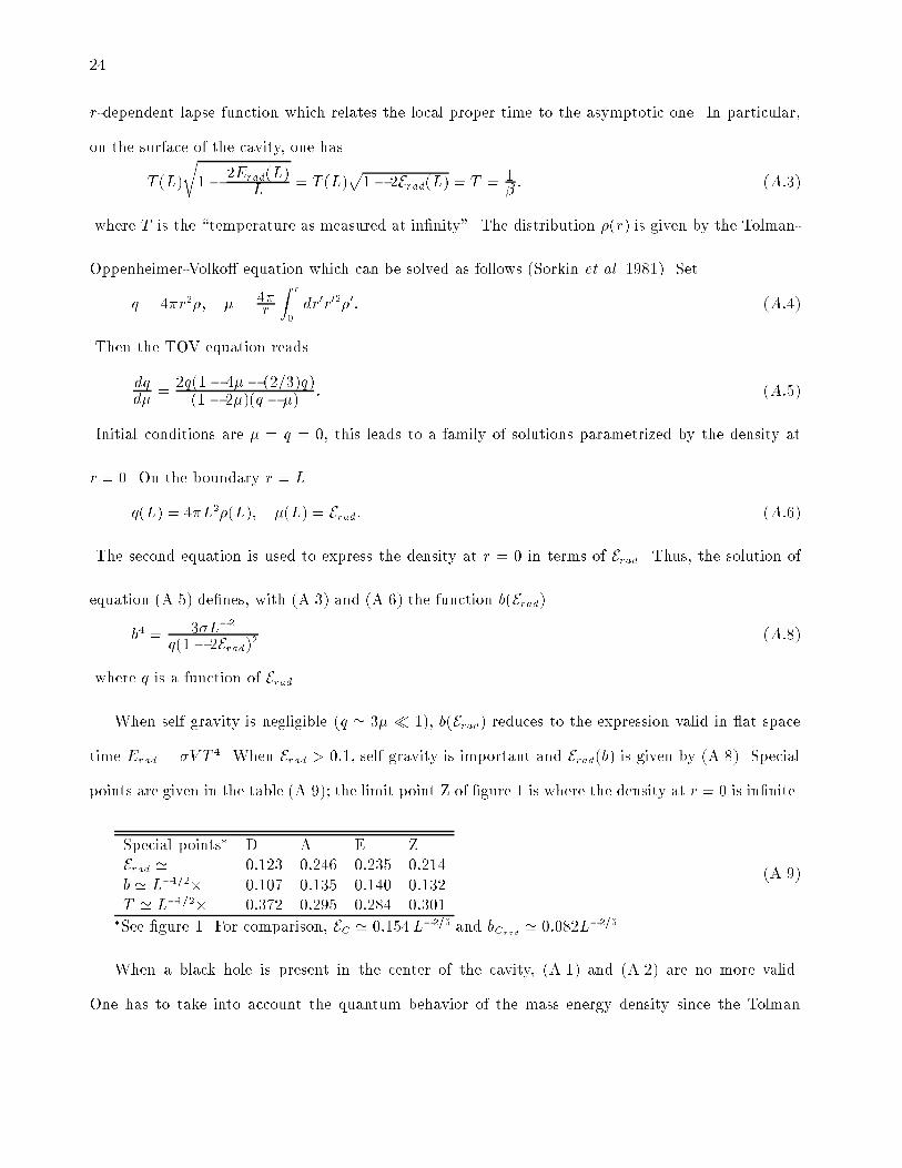
r-dependent lapse function which relates the local proper time to the asymptotic one. In particular,

on the surface of the cavity, one has

T (L)

r1� 2Erad(L)

L = T (L)p1� 2Erad(L) = T = 1

�: (A:3)

where T is the \temperature as measured at in�nity". The distribution �(r) is given by the Tolman-

Oppenheimer-Volko� equation which can be solved as follows (Sorkin et al. 1981). Set

q = 4�r2�; � = 4�r

Z r

0dr0r02�0: (A:4)

Then the TOV equation reads

dqd�

=2q(1� 4�� (2=3)q)(1� 2�)(q � �)

: (A:5)

Initial conditions are � = q = 0, this leads to a family of solutions parametrized by the density at

r = 0. On the boundary r = L

q(L) = 4�L2�(L); �(L) = Erad: (A:6)

The second equation is used to express the density at r = 0 in terms of Erad. Thus, the solution of

equation (A.5) de�nes, with (A.3) and (A.6) the function b(Erad)

b4 = 3�L�2

q(1� 2Erad)2 (A:8)

where q is a function of Erad.

When self gravity is negligible (q ' 3� � 1), b(Erad) reduces to the expression valid in at space

time Erad = �V T 4. When Erad > 0:1, self gravity is important and Erad(b) is given by (A.8). Special

points are given in the table (A.9); the limit point Z of �gure 1 is where the density at r = 0 is in�nite.

Special points� D A E ZErad ' 0:123 0:246 0:235 0:214b ' L�1=2� 0:107 0:135 0:140 0:132T ' L�1=2� 0:372 0:295 0:284 0:301

(A.9)

�See �gure 1. For comparison, EC ' 0:154L�2=5 and bCrad ' 0:082L�2=5.

When a black hole is present in the center of the cavity, (A.1) and (A.2) are no more valid.

One has to take into account the quantum behavior of the mass energy density since the Tolman

25

relations certainly break down near the horizon. The quantum version of the density is provided by

the expectation value of the time-time component of the stress energy tensor in the so-called Hartle-

Hawking \vacuum" (Howard 1984). One �nds �rst that the contribution to the gravitational mass for

2Mbh < r < 6Mbh is of the order of M�1bh (in our units, it means b�1) and secondly that for r > 6Mbh

one may approximate the mass energy density by (A.2). Thus one may approximate (5) by

m(r;Mbh) =Mbh +R r6Mbh

dr0r02M4bh(1� 2Mbh=r

0)�2: (A:10)

(again for cavities with L > 106). We have also neglected in (A.10) the self-gravity of the radiation.

For b > bC, this is certainly valid since Erad < E=5 and since EC � L=2. For smaller black holes

(Ebh < (4=5)E), the con�gurations are unstable and it is therefore useless to calculate the corrections.

From (A.10) and for b > bC , it is easy to verify that the corrections to b(E) are small and have no

e�ect on thermodynamic stability limits. The reader might consult Page (1992) to �nd an explicit

evaluation of corrections to the entropy.

We now give the derivation of (CV )A appearing in equation (52). We use equation (A.8) with

equation (A.6) and obtain the following expression for dE=db (we now drop the index rad)

3�L�2

4b3dEdb

=q(1� 2E)3(q � E)2(8

3q � 1 + 2E)

: (A:11)

Using again (A.6) with (49), we also obtain for dq=db

3�L�2

4b3dqdb

=q2(1� 2E)2(1� 4E � 2

3q)

(8

3q � 1 + 2E)

: (A:12)

These two equations give us a means to calculate the second derivative of d2E=db2�3�L�2

4b3d2qdb2

�= @@q

264q(1� 2E)3(q � E)

2(8

3q � 1 + 2E)

375�dqdb

�A

: (A:13)

At point A, the �rst derivative is zero

(�CV )A = 64�L2bAEA(1� 2EA)1� 14

3EA

�u: (A:14)

With bA given in the above table, one has thus

(�CV )A ' 23L3=2(��u): (A:15)

26

27

References

Balbinot R and Barletta A 1989 Class.Quantum Grav.195 203

Brown J D, Comer G L, Melmed J, Martinez E A, Whiting B F and York J W 1990 Class.Quantum

Grav. 7 1433

Callen H B 1985 Thermodynamics and introduction to thermostatics, p.425 (Wiley: New York)

Carlip S and Teitelboim G 1993 The O�-shell Black Hole gr-qc 9312002

Chandrasekhar S 1972 in General Relativy ed L O'Raifeartaigh (Clarendon Press)

Cocke W J 1965 Ann Inst Henri Poincar�e 283

Davies P C W 1977 Proc.Roy. Soc.Lond. A353 499

Gibbons G W and Hawking S W 1977 Phys. Rev.D 15 2752

Gibbons G W and Perry M J 1978 Proc. Roy. Soc. Lond. A 358 467

Hawking S W 1976 Phys. Rev.D 13 191

Hawking S W 1978 Phys. Rev.D 18 1747

Horwitz G and Katz J 1978 Astrophys. J. 222 941

Horwitz G and Weil D 1982 Phys. Rev. Let. 48 219

Howard K W 1984 Phys. Rev.D 30 2532

Kaburaki O, Okamoto I and Katz J 1993 Phys. Rev.D 47 2234

Katz J 1978 Mon.Not.R.Astron. Soc. 183 765

|||1979 Mon.Not. R.Astron.Soc. 189 817

Katz J and Manor Y 1975 Phys. Rev.D 12 956

Katz J, Okamoto I and Kaburaki O 1993 Class.Quantum Grav. 10 1323

Klein O 1947 Ark.Mat. Astr. Fys.A 34 1

Landau L D and Lifshitz E M 1980 Statistical physics 3rd ed (Pergamon: Oxford)

Landsberg P T 1990 Thermodynamics and statistical mechanics (Dover)

Ledoux P 1958 Stellar stability in Handbuch der Physik ed Flugge S 51

Lynden-Bell D and Wood R 1968 Mon.Not.R.Astron. Soc. 138 495

28

Lyttleton R A 1953 Theory of rotating uid masses (Cambridgr University Press)

Okamoto I and Kaburaki O 1990 Mon.Not. R.Astron. Soc. 247 244

Okamoto I, Katz J and Parentani R 1994 \A Comment on Fluctuations and Stability with Application

to Superheated Black Holes" Preprint

Page D N 1992 in Black hole physics eds De Sabatta V and Zhang Z (Kluwer Holland)

Parentani R 1994 \The Inequivalence of Thermodynamic Ensembles" Preprint

Piran T and Wald R M 1982 Phys Let A 90 20

Regge T and Teitelboim G 1974 Ann. Phys. 88 286

Schumacher B, Miller W A and Zurek W H 1992 Phys.Rev.D 46 1416.

Sorkin R D, Wald R M and Zhang Z J 1982 Gen Rel Grav 13 1127

Thompson J M T 1979 Phil Trans R Soc Lond 292 1386.

Tolman C 1934 Relativity, thermodynamics and cosmology p.318 (Clarendon)

York J W 1985 Phys. Rev.D 31 775

York J W 1986 Phys. Rev.D 33 2092

Zurek W H 1980 Phys Let A 77 399

29

Figure captions

Figure 1. b(Ebh), b(Erad) and b(E) are drawn for L = 106, in �gure 1a for E <� 10�3 and in �gure 1b

for E >� 10�1. Between E = 10�3 and 10�1, b(Erad) and b(E) come closer and closer to the point that in

�gure 1b the two lines are indistinguishable. The line b(E) through points FCQDAZ is a counterclock

inward spiral. The dotted line in the lower left hand corner of �gure 1b is the non-relativistic (no

selfgravity) b(Erad) for comparison.

Figure 2. b(Ebh;J ), b(Erad;J ) and b(E ;J ) curves for constant angular momentum J and L =

2:65 � 104. The low value of L is to make clear �gures. Figure 2a is for J = 1=40 and �gure 2b is

for J = 1=8. Both lines are drawn with the same limits of b and E , showing the displacement to

right for increasing J of the linear series b(Erad;J ), b(E ;J ) and of the point C. Once the equilibrium

con�gurations leave the linear series b(Ebh;J ), the black hole starts to loose mass with respect to the

radiation, see �gure 3.

Figure 3. This �gure displays two lines: (a) The minimum of energy EC(J ) as a function of increasing

angular momentum. The scale of EC displayed on the left is the same as in �gure 2. The curve is

parametrized in real values of EC . Notice that beyond J = 3=16 � 0:2, the energy EC is highly

relativistic and the non-relativistic curve is likely to be di�erent. (b) The ratio EbhC=EC = bC=ECwith its scale displayed on the right. For J = 0, EbhC=EC = 4=5; this is well above the limits of the

drawing.