LawrenceLivermoreNationalLaboratory

U.S. Department of Energy

Approved for public release; further dissemination unlimited

UCRL-ID-153656

Thermal Scattering Law Data: Implementation and Testing using the Monte Carlo neutron transport

codes COG, MCNP and TART

D. E. Cullen L. F. Hansen

E. M. Lent E. F. Plechaty

May 17, 2003

DISCLAIMER This document was prepared as an account of work sponsored by an agency of the United States Government. Neither the United States Government nor the University of California nor any of their employees, makes any warranty, express or implied, or assumes any legal liability or responsibility for the accuracy, completeness, or usefulness of any information, apparatus, product, or process disclosed, or represents that its use would not infringe privately owned rights. Reference herein to any specific commercial product, process, or service by trade name, trademark, manufacturer, or otherwise, does not necessarily constitute or imply its endorsement, recommendation, or favoring by the United States Government or the University of California. The views and opinions of authors expressed herein do not necessarily state or reflect those of the United States Government or the University of California, and shall not be used for advertising or product endorsement purposes. This work was performed under the auspices of the U. S. Department of Energy by the University of California, Lawrence Livermore National Laboratory under Contract No. W-7405-Eng-48.

This report has been reproduced directly from the best available copy.

Available to DOE and DOE contractors from the Office of Scientific and Technical Information

P.O. Box 62, Oak Ridge, TN 37831 Prices available from (423) 576-8401

http://apollo.osti.gov/bridge/

Available to the public from the National Technical Information Service

U.S. Department of Commerce 5285 Port Royal Rd.,

Springfield, VA 22161 http://www.ntis.gov/

OR

Lawrence Livermore National Laboratory

Technical Information Department’s Digital Library http://www.llnl.gov/tid/Library.html

UCRL-ID-153656

Thermal Scattering Law Data:

Implementation and Testing using the Monte Carlo neutron transport

codes COG, MCNP and TART

by Dermott E. Cullen Luisa F. Hansen Edward M. Lent

Ernest F. Plechaty

University of California Lawrence Livermore National Laboratory

P.O. Box 808 Livermore, CA 94550

Contact:

E.Mail: cullen1@llnl.gov Website: http://www.llnl.gov/cullen1

May 17, 2003

Abstract

Recently we implemented the ENDF/B-VI thermal scattering law data in our neutron transport codes COG and TART. Our objective was to convert the existing ENDF/B data into double differential form in the Livermore ENDL format. This will allow us to use the ENDF/B data in any neutron transport code, be it a Monte Carlo, or deterministic code. This was approached as a multi-step project. The first step was to develop methods to directly use the thermal scattering law data in our Monte Carlo codes. The next step was to convert the data to double-differential form. The last step was to verify that the results obtained using the data directly are essentially the same as the results obtained using the double differential data. Part of the planned verification was intended to insure that the data as finally implemented in the COG and TART codes, gave the same answer as the well known MCNP code, which includes thermal scattering law data. Limitations in the treatment of thermal scattering law data in MCNP have been uncovered that prevented us from performing this part of our verification.

1

Introduction Recently we implemented the ENDF/B-VI [1] thermal scattering law data in our neutron transport codes COG [2] and TART [3]. Our objective was to convert the existing ENDF/B data into double differential form in the Livermore ENDL format [4]. This will allow us to use the ENDF/B data in any neutron transport code, be it a Monte Carlo, or deterministic code. This was approached as a multi-step project. The first step was to develop methods to directly use the thermal scattering law data in our Monte Carlo codes. The next step was to convert the data to double-differential form. The last step was to verify that the results obtained using the data directly are essentially the same as the results obtained using the double differential data. Part of the planned verification was intended to insure that the data as finally implemented in the COG and TART codes, gave the same answer as the well known MCNP [5] code, which includes thermal scattering law data. Limitations in the treatment of thermal scattering law data in MCNP have been uncovered that prevented us from performing this part of our verification.

The importance of bound and Free Atom Models

Both bound and free atom models are important for use in neutron transport calculations. When thermal scattering law data is available to describe bound atoms, it should be used in the calculations. Because thermal scattering law data is only available for a few ENDF/B [6] materials, we must rely on using a free atom model to describe thermal effects in all other cases. Currently there are 328 materials in ENDF/B [7] for which we have evaluated neutron data, while thermal scattering law data exist for only six of these materials. These simple statistics show how heavily we must rely on free atom scattering. It should be mentioned that there is more thermal scattering law data available, but none of it is specifically for use with any of the 328 materials in ENDF/B-VI. For example, data is available for para and ortho hydrogen, and methane, which are not of interest to us for use in our applications. The six materials covered in this report are based upon their common use in our thermal neutron system applications.

Do Not Misuse Thermal Scattering Law Data Care should be used when using the available thermal scattering law data. These data are intended ONLY to be used when describing the binding of atoms in specific materials. Binding effects can vary appreciable for the same atom bound to different materials, as we will see below for the case of hydrogen (H) bound in polyethylene (CH2) or water (H2O), as well as for beryllium (Be) bound in Be metal or BeO. Specifically, do not assume that the binding of hydrogen (H) in any other material can be better described by

2

using the bound CH2 or H2O data, rather than by free atom scattering, particularly if a Debye effective temperature is used. Again, CAVEAT EMPTOR.

Identification of Materials in ENDL

Materials in ENDL are identified using the same convention as that used by ENDF/B. Each material is identified by a combination of its atomic number, Z, and its atomic weight, A, in the form 1000*Z + A. For example, hydrogen (Z=1, A=1) is identified as ZA = 1001. Similarly deuterium (Z=1, A=2) is identified as ZA = 1002. The six materials with thermal scattering law data that have been added to ENDL have been somewhat arbitrarily assigned special ZA numbers. The convention that we used is that they have the same ZA as the free atom data + 900 for the first special material that we encounter, + 800 for the second special material. For example, for hydrogen the first material we encountered was H in CH2, which has been assigned ZA = 1901; the second material encountered for hydrogen was H in H2O, which has been assigned ZA = 1801; the first material encountered for carbon was C in graphite, which has been assigned 6912. In ENDL each of these materials is a complete evaluation (not just low energy thermal scattering law data). For everything except elastic scattering each bound material is identical to the free atom data, e.g., capture is the same at all energies. Above some cutoff energy (in the eV range) the elastic scattering for each material is identical to the free atom data. Below the cutoff energy the elastic cross section is set to zero, and replace by the inelastic thermal scattering law data. Using this convention these six materials are identified in ENDL, in ascending assigned ZA order, Cutoff Material Bound Free Energy (eV) H in H2O 1801 1001 4.0 H in CH2 1901 1001 1.5 D in D2O 1902 1002 1.5 Be in Be metal 4809 4009 2.0 Be in BeO 4909 4009 2.0 C in graphite 6912 6012 2.0 O in BeO 8916 8016 2.0 To perform calculations using bound rather than free data, with this convention users need merely replace the free ZA by the bound ZA in the definition of materials. For most of the ENDF/B-VI thermal scattering law data this involves replacing only one ZA by another, e.g., H in CH2. The exception is BeO, where the thermal scattering law data represents the combined effect of both Be and O; in this case both Be and O MUST be

3

replaced. For example, free H2O is 2 atoms 1001 to 1 atom 8016, whereas H bound in H2O is 2 atoms 1801 to 1 atom 8016. The one exception is that for BeO users MUST replace both Be and O; free BeO is 1 atom 4009 to 1 atom 8016, whereas Be and O bound in BeO is 1 atom 4909 to 1 atom 8916. In the case of BeO the thermal scattering law includes the effect of both Be and O; for use in ENDL the thermal scattering law is included in 4909, and 8916 has zero scattering below the cutoff; see the cross sections below.

Thermal scattering law definitions The following is a brief list of thermal scattering law definitions. For our purposes we need not define in detail all of the terms in these equations; we are only interested in showing the function form of each type of data. For complete details of all definitions see the ENDF/B formats and procedures manual, ENDF-102 [6]. Coherent Elastic Scattering

ΩdEdd σ2 ),,'( TEE µ>− = ∑

<

=

−−EEj

jEEjTsj

E 12/)'()()(1 πδµµδ (1)

where,

jµ = 1 - EEj2 (2)

In coherent elastic scattering there is no change in neutron energy (E’ = E), and the neutrons can only scatter through a series of discrete angles µ( = )jµ , giving rise to “strange” looking angular distributions. Discrete changes, “jumps”, in the cross section at a series of Bragg edges, E = Ej are observed. This representation is used for the crystalline materials, Be in Be metal and BeO, and C in graphite, and can be recognized in the cross sections shown below by the discrete “jumps” in the cross section (see Figs. 4, 5 and 7). Incoherent Elastic Scattering

ΩdEdd σ2 ),,'( TEE µ>− = σ b πδµ 4/)]'()1)(('2[ EETEWExp −−− (3)

where σ b is the bound atom cross section. The integrated cross section is

)(Eσ =σ b '4

)'4(EW

EWExp −−1 , note that as E 0, )(Eσ σ b (4)

4

Here there is no change in neutron energy (E’ = E), and the neutrons scatter through continuous angles, with an angular distribution that varies from σ b π4/ at 1=µ , to

σ b π4/]'4[ EWExp − at µ = -1, as E 0, the angular distribution becomes isotropic,

σ b π4/ . This representation is used for H in CH2, and can be recognized in the cross sections shown in Fig. 2, below, by the cross section becoming constant at low energy, σ b π4/ . H in H2O and D in D2O do not include coherent or incoherent elastic scattering.

Incoherent Inelastic Scattering

ΩdEdd σ2 ),,'( TEE µ>− = M∑

=

NS

n 0n σ bn TTSnExpEE πβαβ 4/),,()2/(/' − (5)

Here both energy and direction can vary continuously. This representation is used in all six materials, and is what we will refer to below as ),( βαS . In summary, these are the only three models used with the ENDF/B thermal scattering law data. Two of these are elastic, allowing change in neutron direction, but not allowing any change in energy. The only model allowing change in direction and energy is what we will refer to as ),( βαS . Our experience has been that it is fairly easy to represent all of this data in the ENDL format as inelastic double-differential data, for use in our applications.

Comparison of Bound and Free Cross Sections

First let’s look at the difference in cross sections for free atom and bound atom cross sections. Here we limit ourselves to only discussing the difference between free and bound data in our data files; we will not discuss the detailed theory of free atom or bound neutron scattering. At low energy the “cold” (0 Kelvin) free atom scattering cross sections are generally constant; for light isotopes this constant cross section can extend to quite high energy, e.g., to the keV range. Due to Doppler broadening the low energy free atom cross sections increase with temperature, and well below the thermal energy will vary inversely with speed (|velocity|), i.e., 1/v. The basic shape of the free atom cross section is the same for all materials, and the low energy increase due to Doppler broadening can be characterized by a single dimensionless parameter, AE/KT, where A is atomic weight, E is energy, and KT is temperature in energy units [8].

5

In contrast the bound cross section varies from one material to another, even for the same isotope bound in different materials, as we will see for hydrogen bound in water (H2O) versus hydrogen bound in polyethylene (CH2). As described above, the model used for ENDF/B thermal scattering law data is quite simple,

1) The cross sections for bound and free scattering are identical above a given cutoff energy of a few eV, equal to the elastic scattering cross section that is used at higher energies. Below the cutoff energy this cross section abruptly drops to zero.

2) Below the cutoff energy the cross section is represented by one or two processes,

one process produces an energy spectrum of scattered neutrons (as occurs with free atom scatter), the other process can cause neutrons to change direction with no energy loss (as if the neutrons scatter off of an infinitely heavy target). As we will see below, all the materials for which we have thermal scattering law data include the one process that produces an energy spectrum, but only for some of these materials the second process is included.

If you are used to neutrons slowing down you will be familiar with the terminology elastic and inelastic scattering. During slowing down a collision is elastic if there is no energy change in the center-of-mass frame of reference; it is inelastic if there is a change of energy; generally a loss of energy, leaving the nucleus in an excited state. In the laboratory frame of reference both elastic and inelastic scattering result in a loss of energy by the neutron. Unfortunately, exactly the same terminology is used when describing bound cross sections at low energy, but here it has a different meaning. For bound scattering at low energy, “Elastic” scattering results in no energy change in the laboratory frame of reference, and “Inelastic” results in a change of energy, which can be positive (the neutron energy increases) or negative (the neutron energy decreases). In summary: elastic scattering at higher energy results in a change of direction and a loss of energy while elastic scattering for bound data results in a change in direction, but no change in energy. Inelastic scattering at higher energy results in a change of direction and a loss of energy while inelastic scattering for bound data results in a change in direction and energy, where the energy change can be positive or negative. To avoid confusion, in the discussion to follow, we will NOT use the bound cross section terminology. We will try to use the terminology used to describe neutrons slowing down at higher energies. In particular, when we refer to the “elastic” cross section, we mean the cross section that is identical for both free and bound scattering above some cut-off energy in the eV range. Below this energy we will refer to the bound cross sections as “inelastic”, in the sense that they do not correspond to elastic free atom scattering.

6

Comparison of Bound and Free H in H2O Cross Sections

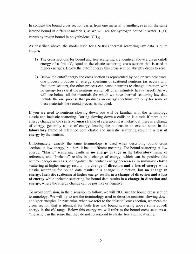
Figure 1 compares the hydrogen (H) cross section for free H and H bound in H2O (water). In this case the bound and free elastic cross sections are identical above 4 eV. Below this point only one process is used to define the bound cross section where a scattered neutron can change both direction and energy. At 4 eV the bound cross section abruptly switches to an inelastic form where S( βα , ) (eq. 5) is used to describe the secondary distribution of neutrons in direction and energy. Physically the “bump” in the bound cross section in the 1 to 0.001 eV range is usually described as due to the effective atomic weight (A) increasing from 1 near and above an eV, to a larger number by 0.001 eV. The definition of the elastic cross section included a term that depends on the atomic weight (A) and is proportional to [A/(A+1)]2. For A = 1, this is 1/4, resulting in the 20 barns cross section above about 1 eV; in contrast for a large A this is about 1, resulting in the 80 barn cross section near 0.001 eV. For water all of this variation is included in the definition of S( βα , ) (eq. 5). Water is not a crystalline material, so fairly smooth variation of the cross sections is expected, as observed in Fig. 1; later we will contrast this behavior with the bound cross section for Be and graphite, both crystalline materials. In addition to the binding effect, Doppler broadening also contributes; at very low energies the Doppler broadened free elastic and bound inelastic cross section are very similar in shape and magnitude

Fig. 1: Comparison of Bound and Free H in H2O Cross Sections

7

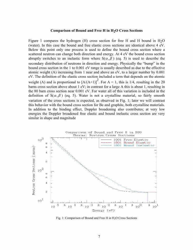
Comparison of Bound and Free H in CH2 Cross Sections Figure 2 compares the hydrogen (H) cross section for free H and H bound in CH2 (polyethylene). In this case the bound and free elastic cross sections are identical above 1.5 eV. Below this point two processes are used to define the bound cross section: 1) a scattered neutron can change both direction and energy, and 2) a neutron can only change direction with no energy loss. At 1.5 eV the bound cross section abruptly switches to an inelastic form where S( βα , ) (eq. 5) is used to describe the secondary distribution of neutrons in direction and energy. The second process with no energy loss starts at 1.5 eV as quite small and increases to about 80 barns by 0.001 eV, and then remains constant at lower energies (eq. 3). A comparison of the cross sections for H bound in H2O (Fig. 1) to the cross section for H bound in CH2 (Fig. 2) seems to be quite different as a function of energy. However, the sum of the two inelastic cross sections for CH2 is very similar to the cross section for H2O. Polyethylene, as water, is not a crystalline material, so a fairly smooth variation of the cross sections is expected and observed. In addition to the binding effect, Doppler broadening also contributes; at very low energies the Doppler broadened free elastic and bound inelastic cross section are very similar in shape but much smaller in magnitude

Fig. 2: Comparison of Bound and Free H in CH2 Cross Sections

8

Comparison of Bound and Free D in D2O Cross Sections

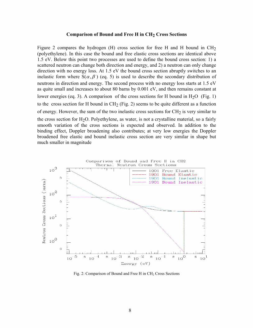
. Figure 3 compares the deuterium (D) cross section for free D and D bound in D2O (heavy water). The model for D bound in D2O is very similar to the model for H bound in H2O described above. In this case the bound and free elastic cross sections are identical above 1.5 eV. Below this point only one process is used to define the bound cross section where a scattered neutron can change both direction and energy. At 1.5 eV the bound cross section abruptly switches to an inelastic form where S( βα , ) is used to describe the secondary distribution of neutrons in direction and energy. The “bump” in the bound cross section in the 1 to 0.001 eV range is usually described as due to the effective atomic weight (A) increasing from 2 near and above an eV, to a large number by 0.001 eV. The definition of the elastic cross section included a term that depends on the atomic weight (A) and is proportional to [A/(A+1)]2. For A = 2, this is 4/9, resulting in the 3.4 barns cross section above about 1 eV; in contrast for a large A this is about 1, resulting in the 7.6 barns cross section near 0.001 eV. Since heavy water is not a crystalline material, a fairly smooth variation of the cross sections is observed. Doppler broadening also contributes to the cross section; at very low energies the Doppler broadened free elastic and bound inelastic cross sections are very similar in shape, but much lower in magnitude.

Fig. 3: Comparison of Bound and Free D in D2O Cross Sections

9

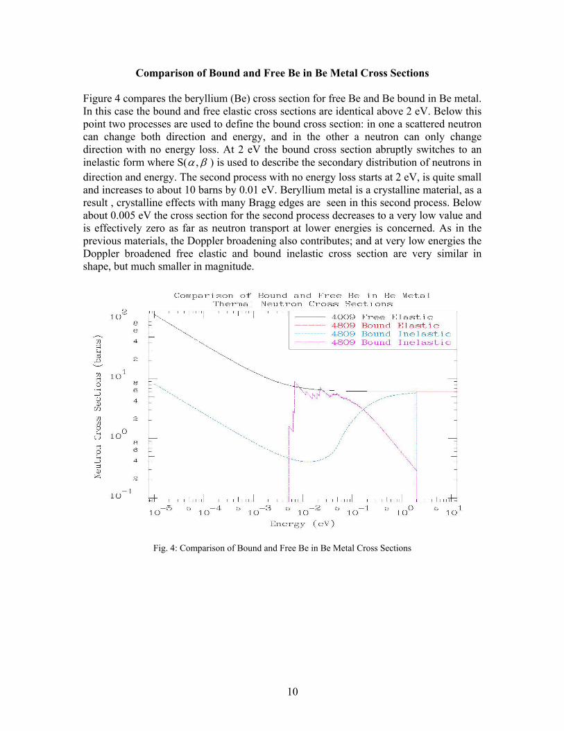
Comparison of Bound and Free Be in Be Metal Cross Sections

Figure 4 compares the beryllium (Be) cross section for free Be and Be bound in Be metal. In this case the bound and free elastic cross sections are identical above 2 eV. Below this point two processes are used to define the bound cross section: in one a scattered neutron can change both direction and energy, and in the other a neutron can only change direction with no energy loss. At 2 eV the bound cross section abruptly switches to an inelastic form where S( βα , ) is used to describe the secondary distribution of neutrons in direction and energy. The second process with no energy loss starts at 2 eV, is quite small and increases to about 10 barns by 0.01 eV. Beryllium metal is a crystalline material, as a result , crystalline effects with many Bragg edges are seen in this second process. Below about 0.005 eV the cross section for the second process decreases to a very low value and is effectively zero as far as neutron transport at lower energies is concerned. As in the previous materials, the Doppler broadening also contributes; and at very low energies the Doppler broadened free elastic and bound inelastic cross section are very similar in shape, but much smaller in magnitude.

Fig. 4: Comparison of Bound and Free Be in Be Metal Cross Sections

10

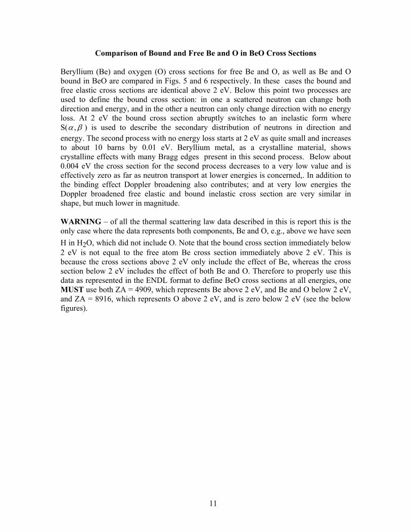
Comparison of Bound and Free Be and O in BeO Cross Sections

Beryllium (Be) and oxygen (O) cross sections for free Be and O, as well as Be and O bound in BeO are compared in Figs. 5 and 6 respectively. In these cases the bound and free elastic cross sections are identical above 2 eV. Below this point two processes are used to define the bound cross section: in one a scattered neutron can change both direction and energy, and in the other a neutron can only change direction with no energy loss. At 2 eV the bound cross section abruptly switches to an inelastic form where S( βα , ) is used to describe the secondary distribution of neutrons in direction and energy. The second process with no energy loss starts at 2 eV as quite small and increases to about 10 barns by 0.01 eV. Beryllium metal, as a crystalline material, shows crystalline effects with many Bragg edges present in this second process. Below about 0.004 eV the cross section for the second process decreases to a very low value and is effectively zero as far as neutron transport at lower energies is concerned,. In addition to the binding effect Doppler broadening also contributes; and at very low energies the Doppler broadened free elastic and bound inelastic cross section are very similar in shape, but much lower in magnitude. WARNING – of all the thermal scattering law data described in this is report this is the only case where the data represents both components, Be and O, e.g., above we have seen H in H2O, which did not include O. Note that the bound cross section immediately below 2 eV is not equal to the free atom Be cross section immediately above 2 eV. This is because the cross sections above 2 eV only include the effect of Be, whereas the cross section below 2 eV includes the effect of both Be and O. Therefore to properly use this data as represented in the ENDL format to define BeO cross sections at all energies, one MUST use both ZA = 4909, which represents Be above 2 eV, and Be and O below 2 eV, and ZA = 8916, which represents O above 2 eV, and is zero below 2 eV (see the below figures).

11

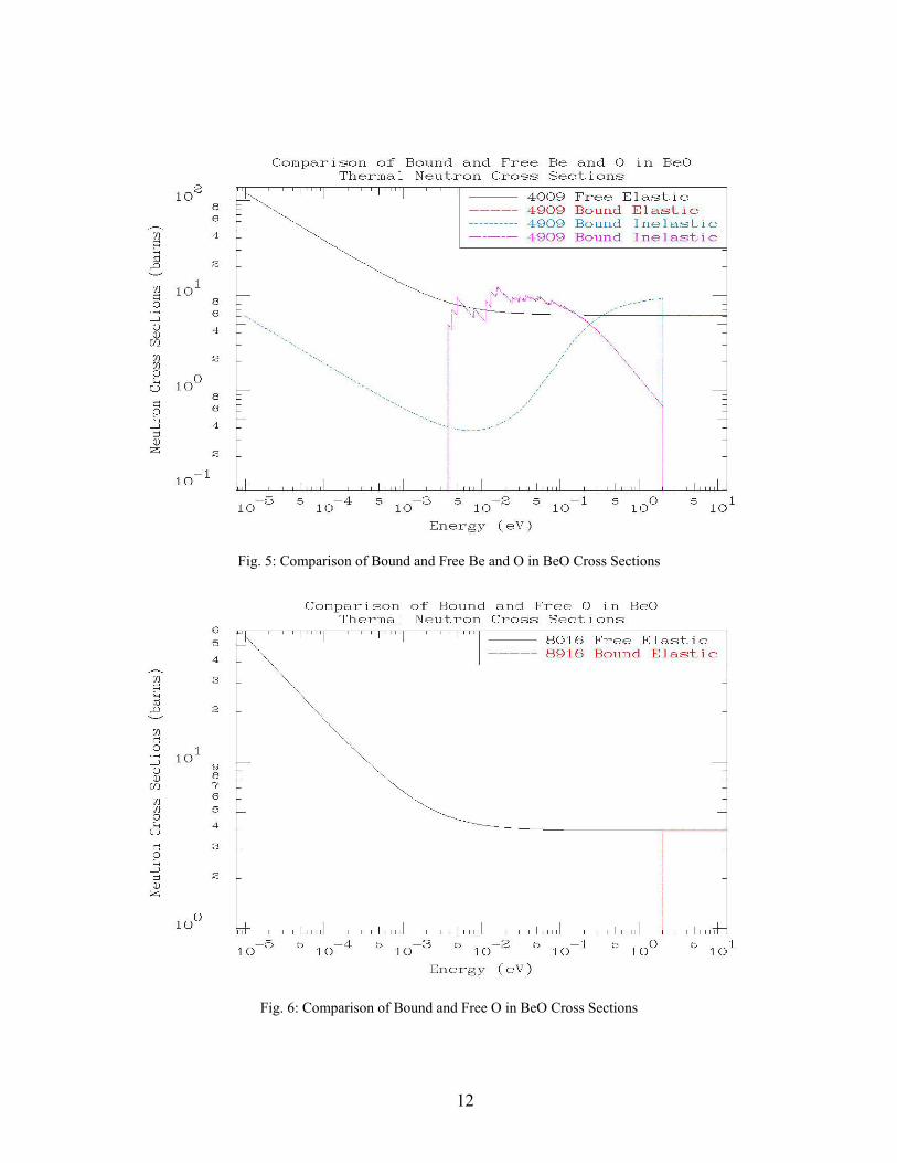
Fig. 5: Comparison of Bound and Free Be and O in BeO Cross Sections

Fig. 6: Comparison of Bound and Free O in BeO Cross Sections

12

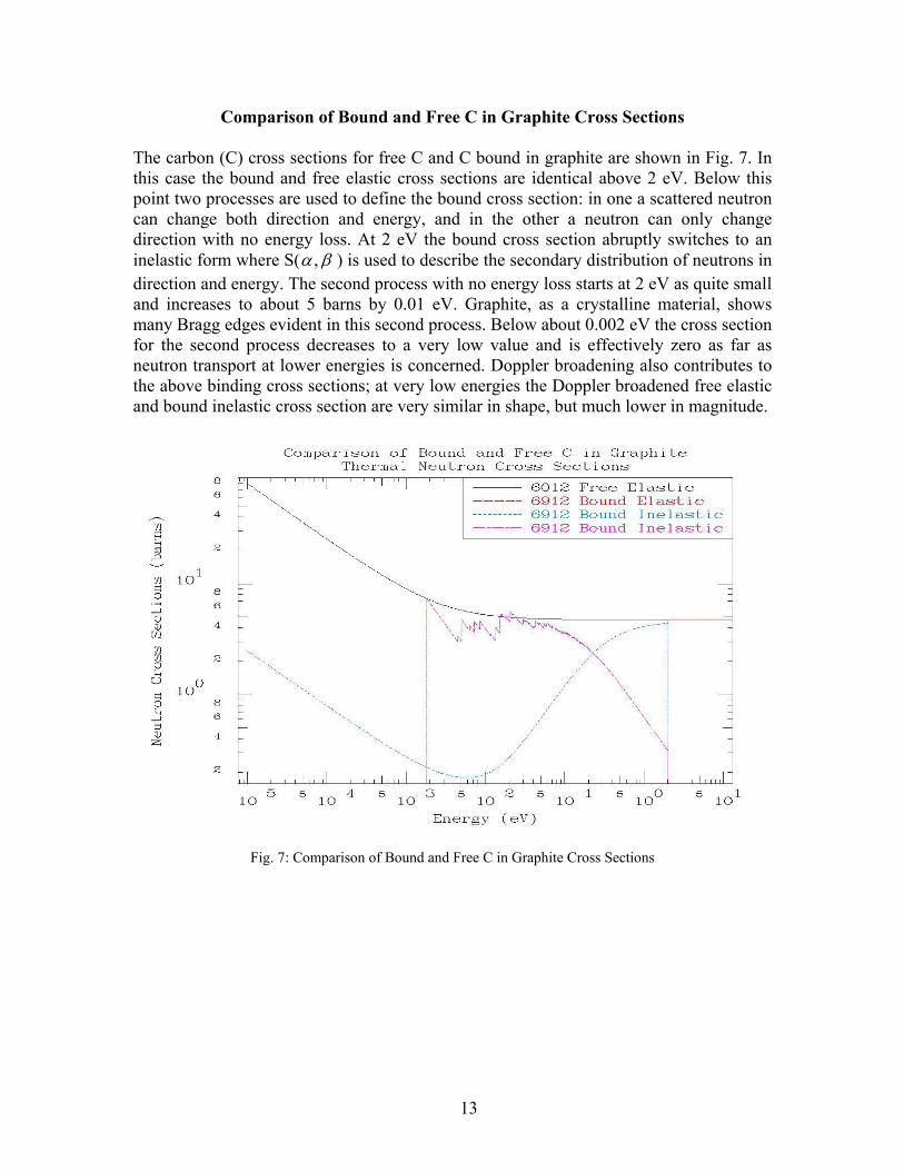
Comparison of Bound and Free C in Graphite Cross Sections The carbon (C) cross sections for free C and C bound in graphite are shown in Fig. 7. In this case the bound and free elastic cross sections are identical above 2 eV. Below this point two processes are used to define the bound cross section: in one a scattered neutron can change both direction and energy, and in the other a neutron can only change direction with no energy loss. At 2 eV the bound cross section abruptly switches to an inelastic form where S( βα , ) is used to describe the secondary distribution of neutrons in direction and energy. The second process with no energy loss starts at 2 eV as quite small and increases to about 5 barns by 0.01 eV. Graphite, as a crystalline material, shows many Bragg edges evident in this second process. Below about 0.002 eV the cross section for the second process decreases to a very low value and is effectively zero as far as neutron transport at lower energies is concerned. Doppler broadening also contributes to the above binding cross sections; at very low energies the Doppler broadened free elastic and bound inelastic cross section are very similar in shape, but much lower in magnitude.

Fig. 7: Comparison of Bound and Free C in Graphite Cross Sections

13

Test Problems

We will use two simple test problems to verify the accuracy of our results, 1) Differential results, so that we can see the single collision energy and angle results. 2) Integral results, so that we can see the results of neutrons slowing down in each material; here we are interested in both the energy and time dependent spectra. In all cases we assume room temperature conditions, i.e., an average temperature in energy units of 0.0253 eV. In each case we will compare results for the three codes, MCNP, COG and TART, using bound and free atom cross sections, to better judge where the difference between bound and free models is important. Material definitions For both problems we will use the same definitions for the materials discussed earlier, namely, CH2: 0.91 grams/cc, 2 atoms of H (bound or free) to 1 atom of C (free) H2O: 1.00 grams/cc, 2 atoms of H (bound or free) to 1 atom of O (free) D2O: 1.11 grams/cc, 2 atoms of D (bound or free) to 1 atom of O (free) Be Metal: 1.85 grams/cc, pure Be (bound or free) BeO: 2.81 grams/cc, 1 atom of Be (bound or free) to 1 atom of O (bound or free) C: 1.67 grams/cc, pure C (bound or free) Differential Test Problem The differential results were obtained running what are called “broomstick” calculations. An extremely long, narrow cylinder of each material (i.e., a broomstick) was used and the neutrons were directed monodirectionally along the axis of the cylinder. The cylinder is defined to be so long that essentially all neutrons are forced to have a collision within the cylinder, and the cylinder is defined to be so narrow that every scatter causes the neutron to scatter out of the cylinder without undergoing any more collisions. In this case by measuring the “leakage” from the cylinder we are directly measuring the single collision distribution. Both, the energy spectrum and the angular distribution are of interest in this case. The differential test problem has the following features: 1) A cylinder 10

5 cm in length, and 10

-8 cm in radius.

2) A point source is located on the axis of the cylinder 103 cm from one end (to avoid

any possible end effects). 3) The neutron source is monoenergetic at 0.0253 eV, and monodirectional, directed along the axis of the cylinder. Neutrons “leaking” from the cylinder are tallied according to:

14

a) the energy spectrum in 50 energy bins per energy decade, equally spaced in the log of the energy, between 10

-5 eV and 20 MeV, and

b) the cosine of the angle relative to the axis of the cylinder, from –1 (backscatter) to +1 (forward scatter), in 200 equally spaced cosine bins; note that equal cosine intervals corresponds to equal solid angles.

15

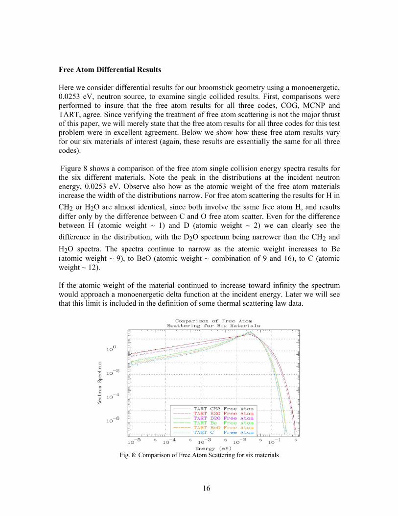
Free Atom Differential Results Here we consider differential results for our broomstick geometry using a monoenergetic, 0.0253 eV, neutron source, to examine single collided results. First, comparisons were performed to insure that the free atom results for all three codes, COG, MCNP and TART, agree. Since verifying the treatment of free atom scattering is not the major thrust of this paper, we will merely state that the free atom results for all three codes for this test problem were in excellent agreement. Below we show how these free atom results vary for our six materials of interest (again, these results are essentially the same for all three codes). Figure 8 shows a comparison of the free atom single collision energy spectra results for the six different materials. Note the peak in the distributions at the incident neutron energy, 0.0253 eV. Observe also how as the atomic weight of the free atom materials increase the width of the distributions narrow. For free atom scattering the results for H in CH2 or H2O are almost identical, since both involve the same free atom H, and results differ only by the difference between C and O free atom scatter. Even for the difference between H (atomic weight ~ 1) and D (atomic weight ~ 2) we can clearly see the difference in the distribution, with the D2O spectrum being narrower than the CH2 and H2O spectra. The spectra continue to narrow as the atomic weight increases to Be (atomic weight ~ 9), to BeO (atomic weight ~ combination of 9 and 16), to C (atomic weight ~ 12). If the atomic weight of the material continued to increase toward infinity the spectrum would approach a monoenergetic delta function at the incident energy. Later we will see that this limit is included in the definition of some thermal scattering law data.

Fig. 8: Comparison of Free Atom Scattering for six materials

16

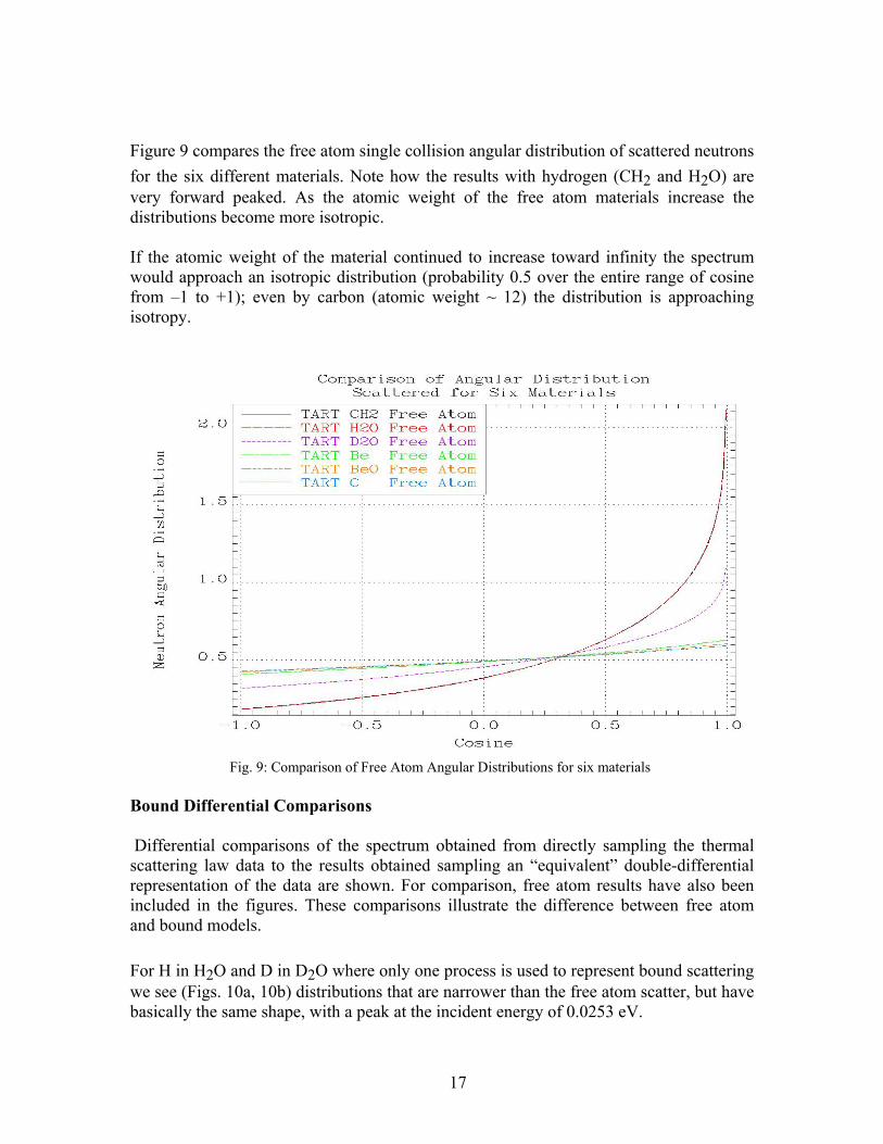
Figure 9 compares the free atom single collision angular distribution of scattered neutrons for the six different materials. Note how the results with hydrogen (CH2 and H2O) are very forward peaked. As the atomic weight of the free atom materials increase the distributions become more isotropic. If the atomic weight of the material continued to increase toward infinity the spectrum would approach an isotropic distribution (probability 0.5 over the entire range of cosine from –1 to +1); even by carbon (atomic weight ~ 12) the distribution is approaching isotropy.

Fig. 9: Comparison of Free Atom Angular Distributions for six materials Bound Differential Comparisons Differential comparisons of the spectrum obtained from directly sampling the thermal scattering law data to the results obtained sampling an “equivalent” double-differential representation of the data are shown. For comparison, free atom results have also been included in the figures. These comparisons illustrate the difference between free atom and bound models. For H in H2O and D in D2O where only one process is used to represent bound scattering we see (Figs. 10a, 10b) distributions that are narrower than the free atom scatter, but have basically the same shape, with a peak at the incident energy of 0.0253 eV.

17

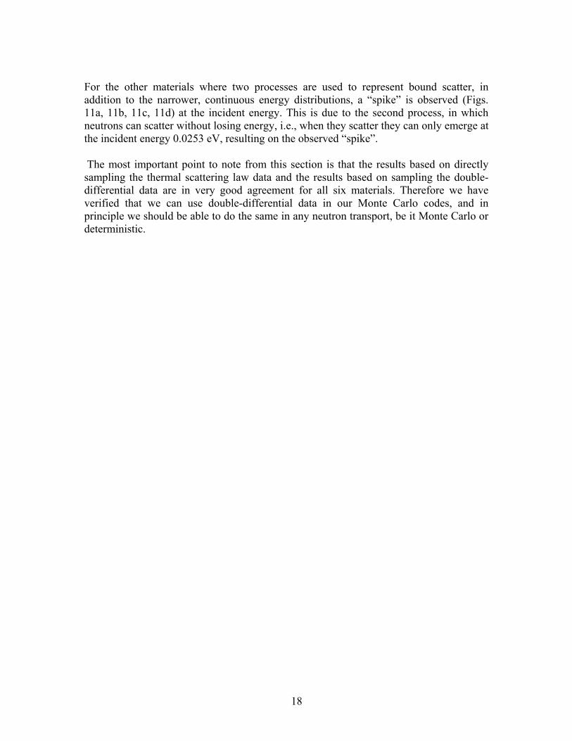
For the other materials where two processes are used to represent bound scatter, in addition to the narrower, continuous energy distributions, a “spike” is observed (Figs. 11a, 11b, 11c, 11d) at the incident energy. This is due to the second process, in which neutrons can scatter without losing energy, i.e., when they scatter they can only emerge at the incident energy 0.0253 eV, resulting on the observed “spike”. The most important point to note from this section is that the results based on directly sampling the thermal scattering law data and the results based on sampling the double-differential data are in very good agreement for all six materials. Therefore we have verified that we can use double-differential data in our Monte Carlo codes, and in principle we should be able to do the same in any neutron transport, be it Monte Carlo or deterministic.

18

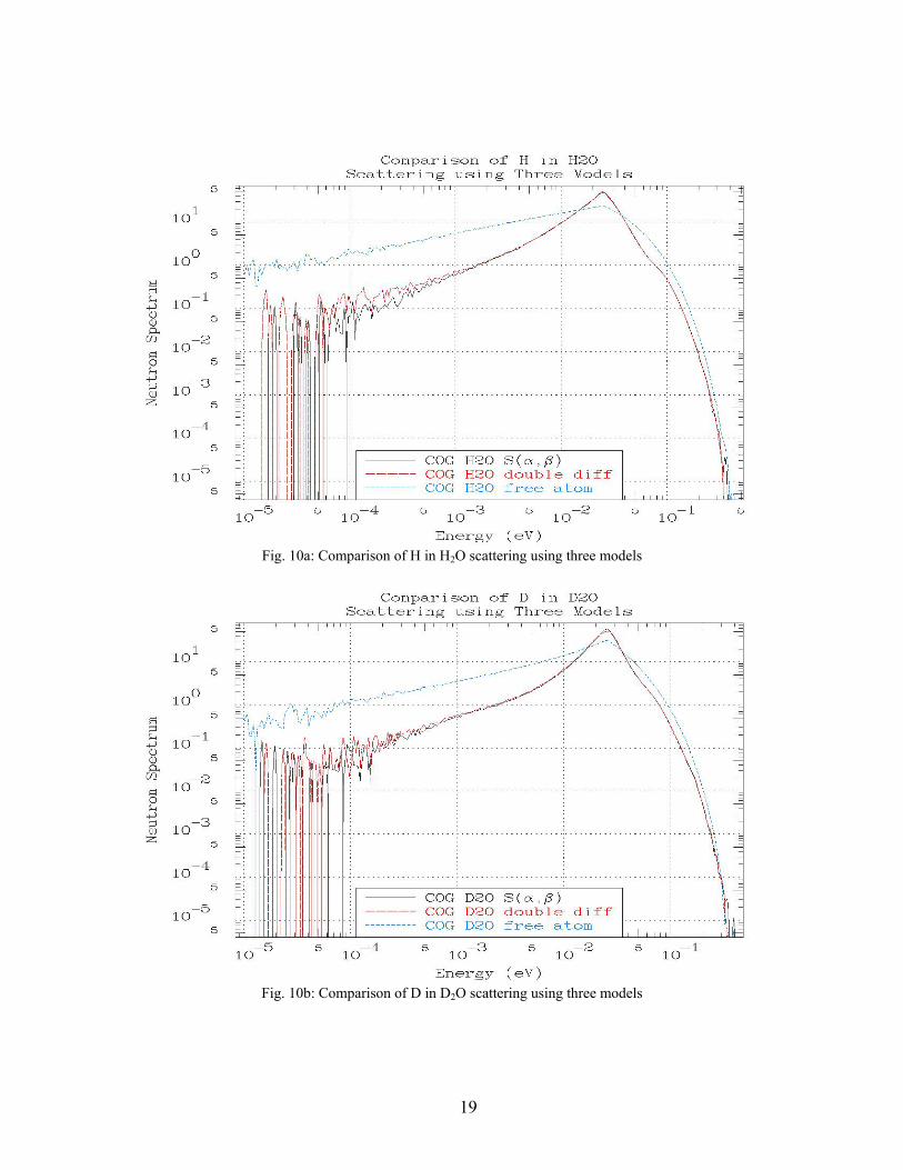
Fig. 10a: Comparison of H in H2O scattering using three models

Fig. 10b: Comparison of D in D2O scattering using three models

19

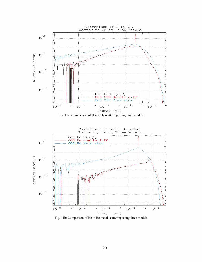
Fig. 11a: Comparison of H in CH2 scattering using three models

Fig. 11b: Comparison of Be in Be metal scattering using three models

20

Fig. 11c: Comparison of Be and O in BeO scattering using three models

Fig. 11d: Comparison of C in graphite scattering using three models

21

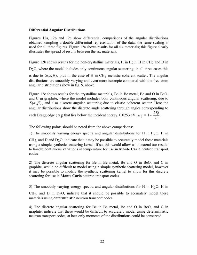
Differential Angular Distributions Figures 12a, 12b and 12c show differential comparisons of the angular distributions obtained sampling a double-differential representation of the data; the same scaling is used for all three figures. Figure 12a shows results for all six materials; this figure clearly illustrates the spread of results between the six materials. Figure 12b shows results for the non-crystalline materials, H in H2O, H in CH2 and D in

D2O, where the model includes only continuous angular scattering; in all three cases this

is due to ),( βαS , plus in the case of H in CH2 inelastic coherent scatter. The angular distributions are smoothly varying and even more isotropic compared with the free atom angular distributions show in fig. 9, above. Figure 12c shows results for the crystalline materials, Be in Be metal, Be and O in BeO, and C in graphite, where the model includes both continuous angular scattering, due to

),( βαS , and also discrete angular scattering due to elastic coherent scatter. Here the angular distributions show the discrete angle scattering through angles corresponding to

each Bragg edge (µ j) that lies below the incident energy, 0.0253 eV; µ j = 1 - EEj2 .

The following points should be noted from the above comparisons: 1) The smoothly varying energy spectra and angular distributions for H in H2O, H in

CH2, and D and D2O, indicate that it may be possible to accurately model these materials using a simple synthetic scattering kernel; if so, this would allow us to extend our results to handle continuous variations in temperature for use in Monte Carlo neutron transport codes 2) The discrete angular scattering for Be in Be metal, Be and O in BeO, and C in graphite, would be difficult to model using a simple synthetic scattering model, however it may be possible to modify the synthetic scattering kernel to allow for this discrete scattering for use in Monte Carlo neutron transport codes 3) The smoothly varying energy spectra and angular distributions for H in H2O, H in

CH2, and D in D2O, indicate that it should be possible to accurately model these materials using deterministic neutron transport codes. 4) The discrete angular scattering for Be in Be metal, Be and O in BeO, and C in graphite, indicate that these would be difficult to accurately model using deterministic neutron transport codes; at best only moments of the distributions could be conserved.

22

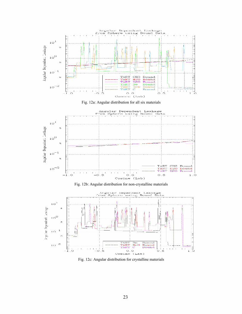
Fig. 12a: Angular distribution for all six materials

Fig. 12b: Angular distribution for non-crystalline materials

Fig. 12c: Angular distribution for crystalline materials

23

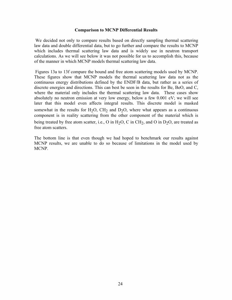
Comparison to MCNP Differential Results We decided not only to compare results based on directly sampling thermal scattering law data and double differential data, but to go further and compare the results to MCNP which includes thermal scattering law data and is widely use in neutron transport calculations. As we will see below it was not possible for us to accomplish this, because of the manner in which MCNP models thermal scattering law data. Figures 13a to 13f compare the bound and free atom scattering models used by MCNP. These figures show that MCNP models the thermal scattering law data not as the continuous energy distributions defined by the ENDF/B data, but rather as a series of discrete energies and directions. This can best be seen in the results for Be, BeO, and C, where the material only includes the thermal scattering law data. These cases show absolutely no neutron emission at very low energy, below a few 0.001 eV; we will see later that this model even affects integral results. This discrete model is masked somewhat in the results for H2O, CH2 and D2O, where what appears as a continuous component is in reality scattering from the other component of the material which is being treated by free atom scatter, i.e., O in H2O, C in CH2, and O in D2O, are treated as free atom scatters. The bottom line is that even though we had hoped to benchmark our results against MCNP results, we are unable to do so because of limitations in the model used by MCNP.

24

Fig. 13a: Comparison of H in H2O scattering using MCNP’s model

Fig. 13b: Comparison of H in CH2 scattering using MCNP’s model

25

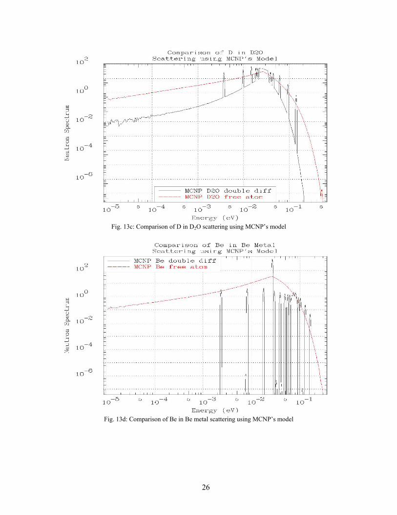
Fig. 13c: Comparison of D in D2O scattering using MCNP’s model

Fig. 13d: Comparison of Be in Be metal scattering using MCNP’s model

26

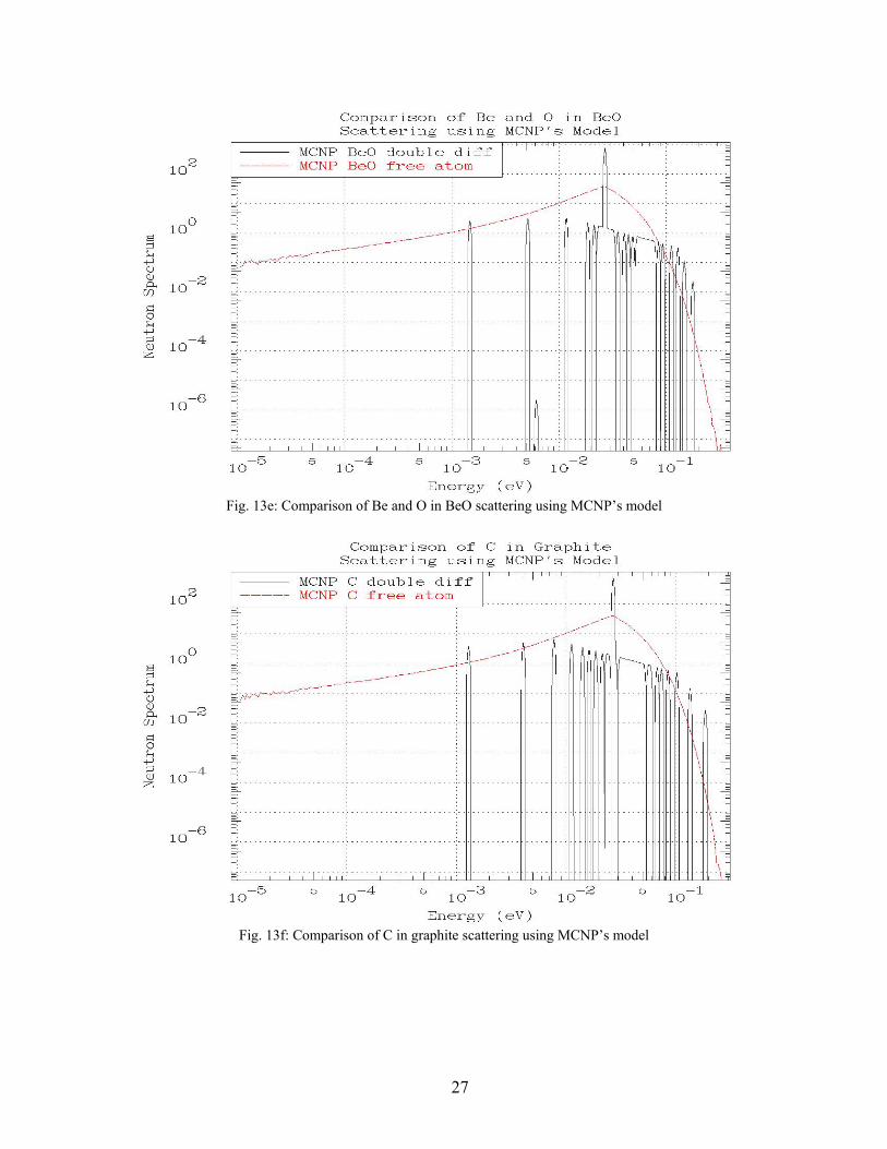
Fig. 13e: Comparison of Be and O in BeO scattering using MCNP’s model

Fig. 13f: Comparison of C in graphite scattering using MCNP’s model

27

Integral Test Problem For our integral results we examine slowing down spectra leaking from a sphere of each material. Here we are interested in both the energy and time distributions. These may sound like simple, somewhat theoretical problems, but in fact they correspond to what one encounters when these materials are used in any actual application. 1) For our integral test problem we use a sphere of a radius selected to insure that most neutrons thermalize before they leak from the sphere. The following radii were selected as adequate for this purpose , CH2: 10 cm H2O: 10 cm D2O: 20 cm Be Metal: 20 cm BeO: 20 cm C: 30 cm 2) A point source is located at the center of the sphere. 3) The neutron source is an isotropic, generic fission spectrum (results are very insensitive to the details of the fission spectrum used). The energy spectrum of neutrons “leaking” from the sphere are tallied in 50 energy bins per energy decade, equally spaced in the log of the energy, between 10

-5 eV and 20

MeV. The time dependent spectrum is tallied in 1 microsecond intervals from 1 to 1000 microseconds.

28

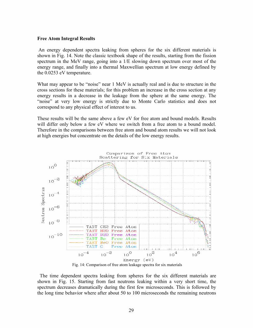
Free Atom Integral Results An energy dependent spectra leaking from spheres for the six different materials is shown in Fig. 14. Note the classic textbook shape of the results, starting from the fission spectrum in the MeV range, going into a 1/E slowing down spectrum over most of the energy range, and finally into a thermal Maxwellian spectrum at low energy defined by the 0.0253 eV temperature. What may appear to be “noise” near 1 MeV is actually real and is due to structure in the cross sections for these materials; for this problem an increase in the cross section at any energy results in a decrease in the leakage from the sphere at the same energy. The “noise” at very low energy is strictly due to Monte Carlo statistics and does not correspond to any physical effect of interest to us. These results will be the same above a few eV for free atom and bound models. Results will differ only below a few eV where we switch from a free atom to a bound model. Therefore in the comparisons between free atom and bound atom results we will not look at high energies but concentrate on the details of the low energy results.

Fig. 14: Comparison of free atom leakage spectra for six materials

The time dependent spectra leaking from spheres for the six different materials are shown in Fig. 15. Starting from fast neutrons leaking within a very short time, the spectrum decreases dramatically during the first few microseconds. This is followed by the long time behavior where after about 50 to 100 microseconds the remaining neutrons

29

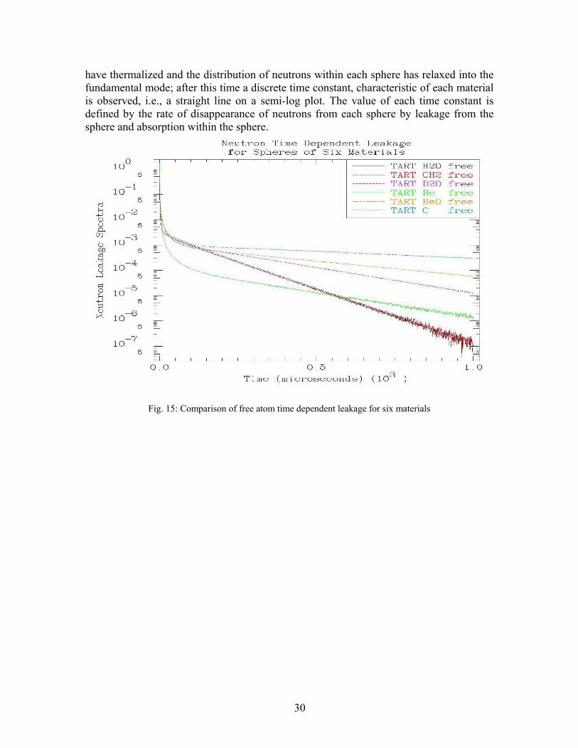
have thermalized and the distribution of neutrons within each sphere has relaxed into the fundamental mode; after this time a discrete time constant, characteristic of each material is observed, i.e., a straight line on a semi-log plot. The value of each time constant is defined by the rate of disappearance of neutrons from each sphere by leakage from the sphere and absorption within the sphere.

Fig. 15: Comparison of free atom time dependent leakage for six materials

30

Bound Integral Comparisons In our next set of integral comparisons we compare the spectrum based on directly sampling the thermal scattering law data to the results obtained sampling an “equivalent” double-differential representation of the data. For comparison we also include the free atom results. These comparisons show the difference between free atom and bound models. First note the common behavior between all of the spectra, which shift from a 1/E slowing down spectra to a thermal shape near a few tenths of an eV; this is true for both free and bound scatter. Only at low energies do the spectra begin to differ. For H bound in H2O (fig. 16a) and CH2 (fig. 16b) the spectra are similar over the entire energy range, and at lower energies there is roughly a factor of two difference between the free and bound spectra. In contrast, for D bound in D2O (fig.16c) there is much less

difference between the free and bound results. For the non-crystalline materials, H2O,

CH2 and D2O the bound spectra are smoothly varying over the entire energy range. For the crystalline materials, Be in Be Metal (fig. 16d), Be and O in BeO (fig. 16e) and C in graphite (fig. 16f), the spectra shows the effect of the Bragg edges. In these example problems we are examining the neutron leakage from the spheres. In these cases as we proceed from higher to lower energy, a decrease in the cross section, as occurs as the Bragg edges, results in an increase in the leakage, which is exactly what we see in the below spectra.

31

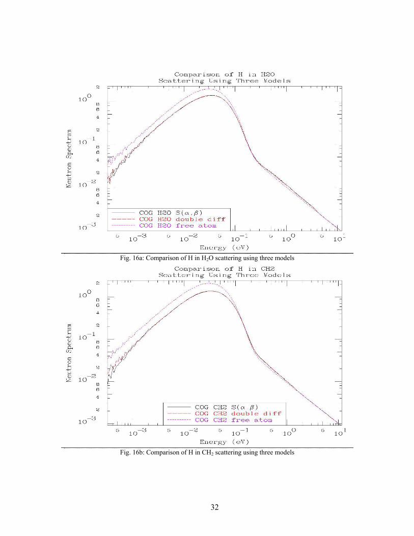
Fig. 16a: Comparison of H in H2O scattering using three models

Fig. 16b: Comparison of H in CH2 scattering using three models

32

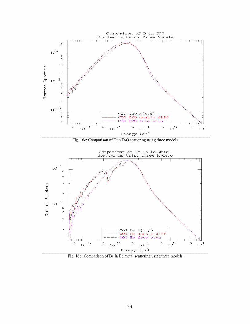
Fig. 16c: Comparison of D in D2O scattering using three models

33

Fig. 16d: Comparison of Be in Be metal scattering using three models

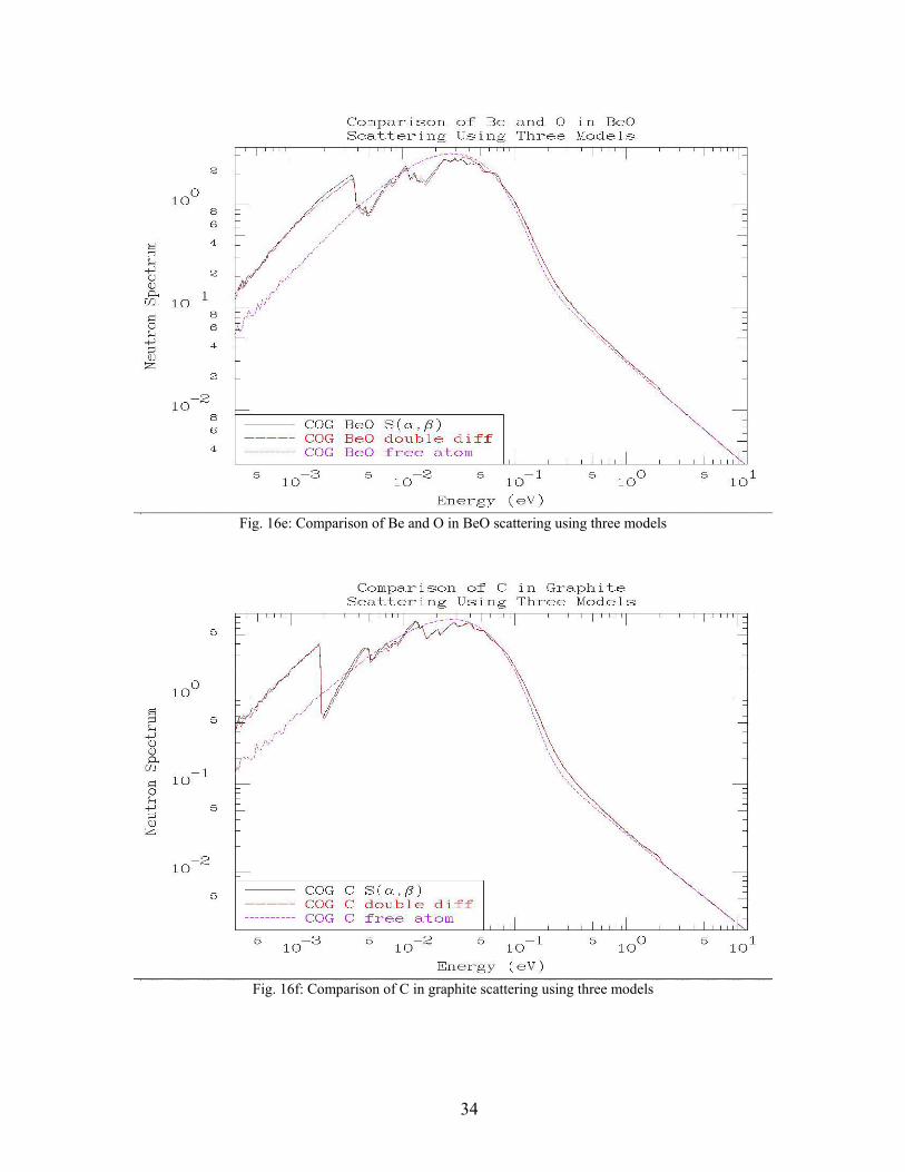
Fig. 16e: Comparison of Be and O in BeO scattering using three models

Fig. 16f: Comparison of C in graphite scattering using three models

34

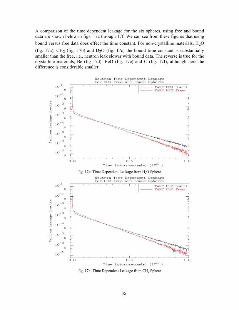
A comparison of the time dependent leakage for the six spheres, using free and bound data are shown below in figs. 17a through 17f. We can see from these figures that using bound versus free data does effect the time constant. For non-crystalline materials, H2O (fig. 17a), CH2 (fig. 17b) and D2O (fig. 17c) the bound time constant is substantially smaller than the free, i.e., neutron leak slower with bound data. The reverse is true for the crystalline materials, Be (fig 17d), BeO (fig. 17e) and C (fig. 17f), although here the difference is considerable smaller.

fig. 17a: Time Dependent Leakage from H2O Sphere

fig. 17b: Time Dependent Leakage from CH2 Sphere

35

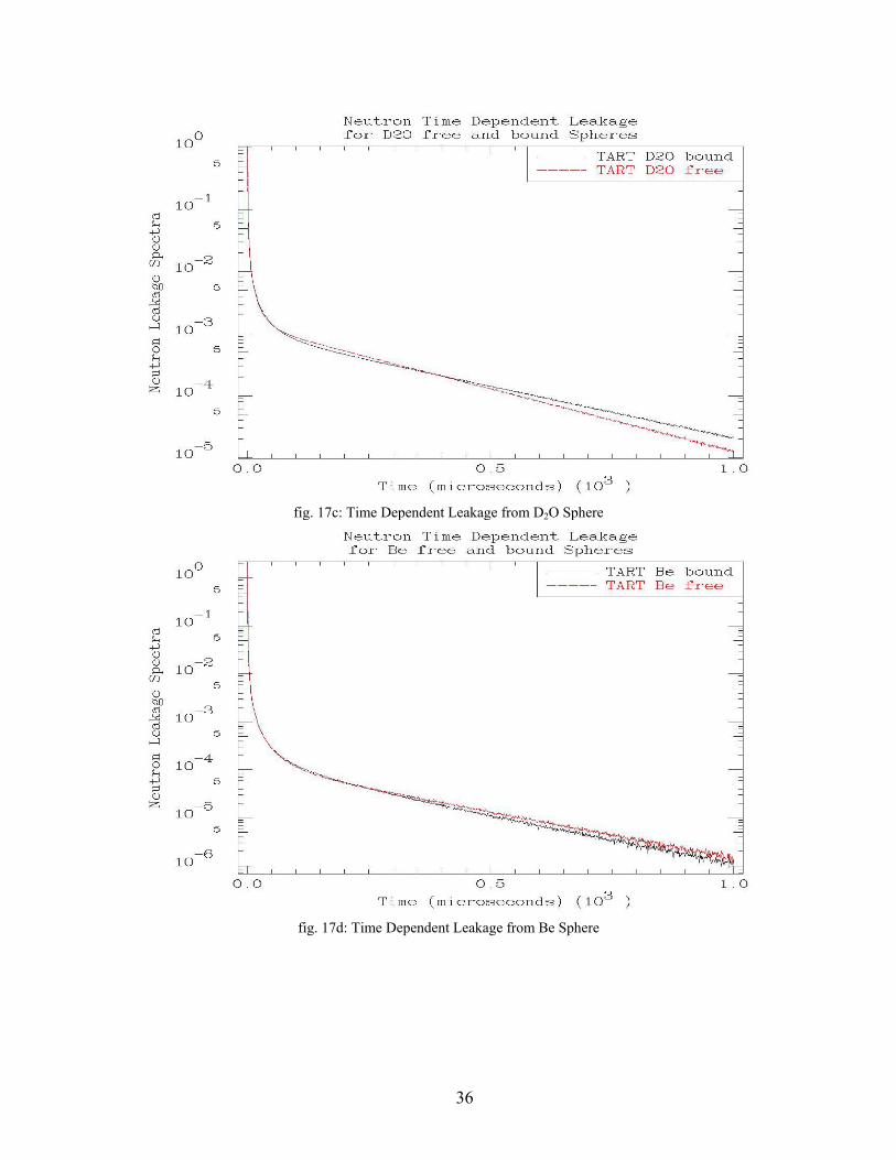
fig. 17c: Time Dependent Leakage from D2O Sphere

fig. 17d: Time Dependent Leakage from Be Sphere

36

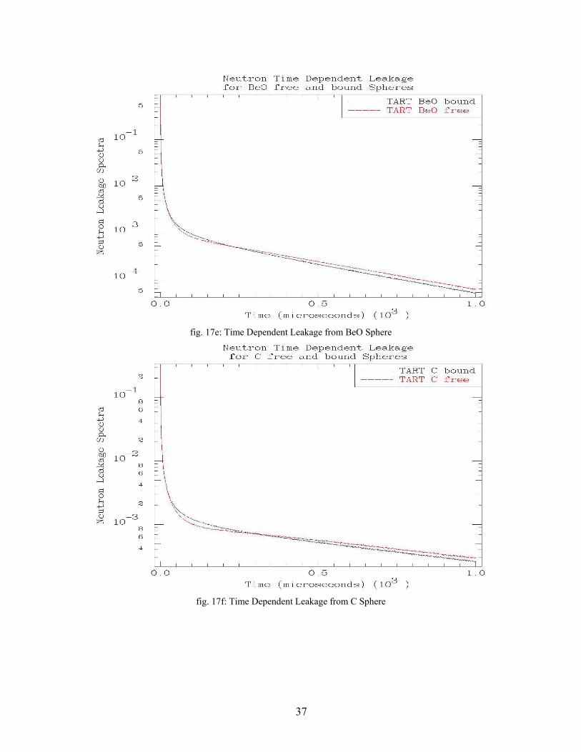
fig. 17e: Time Dependent Leakage from BeO Sphere

fig. 17f: Time Dependent Leakage from C Sphere

37

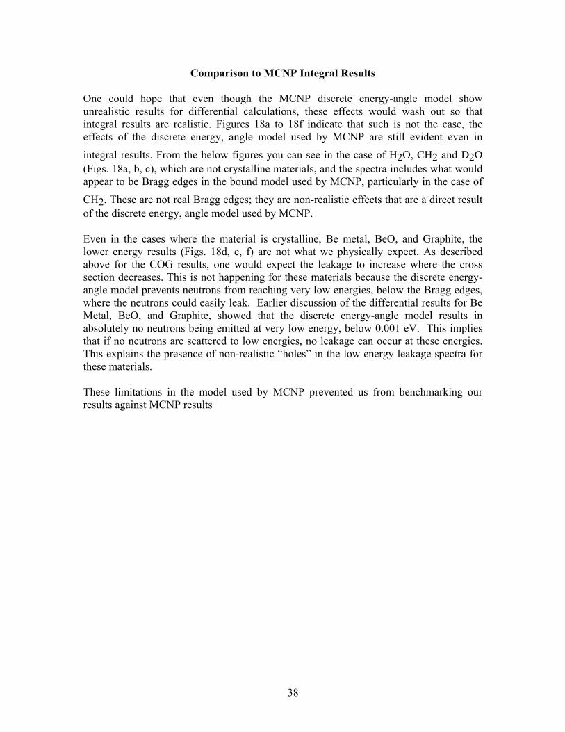
Comparison to MCNP Integral Results One could hope that even though the MCNP discrete energy-angle model show unrealistic results for differential calculations, these effects would wash out so that integral results are realistic. Figures 18a to 18f indicate that such is not the case, the effects of the discrete energy, angle model used by MCNP are still evident even in integral results. From the below figures you can see in the case of H2O, CH2 and D2O (Figs. 18a, b, c), which are not crystalline materials, and the spectra includes what would appear to be Bragg edges in the bound model used by MCNP, particularly in the case of CH2. These are not real Bragg edges; they are non-realistic effects that are a direct result of the discrete energy, angle model used by MCNP. Even in the cases where the material is crystalline, Be metal, BeO, and Graphite, the lower energy results (Figs. 18d, e, f) are not what we physically expect. As described above for the COG results, one would expect the leakage to increase where the cross section decreases. This is not happening for these materials because the discrete energy-angle model prevents neutrons from reaching very low energies, below the Bragg edges, where the neutrons could easily leak. Earlier discussion of the differential results for Be Metal, BeO, and Graphite, showed that the discrete energy-angle model results in absolutely no neutrons being emitted at very low energy, below 0.001 eV. This implies that if no neutrons are scattered to low energies, no leakage can occur at these energies. This explains the presence of non-realistic “holes” in the low energy leakage spectra for these materials. These limitations in the model used by MCNP prevented us from benchmarking our results against MCNP results

38

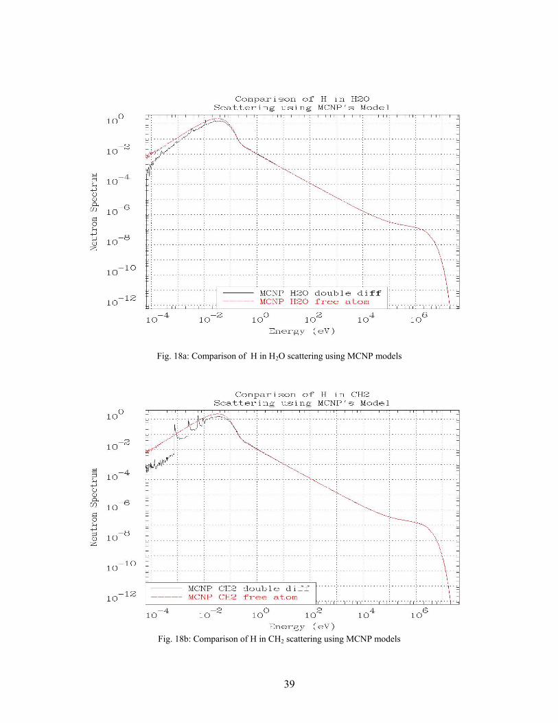
Fig. 18a: Comparison of H in H2O scattering using MCNP models

Fig. 18b: Comparison of H in CH2 scattering using MCNP models

39

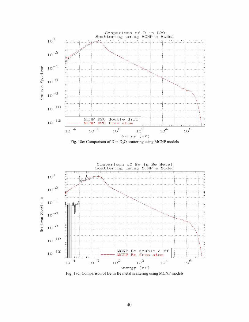
Fig. 18c: Comparison of D in D2O scattering using MCNP models

Fig. 18d: Comparison of Be in Be metal scattering using MCNP models

40

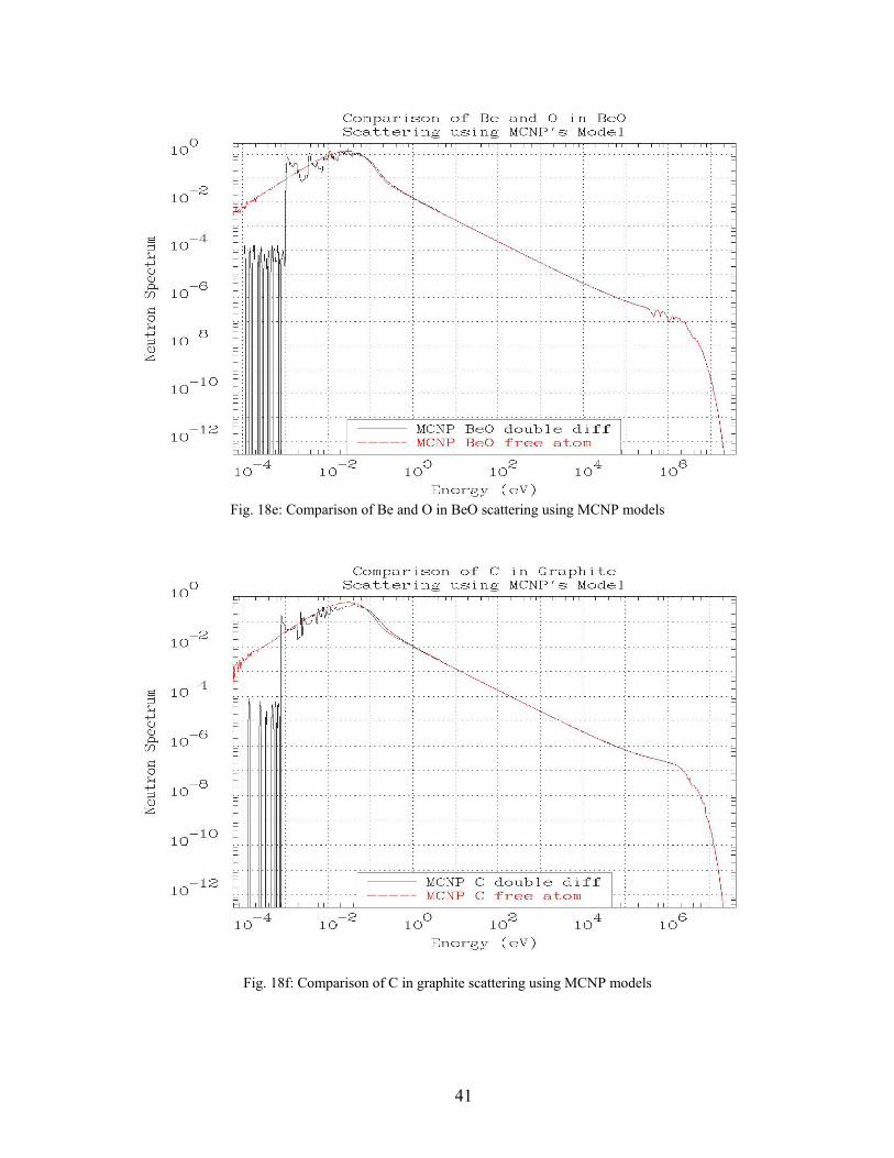
Fig. 18e: Comparison of Be and O in BeO scattering using MCNP models

Fig. 18f: Comparison of C in graphite scattering using MCNP models

41

Critical Assemblies

The last set of comparisons are TART results for critical assembly integral parameters using bound and free atom data. The following table of 50 U

235 and U

233 fueled thermal

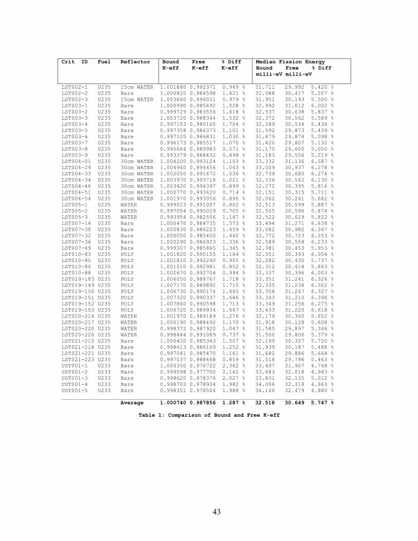
critical assemblies were all taken from the “International Handbook of Evaluated Criticality Safety Benchmark Experiments”, September 2002 Edition [9]. In table 1, below, the Crit ID (Criticality ID) for each assembly is an abbreviated form of that used in the handbook, specifically, LST = LEU SOL THERM = Low Enriched Uranium, Solution, Thermal Spectrum UST = U233 SOL THERM = U

233, Solution, Thermal Spectrum

From table 1, below, it can be seen that in every single one of the 50 cases the bound K-eff is higher than the free K-eff, with an average increase of about 1.3 %. The biggest increases are for all of the U

233 fueled assemblies, where the bound values of K-eff are

all very close to unity. Much of this increase in K-eff can be attributed to a significantly higher median fission energy using bound data. Again, in every single one of the 50 cases in table 1 the median fission energy is higher using bound data; in most cases the increase is 4 to 6 %, and on average it is increased by 5.7 %.

42

Crit ID Fuel Reflector Bound Free % Diff

K-eff K-eff K-eff Median Fission Energy Bound Free % Diff milli-eV milli-eV

LST002-1 U235 15cm WATER 1.001880 0.992371 0.949 % 31.711 29.992 5.420 % LST002-2 U235 Bare 1.000820 0.984598 1.621 % 32.088 30.417 5.207 % LST002-3 U235 15cm WATER 1.003860 0.994031 0.979 % 31.951 30.193 5.500 % LST003-1 U235 Bare 1.000990 0.985692 1.528 % 32.992 31.012 6.002 % LST003-2 U235 Bare 0.999729 0.983556 1.618 % 32.537 30.638 5.837 % LST003-3 U235 Bare 1.003720 0.988344 1.532 % 32.372 30.562 5.589 % LST003-4 U235 Bare 0.997153 0.980165 1.704 % 32.289 30.534 5.436 % LST003-5 U235 Bare 0.997358 0.986373 1.101 % 31.592 29.873 5.439 % LST003-6 U235 Bare 0.997105 0.986831 1.030 % 31.479 29.874 5.098 % LST003-7 U235 Bare 0.996173 0.985517 1.070 % 31.420 29.807 5.132 % LST003-8 U235 Bare 0.995664 0.989983 0.571 % 31.175 29.600 5.050 % LST003-9 U235 Bare 0.993379 0.988432 0.498 % 31.183 29.556 5.219 % LST004-01 U235 30cm WATER 1.004200 0.993124 1.103 % 33.332 31.136 6.587 % LST004-29 U235 30cm WATER 1.004940 0.994456 1.043 % 33.009 30.937 6.278 % LST004-33 U235 30cm WATER 1.002050 0.991672 1.036 % 32.739 30.685 6.274 % LST004-34 U235 30cm WATER 1.003970 0.993718 1.021 % 32.536 30.542 6.130 % LST004-46 U235 30cm WATER 1.003420 0.994397 0.899 % 32.272 30.395 5.816 % LST004-51 U235 30cm WATER 1.000770 0.993620 0.714 % 32.151 30.315 5.711 % LST004-54 U235 30cm WATER 1.001970 0.993056 0.890 % 32.062 30.241 5.682 % LST005-1 U235 WATER 0.999023 0.991007 0.802 % 32.513 30.599 5.887 % LST005-2 U235 WATER 0.997054 0.990029 0.705 % 32.505 30.596 5.874 % LST005-3 U235 WATER 0.993954 0.982556 1.147 % 32.522 30.629 5.822 % LST007-14 U235 Bare 1.000470 0.984735 1.573 % 33.494 31.271 6.638 % LST007-30 U235 Bare 1.000830 0.986223 1.459 % 33.082 30.982 6.347 % LST007-32 U235 Bare 1.000050 0.985450 1.460 % 32.772 30.723 6.253 % LST007-36 U235 Bare 1.000290 0.986923 1.336 % 32.589 30.558 6.233 % LST007-49 U235 Bare 0.999307 0.985865 1.345 % 32.381 30.453 5.953 % LST010-83 U235 POLY 1.001820 0.990155 1.164 % 32.351 30.393 6.054 % LST010-85 U235 POLY 1.001810 0.992240 0.955 % 32.282 30.430 5.737 % LST010-86 U235 POLY 1.001510 0.992981 0.852 % 32.312 30.418 5.863 % LST010-88 U235 POLY 1.002670 0.992706 0.994 % 32.337 30.396 6.003 % LST019-183 U235 POLY 1.006050 0.988767 1.718 % 33.351 31.241 6.326 % LST019-149 U235 POLY 1.007170 0.989892 1.715 % 33.335 31.234 6.302 % LST019-150 U235 POLY 1.006730 0.990174 1.645 % 33.358 31.247 6.327 % LST019-151 U235 POLY 1.007320 0.990337 1.686 % 33.343 31.210 6.398 % LST019-152 U235 POLY 1.007860 0.990598 1.713 % 33.349 31.256 6.275 % LST019-153 U235 POLY 1.006720 0.989934 1.667 % 33.433 31.220 6.618 % LST020-216 U235 WATER 1.001970 0.989189 1.276 % 32.179 30.360 5.652 % LST020-217 U235 WATER 1.000190 0.988492 1.170 % 31.918 30.128 5.608 % LST020-220 U235 WATER 0.998372 0.987920 1.047 % 31.585 29.897 5.346 % LST020-226 U235 WATER 0.998444 0.991089 0.737 % 31.500 29.806 5.379 % LST021-215 U235 Bare 1.000420 0.985343 1.507 % 32.199 30.357 5.720 % LST021-218 U235 Bare 0.998613 0.986109 1.252 % 31.939 30.187 5.488 % LST021-221 U235 Bare 0.997041 0.985470 1.161 % 31.682 29.886 5.668 % LST021-223 U235 Bare 0.997037 0.988468 0.859 % 31.518 29.796 5.463 % UST001-1 U233 Bare 1.000350 0.976722 2.362 % 33.497 31.907 4.748 % UST001-2 U233 Bare 0.999098 0.977700 2.142 % 33.683 32.018 4.943 % UST001-3 U233 Bare 0.998620 0.978376 2.027 % 33.831 32.135 5.012 % UST001-4 U233 Bare 0.998703 0.978904 1.982 % 34.006 32.318 4.963 % UST001-5 U233 Bare 0.998351 0.978504 1.988 % 34.146 32.479 4.880 % ___________________________________________________________________________________ Average 1.000740 0.987856 1.287 % 32.518 30.649 5.747 %

Table 1: Comparison of Bound and Free K-eff

43

Conclusions

Recently we implemented the ENDF/B-VI thermal scattering law data in our neutron transport codes COG and TART. Our objective was to convert the existing ENDF/B data into double differential form, in the Livermore ENDL format, so that it would be available for use in any neutron transport code, be it a Monte Carlo or deterministic code. This was approached as a multi-step project. The first step was to develop methods to directly use the thermal scattering law data in our Monte Carlo codes. The next step was to convert the data to double-differential form. The last step was to verify that the results obtained using the data directly are essentially the same as the results obtained using the double differential data. Part of the planned verification was intended to insure that the data as finally implemented in our COG and TART codes gave the same answers as the widely used MCNP code, which includes this thermal scattering law data. However, the present work has uncovered limitations in the treatment that MCNP uses for thermal scattering data, giving rise to unphysical results. Consequently, calculations of COG and TART results at thermal energies are not expect to agree with MCNP results. Table 1 results for thermal critical assemblies illustrate how important thermal scattering law data is in our applications. Again, note that in every single case the bound results are higher than the free results, and in every single case the bound results are closer to the value of unity that we expect.

Where do we go from here? So far we have investigated the use of thermal scattering data for six materials (H2O, D2O, CH2, Be, BeO and C) at room temperature. We intend to extend this work to more materials, for continuous variation in temperature. This may require use of so called synthetic scattering kernels, Debye effective temperature, or other models. We would like to obtain results for our test problems for other neutron transport codes. These comparisons among different codes allow us to pinpoint limitations in the physical models used, as occurred in the case with the MCNP code using thermal scattering law data. We hope that the limitations in the MCNP model will be corrected leading to improvements in MCNP. It is planned that additional or improved results will be compared with COG and TART as well with other transport codes and updated results will be published in a revision of this report.

44

References

[1] “New Thermal Neutron Scattering Files for ENDF/B-VI Release 2”, Los Alamos National Laboratory, March 1994, by R.E. MacFarlane [2] COG: A Multiparticle Monte Carlo Transport Code, Fifth Edition (Sept. 2002), Lawrence Livermore National Laboratory, (report #) and (authors) [3] “TART 2002: A Coupled Neutron-Photon 3-D, Combinatorial Geometry Time Dependent Monte Carlo Transport Code," Lawrence Livermore National Laboratory, UCRL-ID-126455, Rev. 4, November, 2002, by D.E. Cullen [4] “The LLL Evaluated Nuclear Data Library (ENDL): Evaluation Techniques, Reaction Index, and Description of Individual Evaluations”, UCRL-50400, Vol. 15, Part A, Sept. 1975, Lawrence Livermore National Laboratory, by R. J. Howerton, et. al, [5] MCNP4C2: A General Monte Carlo N-Particle Transport Code, Version 4C, Los Alamos National Laboratory, LA-13709-M, 2002, ed. J.F. Briesmeister [6] “Data Formats and Procedures for the Evaluated Nuclear Data File, ENDF-6”, ENDF-102, Brookhaven National Laboratory, April 2001, ed. V. McLane [7]“A Temperature Dependent ENDF/B-VI, Release 8 Cross Section Library”, Lawrence Livermore National Laboratory, UCRL-ID-127776, Rev. 2, May 2003, by D.E. Cullen [8] "Exact Doppler Broadening of Tabulated Cross Sections," Nuclear Science and Engineering 60, p. 199, 1975, by D.E. Cullen and C.R. Weisbin [9] “International Handbook of Evaluated Criticality Safety Benchmark Experiments”, Idaho National Engineering and Environmental Laboratory, September 2002 Edition. Editor, J. Blair Briggs

45

University of CaliforniaLawrence Livermore National LaboratoryTechnical Information DepartmentLivermore, CA 94551