HAL Id: insu-00279845https://hal-insu.archives-ouvertes.fr/insu-00279845

Submitted on 15 May 2008

HAL is a multi-disciplinary open accessarchive for the deposit and dissemination of sci-entific research documents, whether they are pub-lished or not. The documents may come fromteaching and research institutions in France orabroad, or from public or private research centers.

L’archive ouverte pluridisciplinaire HAL, estdestinée au dépôt et à la diffusion de documentsscientifiques de niveau recherche, publiés ou non,émanant des établissements d’enseignement et derecherche français ou étrangers, des laboratoirespublics ou privés.

Thermal regime of the NW shelf of the Gulf of Mexico.1) Thermal and pressure fields

Laurent Husson, Pierre Henry, Xavier Le Pichon

To cite this version:Laurent Husson, Pierre Henry, Xavier Le Pichon. Thermal regime of the NW shelf of the Gulf ofMexico. 1) Thermal and pressure fields. bulletin de la societe geologique, 2008, 179 (2), pp.129-137.�insu-00279845�

Thermal regime of the NW shelf of the Gulf of Mexico.

1) Thermal and pressure fields

Bulletin de la Société Géologique de France, in press

Laurent Husson, a,b Pierre Henry a, Xavier Le Pichon a

a Collège de France, Chaire de Géodynamique, Europôle de l’Arbois, 13545 Aix-en-

Provence, France. henry@cdf.u-3mrs.fr (P. Henry); lepichon@cdf.u-3mrs.fr (X. Le Pichon)

b Géosciences Rennes, UMR CNRS 6118, Université de Rennes-1, Campus de Beaulieu,

35042 Rennes Cedex, FRANCE. laurent.husson@univ-rennes1.fr (L. Husson)

Abstract

The thermal field of the Gulf of Mexico (GoM) is analyzed from a comprehensive temperature-depth

database of about 8500 Bottom Hole Temperatures and Reservoir Temperatures. Our stochastic

analysis reveals a widespread, systematic sharp thermal gradient increase between 2500 and 4000 m.

The analysis of the pressure regime indicates a systematic correlation between the pressure and

temperature fields.

Keywords: Gulf of Mexico, geotherm, pressure.

Régime thermique de la marge nord-ouest du Golfe du Mexique.

1) Champs de temperature et de pression.

Résumé

Le régime thermique du Golfe du Mexique (GoM – Gulf of Mexico) est examiné à partir d’une base de

8500 données de températures de fond de puit et de températures de réservoir. Notre analyse

stochastique révèle une augmentation brutale systématique et régionale du gradient de température

entre 2500 et 4000 m. L’analyse du régime de pression montre une correlation entre les champs de

température et de pression.

Mots-clefs: Golfe du Mexique, géotherme, pression.

1. Introduction

Although the NW margin of the Gulf of Mexico (GoM) has been the locus of myriads of geological

studies, both its thermal and tectonic structures remain unclear. Even the geometry of the thermal field

is still controversial due to the high complexity of the tectonic and sedimentary processes but also due

to the lack of a coherent analysis at the scale of the entire shelf, as most studies have industrial aims

and focus on reservoir scales. As a first step toward understanding the thermal regime of the NW shelf

of the GoM, we performed a joint analysis of the thermal and pressure fields of the Louisiana and

Texas shelf basins to characterize the general thermal structure, examine its possible relationship with

the tectonic structure, and discuss the processes that may be responsible for such a complexity.

Thermal modeling is a complementary analysis that is given in a companion paper [Husson et al.,

submitted to B.S.G.F.].

1.1. Geological setting

The NW margin of the GoM is characterized by a large Oligo-Miocene detachment on which a series

of NE-SW to E-W trending normal faults branch (Fig. 1). Among them, the Wilcox and Corsair Fault

Zones (WFZ and CFZ) display offsets of more than 20 km and run across the whole width of Texas.

Extension on these fault systems is generally attributed to gravitational collapse toward the Gulf on a

Cenozoic detachment [Pindell & Dewey, 1982; Diegel et al., 1995; Hall, 2002]. The bulk strain is

assumed to have been transmitted at the base of the slope where it is accommodated by the Perdido and

Mississippi fan fold belts. The structural style of the deep shelf drastically differs as it is mostly

characterized by the abundance of salt canopies; only small quantities of salt remain in the proximal

shelf. The Rio Bravo marks the location of a left-lateral Tertiary fault which separates the Texan and

Mexican units [Russell et Snelson, 1994]. We identified six tectono-stratigraphic provinces (Fig.1) that

we will consider in order to explore their relationships with the thermal field, namely the CFZ and its

onshore analogue the WFZ, the intermediate zone in between (Intermediate Texas Zone ITZ), the

north-west of the WFZ (North West Wilcox, NWW), Louisiana (LA), and the N. Mexican Burgos

basin (BUR), subdivided in East and West (EBUR and WBUR, respectively). Additional support for

this division is given by their thermal state (see section 2.2).

1.2. Temperature data sets

A compilation of ~2000 offshore Reservoir Temperature data (RT) and ~6500 both offshore and

onshore Bottom Hole Temperature data (BHT) of industrial origin have been used to characterize the

thermal regime (Fig.1). The complete databases are provided as electronic supplements (Tables E1 and

E2). RT provide direct measures of the temperature at depth and are fairly reliable, since they give the

equilibrium temperature. On the contrary, many BHT data were acquired before thermal equilibrium

was reached. Empirical [e.g., Bullard, 1947; Horner, 1951]) and statistical [e.g., Deming& Chapman,

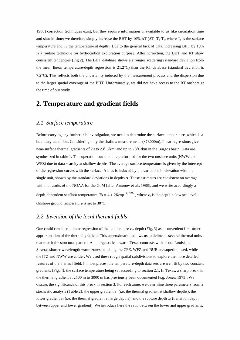
1988] correction techniques exist, but they require information unavailable to us like circulation time

and shut-in-time; we therefore simply increase the BHT by 10% T ( T=Tb-Ts, where Ts is the surface

temperature and Tb the temperature at depth). Due to the general lack of data, increasing BHT by 10%

is a routine technique for hydrocarbon exploration purpose. After correction, the BHT and RT show

consistent tendencies (Fig.2). The BHT database shows a stronger scattering (standard deviation from

the mean linear temperature-depth regression is 21.2°C) than the RT database (standard deviation is

7.2°C). This reflects both the uncertainty induced by the measurement process and the dispersion due

to the larger spatial coverage of the BHT. Unfortunately, we did not have access to the RT onshore at

the time of our study.

2. Temperature and gradient fields

2.1. Surface temperature

Before carrying any further this investigation, we need to determine the surface temperature, which is a

boundary condition. Considering only the shallow measurements (< 3000m), linear regressions give

near-surface thermal gradients of 20 to 23°C/km, and up to 28°C/km in the Burgos basin. Data are

synthesized in table 1. This operation could not be performed for the two onshore units (NWW and

WFZ) due to data scarcity at shallow depths. The average surface temperature is given by the intercept

of the regression curves with the surface. A bias is induced by the variations in elevation within a

single unit, shown by the standard deviations in depths . These estimates are consistent on average

with the results of the NOAA for the GoM [after Antonov et al., 1988], and we write accordingly a

depth-dependent seafloor temperature Ts = 4 + 26expz

s/300

, where zs is the depth below sea level.

Onshore ground temperature is set to 30°C.

2.2. Inversion of the local thermal fields

One could consider a linear regression of the temperature vs. depth (Fig. 3) as a convenient first-order

approximation of the thermal gradient. This approximation allows us to delineate several thermal units

that match the structural pattern. At a large scale, a warm Texas contrasts with a cool Louisiana.

Several shorter wavelength warm zones matching the CFZ, WFZ and BUR are superimposed, while

the ITZ and NWW are colder. We used these rough spatial subdivisions to explore the more detailed

features of the thermal field. In most places, the temperature-depth data sets are well fit by two constant

gradients (Fig. 4), the surface temperature being set according to section 2.1. In Texas, a sharp break in

the thermal gradient at 2500 m to 3000 m has previously been documented [e.g. Jones, 1975]. We

discuss the significance of this break in section 3. For each zone, we determine three parameters from a

stochastic analysis (Table 2): the upper gradient a1 (i.e. the thermal gradient at shallow depths), the

lower gradient a2 (i.e. the thermal gradient at large depths), and the rupture depth z0 (transition depth

between upper and lower gradient). We introduce here the ratio between the lower and upper gradients.

For WFZ, ITZ, CFZ and LA, a composite two-gradients fit has a considerably better fit than that given

by a single linear regression,or even a quadratic regression (leaving the possibility of a continuous

change rather than a discrete change in temperature gradient). Error minimization has been performed

using both L1 (sum of errors) and L2 (mean square of errors) norms. We eliminated outliers until

norms L1 and L2 gave consistent results. Only 20 outlying values had to be withdrawn. We also

compared regressions obtained using RT and BHT data separately. Once the rupture depth in the

temperature profile is fixed, the upper gradients from RT and BHT are in good agreement. We

conclude that the sharp downward increase in the temperature profiles is a real feature.

The rupture depth in the thermal gradient occurs at about 2500 m for WFZ, ITZ, and CFZ. In NWW,

the rupture depth of the gradient is poorly constrained. As the geological setting does not differ much

from that of the neighboring WFZ, we adopt the same break in gradient depth in NWW as in the WFZ.

In LA, the gradient rupture exists too, but at a greater depth than in the other zones (4250 m). For LA,

because the rupture depth is large, the high gradient is deep and the temperature is low at all depths. In

BUR, not enough data are available at large depths and only a single regression can be performed.

Maximum and minimum upper section gradients are found respectively in BUR (29 °C /km for W

BUR and 27 °C /km for W BUR), and ITZ (18.9 °C/km), respectively, making the upper gradient cold

everywhere except in BUR.

2.3. Three-dimensional mapping of the thermal field with depth

We use the results of the previous analysis to assess the 3D temperature field of the GoM from all

available BHT and RT data. The previous analysis gives the mean tendency of the subsurface thermal

gradient, where the geotherm T(z) writes

T(z)=Ts+a1z, (z<z0)

T(z)=Ts+a1z+a2(z-z0), (z>z0) (1)

Assuming that the previously calculated values for z0 hold anywhere within a given zone, we then

extrapolate the general laws to individual data i. We keep a constant ratio Nu=a2/a1 and calculate for

each data a new coefficient bi so that the temperature evolves with depth like

T(z)i=Ts+b ia1z, (z<z0)

T(z) i =Ts+b ia1z+b ia2(z-z0), (z>z0) (2)

We then filtered (see appendix A1) and mapped the upper and lower thermal gradients by interpolating

bia1 and bia2, respectively. The upper gradient (Fig. 5a) peaks in the WFZ and CFZ (up to 28-30°C/km)

but remains fairly homogeneous (~19 to 25°C/km). BUR remains the warmest zone at a large scale

(~30°C/km). At depth (Fig. 5b), the gradient increases everywhere between ~34 and 39°C/km (we do

not extrapolate the results to the deep gradient south of 26° latitude because of the lack of data). Such

gradient increase is an unexpected feature since the thermal regimes of sedimentary basins are above

all controlled by the conductivity, which increases with compaction. Notice the strong discrepancy

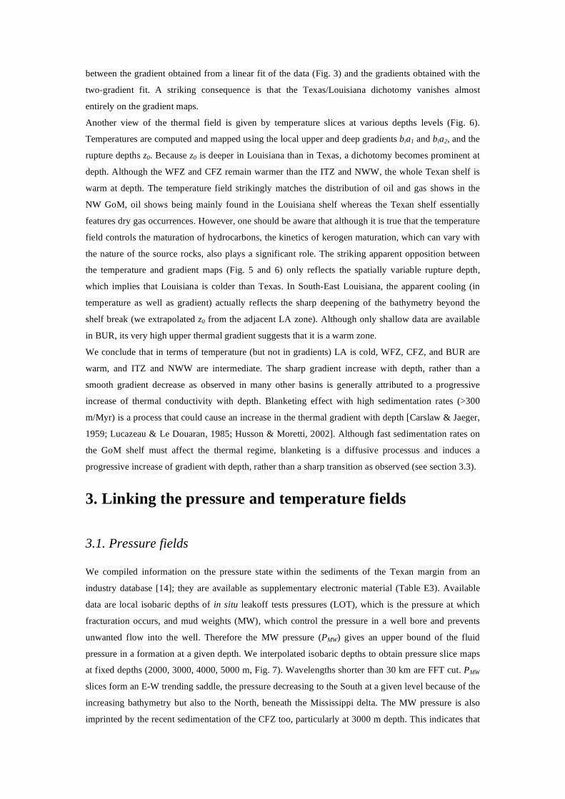
between the gradient obtained from a linear fit of the data (Fig. 3) and the gradients obtained with the

two-gradient fit. A striking consequence is that the Texas/Louisiana dichotomy vanishes almost

entirely on the gradient maps.

Another view of the thermal field is given by temperature slices at various depths levels (Fig. 6).

Temperatures are computed and mapped using the local upper and deep gradients bia1 and bia2, and the

rupture depths z0. Because z0 is deeper in Louisiana than in Texas, a dichotomy becomes prominent at

depth. Although the WFZ and CFZ remain warmer than the ITZ and NWW, the whole Texan shelf is

warm at depth. The temperature field strikingly matches the distribution of oil and gas shows in the

NW GoM, oil shows being mainly found in the Louisiana shelf whereas the Texan shelf essentially

features dry gas occurrences. However, one should be aware that although it is true that the temperature

field controls the maturation of hydrocarbons, the kinetics of kerogen maturation, which can vary with

the nature of the source rocks, also plays a significant role. The striking apparent opposition between

the temperature and gradient maps (Fig. 5 and 6) only reflects the spatially variable rupture depth,

which implies that Louisiana is colder than Texas. In South-East Louisiana, the apparent cooling (in

temperature as well as gradient) actually reflects the sharp deepening of the bathymetry beyond the

shelf break (we extrapolated z0 from the adjacent LA zone). Although only shallow data are available

in BUR, its very high upper thermal gradient suggests that it is a warm zone.

We conclude that in terms of temperature (but not in gradients) LA is cold, WFZ, CFZ, and BUR are

warm, and ITZ and NWW are intermediate. The sharp gradient increase with depth, rather than a

smooth gradient decrease as observed in many other basins is generally attributed to a progressive

increase of thermal conductivity with depth. Blanketing effect with high sedimentation rates (>300

m/Myr) is a process that could cause an increase in the thermal gradient with depth [Carslaw & Jaeger,

1959; Lucazeau & Le Douaran, 1985; Husson & Moretti, 2002]. Although fast sedimentation rates on

the GoM shelf must affect the thermal regime, blanketing is a diffusive processus and induces a

progressive increase of gradient with depth, rather than a sharp transition as observed (see section 3.3).

3. Linking the pressure and temperature fields

3.1. Pressure fields

We compiled information on the pressure state within the sediments of the Texan margin from an

industry database [14]; they are available as supplementary electronic material (Table E3). Available

data are local isobaric depths of in situ leakoff tests pressures (LOT), which is the pressure at which

fracturation occurs, and mud weights (MW), which control the pressure in a well bore and prevents

unwanted flow into the well. Therefore the MW pressure (PMW) gives an upper bound of the fluid

pressure in a formation at a given depth. We interpolated isobaric depths to obtain pressure slice maps

at fixed depths (2000, 3000, 4000, 5000 m, Fig. 7). Wavelengths shorter than 30 km are FFT cut. PMW

slices form an E-W trending saddle, the pressure decreasing to the South at a given level because of the

increasing bathymetry but also to the North, beneath the Mississippi delta. The MW pressure is also

imprinted by the recent sedimentation of the CFZ too, particularly at 3000 m depth. This indicates that

the near hydrostatic pressure field extends deeper in fast sedimentation areas such as the CFZ and the

Mississippi delta than in other areas.

3.2. Overpressure

MW pressure PMW is necessarily between lithostatic Plit and hydrostatic Phyd pressures. The

overpressure state is quantified by the ratio R=(PMW - Phyd)/( Plit - Phyd). Details are given in appendix

A2. Fig. 8 shows interpolated overpressure slice maps. Wavelengths shorter than 30 km are FFT cut.

Within the NW GoM margin, the transition from low pressures (R<0.5) toward high pressures (R>0.5)

occurs between 2500 m and 3200 m in the Texan zone and at ~4500 m in Louisiana. The zones of

highest recent sedimentation rates (Mississippi delta and CFZ) match the zones of lower fluid pressure.

This is explained if these recent sediments have a high enough permeability and compact normally. A

spatial analysis confirms these observations.

The curves of Fig. 9 give the evolution of PMW, Plit, and Phyd with depth. We arbitrarily define a mean

curve, which runs through the mean depths at each reference pressure. The transition from almost

hydrostatic to high pressures occurs at lower depths in CFZ and ITZ (~3000 m) than in LA (~4200 m).

The lithostatic pressure is never reached in our interpolation and the measurements indicate that the

actual geopressure curve is asymptotic to the lithostatic gradient curves. This can be due to a choice of

too high a density for recent sediments. In that case, the transition depth should be slightly shallower

(~2500 in Texas and ~4000 in Louisiana).

On a general point of view, one should expect a thick recent sedimentary pile to be overpressured. The

fact that in the GoM shelf overpressure only appears at large depths suggests that the upper section is

highly permeable allowing for the water to be expelled at fast rates. The LOT pressures PLOT give the

pressure at which fracturing occurs in an open formation, i.e. the measured pressure is comparable to

the magnitude of the 3 component of the local stress tensor. Here we just want to mention that in the

NW of the GoM margin, PLOT (data in table E3) is rather close to the hydrostatic pressure at shallow

depths where the sedimentary pile is dominated by recent sediments. This implies that fracturation in

these areas occurs at shallow depth, and in turn indicates that fracture permeability is high in the recent

sediments of the GoM margin. The transition depth from nearly hydrostatically-pressured to high-P is

correlated with the thickness of Plio-Pleistocene sediments [Husson et al., submitted to B.S.G.F.;

Galloway et al., 2000].

3.3. Pressure, fluid flow, and temperature

The pressure field matches the thermal field described in section 2.2, since the thermal gradient shows

a sharp increase where the downward transition towards high pressures occurs. Indeed, this sharp

transition toward near-lithostatic pressure has been previously acknowledged onshore Texas [e.g.

Jones, 1975; Pfeiffer & Sharp, 1989; McKenna & Sharp, 1998; McKenna, 1997; Sharp et al., 2001].

The thermal field also match the thickness of the sedimentary cover, as previously acknowledged [for

instance in the NE GoM, Nagihara & Jones, 2005]. Our analysis shows that this setting is widespread

over the whole NW GoM margin.

The most obvious processes which can be invoked to explain the temperature gradient increase with

depth is the blanketing effect [Carslaw & Jaeger, 1959; Lucazeau & Le Douaran, 1985; Husson &

Moretti, 2002]. The downward advection of heat while sedimentation occurs cools the sediments close

to surface level. In the absence of compaction and with constant petrophysical properties, the heat

equation writes

T

t=

2

z2kT

CP

+A

CP

UT

z, (3)

where UT

z is the advective term,

2

z2kT

CP

the diffusive term andA

CP

the radiogenic production

term (note that because of the shale-rich lithology, this term is rather large in the GoM, i.e. ~1µW/m3,

McKenna and Sharp, 1998; density and heat capacity Cp are discussed in Husson et al., submitted to

B.S.G.F.). Because of this diffusion, sedimentation will affect the thermal field in a smooth fashion that

is incompatible with the observed abrupt gradient increase, and this process can already be discarded.

This is also graphically highlighted in Fig. 10, which shows the temperature profiles calculated from

equation (3), after 25 Myrs of sedimentation at 0, 0.2, and 0.46 mm/yr. The profiles are smooth, and the

anomaly is penetrative, i.e. sedimentation has an impact at much larger depths than that of the observed

bend in the GoM margin. Hence, although it significantly cools the sediments of the GoM,

sedimentation can be discarded as a responsible for the two-gradients shape of the temperature profiles.

A variety of alternative processes have already been invoked to explain the sharp rupture. The most

acknowledged is that the pressure contrast affects the conductivity (higher in the high-P domain than in

the low-P domain), and because the pressure transition is rather sharp, there would be a sharp break in

the thermal gradient [Jessop, 1990]. In the absence of such pressure contrast, shale conductivity

decreases with compaction and with temperature [Chapman et al., 1984], but that would lead to a

continuous change of temperature gradient. A transition toward more shaly facies of lower thermal

conductivities has been proposed but it is incompatible with the stratigraphy of the GoM [Coelho et al.,

1996] and table 3. Revil [2000] extrapolated his analysis of the thermal conductivities in a reservoir of

the GoM to suggest that gas capillary sealing could explain both the pressure and thermal fields. Using

the equation and parameters of Revil [after Somerton, 1992], to decrease the conductivity by a factor

0.67 in the lower section (which is equivalent in steady state conditions, in a homogeneous medium, to

increase the gradient by 1.5), the pore space should be gas-saturated by 65% in the lower section, and

0% in the upper section, implying that the entire sedimentary basin of the GoM margin below ~2500 m

should be considered as a giant gas reservoir, which is of course incorrect. Warm fluid advection in the

high-P strata has also been suggested [Pfeiffer & Sharp, 1989; McKenna, 1997; Bodner & Sharp,

1988], but Blackwell & Steele [1989] discard this hypothesis showing that the maintenance of high

temperature gradients through the upper overpressured section cannot be attributed to fluid flow.

In the Gulf Coast, that fluid circulates is agreed upon [Sharp et al., 2001] and certainly have an impact

on the thermal regime.. The observed thermal field shows that the heat flow in the upper section is 1.5

to 1.9 times lower than in the lower section (see table 2). If free convection were responsible for heat

extraction in the upper section, 1.5 would be a minimum for the Nusselt number. That would require a

rather low permeability but, permeability is scale-dependent [Neuman & Federico, 2003] and the

effective conductivity can be significantly raised with respect to the laboratory sample scale. In

addition, the LOT pressures are almost hydrostatic in the upper sections [data in table E3], indicative of

a higher fracture permeability in the recent, shallow sediments than in the elders, deeper. Furthermore,

localized high permeability conduits allow free convection to occur and disturb the thermal field in a

heterogeneous medium of low average permeability [Sharp et al., 2001; Simmons et al., 2001; Sharp et

al., 2003; Simms & Garven, 2004]. Because the rupture in the thermal gradient has a regional extent

over the Gulf of Mexico and because it is correlated to the low-P / high-P transition, we suggest that

widespread free convection might be regarded as an alternative mechanism.

4. Conclusions

Analyzing the thermal field in the NW shelf of the GoM is not easy because of its atypical

configuration and fast processes. We have shown that the gradient increases with depth within the

sedimentary pile while it decreases in most sedimentary basins. The main characters of the thermal and

pressure fields are: summarized below:

1) In terms of temperatures, Louisiana is cool and Texas is warm. This pattern is not reflected by the

thermal gradient, because of the combined transient effects of erosion, sedimentation and pressure.

2) A widespread (in Texas and Louisiana, but not in the Burgos basin of Mexico) two-layer distribution

of the thermal field: an upper section with a relatively low thermal gradient (19 to 25°C/km everywhere

except in the Burgos basin) and a lower one with a higher one (34 to 39°C/km).

3) The transition depth from the upper section to the lower one varies laterally from 2250- 2500 m in

the Texan zones to more than 4000 m depth in Louisiana. This depth is not only correlated with the

thickness of the Plio-Pleistocene sedimentary pile but also with the overpressure field. The upper

section constitutes a low pressure domain while the lower one is highly pressured.

4) The pressure field suggests that the permeability of the upper section is high. This is surprising

because thick recent sedimentary piles are generally overpressured as sedimentation is faster than fluid

expulsion. However, we found that in the NW shelf of the GoM, the pressure is almost hydrostatic in

the first kilometers, which implies that fluids are expelled at fast rates in the upper section of the

sedimentary pile.

This stochastic analysis allowed us to extract the main processes that control the thermal regime of the

NW shelf of the GoM. It provides the tools and simplification required to model the physical processes

and characterize the deep thermal regime. This is the scope of a companion paper [1], where we show

that, when transient effects are removed, the heat flow is very high in this area.

Appendix

A1: Gaussian filter: For mapping, we use a Gaussian filter to remove short wavelengths. We

set Tm ,n

=

wiTii

wii

, where wi = expDi2

2 2is the weight of any data i and Di its distance to the sliding

origin of coordinates (m,n). gives the wavelength of the filter, that we set to 30 km.

A2: Overpressure: The overpressure state is quantified by the ratio R=(PMW- Phyd)/( Plit - Phyd). The end

members Plit and Phyd are calculated using a seawater density sw=1030 kg m-3

and a sediment grain

density s=2670 kg m-3

. We use a homogeneous compaction law ( = 1 + 0 e-a/z

, with 0=0.46,

1=0.05, and a=0.64 10-3

m-1

, (after McKenna & Sharp [1998] for the GoM) to calculate the lithostatic

pressure ( Plit = sgz(1 m ) + swgz m , where m = 1 +0

az(1 e az ) is the average porosity above

depth z).

References:

ANTONOV J., LEVITUS S., BOYER T., CONKRIGHT M., BRIEN T.O. & STEPHENS C. (1998).

World Ocean Atlas 1998 vol.1 Temperature of the Atlantic Ocean, NOAA Atlas NESDIS 27.

BLACKWELL D. & STEELE S. (1989). Thermal conductivity of sedimentary rock–measurement and

significance, In: NAESER N., MCCULLOH N., Eds., Thermal History of Sedimentary Basins-

Methods and Case Histories, Springer-Verlag, 13–36.

BODNER D. & SHARP J. (1988). Temperature variations in south temperature variations in south

Texas subsurface, A.A.P.G. Bulletin, 72, 21–32.

BULLARD E. (1947). The time necessary for a borehole to attain temperature equilibrium, Mon. Not.

R. Astron. Soc. 5, 127–130.

CARSLAW H. & JAEGER J. (1959). Conduction of heat in solids, Clarendon Press, Oxford.

CHAPMAN D.S., KEHO, T.H., BAUER, M.S. & PICARD, M.D. (1984). Heat flow in the Uinta Basin

determined from bottom hole temperature (BHT) data, Geophysics, 49, 453-466.

COELHO D., ERENDI A. & CATHLES L. (1996). Temperature, pressure and fluid flow modeling in

block 330, south Eugene island using 2D and 3D finite element algorithms, In: AAPG, SEPM, Annual

Meeting Abstracts, 28.

DEMING D. & CHAPMAN D. (1988) Inversion of bottom-hole temperature inversion of bottom-hole

temperature data: the pineview field, utah-wyoming thrust belt. Geophysics, 53, 707–720.

DIEGEL F., KARLO J., SCHUSTER D., SHOUP R. & TAUVERS P. (1995). Cenozoic structural

evolution and tectonostratigraphic framework of the northern Gulf coast continental margin. In:

JACKSON M., ROBERTS D. & SNELSON S., Eds., Salt Tectonics: a global perspective, A.A.P.G.

Memoir, 65, A.A.P.G., 109–151.

JONES P. (1975). Geothermal and hydrocarbon regimes, northern Gulf of Mexico basin. In:

DORFMAN M.H. & DELLER R.W., Eds., First Geopressured Geothermal Energy Conference

Proceedings: University of Texas at Austin, Center for Energy Studies, 15-89.

GALLOWAY W., GANEY-CURRY P., LI X. & BUFFLER R. (2000). Cenozoic depositional history

of the Gulf of Mexico basin, A.A.P.G. Bull., 84, 1743–1774.

HALL S.H. (2002). The role of autochthonous salt inflation and deflation in the northern Gulf of

Mexico, Marine and Petroleum Geology, 19, 649–682.

HORNER D. (1948). Pressure build-up in wells, In: Proc. Third World Proceedings of the third world

petroleum congress, The Hague, 503–519.

HUSSON L. & MORETTI I. (2002). Thermal regime of fold and thrustbelts. an application to the

Bolivian Sub-Andean zone, Tectonophysics, 345, 253–280.

HUSSON L., LE PICHON X., HENRY P., FLOTTE N. & RANGIN C. (submitted). Thermal regime

of the NW shelf of the Gulf of Mexico. 2) Heat flow density, Bull. Soc. Géol. Fr.

JESSOP A.M. (1990). Thermal geophysics. Amsterdam, Elsevier, 316 p.

LUCAZEAU F. & LE DOUARAN, S. (1985). The blanketing effect of sediments in basins formed

by extension: a numerical model. Application to the Gulf of Lion and Viking graben, Earth Planet. Sci.

Lett., 74, 92–102.

MCKENNA T. & SHARP J. (1998). Radiogenic heat production of the Gulf of Mexico basin, south

Texas, A.A.P.G. Bull., 82, 484–496.

MCKENNA T. (1997). Fluid flow and heat transfer in overpressured sediments of the Rio Grande

embayment, Gulf of Mexico basin, Gulf Coast Association of Geological Societies Transactions, 47.

NAGIHARA S. & JONES K.O. (2005). Geothermal heat flow in the northeast margin of the Gulf of

Mexico. A.A.P.G. Bull., 89, 821-831.

NEUMAN S. & FEDERICO V.D. (2003). Multifaceted nature of hydrogeologic scaling and its

interpretation, Reviews of Geophysics, 4, doi:10.1029/2003RG000130.

PFEIFFER D. & SHARP J. (1989). Subsurface temperature distributions in south Texas, Gulf Coast

Ass. Geol. Soc., 31, 231–245.

PINDELL J. & DEWEY J. (1982). Permo-triassic reconstruction of western Pangea and the evolution

of the Gulf of Mexico/Caribbean region, Tectonics 1, 179–211.

REVIL A. (2000). Thermal conductivity of unconsolidated sediments with geophysical applications, J.

Geophys. Res., 105, 16749–16768.

RUSSELL L.R. & SNELSON S. (1994). Structure and tectonics of the Albuquerque Basin segment of

the Rio Grand rift, in: G.R. Keller, S.M. Cather (Eds.), Basins of the Rio Grand Rift: structure,

stratigraphy, and tectonic setting: insights from reflection seismic data. Geological Society of America

Special Paper, 291, 83–112.

SHARP J., FENSTEMAKER T., SIMMONS C., MCKENNA T. & DICKINSON J. (2001). Potential

salinity-driven free convection in a shale-rich sedimentary basin: Example from the Gulf of Mexico

basin in south Texas, A.A.P.G. Bull., 85, 245–275.

SHARP J., SHI M. & GALLOWAY W. (2003). Heterogeneity of fluvial systems - control on density

driven flow and transport, Env. and Eng. Geos., 9, 5–17.

SOMERTON W. (1992). Thermal properties and temperature-related behavior of rock/fluid systems,

Amsterdam, Elsevier.

SIMMONS C. & FENSTEMAKER T. & SHARP J. (2001). Variable density groundwater flow and

solute transport in heterogeneous porous media: approaches, resolutions, and future challenges, Journal

of Contaminant Hydrology, 52, 245–275.

SIMMS M. & GARVEN G. (2004). Thermal convection in faulted extensional sedimentary basins:

theoretical results from finite element modeling, Geofluids, 4, 109–130.

Figure captions

Figure 1: Structural sketch map of the NW Gulf of Mexico (normal faults in red). Green crosses :

Bottom Hole Temperatures; Black triangles : Reservoir Temperatures. Blue: location of the

morphotectonic zones. LA: Louisiana, CFZ: Corsair Fault Zone, ITZ: Intermediate Texan

Zone, WFZ: Wilcox Fault Zone, NWW: North West Wilcox, EBUR: East Burgos, WBUR:

West Burgos.

Figure 2: Raw temperature-depth data sets. Gray: BHT (corrected by 10% of T=Tb-Ts, where Ts is the

surface temperature -here set to 30°C- and Tb the temperature at depth); Black: RT.

Figure 3: Gradient computed by a linear regression of the BHT and RT data.

Figure 4: Temperature-depth data subsets. Data are pooled by structural/ thermal provinces.

Regressions are calculated with fixed surface temperature. EBUR and WBUR are the eastern

and western zones of the Burgos basin. Depths are burial depths.

Figure 5: Shallow (a) and deep (b) thermal gradient. Wavelengths shorter than 30 km were Gaussian

filtered (see appendix for details). Isolines every 5 °C km-1

.

Figure 6: Temperature slices at 2000 m, 4000 m, and 6000 m below sea level (°C). Wavelengths

shorter than 30 km were Gaussian filtered (see appendix for details). Isolines every 10 °C.

Figure 7 : Interpolated mud weights pressures at variable depths.

Figure 8 : Overpressure state (0 is 100% hydrostatic and 1 is 100% lithostatic) at variable depths.

Seawater density: 1030 kg m-3

; sediment density: 2670 kg m-3

.

Figure 9: Mud weights data subsets. Data are pooled by location (ITZ, CFZ and LA). Dotted lines:

estimated hydrostatic and lithostatic pressures. Seawater and sediment density is the same as

in Fig. 8. Black crosses: mean depths and standard deviations at given mud weights /

pressures, white boxes give the envelope of the data. Dashed lines show the transition from

the mostly hydrostatic domain to the mostly lithostatic domain (R=0.5).

Figure 10: Theoretical blanketing effect. Basal heat flow: 50 mW m-2

. U: sedimentation rate. CP=1123

J kg-1

K-1

, =2670 kg m-3

, k=2.5 W m-1

K-1

. No compaction. No radiogenic production.

Figure 1

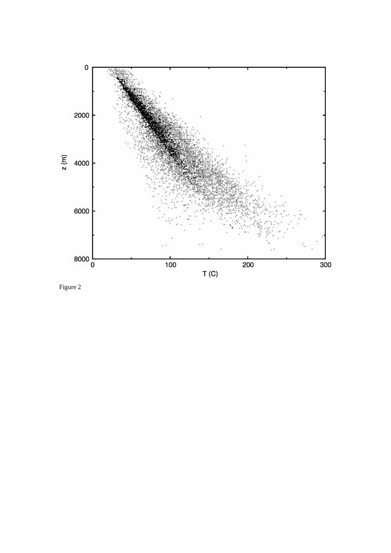
Figure 2

Figure 3

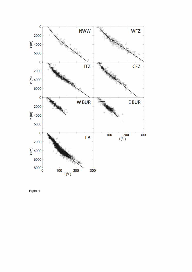
Figure 4

Figure 5

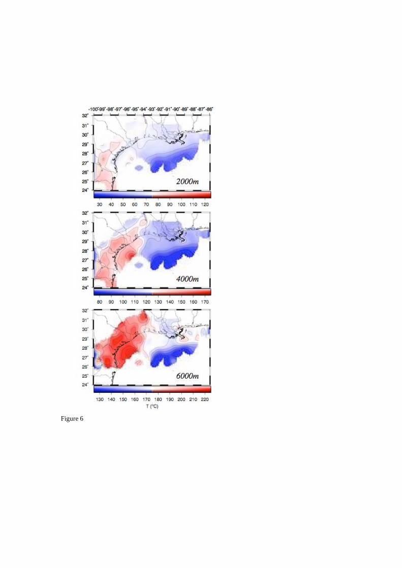
Figure 6

Figure 7

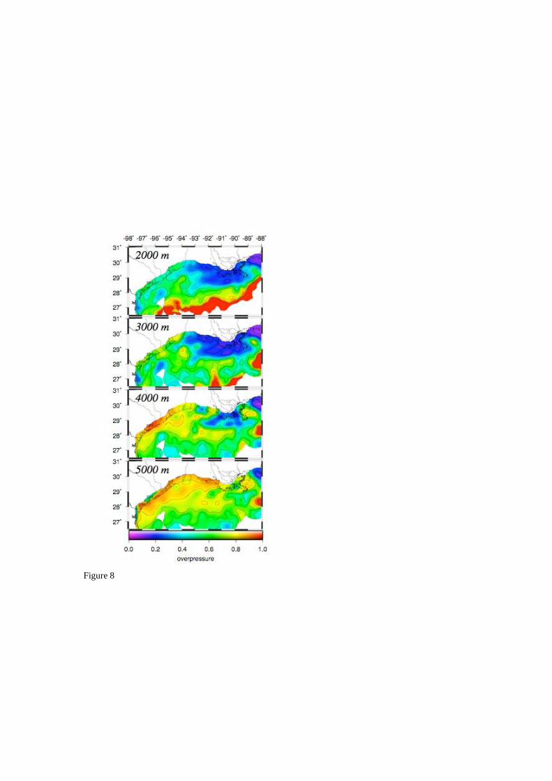
Figure 8

Figure 9

Figure 10

Electronic supplements:

Table E1: Bottom Hole Temperatures. For confidentiality, latitudes and longitudes have been

downgraded to a precision of +/-0.025 degrees (half-size of a lease). zs is ground depth below sea level,

zb is the depth of measurement below sea level, T is the temperature in Celsius.

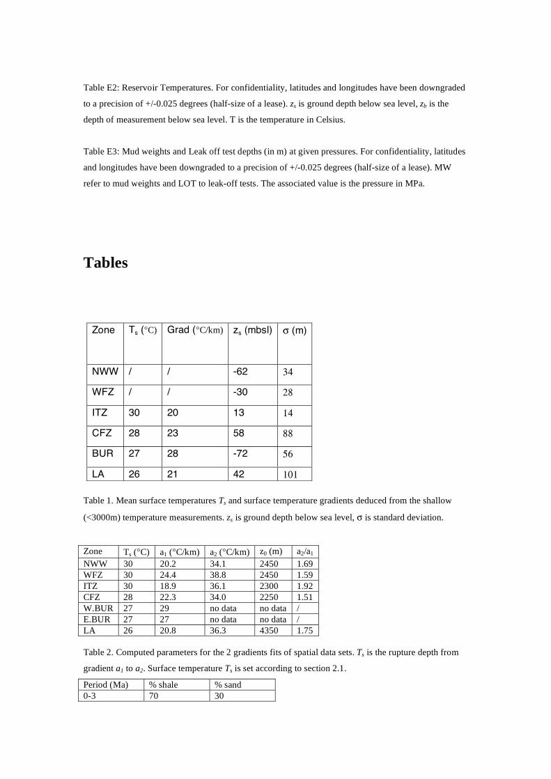
Table E2: Reservoir Temperatures. For confidentiality, latitudes and longitudes have been downgraded

to a precision of +/-0.025 degrees (half-size of a lease). zs is ground depth below sea level, zb is the

depth of measurement below sea level. T is the temperature in Celsius.

Table E3: Mud weights and Leak off test depths (in m) at given pressures. For confidentiality, latitudes

and longitudes have been downgraded to a precision of +/-0.025 degrees (half-size of a lease). MW

refer to mud weights and LOT to leak-off tests. The associated value is the pressure in MPa.

Tables

Table 1. Mean surface temperatures Ts and surface temperature gradients deduced from the shallow

(<3000m) temperature measurements. zs is ground depth below sea level, is standard deviation.

Zone Ts (°C) a1 (°C/km) a2 (°C/km) z0 (m) a2/a1

NWW 30 20.2 34.1 2450 1.69

WFZ 30 24.4 38.8 2450 1.59

ITZ 30 18.9 36.1 2300 1.92

CFZ 28 22.3 34.0 2250 1.51

W.BUR 27 29 no data no data /

E.BUR 27 27 no data no data /

LA 26 20.8 36.3 4350 1.75

Table 2. Computed parameters for the 2 gradients fits of spatial data sets. Ts is the rupture depth from

gradient a1 to a2. Surface temperature Ts is set according to section 2.1.

Period (Ma) % shale % sand

0-3 70 30

Zone Ts (°C) Grad (°C/km) zs (mbsl) (m)

NWW / / -62 34

WFZ / / -30 28

ITZ 30 20 13 14

CFZ 28 23 58 88

BUR 27 28 -72 56

LA 26 21 42 101

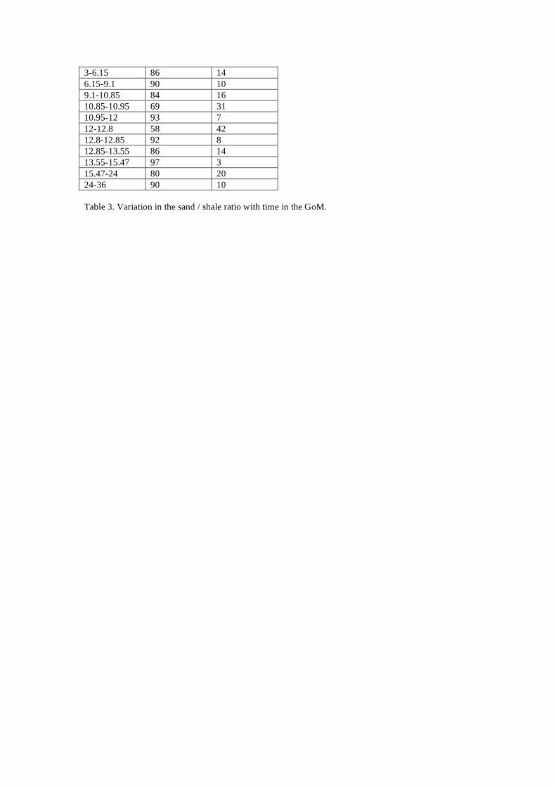
3-6.15 86 14

6.15-9.1 90 10

9.1-10.85 84 16

10.85-10.95 69 31

10.95-12 93 7

12-12.8 58 42

12.8-12.85 92 8

12.85-13.55 86 14

13.55-15.47 97 3

15.47-24 80 20

24-36 90 10

Table 3. Variation in the sand / shale ratio with time in the GoM.