Master Level Thesis

European Solar Engineering School

No.183, December 2013

Thermal Evaluation of a Solarus PV-T collector

Master thesis 18 hp, 2013 Solar Energy Engineering

Student: Jihad Haddi Supervisor: Mats Rönnelid

Dalarna University

Energy and Environmental

Technology

3

Abstract ............................................................................................................................................................. 5

Acknowledgements ...................................................................................................................................... 6

1 Introduction ............................................................................................................................................ 7

1.1 Background ..................................................................................................................................... 7

1.2 Objectives ........................................................................................................................................ 8

1.3 Methods ........................................................................................................................................... 8

2 Theoretical background ..................................................................................................................... 8

2.1 Historic development .................................................................................................................. 7

2.2 Literature study ............................................................................................................................. 8

2.3 Solar irradiation ........................................................................................................................... 11

3 Test of low concentrator T and PV/T collectors ....................................................................... 13

3.1 The PV/T collector ...................................................................................................................... 13

3.2 The T collector ............................................................................................................................. 13

3.3 Test of thermal collectors ........................................................................................................ 14

3.4 Starting up the test rig ............................................................................................................. 17

3.5 Uncertainties in test results .................................................................................................... 18

4 Collector efficiency ............................................................................................................................. 18

4.1 Irradiance ....................................................................................................................................... 19

4.2 Optical losses ............................................................................................................................... 19

4.3 Thermal heat losses from the collector .............................................................................. 20

4.4 Evaluation of thermal performance ..................................................................................... 21

5 Thermal Measurements and Results ............................................................................................ 21

5.1 Measurement set-up ................................................................................................................. 21

5.1.1 Measurements using the test rig ...................................................................................... 21

5.1.2 Measurements of irradiance .......................................................................................... 23

5.1.3 Temperature measurements .......................................................................................... 23

5.1.4 The solar collector test rig .............................................................................................. 23

4

5.2 Measurement results ...................................................................................................................... 24

5.2.1 The effect of one trough on the other ....................................................................... 24

5.2.2 Thermal efficiency of the T collector ........................................................................... 25

5.2.3 Annual energy output ...................................................................................................... 27

6 PVT Collector test ............................................................................................................................... 33

6.1 Influence of the electrical on the thermal power ....................................................... 33

6.2 Thermal efficiency of the PVT collector .......................................................................... 34

6.2.1 Excluding electricity production ................................................................................... 35

6.2.2 Including electricity production .................................................................................... 36

8 Discussion .............................................................................................................................................. 38

9 Conclusion ............................................................................................................................................. 40

10 Suggestions for future works ..................................................................................................... 41

References ..................................................................................................................................................... 42

5

Abstract

Low concentrator PV-T hybrid systems produce both electricity and thermal energy;

this fact increases the overall efficiency of the system and reduces the cost of solar

electricity. These systems use concentrators which are optical devices that concentrate

sunlight on to solar cells and reduce expensive solar cell area. This thesis work deals

with the thermal evaluation of a PV-T collector from Solarus.

Firstly the thermal efficiency of the low concentrator collector was characterized for

the thermal-collector without PV cells on the absorber. Only two types of paint were

on the absorber, one for each trough of the collector. Both paints are black one is

glossy and the other is dull,. The thermal efficiency at no temperature difference

between collector and ambient for these two types of paint was 0.65 and 0.64

respectively; the U-value was 8.4 W/m2°C for the trough with the glossy type of paint

and 8.6 W/m2°C for the trough with dull type of paint. The annual thermal output of

these two paints was calculated for two different geographic locations, Casablanca,

Morocco and Älvkarleby, Sweden.

Secondly the thermal efficiency was defined for the PV-T collector with PV cells on the

absorber. The PV cells cover 85% of the absorber, without any paint on the rest of the

absorber area. We also tested how the electrical power output influences the thermal

power output of the PV-T collector. The thermal and total performances for the PV-T

collector were only characterized with reflector sides, because of the lack of time we

could not characterize them with transparent sides also.

6

Acknowledgements

I would like to thank my supervisor, Dr. Mats Rönneld, for the constructive comments,

warm encouragement and advice. I have been extremely lucky to have a supervisor

who gave me many suggestions to improve my work.

Special Thanks to the Solarus team for giving me an opportunity to work on their

prototype and for being supportive.

I would like to express the deepest appreciation to all members at European Solar

Engineering School, Borlänge, In particular the technicians, Manos Psimopoulos and

Kent Börjesson.

I thank European Solar Engineering School for permission to use the Solar Energy

Research Center, test rig and the roof to make this thesis work.

Finally I would like to say that without the guidance of god and the Love of my

classmates, this thesis would not have been possible.

Thanks to every single person who helped in making this thesis work happen.

7

1 Introduction

1.1 Background

Photovoltaic electricity comes from the conversion of sunlight into electricity in

semiconductor materials such as silicon which is covered with a thin inductive layer.

These photosensitive materials have the property of releasing their electrons under

the influence of external energy. This is the photovoltaic effect. The energy is supplied

by photons (light components) that bombard the material causing the electrons to be

released.

The solar radiation and is able to penetrate the glass to the absorber, reflection losses

from the glass are absorbed, the absorber heats a network of copper pipes trough

which water circulates. This technology which we call a solar collector produces hot

water or heat. All devices that act as solar collectors are increasingly integrated into

the sustainable architecture projects. (Renewable energy. 2013)

The prototype for this work combines two technologies; also the concentration of the

irradiance, this prototype is a low concentrating collector, PV-Thermal (PV-T). This

type of collector has mainly one aim which is to reduce the price of electricity, by

reducing the PV area and compensating by the concentration of the light on this

smaller area. This makes it more cost effective, because we attain the same amount of

electricity produced with lower PV cell area.

This thesis deals with a prototype under this reference CPC, PV-T, 300W, built in

Solarus AB, Älvkarleby, Sweden. Their mission is to make it more attractive for

customers, and more cost effective, by improving the thermal efficiency, also the

electric part and to increase the system’s total energy output.

The work which will be done in this thesis, consist of first determining the thermal

performance, heat losses and optical efficiency, of this prototype which has two

absorbers painted with two different paints, one called Solkote and it is glossy, and

the second is painted with dull paint. Then working on the same collector but with PV

cells on the absorber, and also defining the thermal performance, to see how the PV

affects the thermal performance, and to what extent this co-generation is efficient.

8

1.2 Objectives

The main aims for this project are to:

-Analyze the thermal test equipment (test rig), difficulties with using it and how it will

operate with this kind of collectors.

-Determine the limitations and uncertainties of the data measured.

-Compare the performance of using different receiver paints in Solarus Thermal

collector.

-Compare the thermal performance when the PV cells are operating and when they

are not in Solarus PV-T collector.

1.3 Methods

The basic method to define the performance is to measure the Inlet temperature Tin

and the outlet one Tout, by exposing the collector to the solar radiation, with a known

azimuth and tilt angle. After these tasks are done, the flow rate and the total of

solar radiation on surface of the collector will be measured, thermal output and test

rig will be measured, also a calculation of the yearly performance difference of both

troughs will be found, and eventually an evaluation will be carried out.

2 Theoretical background

2.1 Historic development

For centuries the basics of solar heating have been known and used. In the 4th century

BC the ancient Greeks heated their homes thanks to the passive solar energy, in the

18th century there were some ideas on how to actively convert solar energy to heat.

When determining how the highest temperature could be achieved in a “hot box” by

scientists testing the phenomenon, the box was insulated with glass lid. Black painted

metal tanks were used by people in the 19th century to as solar water heaters; they

would put them on the roofs. However, as soon as the sun goes down the water

inside these tanks cool down and also this technique takes a long time to heat the

water. In 1891 this technique with the “hot box” was combined with the black metal

tanks to give the first commercial solar water heater in the world by Clarence Kemp

from Baltimore, USA. These collectors were of a black metal tanks being put inside

boxes and covered with glass lids, capturing the sunlight. A similar system to the solar

systems used today was developed in 1909 by Bailey in 1909, in this system the tank

and the solar collector are separated to two units, here the tank is insulated with the

9

possibility of placing it inside the house, keeping the water hot for a longer period of

time than the previous one. (Butti & Perlin, 1980)

In later years, the market for solar thermal energy started to increase in the United

States, but then failed as gas and electricity became available at a low price. In the

1950s, 1960s and 1970s greater attention was paid to solar thermal energy in all

countries worldwide. Technology was introduced in Japan, where the market has

grown very rapidly. Also in countries around the Mediterranean Sea, Australia and

Greece, in these areas people started using solar water heaters and the market has

lasted for a long time (ESTIF, 2006). When the oil embargo took place, in 1973, and

the prices of oil increased greatly, the solar water heater industry restarted again in

many places.

In the mid-1980s, the prices of oil became stable then, sales of solar collectors

dropped. (Butti and Perlin, 1980)

During the time between 1981-1989, more than 100 PV-T liquid collectors were

manufactured and installed by SunWatt located in USA, and worked on low-

concentrating PV-T and started development in 1978 (Komp, 1985). During the 80s,

many projects started to appear in Europe (Schwartz, 1983).

2.2 Literature study

Recently a new technology to heat water has emerged, this time it is not a new flat

plate collector but it a concentrator PV-T (photovoltaic/Thermal Hybrid), it has two

functions above the conventional plate. 1) concentrating solar radiation on the

receiver, and 2) cogenerating thermal and electrical output together. To investigate

the thermal performance of concentrating PV-T, many sources were reviewed during

this thesis work. Much work to test and evaluate the thermal performance of this kind

of collector has been done, especially in the area of thermal efficiency. Some of this

research is outlined in this section.

(Zondag et al., 2003) has shown that an uncovered sheet-and-tube collector was

performing poorest at zero reduced temperature because of its large heat losses.

They discovered also that the sheet-and-tube collectors with cover have higher

efficiency. (Zondag et al., 2003) concluded that for the combined PV-T collector, the

total efficiency at zero reduced temperature is over 50%. Therefore it produces a

higher yield per unit area than a thermal collector and PV located next to each other.

The measurements of (Bernardo et al., 2011) have showed that the hybrid electricity

efficiency 0.064 and the optical one is 0.45 while the U-value is 1.9 W/m2°C, they also

10

declared that these values are poor when compared to the parameters of standard PV

modules and flat plate collectors.

To find out how the absorption happened in the absorber surface below the PV. An

experiment done by (Cox and Raghuraman, 1985) shows that there was an increase in

thermal efficiency, from 34% to 39% thanks to a back contact gridding in combination

with a separate absorber below the PV. (Zondag et al., 2003) found out that with the

channel underneath transparent PV with a secondary absorber at the back, the

thermal efficiency was 63% compared to 60% for a PV-T channel collector with the

channel underneath opaque PV.

To increase the heat transfer from PV cells to absorber, a conventional PV-laminate

was connected to a sheet-and-tube absorber thanks to aluminum-oxide-filled two-

component epoxy glue by (De Vries, 1998). It was known that the glue has a heat

conductance of 0.85 W/m2K due to the aluminum oxide, but in reality a lower value

was found, this caused a heat transfer coefficient of 45 W/m2K between the cells and

the absorber. Theoretical calculations showed that this thermal resistance reduced the

annual average efficiency of his collector from 37% to 33%. Other reports of

(Sudhakar and Sharon, 1994) showed that there was a very poor thermal contact

between the PV-laminate and water; they determined that there was 15°C difference

of temperature between them. This poor contact was assigned to the thermal

resistance of the PV-laminate and the fact that tubes are tightened to the absorber.

But in another work of (Hendrie, 1982) the same results were found, the large

difference between the temperature of PV cells and water, here meant the water

temperature was 28°C while the cell temperature was 63°C, the difference in this work

is that this large delta in temperature was ascribed to the fact of having a mechanical

seal which left large air gaps between absorber and the tubes. (Raghuraman, 1981)

Reports on a PV-T liquid system composed of solar cells that are glued directly to the

thermal absorber plate with an insulating layer of electrical insulation to avoid the

contact between them and the absorber plate, which could cause a short circuit.

The PV-laminate consisting of a thick layer of silicone, with a thermal conductivity of

0.2 W/m2°C and a thickness of 0.5 cm, gave a heat transfer of 40 W/m2°C, he found a

temperature difference of 12°C between the absorber and the PV-laminate because of

the high thermal resistance of the silicon layer, therefore the thermal efficiency was

reduced by more than 10%.

Many efforts have been made to improve the heat transfer from the absorber to the

liquid, such as the work of (De Varies, 1998) which proposed of having a dual-flow PV-

11

T collector, with a water inlet above the PV and the water exit below the PV, plus an

additional insulation which was an air layer between the PV-laminate and the water

exit channel, in order to keep the PV cells as cool as possible. The design is shown in

Fig 2.1. After simulating this system, it showed an improvement in the thermal

efficiency thanks to the insulating air layer, the results showed, 66% a thermal

efficiency and 8.5% electrical efficiency, the electrical efficiency is high thanks to the

cold inlet.

Figure 2.1 Two absorbers model of De Vries [43].

The annual yield of PV-T system could be improved by 2% according to De (Varies,

1998), if water channels are used in the bottom of PV cells, instead of a sheet-and-

tube construction. Annual production could be even increased by another 6%, if a

water layer is over the laminate PV-T instead of below it. However, the average

electrical efficiency was reduced from 6.6% to 6.2% due to the extra layer of glass.

2.3 Solar irradiation

Extraterrestrial Solar Spectral Irradiance and the one of a blackbody are similar, at

approximately 5780 K, the spectrum’s emissivity is considered to be equal to 1.

Hydrogen atoms are combined to helium while energy is liberated and radiated as

electromagnetic radiation, radiation is dispersed in all directions from the sun and the

radiation incident on the earth outside of the atmosphere is 1367 W/m2 (Duffi &

Beckman, 2006), also called the solar constant. This is an annual average as the solar

radiation varies slightly over the year (from 1322 in July to 1412 W/m² in December),

because of the earth slightly elliptical orbit around the sun and variations in solar

activity (Duffi & Beckman, 2006). The amount of solar radiation which reaches the

earth is 1000 W/m2, it is reduced due to the influence of many atmospheric gases,

such as; CO2 and water vapor, which absorb and scatter solar radiation of different

wave lengths.

Solar spectrum is the abbreviation of spectral distribution of electromagnetic

radiation coming from the sun, its wavelength extends from 0.3 um to 3.0, including

visible light, ultraviolet and near infrared radiation. The absorptence of solar radiation

12

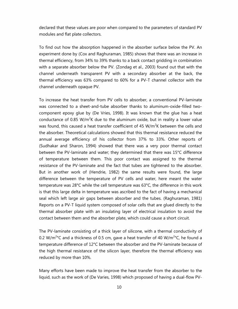
by atmospheric gases and radiation from the sun before and after passing via the

atmosphere is shown on Fig 2.3.

Figure 2.2 The solar spectrum for a black body at 5800 k, an AM0 spectrum

and an AM2 global spectrum, and the absorption bands of

different gases and the absorption bands of different gases. Figure

from Itaca (2013)

Lower irradiance reaches the ground at higher latitudes, because the angle of

incidence of solar irradiance on the earth’s surface is higher. Solar radiation travels

trough longer distance in the atmosphere to reach higher latitude, which makes it los

more energy by absorptence and reflectance before reaching the earth, therefore the

average irradiance at high latitude is lower than lower latitudes. The irradiance is also

reduced due to the humidity and concentration of the particles in the air. The annual

global irradiance on a horizontal surface varies depending on the location from 640 to

2300 kWh/m2.

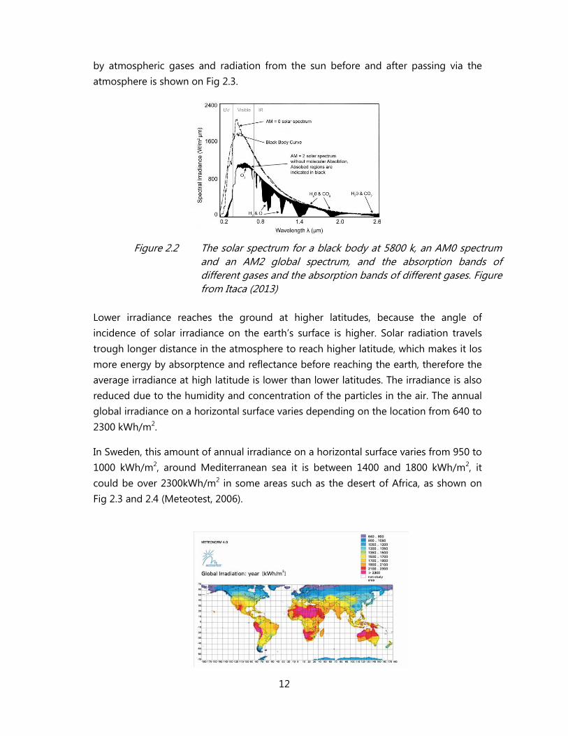
In Sweden, this amount of annual irradiance on a horizontal surface varies from 950 to

1000 kWh/m2, around Mediterranean sea it is between 1400 and 1800 kWh/m2, it

could be over 2300kWh/m2 in some areas such as the desert of Africa, as shown on

Fig 2.3 and 2.4 (Meteotest, 2006).

13

Figure 2.3 the annual global irradiation throughout the world, measured on a

horizontal surface. Figure from Meteotest (2006).

Figure 2.4 the annual global irradiation in Europe, measured

on a horizontal surface. Figure from Meteotest (2006).

3 Test of low concentrator T and PV-T collectors

3.1 The PV-T collector

For the low-concentrating PV-T used in this work is CPC, PV-T, 300W shown in the

Figure 3.1, 304 cells are glued on both sides of the absorber which is water cooled, so

here they are covering about 85% of the absorber, with a maximum Power rating at

STC up to 275 W, Vpmax 18.14V, Ipmax 14.76A, Voc 22.8V and Isc 16.04A. According to

Solarus AB (2013), thermal heat loss coefficient of this type of low-concentrating PV-T

is about 1.9 W/m2°C.

Figure 3.1 PV-T collector from Solarus

14

The solar irradiation received on the concentrator aperture, is focused on the absorber

area which is covered with solar cells, then this solar radiation is partly converted into

electricity, and the rest to thermal energy, generally this thermal energy is hot water

or air. The performance of a PV-T system is dependent on different parameters, such

as the location (climatic conditions), type of solar cell, and the mass flow rate of fluid.

The low-concentrators PV-T have some challenges, such as using a cheap reflector

with high reflectance which can concentrate the sun with a high efficiency, track the

sun, and adequately cool the solar cells to maintain high energy output.

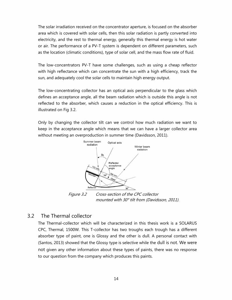
The low-concentrating collector has an optical axis perpendicular to the glass which

defines an acceptance angle, all the beam radiation which is outside this angle is not

reflected to the absorber, which causes a reduction in the optical efficiency. This is

illustrated on Fig 3.2.

Only by changing the collector tilt can we control how much radiation we want to

keep in the acceptance angle which means that we can have a larger collector area

without meeting an overproduction in summer time (Davidsson, 2011).

Figure 3.2 Cross-section of the CPC collector

mounted with 30° tilt from (Davidsson, 2011).

3.2 The Thermal collector

The Thermal-collector which will be characterized in this thesis work is a SOLARUS

CPC, Thermal, 1500W. This T-collector has two troughs each trough has a different

absorber type of paint, one is Glossy and the other is dull. A personal contact with

(Santos, 2013) showed that the Glossy type is selective while the dull is not. We were

not given any other information about these types of paints, there was no response

to our question from the company which produces this paints.

15

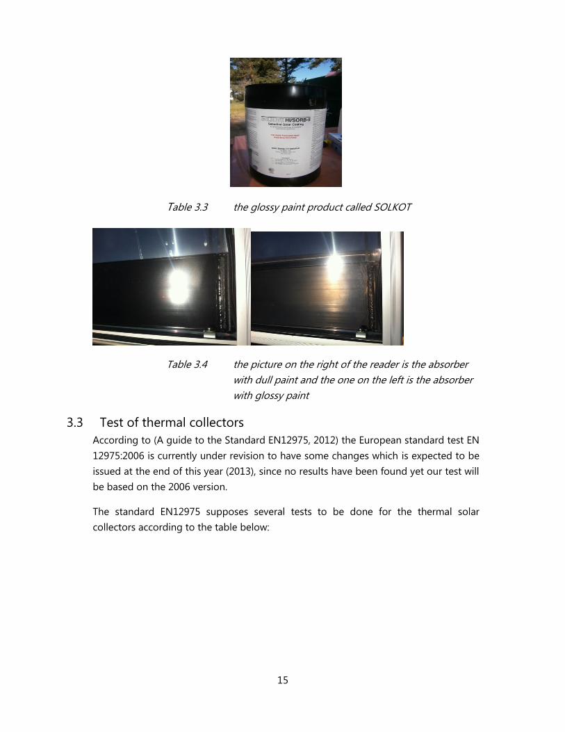
Table 3.3 the glossy paint product called SOLKOT

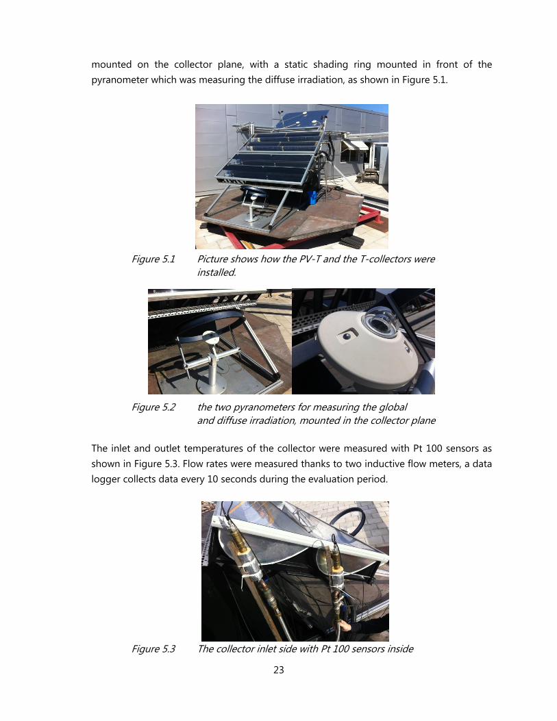
Table 3.4 the picture on the right of the reader is the absorber

with dull paint and the one on the left is the absorber

with glossy paint

3.3 Test of thermal collectors

According to (A guide to the Standard EN12975, 2012) the European standard test EN

12975:2006 is currently under revision to have some changes which is expected to be

issued at the end of this year (2013), since no results have been found yet our test will

be based on the 2006 version.

The standard EN12975 supposes several tests to be done for the thermal solar

collectors according to the table below:

16

Table 3.1 Different tests for the collector adapted from

(A guide to the Standard EN12975, 2012)

In this thesis project we are going to focus on characterizing the thermal performance

of our low-concentrating collector which is based either on the steady state (SS) or

Quasi-Dynamic Testing (QDT).

According to (Pettersson, Kovács and Perers), Steady State (SS) is a simplified test

method originating from Ashrae 93-77 and ISO 9806 standards with the following

parameters Diffuse fraction <20% and irradiance GT > 800 W/m2, while these

parameters in the EN 12975 are Diffuse fraction < 30% and irradiance G > 700 W/m2.

The major drawback of this method is that we can use only the data which was

recorded under very constant conditions when the collector is in “Steady State”. The

collector has also an additional uncertainty due to the use of an incident angle

modifier for the hemispherical which is dependent also on the diffuse fraction

dominating while doing the measurement, these drawbacks make the steady state

test only suitable for collectors with thermal performance, which are not dependent

on the nature of irradiance neither beam nor diffuse, as a result this test method is

not suitable at all for the concentrating collectors. This had been shown in the topic

report by (Fischer et al., 2012).

Quasi-Dynamic Testing (QDT) was presented in the EN 12975-2001, comparing to (SS)

this method has many advantages, such as it gives us the possibility to characterize

different types of collectors, ambient and operating conditions and delivers a

complete characterization of the collector trough compared to the (SS).

Test Test procedure

High

temperature

resistance

1 h with GT > 1000 W/m² and ambient

temperature 20 – 40 °C, wind < 1 m/s

Exposure

according to ISO 9806-2 Class A 30 days with H

> 14 MJ/m² 30 h with G >850 W/m² and

Ta>10°C

Rain

penetration Test duration 4 h

Impact

resistance

according to ISO 9806-2 or with 7.5 g ice ball 10

times with 23 m/s ± 5%

Thermal

performance

Pre-conditioning 5h with G > 700 W/m², diffuse

fraction < 30 %. Steady State or Quasi-Dynamic

Testing.

17

3.4 Starting up the test rig

This part defines almost all the problems we met to make the test rig works.

Before testing the collectors we had to find out how the test rig works and what was

wrong with it, and then we had to replace and fix the components which were not

working correctly.

In Fig 3.5 we can see the pump which drive the hot water to the borehole which was

broken so we had to order it from Denmark. Usually if one of the pumps is broken

then we have a the second solution, this time it was the chiller, however the chiller

wasn’t working, but it was not possible to get it to work properly due to causes

unknown.

Figure 3.5 show the two pumps for the borehole and chiller

In Figure 3.6 the two flow meters displays don’t show the same flow rate for both

collectors, which was the biggest problem before testing the collectors, we tried many

solutions, such as; making a closed loop without passing by the collector, to see if the

collectors are the problem in having this difference in the flow rate, but we found out

that they are not, so we had to keep investigating as to why the flow rate was

different from in both collectors.

18

Figure 3.6 flow meters display for collectors, the PV-T and the thermal

one

We thought maybe the flow meters didn’t work well, so we bought two new flow

meters as shown in Fig 3.7, we tested them separately in series they showed the same

flow rate for both, which means that they have no problem. We tried to connect them

to the test rig, but again two different flow rates were observed in the two flow

meters, after connecting them to the test rig and to collectors. We tried to adjust the

flow rate via the valves but it is very difficult to have the same flow rate for both

collectors in the same time, since we didn’t have this condition we couldn’t start our

testing.

Figure 3.7 The new flow meters with their displays

Finally we found out that the test rig was built to test big collectors which require a

high flow rate so at a high flow rate we only had 1% error but at a low flow rate the

error is big (Persson, 2013),

19

We could just adjust the flow via the valves, but it is difficult to control the flow rate

and make it similar in both collectors for a low one, because the valves were designed

for high flow. So for a low flow which we assumed at 20l/h we need a valve with Kv

value of 0.064 with differential pressure of 0.2 which we divided by 2 because we have

two loops which needs two valves, according to this Equation in (Peres et al., 2012).

3.5 Uncertainties in test results

According to (Pettersson, Kovács and Perers), an accredited test laboratory showed

that the overall value of uncertainty of the solar collector efficiency is 3% to 10% for

the calculated energy gain. This value depends on which test method was used for

designing solar thermal installations.

Many factors have to be taken into account when we look at the uncertainty of the

final results, such as the measurement uncertainty during testing, material property

uncertainties and model uncertainty. The Table 3.2 shows some different uncertainties

which influence the final results.

Table 3.2 Measured uncertainties in collector testing achievable

at a professional test lab adapted from (Pettersson, Kovács

and Perers)

Measured Standard

uncertainty

Aa [m²] 0,1%

G [W/m²] 2%

[kg/s] 0.4%

Tin [°C] +-0.04/1°C

Te [°C] +-0.04/1°C

(Te-Tin) [°C] +-0.02/1°C

Ta [°C] +-0.2/1°C

4 Collector efficiency

The thermal performance of solar collector is defined thanks to its optical properties.

Not all of the incident solar radiation coming from the sun is absorbed by the

absorber; there are some optical losses, such as, reflection of the glass, absorption in

the glass and reflexes between the cover and the absorber. Only what remain from

solar radiation after the optical losses is absorbed by the absorber. From the absorber

the heat is transferred to the liquid through conduction and convection, but not all

the heat is transferred because also the absorber has its own losses, mainly through

20

radiation and convection, also conductive heat losses, insulation of the piping and

collector is important.

Irradiance which is successfully absorbed by the absorber is reduced by the heat

losses. As described by Equation (1).

q = S - UL(Tpm-Ta) Eq. (1)

Tpm Temperature of the absorber

Ta Temperature of the ambient air

UL Heat loss coefficient (insulation capacity of the collector in (W/m²K)

S Absorbed radiation

4.1 Irradiance

The hemispherical solar irradiation GT on a tilted solar collector, is the global solar

irradiation (diffuse and beam) on the collector.

The ratio of the power to the irradiance gives the instantaneous efficiency of a solar

collector. As shown in Equation (2)

η=q/GT Eq. (2)

4.2 Optical losses

The losses of solar radiation which happens due to absorption and reflection in the

cover (glass) and the absorber, these losses are described by the optical efficiency of

the collector. Also optical losses in the reflector must be taking into account in the

case of concentrating collectors.

Optical losses in the glass cover

The irradiation incident on the absorber is reduced, because some of this irradiation is

lost by reflection and absorption in the glass. At normal incidence, a flat clear glass

with 4 mm thickness has a transmittance of approximately 83%. An increase in the

transmittance of glass material has been developed, by reducing iron content and

anti-reflection treatment. The reduced iron content glass has a transmittance of

approximately 90%. The commonly used glass is the antireflection treated glass with a

transmittance up to 95% (Brogren et al., 2000).

Optical losses in reflectors

21

The optical losses are different from reflector to other depending on the material.

Many studies have been done on aluminum and steel, these studies showed that the

steel can last longer than the aluminum, especially when it comes to outdoors, but

higher reflectance for the aluminum of 90% and 65% for steel, but aluminum

reflectors which are anodized have proved to be stable in the long-term (Brogren et

al., 2000).

Absorbed energy from solar radiation

The absorbed energy, S, shown in Equation (3), is the global irradiance in the collector

GT (beam and diffuse) after being reduced by the optical losses. The optical losses are

described thanks to the term ( )n, this term includes also the multiple reflections

between the absorber and the cover.

S = GT ( )n Eq. (3)

The temperature of the absorber is higher than the temperature of the liquid inside

the absorber, this difference in temperature due to heat losses is expressed by the

collector efficiency factor, F’, this factor depends on the temperature, it includes

different heat resistances which happens in the absorber, F’ influences the heat losses

and the energy absorbed. The Equation (1) of the power, q, becomes as in Equation

(4), if the factor F’ is taken into account. In the Equation (4), (Tpm-Ta) is replaced by the

difference between the ambient temperature, Ta, and the mean temperature of the

liquid inside the absorber, Tm. this expression is the most common, since Tm is easy to

measure, by measuring the inlet and outlet of the fluid temperature, and calculating

the average temperature between, Tin and Tout, as in Equation (5). (Perers, 2012).

q = GT F’( )n _ F’UL(Tm-Ta) Eq. (4)

Tm= (Tin-Tout)/2 Eq. (5)

The term F’( )n is the optical efficiency and referred as 0, therefore the power can

be expressed as in Equation 8, for more simplification.

q = 0.GT - F’UL(Tm-Ta) Eq. (6)

4.3 Thermal heat losses from the collector

Thermal heat losses from the solar collector happen through the back, the top and

the edges of the collector, the heat loss coefficient is F’UL, the heat losses from the

22

collector are the difference between the mean temperature of the liquid in the

collector, Tm and the temperature of the surroundings multiplied by the heat loss

coefficient, as F’UL(Tm-Ta).

4.4 Evaluation of thermal performance

Measurements of the temperature inlet and outlet of the liquid in the collector, the

ambient temperature, hemispherical radiation in the collector plane and the flow rate,

allow us to evaluate the thermal performance of solar collectors, according to the

European Standard (EN 12975). The overall efficiency is defined as in Equation (7),

with Cp is the specific heat capacity; Ac is the aperture area of the collector and is

the mass flow rate. The specific heat capacity of the water varies with water

temperature; therefore it should take into an account the mean temperature of the

liquid in the collector.

= Cp . m . (Tout-Tin)/GTAC Eq. (7)

The thermal performance measurements make the calculation of the optical efficiency

0 of the solar collector possible, by rearranging the Equation (6) in Equation (8).

0 = q . F’. UL . (Tm-Ta)/GT Eq. (8)

5 Thermal Measurements and Results

5.1 Measurement set-up

This part describes the measurement set ups, techniques and equipment used for these

measurements. They were mainly done outdoors in the field trials at the Solar Energy

Research Centre (SERC).

5.1.1 Measurements using the test rig

The evaluation of the concentrating collectors has been done from outdoor measurements

using a test rig. The thermal measurements were done between the 6th and the 8th of May

2013 for the thermal collector, and between the 23rd and 30th of May for the PV-T

collector, both measurements took place in the field trials at Dalarna University, Borlänge,

Sweden.

The collectors were facing the south during the measurements with a fixed tilt of 45°.

Global and diffuse irradiation were measured thanks to the two pyranometers, they were

23

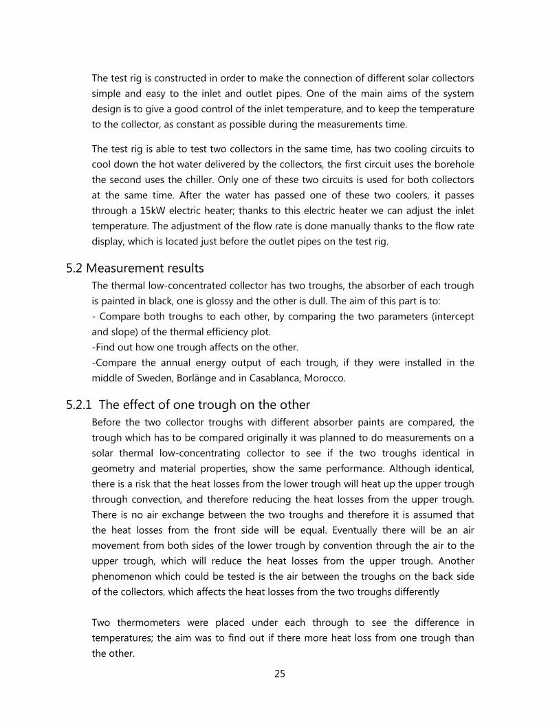
mounted on the collector plane, with a static shading ring mounted in front of the

pyranometer which was measuring the diffuse irradiation, as shown in Figure 5.1.

Figure 5.1 Picture shows how the PV-T and the T-collectors were

installed.

Figure 5.2 the two pyranometers for measuring the global

and diffuse irradiation, mounted in the collector plane

The inlet and outlet temperatures of the collector were measured with Pt 100 sensors as

shown in Figure 5.3. Flow rates were measured thanks to two inductive flow meters, a data

logger collects data every 10 seconds during the evaluation period.

Figure 5.3 The collector inlet side with Pt 100 sensors inside

24

5.1.2 Measurements of irradiance

The measurements of the hemispherical and diffuse solar irradiance have been done

with two pyranometers, with a shading ring for the pyranometer which measures

diffuse irradiance. The beam irradiance is the difference between the hemispherical

and diffuse; it was calculated from this data. The pyranometers were calibrated and

placed in the collector plane.

5.1.3 Temperature measurements

If we want to remove disturbances from the collector thermal capacitance to

the efficiency and measured thermal output, the inlet temperature to the solar

collector must be constant. This is very important since our collector requires a

low flow rate. Pt 100 sensors, a thermopile and temperature sensor of

microchip type (LM35) have been used to measure the temperature during

different measurements, in our case the temperature measurements were

done thanks to Pt 100, for the inlet, outlet and the ambient temperature, (Tout-

Tin) was calculated based on the measurements of Tout and Tin.

5.1.4 The solar collector test rig

The test rig was built to test the thermal performance of different solar thermal

collectors, such as, CPC, vacuum tubes, etc...

The test rig facilitates our stationary collector testing with good repeatability of

the measurements.

Figure 5.4 The solar collector test rig.

25

The test rig is constructed in order to make the connection of different solar collectors

simple and easy to the inlet and outlet pipes. One of the main aims of the system

design is to give a good control of the inlet temperature, and to keep the temperature

to the collector, as constant as possible during the measurements time.

The test rig is able to test two collectors in the same time, has two cooling circuits to

cool down the hot water delivered by the collectors, the first circuit uses the borehole

the second uses the chiller. Only one of these two circuits is used for both collectors

at the same time. After the water has passed one of these two coolers, it passes

through a 15kW electric heater; thanks to this electric heater we can adjust the inlet

temperature. The adjustment of the flow rate is done manually thanks to the flow rate

display, which is located just before the outlet pipes on the test rig.

5.2 Measurement results

The thermal low-concentrated collector has two troughs, the absorber of each trough

is painted in black, one is glossy and the other is dull. The aim of this part is to:

- Compare both troughs to each other, by comparing the two parameters (intercept

and slope) of the thermal efficiency plot.

-Find out how one trough affects on the other.

-Compare the annual energy output of each trough, if they were installed in the

middle of Sweden, Borlänge and in Casablanca, Morocco.

5.2.1 The effect of one trough on the other

Before the two collector troughs with different absorber paints are compared, the

trough which has to be compared originally it was planned to do measurements on a

solar thermal low-concentrating collector to see if the two troughs identical in

geometry and material properties, show the same performance. Although identical,

there is a risk that the heat losses from the lower trough will heat up the upper trough

through convection, and therefore reducing the heat losses from the upper trough.

There is no air exchange between the two troughs and therefore it is assumed that

the heat losses from the front side will be equal. Eventually there will be an air

movement from both sides of the lower trough by convention through the air to the

upper trough, which will reduce the heat losses from the upper trough. Another

phenomenon which could be tested is the air between the troughs on the back side

of the collectors, which affects the heat losses from the two troughs differently

Two thermometers were placed under each through to see the difference in

temperatures; the aim was to find out if there more heat loss from one trough than

the other.

26

Figure 5.5

We measured the two temperatures under both troughs, we found the same

temperature, therefore it can be assumed that any heat losses difference between the

troughs mainly depends on the different absorber paints.

5.2.2 Thermal efficiency of the T collector

This evaluation has been done to show the difference in performance between two

troughs, which belong to the same solar collector. The solar collector was mounted

facing south. The first is painted with dull type of paint which is not selective and the

second is painted with a paint called Solkote and it is glossy which is selective, this

evaluation will show which paint performs better, Therefore we had to vary the flow

rate for different values, from 20 to 90l/h with a step of 10, in order to have different

(Tm-Ta)/GT with different efficiencies, for both troughs and plot the efficiency curve, as

shown on the Figure 4.5, in order to define the optical efficiency and the heat losses.

The inlet and outlet water temperatures were measured using Pt 100, at an average

hemispherical irradiance of 935 W/m2 with varied water inlet temperature from 37°C

to 25°C, which decreased with increasing the flow rate, the ambient temperature was

almost constant at 16°C, with a variation of 1°C during the test and the hot water

reached to a maximum temperature of 53°C. The standard efficiency curves of the two

troughs and results are shown in Figure 5.6 and in Table 5.1.

27

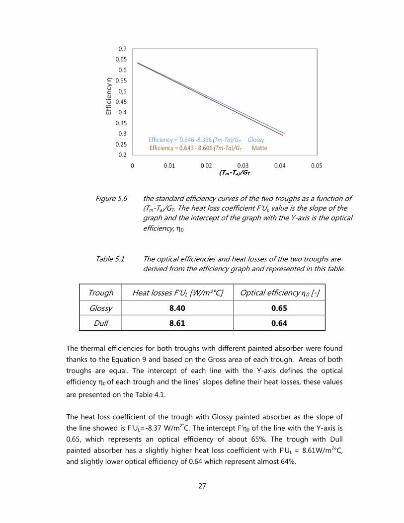
Figure 5.6 the standard efficiency curves of the two troughs as a function of

(Tm-Ta)/GT. The heat loss coefficient F’UL value is the slope of the

graph and the intercept of the graph with the Y-axis is the optical

efficiency, 0

Table 5.1 The optical efficiencies and heat losses of the two troughs are

derived from the efficiency graph and represented in this table.

Trough Heat losses F’UL [W/m²°C] Optical efficiency η0 [-]

Glossy 8.40 0.65

Dull 8.61 0.64

The thermal efficiencies for both troughs with different painted absorber were found

thanks to the Equation 9 and based on the Gross area of each trough. Areas of both

troughs are equal. The intercept of each line with the Y-axis defines the optical

efficiency 0 of each trough and the lines’ slopes define their heat losses, these values

are presented on the Table 4.1.

The heat loss coefficient of the trough with Glossy painted absorber as the slope of

the line showed is F’UL=-8.37 W/m2°C. The intercept F’η0 of the line with the Y-axis is

0.65, which represents an optical efficiency of about 65%. The trough with Dull

painted absorber has a slightly higher heat loss coefficient with F’UL = 8.61W/m2°C,

and slightly lower optical efficiency of 0.64 which represent almost 64%.

28

The two values of heat loss coefficient for the two troughs are quite high, if we

compare them to the value which Solarus company reports on their technical

specification for this collector, because according to (Solarus AB, 2013) this collector

has a heat loss coefficient of only 1.9 W/m2°C, when it works as a PV-T collector with

PV cells as an absorber coating, while the value which was found after the

measurements is about 4 times higher. The high amount of heat loss coefficient will

be discussed later in the discussion.

There are some clear differences between the parameters, of both troughs, According

to (Perers, 2012) only the operating conditions would determine which one should be

used, and the range of values of (Tm-Ta)/GT that we are expecting in an application, to

heat a pool for example, no need for a high difference in temperature between the

ambient and the absorber, in the other extreme case, for example when we make

steam to turn a turbine we need a significant difference in the temperature at high

efficiency for large values of (Tm-Ta)/GT.

The two troughs have to be evaluated on their performance per year, to be able to

compare them and find out which one is the best, in term of annual energy output,

that’s what will be presented in the coming part.

5.2.3 Annual energy output

Annual heat production in Älvkarleby Sweden

According to (Oscar. 2004), the efficiency describes the ratio between the useful and

the supplied energy in a system, for example in solar collectors, this ratio is the heat

produced relative to the incident solar radiation.

The efficiency of a solar collector is dependent upon many factors, depending on the

choice of materials and the operating conditions. When comparing two collectors it is

not enough to just compare the efficiency at one absorber temperature and therefore

we will compare the expected annual output.

To define the output of a solar collector is a complex process. Therefore, Björn

Karlsson has developed a method for simplifying the theoretical determination of the

energy exchange from a solar collector. "Karlsson formula" can be used to calculate

energy exchange with equal conditions for market solar collectors at various

temperatures.

29

The formula of Karlsson which easily calculates the useful energy per unit area is:

QU= GT.F’( )n – F’UL.(Tm – Ta).t (kWh/m2/year) Eq. (9)

QU Annual heat production

t Number of hours when GT>200W/m2

Tm Mean fluid temperature inside the collector

Approximate annual production will be defined, for both troughs to be able to

compare them. In order to start calculating, we need the optical efficiency and the

heat loss factor, which we already have thanks to my measurements done before. If

we assume that the heat transfer factor F’ is equal to one, this means that the mean

temperature of the fluid inside the absorber is equal to the absorber temperature.

(Perers, 2012)

According to (Rönnelid, 2013) a standard solar collector starts delivering some heat,

when the irradiance is approximately above 200 W/m2, to calculate the annual output

of this collector and to have a clear view of its annual output for both troughs, we

must calculate it under two climates. One is a cold climate as Älvkarleby and the

other will be Casablanca, Morocco.

The annual solar radiation for the central Sweden is 800 kWh/m2/year, for the south of

Sweden this value is 1000kWh/m2/year, here we choose to look at central Sweden

where values for Älvkarleby are given as the total of annual hours of sunshine when

GT>200 W/m2, with an average sunshine total hours of 1270 and an ambient

temperature during operation of 13°C. (Oscar, 2004)

30

Table 5.2 this table shows the annual energy output of our collector. The

collector is facing the south; 45°C is the tilt angle. The annual energy

output was calculated for 3 different mean fluid temperature s for the

location of central Sweden, Älvkarleby.

Trough type

Global

annual

radiation

on a

tilted

surface

[kWh/m2]

Number of

hours when

GT>200W/m2,

[h]

Ta [°C]

Annual heat

production

(kWh/m2) for

different mean

fluid temperature

30°C 40°C 50°C

Trough with Glossy

painted absorber,

F’(τα)n= 0.646 and

F'UL=8.366

800 1270 13 336 230 124

Trough with Mattee

painted absorber,

F’(τα)n= 0.643 and

F'UL=8.606

800 1270 13 329 219 110

If we compare different output from one trough at different mean temperature of the

fluid, we find out that for 30°C, 40°C and 50°C respectively we have 336, 230 and

124kWh/m2/year, so for higher mean fluid temperature we have lower heat output,

because of the increase in the heat losses, as the Equation (9) shows.

Now if we compare the difference in the output of the two types of paint. We have

the three mean fluid temperatures, for 30°C, 40°C and 50°C respectively 3%, 5% and

10% higher yearly heat output for the Glossy (Solkote) paint.

To confirm our results and make them more credible we will calculate the difference

in yearly energy output for both troughs, in a hot climate, therefore we choose

Casablanca, Morocco.

Annual heat production in Casablanca, Morocco

Casablanca (latitude 33 ° 36'N) is Mediterranean climate affected by the cold currents

of the Atlantic sea. The temperature fluctuations are low, with an annual average

maximum daily of 21.2°C and minimum of 13.6 °C.

31

To calculate the annual energy output in Casablanca, as we did for Älvkarleby, we are

going to use Karlsson formula. It was hard to find data for Casablanca contrary to

Älvkarleby; data was taken from (Oscar, 2004). Therefore we had to use software

called Meteonorm.

Meteonorm

Meteotest has performed extensive research activities in cooperation with universities

and the industry. Meteonorm is a product by Meteotest which resulted from research

activities that started in the early 80s.

Meteonorm is a comprehensive meteorological reference, incorporating a catalogue

of meteorological data and calculation procedures for solar applications and system

design at any desired location in the world. It is based on over 25 years of experience

in the development of meteorological databases for energy applications.

Data for Casablanca using Meteonorm

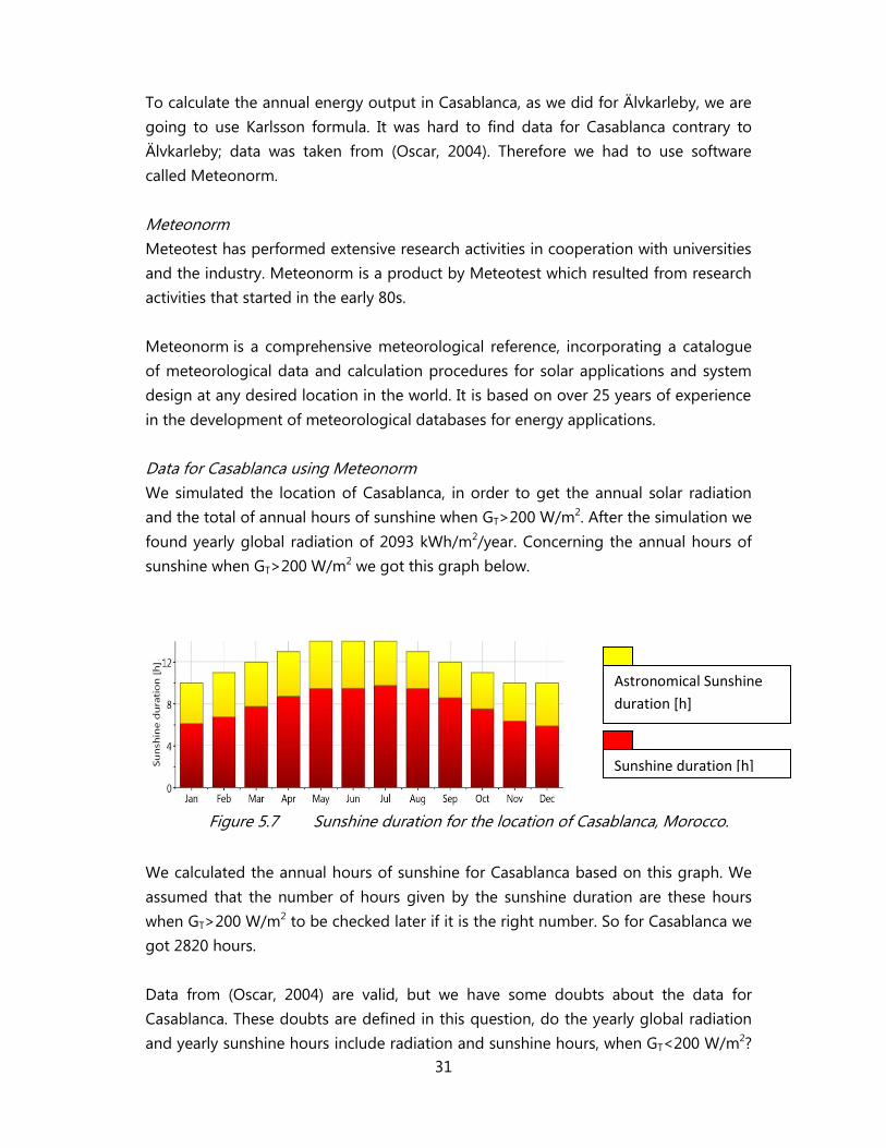
We simulated the location of Casablanca, in order to get the annual solar radiation

and the total of annual hours of sunshine when GT>200 W/m2. After the simulation we

found yearly global radiation of 2093 kWh/m2/year. Concerning the annual hours of

sunshine when GT>200 W/m2 we got this graph below.

Figure 5.7 Sunshine duration for the location of Casablanca, Morocco.

We calculated the annual hours of sunshine for Casablanca based on this graph. We

assumed that the number of hours given by the sunshine duration are these hours

when GT>200 W/m2 to be checked later if it is the right number. So for Casablanca we

got 2820 hours.

Data from (Oscar, 2004) are valid, but we have some doubts about the data for

Casablanca. These doubts are defined in this question, do the yearly global radiation

and yearly sunshine hours include radiation and sunshine hours, when GT<200 W/m2?

Sunshine duration [h]

Astronomical Sunshine

duration [h]

32

An answer for our question will be as a simulation of Älvkarleby city. If we get the

same data as the one given by (Oscar, 2004), it means that the data of Casablanca is

correct.

Data for Älvkarleby city is not available on Meteonorm; therefore we decided to take

the data of the nearest place. Borlänge is the nearest city to Älvkarleby, city, with

available data.

Data of Borlänge using Meteonorm

Borlänge is a city at a latitude of 60.433 [°N] and longitude of 15.5 [°E]. After

simulation of this city we got 1180 kWh/m2 for the yearly global radiation on the tilted

angle. If we compare this value (1180 kWh/m2) of the yearly radiation found on

Meteonorm, to the one from (Oscar, 2004) of 800kWh/m2, which doesn’t include the

radiation when GT<200 W/m2. We found out that they are different. If we assume that

for both locations we have the same yearly radiation on tilted angle, even when they

are slightly different. then the yearly radiation from Meteonorm include the radiation

when GT<200 W/m2. This amount of radiation represents 32% “[(1180-800)/1180]”, So

for Casablanca, the yearly radiation on tilted angle, instead of 2093 kWh/m2 it

becomes 1400 kWh/m2, after taking off the 32% of radiation when GT<200 W/m2.

We want to answer our second question about the yearly sunshine hours when

GT<200 W/m2. As we did before we will calculate it for Borlänge, then compare it to

the one for Älvkarleby, if it is almost the same, we will conclude that the yearly

sunshine hours of Casablanca are correct, if not we will use the rule of thumb.

Figure 5.7 Sunshine duration for the location of Borlänge, Sweden.

From the graph, we found an average of yearly sunshine hours of 1680 hours. If we

compare the number of hours found on Meteonorm for Borlänge, to the one from

(Oscar, 2004) for Älvkarleby. We find out that the hours found on Meteonorm are 25%

higher. Our explanation for this difference, is that the hours of sunshine given by

Meteonorm includes the hours when GT<200 W/m2. As an answer for our question,

Sunshine duration [h]

Astronomical Sunshine

duration [h]

33

we should take off 25% off from the hours which were found for Casablanca, so

instead of 2820 hours we must use 2115 hours to calculate the yearly energy output.

We should mention that the ambient temperature given by Meteonorm is including

the temperature during nights and the time when GT<200 W/m2. We want the

ambient temperature of only the time when heat is produced. Therefore due to some

approximation between the ambient from Meteonorm and the temperature ambient

of Älvkarleby, according to a personal contact with (lakrade, 2013), professor at the

university of Hassan 2, the temperature ambient in Casablanca is about 25°C.

Table 5.3 this table shows the annual energy output of our collector. The

collector is facing the south; 30°C is the tilt angle. The annual energy

output was calculated for 3 different mean fluid temperature s for the

location of Casablanca, Morocco.

.

Trough type

Global

annual

radiation

on a tilted

surface

[kWh/m2]

Number of

hours when

GT>200W/m2,

[h]

Ta [°C]

Annual heat

production

(kWh/m2) for

different mean fluid

temperature

30°C 40°C 50°C

Trough with Glossy

painted absorber,

F’(τα)n= 0.646 and

F'UL=8.366

1400 2115 25 816 638 461

Trough with Mattee

painted absorber,

F’(τα)n= 0.643 and

F'UL=8.606

1400 2115 25 809 627 444

We decided to see how this collector would perform in a hot climate, since we tried it

before in a cold climate, in order to see if there will be any difference in the

performance for both type of paints. As we made for the location of Älvkarleby, the

annual heat production in Casablanca was calculated for three mean fluid

temperatures, 30°C, 40°C and 50°C.

Now that they are simulated to be installed in Casablanca, only a 1% difference exists

between the two types of paint, for the three means fluid temperatures.

34

6 PV-T Collector test

The measurements set-up for the PV-T collector was the same as for the thermal only

collector. Different tests for the PV-T collector were done on the 12th of June, such as

the influence of the thermal and electrical power on each other; a thermal efficiency

curve will be made as we did before for the T-collector

6.1 Influence of the electrical on the thermal power

This test was done to see how the thermal power is affected by the production of

electricity. This took one hour; this hour was divided into three intervals, in order to

see the influence in producing electricity on the thermal power, only thermal

production was allowed in the first and last interval, while electricity production was

allowed in the second interval. Each was 20 minutes long.

Figure 6.1 the graph shows the influence of the electrical power on the

thermal power.

The x-axis represents time and y-axis represents the power. We should mention that

the test lasted one hour which started at 10:30; therefore the thermal power was

increasing with time, due to the position of the sun which was changing with time.

Concerning the x-axis, it starts from zero to 60min. After 20 min the thermal power

had reached 458 W. Then we started producing electricity for 20min. As a result a

decrease in thermal production of about 10% was noticed, but before the 20 min of

electricity production was over, a very big decrease in both electrical and thermal

production happened. This phenomenon was observed for 11min between 37 and 48;

we assume that some clouds were passing in front of the sun during this period,

which caused the decrease in thermal power from 458 to 185 W.

35

After that the period of electricity production and the clouds were gone, we could see

that the thermal power values reset to higher values as observed, before any

electricity production.

6.2 Thermal efficiency of the PV-T collector

6.2.1 Excluding electricity production

Variation in the temperature output of the fluid

To make the thermal efficiency curve for the PV-T collector with and without

electricity production and to be sure that we got to the steady state. A curve was

made; it shows the variation in the fluid temperature output to the time with the

variation of the flow rate. We made this curve to find out when the fluid temperature

output becomes constant. Then we could calculate the efficiency.

Figure 6.2 the graph shows the variation in the temperature output of the

fluid with varying the flow rate.

We expected that the temperature output of the fluid would become constant at a

certain time for each flow rate. Since the temperature input is constant, as a result the

temperature output must be constant at a certain time.

As was previously stated in the measurement set up, the experience took place

outdoors, which means that the sun was our source of energy. Our experience took

one hour and a half, a half hour for each flow rate, in order to get a constant

temperature output, but it was not the case our temperatures output did not really

become constant. An answer about why the temperature output did not stabilize is

that, the PV-T collector was faced south; our experiment started at 11h35, more we

approached to noon the greater the intensity of the sun becomes. For the last 30 min

we changed the flow rate to 90 l/h in order to get lower temperature output, we were

surprised that the temperatures output at a flow rate of 90 l/h was higher than for 50

l/h, even though we had the same temperature input of the fluid for both flow rates.

36

This unexpected result made us have to repeat the measurements with tracking the

collector, but the lack of time prevented this from being done.

Thermal efficiency curve of the PV-T collector

During 30 min for each flow rate, 15, 50 and 90l/h, data was taken every 10sec. to plot

the efficiency curve as we did with the thermal collector. We calculated the efficiency

thanks to the Equation (7), the efficiency was calculated for each 10sec, to plot these

values to (Tm-Ta)/GT. Before we plotted these values we determined an average of the

efficiencies for each flow rate.

Table 6.1 the table contains different efficiencies at zero reduced

temperature with different flow rates for the PV-T without

producing electricity.

mass flow

(l/h) efficiency (Tm-Ta)/GT

15 0.33 0.02

50 0.37 0.02

90 0.39 0.02

As we can see from the table the value of (Tm-Ta)/GT for the flow rate of 90 l/h is

higher than the one for 50 l/h. this difference is due to the temperature of the fluid

outlet which higher when a flow rate of 90 l/h is used.

Based on this data we plotted these efficiencies to different (Tm-Ta)/GT and we got the

following curve.

Figure 6.3 the efficiency curve of the PV-T trough without producing

electricity

37

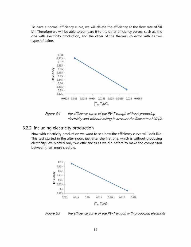
To have a normal efficiency curve, we will delete the efficiency at the flow rate of 90

l/h. Therefore we will be able to compare it to the other efficiency curves, such as, the

one with electricity production, and the other of the thermal collector with its two

types of paints.

Figure 6.4 the efficiency curve of the PV-T trough without producing

electricity and without taking in account the flow rate of 90 l/h.

6.2.2 Including electricity production

Now with electricity production we want to see how the efficiency curve will look like.

This test started in the after noon, just after the first one, which is without producing

electricity. We plotted only two efficiencies as we did before to make the comparison

between them more credible.

Figure 6.5 the efficiency curve of the PV-T trough with producing electricity

38

7 Global results

Figure 7.1 the efficiency curve s of the PV-T and thermal collector, with two

types of paint and for the PV-T with and without electricity

production

The trough with PV-laminate layer has a very important heat loss value when it

produces electricity in parallel to heat, comparing to the same one without producing

electricity. This important amount of heat losses could be justified by the fact of

producing electricity. In addition the heat losses which we loose by conduction,

convection and radiation, we have losses due to the production of electricity. A very

strange result was found, the through with the PV-laminate has greater efficiency at

zero reduced temperature while producing electricity than without. It should be the

contrary.

For the case of the two troughs with two different paints, both of them dull and glossy

type of paint, they perform at almost the same level at zero reduced temperature

8 Discussion

The results from thermal evaluations of related collectors are compared with the

results for the Solarus CPC PV-T versions in table 8.1. The values were taken with

respect to the active glazed area of the collectors. A similar roof-integrated MaReCo

thermal collector (no PV) with a high efficiency SunStrip absorber and anodized

39

aluminum reflectors (reflectance of 85%) has been included by way of comparison.

(Adsten et al., 2005) It is normal for PV-T collectors to have lower thermal efficiencies

than pure thermal collectors, and is due to the fact that in PV-T, a fraction of the

harvested energy becomes electricity instead of heat.

Table 8.1 Thermal efficiency of comparison Solarus and other collectors.

Absorber with Thermal efficiency [%] Heat losses [W/m2K]

Glossy paint 65 8.4

Dull paint 64 8.6

PV-laminate Layer with EP 74 15.6

PV-laminate Layer without EP 47 6.3

MaReCo Thermal Collector 69 2.4

Absolicon PV-T 56 2.3

The amount of heat losses from the thermal collector is very high compared to the

value which was declared by Solarus AB (2013). Either for the trough with glossy paint

or with Dull, the heat losses were almost 5 times higher than the value announced by

Solarus which is 1.9 W/m2°C. We wonder why we have this large difference between

the origin value of heat losses and the one we found, an explanation for this

phenomenon is that Solarus assumed that they have only 1.9 W/ m2°C of heat loss

coefficient. (Santos, 2013)

The heat losses from the PV-T collector are 3 times higher, this height is explained by

the fact of having only 85% of the receiver area covered by PV cells while the

remaining 15% of has no black paint. If we compare Solarus PV-T to some other

similar collectors as shown in the table 8.1, in terms of 0 (optical efficiency), the

Solarus CPC PV-T performs only slightly worse than the Absolicon PV-T collector; The

PV-T from Solarus has lower efficiencies than a pure thermal collector (the MaReCo).

However, the Solarus PV-T receiver has a very high U-value, which will reduce its

performance in normal working conditions significantly. The Absolicon absorber also

has PV cells, and the metal portion of the absorber is covered with a selective coating,

which may explain its F’UL value being comparable to a MaReCo with a SunStrip

absorber.

The value of heat losses for the PV-T without producing electricity was about 6.5

W/m2°C while the value of heat losses of the PV-T with producing electricity was even

higher with a value of about 15 W/m2°C. This result is not logical; and does not agree

40

with (M. Adsten et al., 2005), they showed that, we should have higher heat losses for

the PV-T with electricity production than without. We think that an error occurred

while doing the measurements for PV-T and gave this strange result. Especially while

doing the measurements with electricity production, they must be repeated however

due lack of time we did not have the chance to do this. Due to the questionable

nature of the data used in making the efficiency curve of PV-T with electricity

production, it is more fitting to compare only PV-T without electricity production with

similar collectors from competitors.

The heat losses and the optical efficiency (graph 4.5) of the two types of receiver paint

are slightly close. We calculated the annual heat production in a cold climate for both

troughs, with two types of paint, Glossy and Dull. We know that the Glossy is selective

but not the Dull (Santos, 2013). The annual heat production was slightly higher for the

glossy type. The difference in the annual heat production was 3%, 5% and 10%

respectively for three mean fluid temperatures 30°C, 40°C and 50°C. According to

(Pettersson, Kovács and Perers), an accredited test laboratory showed that the overall

value of uncertainty of the solar collector efficiency is 3% to 10% for the calculated

energy gain. We calculated again the annual heat production of these two types of

paint in Morocco which is considered as a hot climate. We found for Morocco that

only 1% difference is observed between the two troughs for 30°C, 40°C and 50°C

mean fluid temperature. Because of the short time which this test took, it took only

one day to make this test; we think that this is not enough to make a final judgment

concerning these two kinds of paint.

The electricity production of our PV-T collector represents 10% of the thermal

production according to the test we made when we looked at the power output of

both thermal and electrical.

In this thesis work we did not calculate the electrical efficiency. (Zondag et al., 2003)

concluded in their research that for a combined Photovoltaic-thermal collector the

total efficiency at zero reduced temperature is over 50%, which is the case for us. Only

the thermal efficiency of our PV-T collector with electricity production was about 74%.

This value is too high to be true if we compare it to the other similar collectors. The

data for PV-T with electricity production needs to be checked, the other

measurements for the other types of collectors need to be done for a longer time

than one day.

The efficiency at no temperature difference between collector and ambient for our

PV-T with electricity production was larger than without electricity production, the PV-

41

T trough with electricity production had higher heat losses than without electricity

production, but it had higher efficiency at zero reduced temperature. The results we

found do not agree with what (Zondag et al., 2003) found, when the efficiency at zero

reduced temperature of the sheet-and-tube collector, with and without cover were

compared to each other. (Zondag et al., 2003) found that the uncovered sheet-and-

tube has lower efficiency because of the high amount of heat losses. In our case the

uncovered sheet-and-tube is the PV-T with electricity production, it has to have

higher heat losses than the PV-T without producing electricity.

9 Conclusion

Four thermal efficiencies at no temperature difference between collector and ambient

were defined. Firstly for two thermal troughs with two types of paint, secondly for PV-

T trough while producing electricity and while it is producing only heat. Some of these

results are logical compared to other results found in earlier studies. Other results we

found in this thesis work must be revised and repeated again under controlled

conditions. The annual heat output was calculated in two locations (hot and cold

climate) for the two types of paint, we found that they were slightly different. We can

not judge these two types of paints based on these results, we took only one day for

this measurement, the luck of sunny days and time did not help in giving results with

greater certainty. The U-value which was found for both collectors with all kind of

troughs were extremely high for a commercial product such as this from Solarus. The

U-value from the PV-T while producing electricity was even higher two times than the

other which were found, We explained this value with the fact that we are producing

electricity, measurements for this trough must be done again also.

10 Suggestions for future works

The measurements for both the PV-T and the thermal collectors have to be done

again with longer time. If the measurements will take place in Sweden we suggest

conducting indoor measurements, and then comparing them to the outdoor ones.

The way the absorbers were painted has to be checked.

42

References

H. Davidsson, L. R. Bernardo, and B. Karlsson, "Performance Evaluation of a High Solar

Fraction CPC-Collector System" Journal of Environment and Engineering, 2011, vol. 6,

pages 680-692.

L. R. Bernardo, B. Perers, H. Håkansson and B. Karlsson, "Performance Evaluation of

Low Concentrating Photovoltaic/Thermal Systems: A Case Study from Sweden" Solar

Energy, 2011, Vol. 85, pages 1499-1510.

L. R. Bernardo, H. Davidsson, N. Gentile, J. Gomes, C. Gruffman, L. Chea, C. Mumba, B.

Karlsson, "Measurements of the Electrical Incidence Angle Modifiers of an

Asymmetrical Photovoltaic/Thermal Compound Parabolic Concentrating-Collector"

Engineering, 2013, pages 5, pages 37-43.

B.Perers, C. Bales, T. Persson, H. Zinko, F. Fielder, “ESES Solar Heating Systems and

Storage” Compedium Högskolan Dalarna, 2012.

CEN, European committee for standardization. (2006) “EN 12975-2:2006, Thermal

solar systems and components - Collectors - Part 2: Test methods”

P. Kovacs, “A guide to the standard EN 12975” Technical Research Institute of Swede,

2012.

U. Pettersson, P. Kovács and B. Perers, “Improving the compatinility between steady

state and quasi dynamic testing for new collector designs” Energiteknik.

S. Fischer, F. Helminger, K. Kramer, C. Lampe, P. Kovacs “Experience from tests on

concentrating and tracking collectors” Topic report for WP2 Solar thermal collectors,

2012, vol.67, Page 8.

J.A Duffie and W. A. Beckman, 2006. Solar Energy Thermal Processes, Third edition.

43

Hespul | Le rayonnement solaire. 2013. Hespul | Le rayonnement solaire. [ONLINE]

Available at: http://www.hespul.org/Le-rayonnement-solaire.html. [Accessed 17 May

2013].

Weather and Climate: Casablanca, Morocco, average monthly min and max

Temperature (Celsius). 2013. [Accessed 18 May 2013].

Renewable energy. 2013. [ONLINE] Available at: http://www.energies-

renouvelables.org. [Accessed 27 May 2013].

Solar energy Reaching The Earth’s Surface | ITACA. 2013. Part 2: Solar Energy Reaching

The Earth’s Surface | ITACA. [ONLINE. [Accessed 29 May 2013].

RJ Komp. Field, experience and performance evaluation of a novel photovoltaic-

thermal hybrid solar energy collector. Intersol 1985.

R Schwartz, KHS Rao, R Tscharner. Computer-aided analysis of thermal images of solar

cells and solar PV/T collectors. In: Fifth EPSEC, Athens, 1983.

D.W De Vries. Design of a photovoltaic/thermal combi-panel. PhD report, EUT, 1998.

A Suzuki, S Kitamura. Combined photovoltaic and thermal hybrid collector. Japan J

Phys 1979.

H.A Zondag, D.W De Vries, Van Helden, R.J.C Van Zolingen, A.A Van Steenhoven The

yield of different combined PV-thermal collector designs. Sol Energy 2003;74:253–69.

SD Hendrie. Photovoltaic/thermal collector development program—final report.

Report, MIT, 1982.

Itaca, the atmosphere and air mass, accessed on 15 July 2013.

P Raghuraman. Analytical predictions of liquid and air photovoltaic/thermal, flat-plate

collector performance. J Sol Energy Eng 1981.

S.V Sudhakar, M Sharon. Fabrication and performance evaluation of a

photovoltaic/thermal hybrid system. SESI J 1994.

C.H Cox, P Raghuraman. Design considerations for flat-plate photovoltaic/thermal

collectors. Sol Energy 1985.

M. Adsten, A. Helgesson, and B. Karlsson. Evaluation of CPC-collector designs for

standalone, roof- or wall installation. Solar Energy, 2005.