THERMAL DECOMPOSITION STUDY OF HYDROXYLAMINE NITRATE

DURING STORAGE AND HANDLING

A Thesis

by

CHUANJI ZHANG

Submitted to the Office of Graduate Studies of

Texas A&M University in partial fulfillment of the requirements for the degree of

MASTER OF SCIENCE

May 2006

Major Subject: Chemical Engineering

THERMAL DECOMPOSITION STUDY OF HYDROXYLAMINE NITRATE

DURING STORAGE AND HANDLING

A Thesis

by

CHUANJI ZHANG

Submitted to the Office of Graduate Studies of Texas A&M University

in partial fulfillment of the requirements for the degree of

MASTER OF SCIENCE

Approved by: Chair of Committee, M. Sam Mannan Committee Members, Kenneth R. Hall Debjyoti Banerjee Head of Department, Kenneth R. Hall

May 2006

Major Subject: Chemical Engineering

iii

ABSTRACT

Thermal Decomposition Study of Hydroxylamine Nitrate

During Storage and Handling. (May 2006)

Chuanji Zhang, B.S., Anhui Normal University, China

Chair of Advisory Committee: Dr. M. Sam Mannan

Hydroxylamine nitrate (HAN), an important agent for the nuclear industry

and the U.S. Army, has been involved in several costly incidents. To prevent similar

incidents, the study of HAN safe storage and handling boundary has become

extremely important for industries. However, HAN decomposition involves

complicated reaction pathways due to its autocatalytic behavior and therefore

presents a challenge for definition of safe boundaries of HAN storage and handling.

This research focused on HAN decomposition behavior under various conditions and

proposed isothermal aging testing and kinetic-based simulation to determine safety

boundaries for HAN storage and handling.

Specifically, HAN decomposition in the presence of glass, titanium, stainless

steel with titanium, or stainless steel was examined in an Automatic Pressure

Tracking Adiabatic Calorimeter (APTAC). n-th order kinetics was used for initial

reaction rate estimation. Because stainless steel is a commonly used material for

HAN containers, isothermal aging tests were conducted in a stainless steel cell to

iv

determine the maximum safe storage time of HAN. Moreover, by changing thermal

inertia, data for HAN decomposition in the stainless steel cell were examined and the

experimental results were simulated by the Thermal Safety Software package.

This work offers useful guidance for industries that manufacture, handle, and

store HAN. The experimental data acquired not only can help with aspects of process

safety design, including emergency relief systems, process control, and process

equipment selection, but also is a useful reference for the associated theoretical study

of autocatalytic decomposition behavior.

v

DEDICATION

To my husband Huachun Xu

and

all my family members in China

vi

ACKNOWLEDGMENTS

I would like to express my appreciation to my advisor, Dr. M. Sam Mannan,

for the opportunity of working in the Reactive Chemicals Research Laboratory and

working on this industrial project. Over the past two years of my master’s study, his

guidance and encouragement have supported me in completing this work. I would

like to thank Dr. Kenneth R. Hall and Dr. Debjyoti Banerjee for their dedication to

serving as my committee members. I also thank Dr. William J. Rogers for his

communications with the industrial company that provided HAN samples for testing

and for his advice on laboratory techniques. I am full of gratitude to Dr. Arcady

Kossoy for his instructions in kinetics modeling with CISP software.

Many thanks go to my colleagues for their assistance in learning and

maintaining the APTAC and for their friendly help during graduate study and life,

especially to Peter Ralbovsky for his technical advice on the troubleshooting of the

APTAC, to Chunyang Wei for the APTAC training and helpful discussion, and to

Susan Mitchell for English correction of the entire thesis. I also express my gratitude

to Towanna Hubacek for help with graduating document work, and to all the staff at

the Mary Kay O’Connor Process Safety Center for help with literature searches and

workshop training during my master’s program.

Last but not least, I am deeply grateful to my husband, Huachun Xu, for his

understanding of my study and career. Without his total and unwavering support, I

vii

would not be able to study chemical engineering and to pursue this master’s degree.

viii

TABLE OF CONTENTS

Page

ABSTRACT ................................................................................................................. iii

DEDICATION............................................................................................................... v

ACKNOWLEDGMENTS............................................................................................ vi

TABLE OF CONTENTS ........................................................................................... viii

LIST OF TABLES........................................................................................................ xi

LIST OF FIGURES..................................................................................................... xii

CHAPTER

I INTRODUCTION.......................................................................................... 1

II CALORIMETRY APPROACH FOR THE STUDY OF THERMAL

HAZARDS..................................................................................................... 6 2.1. Introduction ........................................................................................... 6 2.2. Screening Level Calorimetry................................................................. 7

2.2.1.Differential Thermal Analysis (DTA) .......................................... 8 2.2.2.Differential Scanning Calorimetry (DSC).................................... 9 2.2.3.Reactive System Screening Tool (RSST)................................... 10 2.2.4.Thermogravimetric Analysis (TGA) ...........................................11 2.2.5.Isoperibolic Calorimetry ............................................................ 12

2.3. Advanced Calorimetry ........................................................................ 13 2.3.1.Accelerating Rate Calorimeter (ARC) ....................................... 14 2.3.2.Automatic Pressure Tracking Adiabatic Calorimeter (APTAC) 16

2.4. Comparison of Calorimeters ............................................................... 19 2.5. Miniature Calorimetry......................................................................... 23 2.6. APTAC Details.................................................................................... 24

2.6.1.Operation Modes ........................................................................ 25 2.6.2.Data Acquired............................................................................. 26 2.6.3.General Principles of Operation................................................. 28

III EXPERIMENTAL DETAILS ...................................................................... 33

3.1. Introduction ......................................................................................... 33

ix

CHAPTER Page

3.2. Background ......................................................................................... 35

3.2.1.Mechanism of HAN Reacting with Nitrous Acid ...................... 35 3.2.2.Mechanism of HAN Thermal Decomposition ........................... 35 3.2.3.Mechanism of Iron Catalyzed HAN Decomposition ................. 36 3.2.4.Autocatalytic Decomposition Hazards....................................... 37

3.3. Experimental Details ........................................................................... 38 3.3.1.Samples ...................................................................................... 38 3.3.2.Equipment .................................................................................. 39 3.3.3.Methods...................................................................................... 40 3.3.4.Thermocouple Calibration.......................................................... 41 3.3.4.1.Relative Calibration........................................................ 42 3.3.4.2.Absolute Calibration ...................................................... 46

IV EXPERIMENTAL RESULTS AND DISCUSSION.................................... 47

4.1. HAN Decomposition in Glass Cell with SS316Ti or SS316 .............. 47 4.1.1.Objective .................................................................................... 47 4.1.2.Results ........................................................................................ 48 4.1.3.Discussion .................................................................................. 51

4.2. HAN Decomposition in Glass, Titanium, and Stainless Steel Cells ... 56 4.2.1.Objective .................................................................................... 56 4.2.2.Results ........................................................................................ 57 4.2.3.Discussion .................................................................................. 60

4.3. Searching for Safe Boundary Conditions During HAN Storage and Handling .............................................................................................. 65 4.3.1.Isothermal Aging Testing of the Industrial HAN Sample in a

Stainless Steel Cell ..................................................................... 66 4.3.1.1.Objective ........................................................................ 66 4.3.1.2.Results ............................................................................ 66 4.3.1.3.Discussion ...................................................................... 69 4.3.2.HAN Decomposition in a Stainless Steel Cell with Various

Thermal Inertias ......................................................................... 72 4.3.2.1.Objective ........................................................................ 72 4.3.2.2.Results ............................................................................ 72 4.3.2.3.Discussion ...................................................................... 76

V CONCLUSIONS AND FUTURE WORK................................................... 80

5.1. Conclusions ......................................................................................... 80 5.2. Future Work......................................................................................... 81

x

Page

REFERENCES............................................................................................................ 82

APPENDIX A ............................................................................................................. 86

VITA.......................................................................................................................... 106

xi

LIST OF TABLES

Page

Table 1.1. Comparison of commonly used calorimeters......................................... 20

Table 4.1. HWS of HAN decomposition (24mass%) in a glass cell with/without catalyst bar.............................................................................................. 51

Table 4.2. Summary of kinetic parameters of HAN (24mass%) in a glass cell with/without catalysts............................................................................. 56

Table 4.3. HWS of the industrial HAN (17mass%) decomposition in different cells......................................................................................................... 57

Table 4.4. Summary of kinetic parameters of the industrial HAN sample (17mass%) in different cells................................................................... 64

Table 4.5. Iso-aging results of the industrial HAN decomposition in a stainless steel cell.................................................................................................. 68

Table 4.6. HWS results of thermal decomposition for different masses of the industrial HAN sample in a stainless steel cell ...................................... 73

Table 4.7. Parameters of initiation stage (A→B) during HAN decomposition ...... 77

Table 4.8. Parameters of autocatalytic stage (A→C) during HAN decomposition ........................................................................................ 77

xii

LIST OF FIGURES

Page

Figure 2.1. DTA from Orton Instruments ................................................................... 9

Figure 2.2. DSC-404C Pegasus® ............................................................................. 10

Figure 2.3. RSST including a pressure vessel and control unit .................................11

Figure 2.4. TGA........................................................................................................ 12

Figure 2.5. RADEX cell (left), SEDEX cell (middle), and SIKAREX cell (right).. 13

Figure 2.6. Close-up view of ARC ........................................................................... 16

Figure 2.7. Overall view of the APTACTM system ................................................... 17

Figure 2.8. Schematic of the APTAC pressure vessel .............................................. 18

Figure 3.1. Gas phase structure of HAN................................................................... 34

Figure 3.2. Mechanism of HAN decomposition proposed by Wei et al. (2004) ...... 36

Figure 3.3. Temperature vs. time for the calibration test with initial pressure at 300 psia ......................................................................................................... 44

Figure 3.4. Pressure vs. time for the calibration test with initial pressure at 300 psia................................................................................................... 44

Figure 3.5. Thermocouple offset vs. temperature profile ......................................... 45

Figure 3.6. Default Tabs 6 and 7............................................................................... 45

Figure 4.1. Temperature-time profiles of HAN (24mass%) decomposition in a glass cell with/without catalyst .............................................................. 49

Figure 4.2. Pressure-time profiles of HAN (24mass%) decomposition in a glass cell with/without catalyst ....................................................................... 49

Figure 4.3. Self-heating rate-temperature profiles of HAN (24mass%) decomposition in a glass cell with/without catalyst ............................... 50

Figure 4.4. Pressure rate-temperature profiles of HAN (24mass%) decomposition in a glass cell with/without catalyst ............................... 50

xiii

Page

Figure 4.5. Temperature-time behaviors of the exotherm durations in Fig. 4.1 ....... 52

Figure 4.6. Kinetic analysis of HAN (24mass%) decomposition in a glass cell without catalyst ...................................................................................... 54

Figure 4.7. Kinetic analysis of HAN (24mass%) decomposition in a glass cell with SS316Ti bar .................................................................................. 55

Figure 4.8. Kinetic analysis of HAN (24mass%) decomposition in a glass cell with SS 316 bar .................................................................................... 55

Figure 4.9. Temperature-time profiles of the industrial HAN sample (17mass%) decomposition in different cells ............................................................. 58

Figure 4.10. Pressure-time profiles of the industrial HAN sample (17mass%) decomposition in different cells ............................................................. 58

Figure 4.11. Self-heating rate-temperature profiles of the industrial HAN sample (17mass%) decomposition in different cells .......................................... 59

Figure 4.12. Pressure rate-temperature profiles of the industrial HAN sample (17mass%) decomposition in different cells .......................................... 59

Figure 4.13. Temperature-time behaviors of the exotherm durations in Fig. 4.9 ....... 61

Figure 4.14. Kinetic analysis of the industrial HAN sample (17mass%) decomposition in a glass cell.................................................................. 62

Figure 4.15. Kinetic analysis of the industrial HAN sample (17mass%) decomposition in a titanium cell ............................................................ 62

Figure 4.16. Kinetic analysis of the industrial HAN sample (17mass%) decomposition in a stainless steel cell.................................................... 63

Figure 4.17. Linear relationship between φ and ∆Hrxn................................................ 64

Figure 4.18. Onset temperature vs. soak time at various soak temperatures.............. 68

Figure 4.19. Onset pressure vs. soak time at various soak temperatures.................... 69

Figure 4.20. Maximum storage time prediction for soak temperature of 90oC.......... 70

Figure 4.21. Maximum storage time prediction for soak temperature of 110oC ........ 71

xiv

Page

Figure 4.22. The maximum storage time trend based on isothermal aging testing .... 71

Figure 4.23. Temperature-time profiles of the industrial HAN sample (17mass%) decomposition in a stainless steel cell.................................................... 73

Figure 4.24. Pressure-time profiles of the industrial HAN sample (17mass%) decomposition in a stainless steel cell.................................................... 74

Figure 4.25. Self-heating rate-temperature profiles of the industrial HAN sample (17mass%) decomposition in a stainless steel cell................................. 74

Figure 4.26. Pressure rate-temperature profiles of the industrial HAN sample (17mass%) decomposition in a stainless steel cell................................. 75

Figure 4.27. Temperature-time behaviors of the exotherm durations in Fig. 4.23 ..... 75

Figure 4.28. Simulation of test 1 ................................................................................ 78

Figure 4.29. Simulation of test 2 ................................................................................ 78

Figure 4.30. Simulation of test 3 ................................................................................ 79

1

CHAPTER I

INTRODUCTION

1All chemicals can be viewed as a double-edged sword. If you use them

properly, they will drive the improvement of technology and the development of the

economy. However, if some unwanted side or decomposition reactions happen,

chemicals may pose hazards that threaten human life and cause tremendous damage

to property. The U.S. Chemical Safety and Hazard Investigation Board issued a

report, Incident Data — Reactive Hazard Investigation that analyzed 167 chemical

incidents from 1980 to 2001 in the USA (U.S. Chemical Safety and Hazard

Investigation Board, 2003). These incidents were distributed among chemical

manufacturing (raw material storage, chemical processing, and product storage) and

other industrial activities (such as bulk chemicals storage). According to the report,

thirty-seven incidents occurred in storage areas or involved storage tanks of reactive

chemicals. Because chemicals are usually stored in large quantities, they may cause

catastrophic consequences during an incident. In order to control reactive hazards

and prevent similar incidents, the study of safe storage and handling conditions for

reactive chemicals is necessary. However, reactive chemicals usually have

complicated runaway pathways as part of their decomposition reaction systems. It is

therefore a challenge to define safe storage and handling conditions for industries

This thesis follows the style and format of Journal of Loss Prevention in the Process Industries.

2

that manufacture, handle, and store reactive chemicals.

Hydroxylamine nitrate (HAN) is an important agent for the nuclear industry

and the U.S. Army. High concentrations of HAN are used as an oxidizer in gun

propellant mixtures, and at low concentrations HAN is used as a decontamination

agent for equipment treatment in nuclear material processing. According to a

technical report from the U.S. Department of Energy, HAN has been involved in

several incidents from 1972 to 1997. One major HAN incident was an explosion on

May 14, 1997, in the Chemical Preparation Room of the Plutonium Reclamation

Facility at the Hanford Plutonium Finishing Plant (U.S. Department of Energy, 1998).

The investigation of this incident showed that understanding the thermal

decomposition behavior of HAN during storage and handling is significant to avoid

similar incidents. With this safety objective, this research focused on effects of

various container materials on the decomposition of HAN and on determining a

method to predict safe storage boundaries.

Calorimetry is a very useful method for studying thermal behavior and

evaluating potential thermal hazards of runaway reactions (Sempere et al., 1997;

Tseng et al., 2005). Calorimetry used for thermal stability and runaway study can be

categorized into two types: screening level calorimetry and advanced calorimetry.

Screening level calorimetry is used for rapid tests of thermal hazards of reactive

chemicals. For chemicals that show potential hazards in screening tests, advanced

calorimetry is employed to evaluate thermal behavior.

3

Advanced calorimetry mainly refers to adiabatic calorimetry, which can

simulate the worst-case scenario of thermal hazards in exothermic reactions.

Adiabatic calorimetric tests can measure the maximum temperature, pressure, and

self-heating rates during an exothermic reaction. These data can be used in the design

of safety relief systems, process control, and for assessing hazards due to chemical

reactivity. In addition, the behavior of temperature or pressure versus time of a

reaction in adiabatic calorimetric tests can be used to analyze the kinetics of

reactions.

The simplest kinetics applied to thermal decomposition of hazardous

materials is the n-th order model, which has been illustrated clearly in operating

principles of adiabatic calorimeters. It can generally well represent adiabatic data.

However, for some complicated reactions such as autocatalytical decompositions, it

cannot be guaranteed that n-th order kinetics will work satisfactorily, especially for

the explosion periods of autocatalytic decompositions. Much work has been done on

seeking more formal kinetic models for simulating calorimetric data. As a result,

some commercialized kinetic modeling software has been generated.

The Thermal Safety Software (TSS) series developed by ChemInform St.

Petersburg Ltd. (CISP) is a type of kinetic modeling software. For all kinds of

calorimetric data, the TSS provides not only the n-th order model, but also other

kinetic models such as the generalized auto-catalysis model, auto-catalytic stage

(“proto”) model, Avrami-Eforfeev’s model (topo chemical reaction), generalized topo

4

chemical model, and the Jander model.

In this work, the Automatic Pressure Tracking Adiabatic Calorimeter (APTAC)

was employed to conduct experiments for studying HAN thermal decomposition.

The n-th order kinetic model was used for simulating HAN decomposition behavior

during the induction period. The overall kinetic simulation for HAN decomposition

was performed using the TSS software. Based on the current results, a method to

predict safety conditions during storage and handing of HAN has been proposed.

Chapter II presents a review of calorimetry used in thermal hazards study.

Besides screening level calorimetry and advanced calorimetry, miniature calorimetry

as a new member of the calorimetry family is reviewed. The APTAC is emphasized

because it is the instrument used in this research. Chapter III presents a background

of thermal and catalytic HAN decomposition and provides experimental details of

samples, equipment, calibration, and experimental methods. Chapter IV presents and

discusses experimental data from the APTAC testing including kinetic analysis with

the n-th order and the TSS software. Chapter V summarizes the conclusions and

addresses future work on this topic.

This research is useful for HAN manufactures and customers, because it

provides them with a study of the effects of different materials used for HAN

containers on the decomposition of HAN and proposes an approach to determine safe

boundaries for HAN storage and handling. The experimental data obtained in this

work not only can help with aspects of process safety design including emergency

5

relief systems, process control, and process equipment selection, but also is a useful

reference for the associated theoretical study of autocatalytic decomposition

behavior.

6

CHAPTER II

CALORIMETRY APPROACH FOR THE STUDY

OF THERMAL HAZARDS

2.1. Introduction

Thermal hazards have been reported as one of the major hazards in chemical

process facilities, and they are usually caused by chemical exotherm behavior due to

instability, incompatibility, oxidization, flammability, or explosibility. The

calorimetry approach is mainly applied for the study of thermal stability and runaway

reactions. Thermal stability is defined as “the resistance to permanent change in

properties caused solely by heat” (http://composite.about.com/library/glossary/

t/bldef-t5525.htm). Runaway means “a thermally unstable reaction system which

shows an accelerating increase of temperature and reaction rate which may result in

an explosion” (CCPS, 1995). A runaway reaction may occur if the heat removal rate

is less than the heat generation rate for an exothermic reaction. Many factors can lead

to runaway, including rapid decomposition or oxidation reactions, reactants

overloading or mischarging, incorrect handling of catalyst, cooling system failure, or

loss of agitation.

Calorimetry is “the science of measuring the heat of chemical reaction and

physical changes” (http://en.wikipedia.org/wiki/Calorimetry). In the area of process

safety, it is a powerful approach for studying thermal behavior and evaluating the

7

thermal hazards of a runaway reaction (Gustin, 1993; Maschio, et al, 1999; Duh, et al,

1996; Donoghue, 1997). This technique, which can be used to conduct

thermodynamic and kinetic analyses, measures the behaviors of temperature,

pressure, power output, temperature increase rate, and pressure increase rate with

respect to time. The resulting information can help to prevent runaway reactions,

design emergency relief systems, and study thermal stability and storage

compatibility (Gustin et al., 1993; Barreda et al., 2005; Lu et al., 2004; Botros et al.,

2006, Rota et al., 2002; Fauske, 2000).

Calorimetry for thermal safety investigation in industries and academia can

be classified into two types based on operation cost and testing time: screening level

calorimetry and advanced calorimetry. These types will be introduced in the

following sections, followed by a comparison among commonly used calorimeters.

Moreover, a new member of the calorimetry family – miniature calorimetry, will be

discussed in this chapter. As the instrument used in this research, the Automatic

Pressure Tracking Adiabatic Calorimeter (APTAC) will be emphasized in a separate

section.

2.2. Screening Level Calorimetry

Calorimetry screening provides inexpensive and rapid testing, requires

minimal expertise, and yields information that guides more detailed analysis. In

industries, screening level calorimetry is employed as a minimum best practice (MBP)

8

for safety management, which results in an acceptable level of risk with

consideration of cost effectiveness. The screening calorimetry in common use

includes Differential Thermal Analysis (DTA), Differential Scanning Calorimetry

(DSC), Reactive System Screening Tool (RSST), Thermogravimetric Analysis

(TGA), and Isoperibolic Calorimetry.

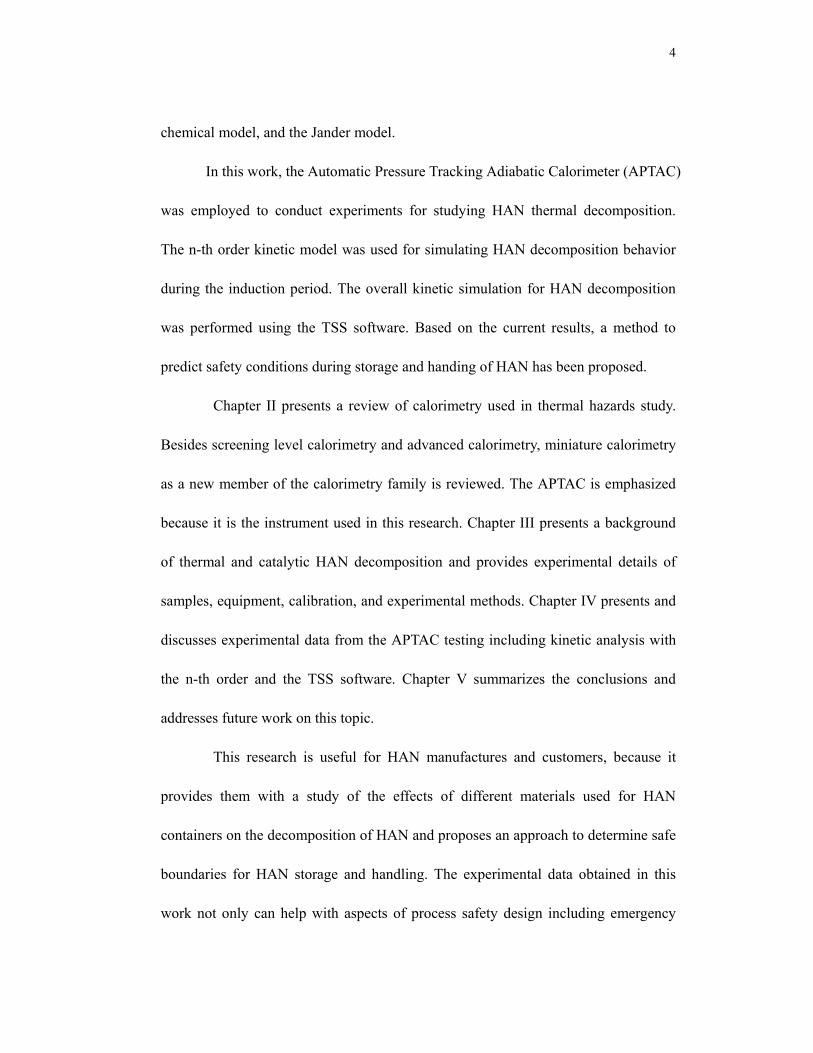
2.2.1. Differential Thermal Analysis (DTA)

Differential Thermal Analysis is a “fingerprinting” technique. It can provide

information on chemical reactions, phase transformations, and structure changes for a

sample under study. Usually, it connects a voltmeter with two thermocouples, which

are placed in a reference material (inert substance) such as Al2O3 and a sample

material, respectively. When the sample and reference material are subjected to an

identical temperature scanning program, temperature differences between them are

monitored as functions of temperature or time (CCPS, 1995). The principle of DTA is

that the input energy will steadily raise the temperature of the reference material,

which will be converted to latent heat during a phase transition of the sample. Figure

2.1 below shows a DTA instrument from Orton Instruments.

9

Fig.2.1. DTA from Orton Instruments (http://www.ortonceramic.com/instruments/pdf/DTA.pdf)

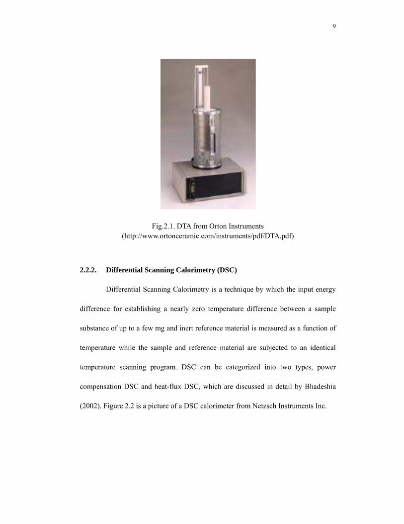
2.2.2. Differential Scanning Calorimetry (DSC)

Differential Scanning Calorimetry is a technique by which the input energy

difference for establishing a nearly zero temperature difference between a sample

substance of up to a few mg and inert reference material is measured as a function of

temperature while the sample and reference material are subjected to an identical

temperature scanning program. DSC can be categorized into two types, power

compensation DSC and heat-flux DSC, which are discussed in detail by Bhadeshia

(2002). Figure 2.2 is a picture of a DSC calorimeter from Netzsch Instruments Inc.

10

Fig.2.2. DSC-404C Pegasus® (http://www.e-thermal.com/dsc404c.htm)

2.2.3. Reactive System Screening Tool (RSST)

The Reactive System Screening Tool developed by Fauske & Associates is a

near-adiabatic calorimeter that characterizes reaction thermal nature rapidly with a

single heating scan. The sample substance is placed in a small open glass cell (about

10mL) that is contained in a stainless steel vessel pressurized with nitrogen. The

resulting RSST data yield rates of temperature and pressure rise due to runaway

reaction, which provides information about exothermic reactions and design

emergency relief devices (Fauske, 1993). The RSST is not very sensitive and can

only detect self-heat rates higher than 1oC/min. However, it is frequently used for

screening reactive chemicals due to its relative affordable price and ease of use. The

RSST and its control unit are shown in Figure 2.3.

11

Fig.2.3. RSST including a pressure vessel and control unit

(http://www.chem.mtu.edu/~crowl/rsst.htm)

The Advanced Reactive System Screening Tool (ARRST), based on the RSST,

is also manufactured by Fauske & Associates. Retaining the easy-to-use and

inexpensive characteristics of the RSST, the ARSST adopts new Windows software,

which adds many features such as wider scan rates (0~30oC/min), a heat-wait-search

(HWS) heating mode, and isothermal operation at elevated temperatures. As a result,

the sensitivity of onset detection is increased down to 0.1oC/min. A detailed

introduction of the ARSST was presented by Burelbach (2000).

2.2.4. Thermogravimetric Analysis (TGA)

Thermogravimetric Analysis is a technique for studying thermal stability of

chemicals in which the weight loss percentage of a sample is measured as a function

of temperature or time while the sample is being heated at a fixed rate. Information

about the composition of the sample is indicated by the mass loss during a specific

12

temperature range. It is commonly used for determining material characteristics,

degradation temperature, and decomposition point of explosives. Many companies

produce TGA apparatus, such as Linseis, Mettler, Perkin Elmer, and TA Instruments.

A typical TGA apparatus is shown in Figure 2.4 below.

Fig.2.4. TGA

(http://www.ptli.com/testlopedia/tests/ TGA-E1131.asp)

2.2.5. Isoperibolic Calorimetry

Isoperibolic Calorimetry is used to investigate the thermal behavior of

exothermic reactions. In this type of calorimeter, a surrounding jacket is maintained

at constant temperature while the temperature of the sample cell and its bucket are

raised due to heat released by sample decomposition or combustion. Commercial

isoperibolic calorimeters include SEnsitive Detector of EXothermic processes

(SEDEX), SIKAREX, and RADEX, whose photo is shown in Figure 2.5.

13

Fig.2.5. RADEX cell (left), SEDEX cell (middle), and SIKAREX cell (right)

(http://www.systag.ch/e530tsc5.htm# Measuring_cells)

2.3. Advanced Calorimetry

Advanced calorimetry used for thermal safety study includes adiabatic

calorimetry and reaction calorimetry. Adiabatic calorimetry is designed to investigate

worst-case scenarios for exothermic reactions, which has been proven to be a good

way to evaluate thermal hazards of reactive chemicals under runaway conditions

since the dynamic data of runaway reactions is measured directly. Reaction

calorimetry investigates heat flow due to exothermic reaction by simulating real

process conditions. Reaction calorimetry belongs to the general class of isothermal

calorimetry that cannot measure the runaway data directly. Therefore, adiabatic

calorimetry is preferred for runway reaction studies.

Compared with screening level calorimetry, adiabatic calorimetry is not only

14

time-consuming and expensive but also requires more experiment and interpretation

skills. However, adiabatic calorimetry is usually employed as an available best

practice (ABP) to study the greatest reduction in risk for safety management. It

minimizes heat losses during operation by adjusting the surrounding temperature to

match the sample temperature, which simulates the worst-case scenario of a runaway

reaction. The kinetic and thermodynamic data obtained by adiabatic calorimeter can

be applied to build computer models of reaction kinetics and runaway simulations

(Grolmes & King, 1995; Townsend et al., 1995; Liaw et al., 2001). The resulting

information can be used to conduct consequence analysis in risk assessment.

Commonly used adiabatic calorimeters include the Accelerating Rate Calorimeter

(ARC), Automatic Pressure Tracking Adiabatic Calorimeter (APTAC), Vent Sizing

Package (VSP), Phi-tec, and Dewar flask. Hereinto, ARC and APTAC are discussed

in this section. For other adiabatic calorimeters, information can be found in the open

literature (Yue, 1994; Gigante et al., 2003; Nomen et al., 1995).

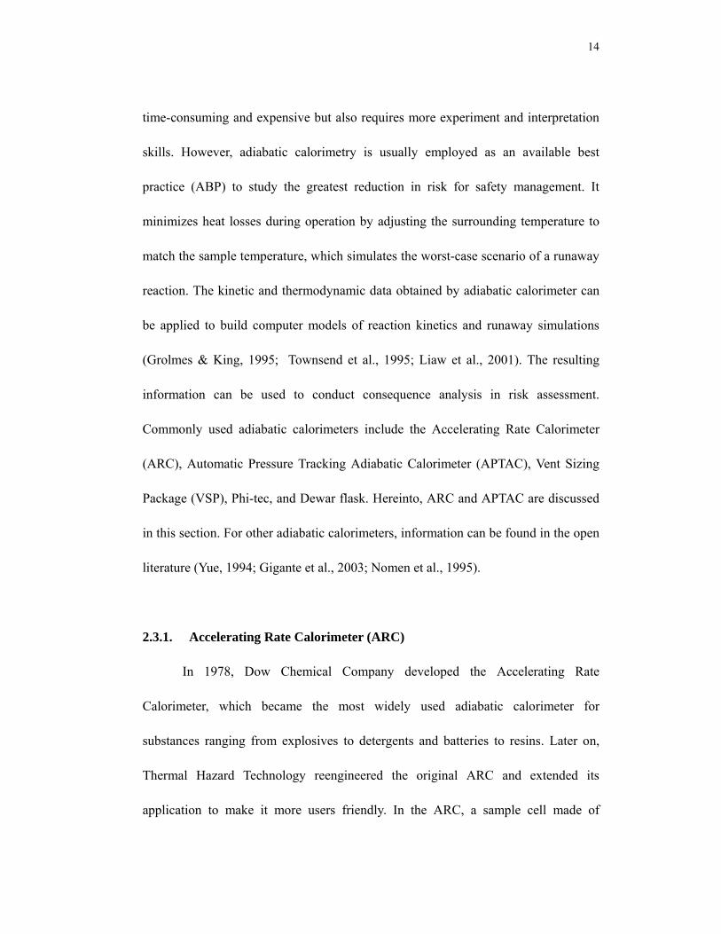
2.3.1. Accelerating Rate Calorimeter (ARC)

In 1978, Dow Chemical Company developed the Accelerating Rate

Calorimeter, which became the most widely used adiabatic calorimeter for

substances ranging from explosives to detergents and batteries to resins. Later on,

Thermal Hazard Technology reengineered the original ARC and extended its

application to make it more users friendly. In the ARC, a sample cell made of

15

stainless steel, titanium, tantalum, or Hastelloy is placed in an insulted container as

shown in Figure 2.6. Two heating modes (heat-wait-search and heating) are available

for the ARC. In the heat-wait-search mode, the ARC heats the sample material with a

fixed temperature increment, then switches to wait mode for stabilizing the

temperatures of the sample and containment vessel, and finally changes to a search

mode. If an exotherm is detected during the search mode, the ARC goes into the

adiabatic mode and follows the exotherm. Otherwise, it heats the sample material to

the next search stage at a higher temperature. For the heat mode, the sample material

is heated continuously until an exotherm is detected, and then the ARC switches to

the adiabatic mode to follow the exotherm.

The ARC can detect exotherms as low as 0.01oC/min. The operating

temperature can be up to 400oC and the pressure up to 200 bars. The data obtained

from ARC testing are temperature and pressure as functions of time, which are used

to calculate the maximum self heat rates, maximum pressure rates, onset

temperatures, and reaction kinetics parameters. The major problem with the ARC is

the high thermal inertia of the reaction vessel as a result of using a thick wall sample

cell and a relative small quantity of sample. Moreover, due to the limited cell heating

up to 20oC/min, the ARC is not appropriate to study under adiabatic conditions fast

exotherms such as some autocatalytic reactions.

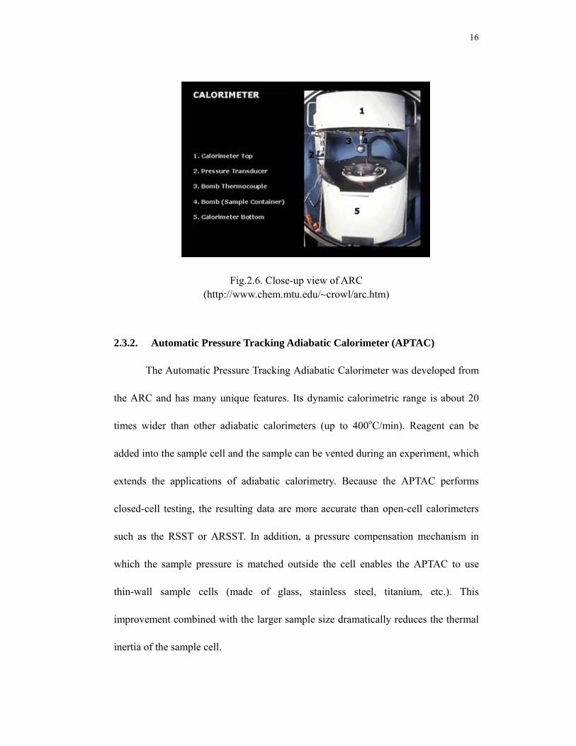
16

Fig.2.6. Close-up view of ARC (http://www.chem.mtu.edu/~crowl/arc.htm)

2.3.2. Automatic Pressure Tracking Adiabatic Calorimeter (APTAC)

The Automatic Pressure Tracking Adiabatic Calorimeter was developed from

the ARC and has many unique features. Its dynamic calorimetric range is about 20

times wider than other adiabatic calorimeters (up to 400oC/min). Reagent can be

added into the sample cell and the sample can be vented during an experiment, which

extends the applications of adiabatic calorimetry. Because the APTAC performs

closed-cell testing, the resulting data are more accurate than open-cell calorimeters

such as the RSST or ARSST. In addition, a pressure compensation mechanism in

which the sample pressure is matched outside the cell enables the APTAC to use

thin-wall sample cells (made of glass, stainless steel, titanium, etc.). This

improvement combined with the larger sample size dramatically reduces the thermal

inertia of the sample cell.

17

The APTAC is capable of studying exothermic reactions at temperatures

ranging from ambient to 500oC and pressures ranging from vacuum to 2000 psia. It

has various modes such as heat-wait-search, heat-soak-search, heat ramps, and

isothermal. Figure 2.7 is an overall view of APTACTM system, and Figure 2.8 is a

schematic of APTACTM pressure vessel.

Fig.2.7. Overall view of the APTACTM system

(http://www. calorimeters.net/Overview%20Products-Services/aptac.htm)

18

Fig.2.8. Schematic of the APTAC pressure vessel (Adapted from Wei, 2005)

Wall Thermocouple

19

2.4. Comparison of Calorimeters

No calorimeter can be used for all purposes because each one has its own

strengths and weaknesses based on the principle of measurement and range of

operation. Kersten et al. (2005) have conducted a Round-Robin test with

di-tertiary-butyl peroxide in the ARC, Phi-Tec, Pressure Dewar calorimeter (Dewar),

temperature controlled reactor (CRVM), and the APTAC for comparing the accuracy

and reliability of these adiabatic calorimeters. After these experiments, they

concluded that no specific type of equipment was superior to the others from an

overall point of view. However, if some requirements or limitations are specified, an

appropriate calorimeter may be selected for a specific application. A summary and

comparison of common calorimeters are listed in Table 1.1, which may help to

choose appropriate tools for specific studies of thermal hazards.

20Table 1.1. Comparison of commonly used calorimeters (Modified from http://www.harsnet.de/links/Calorimeters.htm) Calorimeter TSU Calwin DSC HP27 Radex Pressure range -1 to 60 bar Temperature range 0 to 400oC -20 to 200 oC Up to 750oC Typical sample size 5g 500g 1mg 2 to 10 mg 1 to 5 g (1 to 5 mL) Objective and method Thermal stability

screening Isoperibolic Isothermal test,

thermal stability screening

Thermal stability, high pressure DSC

Thermal stability screening method

Thermal sensitivity 1W/g <0.1mW/g ~3 µW/mg 1mW/g 5 J (0.1C x 50 J/C Heat Cap Radex)

Advantages* 1, 2, 3, 4, 7, 8 1,3,7 1, 2, 3 1, 2, 3, 8 1 (multiple tests at once), 3, pressure data

Disadvantages** 8 4, 8 4, 6, 8 1 (cleaning), 4, 5 Data obtained Onset temperature,

pressure ∆H, Cp, pressure ∆H, Cp, limited

kinetic data ∆H, kinetic data ∆H, relative onset

temperature Price Single test Low Low Low Low Medium Interpretation Low to medium Medium Medium Instrument Low to medium Low Medium Medium High Skills Experimentation Low Medium Medium Medium Medium Interpretation Medium to high Low High High High Manufacturer Hazard Evaluation

Laboratory Limited (HEL)

uniHH Netzsch Instruments Inc.

Mettler SYSTAG, System Technik AG

* Advantages: 1. Quick; 2. Only small sample needed; 3. Wide temperature range; 4. Sensitivity to T; 5. Low Phi-factor; 6. Accurate global kinetics; 7. Low price; 8. Small effort; 9. Other

**Disadvantages: 1. Time consuming; 2. Large sample required; 3. Restricted temperature range; 4. Insensitivity to T; 5. Medium/high Phi-factor; 6. More test runs needed; 7. Very expensive; 8. Cannot imitate process conditions; 9. Other

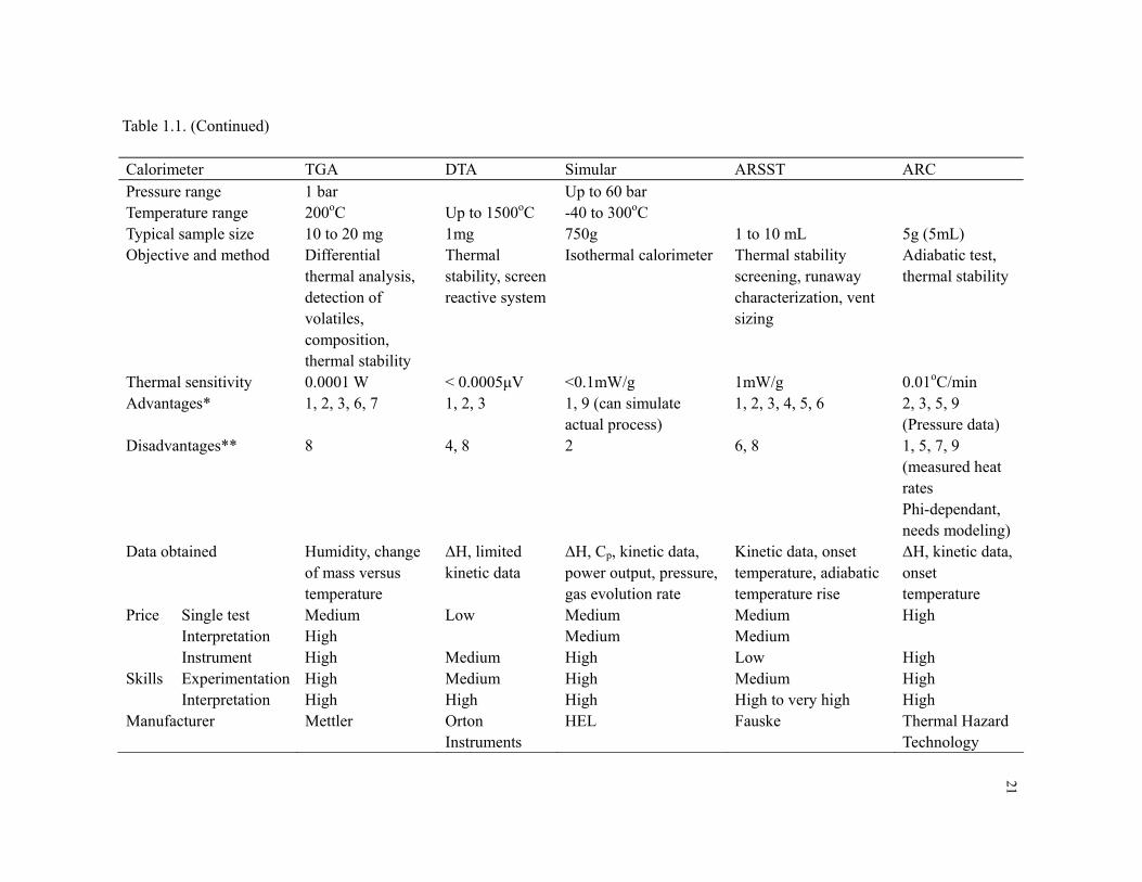
21Table 1.1. (Continued) Calorimeter TGA DTA Simular ARSST ARC Pressure range 1 bar Up to 60 bar Temperature range 200oC Up to 1500oC -40 to 300oC Typical sample size 10 to 20 mg 1mg 750g 1 to 10 mL 5g (5mL) Objective and method Differential

thermal analysis, detection of volatiles, composition, thermal stability

Thermal stability, screen reactive system

Isothermal calorimeter Thermal stability screening, runaway characterization, vent sizing

Adiabatic test, thermal stability

Thermal sensitivity 0.0001 W < 0.0005µV <0.1mW/g 1mW/g 0.01oC/min Advantages* 1, 2, 3, 6, 7 1, 2, 3 1, 9 (can simulate

actual process) 1, 2, 3, 4, 5, 6 2, 3, 5, 9

(Pressure data) Disadvantages** 8 4, 8 2 6, 8 1, 5, 7, 9

(measured heat rates Phi-dependant, needs modeling)

Data obtained Humidity, change of mass versus temperature

∆H, limited kinetic data

∆H, Cp, kinetic data, power output, pressure, gas evolution rate

Kinetic data, onset temperature, adiabatic temperature rise

∆H, kinetic data, onset temperature

Price Single test Medium Low Medium Medium High Interpretation High Medium Medium Instrument High Medium High Low High Skills Experimentation High Medium High Medium High Interpretation High High High High to very high High Manufacturer Mettler Orton

Instruments HEL Fauske Thermal Hazard

Technology

22Table 1.1. (Continued) Calorimeter Open Cup ARC VSP PHI-TECI APTAC Dewar Flask Pressure range Up to 1000 psia 0 to 138 bar Up to 2000 psia Temperature range -50 to 1000oC 0 to 500oC Up to 500oC -20 to 200oC Typical sample size 10g (20mL

Powder) 120mL (sample cell)

8g 130mL (sample cell) 200 to500 mL

Objective and method Adiabatic test, solids oxidative stability, storage stability

Adiabatic test, thermal stability

Adiabatic testing, thermal stability, runaway characterization

Adiabatic testing, thermal stability, runaway characterization

Adiabatic testing, thermal stability

Thermal sensitivity 0.01oC/min 0.05oC/min 0.02°C/min 0.04oC/min 0.5W/kg Advantages* 5, air flow at

elevated temperature,

3, 5, 9 (Pressure compensation)

1, 2, 3, 4, 6, 9 (Pressure compensation)

3, 5, 6, 9 (Pressure compensation)

3, 4, 5, 7, 9 (accurate data)

Disadvantages** 1, 2 1, 2 8 1, 7, 9 (measured heat rates Phi –dependant, needs modeling)

1, 2

Data obtained Kinetic data (zero order)

∆H, kinetic data, onset temperature, pressure

∆H, kinetic data, onset temperature, pressure

∆H, kinetic data, onset temperature, pressure, pressure

∆H, Cp, the induction time

Price Single test High High Medium High High Interpretation Medium Instrument High Medium High to very high Low Skills Experimentation High Medium Medium Medium Medium Interpretation High High High High Medium Manufacturer Fauske HEL TIAX

23

2.5. Miniature Calorimetry

With the development of nanotechnology and microfabrication, miniature

calorimetry as the new member in the calorimetry family has been gradually applied

in the area of process safety. Currently, miniature calorimetry used in safety studies

includes isothermal nanocalorimetry and isothermal microcalorimetry.

Isothermal nanocalorimetry is a technique based on similar principles such as

the DSC, but the calorimeter cell size is reduced to the micrometer or nanometer

scale. A commercialized isothermal nanocalorimeter (INC) developed by

Calorimeter Sciences Corp. (CSC) has been applied in measurement of

pharmaceutical shelf life, hazards evaluation of explosive storage, and the study of

chemical stability. This INC can detect a heat flow change as low as 1

nanocalorie/second. Such high sensitivity is a prerequisite for calorimetric study of

samples in limited quantity or with a hazardous nature. More information about the

INC is available on the website of Calorimeter Sciences Corp. (http://www.

calorimetrysciences.com/Calorimeters.html).

Isothermal microcalorimetry can monitor the heat flow generated by a

chemical, physical, or biological process as the sample is maintained at constant

temperature. The heat flow can be used to calculate the heat generated or consumed

by the sample placed in the calorimeter. Commercialized isothermal

microcalorimeters include the Tian-Calvet microcalorimeter and the Thermal

24

Activity Monitor (TAM).

The Tian-Calvet microcalorimeter is an isothermal microcalorimeter used for

the study of thermal decomposition including the determination of kinetics and the

evaluation and prediction of reaction progress. It can be used if the ARC indicates an

onset temperature of reaction within 50oC of the temperature required for the process.

Its sample size is 1~10mL compared with 100mL in the DSC. Moreover, the

Tian-Calvet microcalorimeter can obtain more accurate data than the usual DSC. A

detailed introduction to the Tian-Calvet microcalorimeter can be found on the

website of Setaram Instrumentation (http://www.setaram.com/).

The Thermal Activity Monitor was developed at the University of Lund

(Suurkuusk & Wadsö, 1982) and was commercialized by LKB Instruments in

Sweden. It is designed for detecting chemical activity that may develop into a

thermal runaway during storage or handling of bulk quantities. The third generation,

TAM III, allows multi-sample measurements to be performed simultaneously for up

to 48 hours. Its scanning mode can be set to less than 2oC/hr for an isothermal step.

The application of the TAM in the pharmaceuticals and biomaterials can be found in

the literature (Lechuga-Ballesteros et al., 2003; Zimehl et al., 2002).

2.6. APTAC Details

Because the APTAC is the instrument used in this research, detailed

information on its operation modes, data acquired, and general principles of

25

operation will be discussed under the following subtitles.

2.6.1. Operation Modes

The APTAC has several heating strategies for the sample including

heat-wait-search, heat-soak-search (also called iso-aging), heat-ramp by fixed

temperature difference, heat-ramp by rate, heat-ramp by rate with exothermal

detection, and isothermal. Heat-wait-search and heat soak-search are used in this

work. Information about the other strategies can be found in the control and

operation manual of the APTAC.

In the heat-wait-search, the APTAC heats the sample with a specified

temperature rate (say 2oC/min) to a starting temperature, then changes to wait mode

to allow for the temperatures of sample and containment vessel to stabilize, and

finally switches to search mode to detect exothermal behavior. During the process,

the self-heating rate of the sample is polled and compared with a predefined

sensitivity threshold. When the self-heating rate of the sample exceeds this threshold,

an exotherm is detected by the system. If an exotherm is detected during the search

mode, the APTAC will go into the adiabatic mode and follow the exotherm.

Otherwise, the sample material will be heated to the next higher predefined

temperature for the next exotherm search. The standard stabilization and searching

times are 25 minutes.

The iso-aging can be used to study the effects of inhibitors added to the

26

reactants. In this strategy, the sample material is heated first to a preset soak

temperature. The APTAC requires time for temperature stabilization of the pressure

vessel and sample (default value is 25 minutes) and then proceeds to the search

mode during which the APTAC maintains a constant sample temperature. During the

process, the self-heating rate of the sample is polled and compared with a predefined

sensitivity threshold. When the self-heating rate of the sample exceeds this threshold,

an exotherm is detected by the system. If an exotherm is detected in the search mode,

the APTAC will automatically switch to the adiabatic mode and follow the exotherm.

Otherwise, the APTAC will stay in the search mode until the predefined soak time is

ended and then proceed to a standard heat-wait-search.

2.6.2. Data Acquired

The data measured directly by the APTAC includes elapsed time, sample

temperature, reaction vessel temperature, containment vessel temperature, sample

pressure containment pressure, sample self-heating rate, and pressure rate of sample.

Important data curves that can be obtained from the APTAC software are

temperature versus time, pressure versus time, temperature versus pressure, heat rate

versus temperature, and pressure rate versus temperature profiles. These data and the

shapes of the curves can provide information about potential hazards posed by the

reaction that occurred in the system. Moreover, there are some important parameters

that may be used for further kinetic analysis of runaway reactions or for simulation

27

during the design of safety-relief devices. Useful reaction characterization

parameters include:

Onset temperature (Ton): “the temperature at which a detectable temperature

increase is first observed due to a chemical reaction” (defined by CCPS,

1995). Its value depends on the sensitivity of the temperature measuring

equipment. Usually, the more the thermally sensitivity, the lower the

measured onset temperature. The onset temperature is important information

for safe storage and handing of hazardous materials. A safety margin used in

industry is 50oC or more above the onset temperature to prevent undesired

reactions.

Maximum adiabatic temperature (Tmax): the maximum value during an

exothermic process. Tmax is an important parameter for kinetic analysis of a

runaway reaction.

Maximum pressure (Pmax): the maximum value of pressure during an

exothermic process. The major risk posed by a runaway reaction is the

mechanical failure of reactor or container due to overpressure. The Pmax is

important also for the design of safety relief valves.

Maximum self-heating rate (dT/dtmax). This value is used in the design of

safety relief devices.

Maximum pressure rate (dP/dtmax). This value is used in the design of safety

relief devices.

28

Time to maximum rate (TMR): the time from the self-heating rate at the

onset temperature to the maximum self-heating rate. This time is used to

estimate the response time of an emergency system to avoid a runaway

reaction.

Noncondensed pressure: the pressure in the gas phase of a sample when the

system is cooled down after a runaway reaction has finished. This value is

useful for the thermodynamic simulation of runaway reactions.

2.6.3. General Principles of Operation

Townsend and Tou (1980) illustrated data interpretation with the n-th order

kinetics for the ARC. Because the APTAC has similar principles to the ARC, the

data interpretation for the ARC is also suitable for the APTAC. Those general

principles of operation are reviewed here.

For an exothermic reaction, a runaway situation may occur if the heat

generated from the reaction is greater than the heat removed by the cooling system.

This phenomenon can be explained by the fact that the rate constant of a reaction

increases exponentially with temperature. The Arrhenius equation gives a

quantitative expression for this event:

)/exp(0 RTEkk a−= (1)

where k is the rate constant, k0 is the frequency factor, Ea is the activation energy for

the chemical reaction, and R is gas constant. Actually, a more general form of the

29

constant rate has been proposed as (Townsend & Tou, 1980):

)/exp(0 RTETkk aj −= (2)

where j is 0 in the Arrhenius equation, 0.5 in collision theory, and 1 in absolute rate

theory. However, the term of Tj is overshadowed by the exponential factor, because

the latter has wider variation. To simplify the model, j is taken as 0 whenever

considering the rate constant.

If the reaction is assumed to occur with homogeneous and n-th order kinetics

for a single reactant A, the reaction rate law of gives the reaction rate in terms of the

rate constant, concentration of species, and the reaction order:

nA

AA kC

dtdCr −== (3)

where rA is the reaction rate of component A, k is the rate constant, n is the reaction

order, and C is the concentration of component A.

For an exothermic reaction under adiabatic conditions (e.g., in an adiabatic

calorimeter), the heat produced from the initial reaction will cause a rise in

temperature that will in turn expedite the rate of reaction as shown in equations (1)

and (3). This acceleration effect will lead the system to a maximum temperature and

consume the concentration of reactant. Therefore, the reaction rate is expected to

achieve a maximum value at a temperature peak and then decrease to zero at the end

of the reaction. During the process of exotherm, the concentration of the reactant at

any temperature or time is given by:

30

oF

ooF

F CT

TTCTTTTC **

∆−

=−−

= (4)

where Co is the initial concentration; C is the concentration at any temperature T, and

To and TF are the initial and final temperatures, respectively.

The overall reaction heat generated is expressed as:

TmCH V ∆=∆ (5)

where ∆H is the overall reaction heat in terms of enthalpy, m is the mass of the

sample, CV is the average heat capacity at constant volume of the reaction system

over the temperature range, and ∆T is the adiabatic temperature rise.

By differentiating equation (4), the self-heat rate dT/dt is obtained and then

substituted into equation (3):

1)( −∆∆

−= n

onF TC

TTT

kdtdT

(6)

If a pseudo kinetic constant k* is defined as the following:

TT

TTdtdTkCk

nFno

∆∆

−== −

)(

/* 1

(7)

a relationship between ln (k*) and 1/T can be derived by combining equations (1)

and (7):

)1()ln(*)ln( 01

TRE

kCk ano −= −

(8)

Given a correct reaction order, the ln (k*) versus 1/T plot should be a straight line

with slope of Ea/R and intercept of 01kCn

o−

. The activation energy Ea and the

31

frequency factor k0 for the Arrhenius equation can be calculated based on the slope

and intercept of the plot.

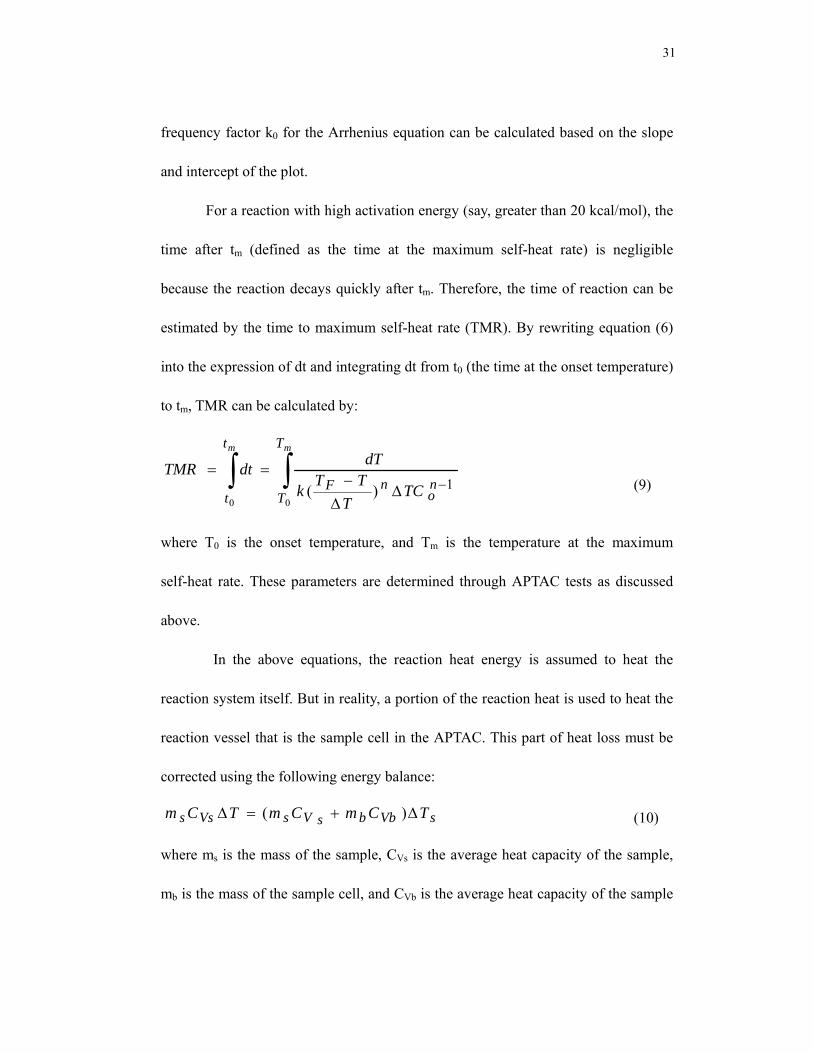
For a reaction with high activation energy (say, greater than 20 kcal/mol), the

time after tm (defined as the time at the maximum self-heat rate) is negligible

because the reaction decays quickly after tm. Therefore, the time of reaction can be

estimated by the time to maximum self-heat rate (TMR). By rewriting equation (6)

into the expression of dt and integrating dt from t0 (the time at the onset temperature)

to tm, TMR can be calculated by:

∫∫ −∆∆

−==

mm T

Tno

nF

t

t TCT

TTk

dTdtTMR

00

1)( (9)

where T0 is the onset temperature, and Tm is the temperature at the maximum

self-heat rate. These parameters are determined through APTAC tests as discussed

above.

In the above equations, the reaction heat energy is assumed to heat the

reaction system itself. But in reality, a portion of the reaction heat is used to heat the

reaction vessel that is the sample cell in the APTAC. This part of heat loss must be

corrected using the following energy balance:

sVbbsVsVss TCmCmTCm ∆+=∆ )( (10)

where ms is the mass of the sample, CVs is the average heat capacity of the sample,

mb is the mass of the sample cell, and CVb is the average heat capacity of the sample

32

cell, ∆T is the corrected adiabatic temperature rise, and ∆Ts is the adiabatic

temperature rise measured experimentally. If a new parameter called the thermal

inertia factor (φ) is defined as:

Vss

VbbVssCm

CmCm +=φ (11)

equation (10) can be written:

sTT ∆=∆ φ (12)

Commonly, 1/φ indicates the degree of adiabaticity of the calorimeter. For an

industrial runaway reaction under adiabatic surroundings, the φ factor approaches

and is generally equal to 1.

Considering the correction of φ, the adiabatic final temperature (TF) is:

sF TTT ∆+= φ0 (13)

Equations (4), (5), and (6) also become:

os

sFs CT

TTC *∆

−= (14)

sV TmCH ∆=∆ φ (15)

1)( −∆∆

−= n

osn

s

sFss

CTT

TTk

dtdT

(16)

where the subscript “s” indicates the measured value in an experiment.

33

CHAPTER III

EXPERIMENTAL DETAILS

3.1. Introduction

Hydroxylamine Nitrate (HAN), an important agent for the nuclear industry

and the U.S. Army, has been involved in several incidents. One major incident was

the 1997 Hanford explosion (U.S. Department of Energy, 1998). According to the

incident report from the U.S. Department of Energy (1998), the concentration of

HAN in aqueous solution had increased due to evaporation over the preceding four

years. and iron from the inner surface of the HAN container could have acted as a

decomposition catalyst. The higher HAN concentration, effect of iron contaminant,

and increased ambient temperature due to inadequate ventilation expedited the

violent decomposition of HAN.

Generally, HAN aqueous solution at relatively low HAN concentration up tp

24mass% is used in industries. It is a clear and odorless liquid. The molecular

formula of HAN is NH2OH·HNO3, and the gas phase structure of HAN is shown in

Figure 3.1. HAN is thermally unstable and can decompose autocatalytically at

elevated temperatures or in the presence of metal contaminants.

The kinetic mechanism of HAN decomposition has been investigated by

several groups (Dijk & Priest, 1984; Rafeev & Rubtsov, 1993; Schoppelrei & Brill,

1997; Oxley & Brower, 1988). However, no formalized kinetic modeling has been

34

developed to simulate HAN runaway behavior and predict its safe boundaries for

storage and handling. The major impediment is that HAN decomposition is an

autocatalytic reaction with a complicated reaction pathway. This research has

focused on the catalytic effects of stainless steel, titanium, and stainless steel with

titanium on the HAN decomposition, and developing a kinetic model for HAN

decomposition in storage tanks or other containers. Experiments were conducted

with the Automatic Pressure Tracking Adiabatic Calorimeter (APTAC).

Fig.3.1. Gas phase structure of HAN

(http://psc.tamu.edu/research/reactive chem_lab/HAN.htm)

This chapter presents experimental details on equipment, samples, methods,

and thermocouple calibration. In addition, background on the mechanism of HAN

reaction with nitrous acid, HAN thermal decomposition, HAN decomposition under

iron catalysis, and autocatalytic decomposition hazards are also provided.

35

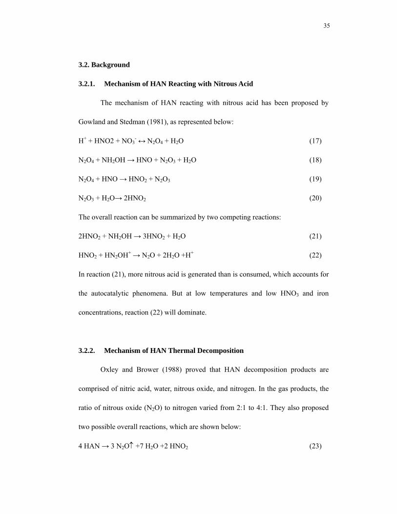
3.2. Background

3.2.1. Mechanism of HAN Reacting with Nitrous Acid

The mechanism of HAN reacting with nitrous acid has been proposed by

Gowland and Stedman (1981), as represented below:

H+ + HNO2 + NO3- ↔ N2O4 + H2O (17)

N2O4 + NH2OH → HNO + N2O3 + H2O (18)

N2O4 + HNO → HNO2 + N2O3 (19)

N2O3 + H2O→ 2HNO2 (20)

The overall reaction can be summarized by two competing reactions:

2HNO2 + NH2OH → 3HNO2 + H2O (21)

HNO2 + HN2OH+ → N2O + 2H2O +H+ (22)

In reaction (21), more nitrous acid is generated than is consumed, which accounts for

the autocatalytic phenomena. But at low temperatures and low HNO3 and iron

concentrations, reaction (22) will dominate.

3.2.2. Mechanism of HAN Thermal Decomposition

Oxley and Brower (1988) proved that HAN decomposition products are

comprised of nitric acid, water, nitrous oxide, and nitrogen. In the gas products, the

ratio of nitrous oxide (N2O) to nitrogen varied from 2:1 to 4:1. They also proposed

two possible overall reactions, which are shown below:

4 HAN → 3 N2O↑ +7 H2O +2 HNO2 (23)

36

3 HAN → N2O + N2↑+ 2 HNO3 +5 H2O (24)

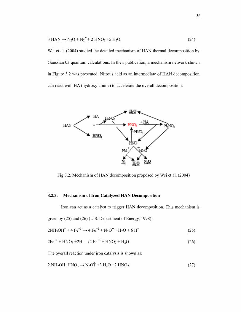
Wei et al. (2004) studied the detailed mechanism of HAN thermal decomposition by

Gaussian 03 quantum calculations. In their publication, a mechanism network shown

in Figure 3.2 was presented. Nitrous acid as an intermediate of HAN decomposition

can react with HA (hydroxylamine) to accelerate the overall decomposition.

Fig.3.2. Mechanism of HAN decomposition proposed by Wei et al. (2004)

3.2.3. Mechanism of Iron Catalyzed HAN Decomposition

Iron can act as a catalyst to trigger HAN decomposition. This mechanism is

given by (25) and (26) (U.S. Department of Energy, 1998):

2NH3OH+ + 4 Fe+3 → 4 Fe+2 + N2O↑ +H2O + 6 H+ (25)

2Fe+2 + HNO3 +2H+ →2 Fe+3 + HNO2 + H2O (26)

The overall reaction under iron catalysis is shown as:

2 NH2OH· HNO3 → N2O↑ +3 H2O +2 HNO2 (27)

37

According to Klein’s study (U.S. Department of Energy, 1998), in the presence of

iron the ratio of N2O to N2 in gas products for HAN decomposition was determined

to be 36:1. Therefore, compared to nitrous oxide, the amount of nitrogen produced is

negligible so it does not appear in the overall reaction (27).

3.2.4. Autocatalytic Decomposition Hazards

Autocatalytic reaction refers to a type of reaction that generates the catalyst

(or reactant) as a product. Autocatalytic reactions consist of three periods: induction,

explosion, and decay. During the induction period, the product that acts as a catalyst

is generated and accumulated. Once this catalytic product reaches a critical amount,

the explosion period starts and the temperature versus time curve exhibits a sharp

jump to approximately the maximum temperature. However, the explosion period

only lasts for a short time (may be less than a couple of seconds). After that, the

system enters the decay period due to the depletion of reactants. The rapid increase

in temperature and pressure during the explosion period poses a challenge to the

design of protection and mitigation measures relating to runaway reactions. The

existence of the induction period also poses a hazard for the extended storage for the

chemicals that undergo autocatalytic decomposition.

Dien et al. (1994) proposed a method to estimate the “time to maximum rate

under adiabatic conditions” (TMRad) for autocatalytic decomposition based on a

first-order reaction in competition with a Prout-Tompkins step, i.e. A→B, A+B→2B.

38

The kinetic parameters obtained from temperature-time curves in DSC testing can be

validated by ARC experiments. The TMRad calculated from the kinetic model is used

to determine the runaway time which can be used to plan corresponding

countermeasures.

Autocatalytic decomposition hazards can be measured and assessed using

general isothermal and adiabatic calorimeters. Bou-Diab and Fierz (2002) developed

a screening method based on dynamic DSC measurements to identify autocatalytic

decompositions. They found that autocatalytic decomposition occurred when the

apparent activation energy was higher than 220kJ/mol. A border value of the

apparent activation energy, 180-220kJ/mol, was suggested for use in screening

autocatalytic decomposition hazards. Wei et al. (2004) studied the autocatalytic

decomposition behavior of energetic materials using the APTAC. It has been proved

that APTAC can be a reliable and efficient screening tool to identify autocatalytic

decomposition hazards.

3.3. Experimental Details

3.3.1. Samples

Hydroxylamine nitrate (HAN) (24mass%) in aqueous solution purchased

from Aldrich (catalog number 438235), and an industrial HAN sample (17mass%,

aqueous solution) were used in this study without further purification and analysis.

The ppm concentrations of trace elements in the industrial HAN sample were

39

assumed to have negligible effect on the behavior of HAN decomposition.

Two kinds of materials, SS316 Ti and SS316, were used as catalysts to test

their effects on HAN decomposition. Before they were added to the glass cell the

catalysts were mechanically cut into bars. In order to obtain comparable results, the

surface areas of catalyst bars were designed to be equal (about 2.5 cm2).

3.3.2. Equipment

The experimental tests were carried out in the Automatic Pressure Tracking

Adiabatic Calorimeter (APTACTM) manufactured by TIAX, LLC. The APTAC is

capable of studying exothermic reactions with temperatures up to 500oC and

pressures up to 2000 psia in several testing modes (e.g., heat-wait-search, iso-aging,

isothermal, and heat ramps). The principle of the APTAC operation is to minimize

heat loss by adjusting the surrounding temperature to match the sample temperature.

This property is very useful in simulating the worst-case scenario of an industrial

runaway reaction. The APTAC can detect exotherms with a temperature rise rate of

0.04-400 oC/min and a pressure rise rate of 0.01-10,000 psia/min.

In the present work, a 100mL glass thick-wall cell, a 130mL titanium

thin-wall cell, and a 130mL stainless steel thin-wall cell were used as sample cells.

The surface area of the catalyst bar was measured by the 150mm dial caliper

(manufactured by Chicago Brand) before it was placed into the HAN sample. In

order to avoid contact of HAN with the metal sheath of thermocouple, a

40

Teflon-coated thermocouple (Omega part number OSK2K974/TJ8-NNIN-04OU-

12-PFA-SB-T-OTP-M) was used throughout the experiments.

3.3.3. Methods

The heat-wait-search (HWS) and the iso-aging modes were used in this work.

In the heat-wait-search, the sample was heated at 2oC/min until it reaches a

predefined starting temperature. Then the system changed to wait mode to stabilize

the temperature of sample and containment vessel and finally went to search mode to

detect an exotherm. Before an exotherm was detected, a default time of 25 minutes

was spent on each waiting or searching step. The threshold self-heating rate was

chosen as 0.05oC/min throughout the experiment. If the self-heating rate of the

sample exceeded this threshold during the search mode, the system automatically

entered the adiabatic mode and proceeded with the exotherm until the sample was

depleted or one of shutdown criteria was satisfied. Otherwise, the sample was heated

to the next higher predefined temperature for the next search.

In the iso-aging mode, the sample was heated to a preset soak temperature.

The APTAC took 25 minutes to stabilize the temperatures of the containment vessel

and the sample and then switched to search mode for soaking the sample at that

temperature. In this mode, the APTAC tracked the temperature of the sample to keep

the system isothermal. In this process, the self-heating rate of the sample was

compared with the predefined threshold (0.05oC/min). Once the self-heating rate of

41

the sample exceeded the threshold, the APTAC would automatically switch to

adiabatic mode and follow the exotherm. If no exotherm was detected during the

soak period, the APTAC would continue to proceed with a standard heat-wait-search.

The iso-aging mode is designed to study the effect of inhibitors or additives on

exothermic behavior of a sample material. In this work, the iso-aging mode was used

to test the effect of surrounding temperatures on the autocatalytic decomposition of

HAN.

Because the decomposition products of HAN in the liquid phase are water

and nitrous acid, sample cells were cleaned with deionized water first and then with

acetone before use. The same treatment was also applied to the catalyst bars before

they were placed into the HAN-water solutions. The Teflon-coated thermocouple

was flashed with deionized water and then acetone to remove contaminants from the

sheath surface before placing into the sample cell. The pressure unbalance criterion

was set at 80 psia for the glass cell and 100 psia for the titanium and stainless steel

cells. It was not necessary to use sample stirring in these tests because only a small

amount of HAN (several grams) was used in each experiment.

3.3.4. Thermocouple Calibration

Thermocouple (TC) calibration of the APTAC is necessary to maintain

accurate temperature measurements. There are two kinds of TC calibration: relative

and absolute. The relative calibration is used to make sure that the sample, cell wall,

42

and nitrogen thermocouples provide the same outputs if they are surrounded by the

same temperature, while the absolute calibration checks the accuracy of absolute

temperature of thermocouple measurements.

3.3.4.1. Relative Calibration

The adiabatic surrounding of the APTAC is obtained by adjusting the

nitrogen temperature to be approximately the same as the temperature of the sample.

Any deviation (negative or positive) between these two temperatures will cause

system error for the APTAC testing. The purpose of relative calibration is to

minimize either negative or positive drift of the system. It has been shown that 1oC

of deviation may cause a drift rate of 0.1oC/min at modest pressures. The higher the

pressure, the greater the drift rate for the same temperature difference (heat transfer

rate through the sample cell wall depends on the surrounding pressure). For an

exotherm detection level of 0.01oC/min, the thermocouples must be calibrated to

within 0.1oC or even less. Because the practical exotherm detection level changes

with pressure, the APTAC specifies its exothermal detection level as 0.04oC/min.

Whenever a sample cell or thermocouple is replaced, a relative calibration must be

done. Moreover, a schedule of relative calibration must be maintained. Normally, a

relative calibration is recommended every 10 runs.

An empty sample cell is usually used in a relative calibration. By selecting

“set up” on the menu bar and then choosing the “calibration” item, a dialog window

43

about calibration input data will be reached. A set of parameters (such as cooling

down temperature, ending temperature, operating pressure, heating rate, etc.) must

be input before starting a calibration. The starting temperature for calibration is

defaulted to 50oC. The ending temperature must be chosen within the normal

operating range of the thermocouple. For example, the Teflon-coated thermocouple

cannot withstand high temperature. Its working range is up to ~ 210oC. To ensure

that the 200oC point can be measured, 210oC may be chosen as the ending

temperature.

After the calibration is completed, a thermocouple offset versus temperature

curve is generated and stored automatically. This calibration curve covers the range

from –50oC to 500oC and records data every 50-degree interval. For the data that

cannot be obtained during calibration (-50oC, 0oC, 250oC, 300oC, 350oC, 400oC,

450oC, and 500oC for Teflon-coated thermocouple), the operator must manually

input the points by extrapolating from the measured calibration data and then

entering the data into the appropriate boxes in the Default Tabs 6 and 7. Figures 3.3

to 3.5 are the temperature-time curve, pressure-time curve, and thermocouple offset

profile, respectively, for the calibration of the Teflon-coated thermocouple (Omega

part number is OSK2K974/TJ8-NNIN-04OU-12-PFA-SB-T-OTP-M) in a glass cell.

Figure 3.6 shows the corresponding Default Tabs 6 and 7 for this calibration.

44

Fig.3.3. Temperature vs. time for the calibration test with initial

pressure at 300 psia

Fig.3.4. Pressure vs. time for the calibration test with initial pressure at 300 psia

45

Fig.3.5. Thermocouple offset vs. temperature profile

Fig.3.6. Default Tabs 6 and 7

46

3.3.4.2. Absolute Calibration

The thermocouple signal conditioning units in the APTAC system are set and

linearized for type N thermocouples. When a new type N thermocouple is placed into

an ice water mixture, if the reading is not 0oC, it is necessary to use the APTAC

software to adjust the zero point. Specifically, the nitrogen thermocouple is placed in

ice water and its offset from 0oC is recorded. This offset is entered into the

thermocouple offset data point in the Default Tab 2. Then the APTAC automatically

adds this value to all type N thermocouples, such as the sample, cell wall, and

nitrogen thermocouples.

47

CHAPTER IV

EXPERIMENTAL RESULTS AND DISCUSSION

4.1. HAN Decomposition in Glass Cell with SS316Ti or SS316

4.1.1. Objective

As mentioned in Chapter III, iron has a catalytic effect on hydroxylamine

nitrate (HAN) decomposition. In industry, stainless steel tanks (such as SS316Ti or

SS316) are used to store HAN in warehouses. Because it is a sensitive parameter for

the hydroxylamine family compounds, the effect of iron on HAN decomposition

must be investigated. A set of tests was designed to study catalytic effects of SS316Ti

and SS316 on HAN decomposition.

The HAN sample (24mass%) was purchased from Aldrich. A 100mL glass

cell was used as a sample cell in these tests because it can provide a relatively neutral

environment for HAN decomposition (Wei et al, 2004). Two materials, SS316Ti and

SS316, were used as catalysts. The SS316Ti material was provided by an industrial

company, and the SS316 material used in the tests was prepared by the chemical

engineering mechanical shop. Before being loaded into glass cell, the large pieces of

catalysts were cut into bars with surface areas of ~ 2.5cm2. HAN decomposition tests

in a glass cell without catalyst were also conducted. The APTAC heat-wait-search

mode was employed to study the exothermic behavior of HAN decomposition.

48

4.1.2 Results

The 24mass% HAN with no catalyst, with the SS316Ti catalyst bar, and with

the SS316 catalyst bar in the glass cell were examined by the HWS mode of the

APTAC and the experimental results are shown in Figures 4.1 to 4.4. Table 4.1

summarizes important parameters such as the onset temperature, maximum

temperature, maximum pressure, self-heating rate at onset temperature, maximum

self-heating rate, maximum pressure rise rate, non-condensable pressure at 50oC, and

reaction heat for each case. The presented uncertainties are within one standard

deviation based on three replicas. Phi factors and reaction heats (energies of reaction)

cannot be measured directly by the APTAC and were calculated using equations (11)

and (15) in Chapter II. The average heat capacity of HAN used in the thermal inertia

calculation was estimated to equal liquid water’s heat capacity (4.18 J/g/oC) because

it is not available in literature and water is a major product of decomposition. The

average heat capacity of titanium and stainless steel were estimated to be 0.544

J/g/oC and 0.5 J/g/oC, respectively (The references are given on the websites of

http://www.stanford.edu/~eboyden3/constants.html and http://www.lenntech.com/

Stainless-steel -316L.htm).

49

0

50

100

150

200

250

0 200 400 600 800 1000

Time (minutes)

Tem

pera

ture

(o C)

Glass cell onlyGlass cell with SS316Ti barGlass cell with SS316 bar

Fig.4.1. Temperature-time profiles of HAN (24mass%) decomposition in

a glass cell with/without catalyst

0

50

100

150

200

250

0 200 400 600 800 1000 1200Time (minutes)

Pres

sure

(psi

a)

Glass cell onlyGlass cell with SS316Ti barGlass cell with SS316 bar

Fig.4.2. Pressure-time profiles of HAN (24mass%) decomposition in

a glass cell with/without catalyst

50

0.001

0.01

0.1

1

10

100

1000

0 20 40 60 80 100 120 140 160 180 200

Temperature (oC)

Self-

heat

ing

rate

(o C/m

in)

glass cell onlyglass cell with SS316Ti barglass cell with SS316 bar

Fig.4.3. Self-heating rate-temperature profiles of HAN (24mass%)

decomposition in a glass cell with/without catalyst

0.001

0.01

0.1

1

10

100

1000

0 40 80 120 160 200

Temperature (oC)

Pres

sure

rate

(psi/

min

)

glass cell onlyglass cell with SS316Ti barglass cell with SS316 bar

Fig.4.4. Pressure rate-temperature profiles of HAN (24mass%)

decomposition in a glass cell with/without catalyst

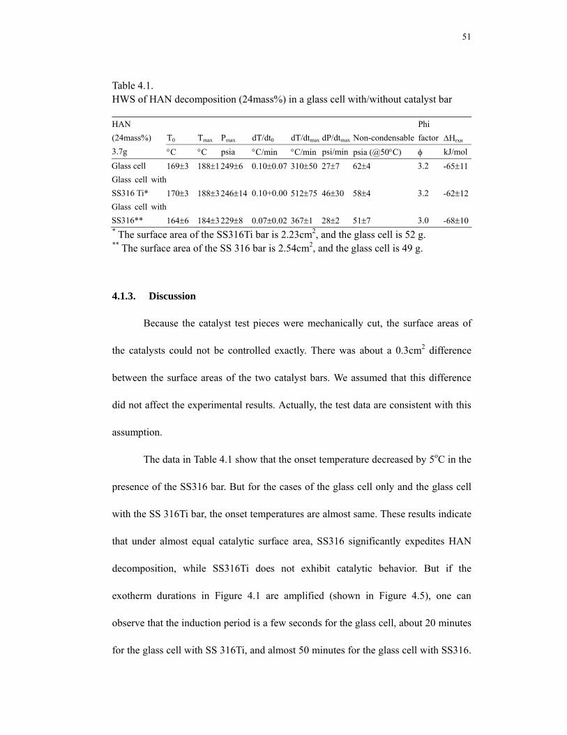
51

Table 4.1. HWS of HAN decomposition (24mass%) in a glass cell with/without catalyst bar

* The surface area of the SS316Ti bar is 2.23cm2, and the glass cell is 52 g. ** The surface area of the SS 316 bar is 2.54cm2, and the glass cell is 49 g.

4.1.3. Discussion

Because the catalyst test pieces were mechanically cut, the surface areas of

the catalysts could not be controlled exactly. There was about a 0.3cm2 difference

between the surface areas of the two catalyst bars. We assumed that this difference

did not affect the experimental results. Actually, the test data are consistent with this

assumption.

The data in Table 4.1 show that the onset temperature decreased by 5oC in the

presence of the SS316 bar. But for the cases of the glass cell only and the glass cell

with the SS 316Ti bar, the onset temperatures are almost same. These results indicate

that under almost equal catalytic surface area, SS316 significantly expedites HAN

decomposition, while SS316Ti does not exhibit catalytic behavior. But if the

exotherm durations in Figure 4.1 are amplified (shown in Figure 4.5), one can

observe that the induction period is a few seconds for the glass cell, about 20 minutes

for the glass cell with SS 316Ti, and almost 50 minutes for the glass cell with SS316.

T0 Tmax Pmax dT/dt0 dT/dtmax dP/dtmax Non-condensable Phi factor ∆Hrxn

HAN (24mass%) 3.7g °C °C psia °C/min °C/min psi/min psia (@50°C) φ kJ/molGlass cell 169±3 188±1 249±6 0.10±0.07 310±50 27±7 62±4 3.2 -65±11Glass cell with SS316 Ti* 170±3 188±3 246±14 0.10+0.00 512±75 46±30 58±4 3.2 -62±12Glass cell with SS316** 164±6 184±3 229±8 0.07±0.02 367±1 28±2 51±7 3.0 -68±10

52

This implies that SS316Ti does catalyze HAN decomposition because the induction

period exists but is weaker than SS316 with this amount of surface area. For the case

of the glass cell only, it is reasonable to assume that the glass material provides a

neutral test environment. In order to confirm the catalytic effect of SS316Ti, the

surface area of SS316Ti should be increased in future studies.

165

170

175

180

185

190

195

550 600 650 700 750 800 850 900 950

Time (minutes)

Tem

pera

ture

(o C

)

glass cell onlyglass cell with SS316Ti barglass cell with SS316 bar

Fig.4.5. Temperature-time behaviors of the exotherm durations in Fig. 4.1

The overall reaction heats (shown in Table 4.1) are close for the three cases.

This result suggests that an overall reaction thermal energy does not change in the

presence of a catalyst, which is not surprising because a catalyst only changes the

53

reaction pathway, not the overall reaction.

The thermal decomposition of HAN is an autocatalytic reaction that includes

an induction period, explosion period, and decay period. The maximum rates of

self-heating and pressure rise for HAN decompositions vary. This variation is partly

because the exotherm in the explosion period is so fast that the APTAC at its

measurement rate misses some of the critical data points. As shown in Chapter III,

the mechanism of this reaction is complicated because many intermediates are

generated and can react with each other. Without further analyzing the composition

and concentration of all important intermediates, it is very difficult to model the

whole decomposition process. However, for the safe storage and handling study, our

interest focuses only on the induction period, because the goal of this study is to

prevent rapid HAN decomposition from the beginning by addressing HAN storage in

tanks or containers before it exceeds its safety threshold.

According to the general principles of the APTAC described in Chapter II, a

relationship between ln (k*) and 1/T is given by:

)1()ln(*)ln( 01

TRE

kCk ano −= −

Given a correct reaction order, the ln (k*) versus -1/T plot should be a straight line

with a slope of Ea/R and an intercept of 01kCn

o−

. The overall activation energy Ea

and the frequency factor k0 in the Arrhenius equation can be calculated based on the

slope and intercept of the plot.

54

To simplify the problem, the first order kinetic model was used to represent

the experimental data for the induction period in these three cases. Figures 4.6, 4.7,

and 4.8 show kinetic analysis of HAN decompositions in the glass cell with/without

catalyst. It can be observed that the first order kinetic model (linear fitting of ln(k*)

vs. -1000/T) matches the experimental data very well. In these figures, the slope of

the fit line corresponds to Ea/R and the intercept of the fit line corresponds to ln(k0).

Ea and k0 are estimated and listed in Table 4.2.

y = 60.04x + 129.62R2 = 0.9986

-5.75

-5.5

-5.25

-5-2.25 -2.248 -2.246 -2.244 -2.242

-1000K/T

ln(k

*min

)

Experimental dataFit line

Fig.4.6. Kinetic analysis of HAN (24mass%) decomposition in

a glass cell without catalyst

55

y = 62.077x + 134.01R2 = 0.9952

-6.5

-5.5

-4.5

-3.5-2.26 -2.25 -2.24 -2.23 -2.22

-1000K/T

ln(k

*min

)

Experimental dataFit line

Fig.4.7. Kinetic analysis of HAN (24mass%) decomposition in

a glass cell with SS316Ti bar

y = 49.601x + 106.87R2 = 0.9952

-8

-6

-4

-2

0-2.28 -2.27 -2.26 -2.25 -2.24

-1000K/T

ln(k

*min

)

Experimental dataFit line

Fig.4.8. Kinetic analysis of HAN (24mass%) decomposition in

a glass cell with SS316 bar

56

Table 4.2. Summary of kinetic parameters of HAN (24mass%) in a glass cell with/without catalysts 1st order kinetics Ea (kJ/mol) k0 (min-1) Glass cell 499 1.9*1056 Glass cell with SS316Ti bar 516 1.6*1058 Glass cell with SS316 bar 412 2.6*1046

As mentioned above, SS316 shows a significant catalytic impact on the HAN

decomposition compared with SS316Ti. This can be explained from the apparent

overall activation energies listed in Table 4.2. The glass cell with the SS316 bar has

the lowest value for apparent activation energy. Therefore, it is possible that a

SS316Ti tank is superior to a SS316 tank for 24mass% HAN storage.

4.2. HAN Decomposition in Glass, Titanium, and Stainless Steel Cells

4.2.1. Objective

In the previous section, we suggested increasing the surface area of the

SS316Ti catalyst for further studies. However, the size of catalyst used in this

experiment was limited by the amount of HAN. Only a small amount of HAN can be

used in a test since HAN decomposition is rapid. If a larger amount of HAN is used,

the APTAC may not be able to follow the reaction adiabatically. Therefore, HAN

decomposition in sample cells of SS316Ti and SS316 can be used for increasing the

catalyst surface area for a small amount of HAN. A titanium sample cell instead of a

SS316Ti cell was employed because the latter was not available from TIAX, LLC or

57

other sources. A series of tests was conducted in glass, titanium, and stainless steel

cells to study the catalytic effect of iron and titanium on HAN decomposition.

The HAN sample (17mass%) was provided by an industrial company. The

titanium and stainless steel cells had a volume of ~130mL (standard) and the glass

cell had a volume of ~100mL. The APTAC heat-wait-search mode was used for onset

temperature search in these tests.

4.2.2. Results

The experimental results of this set of parallel tests are presented in Table 4.3

and Figures 4.9 to 4.12. In Table 4.3, the uncertainties presented are within one

standard deviation based on three replicas.

Table 4.3. HWS of the industrial HAN (17mass%) decomposition in different cells

T0 Tmax Pmax dT/dt0 dT/dtmax dP/dtmax Non-condensable Phi factor

∆Hrxn HAN (17mass%) 4.8g °C °C psia °C/min °C/min psi/min psia (@50°C) φ kJ/molGlass cell 169±2 191±4 255±24 0.06±0.04 8±4 94±89 62±3 3.1 -88±13Ti cell 158±3 176±1 182±5 0.06±0.01 246±40 12±3 42±1 1.9 -51±6 SS cell 148±3 167±4 158±11 0.06±0.04 4±0 20±5 45±1 2.4 -67±9

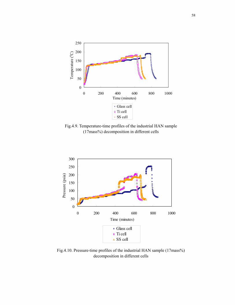
58

0

50

100

150

200

250

0 200 400 600 800 1000Time (minutes)

Tem

pera

ture

(o C)

Glass cellTi cellSS cell

Fig.4.9. Temperature-time profiles of the industrial HAN sample (17mass%) decomposition in different cells

0

50

100

150

200

250

300

0 200 400 600 800 1000Time (minutes)

Pres

sure

(psi

a)

Glass cellTi cellSS cell

Fig.4.10. Pressure-time profiles of the industrial HAN sample (17mass%) decomposition in different cells

59

0. 0010. 010. 1

110

1001000

0 50 100 150 200Temperature (oC)

Self-

heat

ing

rate

(o C/m

in)

Glass cellTi cellSS cell

Fig.4.11. Self-heating rate-temperature profiles of the industrial HAN

sample (17mass%) decomposition in different cells

0. 001

0. 01

0. 1

1

10

100

1000

0 50 100 150 200Temperature (oC)

Pres

sure

rate

(psi

/min

)

Glass cellTi cellSS cell

Fig.4.12. Pressure rate- temperature profiles of the industrial HAN sample (17mass%) decomposition in different cells

60

4.2.3. Discussion

In the temperature-time plot shown in Figure 4.9, the onset of self-heating of

HAN in the glass cell starts at about 170oC and continues to a maximum temperature

of 191oC. However, for the titanium or stainless steel cell, an obvious reduction in

onset temperature and maximum temperature for adiabatic rise is observed. Similar

trends are also displayed in the pressure-time behavior (shown in Figure 4.10).

The exotherm durations in Figure 4.9 are extracted and amplified in Figure

4.13. The induction periods are approximately 40 minutes for the titanium cell and 50

minutes for the stainless steel cell, and almost zero for glass cell. Therefore, the glass

cell offers a more neutral surrounding, while titanium and stainless steel catalyze

HAN decomposition. Moreover, these results suggested that stainless steel has a

stronger catalytic effect than titanium. From safety point of view, titanium or

stainless steel containing titanium should provide a more stable environment than

stainless steel for a HAN container material.

61

145

155

165

175

185

195

300 400 500 600 700 800 900

Time (minutes)

Tem

pera

ture

(o C)

Glass cellTi cellSS cell

Fig.4.13. Temperature-time behaviors of the exotherm durations in Fig. 4.9

Again, the first-order kinetic model was applied to fit the experimental data

for the induction period in all three cases. Figures 4.14 to 4.16 show kinetic analysis

of HAN decomposition in glass, titanium, and stainless steel cells. In the cases of

glass and titanium cells, the linear fit (first order kinetic model) matches

experimental data well. But for the case of stainless steel cell, the experimental data

display nonlinear behavior (Figure 4.16), which may be caused by a heterogeneous

catalytic reaction of HAN decomposition. See section 4.3.2. for more details.

62

y = 92.529x + 204.8R2 = 0.9746

-7.5

-6.5

-5.5

-4.5-2.28 -2.276 -2.272 -2.268

-1000K/T

ln(k

*min

)

Experimental dataFit line

Fig.4.14. Kinetic analysis of the industrial HAN sample (17mass%) decomposition in a glass cell

y = 40.432x + 88.507R2 = 0.9929

-6

-5.5

-5

-4.5-2.33 -2.32 -2.31 -2.3

-1000K/T

ln(k

*min

)

Experimental dataFit line

Fig.4.15. Kinetic analysis of the industrial HAN sample (17mass%)

decomposition in a titanium cell

63

y = 44.083x + 99.226R2 = 0.9881

-6.2

-5.7

-5.2

-4.7

-2.39 -2.38 -2.37 -2.36 -2.35

-1000K/T

ln(k

*min

)

Experimental dataFit line

Fig.4.16. Kinetic analysis of the industrial HAN sample (17mass%)

decomposition in a stainless steel cell

The apparent activation energies (Ea) and frequency factors (k0) for these

three cases can be estimated using the slopes and intercepts of the fit equations. Table

4.4 lists the values of Ea and k0. The stainless steel cell has greater value of Ea than

the titanium cell. This result seems not consistent with the previous conclusion that

stainless steel has a stronger catalytic effect than titanium. The stainless steel cell,

however, exhibits a typical heterogeneous catalysis on the HAN decomposition (see

section 4.3.2 for more details). However, n-th order kinetics was applied to analyze

the experimental data using perhaps an inaccurate assumption of homogeneous

reaction.

64

Table 4.4. Summary of kinetic parameters of the industrial HAN sample (17mass%) in different cells 1st order kinetics Ea (kJ/mol) k0 (min-1) Glass cell 769 8.8*1088 Titanium cell 336 2.8*1038 Stainless steel cell 366 1.2*1043

In Figure 4.17, the relationship between the reaction heat (∆Hrxn) and the

thermal inertial (φ) is linear. This means the total heat generated in the reaction for

the same amount of HAN is the same in the glass, titanium, and stainless steel cells.

As stated above, the catalytic effect of a container material only changes the reaction

pathway, not the overall reaction.

y = -30.78x + 7.2569R2 = 0.9997

-100

-80

-60

-401.5 2.5 3.5 4.5

φ

∆ Hrx

n

Fig.4.17. Linear relationship between φ and ∆Hrxn

65

4.3. Searching for Safe Boundary Conditions During HAN Storage and

Handling

In this study, the final objective is to predict safe boundary conditions for

HAN storage and handling. Usually, environmental temperature, HAN temperature,

tank pressure, and storage time can be observed or recorded easily for warehouse

storage and process handling. Therefore, predicting a safe boundary aims at defining

the safe threshold pressure and maximum safe storage time for an average storage

temperature.

There are two possible ways to predict the safe boundary of HAN storage.

One is an experimental approach. This requires the soak temperature to be as close as

possible to the ambient temperature of warehouse (since this temperature varies with

weather, season, and location, a conservative value such as 50oC can be adopted).

Given a certain soak time, the onset of exotherm behavior can be detected using an

appropriate instrument. However, the lower the soak temperature, the more soak time

that is needed to detect the exotherm. The other approach is simulation, i.e., a

combination of experimental work and kinetic simulation. If it is possible to develop

a validated kinetic-based model, a simulation under real storage conditions can be

generated and the associated safety boundary can be predicted.

66

4.3.1. Isothermal Aging Testing of the Industrial HAN Sample in a Stainless

Steel Cell

4.3.1.1. Objective

Although titanium or stainless steel containing titanium may be better than

stainless steel for a HAN container material, the research to find a safe boundary for

HAN storage in a stainless steel container is still attractive for HAN manufacturers

and customers, because titanium costs more than stainless steel.

Isothermal aging testing can be used to study the effect of inhibitors or

additives on exothermal behavior of a sample material. In this research, isothermal

aging testing was applied to test the effect of the aging factor on the autocatalytic

decomposition of HAN. Specifically, the trend of HAN autocatalytic decomposition

at different soak temperatures with varying soak times was determined during a

series of isothermal aging tests. This is a straightforward experimental approach,

because the safe storage time or pressure for a specific soak temperature (or

warehouse temperature) can be estimated by extrapolating from experimental data.

4.3.1.2. Results

The isothermal aging tests were performed using the industrial HAN sample

(17mass%) in a stainless steel cell (thin wall) with the APTAC iso-aging mode.

Because it is not practical to run experiments at lower temperature (such as 50oC)

67

due to extremely long testing times, parallel isothermal aging tests at higher

temperatures (120oC, 110oC, and 90oC) were performed with the soak times varied

from several hundred to a few thousand minutes. The important experimental

parameters are summarized in Table 4.5. As mentioned in Chapter II, if no exotherm

was detected in the soak stage, the system would convert to a standard

heat-wait-search, and an exotherm could be detected in this mode. Table 4.5 shows

that the exotherm was detected in the heat-wait-search mode for most cases. Only for

the run marked with a star was the exotherm detected during the soak stage. The

onset temperatures and pressures at various combinations of soak times and soak

temperatures are also shown in Figures 4.18 and 4.19. The behaviors of

temperature-time, pressure-time, self-heating rate-temperature, and pressure

rate-temperature for each test are included in the Appendix A.

68

Table 4.5. Iso-aging results of the industrial HAN decomposition in a stainless steel cell

* The exotherm was detected during the soak stage. Each listed value is the average value within three experimental replicas.

110

130

150

170

0 500 1000 1500 2000 2500Soak time (minutes)

Ons

et te

mpe

ratu

re (o C

)

Soak at 120 CSoak at 110 CSoak at 90 C

Fig.4.18. Onset temperature vs. soak time at various soak temperatures

Soak time T0 P0 Tmax Pmax dT/dt0 dT/dtmax dP/dtmax Non-condensableHAN (17mass%) 4.8g

min °C psia °C psia °C/min °C/min psi/min psia (@50°C)

Without soak 0 146 85 168 159 0.05 3.6 17 45 900 145 92 154 125 0.05 4.3 127 43 1,150 132 73 141 100 0.19 22 39 40

Tsoak=120oC

1,218* 124 63 143 108 0.05 42 35 45 1,000 131 74 166 168 0.05 26 184 54 Tsoak=110oC 1,200 121 63 143 108 0.05 26 34 45 900 141 86 170 179 0.05 19 1,018 53 1,500 137 78 159 142 0.05 15 201 47 2,000 141 86 158 135 0.08 5 235 43

Tsoak=90oC

2,500 136 79 153 123 0.05 6 153 44

69

40

60

80

100

0 500 1000 1500 2000 2500Soak time (minutes)

Ons

et p

ress

ure

(psia

)

Soak at 120 CSoak at 110 CSoak at 90 C

Fig.4.19. Onset pressure vs. soak time at various soak temperatures

4.3.1.3. Discussion

As expected, the overall trend is that the measured onset temperature

decreases with increasing soak time for any fixed soak temperature. But for the case

of soak at 90oC, it is difficult to observe a big difference in onset temperature for

soaking times within a few thousand minutes. When the industrial HAN sample was

soaked at 120oC, the lowest onset temperatures (124oC) was close to the environment

temperature (i.e. soak temperature) after a certain soak time. Since catalytic effect of

iron always exists for HAN stored in stainless steel tanks, this conclusion should also

be applied for lower temperatures such as ambient temperatures for warehouse

storage. Hence, there is a maximum safe storage time after which the onset of

decomposition will occur at environmental temperatures.

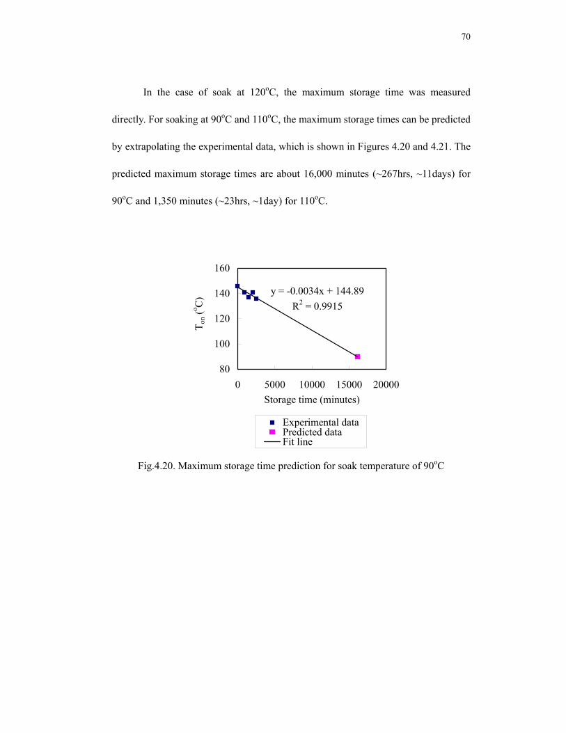
70

In the case of soak at 120oC, the maximum storage time was measured

directly. For soaking at 90oC and 110oC, the maximum storage times can be predicted

by extrapolating the experimental data, which is shown in Figures 4.20 and 4.21. The

predicted maximum storage times are about 16,000 minutes (~267hrs, ~11days) for

90oC and 1,350 minutes (~23hrs, ~1day) for 110oC.

y = -0.0034x + 144.89R2 = 0.9915

80

100

120

140

160

0 5000 10000 15000 20000Storage time (minutes)

T on (

o C)

Experimental dataPredicted dataFit line

Fig.4.20. Maximum storage time prediction for soak temperature of 90oC

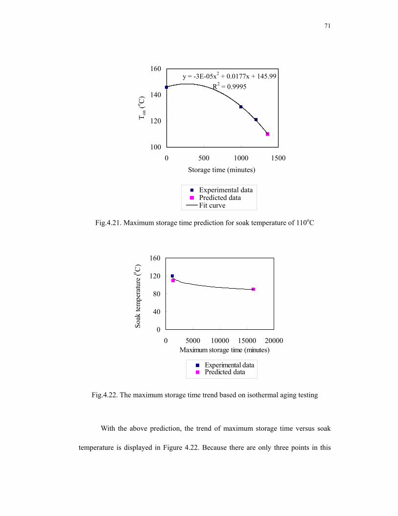
71

y = -3E-05x2 + 0.0177x + 145.99R2 = 0.9995

100

120

140

160

0 500 1000 1500Storage time (minutes)

T on (

o C)

Experimental dataPredicted dataFit curve

Fig.4.21. Maximum storage time prediction for soak temperature of 110oC

0

40

80

120

160

0 5000 10000 15000 20000Maximum storage time (minutes)

Soak

tem

pera

ture

(o C)

Experimental dataPredicted data

Fig.4.22. The maximum storage time trend based on isothermal aging testing

With the above prediction, the trend of maximum storage time versus soak

temperature is displayed in Figure 4.22. Because there are only three points in this

72

figure, many curves could be employed in a fit. However, provided sufficient

experimental data are collected over a sufficient range of decreasing temperature, the

maximum storage time at ambient temperature in a warehouse can, in principle, be

predicted.

Similar approaches can be employed to predict the onset pressure at

maximum storage time for each case. However, because the variation of pressure in

measurement is much larger than that of temperature for this reactive system, it is

more reliable to search for the threshold pressure for HAN safe storage by kinetic

simulation.

4.3.2. HAN Decomposition in a Stainless Steel Cell with Various Thermal

Inertias

4.3.2.1. Objective

In order to predict the safe threshold pressure during warehouse storage and

process handling of HAN, it is necessary to develop a kinetic-based model for its

autocatalytic decomposition. For this purpose, a set of tests for the thermal

decomposition of different masses of HAN was measured in a stainless steel cell.

4.3.2.2. Results

Different amounts of the industrial HAN sample (17mass%) in the same

stainless steel cell were examined using the heat-wait-search mode of the APTAC.

73

The experimental data are reported in Table 4.6. The behaviors of temperature vs.

time and pressure-time, self-heating rate-temperature, and pressure rate-temperature

are displayed in Figures 4.23 to 4.26. The exotherm parts in Figure 4.23 are extracted

and magnified in Figure 4.27.

Table 4.6. HWS results of thermal decomposition for different masses of the industrial HAN sample in a stainless steel cell

0

50

100

150

200

0 200 400 600 800Time (minutes)

Tem

pera

ture

(o C)

Phi=2.4 and mass=4.8gPhi=2.6 and mass=4.3gPhi=2.8 and mass=3.9g

Fig.4.23. Temperature-time profiles of the industrial HAN sample (17mass%) decomposition in a stainless steel cell

T0 P0 Tmax Pmax dT/dt0 dT/dtmax dP/dtmax Non-condensable Phi factor

∆Hrxn HAN (17mass%) in SS cell °C psi

a °C psia °C/min °C/min psi/min psia (@50°C) φ kJ/mol

4.8g (test 1) 146 85 168 159 0.05 3.6 17 45 2.4 76 4.3g (test 2) 146 83 167 155 0.05 5.2 76 43 2.6 77 3.9g (test 3) 146 86 163 140 0.05 3.7 15 38 2.8 73

74

0

50

100

150

200

250

0 200 400 600 800Time (minutes)

Pres

sure

(psia

)

Phi=2.4 and mass=4.8gPhi=2.6 and mass=4.3gPhi=2.8 and mass=3.9g

Fig.4.24. Pressure-time profiles of the industrial HAN sample (17mass%)

decomposition in a stainless steel cell

0.001

0.01

0.1

1

10

0 50 100 150 200Temperature (oC)

Self-

heat

ing

rate

(o C/m

in)

Phi=2.4 and mass=4.8gPhi=2.6 and mass=4.3gPhi=2.8 and mass=3.9g

Fig.4.25. Self-heating rate-temperature profiles of the industrial HAN sample

(17mass%) decomposition in a stainless steel cell

75

0.001

0.01

0.1

1

10

100

0 50 100 150 200Temperature (oC)

Pres

sure

rate

(psi

/min

)

Phi=2.4 and mass=4.8gPhi=2.6 and mass=4.3gPhi=2.8 and mass=3.9g

Fig.4.26. Pressure rate-temperature profiles of the industrial HAN sample (17mass%) decomposition in a stainless steel cell

145

150

155

160

165

170

360 385 410 435 460Time (minutes)

Tem

pera

ture

(o C)

Phi=2.4 and mass=4.8gPhi=2.6 and mass=4.3gPhi=2.8 and mass=3.9g

Fig.4.27. Temperature-time behaviors of the exotherm durations in Fig. 4.23

76

4.3.2.3. Discussion

An important observation from Figure 4.27 is that the induction period is

extended with an increase in sample mass. The shortest induction period corresponds

to the smallest sample amount. This is opposite of the normal homogenously

catalytic reaction in which the largest amount of sample has the shortest induction

period. Therefore, the HAN decomposition catalyzed by the inner surface of the cell

material is a typical heterogeneous reaction. Moreover, the higher ratio of contact

surface to sample mass contributes to a stronger catalytic effect due to a

heterogeneous interaction.

The kinetic simulation for heterogeneous reaction should be built on the

reaction mechanism. However, the mechanism of HAN heterogeneous catalytic

decomposition is not available in the literature. To simulate the kinetics of HAN

decomposition in a stainless steel cell, a pseudo-homogeneous reaction was assumed

in this work. Adiabatic Data Processing software (ADPro) and Formal Kinetics

Evaluation software (ForK) in the Thermal Safety Software package (developed by

ChemInform St. Petersburg Ltd.) were used for kinetic simulation of these three tests.

The full autocatalysis model was successfully applied to simulate the kinetics of

HAN decomposition in the stainless steel cell. The kinetic scheme is described

below:

A→B N-order (initiation stage) Equation: dα/dt = k0e -Ea/RT (1 - α) n

77

A→C Proto (autocatalytic stage) Equation: dα/dt = k0e -Ea/RT α n1 (1 - α) n2

where α is the degree of conversion of HAN (α is defined as (CA0-CA)/CA0; 0≤α≤1),

k0 is the frequency factor in the Arrhenius equation, n, n1, and n2 are reaction orders,

and Ea is the activation energy. The kinetic parameters for the initiation stage and

autocatalytic stage are reported in Table 4.7 and Table 4.8. The simulation results are

presented in Figure 4.28 to 4.30.

Table 4.7. Parameters of initiation stage (A→B) during HAN decomposition Parameters Units Value ln(k0) ln(1/sec) 33.48 Ea kJ/mol 151.42 n - 2.0 Q* kJ/kg 181.27

*Heat effects were calculated per unit of mass of the solution

Table 4.8. Parameters of autocatalytic stage (A→C) during HAN decomposition Parameter Units Test 1 Test 2 Test 3 ln(k0) ln(1/sec) 31.59 32.61 33.87 Ea kJ/mol 120.6 120.6 120.6 n1 - 4.0 4.0 4.0 n2 - 1.0 1.0 1.0 Q* kJ/kg 181.27 181.27 181.27 k0 1/sec 5.22*1013 1.46*1014 5.126*1014

*Heat effects were calculated per unit of mass of the solution

78

Fig.4.28. Simulation of test 1

Fig.4.29. Simulation of test 2

79

Fig.4.30. Simulation of test 3

As a result, the initiation stage of HAN decomposition was simulated by

second order kinetics, and the autocatalytic stage was simulated by the proto model

(the kinetic function is α n1 (1 - α) n2). The simulation curves shown in Figures 4.28

to 4.30 match the experimental data. Currently, this kinetic model cannot be used

directly for safe threshold pressure predictions. The model must be validated or

modified using additional experimental data. After a validated kinetic-based model is

developed, the simulation under real storage condition will be generated by the TSS,

and the safe threshold pressures before runaway can be estimated.

80

CHAPTER V

CONCLUSIONS AND FUTURE WORK

5.1. Conclusions

In this work, hydroxylamine nitrate (HAN) aqueous solution decomposition

in the presence of titanium, stainless steel with titanium, or stainless steel was

investigated with the Automatic Pressure Tracking Adiabatic Calorimeter (APTAC).

Titanium, stainless steel with titanium, and stainless steel exhibit catalytic effects on

the decomposition of HAN but their existence does not change the overall reaction

enthalpy of decomposition. Compared with stainless steel, titanium and stainless

steel with titanium are better choices for container materials during storage of HAN

aqueous solution.

An isothermal aging approach was proposed to predict the maximum storage

time of HAN. Sufficient experimental data could be used to predict the maximum

safe storage time of HAN at ambient temperature in these container materials.

A kinetics-based simulation was suggested to predict safe threshold pressures

for warehouse storage and process handling. First order kinetics was used to

represent the induction period data of HAN decomposition for initial estimation. In

the case of HAN decomposition in a stainless steel cell, a full autocatalysis model

was proposed to simulate the kinetics. Adiabatic Data Processing software (ADPro)

and Formal Kinetics Evaluation software (ForK) in the Thermal Safety Software

81

package were employed to perform this simulation.

5.2. Future Work

This work aims to find safe boundary condition for warehouse storage and

process handling of HAN aqueous solution. Additional work is needed to achieve the

final objective of this research, i.e., predictions of the maximum safe storage time

and the safe threshold pressure at ambient temperature.

First of all, a great deal of calorimetric data from the APTAC is required from

isothermal aging testing for reliable predictions of maximum HAN storage time. If

possible, calorimeters with higher thermal sensitivity should be used to conduct

experiments to increase the accuracy of testing. Secondly, the full autocatalysis mode

proposed to simulate HAN decomposition in a stainless steel cell must be validated

or modified by further experiments. In addition, the ratio of cell contact surface to

HAN mass is an important factor for this heterogeneous catalytic reaction. For

industrial storage, this ratio is much smaller than the ratio in experimental tests. For

example, if 2,000 pounds of HAN (24mass%) with a density of 1.118g/cm3 is stored

in a stainless steel tank with a 2.6ft inside diameter and a 5.3 ft height, the ratio of

contact surface to mass is about 0.05 cm2/g. But in the laboratory experiments, if

4.8g HAN used in a 130mL stainless steel cell, this ratio is about 2.4cm2/g. This is

almost 50 times greater than the ratio from the tank example. This difference must be

considered in scaling up predictions.

82

REFERENCES

Barreda, D. G. G., Vazquez, J., Lopez-Alemany, P. L., Villares, P., & Jimenez-Garay,

R. (2005). A comparative study on the glass-forming ability of some alloys in the Sb-As-Se system by differential scanning calorimetry. Journal of Physics and Chemistry of Solids, 66 (10), 1783-1787.

Bhadeshia, H. K. D. H. (2002). Differential scanning calorimetry. http://www. msm.cam.ac.uk/phasetrans/2002/Thermal2.pdf

Botros, S. H., Moustafa, A. F., & Ibrahim, S. A. (2006). Improvement of the homogeneity of SBR/NBR blends using polyglycidylmethacrylate-g-butadiene rubber. Journal of Applied Polymer Science, 99 (4), 1559-1567.

Bou-Diab, L., & Fierz, H. (2002). Autocatalytic decomposition reactions, hazards and detection. Journal of Hazardous Materials, 93 (1), 137-146.

Burelbach, J. P. (2000). Advanced reactive screening system tool (ARSST). 28th Annual Conference, North American Thermal Analysis Society. http://www. fauske.com/Download/Chemical/Papers/C29.pdf

Center for Chemical Process Safety (CCPS) (1995). Guidelines for chemical reactivity evaluation and application to process design. New York: AIChE, CCPS.

Dien, J-M., Fierz, H., Stoessel, F., & Kille, G. (1994). The thermal risk of autocatalytic decompositions: a kinetic study. Chimia, 48 (12), 542-550.

Dijk, C. A. V., & Priest, R. G. (1984). Thermal decomposition of hydroxylammonium nitrate at kilobar pressure. Combustion and Flame, 57 (1), 15-24.

Donoghue, E. (1997). Identifying hazardous chemical reactivity - a brief introduction. Journal of Thermal Analysis, 49 (3), 1609-1616.

83

Duh, Y.S., Hsu, C.C., Kao, C.S., & Yu, S.W. (1996). Applications of reaction calorimetry in reaction kinetics and thermal hazard evaluation. Thermochimica Acta, 285 (1), 67-79.

Fauske, H. K. (1993). U.S. Patent 5,229,074

Fauske, H. K. (2000). Properly size vents for nonreactive and reactive chemicals. Chemical Engineering Progress, 96 (2), 17-29.

Gigante, L., Lunghi, A., Martinelli, S., Cardillo, P., Picello, L., Bortolaso, R., Galvagni, M., & Rota, R. (2003). Calorimetric approach and simulation for scale-up of a Friedel-Crafts reaction. Organic Process Research & Development, 7 (6), 1079-1082.

Gowland, R. J., & Stedman, G. (1981). Kinetic and product studies on the decomposition of hydroxylamine in nitric-acid. Journal of Inorganic & Nuclear Chemistry, 43 (11), 2859-2862.

Grolmes, M. A., & King, M. J. (1995). Simulation of vented pressure-vessel tests for organic peroxides. Journal of Hazardous Materials, 44 (2-3), 253-266.

Gustin, J. L. (1993). Thermal-stability screening and reaction calorimetry-application to runaway reaction hazard assessment and process safety management. Journal of Loss Prevention in the Process Industries, 6 (5), 275-291.

Gustin, J. L., Fillon, J., Treand, G., & Elbiyaali, K. (1993). The phenol + formaldehyde runaway reaction – runaway reaction-vent sizing for reactor protection. Journal of Loss Prevention in the Process Industries, 6 (2), 103-113.

Kersten, R. J. A., Boers, M. N., Stork, M. M., & Visser, C. (2005). Results of a Round-Robin with di-tertiary-butyl peroxide in various adiabatic equipment for assessment of runaway reaction hazards. Journal of Loss Prevention in the Process Industries, 18 (3), 145-151.

Lechuga-Ballesteros, D., Bakri, A., & Miller, D. P. (2003). Microcalorimetric measurement of the interactions between water vapor and amorphous pharmaceutical solids. Pharmaceutical Research, 20 (2), 308-318.

84

Liaw, H. J., Chen, C. J., & Yur, C. C. (2001). The multiple runaway-reaction behavior prediction of MEK–oxidation reactions. Journal of Loss Prevention in the Process Industries, 14 (5), 371–378.

Lu, K. T., Luo, K. M., Lin, S. H., Su, S. H., & Hu, K. H. (2004). The acid-catalyzed phenol-formaldehyde reaction - Critical runaway conditions and stability criterion. Process Safety and Environmental Protection, 82 (B1), 37-47.

Maschio, G., Feliu, J.A., Ligthart, J., Ferrara, I., & Bassani, C. (1999). The use of adiabatic calorimetry for the process analysis and safety evaluation in free radical polymerization. Journal of Thermal Analysis and Calorimetry, 58 (1), 201-214.

Nomen, R., Sempere, J., Serra, E., & Pena, M. A. (1995). Safety subjects 5. Simple experiments to determine the thermal potential of a process: Adiabatic Dewar calorimetry. Afinidad, 52 (459), 291-295.

Oxley, J. C., & Brower, K. R. (1988). Thermal decomposition of hydroxylamine nitrate. Proceedings of SPIE-The International Society for Optical Engineering, 872, 63-70.

Rafeev, V. A., & Rubtsov, Y. I. (1993). Kinetics and mechanism of thermal decomposition of hydroxylammonium nitrate, Russian Chemical Bulletin, 42, 1811-1815.

Rota, R., Ruggeri, G., Morbidelli, M., & Ditali, S. (2002). Influence of calorimetric approximations on the design of emergency relief systems. Journal of Loss Prevention in the Process Industries, 15 (1), 49-61.

Schoppelrei, J. W., & Brill, T. B. (1997). Spectroscopy of hydrothermal reactions. 7. Kinetics of aqueous [NH3OH]NO3 at 463-523 K and 27.5 MPa by infrared spectroscopy. Journal of Physical Chemistry A, 101 (46), 8593-8596.

Sempere, J., Nomen, R., Serra, R., & Cardillo, P. (1997). Thermal hazard assessment using closed-cell adiabatic calorimetry. Journal of Loss Prevention in the Process Industries, 10 (1), 55-62.

Suurkuusk, J. & Wadsö, I. (1982). A multichannel micro-calorimetry system.

85

Chemica Scripta, 20 (4), 155-163

Townsend, D. I., & Tou, J. C. (1980). Thermal hazard evaluation by an acceleration rate calorimeter. Thermochimica Acta, 37 (1), 1-30.

Townsend, D. I., Freguson, H. D., Erguson, H. D., & Kohlbrand, H. T. (1995). Application of ARC(TM) thermokinetic data to the design of safety schemes for industrial reactors. Process Safety Progress, 14 (1), 71-76.

Tseng, J. M., Shu, C. M., & Yu, Y. C. (2005). Thermal hazard simulations for methyl ethyl ketone peroxide induced by contaminants. Korean Journal of Chemical Engineering, 22 (6), 797-802.

U.S. Chemical Safety and Hazard Investigation Board (2003). Hazard investigation: improving reactive hazard management. http://www.csb.gov/completed_ investigations/docs/ReactiveIncidentDataReport.pdf

U.S. Department of Energy (1998). Technical report on hydroxylamine nitrate. http://www.eh.doe.gov/chem_safety//Docs/hydroxlyamine.pdf

Wei, C., W. J. Rogers, & M. S. Mannan. (2004). Detection of autocatalytic decomposition behavior of energetic materials using APTAC. Proceedings of the 32nd North American Thermal Analysis Society Conference. Williamsburg, Virginia.

Wei, C. (2005). Thermal runaway reaction hazard and decomposition mechanism of the hydroxylamine system. PhD Dissertation, Texas A&M University, College Station, Texas.

Yue, M. H., Sharkey, J. J., & Leung, J. C. (1994). Relief vent sizing for a Grignard reaction. Journal of Loss Prevention in the Process Industries, 7 (5), 413-418.

Zimehl, R., Drews, J., & Fischer-Brandies, H. (2002). Thermometric monitoring of setting biomaterials. Thermochimica Acta, 382 (1-2), 161-168.

86

APPENDIX A

FIGURES OF ISOTHERMAL AGING TESTS OF

INDUSTRIAL HAN SAMPLE IN A STAINLESS

STEEL CELL WITH THE APTAC

Fig.A.1. Temperature as a function of time for soak temperature of 90oC and soak time of 900 minutes

87

Fig.A.2. Pressure as a function of time for soak temperature of 90oC and soak time of

900 minutes

Fig.A.3. Heat rate as a function of temperature for soak temperature of 90oC and soak

time of 900 minutes

88

Fig.A.4. Pressure rate as a function of temperature for soak temperature of 90oC and

soak time of 900 minutes

Fig.A.5. Temperature as a function of time for soak temperature of 90oC and soak

89

time of 1,500 minutes

Fig.A.6. Pressure as a function of time for soak temperature of 90oC and soak time of 1,500 minutes

90

Fig.A.7. Heat rate as a function of temperature for soak temperature of 90oC and soak time of 1,500 minutes

Fig.A.8. Pressure rate as a function of temperature for soak temperature of 90oC and soak time of 1,500 minutes

91

Fig.A.9. Temperature as a function of time for soak temperature of 90oC and soak

time of 2,000 minutes

Fig.A.10. Pressure as a function of time for soak temperature of 90oC and soak time of 2,000 minutes

92

Fig.A.11. Heat rate as a function of temperature for soak temperature of 90oC and

soak time of 2,000 minutes

Fig.A.12. Pressure rate as a function of temperature for soak temperature of 90oC and

soak time of 2,000 minutes

93

Fig.A.13. Temperature as a function of time for soak temperature of 90oC and soak

time of 2,500 minutes

Fig.A.14. Pressure as a function of time for soak temperature of 90oC and soak time

of 2,500 minutes

94

Fig.A.15. Heat rate as a function of temperature for soak temperature of 90oC and

soak time of 2,500 minutes

Fig.A.16. Pressure rate as a function of temperature for soak temperature of 90oC and

soak time of 2,500 minutes

95

Fig.A.17. Temperature as a function of time for soak temperature of 110oC and soak time of 1,000 minutes

Fig.A.18. Pressure as a function of time for soak temperature of 110oC and soak time of 1,000 minutes

96

Fig.A.19. Heat rate as a function of temperature for soak temperature of 110oC and soak time of 1,000 minutes

Fig.A.20. Pressure rate as a function of temperature for soak temperature of 110oC and soak time of 1,000 minutes

97

Fig.A.21. Temperature as a function of time for soak temperature of 110oC and soak

time of 1,200 minutes

Fig.A.22. Pressure as a function of time for soak temperature of 110oC and soak time

of 1,200 minutes

98

Fig.A.23. Heat rate as a function of temperature for soak temperature of 110oC and soak time of 1,200 minutes

Fig.A.24. Pressure rate as a function of temperature for soak temperature of 110oC and soak time of 1,200 minutes

99

Fig.A.25. Temperature as a function of time for soak temperature of 120oC and soak

time of 900 minutes

Fig.A.26. Pressure as a function of time for soak temperature of 120oC and soak time

of 900 minutes

100

Fig.A.27. Heat rate as a function of temperature for soak temperature of 120oC and

soak time of 900 minutes

Fig.A.28. Pressure rate as a function of temperature for soak temperature of 120oC

and soak time of 900 minutes

101

Fig.A.29. Temperature as a function of time for soak temperature of 120oC and soak time of 1,150 minutes

102

Fig.A.30. Pressure as a function of time for soak temperature of 120oC and soak time of 1,150 minutes

Fig.A.31. Heat rate as a function of temperature for soak temperature of 120oC and

103

soak time of 1,150 minutes

Fig.A.32. Pressure rate as a function of temperature for soak temperature of 120oC

and soak time of 1,150 minutes

Fig.A.33. Temperature as a function of time for soak temperature of 120oC, showing

104

the exotherm detected in the soak stage

Fig.A.34. Pressure as a function of time for soak temperature of 120oC, showing the

exotherm detected in the soak stage

Fig.A.35. Heat rate as a function of temperature for soak temperature of 120oC,

showing the exotherm detected in the soak stage

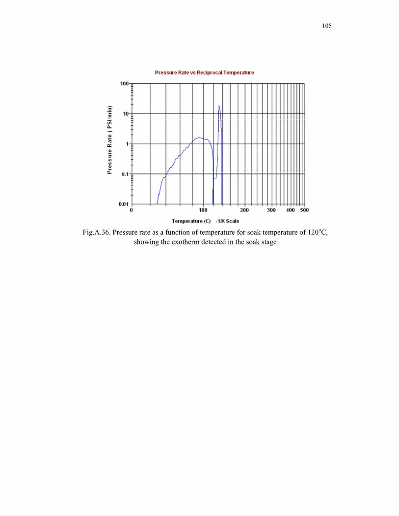
105

Fig.A.36. Pressure rate as a function of temperature for soak temperature of 120oC,

showing the exotherm detected in the soak stage

106

VITA

Chuanji Zhang was born in P. R. China in September 1978. She received her

B.S. degree in chemistry from Anhui Normal University in July 2000. In January

2003, she enrolled in the Science Majors Program in the Chemical Engineering

Department at Texas A&M University. In January 2004, she began work on her

master’s degree in the area of reactive chemicals. Her permanent address is:

Chaohu Middle Road #245, Room 502

Chaohu, Anhui

P.R. China, 238000.