Embed Size (px)
Citation preview

THERMAL CONDUCTIVITY OF SEDIMENTARY ROCKS -
SELECTED METHODOLOGICAL,
MINERALOGICAL AND TEXTURAL STUDIES.
by
Kirsti Midttemme
This thesis has been submitted
to
Department of Geology and Mineral Resources Engineering, Norwegian University of Science and Technology (NTNU)
in partial fulfilment of the requirements for The Norwegian academic degree
DOKTORINGEN10R
December 1997

DISCLAIMER
Portions of this document may be illegible in electronic image products. Images are produced from the best available original document.

1
SUMMARY.
The thermal conductivity of sedimentary rocks is an important parameter in basin modelling as the
main parameter controlling the temperature within a sedimentary basin. Measured thermal conductivities, mainly on clay- and mudstones, are presented in this work. The measured values
are compared with values obtained by using thermal conductivity models. Based on our
measurements some new thermal conductivity models are developed. The main findings of this
study can be summarised as follows:
Measured thermal conductivities.
• Thermal conductivities presented in this thesis are lower than most previously published data.
Divided bar measurements on four selected clay- and mudstones from England were in the range of 0.66 W/m-K to 0.97 W/m-K. For three of these clays, the measurements were less than half of the values previously published for the same clays.
• In a study of unconsolidated sediments, a constant deviation of about 0.15 W/m-K was found
between thermal conductivities measured with a needle probe and a divided bar apparatus. A similar disagreement between these two methods is also previously reported.
Modelling thermal conductivities.
• Accepted thermal conductivity models based on the geometric mean model, where matrix
conductivity is estimated from mineralogy, fail to predict the thermal conductivity of clay- and
mudstones.
• Despite this, models based on the geometric mean model, where the effect of porosity is taken
account of by the geometric mean equation, seem to be the best.• For clay- and mudstones the textural influence on thermal conductivity is underestimated by
existing models. This influence is considered to be the main reason for the unrealistic results with the mineralogically based models.
• The grain size was found to influence thermal conductivity for artificial quartz samples. This
effect seems to be logarithmic with highest effect for the fine grained samples.• The clay mineral content seems to be a point of uncertainty in both measuring and modelling
thermal conductivities.• In order to develop a good universal thermal conductivity model it is necessary to include many
mineralogical and textural factors. As this is difficult, different models restricted to specific
sediment types and textures are suggested to be the best solution to obtain realistic estimates applicable in basin modelling.

ii
PREFACE.
This thesis constitute the research project Shale and Claystones. Physical and Mineralogical
Parameters in Basin Modelling. This has been a part of the joint project Clay, Claystone and Shale
Problems in Petroleum Geology a co-operation between the Department of Geology and Resources Engineering, NTNU and the Department of Geology, University of Oslo.
What is the thermal conductivity of sedimentary rock? The most honest answer is still: «I do not
know.» When starting on this project the thermal conductivity was assumed to be one of many
parameters which would be touched on. Today, I am still studying this physical parameter called
thermal conductivity, and through these six years of thesis work I realise that a lot of work remains to obtain a satisfactory understanding of this parameter. In approaching an answer to the key question much attention has been paid to why we do not know the thermal conductivity of
sedimentary rocks better. A conclusion is unfortunately that the thermal conductivity is not only
influenced by the porosity, texture and mineralogy but also by whom and how the measurements
are carried out.
I would leave it to the readers and the dr.ing committee to evaluate the scientific contribution of
this work. My personal evaluation of this thesis period is that I have gone through some valuable
years where I have gained some insight in and respect for scientific methodology. I have also in
this period established a valuable network of contacts which has been both useful and pleasant and
which I hope is sustainable. Although this period of continuing education have been instructive, it
has certainly not been without times of adversity.

Ill
ACKNOWLEDGEMENTS.
Major economical funding was granted as scholarship from NFR, Norwegian Research Council as a part of the PROPETRO program (440.91/049). Statoil, Conoco N.I. and NTNU have also
financially supported this study. The work has been carried out at the Department of Geology and
Resources Engineering, NTNU.
I am indebted to the following people for their contributions in the process which resulted in this thesis:
• Elen Roaldset for her supervision and advise during this study. She is, together with Per Aagaard, leader of the joint project.
• 0istein Johansen, Oceanor, Willy Fjeldskaar, Rogaland Research, Mike Middleton, Chalmers University of Technology, Christian Hermanrud and Eirik Vik both Statoil, and Joar Sasttem, IKU for inspiring and useful discussions.
• Stephen Lippard for correcting and improving my English.• Helge Johansen, SINTEF Energi for measuring the thermal conductivities.
• Arne Hov, Karl Isachsen, Arild Monsoy, Ingrid Yokes and Ivar Ramme for technical support in
the laboratory work.
• Anne Irene Johannessen for drawing many of the figures.Thanks are also expressed to friends and colleagues at the Department of Geology and Mineral
Resources Engineering, NTNU for encouragement and help with all kinds of emerging problems. Finally I would honour my mother who encouraged me, but died during this period. As a good example I realise that she will influence choices I have to make also in the future.
Trondheim, October 1997. KlrtfiKirsti Midttemme
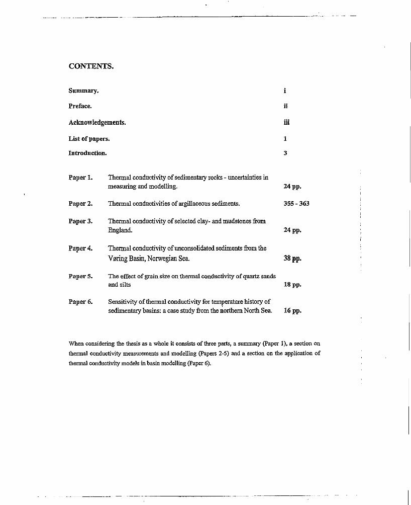
CONTENTS.
Summary. i
Preface. ii
Acknowledgements. in
List of papers. 1
Introduction. 3
Paper 1. Thermal conductivity of sedimentary rocks - uncertainties in measuring and modelling. 24 pp.
Paper 2. Thermal conductivities of argillaceous sediments. 355-363
Paper 3. Thermal conductivity of selected clay- and mudstones from England. 24 pp.
Paper 4. Thermal conductivity of unconsolidated sediments from the
Vering Basin, Norwegian Sea. 38 pp.
Paper 5. The effect of grain size on thermal conductivity of quartz sands and silts 18 pp.
Paper 6. Sensitivity of thermal conductivity for temperature history of sedimentary basins: a case study from the northern North Sea. 16 pp.
When considering the thesis as a whole it consists of three parts, a summary (Paper 1), a section on thermal conductivity measurements and modelling (Papers 2-5) and a section on the application of
thermal conductivity models in basin modelling (Paper 6).

1
LIST OF PAPERS.
Paper 1. Thermal conductivity of sedimentary rocks - uncertainties in
measuring and modelling.
Kirsti Midttomme & Elen Roaldset.
- In manuscript.
- Submitted to Mudrocks at the Basin Scale: Properties, Controls and Behaviour.
Geological Society Special Publications.
- Part of the paper entitled «Uncertaities in determination of thermal conductivity
of clay- and mudstones» was presented as a poster at Mudrocks at the Basin Scale: Properties, Controls and Behaviour. The Geological Society Meeting, London, January 1997.
Paper 2. Thermal conductivities of argillaceous sediments.Kirsti Midttomme, Elen Roaldset & PerAagaard.
- In: D.M. McCann, M. Eddleston, P.J. Penning & G.M. Reeves (eds.). Modem
Geophysics in Engineering Geology. Geological Society Engineering Geology
Special Publication, 12,355-363.
Paper 3. Thermal conductivity of selected clay- and mudstones from
England.
Kirsti Midttemme, Elen Roaldset & PerAagaard.
-In press. Clay Minerals, 33,131-145.
- Presented at The Rosenqvist Symposium on Clay Minerals in Modem Society, Oslo, May 1996.

2
Paper 4. Thermal conductivity of unconsolidated sediments from theVoting Basin, Norwegian Sea.
Kirsti Midttomme, Joar Scettem & Elen Roaldset.
- In press. In: M.F. Middleton (ed.). Nordic Petroleum Technology Series: Two,
Nordisk energiforskningssamarbejde, 1997.
- Part of the paper was presented and is published as abstracts in:
EAGE 57th Conference, Extended Abstracts Volume 2, F004 Glasgow, May
1995, ISBN 90-73781-06.
2nd Nordic Symposium on Petrophysics and Reservoir Modelling, Conference Volume, January 1996, 85-87.
Paper 5. The effect ofgrain size on thermal conductivity of quartz sands and silts.Kirsti Midttomme & Elen Roaldset.
- In press. Petroleum Geoscience.
- The paper was presented at 30th International Geological Congress, Abstracts Volume 1 of 3, H-2-29 04855 3702, pp 352, Beijing China, August 1996.
Paper 6. Sensitivity of thermal conductivity for temperature history of sedimentarybasins: a case study from the northern North Sea.Kirsti Midttomme & Willy Fjeldskaar.
- In manuscript.
- The paper will be presented at 23. Nordiske Geologiske Vintermode, Arhus,
January 1998.

3
INTRODUCTION.
GENERAL REMARKS.
Temperature.
All physical and chemical processes in nature depend on temperature. To know the temperature is
important in the understanding and the modelling of these processes. Equipment can be developed
which easily and exactly measures the temperature. However, for basin modelling purposes, this equipment is useless and therefore the temperature in sedimentary basins cannot be satisfactorily measured. The temperature within the basins has to be estimated. The thermal conductivity of the
sedimentary rocks filling the basin is a key parameter in these temperature models.
Basin modelling.
Basin modelling is a tool in the evaluation of the hydrocarbon potential of sedimentary basins. It is a young discipline within the broader subject of petroleum geology. The first integrated onedimensional basin models were presented at the end of the 1970s. Since then a variety of basin modelling tools and techniques has been developed, including in recent years also three- dimensional models (e.g.Hagemann, 1993).
Using basin modelling programs, the processes taking place within sedimentary basins, such as
heat and fluid flow, compaction, hydrocarbon generation, expulsion, secondary migration are modelled and the results of the processes integrated (e.g. Hermanrud, 1993). Still, the results of the modelling have to be considered with care because of the uncertainties and the inconsistencies in
the models, the input data and the calibration parameters. Basin modelling is important as a tool to
identify the sources of error in the modelling and the sensitivity of the parameters.
Why focus on the thermal conductivity?
The thermal conductivity is in itself of no interest in hydrocarbon generation or exploration. The interest in this parameter lies in its control of the temperature. Estimates of the temperature within
sedimentary basins require modelling of the heat transfer through the basins. The main mechanism
of heat transfer in sedimentary basins is by conduction. The principle of equilibrium underlies this
heat mechanism. If a temperature gradient exists in a material, heat transfer would try to even out
the temperature. The mechanism can physically be explained by transfer of energy from more energetic atoms and molecules to less energetic ones. A condition for conduction is contact between the particles.
4
The heat transfer due to conduction is expressed by Fourier’s law (eq.l).
(eq.l)
qkdT/dz
heat flux (W/m2),thermal conductivity (W/m-K),temperature gradient.
The heat flux, q, is the heat transfer in the z direction per unit area perpendicular to the direction of transfer, and is proportional to the temperature gradient, dT/dz in this direction. The proportional
constant, t is a transport property known as the thermal conductivity and is a characteristic of the
sedimentary rock (Incropera & Witt, 1990).
Heat is also transferred by other mechanisms such as convection and radiation. In this study the
heat contributions from these mechanisms are neglected. At temperatures lower than 250 °C heat
transfer from radiation is insignificant, particularly in fine grained sediments (e.g. Johansen, 1975; Midttemme et al., 1994).Whether there is a heat contribution from convection is more uncertain. The permeability is an important factor controlling convection. In this study I have mainly considered low permeable
rocks where the contribution from convection is considered to be minimal compared to conduction
(e.g. Ungerer et al., 1990). I have therefore considered to not take into account this contribution.
THESIS OUTLINE.
The thesis consists of six papers. Each paper represents a self contained work. When considering
the thesis as a whole, it consists of three parts, a summary (Paper I), several studies of thermal
conductivity measurements and modelling (Papers 2-5), and a study of the application of the
thermal conductivity models in basin modelling (Paper 6). A brief introduction and some comments to the papers follows:
Paper 1. Thermal conductivity of sedimentary rocks - uncertainties in measuring and
modelling.
Paper 1 is a review of this thesis and a summary of the five following papers. Also some new
statements and assumptions are presented. It might be seen as a confession of failure that this overview paper is entitled ((uncertainties in measuring and modelling* and discusses why we do

5
not know the thermal conductivity of sedimentary rocks. The paper is based on 6 years of thermal
conductivity studies and measurements with a divided bar apparatus carried out mainly on clays
and mudstones. Not all statements particular to measuring of thermal conductivities are well
examined or well-founded. By introducing these, I hope that further thermal conductivity studies can continue this work and confirm or deny these statements. The paper might suffer by the
restriction of the length. Instead of a thorough discussion of some main factors of uncertainties we
have tried to touch them all on a restricted number of pages.
Paper 2. Thermal conductivities of argillaceous sediments.
Paper 2 presents and discusses thermal conductivities measured on selected samples from the
Norwegian Continental Shelf. For basin modelling purposes these samples have great importance. However, the quality of the samples from well A is a point of uncertainty in this study. These samples were prepared from side wall cores contaminated with barite, where the interpretation of
the mineralogy and the determination of the direction due to the bedding were problematic.
Another problem with the samples from well A, is, although to the naken eye seeing rather
homogeneous, their very inhomogeneous nature (Figure 1 & 2). This paper might be marked by
being my first written paper. If it had been written today, more attention would have been given to
the textural factors of the samples. In relation to the following paper, this paper show trends in the
measuring of thermal conductivity, which form the basis for ideas and statements further developed in the following papers.
Paper 3. Thermal conductivity ofselected clay- and mudstones from England.
Thermal conductivities of four onshore clay- and mudstones from England are presented in Paper 3. The limited number of samples restricts the possibility to do statistical analyses of the thermal conductivity measurements and the laboratory data. The laboratory work carried out in this study is
more comprehensive and thorough than those presented in the other papers in this thesis, with
many parallel thermal conductivity measurements on each sample. A valuable part of this study is
the comparison between the needle probe, the divided bar, Middleton’s method, and those methods
previously published by Bloomer (1981).

6
Paper 4. Thermal conductivity of unconsolidated sediments from the Paring Basin,
Norwegian Sea.
The most comprehensive study is this thesis is presented in Paper 4. The young marine sediments studied here were obtain by gravity coring. For basin modelling purposes these samples are of
lower importance. The water content of these samples are extremely high compared to those
observed in more consolidated rocks. I believe that the study of these unconsolidated sediments has
given basic knowledge of heat transfer by conduction which also will give insight in this mechanism for more consolidated sediments. A weakness with this study might be that the samples are too homogenous. Comparative thermal conductivity measurements between needle probe method and the divided bar apparatus is also published in this paper. These measurements show a
rather constant deviation, where the divided bar apparatus give systematically lower values than the
needle probe method.
Paper 5. The effect ofgrain size on thermal conductivity of quartz sands and silts.
Paper 5 distinguishes itself from the other papers by treating artificial samples. By making the concession that natural samples are too complex to confirm a correlation between the grain size
and the thermal conductivity, moulded samples from crushed quartz were used. For the water
saturated samples a logarithmic correlation between the grain size and the measured thermal conductivities was found. The effect of pore size could possible have been more emphasised in this study. Since the grain size is found to affect thermal conductivity, the pore size is assumed to have
a corresponding effect.
Paper 6. Sensitivity to thermal conductivity for temperature history of sedimentary
basins: a case study from the northern North Sea.
The object of Paper 6 is to show how the variation in estimated thermal conductivity effects the
modelled temperature history of a sedimentary basin. This effect is exemplified by studying a
section across the northern North Sea. Thermal conductivities are estimated by six different methods, and four comparative case studies of temperature histories are considered. Since the
temperature history of this cross-section is unknown, the assessments of the different thermal
conductivity models are only based on assumptions. Considerable variations in the estimated temperature histories is observed.

7
Figures 1 & 2. Sample A7 in Paper 2. The sample is from Middle Eocene, The side wall core
(Figure 1) shows a dark grey mudstone. Drilling fluid contamination is seen as light spots on the surface. The thin section micrograph'(Figure 2) shows a sandy mudstone with Iithic fragments of
light brown claystone, quartzite and carbonate. !)
!

8
45cm j
1
Figures 3 & 4. Sample B3 in Paper 2 (Zhang
Heather Formation. The core section (Figure 3)
by bioturbation. The thin section micrograph
elongated mica minerals in a clayey matrix.
t 300pmt
et al., 1992). The sample is from Upper Jurassic
shows a mottled pattern. The bedding is modified
(Figure 4) shows silt-size quartz, feldspar and

9
MEASUREMENTS OF THERMAL CONDUCTIVITIES.
Thermal conductivities reported in this study are mainly measured with a divided bar apparatus,
developed at the Institute of Refrigeration, Norwegian University of Science and Technology
(Brendeng & Frivik, 1974). The reproducibility of repeated measurements with this apparatus on a
variety of rock samples is within 3.0 % (H. Johansen, pers. comm, 1992).
The measurements presented in this study were, except for some data in Paper 5, measured on
water saturated samples. All measurements were carried out at atmospheric pressure and at temperatures in the range 15 - 55 °C. To prevent drying of the samples and reduce the effect of
water movement, the temperature gradient across the samples was minimalized to 0.5 - 5.0 K. A
problem with measuring on water saturated material is drying as this will dramatically lower the
measured thermal conductivity. Examples of drying are shown for samples 123 and 200 in Paper 4, Figure 7. The effect of drying is also seen in Paper 5, Table 1 where thermal conductivities of synthetic quartz samples measured in both water saturated and dried condition are presented. The measured thermal conductivity of one of the samples (sample 20 -63 pm B) was reduced by 68 %
from originally 1.42 W/m-K to 0.45 W/m-K after drying. For some of the repeated measurements a
considerable reduction in the thermal conductivity was observed and related to drying. The values obtained after such reduction are not considered in this study.
During this study the reproducibility of the measurements has been tested. A distinction is made between experimental error and sample error (Davis, 1973). Experimental error reflects the uncertainty in the measurements by the divided bar apparatus itself. This error was found by
repeated measurements on selected samples under identical conditions (Table 1).
Table 1. Experimental errors as obtained by repeated measurements on selected samples.Presentedin thesis
Sample* MeasuredthermalconductivityW/m-K
Deviation%
Thesis study unpubl. Quaternary clay, Gauldal, TrsndelagSample size: 25.0-25.0-6.0 cm? 1.0022/1.0058 + 0.4Sample size: 15.0T5.0-3.0 cm3 1.3666/13883 +1.6Sample size: 5.0 5.0 3.0 cm3 0.8673 / 0.8472 -23
Papers Clay-/mudstones, England Sample size: cube, 1=3.0 cm London clay, LI, (parallel, 27 °C ) 1.1208/1.1483 +2.5Fullers Earth, Reigate, R2, (perpendicular, 27 °C) 0.7616/0.7552 -0.8Fullers Earth, Reigate R3, (parallel, 27 °C) 0.7660/0.7693 -0.4
Paper 4 Unconsolidated sediments, Voring Basin Sample size: cube, 1 =3.0 cmSample no. 186 (parallel, 46 °C) 0.882 / 0.862 -23Sample no. 200 (parallel, 41 °C) 0.728 / 0.728 0.0
Paper 5 Hydrothermal quartz Sample size: cube, 1 =3.0 cm Massive B (perpendicular, 25°C /31 °C ) 3.764/3.676 -23Massive B (parallel, 25°C / 31°C) 3.957 / 4.000 +1.1
* measured direction to the layering and the mean temperature of the sample during the run is given in parenthesis.

10
Sample errors reflect uncertainties in the measurements due to the sampling and sample
preparation process. This error was found by measuring parallel samples prepared from the most homogeneous material in this study (Table 2).
Table 2. Sample errors as obtained from measurements on parallel samples of the most homogeneous material in this study. The samples are cubes, 1 =3.0 cm.
Presented in thesis
Sample* Measured thermal conductivity W/m-K
Deviation%
Paper 3 Clay-/ mudstones, EnglandFullers Earth, Reigate, (perpendicular, 27 °C) 0.758 / 0.741/0.739 -0.9-+ 1.6
(parallel, 27 °C) 0.817/1.096/0.768 -14.1-+22.6Fullers Earth, Baulking (perpendicular, 27 °C) 0.711/0.682 / 0.660 - 3.6 - + 3.9
(parallel, 27 °C) 0.806/0.819/0.769 -3.6-+ 2.6Paper 5 Hydrothermal quartz
Massive sample (perpendicular, 25 °C) 4.217/3.720 -11.8(parallel, 25 °C) 4.295 /4.303 +0.2
* measured direction to the layering and the mean temperature of the sample during the run is given in paranthesis.
As seen in Tables 1 & 2 the experimental error was within 2.5 % for the tested samples while the
sample error was within 3.9 % for four of the six parallel measurements. For the parallel
measurements of Fullers Earth from Reigate and the perpendicular ones of the hydrothermal
quartz, sample errors of +22.6 % and 11.8 % respectively were detected. These high errors might
reflect inhomogenities in the material.
COMPARISON OF THERMAL CONDUCTIVITY MEASUREMENTS.
This study focus on the thermal conductivities of clays and clay- and siltstones. The measurements
reported in Paper 2 and in a separate study of sandy sediments from the Ness Formation, Oseberg field (Midttemme et al., 1996), are plotted together with thermal conductivity data included in a
commercial basin modelling program (confidential) and from McKenna et al. (1996) as a function of porosity (Figure 5). This figure shows that thermal conductivities measured in this study are
considerably lower than the data for pure sandstones. The thermal conductivity measurements
reported in Paper 2 are also slightly lower than data on shales from the Norwegian Shelf. It is noteworthy to point out that the Norwegian Shelf data were obtained by the needle probe
technique. A discrepancy due to the method of measurement is discussed in Papers 1, 3 & 4.
Methodological, mineralogical and textural factors which may explain the variation in thermal
conductivities seen in Figure 5, are discussed in Papers 1,2,3,4 & 5 in the thesis.

11
o
1 3,00 ■ ■
> 2,00
.O O o
20,00
Porosity
XSandstones, Norwegian Shelf
OShales, Norwegian Shelf
OSandstones, Frio and Wilcox Formation, Gulf of Mexico Basin, (McKenna et al., 1996)
) Argillaceous sediments, Norwegian Sea and North Sea, Paper 2
ASandy sediments, Ness Formation, Oseberg field, (Midttemme et al.,1996)
Figure 5. Comparison of measured thermal conductivities. Data from Norwegian Shelf is included
in a commercial basin modelling program and is statistically treated by Seter (diploma thesis, NTNU, in prep.).

12
REFERENCES.
Bloomer, J.R. 1981: Thermal conductivities of mudrocks in the United Kingdom. Quarterly
Journal of Engineering Geology, 14,357-362.
Brendeng, E. & P.E. Frivik, 1974: New develop ement in design of equipment for measuring
thermal conductivity and heat flow. Heat transmission measurements in thermal
insulations, ASTM SIP 544, American Society for Testing and Materials, p. 147-166.Davis, J.C. 1973: Statistics and Data Analysis in Geology. John Wiley & Sons, 550 pp.Incropera, F.P. & De Witt, D.P. 1990: Fundamentals of heat and mass transfer. Third edition. John
Wiley & Sons, 917 pp.
Hagemann, F. 1993: Preface. In: Ed: Dore, A,G et al.: Basin Modelling: Advances and
Applications. Norwegian Petroleum Society (NPF) Special Publication 3, Elsevier, Amsterdam, DC.
Hermanrud, C. 1993: Basin modelling techniques - an overview. In: Ed: Dore, A,G et al.: Basin
Modelling: Advances and Applications. Norwegian Petroleum Society (NPF) Special
Publication 3, Elsevier, Amsterdam, 1-33.Johansen, 0.1975: Varmeledningsevne avjordarter. Dr.ing avhandling, institutt for kjoleteknikk,
NTH, 231pp.
McKenna, T. E., Sharp, J. M. Jr., & Lynch, F.L. 1996: Thermal conductivity of Wilcox and Frio
sandstones in south Texas (Gulf of Mexico Basin). AAPG Bulletin, 80,1203-1215.Midttemme, K., E. Roaldset & P. Aagaard, 1994: Termiske egenskaper i sedimentcere bergarter,
Rapport fra institutt for geologi og bergteknikk, Norwegian University of Technology
(NTH), 29,94p.
Midttemme, K., Roaldset, E. and Brantjes, J.G. 1996: Thermal conductivity of alluvial sediments from the Ness Formation, Oseberg Area, North Sea. EAEG 58th Conference, Extended Abstracts Volume 2, P552, Amsterdam.
Ungerer, P., Bujtus, J., Doligez, B., Chenet, P.Y. & Bessis, F. 1990: Basin evaluation by integrated
two-dimensional modeling of heat transfer, fluid flow, hydrocarbon generation and
migration. AAPG Bulletin, 74,309-335.
Zhang, J., Roaldset, E. & Lien, K. 1992: Cap rock properties for a North Sea reservoir, Proc. 2nd,
Lerkendal Petroleum Engineering Workshop, Trondheim, February 5-6, 1992,193-206.

Paper 1
Paper 1
Thermal conductivity of sedimentary rocks - uncertainties in measuring and modelling*.
Kirsti Midttemme & Elen Roaldset
Department of Geology and Mineral Resources Engineering, Norwegian University of Science and Technology (NINU), 7034 Trondheim, Norway.
ABSTRACT
Thermal conductivity is a key parameter in basin modelling. There is still lack of knowledge
about the thermal conductivity of sedimentary rocks, and in particular little available
information exists on clay- and mudstones which normally make up 70-80% of the
sedimentary basin. The uncertainties in the determination of thermal conductivities are partly
due to problems in measuring and partly to difficulties in modelling thermal conductivity. To
avoid unrealistic thermal conductivity measurements we suggest more comparative studies of
the measurement methods, and a standardization of the preparation and experimental
procedures. In the modelling of thermal conductivity our experience strongly indicates that
the textural influence is underestimated by many of the existing models. Models based on the
geometric mean model seem to be most successful so far, when the determination of matrix
conductivity is restricted to the sediment type, mineralogy and texture of the sediments.
* In manuscript. Submitted to: Mudrocks at the Basin Scale: Properties, Controls and
Behaviour. Geological Society Special Publications.

2 Paper 1
INTRODUCTION
Thermal conductivity, k, is a key parameter in temperature modelling, because it controls the
conductive heat flow, the main mechanism of heat transfer in sedimentary basins. The thermal
gradient by conduction is described by Fourier’s law as inversely proportional to the thermal
conductivity for a given heat flow (Equation 1).
(eq.l)
q - heat flow (W/m2),k - thermal conductivity (W/m K),dT/dz- temperature gradient.
Blackwell & Steele (1989) concluded that we do not have enough information to estimate mean
thermal conductivity effectively for a section of sedimentary rocks and, if the mean conductivity
cannot be accurately predicted, even the most sophisticated and appropriate modelling techniques
are not sufficient for accurate temperature predictions. Today, there is still a lack of basic
knowledge about the thermal conductivity of sedimentary rocks and, in particular, reliable
information concerning mudstones and shales (e.g. Gallagher et al., 1997). In basin modelling there
is still uncertainty which parameters affect the thermal conductivity. Until the correct parameters
are found, attempts to develop thermal conductivity models without clear limitations are difficult.
Measurements of thermal conductivity form the basis for understanding and modelling of the
thermal conductivity in sedimentary basins. Lack of standard procedures or methods of
measurement and quality control of the measurements seems to have resulted in poor quality of
some published thermal conductivity measurements. According to Brigaud & Vasseur (1989),
published data on thermal conductivities of clays are generally unreliable because no distinctions
are made on the mineralogy and saturation conditions of the experiments.
This paper is a summary of the results obtained from the project "Shale and Claystones, Physical
and Mineralogical Parameters in Basin Modelling" financed by the Norwegian Research Council
and Statoil. Based on our experience from 6 years of thermal conductivity studies and
measurements, mainly on mudstones, we will discuss problems with measuring and modelling of
thermal conductivities and suggest improvements.
Example from North Sea.
The high sensitivity of the estimated thermal conductivity on the modelled temperature history is
illustrated in Figure 1. The temperature history of a cross section from Northern North Sea is

Thermal conductivity of sedimentary rocks - 3
estimated using BMT - Basin Modelling Toolbox, a basin modelling system developed by
Rogaland Research and described by Fjeldskaar et al. (1990).
Temperature History
Age (Ma)
aowsaxB ^Estimated, Permian)' {Estimatad.Jurassic) (Estimated, Tertiary)
. »**•■*«♦*♦«♦* (8MT, Permian)' ........ . ;
*——»■« (BMT, Tertiary)
Figure 1. Temperature histories of three sediments (Permian, Jurassic Tertiary) in the North Sea Basin. Thermal conductivities are estimated by two methods: 1) Estimation by the geometric mean model from the mineral conductivities (Table 1), shown with white lines. 2) Estimations by the geometric mean model based on the BMT database of thermal conductivity measurements and mineralogy, shown with black lines.
Thermal conductivity is estimated by the geometric mean model (Equation 2).
& = (eqj)
k - thermal conductivity of the sediment (W/m-K),kj - thermal conductivity of the pore fluid (W/m-K),ks - thermal conductivity of the matrix (the solid part of the
sediments) (W/m-K),(j> - porosity (0.00-1.00).
The matrix conductivity {kj) in this model is determined by two different methods: 1) By the
geometric mean model from the mineralogy based on the mineral conductivities (Table 1)
("Estimated" in Figure 1), 2) Determined from a BMT database of thermal conductivity
measurements based on the mineralogy ("BMT" in Figure 1).

4 Paper 1
Table 1. Thermal conductivity of common minerals and fluids in sedimentary rocks.
MineralThermal
conductivityW/m-K
Reference
Quartz 7.8 Horai, 1971Calcite 3.4 Horai, 1971Dolomite 5.1 Horai, 1971Anhydrite 6.4 Horai, 1971Pyrite 19.2 Horai, 1971Siderite 3.0 Horai, 1971 .K-feldspar 2.3 Horai, 1971Albite 2.3 Horai, 1971Mica 2.3 Horai, 1971Halite 6.5 Horai, 1971Kaolinite 2.8 Horai, 1971Illite 1.8 Horai, 1971Mixed layer I/S 1.9 Horai, 1971Water (20 °C) 0.60 SchQn, 1996Oil 0.21 Jensen &Dor6,1993Gas 0.079 Jensen &Dord, 1993Air (20 "Q 0.026 Schon, 1996
The estimated temperature histories of three selected points on the cross section representing
different geological ages are shown in Figure 1. The points represent the lower Tertiaiy (depth =
1650 m b.s.b.), upper Jurassic (depth = 5150 m b.s.b.) and the Permian (depth = 8600 m b.s.b.).
The thermal conductivities are by both methods estimated by the geometric mean model with the
same porosity data. By use of the thermal conductivity database to estimate matrix conductivity,
the present day temperature for the Permian sediments is estimated to be about 70 K higher than
the values obtained by using the geometric mean model to estimate matrix conductivity. A
discrepancy of over 10 K is estimated for the present day temperature of Tertiaiy sediment.
MEASURING OF THERMAL CONDUCTIVITY.
Measured thermal conductivities of sedimentary rocks are presented in several handbooks and
papers (e.g. Clark, 1966, Kappelmeyer & Hanel, 1974, Schon,1996) (Table 2).

Thermal conductivity of sedimentary rocks - 5
Table 2. Thermal conductivities of sedimentary rocks
(Clark, 1966).
Rock type LocalityThermal conductivity
W/m-Kn range mean
References
Sandstone Karoo Sandstone 7 1.46...3.22 1.97 Mossop & Gafher, 1961Jacobsville Sandstone 8 2.13...4.27 2.83 Birch, 1954Carboniferous Sandstone 6 2.51...3.22 2.77 Bullard & Niblett, 1951
Shale Karoo Shale 6 1.97...2.87 2.38 Mossop & Gafher, 1961Berry No. 1 Well, Kern Co Calif. 14 1.17...1.76 1.49 Benfield, 19471000-5290 feetBerry No.l Well, Kem Co Calif. 17 1.34...2.34 1.76 Benfleld, 19475290-8780 feetCarboniferous Shale 11 1.26...1.80 1.36 Bullard & Niblett, 1951
(Schon, 1996).
Rock typeThermal conductivity
W/m-Kn range mean
References
Sandstone 1262 0.90...6.50 2.47 Cermak & Rybach, 198211 1.88-4.98 3.72 Jessop, 1990
447 0.38...5.17 1.66 Dortman, 1976; Kobranova, 1989Siltstone 3 2.47-2.84 2.68 Jessop, 1990Clay-Siltstone 19 1.70...3.40 2.46 Cermak & Rybach, 1982Claystone 242 0.60—4.00 2.04 Cermak & Rybach, 1982Shale 377 0.55...4.25 2.07 Cermak & Rybach, 1982
Whereas Clark (1966) tabulated the thermal conductivities of sandstones in the range of 1.46-4.27
W/m-K based on 26 measurements, Schon (1996) included 1720 measurements of sandstones
ranging from 0.38 W/m-K to 6.50 W/m-K. Except for a larger variation range, the increased
number of thermal conductivity values has not improved our knowledge of the thermal
conductivity of sedimentary rocks. Poor quality of the measurements is assumed to be one of the
main reasons for the uncertainty related to the determination of the thermal conductivity, and is
assumed to have caused many unreliable values, especially for shales and mudstones.
Methods of measurement.
There is no standard procedure or method to measure thermal conductivity of sedimentary rocks.
Different methods of measurement are developed, where the two main techniques are the divided
bar method and the needle probe method. The former method is a steady state method where the
thermal conductivity is determined by Fourier’s law (Equation 1) when there is a constant
temperature gradient across the samples and the heat flow is stable. Different types of the divided
bar apparatus have been developed. The method is considered as the most exact one (Johansen,

6 Paper 1
1975; Farouki, 1981; Brigaud et al., 1990) and is recommended by the International Heat Flow
Commission wherever possible for competent cores (Beck, 1988). The needle probe method is a
transient method. It was developed by Von Herzen & Maxwell (1959). A probe, which contains a
heating wire and a thermistor, is inserted into the samples. The temperature of the sample is
recorded as a function of time. From this temperature-time, curve the thermal conductivity of the
material can be determined (Jessop, 1990). This method is easier and more rapid than the divided
bar method, and less demands are made on sample preparation. The needle probe equipment is
more standardized than the divided bar method.
Good contact between the samples and the laboratory equipment is important to prevent contact
resistance which will be a source of error. Attaining satisfactory contact depends on the type and
shape of the sample and the design of the apparatus and equipment. A smooth and well prepared
sample surface is important, particularly for many of the divided bar apparatuses. Different types
of waxes and fluids are used to improve the sample contact during measurements. The different
designs of the equipment and apparatus make them suitable for different types of samples. A
divided bar apparatus tested and calibrated for consolidated samples might therefore be carefully
used for soft unconsolidated samples.
Sampling, preparation and measurements.
Even more important than the method is how the samples are prepared. An extreme case is the
preparation method developed by Sass et al. (1971), where the samples are crushed to powder. The
measurements are carried out on a suspension of powdered samples and water. This method has
been used for the divided bar method (Sass et al., 1971), the needle probe method (Horai, 1971)
and other transient methods (Middleton, 1994). An advantage with measuring on powdered
samples is that it simplifies the sampling and the preparation process. Measurements can be carried
out on rock fragments and cuttings. The main drawback by this method is that it does not account
for the effect of texture.
Thermal conductivity of sedimentary rocks is in general measured on water saturated samples. The
very low thermal conductivity of air (Table 1) makes the thermal conductivity of sedimentary rocks
very sensitive to drying of the samples during the sampling, preparation and measurement process.
The sampling and preparation process seems to be difficult and also critical for the measurement
particularly for mudstone and shale samples. This has resulted in less (Table 2) and probably
poorer thermal conductivity measurements of these fine grained sediments (Brigaud & Vasseur,
1989).

Thermal conductivity of sedimentary rocks - 7
All methods of thermal conductivity measurement require heat transfer through the sample during
measurement. This easily leads to an unstable condition since heat flow induces mass flow which
makes a convective contribution to the heat flow and to some degree will cause drying of the
sample. By keeping the temperature gradient across the samples low during measurement the
measurement error due to mass flow is reduced. The risk of drying will also be dependent of the
mean temperature of the samples during measurement. Measurements at high temperature will be
more sensitive to drying.
The nature of the sample.
The anisotropic nature of sedimentary rocks is a point of uncertainty in the determination of
thermal conductivity. Thermal conductivities parallel to the layering are more than double those
measured perpendicular to the layering (Midttomme et al., 1996; Schon, 1996). The influence of
the direction of heat flow on the measurements highlights the method of measurement and the
method of sample preparation, particularly for anisotropic rocks, such as shale.
The inhomogenous nature of sedimentary rocks may cause problems in the determination of the
thermal conductivity, mainly the uncertainty of upscaling of the sample. The question that arises is
how representative a sample of 1-10 cm1 is for the sequence of rocks from which it was extracted
(Gallagher et al., 1997).
Comparison measurements.
Comparative measurements between the needle probe and the divided bar methods have previously
been reported. Agreement was obtained by Von Herzen & Maxwell (1959), Sass et al. (1971) and
Brigaud & Vasseur (1989), while higher values of thermal conductivity were measured with the
needle probe by Penner (1963), Slusarchuk & Foulger (1973), Johansen (in Farouki, 1981),
Somerton, (1992) and Midttomme et al. (1997c). The discrepancy in these studies is in the range of
10-20 %. A constant deviation between the two methods was measured for unconsolidated
sediments (Midttomme et al., 1997c) (Figure 2). This deviation was assumed to be due to a
calibration error between the two methods of measurement, since other measurement errors such as
drying or disturbances of the samples were assumed to cause a more random deviation.

8 Paper 1
Figure 2. Comparative measurements with divided bar apparatus and needle probe onunconsolidated sediments (Midttomme et aL, 1997c). The divided bar measurements are carried out parallel and perpendicular to the sea bottom. To compare those measurements with the needle probe measurements a mean value, k. is calculated based on the equation for an ellipse (Ar„ =^k±-kr,).
In a study of clays and mudstones from England comparative measurements were carried out by
applying the divided bar apparatus, the needle probe and a transient method developed by Middleton
etal. (1994) (Table 3).
Table 3. Comparative measurements on clay and mudstones from England (Midttomme et al., 1997b)._____________________________________________________________________
Thermal conductivity (W/m-K)Sample Divided bar Needle probe' Middleton’s Bloomer’s
apparatus University of method measurementNTNTJ Aarhus (1981)
London Clay, perpendicular 0,83 0,84(1) 2.45 ± 0.07parallel 1.19 0,94 (3) NP: (5)3
Fullers Earth, perpendicular 0,68 0,73 (3) 1.95 ± 0.05parallel 0,80 0.98 (1) NP/PB (41)
Kimmeridge Clay, perpendicular 0,97 1,21 (1) 0,89/0,96 1.51 ±0.09parallel 1.20 1.21 (1) 1,18/1,07 NP/PB (58)
Oxford Clay, perpendicular 0,79 1,19(2) 0,84 1.57 ±0.03parallel 1.11 1.29(3) 1.11 PB(ll)
1 The number in parenthesis gives the quality of the measurements, 1 is good and 3 is poor. 'Method of measurements, NP:NeedIe probe, PB:Divided bar 3 Number of measurements.

Thermal conductivity of sedimentary rocks - 9
Previous measurements on these clays were published by Bloomer (1981). Two main discrepancies
were found: Bloomer’s measurements are considerably higher than the recently published
measurements in Midttamme et al. (1997b). A discrepancy of over 100 % for Fullers Earth is most
disquieting since this clay appears to be nearly homogeneous and isotropic. This discrepancy can
therefore hardly be due to mineralogical nor textural variations of the measured samples.
Of the three recent measurements, the needle probe measurements differ from the two other ones.
No systematic discrepancy is found between the needle probe and the divided bar apparatus
measurements, but for the three anisotropic mudstones (London Clay, Kimmeridge Clay and
Oxford Clay) a considerably lower thermal conductivity anisotropy (a^kjj/kj.) is obtained by the
needle probe than by the two other methods. This discrepancy in the measured anisotropy is
assumed to be due to the way heat is transferred through the samples by the different methods. In
the needle probe method heat is transferred from a line source, while by the divided bar apparatus
and Middleton’s method it is transferred from a plate.
In the light of present day knowledge, more important than new thermal conductivity
measurements are tests and comparative studies of the methods and procedures of measurements
on all types of sedimentary rocks, and in particular on clays, mudstones and shales since those
measurements are associated with the greatest uncertainties. More standardized procedures and
documentation of sampling, preparation and measurement are important to ensure that the
measured thermal conductivity is not affected by factors related to the measurement method.
MODELLING OF THERMAL CONDUCTIVITY.
In basin modelling the thermal conductivity in general has to be estimated. The accuracy of the
modelled results depends on the rock information available, the accuracy of this information and
the knowledge of how the rock parameters affect the thermal conductivity. Thermal conductivity of
water saturated sediments depends mainly on porosity, mineralogy and texture, and to some extent
on temperature and pressure (e.g. Blackwell & Steele, 1989; Midttamme et al., 1997a).
Porosity
A clear correlation, with increasing thermal conductivity with decreasing porosity, is observed
between the porosity and thermal conductivity of sedimentary rocks (e.g. Brigaud & Vasseur,
1989). In a study of unconsolidated sediments, thermal conductivity could be estimated within 80%
10 Paper I
accuracy from the water content (Midttemme et al., 1997c). Rarely, studies with no clear
correlation between the two parameters have also been published (Blackwell & Steele, 1989;
Midttemme et al., 1997a).
Although the porosity is a well-known parameter, it is not so easy to determine accurately. Porosity
can be determined from laboratory measurements, well-log data or compaction models. There
seems to be some confusion regarding the different types of porosities; e.g. effective porosity, total
porosity and water content (Griffiths et al. 1992; Midttemme et al. 1997b). This confusion will for
some sediment types be a source of error in the determination of thermal conductivity.
The large variation of the fluid conductivities (Table 1) makes the pore fluid an important factor
controlling the thermal conductivity (e.g. Somerton, 1992; Jensen & Dore 1993). We have in this
study only considered water saturated samples. The influence of other pore fluid is therefore
ignored.
Mineralogy.
Since minerals have different thermal conductivities (Table 1), the composition of the matrix will
effect the thermal conductivity. The quartz content is considered as most important since quartz has
a relatively high conductivity (e.g. Johansen, 1975; Somerton, 1992; McKenna et al., 1996).
Thermal conductivity measured on fine grained sediments like clay, claystone and shale is, in
general, lower than for coarser material and these low values have been related to a higher content
of clay minerals in these samples (Gilliam & Morgan, 1987; Demongodin et al., 1991; Midttemme
et al., 1997a). The content of clay minerals is also considered as a point of uncertainty since the
behaviour of these minerals due to the transfer of heat is more complicated than for the other
minerals (Midttemme & Roaldset, 1997a).
Texture.
The textural effect on thermal conductivity is more complex and more complicated to model than
the effect of mineralogy and porosity. The effect of texture is in many studies considered as less
important than the porosity and mineralogy (e.g. Brigaud & Vasseur, 1989; Somerton, 1992,
McKenna et al., 1996; Gallagher et al., 1997).
Anisotropy.
Evidence of a textural effect is the measured anisotropy. Thermal conductivities measured parallel
to the layering are more than double those measured perpendicular to the layering (Midttemme et
al., 1996; Schon, 1996). Schon (1996) assumed three causes for this anisotropy:
1. crystal anisotropy of the individual rock forming minerals.

Thermal conductivity of sedimentary rocks - 11
2. intrinsic or structural anisotropy resulting from the mineral shapes and their arrangement within
the rock.
3. orientation and geometry of cracks, fractures and other defects.
The anisotropy of thermal conductivity (a=k„/ki) will on this assumption be a function of burial
history, depositional environment and the mineralogy, mainly the content of clay minerals as these
have the highest anisotropy (Table 4).
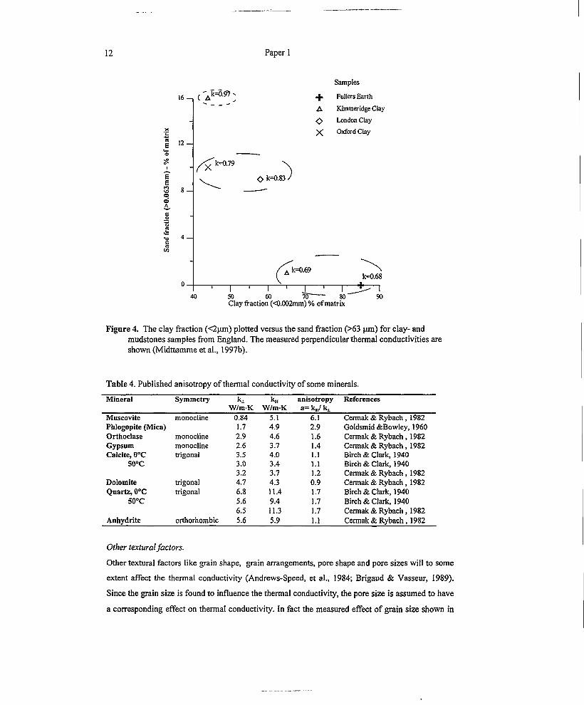
Grain size.
A correlation is observed between the grain size and the thermal conductivity (Rzhevsky & Norvik,
1971; Midttemme & Roaldset, 1997b; Midttemme et al, 1997b), with increasing thermal
conductivity with increasing grain sizes of the samples (Figure 3) and increasing sand content of
the clay samples (Figure 4). The grain size effect on thermal conductivity is logarithmic, with the
highest effect for the finest grained samples (Rzhevsky & Norvik, 1971; Midttemme & Roaldset
1997b). For unconsolidated samples the grain size fractions, in particular the sand fraction, were
found to have a strong effect on thermal conductivity, even greater than the complete mineralogy
(Midttemme et al., 1997c).
4.00-
3.00 —
zoo —
t i 11 mil
100 1000 Mean grain size (0,001mm)
Figure 3. Estimated matrix conductivity, by the geometric mean model, plotted against the mean grain size of artificial quartz samples. The solid line shows the logarithmic regression, R2= 0.86 (Midttemme & Roaldset, 1997b).
12 Paper 1
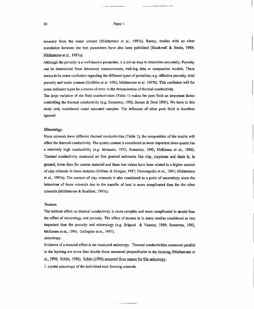
Samples
+ Fullers EarthA Kimmeridge Clayo London ClayX Oxford Clay
k=0.79
k=0.68
50 60 70 80Clay fraction (<0.002mm) % of matrix
Figure 4. The clay fraction (<2pm) plotted versus the sand fraction (>63 pm) for clay- andmudstones samples from England. The measured perpendicular thermal conductivities are shown (Midttemme et al., 1997b).
Table 4. Published anisotropy of thermal conductivity of some minerals.
Mineral Symmetry kiW/m-K
ki:W/m-K
anisotropy a= k„Z kx
References
Muscovite monocline 0.84 5.1 6.1 Cermak & Rybach , 1982Phlogopite (Mica) 1.7 4.9 2.9 Goldsmid &Bowley, 1960Orthoclase monocline 2.9 4.6 1.6 Cermak & Rybach, 1982Gypsum monocline 2.6 3.7 1.4 Cermak & Rybach, 1982Calcite, 0°C trigonal 3.5 4.0 1.1 Birch & Clark, 1940
50°C 3.0 3.4 1.1 Birch & Clark, 19403.2 3.7 1.2 Cermak & Rybach, 1982
Dolomite trigonal 4.7 4.3 0.9 Cermak & Rybach, 1982Quartz, 0°C trigonal 6.8 11.4 1.7 Birch & Clark, 1940
50°C 5.6 9.4 1.7 Birch & Clark, 19406.5 11.3 1.7 Cermak & Rybach, 1982
Anhydrite orthorhombic 5.6 5.9 1.1 Cermak & Rybach, 1982
Other textural factors.
Other textural factors like grain shape, grain arrangements, pore shape and pore sizes will to some
extent affect the thermal conductivity (Andrews-Speed, et al., 1984; Brigaud & Vasseur, 1989).
Since the grain size is found to influence the thermal conductivity, the pore size is assumed to have
a corresponding effect on thermal conductivity. In fact the measured effect of grain size shown in
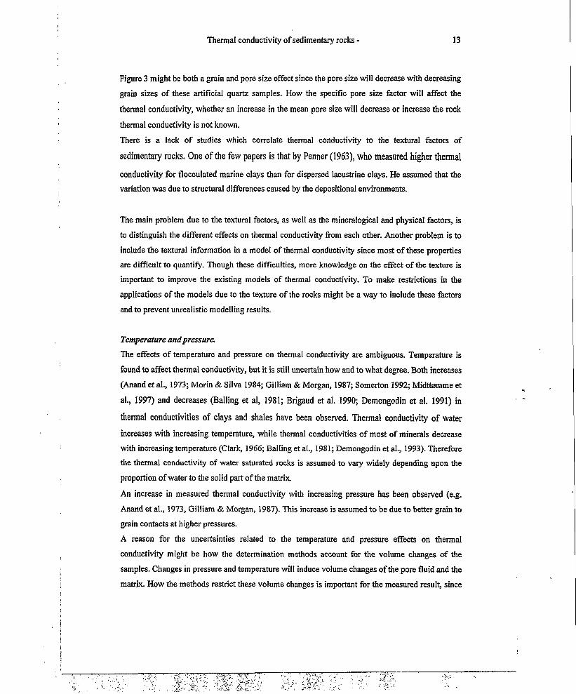
Thermal conductivity of sedimentary rocks - 13
Figure 3 might be both a grain and pore size effect since the pore size will decrease with decreasing
grain sizes of these artificial quartz samples. How the specific pore size factor will affect the
thermal conductivity, whether an increase in the mean pore size will decrease or increase the rock
thermal conductivity is not known.
There is a lack of studies which correlate thermal conductivity to the textural factors of
sedimentary rocks. One of the few papers is that by Penner (1963), who measured higher thermal
conductivity for flocculated marine clays than for dispersed lacustrine clays. He assumed that the
variation was due to structural differences caused by the depositional environments.
The main problem due to the textural factors, as well as the mineralogical and physical factors, is
to distinguish the different effects on thermal conductivity from each other. Another problem is to
include the textural information in a model of thermal conductivity since most of these properties
are difficult to quantify. Though these difficulties, more knowledge on the effect of the texture is
important to improve the existing models of thermal conductivity. To make restrictions in the
applications of the models due to the texture of the rocks might be a way to include these factors
and to prevent unrealistic modelling results.
Temperature and pressure.
The effects of temperature and pressure on thermal conductivity are ambiguous. Temperature is
found to affect thermal conductivity, but it is still uncertain how and to what degree. Both increases
(Anand et al., 1973; Morin & Silva 1984; Gilliam & Morgan, 1987; Somerton 1992; Midttemme et
al., 1997) and decreases (Balling et al, 1981; Brigaud et al. 1990; Demongodin et al. 1991) in
thermal conductivities of clays and shales have been observed. Thermal conductivity of water
increases with increasing temperature, while thermal conductivities of most of minerals decrease
with increasing temperature (Clark, 1966; Balling et al., 1981; Demongodin et al., 1993). Therefore
the thermal conductivity of water saturated rocks is assumed to vary widely depending upon the
proportion of water to the solid part of the matrix.
An increase in measured thermal conductivity with increasing pressure has been observed (e.g.
Anand et al., 1973, Gilliam & Morgan, 1987). This increase is assumed to be due to better grain to
grain contacts at higher pressures.
A reason for the uncertainties related to the temperature and pressure effects on thermal
conductivity might be how the determination methods account for the volume changes of the
samples. Changes in pressure and temperature will induce volume changes of the pore fluid and the
matrix. How the methods restrict these volume changes is important for the measured result, since

14 Paper 1
heat is mainly transferred by grain to grain contacts. A major problem with measurements at high
temperature or high pressure is drying of the samples.
Models.
Many models are developed to estimate thermal conductivities from other known parameters.
However, no universal model for the thermal conductivity of sedimentary rock has yet been found.
The models can be grouped in three types (Somerton, 1992).
1. Mixing law models.
2. Empirical models.
3. Theoretical models.
Mixing law models combine values of the thermal conductivity of the rock matrix (ks) with the
conductivity of the pore fluid (kj) on the basis of porosity. These models are of a general character
and might be used for all sediment types. Thermal conductivity is in empirical models related to
measured physical parameters, log data and to laboratory data. These methods have their
shortcomings in that the resulting models may be applicable only to a particular suite of rocks
being investigated (Somerton, 1992). Theoretical models are based on heat transfer theory for
simplified geometries. The difficulty with these models is the degree of simplification necessary to
obtain a solution. There is still a lack of detailed knowledge on how the heat is transferred through
sedimentary rocks, in particular what happens in the transitional phase between grain-pore and
grain-grain. Preferably, one would use a theoretical model to describe the physics of heat
conduction, but sufficiently reliable models have not yet been developed, and empirical
modifications of the equations are needed (Zimmerman, 1989; Somerton, 1992).
The mixing law models have dominated in the recent thermal conductivity studies. The three basic
mixing law models are the arithmetic mean (Equation 3), geometric mean (Equation 2) and the
harmonic mean (Equation 4).
k = tjkj + (1 - $)&, eq. 3
1 ± (1-fl eq.4
The harmonic and arithmetic mean models are based on parallel and series arrangement of the
components relative to the direction of heat flow (Figure 5). These two models are used, among
others, by Vacquier et al. (1988), Somerton (1992), Pribnow & Umsonst (1993) and McKenna et
al. (1996). The values estimated by these models are assumed to give the upper (&ma%) and lower

Thermal conductivity of sedimentary rocks 15
bound of thermal conductivity for a rock of given composition (Woodside & Messmer, 1961;
Zimmerman, 1989 Schon, 1996). The geometric mean model gives a mean value of the arithmetic
1 2Heat flow Heat flow
HUH HHtl
mm P
P
Figure 5. Sheet models of the two mixing law models. 1) arithmetic mean model,2) harmonic mean model, kharm=kll m- matrix, p- pore fluid (Schon, 1996).
and harmonic means. This model is the most widely used model by among others, Woodside &
Messmer (1961), Sass et al. (1971), Balling et al. (1981), Brigaud et al. (1990), Demongodin et al.
(1991), McKenna et al. (1996) and Midttomme et al. (1997c).
I
8
2.00 ■
1.60-
120 -
•5 0.80 •
0.40 —
0.00-
Samples0 Siltstone from Heather Formation
-J- Oxford Clay
+ London Clay
Fullers Earth
KimmeridgeClay
0.00 0.20 0.40 0.60Water content (0.00 -1.00)
0.80l
1.00
Figure 6. Thermal conductivity estimated by the arithmetic, geometric and harmonic mean model plotted versus water content, kj— 0.60 W/m-K, £,=1.50 W/m-K. Parallel and perpendicular measured thermal conductivities of 5 samples are shown.

16 Paper 1
The main criticism of the geometric mean model is that it does not take account for the texture of
the samples, and therefore is valid only for isotropic rocks (Brigaud & Vasseur, 1989; Somerton,
1992). The harmonic, arithmetic and geometric mean models are plotted as a function of the water
content, together with 5 measurements of parallel and perpendicular thermal conductivities (Figure
6). Even for these claystones and siltstones the measured anisotropies are, except for Fullers Earth,
higher than the theoretically maximum values based on arithmetic and harmonic means (amax=
karim/kharm)• An explanation for this underestimate is that the arithmetic and harmonic mean
models only take account of the structural arrangement of the pores and the matrix within the rocks
and not to the crystal anisotropy of the individual rock forming minerals (Table 4), which are most
important for the anisotropy effect of clay and mudstones (Demongodin et al., 1993). To take
account of this crystal anisotropy effect, a higher parallel matrix conductivity (ksii) than
perpendicular matrix conductivity (kSi) has to be used. By using the arithmetic and harmonic mean
models, the estimated anisotropy depends on the value of matrix conductivity (ks) (Figure 7). A
low matrix conductivity gives low values of thermal conductivity. The opposite is often measured,
where shales and claystones with low matrix conductivity have highest anisotropies. The most
important anisotropic effect of thermal conductivity is not taken account of by using the arithmetic
and harmonic mean models. From this assumption of the anisotropy, we prefer the geometric mean
model, used with a higher matrix conductivity parallel than perpendicular to the layering to account
for the thermal conductivity anisotropy.
The uncertainty related to the choice among the three mixing law models depends on the ratio k/kf
and porosity. For water saturated samples, where the fluid conductivity is assumed constant, the
AyXyratio is determined by the matrix conductivity. According to Woodside & Messmer (1961),
Lovell (1985) and Ungere et al. (1990), the geometric mean is valid only if the k/kf ratio is not too
large. For ratios greater than 20 the geometric mean model tends to substantially overestimate the
measured values. The model was for this reason proven correct for clays with low matrix
conductivity (Morin & Silvia, 1984). Thermal conductivities are plotted with the arithmetic,
geometric and harmonic mean models as a function of the porosity in Figure 7. Thermal
conductivity of the fluid is set equal to water conductivity (Ay=0.60 W/m-K) and the matrix
conductivity (ks) is constant equal a) 1.0 W/m-K, b) 2.5 W/m-K or c) 5.0 W/m-K. The deviation
between the geometric mean model and the two other mixing law models is shown for porosities of
10%, 20%, 40% and 60% respectively. This discrepancy in estimated thermal conductivity varies
from 1% to 68%. The highest sensitivity of the choice of mixing law models is for the highest
matrix conductivity in the porosity range of 40-60 %.

0.90 -
Porosity (water content) %
b) “0
ZOO -
1.00 -
Porosity (water content) %
Porosity (water content) %
Figure 7. Thermal conductivity estimated by the arithmetic, geometric and harmonic mean model plotted versus porosity where k/= 0.60 W/m-K, and ks = a) 1.0 W/m-K, b) 2.5 W/m-K, and c) 5.0 W/m-K. The discrepancies between the geometric mean model and the two other mixing law models for porosities of 10 %, 20%, 40% and 60% are shown.

18 Paper 1
The matrix conductivity (ks) is a point of uncertainty in mixing law models. This parameter has to
take account of the mineralogical and textural effects on the thermal conductivity. Different values
and models of matrix conductivity (ks) have been used. In the simplest geometric mean models
matrix conductivity is set as constant (Table 5), while matrix conductivity in complex models is
estimated from the mineralogy (e.g. Brigaud & Vasseur, 1989; McKenna et al., 1996) and by use of
mineralogy and grain size fraction (Midttomme et al., 1997c) (Table 6).
Table 5. Thermal conductivities used in the geometric mean equation.
SampleMatrix
conductivity(ks)
W/m-K
Waterconductivity
(kj)W/m-K
References
Shale 2.35 0.60 Sekiguchi, 19841.9 Grigo et al., 1993
Sandy shale 2.1 Grigoetal.,1993Clay, claystone, shale 3.43 0.46 Balling et al., 1981Clay 1.2-1.4 0.60 Demongodin et al.,1991
1.1 Grigo et al., 1993Claystone 1.5-3 0.56 Chapman et al., 1984Siltstone 3.2 Grigo et al., 1993Mudstone,siltstone 2.5 0.61 Bloomer, 1981Sandy siltstone 2.49 0.60 Sekiguchi, 1984Sandy mudstone 3.0 0.61 Bloomer, 1981Shaly sandstone 2.66 0.60 Sekiguchi, 1984Muddy sandstone 3.2 0.61 Bloomer, 1981Sandstone 4.88 0.69 Balling et al., 1981
6.60 0.60 Demongodin et al.,19915-7 0.56 Chapman et al., 19843.4 Grigo et al., 1993
Quartzose sandstone 7.96 0.60 Sekiguchi, 1984Quartz sandstone 3.7 0.61 Bloomer, 1981Carbonate 3.24 0.54 Balling et al., 1981
3.0 0.59 Matsuda & Herzen, 1986Limestone 3.2 0.61 Bloomer, 1981
3.2 0.60 Demongodin et al.,19913.6 Grigo et al., 1993
167 wells North Sea 0.8-8.3 0.60 Andrews-Speed et al.,1984Gulf of Mexico 2.02 0.63 Sharp & Domenico, 1976Sedimentary rock 2.51 0.58 Smith & Chapman, 1983
1.7-4.2 0.4 Lerche, 1993
The accuracy of the estimate of the matrix conductivity depends on the rock information available. Of even greater importance is the right choice of model. Disagreements between estimated and measured thermal conductivities are shown for clay- and mudstones (Figure 8) and unconsolidated sediments (Figure 9). The thermal conductivities in these studies were estimated by the geometric
mean model, where matrix conductivities were estimated from the mineralogy (Table 6). From the
assumptions that the measurements in these studies are correct, the model fails to predict the
thermal conductivity for these samples. Somerton (1992) assumed a basic difference in the thermal

Thermal conductivity of sedimentary rocks - 19
Table 6 Advanced models of matrix conductivity from mineral and grain size conductivities.
Samples
Horai(1971)
Pulverizedsamples
Brigaud & Vasseur (1989)
Sandstones and artificially recompacted clay samples
Midttemme et al., (1997a)
Argillaceous sediments from
North Sea
Midttemme et al., (1997c)
Unconsolidated sediments from Voting Basin
R2=0.864 R^O.882
k, 0.60 0.60 0.60 0.60Quartz 7.8 7.70 + 0.88 1.01 5.03 6.82Feldspar 2.3 1.02 2.97 3.49Calcite 3.4 3.26 + 0.23 1.68 3.62Dolomite 5.1 5.33+0.26 1.64Pyrite 19.2 1.41
k, Kaolinite 2.8 2.64 + 0.20 0.91 0.08 2.80Chlorite 5.1 3.26 ±0.25Smectite 1.88 ±0.13 1.42 3.34 1.61Elite 1.8 1.85 ±0.23 1.42 3.34 1.61>63 pm 5.792pm-63pm 1.52<2pm 1.89
Samples0 London Clay
+ Fullers Earth
A KimmeridgsClay
X Oxford Clay
Estimated thermal conductivity - W/mK
Figure 8. Estimated thermal conductivity versus measured thermal conductivity for clay and mudstones from England. The solid line is the unity line (1:1). The dotted line is the regression line (Midttemme et al., 1997b).

20 Paper 1
1.60-
1.20
080 _
30 1.20 1jEstimated thermal conductivity - W/mK
Figure 9. Estimated thermal conductivity versus measured thermal conductivity for unconsolidated sediments from Voring Basin. The solid line is the unity line (1:1) The dotted line is the regression line (Midttomme etal., 1997c).
characteristic of consolidated rocks and unconsolidated sand. He therefore considered modelling
the two systems separately. Midttomme et al. (1997a) assumed that quartz grains isolated in a clay
matrix contribute less to the rock conductivity than quartz grains in contact with another. A
distinction between matrix supported and grain supported sediments in modelling of the thermal
conductivity was suggested by Eirik Vik (pers. comm., 1997). Because of differences in heat
transferred through sedimentary rocks, no universal model of thermal conductivities exists today.
All models are to some degree restricted either to specific rock types, in variation of ranges of the
parameters or location. The restrictions in the mixing law models are caused by the estimation of
matrix conductivity. According to Andrews-Speed et al. (1984), the matrix conductivity varies by
one order of magnitude from 0.8 to 8.3 W/m K (Table 5). To model these variations we suggest the
development of specific matrix conductivity models for the different types of matrix. For some
types of sediments a constant matrix conductivity might save the purpose. For other sediments
types the mineralogy, depositional environment, grain size distribution etc., seems to affect the
matrix conductivity and might be taken into account in the thermal conductivity model.

Thermal conductivity of sedimentary rocks - 21
CONCLUSION.
Temperature cannot be predicted accurately in sedimentary basins, without knowledge of the
thermal conductivities of the sedimentary sequences. There are still uncertainties related to the
determination of thermal conductivities. Discrepancies in the thermal conductivity measurements
are observed. This warrants more basic studies; i.e. validity of the method of measurements due to
sediment type. A standardisation of the procedures of sample preparation and experimental
conditions is needed to prevent unrealistic measurements.
No universal model of thermal conductivity exists today, and it will be difficult to develop such a
model since the different sediment types seem to have basic differences in the heat transfer.
Models based on the geometric mean model seem to be bestl so far. The effect of porosity on
thermal conductivity can be taken into account by this model. The matrix conductivity (ks) in the
model depends on the mineralogy and texture of the sedimentary rocks. Our experience with clays
and mudstones shows that the textural influence on thermal conductivity is underestimated by
many of the existing models. How the different mineralogical and textural factors will affect
thermal conductivity depends on the sediment types, lithology and texture. To define the range of
application for the models due to type and texture of sediment is important to obtain realistic
estimates applicable in basin modelling.
REFERENCES.
Anand, J., Somerton, W.H. & Gomaa, E. 1973. Predicting thermal conductivities of formations from other known properties. Society of Petroleum Engineers Journal. 267-273.
Andrews-Speed, C.P., Oxburgh, E.R. & Cooper, B.A. 1984. Temperatures and depth-dependent heat flow in western North Sea. AAPG Bulletin, 68, 1764-1781.
Balling, N., Kristiansen, J.I., Breiner, N., Poulsen, K.D., Rasmussen, R. & Saxov, S. 1981. Geothermal measurements and subsurface temperature modelling in Denmark. Geoskrifter, 16, Department of Geology, Aarhus University.
Beck, A.E, 1988. Methods for determining thermal conductivity and thermal diffusivity. In Haenel, R., Rybach, L. & Stegena, L. (eds) Handbook of Terrestrial Heat Flow Density Determination: Dordrecht, Kluwer, 87-124.
Benfield, A.E. 1947. A heat flow value for a well in California. American Journal of Science, 245,1-18.
Birch, F. 1954. Thermal conductivity, climatic variation and heat flow near Calumet, Michigan. American Journal of Science, 252, 1-25.
Birch, F. & Clark, H. 1940. The thermal conductivity of rocks. American Journal of Science, 238,529-558.

22 Paper 1
Blackwell, D. D. & Steele, J. L. 1989. Thermal conductivity of sedimentary rocks: measurements and significance. In: Naeser, N. D. & McCulloh, T. H. (eds) Thermal History of Sedimentary Basins, Methods and Case Histories. Springer Verlag, New York, 13-36.
Bloomer, J.R. 1981. Thermal conductivities of mudrocks in the United Kingdom. Quarterly Journal of Engineering Geology, 14,357-362.
Brigand, F. & Vasseur, G. 1989, Mineralogy, porosity and fluid control on thermal conductivity of sedimentary rocks. Geophysical Journal, 98, 525-542.
Brigaud, F., Chapman, D.S. & Le Douaran, S. 1990. Estimating thermal conductivity in sedimentary basins using lithological data and geophysical well logs. AAPG Bulletin, 74, 1459-1477.
Bullard & Niblett, 1951. Mon. Not. Roy. Astr. Soc., Geophys. Suppl. 6,222, (cited from Clark, 1966).
Chapman, D.S., Keho, T.H., Bauer, M.S. & Picard, M.D. 1984. Heat flow in the Uinta Basin determined from bottom hole temperature (BHT) data. Geophysics, 49,453-466.
Cermak, V. & Rybach, L. 1982. Thermal properties. In Hellwege, K.-H. (ed) Landolt-Bornstein Numerical Data and Functional Relationships in Science and Technology, New Series, Group V. Geophysics and Space Research,. 1, Springer-Verlag, Berlin.
Clark, S.P. jr. 1966. Handbook of physical constants. The Geological Society of America, Inc. Memoir 97.
Demongodin, L., Pinoteau, B., Vasseur, G. & Gable, R. 1991. Thermal conductivity and well logs: a case study in the Paris Basin. Geophysical Journal International, 105, 675-691.
Demongodin, L., Vasseur G. & Brigaud, F. 1993. Anisotropy of thermal conductivity in clayey formations. In Dore, A.G., Auguston, J.H., Hermanrud, C., Stewart, D.S. & Sylta, 0. (eds) Basin modelling: advances and applications, Norwegian Petroleum Society (NPF) Special Publication 3, Elsevier, Amsterdam, 209-217.
Dortman, N.B. 1976. Fiziceskie svoistva gornich porod ipolesnich iskopamych. Izdat. Nedra Moskva (cited from Schon, 1996).
Farouki, O.T. 1981. Thermal properties of soils. CRREL Monograph 81-1.
Fjeldskaar, W., Mykkeltveit, J., Christie, O.H.J., Johansen, H., Langfeldt, M., Tyvand, P., Skurve, O. & Bjerkum, P.A. 1990. Interactive 2D Basin Modelling on Workstations. Proc. SPE 20350 Petroleum Computer Conferance. Denver, Colorado, 181-196.
Gallagher, K., Ramsdale, M., Lonergan, L. & Morrow, D. 1997. The role of thermal conductivity measurements in modelling thermal histories in sedimentary basins. Marine and Petroleum Geology, 14, 201-214.
Gilliam, T.M. & Morgan, I.L. 1987. Shale: measurement of thermal properties. Oak Ridge National Laboratory ORNL /TM-10499, Oak Ridge, Tennessee.
Griffiths, C.M., Brereton , N.R, Beausillon R. & Castillo, D. 1992. Thermal conductivity prediction from petrophysical data: a case study. In Hurst, A., Griffiths, C.M. & Worthington, P.F. (eds) Geological Applications of Wireline Logs II, Geological Society Special Publication, 65,299-315.
Goldsmid, H.J. & Bowley, A.E. 1960. Thermal conduction in mica along the planes of cleavage, Nature, 187, 864-865.
Grigo, D., Maragna, B., Arienti, M.T., Fiorani, M., Parisi, A., Marrone, M., Sguazzero, P. & Uberg, A.S. 1993. Issues in 3D sedimentary basin modelling and application to Haltenbanken, offshore Norway. In Dore,

Thermal conductivity of sedimentary rocks - 23
A.G., Auguston, J.H., Hermanrud, C., Stewart, D.S. & Sylta, 0 (eds) Basin modelling: advances and applications, Norwegian Petroleum Society (NPF) Special Publication 3, Elsevier, Amsterdam, 455-468.
Horai, K.I. 1971, Thermal conductivity of rock-forming minerals. Journal of Geophysical Research. 76, 1278-1308.
Jensen, R.P. & Dore, A.G. 1993. A recent Norwegian Shelf heating event - fact or fantasy ? In Dore, A.G., Auguston, J.H., Hermanrud, C., Stewart D.S. & Sylta, 0. (eds) Basin modelling: advances and application. Norwegian Petroleum Society (NPF) Special Publication 3, Elsevier, Amsterdam, 85-106.
Jessop, A.M. 1990. Thermal Geophysics. Elsevier.
Johansen, 0. 1975. Varmeledningevne av jordarter. Dr.ing avhandling, institutt for kjoleteknikk, Norwegian Institute of Technology (NTH), Trondheim. (Thermal conductivity of soils. Ph.D. thesis, Cold Region Research and Engineering Laboratory (CRREL) Draft Translation 637, 1977, ADA 044002,Hanover, New Hampshire.
Kappelmeyer, O. & Haenel, R. 1974. Geothermics with special reference to application. Geopublication associates. Geoexploration Monographs. Series 1 - No.4 Gebruder Bomtraeger, Berlin, Stuttgart
Kobranova, V.N. 1989. Petrophysics, Mir Publisher, Moscow, Springer-Verlag Berlin. (Cited from SchSn, 1996)
Lerche, I. 1993. Theoretical aspects of problems in basin modelling. In Dore, A.G., Auguston, J.H., Hermanrud, C., Stewart D.S. & Sylta, 0. (eds) Basin modelling: advances and application. Norwegian Petroleum Society (NPF) Special Publication 3, Elsevier, Amsterdam, 35-65.
Lovell, M.A. 1985. Thermal conductivities of marine sediments, Ouarterly Journal of Engineering Geology, 18, 437-441.
Matsuda, J.-I. & Von Herzen, R.P. 1986. Thermal conductivity variation in a deep-sea sediment core and its relation to H20, Ca and Si content Deep-Sea Research, 33,165-175.
McKenna, T. E., Sharp, J. M. Jr., & Lynch, F.L. 1996. Thermal conductivity of Wilcox and Frio sandstones in south Texas (Gulf of Mexico Basin). AAPG Bulletin, 80,1203-1215.
Middleton, M. 1994. Determination of matrix thermal conductivity from dry drill cuttings. AAPG Bulletin, 78,1790-1799.
Midttomme, K., Roaldset E. and Brant)es, J.G. 1996. Thermal conductivity of alluvial sediments from the Ness Formation, Oseberg Area, North Sea. EAEG 58th Conference, Extended Abstracts Volume 2, P552, Amsterdam.
Midttomme, K. & Roaldset E. 1997a. The influence of clay minerals on thermal conductivity of sedimentary rocks. Nordiska fdreningen for lerforskning, Meddelande nr 11.
Midttomme, K. & Roaldset E. 1997b. The effect of grain size on thermal conductivity of quartz sands and silts. Petroleum Geoscience. In press.
Midttomme, K., Roaldset E. & Aagaard, P. 1997a, Thermal conductivity of argillaceous sediments. In. McCann, D.M., Eddleston, M., Penning, P.J & Reeves, G.M. (eds) Modern Geophysics in Engineering Geology, Geological Society Engineering Special Publication, 12,355-363.
Midttomme, K., Roaldset E. & Aagaard, P. 1997b. Thermal conductivity of selected clay- and mudstones from England, Clay Minerals, 33,131-145.
24 Paper 1
Midttemme, K., Saettem, J. & Roaldset, E. 1997c. Thermal conductivity of unconsolidated marine sediments from Voting Basin, Norwegian Sea. In: Middleton, M.F. (ed.) Nordic Petroleum Technology Series: Two, Nordisk energiforskningssamarbejde. In press.
Morin, R. & Silva, A.J. 1984. The effects of high pressure and high temperature on some physical properties of ocean sediments, Journal of Geophysical Research, 89-B1, 511-526.
Mossop & Gainer, 1951. Jour. Chem. Met., Min. Soc., S. Afr. 52, 61, (cited from Clark, 1966).
Penner, E. 1963. Anisotropic thermal conduction in clay sediments. Proceedings, International Clay Conference, Stockholm, Pergamon Press, Elmsford, 1,365-376.
Pribnow, D. & Umsonst, T. 1993. Estimation of thermal conductivity from the mineral composition: Influence of fabric and anisotropy. Geophysical Research letters, 20, 2199-2202.
Rzhevsky, V. & Novik, G. 1971. The Physics of Rocks. Mir Publishers, Moscow, (translated from the Russian by Chatterjee, A. K).
Sass, J.H., Lachenbruch, A.H. & Munroe, R.J. 1971. Thermal conductivity of rocks from measurements on fragments and its application to heat-flow determinations. Journal of Geophysical Research, 76,3391-3401.
Schon. J.H. 1996 Physical properties of rocks: fundamentals and principles of petrophysic. Seismic exploration, vol. 18, Elsevier Science ltd, Oxford.
Sekiguchi, K. 1984. A method for determining terrestrial heat flow in oil basinal areas. Tectonophysics,103, 67-79.
Sharp, J.M. jr. & Domenico, P.A. 1976. Energy transport in thick sequences of compacting sediment. Geological Society of American Bulletin, 87, 390-400.
Slusarchuk, W.A. & Foulger, P.H. 1973. Develoment and calibration of a thermal conductivity probe apparatus for use in the field and laboratory, National Research Council of Canada, Div. of Building Research, Technical Paper, 388.
Smith, L. & Chapman, D.S. 1983. On the thermal effects of groundwater flow.l. Regional scale systems. Journal of Geophysical Research, 88, Bl, 593-608.
Somerton, W.H. 1992. Thermal properties and temperature related behavior of rock/fluid systems. Developements in Petroleum Sciences, 37, Elsevier, Amsterdam.
Ungerer, P., Burrus, J., Doligez, B., Chenet, P.Y. & Bessis, F. 1990. Basin evaluation by integrated two- dimensional modeling of heat transfer, fluid flow, hydrocarbon generation and migration. AAPG Bulletin, 74, 309-335.
Vacquier, V., Mathieu, Y., Legendre, E. & Blondin, E. 1988. Experiment on estimating thermal conductivity of sedimentary rocks from oil well logging. AAPG Bulletin, 72, 758-764.
Von Herzen, R.P. & Maxwell, A.E. 1959. The measurement of thermal conductivity of deep sea sediments by a needle-probe method. Journal of Geophysical Research, 64, 1557-1563.
Woodside, W. & Messmer, J.H. 1961. Thermal conductivity of porous media. Journal of Applied Physics, 32, 1688-1706.
Zimmerman, R. W. 1989. Thermal conductivity of fluid-saturated rocks. Journal of Petroleum Science and Engineering,3, 219-227.

Paper 2

Thermal conductivities of argillaceous sediments
K. Midttemme1, E. Roaldset1 & P. Aagaard2
1 Department of Geology and Mineral Resources Engineering, Norwegian University of Science and Technology, 7034 Trondheim, Norway^ Department of Geology, University of Oslo, P.O. Box 1047, Blindem, 0315 Oslo, Norway
Abstract: Thermal conductivities of selected samples of shales, clay- and mudstones from the Norwegian Continental Shelf have been measured with a divided bar apparatus. The samples investigated are from conventional cores and side wall cores. Thermal conductivities for water- saturated samples measured perpendicular to the layering vary from 0.79 to 1.14W/m K. The conductivities measured parallel to the layering are up to 1.7 times higher than those measured in the perpendicular direction. The investigation also confirms that the temperature has an influence on the conductivity. A model to predict thermal conductivity, based on water content and mineralogy has been proposed and tested.
Thermal conductivity of sediments is a key parameter in many studies of sedimentary basins because it controls the conductive heat flow, and therefore also the temperature distribution in sediment successions. Great efforts have been made to determine.sediment conductivity both from laboratory measurements and from calculations from other known parameters. Still, there is lack of knowledge about the thermal conductivity of sedimentary rocks, and in particular little available information exists on the influence of clay minerals (Brigand & Vasseur 1989).
The variation of the thermal conductivities of sediments is found to depend mainly on mineralogy, porosity and texture (Woodside & Messmer 1961; Anand et al. 1973; Johansen 1975; Farouki 1981; Brigaud & Vasseur 1989). Temperature will also have an influence on the conductivity (Anand et al. 1973; Gilliam & Morgan 1987; Blackwell & Steele 1989; Demongodin et al. 1993).
Factors influencing the thermal conductivity
MineralogyMineralogy is the most important factor controlling thermal conductivities of sedimentary rocks. Thermal conductivities of selected rock forming minerals from Brigaud & Vasseur (1989) are shown in Table 1. These results are comparable with measurements by Horai (1971) and values applied in the basin modelling system (BMT) developed at Rogaland Research (Fjeldskaar et al. 1990).
Rocks with greater proportions of the clay minerals smectite, illite and mixed layer illite/smectite will have lower conductivities than rocks with the same proportion
of other minerals specially quartz and pyrite. The low conductivities of smectite and illite have been explained by the layering of the minerals (Blackwell & Steele 1989; Demongodin et al. 1993) although kaolinite and chlorite have the same layered structure but do not have such low thermal conductivities. The various clay minerals affect pore spaces in different ways, whether they are laminated, dispersed, in pore lining or in pore bridging. These structural differences may explain the differences in conductivity between the clay minerals.
Water content (porosity)Thermal conductivity of water is 0.60 W/m K at 20°C and lower than the conductivity of the minerals. Thus, a decrease in water content would lead to an increase in the thermal conductivity of sediments. Because of the smaller
Table 1. Conductivity of rode forming minerals (Brigaud & Vasseur 1989)
Mineral K(W/mK)
Quartz 7.7Feldspar 2.3Pyrite* 19.2Calcite 3.3Dolomite 5.3Anhydrite 6.3Chlorite 3.3Kaolinite 2.6Smectite 1.9Illite 1.8Illite/smectite 1.8
•Horai (1971)
From McCann, D. M., Penning, P. J. & Reeves, G. M. (eds), 1997, Modem Geophysics in Engineering Geology. Geological Society Engineering Geology Special Publication No. 12, pp. 357-365.

358 K. MIDTT0MME ET AL.
difference between thermal conductivity of water and clay minerals, the effect of water content is less for low conductive materials such as shales and claystones, than for high conductive sediments as quartz rich sandstones.
Porosity is a more common used factor instead of water content when considering percentage of water in water saturated samples. Porosity is the volume of the pores in the material while water content includes all water in the material, also bound and constitutional water.
Texture
Sedimentary rocks are inhomogenous and anisotropic. The thermal conductivity will vary on micro scale within the single sediment layer, and also, with orientation to the layering. The difference in the conductivities measured parallel to and perpendicular to the layering, the anisotropy effect, is found to be considerable (Gilliam & Morgan 1987; Prestholm & Fjeldskaar 1993). Variation
x
Fig. 1. Location of the three wells on the Norwegian Continental Shelf.

THERMAL CONDUCTIVITIES OF ARGILLACEOUS SEDIMENTS 359
in conductivity caused by the texture can be divided into effects of crystal orientation for a given mineral and effects of small-scale heterogenities within a given lithology (Demongodin et al. 1993).
Temperature
Variation in temperature will induces changes in bulk conductivity. (Anand et al. 1973; Balling et al. 1981; Demongodin et al. 1993). The actual temperatures in the economic zones of sedimentary basins range from 0°C to about 200°C. Somerton (1992) reported moderate negative gradients of thermal conductivity with temperature for high conductive rocks whereas small positive gradients for low conductivity rocks. Gilliam & Morgan (1987) measurements on shales show a slight increase in thermal conductivity with increasing temperature up to about 90°C. Both studies were based on experimental data from laboratory measurements. The effect of temperature of in situ conditions of the material may be more complex because the temperature also will influence other chemical and physical factors which may effect thermal conductivity. There is assumed to be two processes which will occur and effect thermal conductivity when increasing the temperature: the activity of molecules and atoms will increase and increase the thermal conductivity and to some extent there will be drying of the samples with increasing temperature which will decrease the conductivity.
Theoretical modelling of thermal conductivity
Various models have been proposed for estimating the thermal conductivity of sedimentary rocks. One of them, the geometrical mean model, has been shown to predict satisfactorily the conductivity, at least when anisotropy effects can be neglected (Woodside & Messmer 1961; Johansen 1975; Brigand & Vasseur 1989; Demongodin et al. 1991). The geometric mean is a simple model which only takes account of the thermal conductivity of the matrix, k„ thermal conductivity of the water, km and water content, w. The bulk thermal conductivity of a water saturated rock is k given by Equation (1):
k = kl-k[x-v) (1)
where k„ is 0.6W/mK.
Material investigated
20 mudstone samples from three wells (A, B and C) on the Norwegian Continental Shelf were investigated (Fig. 1).
Samples from well A are of Tertiary mudstones. The well is situated on the northwestern flank of the Utsira
High in the North Sea. The samples were prepared from side wall cores. The sampling interval is 1200-2500m(RKB). Mineralogical, petrological and petrophysical investigations of the samples are reported by Tyridal (1994). The material consists of sandy mudstones where fragments of light claystones and grains of quartzite are randomly distributed in a darker clayey grey matrix. The fragmental character of the sediments is probably a result of mass flow caused by a turbidity current. Smectitic illite/smectite mixed layer minerals are found to be the dom-inating mineral. No laminations are visible. The side wall cores were contaminated with drilling fluids, and barite from the drilling fluids complicated the mineral identification by X-ray diffractograms.
Samples from well B are cut from conventional core samples from the Upper Jurassic Heather Formation. The well is located on the western flank of the Horda Platform. The sampling interval is 2125-2169 m(RXB) and the water depth is 147 m. The samples have been investigated by Zhang et al. (1992) and Roaldset & Gjelsvik (1993). The Heather Formation samples represent moderately to poorly sorted micaceous sandy siltstone. The material has a poorly developed lamination modified by bioturba- tion. The main constituents are quartz, feldspar and mica in a clayey matrix.
Well C is drilled on Haltenbanken off Mid-Norway. The two samples investigated from this well were cut from a conventional core from the Upper Cretaceous succession at a depth of 2437 m(RKB). The samples are fissile mudstones with a clay mineral content of 30% and a quartz content of 42%.
Laboratory measurementsThermal conductivities were measured with a divided bar apparatus developed at Department of Refrigeration Engineering, Norwegian University of Science and Technology, and described by Brendeng & Frivik (1974) (Fig. 2). As the equipment originally was designed for larger samples a slightly modified method was applied were the samples were measured against a reference sample.
The samples were measured in water saturated state. To reduce the effect of water movement, the temperature gradient across the samples was minimalized to 1.0-3.5 K. The sizes of the samples were cores with radius 2.5 cm and length 3.0 cm for A and cubes with sides 3.0 cm for B and C samples.
To test the influence of the temperature on the conductivity the samples were measured at different mean temperatures. All samples were tested at two or three different mean temperatures between 10-60°C.
The mineralogy was determined by standard X-ray diffraction techniques described among others of Brindley & Brown (1980) and Moore & Reynolds (1989). The

360 K. MIDTT0MME ET AL.
HOT PLATE
THERMOCOUPLEiSEDIMENTi
COLD PLATE
INSULATION
Fig. 2. A section through the divided bar apparatus.
Water content was calculated from measurements of bulk and grain densities (Equation 2).
w = 1 — — (2)Pd
where w is the water content (volume of water of total volume), pm is the bulk density (g/cm3) and pj is the grain density (g/cm3).
The densities were measured with pycnometer and calculated from the measured weight and volume of the samples. The samples were dried at 105°C before grain density was determined. Water content calculated in volume of water of total volume of material is often considered equal to porosity.
diffractograms were interpreted manually by calculating the areas of the characteristic peaks of the untreated diffractograms. The peak areas were corrected by means of ‘weighting factors’ developed by H.G.Rueslatten and generally applied at the X-ray Diffraction Laboratory at the Department of Geology and Mineral Resources Engineering, Norwegian University of Science and Technology. The quantification is considered to be semi-quantitative with an average error in the order of 5-10% (Rundberg 1991).
Results and discussionThe results of the measurements of water content, mineralogy and thermal conductivities are presented in Table 2.
The measured thermal conductivities vary in the range of 0.71-1.14W/mK. The measured conductivities are similar to those reported by Gilliam & Morgan (1987) on shales from Green River Formation, USA, who also used a divided bar apparatus. However, the values of
Table 2. Results of thermal measurements together with water conent, quartz and clay mineral contents
Sample DepthmRKB
Watercontent
Content of clay minerals
Quartzcontent[%]
Thermalconductivityperpendicular*k,(W/mK)
Thermalconductivityparallel1kn(W/mK)
Anisotropyeffectkn/ki
Central A1 1265 42 34 36 1.06North Sea A2 1330 40 45 33 0.87
A3 1450 33 39 26 0.85A4 1510 38 35 30 0.85A5 1610 40 27 45 0.83A6 1675 40 38 26 0.82A7 1765 33 23 35 0.79AS 1835 38 27 38 0.83A9 1874 36 16 42 1.14A10 2033 24 42 26 0.96All 2450 21 42 37 1.08A12 2576 9 26 50 0.86
Northern B1 2125 13 50 21 0.97 1.65 1.70North Sea B2 2125 13 50 21 0.93
B3 2131 19 51 21 0.71 1.15 1.62B4 2155 11 58 18 0.97B5 2161 15 70 13 1.20B6 2169 17 54 19 1.02 1.54 1.51
Mid-Norwegian Cl 2437 21 30 42 0.92f 1.08$ 1.17Shelf C2 2437 21 30 42 1.04f 1.17$ 1.13
* Measured at temperature between 22—38°C. t Measured 55° to the layering, j Measured 35° to the layering.

THERMAL CONDUCTIVITIES OF ARGILLACEOUS SEDIMENTS 361
this work are significantly lower than measurements on argillaceous sediments previous reported (Bloomer 1981; Brigaud & Vasseur 1989; Demongodin et al. 1993; Fjeldskaar et al. 1993). In their studies the conductivities were measured with the needle probe technique, which is considered as an easier, but not so exact, method for determination of thermal conductivities. The divided bar apparatus is considered more appropriate for measuring conductivity of anisotropic material than the needle probe technique.
The measured sample conductivity varied slightly with the test temperature. In tested temperature range of +10—h60°C the conductivity varied from —0.016 to +0.013W/mK for increase of 10K.
The low value of 0.71 W/mK of sample B3 differs from the other measured values. This value is probably due to drying of the material and is therefore omitted in the further discussion.
The effect of factors influencing the thermal conductivity
Water contentThe measured thermal conductivities perpendicular to the layering are plotted against the water content in Fig. 3.
CeoMttic asaa aodsl
- • k(j) ■ 6.1« ' k(e) * 1.0
1.20 -i
i 1.00 -
0.80-
Water content - % of voltae
Fig. 3. Influence of water content on thermal conductivity. Geometric mean model (Eq. I) calculated with thermal conductivity of water equal 0.6 W/mK and thermal conductivity of matrix, kly equal to 0.8, 1.0 and 1.2 W/mK are also plotted.
The trend is a decrease in thermal conductivity with increasing water content. This agrees with the geometric mean model. The relationship between water content and thermal conductivity with depth for samples from well A as shown in Fig. 4 show a slight decreases in water content with depth. Thermal conductivity which was expected to increase with decreasing porosity, shows a more irregular pattern with depth and seems to be more strongly influenced by a change in the lithology.
MineralogyThe influence of the quartz and clay minerals content of the thermal conductivities can be indicated from Figs 5 & 6.
No clear trend is found between the quartz content and measured thermal conductivity (Fig. 5). Taking into consideration the high conductivity of quartz (7.7W/mK) and a quartz content up to 50% (sample A12), the measured thermal conductivities less than 1.0 W/m K. are very low. An explanation for this may be that the fine quartz grains in these samples do not have the same increasing effect on thermal conductivity as reported for material with coarser quartz grains. As frequently observed by SEM investigations of argillous sediments the quartz may occur as isolated grains in a matrix of clay minerals. Seldom is grain to grain contact for quartz visible. Such contact is considered to be very important in transfer of heat by conduction.
According to the reported values of conductivity (Table 1), we have grouped the clay minerals in two groups, a low conductive group which includes illite,
Wstas coat sat [0.0 -1.61 - tbsraal coodoctlTa.tr W/afc
0.0 0.4 0.8 1.2
1200 -
9«ail conductivity
Fig. 4. Variation in water content and thermal conductivity with depth for the 12 samples from well A.

362 K. MIDTT0MME ET AL.
1
*
EI
A
A A
"A
Water content (% of total voluee)
o 0 - 10%
A+
A• .0 - so .
▲
+S
+
o▲ A
A
1 1 I 1 I 1 I ' l10 20 30 40 50
Quartz content - % volume of matrix
Water content{% of total voli
O o -io %
1.20 —i
1.10 —
1.00 —
__-A—*"A
0.90 —
0.80 —
Content of kaolin!te and chlorite - % volt ktrix
Fig. 5. Quartz content versus the measured thermal conductivities. Difference in water content is shown by different symbols. The linear regression line is marked with dotted line.
smectite and mixed layer illite/smectite (I/S) and an intermediate conductive group with kaolinite and chlorite. An increase in the volumetric proportion of the minerals in the low conductive group is assumed to reduce the bulk conductivity for clastic sedimentary rocks. Variation in the volumetric proportion of the intermediate group is expected to have low effect of the bulk conductivity.
The measured thermal conductivity show some irregularities when plotted against the two groups of clay minerals, but the general trend is a slight decrease with increasing volumetric proportion of the low conductive minerals. This trend is mainly due to the variations in the water content as shown with the different marks. For the samples with a water content in the range of 30—40% a slight increase in thermal conductivity with increasing contents of illite, smectite and mixed layer I/S is observed. We have no explanation for this trend. Figure 6 shows a slight increase with increasing volumetric proportion of the content of kaolinite and chlorite. This trend is also mainly influenced by the variations in water content.
TextureThermal conductivities measured parallel with the layering are considerably higher than the conductivities
{% of total volt
0.70 -j-------------.-------------1-------------1-------------1-------------1-------------1-------------1-------------1
0 10 20 30 40Content of illite, saectite and mixed layer I/S
% volume of matrix
Fig. 6. Plots of clay minerals versus measured thermal conductivities. The linear regression line is marked with dotted line.
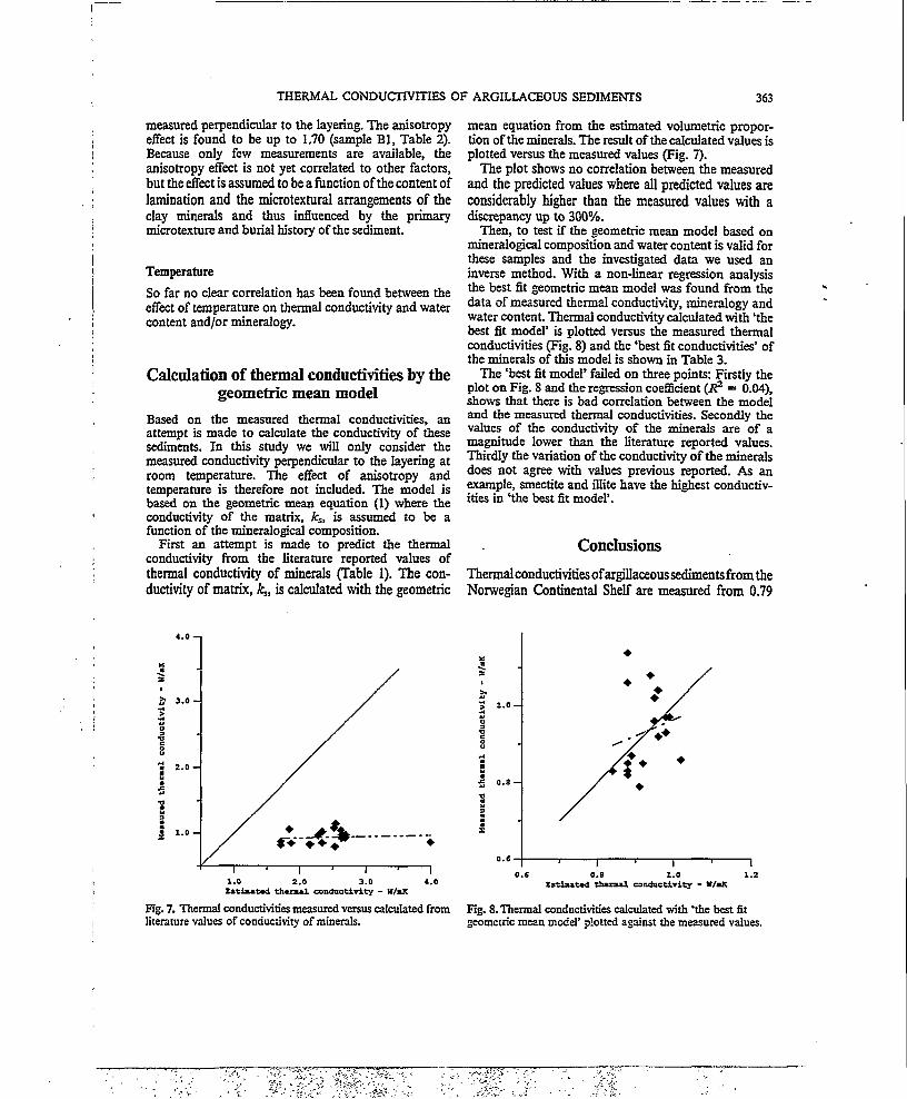
THERMAL CONDUCTIVITIES OF ARGILLACEOUS SEDIMENTS 363
measured perpendicular to the layering. The anisotropy effect is found to be up to 1.70 (sample Bl, Table 2). Because only few measurements are available, the anisotropy effect is not yet correlated to other factors, but the effect is assumed to be a function of the content of lamination and the microtextural arrangements of the clay minerals and thus influenced by the primary micro texture and burial history of the sediment.
TemperatureSo far no clear correlation has been found between the effect of temperature on thermal conductivity and water content and/or mineralogy.
Calculation of thermal conductivities by the geometric mean model
Based on the measured thermal conductivities, an attempt is made to calculate the conductivity of these sediments. In this study we will only consider the measured conductivity perpendicular to the layering at room temperature. The effect of anisotropy and temperature is therefore not included. The model is based on the geometric mean equation (1) where the conductivity of the matrix, ks, is assumed to be a function of the mineralogical composition.
First an attempt is made to predict the thermal conductivity from the literature reported values of thermal conductivity of minerals (Table 1). The conductivity of matrix, ks, is calculated with the geometric
4.0 -i
3.0 -
2.0 -
1.0 -
1.0 2.0 3.0Estimated thermal conductivity - H/nX
Fig. 7. Thermal conductivities measured versus calculated from literature values of conductivity of minerals.
mean equation from the estimated volumetric proportion of the minerals. The result of the calculated values is plotted versus the measured values (Fig. 7).
The plot shows no correlation between the measured and the predicted values where all predicted values are considerably higher than the measured values with a discrepancy up to 300%.
Then, to test if the geometric mean model based on mineralogical composition and water content is valid for these samples and the investigated data we used an inverse method. With a non-linear regression analysis the best fit geometric mean model was found from the data of measured thermal conductivity, mineralogy and water content. Thermal conductivity calculated with ‘the best fit model* is plotted versus the measured thermal conductivities (Fig. 8) and the ‘best fit conductivities' of the minerals of this model is shown in Table 3.
The ‘best fit model* failed on three points: Firstly the plot on Fig. 8 and the regression coefficient (It2, = 0.04), shows that there is bad correlation between the model and the measured thermal conductivities. Secondly the values of the conductivity of the minerals are of a magnitude lower than the literature reported values. Thirdly the variation of the conductivity of the minerals does not agree with values previous reported. As an example, smectite and illite have the highest conductivities in ‘the best fit model*.
Conclusions
Thermal conductivities of argillaceous sediments from the Norwegian Continental Shelf are measured from 0.79
1.0 -
Estimated thermal conductivity - W/aK
Fig. 8. Thermal conductivities calculated with ‘the best fit geometric mean model’ plotted against the measured values.

364 K. MIDTT0MME ET AL.
Table 3. The best fit values of thermalconductivity of the minerals
Minerals Thermalconductivity(W/mK)
Quartz 1.01Kaolinite 0.91ChloriteIllite 1.42SmectiteI/SPyrite 1.41Feldspar 1.02Carbonate
to 1.14W/mK. The thermal conductivity parallel to the layering is up to 1.70 higher than that perpendicular to the layering. The anisotropy effect may be of importance and taken into consideration when modelling in sedimentary basins with tilted strata.
The thermal conductivities presented in this work are lower than most data previously published. These earlier data have mainly been determined by needle probe techniques. The results are, however, comparable with thermal conductivities indirectly estimated from thermal studies of sedimentary basins (Blackwell & Steele 1989; Demon- godin et al. 1991; C. Hermanrud 1993 pens. comm.).
The water content is found to have some influence of thermal conductivities. The mineralogy seems to be less important for the conductivity. An attempt to calculate thermal conductivities with the geometric mean model, from the water content and the mineralogy was not successful. An explanation may be that the mineralogi- cal effect is lower for these fine grained sediments than for coarser samples.
Acknowledgements. The authors acknowledge the financial support provided by the Norwegian Research Council Grant D 440.91/026 and the CONOCO NORWAY Inc. project CNRD 25-6 on ‘Tertiary Claystones on the Norwegian Shelf.’ The study is also a contribution to the j oint University of Oslo/University of Trondheim R&D Programme on Clays Claystones and Shales in Petroleum Geology. The authors thank S. Lippard for correcting the English text and Joar Stettem, IKU Petroleum Research and an anonymous reviewer for very useful comments.
ReferencesAnand, J., Somerton, W.H. & Gomaa, E. 1973. Predicting
thermal conductivities of formations from other known properties. Society of Petroleum Engineers Journal, 267-273.
Balling, N., Kristiansen J. I., Breiner, N., Poulsen, K. D„ Rasmussen, R. & Saxov, S. 1981. Geothermal measurements and subsurface temperature modelling in Denmark. Geoskrifter, no. 16, Department of Geology, Aarhus University.
Blackwell, D. D. & Steele, J. L. 1989. Thermal conductivity of sedimentary rocks: Measurement and significance. In: Naeser, N.D&McCulloh, T. H. (eds) Thermal History of Sedimentary Basins: Methods and Case Histories. Springer, New York, 13-36.
Bloomer, J. R. 1981. Thermal conductivities of mudrocks in the United Kingdom. Quarterly Journal of Engineering Geology, 14, 357-362.
Brendeng, E. & Frivik, P. E. 1974. New development in design of equipment for measuring thermal conductivity and heat flow. Heat transmission measurements in thermal insulations, ASTM STP 544, American Society for Testing and Materials, 147-166.
Brigaud, F., Chapman, D. S. & LeDouaran, S. 1990. Estimating thermal conductivity in sedimentary basins using lithological data and geophysical well logs. AAPG Bulletin, 74, 1459-1477.
----- & Vasseur, G. 1989. Mineralogy, porosity and fluidcontrol on thermal conductivity of sedimentary rocks. Geophysical Journal, 98, 525-542.
Brindley, G. W & Brown, G. 1980 Crystal structures of clay minerals and their X-ray identification. Monograph no.5 Mineralogical Society, London.
Demongodin, L„ Pinoteau, B., Vasseur, G. & Gable, R. 1991. Thermal conductivity and well logs: A case study in the Paris Basin. Geophysical Journal International, 105, 675-691.
------ , Vasseur, G. & Brigaud, F. 1993. Anisotropy of thermalconductivity in clayey formations. In: Dore, A. G et al. (eds) Basin Modelling: Advances and Applications. Elsevier, Amsterdam, 209-217.
Farouki, O. T. 1981. Thermal Properties of Soils. CRREL Monograph 81-1.
Fjeldskaar, W., Mykkeltveit, J., Christie, O. H. J., Johansen, H., Langfeldt, J. M., Tyvand, P., Skurve, O. & Bjorkum, P. A. 1990. Interactive 2D Basin Modelling on Workstations. Proceedings SPE 20350 Petroleum Computer Conference, Denver Colorado, 181-196.
----- , Prestholm, E., Guargena, C. & Stephenson, M. 1993.Mineralogical and diagenetic control on the thermal conductivity of the sedimentary sequences in the Bjemaya Basin, Barents Sea. In: Dore, A. G et al. (eds) Basin Modelling: Advances and Applications. Elsevier, Amsterdam, 445-453.
Gilliam T. M. & Morgan, I. L. 1987. Shale: Measurement of Thermal Properties. Oak Ridge National Laboratory Report ORNL/TM-10499.
Horai, K. I. 1971. Thermal conductivity of rock-forming minerals. Journal of Geophysical Research, 76, 1278—1308.
Johansen, 0. 1975. Varmeledningsevne av Jordarter. Dr.ing. thesis, Department of Refrigeration Engineering, Norwegian Institute of Technology.
Moore, D. M. & Reynolds, R. C. 1989. X-ray Diffraction and the Identification and Analysis of Clay Minerals. Oxford University Press, New York.
Prestholm, E. & Fjeldskaar, W. 1993. Thermal conductivity in sedimentary rocks, and its bearing on basin temperature predictions, (abstr.) Supplement nr. 1, Terra Nova, 5, 655.
Roaldset, E. & Gjelsvik, N. 1993. Physical Properties of cap- rocks - Norwegian North Sea. Extended abstracts. European Association of Petroleum Geoscientists & Engineers 5th Conference and Technical Exhibition. Stavanger, Norway, 7-11 June 1993, F010.

THERMAL CONDUCTIVITIES OF ARGILLACEOUS SEDIMENTS 365
Rundberg, Y. 1991. Tertiary sedimentary history and basin evolution of the Norwegian North Sea between 60°— 6TN-an integrated approach. Bring thesis, Department of Geology and Mineral Resources Engineering, Norwegian Institute of Technology Rep. 25. Trondheim.
Somerton, W. H. 1992. Thermal properties and temperature related behavior of rock/fluid systems. Developments in Petroleum Sciences, 37, Elsevier, Amsterdam.
Tyridal, D. S. 1994. Litologisk og Mineralogisk Sammenset- ning av Slamslein i Relasjon til Loggrespons. Cand. sclent, thesis, Geology, University of Oslo, Oslo.
Woodside, W. & Messmer, J. H. 1961. Thermal conductivity of porous media. Journal of Applied Physics, 32,1688-1706.
ZHANG, J., Roaldset, E. & Lien, K. 1992. Cap rock properties for a North Sea reservoir, Proceedings 2nd. Lerkendal Petroleum Engineering Workshop, Trondheim, February 5-6,1992, 193-206.

Paper 3

Paper 3
Thermal conductivity of selected clay- and mudstones
from England*.
Kirsti Midttemme1, Elen Roaldsef and Per Aagaard2.
‘Department of Geology and Mineral Resources Engineering, Norwegian University of Science and Technology (NTNU), 7034 Trondheim, Norway.
“Department of Geology, University of Oslo, P.Box.1047, Blindem 0316 Oslo, Norway.
ABSTRACT
The clay- and mudstones investigated in this study are London Clay, Fullers Earth, Oxford Clay
and Kimmeridge Clay. Thermal conductivities of the samples were measured with a divided bar
apparatus. The values measured perpendicular to layering ranged from 0.68 to 0.97 W/m-K.
Comparative measurements of thermal conductivities were carried out by the needle probe method
and Middleton’s method. Deviation in the measured values up to 50% were obtained between the
needle probe and the divided bar method. The measurements were compared with values of thermal
conductivities estimated from the geometric mean model based on mineralogy and water content
These estimated values ranged from 0.87 to 2.01 W/m-K, which are considerably higher than the
measured values. A correlation is found between the grain size distributions of the samples and the
measured thermal conductivities. This textural effect on the thermal conductivity is assumed to be
the main reason for the low measured values and the lack of correlation between the measured and
the calculated values.
* In press. Clay Minerals, 33,131-145.
i
IF

2 Paper 3
INTRODUCTION.
Thermal conductivity is a physical property describing transfer of heat through the material. A
knowledge of thermal conductivity is important in understanding and modelling of the temperature in
sedimentary basins. Today there is still a lack of reliable information on sedimentary rocks, and
especially for clays, claystones and shales there are uncertainties related to the determination of
thermal conductivities (Blackwell & Steele, 1989; Brigaud & Vasseur, 1989; Demongodin et al., 1991;
Midttomme et al., 1997a). Different methods are used to measure thermal conductivity, where the two
main techniques are the stationary divided bar method and the transient needle probe method.
Comparative measurements between the two methods are previously reported and agreement was
obtained by Von Herzen & Maxwell (1959); Sass et al. (1971) and Brigaud & Vasseur (1989). Higher
values of thermal conductivity were measured with the needle probe by Slusarchuk & Foulger (1973),
Johansen (in Farouki, 1981), Somerton (1992) and Midttomme et al. (1997b.). The discrepancy in
these studies is in the range of 10 - 20 %.
Special problems related to the measuring of thermal conductivities of clays, claystones and shales
have resulted in less and probably poorer data available for these materials (Midttomme & Roaidset,
1997). The sampling and preparation of fine grained materials represents a major problem as the
material easily breaks up in the sampling process and even if successfully cored the samples might be
subjected to desiccation in laboratory conditions (Brigaud & Vasseur, 1989). The anisotropic structure,
which is generally observed for fine grained sediments, might be considered as a source of error in the
determination of thermal conductivity. The anisotropy of thermal conductivity is defined as the ratio
between thermal conductivity parallel to the layering, kn, and the one perpendicular, kj_. An anisotropy
of over 1.7 was measured for shales and clays (Fenner, 1963; Prestholm & Fjeldskaar, 1993;
Demongodin et al., 1993; Midttomme et al., 1997a). The measured anisotropy is probably affected by
the methods of measurement and sample preparation. In the divided bar method the heat is transferred
in a certain direction through the samples, while by the needle probe method the heat is more randomly
transferred. In other methods the samples are ground to a fine powder before the conductivity is
measured (Horai, 1971; Sass et al., 1971; Middleton, 1994). The effect of in-situ structure of the
samples is not taken into account by these methods.
Models are developed to estimate thermal conductivity from other material properties. Porosity is
considered to be of importance as pore fluids have lower thermal conductivity than the minerals (e.g.,
Gilliam & Morgan, 1987; Brigaud & Vasseur, 1989) (Table 1). A decrease in porosity will therefore
increase the thermal conductivity. In the lack of reliable and simple methods of measuring the porosity,
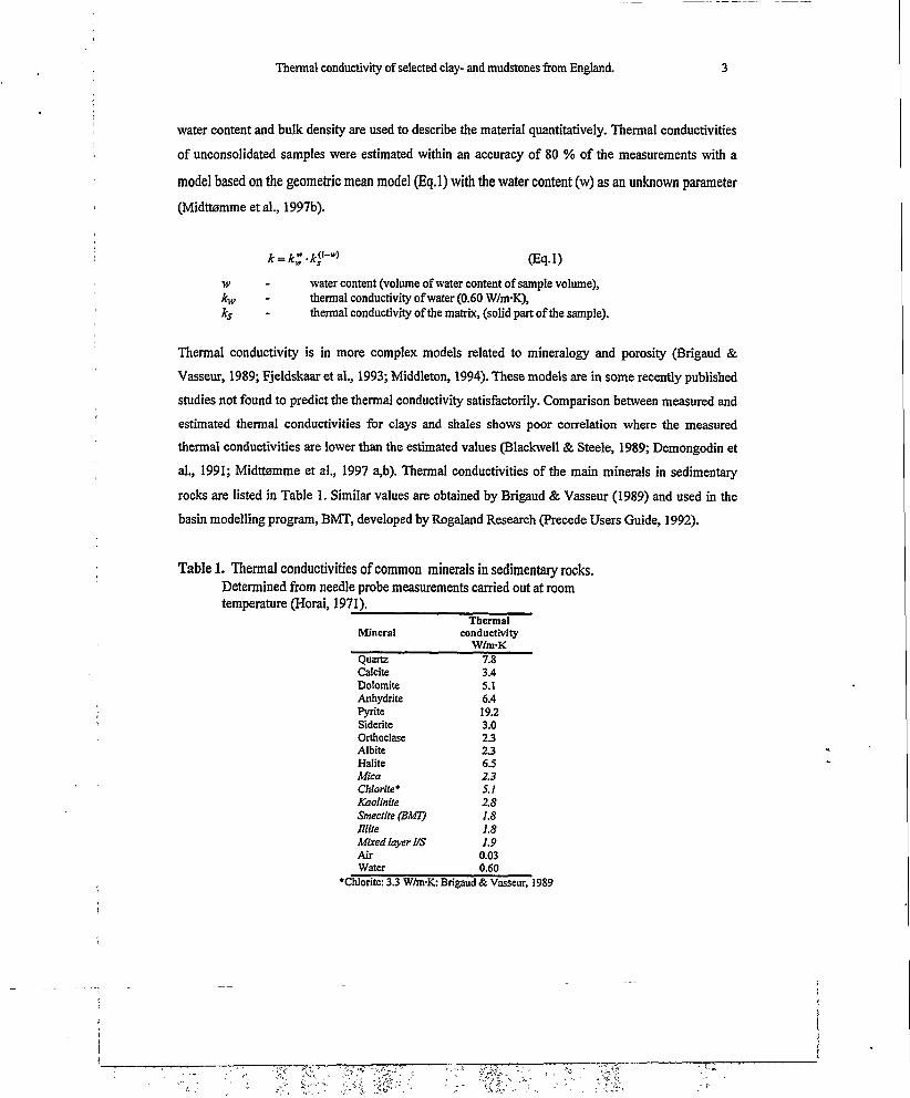
Thermal conductivity of selected clay- and mudstones from England. 3
water content and bulk density are used to describe the material quantitatively. Thermal conductivities
of unconsolidated samples were estimated within an accuracy of 80 % of the measurements with a
model based on the geometric mean model (Eq.l) with the water content (w) as an unknown parameter
(Midttemme et al., 1997b).
& = (Eq.l)
w - water content (volume of water content of sample volume),kw - thermal conductivity of water (0.60 W/m-K),ks - thermal conductivity of the matrix, (solid part of the sample).
Thermal conductivity is in more complex models related to mineralogy and porosity (Brigaud &
Vasseur, 1989; Fjeldskaar et al., 1993; Middleton, 1994). These models are in some recently published
studies not found to predict the thermal conductivity satisfactorily. Comparison between measured and
estimated thermal conductivities for clays and shales shows poor correlation where the measured
thermal conductivities are lower than the estimated values (Blackwell & Steele, 1989; Demongodin et
al., 1991; Midttemme et al., 1997 a,b). Thermal conductivities of the main minerals in sedimentary
rocks are listed in Table 1. Similar values are obtained by Brigaud & Vasseur (1989) and used in the
basin modelling program, BMT, developed by Rogaland Research (Precede Users Guide, 1992).
Table 1. Thermal conductivities of common minerals in sedimentary rocks. Determined from needle probe measurements carried out at room temperature (Horai, 1971). _______________________
MineralThermal
conductivityW/m-K
Quartz 7.8Calcite 3.4Dolomite 5.1Anhydrite 6.4Pyrite 19.2Siderite 3.0Orthoclase 2.3Albite 2.3Halite 6.5Mica 2.3Chlorite* 5.1Kaolinite 2.8Smectite (BMT) 1.8Illite 1.8Mixed layer VS 1.9Air 0.03Water 0.60
♦Chlorite: 3.3 W/m-K: Brigaud & Vasseur, 1989

4 Paper 3
The thermal conductivity is influenced by the texture of the material (e.g., Farouki, 1981; Brigaud &
Vasseur, 1989) and this might be a reason for this poor correlation between measured and estimated
thermal conductivities. The measured anisotropy of thermal conductivity is an example of this
influence, where a considerable variation in thermal conductivity is measured due to the direction of
heat flow through the material. Thermal conductivity is shown to depend on the grain size and grain
size distribution, where coarse grained materials have higher thermal conductivity than finer material
(Johansen, 1975; Beziat et al., 1992; Midttemme et al., 1997b.). From the conductivities presented in
Table 2 (Blackwell & Steele, 1989), it seems obvious that the grain size has great influence on thermal
conductivity.
Table 2. Thermal conductivities of sedimentary rocks at 20°C (Blackwell & Steele, 1989).
Lithology W/m-KClaystone and siltstone 0.80-1.25Shale 1.05-1.45Sand 1.70 - 2.50Sandstone 2.50-420
Beziat et al. (1992) found an increase in thermal conductivity with increasing content of sand in the
samples. They assumed this effect was due to the contact resistance between the grains. The resistance
decreases with increasing particle sizes as the number of contact points are reduced. In a study of
unconsolidated clays from the Voting Basin, offshore Norway, the effect of grain size fractions were
found to have greater influence on the measured thermal conductivities than the mineralogy
(Midttemme et al., 1997b).
Temperature and pressure are also found to influence thermal conductivity (e.g., Farouki, 1981;
Brigaud et al., 1990). The effect of these factors are negligible in the present study as all measurements
of thermal conductivities are carried out at nearly the same temperature and pressure.

Thermal conductivity of selected clay- and mudstones from England. 5
SCOTLAND
NORTH SEA
IRISH SEA
ENGLAND
WALES Lx
Figure 1. Map of the locations.
PRIABONIAN
BARTONIAN
LUTETIAN
YPRESIAN LONDON CLAY
SPARNACIAN
THANEHAN
DANIAN
MAASTRICHT! ANCAMPANIAN
SANTONIAN
CONIACIAN
TURONIAN
CENOMANIANLOWER
FULLERS EARTh]APTIAN
GREENSANDBARREMIAN
HAUTERIVIAN
VALANG1NIANRYAZANIAN
PORTLANDIANKIMMERIDGIAN KIMMERIDGE CLAYOXFORDIAN
CALLOVIAN I LOWER OXFORD CLAY
BATHONIAN
BAJOCIAN
AALENIAN
Figure 2. Stratigraphic position of the investigated clay- and mudstones.

6 Paper 3
GEOLOGICAL SETTINGS.
The claystones investigated in this study are London Clay, Fullers Earth, Oxford Clay and Kimmeridge
Clay (Figures 1,2). These onshore clay- and mudstones are well known and their material properties
have been extensively studied by Morris (1980), Huggett (1994), Kvilhaug (1995), Cartwright &
Lonergan (1996) and others. The clay- and mudstones were sampled in co-operation with Imperial
College, University of London in August 1992. The properties of these clay formations are of interest
in basin modelling because of their equivalence to offshore North Sea clay- and mudstones sequences.
The four clay- and mudstones are briefly described below and their macro and micro texture is shown
in Figure 3a-d. A more thorough description of the material is made in the report from the field work
and sampling (Kvilhaug et al., 1993; Kvilhaug, 1995). Particular characteristics of the clay- and
mudstones which might influence the thermal conductivity will be considered, in the following.
London Clay.
London Clay is a marine claystone of Eocene age which occurs as thick sequences in the Hampshire
and London Basins (Sellwood & Sladen, 1981) (Figure 3a). The clay was sampled at South Ockenden
pit, Essex, situated in the eastern part of the London Basin. The material can be characterized as a
laminated silty claystone, where thin silt laminae separate a relatively homogenous looking clay. The
distance between the silt laminas of this material is 5-20 cm. A detailed study of mineralogy and
diagenesis of the London Clay from South Ockenden is given by Huggett (1994). The formation has
been buried to a maximum of about 500 m, probably during the mid-Miocene tectonism which affected
southern England (Huggett, 1994). The clay is slightly overconsolidated due to Quaternary glacial load
(Kvilhaug et al., 1993).
Fullers Earth.
Fullers Earth is extreme in its composition by consisting mainly of Ca-smectite which is an alteration
product from volcanic ash (Figure 3b). The material was collected at Baulking Pit in Oxfordshire. This
clay is deposited as part of the Lower Greensand in Aptian-Albian time (Lower Cretaceous). The
claystone is stiff and overconsolidated with no visible structures. The maximum burial depth is
assumed to have been about 800 m (R. Marsden, pets, comm., 1992). Samples of Fullers Earth from
Reigate, Surrey, (in the Weald Basin) were also obtained. This claystone has a rusty weathering hue,
and seemed softer than the material from Baulking. However, other properties, such as texture, lack of
Thermal conductivity of selected clay- and mudstones from England. 7
structures and colour, seem almost identical for the two sites (Kvilhaug et al., 1993). The maximum
burial depth of this clay is estimated to 1000 m (R. Marsden, pers.comm. 1992).
Kimmeridge Clay.
Kimmeridge Clay is an organic rich, calcareous mudstone of Kimmeridgian age (Late Jurassic) that
crops out over large areas of southern and eastern England (Figure 3c). The Kimmeridge Clay, which
is equivalent to Draupne Formation, are known as the main hydrocarbon source rocks in the Central
and Northern North Sea (e.g., Grunau et al., 1986; Comford, 1990). The material of Kimmeridge Clay
was sampled at Westbury Quarry in Wiltshire. The material is a fissile mudstone with a well developed
lamination and visible strings of silt. The shale is rich in fossils, mostly shells. The samples were taken
from two different sites in the pit named A and B. The distance between the sites was about 100 m.
The samples from B were more consolidated. According to R. Marsden (pers. comm., 1992), the
material may have been buried to a depth of about 500 m.
Oxford Clay.
Lower Oxford Clay is an organic rich claystone of Callovian age (Middle Jurassic) that crops out over
large areas of southern and eastern England (Morris, 1980) (Figure 3d). It is of similar age as the North
Sea Heather Formation. It was sampled in Stewartby pit in Bedfordshire. The clay is rich in fossils,
mostly ammonites. The material is poorly laminated. Thickness of the eroded overburden of the
Oxford Clay is estimated to about 500 m (Jackson & Fookes, 1974).
Figure 3. Photographs and scanning electron microscopy micrographs of the clay-/ mudstones illustrating there macro- and micro texture. A) London Clay, B) Fullers Earth, (Note the
contact to the overlaying Lower Greensand). C) Kimmeridge Clay, D) Oxford Clay.
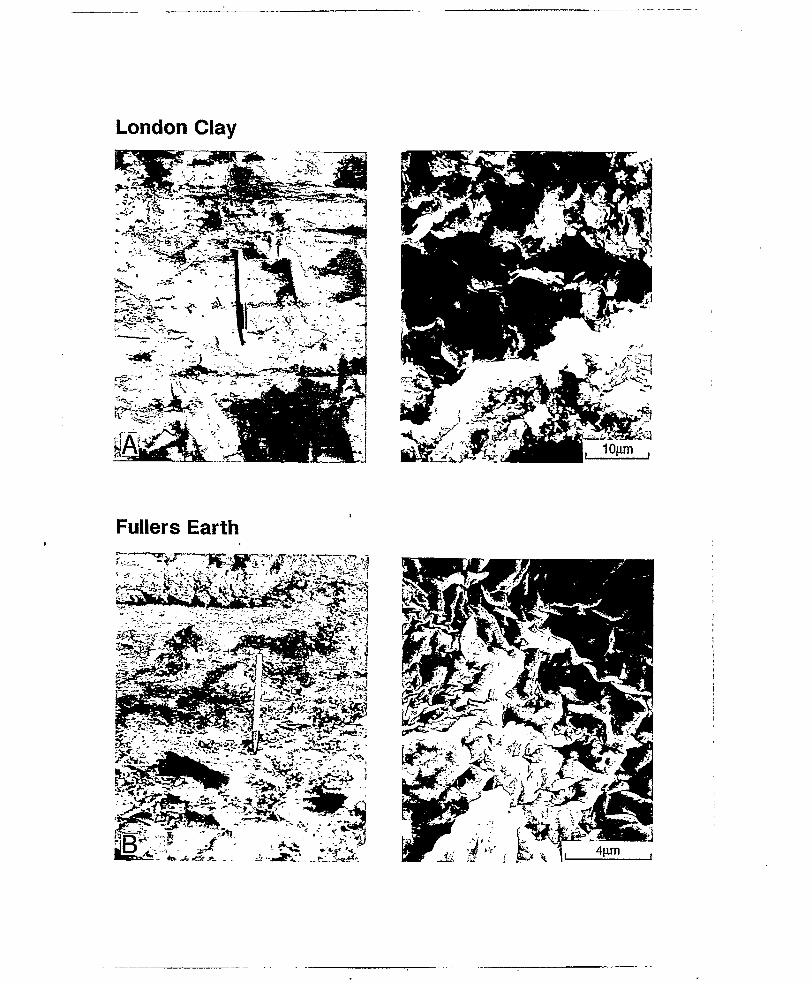
London Clay
Fullers Earth
j
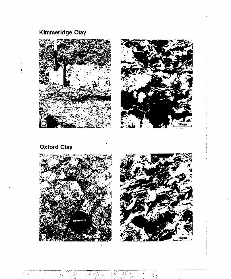
Kimmeridge Clay

10 Paper 3
PREVIOUS MEASUREMENTS OF THERMAL CONDUCTIVITIES.
Thermal conductivities of the four clay- and mudstones investigated in this study have been previously
reported by Bloomer (1981) (Table 3). This measurements were carried out with the needle probe
method and the divided bar apparatus on crushed samples by the method of Sass et al. (1971). Bloomer
(1981) investigated 12 mudstones from central southern England. The variation in thermal conductivity
was in the range 1.46 - 2.45 W/m-K, where the London Clay gave the highest values.
Table 3. Thermal conductivities measured by Bloomer (1981).
Sample Lithology Method No. of values
Thermalconductivity
W/m-KLondon Clay Sandy mudstone NPl 5 2.45 ±0.07Kimmeridge Clay Mudstone NP/PB2 58 1.51 ±0.09Oxford Clay Mudstone PB 11 1.57 ±0.03Fullers Earth Mudstone NP/PB 41 1.95 ±0.05
'Needle Probe measurement - The values of thermal conductivity are assumed to be the value parallel to the bedding (Bloomer, 1981).
2Phil box measurement (Sass method ) (Sass et al., 1971) Divided bar measurements on crushed sample. The values obtained are assumed to be a mean value of perpendicular and parallel thermal conductivities.
METHODS.
Measurement of thermal conductivities.
Thermal conductivity was measured with a divided bar apparatus. This is a steady state method, where
thermal conductivity is determined when the temperature gradient of the sample is constant and
controlled. The apparatus used is developed at Department of Refrigeration Engineering, Norwegian
University of Science and Technology, and is described in detail by Brendeng & Frivik (1974). Our
measurements were carried out on water saturated cubes with sides of 3.0 cm. Tests show that because
of the small size of the samples the measured values are up to 3.5 % lower than for bigger samples.
Thermal conductivity was measured both perpendicular (kjJ and parallel (kn) to the layering.
The needle probe measurements were carried out at University of Aarhus, Denmark. This transient
method was developed by Von Herzen & Maxwell (1959) and is today the most common laboratory
method for measurement of thermal conductivity (Jessop, 1990). A probe, which contains a heating
wire and a thermistor, is inserted into the material. When the system has attained temperature
equilibrium, the temperature is recorded as a function of time. From this temperature-time curve the

Thermal conductivity of selected clay- and mudstones from England. 11
thermal conductivity of the material can be determined (Jessop, 1990). Thermal conductivity parallel
to the layering was measured by inserting the probe perpendicular to the layering. Thermal
conductivity perpendicular to layering was calculated from the "results of inserting the probe parallel
and perpendicular to the layering (conf. Penner, 1963).
The third method, which is also a transient method has been developed by Middleton (1993) at
Chalmers University, Sweden. The apparatus is similar to the divided bar apparatus where a constant
heat flow is induced from the top of the sample, a block of size 4.0 • 4.0 cm2 and height 1.0 cm. The
sample is insulated on all other surfaces. The temperature is measured at the base of the sample for
about 60 seconds after introduction of the heat source (Middleton, 1993). Thermal conductivity can be
estimated from the temperature-time plot from the similar equations as for the needle probe method.
Other laboratory investigations.
The mineralogical composition of the samples was determined by X-ray diffraction analysis (Brindley
& Brown, 1980; Moore & Reynolds, 1989). The mineralogy was quantified by calculating the areas of
the characteristic peaks and applying weighting factors developed for the XRD equipment at
Department of Geology and Mineral Resources Engineering, Norwegian University of Science and
Technology by H.G. Rueslatten. The quantification is considered to be semi-quantitative with average
error in the order of 5-10 % (Rundberg, 1991).
The problem of porosity determinations in shales and claystones has among others been discussed by
Truman et al. (1989). With reference to some of the discussion by him and others, porosity was
determined by weighing water saturated samples of known volume before and after drying at 40 °C for
two weeks and then recalculate the water loss to water volume (i.e. porosity)- By this method the “free
water” which also may be considered as a measure for the “effective porosity” is determined. This
method is not any standard method, but from laboratory investigations of smectitic samples carried out
at this Department the transformation to illite has for some samples started at temperatures above 40
°C. Bound water is, by the definition of porosity (North, 1985) not included either in the effective or
the total porosities. Total water content was calculated from weight reduction after drying for 3 days at
105 °C.
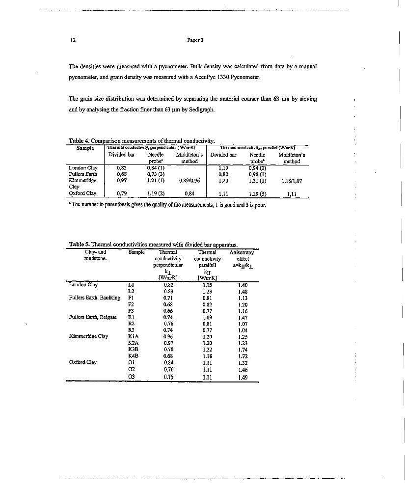
12 Paper 3
The densities were measured with a pycnometer. Bulk density was calculated from data by a manual
pycnometer, and grain density was measured with a AccuPyc 1330 Pycnometer.
The grain size distribution was determined by separating the material coarser than 63 pm by sieving
and by analysing the fraction finer than 63 pm by Sedigraph.
Table 4. Comparison measurements of thermal conductivity.Sample Thermal conductivity, perpendicular (W/m-K)
Divided bar Needle Middleton’sprobe* method
Thermal conductivity, parallel (W/m-K)
Divided bar Needle Middleton’sprobe* method
London Clay 0,83 0,84(1) 1,19 0,94(3)Fullers Earth 0,68 0,73 (3) 0,80 0,98 (1)Kimmeridge 0,97 1,21 (1) 0,89/0,96 1,20 1,21 (1) 1,18/1,07ClayOxford Clay 0,79 1,19(2) 0,84 1,11 1.29(3) 1,11
* The number in parenthesis gives the quality of the measurements, 1 is good and 3 is poor.
Table 5. Thermal conductivities measured with divided bar apparatus.Clay- andmudstone.
Sample Thermalconductivity
perpendiculark±
[W/m-K]
Thermalconductivity
parallel!kII
[W/m-K]
Anisotropyeffect
a=kjj/kj_
London Clay LI 0.82 1.15 1.40L2 0.83 1.23 1.48
Fullers Earth, Baulking FI 0.71 0.81 1.13F2 0.68 0.82 1.20F3 0.66 0.77 1.16
Fullers Earth, Reigate R1 0.74 1.09 1.47R2 0.76 0.81 1.07R3 0.74 0.77 1.04
Kimmeridge Clay K1A 0.96 1.20 1.25K2A 0.97 1.20 1.23K3B 0.70 1.22 1.74K4B 0.68 1.18 1.72
Oxford Clay 01 0.84 1.11 1.3202 0.76 1.11 1.4603 0.75 1.11 1.49

Thermal conductivity of selected clay- and mudstones from England. 13
COMPARISONS OF THERMAL CONDUCTIVITY MEASUREMENTS.
All measurements of thermal conductivities presented in this study (Tables 4, 5) are lower than the
measurements carried out by Bloomer (Table 3). Bloomer’s measurements for London Clay and
Fullers Earth appear to be more than twice as high as the measurements carried out in this study. The
discrepancy in the measurements for Fullers Earth is most disquieting since this clay appears to be
nearly homogenous and isotropic. The discrepancy can therefore hardly be due to mineralogical nor
textural variations of the measured samples. London Clay was by Bloomer classified as sandy
mudstone. Our measurements were carried out on a claystone with a content of silt and sand of 30%
and 10% respectively. Lithological differences between the samples analysed might thus be a reason
for this discrepancy. Regarding this comparison, it is noteworthy that the measurements by Bloomer
(1981) and the University of Aarhus were both carried out by the needle probe method (see Tables 3,
4). The discrepancy between these results shows that there might be considerable disagreement in
measurements carried out by the same method.
For the samples investigated in the present study there are also some disagreements in the comparative
measurements of the three methods (Table 4). The measurements with the method developed by
Middleton (1993) and the divided bar apparatus are in good agreement, while in general the needle
probe method gives higher values. Of the eight measurements, the needle probe gives higher thermal
conductivity for five of the samples (+7 % - +51 %) and lower for the parallel measurements of
London Clay (-21%). Two of the measurements are in agreement (+1 %). It is difficult from these
comparative measurements, because of the variation and also the limitation of measurements, to
confirm if there is methodical discrepancy between the two methods as previously suggested by
Slusarchuk & Foulger (1973); Farouki (1981) and Midttemme et al. (1997b). The measurements
perpendicular to the layering for the organic rich Kimmeridge Clay and Oxford Clay show the highest
deviation between the needle probe and the two other methods (Table 4). Thermal conductivity
measured parallel to the layering for these two clays, and particular for the Kimmeridge Clay, are in
good agreement. The results of the measurements on the organic rich clays give a low or no anisotropy
of the thermal conductivity by the needle probe methods, while a considerable anisotropy is measured
by the two other methods. A high content of fossil and shell debris with a clear orientation parallel to
the layering were easily seen in these two mudstones. The needle probe method differs from the other
methods in the way the heat is transferred through the sample. By this method the heat is transferred
radially from a probe inserted into the sample. For the apparatus developed by Middleton, and the
divided bar apparatus, the heat is transferred from a slab through the sample (Figure 4). In the divided

14 Paper 3
bar method great emphasis is made to obtain controlled and stationary conditions of the heat flow
through the samples. The shell and fossil debris, with preferred orientation in the two organic rich
clays might be an explanation of the deviation in the perpendicular measurements with the needle
probe method. Because the heat flow is radiated from a line source, the fossil and shell debris might
also strongly influence the thermal conductivity measured perpendicular to the layering. This influence
might also explain the lack of anisotropy of the measured conductivities for the organic rich clays
carried out with this method.
Divided bar method
Needle probe method
Figure 4. Heat flow through the samples during the thermal conductivity measurements.Tj and T% designate the high and low temperature, while q represents the heat flow indicated by the arrows.

Thermal conductivity of selected clay- and mudstones from England. 15
THE EFFECT OF MATERIAL PARAMETERS ON THE THERMAL CONDUCTIVITY.
Two or three samples of each of the clays- and mudstones were prepared and measured with the
divided bar apparatus. The thermal conductivity was measured on water saturated samples both
perpendicular and parallel to the layering, as shown in Table 5. The mineralogical composition and the
physical properties of the material are shown in Tables 6 and 7. In sedimentary basins the dominating
heat mechanism is the conductive heat transferred from the Earth’s interior through the crust. For this
reason the perpendicular values of the thermal conductivities measured and are used in the following.
This measured thermal conductivities varies in the range of 0.66 W/m-K to 0.97 W/m-K for the
samples of the four clay- and mudstones. These values of thermal conductivities will be correlated with
the mineralogical, physical and textural properties of the samples, and the influence of these properties
on the thermal conductivity will be discussed.
Table 6. Mineralogy of the samples.Sample Quartz Pyrite Feldspar Calcite Dolom Siderite Gypsum Aragon Kaolin. Elite Smect us
London Clay 37 2 18 2 13 16 5 7Fullers Earth, Baulking 2 3 95Fullers Earth, Reigate 2 3 95Kimmeridge Clay, A 18 2 3 62 2 4 4 6Kimmeridge Clay, B 42 11 7 5 2 8 13 14Oxford Clay 34 9 6 16 13 22
Table 7. Densities, porosity, water content and grain size fractions of the samples.Sample Grain density
g/cm3Bulk density
g/cm3Porosity
%ofvolume
Watercontent
%ofvolume
Clayfraction
%ofweight
Siltfraction
%ofweight
Sandfraction
%ofweight
London Clay 2.64 1.95 37 48 58 33 9Fullers Earth, Baulking 2.42 1.69 65 85 15Fullers Earth, Reigate 2.41 50 85 15 -
Kimmeridge Clay, A 2.57 2.27 34 35 44 40 16Kimmeridge Clay, B 2.60 1.94 37 45 65 34 1Oxford Clay 2.54 1.94 42 40 44 46 10
Figure 5. Thermal conductivity plotted versus: a) porosity, b) water content, c) bulk and d) grain densities.The linear regression lines are shown.
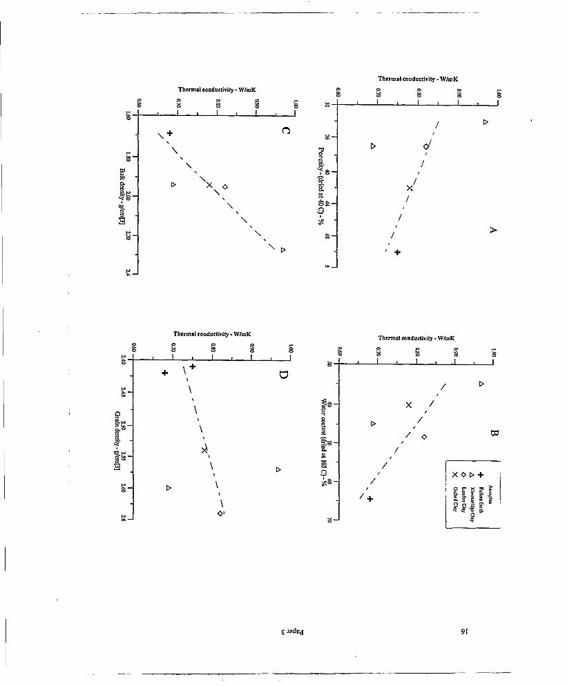
Thermal conductivity - W/mK
Thermal conductivity - W/mK
S § 1 I §
Thermal conductivity - W/mK
1 I I I IThermal conductivity - W/mK
1 § I 1 i
x o > +
S-raded 91
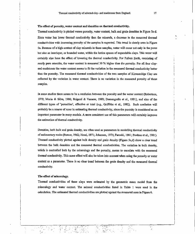
Thermal conductivity of selected clay- and mudstones from England. 17
The effect of porosity, water content and densities on thermal conductivity.
Thermal conductivity is plotted versus porosity, water content, bulk and grain densities in Figure 5a-d.
Since water has lower thermal conductivity than the minerals, a decrease in the measured thermal
conductivities with increasing porosity of the samples is expected. This trend is clearly seen in Figure
5a. Because of a high content of clay minerals in these samples, water will occur not only in the pores
but also as interlayer, or bounded water, within the lattice spaces of expandable clays. This water will
certainly also have the effect of lowering the thermal conductivity. For Fullers Earth, consisting of
nearly pure smectite, the water content is measured 30 % higher than the porosity. For all four clay-
and mudstones the water content seems to fit the variation in the measured thermal conductivity better
than the porosity. The measured thermal conductivities of the two samples of Kimmeridge Clay are
reflected by the variation in water content. There is no variation in the measured porosity of these
samples.
In some studies there seems to be a confusion between the porosity and the water content (Robertson,
1979; Morin & Silva, 1986; Brigaud & Vasseur, 1989; Demongodin et al., 1991), and also of the
different types of ‘porosities’, effective or total (e.g., Griffiths et al., 1992). Such confusion will
probably be a source of error in estimating thermal conductivity, since the porosity is considered as an
important parameter in many models. A more consistent use of this parameters will certainly improve
the estimation of thermal conductivity.
Densities, both bulk and grain density, are often used as parameters in modelling thermal conductivity
of sedimentary rocks (Fenner, 1962; Horai, 1971; Johansen, 1975; Farouki, 1981; Poulsen et al., 1981).
Thermal conductivity plotted against bulk density and grain density (Figure 5c,d) show a clear trend
between the bulk densities and the measured thermal conductivities. The variation in bulk density,
which is controlled both by the mineralogy and the porosity, seems to correlate with the measured
thermal conductivity. This same effect will also be taken into account when using the porosity or water
content as a parameter. There is no clear trend between the grain density and the measured thermal
conductivity.
The effect of mineralogy.
Thermal conductivities of these clays were estimated by the geometric mean model from the
mineralogy and water content. The mineral conductivities listed in Table 1 were used in the
calculation. The estimated thermal conductivities are plotted against the measured ones in Figure 6.

18 Paper 3
2.00-
I
> 1.60-
3■as
120 —
0.80 —
Samples
o London Clay
+ Fullers Earth
A Kimmeridge Clay
X Oxford Clay
&
_-X--
0.80 120 1.60 200 Estimated thermal conductivity - W/mK
Figure 6. Calculated thermal conductivity versus measured thermal conductivity. The solid line is the unity line (1:1). The dotted line is the regression line.
If the measurements of thermal conductivities are correct, this mineralogical model fails to estimate
the thermal conductivity of these samples. As seen in Figure 6, the estimated thermal conductivities for
all of the samples are considerably higher than the measured values. The value of the thermal
conductivity of the Kimmeridge Clay is an example of the lack of correlation with the mineralogy. Of
the minerals present, pyrite and quartz have high thermal conductivity (Table 1). Samples with a high
content of these minerals are expected to have higher thermal conductivity. The sample from site A has
a content of quartz and pyrite of 18 and 2 % respectively, while the sample from site B has a quartz
content of 44 % and a pyrite content of 11 %. From the mineralogy the thermal conductivity of sample
B is predicted to be higher than that of sample A. The measurements however show the opposite, as the
thermal conductivity of sample A is 40 % higher than of the sample B, 0.97 W/m-K and 0.69 W/m K
respectively.

Thermal conductivity of selected clay- and mudstones from England. 19
A thermal conductivity of 0.68 W/m-K is measured for Fullers Earth. This value is only 13 % higher
than for pure water. Because of the homogeneity of this clay there is low uncertainty related to the
determination of the mineralogy. The mineral conductivity of smectite is 1.8 W/m-K (Table 1). To
calculate a bulk thermal conductivity of 0.68 W/m-K with the geometric mean model (Eq.l), the matrix
conductivity of Fullers Earth is estimated to 0.77 W/m-K or 0.86 W/m-K if the bounded water is
excluded. A possible explanation for the lack of correlation between the measured thermal
conductivities and the mineralogy for Fullers Earth is that the mineral conductivity of this authigenic
formed Ca- smectite is much lower than the values previously reported for smectite.
Another explanation for these low values measured on Fullers Earth, and also for the three other clays,
is that there are other material parameters in addition to mineralogy which have strong influence on the
thermal conductivities of these samples.
Samples
+ Fullers Earth
A KimmeridgeCIay
O London Clay
X Oxford Clay
v )
Clay fraction (0.002mm) %
Figure 7. The clay traction (< 2pm) of the samples plotted versus the sand fraction (> 63pm). The measured thermal conductivity is shown.
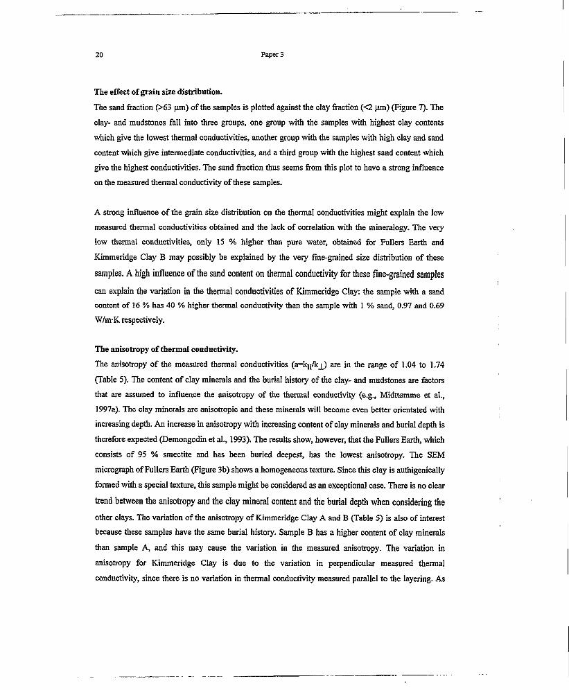
20 Paper 3
The effect of grain size distribution.
The sand fraction (>63 pm) of the samples is plotted against the clay fraction (<2 pm) (Figure 7). The
clay- and mudstones fall into three groups, one group with the samples with highest clay contents
which give the lowest thermal conductivities, another group with the samples with high clay and sand
content which give intermediate conductivities, and a third group with the highest sand content which
give the highest conductivities. The sand fraction thus seems from this plot to have a strong influence
on the measured thermal conductivity of these samples.
A strong influence of the grain size distribution on the thermal conductivities might explain the low
measured thermal conductivities obtained and the lack of correlation with the mineralogy. The very
low thermal conductivities, only 15 % higher than pure water, obtained for Fullers Earth and
Kimmeridge Clay B may possibly be explained by the very fine-grained size distribution of these
samples. A high influence of the sand content on thermal conductivity for these fine-grained samples
can explain the variation in the thermal conductivities of Kimmeridge Clay: the sample with a sand
content of 16 % has 40 % higher thermal conductivity than the sample with 1 % sand, 0.97 and 0.69
W/m-K respectively.
The anisotropy of thermal conductivity.
The anisotropy of the measured thermal conductivities (a=kn/kj_) are in the range of 1.04 to 1.74
(Table 5). The content of clay minerals and the burial history of the clay- and mudstones are factors
that are assumed to influence the anisotropy of the thermal conductivity (e.g., Midttemme et al.,
1997a). The clay minerals are anisotropic and these minerals will become even better orientated with
increasing depth. An increase in anisotropy with increasing content of clay minerals and burial depth is
therefore expected (Demongodin et al., 1993). The results show, however, that the Fullers Earth, which
consists of 95 % smectite and has been buried deepest, has the lowest anisotropy. The SEM
micrograph of Fullers Earth (Figure 3b) shows a homogeneous texture. Since this clay is authigenically
formed with a special texture, this sample might be considered as an exceptional case. There is no clear
trend between the anisotropy and the clay mineral content and the burial depth when considering the
other clays. The variation of the anisotropy of Kimmeridge Clay A and B (Table 5) is also of interest
because these samples have the same burial history. Sample B has a higher content of clay minerals
than sample A, and this may cause the variation in the measured anisotropy. The variation in
anisotropy for Kimmeridge Clay is due to the variation in perpendicular measured thermal
conductivity, since there is no variation in thermal conductivity measured parallel to the layering. As

Thermal conductivity of selected clay- and mudstones from England. 21
previously suggested the very low perpendicular thermal conductivity measured for Kimmeridge Clay
B might be due to the very fine grain size distribution of this sample. The fact that there is low
variation in the parallel measurements for both the organic-rich clays, Kimmeridge Clay and Oxford
Clay, suggests that the organic material has a strong effect on the thermal conductivity. The strong
anisotropic effect measured on the samples from site B of Kimmeridge Clay is therefore assumed to be
due to textural effects, in this case due to a very fine grain size distribution and a high content of
organic material parallel to the bedding.
CONCLUSIONS.
Thermal conductivities measured on four selected clay- and mudstones with the divided bar apparatus
are in the range of 0.66 W/m-K to 0.97 W/m-K. These results are lower than previous measurements on
these clays by Bloomer (1981). The grain size distribution of the samples shows a good correlation
with the measured thermal conductivities as the sample with the highest sand content has the highest
thermal conductivity, and samples with highest clay contents have lowest thermal conductivities.
Correlation is also observed between the thermal conductivities and porosity, water content, and bulk
density. The water content seems to reflect the variations in the measured conductivities better than the
porosity. No clear trend could be observed between the grain density and thermal conductivity.
Comparative measurements carried out with the needle probe method and the method developed by
Middleton, demonstrated some disagreements between the needle probe method and the two other
methods. For the organic rich mudstones this discrepancy in the measurements is suggested to reflect
methodical variation in the direction of heat flow through the sample during measurement.
Thermal conductivities of the clay- and mudstones, estimated by the geometric mean model from
water content and mineralogy, were considerably higher than the measured values. The very fine
grained nature of these clay- and mudstones are assumed to be the reason for the extremely low
measured thermal conductivities, and the lack of correlation with the mineralogically based model.
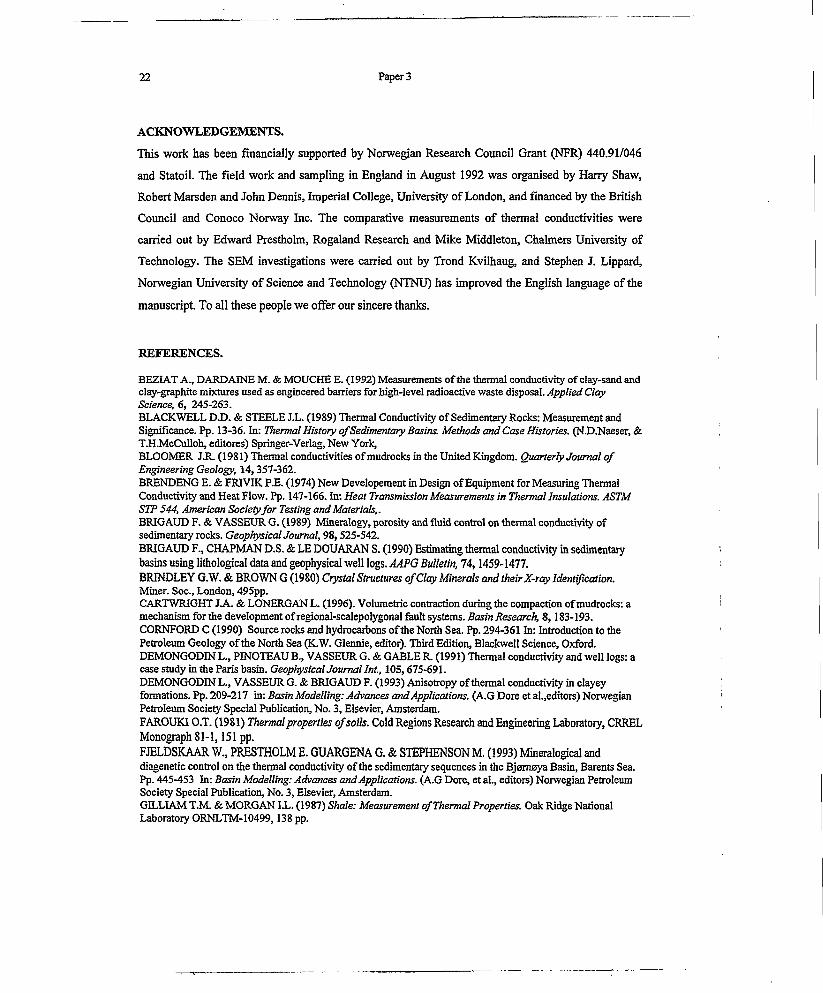
22 Paper 3
ACKNOWLEDGEMENTS.
This work has been financially supported by Norwegian Research Council Grant (NFR) 440.91/046
and Statoil. The field work and sampling in England in August 1992 was organised by Harry Shaw,
Robert Marsden and John Dennis, Imperial College, University of London, and financed by the British
Council and Conoco Norway Inc. The comparative measurements of thermal conductivities were
carried out by Edward Prestholm, Rogaland Research and Mike Middleton, Chalmers University of
Technology. The SEM investigations were carried out by Trond Kvilhaug, and Stephen J. Lippard,
Norwegian University of Science and Technology (NTNU) has improved the English language of the
manuscript. To all these people we offer our sincere thanks.
REFERENCES.
BEZIAT A., DARDAINE M. & MOUCHE E. (1992) Measurements of the thermal conductivity of clay-sand and clay-graphite mixtures used as engineered barriers for high-level radioactive waste disposal. Applied Clay Science, 6, 245-263.BLACKWELL D.D. & STEELE J.L. (1989) Thermal Conductivity of Sedimentary Rocks: Measurement and Significance. Pp. 13-36. In: Thermal History of Sedimentary Basins. Methods and Case Histories. (N.D.Naeser, & T.H.McCulloh, editores) Springer-Verlag, New York,BLOOMER J.R. (1981) Thermal conductivities of mudrocks in the United Kingdom. Quarterly Journal of Engineering Geology, 14,357-362.BRENDENG E. & FRIVIK P.E. (1974) New Developement in Design of Equipment for Measuring Thermal Conductivity and Heat Flow. Pp. 147-166. In: Heat Transmission Measurements in Thermal Insulations. ASTM STP 544, American Societyfor Testing and Materials,.BRIGAUD F. & VASSEUR G. (1989) Mineralogy, porosity and fluid control on thermal conductivity of sedimentary rocks. Geophysical Journal, 98,525-542.BRIGAUD F., CHAPMAN D.S. & LE DOUARAN S. (1990) Estimating thermal conductivity in sedimentary basins using lithological data and geophysical well logs. AAPG Bulletin, 74,1459-1477.BRINDLEY G.W. & BROWN G (1980) Crystal Structures of Clay Minerals and their X-ray Identification. Miner. Soc., London, 495pp.CARTWRIGHT JA. & LONERGAN L. (1996). Volumetric contraction during the compaction of mudrocks: a mechanism for the development of regional-scalepolygonal fault systems. Basin Research, 8, 183-193. CORNFORD C (1990) Source rocks and hydrocarbons of the North Sea. Pp. 294-361 In: Introduction to the Petroleum Geology of the North Sea (K.W. Glennie, editor). Third Edition, Blackwell Science, Oxford. DEMONGODIN L., PINOTEAU B., VASSEUR G. & GABLE R. (1991) Thermal conductivity and well logs: a case study in the Paris basin. Geophysical Journal Int., 105,675-691.DEMONGODIN L., VASSEUR G. & BRIGAUD F. (1993) Anisotropy of thermal conductivity in clayey formations. Pp. 209-217 in: Basin Modelling: Advances and Applications. (A.G Dore et al.,editors) Norwegian Petroleum Society Special Publication, No. 3, Elsevier, Amsterdam.FAROUKI O.T. (1981) Thermal properties of soils. Cold Regions Research and Engineering Laboratory, CRREL Monograph 81-1,151 pp.FJELDSKAAR W., PRESTHOLM E. GUARGENA G. & STEPHENSON M. (1993) Mineralogical and diagenetic control on the thermal conductivity of the sedimentary sequences in the Bjomaya Basin, Barents Sea. Pp. 445-453 In: Basin Modelling: Advances and Applications. (A.G Dore, et al., editors) Norwegian Petroleum Society Special Publication, No. 3, Elsevier, Amsterdam.GILLIAM T.M. & MORGAN I.L. (1987) Shale: Measurement of Thermal Properties. Oak Ridge National Laboratory ORNLTM-10499,138 pp.

Thermal conductivity of selected clay- and mudstones from England. 23
GRIFFITHS C.M., BRERETON N.R., BEAUSILLON R. & CASTILLO D. (1992) Thermal conductivity prediction from petrophysical data: a case study. In: Geological Applications of Wireline Logs II (A. Hurst, C.M. Griffiths, P.F. Worthington, editors), Geological Society Special Publication, No. 65, 299-315.GRUNAU H.R., BLASER R., MOSER H.J. & ZIEGLER U. (1986) Overview of cap rocks for hydrocarbon accumulations. Vol. 1-6, Petroconsultants s.a., Geneva.HORAIK. (1971) Thermal conductivity of rock-forming minerals. Journal of Geophysical Research, 76, 1278- 1308.HUGGETT J.M. (1994) Diagenesis of Mudrocks and Concretions from the London Clay Formation in the London Basin Clay Minerals, 29,693-707.JACKSON J.O. & FOOKES P.G. (1974) The relationship of the estimated former burial depth of the lower Oxford Clay to some soil properties. The Quarterly Journal of Engineering Geology, 7,137-181.JESSOP A.M. (1990) Thermal Geophysics. Developements in Sollid Earth Geophysics 17, Elsevier, 306 pp. JOHANSEN 0. (1975) Varmeledningsevne av jordarter. Dr. ing thesis, Department of Refrigeration Engineering, Norwegian Institute of Technology, Trondheim, 231 pp. (Thermal conductivity of soils,Cold Region Research and Engineering Laboratory, CRREL Draft Translation 637,1977 ADA 044002). KVILHAUG T. (1995) Rock mechanical properties ofmudstone in relation to petrology. Dr.ing. thesis, 1995:90, Nowegian University of Science and Technology, Trondheim.KVILHAUG T., MIDTT0MME K. & ROALDSET E. (1993) Petrology and physical properties ofclays and mudrocks. Field work and sampling in Great Britain - August 1992. Research programme on clays, claystones and shales in petroleum geology. Report No.36. Norwegian Institute of Technology, Trondheim, 41 pp. MIDDLETON M. (1993) A transient method of measuring the thermal properties of rocks. Geophysics, 58, 357-365.MIDDLETON M (1994) Determination of matrix thermal conductivity from dry drill cuttings. AAPG Bulletin,78,1790-1799.MIDTT0MME K., ROALDSET E. & AAGAARD P. (1997a) Thermal conductivities of argillaceous sediments. Pp. 131-140 In: Modern Geophysics in Engineering Geology. ( D.M McCann, et al., editors). Geological Society Engineering Geology Special Publication, 12,357-365.MIDTT0MME K., SjETTEM J. & ROALDSET E. (1997b) Thermal conductivity of unconsolidated sediments from the Voting Basin, Norwegian Sea. (M.Middleton, editor) Nordic Petroleum Technology Series, 2, Nordisk energiforskningssamarbejde.MIDTT0MME K. & ROALDSET E. (1997) The influence of clay minerals on thermal conductivity of sedimentary rocks.Nordiskforeningfor lerforskning, Meddelandenr. 11.MORIN R. & SILVA A.J. (1984) The effects of high pressure and high temperature on some physical properties of ocean sediments. Journal of Geophysical Research, 89,511-526.MOORE D.M. & REYNOLDS R.C. (1989) X-ray Diffraction and the Identification and Analysis of Clay Minerals. Oxford Univ. Press, New York, 332 pp.MORRIS K.A. (1980) Comparison of major sequences of organic-rich mud deposition in the British Jurassic. Journal of Geological Society, London, 137,157-170.NORTH F.K. (1985) Petroleum Geology. Unwin Hyman Inc. Second Impression, 630 pp.PENNER E. (1962) Thermal conductivity of saturated Leda clay. Geotechnique, 12,168-175.PENNER E. (1963) Anisotropic thermal conduction in clay sediments. Proceedings, International Clay Conference, Stockholm, vol.l, 365-376, Pergamon Press, Elmsford.POULSEN K.D., SAXOV S., BALLING N. & KRISTIANSEN J.I. (1981) Thermal conductivity measurements on Silurian limestones from tire Island of Gotland, Sweden. Geologiske Forening i Stockholm Forhandlingar, 103,349-356.PRECEDE USERS GUIDE (1992) Thermal conductivity prediction tool, Version 1.1.Precede™, ProCom a.s, Stavanger Norway, 14 pp.PRESTHOLM E. & FJELDSKAAR W. (1993) Thermal conductivity anisotropy in sedimentary rocks, and it’s bearing on basin temperature predictions. European Union of GeologyVII Strasbourg, France 1993 Abstract Supplement, No.l to Terra Nova, 5, 655.ROBERTSON E.C. (1979) Thermal conductivity of rocks. Open File Report 79-356. United States Department of the Interior, U.S Geological Survey, 30 pp.RUNDBERG Y. (1991) Tertiary sedimentary history and basin evolution of the Norwegian North Sea between

24 Paper 3
60 °- 62°N-an integrated approach. Dr. ing. thesis, Department of Geology and Mineral Resources Engineering, Norwegian Institute of Technology, Rep. 25. Trondheim, 291 pp.SASS J.H., LACHENBRUCH A.H. & MUNROE R. J. (1971) Thermal conductivity of rocks from measurements of fragments and its application to heat-flow determinations. Journal of Geophysical Research, 76,3391-3401. SELLWOOD B.W. & SLADEN C.P. (1981) Mesozoic and Tertiary argillaceous units: distribution and composition. Quarterly Journal of Engineering Geology, 14, 263-275.SLUSARCHUK W.A. & FOULGER P.H. (1973) Develoment and calibration ofa thermal conductivity probe apparatus for use in the field and laboratory. National Research Council of Canada, Division of Building Research, Technical Paper no. 388, 17 pp.SOMERTON W.H. (1992) Thermal properties and temperature related behavior of rock/fluid systems. Developements in Petroleum Sciences 37, Elsevier, 257 ppTRUMAN R.B., HOWARD W.E. & LUFFEL D.L. (1989) Shale porosity - its impact on well log modelling and interpretation. Trans. SPWLA 30th Annual Logging Symposium, Denver Colorado 11-14 June 1989 (Paper Q). VON HERZEN R.P & MAXWELL A.E. (1959) The measurements of thermal conductivity of deep sea sediments by a needle probe method. Journal of Geophysical Research, 64,1557-1563.

Paper 4

Paper 4
Thermal conductivity of unconsolidated sediments from the Vering Basin, Norwegian Sea/
Kirsti Midttemme1, Joar Saettem2 & Elen Roaldset1
'Department of Geology and Mineral Resources Engineering, Norwegian University of Science and Technology (NTNU),
7034 Trondheim, Norway.2IKU Petroleum Research, 7034 Trondheim, Norway.
ABSTRACT
Thermal conductivities of 103 samples of unconsolidated sediments from the Vering Basin,
Norwegian Sea, were measured with the needle probe technique. The measured thermal
conductivities ranged from 0.69 to 1.57 W/m-K. Comparative measurements of 11 of the samples
were carried out with a divided bar apparatus. These measurements gave uniformly lower values
than the needle probe measurements, however, sample to sample differences were largely
preserved. A systematic calibration deviation is assumed to be the main reason for the
disagreement. Thermal conductivities were also estimated by two accepted models, one based on
the quartz content and one based on the total mineralogical composition. Both models estimated
higher values than the measured ones. Based on the geometric mean model, new models to
estimate thermal conductivities of unconsolidated sediments were proposed and tested. For these
sediments, water content was found to be the main factor controlling the thermal conductivity, and
thus a fairly good estimate of thermal conductivity can be made directly from the measurements of
water content (R2 =0.81). Grain size fraction, and especially the coarsest fraction (>63pm),
strongly influence thermal conductivity, and is for these sediments a more important factor than the
total mineralogy. The best fit model (R2=0.88) was obtained when predicting thermal conductivity
from a combination of water content, grain size fractions and the mineralogy. A simpler model
only depending on the coarsest grain size fraction (>63pm), and the water content had nearly an
equal good quality (R2=0.88). This is suggested to be the preferable model for thermal conductivity
of unconsolidated sediments. *
* In press, Nordic Petroleum Technology Series: Two, Nordisk energiforskningssamarbejde, October 1997.

2 Paper 4
INTRODUCTION.
Thermal conductivity is a physical property governing the transfer of heat through materials. This
parameter is of major importance for understanding the present and past thermal regimes within
sedimentaiy basins and for modeling the temperature dependent physical and chemical processes
within sedimentary basins. Thermal conductivity can be determined by laboratory measurements or
calculated from other known physical properties. Measurements of thermal conductivities of
sedimentary rocks show variations in the range of 0.4 - 6.5 W/m-K (Clark, 1966; Gilliam & Morgan,
1987; Schon, 1996). For basin modeling purposes thermal conductivities, in general, have to be
estimated. Many models, both physical and empirical, to estimate thermal conductivity have been
published. Overviews of existing models are reported in among others Johansen (1975), Farouki
(1982), Zimmerman (1989) and Midttemme et al. (1994). Factors influencing thermal conductivity are
porosity, pore filling material, mineralogy, grain size, fabric, temperature and pressure (Brigaud et al.,
1990; Somerton, 1992, Midttemme et al, 1994). The uncertainty is, however, to what extent each of the
parameters affects the thermal conductivity (e.g. Hermanrud, 1993).
Measurement of thermal conductivity.
Measurements of thermal conductivity are the basis for developing models of thermal conductivity in
sedimentary basins. Today there are few published thermal conductivity measurements where detailed
rock description is included (McKenna et al., 1996). Another point of uncertainty is the reliability of
many of the methods and measurements of thermal conductivity that have been published. Different
methods are used, where the two main techniques are the stationary divided bar method and the
transient needle probe method. The divided bar apparatus is considered as the most exact method
(Johansen, 1975; Farouki, 1981; Brigaud et al., 1990), and is recommended by the International Heat
Flow Commission wherever possible for competent cores (Beck, 1988). The needle probe method, on
the other hand, is easier and more rapid, and less demands are made on sample preparation. The needle
probe method is the most widely applied method for measuring thermal conductivity of deep sea
sediments (Kasameyer et al., 1972; Morin & Silva, 1984; Matsuda & Von Herzen, 1986) since the
measurements can by this technique be done onboard ship.
Comparative measurements between the two methods are previously reported and agreement was
obtained by Von Herzen & Maxwell (1959), Sass et al. (1971) and Brigaud & Vasseur (1989). Higher

Thermal conductivity of unconsolidated sediments... 3
values of thermal conductivity were measured with the needle probe by Fenner (1963); Slusarchuk &
Foulger (1973), Johansen, Norwegian University of Science and Technology, (unpublished, ref. in
Farouki, 1981) and Somerton (1992). The discrepancy in these studies is in the range of 10-20 %.
Models of thermal conductivity.
Models of thermal conductivity of sedimentary rocks are of three general types (Somerton, 1992) 1)
mixing law models, which combine values of the thermal conductivity of the rock matrix (ks) with the
conductivity of the pore fluid (kf) on the basis of porosity 21 empirical models in which thermal
conductivity is related to easily measured physical parameters and to laboratory data, and 3) theoretical
models based on heat transfer theory for simplified geometries. Preferably, one would use a theoretical
model to describe the physics of heat conduction (Zimmerman, 1989; Somerton, 1992), but sufficiently
reliable models have not yet been developed, and empirical modifications of the equations are needed.
Empirical models, however, may not be applicable to other rock types or in other geographic areas
(McKenna et al., 1996). There is for example a basic difference in the thermal characteristics of
consolidated and unconsolidated rocks (Somerton, 1992).
One of the most successful of the mixing law models is given by the statistical expression, geometric
mean (Equation 1).
0)
kkf4
thermal conductivity of the sediment (W/m-K), thermal conductivity of the pore fluid (W/m-K), thermal conductivity of the matrix (the solid part of the sediments) (W/m-K), porosity (0.00 -1.00).
This model is among others used by Woodside & Messmer (1961), Sass et al. (1971), Balling et al.
(1981), Brigaud et al. (1990) and McKenna et al. (1996). This simple multiplicative mixing law model
is in many cases found to be better than more sophisticated models to calculate the thermal
conductivity of sediments (Demongodin et al., 1991). Two additive mixing law models expressed by
the arithmetic (Equation 2) and harmonic mean (Equation 3) are also widely used (Vacquier et al.,
1988; Somerton, 1992; Pribnow & Umsonst, 1993; McKenna et al., 1996). These models are based on
respectively parallel and serial arrangement of the components relative to the direction of heat flow.

4 Paper 4
£ = (j>kf +(1 -<f)ks
1 <!> . (l-flA: kf ks
(2)
(3)
The values estimated by these models are considered to give the boundary values of thermal
conductivity of the material. For more isotropic samples the geometric mean model, which predicts a
mean value of the arithmetic and harmonic means, would theoretically be more correct. The
application of these three mixing law models is more thoroughly discussed by Schon (1996) and
Midttemme & Roaldset (in press.).
Porosity -<j>
The porosity is a well-known parameter, although not so easy to determine accurately. Porosity can be
determined either from laboratory measurements, well-log data or from porosity models. The effect of
porosity on thermal conductivity and the confusion according the different types of porosities e.g.
effective and total porosities and water content are discussed by Griffiths et al. (1992) and Midttemme
et al. (1997a).
Thermal conductivity of fluid - Ay-
Thermal conductivity of the fluid (kf) depends on the fluid composition (Somerton, 1992; Jensen &
Dore, 1993). Sedimentary rocks are in general saturated with water, and the thermal conductivity of
water (kw = 0.60 W/m-K) is used as a constant in many models of thermal conductivity (Horai, 1971,
Brigaud et al., 1990; Demongodin et al., 1991). Values of conductivity used for hydrocarbon pore
fluids are for gas: kgas= 0.079 W/m-K and for oil: k@j| = 0.209 W/m-K (Jensen & Dore, 1993). The low
thermal conductivity of air (k^ = 0.024 W/m-K) is a problem in laboratory measurement, since a
replacement of water by air will have large influence on the measured thermal conductivity.
Thermal conductivity of matrix - ks
The main difficulty with the geometric mean model lies in how to model the matrix thermal
conductivity (ks). The matrix thermal conductivity is a complex parameter depending on mineralogy
and textural factors. There seems to be two main methods to estimate matrix conductivity 1) from

Thermal conductivity of unconsolidated sediments... 5
mineralogy and 2) from lithology. The matrix thermal conductivity is estimated by the geometric mean
model (Equation 4) using; 1) lithology data interpreted from logs (Brigaud et. al, 1990; Demongodin et
al., 1991; Vik & Hermanrud, 1993) or 2) mineralogical data estimated from laboratory investigations
(Brigaud & Vasseur, 1989; Brigaud et al., 1990; Fjeldskaar et al., 1993; Middleton, 1994; Midttemme
et al., 1997b).
(4)
mineral or lithology component,
thermal conductivity of i,
volume of i.ki
Vi
Estimates of thermal conductivity for basin modelling purposes are in most cases based on lithologic
information. This determination is at the best semi-quantitative and may result in standard deviations
of the estimated thermal conductivities of 20 % or more (Hermanrud, 1993). The modeling based on
mineralogy is considered to be more exact, with a standard deviation between predicted and measured
values to 10-15 % (Brigaud et al., 1990). Mineralogical models require detailed information on the
mineralogy of the material.
Thermal conductivities of pure minerals and well-defined lithologies are listed in Tables 1 and 2.
Models based on partial mineralogies have been successfully attempted. For example, because of the
high mineral conductivity of quartz, the quartz content is considered an important parameter. Hence
models with the quartz content as the major factor influencing conductivity have been proposed for
crystalline rocks (Birch & Clark, 1940), sediments (Johansen, 1975) and sedimentary rocks
(Robertson, 1979).
Thermal conductivities of deep sea sediments have been estimated with the geometric mean model
based on the contents of CaCOg and 810% (Matsuda & Von Herzen, 1986). In another study of deep
sea sediments, the high conductivities measured on some of the samples were related to a high content
of calcite in these samples (Horai & Von Herzen, 1985). The mineral conductivity of this biogenic
pelagic calcium carbonate was by best fitting linear relationship determined to be 4.5 W/m-K.

6 Paper 4
Table 1. Thermal conductivity of common minerals in sedimentary rocks(Horai, 1971). Determined from needle probe measurements carried out at temperatures in the range of 15 to 30 °C and standard pressure.
MineralThermal
conductivityVV/m-K
Quartz 7.8Calcite 3.4Dolomite 5.1Anhydrite 6.4Pyrite 19.2Siderite 3.0K-feldspar 2.3Albite 2.3Mica 2.3Halite 6.5Kaolinite 2.8Illite 1.8Mixed layer I/S 1.9
Table 2. Thermal conductivity of selected rocks at 20 °C (Blackwell & Steele, 1989).
LithologyThermal
conductivityW/m-K
ClayVsiltstone 0.80-1.25Shale 1.05-1.45Sandstone 2.50-4.20Limestone 2.50-3.10
The content of clay minerals is found to lower the matrix conductivity (Robertson, 1979; Gilliam &
Morgan, 1989; Midttemme et al., 1994b; McKenna et al., 1996). These minerals are also considered as
a point of uncertainty in both measurements and estimates of thermal conductivities (McKenna et al.,
1996; Midttemme & Roaldset, 1997). Mudrock cores are rarely collected, and when samples are
available, they are typically desiccated, fractured and fragile (Brigaud & Vasseur, 1989, McKenna et
al., 1996). Special physical and chemical properties of the clay minerals will complicate the modeling
of the heat transfer through clayey material (Midttemme & Roaldset, 1997). Since a large specific
surface area is characteristic of clay minerals, a correlation between the external surface area and the
degree of contact resistance to heat flow through these materials can be expected (Farouki, 1981).
Adsorption and exchange of water and other molecules will occur on external and internal surfaces and
influence the thermal conductivity (Farouki, 1981). An anisotropic structure is another characteristic of
the clay minerals. Higher thermal conductivity is often measured parallel (kn) to the layering than

Thermal conductivity of unconsolidated sediments... 7
perpendicular (kj). The measured anisotropy of thermal conductivity of muds and mudrocks (a =
kn/kjJ is often found to be considerable (Penner, 1963; Gilliam & Morgan, 1987; Prestholm &
Fjeldskaar, 1993; Midttamme et al., 1997a), even on material with no visible layering (Midttomme et
al., 1997b). The anisotropy is explained by the flaky shape of the clay minerals, and the orientation of
these particles during deposition and burial (Demongodin et al., 1993). Measurements on mica for
example show an anisotropy of ten (Goldsmid & Bowley, 1960). Other structural effects caused by the
clay minerals are also found to influence the thermal conductivity. Penner (1963) related thermal
conductivity of allogenic clays to their depositional environments. Higher thermal conductivities were
measured for flocculated marine clays than for dispersed clays formed in fresh water, while a
considerably higher anisotropy of thermal conductivity was measured for the lacustrine clays which are
often finely laminated.
Temperature effect on thermal conductivity.
Variation in temperature will induce changes in the thermal conductivity of sedimentary rocks (Anand
et al., 1973; Balling et al., 1981; Gilliam & Morgan, 1987; Demongodin et al., 1993; Midttomme et al.,
1997b). A slight increase in thermal conductivity of clays and shales has been observed in the
temperature range from 0 °C to 90 °C by Anand et al. (1973), Morin & Silva (1984), Gilliam &
Morgan (1987) and Somerton (1992), whereas a decrease was measured by Balling et al. (1981),
Brigaud et al. (1990) and Demongodin et al. (1991). Measurements show that thermal conductivity of
water increases with increasing temperature, while thermal conductivity of most of the minerals
decreases with increasing temperature (Clark, 1966; Balling et al., 1981; Demongodin et al., 1993).
Therefore the thermal conductivity of water saturated rocks can vary widely depending upon the
proportion of water to the solid part of the matrix.
SAMPLES.
Samples of unconsolidated marine sediments from the Voting Basin, Norwegian Sea were investigated
(Figure 1). This area was opened for petroleum exploration in 1995. As part of the Ocean Drilling
Program (Eldholm et al., 1987, 1989), an extensive study of deep sea sediments from Voting Basin has
previously been reported.

8 Paper 4
The samples in this study were obtained via gravity coring by IKU Petroleum Research in the summer
of 1994. A total of 103 samples from 41 sites was included. The core depths range from 0.15 m to 3.50
m below sea bottom at water depths near 1500 m. The samples are soft marine sediments with a
considerable position of terrigenous derived materials. Shells and organic debris were common and
occasional ice rafted dropstones of gravel size were detected. No lamination or other visible textures
could be detected.
/• /
' V •
* -
100 km7/ i
Figure 1. Location map showing the main structural elements off Mid Norway (Blystad et al., 1995). The
sampling locations are marked with large dots. ODP drillings are shown with numbers and small dots (Eldholm et
al., 1987,1989).

Thermal conductivity of unconsolidated sediments... 9
Thermal conductivity measured with needle probe were done onboard ship just after sampling. The
water content were measured in November 1994, prior to which the samples had been stored in plastic
cylinders at +5 °C and a relative humidity of 80- 100 %. Thus the sample quality might to some extent
have been reduced by laboratory handling and storage over this time period. The divided bar
measurements were carried out in the period of January - March 1995.
MINERALOGICAL AND TEXTURAL ANALYSIS.
Water content and porosity.
The water content (w) was determined by weighing a sample of known volume before and after drying
at 105 °C for 24 hours (NS 8011). In this study water content is calculated as the ratio of the volume of
water to the total volume of the sediments. Though calculation of water content is usually in weight of
water to weight of dry material, we use the volume percentage of water because we consider this
parameter to be more informative since it is independent of other properties of the matrix.
Porosity is often considered equal to water content estimated in volume percentage. In these samples
water will also occur as water bound to minerals and organic debris. It is therefore necessary to
distinguish between all water in the samples (water content) and water in the pores (porosity). Because
of the very high water contents, all water was not expelled in some of the samples after 24 hours. Tests
show that there were still reductions in weight when drying for more than 24 hours at 105°C. The
deviation was estimated up to 3 % for the wettest samples. The original water content for these
samples is therefore slightly higher than measured.
Mineralogy.
Mineralogical composition was determined by standard X-ray diffraction techniques (Brindley &
Brown, 1980) at the Department of Geology and Mineral Resources Engineering, Norwegian
University of Science and Technology. The difffactograms were interpreted manually by calculating
the areas of the characteristic peaks of the difffactograms. The peak areas were corrected by means of
“weighting factors” developed by H.G Rueslatten. The quantification is considered to be semi-
quantitative with a standard deviation in the order of 5 -10 % (Rundberg, 1991).

10 Paper 4
Grain size distribution.
The grain size fractions were determined by sieving of the material at 63 pm and Sedigraph analysis
(Micromeritics 500D) of the fraction less than 63 pm. The Sedigraph is based upon Stokes’ law of
settling where the grain size distribution is estimated from the sedimentation of ideally shaped spheres
in a liquid. To avoid flocculation a small amount of NaaPaO? was added to the clay suspensions.
MEASUREMENTS OF THERMAL CONDUCTIVITY.
Measurements with needle probe.
Thermal conductivity of all samples was measured onboard ship by the needle probe method
developed by Von Herzen & Maxwell (1959). A probe which contains a heating wire and a thermistor,
is inserted into the material. When the sample has attained thermal equilibrium, heat is introduced and
the temperature is recorded as a function of time. From the temperature-time plot thermal conductivity
can be determined (Von Herzen & Maxwell 1959; Jessop, 1990). In this study the value obtained is a
mean value of up to four measurements, performed parallel to the assumed layering of the clays, on
each sample from a given depth in the core.
Measurements with the divided bar apparatus.
To test the obtained values of thermal conductivity measured with the needle probe, 11 of the samples
were measured with a divided bar apparatus. The apparatus was developed at the Department of
Refrigeration Engineering, Norwegian University of Science and Technology, and is described by
Brendeng & Frivik (1974). Measurements were carried out on samples prepared as cubes, 1 = 3.0 cm,
with their in-situ water content preserved. The temperature difference across the samples during
measurements was in the range of 1.0 - 3.5 K with a mean of 1.9 K. The apparatus was originally built
for larger samples so that some minor modification of the apparatus was necessary for the present
work. After modification, test measurements on samples of post glacial clay of different sizes show
that the measurements were up to 3.5 % lower for samples at our size than for larger samples, 1 = 40.0
cm, h = 10.0 cm (H. Johansen, unpublished 1992). By the divided bar method thermal conductivities
were measured both perpendicular (k_0 and parallel (kn) to the layering assumed on the basis of core

Thermal conductivity of unconsolidated sediments... 11
orientation. To test the influence of temperature on thermal conductivity the measurements were
carried out at different mean temperatures in the range from 20 to 55 °C.
RESULTS OF THE LABORATORY INVESTIGATIONS.
The measured water content and the needle probe measurements of the 103 unconsolidated samples are
shown in the histograms in Figures 2 and 3. Statistical data on the mineralogical composition and the
grain size fractions are presented in Table 3. A thin section micrograph of a sample with textural and
mineralogical characteristics is shown in Figure 4. The main minerals in the samples are quartz, albite,
K-feldspar, calcite, dolomite and the clay minerals smectite, illite and kaolinite (Table 3). Small
amounts of pyrite and amphibole were detected in some of the samples and traces of anhydrite and
halite which are considered to be “secondary minerals” were found in all samples. Thermal
conductivity values for the 11 samples measured with divided bar apparatus and the needle probe are
presented in Table 4. The mineralogical and textural compositions of these samples are given in Table
5.
These laboratory investigations show the 103 samples to be sandy clay and mud according to Folk
(1954) characterised by high water contents and a rather homogenous mineralogy.
Std. Dev=7,21
40 45 50 55 60 65 70 75 80 85Water content - % of total volume
Figure 2. Distribution of water content values for the Voting Platau bottom sediments.

12 Paper 4
Thermal conductivity - WAnK
Figure 3. Distribution of thermal conductivity values for the Voting Clays measured by needle probe.
Table 3. Statistical data of the mineralogical composition and the grain size fractions from the laboratory investigations of the 103 samples.
Mineral Mean Max Minimum Percentile5
Percentile95
StdDeviation
MineralogyQuartz 28 46 16 20 37 5.4Albite 18 32 11 13 24 3.9K-feldspar 11 28 5 6 18 3.8Pyrite 1 4 0 0 2 1.1Amphibole 0 2 0 0 1 0.6Calcite 13 30 4 6 19 4.1Dolomite 3 13 1 1 4 1.5Siderite 0 1 0 0 0 0.5Kaolinite 8 13 4 6 12 1.6Illite 13 24 5 8 17 3.2Smectite 5 11 1 2 8 1.8Salt 1 4 0 1 3 0.7Anhydrite 1 2 0 1 2 0.3Grain size fractions <2 pm (clay) 59 72 35 46 69 7.52 - 63 pm (silt) 32 52 19 23 45 6.6> 63 pm (sand) 10 46 0 1 20 7.4

Thermal conductivity of unconsolidated sediments... 13
Thin section micrograph of sample No. 121.
Water content: 55%Mineralogy: Quartz: 35% Albite: 16%
Microcline: 9% Calcite: 12%Dolomite: 3% Kaolinite: 7%Illite: 14% Smectite: 3%Traces of pyrite and amphibol.
Grain size fractions: > 63 pm 11 %2 - 63 pm 31 %<2 pm 58%
Thermal conductivity: Needle probe: 1.08 W/m-KDivided bar measured parallel to layering: 0.91 W/m-KDivided bar measured perpendicular to layering: 0.88 W/m-K
I
Figure 4. Thin section micrograph of sample No. 121 with the mineralogical and textural parametres.

14 Paper 4
Table 4. Comparison of thermal conductivities measured with needle probe divided bar apparatus. The divided bar measurements were carried out both parallel and perpendicular to the layering and at different measurement temperature.
Sample Sedimentdepth
m
Needle probe Thermal
conductivity W/m-K
Divided bar apparatusThermal Thermal
Temperature conductivity conductivity Anisotropy°C perpendicular parallel effect
k± kII a=kn/kjL[W/m-K] [W/m-K]
No. 85 23 0.77*0.72*
No. 102 2.4 0.98 23 0.84 0.85 1.0152 0.88
No. 117 0.4 1.02 21 0.83 0.88 1.0743 0.91
No. 121 2.2 1.08 22 0.88 0.91 1.0352 0.92
No. 123 0.5 0.97 25 0.81 0.83 1.0249 0.7748 0.68
No. 178 0.9 0.92 21 0.8142 0.83 0.81 0.98
No. 180 2.1 1.07 21 0.80 1.09 1.3746 0.82
No. 182 0.3 0.83 24 0.66 0.71 1.0843 0.65
No. 186 2.4 0.98 22 0.84 0.86 1.0246 0.88
No. 197 2.9 1.11 25 0.95 0.97 1.03No. 200 1.3 0.93 24 0.77 0.78 1.01
31 0.8037 0.7641 0.73
* Unknown direction to the layering.

■ ,-i Table 5. Mineralogical and textural composition of the 11 samples measured by divided bar apparatus.
Sample Water
Vol % of sample
Quartz Feldspar Calcite Dolomite
Volum % of matrix
Kaolinite Smectite and Illite
> 63 pm 2-63 pm < 2 pm
Weight % of matrix
Classification (Folk, 1954)
No. 85 72* 22 36 13 2 8 17 13 25 62 Sandy clayNo. 102 65* 21 32 12 2 9 21 11 24 65 Sandy clayNo. 117 67* 10 43 47 Sandy mudNo. 121 52* 35 25 12 3 7 17 11 31 58 Sandy mudNo. 123 77* 28 36 12 2 6 14 20 40 40 Sandy mudNo. 178 73 32 27 10 2 8 18 10 29 61 Sandy mudNo. 180 66 35 29 10 2 8 14 18 26 56 Sandy clayNo. 182 79 26 26 14 3 8 18 0 42 58 MudNo. 186 69 21 27 14 2 10 24 5 29 66 Muddy clayNo. 197 61 37 26 12 1 7 15 17 28 55 Sand mudNo 200 72 37 22 12 5 8 14 4 43 53 Mud
a The samples were sealed and stored at room temperature for up to two weeks before the water content were measured.
Ul
i f
Thermal conductivity of
unconsolidated sediments...

16 Paper 4
The anisotropy of thermal conductivity.
A generally small but noticeable anisotropy in the measured thermal conductivity (a = kjj / kj_) was
obtained for most of the samples measured by the divided bar apparatus (Figure 5). The highest
anisotropy (a = 1.37) was obtained for sample No. 180. There is nothing from the sediment depth
(Table 4) and mineralogical and textural data (Table 5, Figure 6) which can explain the high anisotropy
effect of this sample, neither a higher content of the platy clay minerals nor deeper burial. Early during
the field measurements, a limited number of shipboard needle probe measurements were performed on
samples where the probe was inserted both parallel and perpendicular to the core axes. Within the
experimental error of the measurements, 3 - 4 % (e.g., Von Herzen and Maxwell, 1959), no evidence
for anisotropy was observed. Excluding sample No. 180, the remaining samples (Table 4) show an
average increase in thermal conductivity (perpendicular to parallel) of 3.2 %, with six of these nine
samples at 2.5% or less. Within these limits the anisotropy results for the needle probe appear consistent with those of the divided bar apparatus.
id1,10 --
1,05 --
£ 1,00 - -
k 0,95 --
0,90 - -
% 0,85 --
§ 0,80 -V
*5 0,75 -
E 0,70 -<vH
0,65 --
0,60 --
Samples
B Perpendicular to the sea bottom.
0 Parallel to the sea bottom.
Figure 5. Thermal conductivity measured with divided bar apparatus parallel and perpendicular to the assumed
layering. Values measured parallel to the layering are higher than the perpendicular values. Sample No. 180
represents the most extreme case.

Thermal conductivity of unconsolidated sediments... 17
Thin section micrograph of sample No. 180.
Water content: 66%Mineralogy: Quartz: 35% Albite: 18%
Microcline: 11 % Calcite: 10%Dolomite: 2% Kaolinite: 8%Illite: 10% Smectite: 4%Traces of pyrite and amphibol.
Grain size fractions: > 63 pm: 18%2-63 pm: 26%<2 pm: 56%
Thermal conductivity: Needle probe: i .07 W/m-KDivided bar measured parallel to layering: 1.09 W/m-KDivided bar measured perpendicular to layering: 0.80 W/m-K
Figure 6. Thin section micrograph of sample No. 180. An anisotropy of thermal conductivity of 1.37 was
measured for this sample.
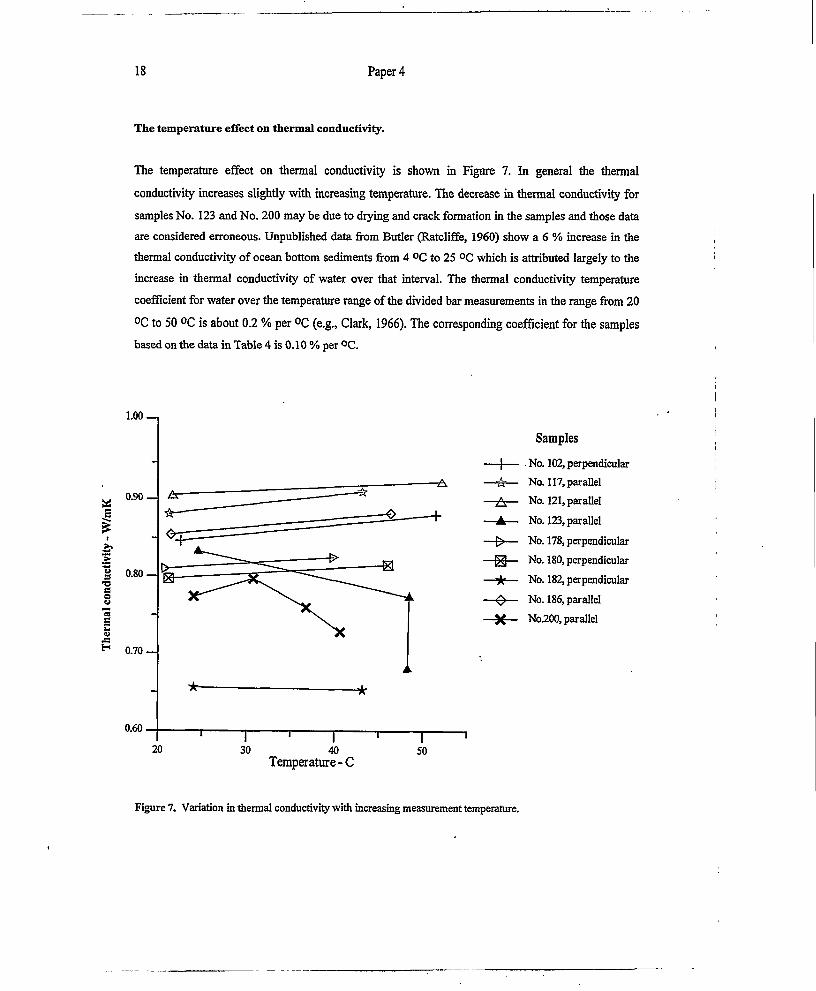
Ther
mal
cond
uctiv
ity -
W/m
K
18 Paper 4
The temperature effect on thermal conductivity.
The temperature effect on thermal conductivity is shown in Figure 7. In general the thermal
conductivity increases slightly with increasing temperature. The decrease in thermal conductivity for
samples No. 123 and No. 200 may be due to drying and crack formation in the samples and those data
are considered erroneous. Unpublished data from Butler (Ratcliffe, 1960) show a 6 % increase in the
thermal conductivity of ocean bottom sediments from 4 °C to 25 °C which is attributed largely to the
increase in thermal conductivity of water over that interval. The thermal conductivity temperature
coefficient for water over the temperature range of the divided bar measurements in the range from 20
°C to 50 °C is about 0.2 % per °C (e.g., Clark, 1966). The corresponding coefficient for the samples
based on the data in Table 4 is 0.10 % per °C.
1.00
0.90— A
0.70 —
Temperature-C
Samples
A■A
*
No. 102, perpendicular No. 117, parallel No. 121, parallel
No. 123, parallel
No. 178, perpendicular No. 180, perpendicular
No. 182, perpendicular No. 186, parallel No.200, parallel
Figure 7. Variation in thermal conductivity with increasing measurement temperature.

Ther
mal
cond
uctiv
ity -
W/m
K
Thermal conductivity of unconsolidated sediments... 19
Comparative measurements.
Thermal conductivities measured by needle probe and divided bar apparatus are shown in Figure 8.
The needle probe represents a combined value of parallel and perpendicular thermal conductivity. In
order to compare the two methods, values of the parallel and perpendicular divided bar measurements
are used to calculate km from Equation 5, which is derived from the basic equation for an ellipse (e.g.
Penner, 1963; Demongodin et al., 1993). Values of km (blue circles, Figure 8) should approximate
needle probe measurements geometry.
km = -JkL -kn (5)
where km - thermal conductivity estimated from the parallel andperpendicular measured divided bar values.
There is a near constant difference between the measured values of thermal conductivity returned by
the two methods. In Figure 8 it can be seen that the needle probe method measures consistently higher
values of thermal conductivity (red squares, Figure 8) for all samples, than those obtained from the
divided bar method, represented by km (blue circles, Figure 8).
Samples
— — Divided bar, perpendicular to thesea bottom.
■ Needle probe
- - * - • Divided bar, parallel to the seabottom.
" • Divided bar, calculated ______ value(km)__________________
!
Figure 8. Comparison of thermal conductivities measured with needle probe and divided bar apparatus. The
needle probe measurements are higher than those measured with the divided bar apparatus.
i

20 Paper 4
Even when a correction for the small sample size in the divided bar measurements is made, the
discrepancy between the two methods of measurements is reduced only by 3.5 % and thus remains
significant. Some difference between the measurements might be expected due to inhomogeneities in
the tested samples since the divided bar measurements were carried out on a part of the needle probe
samples. However, since the difference observed in Figure 8 can be considered as constant (where 7 of
the 10 pairs of measurements differ in the range of 0.13-0.15 W/m-K) random inhomogeneity is not a
likely explanation. The observed difference might, however, be due to:
• calibration error
• errors caused by drying of the samples during storage
• errors caused by the preparation of the samples
• errors caused by environmental conditions during measurements.
Calibration error.
A calibration error is a measurement error related to the instrument and the measurement methodology
expressed as lack of correspondence between the two different methods. This will be a systematic
error. The difference in our results obtained by the two methods is similar to that reported previously
by Slusarchuk & Foulger (1973), Farouki (1981) and Somerton (1992). Their measurements with the
needle probe techniques were in the range of 15 - 20 % higher than those with the divided bar
apparatus. Also previously unpublished measurements carried out at Department of Refrigeration
Engineering, Norwegian University of Science and Technology confirm a methodical discrepancy (H.
Johansen, pers. comm.1996), where a needle probe was inserted in the divided bar samples during the
measurements. The needle probe measured about 20 % higher thermal conductivity than the divided
bar. This result disagrees with the measurements on clayey unconsolidated sediments by Von Herzen
& Maxwell (1959) and consolidated samples by Brigaud & Vasseur (1989) who did not detect any
discrepancy between the two methods. Slusarchuk & Foulger (1973) and Farouki (1981) postulated
that calibration error may explain their measured discrepancy between the two methods. Slusarchuk &
Foulger (1973) and Farouki (1981) considered the values obtained by the divided bar apparatus as the
most correct thermal conductivity value.

Thermal conductivity of unconsolidated sediments... 21
Errors caused by drying of the samples during storage.
As the needle probe measurements were carried out onboard ship just after sampling, while the divided
bar measurements were performed up to 7 months later drying of the samples during storage might be
a reason for the lower values measured with the divided bar apparatus (e.g., Von Herzen & Maxwell,
1959). The considerable lowering of thermal conductivity with increasing temperature for samples No.
123 and No. 200 (Figure 7) is probably due to drying of the samples. If drying was the main reason for
the discrepancy, a random and not as observed a rather constant discrepancy between the methods,
would be expected. The 11 samples have a high water content in the range of 53 - 79 % (Table 4), and
they have been subjected to the same physical conditions in the time between the needle probe and the
divided bar measurements. The divided bar measurement of sample No. 197 at 25 °C and sample 200
at 41 °C were reproduced after respectively 4 and 8 days. The samples were stored in the divided bar
apparatus. Exactly the same thermal conductivity values were obtained for both of the samples. For
sample No. 123 a decrease in the measured thermal conductivity of 7 % and 18% was observed after
lying respectively one and two days in the divided bar apparatus. A small temperature effect is
included in this reduction. From these results and also from experience gained from measurements
carried out on claystones from England (Midttemme et al., 1997a) drying of the samples seems to
cause a pronounced lowering of the thermal conductivity. We would from our experience have
expected this drying effect to be random. On the other hand, because of the character of these samples
we will not exclude that there might be a systematic effect of drying on the divided bar results.
Errors caused by preparation of the samples.
The divided bar apparatus requires a more exact and comprehensive preparation of the samples (Von
Herzen & Maxwell, 1959; Farouki, 1981). This may be a drawback especially for soft sediments.
Compaction, drying and some disturbance of the sample may occur during the preparation process and
influence the measured thermal conductivity. Compaction and disturbance of the samples during
preparation are assumed to increase the thermal conductivity and these effects are also expected to
cause a more random discrepancy in the measurements, and cannot therefore explain the observed
discrepancy in the measured thermal conductivity, (e.g., Von Herzen & Maxwell, 1959). Drying of the
samples will occur during preparing, and this might, as discussed above, have lowered the thermal
conductivity measured with the divided bar apparatus.

22 Paper 4
Errors caused by the environmental conditions.
Temperature is found to influence thermal conductivity of these samples (Figure 7). The divided bar
measurements were carried out at temperatures from 20 - 25 °C while the temperature range of the
needle probe measurements was 10-20 °C. Based on the previous discussion correction for this effect
would serve to increase the difference between the measurements by about 3 % at most. The effect of
pressure is not significant as all measurements were carried out at about normal atmospheric pressure.
Total effect of errors.
The effects of sample size and the differences in ambient temperatures during measurements are seen
to essentially cancel each other.
Von Herzen and Maxwell (1959) emphasize the need for measuring thermal conductivity shortly
after a core is retrieved and point to changes in thermal conductivity of up to 20%, possible in
relatively short times. They did not discuss the possibility of an increase or a decrease in the thermal
conductivity due to this time lag. In view of the unavoidably long time between needle probe and
divided bar measurements in the present study (up to seven months), ample time was available for
such effects to come to play. However, the fact that we observe a constant discrepancy which is
similar to prior reports of a calibration error between the two methods of thermal conductivity
measurement is disquieting. Resolution of this discrepancy is beyond the scope of our measurements
largely due to the previously discussed time factor. The implications of the discrepancy; however, as
well as the numbers of conflicting reports are sufficient to warrant additional work in this area.
However, for the purposes of the present work on modeling sample to sample differences in thermal
conductivity, Figure 8 shows a high degree of sample to sample correlation between the needle probe
and the divided bar measurements. This lends confidence to our thermal conductivities measured by
the needle probe as the basis for the modeling work which follows. There might also be a change in
thermal conductivity due to changes in the samples compressibility because of the removal from its
initial stress-state. This effect is not considered in this study.

Thermal conductivity of unconsolidated sediments... 23
Modeling thermal conductivity.
Thermal conductivity was estimated by the geometric mean model (Equation 1) using the measured
water content values and a constant water conductivity, kw, of 0.60 W/m-K. The matrix conductivity,
kg was calculated: 1) from the mineralogy (Equation 4) by using the Horai (1971) values of mineral
conductivities (Table 1) and 2) by Johansen’s (1975) method (Equation 6), which is based on the
quartz content. ks = • kl~Vr- (6)
where kg2 quartz conductivity, 7.70 W/m-K,k0 thermal conductivity of the other minerals, 2.00 W/m-K,vqz - content of quartz (0.00 - 1.00).
The values calculated were plotted versus measured thermal conductivity values carried out by the
needle probe method (Figure 9). Both models calculated higher values than the measured. Of the two
models Johansen’s model predicts thermal conductivities better than the model based on the total
mineralogy. The mean deviation between estimated and measured values are respectively 0.06 W/m-K
(6 %) and 0.11 W/m-K (12 %). From these results, except for a possible effect of quartz, there seems to
be low correlation between the mineralogy and the measured thermal conductivity for these
unconsolidated, water rich sediments.
In an attempt to develop a better model for the studied sediments, and to test the influence of the
mineral properties, different models of thermal conductivity are proposed and tested. Thermal
conductivities measured by needle probe are taken to give the correct results. The models are predicted
by the geometric mean equation (Equation 1) where thermal conductivity of the water is taken as
constant, kw = 0.60 W/m-K for all models. The models differ as to how the matrix thermal conductivity
(ks) is estimated. Four methods to model matrix conductivity have been tested:
1. ks as a constant
2. kg estimated from the mineralogy
3. ks estimated from the grain size fractions
4. kg estimated from the mineralogy and grain size fractions.
In methods 2, 3 and 4 the matrix conductivity is estimated from the geometric mean equation
(Equation 2). The models were tested by non-linear regression analysis of the geometric mean model,
where the laboratory data of water content, mineralogy and grain size distribution are used as the

Mea
sure
d th
erm
al c
ondu
ctiv
ity -
W/m
K 1.60 —
¥± +
80 1.20 1. Estimated thermal conductivity - W/mK
Nnfca'cfsarrpfes
Figure 9a Thermal conductivities estimated with Johansen’s (1975) method versus values measured with the needle probe. The solid line is the unity line (1:1). The dotted line is the regression line. The deviation between the estimated and measured values are shown in the histogram.
Paper 4

Mea
sure
d th
erm
al co
nduc
tivity
- W
/mK
K
Figure 9b Thermal conductivities estimated with the geometric mean model based on the mineralogy versus values measured with the needle probe. The solid line is the unity line (1:1). The dotted line is the regression line. The deviation between the estimated and measured values are shown in the histogram.
Thermal conductivity of
unconsolidated sediments...

Table 6. Models of matrix thermal conductivity The mineral and grain size conductivities (W/m-K) are found by non-linear regression analyses.(qz = quartz, fsp = feldspar, ca =calcite, dol = dolomite, ka= kaolinite, S/I =smectite and illite, clay = clay minerals, re = remaining minerals, >63=> 63pm fraction, 2-63 = 2pm - 63pm fraction, <2 = < 2 pm fraction). The conductivity of water is kept constant as 0.60 W/nvK.
Model 1 k, constant1. k,=2.45 R2 =0.813Model 2 dependent on mineralogy.2.1 Qz,Fsp,Ca,Dol,Ka,S/I R2 =0.864 k, «= 5.03 kfip=2.97 k„=1.68 kdo1=1.64 kk.=0.08 ks„=3.34 k,c=2.00
2.2 Qz,Fsp,Ca,Ka,S/l R2 =0.864 kqi= 5.03 kr, p=2.94 ke.-l.67 kk=0.08 ky,=3.31 k„=2.722.3 Qu,Fsp,Ca,S/I R2 =0.853 kq = 4.87 kr,p=3.00 kc.=1.30 ksn-2.29 k[c—0.702.4 Qz, Fsp, S/I R2 =0.852 kqz= 4.71 krsp=2.97 ksn=2.07 k[c=1.062.5 Qz,Fsp,Ca,Dol,Clay R2 =0.850 kqz= 4.20 kr.p-3.08 ke.-l.08 kdol=2.14 ke„=1.48 krc=3.162.6 Qz,Fsp,Ca,Clay R2 =0.850 kq,= 4.20 kftp=3.I0 ke.-l.08 kgi.,-1.49 k,e=2.49
2.7 Qz,Ca,Clay R2 =0.850 kqz=4.17 ke.-l.07 kei,y=1.48 krc=3.032.8 Qz,Fsp,Ca R2 =0.849 kq z= 4.33 kf,p=3.09 ke.-l.10 krc=1.582.9 Fsp,Ca,Clay R2 =0.849 kftp-3.10 ke.-l.06 kc,„=1.43 kre=3.982.10 Ca.Clay R2 =0.848 ke.-l.10 k«i.y=1.35 krc=3.612.11 Qz,Fsp,Clay R2 =0.848 kq.-4.29 krsp= 3.16 kgi.y-l.5I k,c=1.282.12 Qz,Fsp R2 =0.848 kqz=4.I9 kfsp= 3.22 k,e=1.41
2.13 Qz,Ca R2 =0.844 kqz=4.81 k..—0.98 k„=2.142.14 Qz,Clay R2 =0.840 kqz=4.34 kel„=1.51 k[c=2.232.15 Fsp,Ca,S/I R2 =0.840 kr,p=3.09 kg.-0.93 ks/|—1.37 k[c=3.492.16 Qz R2 =0.838 kq,= 4.71 k,c=1.88
2.17 Qz,S/I R2 =0.838 kq.- 4.85 ky.-2.07 krc=1.802.18 Fsp,Clay R2 =0.834 kf,p= 3.61 kclay—1.18 k„=2.842.19 Clay R2 =0.832 kgi.y-1.23 k„=3.072.20 Fsp, S/I R1 =0.825 kr>p=3.56 ksr.-l.21 k,=2.502.21 Fsp.Ca R2 =0.825 kf, p=2.85 ke.-l.00 kre=2.742.22 Ca R2 =0.825 ke„=1.00 k,,=2.782.23 S/I R2 =0.823 ky.-l.30 klc=2.782.24 Fsp R1 =0.816 kr,p=3.28 krc=2.18Model 3 dependent on grain size distribution.3.1 >63,2-63, <2 R2 =0.878 k>63=5.24 k2.63=2.00 k<2=2.263.2 >63 R1 =0.878 k>63=5.19 k<63=2.173.3 <2 R2 =0.860 k,2=4.03 k<2=1.68Model 4 dependent on grain size distribution and mineralogy4 Qz,Fsp,Ca,Ka,S/I,>63, R2 =0.883 kq.-6.82 kr,p= 3.49 k..— 3.62 kk.= 0.06 ky,= 1.61 k„=3.43 k>63=5.46 k2.63=1.80 k^-2.22
2-63,<2 (Xm, =0.238)
Paper 4

Thermal conductivity of unconsolidated sediments... 27
variables. Based on the thermal conductivities measured with the needle probe, the thermal
conductivities of the minerals and grain size fractions were determined by regression analysis. The
analyses were run by the statistical program SPSS 6.1 for Windows. A total of 24 mineralogical
models (Models 2.1 - 2.24) and 3 grain size models (Models 3.1 - 3.3) were tested. Results of the
statistical analysis are presented in Table 6. The coefficient of determination, R2 is the adjusted
coefficient to which corrects for the number of independent variables.
Model 1. ks as a constant.
Model 1 is the simplest model where both thermal conductivities of water, kw and matrix, ks are
considered to be constants. The thermal conductivity is then expressed as a function of the water
content only. The best fit result from the regression analysis (Table 6) was when ks was 2.45 W/m-K.
A coefficient of determination, R2 of 0.813, was then obtained. Model 1 is shown in the scatterplot of
thermal conductivity versus water content (Figure 10). By this simple model where all qualitative
information of the matrix is ignored, thermal conductivity is estimated within a standard error
estimates of 20 %. This result emphasizes the major influence of water content on the thermal
conductivity of these sediments, and clearly demonstrates the decrease in thermal conductivity as the
water content increases. Figure 10 shows best agreement between Model 1 and the measured thermal
conductivities when the water content is in the range of 60 - 75 %. The measured values for the
samples with highest water content are lower than the values predicted with this model. The water
content of these samples are, as mentioned previously probably too low (< 3 %). A small increase in
the water content for these samples would improve the coefficient of determination and the quality of
the model.

28 Paper 4
Model 1. kg is constant.
k = k<1_w) -k”
ks = 2.45 W/m-K kw= 0.60 W/m-K R2 = 0.813
40 60 80 100Water content - % of volume
Figure 10. Scatterplot of water content versus measured thermal conductivity. The line represents the simplest model (Model 1), where ks is constant
Model 2.1
kg modeled from the mineralogy.
R2 = 0.864
0.80 no1 Measured thermal conductivity - W/mK
Figure 11. Values of thermal conductivities obtained by the best mineralogy model (Model 2.1) versus measured
thermal conductivities. Unity relationship (1:1) is shown with solid line. Linear regression is shown with dotted
line.

Thermal conductivity of unconsolidated sediments... 29
Model 2. ks dependent on the mineralogy.
Different mineral dependent models were tested with use of different contents of minerals (Table 6).
The 7 main minerals in the samples; quartz, feldspar, calcite, dolomite, kaolinite, illite and smectite are
used in the modeling. The contents of illite, smectite and mixed layer illite/smectite are combined and
named smectite/illite. The best fit model (Model 2.1) was obtained when the calculation of the matrix
thermal conductivity (ks) was based on all 6 mineral fraction (Figure 11).
= *2= .*%, (?)
whereVi - volume fraction of mineral i,kqZ - thermal conductivity of quartz = 5.03 W/m-K,kfsp - thermal conductivity of feldspar=2.97 W/m-K,kca - thermal conductivity of calcite = 1.68 W/m-K,kdol - thermal conductivity of dolomite =1.64 W/m-K,kb, - thermal conductivity of kaolinite = 0.08 W/m-K,ks/i - thermal conductivity of smectite and illite = 3.34 W/m-K,kre - thermal conductivity of remaining minerals = 2.00 W/m-K
The coefficient of determination, R2 is 0.864 for this model, which is an improvement on the simplest
model (Model 1) by 5.1 %. Some trends are observed from the 24 different mineralogical models
(Models 2.1 - 2.24 in Table 6) and the correlation matrix (Table 7). The coefficients of determination
show that of the 6 mineral fractions, quartz has the greatest, and feldspar and dolomite the least
influence on thermal conductivity. Values of mineral conductivities obtained from the statistical
analysis are given in Table 6. In agreement with the literature values (Table 1) quartz is found to have
the highest mineral conductivity, but the values of mineral conductivity in the mineralogical models
2.1 - 2.24 do in general not correspond with those reported in the literature. A particularly high
deviation is detected for the mineral conductivities of kaolinite and dolomite. A mineral conductivity
of 0.08 W/m-K for kaolinite which is only 7 % of thermal conductivity of water appears unrealistic.
Model 3. ks dependent on grain size distribution.
Three grain size models were tested. The thermal conductivities of the grain size fractions were found
from the best fit results from the regression analyses (Table 6). A coefficient of determination, R2 of
0.878 was obtained by two of the models, respectively when all three fractions (Equation 8) and when
only the coarsest fraction is used (Figure 12) (Equation 9).

30 Paper 4
where
(8)
Vik>63h-63k<2
volume fraction of the grain size fraction i, thermal conductivity of the grain fraction >63 pm = 5.24 W/m-K, thermal conductivity of the grain fraction 2 - 63 pm = 2.00 W/m-K, thermal conductivity of the grain fraction < 2 pm = 2.26 W/m-K.
(9)where &><y - thermal conductivity of the grain fraction >63 pm = 5.19 W/m-K,
k<$3 - thermal conductivity of the grain fraction <63 pm = 2.17 W/m-K.
The high influence of the coarsest grain size fraction (> 63 pm) on the thermal conductivity is
confirmed by the correlation coefficient matrix (Table 7). Next to water content, this fraction has the
highest correlation with the measured thermal conductivity (r = 0.81). Using only the finest grain size
fraction (Model 3.3) a coefficient of determination, R2 = 0.860 is obtained, which is better than the
mineralogical models 2.2 - 2.24, but slightly worse than Model 2.1.
Model 3.2
k$ modeled from the coarsest grain size fractions.
R2= 0.878.
0.80 1.00 120 1.40Measured thermal conductivity - W/mK
Figure 12. Thermal conductivities modeled from the grain size fraction > 63pm (Model 3.2) versus measured
thermal conductivities. Unity relationship (1:1) is shown with solid line. Linear regression is shown with dotted
line.

Thermal conductivity of unconsolidated sediments... 31
Table 7. Correlation matrix of thermal conductivity, water content, grain size and mineralogical characteristics.
Thermalcond
Watercontent > 63/an 2 -63/an <2/an
Thermalconductivity 1 -090 081 -053 -039
Watercontent -090 1 -072 060 022> 63/an 081 -072 1 -049 -0622-63/an -053 060 -0.49 1 -038<2/an -039 022 -062 -038 1Quartz 038 -031 044 -016 -032
Feldspar 010 -008 027 -004 -025Calcite -021 017 -031 025 Q10
Dolomite -001 002 -007 -004 012Kaolinite -035 025 -049 005 049
Illite / smectite -019 013 -028 -009 038
Quartz Feldspar Calcite Dolomite Kaolinite _smectite038 010 -021 -001 -035 -019
-031 -008 017 002 025 013044 027 -031 -007 -049 -028-016 -004 025 -Q04 005 -009-032 -025 010 012 049 038
1 -017 -040 002 -031 -054-017 1 -041 -019 -040 -030-040 -041 1 -007 005 -029002 -019 -007 1 001 -012
-031 -040 005 001 1 044-054 -030 -029 -Q12 044 1
Model 4. ks dependent on the mineralogy and grain size distribution.
The best model is obtained using both the mineralogical and grain size fractions. The matrix
conductivity is estimated from the following equation:
*2" - #)+(i - %)(<%' - *2# - ) do)
where xVikqzkfipkcakhaks/Ikrek>63k2-63k<2
ratio estimated from the mineralogical parameters = 0.24 volume fraction of mineral and grain size fraction i, thermal conductivity of quartz = 6.82 W/m-K, thermal conductivity of feldspar = 3.49 W/m-K, thermal conductivity of calcite = 3.62 W/m-K, thermal conductivity of kaolinite = 0.06 W/m-K, thermal conductivity of smectite and illite = 1.61 W/m-K, thermal conductivity of remaining minerals = 3.43 W/m-K, thermal conductivity of grain size fraction >63 pm = 5.46 W/m-K, thermal conductivity of grain size fraction 2-63 pm = 1.80 W/m-K, thermal conductivity of grain size fraction <2 pm = 2.22 W/m-K.
With a coefficient of determination of 0.883 this model improves the calculation of thermal
conductivity by 7.0 % compared to the simplest model (Model 1). A value of x of 0.24 will mean that
the grain size fractions have three times greater influence on thermal conductivity in this model than
the mineralogy. An improvement of only 7 % of the results by the rather complex Model 4 compared
to the simple Model 1 is lower than expected. This is in view of the fact that heat is mainly transferred
through the solid part of the samples. Though this study is based on samples with low matrix volume
(15-60 %) (Figure 2) and relatively small variations in mineralogy and grain size distribution (Table 3),
the matrix properties were expected to have greater influence on thermal conductivity.

32 Paper 4
Related to the conductivities of the grain size fractions (Table 6) the coarsest fraction (>63 pm) has
considerably higher conductivity than the two other fractions. Noticeable is that the finest fraction (<2
pm) is found to have higher conductivity than the medium fraction (2-63 pm). Compared with the
literature values of mineral conductivity (Table 1) the values obtained by this model (Model 4), with
one exception, are more reasonable than those obtained from the mineralogical models (Models 2.1 -
2.24). In this model the mineralogical conductivities of quartz, calcite and illite/smectite are close to
the values previously reported in the literature. The conductivity of kaolinite still appears
unrealistically low.
Model 4. kj modeled from mineralogy and grain size fractions.
k = k<'-w) •k
ks =x(kq> -kf> kc> -kk> -ksv//' -krve") + (l-
x = 0.24, kqZ = 6.82, kfsp = 3.49, k^ = 3.62, kka = 0.06, kS/i = 1 k>63 = 5.46, k2-63 = 1.80, k<2 = 2.22 R2= 0.883.
x)(k>6f ’k 2-6*1
,61,kre = 3.43,
0.80-
Measured thermal conductivity - W/mK
Figure 13. Thermal conductivities for the “best fit” model (Model 4) versus measured thermal conductivities.
Unity relationship (1:1) is shown with solid line. Linear regression is shown with dotted line.
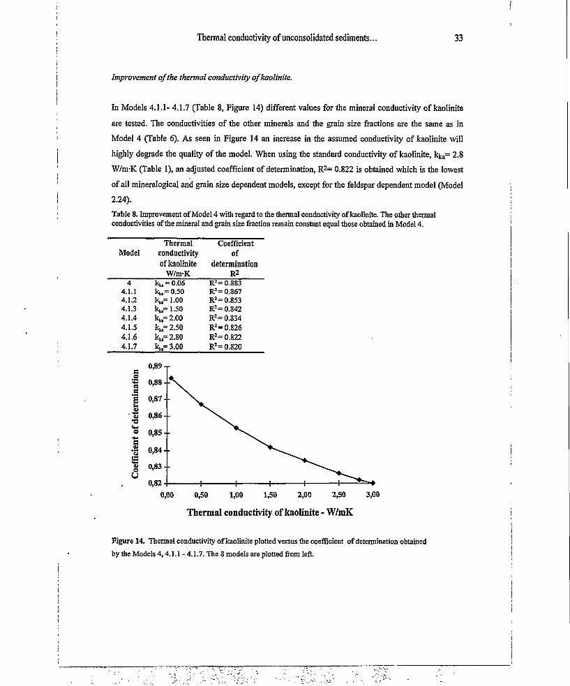
Thermal conductivity of unconsolidated sediments... 33
Improvement of the thermal conductivity ofkaolinite.
In Models 4.1.1- 4.1.7 (Table 8, Figure 14) different values for the mineral conductivity ofkaolinite
are tested. The conductivities of the other minerals and the grain size fractions are the same as in
Model 4 (Table 6). As seen in Figure 14 an increase in the assumed conductivity of kaolinite will
highly degrade the quality of the model. When using the standard conductivity ofkaolinite, k%a= 2.8
W/mrK (Table 1), an adjusted coefficient of determination, R2= 0.822 is obtained which is the lowest
of all mineralogical and grain size dependent models, except for the feldspar dependent model (Model
2.24).
Table 8. Improvement of Model 4 with regard to the thermal conductivity ofkaolinite. The other thermal conductivities of the mineral and grain size fraction remain constant equal those obtained in Model 4.
ModelThermal
conductivityofkaolinite
W/m-K
Coefficientof
determinationR2
4 kb = 0.06 R2= 0.8834.1.1 kb= 0.50 R2= 0.8674.1.2 kb= 1.00 R2= 0.8534.1.3 kb= 1.50 R2= 0.8424.1.4 kb= 2.00 R2= 0.8344.1.5 kb= 2.50 R2= 0.8264.1.6 kfc = 2.80 R2= 0.8224.1.7 kb= 3.00 R2= 0.820
0,89-r
0,88 - -
0,86--
0,83 - -
Thermal conductivity ofkaolinite - W/mK
Figure 14. Thermal conductivity ofkaolinite plotted versus the coefficient of determination obtained
by the Models 4,4.1.1 - 4.1.7. The 8 models are plotted from left

34 Paper 4
Since thermal conductivities of grain size fractions have not been previously published, it is difficult to
confirm the values obtained in Model 4. In models 4.2.1-4.2.7 (Table 9, Figure 15) the conductivity of
kaolinite has also been adjusted. The conductivities of the grain size fractions are allowed to vary, and
the best fit models are determined by non-linear regression analysis. The other mineral conductivities
remain constant. For these models only a slight worsening in the coefficient of determination is
obtained when increasing the conductivity of kaolinite. The increase in kaolinite conductivity is
accompanied by a decrease in the conductivity of < 2 pm and 2-63 pm fractions and an increase in the
>63 pm fraction (Figure 15). We have no explanation of these results.
Table 9. Improvement of Model 4 with regard to the thermal conductivity of kaolinite. The other mineral conductivities remain constant equal those in Model 4. The grain size conductivities are allowed to vary. The best fit models are determined by non-linear regression analysis.
ModelThermal
conductivity of kaolinite
W/m-K
Thermalconductivity
of>63pmfractionW/m-K
Thermalconductivityof2-63pmfractionW/m-K
Thermal conductivity
of < 2pm fraction W/m-K
Coefficientof
determinationR2
4 Iq, = 0.06 k^3= 5.46 ^2-63= 1*80 2.22 R2= 0.883
4.2.1 kt,= 0.50 k>o= 5.57 k2^3= 1.65 k<2= 2.05 R2= 0.883
4.2.2 kb= 1.00 k»o= 5.64 kM3= 1.60 k<2= 1.99 R2= 0.883
4.2.3 kh= 1.50 k>o= 5.69 k2^3= 157 k<,= 1.95 R2= 0.883
4.2.4 k% = 2.00 k>6,= 5.74 kw]= 1.54 kQ= 1.92 R2= 0.883
4.2.5 1^= 2.50 k*;3= 5.77 k2«= 1.53 k^= 1.90 R2= 0.882
4.2.6 1^,= 2.80 k>63= 5.79 kM3= 1.52 ka= 1.89 R2= 0.882
4.2.7 kfc,= 3.00 k><a= 5.80 kM3= 1.51 k<2= 1.88 R2= 0.882
5,00 - -
4,00 - -
3,00--
2,00 - -
1,00 - -
Models
-kaolinite ->63 fraction -2-63 fraction
—X—<2 fraction
Figure 15. Variation in the conductivity of kaolinite, >63 pm fraction, 2-63pm fraction and <2 pm fraction.
(Models 4.2.1 - 4.2.7).

Thermal conductivity of unconsolidated sediments... 35
For these unconsolidated sediments the most reasonable model proposed, related to previously
published mineral conductivities (e.g. Horai, 1971; Brigaud & Vasseur, 1989) and the coefficient of
determination obtained, seems to be Model 4.2.6 (Equation 9). The adjusted coefficient of
determination, R2 is 0.882.
where ratio estimated from the mineralogical parameters = 0.24 volume fraction of mineral and grain size fraction i, thermal conductivity of quartz=6.82 W/m-K, thermal conductivity of feldspar=3.49 W/m-K, thermal conductivity of calcite = 3.62 W/m-K,. thermal conductivity of kaolinite = 2.80 W/m-K,. thermal conductivity of smectite and illite =1.61 W/m-K, thermal conductivity of remaining minerals1 - 3.43 W/m-K, thermal conductivity of grain size fraction >63 pm = 5.79 W/m-K, thermal conductivity of grain size fraction 2-63 pm = 1.52 W/m-K, thermal conductivity of grain size fraction <2 pm = 1.89 W/m-K.
xVikqzkfipkcakkaks/lkrek>63k2-63k<2
CONCLUSION.
Thermal conductivities of unconsolidated sediments from the Voting Basin, measured with a needle
probe, range from 0.69 - 1.57 W/m-K. Comparative measurements of thermal conductivity with
divided bar apparatus give lower thermal conductivity values. The difference between the
measurements seems to be rather constant. The possibility that the difference may be due to systematic
calibration error between the two methods, warrants further investigation.
A model which estimates thermal conductivity for unconsolidated sediments with a coefficient of
determination, R2 of 0.88 is developed. For these unconsolidated sediments water content is found to
have the major influence on thermal conductivity, and a fairly good estimate of thermal conductivity
can thus be made directly from the measurements of water content (R2 =0.81). Grain size fractions, and
especially the content of the coarsest fraction (> 63 pm) strongly influence thermal conductivity, and is
for these sediments a more important factor than the total mineralogy. Thus the model based on water
content, grain size fractions and mineralogy was found to be the best, a simpler model based on the
content of coarsest fraction (> 63 pm) and water content is suggested to be the preferable model for the
thermal conductivity of these unconsolidated sediments.

36 Paper 4
ACKNOWLEDGEMENTS.
This work has been financially supported by Norwegian Research Council Grant (NFR) 440.91/046
and Statoil. We are grateful to Helge Johansen, Department of Refrigeration, Norwegian University of
Science and Technology (NTNU) for the divided bar measurements, the Geotechnical Department,
NTNU for kind assistance with the measurements of water content and Professor Stephen Lippard,
Department of Geology and Mineral Resources Engineering, NTNU for improving the English
language of the manuscript.
REFERENCES.
Anand, J., W.H. Somerton, & E. Gomaa, 1973, Predicting thermal conductivities of formations from other known properties. Society of Petroleum Engineers Journal, p. 267-273.
Balling, N., J.I. Kristiansen, N. Breiner,K.D. Poulsen, R. Rasmussen & S. Saxov, 1981, Geothermalmeasurements and subsurface temperature modelling in Denmark. Geoskrifter, no. 16, Department of Geology, Aarhus University, 172 p.
Beck, A.E, 1988, Methods for determining thermal conductivity and thermal diffusivity, in R. Haenel, L.Rybach, and L. Stegena, eds., Handbook of terrestrial heat-flow density determination: Dordrecht, Kluwer, p. 87-124.
Birch, F. & H. Clark, 1940, The thermal conductivity of rocks. American Journal of Science, 238, 8, p. 529-558.
Blackwell, D.D. & J.L. Steele, 1989, Thermal conductivity of sedimentary rocks: measurements andsignificance, in N.D. Naeser & T.H. McCulloh, eds., Thermal history of sedimentary basins, methods and case histories, Springer Verlag, New York, p. 13-36.
Blystad, P., H. Brekke, R.B. Fzerseth, B.T. Larsen, J. Skogseid, B. Temdbakken, 1995, Structural elements of the Norwegian continental shelf. Part II: The Norwegian Sea Region. NPD-Bulletin No. 8. The Norwegian Petroleum Directorate 45 p.
Brendeng, E. & P.E. Frivik, 1974, New developement in design of equipment for measuring thermalconductivity and heat flow. Heat transmission measurements in thermal insulations, ASTM STP 544, American Society for Testing and Materials, p. 147-166.
Brigand, F. & G. Vasseur, 1989, Mineralogy, porosity and fluid control on thermal conductivity of sedimentary rocks, Geophysical Journal, v. 98, p. 525-542.
Brigaud, F., D.S. Chapman & S. Le Douaran, 1990, Estimating thermal conductivity in sedimentary basins using lithological data and geophysical well logs, AAPG Bulletin, v. 74, p. 1459-1477.
Brindley, G.W. & G. Brown, 1980, Crystal structures of clay minerals and their X-ray identification,Monograph, no. 5, Mineralogical Society, London, 495 p.
Clark, S.P. jr., 1966, Handbook of physical constants, The Geological Society of America, Inc.Memoir 97, 587 p.
Demongodin, L., B. Pinoteau, G. Vasseur & R. Gable, 1991, Thermal conductivity and well logs: a case study in the Paris basin, Geophysical Journal International., v. 105, p. 675-691.
Demongodin, L., G. Vasseur & F. Brigaud, 1993, Anisotropy of thermal conductivity in clayey formations, in A.G. Dore, J.H. Auguston, C. Hermanrud, D.S. Stewart & 0. Sylta, eds., Basin modelling: advances and applications, Norwegian Petroleum Society (NPF) Special Publication 3, Elsevier, Amsterdam, p. 209-217.
Eldholm, O., J. Thiede, E. Taylor, et aL, 1987, Proceedings of the Ocean Drilling Program, part A - Initial Reports, v. 104, College Station, TX, 783p.

Thermal conductivity of unconsolidated sediments... 37
Eldholm, 0., J. Thiede, E. Taylor, et al., 1989, Proceedings of the Ocean Drilling Program, Scientific Results v. 104 College Station, TX, 1141 p.
Farouki, O.T., 1981, Thermal properties of soils, Cold Regions Research and Engineering Laboratory (CRREL) Monograph 81-1, Hanover, New Hampshire, 151p.
Farouki, O.T., 1982, Evalution of methods for calculating soil thermal conductivity, Cold RegionsResearch and Engineering Laboratory (CRREL) Report 82-8, Hanover, New Hampshire, 89p.
Fjeldskaar, W., E. Prestholm, G. Guargena & M. Stephenson, 1993, Mineralogical and diagenetic control on the thermal conductivity of the sedimentary sequences in the Bjornoya Basin, Barents Sea in A.G. Dore, J.H. Auguston, C. Hermanrud, D.S. Stewart & 0. Sylta, eds., Basin modelling: advances and applications, Norwegian Petroleum Society (NPF) Special Publication 3, Elsevier, Amsterdam, p. 445-453.
Folk,R., 1954, The distinction between grain size and mineral composition in sedimentary-rock nomenclature.The Journal of Geology, 62 p. 344-359.
Gilliam, T.M. & I.L. Morgan, 1987, Shale: measurement of thermal properties, Oak Ridge National Laboratory ORNL /TM-10499, Oak Ridge, Tennessee, 138 p.
Goldsmid, H.J. & A.E. Bowley, 1960, Thermal conduction in mica along the planes of cleavage, Nature, v.187, p. 864-865.
Griffiths, C.M..N.R. Brereton, R. Beausillon & D. Castillo, 1992, Thermal conductivity prediction from petrophysical data: a case study, in A. Hurst, C.M. Griffiths, P.F. Worthington, eds, Geological Applications of Wireline Logs II, Geological Society Special Publication, No. 65, p.299-315.
Hermanrud, C., 1993, Basin modelling techniques - an overview, in A.G. Dore, J.H. Auguston, C. Hermanrud, D.S. Stewart & 0. Sylta, eds., Basin modelling: advances and applications, Norwegian Petroleum Society (NPF) Special Publication 3, Elsevier, Amsterdam, p. 1-34.
Horai, K.I., 1971, Thermal conductivity of rock-forming minerals. Journal of Geophysical Research, v. 76, p. 1278-1308.
Horai, K.I. & R.P. Von Herzen, 1985, Measurement of heat flow on leg 86 of the deep sea drilling project. Reprinted from G.R. Heath, L.H. Burckle et al., Initial Reports of the Deep Sea Drilling Prosject, Washington, v. 86, p. 759-775.
Jensen, R.P. & A.G. Dore, 1993, A recent Norwegian Shelf heating event - fact or fantasy ? in A.G. Dore, J.H. Auguston, C. Hermanrud, D.S. Stewart & 0. Sylta, eds., Basin modelling: advances and applications, Norwegian Petroleum Society (NPF) Special Publication 3, Elsevier, Amsterdam, p 85-106.
Jessop, A.M, 1990, Thermal Geophysics. Elsevier, 306 p.Johansen, 0., 1975, Varmeledningevne av jordarter. Dr.ing avhandling, institutt for kjaleteknikk, Norwegian
Institute of Technology (NTH), Trondheim, 23 Ip, (Thermal conductivity of soils. Ph.D. thesis, Cold Region Research and Engineering Laboratory (CRREL) Draft Translation 637, 1977, ADA 044002,Hanover, New Hampshire.
Kasameyer, P.K., R.P. Von Herzen & G. Simmons, 1972, Layers of high thermal conductivity in the north Atlantic, Journal of Geophysical Research, v. 77, p. 3162-3167.
Matsuda, Jun-Ichi & R.P. Von Herzen, 1986, Thermal conductivity variation in a deep-sea sediment core and its relation to H20, Ca and Si content, Deep-Sea Research, v. 33, p. 165-175.
McKenna, T. E., J. M. Sharp, Jr., and F.L. Lynch, 1996, Thermal conductivity of Wilcox and Frio sandstones in south Texas (Gulf of Mexico Basin), AAPG Bulletin, v. 80, p. 1203-1215.
Middleton, M., 1994, Determination of matrix thermal conductivity from dry drill cuttings, AAPG Bulletin v. 78, p. 1790 -1799.
Midttemme, K., E. Roaldset & P. Aagaard, 1994, Termiske egenskaper i sedimentasre bergarter, Rapport fra institutt for geologi og bergteknikk, Norwegian University of Technology (NTH), nr. 29,94 p.
Midttemme, K. & E. Roaldset, 1997, The influence of clay minerals on thermal conductivity of sedimentary rocks, Extended abstract, Nordic Society for Clay Research, meddelande nr. 11
Midttemme, K., E. Roaldset & P. Aagaard, 1997a, Thermal conductivity of selected clay- and mudstones from England, Clay Minerals, 33,131-145.
Midttemme, K., E. Roaldset, & P. Aagaard, 1997b, Thermal conductivity of argillaceous sediments, in. D.M.McCann, M. Eddleston, P. Penning & G.M. Reeves eds., Modem geophysics in engineering geology. Geological Society Engineering Geology Special Publication No. 12, p.355-363.
Midttemme, K. & E. Roaldset, (in press) Thermal conductivity of sedimentary rocks - uncertainties in measuring

38 Paper 4
and modelling. Submitted to Mudrocks at the Basin Scale: Properties, Controls and Behaviour. Geological Society Special Publications
Morin, R. & A.J. Silva, 1984, The effects of high pressure and high temperature on some physical properties of ocean sediments, Journal of Geophysical Research, v. 89-B1, p. 511-526.
Penner, E., 1963, Anisotropic thermal conduction in clay sediments. Proceedings, International Clay Conference, Stockholm, Pergamon Press, Elmsford, v. 1, p. 365-376.
Prestholm, E. & W. Fjeldskaar, 1993, Thermal conductivity anisotropy in sedimentary rocks, and it'sbearing on basin temperature predictions, EUG 7, Strasbourg, France, abstract supplement no. 1 to Terra Nova, v. 5, p. 655.
Pribnow, D. & T. Umsonst, 1993, Estimation of thermal conductivity from the mineral composition:Influence of fabric and anisotropy. Geophysical Research letters, v. 20, p. 2199-2202.
Ratcliffe, E.H. 1960, The thermal conductivities of ocean sediments, Journal of Geophysical Research 65,5, p. 1535-1541.
Robertson, E.C., 1979, Thermal conductivity of rocks, U.S. Geology Survey, Open File Report 79-356,3Op.Rundberg, Y., 1991, Tertiary sedimentary history and basin evolution of the Norwegian North Sea between
60°- 62° N an integrated approach, dr. ing thesis, Department of Geology and Mineral Resources Engineering, Norwegian Institute of Technology, rep.25, Trondheim, 291 p.
Sass, J.H., A.H. Lachenbruch & R.J. Munroe, 1971, Thermal conductivity of rocks from measurements on fragments and its applicatio to heat-flow determinations, Journal of Geophysical Research, v. 76, p. 3391-3401.
SchSn. J.H., 1996, Physical properties of rocks: fundamentals and principles of petrophysics. Seismic exploration, v. 18, Elsevier Science ltd., Oxford, 583 p.
Slusarchuk, W.A. & P.H. Foulger, 1973, Develoment and calibration of a thermal conductivity probeapparatus for use in the field and laboratory, National Research Council of Canada, Div. of BuildingResearch, Technical Paper no. 388, 17p.
Somerton, W.H., 1992, Thermal properties and temperature related behavior of rock/fluid systems. Developements in Petroleum Sciences 37, Elsevier, Amsterdam, 257p.
Vacquier, V., Y. Mathieu, E. Legendre, & E. Blondin, 1988, Experiment on estimating thermal conductivity of sedimentary rocks from oil well logging, AAPG Bulletin, v. 72, p. 758-764.
Vik, E. & C. Hermanrud, 1993, Transient thermal effects of rapid subsidence in the Haltenbanken area. in A.G. Dore, J.H. Auguston, C. Hermanrud, D.S. Stewart & 0. Sylta, eds., Basin modelling: advances and applications, Norwegian Petroleum Society (NPF) Special Publication 3, Elsevier, Amsterdam, p. 107-117.
Von Herzen, R.P & A.E. Maxwell, 1959, The measurements of thermal conductivity of deep sea sediments by a needle probe method, Journal of Geophysical Research, v. 64, p. 1557-1563.
Woodside, W. & J.H. Messmer, 1961, Thermal conductivity of porous media, Journal of Applied Physics, v. 32, p. 1688-1706.
Zimmerman, R. W., 1989, Thermal conductivity of fluid-saturated rocks, Journal of Petroleum Science and Engineering, v. 3, p. 219-227.

Paper 5

Paper 5
The effect of grain size on thermal conductivity of quartz sands and silts*.
Kirsti Midttemme & Elen Roaldset
Department of Geology and Mineral Resources Engineering, Norwegian University of Science and Technology (NTNU),
7034 Trondheim, Norway.
ABSTRACT
Synthetically samples of different grain size fractions of quartz were prepared and the thermal
conductivities measured with a divided bar apparatus. The measurements were earned out on dried
and water saturated samples both perpendicular and parallel to the main stress direction during compaction of the samples. A clear correlation was observed between the porosity and the measured thermal conductivities. For water saturated samples the thermal conductivity decreases
more with increasing porosity than for ideal isotropic material as predicted by the geometric mean
model. A clear positive correlation was also found between the thermal conductivity and the grain
sizes of the samples. When the expected effect of porosity on the thermal conductivity was
excluded, a linear correlation between the logarithm of the grain size and the measured thermal
conductivities of the water saturated samples was found. An anisotropy effect (a = kn/kj in thermal
conductivity was observed for the samples, being most prominent for the coarsest ones. The
measured anisotropy is assumed to be mainly due to the thermal anisotropic nature of the quartz
crystal.
KEYWORDS: thermal conductivity, grain size, quartz samples,
* In press. Petroleum Geoscience.

2 Paper 5
INTRODUCTION.
The three main factors influencing the thermal conductivity of sedimentary rocks are porosity,
mineralogy and texture (e.g. Farouki 1981; Brigaud & Vasseur 1989; Midttomme et al. 1994). Of
these factors, texture is the most difficult to take into account since it is the most complex. The
grain size and the grain size distribution are important factors controlling the texture of sedimentary
rocks. These factors are assumed to influence the thermal conductivity (Anand et al. 1971;
Rzhevsky & Novik 1971; Brigaud et al. 1990; Beziat et al., 1992; Griffiths et al. 1992; Jones &
Pascal 1994; McKenna et al. 1996; Midttomme et al. 1997, 1998 ). Rzhevsky & Novik (1971)
found a decrease in thermal conductivity with decreasing grain size of the material. Their
measurements on quartz samples gave thermal conductivities in the range of 7.0 - 11.7 W/m-K for
monocrystalline, 3.6 W/m-K for polyciystalline samples and 1.39 W/m-K for fused quartz samples
A similar trend was observed for marble and halite. These authors suggested a relationship between
thermal conductivity and average grain size for certain rocks as follows:
where k0 - thermal conductivity of a monocrystal,d„ - mean grain size (mm),B - ratio of the temperature gradient at a grain contact to
the mean temperature gradient of the specimen as a
whole (for marble B«0.027 at 0 °C).
Thermal conductivities estimated by Equation 1 are plotted against the mean grain size in Figure 1.
dav mm
Figure 1. A curve estimated for marble from Equation 1, showing the dependence of thermal conductivity upon grain size d„- mean grain size, k- thermal conductivity, k0 - thermal conductivity of a monocrystal.

The effect of grain size on thermal conductivity of quartz sands and silts. 3
Figure 1 shows that the effect of grain size is most significant for fine-grained material. In a study
of unconsolidated fine-grained sediments, the > 63pm content was, excepting the water content,
found to have greatest influence on the measured thermal conductivities (Midttemme et al. 1997).
The dependence of grain size on thermal conductivity is assumed to be related to the number of
grain contacts per unit path of heat flow (McGaw 1969; Rzhevsky & Novik 1971; Beziat et al.,
1992; Griffiths et al. 1992). The grain contact zones offer more resistance to the heat flow than the
grains itself. This resistance, known as thermal contact resistance (Incropera & De Witt, 1990)
leads therefore to a reduction in thermal conductivity with a decrease in the grain size of the
material. McGaw (1969) and Griffiths et al. (1992) explained the reduction in heat flow caused by
the increased number of grain contacts by thin fluid films between the grains.
Typical values of thermal conductivities measured at 20 °C for clay- and siltstones are 0.80 -1.25
W/m-K, and for sandstones 2.50 - 4.20 W/m-K (Blackwell & Steele 1989). Thermal conductivity
values published by Clark (1966) vary in the range of 0.9 - 6.5 W/m-K for sandstones and 0.6 - 4.0
W/m-K for claystones. By modelling thermal conductivities from well log data from the Paris
Basin, Demongodin et al. (1991) obtained a best fit model by using a matrix conductivity of 6.6
W/m-K for a sandstone matrix and 1.5 W/m-K for a clay matrix. Though these values show a
correlation between the thermal conductivity and the grain size of sedimentary rocks, they can not
be considered as confirmation of a grain size effect on the thermal conductivity, since the grain size
will influence other factors such as porosity, permeability, mineralogy and specific surface area,
which also will influence the thermal conductivity (Figure 2). fit this case the influence of the grain
size can be considered as a secondary effect, which will probably best be taken into account when
considering the primary controlling factors.
Porosity MineralogyPermeabilitySpecificsurface
area
Grain sizes
THERMALCONDUCTIVITY
Figure 2. Flow diagram showing the primary and secondary effects of grain size on thermal conductivity.

4 Paper 5
Porosity is an important factor controlling thermal conductivity (e.g. Brigand & Vasseur 1989;
Griffiths et al. 1992). Pore fluids have a lower thermal conductivity than the matrix in sedimentary
rocks. An increase in porosity will therefore lead to a decrease in the conductivity. At very shallow
depths fine-grained have higher porosities than coarser grained sediments (North 1990), and for
this reason lower thermal conductivities. At depths below 1.5 - 2.0 km sands and sandstones
normally have higher porosities than shales (e.g. Rieke & Chilingarian 1974). The effect of grain
size on porosity will be highest for unconsolidated sediments, since burial history and depth will
greatly influence the porosity for consolidated sediments.
Mineralogy is as the grain size related to sedimentary facies. There will in general be a significant
correlation between the mineralogy and the grain size. Most sandstones contain large amounts of
quartz, which has a high thermal conductivity (k,5BU= 7.7 W/m-K). A high content of clay mineral
is a characteristic property of claystones. The clay minerals have low mineral conductivities (k^ =
1.9 W/m-K, k,__1.9 W/m-K and k^ail= 2.6 W/m-K (values from Brigaud & Vasseur (1989)).
The higher thermal conductivities observed for sandstones than for claystones, may thus be
explained from the mineralogy alone.
Mineralogically based models have been developed, where matrix conductivities are predicted
from the mineralogical composition (Horai 1971; Johansen 1975; Brigaud & Vasseur 1989;
Middleton, 1994; McKenna et al. 1996). Most of these studies have been carried out on sandstones.
McKenna et al. (1996) restricted their study to clean sandstone samples, because of the lack of
mudrock cores and the uncertainties related to the thermal conductivities of clay minerals. Brigaud
& Vasseur (1989) found it impossible to make measurements on clay cores because of the practical
problems related to the coring and sample preparation. They therefore prepared artificial samples
to find the mineral conductivities of the clay minerals. In the studies by Pribnow & Umsonst
(1993) and Midttemme et al. (1997, 1998) on fine-grained materials the mineralogical models
estimate higher thermal conductivities than the measured values (Figure 3). Beziat et al. (1988)
concluded that the mineralogical composition was less important in modelling thermal
conductivities of clays compared to water content (i.e. porosity) and density.
The specific surface area is another factor which is strongly related to the grain size of the
material. It might be difficult to distinguish between the influence of these two factors on the
thermal conductivity. Johansen (1975) considered the grain size distribution of the material as a
secondary factor to the specific surface area in controlling the thermal conductivity. The surface
area effect was explained by the heat flow barrier arising from the water film coating the water wet
mineral grains.

The effect of grain size on thermal conductivity of quartz sands and silts. 5
1.20 1.60Estimated thermal conductivity - W/mK
Samples
London Clay
Fullers Earth
KimmeridgeClay
Oxford Clay
Figure 3. An example of lack of correlation between thermal conductivities estimated by a mineralogically based model and measured values. The solid line is the unity line (1:1). The dotted line is the regression line. The samples are mudstones from England (Midttemme etal. 1998).
Compared to most other minerals, clay minerals have an exceptionally large surface area caused by
both large external and internal surface areas. The effect of the internal surface area on the thermal
conductivity remains unclear, but is assumed to have little effect from the fact that smectite with
extremely high internal surface area of 750 m2/g (van Olphen & Fripiat 1979) has similar mineral
conductivity as illite, with an internal surface area of 5 -10 mYg. For clayey samples, the specific
surface area certainly reflect the content of clay minerals. On the other hand, the content of clay
minerals is strongly related to the grain size, since the finest fractions have the highest contents of
clay minerals.
The grain size will also influence the sizes, shapes and distribution of the pores. The micro
porosity of the most fine grained material will transfer heat differently than a more coarse grained
system (Johansen 1975). The pore size distribution and pore interconnectedness determines the
permeability of the material. The permeability as expressed by Kozeny’s equation is as follows
(e.g. North 1990):
where k - permeability,<J> - porosity,K - Kozeny’s constant,S - specific surface area.
(2)

6 Paper 5
Empirical thermal conductivity models have been developed with permeability as a variable
(Zierfuss & van der Vliet 1956; Anand et al. 1973). By multiple regression analysis Anand et al.
(1973) found a positive correlation between permeability and thermal conductivity of sandstones.
They suggested that this correlation reflected the effect of grain size, since not only permeability
but also thermal conductivity increased with increasing grain size of the material. Later Farouki
(1981) concluded that the effect of permeability on thermal conductivity was related to the specific
surface area.
Even the shape of the grains will influence the thermal conductivity of the material (Johansen
1975; Farouki 1981; Brigaud & Vasseur 1989; McKenna et al. 1996). Thermal conductivities
measured on dry samples of crushed rocks have been found to be considerably higher than on sand
of similar mineralogical composition (Kersten 1949, ref. in Farouki 1981). On the basis of
empirical studies, Johansen (1975) proposed two equations for estimating thermal conductivity
from dry density, one for natural sands and one for crushed rock. At the same dry density the
crushed rock samples gave the highest thermal conductivity.
Anisotropy of thermal conductivity.
A further point of uncertainty in determination of thermal conductivity is the anisotropy effect.
Thermal conductivities measured parallel (k») to the layering are in general higher than those
measured perpendicular (kj. The anisotropy ratio is defined as:
The anisotropy of thermal conductivity correlates with the structural-textural properties of
sedimentary rocks and the orientation of the minerals. Sand and limestones usually show only a
small anisotropy (a < 1.3). The most anisotropic rocks are shales and claystones (a < 4.0) (Schon
1996). Schon (1996) proposed three causes for the anisotropy:
1. crystal anisotropy of the individual rock forming minerals,
2. intrinsic or structural anisotropy resulting from the mineral shapes and their textural
arrangement,
3. orientation and geometry of cracks, fractures and other defects.
Measurements of the anisotropy of minerals published by Cermak and Rybach (1982) show highest
anisotropy for the sheet silicates. The anisotropy of muscovite was 6.1 (k= 0.84 W/m-K, k,,= 5.1
W/m-K). A considerable anisotropy was also measured for quartz (a =1.74, kj. = 6.5 W/m-K, Iq, =
11.3 W/m-K). When the grains are randomly oriented in the matrix, the effect of mineral
anisotropy has little effect on the anisotropy of the thermal conductivity of the rock, but when the
minerals show a preferential orientation the thermal conductivity becomes anisotropic
(Demongodin et al. 1993).

The effect of grain size on thermal conductivity of quartz sands and silts. 7
Modelling the thermal conductivity.
Different models of thermal conductivity have been developed (Farouki 1981; Somerton 1992;
Midttemme et al. 1994; Schon 1996). One of the most successful models is the geometric mean
model. This model is among others used by Brigaud & Vasseur (1989); Middleton (1994) and
McKenna et al. (1996). This simple model is in many cases found to be better than more
sophisticated models used to calculate the thermal conductivity of sediments (Demongodin et al.
1991). The basic geometric mean equation applied to sedimentary rocks is:
(4)
where kK&4
thermal conductivity of sample, W/m-K, thermal conductivity of matrix, W/m-K, thermal conductivity of fluid, W/m-K, porosity (0.00 - 1.00).
Two other basic models, the arithmetic and harmonic mean models, are also widely used
(Somerton 1992; Pribnow & Umsonst 1993; McKenna et al. 1996). These models are based
respectively on parallel and series arrangement of the components relative to the direction of heat
flow. The values estimated by these models give boundary values of thermal conductivity of the
material. For more isotropic samples the geometric mean model would theoretically be most
correct (Midttemme & Roaldset, 1998).
MATERIAL AND METHODS.
Sample preparation.
Synthetically quartz silt- and sandstone samples were prepared from Vatne quartz, a hydrothermal
quartzite with a purity above 99.9 % quartz from Vatne in northern Norway. The material was
crushed and separated into different size fractions by sieving and sedimentation. The grains are
characterized by an elongated and angular form (Figure 4). The synthetic rock samples were
prepared according to the method in Holt & Kenter (1992) and Holt et al. (1993). The different
fractions were mixed with a sodium silicate solution (Na,Si,0,) with compositions varying from 16
g quartz/ml Na-Si-solution for the coarsest to 8.3 g quartz/ml for the finest fractions. The material was
packed in a cylindrical form (d = 4.2 cm), then compacted in a triaxial cell at uniaxial stress
conditions of 10 ton (4.2 MPa) for 5 minutes before hardening by standing for 6 minutes in an
atmosphere of C02. The synthetic rocks were then cut into 3.0 cm cubes (Figure 5). Two samples
of Ottawa sand, a rounded quartzidc beach sand, were prepared by the same method, and included
in this study.
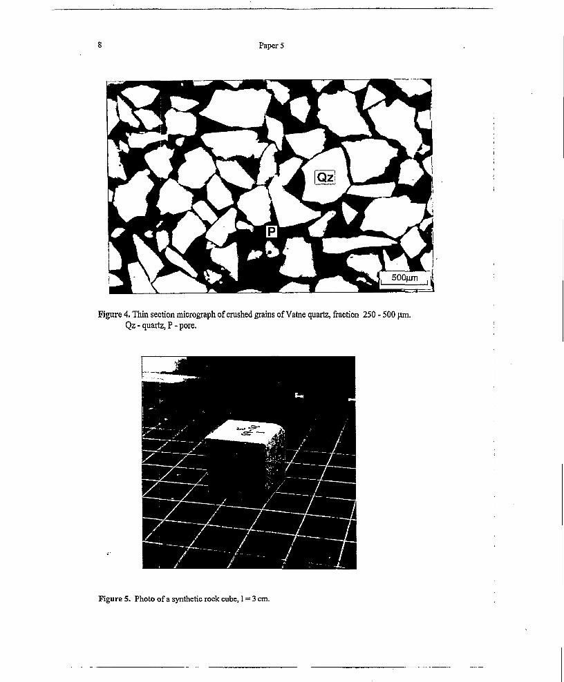
8 Paper 5
Figure 4. Thin section micrograph of crushed grains of Vatne quartz, fraction 250 - 500 pm. Qz - quartz, P - pore.
Figure 5. Photo of a synthetic rock cube, 1 = 3 cm.

The effect of grain size on thermal conductivity of quartz sands and silts. 9
Measurements of thermal conductivities.
Thermal conductivities were measured with a divided bar apparatus, developed at the Institute of
Refrigeration, Norwegian University of Science and Technology (Brendeng & Frivik 1974). This
apparatus was originally designed for bigger samples. Test measurements on samples of different
sizes have shown the measured values to be up to 3.5% lower for cubes of this size (1 = 3.0 cm)
than for the larger ones (1 = 40.0 cm, h = 10.0 cm) (H. Johansen, unpublished 1992). Repeated
measurements on the massive quartzite (sample B) gave an experimental error within 2.5 %. The
synthetic quartz cubes were measured in both water saturated and dried samples, both
perpendicular and parallel to the main stress direction. The samples were water saturated by
standing in a water vapor atmosphere in a desiccator for one day. The samples to be investigated in
dry state were dried at 103 °C for at least one day before the measurements were carried out.
During measurements the mean temperatures of the sample were in the range of23 - 29 °C and the
temperature gradients over the sample varied from 0.8 - 4.7 K.
The porosities were estimated from the dry weight of the cubes.
RESULTS.
The thermal conductivity measurements are presented in Table 1 and Figures 6 and 7. The
synthetic rock cubes fell into three groups, according to their quality (Table 1). Only those which
are ranked in group I and II are considered in the further discussion. The reduced quality for some
of the samples were mainly due to problems during preparation. A layering texture developed
perpendicular to the main stress direction for the samples of the finest fractions. This feature occur
because the samples were compacted in thin layers during the preparation process. Attempts to
prepare samples of < 2 pm fraction failed because of this layering problem. A problem with the
samples coarser than 0.25 mm was to cut them into cubes. Grains easily fell out, and made a rough
cutting surface. This problem was most prominent for the Ottawa sand samples. The most perfect
cubes were obtained for the grain size ranges 6-20 pm and 20-63 pm. The low weights measured
on the wet 2-6 pm samples suggest that they were not 100 % water saturated.

o
Table 1, Measured thermal conductivities. The measurements are carried out at temperatures in the range 23 - 29 °C.
Sample Quality of the
samples'
Weightg
Dry/Wet
Porosity%
A.
Thermal c( W/r
DryII Mean
inductivity a K
WetJL II Mean
Anisotropya=k„/k1
Dry WetVatne quartz2- 6pm A II 40.0/49.0 44 0.49 0.55 0.52 1.12 1.47 1,29 1.11 1.312- 6pm B II 41.7/49.6 42 0.50 0.61 0.56 1.07 1.16/1.04 1.12 1.23 1.08/0.976 - 20pm A I 43.4/53.7 39 0.68 0.69/0.69 0.68 1.44 1.52/1.55 1.50 1.02/1.02 1.06/1.086 - 20pm B I 42.7 / 52.2 40 0.68 0.70 0.69 1.57 1.47/1.52 1.52 1.03 0.94/0.9720 - 63 pm A I 45.7 / 55.4 36 0.64 0.65/0.66 0.65 1.70 1.63/1.68 1.67 1.00/1.03 0.96/0.9920 - 63 pm B I 42.5 / 52.8 41 0.46 0.44 0.45 1.43 1.43/1.39 1.42 0.98 1.00/0.980.25 - O.SmmA2 II 36.9/44.3 38 0.83 0.83 1.77 1.770.25 - 0.5mm B I 46.4 / 52.9 35 1.05 1.08 1.07 1.63 1.65/1.98 1.75 1.03 1.01/1.210.6 - 0.83 mm A II 46.4/ 54.0 35 1.02 1.01/1.06 1.03 1.73 1.51/1.69 1.65 0.99/1.04 0.88/0.980.6 - 0.83mmB3 III 44.8/50.8 37 0.70 0.83 0.76 1.22 1.47/1.59 1.43 1.19 1.20/1.312-4 mm I 52.2/56.4 27 1.26 1.45 1.36 1.86 2.15/2.19 2.19 1.15 1.15/1.18Massive A I 70.8/70.8 0 4.22 4.15/4.44 4.27 4.18 0.98/1.05Massive B I 70.6/70.6 0 3.76 3.96/4.65 4.12 1.05/1.24Ottawa sand0.6-0.83 mm A III 41.8/ 1.880.6-0.83 mm B III 42.9/49.0 1.48'The samples are grouped into three groups according the quality of the cubes, I; good, II; some defects that might influence the measurements, III; bad, the
results are not considered in the discussion.
’Size of sample 0.25-0.5mm A: 2.5*3.0*3.0 cm3.
'Contains a through-going parallel fissure.
Paper 5

Ther
mal
cond
uctiv
ity -
W/m
K
11The effect of grain size on thermal conductivity of quartz sands and silts.
5,00-I □Dry, perpendicular (1)
❖Dry, parallel (2)4,50- A Dry, parallel (5) A A
■Wet, perpendicular (1) i4,00 - ♦Wet, parallel (2) ❖
□3,50- A Wet, parallel (5)
3,00-
2,50-
A ♦2,00- ♦
1,50- ♦ 1 t ► m m
* I * ♦
1,00- „ ■ ft . * ■ °
o a g ■ D 80,50- - 0 a o
0,00 . -------1------- 1-------h------1------- 1------- 1-------H—i—i—i—i—i—i< ca < a < ca < ca < ca E£ E E E E E E S S E J £E E S S S S S E E E T CB «
vs vs e o m m o o to to N 3 3o e is M vs VS in in 00 00 cr ©= 5. ®. °- ® o © © © o o9 9 9 9 9 9 in V) © Z >IS g S e o 5s n \e V0 %e= =
o% S s o o © © 1 1
Figure 6. Measured thermal conductivities of the Vatne quartz samples.
I
a 2,00| IJO
- 1,80 •f 1,70
| 1,60 1 1,50
■a .1,40 I V0
H V0
0♦
A
II
♦
A
0
II
0
mII «
0 perpendicular (1) ♦ parallel (2)A parallel (5)
Figure 7. Measured thermal conductivities of the 0.60-0.83 mm fractions.
i
i
I
I!

12 Paper 5
DISCUSSION.
The effect of porosity on thermal conductivity.
The correlation between the porosity and the measured mean thermal conductivity is shown in
Figure 8, where an increase in the porosity from 27 % to 44 % gives a decrease in the measured
thermal conductivities of water saturated and dried samples of 0.88 W/m-K (-40 %) and 0.84
W/m-K (-62 %), respectively. This negative correlation between thermal conductivity and porosity
may be explained by the fact that porosity (see Figure 2)
1. directly influences the thermal conductivity, i.e. is a primary factor controlling the thermal
conductivity of the rock,
2. is related to factors as the grain size, which will influence the thermal conductivity, (Porosity
can in this case be considered as a secondary factor controlling the thermal conductivity.)
3. will affect properties such as the permeability, which again will influence the thermal conductivity.
To test the primary influence of porosity on the thermal conductivity we have estimated the
thermal conductivity by use of the isotropic model based on the geometric mean equation. Since
the matrix consists of pure quartz the samples can be considered as a two-component material with
a pore system filled by water or air and a matrix of quartz. Thermal conductivity of the pore fluid,
!(„ was set as a constant to 0.60 W/m-K for water saturated samples and 0.024 W/m-K for dried
samples. Matrix conductivity, k, was determined by nonlinear regression analysis based on
measured thermal conductivity versus porosity. The best fit model for the measured thermal
conductivities for water saturated samples was:
& = 2.86('-4>. 0.60* (5)
with a coefficient of determination, R2, of 0.57. For the dried samples the best model obtained was:
* = 621(1-*> -0.024* (6)
with a coefficient of determination, R2, of 0.81. These models are plotted with solid and dotted lines
in Figure 8. An estimate of thermal conductivities of the dried samples can be made by the
geometric mean model, but this model does not satisfactorily predict the measured variation in
thermal conductivity for the water saturated samples. A lower influence of the porosity on the
thermal conductivity of the water saturated samples is seen by using the geometric mean model
rather than from the trend given by the measurements. The matrix conductivity given by the best fit
model for water saturated samples is; k,= 2.86 W/m-K. This value is unrealistically low compared
to the thermal conductivities measured on the massive quartz samples A and B, k = 4.27 W/m-K
and k = 4.12 W/m-K, respectively and the fact that thermal conductivity of quartz is; k,,^,=7.7
W/m-K.

13The effect of grain size on thermal conductivity of quartz sands and silts.
2.50 —,+ Wet samples
^ Dry samples
2.00-
1.50 —
1.00-
0.50-
Porosity %
Figure 8. Mean thermal conductivities plotted against porosity. The best fit geometric mean models for wet and dry samples are shown with respectively solid and dotted lines. The coefficients of determination are for the wet samples; R2 = 0.57 and for dried samples; R2 = 0.81.
Though other models like the anisotropic model based on the harmonic mean equation, will fit our
data better than the geometric mean model (Midttemme & Roaldset 1998), we will continue using
the geometric mean model. Instead of introducing other models, the matrix conductivity, which
represents the matrix properties, will be focused on further in the discussion.
The effect of grain size on thermal conductivity.
Table 1 show that for this material the porosity decreases as the grain size increases. The
correlation obtained between porosity and thermal conductivities measured for the water saturated
samples might thus be due to the effect of grain sizes on the thermal conductivity. The permeability
may also influence the thermal conductivity. This effect is assumed to be taken care of by
considering both the effects of porosity and the grain size. A correlation seem to exist between
mean thermal conductivity and mean grain size for both dried and water saturated samples (Figure
9). To omit the effect of porosity, the matrix thermal conductivity, k,, is calculated by the inverse
of the geometric mean model (Equation 4) and for water saturated samples plotted versus the grain
size in Figure 10.

14 Paper 5
4.00 —
3.00 —
0 Dry samples
+ Wet samples
A Massive quartz
2.00 —
1.00-
100000Mean grain size (0,001mm)
Figure 9. Mean thermal conductivities plotted against the mean grain size of the samples.
3.00 —
2.00-
T TTTTT 1 1 1 1 mil 1“TTTTT
100 1000 Mean grain size (0,001mm)
Figure 10. The calculated matrix conductivity for water saturated samples plotted versus the mean grain size of the samples. The solid line shows the logarithmic regression, R3= 0.86.

15The effect of grain size on thermal conductivity of quartz sands and silts.
The best model of matrix conductivity (Equation 7) is indicated by a linear correlation between the
calculated matrix conductivities and the logarithm of the grain sizes since the influence of grain
size was great for the finer and less for the coarse material. The coefficient of determination, R2, for
this model is 0.86.
where
ks =0215-log(rf„)+153 (7)
k, - matrix conductivity (W/m-K),d„ - mean grain sizes of samples (pm).
Are the thermal conductivities for natural samples a junction ofgrain size?
As only the grain size effect on synthetic and not on natural samples has been considered here, we
will pay attention to the relevance of data on synthetic samples for natural samples.
• As natural samples normally show wider range of grain size, the grain size distribution will be
more important factor than the mean grain size. The grain size effect on the thermal
conductivity will certainly be different for a bimodal clayey sand and an unimodal silt even
when their mean grain sizes are equal. The mean grain size for natural samples is therefore an
ambiguous parameter for modelling the thermal conductivity. By using a set of factors
describing the grain size and the grain size distribution of the material more realistic thermal
conductivity models can be developed.
• The grain size and mineralogy of natural sediments are interrelated in a complex manner. By
using synthetic quartz samples we have avoided taking account of complexing factors. Since
most minerals and in particular clay minerals, have lower mineral conductivities than quartz, the
grain size effect caused by a decrease in grain sizes of these minerals is expected to be lower
than for quartz. An exact calculation of the thermal conductivity requires a description of
mineralogy, size and textural arrangements of the mineral grains.
• To which extent the grain shape influence the thermal conductivity needs further investigations
as the comparative measurements carried out in this work on similar fractions of crushed Vatne
quartz and rounded Ottawa sand (Figure 7) suffered from preparation problems. Shape will
certainly influence the specific contact area for the grains, and therefore affect the thermal
conductivity. This grain shape effect is assumed to be more prominent for the coarser than for
the finer grains, since coarser grains have higher thermal conductivity and are therefore more
sensitive to changes in shape than finer grains.
• By using synthetic samples we have omitted diagenetic effects. Diagenesis is considered to be
an important factor controlling the thermal conductivity in sedimentary basins. Diagenedc
mineral reactions will, in particular, in the cases of intense quartz cementation, strongly affect

16 Paper 5
the contact zones between the grains and the preferable pathways of heat transfer. These factors
should be better studied and included in future thermal modelling.
The thermal conductivity for sedimentary rocks as indicated for the synthetic silt- and sand cubes
investigated here, seems to be a logarithmic function of the grain size, with highest effect for the
finest grain fractions.
Anisotropy.
We have so far ignored the effect of anisotropy on the thermal conductivity by using a mean value
of perpendicular and parallel thermal conductivity. The anisotropy of the measured thermal
conductivities (a = k,AJ vary in the range 0.88 to 1.31 (Table 1). The finest and the coarsest
samples show the highest variation. The observed thermal anisotropy is assumed to reflect two
effects:
1. Quartz is anisotropic mineral with the highest thermal conductivity parallel to the
crystallographic c-axis. This may explain the anisotropy measured for the two massive quartzite
and the coarsest crushed samples. For the finest grained material this crystallographic effect are
subordinate and can be ignored compared to the effect of grain size.
2. For the finest samples, a weak layering arising perpendicular to the main stress during the
preparation of the cubes may explain the anisotropy measured for the dry samples of size ranges
2-6 pm and 0.6 - 0.83 mm. This textural effect will lower the perpendicular, but influence less
on the parallel measurements.
CONCLUSION.
An effect of grain size on the thermal conductivities of artificially prepared samples of crushed
quartz is demonstrated. This effect is highest for the finest grained samples. It is therefore
concluded that grain size has an important influence on the thermal conductivities of sedimentary
rocks, and as a consequence of this; grain size and grain size distribution are important factors in
modelling and predicting thermal conductivity, particularly for shales and mudstones. The weak
thermal anisotropy measured mainly for the coarsest grained quartz cubes is assumed to be related
to crystal structure of quartz and its highest thermal conductivity parallel to the crystallographic c-
axis.

17The effect of grain size on thermal conductivity of quartz sands and silts.
ACKNOWLEDGEMENTS.
This study has been financially supported by the Norwegian Research Council (NFR) 440.91/049
and Statoil. We gratefully acknowledge Ame Hov, NTNU and Lasse Stamnes, IKU, for assistance
in the sample preparation, Stephen Lippard, NTNU for correcting the English and Knut Bjorlykke,
University of Oslo, Richard Sinding-Larsen, NTNU and an anonymous reviewer for valuable
comments and suggestions.
REFERENCES.
ANAND, J., SOMERTON, W. H. & GOMAA, E. 1973. Predicting thermal conductivities of formations from other known properties. Society of Petroleum Engineers Journal, 267-273.
BEZIAT, A., DARDAJNE, M. & GABIS, V. 1988. Effect of compaction pressure and water content on the thermal conductivity of some natural clays. Clays and Clay Minerals, 36,462-466.
BEZIAT, A., DARDAINE, M. & MOUCHE, E. 1992. Measurements of the thermal conductivity ofclay-sand and clay-graphite mixtures used as engineered barriers for high-level radioactive waste disposal. Applied Clay Science, 6, 245-263.
BLACKWELL, D. D. & STEELE, J. L. 1989. Thermal Conductivity of Sedimentary Rocks: Measurement and Significance.. In: Naeser, N. D. & McCulloh, T.H. (eds.) Thermal History of Sedimentary Basins. Methods and Case Histories. Springer-Verlag, New York, 13-36
BRENDENG, E. & FRIVIK, P. E. 1974. New Developement in Design of Equipment for MeasuringThermal Conductivity and Heat Flow. Heat Transmission Measurements in Thermal Insulations. ASTM SIP 544, American Society for Testing and Materials, 147-166.
BRIGAUD, F. & VASSEUR, G. 1989. Mineralogy, porosity and fluid control on thermal conductivity of sedimentary rocks. Geophysical Journal, 98,525-542.
BRIGAUD, F., CHAPMAN, D. S. & LE DOUARAN, S. 1990. Estimating thermal conductivity insedimentary basins using lithological data and geophysical well logs. AAPG Bulletin, 74,1459- 1477.
CERMAK, V. & RYBACH, L. 1982. Thermal properties. In: Hellwege, K. H. (ed.) Landolt - Bomstein Numerical Data and Functional Relationships in Science and Technology. New Series, Group V, Geophysics and Space Research, 1, Physical Properties of Rocks, Subvolume a, Springer Verlag, Berlin, 305-371.
CLARK, S.P. JR. 1966. Handbook ofPhysical Constants. The Geological Society of America, Inc.Memoir 97.
DEMONGODIN, L„ PINOTEAU, B„ VASSEUR, G. & GABLE, R. 1991. Thermal conductivity and well logs: a case study in the Paris basin. Geophysical Journal Int, 105,675-691.
DEMONGODIN, L., VASSEUR, G. & BRIGAUD, F. 1993. Anisotropy of thermal conductivity inclayey formations. In: Dore, A. G. et al., (eds.) Basin Modelling: Advances and Applications. Norwegian Petroleum Society Special Publication, 3, Elsevier, Amsterdam, 209-217.
FAROUKI, O. T. 1981. Thermal properties of soils. Cold Regions Research and Engineering Laboratory, CRREL Monograph 81-1.
GRIFFITHS, C. M., BRERETON, N. R., BEAUSILLON, R. & CASTILLO, D. 1992. Thermalconductivity prediction from petrophysical data: a case study, In: Hurst, A., Griffiths, C. M. & Worthington, P. F. (eds.), Geological Applications of Wireline Logs II. Geological Society Special Publication, 65, 299-315.
HOLT, R. M. & RENTER, C. J. 1992. Laboratory simulation of core damage induced by stress release. Tillerson, J.R & Wawersik, W.R. (eds.) Rock Mechanics. Proceedings of the 33rd. U.S.Symposium Balkema, Rotterdam, 959-968.
HOLT, R. M, UNANDER, T. E, RENTER, C. J. & SANTARELLL F. J. 1993. Unloding effects on mechanical properties of a very weak artificial sandstone: Applications to coring. In: Anagnostopoulos, A., Schlosser, F., Kalteziotis, N. & Frank, R. (eds), Geotechnical Engineering of Hard Soils - Soft Rocks. Balkema, Rotterdam, 1609-1614.

18 Paper 5
H0RA3, K. 1971. Thermal conductivity of rock-forming minerals. Journal of Geophysical Research,76, 1278-1308.
INCROPERA, F.P. & DE WITT, D.P. 1990. Fundamentals of Heat and Mass Transfer, John Wiley & Sons, New York.
JOHANSEN, 0.1975. Varmeledningsevne av jordarter. Dr. mg thesis, Department of RefrigerationEngineering, Norwegian Institute of Technology, Trondheim. (Thermal conductivity of soils, Cold Region Research and Engineering Laboratory, CRREL Draft Translation 637,1977 ADA 044002).
JONES, F. W. & PASCAL, F. 1994. Numerical model calculations of the effects of grain sizes and orientations on the thermal conductivities of composites. Geothermics, 23, 365-371.
MCGAW, R 1969. Heat conduction in saturated granular materials. In: Effects of temperature and heat on engineering behavior of soils. Proceeding of an International Conference. Highway Research Board, Special Report, 103,114-131.
MCKENNA, T. E., SHARP, J. M. JR. & LYNCH, F. L. 1996. Thermal conductivity of Wilcox and Frio sandstones in south Texas (Gulf of Mexico Basin), AAPG Bulletin, 80, 1203-1215.
MIDDLETON, M. 1994. Determination of matrix thermal conductivity from dry drill cuttings. AAPG Bulletin, 78, 1790-1799.
MIDTT0MME, K., ROALDSET, E. & AAGAARD, P. 1994. Termiske egenskaper i sedimentcerebergarter, Rapport fra institutt for geologi og bergteknikk, Norwegian University of Technology (NTH), 29.
MIDTT0MME, K., SiETTEM, J. & ROALDSET, E. 1997. Thermal conductivity of unconsolidated marine sediments from Voting Basin, Norwegian Sea. Nordic Petroleum Technology Series, 2.
MIDTT0MME, K. & ROALDSET, E. 1998. Thermal conductivity of sedimentary rocks - uncertainties in measuring and modelling. Mudrocks at the Basin Scale: Properties, Controls and Behaviour. Geological Society Special Publications.
MIDTT0MME, K., ROALDSET, E. & AAGAARD, P. 1998. Thermal conductivity of selected clay- and mudstones from England, Clay Minerals, 33,131-145.
NORTH, F. K. 1990. Petroleum Geology. Unwin Hyman Inc. Second Edition.PRIBNOW, D. & UMSONST, T. 1993. Estimation of thermal conductivity from the mineral
composition: Influence of fabric and anisotropy. Geophysical Research Letters, 20,2199-2202.RIEKE, HH. & CEDOLINGARIAN, G.V. 1974. Compaction of argillaceous sediments. Developements in
sedimentology, 16, Elsevier, AmsterdamRZHEVSKY, V. & NOVUC, G. 1971. The Physics of Rocks. Mir Publishers, Moscow, (translated from
the Russian by Chatterjee, A. K).SCHON, J. H. 1996. Physical properties ofrocks: Fundamentals and principles ofpetrophysics. Seismic
exploration, 18, Elsevier Science Ltd, Oxford.SOMERTON, W. H. 1992. Thermal properties and temperature related behavior of rock/fluid systems.
Developements in Petroleum Sciences, 37, Elsevier, Amsterdam.VAN OLPHEN, H. & FRIPIAT, J. J. 1979. Data Handbook for Clay Materials and other Non-Metallic
Minerals. Pergamon Press, New York.ZIERFUSS, H. & VAN DER VLIET, G. 1956. Laboratory measurements of heat conductivity of
sedimentary rocks. AAPG Bulletin, 40, 2475-2488.

Paper 6

Paper 6
Sensitivity of thermal conductivity for temperature history of sedimentary basins :
a case study from the northern North Sea *.
Kirsti Midttemme1 & Willy Fjeldskaar2.
'Department of Geology and Mineral Resources Engineering, Norwegian University of Science and Technology (NTNU),
7034 Trondheim, Norway.
2Rogaland Research, P.O. Box 2503, Ullandhaug, N-4004 Stavanger, Norway.
ABSTRACT
The temperature in a sedimentary basin is highly influenced by the thermal conductivity of the sedimentary rocks. The objective of this study is to show how the variation in estimated vertical thermal conductivity may effect the estimated temperature history of a sedimentary basin. Four cases of temperature histories are selected for comparison. The modelling was carried out with the basin modelling programme BMT. The estimated temperature histories are most affected by the
thermal conductivity model itself. The comparison cases show that the models give very different
results. The number of parameters used in the models seems to have less importance for the
modelled temperature history: Simplified thermal conductivity models based on lithology or both
porosity and lithology appear to give comparable temperature histories to more advanced models based on a combination of mineralogical composition and porosity. A model where matrix conductivity is determined from measured thermal conductivities based on the mineralogy gives
considerably higher temperatures than a model where matrix conductivity is estimated from the
mineralogy by the geometric mean model. A grain size correction of this geometric mean model
for the shale units gives comparable thermal histories with the model based on measurements. The temperature histories estimated from the mineralogy and porosity by three mixing law models give very different results. For example, the modelled present temperature within the Jurassic sediments at about 5150 m b.s.b varies from 90 °C by using the arithmetic mean model to 160 °C by using the
harmonic mean model.
* In manuscript.

2 Paper 6
INTRODUCTION.
Thermal conductivity of sedimentary rocks is a key parameter in temperature modelling, because it
controls the conductive heat flow, the main mechanism of heat transfer in sedimentary basins. The
thermal gradient by conduction is described by Fourier’s law as inversely proportional to the
thermal conductivity for a given heat flow (Equation 1).
, dTq = k~dz (Eq-1)
q - heat flow (mW/m2),
k - thermal conductivity (W/m-K),
dT/dz - temperature gradient (K/m).
In basin modelling the thermal conductivity in general has to be estimated. The accuracy of the
estimate depends on the rock information available, the accuracy of this information and the
knowledge of how the rock parameters effect the thermal conductivity. Thermal conductivity of
water-saturated sediments depends mainly on porosity, mineralogy and texture. The individual
effects of these factors are still uncertain.
Three statistical mean models of thermal conductivity, the arithmetic (Equation 2), geometric
(Equation 3) and harmonic mean (Equation 4) models have dominated recent thermal conductivity
studies.
k = <jkj + (1 - <p) ks (Eq.2)
k = k*-k™ (Eq.3)
k kj + ks (Eq.4)
These models, known as mixing law models (Somerton, 1992), combine values of the thermal
conductivity of the rock matrix (kj) with the conductivity of the pore fluid (kj) on the basis of
porosity ($). The harmonic and arithmetic mean models are based on parallel and series
arrangement of the components relative to the direction of heat flow. The geometric mean model
estimates a mean value of harmonic and arithmetic mean. There are different opinions regarding
which of these three mean models is the most correct (e.g. McKenna et al., 1996; Midttomme &
Roaldset, 1997a).

Sensitivity of thermal conductivity for temperature history... 3
Lack of adequate lithology information is a major restriction in basin modelling. The simplest
thermal conductivity model, where thermal conductivity is set as a constant value or as a function
of porosity, is therefore generally applied. The advantage of using more advanced models might be
lost by using doubtful input data.
Lack of mutual correlation between modelled and measured thermal conductivities of shale and
claystones has been demonstrated (Blackwell and Steele, 1989; Demongodin et al., 1991;
Midttemme et al., 1997a,b). For selected clay- and mudstones from England thermal conductivities
estimated by a mineralogically based geometric mean model were up to 170% higher than those
measured (Midttemme et al., 1997a). A grain size effect is shown on the measured thermal
conductivity where samples of grain sizes of clay and silt fractions have lower thermal conductivity
than those of sand fraction (Rzhevsky, & Novik, 1971; Midttemme & Roaldset, 1997b). This grain
size effect is assumed to be the main reason for the lack of expected correlation between the
mineralogical models and the measurements.
Since there is a lack of reliable temperature observations in sedimentary basins, and all these
temperature measurements represents today situation, we do not know the correct temperature
history. Techniques and approaches for indirectly gaining present temperature or paleotemperature
are developed, of which the most applied is the vitrinite reflectance (e.g. McCulloh & Naeser,
1988). Most of these techniques are analytical or observational in nature and therefore restricted by
the need of samples of rock or pore fluid. The information obtained from these techniques is today
not sufficient to reconstruct the thermal history of the sedimentary basins. Since we do not know
the thermal histories better it is difficult to draw any conclusion about the best thermal conductivity
model. The objective of this study is therefore to show how variation in estimated vertical thermal
conductivity affect the temperature history of a sedimentary basin. This effect is exemplified by
studying a section across the northern North Sea (Figures 1 & 2). The case study has been
simplified to distinguish the thermal conductivity effect from other effects influencing the
estimated temperature. Heat flow is an important factor controlling the temperature in the
sedimentary basin (e.g. Gallagher et al., 1997), (Equation 1). The heat flow across the profile and
through geologic time is kept constant at 50 mW/m1. Obviously, this is an oversimplification for
the study area but adequate for the objectives.

4 Paper 6
MODELLING TOOL.
The modelling was carried out with the BMT (Basin Modelling Toolbox) program, a trademark of
Geologica. This is a system for 2D geological, geophysical and geochemical modelling, and is
divided into five modules, the geohistory, isostasy, tectonic, temperature and maturation modules
(Lander et al., 1994). In this study mainly the geohistory and temperature modules are used.
CROSS-SECTION.
The seismic cross-section selected is 270 km long and extends from the Horda Platform, across the
Viking Graben, continuing to the north-west (Figure 1). This section has also been used in a study
of the effect of glaciation on the temperature regime in a sedimentary basin (Johansen et al., 1995).
The geological history of the area is discussed by Bergsager (1986) for the pre-Tertiary and
Rundberg (1991) for the Tertiary sections.
To show the effect of the thermal conductivity on temperature history, three points in the cross
section from the Viking Graben are selected (Figure 2). These points represent depths within the
lower Tertiary section (depth = 1650 m b.s.b.), the upper Jurassic shale section (depth = 5150 m
b.s.b.) and the Permian section (depth = 8600m b.s.b.).
GEOHISTORY.
The evolution of the basin along the cross-section was reconstructed, taking into account the
progressive compaction of the sediments, under the assumption of steady-state porosity/depth
trends and preservation of the volume of the solid matrix during compaction (Fjeldskaar et al.,
1993).

Sensitivity of thermal conductivity for temperature history... 5
NORWAY
W Hotdi- Sf Platfbmi
Stavanger! High,
Figure 1. Location map. The cross-section selected for this study is shown by the solid line running NW-SE to WNW-ESE (Johansen et al., 1995).
Lithologies m (Juattrnan \c»»rnc
m ralcusene m ( rdaeetiux Mialex
jgg l pper Jurassic Shales
Brcoi
: ( Dunlin sbalrx
13^4 Slairji>ril
^3 ,-uniicl.nmii p Triassic
1 Tcrniian Setlimmi
Baxrmrdt
} Loner/Mi
Jurassii
| Tri
Figure 2. Cross-section along the section shown on the location map (Figure 1). The three points representing respectively the Tertiary, Jurassic and Permian sediment sequences are shown.
INPUT DATA.
Vertical thermal conductivity is determined by six different models (Table 1). Since heat is
transferred radially from the earth interior, knowledge about the vertical component of the thermal
conductivity is most important. In the following discussion, thermal conductivity refers to the
vertical thermal conductivity. Horizontal thermal conductivity is determined by the BMT program
and does not vary with the different thermal conductivity models. In all models thermal conductivity
of the basement is taken as constant, ktoOT<= 3.0 W/m-K.
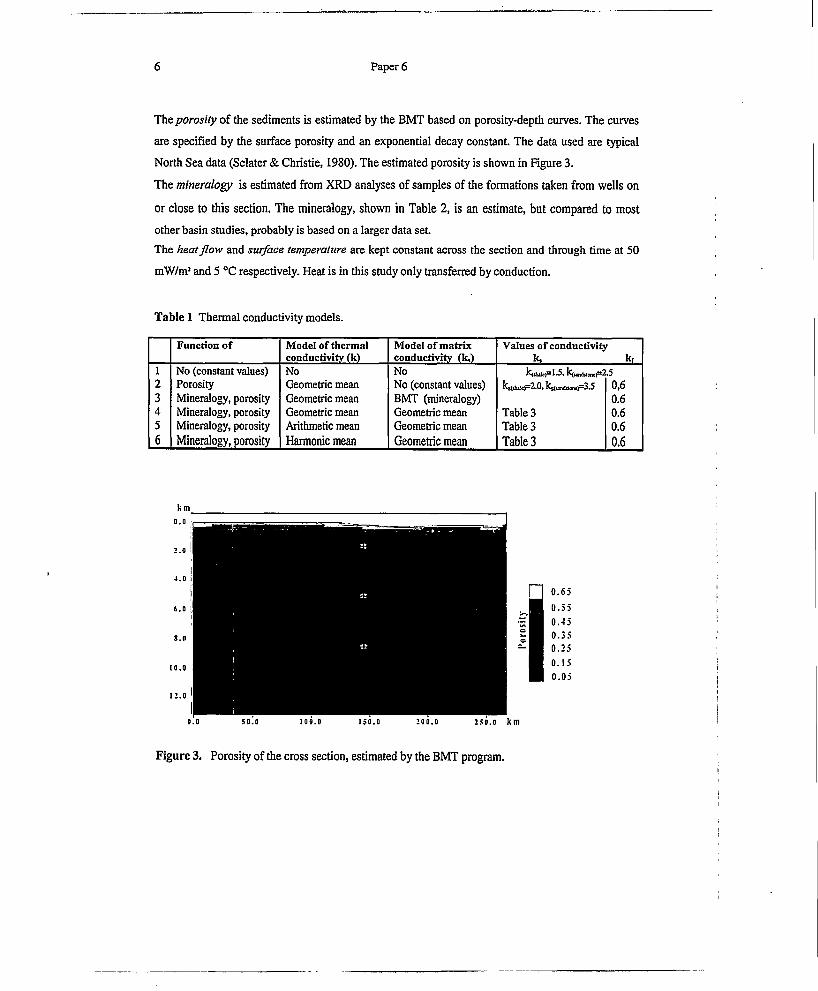
6 Paper 6
The porosity of the sediments is estimated by the BMT based on porosity-depth curves. The curves
are specified by the surface porosity and an exponential decay constant. The data used are typical
North Sea data (Sclater & Christie, 1980). The estimated porosity is shown in Figure 3.
The mineralogy is estimated from XRD analyses of samples of the formations taken from wells on
or close to this section. The mineralogy, shown in Table 2, is an estimate, but compared to most
other basin studies, probably is based on a larger data set.The heat flow and surface temperature are kept constant across the section and through time at 50
mW/m2 and 5 °C respectively. Heat is in this study only transferred by conduction.
Table 1 Thermal conductivity models.
Function of Model of thermal conductivity (k)
Model of matrix conductivity (k,)
Values of conductivityk, kr
1 No (constant values) No No k(ihilc)—1-5. k(undaonefz2.5
2 Porosity Geometric mean No (constant values) k$(ihile)-*2.0, k$(undticnc)r:3.5 0,63 Mineralogy, porosity Geometric mean BMT (mineralogy) 0.64 Mineralogy, porosity Geometric mean Geometric mean Table 3 0.65 Mineralogy, porosity Arithmetic mean Geometric mean Table 3 0.66 Mineralogy, porosity Harmonic mean Geometric mean Table 3 0.6
Figure 3. Porosity of the cross section, estimated by the BMT program.

Table 2 Mineralogy of the formations.
Section Quartz Aik. Fsp. Flag Mica Chlorite I/S Kaolinitc Calcitc Dolom. Sidcrite Pyritc TOC
Quaternary/ Neogene 35 6 5 16 7 7 23 1Paleogene 29 2 6 18 10 9 22 3 1
Carbonaceous Shale 20 2 6 21 8 8 34Upper Jurassic Shale 25 7 7 10 3 10 25 5 1 1 4 2
Brent 31 5 6 8 2 5 27 5 2 3 6
Dunlin Shale 24 5 7 12 3 5 37 1 1 4 1
Statfjord 29 7 16 7 2 2 34 2 1Lunde 30 15 25 2 1 8 14 2 1 1 1
Lomvi 30 15 25 2 1 8 14 2 1
Teist 30 15 25 2 1 8 14 2 1
Permian Sediments 21 21 19 6 5 1 1 1 21 3 1
Sensitivity of therm
al conductivity for temperature history..

8 Paper 6
Table 3. Thermal conductivity of common minerals in sedimentary rocks (Horai, 1971).
MineralThermal
conductivityW/m-K
Quartz 7.8Calcite 3.4Dolomite 5.1Anhydrite 6.4Pyrite 19.2Siderite 3.0K-feldspar 2.3Albite 2.3Mica 2.3Halite 6.5Kaolinite 2.8Elite 1.8Mixed layer I/S 1.9TOC1 0.5
1 Thermal conductivity from BMT database
RESULTS AND DISCUSSION.
Four comparative case studies of temperature histories estimated by six different thermal
conductivity models given in Table 1 are considered.
Case study 1 - The effect of simplified thermal conductivity models.
Temperature histories are modelled from thermal conductivities estimated by Models 1,2 and 3 in
Table 1 are shown in Figure 4. Model 1 is the simplest one. In this model the thermal conductivity
is considered to be constant through the sections. Thermal conductivity is for the shale units set as
1.5 W/m-K and for the sandstone units as 2.5 W/m-K. In Model 2 the matrix conductivity is
considered to be constant through the sections, respectively 2.0 W/m-K for the shale units and 3.5
W/m-K for the sandstone units. Thermal conductivity is estimated by the geometric mean model
based on the estimated porosity data. Thermal conductivity is in Model 3 estimated by the
geometric mean model from the mineralogy and porosity. Matrix conductivity is modelled by
partial least square regression on the basis of a large database (TCD) of measurements on
mineralogy and thermal conductivity. This matrix conductivity estimation is carried out by the
BMT.
For the point representing the Permian a deviation up to 30 K is shown between the simplest model
(Model 1) and the most advanced model (Model 3). The porosity model (Model 2) gives up to 10 K
lower temperature for the Permian than the Model 3. There are only small deviations between

Sensitivity of thermal conductivity for temperature history... 9
240 - Model 1
Temperature History
Model 2(Poroelty model, Penrian) (Poroelty model, Jureesle) (Poroelty model, Tenieiy)
Models(MlnVpor., BMT, Peimlan) (Minypoc, BMT, Juraeile) (MlnVpor, BMT, Teitleiy)
,E 120
-240 -220 -200 -160 -160 -140 -120 -100 -80 -60 -40 -20Age (Ma)
Figure 4. Case study 1. Temperature histories estimated by the two simplest thermal conductivity models (Models 1 & 2) and a model based on thermal conductivity measurements (Model 3).
these two models for the Jurassic and Tertiary points. This comparative case study shows a certain
effect on the temperature history by including the porosity in the thermal conductivity model, while
a further including of the mineralogy in the model gives minor effect on the estimated temperature
history.
Case study 2 - Modelled versus measured thermal conductivities.
Case study 2 shows the temperature histories estimated by Models 3 and 4 (Table 1). Thermal
conductivity are in both models estimated by the geometric mean model from the porosity and mineralogy (Figure 5). The differences lie in the determination of matrix conductivity, k,. Matrix
conductivity in Model 3 is determined from the TCD database of thermal conductivity
measurements and mineralogy, while in Model 4 it is estimated by the geometric mean model from
the mineralogy and the mineral conductivities shown in Table 3.
Using Model 3, the present day temperature profiles for the Permian is estimated about 70 K higher
than that of Model 4. The present day temperature estimated by these two thermal conductivity
models are shown in Figures 6 and 7. The oil window, (ca 100 -140 °C) predicted by Model 3
occurs in the Cretaceous section, while Model 4 predicted this temperature zone lays within the
Jurassic section.
Model 3 is suggested to be more reliable than Model 4 since it depends on measurements of thermal
conductivities. A decrease in the thermal conductivities determined by Model 3 is necessary to get

10 Paper 6
comparable temperature histories by these models. From the assumptions that there is a grain size
effect on the thermal conductivity, and that the mineralogically based geometric mean model (Model
4) estimates too high thermal conductivities for the shale sections, the estimated thermal
conductivities of Model 4 are corrected by a factor of 0.7 for the shale sections (Model 4a) (Figure
8). Usually is the ratio lo,.,Tic, used in basin modelling programs in the range of 0.5 -0.7. A grain
size factor of 0.7 is suggested, since these models is dependent of the mineralogy, and the lower
thermal conductivity of shale sections is assumed to be partly due to a grain size effect and partly
due to a mineralogical effect. The temperature histories estimated by this corrected version of Model
4 (Model 4a) are comparable with those estimated by the model based on measurements (Model 3).
Model 4a gives a slightly higher present day temperature than Model 3 for the Jurassic and Tertiary,
and a lower temperature for the Permian. The highest discrepancy (about 10 K) between these two
models is for the Tertiary.
Including the mineralogical effect of using Model 4 instead of Model 3 in the Case study 1 with the
two simplest models (Models 1 & 2) gives considerably lower temperatures in the sedimentary
section (figure 4). The mineralogy will in this comparison case be an important factor controlling
the temperature history.
Temperature History
Age (Ma)
Models ................. (BMT, Permian). ..
' (BMT, Jurassic)— — — (BMT, Tertiary)
Model4................... (Estimated, Permian)
. (Estimated, Jurassic)— — — (Estimated, Tertiary)
Figure 5. Case study 2. Temperature histories estimated by measured (Model 3) and estimated (Model 4) thermal conductivity models.

Sensitivity of thermal conductivity for temperature history... 11
Figure 6. Present day temperature distribution (°C) of the section estimated by Model 3.
Figure 7. Present day temperature distribution (°C) of the section estimated by Model 4.

12 Paper 6
TemperatureHistory
-240 -220 -200 -180 -160 -140 -120 -100 -80 -60 -40 -20
Age(Ma)
Models • ; .Pehnlan)
(BMT. Jurassic) . 1 —- — — (BMT, Tertiary)
Model* " . >.(Estimated, Pwmian)
"irr’ -.(Estlmeted,Jurassic)■ —- —• (Estimated, Tartiaiy)"..
Model 4a .■ (Estimated,dorr.,Permian)
- (Estimated, corn, Jurassic)
• ~ — - (Estimated, corr-Jeftiary)
Figure 8. Case study 2. Temperature histories estimated by measured (Model 3) and estimated (Model 4) thermal conductivity models and a adjusted version of Model 4, where the shale sections are corrected for the grain size effect of the thermal conductivity (Model 4a).
Case study 3 - Comparison of the three mixing law models.
The consequences of the choice among the three mixing law models (Models 4, 5 & 6) are shown in
Figure 9. The modelled present day temperature conditions within the Permian sediment sequence
varies from 145 °C by using the arithmetic mean model to 230 °C using the harmonic mean model. In
fact the temperature in the Jurassic sediment sequence when modelling with the harmonic mean model
is higher than in the Permian using the arithmetic mean model. Figure 9 shows the importance of
using the correct basic mean model since choosing less fitted model gives a rather biased temperature
history.
In comparison with Model 3 in Case studies 1 and 2 where matrix conductivity is estimated from the
TCD database by the BMT, the harmonic mean model (Model 6) are in best agreement with the
temperature histories estimated by the BMT. Our experience with measuring and modelling thermal
conductivities is that the arrangement of the fluid and matrix component due to the direction of heat
flow has minor effect on the thermal conductivity (Midtt0mme & Roaldset, 1997a). From this reason
we prefer the geometric mean model instead of the harmonic mean model.

Sensitivity of thermal conductivity for temperature history... 13
Temperature History
-240 -220 -200 -180 -160 -140 -120 -100 -60 -60 -40 -20Age(Ma)
Model 4.............. (Geometric mean, Petmtan)
(Geometric mean, Jurassic)
— — — (Geometric mean, Tertiary)
Models.. (Arithmetic mean, Permian)--------- - (Arithmetic mean, Jurassic)
-- (Arithmeticmean, Tertiary)
Model B.. (Hanrontemean, Patmten)
1 ■ (Harmonic mean, Jurassic)
—• — — (Harmonic mean, Tertiary)
Figure 9. Case study 3. Temperature histories estimated by the three mixing law models; geometric (Model 4); arithmetic (Model 5) and harmonic (Model 6) mean models.
Case study 4 - The effect of varying the thermal conductivity of the Brent Group.Thermal conductivity is in Figure 10 estimated by Model 3, the geometric mean model based on
BMT database of thermal conductivity measurements and mineralogy. The differences in these three
scenarios are in the thermal conductivity of Brent Group which is set as a constant: a) 2.25
W/m-K, which is approximately the mean thermal conductivity of this section estimated by Model 3;
b) k,^r= 1.5 W/m-K, and c) &,**= 3.0 W/m-K respectively. Because of a the many coal beds in the
Brent Group, this thermal conductivity is associated with more uncertainty than those of the other
formations (Midtt0mme et al., 1996). The Brent Group along this cross-section is thinner than many
of the other formations, and will certainly have less effect on the temperature history than the thicker
formations.
The variation of thermal conductivity of the Brent Group has a small effect on the temperature
history (Figure 10). Only for the Permian sediments is any discrepancy in the three temperature
histories indicated. The largest discrepancy is 8 K between the scenario with highest and lowest
thermal conductivity in the time period 100 -160 Ma.

14 Paper 6
Temperature History
■240 -220 -200 -180 -160 -140 -120 -100 -80 -60 -40 -20
Age(Ma)
2 (Brent k»2.25t Permian)
:p-*rri (Br^M^ Jumsslc) ..-r—• s (Brent k*<2£5, Tertteiy)
• Mode! 3b , I.(Brent k=1^5j Permian)
(Brent MiS, Jurassic)
. T ' (Brent k=1.5,Tertiaiy)f'
./Model 3c \ - . ' //;. 7' (Brent k=3.0,. Permian)
-1' ■ „; (Brent k=3.0, Jurassic)*— — .(Brent k=3.0, Tertiary)
Figure 10. Case study 4. Temperature histories estimated with different thermal conductivities of the Brent Group.
CONCLUSION.
Considerable deviation in the estimated temperature histories is demonstrated by using different
thermal conductivity models. Simplified models, which only take account of either the lithology
(Model 1) or the lithology and porosity (Model 2), give a good estimate of the temperature history
compared to more advanced models. The largest discrepancy in temperature histories appears in the
mutual comparison between more advanced thermal conductivity models, which are based on
mineralogy and porosity. Model 3 is suggested to be the most reliable model. In this model matrix
conductivity, k,. is based on a database of measured thermal conductivities (TCD)by the BMT
programme. Model 3 gives considerably higher temperatures than Model 4 where matrix conductivity
is estimated by the geometric mean model based on the mineralogy. A grain size correction of the
geometric mean model (Model 4) of the shale units gives comparable thermal histories with the BMT
model (Model 3). Using the three statistical mean models, respectively arithmetic mean, geometric
mean and harmonic mean as basic model for estimating the thermal conductivity give very different
temperature histories. Varying the thermal conductivity for the Brent Group has little effect on the
modelled temperature histories.
Sensitivity of thermal conductivity for temperature history... 15
REFERENCES.
Bergsager, E., 1986 Character of the North Sea. In: A. Bang-Andersen et al. (eds.) The North Sea. A Highwayof Economic and Cultural Exchange. Character-History. Nor. Univ. Press.
Blackwell, D. D. & Steele, J. L. 1989. Thermal conductivity of sedimentary rocks: measurements and significance. In: Naeser, N. D. & McCulloh, T. H. (eds) Thermal History of Sedimentary Basins, Methods and Case Histories. Springer Verlag, New York, 13-36.
Demongodin, L., Pinoteau, B., Vasseur, G. & Gable, R. 1991. Thermal conductivity and well logs: a case study in the Paris Basin. Geophysical Journal International, 105, 675-691.
Fjeldskaar, W., Prestholm, E., Guargena, G. & Gravdal, N. 1993. Isostatic and tectonic subsidence of the Egersund Basin. In Dor6 A.G. et al (eds.) Basin Modelling: Advances and Applications, Norwegian Petroleum Society Special Publication No. 3. Elsevier, Amsterdam, 549-562
Gallagher, K., Ramsdale, M., Lonergan, L. & Morrow, D. 1997. The role of thermal conductivity measurements in modelling thermal histories in sedimentary basins. Marine and Petroleum Geology, 14, 201-214.
Horai, K.I. 1971, Thermal conductivity of rock-forming minerals. Journal of Geophysical Research. 76, 1278-1308.
Johansen, H., Fjeldskaar, W. & Mykkeltveit, J. 1995. The influence of glaciation on the basin temperature regime. Global and Planetary Change, 12,437-448.
Lander, R. H., Fjeldskaar, W. & Johansen, H. 1994. Sensitivity of modelled temperature and hydrocarbon maturation to structural restoration in growth faulted settings. The Geological Society Petroleum Group Conference on Basin Modelling.
McCulloh, T.H. & Naeser, N.D. 1989. Thermal History of Sedimentary Basins: Introduction and Overview. In: Naeser, N. D. & McCulloh, T. H. (eds) Thermal History of Sedimentary Basins, Methods and Case Histories. Springer Verlag, New York, 1-11.
McKenna, T. E., Sharp, J. M. Jr., & Lynch, F.L. 1996. Thermal conductivity of Wilcox and Frio sandstones in south Texas (Gulf of Mexico Basin). AAPG Bulletin, 80,1203-1215.
Midttemme, K., Roaldset, E. and Brant}es, J.G. 1996. Thermal conductivity of alluvial sediments from the Ness Formation, Oseberg Area, North Sea. EAEG 58th Conference, Extended Abstracts Volume 2, P552, Amsterdam.
Midttemme, K., Roaldset, E. & Aagaard, P. 1997a. Thermal conductivity of selected clay- and mudstones from England, Clay Minerals, 33, 131-145.
Midttemme, K., Ssttem, J. & Roaldset, E. 1997b. Thermal conductivity of unconsolidated marine sediments from Vering Basin, Norwegian Sea. In: Middleton M.F. (ed.) Nordic Petroleum Technology Series: Two, Nordisk energiforskningssamarbejde. in press.
Midttemme, K. & Roaldset, E. 1997a. Thermal conductivity of sedimentary rocks - uncertainties in measuring and modelling. Submitted to Mudrocks at Basin Scale. Properties, Controls and Behaviour, Geological Society Special Publication.
Midttemme, K. & Roaldset, E. 1997b. The effect of grain size on thermal conductivity of quartz sands and silts. Petroleum Geoscience, in press.
Rzhevsky, V. & Novik, G. 1971. The Physics of Rocks. Mir Publishers, Moscow, (translated from the Russian by Chatteijee, A. K).

16 Paper 6
Rundberg, Y., 1991. Tertiary sedimentary history and basin evolution of the Norwegian North Sea between 60 - 62° N an integrated approach. Dr. ing thesis, Department of Geology and Mineral Resources Engineering, Norwegian Institute of Technology, rep.25, Trondheim.
Sciater, J.G. & Christie, P.A.F. 1980, Continental stretching: an explanation of the post-mid-cretaceous subsidence of the central north sea basin. Journal of Geophysical Research, 85, B7,3711-3739.
Somerton, W.H. 1992. Thermal properties and temperature related behavior of rock/fluid systems. Developements in Petroleum Sciences, 37, Elsevier, Amsterdam.