Embed Size (px)
Citation preview
THERMAL ANALYSIS OF A POPPET
VALVE GASOLINE ENGINE FOR
TWO- AND FOUR-STROKE
OPERATION
ALEXIS G. DEL RIO GONZALEZ
Master of Philosophy
June 2010

Acknowledgements
I would like to thank all those people who contributed to my work in order of importance,
while I apologise if I did not mentioned you.
First I would like to thank to my supervisors, Dr. Steven Begg, positive feedback without
him this would have been literally impossible. Dr. David Mason, for his time and
patience with my spread sheet calculations and advice during all this time. Also I want to
thank those supervisors that came and went Prof. Tim Cowell, for keeping me focused
and making me to work to the maximum. Dr. Walid Abdelghaffar, for his help and
support with the software and natural interest in my work.
Second I would like to thank those within the university Mr. Bill Whitney, Mr. Ken
Maris and Mr. Brian Maggs for creating such a great test cell engine. Dr. Nicolas Miche,
for his interest in the subject and support on getting the engine required information. Mr.
Dave Stansbury, for his computer expertise. Mr. Aidan Delaney, for his out of work help
with the cluster. Prof. Alison. M. Bruce for her kindness with University matters.
Third from outside university I would like to thank Mr. Neil Brown, for his support
during the part time studies. Mr. Richard Penning, from the Ricardo helpdesk for his
support with the fluid dynamics software.
Finally and most important of all:
Este trabajo esta dedicado a mi convaleciente padre; Armando del Rio Llabona también
a mi madre; Ana Maria Gonzalez y en especial a mi hermano; Ciro del Rio y mi
cuñada; Gemma Zurita por su siempre incondicional apoyo.
This work is dedicated to my father Armando del Rio Llabona who is convalescent, also
to my mother Ana Maria Gonzalez while special thanks are for my brother Ciro del Rio
and my sister-in-law Gemma Zurita because of their backing.
Thank you all
Declaration
I declare that the research contained in this thesis, unless otherwise formally indicated
within the text, is the original work of the author. The thesis has not been previously
submitted to this or any other university for a degree, and does not incorporate any
material already submitted for a degree.
Signed
Dated
1
Abstract
The modern four-stroke, poppet valve, direct injection, gasoline engine has improved
combustion efficiency, reduced emissions and greater engine performance when
compared to the port-fuel injected engine. In parallel, two-stroke, piston-ported
engine designs have also evolved. However, their greater pollution levels have limited
their potential in the market. Two-stroke operation offers higher specific power output
than four-stroke, while at part load, four-stroke operation offers better fuel
consumption. Therefore, a combination of the two operating systems, in a poppet
valve engine design, presents a potential solution to these problems. On the other
hand, two-stroke engine operation generates more power and torque and the
corresponding heat transfer is higher. For four-stroke engines, thermal studies have
historically been carried out on many different types of engines. In contrast, two-
stroke, poppet valve engine thermal studies are very limited. However, recently, the
DTI funded 2/4 SIGHT engine programme has resulted in the construction of a
poppet valve experimental research engine, which can switch between two- and four-
stroke operation depending on the throttle and engine load demands. This represents a
novel situation as the same engine configuration is used for both firing operations. In
this study, the heat transfer was considered for engine operation at four- and two-
stroke peak torque conditions, where the maximum in-cylinder heat flux occurs at
peak combustion temperatures. The engine was operated under steady-state conditions
where thermal equilibrium was achieved at each engine speed and load. A quasi-
steady, average heat flux approximation was considered over the combustion chamber
surfaces. Experimental data were collected for both steady-state (averaged over
consecutive engine cycles) and at instantaneous crank angles. The steady-state
temperature difference between the coolant at the engine inlet and outlet was used to
calculate a difference term between the ideal combustion chamber energy balance and
the calculated heat flux results. The results were compared with correlations identified
in the literature; in particular, for heat flux (Annand and Ma, (1972)) and heat transfer
coefficient (Woschni, (1967)). In addition, the Ricardo empirical heat flux expression
for four-stroke operation was also considered for four-stroke and then compared to
two-stroke operation. Finally, a two-stroke correction factor was proposed that took
into account the engine torque, air to fuel ratio and mean piston speed terms.
2
List of contents
Abstract..................................................................................................................... 1
List of contents.......................................................................................................... 2
List of Figures ........................................................................................................... 5
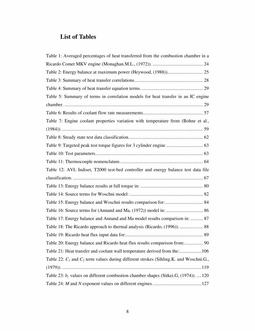
List of Tables ............................................................................................................ 8
Nomenclature/Abbreviations ..................................................................................... 9
1 Introduction ..................................................................................................... 13
2 Literature review ............................................................................................. 14
2.1 Introduction ............................................................................................. 14
2.2 Description of the research problem;........................................................ 25
2.3 Dimensional analysis and empirical correlation........................................ 28
2.4 Empirical heat transfer coefficient correlations......................................... 30
2.4.1 Radiation.......................................................................................... 30
2.4.2 Forced convection ............................................................................ 30
2.4.3 Characteristic dimensions................................................................. 30
2.4.4 Gas properties & motored operation ................................................. 33
2.4.5 Instantaneous temperature measured values...................................... 34
2.5 Empirical heat flux correlations ............................................................... 34
2.5.1 Radiation term.................................................................................. 34
2.5.2 Forced convection ............................................................................ 36
2.5.3 Characteristic dimensions................................................................. 36
2.5.4 Gas properties & motored operation ................................................. 36
2.5.5 Instantaneous temperature measured values...................................... 37
2.6 Conclusions of literature review............................................................... 38
2.6.1 Summary of models ......................................................................... 40
2.7 Description of thesis ................................................................................ 42
3 Experimental studies........................................................................................ 44
3.1 Introduction ............................................................................................. 44
3.2 Experimental research engine facility....................................................... 44
3.3 Data logging (high-speed / low-speed). .................................................... 46
3.3.1 Research engine and instrumentation................................................ 46
3.4 Thermal Survey ....................................................................................... 53
3
3.4.1 Cooling Strategy .............................................................................. 53
3.4.2 Coolant Fluid Properties................................................................... 57
3.4.3 Thermal instrumentation .................................................................. 59
3.5 Experimental method ............................................................................... 61
3.5.1 Operating conditions ........................................................................ 61
3.5.2 Data Logging ................................................................................... 62
4 Experimental results ........................................................................................ 66
4.1 Summary of engine performance.............................................................. 66
4.2 Data analysis............................................................................................ 73
4.2.1 Working assumptions....................................................................... 74
4.2.2 Calculation procedure....................................................................... 78
4.2.3 Heat Transfer Coefficient correlations .............................................. 78
4.2.4 Heat Flux correlations ...................................................................... 85
4.2.5 The Ricardo Empirical Heat Flux Factor (Q/F)................................. 88
4.2.6 Conclusions of the research methods ................................................ 96
4.2.7 Four-Stroke Operation...................................................................... 98
4.2.8 Two-stroke Operation......................................................................101
4.3 Comparison with available data ..............................................................105
5 Conclusions....................................................................................................110
6 Recommendations for further work.................................................................112
7 References......................................................................................................113
8 Appendices.....................................................................................................115
8.1 Appendix A ............................................................................................115
Heat transfer correlations........................................................................................115
8.1.1 Nusselt’s Correlation 1923 ..............................................................115
8.1.2 Eichelberg’s Correlation 1939 .........................................................115
8.1.3 Oguri’s Correlation 1960.................................................................116
8.1.4 Pflaum’s Correlation 1963...............................................................117
8.1.5 Annand’s Correlation 1962, 1971....................................................118
8.1.6 Woschni’s Correlation 1967, 1979 ..................................................118
8.1.7 Sitkei’s Correlation 1974.................................................................120
8.1.8 Dent’s Correlation 1977 ..................................................................121
8.1.9 Hohemberg’s Correlation 1980........................................................122
8.1.10 Lawton’s Correlation 1987..............................................................123
4
8.1.11 Kouremenos’s Correlation 1988 ......................................................124
8.1.12 Imabeppu’s Correlation 1993 ..........................................................125
8.1.13 The Ricardo Empirical Heat Flux Correlation 1996 .........................125
8.1.14 Han’s Correlation 1997 ...................................................................127
8.2 Appendix B.............................................................................................129
Heat Flux Calculation.............................................................................................129

5
List of Figures
Figure 1: Schematic of the four-stroke cycle (Ricardo, (2008)). ............................... 15
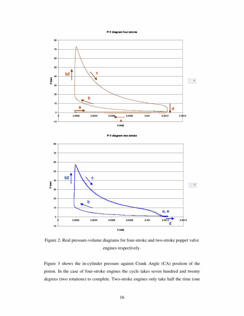
Figure 2: Real pressure-volume diagrams for four-stroke and two-stroke poppet valve
engines respectively. ............................................................................................... 16
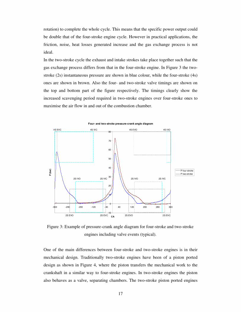
Figure 3: Example of pressure-crank angle diagram for four-stroke and two-stroke
engines including valve events (typical). ................................................................. 17
Figure 4: Example of schematic of physical two-stroke piston ported engine design
(Heywood, (1988)). ................................................................................................. 18
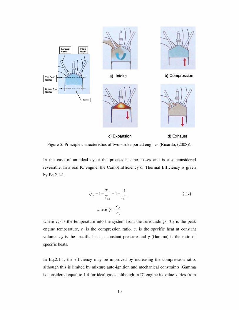
Figure 5: Principle characteristics of two-stroke ported engines (Ricardo, (2008)). .. 19
Figure 6: Energy balance system. ............................................................................ 21
Figure 7: Schematic of heat transfer through the cylinder head in a poppet valve IC
engine (Bywater and Timmins, (1980)). .................................................................. 24
Figure 8: Temperature distribution diagram............................................................. 26
Figure 9: Test cell and control room overall view. ................................................... 45
Figure 10: Overview of instrumentation set-up. ....................................................... 46
Figure 11: Engine test bed 2/4SIGHT, 3-cylinder, direct injection, gasoline engine. 47
Figure 12: Valve control unit & pressure pump. ...................................................... 47
Figure 13: Monitoring PC........................................................................................ 48
Figure 14: AVL Indiset front and rear view. ............................................................ 49
Figure 15: Ricardo Test Automation T2000 test-bed controller................................ 50
Figure 16: Piezoelectric pressure transducer. ........................................................... 51
Figure 17: Charge amplifier..................................................................................... 52
Figure 18: Microstrain interface. ............................................................................. 52
Figure 19: Max flow meter (courtesy of Maxmachinery) ......................................... 53
Figure 20: Engine coolant core view from piston top, inlet port and exhaust port..... 54
Figure 21: Cylinder head thermocouple positions and coolant flow direction........... 55
Figure 22: Cylinder block thermocouple positions and coolant flow direction. ........ 55
Figure 23: Section A-A through coolant transfer passage of exhaust valve bridge.... 56
Figure 24: Type K thermocouple. ............................................................................ 60
Figure 25: Low speed data logger. ........................................................................... 61
Figure 26: Predicted V6 full load performance target for two and four-stroke
operation (from 2/4SIGHT, 2008). .......................................................................... 62
6
Figure 27: Example of One Dimensional Correlation Spread Sheet, based upon the
Ricardo Heat Flux Formula. .................................................................................... 65
Figure 28: Engine overall operating strategy from (Ricardo, (2008)). ...................... 66
Figure 29: Engine topology (Ricardo, (2008)). ........................................................ 67
Figure 30: Typical example of four-stroke engine performance: AVL Indiset data at
1000rpm, 1500 and 2000rpm at peak torque. ........................................................... 68
Figure 31: Typical example of two-stroke engine performance: AVL Indiset data at
1000-1500-2000-2500rpm at peak torque. ............................................................... 69
Figure 32: Two- and four-stroke fuel injection comparison over 720 degCA between
1000-2000 rpm tests, with constant fuel injection pressure and lambda.................... 70
Figure 33: Mean gas pressure, pi and estimated temperature, Ti simulated using
WAVE, for a 0.3 litre single cylinder, two-stroke, poppet valve, spark ignition engine,
with a 11:1 compression ratio at 2500 rpm. ............................................................. 73
Figure 34: Overview of thermal studies. .................................................................. 74
Figure 35: The Ricardo top entry poppet valve reverse tumble gas motion............... 75
Figure 36: A section through the exhaust-exhaust valve bridge showing the steady-
state coolant flow velocity profiles. The simulation was performed using the Ricardo
Vectis CFD software (courtesy of Ricardo). ............................................................ 76
Figure 37: Four-stroke partially throttled motored pressure data; from the T2000
24CAR-022 and Indiset test 24CAR-1022 at 2500rpm. ........................................... 82
Figure 38: Two-stroke partially throttled motored pressure data: from Indiset test
TFS027-005 at 2500rpm.......................................................................................... 83
Figure 39: Ricardo heat flux combustion chamber variation from bore center for: ... 91
Figure 40: Effect of AFR on the heat flux “F Factor” for gasoline engines (Ricardo,
(1996)). ................................................................................................................... 92
Figure 41: Full torque thermocouple temperature for:.............................................. 94
Figure 42: “F Factor” variation with heat flux in:................................................... 96
Figure 43: Comparison of four-stroke net heat flux results at peak torque of: 1000rpm,
80Nm; 1500 rpm, 126Nm; and 2000rpm, 167Nm.................................................... 99
Figure 44: Variation in exhaust manifold temperature across cylinders for: ............100
Figure 45: Variation in two-stroke net heat flux results at peak torque for: 1000 to
2500rpm.................................................................................................................102
7
Figure 46: Two-stroke Torque and apparent Lambda_ECM (λECM) results for:
1000rpm and 136Nm of torque; 1500rpm and 192Nm; 2000rpm and 231Nm; and
2500rpm and 252Nm..............................................................................................103
Figure 47: Variation in the correction factor for Ricardo geometrical heat flux results
in two-stroke operation for: 1000rpm, 136Nm; 1500rpm, 192Nm; 2000rpm, 231Nm;
and 2500rpm, 252Nm.............................................................................................104
Figure 48: Corrected Ricardo two-stroke results compared to the energy balance for:
1000rpm, 136Nm; 1500rpm, 192Nm; 2000rpm, 231Nm; and 2500rpm, 252Nm.....105
Figure 49: Two- and four-stroke operation coolant wall temperature (Tw,c) results
from: energy balance (theoretical balance) and coolant flow calculation (based on
experiment). ...........................................................................................................108
Figure 50: Temperature variation in the surface of the cylinder head coolant jacket,
for a Ford Valencia 1.1 gasoline engine, from 10 to 62Nm and 1500 to 3500rpm
(Stone, (1999)), compared to coolant flow calculation (Xa) and energy balance results
(Xb). ......................................................................................................................109
Figure 51: Variation of F Factor depending on location (Ricardo, (1996)). .............126
Figure 52: Heat Flux Calculation Spread Sheet.......................................................129
8
List of Tables
Table 1: Averaged percentages of heat transferred from the combustion chamber in a
Ricardo Comet MKV engine (Monaghan.M.L., (1972)). ......................................... 24
Table 2: Energy balance at maximum power (Heywood, (1988))............................. 25
Table 3: Summary of heat transfer correlations........................................................ 28
Table 4: Summary of heat transfer equation terms. .................................................. 29
Table 5: Summary of terms in correlation models for heat transfer in an IC engine
chamber. ................................................................................................................. 29
Table 6: Results of coolant flow rate measurements................................................. 57
Table 7: Engine coolant properties variation with temperature from (Bohne et al.,
(1984)). ................................................................................................................... 59
Table 8: Steady state test data classification............................................................. 62
Table 9: Targeted peak test torque figures for 3 cylinder engine .............................. 63
Table 10: Test parameters........................................................................................ 63
Table 11: Thermocouple nomenclature.................................................................... 64
Table 12: AVL Indiset, T2000 test-bed controller and energy balance test data file
classification. .......................................................................................................... 67
Table 13: Energy balance results at full torque in: ................................................... 80
Table 14: Source terms for Woschni model: ............................................................ 82
Table 15: Energy balance and Woschni results comparison for:............................... 84
Table 16: Source terms for (Annand and Ma, (1972)) model in: .............................. 86
Table 17: Energy balance and Annand and Ma model results comparison in: .......... 87
Table 18: The Ricardo approach to thermal analysis (Ricardo, (1996)). ................... 88
Table 19: Ricardo heat flux input data for:............................................................... 89
Table 20: Energy balance and Ricardo heat flux results comparison from:............... 90
Table 21: Heat transfer and coolant wall temperature derived from the:..................106
Table 22: C1 and C2 term values during different strokes (Sihling.K. and Woschni.G.,
(1979)). ..................................................................................................................119
Table 23: bc values on different combustion chamber shapes (Sitkei.G, (1974)). ....120
Table 24: M and N exponent values on different engines. .......................................127
9
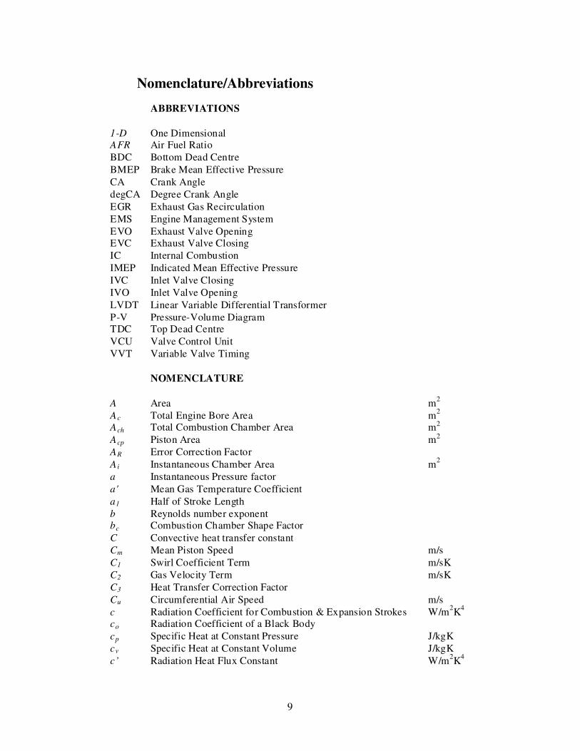
Nomenclature/Abbreviations
ABBREVIATIONS
1-D One Dimensional
AFR Air Fuel Ratio
BDC Bottom Dead Centre
BMEP Brake Mean Effective Pressure
CA Crank Angle
degCA Degree Crank Angle
EGR Exhaust Gas Recirculation
EMS Engine Management System
EVO Exhaust Valve Opening
EVC Exhaust Valve Closing
IC Internal Combustion
IMEP Indicated Mean Effective Pressure
IVC Inlet Valve Closing
IVO Inlet Valve Opening
LVDT Linear Variable Differential Transformer
P-V Pressure-Volume Diagram
TDC Top Dead Centre
VCU Valve Control Unit
VVT Variable Valve Timing
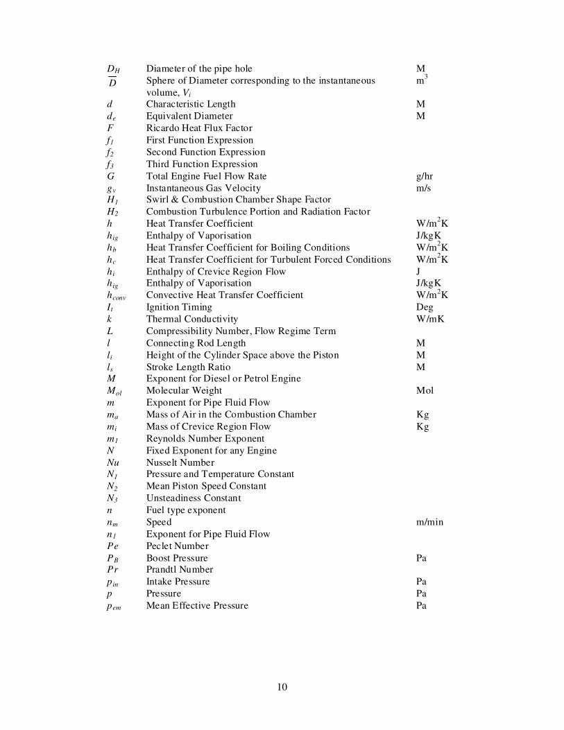
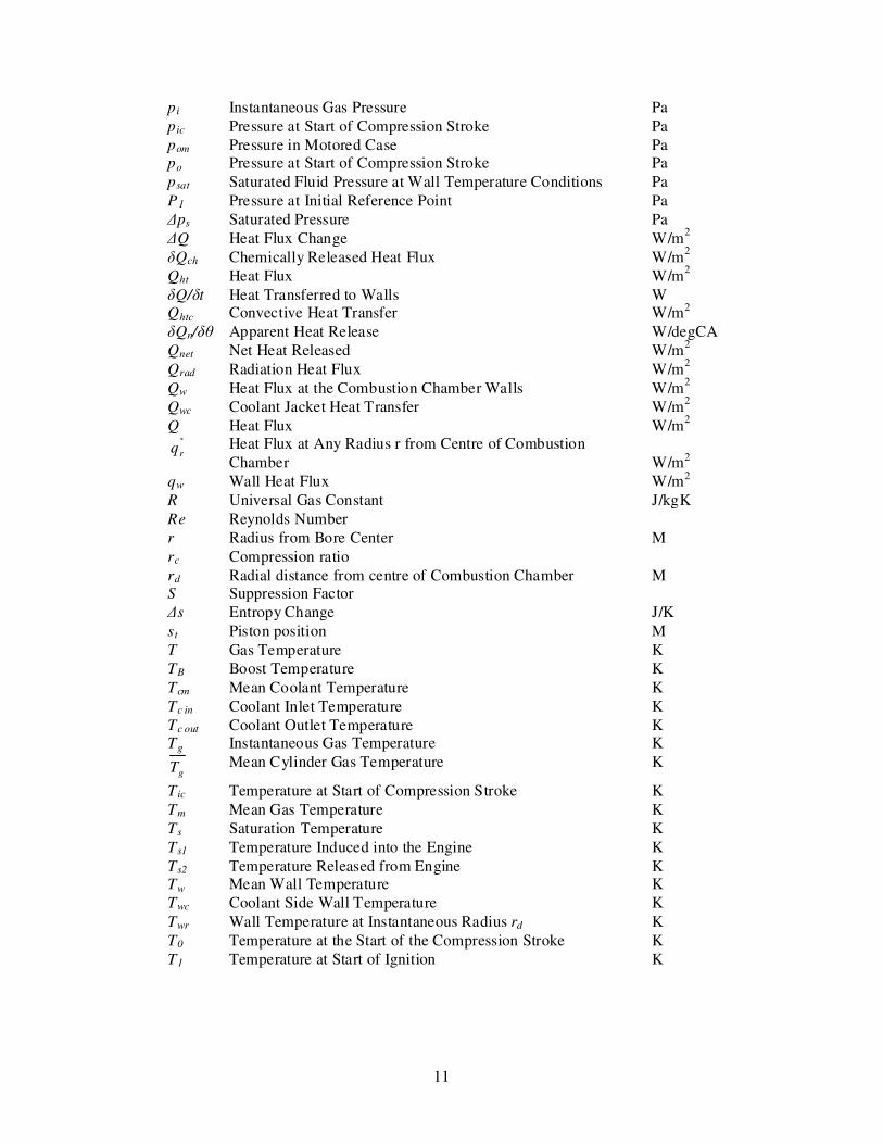
NOMENCLATURE
A Area m2
Ac Total Engine Bore Area m2
Ach Total Combustion Chamber Area m2
Acp Piston Area m2
AR Error Correction Factor
A i Instantaneous Chamber Area m2
a Instantaneous Pressure factor
a' Mean Gas Temperature Coefficient
a1 Half of Stroke Length
b Reynolds number exponent
bc Combustion Chamber Shape Factor
C Convective heat transfer constant
Cm Mean Piston Speed m/s
C1 Swirl Coefficient Term m/sK
C2 Gas Velocity Term m/sK
C3 Heat Transfer Correction Factor
Cu Circumferential Air Speed m/s
c Radiation Coefficient for Combustion & Expansion Strokes W/m2K
4
co Radiation Coefficient of a Black Body
cp Specific Heat at Constant Pressure J/kgK
cv Specific Heat at Constant Volume J/kgK
c’ Radiation Heat Flux Constant W/m2K
4
10
DH Diameter of the pipe hole M
D Sphere of Diameter corresponding to the instantaneous
volume, Vi
m3
d Characteristic Length M
de Equivalent Diameter M
F Ricardo Heat Flux Factor
f1 First Function Expression
f2 Second Function Expression
f3 Third Function Expression
G Total Engine Fuel Flow Rate g/hr
gv Instantaneous Gas Velocity m/s H1 Swirl & Combustion Chamber Shape Factor
H2 Combustion Turbulence Portion and Radiation Factor
h Heat Transfer Coefficient W/m2K
h ig Enthalpy of Vaporisation J/kgK
hb Heat Transfer Coefficient for Boiling Conditions W/m2K
hc Heat Transfer Coefficient for Turbulent Forced Conditions W/m2K
h i Enthalpy of Crevice Region Flow J h ig Enthalpy of Vaporisation J/kgK
hconv Convective Heat Transfer Coefficient W/m2K
It Ignition Timing Deg
k Thermal Conductivity W/mK
L Compressibility Number, Flow Regime Term
l Connecting Rod Length M
li Height of the Cylinder Space above the Piston M
ls Stroke Length Ratio M M Exponent for Diesel or Petrol Engine
Mol Molecular Weight Mol
m Exponent for Pipe Fluid Flow
ma Mass of Air in the Combustion Chamber Kg
mi Mass of Crevice Region Flow Kg
m1 Reynolds Number Exponent
N Fixed Exponent for any Engine
Nu Nusselt Number N1 Pressure and Temperature Constant
N2 Mean Piston Speed Constant
N3 Unsteadiness Constant
n Fuel type exponent
nm Speed m/min
n1 Exponent for Pipe Fluid Flow
Pe Peclet Number
PB Boost Pressure Pa Pr Prandtl Number
p in Intake Pressure Pa
p Pressure Pa
pem Mean Effective Pressure Pa
11
p i Instantaneous Gas Pressure Pa
p ic Pressure at Start of Compression Stroke Pa
pom Pressure in Motored Case Pa po Pressure at Start of Compression Stroke Pa
psat Saturated Fluid Pressure at Wall Temperature Conditions Pa
P1 Pressure at Initial Reference Point Pa
∆ps Saturated Pressure Pa
∆Q Heat Flux Change W/m2
δQch Chemically Released Heat Flux W/m2
Qht Heat Flux W/m2
δQ/δt Heat Transferred to Walls W Qhtc Convective Heat Transfer W/m2
δQn/δθ Apparent Heat Release W/degCA
Qnet Net Heat Released W/m2
Qrad Radiation Heat Flux W/m2
Qw Heat Flux at the Combustion Chamber Walls W/m2
Qwc Coolant Jacket Heat Transfer W/m2
Q Heat Flux W/m2
''
rq Heat Flux at Any Radius r from Centre of Combustion
Chamber W/m2
qw Wall Heat Flux W/m2
R Universal Gas Constant J/kgK
Re Reynolds Number
r Radius from Bore Center M
rc Compression ratio
rd Radial distance from centre of Combustion Chamber M S Suppression Factor
∆s Entropy Change J/K
st Piston position M
T Gas Temperature K
TB Boost Temperature K
Tcm Mean Coolant Temperature K
Tc in Coolant Inlet Temperature K
Tc out Coolant Outlet Temperature K Tg Instantaneous Gas Temperature K
gT Mean Cylinder Gas Temperature K
T ic Temperature at Start of Compression Stroke K
Tm Mean Gas Temperature K
Ts Saturation Temperature K
Ts1 Temperature Induced into the Engine K
Ts2 Temperature Released from Engine K Tw Mean Wall Temperature K
Twc Coolant Side Wall Temperature K
Twr Wall Temperature at Instantaneous Radius rd K
T0 Temperature at the Start of the Compression Stroke K
T1 Temperature at Start of Ignition K
12
T2 Temperature at Final Reference Point K
t Time S
t0 Piston Speed m/s dUc Internal Energy Change J
Ud Mean Flow Velocity m/s
u Characteristic Velocity
u' Turbulent Viscosity in Pre-chamber m/s
V Volume Chamber m3
VH Swept Volume m3
V i Instantaneous Cylinder Volume m3
V1 Cylinder Volume at Start of Ignition m3
v Characteristic Velocity m/s
v& Volumetric Flow Rate m3/s
δW Brake Engine Work J
w In Cylinder Mean Gas Velocity affecting Heat Transfer
GREEK LETTERS
α Thermal Diffusivity W/mK
β Emissivity Correction Factor
2COε Emissivity of Carbon Dioxide
OH2ε Emissivity of Water
εg Gas Emissivity
εo Emissivity Coefficient
εr Non-steady to Quasi-steady Heat Flux Error
γ Ratio of Specific Heats
η Polytropic Process Constant
η th Carnott (Thermal) Efficiency
λ Lambda λECM Lambda Corrected Signal
µ Dynamic Fluid Viscosity Pa .s
θ Crank Angle Deg
θr Rotational Engine Speed Rpm
ρ Gas Density kg/m3
Aρ Atmospheric Air Density kg/m
3
Iρ Inlet Air Density kg/m3
σ Stefan-Boltzmann Constant W/m2K4
σ t Surface Tension N/m
υ Kinematic Viscosity kg/ms
ω Air Swirl Motion rad/s
ωf Crankshaft Angular Frequency s-1
ωs Tangential Gas Velocity m/s
13
1 Introduction
Two- and four-stroke engines have different capabilities that may be desirable to
combine. For a same engine volume, four-stroke generate a better part load
consumption while two-stroke engines gives higher specific power and torque output.
For this to happen in four-stroke operation, the engine volume needs to be at least
double of that of the two-stroke mode. This requires higher fuel consumption, bigger
and heavier parts that may not be economically produced. For a similar engine
displacement although two-stroke operation consumes more fuel than the four-stroke
option, this is effectively lower than increasing the engine displacement. On the
negative side, two-stroke piston ported engines produce higher levels of pollutants
than the four-stroke ones, which is obtained at the expense of having more engine
components. A possibility of overcoming their problems is to run a poppet valve
spark ignition internal combustion engine configuration. In this case the main problem
is the camshaft timing operation and configuration to allow for the increase/decrease
of the camshaft speed when varying between the firing operations. This is obtained by
running an electro-hydraulic valve actuation system, where the firing operations are
selected in terms of the load and the throttle requirements.
Since the cycle frequency and the fuel consumption made the thermal requirements of
the two cycles different, this engine became an ideal tool for an in depth thermal
analysis. This analysis comprehended the maximum torque requirements for both
firing operations at 1000, 1500 and 2000rpm in four-stroke operation, while it also
included a case in 2500rpm for two-stroke operation. The energy balance calculation
was determined for each operation and then compared to those heat fluxes from
Annand and Ma, (1972), Woschni, ((1967) and Ricardo (1996) calculations. This
analysis allowed finding what requirements the Ricardo heat flux model needed to
accurately quantify the two-stroke operation. These results were then corrected
through a comparison of; the energy balance temperature results at the coolant wall,
together with the energy released into the coolant from the test cell results. These
results allowed obtaining an error percentage that was implemented in the Ricardo
two-stroke operation model correction obtaining similar results to those in the energy
balance.
14
2 Literature review
2.1 Introduction
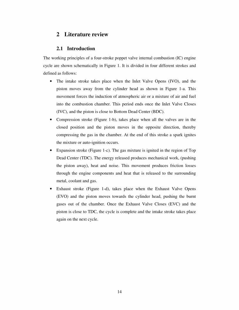
The working principles of a four-stroke poppet valve internal combustion (IC) engine
cycle are shown schematically in Figure 1. It is divided in four different strokes and
defined as follows:
• The intake stroke takes place when the Inlet Valve Opens (IVO), and the
piston moves away from the cylinder head as shown in Figure 1-a. This
movement forces the induction of atmospheric air or a mixture of air and fuel
into the combustion chamber. This period ends once the Inlet Valve Closes
(IVC), and the piston is close to Bottom Dead Center (BDC).
• Compression stroke (Figure 1-b), takes place when all the valves are in the
closed position and the piston moves in the opposite direction, thereby
compressing the gas in the chamber. At the end of this stroke a spark ignites
the mixture or auto-ignition occurs.
• Expansion stroke (Figure 1-c). The gas mixture is ignited in the region of Top
Dead Center (TDC). The energy released produces mechanical work, (pushing
the piston away), heat and noise. This movement produces friction losses
through the engine components and heat that is released to the surrounding
metal, coolant and gas.
• Exhaust stroke (Figure 1-d), takes place when the Exhaust Valve Opens
(EVO) and the piston moves towards the cylinder head, pushing the burnt
gases out of the chamber. Once the Exhaust Valve Closes (EVC) and the
piston is close to TDC, the cycle is complete and the intake stroke takes place
again on the next cycle.
15
Figure 1: Schematic of the four-stroke cycle (Ricardo, (2008)).
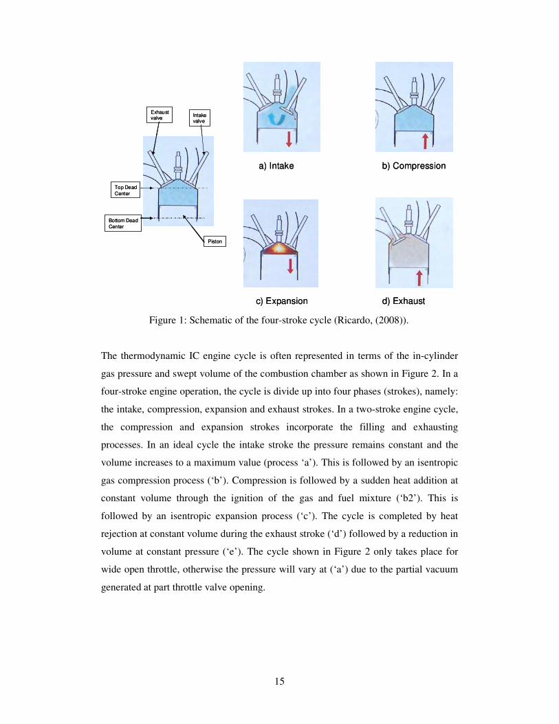
The thermodynamic IC engine cycle is often represented in terms of the in-cylinder
gas pressure and swept volume of the combustion chamber as shown in Figure 2. In a
four-stroke engine operation, the cycle is divide up into four phases (strokes), namely:
the intake, compression, expansion and exhaust strokes. In a two-stroke engine cycle,
the compression and expansion strokes incorporate the filling and exhausting
processes. In an ideal cycle the intake stroke the pressure remains constant and the
volume increases to a maximum value (process ‘a’). This is followed by an isentropic
gas compression process (‘b’). Compression is followed by a sudden heat addition at
constant volume through the ignition of the gas and fuel mixture (‘b2’). This is
followed by an isentropic expansion process (‘c’). The cycle is completed by heat
rejection at constant volume during the exhaust stroke (‘d’) followed by a reduction in
volume at constant pressure (‘e’). The cycle shown in Figure 2 only takes place for
wide open throttle, otherwise the pressure will vary at (‘a’) due to the partial vacuum
generated at part throttle valve opening.
a) Intake b) Compression
c) Expansion d) Exhaust
Intakevalve
Exhaustvalve
Top Dead
Center
Bottom Dead
Center
Piston
a) Intake b) Compression
c) Expansion d) Exhaust
Intakevalve
Exhaustvalve
Top Dead
Center
Bottom Dead
Center
Piston
16
Figure 2: Real pressure-volume diagrams for four-stroke and two-stroke poppet valve
engines respectively.
Figure 3 shows the in-cylinder pressure against Crank Angle (CA) position of the
piston. In the case of four-stroke engines the cycle takes seven hundred and twenty
degrees (two rotations) to complete. Two-stroke engines only take half the time (one
a, e
b
b2 c
d
P-V diagram two-stroke
-10
0
10
20
30
40
50
60
70
80
0 0.0002 0.0004 0.0006 0.0008 0.001 0.0012 0.0014
V (m3)
P (
bar)
P
a, e
b
b2 c
d
a, e
b
b2 c
d
P-V diagram two-stroke
-10
0
10
20
30
40
50
60
70
80
0 0.0002 0.0004 0.0006 0.0008 0.001 0.0012 0.0014
V (m3)
P (
bar)
P
a
b
b2 c
d
e
P-V diagram four-stroke
-10
0
10
20
30
40
50
60
70
80
0 0.0002 0.0004 0.0006 0.0008 0.001 0.0012 0.0014
V (m3)
P (
ba
r)
P
a
b
b2 c
d
e
a
b
b2 c
d
e
P-V diagram four-stroke
-10
0
10
20
30
40
50
60
70
80
0 0.0002 0.0004 0.0006 0.0008 0.001 0.0012 0.0014
V (m3)
P (
ba
r)
P
17
rotation) to complete the whole cycle. This means that the specific power output could
be double that of the four-stroke engine cycle. However in practical applications, the
friction, noise, heat losses generated increase and the gas exchange process is not
ideal.
In the two-stroke cycle the exhaust and intake strokes take place together such that the
gas exchange process differs from that in the four-stroke engine. In Figure 3 the two-
stroke (2s) instantaneous pressure are shown in blue colour, while the four-stroke (4s)
ones are shown in brown. Also the four- and two-stroke valve timings are shown on
the top and bottom part of the figure respectively. The timings clearly show the
increased scavenging period required in two-stroke engines over four-stroke ones to
maximise the air flow in and out of the combustion chamber.
Figure 3: Example of pressure-crank angle diagram for four-stroke and two-stroke
engines including valve events (typical).
One of the main differences between four-stroke and two-stroke engines is in their
mechanical design. Traditionally two-stroke engines have been of a piston ported
design as shown in Figure 4, where the piston transfers the mechanical work to the
crankshaft in a similar way to four-stroke engines. In two-stroke engines the piston
also behaves as a valve, separating chambers. The two-stroke piston ported engines
Four- and two-stroke pressure-crank angle diagram
-10
0
10
20
30
40
50
60
70
80
-360 -280 -200 -120 -40 40 120 200 280 360
CA
P (
bar) P four-stroke
P two-stroke
4S IVO4S IVC4S EVC 4S EVO
2S EVO 2S EVC 2S EVO 2S EVC
2S IVO 2S IVO2S IVC 2S IVC

18
more simplistic design, together with the scavenging needs, and increased emission
levels in comparison to four-stroke engines, have generally limited their use to
motorcycles and small appliance engines. However, this does not mean that two-
stroke engines may not be of a poppet valve design. This will require different valve
timings in which the inlet and exhaust valves are open simultaneously for a certain
period of time, to promote an improved scavenge process through the exhaust and
intake stroke as shown in Figure 5. This requires accurate timing to avoid fresh air
escaping into the exhaust port, thereby reducing the engine efficiency (short-cutting).
An increase in engine boost is also needed to push the gases in and out of the engine
as required and to avoid engine knock effects due to poor scavenge.
Figure 4: Example of schematic of physical two-stroke piston ported engine design
(Heywood, (1988)).
Transferport
Piston
deflectorExhaust
port
b) Compression & Expansion
Inlet
port
Transfer
port
Pistondeflector
Exhaustport
a) Intake & Exhaust
Inlet
port
Transferport
Piston
deflectorExhaust
port
b) Compression & Expansion
Inlet
port
Transferport
Piston
deflectorExhaust
port
b) Compression & Expansion
Inlet
port
Transfer
port
Pistondeflector
Exhaustport
a) Intake & Exhaust
Inlet
port
Transfer
port
Pistondeflector
Exhaustport
a) Intake & Exhaust
Inlet
port
19
Figure 5: Principle characteristics of two-stroke ported engines (Ricardo, (2008)).
In the case of an ideal cycle the process has no losses and is also considered
reversible. In a real IC engine, the Carnot Efficiency or Thermal Efficiency is given
by Eq.2.1-1.
1
2
1 111
−−=−=
γη
cs
s
thrT
T 2.1-1
where v
p
c
c=γ
where Ts1 is the temperature into the system from the surroundings, Ts2 is the peak
engine temperature, rc is the compression ratio, cv is the specific heat at constant
volume, cp is the specific heat at constant pressure and γ (Gamma) is the ratio of
specific heats.
In Eq.2.1-1, the efficiency may be improved by increasing the compression ratio,
although this is limited by mixture auto-ignition and mechanical constraints. Gamma
is considered equal to 1.4 for ideal gases, although in IC engine its value varies from
Intakevalve
Exhaustvalve
Top Dead
Center
Bottom DeadCenter
Piston
b) Compression
c) Expansion d) Exhaust
a) Intake
Intakevalve
Exhaustvalve
Top Dead
Center
Bottom DeadCenter
Piston
b) Compression
c) Expansion d) Exhaust
a) Intake
20
1.2-1.5, hence increasing it will also increase the engine efficiency, besides the leaner
a mixture is the higher the value of Gamma is, this together with low combustion
temperature situations increases the efficiency, because Gamma is a function of the
Air to Fuel Ratio (AFR) and Temperature (Cardosa, (2009)).
The real IC engine cycle is far from an ideal process. This is due to several facts such
as:
• The gas mixture is far from ideal as the value of Gamma, γ suggests (Eq.2.1-1)
• The combustion process is not considered
• None of the processes in the cycle are instantaneous
• The ignition timing is varied with the engine speed and load
• Friction and heat losses to the chamber walls and to the exhaust gases are
present
• Blow-by of gases takes place during the cycle
• There are pumping losses to get fresh combustion charge in and exhaust gases
out of the chamber
• Engine and ancillary components create additional friction losses
• Noise and vibration are other sources of inefficiency
Determination of the heat release from the combustion chamber is of particular
importance in estimating the efficiency. To obtain this, an engine energy balance
system is devised as shown in Figure 6. From the first law of thermodynamics, the
change in addition of energy, less the outgoing energy and the internal energy, is
always equal to zero as Eq.2.1-2.
21
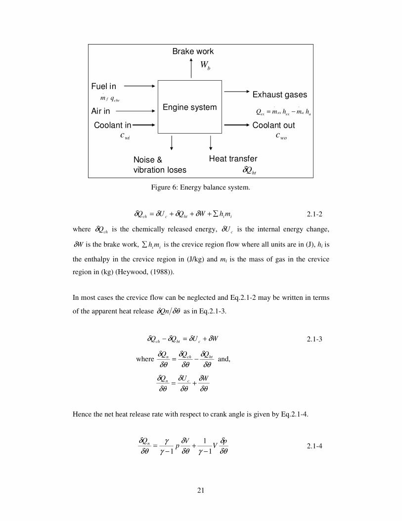
Figure 6: Energy balance system.
iihtcch mhWQUQ ∑+++= δδδδ 2.1-2
where chQδ is the chemically released energy, cUδ is the internal energy change,
Wδ is the brake work, ii mh∑ is the crevice region flow where all units are in (J), hi is
the enthalpy in the crevice region in (J/kg) and mi is the mass of gas in the crevice
region in (kg) (Heywood, (1988)).
In most cases the crevice flow can be neglected and Eq.2.1-2 may be written in terms
of the apparent heat release δθδQn as in Eq.2.1-3.
WUQQ chtch δδδδ +=− 2.1-3
where δθ
δ
δθ
δ
δθ
δ htchn QQQ−= and,
δθ
δ
δθ
δ
δθ
δ WUQ cn +=
Hence the net heat release rate with respect to crank angle is given by Eq.2.1-4.
δθ
δ
γδθ
δ
γ
γ
δθ
δ pV
Vp
Qn
1
1
1 −+
−= 2.1-4
Engine system
Fuel in
Brake work
Air in
Exhaust gases
Noise &
vibration loses
chvf qm.
bW
wic wocCoolant in Coolant out
Heat transfer
aaexexex hmhmQ..
−=
htQδ
Engine system
Fuel in
Brake work
Air in
Exhaust gases
Noise &
vibration loses
chvf qm.
bW
wic wocCoolant in Coolant out
Heat transfer
aaexexex hmhmQ..
−=
htQδ
22
The value of γ in Eq. 2.1-4 may be obtained from the polytropic gas relationship in
Eq.2.1-5. This approximates well the compression and expansion processes (“b” and
“c” in Figure 2 respectively). Note the value of γ is higher in compression stroke
because of the heat losses during expansion.
constpV =γ 2.1-5
where p is the chamber pressure and V is the volume.
The heat transfer term includes contributions due to convection, conduction and
radiation.
A. The heat transfer term htQδ in Eq.2.1-2 includes heat losses to the engine metal
surfaces and into the coolant. This is derived from “Newton’s Law” of cooling or
convection in Eq.2.1-6:
( )wmi
ht TThAt
Q−=
δ
δ 2.1-6
where Ai is the instantaneous combustion chamber area, h is the heat transfer
coefficient, Tm is the mean gas temperature and Tw is the combustion chamber mean
wall temperature.
Since the instantaneous local gas temperature combustion chamber Tg is not possible
to measure mean values, Tm are considered instead. The value of Ai may be calculated
by the following expression, Eq.2.1-7.
( )( )( )2122
1
2
11 sincos θθπ alaaldAAA cpchi −+−+++= 2.1-7
where Ach is the combustion chamber area at TDC, Acp is the piston area, l is the
connecting rod length and a1 is half of the stroke length.
The heat transfer htQδ can also be derived when the amount of fuel supplied to the
engine is known, as well as the calorific value, and therefore obtaining the energy
supplied to the engine. Since the crevices are neglected, htQδ is obtained from
Eq.2.1-4. The values of htQδ have been reported up to ten to fifteen percent higher
23
than measured values, but they still provide an important estimation of engine heat
release (Heywood, (1988)).
B. The heat transfer by conduction through the chamber walls is derived by the
temperature drop in the metal through the wall Eq.2.1-8.
k
Q
dx
dT w= 2.1-8
where Qw is the heat flux at the combustion chamber wall.
C. Thermal radiation, Qrad present in the combustion chamber is given by Eq.2.1-9
( ) ( )[ ]44
0 wgrad TTQ −= σε 2.1-9
where εo is the emissivity coefficient in dimensionless form and σ is the Stefan-
Boltzmann constant equal to 5.6.10
-8 W/m
2K
4.
For a similar engine capacity, two-stroke operation (Figure 3) generates
approximately double the amount of heat flux than four-stroke operation (specific
power output). However, the four-stroke part-load fuel consumption is lower. Hence a
combination of the optimum capabilities of both two- and four-stroke engines is of
particular interest. This feature, together with emerging camshaft timing technologies,
has managed to combine both four- and two-stroke engines together in the same
poppet valve engine design, thus improving performance and emissions. This has
enabled both operating modes to be investigated under the same conditions and
compared accurately. Eventually this may give advantages in passenger cars such as
engine size reduction (downsizing), increased output and improved economy. The
higher demands for engine thermal load is initially addressed by upgrading the engine
cooling design to work safely during both two- and four-stroke operations. However
the engine thermal behaviour needs to be analysed in more depth, as potentially there
is a possibility of damaging the cylinder head, during full torque, two-stroke, cycle
operation.
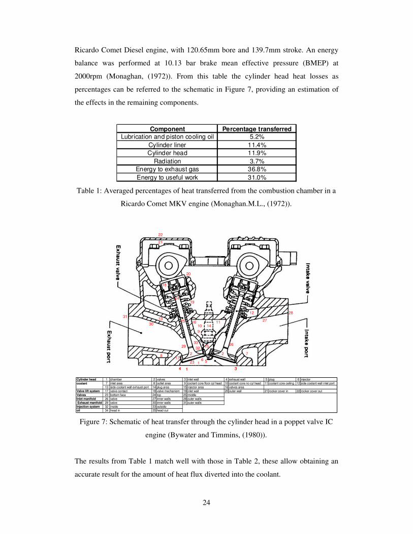
Typical heat losses in a Diesel engine are shown in Table 1, quantifying the heat
distribution in different engine regions. The experiment was performed using a
24
Ricardo Comet Diesel engine, with 120.65mm bore and 139.7mm stroke. An energy
balance was performed at 10.13 bar brake mean effective pressure (BMEP) at
2000rpm (Monaghan, (1972)). From this table the cylinder head heat losses as
percentages can be referred to the schematic in Figure 7, providing an estimation of
the effects in the remaining components.
Table 1: Averaged percentages of heat transferred from the combustion chamber in a
Ricardo Comet MKV engine (Monaghan.M.L., (1972)).
Figure 7: Schematic of heat transfer through the cylinder head in a poppet valve IC
engine (Bywater and Timmins, (1980)).
The results from Table 1 match well with those in Table 2, these allow obtaining an
accurate result for the amount of heat flux diverted into the coolant.
1
2 2
34
56
78
9
1011
12
13
14
15
16
17
18
19
20
21
22
23
24
25
1
26
27
28
29
30
31
32
33
1
2 2
34
56
78
9
1011
12
13
14
15
16
17
18
19
20
21
22
23
24
25
1
26
27
28
29
30
31
32
33
1 chamber 2 valves 3 inlet wall 4 exhaust wall 5 plug 6 injector
7 inlet area 8 outlet area 9 coolant core floor cyl head 10 coolant core no cyl head 11 coolant core ceiling 12 side coolant wall inlet port
13 side coolant wall exhaust port 14 plug area 15 injector area 16 valves area
17 valve contact 18 valve mechanism 19 inlet wall 20 outer wall 21 rocker cover in 22 rocker cover out
23 bottom face 24 top 25 middle
26 valve 27 inner walls 28 outer walls
29 valve 30 inner walls 31 outer walls
32 inside 33 outside
34 head in 35 head out
Cylinder head
coolant
Valve lift system
Valves
Inlet manifold
Exhaust manifold
Injection system
oil
Component Percentage transferredLubrication and piston cooling oil 5.2%
Cylinder liner 11.4%
Cylinder head 11.9%
Radiation 3.7%
Energy to exhaust gas 36.8%
Energy to useful work 31.0%

25
Table 2: Energy balance at maximum power (Heywood, (1988)).
2.2 Description of the research problem;
An IC engine real cycle is far from a steady-state process. In particular, the thermal
loading varies considerably depending on the cycle used, engine design and the
operating conditions. If it is not controlled suitably the situation may lead to reduced
performance and fuel economy, fatigue, crack propagation and failure. Since heat
energy contributes to all of these problems, quantifying it is of maximum importance.
In the engine environment, the time varying working conditions (volume, gas
pressure-temperature and local gas velocities) are rapid when compared to the slow
rate of change in mean heat flux through the metal that can be experimentally
measured. Estimated values or approximations are derived in the system through
applying the energy balance. For these reasons IC engine thermal studies generally
are of two different kinds.
• Local heat flux studies; where a thermal map over the combustion chamber
surface is obtained from (near) instantaneous local measured values.
• Mean heat flux studies; where time-averaged measurements are taken and
averaged over the entire combustion chamber surface.
Local results provide a more accurate description of the situation; however the
procedure is impractical in creating a fully thermally controlled engine. A source of
errors, are the limits of the measuring devices with a typical time response of a second
and an error of ±1oC.
In the proposed investigation, it is important to understand what types of heat transfer
will occur and which ones are most relevant. These are listed as follows:
• Forced convection heat transfer in the combustion chamber amounts to
approximately 75-80% of the total heat released in IC engines. The maximum
value occurs at approximately 30-40ºCA after ignitions starts, during the
expansion stroke for a spark ignition engine. Since the volume at TDC is small
when the maximum heat release occurs, most of this heat energy is transferred
25-28% 17-26% 3-10% 2-5% 34-45%
Exhaust
enthalpy
Brake
power
Heat flux
to coolant
Q rejected to oil
and atmosphere
Chemical enthalpy flux
incomplete combustion

26
to the chamber walls before 55ºCA after TDC (Annand, (1962)). Forced
convection heat transfer may be calculated by Eq.2.1-6.
• Radiation heat transfer is also present through the air-fuel burning process. It’s
value can be estimated by Eq.2.1-9. However since the time taken in the
burning process is so small, it is normally considered an instantaneous
reaction. Hence some mathematical models neglect it or a simple correction
value is applied.
• Conduction is present through the metal material only. The temperature
carried through the wall may be calculated by Eq.2.1-8.
The heat transfer modes described are schematically shown in terms of temperature
distribution in Figure 8.
Figure 8: Temperature distribution diagram.
where Tw,c is the coolant side wall temperature and Tcm is the mean coolant
temperature.
In most cases dimensional analysis is used to obtain an expression for heat transfer
from the gas side. One Dimensional (1-D) heat flow is considered to move parallel to
the piston axis through the cylinder head, although this may not be valid in more
realistic situations.
The final outcome in any combustion chamber thermal study will be obtaining the
heat flux from the combustion chamber to the metal surface. In some empirical
studies, the heat flux has been obtained with reasonable accuracy however, since the
Temp(K)
Tg
Tm
Tw
Tw, c
Tc
Tcm
Gas side(convection,radiation)
Coolant side(convection)
Wall(conduction)
Distance
Temp(K)
Tg
Tm
Tw
Tw, c
Tc
Tcm
Gas side(convection,radiation)
Coolant side(convection)
Wall(conduction)
Distance
27
combustion chamber temperature distribution cannot always be reliably determined, it
is often more reliable to calculate the heat transfer coefficient. Through the use of 1-D
models, simple and accurate calculations can be obtained. These have been classified
as follows:
• Instantaneous heat flux averaged over the chamber surface: the temperature
values are specified at each time or CA position. They are considered
averaged at any place in the volume.
• Local instantaneous heat flux over the surface: the temperature values are
specified at each time or CA position. These are varied over the area
considered, thus creating a thermal map.
• Average heat flux results through time: the results are averaged over a time or
CA range and the remaining swept volume. This provide an energy balance
similar to the one used to analyze engine efficiencies (Borman and Nishiwaki,
(1987)).
All of the 1-D models in the literature are based upon either “Newton’s Law”
or“Nusselt Analogy”. “Newton’s law” (including conduction, convection and
radiation terms) has been given previously in Eq.2.1-8, Eq.2.1-6 and Eq.2.1-9
respectively.
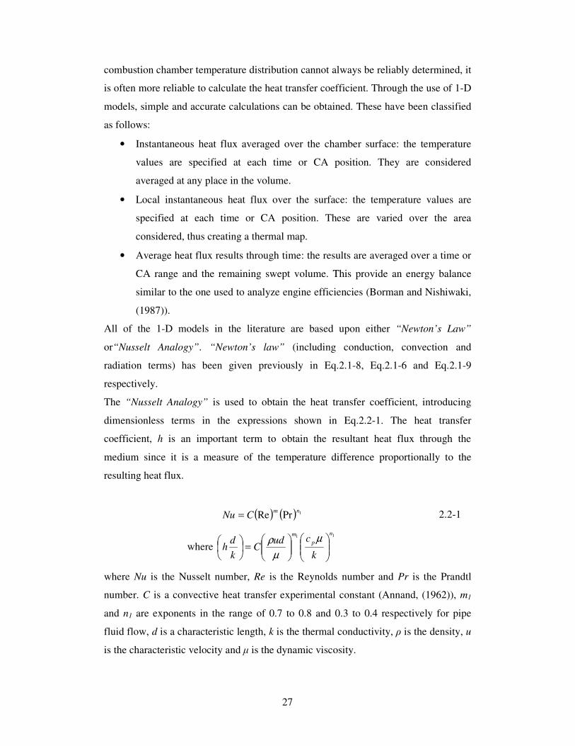
The “Nusselt Analogy” is used to obtain the heat transfer coefficient, introducing
dimensionless terms in the expressions shown in Eq.2.2-1. The heat transfer
coefficient, h is an important term to obtain the resultant heat flux through the
medium since it is a measure of the temperature difference proportionally to the
resulting heat flux.
( ) ( ) 1PrRenm
CNu = 2.2-1
where
11n
p
m
k
cudC
k
dh
=
µ
µ
ρ
where Nu is the Nusselt number, Re is the Reynolds number and Pr is the Prandtl
number. C is a convective heat transfer experimental constant (Annand, (1962)), m1
and n1 are exponents in the range of 0.7 to 0.8 and 0.3 to 0.4 respectively for pipe
fluid flow, d is a characteristic length, k is the thermal conductivity, ρ is the density, u
is the characteristic velocity and µ is the dynamic viscosity.
28
The Nusselt number is a measure of the heat exchange between the gas and the wall
through conduction and convection effects. The Reynolds number characterises the
turbulent or laminar flow regime along the medium and the Prandtl number relates the
rate of fluid transport in a stream to its diffusion rate. In free convection situations
Reynolds and Prandtl numbers may be neglected.
In situations where the heat flows from fluid to solids, Newton’s Law of cooling can
be applied (Eq.2.1-6) to cases of both free and forced convection.
2.3 Dimensional analysis and empirical correlation
Experimental correlations can be classified by either heat flux or heat transfer
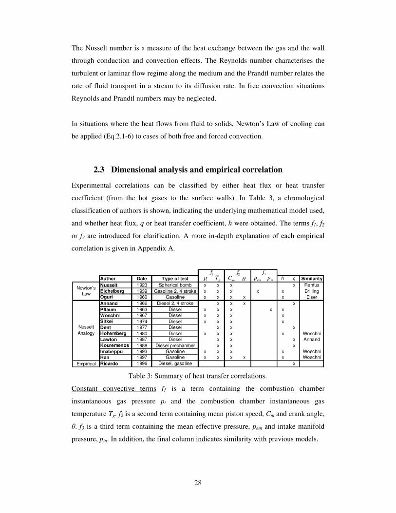
coefficient (from the hot gases to the surface walls). In Table 3, a chronological
classification of authors is shown, indicating the underlying mathematical model used,
and whether heat flux, q or heat transfer coefficient, h were obtained. The terms f1, f2
or f3 are introduced for clarification. A more in-depth explanation of each empirical
correlation is given in Appendix A.
Table 3: Summary of heat transfer correlations.
Constant convective terms f1 is a term containing the combustion chamber
instantaneous gas pressure pi and the combustion chamber instantaneous gas
temperature Tg. f2 is a second term containing mean piston speed, Cm and crank angle,
θ. f3 is a third term containing the mean effective pressure, pem and intake manifold
pressure, pin. In addition, the final column indicates similarity with previous models.
Author Date Type of test h q Similarity
Nusselt 1923 Spherical bomb x x x x Rehfus
Eichelberg 1939 Gasoline 2, 4 stroke x x x x x BrillingOguri 1960 Gasoline x x x x x Elser
Annand 1962 Diesel 2, 4 stroke x x x x
Pflaum 1963 Diesel x x x x x
Woschni 1967 Diesel x x x x
Sitkei 1974 Diesel x x x x
Dent 1977 Diesel x x x
Hohemberg 1980 Diesel x x x x Woschni
Lawton 1987 Diesel x x x Annand
Kouremenos 1988 Diesel prechamber x x x
Imabeppu 1993 Gasoline x x x x Woschni
Han 1997 Gasoline x x x x x Woschni
Empirical Ricardo 1996 Diesel, gasoline x
Newton's
Law
Nusselt
Analogy
ip
gT
mC θ em
pin
p1f 2f 3f
29
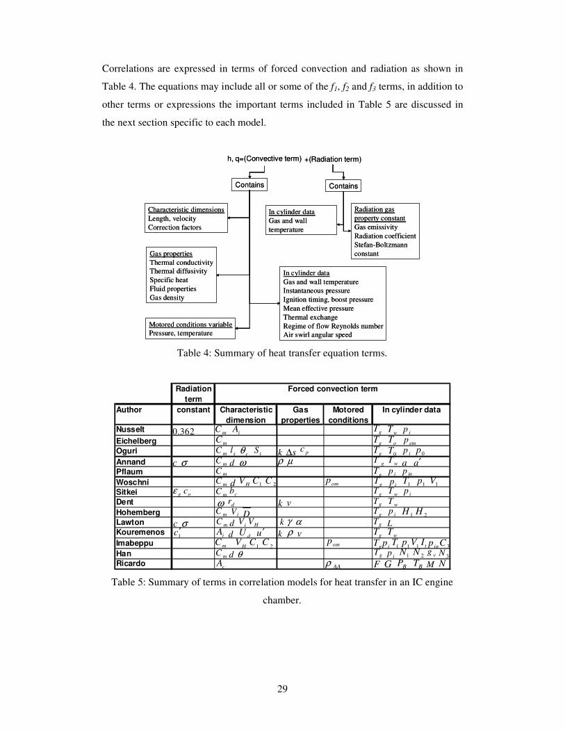
Correlations are expressed in terms of forced convection and radiation as shown in
Table 4. The equations may include all or some of the f1, f2 and f3 terms, in addition to
other terms or expressions the important terms included in Table 5 are discussed in
the next section specific to each model.
Table 4: Summary of heat transfer equation terms.
Table 5: Summary of terms in correlation models for heat transfer in an IC engine
chamber.
Nusselt
Eichelberg
Oguri
Annand
Pflaum
Woschni
Sitkei
Dent
Hohemberg
Lawton
Kouremenos
Imabeppu
Han
Ricardo
Forced convection term
constant Characteristic
dimension
Radiation
term
Motored
conditions
Gas
properties
Author In cylinder data
iA
iA
mC
mC
mC
mC
mC
mC
mC
mC
mC
tSsl
θ
d
d HV 1C 2C
cb
ω
dU u′
cA
k
k
k v
v
AAρ
gT
gT
gT
gT
gT
gT
gT
gT
ip
ip
ip
ip
ip
wT
wT
wT
wT
oT
inp
1T 1p 1V
1H 2H
tI3C
F G BP BT1N
362.0
gε oc
1c′
ip
emp
gT
gT
s∆ρ µ a a′ωc σ
ip
wT
iV HViV
γmC dc σd
dip1
CmC2
CH
V
2N vg
gT
3N
gT
1T
1p
1V
gTk ρ
inp
rθ
dr
D
pc
α
omp
omp
0T 0p
L
M N
h, q=(Convective term)
In cylinder data
Gas and wall temperature
Instantaneous pressure
Ignition timing, boost pressure
Mean effective pressure
Thermal exchange
Regime of flow Reynolds number
Air swirl angular speed
Contains
Gas properties
Thermal conductivity
Thermal diffusivity
Specific heat
Fluid properties
Gas density
Characteristic dimensions
Length, velocity
Correction factors
Motored conditions variable
Pressure, temperature
+(Radiation term)
Contains
In cylinder data
Gas and wall
temperature
Radiation gas
property constant
Gas emissivity
Radiation coefficient
Stefan-Boltzmann
constant
30
2.4 Empirical heat transfer coefficient correlations
In the following section, a summary of the correlations is presented. A full description
is given in Appendix A. Empirical models have been derived by consideration of the
general terms in Table 4 with experimental results.
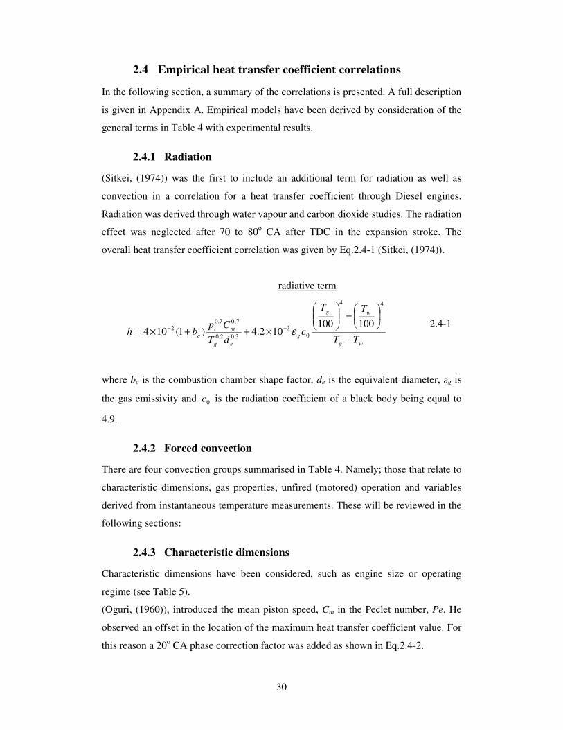
2.4.1 Radiation
(Sitkei, (1974)) was the first to include an additional term for radiation as well as
convection in a correlation for a heat transfer coefficient through Diesel engines.
Radiation was derived through water vapour and carbon dioxide studies. The radiation
effect was neglected after 70 to 80o CA after TDC in the expansion stroke. The
overall heat transfer coefficient correlation was given by Eq.2.4-1 (Sitkei, (1974)).
radiative term
wg
wg
g
eg
mi
cTT
TT
cdT
Cpbh
−
−
×++×= −−
44
0
3
3.02.0
7,07.0
2100100
102.4)1(104 ε 2.4-1
where bc is the combustion chamber shape factor, de is the equivalent diameter, εg is
the gas emissivity and 0c is the radiation coefficient of a black body being equal to
4.9.
2.4.2 Forced convection
There are four convection groups summarised in Table 4. Namely; those that relate to
characteristic dimensions, gas properties, unfired (motored) operation and variables
derived from instantaneous temperature measurements. These will be reviewed in the
following sections:
2.4.3 Characteristic dimensions
Characteristic dimensions have been considered, such as engine size or operating
regime (see Table 5).
(Oguri, (1960)), introduced the mean piston speed, Cm in the Peclet number, Pe. He
observed an offset in the location of the maximum heat transfer coefficient value. For
this reason a 20o CA phase correction factor was added as shown in Eq.2.4-2.
31
( )( )°−+
∆+= 20cos2175.1 r
pc
s
Pe
Nuθ 2.4-2
where α
mdCPe = and,
( )
−−
=
∆
00
ln1
lnp
p
k
k
T
T
c
s ig
p
and,
PrRe=Pe
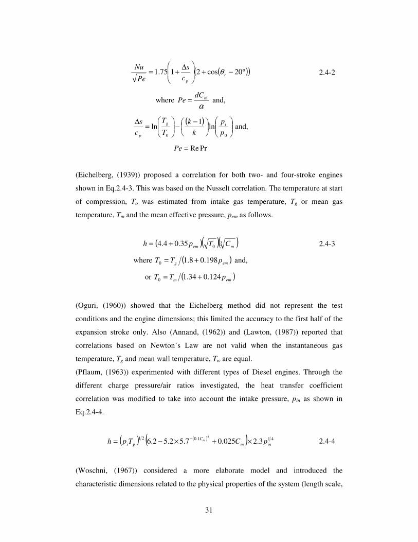
(Eichelberg, (1939)) proposed a correlation for both two- and four-stroke engines
shown in Eq.2.4-3. This was based on the Nusselt correlation. The temperature at start
of compression, To was estimated from intake gas temperature, Tg or mean gas
temperature, Tm and the mean effective pressure, pem as follows.
( )( )( )3035.04.4 mem CTph += 2.4-3
where ( )emg pTT 198.08.10 += and,
or ( )emm pTT 124.034.10 +=
(Oguri, (1960)) showed that the Eichelberg method did not represent the test
conditions and the engine dimensions; this limited the accuracy to the first half of the
expansion stroke only. Also (Annand, (1962)) and (Lawton, (1987)) reported that
correlations based on Newton’s Law are not valid when the instantaneous gas
temperature, Tg and mean wall temperature, Tw are equal.
(Pflaum, (1963)) experimented with different types of Diesel engines. Through the
different charge pressure/air ratios investigated, the heat transfer coefficient
correlation was modified to take into account the intake pressure, pin as shown in
Eq.2.4-4.
( ) ( )( ) 411.0213.2025.07.52.52.6
2
inm
C
gi pCTph m ×+×−= − 2.4-4
(Woschni, (1967)) considered a more elaborate model and introduced the
characteristic dimensions related to the physical properties of the system (length scale,
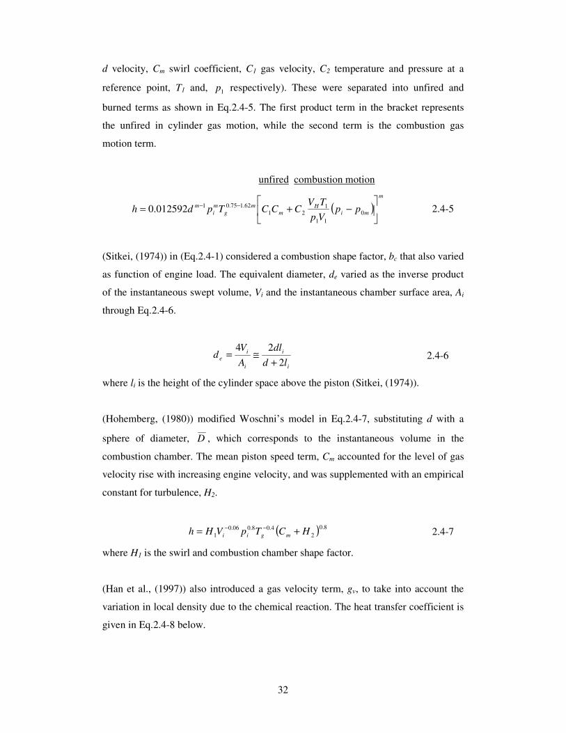
32
d velocity, Cm swirl coefficient, C1 gas velocity, C2 temperature and pressure at a
reference point, T1 and, 1p respectively). These were separated into unfired and
burned terms as shown in Eq.2.4-5. The first product term in the bracket represents
the unfired in cylinder gas motion, while the second term is the combustion gas
motion term.
unfired combustion motion
( )m
mi
H
m
m
g
m
i
mpp
Vp
TVCCCTpdh
−+= −−
0
11
121
62.175.01012592.0 2.4-5
(Sitkei, (1974)) in (Eq.2.4-1) considered a combustion shape factor, bc that also varied
as function of engine load. The equivalent diameter, de varied as the inverse product
of the instantaneous swept volume, Vi and the instantaneous chamber surface area, Ai
through Eq.2.4-6.
i
i
i
i
eld
dl
A
Vd
2
24
+≅= 2.4-6
where li is the height of the cylinder space above the piston (Sitkei, (1974)).
(Hohemberg, (1980)) modified Woschni’s model in Eq.2.4-7, substituting d with a
sphere of diameter, D , which corresponds to the instantaneous volume in the
combustion chamber. The mean piston speed term, Cm accounted for the level of gas
velocity rise with increasing engine velocity, and was supplemented with an empirical
constant for turbulence, H2.
( ) 8.0
2
4.08.006.0
1 HCTpVHh mgii += −− 2.4-7
where H1 is the swirl and combustion chamber shape factor.
(Han et al., (1997)) also introduced a gas velocity term, gv, to take into account the
variation in local density due to the chemical reaction. The heat transfer coefficient is
given in Eq.2.4-8 below.
33
75.0
32
465.075.025.0
1
35.1
++=
−−
δθδθivvi
mgi
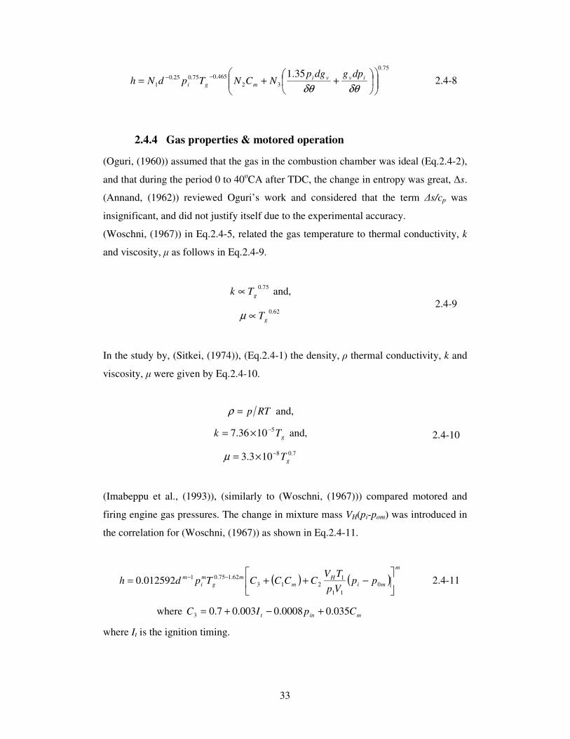
dpgdgpNCNTpdNh 2.4-8
2.4.4 Gas properties & motored operation
(Oguri, (1960)) assumed that the gas in the combustion chamber was ideal (Eq.2.4-2),
and that during the period 0 to 40oCA after TDC, the change in entropy was great, ∆s.
(Annand, (1962)) reviewed Oguri’s work and considered that the term ∆s/cp was
insignificant, and did not justify itself due to the experimental accuracy.
(Woschni, (1967)) in Eq.2.4-5, related the gas temperature to thermal conductivity, k
and viscosity, µ as follows in Eq.2.4-9.
75.0
gTk ∝ and,
62.0
gT∝µ
2.4-9
In the study by, (Sitkei, (1974)), (Eq.2.4-1) the density, ρ thermal conductivity, k and
viscosity, µ were given by Eq.2.4-10.
RTp=ρ and,
gTk51036.7 −×= and,
7.08103.3 gT−×=µ
2.4-10
(Imabeppu et al., (1993)), (similarly to (Woschni, (1967))) compared motored and
firing engine gas pressures. The change in mixture mass VH(pi-pom) was introduced in
the correlation for (Woschni, (1967)) as shown in Eq.2.4-11.
( ) ( )m
miH
m
m
g
m
i
mpp
Vp
TVCCCCTpdh
−++= −−
0
11
1213
62.175.01012592.0 2.4-11
where mint CpIC 035.00008.0003.07.03 +−+=
where It is the ignition timing.
34
2.4.5 Instantaneous temperature measured values
(Eichelberg, (1939)) in (Eq.2.4-3), considered the mean effective pressure, pem, to
correct the temperature at the start of compression, To.
(Pflaum, (1963)) assumed that since the heat transfer is only sufficiently high only
from the end of compression- up to the beginning of the exhaust-stroke, he considered
that correlations based upon characteristic length terms and instantaneously measured
results were not sufficient, since they were missing an intake pressure, pin term as
shown in Eq.2.4-4.
(Woschni, (1967)) through Eq.2.4-5 suggested that the instantaneous pressure, pi and
the instantaneous gas temperature, Tg should be aided by a combustion motion term,
formed by a motored and fired pressure difference.
(Sitkei, (1974)) in Eq.2.4-1 made the instantaneous pressure, pi and the instantaneous
gas temperature, Tg, dependant upon the combustion shape factor.
(Hohemberg, (1980)) made Woschni’s combustion turbulence flow velocity term to
be affected by H2 only. The instantaneous gas temperature Tg exponent was modified
since the heat transfer coefficient, h variation is directly proportional to the
instantaneous pressure, pi and inversely proportional to Tg as shown in Eq.2.4-7.
(Imabeppu et al., (1993)) modified Woschni flow velocity term through the correction
factor, C3 to obtain the overall heat transfer coefficient, h instead of the local one
through Eq.2.4-11, this would implement a corrected result for the inconsistent
coolant heat rejection.
2.5 Empirical heat flux correlations
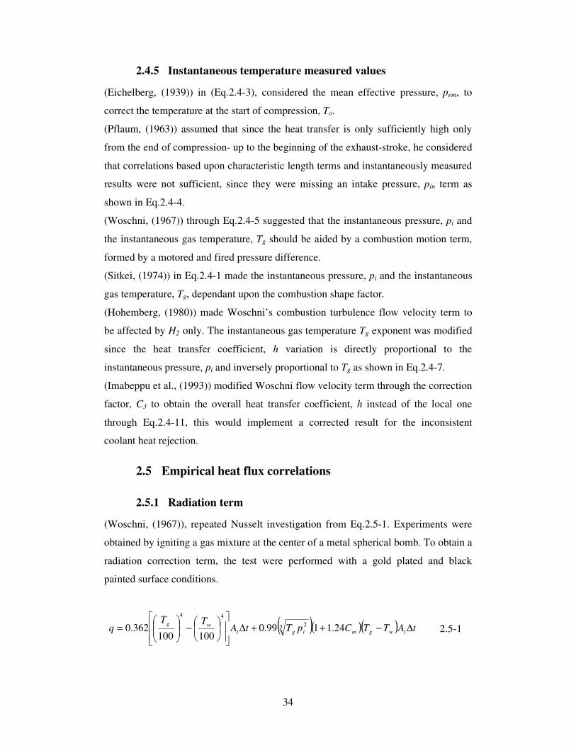
2.5.1 Radiation term
(Woschni, (1967)), repeated Nusselt investigation from Eq.2.5-1. Experiments were
obtained by igniting a gas mixture at the center of a metal spherical bomb. To obtain a
radiation correction term, the test were performed with a gold plated and black
painted surface conditions.
( )( )( ) tATTCpTtATT
q iwgmigi
wg∆−++∆
−
= 24.1199.0
100100362.0 3 2
44
2.5-1

35
(Annand and Ma, (1972)) through Diesel engine studies in both two- and four-stroke
configuration derived Eq.2.5-2.
( ) ( )44'
Re wg
g
wg
bTTc
t
TaTTa
d
kq −+
+−
= σ
δ
δ
ω 2.5-2
where a’ is the mean gas temperature coefficient.
(Lawton, (1987)) through his Diesel experiments upgraded Annand correlation
through Eq.2.5-3.
( )[ ] ( )447.0 75.2Re28.0 wgwwg TTcLTTTd
kq −+−−= σ 2.5-3
Where term ( )m
i
C
d
V
VL
αγ
3
1−=
where α is the thermal diffusivity and L is the compressibility number.
(Annand, (1962)) through Eq.2.5-2 and (Lawton, (1987)) Eq.2.5-3 considered the
Stefan-Boltzmann constant and an experimental combustion and expansion strokes
correction factor.
(Kouremenos et al., (1988)) through pre-chamber Diesel engine studies, derived a
radiation heat flux term only valid in the combustion chamber and a different
radiation coefficient, c’ through Eq.2.5-4.
( ) ( )[ ]44
gwgwi TTcTThAq +′+−= 2.5-4
where 33.0
8.022
33.08.0 Pr037.0
PrRe037.0
′+==
υ
ρ uUd
d
k
d
kh
d
(Dent and Suliaman, (1977)) during their high swirl Diesel engine experiments in
motoring and fired conditions, did not observed any radiation and derived Eq.2.5-5.
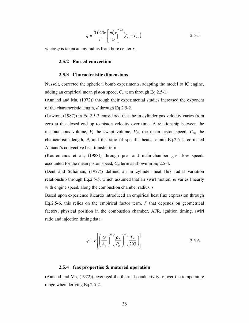
36
( )wrg
s TTr
r
kq −
=
8.02
023.0
υ
ω 2.5-5
where q is taken at any radius from bore center r.
2.5.2 Forced convection
2.5.3 Characteristic dimensions
Nusselt, corrected the spherical bomb experiments, adapting the model to IC engine,
adding an empirical mean piston speed, Cm term through Eq.2.5-1.
(Annand and Ma, (1972)) through their experimental studies increased the exponent
of the characteristic length, d through Eq.2.5-2.
(Lawton, (1987)) in Eq.2.5-3 considered that the in cylinder gas velocity varies from
zero at the closed end up to piston velocity over time. A relationship between the
instantaneous volume, Vi the swept volume, VH, the mean piston speed, Cm, the
characteristic length, d, and the ratio of specific heats, γ into Eq.2.5-2, corrected
Annand’s convective heat transfer term.
(Kouremenos et al., (1988)) through pre- and main-chamber gas flow speeds
accounted for the mean piston speed, Cm term as shown in Eq.2.5-4.
(Dent and Suliaman, (1977)) defined an in cylinder heat flux radial variation
relationship through Eq.2.5-5, which assumed that air swirl motion, ω varies linearly
with engine speed, along the combustion chamber radius, r.
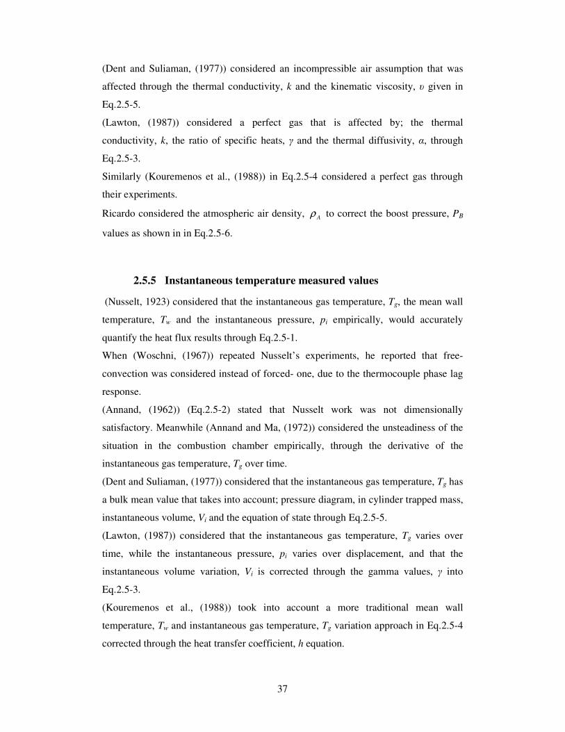
Based upon experience Ricardo introduced an empirical heat flux expression through
Eq.2.5-6, this relies on the empirical factor term, F that depends on geometrical
factors, physical position in the combustion chamber, AFR, ignition timing, swirl
ratio and injection timing data.
=
293
B
N
B
A
M
c
T
PA
GFq
ρ 2.5-6
2.5.4 Gas properties & motored operation
(Annand and Ma, (1972)), averaged the thermal conductivity, k over the temperature
range when deriving Eq.2.5-2.
37
(Dent and Suliaman, (1977)) considered an incompressible air assumption that was
affected through the thermal conductivity, k and the kinematic viscosity, υ given in
Eq.2.5-5.
(Lawton, (1987)) considered a perfect gas that is affected by; the thermal
conductivity, k, the ratio of specific heats, γ and the thermal diffusivity, α, through
Eq.2.5-3.
Similarly (Kouremenos et al., (1988)) in Eq.2.5-4 considered a perfect gas through
their experiments.
Ricardo considered the atmospheric air density, Aρ to correct the boost pressure, PB
values as shown in in Eq.2.5-6.
2.5.5 Instantaneous temperature measured values
(Nusselt, 1923) considered that the instantaneous gas temperature, Tg, the mean wall
temperature, Tw and the instantaneous pressure, pi empirically, would accurately
quantify the heat flux results through Eq.2.5-1.
When (Woschni, (1967)) repeated Nusselt’s experiments, he reported that free-
convection was considered instead of forced- one, due to the thermocouple phase lag
response.
(Annand, (1962)) (Eq.2.5-2) stated that Nusselt work was not dimensionally
satisfactory. Meanwhile (Annand and Ma, (1972)) considered the unsteadiness of the
situation in the combustion chamber empirically, through the derivative of the
instantaneous gas temperature, Tg over time.
(Dent and Suliaman, (1977)) considered that the instantaneous gas temperature, Tg has
a bulk mean value that takes into account; pressure diagram, in cylinder trapped mass,
instantaneous volume, Vi and the equation of state through Eq.2.5-5.
(Lawton, (1987)) considered that the instantaneous gas temperature, Tg varies over
time, while the instantaneous pressure, pi varies over displacement, and that the
instantaneous volume variation, Vi is corrected through the gamma values, γ into
Eq.2.5-3.
(Kouremenos et al., (1988)) took into account a more traditional mean wall
temperature, Tw and instantaneous gas temperature, Tg variation approach in Eq.2.5-4
corrected through the heat transfer coefficient, h equation.
38
2.6 Conclusions of literature review
Six heat flux and eight heat transfer coefficient correlations have been reviewed and
summarised in Table 3. The complexity of these models varies in their assumptions
and terms considered.
Considering heat transfer coefficient models, the (Eichelberg, (1939)) method has
limited accuracy, as it does not incorporate any gas properties and it also does not take
into consideration pressure terms. (Oguri, (1960)), similarly to (Eichelberg, (1939)),
obscure the correlation results by considering the entropy change. (Woschni, (1967))
was the first to introduce an engine swirl term. The model combines the radiation
effects in the combustion term. (Sitkei, (1974)) proposed a range of values of profile
factor for different combustion chamber shapes, however it did not provide a swirl
motion term.
(Hohemberg, (1980)) and (Imabeppu et al., (1993)) extended the (Woschni, (1967))
correlation. In Hohemberg’s case the combustion term was reduced to a single
constant H2 added to the mean piston speed, Cm. Imabeppu compensated for the
missing ignition timing, It the boost pressure, PB and the mean piston speed, Cm into
term C3. (Han et al., (1997)) considered the Woschni model and introduced three new
experimental constants, as well as modifying the gas motion term by considering the
instantaneous gas velocity and pressure, gv, and pi respectively. In conclusion
(Woschni, (1967)) correlation has become the reference model for heat transfer
coefficient resolution.
Considering the heat flux models the (Nusselt, 1923) correlation, applied straight
forward methods and a correction term based upon mean piston speed in which the
accuracy was limited by the technology available at the time. (Annand, (1962))
introduced a correlation that was later improved in (Annand and Ma, (1972)), by
taking into account the fluctuation in measured gas temperature, by introducing a term
based, on the derivative of the instantaneous temperature in the combustion chamber
with time. Lawton, (1987) and (Dent and Suliaman, (1977)) based their work on
Annand model. The main difference is that (Dent and Suliaman, (1977)) considered a
radial variation in heat flux from the combustion chamber center. (Kouremenos et al.,
(1988)) showed a more complex instantaneous piston speed correction term but this is
only suitable for pre-chamber Diesel engines. A different approach was implemented
39
by Ricardo that considered a steady-state temperature situation. In conclusion the
model derived by (Annand and Ma, (1972)) is the most widely used model, and the
results are generally a close match to those observed in experimental studies such as
(Dent and Suliaman, (1977)) and (Lawton, (1987)). Similarly to (Woschni, (1967)) it
is one of the most reviewed and considered of the different heat transfer studies
reviewed.
In the present research, instantaneous interpretations are not possible due to the lag in
thermocouple response. In addition, the engine operation will be steady-state where
thermal equilibrium will be achieved at each speed and load condition. Therefore a
heat transfer, quasi-steady, surface-averaged process may be considered sufficiently
accurate, e.g. (Monaghan, (1972)), (Heywood, (1988)). The three methods are
proposed: (Annand, (1962)) to obtain the heat flux, the (Woschni, (1967)) correlation
to obtain the heat transfer coefficient and the (Ricardo, (1996)) model to obtain the
heat flux. The results will be compared with the experimental results, used in an
energy balance equation (Eq.2.1-2) of the steady-state system.
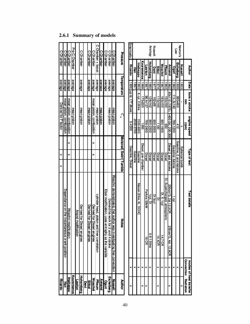
40
2.6.1 Summary of models
Au
tho
rD
ate
bo
re x
stro
ke
eng
ine s
peed
Typ
e o
f tes
tT
est d
eta
ils
mm
(rpm
)C
on
vectio
nR
ad
iatio
n
Nus
selt
192
3--
xS
pherica
l bom
bx
x
Eic
helb
erg
193
938
0x4
60
412
Gaso
line, 2
an
d 4
stroke
x
Og
uri
196
0114
.3x140
78
6-1
20
0G
aso
line 4
stroke
1 cy
lx
An
nan
d1
96
28
0x1
10
(1970
) 200-4
00 2
st, 2
00-3
00 4
st D
iese
l 2 a
nd
4stro
ke
200
cm^3
, 2st 1
2.3
CR
250
cm^3
, 4st 1
2.8
CR
xx
Pfla
um
196
315
0x1
90
650
Die
sel
DI, S
uperc
harg
ed, a
tmosp
heric
x
Wo
sc
hn
i1
96
716
5x1
55
60
0-1
60
0D
iese
lD
I, II, 1cyl
14.7
CR
x
Sitk
ei
197
411
0x1
40
1100
Die
sel
DI
14
.4C
Rx
x
Den
t1
97
7102
x05
60
0-2
00
0D
iese
lD
I 3cyl
Ho
hem
berg
198
012
8x1
42
60
0-2
30
0D
iese
l1cyl, D
I0.9
-1.9
litrex
Law
ton
198
798.4
x127
70
6-2
40
0D
iese
lP
erk
ins 5
0kW
16 C
Rx
x
Ko
ure
men
os
198
817
5x2
20
1000
Die
sel, p
re-ch
am
be
rx
x
Imab
ep
pu
199
36 c
yl, 2.0
litre15
00
-600
0G
aso
line
Nis
san
2litre
, 6L
DO
HC
x
Han
199
720
00
-370
0G
aso
line
x
Em
pirica
llyR
icard
o1
99
6u
p to
177
.8b
ore
0-4
500
Gaso
line, D
iesel
xx
New
ton's
Law
mo
des o
f heat tra
ns
fer
Nuss
elt
Ana
logy
Pre
ssu
reT
em
pe
ratu
reM
oto
red
Sw
irlT
um
ble
No
tes
Au
tho
r
C C
ham
be
ra
vera
ge
mea
n p
iston
Woschn
i de
mo
nstra
ted, th
at a
uth
or w
as in
ves
tigatin
g fre
e c
on
vectio
nN
uss
elt
C C
ham
be
ra
vera
ge
mea
n p
iston
De
rived h
is w
ork
for 2
an
d 4
stro
ke
Eic
he
lberg
C C
ham
be
ra
vera
ge
Els
er m
od
ificatio
n, u
ses e
ntro
ph
y a
s the
varia
ble
Og
uri
C C
ham
be
ra
vera
ge
mea
n p
iston
Ann
an
d
C C
ha
mbe
r + b
oo
st
ave
rag
em
ea
n p
iston
cylin
der h
ea
d, p
isto
n a
nd
liner c
orre
latio
nP
flau
mC
Ch
am
be
ra
vera
ge
me
an p
isto
n, c
om
bu
stio
nx
xD
erive
d fo
r Die
sel e
ngin
es
Wo
sc
hni
C C
ham
be
ra
vera
ge
mea
n p
iston
Derive
d fo
r Die
sel e
ngin
es
Sitk
ei
Den
t
C C
ham
be
ra
vera
ge
mea
n p
iston
Derive
d fo
r Die
sel e
ngin
es
Ho
he
mb
erg
Ana
nd
modifica
tion
Law
ton
Pre
-C.C
ha
mb
er
ave
rag
em
ea
n p
iston
Ko
ure
men
os
C C
ham
be
ra
vera
ge
me
an p
isto
n, c
om
bu
stio
nx
xW
osch
ni m
odific
atio
nIm
ab
ep
pu
C C
ham
be
ra
vera
ge
me
an p
isto
n, c
om
bu
stio
nD
epen
dan
ce o
n th
e in
sta
nta
ne
ou
s crank
po
sition
Ha
n
C C
ham
be
ra
vera
ge
Deriv
ed fo
r F fa
cto
rx
xR
icard
o
mC
Au
tho
rD
ate
bo
re x
stro
ke
eng
ine s
peed
Typ
e o
f tes
tT
est d
eta
ils
mm
(rpm
)C
on
vectio
nR
ad
iatio
n
Nus
selt
192
3--
xS
pherica
l bom
bx
x
Eic
helb
erg
193
938
0x4
60
412
Gaso
line, 2
an
d 4
stroke
x
Og
uri
196
0114
.3x140
78
6-1
20
0G
aso
line 4
stroke
1 cy
lx
An
nan
d1
96
28
0x1
10
(1970
) 200-4
00 2
st, 2
00-3
00 4
st D
iese
l 2 a
nd
4stro
ke
200
cm^3
, 2st 1
2.3
CR
250
cm^3
, 4st 1
2.8
CR
xx
Pfla
um
196
315
0x1
90
650
Die
sel
DI, S
uperc
harg
ed, a
tmosp
heric
x
Wo
sc
hn
i1
96
716
5x1
55
60
0-1
60
0D
iese
lD
I, II, 1cyl
14.7
CR
x
Sitk
ei
197
411
0x1
40
1100
Die
sel
DI
14
.4C
Rx
x
Den
t1
97
7102
x05
60
0-2
00
0D
iese
lD
I 3cyl
Ho
hem
berg
198
012
8x1
42
60
0-2
30
0D
iese
l1cyl, D
I0.9
-1.9
litrex
Law
ton
198
798.4
x127
70
6-2
40
0D
iese
lP
erk
ins 5
0kW
16 C
Rx
x
Ko
ure
men
os
198
817
5x2
20
1000
Die
sel, p
re-ch
am
be
rx
x
Imab
ep
pu
199
36 c
yl, 2.0
litre15
00
-600
0G
aso
line
Nis
san
2litre
, 6L
DO
HC
x
Han
199
720
00
-370
0G
aso
line
x
Em
pirica
llyR
icard
o1
99
6u
p to
177
.8b
ore
0-4
500
Gaso
line, D
iesel
xx
New
ton's
Law
mo
des o
f heat tra
ns
fer
Nuss
elt
Ana
logy
Pre
ssu
reT
em
pe
ratu
reM
oto
red
Sw
irlT
um
ble
No
tes
Au
tho
r
C C
ham
be
ra
vera
ge
mea
n p
iston
Woschn
i de
mo
nstra
ted, th
at a
uth
or w
as in
ves
tigatin
g fre
e c
on
vectio
nN
uss
elt
C C
ham
be
ra
vera
ge
mea
n p
iston
De
rived h
is w
ork
for 2
an
d 4
stro
ke
Eic
he
lberg
C C
ham
be
ra
vera
ge
Els
er m
od
ificatio
n, u
ses e
ntro
ph
y a
s the
varia
ble
Og
uri
C C
ham
be
ra
vera
ge
mea
n p
iston
Ann
an
d
C C
ha
mbe
r + b
oo
st
ave
rag
em
ea
n p
iston
cylin
der h
ea
d, p
isto
n a
nd
liner c
orre
latio
nP
flau
mC
Ch
am
be
ra
vera
ge
me
an p
isto
n, c
om
bu
stio
nx
xD
erive
d fo
r Die
sel e
ngin
es
Wo
sc
hni
C C
ham
be
ra
vera
ge
mea
n p
iston
Derive
d fo
r Die
sel e
ngin
es
Sitk
ei
Den
t
C C
ham
be
ra
vera
ge
mea
n p
iston
Derive
d fo
r Die
sel e
ngin
es
Ho
he
mb
erg
Ana
nd
modifica
tion
Law
ton
Pre
-C.C
ha
mb
er
ave
rag
em
ea
n p
iston
Ko
ure
men
os
C C
ham
be
ra
vera
ge
me
an p
isto
n, c
om
bu
stio
nx
xW
osch
ni m
odific
atio
nIm
ab
ep
pu
C C
ham
be
ra
vera
ge
me
an p
isto
n, c
om
bu
stio
nD
epen
dan
ce o
n th
e in
sta
nta
ne
ou
s crank
po
sition
Ha
n
C C
ham
be
ra
vera
ge
Deriv
ed fo
r F fa
cto
rx
xR
icard
o
mC
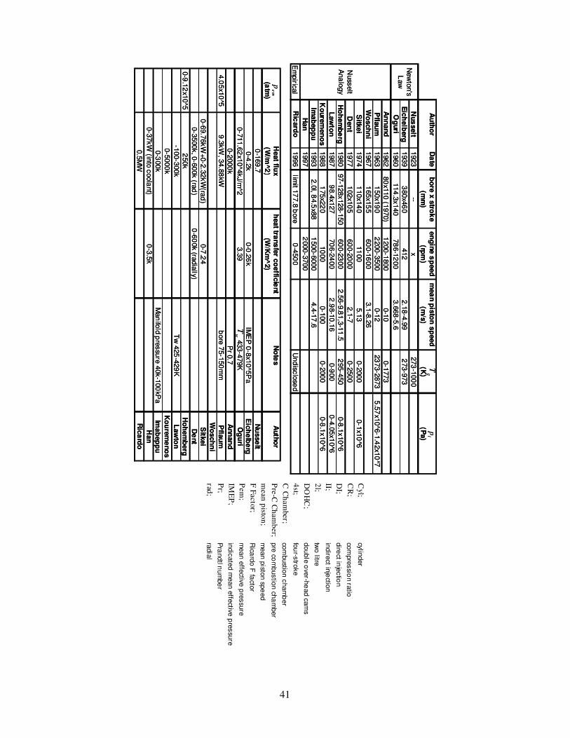
41
Cyl;
cylinder
CR
;co
mpre
ssio
n ra
tio
DI;
dire
ct inje
ctio
n
II;in
dire
ct inje
ction
2l;
two litre
DO
HC
;double
ove
r-he
ad ca
ms
4st;
fou
r-stro
ke
C C
ham
ber;
com
bustio
n c
ham
ber
Pre
-C C
ham
ber;
pre
com
bustio
n ch
am
ber
mean
pisto
n;
mean
pisto
n sp
eed
F F
acto
r;R
icard
o F
facto
r
Pem
;m
ean
effe
ctive p
ressu
re
IME
P;
indic
ate
d m
ean
effe
ctive p
ressu
re
Pr;
Pra
ndtl n
um
be
r
rad;
radia
l
Au
tho
rD
ate
bo
re x
stro
ke
en
gin
e s
peed
mea
n p
isto
n s
peed
(mm
)(rp
m)
(m/s
)(K
)(P
a)
Nus
selt
1923
--x
273
-100
0
Eic
helb
erg
1939
380x4
60
412
2.1
8-4
.99
273-9
73
Og
uri
1960
114
.3x140
78
6-1
200
3.6
68
-5.6
An
nand
1962
80
x110
(1970)
1200-1
800
0-1
00-1
773
Pfla
um
1963
150x1
90
2200-3
500
0-1
223
73-2
873
5.5
7x1
0^6
-1.4
2x1
07̂
Wo
sch
ni
1967
165x1
55
60
0-1
600
3.1
-8.2
6
Sitk
ei
1974
110x1
40
11
00
5.1
30-2
000
0-1
x10
6̂
Den
t1977
102x1
05
60
0-2
000
2.1
-70-2
500
Ho
hem
be
rg1980
97-1
28x128-1
50
60
0-2
300
2.5
6-9
.81,3
-11
.52
95-4
50
0-8
.1x10^6
Law
ton
1987
98.4
x127
70
6-2
400
2.9
8-1
0.1
60-9
00
0-4
.05x1
0^6
Ko
ure
men
os
1988
175x2
20
10
00
0-1
00
0-2
000
0-8
.1x10^6
Imab
ep
pu
1993
2.0
l, 84.5
x88
1500-6
000
4.4
-17
.6
Han
1997
2000-3
700
Em
pirica
lR
icard
o1996
limit 1
77.8
bore
0-4
50
0U
nd
isclo
sed
New
ton's
Law
Nuss
elt
Ana
logy
gT
ip
Heat flu
xh
eat tra
ns
fer c
oeffic
ient
No
tes
Auth
or
(atm
)(W
/m^2
)(W
/Km
^2)
0-1
69
.7N
usse
lt
0-4
.2k
0-0
.26
kIM
EP
0-8
x10^5
Pa
Eic
helb
erg
0-7
11.6
2x1
0^4
kJ/m
^23.3
9433-4
79K
Og
uri
0-2
000
kP
r 0.7
Ann
an
d
4.0
5x1
05̂
9.3
kW
, 34.8
8kW
bore
75-1
50
mm
Pfla
um
Wo
sch
ni
0-6
9.7
6kW
+0-2
.32kW
(rad
)0-7
.24
Sitk
ei
0-3
500k, 0
-600k (ra
d)
0-6
00k (ra
dia
lly)D
ent
0-9
.12
x10^5
250k
Ho
hem
berg
-100-3
00k
Tw
425
-429
KL
aw
ton
0-5
000
kK
ou
rem
eno
s
0-3
00k
Man
ifold
pre
ssu
re 4
0k-1
00
kPa
Imab
ep
pu
0-3
7kW
(into
coola
nt)
0-3
.5k
Han
0.5
MW
Ric
ard
o
em
p
wT
42
2.7 Description of thesis
An engine that is able to work in both two- and four-stroke configuration without the
need of changing any engine component, becomes a novelty because generates data
for both operation systems in the same configuration, while it provides accurate
results comparison between the two different firing modes. Unlike a conventional
two-stroke piston ported engine, the engine design is that of a poppet valve spark
ignition internal combustion engine. This is mainly devised to overcome the high
pollution restriction imposed by the law, while the four-stroke engine design
environment is well known.
This research project aims to improve the understanding of the heat transfer from the
combustion chamber to the surrounding metal and the coolant jacket, in both four-
and two-stroke configuration. This will generate literature about two-stroke operation
for such engine design. The engine test results come from the “2/4SIGHT” engine
project, this provides steady state thermal data and instantaneous engine performance
results, that can be compared to the energy balance calculation, the heat flux and heat
transfer coefficient. Of particular interest is the maximum torque data where the heat
transfer generates its peak values.
Chapter 2 Literature review where a resume an introduction to the internal
combustion engine is provided, together with the energy balance generation and
calculation. This includes an introduction and a resume of the literature, through a
comparison of the different correlations given. A more comprehensive resume is also
available in Appendix A, where the different authors work a explained
chronologically.
Chapter 3; Experimental studies where the characteristics of the experimental facility
are explained together with the main hardware provided for this study. The devised
thermal survey defines the engine cooling strategy providing the best working
conditions. The way the thermal data is collected, together with the relevant steady
state and instantaneous data, the way the thermal analysis work is also explained.
While also the data sets to be correlated are provided.

43
Results of the engine tests, the heat flux results, the heat transfer coefficient and their
comparison together with those of the energy balance in each case are reported in
Chapter 4; Experimental results.
The thesis is summarised and the conclusions of the experimental analysis are
summarised in Chapter 5; Conclusions.
Recommendation for any future work is given in Chapter 6 Recommendations for
further work.
44
3 Experimental studies
3.1 Introduction
Experimental studies have come a long way since their inception. Nowadays, the
accuracy is extremely high. A wide variety of parameters can be studied using
purpose built instrumentation. The experiments are used to determine engine
performance, reliability and emissions. In addition, the experimental instrumentation
can be used to quantify the heat transfer within the engine, in what is called a thermal
study. This is achieved by inserting thermocouples into the metal and coolant, close to
the combustion chamber.
In this study, two, steady-state operating conditions were investigated: peak engine
torque and peak engine power. The thermal data obtained from the engine were
compared with the different mathematical models considered previously in Chapter 2.
The experiments were performed in both four-stroke and two-stroke operation using
the same engine set-up. The data were also compared to the empirical Ricardo heat
flux correlation for steady-state conditions. The instantaneous local gas temperature
could not be measured. Instead a mean gas temperature close to the wall was inferred
from extrapolation of the heat flux from measurements obtained in the metal.
3.2 Experimental research engine facility
The 2/4SIGHT engine is installed in a test-cell at the Sir Harry Ricardo Laboratories
in the University of Brighton. The installation is shown in Figure 9. The test cell
comprises a control room and separate engine test bed. The engine is a highly
advanced research tool equipped with a fully flexible hydraulic valve-train. This
enables the engine to uniquely switch between two-stroke and four-stroke operation.
It is a poppet valve engine design layout, that avoids the two-stroke, piston ported,
engine drawbacks, while allowing optimal performance for four-stroke operation.
Two-stroke operation is activated where high torque is required. This results in
significant improvements in fuel economy due to the potential for downsizing of the
engine capacity. A more detailed description is given in (Osborne et al., (2008)).

45
Figure 9: Test cell and control room overall view.
An overview of the instrumentation used in this study is shown in Figure 10.
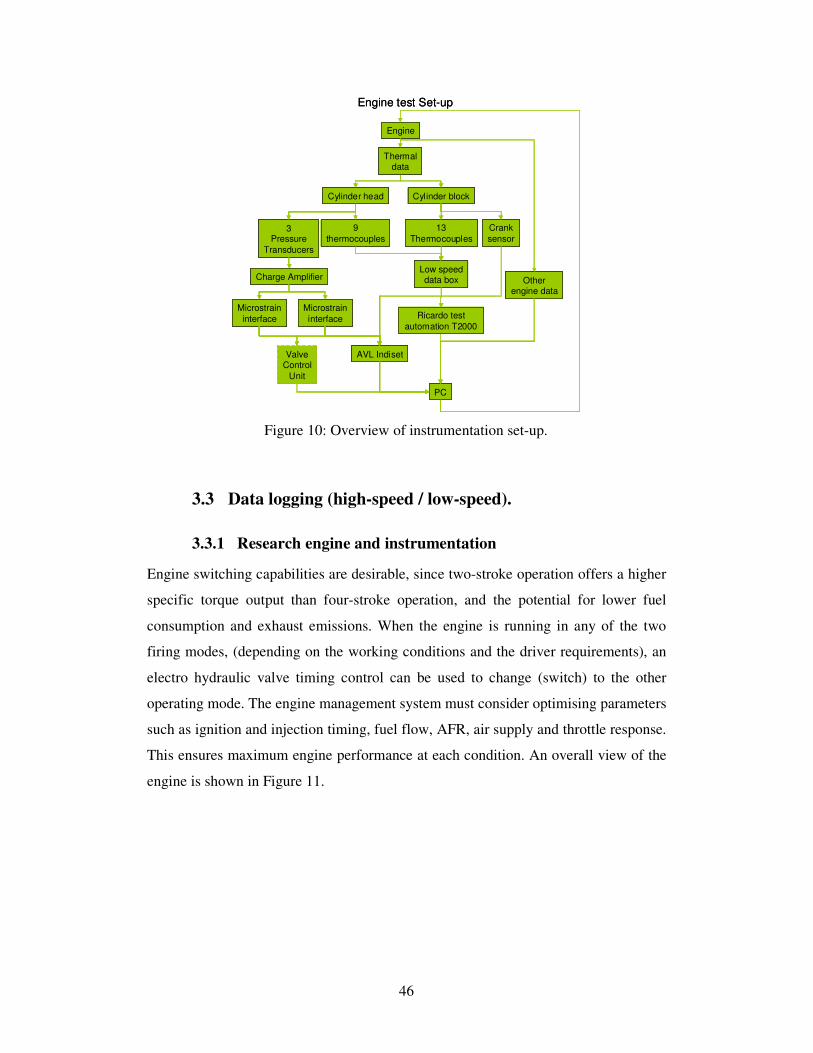
46
Figure 10: Overview of instrumentation set-up.
3.3 Data logging (high-speed / low-speed).
3.3.1 Research engine and instrumentation
Engine switching capabilities are desirable, since two-stroke operation offers a higher
specific torque output than four-stroke operation, and the potential for lower fuel
consumption and exhaust emissions. When the engine is running in any of the two
firing modes, (depending on the working conditions and the driver requirements), an
electro hydraulic valve timing control can be used to change (switch) to the other
operating mode. The engine management system must consider optimising parameters
such as ignition and injection timing, fuel flow, AFR, air supply and throttle response.
This ensures maximum engine performance at each condition. An overall view of the
engine is shown in Figure 11.
Engine
Cylinder head Cylinder block
13
Thermocouples3
Pressure
Transducers
Low speeddata box
9
thermocouples
AVL Indiset
Crank
sensor
Otherengine data
PC
Microstrain
interface
Microstrain
interface
Engine test Set-up
Charge Amplifier
ValveControl
Unit
Ricardo test
automation T2000
Thermaldata
Engine
Cylinder head Cylinder block
13
Thermocouples3
Pressure
Transducers
Low speeddata box
9
thermocouples
AVL Indiset
Crank
sensor
Otherengine data
PC
Microstrain
interface
Microstrain
interface
Engine test Set-up
Charge Amplifier
ValveControl
Unit
Ricardo test
automation T2000
Thermaldata
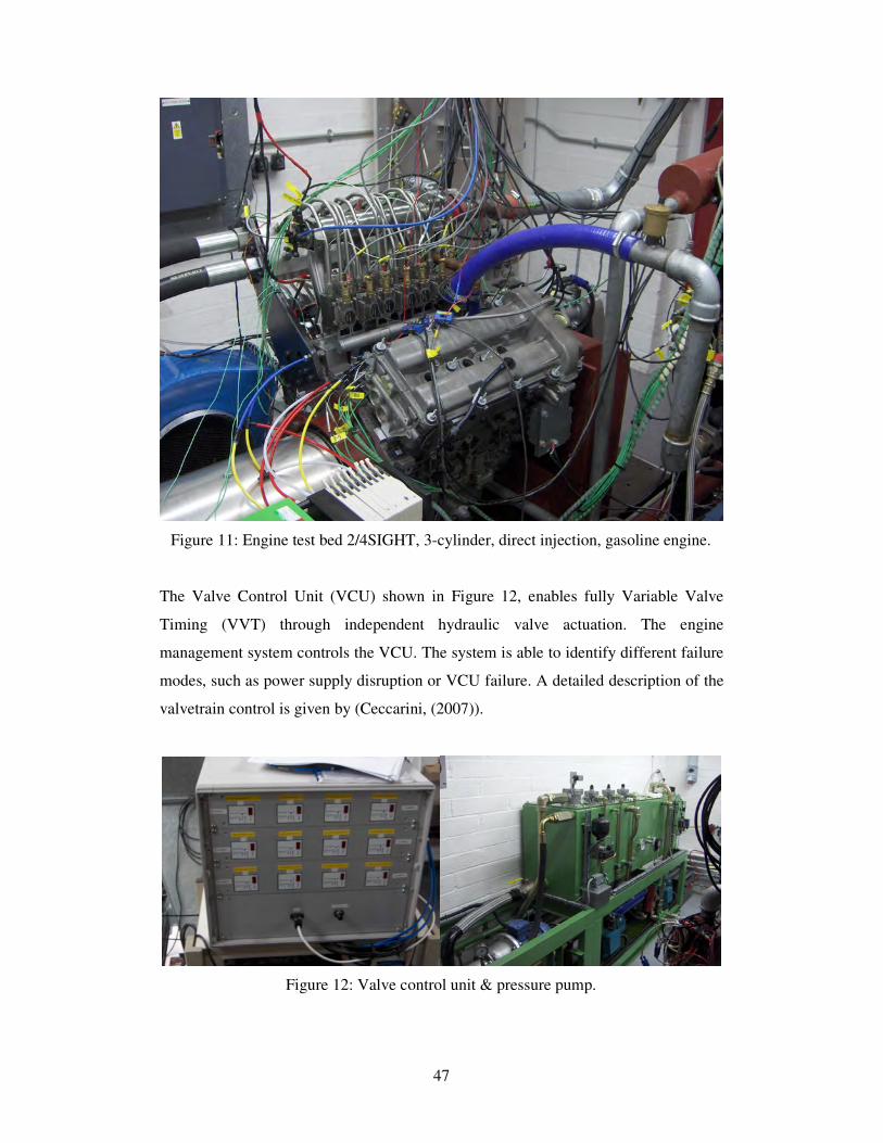
47
Figure 11: Engine test bed 2/4SIGHT, 3-cylinder, direct injection, gasoline engine.
The Valve Control Unit (VCU) shown in Figure 12, enables fully Variable Valve
Timing (VVT) through independent hydraulic valve actuation. The engine
management system controls the VCU. The system is able to identify different failure
modes, such as power supply disruption or VCU failure. A detailed description of the
valvetrain control is given by (Ceccarini, (2007)).
Figure 12: Valve control unit & pressure pump.
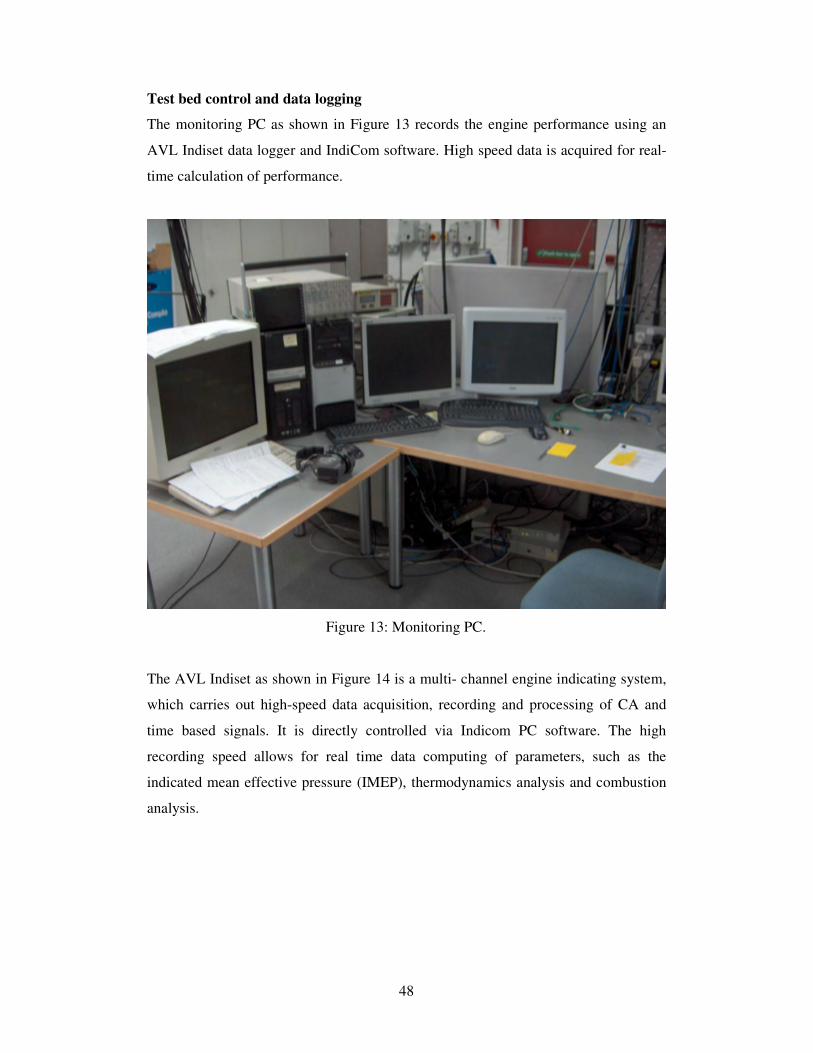
48
Test bed control and data logging
The monitoring PC as shown in Figure 13 records the engine performance using an
AVL Indiset data logger and IndiCom software. High speed data is acquired for real-
time calculation of performance.
Figure 13: Monitoring PC.
The AVL Indiset as shown in Figure 14 is a multi- channel engine indicating system,
which carries out high-speed data acquisition, recording and processing of CA and
time based signals. It is directly controlled via Indicom PC software. The high
recording speed allows for real time data computing of parameters, such as the
indicated mean effective pressure (IMEP), thermodynamics analysis and combustion
analysis.

49
Figure 14: AVL Indiset front and rear view.
The T2000 Ricardo-Schenk-Horiba Test-bed controller system
The test-bed Automation system is shown in Figure 15. The system controls the test-
bed, functionality, operating conditions, data collection, engine settings, data
acquisition, running conditions, calculations and parameterisation as well as low
speed data acquisition.
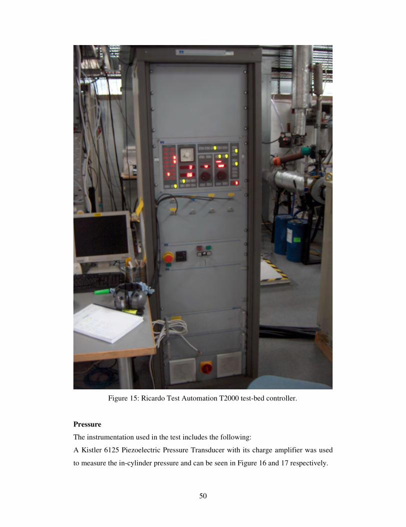
50
Figure 15: Ricardo Test Automation T2000 test-bed controller.
Pressure
The instrumentation used in the test includes the following:
A Kistler 6125 Piezoelectric Pressure Transducer with its charge amplifier was used
to measure the in-cylinder pressure and can be seen in Figure 16 and 17 respectively.

51
Figure 16: Piezoelectric pressure transducer.

52
Figure 17: Charge amplifier.
Intake and exhaust pressure were measured using a 4045A2 Kistler absolute pressure
transducer.
Valve Timing Location and Lift
A Microstrain Interface and a LVDT (Linear Variable Differential Transducer)
displacement transducer as shown in Figure 18, was used to communicate the actual
valve position and lift between the VCU and the EMS (Engine Management System).
The valve lift was also recorded by the AVL Indiset.
Figure 18: Microstrain interface.
Fuel
The Max meter shown in Figure 19 measured the volume flow rate of fuel.
53
Figure 19: Max flow meter (courtesy of Maxmachinery)
3.4 Thermal Survey
Engine cooling is required to maintain correct engine temperature. A cooling strategy
was devised by Ricardo, to overcome the extra heat produced while running in two-
stroke operation. The critical area is in the bridge between the pair of exhaust valves.
3.4.1 Cooling Strategy
The cooling strategy defined how the coolant flowed through the coolant jacket
passages. An efficient strategy maximises the principle of heat transfer from metal to
coolant, preventing overheating, ideally maintaining a gross running temperature
close to 80oC, during most of the engine running conditions. This may be obtained by
devising a coolant jacket that ensures that the coolant flows to the required areas only;
using the minimum volume possible and eliminating dead ends; increasing flow
velocity and reducing coolant pressure where required. Figure 20 shows the engine
coolant core (coolant only). The top part shows a ramp shape to improve the
degassing and reduce possible boiling effects at critical areas. Inlet and exhaust valve
bridge cooling are also shown, together with an extra coolant passage from the engine
block to the cylinder head, through each exhaust valve bridge.
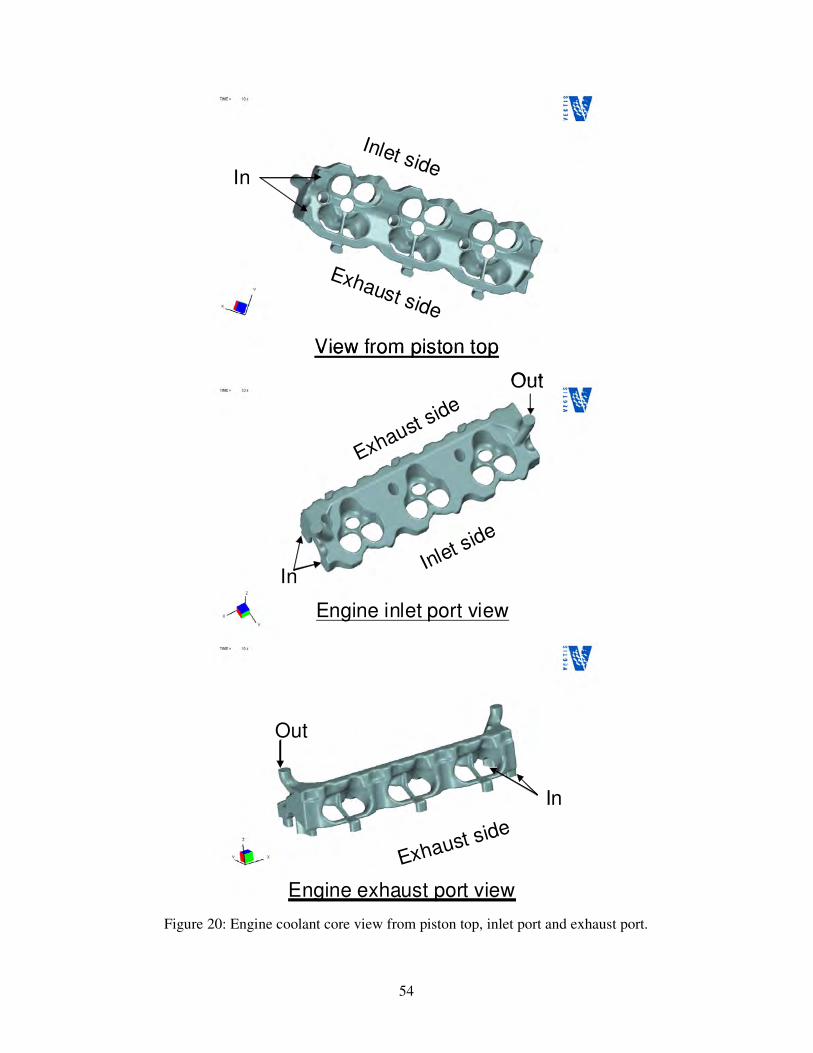
54
Figure 20: Engine coolant core view from piston top, inlet port and exhaust port.
Exhaust side
Engine exhaust port view
Out
In
Exhaust side
Engine exhaust port view
Out
In
Inlet side
Exhaust side
Engine inlet port view
In
Out
Inlet side
Exhaust side
Engine inlet port view
In
Out
Inlet side
Exhaust side
View from piston top
In
Inlet side
Exhaust side
View from piston top
In
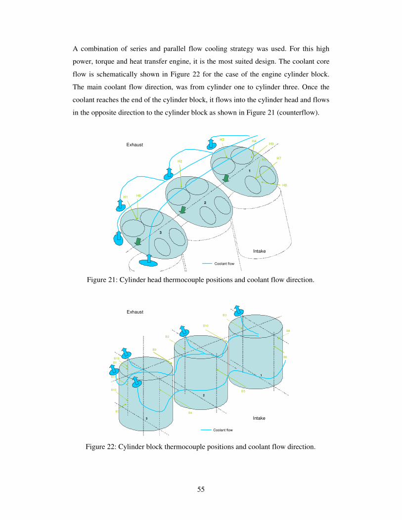
55
A combination of series and parallel flow cooling strategy was used. For this high
power, torque and heat transfer engine, it is the most suited design. The coolant core
flow is schematically shown in Figure 22 for the case of the engine cylinder block.
The main coolant flow direction, was from cylinder one to cylinder three. Once the
coolant reaches the end of the cylinder block, it flows into the cylinder head and flows
in the opposite direction to the cylinder block as shown in Figure 21 (counterflow).
Figure 21: Cylinder head thermocouple positions and coolant flow direction.
Figure 22: Cylinder block thermocouple positions and coolant flow direction.
1
2
3
H1
H2
H3 H4
H7
H8
H9
H6
H5
Intake
Exhaust
Coolant flow
1
2
3
H1
H2
H3 H4
H7
H8
H9
H6
H5
Intake
Exhaust
Coolant flow
1
2
3
B1
B2
B3
B4
B5
B6
B7
B8
B9
B10
B11
B12
B13
Intake
Exhaust
Coolant flow
1
2
3
B1
B2
B3
B4
B5
B6
B7
B8
B9
B10
B11
B12
B13
Intake
Exhaust
Coolant flow
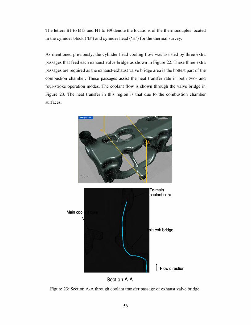
56
The letters B1 to B13 and H1 to H9 denote the locations of the thermocouples located
in the cylinder block (‘B’) and cylinder head (‘H’) for the thermal survey.
As mentioned previously, the cylinder head cooling flow was assisted by three extra
passages that feed each exhaust valve bridge as shown in Figure 22. These three extra
passages are required as the exhaust-exhaust valve bridge area is the hottest part of the
combustion chamber. These passages assist the heat transfer rate in both two- and
four-stroke operation modes. The coolant flow is shown through the valve bridge in
Figure 23. The heat transfer in this region is that due to the combustion chamber
surfaces.
Figure 23: Section A-A through coolant transfer passage of exhaust valve bridge.
Section A-A
Main coolant core
Exh-exh bridge
Flow direction
To maincoolant core
Section A-A
Main coolant core
Exh-exh bridge
Flow direction
To maincoolant core
A
A
A
A

57
Coolant Flow Rate
The engine coolant flow rate was measured over a range of coolant temperatures. The
coolant was pumped externally using a Wilo TOP-S30/10 water pump. The maximum
estimated error of ±0.64 l/min was due to the uncertainty of ±1% in the turbine flow-
meter. The test results can be seen in Table 6.
FLOW MEASUREMENTS
Engine Temp out (degC) Flow Meter out (Hz) Flow (l/min)
18 434 62.96697
25 434 62.96697
40 436 63.25579
50 434 62.96697
70 438 63.54463
80 438 63.54463
85 438 63.54463
Table 6: Results of coolant flow rate measurements.
3.4.2 Coolant Fluid Properties
Boiling can become a very dangerous effect since it may cause overheating, which
may develop into poor combustion, thermal fatigue and possible component failure.
Therefore the choice of coolant is important. Typically the coolant fluid is mainly
water, due to its high enthalpy of vaporization, high thermal conductivity, high
saturation temperature and high specific heat. It is considered a highly effective
cooling medium, although its freezing point and corrosion nature are less convenient
properties for this work. To improve these negative properties, the water is mixed
with ethylene glycol. Table 7 shows the typical engine coolant properties with
temperature, which has additional dissolved additives such as metal corrosion
inhibitors, antifoam additive, a dye to simplify identification and alkaline substances
to neutralize acids. All the components are mixed with a defined amount of water.
The coolant fluid removes heat from the engine by the following processes: forced
convection, sub-cooled boiling, nucleate boiling and saturated boiling. Forced
convection was defined in the previous chapter. Here sub-cooled boiling is defined as
“bubble detachment when it is small and collapses into the bulk fluid that is below its
saturation temperature” (Milton, (1995)). Nucleate boiling takes place when bubbles
grow in separate areas whilst some coolant remains in contact with the surface.
58
Saturated boiling appears when film boiling occurs and a “vapour blanket” appear at
the metal surface and “large bubbles and no condensation take place in the bulk
fluid” (Milton, (1995)). During boiling heat transfer, the metal temperature increases,
through the combination of nucleate boiling and convection. The heat addition is
given by Eq.3.4-1.
( ) ( )swblwc TThTThq −+−= 3.4-1
where Tl is the bulk liquid temperature, Ts is the fluid saturation temperature, hc is the
heat transfer coefficient for turbulent forced convection and hb is the heat transfer
coefficient for boiling conditions. hc may be obtained through the Dittus-Boelter
correlation in Eq.3.4-2 and hb through Chen correlation (1966) (Milton, (1995))
(Eq.3.4-3).
4.08.0PrRe023.0=Nu 3.4-2
where H
cD
kNuh =
where DH is the diameter of the pipe hole.
( ) SpTTh
ckh ssw
vfg
p
b
75.024.0
24.029.029.05.0
49.045.079.0
00122.0 ∆−
=
ρµσ
ρ 3.4-3
ppp sats −=∆
where σt is the surface tension, hig is the enthalpy of vaporisation, ∆ps is the saturated
pressure, S is the suppression factor, psat is the saturated pressure at wall temperature
condition and p is the fluid pressure.
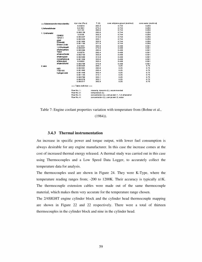
59
Table 7: Engine coolant properties variation with temperature from (Bohne et al.,
(1984)).
3.4.3 Thermal instrumentation
An increase in specific power and torque output, with lower fuel consumption is
always desirable for any engine manufacturer. In this case the increase comes at the
cost of increased thermal energy released. A thermal study was carried out in this case
using Thermocouples and a Low Speed Data Logger, to accurately collect the
temperature data for analysis.
The thermocouples used are shown in Figure 24. They were K-Type, where the
temperature reading ranges from; -200 to 1200K. Their accuracy is typically ±1K.
The thermocouple extension cables were made out of the same thermocouple
material, which makes them very accurate for the temperature range chosen.
The 2/4SIGHT engine cylinder block and the cylinder head thermocouple mapping
are shown in Figure 22 and 22 respectively. There were a total of thirteen
thermocouples in the cylinder block and nine in the cylinder head.
d yn visc (Pa.s) T (K) c onc et hy len e g lycol (m ol/mo l) conc water (m ol/m ol)
0 .0 324 3 26 3 .3 0 .7 44 0.25 6
0 .0 189 1 27 3 .4 0 .7 44 0.25 60 .0 1 23 28 2 .6 0 .7 44 0.25 6
0. 00 8 139 29 2 .6 0 .7 44 0.25 6
0 .0 0 58 30 2 .3 0 .7 44 0.25 6
0. 00 4 207 31 2 .6 0 .7 44 0.25 6
0. 00 2 433 33 3 .1 0 .7 44 0.25 6
0. 00 1 664 35 2 .9 0 .7 44 0.25 60. 00 1 193 37 1 .9 0 .7 44 0.25 6
0 .0 122 2 26 3 .9 0 .4 99 0.50 10. 00 8 057 27 2 .8 0 .4 99 0.50 1
0. 00 5 366 28 2 .6 0 .4 99 0.50 1
0 .0 037 8 29 2 .4 0 .4 99 0.50 1
0. 00 2 732 30 2 .8 0 .4 99 0.50 1
0. 00 2 069 31 2 .8 0 .4 99 0.50 1
0. 00 1 309 33 3 .6 0 .4 99 0.50 1
0 .0 009 2 35 3 .4 0 .4 99 0.50 1
0. 00 0 799 37 3 .8 0 .4 99 0.50 10. 00 5 024 26 6 .1 0. 25 0 .7 5
0. 00 2 591 28 2 .6 0. 25 0 .7 5
0. 00 1 892 29 2 .4 0. 25 0 .7 5
0. 00 1 448 30 2 .4 0. 25 0 .7 5
0. 00 1 125 31 3 .1 0. 25 0 .7 5
0. 00 0 769 33 3 .1 0. 25 0 .7 5
0. 00 0 578 35 3 .1 0. 25 0 .7 5
0. 00 0 517 36 2 .9 0. 25 0 .7 5
+++ Tab le d e fin ition +++
Row N o. 1 : viscos ity, d yn am ic (L ) , rec om m en ded
Row N o. 2 : temp erat ure (L)
Row N o. 3 : conc entra tio n (L) , com po nen t 1 , 1 ,2 -et haned io l
Row N o. 4 : conc entra tio n (L) , com po nen t 2 , water
+++ Substance and/or mixture identificat ion +++
1,2-ethanediol/water
1. 1,2-ethanediol
C2H6O2
107-21-1
glycolEthanediol
Ethane-1,2-diol
1,2-Dihydroxyethane
dihydroxyethaneTescol
ethylene dihydrate
ethylene glycol
monoethylene glycolethlene glycol
ethylene alcohol
2. water
H2O7732-18-5
hydrogen oxide

60
Figure 24: Type K thermocouple.
The Data Logger is shown in Figure 25. It continuously recorded the thermocouple
data, where a standard data format was utilised. The sample rate was limited to a few
Hertz. For long periods of time a large memory size was required.
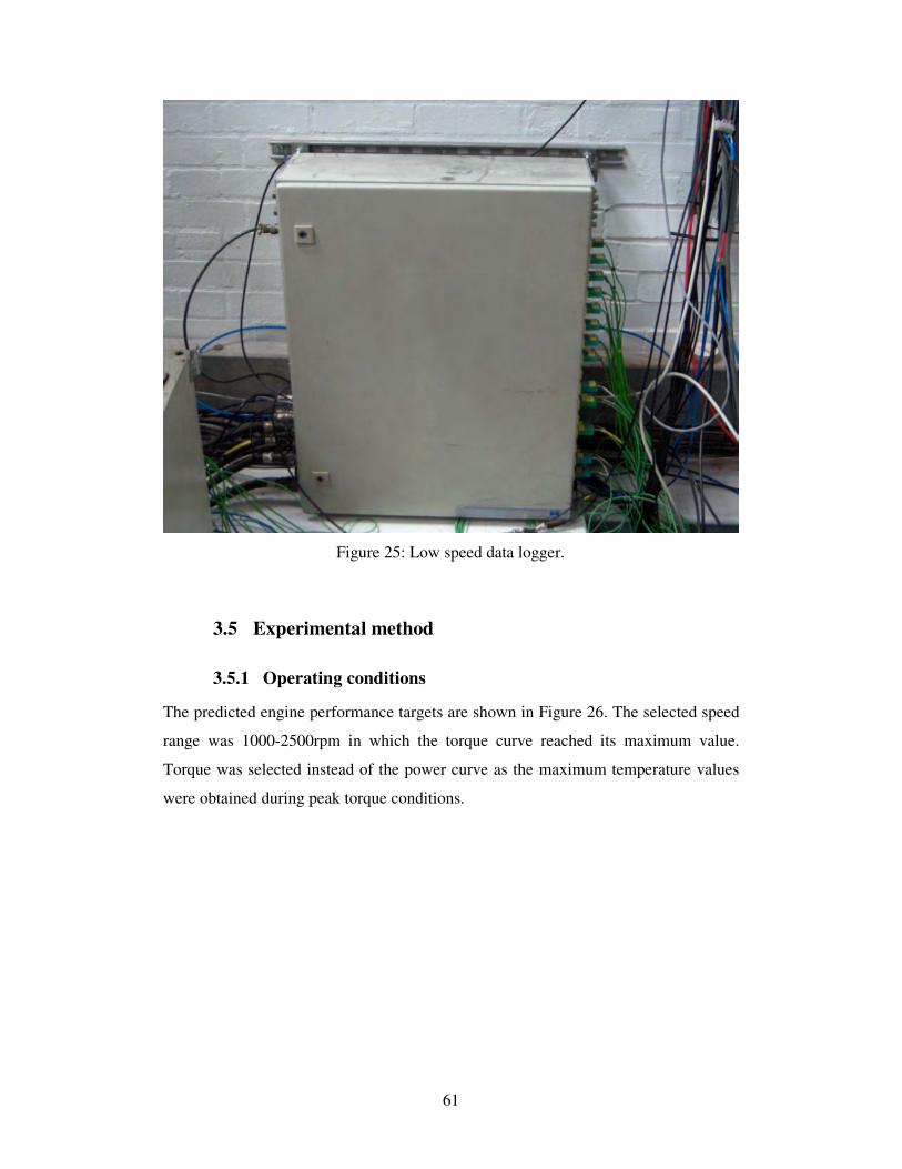
61
Figure 25: Low speed data logger.
3.5 Experimental method
3.5.1 Operating conditions
The predicted engine performance targets are shown in Figure 26. The selected speed
range was 1000-2500rpm in which the torque curve reached its maximum value.
Torque was selected instead of the power curve as the maximum temperature values
were obtained during peak torque conditions.
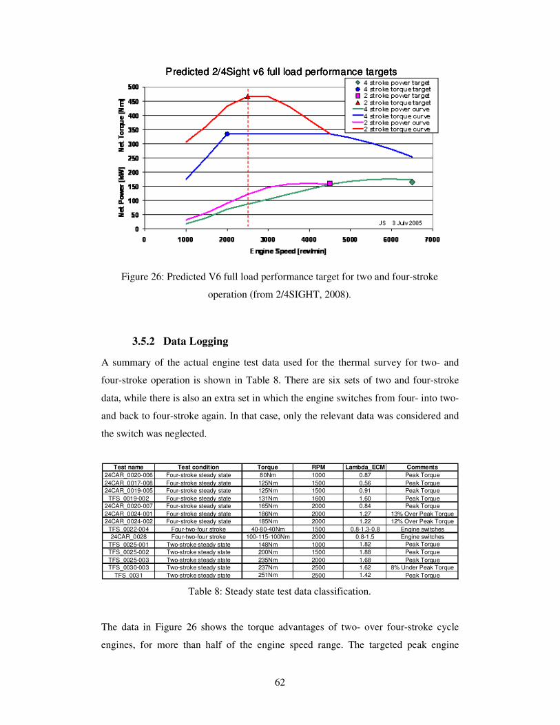
62
Figure 26: Predicted V6 full load performance target for two and four-stroke
operation (from 2/4SIGHT, 2008).
3.5.2 Data Logging
A summary of the actual engine test data used for the thermal survey for two- and
four-stroke operation is shown in Table 8. There are six sets of two and four-stroke
data, while there is also an extra set in which the engine switches from four- into two-
and back to four-stroke again. In that case, only the relevant data was considered and
the switch was neglected.
Table 8: Steady state test data classification.
The data in Figure 26 shows the torque advantages of two- over four-stroke cycle
engines, for more than half of the engine speed range. The targeted peak engine
Predicted 2/4Sight v6 full load performance targetsPredicted 2/4Sight v6 full load performance targetsPredicted 2/4Sight v6 full load performance targets
Test name Test condition Torque RPM Lambda_ECM Comments
24CAR_0020-006 Four-stroke steady state 80Nm 1000 0.87 Peak Torque
24CAR_0017-008 Four-stroke steady state 125Nm 1500 0.56 Peak Torque
24CAR_0019-005 Four-stroke steady state 125Nm 1500 0.91 Peak Torque
TFS_0019-002 Four-stroke steady state 131Nm 1600 1.60 Peak Torque
24CAR_0020-007 Four-stroke steady state 165Nm 2000 0.84 Peak Torque
24CAR_0024-001 Four-stroke steady state 186Nm 2000 1.27 13% Over Peak Torque
24CAR_0024-002 Four-stroke steady state 185Nm 2000 1.22 12% Over Peak Torque
TFS_0022-004 Four-two-four stroke 40-80-40Nm 1500 0.8-1.3-0.8 Engine switches
24CAR_0028 Four-two-four stroke 100-115-100Nm 2000 0.8-1.5 Engine switches
TFS_0025-001 Two-stroke steady state 148Nm 1000 1.82 Peak Torque
TFS_0025-002 Two-stroke steady state 200Nm 1500 1.88 Peak Torque
TFS_0025-003 Two-stroke steady state 235Nm 2000 1.68 Peak Torque
TFS_0030-003 Two-stroke steady state 237Nm 2500 1.62 8% Under Peak Torque
TFS_0031 Two-stroke steady state 251Nm 2500 1.42 Peak Torque
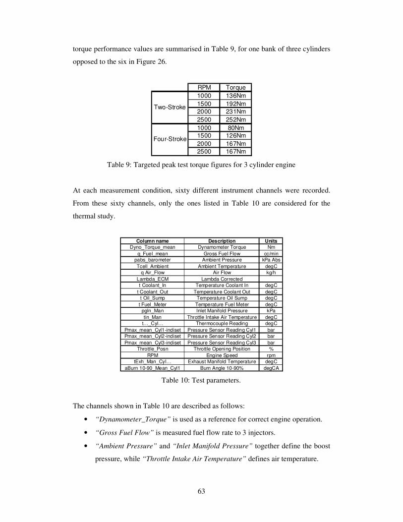
63
torque performance values are summarised in Table 9, for one bank of three cylinders
opposed to the six in Figure 26.
Table 9: Targeted peak test torque figures for 3 cylinder engine
At each measurement condition, sixty different instrument channels were recorded.
From these sixty channels, only the ones listed in Table 10 are considered for the
thermal study.
Table 10: Test parameters.
The channels shown in Table 10 are described as follows:
• “Dynamometer_Torque” is used as a reference for correct engine operation.
• “Gross Fuel Flow” is measured fuel flow rate to 3 injectors.
• “Ambient Pressure” and “Inlet Manifold Pressure” together define the boost
pressure, while “Throttle Intake Air Temperature” defines air temperature.
Column name Description Units
Dyno_Torque_mean Dynamometer Torque Nm
q_Fuel_mean Gross Fuel Flow cc/min
pabs_barometer Ambient Pressure kPa Abs
Tcell_Ambient Ambient Temperature degC
q Air_Flow Air Flow kg/h
Lambda_ECM Lambda Corrected
t Coolant_In Temperature Coolant In degC
t Coolant_Out Temperature Coolant Out degC
t Oil_Sump Temperature Oil Sump degC
t Fuel_Meter Temperature Fuel Meter degC
pgln_Man Inlet Manifold Pressure kPa
tin_Man Throttle Intake Air Temperature degC
t…_Cyl… Thermocouple Reading degC
Pmax_mean_Cyl1-indiset Pressure Sensor Reading Cyl1 bar
Pmax_mean_Cyl2-indiset Pressure Sensor Reading Cyl2 bar
Pmax_mean_Cyl3-indiset Pressure Sensor Reading Cyl3 bar
Throttle_Posn Throttle Opening Position %
RPM Engine Speed rpm
tExh_Man_Cyl… Exhaust Manifold Temperature degC
aBurn 10-90_Mean_Cyl1 Burn Angle 10-90% degCA
RPM Torque
1000 136Nm
1500 192Nm
2000 231Nm
2500 252Nm
1000 80Nm
1500 126Nm
2000 167Nm
2500 167Nm
Two-Stroke
Four-Stroke
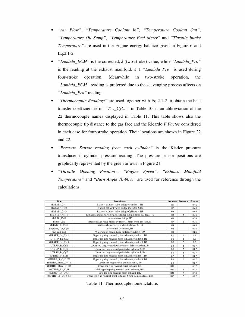
64
• “Air Flow”, “Temperature Coolant In”, “Temperature Coolant Out”,
“Temperature Oil Sump”, “Temperature Fuel Meter” and “Throttle Intake
Temperature” are used in the Engine energy balance given in Figure 6 and
Eq.2.1-2.
• “Lambda_ECM” is the corrected, λ (two-stroke) value, while “Lambda_Pro”
is the reading at the exhaust manifold. λ=1 “Lambda_Pro” is used during
four-stroke operation. Meanwhile in two-stroke operation, the
“Lambda_ECM” reading is preferred due to the scavenging process affects on
“Lambda_Pro” reading.
• “Thermocouple Readings” are used together with Eq.2.1-2 to obtain the heat
transfer coefficient term. “T…_Cyl…” in Table 10, is an abbreviation of the
22 thermocouple names displayed in Table 11. This table shows also the
thermocouple tip distance to the gas face and the Ricardo F Factor considered
in each case for four-stroke operation. Their locations are shown in Figure 22
and 22.
• “Pressure Sensor reading from each cylinder” is the Kistler pressure
transducer in-cylinder pressure reading. The pressure sensor positions are
graphically represented by the green arrows in Figure 21.
• “Throttle Opening Position”, “Engine Speed”, “Exhaust Manifold
Temperature” and “Burn Angle 10-90%” are used for reference through the
calculations.
Table 11: Thermocouple nomenclature.
Title Description Location Distance F factor
tExExBr_Cyl1 Exhaust-exhaust valve bridge cylinder 1, H1 H1 0.45
tExExBr_Cyl2 Exhaust-exhaust valve bridge Cylinder 2, H2 H2 0.45
tExExBr_Cyl3 Exhaust-exhaust valve bridge Cylinder3, H3 H3 0.45
tExExBr_Cyl1_6 Exhaust-exhaust valve bridge cylinder 1, 8mm from gas face, H6 H6 8 0.45
tInInBr_Cyl1 Intake-intake bridge H5 H5 0.75
tInInBr_Cyl3 Intake-intake valve bridge cylinder 1, 8mm from gas face, H7 H7 8 0.75
tInExBr_R_Cyl1 Intake-exhaust valve bridge, Cylinder 1, H4 H4 0.65
tInjector_Tip_Cyl1 injector tip Cylinder1, H8 H8 0.35
tCylHead_Bulk Water out of block (head outlet) cylinder 3, H9 H9 0.25
tUTRRP_Ex_Cyl1 Opper top ring reversal point exhaust cylinder 1, B1 B1 5 0.3
tUTRRP_Ex_Cy2 Upper top ring reversal point exhaust cylinder 2, B2 B2 5 0.3
tUTRRP_Ex_Cyl3 Upper top ring reversal point exhaust cylinder 3, B3 B3 5 0.3
tUTRRP_In_Cyl1 Upper top ring reversal point exhaust inlet cylinder1, B4 B4 5 0.27
tUTRRP_In_Cyl2 Upper top ring reversal point inlet cylinder 2, B5 B5 5 0.27
tUTRRP_In_Cyl3 Upper top ring reversal point inlet cylinder 3, B6 B6 5 0.27
tUTRRP_F_Cyl1 Upper top ring reversal point exhaust cylinder 1, B7 B7 5 0.27
tUTRRP_R_Cyl3??? Upper top ring reversal point exhaust cylinder 3, B8 B8 5 0.27
tUTRRP_IBore_Cyl12 Upper top ring reversal point exhaust, B9 B9 0.27
tUTRRP_IBore_Cyl23 Upper top ring reversal point exhaust, B10 B10 0.17
tMTRRP_Ex_Cyl3 Mid-upper top ring reversal point exhaust, B11 B11 5 0.17
tLTRRP_Ex_Cyl3 Low-top ring reversal point exhaust, B12 B12 5 0.16
tUTTRP_Ex_Cyl3_13 Upper top ring reversal point exhaust, 5 mm from gas face, B13 B13 5 0.27
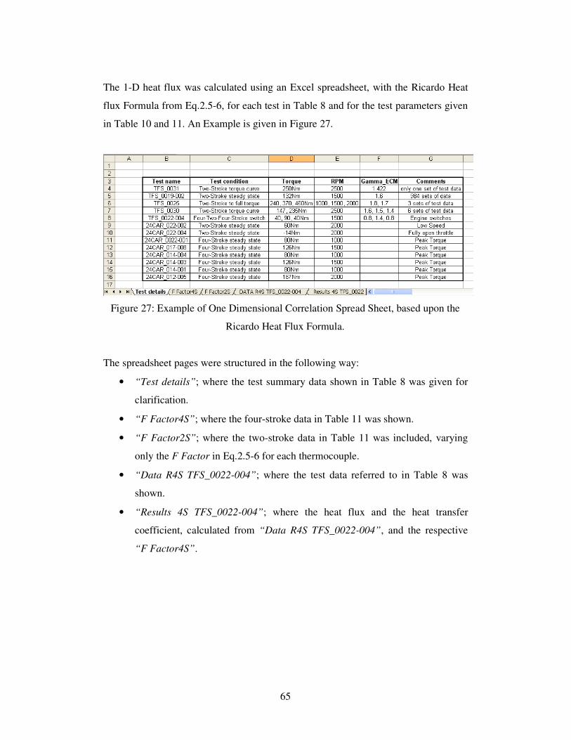
65
The 1-D heat flux was calculated using an Excel spreadsheet, with the Ricardo Heat
flux Formula from Eq.2.5-6, for each test in Table 8 and for the test parameters given
in Table 10 and 11. An Example is given in Figure 27.
Figure 27: Example of One Dimensional Correlation Spread Sheet, based upon the
Ricardo Heat Flux Formula.
The spreadsheet pages were structured in the following way:
• “Test details”; where the test summary data shown in Table 8 was given for
clarification.
• “F Factor4S”; where the four-stroke data in Table 11 was shown.
• “F Factor2S”; where the two-stroke data in Table 11 was included, varying
only the F Factor in Eq.2.5-6 for each thermocouple.
• “Data R4S TFS_0022-004”; where the test data referred to in Table 8 was
shown.
• “Results 4S TFS_0022-004”; where the heat flux and the heat transfer
coefficient, calculated from “Data R4S TFS_0022-004”, and the respective
“F Factor4S”.

66
4 Experimental results
4.1 Summary of engine performance
The combined two- and four-stroke engine operating strategy is shown in Figure 28
for the three cylinder engine given in Table 9. The plot shows that two-stroke over
four-stroke operation is better suited for high load working conditions, offering an
increase in net torque over approximately a third of the engine speed range. This
drops after 3000 rpm, up to 4500 rpm, where it generates equal torque levels to four-
stroke operation. Where there is no need for high engine torque, four-stroke
configuration is preferred for reduced emissions and lower fuel consumption
(Osborne et al., (2008)).
Figure 28: Engine overall operating strategy from (Ricardo, (2008)).
The topology of the 2/4SIGHT engine is shown in Figure 29. The main characteristic
of this engine is the separate supercharger and turbocharger drive configurations. This
is because the scavenging needs of two-stroke operation requires a supercharger to
deliver the necessary boost, since at high speeds, two-stroke poppet valve engines
may produce knock. Meanwhile in four-stroke operation, a waste-gate turbocharger
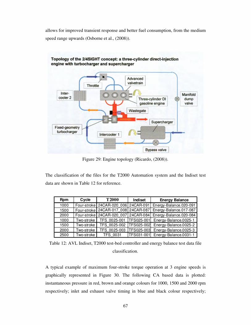
67
allows for improved transient response and better fuel consumption, from the medium
speed range upwards (Osborne et al., (2008)).
Figure 29: Engine topology (Ricardo, (2008)).
The classification of the files for the T2000 Automation system and the Indiset test
data are shown in Table 12 for reference.
Table 12: AVL Indiset, T2000 test-bed controller and energy balance test data file
classification.
A typical example of maximum four-stroke torque operation at 3 engine speeds is
graphically represented in Figure 30. The following CA based data is plotted:
instantaneous pressure in red, brown and orange colours for 1000, 1500 and 2000 rpm
respectively; inlet and exhaust valve timing in blue and black colour respectively;
Rpm Cycle T2000 Indiset Energy Balance
1000 Four-stroke 24CAR-020_006 24CAR-091 Energy-Balance.020-091
1500 Four-stroke 24CAR-017_008 24CAR-087 Energy-Balance.017-087
2000 Four-stroke 24CAR-020_007 24CAR-084 Energy-Balance.020-084
1000 Two-stroke TFS_0025-001 TFS025-001 Energy-Balance.0025-1
1500 Two-stroke TFS_0025-002 TFS025-002 Energy-Balance.0025-2
2000 Two-stroke TFS_0025-003 TFS025-003 Energy-Balance.0025-3
2500 Two-stroke TFS_0031 TFS031-001 Energy-Balance.0031-1
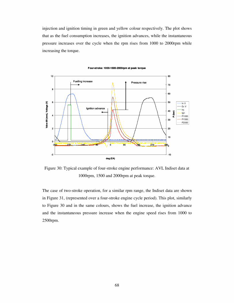
68
injection and ignition timing in green and yellow colour respectively. The plot shows
that as the fuel consumption increases, the ignition advances, while the instantaneous
pressure increases over the cycle when the rpm rises from 1000 to 2000rpm while
increasing the torque.
Figure 30: Typical example of four-stroke engine performance: AVL Indiset data at
1000rpm, 1500 and 2000rpm at peak torque.
The case of two-stroke operation, for a similar rpm range, the Indiset data are shown
in Figure 31, (represented over a four-stroke engine cycle period). This plot, similarly
to Figure 30 and in the same colours, shows the fuel increase, the ignition advance
and the instantaneous pressure increase when the engine speed rises from 1000 to
2500rpm.
Fuelling increase
Ignition advance
Pressure rise
Four-stroke: 1000-1500-2000rpm at peak torque
-2
0
2
4
6
8
10
-360 -270 -180 -90 0 90 180 270 360
deg (CA)
Valv
e lif
t (m
m),
Vo
lta
ge
(V
)
-10
0
10
20
30
40
50
60
70
80
P (
ba
r)
In V
Ex V
Inj
Ign
P1000
P1500
P2000
Fuelling increase
Ignition advance
Pressure rise
Four-stroke: 1000-1500-2000rpm at peak torque
-2
0
2
4
6
8
10
-360 -270 -180 -90 0 90 180 270 360
deg (CA)
Valv
e lif
t (m
m),
Vo
lta
ge
(V
)
-10
0
10
20
30
40
50
60
70
80
P (
ba
r)
In V
Ex V
Inj
Ign
P1000
P1500
P2000
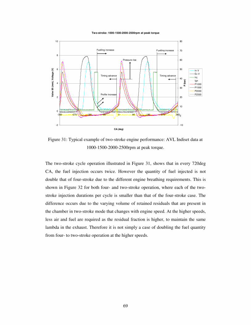
69
Figure 31: Typical example of two-stroke engine performance: AVL Indiset data at
1000-1500-2000-2500rpm at peak torque.
The two-stroke cycle operation illustrated in Figure 31, shows that in every 720deg
CA, the fuel injection occurs twice. However the quantity of fuel injected is not
double that of four-stroke due to the different engine breathing requirements. This is
shown in Figure 32 for both four- and two-stroke operation, where each of the two-
stroke injection durations per cycle is smaller than that of the four-stroke case. The
difference occurs due to the varying volume of retained residuals that are present in
the chamber in two-stroke mode that changes with engine speed. At the higher speeds,
less air and fuel are required as the residual fraction is higher, to maintain the same
lambda in the exhaust. Therefore it is not simply a case of doubling the fuel quantity
from four- to two-stroke operation at the higher speeds.
Two-stroke: 1000-1500-2000-2500rpm at peak torque
-2
0
2
4
6
8
10
-360 -270 -180 -90 0 90 180 270 360
CA (deg)
Va
lve
lif
t (m
m),
Vo
lta
ge (
V)
-10
0
10
20
30
40
50
60
70
80
P (
bar)
In V
Ex V
Inj
Ign
P1000
P1500
P2000
P2500
Fuelling increase
Timing advance
Profile increase
Pressure rise
Fuelling increase
Timing advance
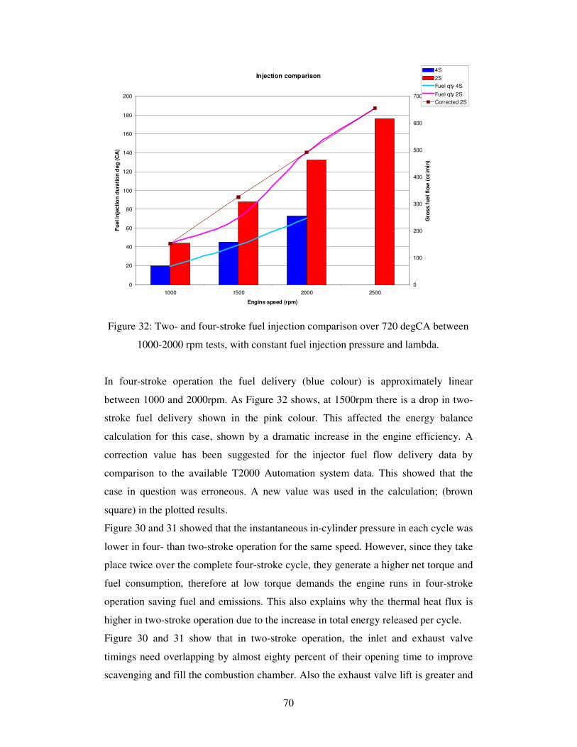
70
Figure 32: Two- and four-stroke fuel injection comparison over 720 degCA between
1000-2000 rpm tests, with constant fuel injection pressure and lambda.
In four-stroke operation the fuel delivery (blue colour) is approximately linear
between 1000 and 2000rpm. As Figure 32 shows, at 1500rpm there is a drop in two-
stroke fuel delivery shown in the pink colour. This affected the energy balance
calculation for this case, shown by a dramatic increase in the engine efficiency. A
correction value has been suggested for the injector fuel flow delivery data by
comparison to the available T2000 Automation system data. This showed that the
case in question was erroneous. A new value was used in the calculation; (brown
square) in the plotted results.
Figure 30 and 31 showed that the instantaneous in-cylinder pressure in each cycle was
lower in four- than two-stroke operation for the same speed. However, since they take
place twice over the complete four-stroke cycle, they generate a higher net torque and
fuel consumption, therefore at low torque demands the engine runs in four-stroke
operation saving fuel and emissions. This also explains why the thermal heat flux is
higher in two-stroke operation due to the increase in total energy released per cycle.
Figure 30 and 31 show that in two-stroke operation, the inlet and exhaust valve
timings need overlapping by almost eighty percent of their opening time to improve
scavenging and fill the combustion chamber. Also the exhaust valve lift is greater and
Injection comparison
0
20
40
60
80
100
120
140
160
180
200
1000 1500 2000 2500
Engine speed (rpm)
Fu
el in
jec
tio
n d
ura
tio
n d
eg
(C
A)
0
100
200
300
400
500
600
700
Gro
ss f
ue
l fl
ow
(cc
/min
)
4S
2S
Fuel qty 4S
Fuel qty 2S
Corrected 2S

71
the valve diameter is bigger than the inlet valve, to improve the scavenge process. The
timing variations affect the scavenging process and also the cylinder pressure results.
In addition the valve lift profile is not fixed over the two-stroke speed range. The
engine valve timing is fully variable and was optimized for each test case. Note, that
this variation is not included in the figures mentioned.
An important two-stroke requirement is that fuel injection takes place when both inlet
and exhaust valves are open, since there is not sufficient time for the fuel to be fully
mixed later in the cycle as in the four-stroke case.
For both two- and four-stroke, Figure 30 and 31 indicate the importance of the timing
of parameters upon the instantaneous pressure results. The correct combination results
in improved engine performance. Fine tuning of these parameters is specific for each
engine design and configuration and is particularly important in two-stroke operation.
The following was noted:
• Increasing the valve overlap generally leads to benefits from pulse effects.
Special attention is needed regarding piston to cylinder head clearance. In
addition, due to the lowered compression ratio, the inlet valve must close soon
after BDC, especially during cold start operation. Meanwhile idling and full
load operation are highly affected by the back flow (reverse) into the induction
manifold, together with the un-burnt mixture passing straight into the exhaust.
To further increase the flow, the inlet valve opens before TDC. In
turbocharged engines, this advance can be increased to improve the scavenge
effects. However during part load conditions, this may generate reverse flow
even in non turbocharged engines.
• Inlet valve closing takes place after BDC as there is still an incoming charge
due to the pressure difference in the combustion chamber.
• Expansion work is reduced by opening the exhaust valve early. Closing occurs
after TDC for high engine speeds and also for high boost pressures in
turbocharged engines. This avoids compressing the cylinder contents that will
produce back flow into the inlet manifold. However the engine may need a
compromise in timing between full- to part-load and high- to low-speed
performance.
• Generally the exhaust valves have a fixed opening time before BDC, ensuring
that the exhaust gases escape with no expense to the power stroke.
72
• With regards to short and long ignition coil charge duration, generally the
thermal conversion efficiency is better in short duration, when augmented by
in-cylinder motion through higher acceleration of the flame kernel which
normally generates a more stable combustion. Meanwhile, longer ignition
durations are also desirable, since they produce a greater operating window
that can cope with in-cylinder variations in AFR. It is also important to
consider that a large gap at the spark plug electrode can overcome a weak
mixture but is more sensitive to the turbulence and local mixture concentration
(Stone, (1999)).
Figure 33, shows the results of a simulation of the engine performed using the
Ricardo WAVE package (Ricardo, (2006)). Instantaneous pressure and temperature
for two-stroke operation are plotted against CA. The 1-D gas dynamics simulation
was performed using the in-cylinder pressure data collected during two-stroke engine
operation. The simulation, performed by Ricardo Consulting Engineers, was then
used to predict the evolution of the in-cylinder mean gas temperature. The results
were used in the energy balance (steady-state) calculation and in the comparison of
the 1-D heat flux correlations summarised in Appendix B.
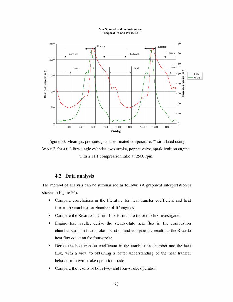
73
Figure 33: Mean gas pressure, pi and estimated temperature, Ti simulated using
WAVE, for a 0.3 litre single cylinder, two-stroke, poppet valve, spark ignition engine,
with a 11:1 compression ratio at 2500 rpm.
4.2 Data analysis
The method of analysis can be summarised as follows. (A graphical interpretation is
shown in Figure 34):
• Compare correlations in the literature for heat transfer coefficient and heat
flux in the combustion chamber of IC engines.
• Compare the Ricardo 1-D heat flux formula to those models investigated.
• Engine test results; derive the steady-state heat flux in the combustion
chamber walls in four-stroke operation and compare the results to the Ricardo
heat flux equation for four-stroke.
• Derive the heat transfer coefficient in the combustion chamber and the heat
flux, with a view to obtaining a better understanding of the heat transfer
behaviour in two-stroke operation mode.
• Compare the results of both two- and four-stroke operation.
One Dimensional Instantaneous
Temperature and Pressure
0
500
1000
1500
2000
2500
0 200 400 600 800 1000 1200 1400 1600 1800
CA (deg)
Me
an
ga
s t
em
pe
ratu
re (
K)
0
10
20
30
40
50
60
70
80
Me
an
ga
s p
ress
ure
(b
ar)
Ti (K)
Pi (bar)
ExhaustExhaust
Inlet Inlet
Burning Burning
Exhaust
Inlet
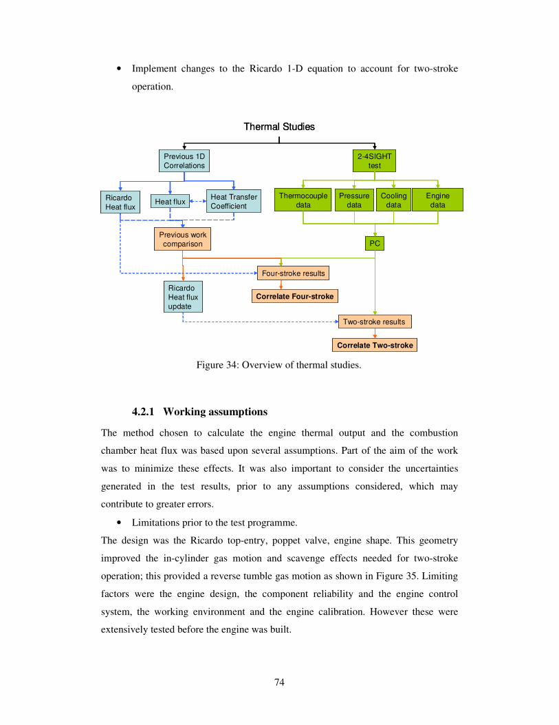
74
• Implement changes to the Ricardo 1-D equation to account for two-stroke
operation.
Figure 34: Overview of thermal studies.
4.2.1 Working assumptions
The method chosen to calculate the engine thermal output and the combustion
chamber heat flux was based upon several assumptions. Part of the aim of the work
was to minimize these effects. It was also important to consider the uncertainties
generated in the test results, prior to any assumptions considered, which may
contribute to greater errors.
• Limitations prior to the test programme.
The design was the Ricardo top-entry, poppet valve, engine shape. This geometry
improved the in-cylinder gas motion and scavenge effects needed for two-stroke
operation; this provided a reverse tumble gas motion as shown in Figure 35. Limiting
factors were the engine design, the component reliability and the engine control
system, the working environment and the engine calibration. However these were
extensively tested before the engine was built.
Thermal Studies
Four-stroke results
Previous work
comparison
Two-stroke results
2-4SIGHT
test
Cooling
data
Pressure
data
Thermocouple
data
PC
Engine
data
Previous 1D
Correlations
Heat fluxHeat Transfer
CoefficientRicardo
Heat flux
Ricardo
Heat flux
update
Correlate Four-stroke
Correlate Two-stroke
Thermal Studies
Four-stroke results
Previous work
comparison
Two-stroke results
2-4SIGHT
test
Cooling
data
Pressure
data
Thermocouple
data
PC
Engine
data
Previous 1D
Correlations
Heat fluxHeat Transfer
CoefficientRicardo
Heat flux
Ricardo
Heat flux
update
Correlate Four-stroke
Correlate Two-stroke
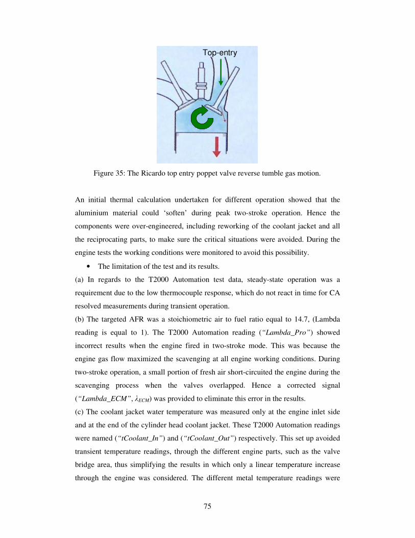
75
Figure 35: The Ricardo top entry poppet valve reverse tumble gas motion.
An initial thermal calculation undertaken for different operation showed that the
aluminium material could ‘soften’ during peak two-stroke operation. Hence the
components were over-engineered, including reworking of the coolant jacket and all
the reciprocating parts, to make sure the critical situations were avoided. During the
engine tests the working conditions were monitored to avoid this possibility.
• The limitation of the test and its results.
(a) In regards to the T2000 Automation test data, steady-state operation was a
requirement due to the low thermocouple response, which do not react in time for CA
resolved measurements during transient operation.
(b) The targeted AFR was a stoichiometric air to fuel ratio equal to 14.7, (Lambda
reading is equal to 1). The T2000 Automation reading (“Lambda_Pro”) showed
incorrect results when the engine fired in two-stroke mode. This was because the
engine gas flow maximized the scavenging at all engine working conditions. During
two-stroke operation, a small portion of fresh air short-circuited the engine during the
scavenging process when the valves overlapped. Hence a corrected signal
(“Lambda_ECM”, λECM) was provided to eliminate this error in the results.
(c) The coolant jacket water temperature was measured only at the engine inlet side
and at the end of the cylinder head coolant jacket. These T2000 Automation readings
were named (“tCoolant_In”) and (“tCoolant_Out”) respectively. This set up avoided
transient temperature readings, through the different engine parts, such as the valve
bridge area, thus simplifying the results in which only a linear temperature increase
through the engine was considered. The different metal temperature readings were
Top-entryTop-entry
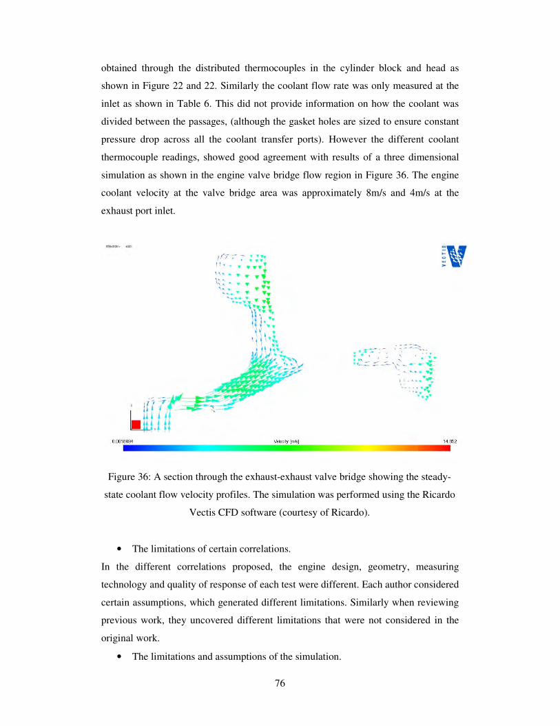
76
obtained through the distributed thermocouples in the cylinder block and head as
shown in Figure 22 and 22. Similarly the coolant flow rate was only measured at the
inlet as shown in Table 6. This did not provide information on how the coolant was
divided between the passages, (although the gasket holes are sized to ensure constant
pressure drop across all the coolant transfer ports). However the different coolant
thermocouple readings, showed good agreement with results of a three dimensional
simulation as shown in the engine valve bridge flow region in Figure 36. The engine
coolant velocity at the valve bridge area was approximately 8m/s and 4m/s at the
exhaust port inlet.
Figure 36: A section through the exhaust-exhaust valve bridge showing the steady-
state coolant flow velocity profiles. The simulation was performed using the Ricardo
Vectis CFD software (courtesy of Ricardo).
• The limitations of certain correlations.
In the different correlations proposed, the engine design, geometry, measuring
technology and quality of response of each test were different. Each author considered
certain assumptions, which generated different limitations. Similarly when reviewing
previous work, they uncovered different limitations that were not considered in the
original work.
• The limitations and assumptions of the simulation.
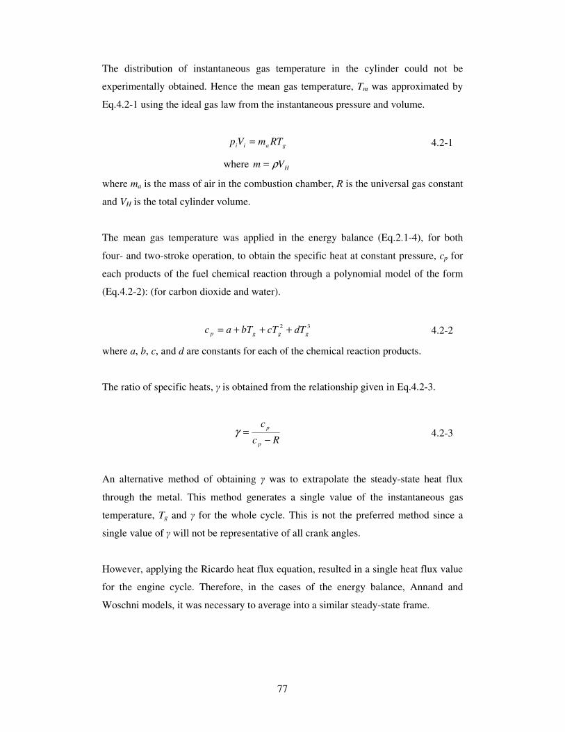
77
The distribution of instantaneous gas temperature in the cylinder could not be
experimentally obtained. Hence the mean gas temperature, Tm was approximated by
Eq.4.2-1 using the ideal gas law from the instantaneous pressure and volume.
gaii RTmVp = 4.2-1
where HVm ρ=
where ma is the mass of air in the combustion chamber, R is the universal gas constant
and VH is the total cylinder volume.
The mean gas temperature was applied in the energy balance (Eq.2.1-4), for both
four- and two-stroke operation, to obtain the specific heat at constant pressure, cp for
each products of the fuel chemical reaction through a polynomial model of the form
(Eq.4.2-2): (for carbon dioxide and water).
32
gggp dTcTbTac +++= 4.2-2
where a, b, c, and d are constants for each of the chemical reaction products.
The ratio of specific heats, γ is obtained from the relationship given in Eq.4.2-3.
Rc
c
p
p
−=γ 4.2-3
An alternative method of obtaining γ was to extrapolate the steady-state heat flux
through the metal. This method generates a single value of the instantaneous gas
temperature, Tg and γ for the whole cycle. This is not the preferred method since a
single value of γ will not be representative of all crank angles.
However, applying the Ricardo heat flux equation, resulted in a single heat flux value
for the engine cycle. Therefore, in the cases of the energy balance, Annand and
Woschni models, it was necessary to average into a similar steady-state frame.
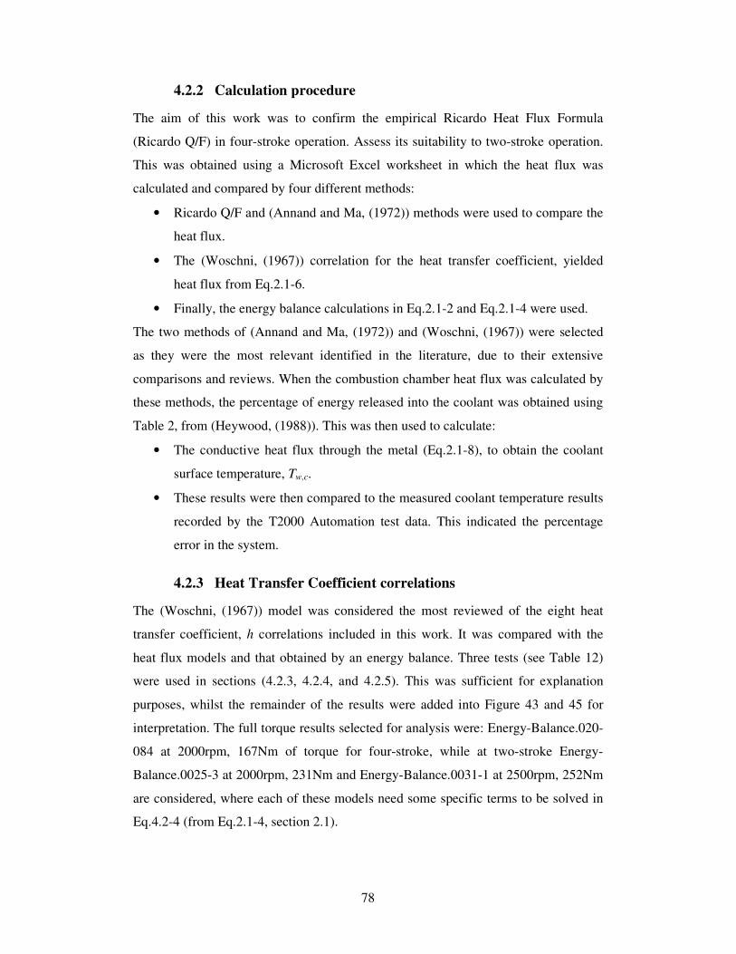
78
4.2.2 Calculation procedure
The aim of this work was to confirm the empirical Ricardo Heat Flux Formula
(Ricardo Q/F) in four-stroke operation. Assess its suitability to two-stroke operation.
This was obtained using a Microsoft Excel worksheet in which the heat flux was
calculated and compared by four different methods:
• Ricardo Q/F and (Annand and Ma, (1972)) methods were used to compare the
heat flux.
• The (Woschni, (1967)) correlation for the heat transfer coefficient, yielded
heat flux from Eq.2.1-6.
• Finally, the energy balance calculations in Eq.2.1-2 and Eq.2.1-4 were used.
The two methods of (Annand and Ma, (1972)) and (Woschni, (1967)) were selected
as they were the most relevant identified in the literature, due to their extensive
comparisons and reviews. When the combustion chamber heat flux was calculated by
these methods, the percentage of energy released into the coolant was obtained using
Table 2, from (Heywood, (1988)). This was then used to calculate:
• The conductive heat flux through the metal (Eq.2.1-8), to obtain the coolant
surface temperature, Tw,c.
• These results were then compared to the measured coolant temperature results
recorded by the T2000 Automation test data. This indicated the percentage
error in the system.
4.2.3 Heat Transfer Coefficient correlations
The (Woschni, (1967)) model was considered the most reviewed of the eight heat
transfer coefficient, h correlations included in this work. It was compared with the
heat flux models and that obtained by an energy balance. Three tests (see Table 12)
were used in sections (4.2.3, 4.2.4, and 4.2.5). This was sufficient for explanation
purposes, whilst the remainder of the results were added into Figure 43 and 45 for
interpretation. The full torque results selected for analysis were: Energy-Balance.020-
084 at 2000rpm, 167Nm of torque for four-stroke, while at two-stroke Energy-
Balance.0025-3 at 2000rpm, 231Nm and Energy-Balance.0031-1 at 2500rpm, 252Nm
are considered, where each of these models need some specific terms to be solved in
Eq.4.2-4 (from Eq.2.1-4, section 2.1).

79
θγθγ
γ
θ
δ
d
dpV
d
dVp
d
Qn
1
1
1 −+
−= 4.2-4
The four- and two-stroke energy balances are shown in Table 13 section (a) and (b)
respectively at full torque (80, 126 and 167Nm of torque in four-stroke, 136, 192, 231
and 252Nm in two-stroke) for 1000, 1500 and 2000rpm for both operations and
2500rpm case in two-stroke mode only.
4s (a)
Energy-Balance.020-091
qFuel_Mean 66.90 cc/min Tg max 2322.79 K
rpm 1000 Tg min 407.01 K
Total Energy 1393.94 J/cycle,cyl Tm 1384.73 K
Net heat release 823.11 J/cycle,cyl
Thermal Efficiency 59.05% Torque 80 Nm
Energy-Balance.017-087
qFuel_Mean 146.75 cc/min Tg max 3231.33 K
rpm 1500 Tg min 584.13 K
Total Energy 2038.58 J/cycle,cyl Tm 2009.75 K
Net heat release 1270.91 J/cycle,cyl
Thermal Efficiency 62.34% Torque 126 Nm
Energy-Balance.020-084
qFuel_Mean 246.20 cc/min Tg max 4124.69 K
rpm 2000 Tg min 718.54 K
Total Energy 2565.10 J/cycle,cyl Tm 2579.90 K
Net heat release 1723.33 J/cycle,cyl
Thermal Efficiency 67.18% Torque 167 Nm

80
2s (b)
Table 13: Energy balance results at full torque in:
(a) Four-stroke; 1000rpm, 80Nm; 1500 rpm, 126Nm; 2000rpm, 167Nm.
(b) Two-stroke; 1000rpm, 136Nm; 1500rpm, 192Nm; 2000rpm, 231Nm; 2500rpm,
252Nm.
Results from Table 13 show the net heat release results. The percentage of total
energy into the coolant is then taken from Table 2 (17-26% range at maximum power)
(Heywood, (1988)). The results are included in Figure 43 and 45 for four- and two-
stroke respectively.
For four-stroke operation, Woschni’s data is shown in Table 14 (a). The following
data was considered; temperature at start of ignition, T1, pressure at start of ignition,
p1, volume at start of ignition, V1 (from the Indiset data). The swirl coefficient term,
C1 and the gas velocity term, C2 are also included. The motored pressure, pom was
taken from data in Figure 37, (plot corresponds to the 24CAR-022, T2000
Automation test data which runs at motored conditions for the 24CAR-1022 Indiset
data at 2500rpm).
Energy-Balance.0025-1
qFuel_Mean 152.36 cc/min Tg max 2204.88 K
rpm 1000 Tg min 429.37 K
Total Energy 3174.75 J/cycle,cyl Tm 1391.66 K
Net heat release 1629.15 J/cycle,cyl
Thermal Efficiency 51.32% Torque 136 Nm
Energy-Balance.0025-2
qFuel_Mean 325.04 cc/min Tg max 2791.12 K
rpm 1500 Tg min 443.56 K
Total Energy 4515.27 J/cycle,cyl Tm 1689.80 K
Net heat release 2331.53 J/cycle,cyl
Thermal Efficiency 51.64% Torque 192 Nm
Energy-Balance.0025-3
qFuel_Mean 491.70 cc/min Tg max 3225.83 K
rpm 2000.00 Tg min 460.29 K
Total Energy 5122.81 J/cycle,cyl Tm 1944.43 K
Net heat release 2700.83 J/cycle,cyl
Thermal Efficiency 52.72% Torque 231 Nm
Energy-Balance.0031-1
qFuel_Mean 655.78 cc/min Tg max 3502.83 K
rpm 2500 Tg min 620.94 K
Total Energy 5465.83 J/cycle,cyl Tm 2072.84 K
Net heat release 2741.54 J/cycle,cylThermal Efficiency 50.16% Torque 252 Nm

81
4s (a)
2s (b)
2s (c)
TFS031-001, at 2500rpm and 252Nm
Term Value Units Effective range
T g K Instantaneous variation
p i bar File (Indiset TFS_0031-1)
C m 5.566667 m/s
p 1 11.677 bar
V 1 6.62E-05 m3
T 1 639.4359 K
p om bar File (Indiset TFS027-005 data set)
C 1 6.18 m/sK from -360 to -223.5, from -48.5 to 137, from 312 to 360 deg
C 1 2.28 m/sK from -223.5 to -48.5, from 137 to 312 deg
C 2 0 m/sK from -360 to -250.5, from -41.5 to 109.5, from 321 to 360 deg
C 2 3.40E-03 m/sK from -250.5 to -41.5, from 109.5 to 321 deg
TFS025-003, at 2000rpm and 231Nm
Term Value Units Effective range
T g K Instantaneous variation
p i bar File (Indiset TFS_0025-3)
C m 4.453 m/s
p 1 10.184 bar
V 1 6.62E-05 m3
T 1 557.6788 K
p om bar File (Indiset TFS027-005 data set)
C 1 6.18 m/sK from -360 to -244, from -38.5 to 114, from 316 to 360 deg
C 1 2.28 m/sK from -244 to -38.5, from 114 to 316 deg
C 2 0 m/sK from -360 to -271, from -14 to 89, from 345.5 to 360 deg
C 2 3.40E-03 m/sK from -271 to -14, from 89 to 345.5 deg
24CAR-084, at 2000rpm and 167Nm
Term Value Units Effective range
T g K Instantaneous variation
p i bar File (Indiset 24CAR-084)
C m 4.453 m/s
p 1 14.731 bar
V 1 6.8E-05 m3
T 1 829.4585 K
p om bar File (Indiset 24CAR-1022 data set)
C 1 6.18 m/sK from -360 to -122.5, from 340.5 to 360 deg
C 1 2.28 m/sK from -122.5 to 340.5 deg
C 2 0 m/sK from -360 to -18 deg
C 2 3.40E-03 m/sK from -18 to 360 deg
Common terms
Term Value Units Effective range
d 0.0816 m
m 0.8
V H 0.000349 m3
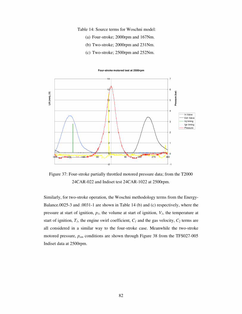
82
Table 14: Source terms for Woschni model:
(a) Four-stroke; 2000rpm and 167Nm.
(b) Two-stroke; 2000rpm and 231Nm.
(c) Two-stroke; 2500rpm and 252Nm.
Figure 37: Four-stroke partially throttled motored pressure data; from the T2000
24CAR-022 and Indiset test 24CAR-1022 at 2500rpm.
Similarly, for two-stroke operation, the Woschni methodology terms from the Energy-
Balance.0025-3 and .0031-1 are shown in Table 14 (b) and (c) respectively, where the
pressure at start of ignition, p1, the volume at start of ignition, V1, the temperature at
start of ignition, T1, the engine swirl coefficient, C1 and the gas velocity, C2 terms are
all considered in a similar way to the four-stroke case. Meanwhile the two-stroke
motored pressure, pom conditions are shown through Figure 38 from the TFS027-005
Indiset data at 2500rpm.
Four-stroke motored test at 2500rpm
-2
0
2
4
6
8
10
12
14
-360 -270 -180 -90 0 90 180 270 360
Lif
t (m
m),
(V
)
-1
0
1
2
3
4
5
6
7
Pre
ssu
re (
bar)
In Valve
Exh Valve
Inj timing
Ign timing
Pressure

83
Figure 38: Two-stroke partially throttled motored pressure data: from Indiset test
TFS027-005 at 2500rpm
The Woschni heat transfer coefficient, h in four-stroke operation at 2000rpm was
obtained from data in Figure 37, together with that of Table 14 (a) and Eq.4.2-5 (from
Eq.2.4-5 section 2.4.3). The results were converted into heat flux by averaging the
cycle results while applying Eq.4.2-6 (from Eq.2.1-6 section 2.1).
( )m
miH
m
m
g
m
i
mpp
Vp
TVCCCTpdh
−+= −−
0
11
121
62.175.01012592.0 4.2-5
( )wmi
ht TThAdt
Q−=
δ 4.2-6
Table 15 (a) shows the four-stroke energy balance heat flux results together with
those of (Woschni, (1967)); for 1000rpm and 80Nm of torque; 1500rpm and 126Nm;
and 2000rpm and 167Nm. The figures showed that the Woschni results were
consistently lower than the energy balance ones, while at higher engine speeds, the
difference in results became smaller. This is likely due to the combustion motion term
in the Woschni model; it may not have been accurately specified for low engine
Two-stroke motored test at 2500rpm
-2
0
2
4
6
8
10
-360 -260 -160 -60 40 140 240 340
CA (deg)
Lif
t (m
m),
(V
)
-0.5
0
0.5
1
1.5
2
2.5
3
Pre
ssu
re (
bar)
In Valve
Ex Valve
Inj timing
Ign timing
Pressure
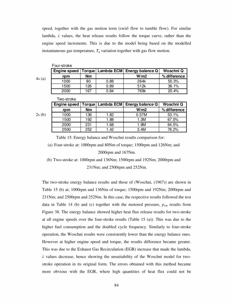
84
speed, together with the gas motion term (swirl flow to tumble flow). For similar
lambda, λ values, the heat release results follow the torque curve, rather than the
engine speed increments. This is due to the model being based on the modelled
instantaneous gas temperature, Tg variation together with gas flow motion.
4s (a)
2s (b)
Table 15: Energy balance and Woschni results comparison for:
(a) Four-stroke at: 1000rpm and 80Nm of torque; 1500rpm and 126Nm; and
2000rpm and 167Nm.
(b) Two-stroke at: 1000rpm and 136Nm; 1500rpm and 192Nm; 2000rpm and
231Nm; and 2500rpm and 252Nm.
The two-stroke energy balance results and those of (Woschni, (1967)) are shown in
Table 15 (b) at; 1000rpm and 136Nm of torque; 1500rpm and 192Nm; 2000rpm and
231Nm; and 2500rpm and 252Nm. In this case, the respective results followed the test
data in Table 14 (b) and (c) together with the motored pressure, pom results from
Figure 38. The energy balance showed higher heat flux release results for two-stroke
at all engine speeds over the four-stroke results (Table 15 (a)). This was due to the
higher fuel consumption and the doubled cycle frequency. Similarly to four-stroke
operation, the Woschni results were consistently lower than the energy balance ones.
However at higher engine speed and torque, the results difference became greater.
This was due to the Exhaust Gas Recirculation (EGR) increase that made the lambda,
λ values decrease, hence showing the unsuitability of the Woschni model for two-
stroke operation in its original form. The errors obtained with this method became
more obvious with the EGR, where high quantities of heat flux could not be
Two-stroke
Engine speed Torque Lambda ECM Energy balance Q Woschni Q
rpm Nm W/m2 % difference
1000 136 1.82 0.57M 53.1%
1500 192 1.88 1.3M 67.0%
2000 231 1.68 1.9M 64.5%
2500 252 1.42 3.4M 78.2%
Four-stroke
Engine speed Torque Lambda ECM Energy balance Q Woschni Q
rpm Nm W/m2 % difference
1000 80 0.88 264k 50.3%
1500 126 0.89 512k 36.1%
2000 167 0.84 769k 20.4%
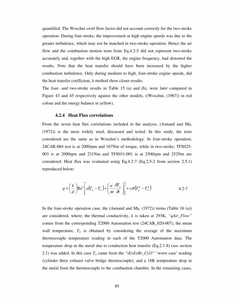
85
quantified. The Woschni swirl flow factor did not account correctly for the two-stroke
operation. During four-stroke, the improvement at high engine speeds was due to the
greater turbulence, which may not be matched in two-stroke operation. Hence the air
flow and the combustion motion term from Eq.4.2-5 did not represent two-stroke
accurately and, together with the high EGR, the engine frequency, had distorted the
results. Note that the heat transfer should have been increased by the higher
combustion turbulence. Only during medium to high, four-stroke engine speeds, did
the heat transfer coefficient, h method show closer results.
The four- and two-stroke results in Table 15 (a) and (b), were later compared in
Figure 43 and 45 respectively against the other models, ((Woschni, (1967)) in red
colour and the energy balance in yellow).
4.2.4 Heat Flux correlations
From the seven heat flux correlations included in the analysis, (Annand and Ma,
(1972)) is the most widely used, discussed and tested. In this study, the tests
considered are the same as in Woschni’s methodology. In four-stroke operation;
24CAR-084 test is at 2000rpm and 167Nm of torque, while in two-stroke; TFS025-
003 is at 2000rpm and 231Nm and TFS031-001 is at 2500rpm and 252Nm are
considered. Heat flux was evaluated using Eq.4.2-7 (Eq.2.5-2 from section 2.5.1)
reproduced below:
( ) ( )44'
Re wg
g
wg
bTTc
t
TaTTa
d
kq −+
+−
= σ
δ
δ
ω 4.2-7
In the four-stroke operation case, the (Annand and Ma, (1972)) terms (Table 16 (a))
are considered, where; the thermal conductivity, k is taken at 293K, ”qAir_Flow”
comes from the corresponding T2000 Automation test (24CAR_020-007), the mean
wall temperature, Tw is obtained by considering the average of the maximum
thermocouple temperature reading in each of the T2000 Automation data. The
temperature drop in the metal due to conduction heat transfer (Eq.2.1-8) (see section
2.1) was added. In this case Tw came from the “tExExBr_Cyl3” ‘worst case’ reading
(cylinder three exhaust valve bridge thermocouple), and a 18K temperature drop in
the metal from the thermocouple to the combustion chamber. In the remaining cases,
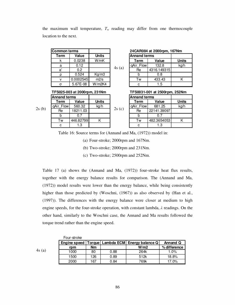
86
the maximum wall temperature, Tw reading may differ from one thermocouple
location to the next.
4s (a)
2s (b)
2s (c)
Table 16: Source terms for (Annand and Ma, (1972)) model in:
(a) Four-stroke; 2000rpm and 167Nm.
(b) Two-stroke; 2000rpm and 231Nm.
(c) Two-stroke; 2500rpm and 252Nm.
Table 17 (a) shows the (Annand and Ma, (1972)) four-stroke heat flux results,
together with the energy balance results for comparison. The (Annand and Ma,
(1972)) model results were lower than the energy balance, while being consistently
higher than those predicted by (Woschni, (1967)) as also observed by (Han et al.,
(1997)). The differences with the energy balance were closer at medium to high
engine speeds, for the four-stroke operation, with constant lambda, λ readings. On the
other hand, similarly to the Woschni case, the Annand and Ma results followed the
torque trend rather than the engine speed.
4s (a)
Four-stroke
Engine speed Torque Lambda ECM Energy balance Q Annand Q
rpm Nm W/m2 % difference1000 80 0.88 264k 1.0%
1500 126 0.89 512k 18.8%
2000 167 0.84 769k 17.0%
TFS0031-001 at 2500rpm, 252Nm
Annand terms
Term Value Units
qAir_Flow 681.25 kg/h
Re 22141.39097
b 0.7
Tw 482.3654053 K
c 1.3
TFS025-003 at 2000rpm, 231Nm
Annand terms
Term Value Units
qAir_Flow 560.32 kg/h
Re 18211.03
b 0.7
Tw 446.82799 K
c 1.3
24CAR084 at 2000rpm, 167Nm
Annand terms
Term Value Units
qAir_Flow 132.8 kg/h
Re 4316.149315
b 0.8
Tw 433.43 K
c 1.5
Common terms
Term Value Units
k 0.0238 W/mK
a 0.12
a' 0.2
ρ 0.524 Kg/m3
v 0.0002545 m2/s
σ 5.67E-08 W/m2K4

87
2s (b)
Table 17: Energy balance and Annand and Ma model results comparison in:
(a) Four-stroke at 1000rpm and 80Nm of torque, 1500rpm and 126Nm and 2000rpm
and 167Nm.
(b) Two-stroke at 1000rpm and 136Nm, 1500rpm and 192Nm, 2000rpm and 231Nm
and 2500rpm and 252Nm.
For two-stroke operation, the parameters are shown in Table 16 (b) for the 2000rpm,
231Nm of torque; and 2500rpm 252Nm cases respectively. The TFS025-003
(2000rpm and 231Nm of torque) thermocouple reading case is “tUTRRP_Ex_Cyl3”
(upper top reversal point in exhaust for cylinder three) and “tExExBr_Cyl2” (exhaust
valve bridge for cylinder two) for TFS031-001 (2500rpm at 252Nm) case. The two-
stroke constants that differ from those of the four-stroke operation ones are: Reynolds
number exponent, b and the radiation coefficient for combustion and expansion
strokes term, c only.
(Annand and Ma, (1972)) two-stroke heat flux results in Table 17 (b) are higher than
those predicted by (Woschni, (1967)). This difference became smaller at the higher
engine speeds due to the increased gas flow motion in the Reynolds number, Re,
rather than by the instantaneous gas temperature, Tg difference. This is confirmed at
low engine speeds, where there was more time for the heat release to take place. The
four-stroke operation results were closer to those of the energy balance, than the
Woschni cases, also the case in two-stroke operation. However due to the higher
EGR, the results were affected. This was noticed in that the margin of difference in
the results over the engine speed range was closer than four-stroke operation. These
suggested that in case of no EGR, the results would have been closer to the energy
balance cases. The Woschni results were lower, due to the greater influence of the
instantaneous gas temperature, Tg, which in the Annand and Ma model, was further
affected by the Reynolds number dependancy.
Similarly to the Woschni results, the Annand and Ma four- and two-stroke results,
were compared in Figure 43 and 45 respectively, against the other models ((Woschni,
Two-stroke
Engine speed Torque Lambda ECM Energy balance Q Annand Q
rpm Nm W/m2 % difference
1000 136 1.82 0.57M 41.3%
1500 192 1.88 1.3M 49.9%
2000 231 1.68 1.9M 38.2%
2500 252 1.42 3.4M 50.8%
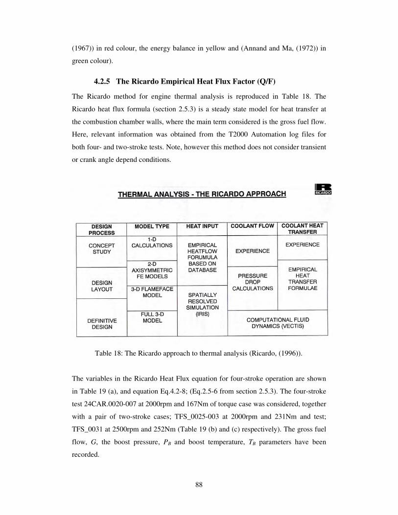
88
(1967)) in red colour, the energy balance in yellow and (Annand and Ma, (1972)) in
green colour).
4.2.5 The Ricardo Empirical Heat Flux Factor (Q/F)
The Ricardo method for engine thermal analysis is reproduced in Table 18. The
Ricardo heat flux formula (section 2.5.3) is a steady state model for heat transfer at
the combustion chamber walls, where the main term considered is the gross fuel flow.
Here, relevant information was obtained from the T2000 Automation log files for
both four- and two-stroke tests. Note, however this method does not consider transient
or crank angle depend conditions.
Table 18: The Ricardo approach to thermal analysis (Ricardo, (1996)).
The variables in the Ricardo Heat Flux equation for four-stroke operation are shown
in Table 19 (a), and equation Eq.4.2-8; (Eq.2.5-6 from section 2.5.3). The four-stroke
test 24CAR.0020-007 at 2000rpm and 167Nm of torque case was considered, together
with a pair of two-stroke cases; TFS_0025-003 at 2000rpm and 231Nm and test;
TFS_0031 at 2500rpm and 252Nm (Table 19 (b) and (c) respectively). The gross fuel
flow, G, the boost pressure, PB and boost temperature, TB parameters have been
recorded.
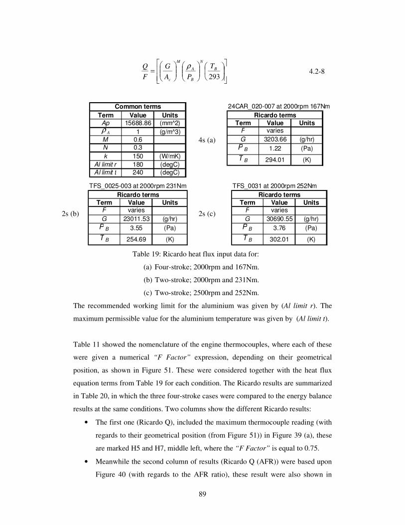
89
=
293
B
N
B
A
M
c
T
PA
G
F
Q ρ 4.2-8
4s (a)
2s (b)
2s (c)
Table 19: Ricardo heat flux input data for:
(a) Four-stroke; 2000rpm and 167Nm.
(b) Two-stroke; 2000rpm and 231Nm.
(c) Two-stroke; 2500rpm and 252Nm.
The recommended working limit for the aluminium was given by (Al limit r). The
maximum permissible value for the aluminium temperature was given by (Al limit t).
Table 11 showed the nomenclature of the engine thermocouples, where each of these
were given a numerical “F Factor” expression, depending on their geometrical
position, as shown in Figure 51. These were considered together with the heat flux
equation terms from Table 19 for each condition. The Ricardo results are summarized
in Table 20, in which the three four-stroke cases were compared to the energy balance
results at the same conditions. Two columns show the different Ricardo results:
• The first one (Ricardo Q), included the maximum thermocouple reading (with
regards to their geometrical position (from Figure 51)) in Figure 39 (a), these
are marked H5 and H7, middle left, where the “F Factor” is equal to 0.75.
• Meanwhile the second column of results (Ricardo Q (AFR)) were based upon
Figure 40 (with regards to the AFR ratio), these result were also shown in
TFS_0025-003 at 2000rpm 231Nm
Term Value UnitsF varies
G 23011.53 (g/hr)
P B 3.55 (Pa)
T B 254.69 (K)
Ricardo terms
Term Value UnitsAp 15688.86 (mm^2)
1 (g/m^3)
M 0.6
N 0.3
k 150 (W/mK)
Al limit r 180 (degC)
Al limit t 240 (degC)
Common terms
Aρ
TFS_0031 at 2000rpm 252Nm
Term Value UnitsF varies
G 30690.55 (g/hr)
P B 3.76 (Pa)
T B 302.01 (K)
Ricardo terms
24CAR_020-007 at 2000rpm 167Nm
Term Value UnitsF varies
G 3203.66 (g/hr)
P B 1.22 (Pa)
T B 294.01 (K)
Ricardo terms
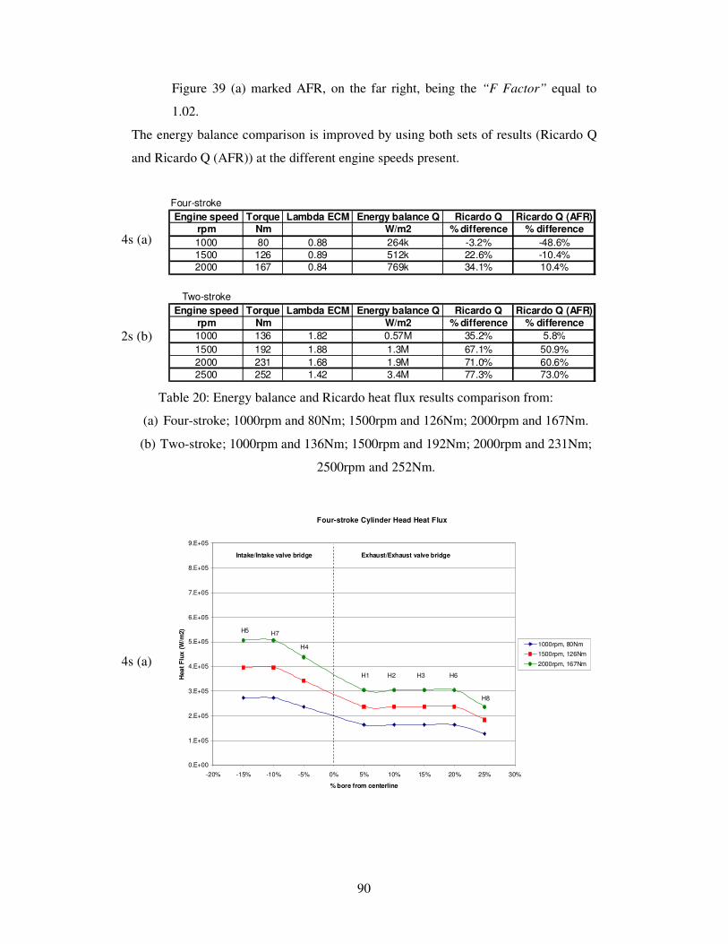
90
Figure 39 (a) marked AFR, on the far right, being the “F Factor” equal to
1.02.
The energy balance comparison is improved by using both sets of results (Ricardo Q
and Ricardo Q (AFR)) at the different engine speeds present.
4s (a)
2s (b)
Table 20: Energy balance and Ricardo heat flux results comparison from:
(a) Four-stroke; 1000rpm and 80Nm; 1500rpm and 126Nm; 2000rpm and 167Nm.
(b) Two-stroke; 1000rpm and 136Nm; 1500rpm and 192Nm; 2000rpm and 231Nm;
2500rpm and 252Nm.
4s (a)
Four-stroke Cylinder Head Heat Flux
0.E+00
1.E+05
2.E+05
3.E+05
4.E+05
5.E+05
6.E+05
7.E+05
8.E+05
9.E+05
-20% -15% -10% -5% 0% 5% 10% 15% 20% 25% 30%
% bore from centerline
Hea
t F
lux
(W
/m2)
1000rpm, 80Nm
1500rpm, 126Nm
2000rpm, 167Nm
Exhaust/Exhaust valve bridgeIntake/Intake valve bridge
H5 H7
H4
H1 H2 H3 H6
H8
Two-stroke
Engine speed Torque Lambda ECM Energy balance Q Ricardo Q Ricardo Q (AFR)
rpm Nm W/m2 % difference % difference
1000 136 1.82 0.57M 35.2% 5.8%
1500 192 1.88 1.3M 67.1% 50.9%
2000 231 1.68 1.9M 71.0% 60.6%
2500 252 1.42 3.4M 77.3% 73.0%
Four-stroke
Engine speed Torque Lambda ECM Energy balance Q Ricardo Q Ricardo Q (AFR)
rpm Nm W/m2 % difference % difference
1000 80 0.88 264k -3.2% -48.6%
1500 126 0.89 512k 22.6% -10.4%
2000 167 0.84 769k 34.1% 10.4%
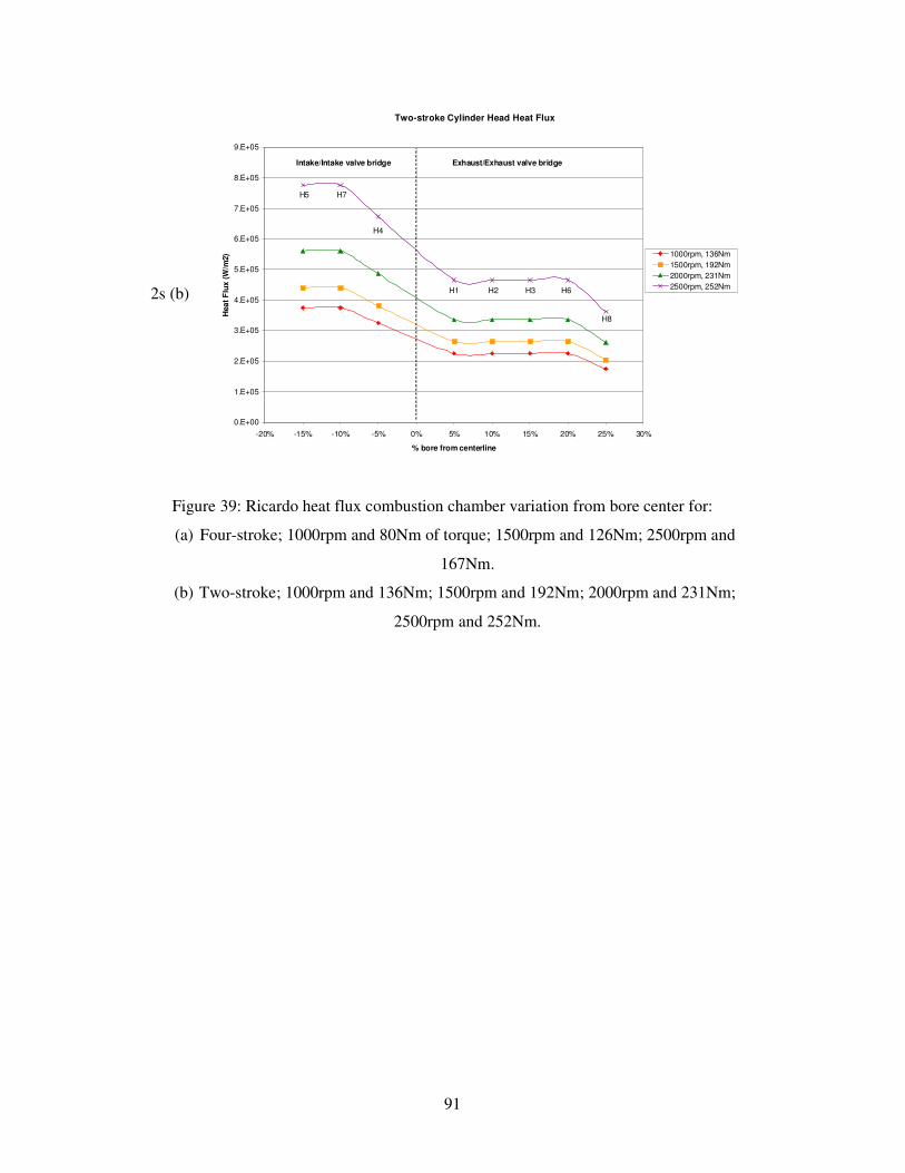
91
2s (b)
Figure 39: Ricardo heat flux combustion chamber variation from bore center for:
(a) Four-stroke; 1000rpm and 80Nm of torque; 1500rpm and 126Nm; 2500rpm and
167Nm.
(b) Two-stroke; 1000rpm and 136Nm; 1500rpm and 192Nm; 2000rpm and 231Nm;
2500rpm and 252Nm.
Two-stroke Cylinder Head Heat Flux
0.E+00
1.E+05
2.E+05
3.E+05
4.E+05
5.E+05
6.E+05
7.E+05
8.E+05
9.E+05
-20% -15% -10% -5% 0% 5% 10% 15% 20% 25% 30%
% bore from centerline
Hea
t F
lux
(W
/m2) 1000rpm, 136Nm
1500rpm, 192Nm
2000rpm, 231Nm
2500rpm, 252Nm
Exhaust/Exhaust valve bridgeIntake/Intake valve bridge
H5 H7
H4
H1 H2 H3 H6
H8
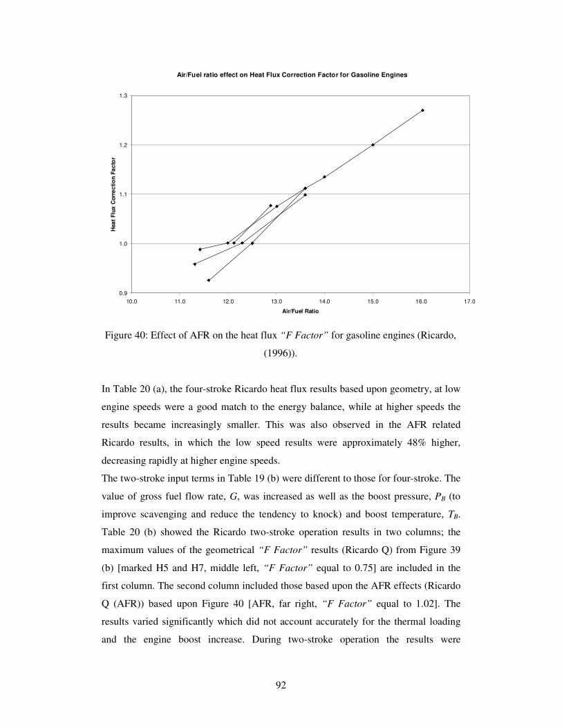
92
Figure 40: Effect of AFR on the heat flux “F Factor” for gasoline engines (Ricardo,
(1996)).
In Table 20 (a), the four-stroke Ricardo heat flux results based upon geometry, at low
engine speeds were a good match to the energy balance, while at higher speeds the
results became increasingly smaller. This was also observed in the AFR related
Ricardo results, in which the low speed results were approximately 48% higher,
decreasing rapidly at higher engine speeds.
The two-stroke input terms in Table 19 (b) were different to those for four-stroke. The
value of gross fuel flow rate, G, was increased as well as the boost pressure, PB (to
improve scavenging and reduce the tendency to knock) and boost temperature, TB.
Table 20 (b) showed the Ricardo two-stroke operation results in two columns; the
maximum values of the geometrical “F Factor” results (Ricardo Q) from Figure 39
(b) [marked H5 and H7, middle left, “F Factor” equal to 0.75] are included in the
first column. The second column included those based upon the AFR effects (Ricardo
Q (AFR)) based upon Figure 40 [AFR, far right, “F Factor” equal to 1.02]. The
results varied significantly which did not account accurately for the thermal loading
and the engine boost increase. During two-stroke operation the results were
Air/Fuel ratio effect on Heat Flux Correction Factor for Gasoline Engines
0.9
1.0
1.1
1.2
1.3
10.0 11.0 12.0 13.0 14.0 15.0 16.0 17.0
Air/Fuel Ratio
Hea
t F
lux
Co
rre
cti
on
Fa
cto
r
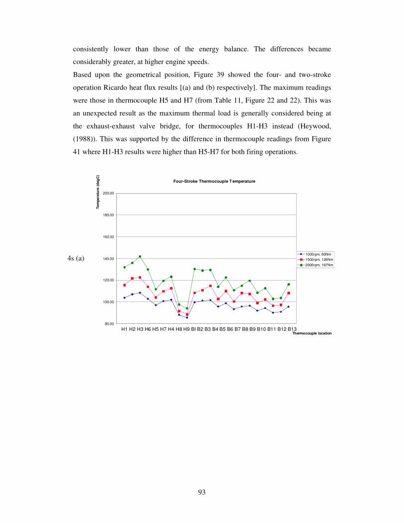
93
consistently lower than those of the energy balance. The differences became
considerably greater, at higher engine speeds.
Based upon the geometrical position, Figure 39 showed the four- and two-stroke
operation Ricardo heat flux results [(a) and (b) respectively]. The maximum readings
were those in thermocouple H5 and H7 (from Table 11, Figure 22 and 22). This was
an unexpected result as the maximum thermal load is generally considered being at
the exhaust-exhaust valve bridge, for thermocouples H1-H3 instead (Heywood,
(1988)). This was supported by the difference in thermocouple readings from Figure
41 where H1-H3 results were higher than H5-H7 for both firing operations.
4s (a)
H1 H2 H3 H6 H5 H7 H4 H8 H9 BI B2 B3 B4 B5 B6 B7 B8 B9 B10 B11 B12 B13
Four-Stroke Thermocouple T emperature
80.00
100.00
120.00
140.00
160.00
180.00
200.00
Thermocouple location
Te
mp
era
ture
(d
eg
C)
1000rpm, 80Nm
1500rpm, 126Nm
2000rpm, 167Nm

94
2s (b)
Figure 41: Full torque thermocouple temperature for:
(a) Four-stroke; 1000rpm and 80Nm; 1500rpm and 126Nm; 2000rpm and 167Nm.
(b) Two-stroke; 1000rpm and 136Nm; 1500rpm and 192Nm; 2000rpm and 231Nm;
2500rpm and 252Nm.
The EGR affected the two-stroke operation heat flux results. Table 20 showed this in
two ways:
A; the difference in results between the energy balance and the Ricardo heat flux
results for each firing operation.
B; the difference obtained between the four- and two-stroke operation
“lambda_ECM” results. Where the four-stroke results showed that this difference
would have been reduced if there were no EGR.
The Ricardo heat flux method, scaled linearly with the “F Factor”. This did not
account accurately for the in cylinder air flow and the turbulence difference. This
suggested that the two-stroke operation results would need to be corrected. The
differences between the two firing operations proved that during four-stroke
operation, the results could be improved if:
(1) At low engine speeds; a geometrical “F Factor” correction ((Ricardo Q) result
from Table 20 (a)) was considered.
Two-Stroke Thermocouple Temperature
80.00
100.00
120.00
140.00
160.00
180.00
200.00
Thermocouple Position
Te
mp
era
ture
(d
eg
C)
1000rpm, 136Nm
1500rpm, 192Nm
2000rpm, 231Nm
2500rpm, 252Nm
H1 H2 H3 H6 H5 H7 H4 H8 H9 BI B2 B3 B4 B5 B6 B7 B8 B9 B10 B11 B12 B13
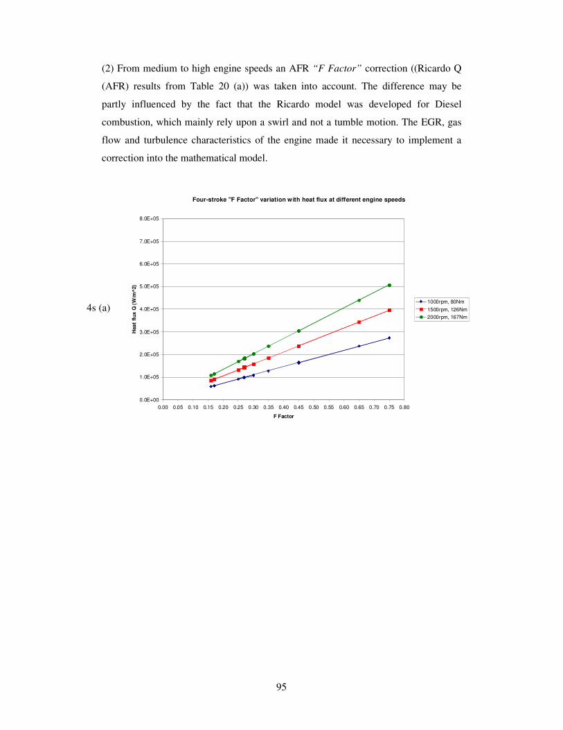
95
(2) From medium to high engine speeds an AFR “F Factor” correction ((Ricardo Q
(AFR) results from Table 20 (a)) was taken into account. The difference may be
partly influenced by the fact that the Ricardo model was developed for Diesel
combustion, which mainly rely upon a swirl and not a tumble motion. The EGR, gas
flow and turbulence characteristics of the engine made it necessary to implement a
correction into the mathematical model.
4s (a)
Four-stroke "F Factor" variation with heat flux at different engine speeds
0.0E+00
1.0E+05
2.0E+05
3.0E+05
4.0E+05
5.0E+05
6.0E+05
7.0E+05
8.0E+05
0.00 0.05 0.10 0.15 0.20 0.25 0.30 0.35 0.40 0.45 0.50 0.55 0.60 0.65 0.70 0.75 0.80
F Factor
Hea
t fl
ux
Q (
W/m
^2)
1000rpm, 80Nm
1500rpm, 126Nm
2000rpm, 167Nm
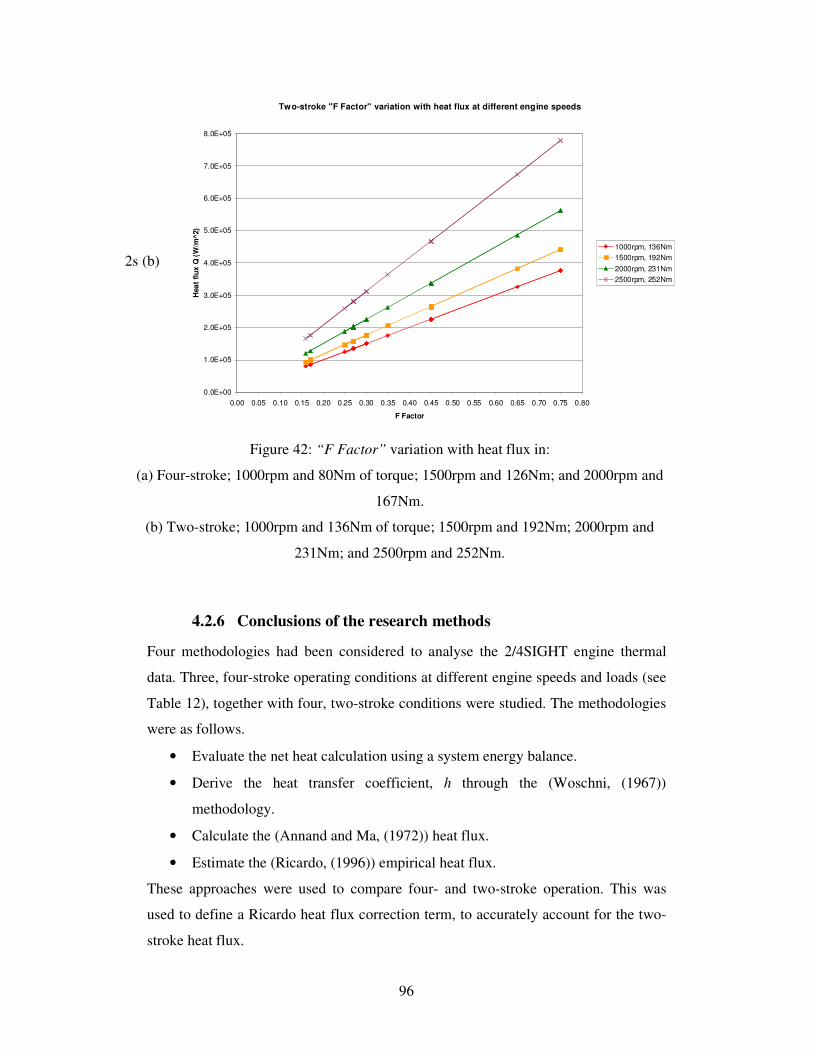
96
2s (b)
Figure 42: “F Factor” variation with heat flux in:
(a) Four-stroke; 1000rpm and 80Nm of torque; 1500rpm and 126Nm; and 2000rpm and
167Nm.
(b) Two-stroke; 1000rpm and 136Nm of torque; 1500rpm and 192Nm; 2000rpm and
231Nm; and 2500rpm and 252Nm.
4.2.6 Conclusions of the research methods
Four methodologies had been considered to analyse the 2/4SIGHT engine thermal
data. Three, four-stroke operating conditions at different engine speeds and loads (see
Table 12), together with four, two-stroke conditions were studied. The methodologies
were as follows.
• Evaluate the net heat calculation using a system energy balance.
• Derive the heat transfer coefficient, h through the (Woschni, (1967))
methodology.
• Calculate the (Annand and Ma, (1972)) heat flux.
• Estimate the (Ricardo, (1996)) empirical heat flux.
These approaches were used to compare four- and two-stroke operation. This was
used to define a Ricardo heat flux correction term, to accurately account for the two-
stroke heat flux.
Two-stroke "F Factor" variation with heat flux at different engine speeds
0.0E+00
1.0E+05
2.0E+05
3.0E+05
4.0E+05
5.0E+05
6.0E+05
7.0E+05
8.0E+05
0.00 0.05 0.10 0.15 0.20 0.25 0.30 0.35 0.40 0.45 0.50 0.55 0.60 0.65 0.70 0.75 0.80
F Factor
Hea
t fl
ux
Q (
W/m
^2)
1000rpm, 136Nm
1500rpm, 192Nm
2000rpm, 231Nm
2500rpm, 252Nm
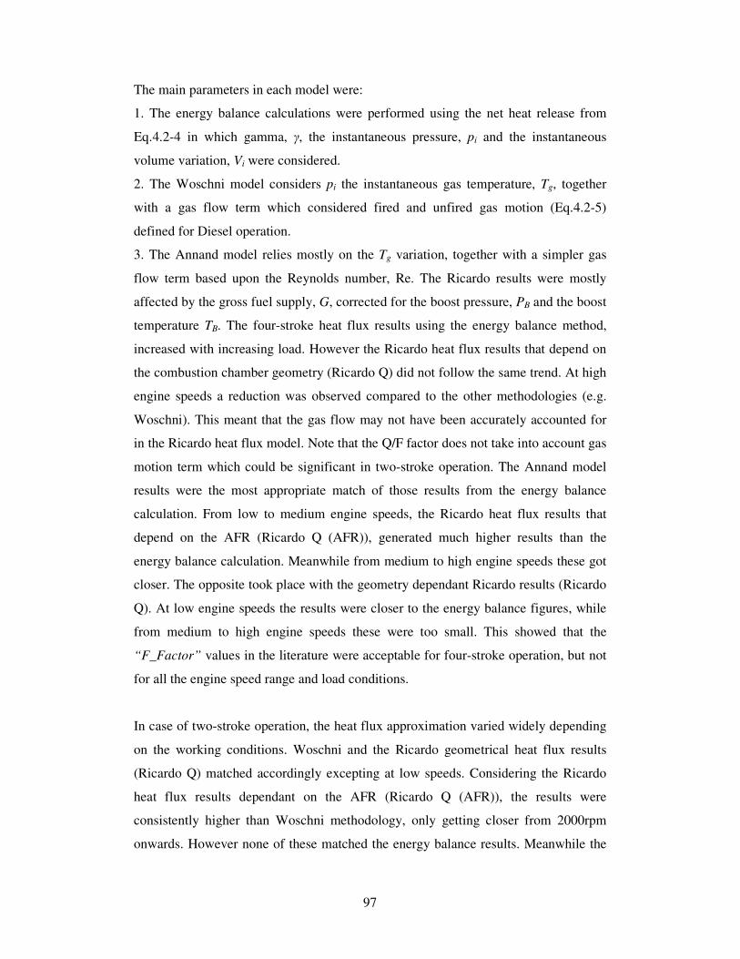
97
The main parameters in each model were:
1. The energy balance calculations were performed using the net heat release from
Eq.4.2-4 in which gamma, γ, the instantaneous pressure, pi and the instantaneous
volume variation, Vi were considered.
2. The Woschni model considers pi the instantaneous gas temperature, Tg, together
with a gas flow term which considered fired and unfired gas motion (Eq.4.2-5)
defined for Diesel operation.
3. The Annand model relies mostly on the Tg variation, together with a simpler gas
flow term based upon the Reynolds number, Re. The Ricardo results were mostly
affected by the gross fuel supply, G, corrected for the boost pressure, PB and the boost
temperature TB. The four-stroke heat flux results using the energy balance method,
increased with increasing load. However the Ricardo heat flux results that depend on
the combustion chamber geometry (Ricardo Q) did not follow the same trend. At high
engine speeds a reduction was observed compared to the other methodologies (e.g.
Woschni). This meant that the gas flow may not have been accurately accounted for
in the Ricardo heat flux model. Note that the Q/F factor does not take into account gas
motion term which could be significant in two-stroke operation. The Annand model
results were the most appropriate match of those results from the energy balance
calculation. From low to medium engine speeds, the Ricardo heat flux results that
depend on the AFR (Ricardo Q (AFR)), generated much higher results than the
energy balance calculation. Meanwhile from medium to high engine speeds these got
closer. The opposite took place with the geometry dependant Ricardo results (Ricardo
Q). At low engine speeds the results were closer to the energy balance figures, while
from medium to high engine speeds these were too small. This showed that the
“F_Factor” values in the literature were acceptable for four-stroke operation, but not
for all the engine speed range and load conditions.
In case of two-stroke operation, the heat flux approximation varied widely depending
on the working conditions. Woschni and the Ricardo geometrical heat flux results
(Ricardo Q) matched accordingly excepting at low speeds. Considering the Ricardo
heat flux results dependant on the AFR (Ricardo Q (AFR)), the results were
consistently higher than Woschni methodology, only getting closer from 2000rpm
onwards. However none of these matched the energy balance results. Meanwhile the
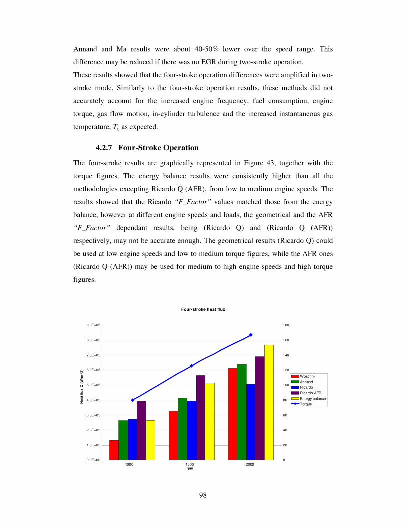
98
Annand and Ma results were about 40-50% lower over the speed range. This
difference may be reduced if there was no EGR during two-stroke operation.
These results showed that the four-stroke operation differences were amplified in two-
stroke mode. Similarly to the four-stroke operation results, these methods did not
accurately account for the increased engine frequency, fuel consumption, engine
torque, gas flow motion, in-cylinder turbulence and the increased instantaneous gas
temperature, Tg as expected.
4.2.7 Four-Stroke Operation
The four-stroke results are graphically represented in Figure 43, together with the
torque figures. The energy balance results were consistently higher than all the
methodologies excepting Ricardo Q (AFR), from low to medium engine speeds. The
results showed that the Ricardo “F_Factor” values matched those from the energy
balance, however at different engine speeds and loads, the geometrical and the AFR
“F_Factor” dependant results, being (Ricardo Q) and (Ricardo Q (AFR))
respectively, may not be accurate enough. The geometrical results (Ricardo Q) could
be used at low engine speeds and low to medium torque figures, while the AFR ones
(Ricardo Q (AFR)) may be used for medium to high engine speeds and high torque
figures.
Four-stroke heat flux
0.0E+00
1.0E+05
2.0E+05
3.0E+05
4.0E+05
5.0E+05
6.0E+05
7.0E+05
8.0E+05
9.0E+05
rpm
Hea
t fl
ux
Q (
W/m
^2
)
0
20
40
60
80
100
120
140
160
180
To
rqu
e (
Nm
)
Woschni
Annand
Ricardo
Ricardo AFR
Energy balance
Torque
1000 1500 2000
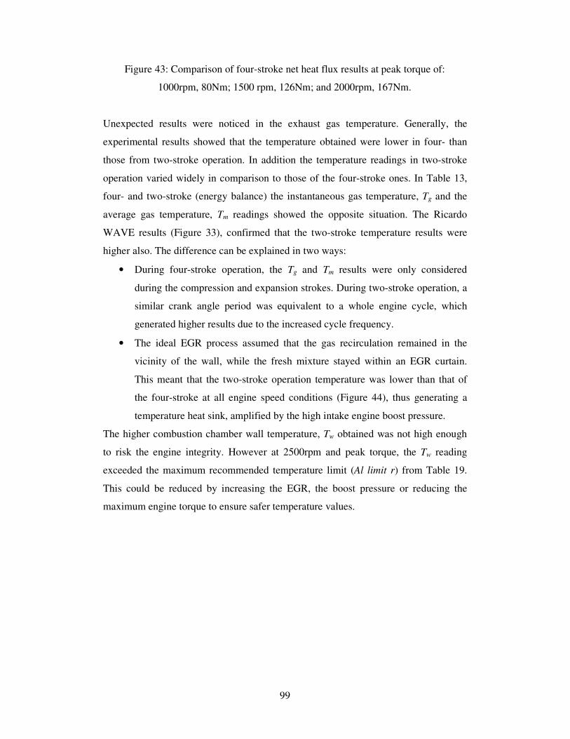
99
Figure 43: Comparison of four-stroke net heat flux results at peak torque of:
1000rpm, 80Nm; 1500 rpm, 126Nm; and 2000rpm, 167Nm.
Unexpected results were noticed in the exhaust gas temperature. Generally, the
experimental results showed that the temperature obtained were lower in four- than
those from two-stroke operation. In addition the temperature readings in two-stroke
operation varied widely in comparison to those of the four-stroke ones. In Table 13,
four- and two-stroke (energy balance) the instantaneous gas temperature, Tg and the
average gas temperature, Tm readings showed the opposite situation. The Ricardo
WAVE results (Figure 33), confirmed that the two-stroke temperature results were
higher also. The difference can be explained in two ways:
• During four-stroke operation, the Tg and Tm results were only considered
during the compression and expansion strokes. During two-stroke operation, a
similar crank angle period was equivalent to a whole engine cycle, which
generated higher results due to the increased cycle frequency.
• The ideal EGR process assumed that the gas recirculation remained in the
vicinity of the wall, while the fresh mixture stayed within an EGR curtain.
This meant that the two-stroke operation temperature was lower than that of
the four-stroke at all engine speed conditions (Figure 44), thus generating a
temperature heat sink, amplified by the high intake engine boost pressure.
The higher combustion chamber wall temperature, Tw obtained was not high enough
to risk the engine integrity. However at 2500rpm and peak torque, the Tw reading
exceeded the maximum recommended temperature limit (Al limit r) from Table 19.
This could be reduced by increasing the EGR, the boost pressure or reducing the
maximum engine torque to ensure safer temperature values.
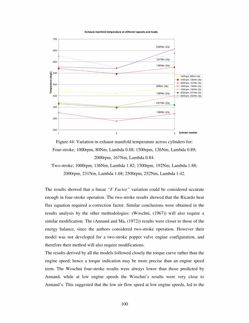
100
Figure 44: Variation in exhaust manifold temperature across cylinders for:
Four-stroke; 1000rpm, 80Nm, Lambda 0.88; 1500rpm, 126Nm, Lambda 0.89;
2000rpm, 167Nm, Lambda 0.84.
Two-stroke; 1000rpm, 136Nm, Lambda 1.82; 1500rpm, 192Nm, Lambda 1.88;
2000rpm, 231Nm, Lambda 1.68; 2500rpm, 252Nm, Lambda 1.42.
The results showed that a linear “F Factor” variation could be considered accurate
enough in four-stroke operation. The two-stroke results showed that the Ricardo heat
flux equation required a correction factor. Similar conclusions were obtained in the
results analysis by the other methodologies: (Woschni, (1967)) will also require a
similar modification. The (Annand and Ma, (1972)) results were closer to those of the
energy balance, since the authors considered two-stroke operation. However their
model was not developed for a two-stroke poppet valve engine configuration, and
therefore their method will also require modifications.
The results derived by all the models followed closely the torque curve rather than the
engine speed; hence a torque indication may be more precise than an engine speed
term. The Woschni four-stroke results were always lower than those predicted by
Annand, while at low engine speeds the Woschni’s results were very close to
Annand’s. This suggested that the low air flow speed at low engine speeds, led to the
Exhaust manifold temperature at different speeds and loads
300
350
400
450
500
550
600
650
700
1 2 3 Cylinder number
Tem
pe
ratu
re (
de
gC
)
1000rpm, 80Nm (4s)
1500rpm, 126Nm (4s)
2000rpm, 167Nm (4s)
1000rpm, 136Nm (2s)
1500rpm, 192Nm (2s)
2000rpm, 231Nm (2s)
2500rpm, 252Nm (2s)
252Nm (2s)
167Nm (4s)
126Nm (4s)
80Nm (4s)
192Nm (2s)
231Nm (2s)
136Nm (2s)
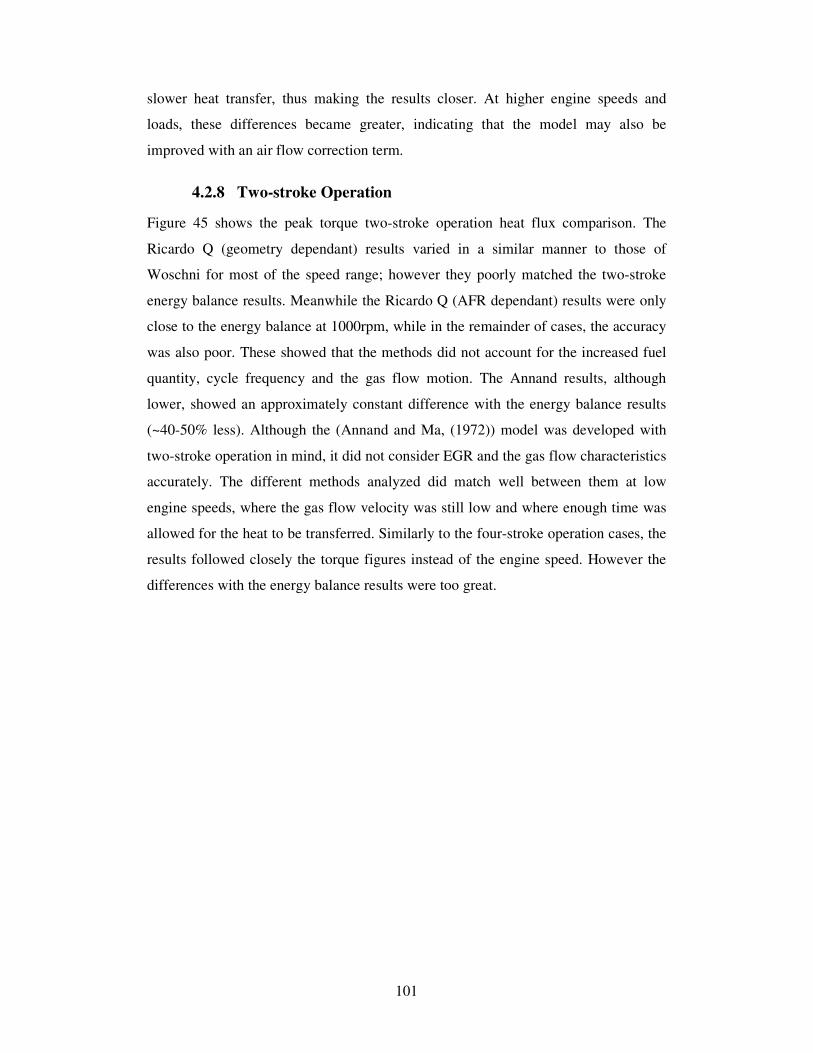
101
slower heat transfer, thus making the results closer. At higher engine speeds and
loads, these differences became greater, indicating that the model may also be
improved with an air flow correction term.
4.2.8 Two-stroke Operation
Figure 45 shows the peak torque two-stroke operation heat flux comparison. The
Ricardo Q (geometry dependant) results varied in a similar manner to those of
Woschni for most of the speed range; however they poorly matched the two-stroke
energy balance results. Meanwhile the Ricardo Q (AFR dependant) results were only
close to the energy balance at 1000rpm, while in the remainder of cases, the accuracy
was also poor. These showed that the methods did not account for the increased fuel
quantity, cycle frequency and the gas flow motion. The Annand results, although
lower, showed an approximately constant difference with the energy balance results
(~40-50% less). Although the (Annand and Ma, (1972)) model was developed with
two-stroke operation in mind, it did not consider EGR and the gas flow characteristics
accurately. The different methods analyzed did match well between them at low
engine speeds, where the gas flow velocity was still low and where enough time was
allowed for the heat to be transferred. Similarly to the four-stroke operation cases, the
results followed closely the torque figures instead of the engine speed. However the
differences with the energy balance results were too great.
102
Figure 45: Variation in two-stroke net heat flux results at peak torque for: 1000 to
2500rpm.
The two-stroke “F_Factor” results showed a linear relationship, similar to that for
four-stroke operation. Figure 45 showed that there was not a linear increase in the
energy balance, with increasing torque and speed. In four-stroke operation the
geometrical (Q) and AFR dependant (Q (AFR)) Ricardo model results did provide
linear results, when considered at different engine speeds ((Q) values at low and (Q
(AFR)) ones at medium to high engine speeds).
The three main parameters that can be varied in the Ricardo model were: gross fuel
flow, G, boost pressure, PB and boost temperature, TB. The differences with the
energy balance ranged from 35% to 77% lower, in case of the geometrically
dependant Ricardo Q, and 6% to 73% lower for the AFR dependant Ricardo Q (AFR).
A variation in the “F_Factor” for both the geometrical and AFR terms would not be
sufficient to overcome the difference.
It was proposed to introduce a correction term for the torque and gas flow. The model
was derived considering an exponential form. This was obtained from the apparent
“Lambda_ECM”, λECM reading plotted in Figure 46 against speed and torque. In
addition, the air flow was corrected by the mean piston speed, Cm, which was aided by
an empirical correction variable, AR (equal to 3.7), which would correct the results
Two-stroke heat flux
1.5E+05
6.5E+05
1.2E+06
1.7E+06
2.2E+06
2.7E+06
3.2E+06
3.7E+06
rpm
Hea
t fl
ux
Q (
W/m
^2
)
0
50
100
150
200
250
300
To
rqu
e (
Nm
)
Woschni
Annand
Ricardo
Ricardo AFR
Energy balance
Torque
1000 1500 2000 2500
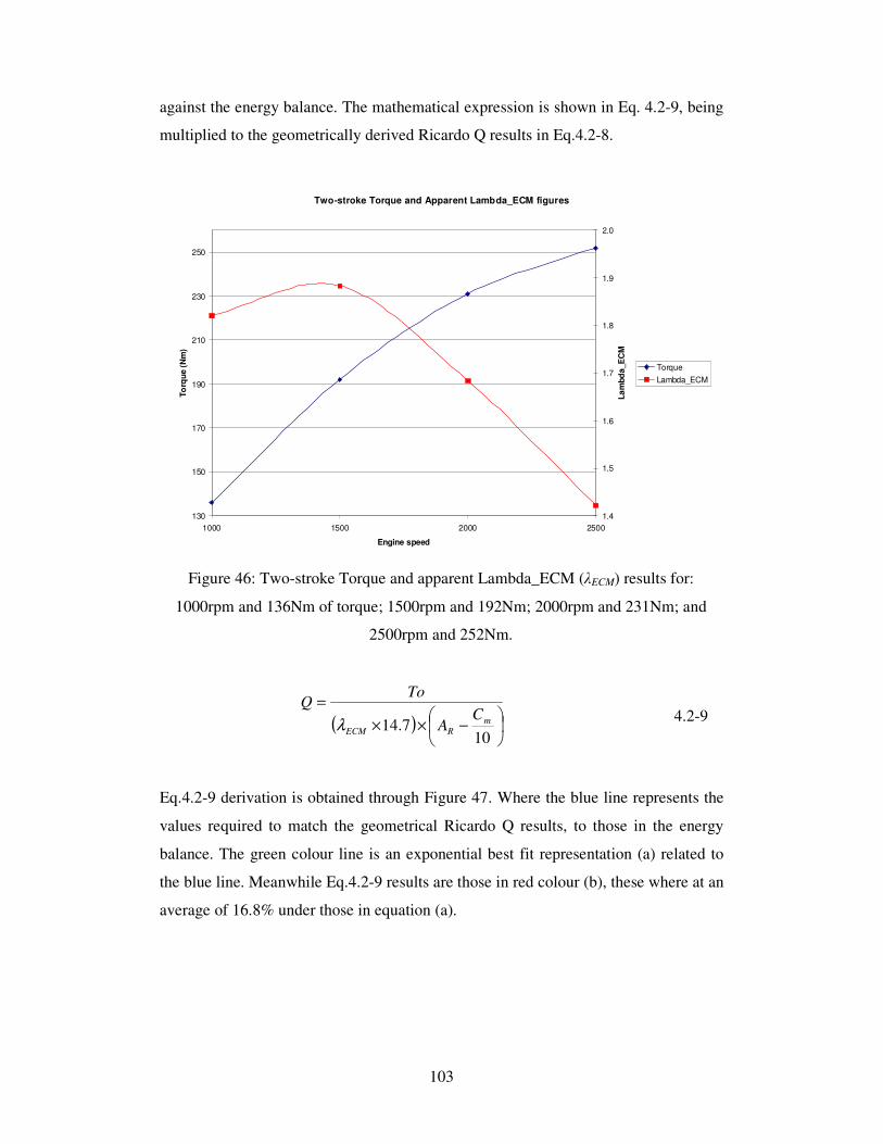
103
against the energy balance. The mathematical expression is shown in Eq. 4.2-9, being
multiplied to the geometrically derived Ricardo Q results in Eq.4.2-8.
Figure 46: Two-stroke Torque and apparent Lambda_ECM (λECM) results for:
1000rpm and 136Nm of torque; 1500rpm and 192Nm; 2000rpm and 231Nm; and
2500rpm and 252Nm.
( )
−××
=
107.14 m
RECM
CA
ToQ
λ
4.2-9
Eq.4.2-9 derivation is obtained through Figure 47. Where the blue line represents the
values required to match the geometrical Ricardo Q results, to those in the energy
balance. The green colour line is an exponential best fit representation (a) related to
the blue line. Meanwhile Eq.4.2-9 results are those in red colour (b), these where at an
average of 16.8% under those in equation (a).
Two-stroke Torque and Apparent Lambda_ECM figures
130
150
170
190
210
230
250
1000 1500 2000 2500
Engine speed
To
rqu
e (
Nm
)
1.4
1.5
1.6
1.7
1.8
1.9
2.0
La
mb
da
_E
CM
Torque
Lambda_ECM

104
Figure 47: Variation in the correction factor for Ricardo geometrical heat flux results
in two-stroke operation for: 1000rpm, 136Nm; 1500rpm, 192Nm; 2000rpm, 231Nm;
and 2500rpm, 252Nm.
A comparison of the two-stroke operation energy balance with the corrected Ricardo
Q results are shown in Figure 48. The percentage error was less than that of the
Annand model range for four-stroke operation. The best comparison is achieved at the
lowest speed and torque conditions.
Variation in correction factor for two-stroke operation
1
1.5
2
2.5
3
3.5
4
4.5
5
5.5
500 1000 1500 2000 2500 3000engine speed
Co
rre
cti
on
fa
cto
r
Ricardo Q to energy
balance results match
Best fit model, equation (a)
Correction factor results,equation (b)
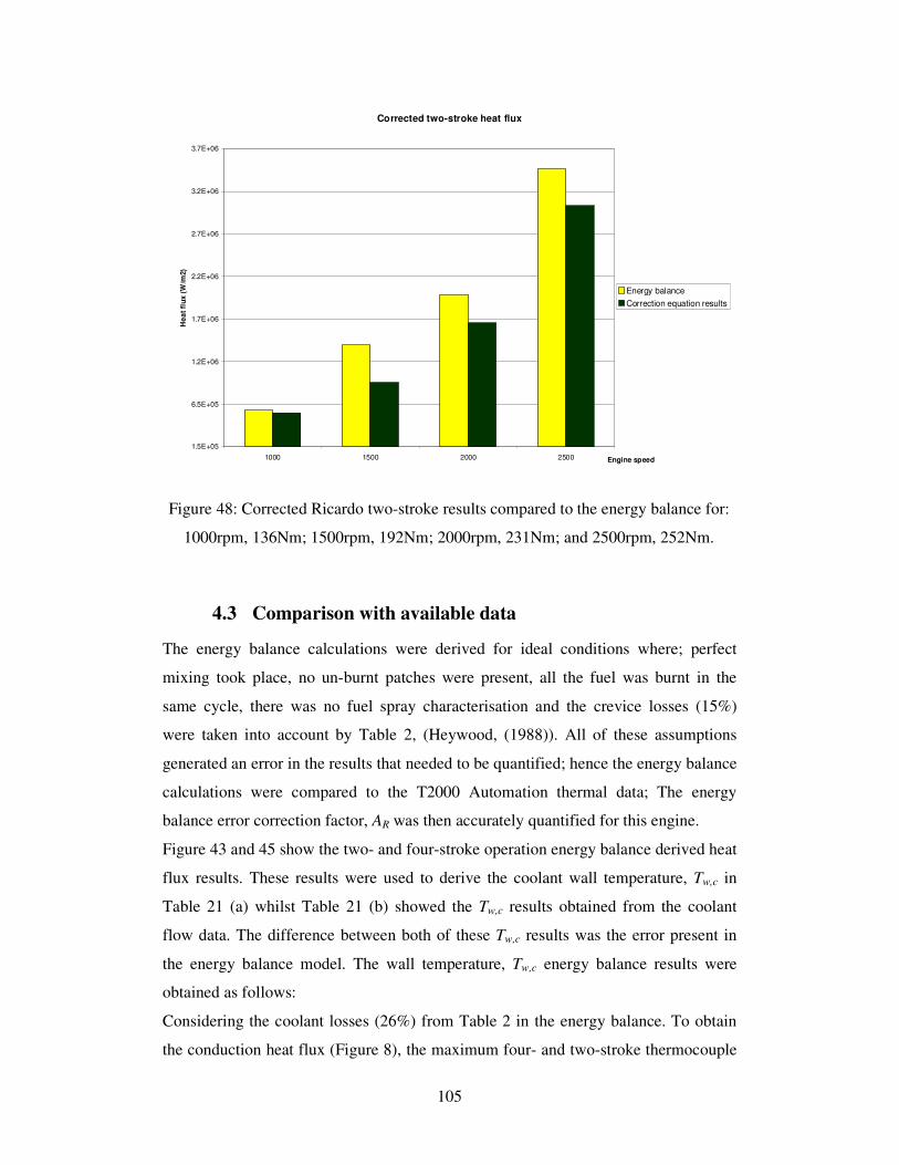
105
Figure 48: Corrected Ricardo two-stroke results compared to the energy balance for:
1000rpm, 136Nm; 1500rpm, 192Nm; 2000rpm, 231Nm; and 2500rpm, 252Nm.
4.3 Comparison with available data
The energy balance calculations were derived for ideal conditions where; perfect
mixing took place, no un-burnt patches were present, all the fuel was burnt in the
same cycle, there was no fuel spray characterisation and the crevice losses (15%)
were taken into account by Table 2, (Heywood, (1988)). All of these assumptions
generated an error in the results that needed to be quantified; hence the energy balance
calculations were compared to the T2000 Automation thermal data; The energy
balance error correction factor, AR was then accurately quantified for this engine.
Figure 43 and 45 show the two- and four-stroke operation energy balance derived heat
flux results. These results were used to derive the coolant wall temperature, Tw,c in
Table 21 (a) whilst Table 21 (b) showed the Tw,c results obtained from the coolant
flow data. The difference between both of these Tw,c results was the error present in
the energy balance model. The wall temperature, Tw,c energy balance results were
obtained as follows:
Considering the coolant losses (26%) from Table 2 in the energy balance. To obtain
the conduction heat flux (Figure 8), the maximum four- and two-stroke thermocouple
Corrected two-stroke heat flux
1.5E+05
6.5E+05
1.2E+06
1.7E+06
2.2E+06
2.7E+06
3.2E+06
3.7E+06
1000 1500 2000 2500 Engine speed
He
at
flu
x (
W/m
2)
Energy balance
Correction equation results
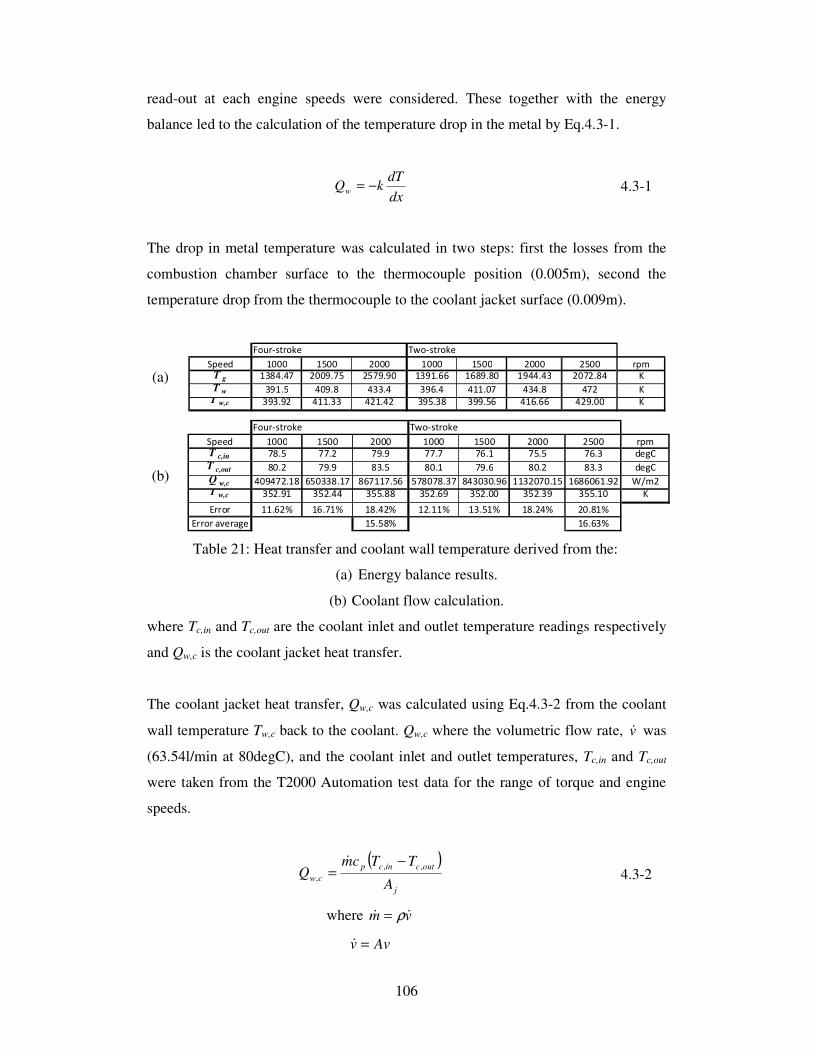
106
read-out at each engine speeds were considered. These together with the energy
balance led to the calculation of the temperature drop in the metal by Eq.4.3-1.
dx
dTkQw −= 4.3-1
The drop in metal temperature was calculated in two steps: first the losses from the
combustion chamber surface to the thermocouple position (0.005m), second the
temperature drop from the thermocouple to the coolant jacket surface (0.009m).
(a)
(b)
Table 21: Heat transfer and coolant wall temperature derived from the:
(a) Energy balance results.
(b) Coolant flow calculation.
where Tc,in and Tc,out are the coolant inlet and outlet temperature readings respectively
and Qw,c is the coolant jacket heat transfer.
The coolant jacket heat transfer, Qw,c was calculated using Eq.4.3-2 from the coolant
wall temperature Tw,c back to the coolant. Qw,c where the volumetric flow rate, v& was
(63.54l/min at 80degC), and the coolant inlet and outlet temperatures, Tc,in and Tc,out
were taken from the T2000 Automation test data for the range of torque and engine
speeds.
( )
j
outcincp
cwA
TTcmQ
,,
,
−=
& 4.3-2
where vm && ρ=
Avv =&
Four-stroke Two-stroke
Speed 1000 1500 2000 1000 1500 2000 2500 rpmT c,in 78.5 77.2 79.9 77.7 76.1 75.5 76.3 degC
T c,out 80.2 79.9 83.5 80.1 79.6 80.2 83.3 degC
Q w,c 409472.18 650338.17 867117.56 578078.37 843030.96 1132070.15 1686061.92 W/m2T w,c 352.91 352.44 355.88 352.69 352.00 352.39 355.10 K
Error 11.62% 16.71% 18.42% 12.11% 13.51% 18.24% 20.81%
Error average 15.58% 16.63%
Four-stroke Two-stroke
Speed 1000 1500 2000 1000 1500 2000 2500 rpmT g 1384.47 2009.75 2579.90 1391.66 1689.80 1944.43 2072.84 K
T w 391.5 409.8 433.4 396.4 411.07 434.8 472 KT w,c 393.92 411.33 421.42 395.38 399.56 416.66 429.00 K
107
where Aj is the area of coolant jacket surface next to the combustion chamber.
The contact area, Aj was shown in Figure 20. However the coolant jacket was
assumed to be a pipe of diameter equal to that of the coolant inlet (0.025m), where Aj
was the total pipe area (0.0177m2). Considering the Reynolds number analogy in
Eq.4.3-3 from (Stone, (1999)), the cooling medium heat transfer coefficient, h was
calculated as 733.69 (W/m2K) using:
4.08.0 PrRe023.0=Nu 4.3-3
where vm && ρ=
12
4
−
=
dvm
πρ&
Newton’s Law of Convection was used to calculate the coolant wall temperature, Tw,c
using Eq.4.3-4 for both four- and two-stroke operation. The comparison is plotted in
Figure 49.
( )ccwht TThQ −= , 4.3-4
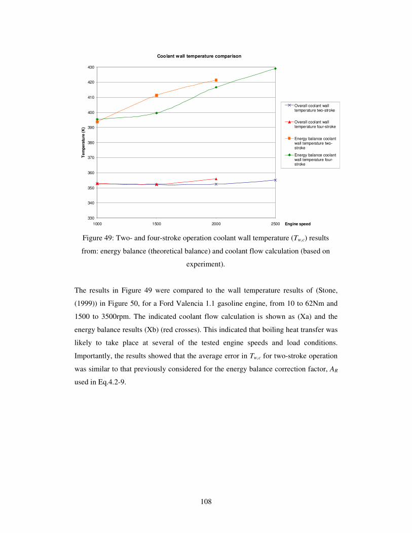
108
Figure 49: Two- and four-stroke operation coolant wall temperature (Tw,c) results
from: energy balance (theoretical balance) and coolant flow calculation (based on
experiment).
The results in Figure 49 were compared to the wall temperature results of (Stone,
(1999)) in Figure 50, for a Ford Valencia 1.1 gasoline engine, from 10 to 62Nm and
1500 to 3500rpm. The indicated coolant flow calculation is shown as (Xa) and the
energy balance results (Xb) (red crosses). This indicated that boiling heat transfer was
likely to take place at several of the tested engine speeds and load conditions.
Importantly, the results showed that the average error in Tw,c for two-stroke operation
was similar to that previously considered for the energy balance correction factor, AR
used in Eq.4.2-9.
Coolant wall temperature comparison
330
340
350
360
370
380
390
400
410
420
430
1000 1500 2000 2500 Engine speed
Te
mp
era
ture
(K
)
Overall coolant walltemperature two-stroke
Overall coolant walltemperature four-stroke
Energy balance coolantwall temperature two-stroke
Energy balance coolantwall temperature four-stroke
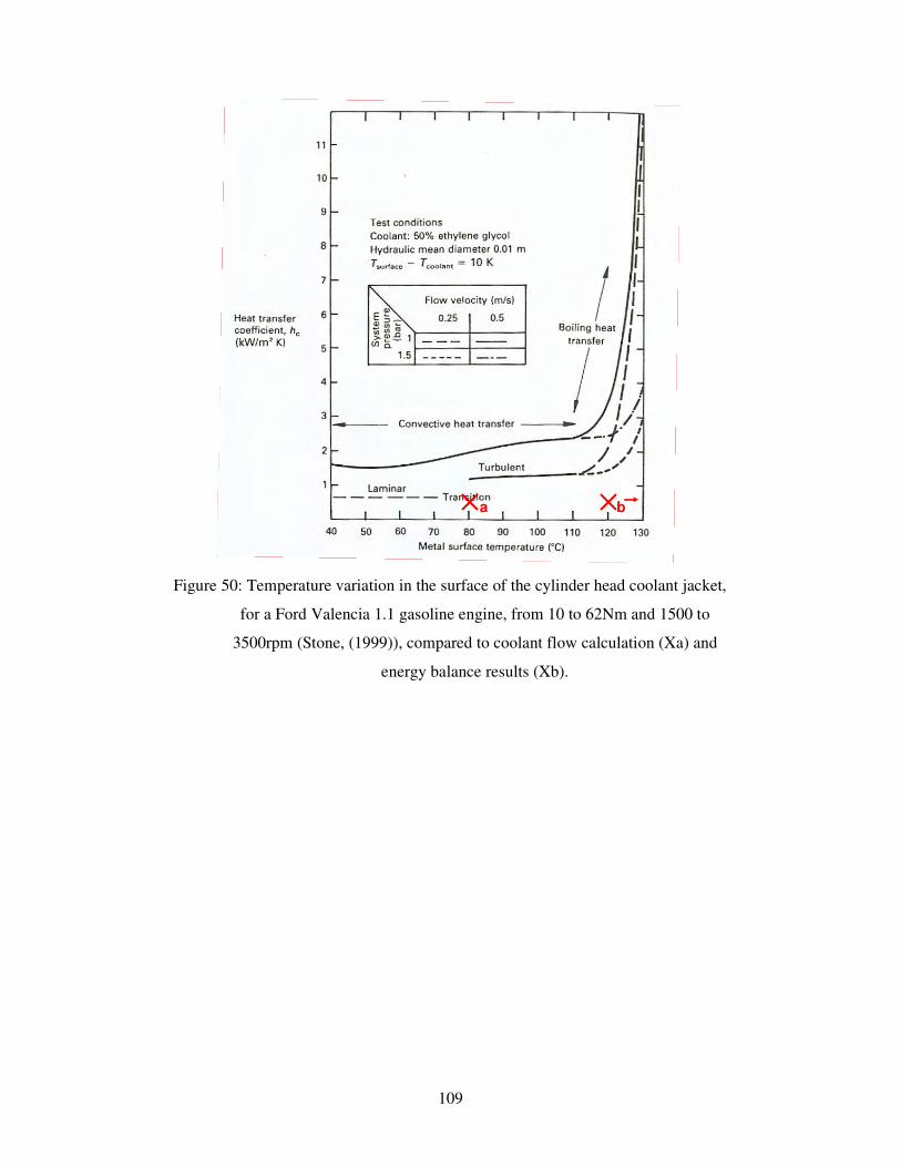
109
Figure 50: Temperature variation in the surface of the cylinder head coolant jacket,
for a Ford Valencia 1.1 gasoline engine, from 10 to 62Nm and 1500 to
3500rpm (Stone, (1999)), compared to coolant flow calculation (Xa) and
energy balance results (Xb).
a ba b

110
5 Conclusions
The characteristics of the thermal performance of an engine that switched between
four- and two-stroke operation was experimentally evaluated. Steady-state operating
engine condition, were considered at maximum torque in the range of 1000 to
2500rpm. The undertaken engine thermal survey was the one recommended by
Ricardo, in which the cooling procedure follows a combination or series flow strategy
and the thermocouples position selection are obtained through company knowledge.
The instrumentation used is well known in the market and have been used in many
similar studies.
The literature review identified some of the most important studies used to correlate
the heat flux and the heat transfer coefficient in IC engines, for both steady-state
operation and with crank angle. The main correlations selected from the literature
were: The (Woschni, (1967)) heat transfer coefficient and (Annand and Ma, (1972))
heat flux correlations. These were implemented and compared to a theoretical energy
balance, at each engine condition. These results were compared to the empirical heat
flux model derived from the Ricardo Q/F expression, which was developed for four-
stroke operation of a Diesel engine. The approach was applied to two-stroke
operation, using the experimental results, with the aim of implementing a correction
factor. The energy balance results were compared to the heat flux results generated
from the coolant temperature into and out of the cylinder head and the coolant flow
rate. A 17% error was obtained between the wall temperatures for both the energy
balance calculation and the coolant flow comparison. This was implemented in a two-
stroke correction factor included in Eq.5.1-1, this considered engine torque, lambda
and mean piston speed terms. This correction factor was supplemented by AR which
would correct the 17% deviation between the energy balance and the coolant flow
comparison calculation. This correction factor is then multiplied to the geometrically
depend Ricardo Q result.
( )
−××
=
107.14 m
RECM
CA
ToQ
λ
5.1-1
111
The energy balance calculation considered the crevice losses and the percentage of
heat flux into the coolant, however no losses to the surroundings and no in cylinder
characteristics were considered such as gas flow motion or fuel spray modelling.
Meanwhile, from the energy balance calculations, it was observed that the EGR in
two-stroke operation acted as a heat sink. The instantaneous gas temperature results in
four-stroke simulation were higher than the two-stroke ones; this was also confirmed
by measurement of the exhaust gas temperature directly. However the higher two-
stroke operating frequency increased the metal temperature over that of the four-
stroke (but not doubled). In terms of the metal temperature results, safe operation was
guaranteed for engine speeds for up to 2500rpm in two-stroke operation, where the
results go over 180degC. At this temperature the oil can be damaged and the
recommended temperature limit for aluminium was exceeded.
112
6 Recommendations for further work
The series of calculations and experiments together with the literature review
highlight the complexity of the problem and how, through different mathematical
models, different researchers have tried to obtain accurate results. In order to obtain
more precise information, the following studies are recommended:
• More complex computer simulations are suggested. This could be an energy
balance that considers the effects of the in-cylinder phenomena such as air
flow, ignition and spray modelling.
• A first approach would be a full engine 1-D flow simulation.
• A second approach would be matching these results with a three dimensional
computer fluid dynamics simulation, incorporating; the heat transfer in the
piston, the cylinder head and cylinder block for a whole engine cycle, while
also taking into account an experimentally validated blow-by model. This
would generate an engine thermal map in which to compare the thermocouple
results from the current engine.
• A third approach would be a finite element analysis study where the thermal
stresses over the combustion chamber are obtained, thus allowing to calculate
the instantaneous local heat flux.
• In addition, a more detailed cooling model may be considered where different
critical areas are taken into account. This would quantify the heat flux in the
combustion chamber volume, allowing correlation of a crank angle dependant
spatially averaged heat transfer coefficient equation for two-stroke poppet
valve engines.
Secondly the EGR effects needs to be fully investigated since this had great effects in
the two-stroke temperature results.
It may also be required to implement time-resolved experimental measurements of the
combustion chamber surface and gas phase temperature. This may be achieved using
thermo-graphic phosphor parts of powders, aided with high-speed camera and or
infra-red detection methods.

113
7 References
ANNAND, W. J. D. (1962) Heat Transfer in the Cylinders of Reciprocating
Internal Combustion Engines. Proc Inst Mech Eng, 177D, 973-990.
ANNAND, W. J. D. & MA, T. H. (1972) Instantaneous Heat Transfer Rates to the
Cylinder Head Surface of a Small Compression-Ignition Engine. Proc Inst
Mech Eng, 185, 976-987.
BOHNE, D., FISCHER, S. & OBEMEIER, E. (1984) Thermal Conductivity, Density,
Viscosity, and Prandtl-Numbers of Ethylene Glycol - Water Mixtures. Ber.
Bunsen-Ges. Phys. Chem., 88, 739-742.
BORMAN, G. & NISHIWAKI, K. (1987) Internal-combustion engine heat transfer.
Prog in En Comb Sc, 13 p.1.
BULATI, T. (1985) Beitrag zur Berechnung des Warmeuberganges, insbesondere in
Langsgespulten, langhubigen Dieselmotoren. (Improved Analysis of the Heat
transfer, Particulary in Uniflow Scavenged, Long-Stroke Diesel Engines.
Motortechnische Zeitschrift, 46.
BYWATER, R. & TIMMINS, R. (1980) AJ6 Engineering. Cheshire, England.
CARDOSA, T. (2009) Por Fuel Injection Strategies for a Lean Burn Gasoline Engine.
Centre for Automotive Engineering. Brighton, University of Brighton.
CECCARINI, D. (2007) Electro Hydraulic Valve integration with 2/4 stroke Engine
Control Algorithms. IN RICARDO.CO (Ed.) Joint IMechE/IET Automotive
Seminar. Ricardo UK Shoreham, Technical Centre.
DENT, J. C. & SULIAMAN, S. J. (1977) Convective and Radiative Heat Transfer in
a High Swirl Direct Injection Diesel Engine. SAE Paper 770407.
EICHELBERG, G. (1939) Some new investigations on old combustion engine
problems. Engineerng, 148, 547-550.
HAN, S. B., CHUNG, Y. J., KWON, Y. J. & LEE, S. (1997) Empirical Formula for
Instantaneous Heat Transfer Coefficient in Spark Ignition Engine. SaE paper
972995.
HEYWOOD, J. B. (1988) Internal Combustion Engine Fundamentals, McGraw Hill.
HOHEMBERG, G. F. (1980) Advanced Approaches for Heat Transfer Calculations.
SAE Paper 790825.
IMABEPPU, S., SHIMONOSONO, H., HIRANO, Y., FUJIGAYA, K. & INOUE, K.
(1993) Development of a Method for Predicting Heat Rejection to the Engine
Coolant. SAE paper 931114.
KOUREMENOS, D. A., RAKOPOULOS, C. D. & HOUNTALAS, D. T. (1988)
Thermodynamic Analysis of a Divided Combustion Chamber Diesel Engine.
VDI. Forschung im Ingenieurwesen, 54, 73-81.
LAWTON, B. (1987) Effect of compression and expansion on instantaneous heat
transfer in reciprocating internal combustion engines. Inst Mech Eng, 201(A3),
175-186.
MILTON, E. B. (1995) Thermodynamics, Combustion and Engines, Kensington,
Australia, Chapman & Hall.
MONAGHAN, M. L. (1972) Thermal Loading In Internal Combustion Engines.
Ricardo and Co, Ltd, Internal paper.
MONAGHAN.M.L. (1972) Thermal Loading In Internal Combustion Engines.
Ricardo and Co, Ltd, Internal paper.
OGURI, T. (1960) On the Coefficient of Heat Transfer between Gases and Cylinder
Walls of the Spark-Ignition Engine. Bull of JSME, 3, 363-369.

114
OSBORNE, R. J., STOKES, J., CECCARINI, D., JACKSON, N., LAKE, T. H.,
JOYCE, M., VISSER, S., MICHE, N., BEGG, S. M., HEIKAL, M. R.,
KALIAN, N., ZHAO, H. & MA, T. (2008) The 2/4SIGHT Project -
Development of a Multi-Cylinder Two-Stroke/Four-Stroke Switching
Gasoline Engine. 384-20085400.
PFLAUM, W. (1963) Heat Transfer in Internal Combustion Engines. La
Termotecnica, Milano, 235-246.
RICARDO, C. (1996) Design and development of engine cooling systems.
DP96/2651.
RICARDO, C. (2006) WAVEv7.
RICARDO, C. (2008) Ricardo Quarterly Review. Ricardo.
SIHLING, K. & WOSCHNI, G. (1979) Experimental Investigations of the
instantaneous Heat Transfer in the Cylinder of a High-Speed Diesel Engine.
SAE Paper 790833.
SIHLING.K. & WOSCHNI.G. (1979) Experimental Investigations of the
instantaneous Heat Transfer in the Cylinder of a High-Speed Diesel Engine.
SAE Paper 790833.
SITKEI, G. (1974) Heat Transfer and Thermal Loading in Internal Combustion
Engines, Akademiai Kiado.
SITKEI.G (1974) Heat Transfer and Thermal Loading in Internal Combustion
Engines, Akademiai Kiado.
STONE, R. (1999) Introduction to Internal Combustion Engines, Macmillan Press
Ltd.
WOSCHNI, G. (1967) A universally applicable equation for the instantaneous heat
transfer coefficient in the internal combustion engine. SAE paper 670931.
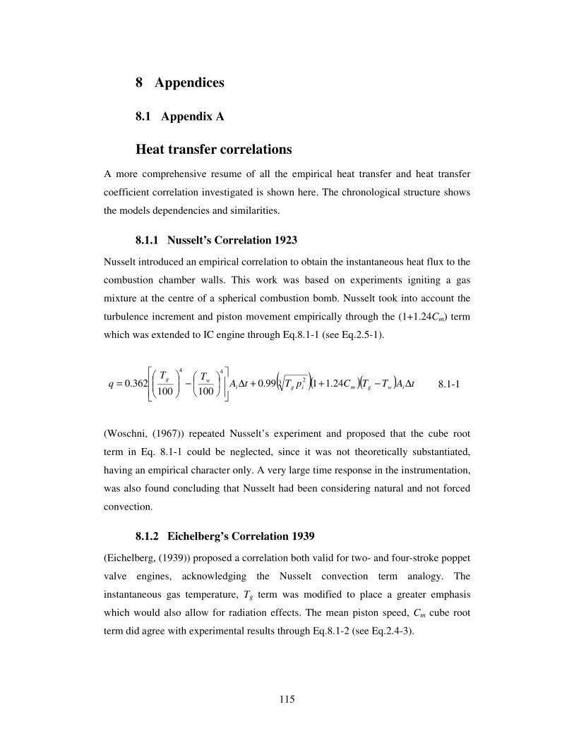
115
8 Appendices
8.1 Appendix A
Heat transfer correlations
A more comprehensive resume of all the empirical heat transfer and heat transfer
coefficient correlation investigated is shown here. The chronological structure shows
the models dependencies and similarities.
8.1.1 Nusselt’s Correlation 1923
Nusselt introduced an empirical correlation to obtain the instantaneous heat flux to the
combustion chamber walls. This work was based on experiments igniting a gas
mixture at the centre of a spherical combustion bomb. Nusselt took into account the
turbulence increment and piston movement empirically through the (1+1.24Cm) term
which was extended to IC engine through Eq.8.1-1 (see Eq.2.5-1).
( )( )( ) tATTCpTtATT
q iwgmigi
wg∆−++∆
−
= 24.1199.0
100100362.0 3 2
44
8.1-1
(Woschni, (1967)) repeated Nusselt’s experiment and proposed that the cube root
term in Eq. 8.1-1 could be neglected, since it was not theoretically substantiated,
having an empirical character only. A very large time response in the instrumentation,
was also found concluding that Nusselt had been considering natural and not forced
convection.
8.1.2 Eichelberg’s Correlation 1939
(Eichelberg, (1939)) proposed a correlation both valid for two- and four-stroke poppet
valve engines, acknowledging the Nusselt convection term analogy. The
instantaneous gas temperature, Tg term was modified to place a greater emphasis
which would also allow for radiation effects. The mean piston speed, Cm cube root
term did agree with experimental results through Eq.8.1-2 (see Eq.2.4-3).
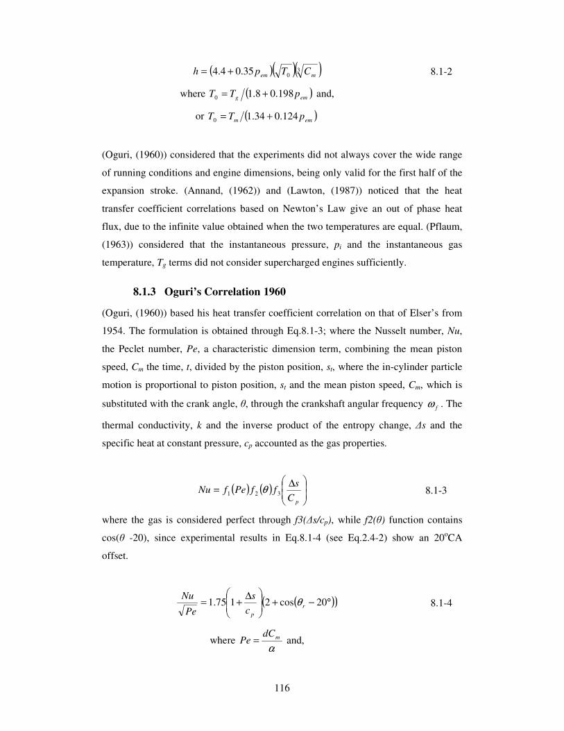
116
( )( )( )3035.04.4 mem CTph += 8.1-2
where ( )emg pTT 198.08.10 += and,
or ( )emm pTT 124.034.10 +=
(Oguri, (1960)) considered that the experiments did not always cover the wide range
of running conditions and engine dimensions, being only valid for the first half of the
expansion stroke. (Annand, (1962)) and (Lawton, (1987)) noticed that the heat
transfer coefficient correlations based on Newton’s Law give an out of phase heat
flux, due to the infinite value obtained when the two temperatures are equal. (Pflaum,
(1963)) considered that the instantaneous pressure, pi and the instantaneous gas
temperature, Tg terms did not consider supercharged engines sufficiently.
8.1.3 Oguri’s Correlation 1960
(Oguri, (1960)) based his heat transfer coefficient correlation on that of Elser’s from
1954. The formulation is obtained through Eq.8.1-3; where the Nusselt number, Nu,
the Peclet number, Pe, a characteristic dimension term, combining the mean piston
speed, Cm the time, t, divided by the piston position, st, where the in-cylinder particle
motion is proportional to piston position, st and the mean piston speed, Cm, which is
substituted with the crank angle, θ, through the crankshaft angular frequency fω . The
thermal conductivity, k and the inverse product of the entropy change, ∆s and the
specific heat at constant pressure, cp accounted as the gas properties.
( ) ( )
∆=
pC
sffPefNu 321 θ 8.1-3
where the gas is considered perfect through f3(∆s/cp), while f2(θ) function contains
cos(θ -20), since experimental results in Eq.8.1-4 (see Eq.2.4-2) show an 20oCA
offset.
( )( )°−+
∆+= 20cos2175.1 r
pc
s
Pe
Nuθ 8.1-4
where α
mdCPe = and,
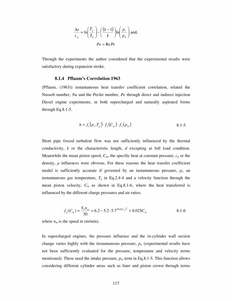
117
( )
−−
=
∆
00
ln1
lnp
p
k
k
T
T
c
s ig
p
and,
PrRe=Pe
Through the experiments the author considered that the experimental results were
satisfactory during expansion stroke.
8.1.4 Pflaum’s Correlation 1963
(Pflaum, (1963)) instantaneous heat transfer coefficient correlation, related the
Nusselt number, Nu and the Peclet number, Pe through direct and indirect injection
Diesel engine experiments, in both supercharged and naturally aspirated forms
through Eq.8.1-5.
( ) ( ) ( )inmgi pfCfTpfh 321 , ⋅⋅= 8.1-5
Short pipe forced turbulent flow was not sufficiently influenced by the thermal
conductivity, k or the characteristic length, d excepting at full load condition.
Meanwhile the mean piston speed, Cm, the specific heat at constant pressure, cp or the
density, ρ influences were obvious. For these reasons the heat transfer coefficient
model is sufficiently accurate if governed by an instantaneous pressure, pi, an
instantaneous gas temperature, Tg in Eq.2.4-4 and a velocity function through the
mean piston velocity, Cm as shown in Eq.8.1-6, where the heat transferred is
influenced by the different charge pressures and air ratios.
( )m
Cmt
m CnS
Cf m 025.07.52.52.630
)(2
01.0
2 +⋅−== 8.1-6
where nm is the speed in (m/min).
In supercharged engines, the pressure influence and the in-cylinder wall section
change varies highly with the instantaneous pressure, pi, (experimental results have
not been sufficiently evaluated for the pressure, temperature and velocity terms
mentioned). These need the intake pressure, pin term in Eq.8.1-5. This function allows
considering different cylinder areas such as liner and piston crown through terms
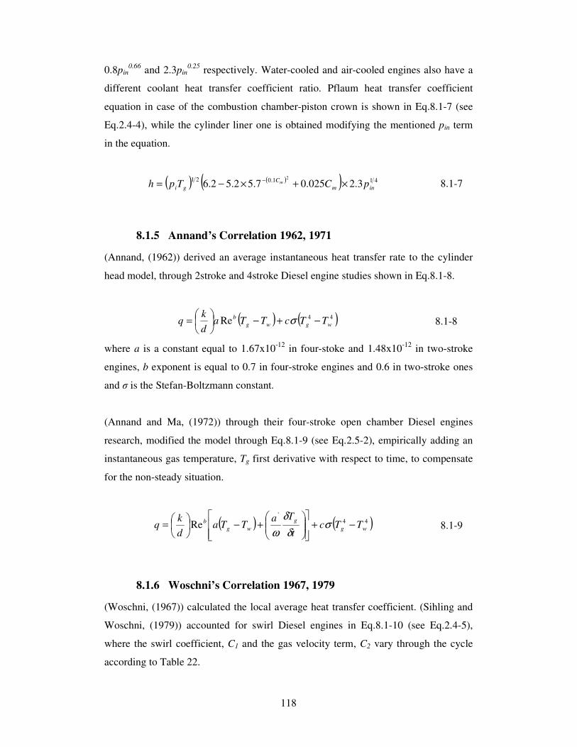
118
0.8pin0.66
and 2.3pin0.25
respectively. Water-cooled and air-cooled engines also have a
different coolant heat transfer coefficient ratio. Pflaum heat transfer coefficient
equation in case of the combustion chamber-piston crown is shown in Eq.8.1-7 (see
Eq.2.4-4), while the cylinder liner one is obtained modifying the mentioned pin term
in the equation.
( ) ( )( ) 411.0213.2025.07.52.52.6
2
inm
C
gi pCTph m ×+×−= − 8.1-7
8.1.5 Annand’s Correlation 1962, 1971
(Annand, (1962)) derived an average instantaneous heat transfer rate to the cylinder
head model, through 2stroke and 4stroke Diesel engine studies shown in Eq.8.1-8.
( ) ( )44Re wgwg
bTTcTTa
d
kq −+−
= σ 8.1-8
where a is a constant equal to 1.67x10⁻¹²
in four-stoke and 1.48x10⁻¹²
in two-stroke
engines, b exponent is equal to 0.7 in four-stroke engines and 0.6 in two-stroke ones
and σ is the Stefan-Boltzmann constant.
(Annand and Ma, (1972)) through their four-stroke open chamber Diesel engines
research, modified the model through Eq.8.1-9 (see Eq.2.5-2), empirically adding an
instantaneous gas temperature, Tg first derivative with respect to time, to compensate
for the non-steady situation.
( ) ( )44'
Re wg
g
wg
bTTc
t
TaTTa
d
kq −+
+−
= σ
δ
δ
ω 8.1-9
8.1.6 Woschni’s Correlation 1967, 1979
(Woschni, (1967)) calculated the local average heat transfer coefficient. (Sihling and
Woschni, (1979)) accounted for swirl Diesel engines in Eq.8.1-10 (see Eq.2.4-5),
where the swirl coefficient, C1 and the gas velocity term, C2 vary through the cycle
according to Table 22.

119
unfired combustion motion
( )m
mi
H
m
m
g
m
i
mpp
Vp
TVCCCTpdh
−+= −−
0
11
121
62.175.01012592.0 8.1-10
Table 22: C1 and C2 term values during different strokes (Sihling.K. and Woschni.G.,
(1979)).
where Cu is the circumferential air speed (m/s).
The Nusselt analogy is considered in this methodology, where m is equal to 0.8 for
turbulent pipe flow situations, while the thermal conductivity, k and the dynamic fluid
viscosity µ are assumed proportional to the instantaneous gas temperature, Tg through
Eq.2.4-9. The mean cylinder gas temperature gT may be calculated through the
equation of state Eq.8.1-11.
Rm
MVpT
a
olHi
g ~= 8.1-11
where nRTPV = and olM
mn =
where Mol is the molecular weight in (mol).
(Annand and Ma, (1972)) considered that the analysis based on the Nusselt analogy
limited the experimental accuracy from 40oCA before TDC to 60
oCA after TDC
during the compression and the expansion stroke respectively.
(Bulati, (1985)) changed the Woschni constant to 1.2592x10⁻²
(W/m2K).
Period No swirl engines Swirl engines Both
Scavenging
Compression
Combustion
Expansion
1C 1C 2C
18.6
28.2
m
u
C
C417.018.6 +
m
u
C
C417.018.6 +
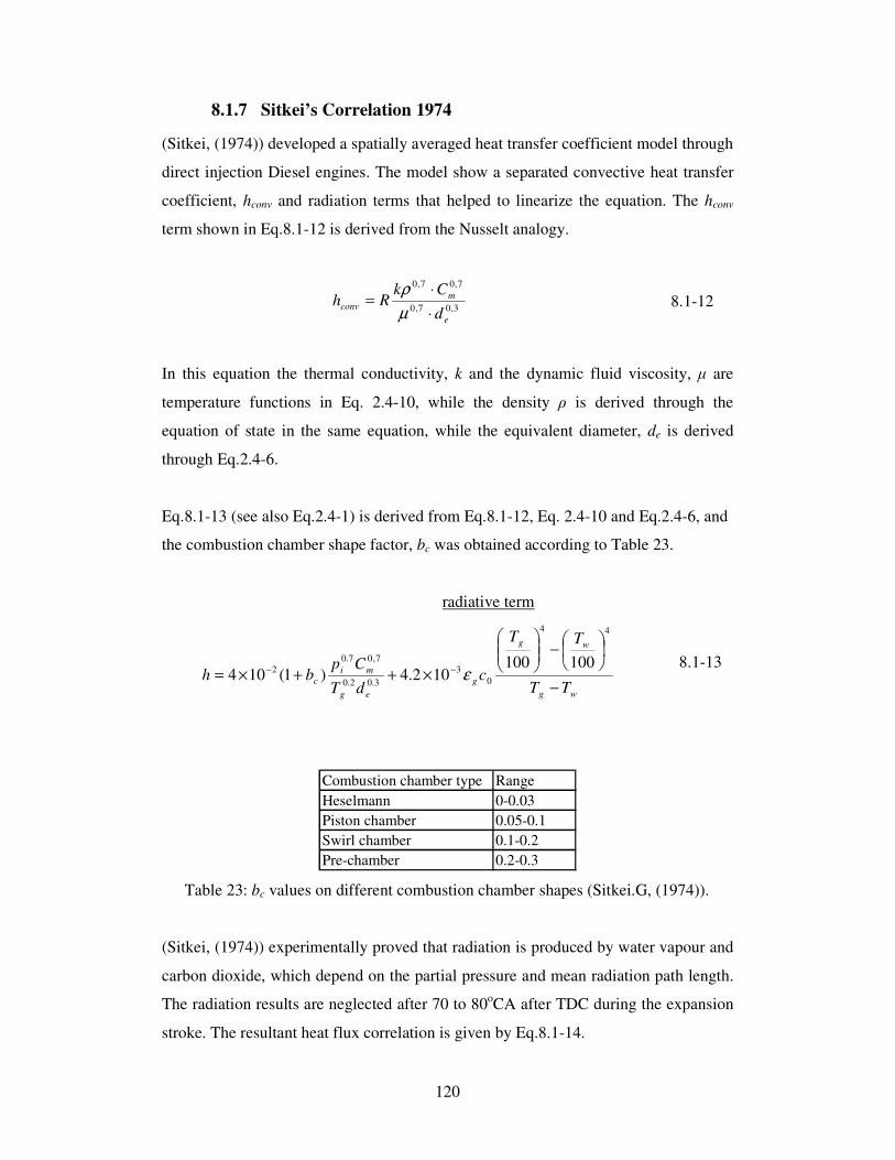
120
8.1.7 Sitkei’s Correlation 1974
(Sitkei, (1974)) developed a spatially averaged heat transfer coefficient model through
direct injection Diesel engines. The model show a separated convective heat transfer
coefficient, hconv and radiation terms that helped to linearize the equation. The hconv
term shown in Eq.8.1-12 is derived from the Nusselt analogy.
3,07,0
7,07,0
e
m
convd
CkRh
⋅
⋅=
µ
ρ 8.1-12
In this equation the thermal conductivity, k and the dynamic fluid viscosity, µ are
temperature functions in Eq. 2.4-10, while the density ρ is derived through the
equation of state in the same equation, while the equivalent diameter, de is derived
through Eq.2.4-6.
Eq.8.1-13 (see also Eq.2.4-1) is derived from Eq.8.1-12, Eq. 2.4-10 and Eq.2.4-6, and
the combustion chamber shape factor, bc was obtained according to Table 23.
radiative term
wg
wg
g
eg
mi
cTT
TT
cdT
Cpbh
−
−
×++×= −−
44
0
3
3.02.0
7,07.0
2100100
102.4)1(104 ε 8.1-13
Table 23: bc values on different combustion chamber shapes (Sitkei.G, (1974)).
(Sitkei, (1974)) experimentally proved that radiation is produced by water vapour and
carbon dioxide, which depend on the partial pressure and mean radiation path length.
The radiation results are neglected after 70 to 80oCA after TDC during the expansion
stroke. The resultant heat flux correlation is given by Eq.8.1-14.
Combustion chamber type Range
Heselmann 0-0.03
Piston chamber 0.05-0.1
Swirl chamber 0.1-0.2
Pre-chamber 0.2-0.3
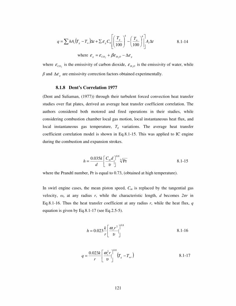
121
( ) tATT
CtTThAq i
wg
gwgi ∆
−
∑+∆−=∑
44
0100100
ε 8.1-14
where gOHCOg εβεεε ∆−+=22
where 2COε is the emissivity of carbon dioxide, OH2
ε is the emissivity of water, while
β and gε∆ are emissivity correction factors obtained experimentally.
8.1.8 Dent’s Correlation 1977
(Dent and Suliaman, (1977)) through their turbulent forced convection heat transfer
studies over flat plates, derived an average heat transfer coefficient correlation. The
authors considered both motored and fired operations in their studies, while
considering combustion chamber local gas motion, local instantaneous heat flux, and
local instantaneous gas temperature, Tg variations. The average heat transfer
coefficient correlation model is shown in Eq.8.1-15. This was applied to IC engine
during the combustion and expansion strokes.
3
8.0
Pr035.0
=
υ
dC
d
kh m 8.1-15
where the Prandtl number, Pr is equal to 0.73, (obtained at high temperature).
In swirl engine cases, the mean piston speed, Cm is replaced by the tangential gas
velocity, ωs at any radius r, while the characteristic length, d becomes 2πr in
Eq.8.1-16. Thus the heat transfer coefficient at any radius r, while the heat flux, q
equation is given by Eq.8.1-17 (see Eq.2.5-5).
8.02
023.0
=
υ
ω r
r
kh s 8.1-16
( )wrg
s TTr
r
kq −
=
8.02
023.0
υ
ω 8.1-17
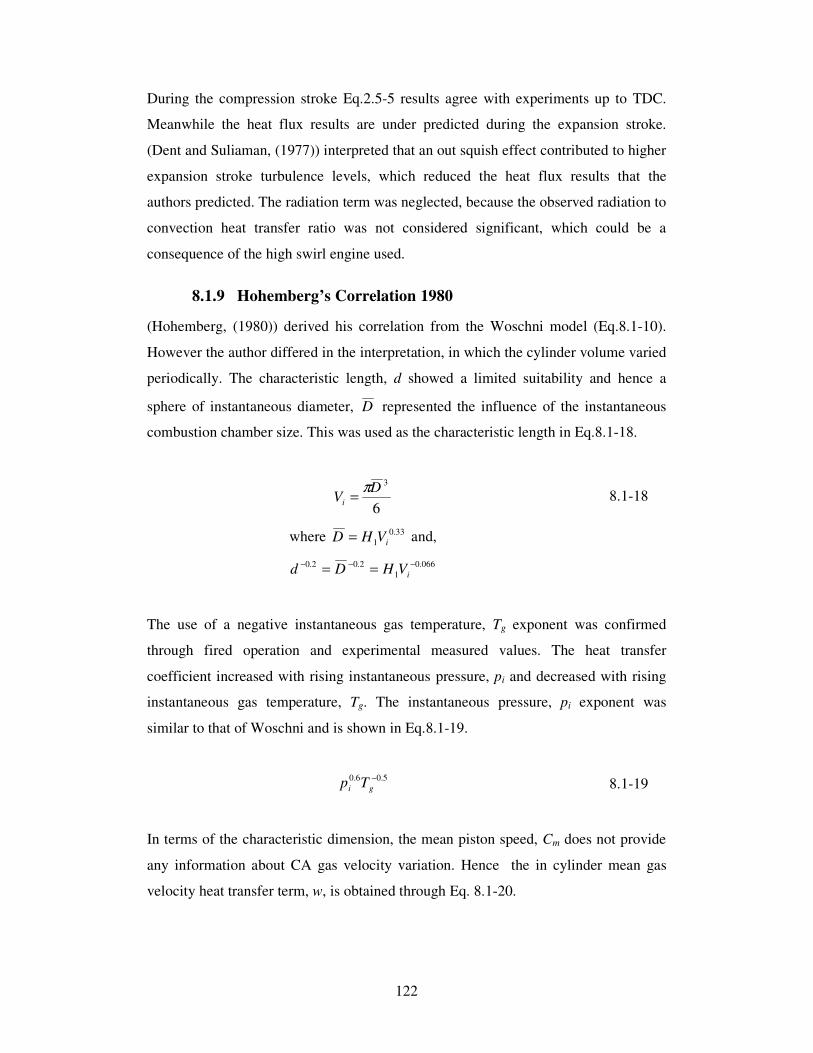
122
During the compression stroke Eq.2.5-5 results agree with experiments up to TDC.
Meanwhile the heat flux results are under predicted during the expansion stroke.
(Dent and Suliaman, (1977)) interpreted that an out squish effect contributed to higher
expansion stroke turbulence levels, which reduced the heat flux results that the
authors predicted. The radiation term was neglected, because the observed radiation to
convection heat transfer ratio was not considered significant, which could be a
consequence of the high swirl engine used.
8.1.9 Hohemberg’s Correlation 1980
(Hohemberg, (1980)) derived his correlation from the Woschni model (Eq.8.1-10).
However the author differed in the interpretation, in which the cylinder volume varied
periodically. The characteristic length, d showed a limited suitability and hence a
sphere of instantaneous diameter, D represented the influence of the instantaneous
combustion chamber size. This was used as the characteristic length in Eq.8.1-18.
6
3D
Vi
π= 8.1-18
where 33.0
1 iVHD = and,
066.0
1
2.02.0 −−− == iVHDd
The use of a negative instantaneous gas temperature, Tg exponent was confirmed
through fired operation and experimental measured values. The heat transfer
coefficient increased with rising instantaneous pressure, pi and decreased with rising
instantaneous gas temperature, Tg. The instantaneous pressure, pi exponent was
similar to that of Woschni and is shown in Eq.8.1-19.
5.06.0 −gi Tp 8.1-19
In terms of the characteristic dimension, the mean piston speed, Cm does not provide
any information about CA gas velocity variation. Hence the in cylinder mean gas
velocity heat transfer term, w, is obtained through Eq. 8.1-20.

123
( ) 8.0
2
1.02.0HCTpw mgi
m += 8.1-20
where the combustion turbulence portion and radiation factor term, H2 is equal to 1.4.
Rearranging Eq.8.1-19, Eq.8.1-18 and Eq. 8.1-20 into the Woschni model from
Eq.2.4-5, Hohemberg model applies in Eq.8.1-21 (see Eq.2.4-7).
( ) 8.0
2
4.08.006.0
1 HCTpVHh mgii += −− 8.1-21
8.1.10 Lawton’s Correlation 1987
(Lawton, (1987)). unsteady heat transfer correlation is based on the (Annand, (1962))
quasi-steady heat flux correlation. The author considered that the heat flux during the
compression stroke was much greater than during the expansion stroke, having a
maximum value at around 8oCA before TDC. From the continuity equation a non
dimensional correlation model was derived:
( )wg
w
TTk
dqaNu
−== 7.0Re 8.1-22
where qw is the wall heat flux (W/m2).
The instantaneous pressure factor, a is equal to 0.28. This compares well to those of
Annand which range between 0.3 and 0.8. The results are underestimated during the
compression stroke; true at TDC and overestimated during the expansion stroke. This
is caused by the assumption of unsteady groups equal to zero. Hence Lawton
considered them in Eq.8.1-23.
−=−
0
0
7.0,
1Re28.0
t
tt
dt
dV
VfNu
γ 8.1-23
where
−=
0
0 ,1
t
tt
dt
dV
Vfr
γε and,
Lr 75.2−=ε
where εr is the error considered between the unsteady and quasi-steady heat fluxes, t
measures time or the CA and 0t is the piston speed.
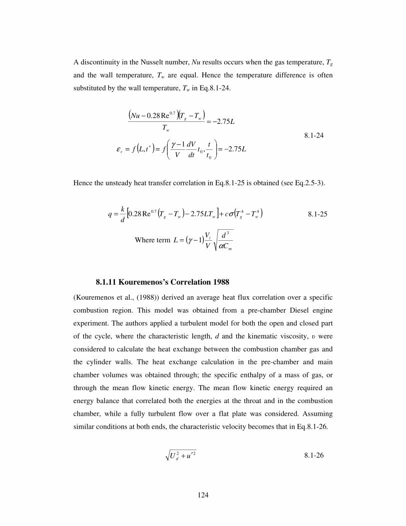
124
A discontinuity in the Nusselt number, Nu results occurs when the gas temperature, Tg
and the wall temperature, Tw are equal. Hence the temperature difference is often
substituted by the wall temperature, Tw in Eq.8.1-24.
( )( )L
T
TTNu
w
wg75.2
Re28.07.0
−=−−
( ) Lt
tt
dt
dV
VftLfr 75.2,
1,
0
0 −=
−== ∗ γ
ε
8.1-24
Hence the unsteady heat transfer correlation in Eq.8.1-25 is obtained (see Eq.2.5-3).
( )[ ] ( )447.0 75.2Re28.0 wgwwg TTcLTTTd
kq −+−−= σ 8.1-25
Where term ( )m
i
C
d
V
VL
αγ
3
1−=
8.1.11 Kouremenos’s Correlation 1988
(Kouremenos et al., (1988)) derived an average heat flux correlation over a specific
combustion region. This model was obtained from a pre-chamber Diesel engine
experiment. The authors applied a turbulent model for both the open and closed part
of the cycle, where the characteristic length, d and the kinematic viscosity, υ were
considered to calculate the heat exchange between the combustion chamber gas and
the cylinder walls. The heat exchange calculation in the pre-chamber and main
chamber volumes was obtained through; the specific enthalpy of a mass of gas, or
through the mean flow kinetic energy. The mean flow kinetic energy required an
energy balance that correlated both the energies at the throat and in the combustion
chamber, while a fully turbulent flow over a flat plate was considered. Assuming
similar conditions at both ends, the characteristic velocity becomes that in Eq.8.1-26.
22 uU d′+ 8.1-26

125
The heat flux was obtained by Eq.2.5-4, where the instantaneous area, Ai was obtained
by Eq.8.1-27 (see Eq.2.1-7) and the radiation heat flux constant, c’ was equal to
3.5x10⁻⁸
.
( ) ( )[ ]44
gwgwi TTcTThAq +′+−= 8.1-27
where 33.0
8.022
33.08.0 Pr037.0
PrRe037.0
′+==
υ
ρ uUd
d
k
d
kh
d
8.1.12 Imabeppu’s Correlation 1993
(Imabeppu et al., (1993)) derived an overall heat transfer coefficient correlation based
on that of Woschni in Eq.2.4-5, where the model is shown in Eq.8.1-28 (see
Eq.2.4-11). It consisted of introducing a heat transfer correction factor, C3 term that
modified the significant amount of heat transfer by the in-cylinder mean gas velocity,
affecting heat transfer, w, where the intake pressure, pin is derived from the equation
of state for gases considering the inducted air to fuel mixture mass.
( ) ( )m
mi
H
m
m
g
m
i
mpp
Vp
TVCCCCTpdh
−++= −−
0
11
1213
62.175.01012592.0 8.1-28
where mint CpIC 035.00008.0003.07.03 +−+=
8.1.13 The Ricardo Empirical Heat Flux Correlation 1996
The Ricardo average heat flux empirical correlation was first introduced by
(Monaghan, (1972)), where the gross fuel flow, G and the inlet air density, Iρ are the
main parameters controlling the heat flux given by.
=
N
AI
AA
M
cA
GFq
ρ
ρ 8.1-29
where F, is the “F Factor”, being a function of combustion chamber type & location
in Figure 51 and AFR (Figure 40).
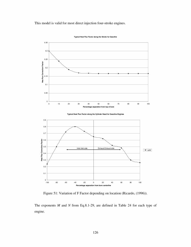
126
This model is valid for most direct injection four-stroke engines.
Figure 51: Variation of F Factor depending on location (Ricardo, (1996)).
The exponents M and N from Eq.8.1-29, are defined in Table 24 for each type of
engine.
Typical Heat Flux Factor along the Cylinder Head for Gasoline Engines
0
0.1
0.2
0.3
0.4
0.5
0.6
0.7
0.8
0.9
-100 -80 -60 -40 -20 0 20 40 60 80 100
Percentage separation from bore centerline
Hea
t F
lux
Co
rre
cti
on
Fa
cto
r
asfsfInlet-Inlet side Exhaust-Exhaust side
Typical Heat Flux Factor along the Stroke for Gasoline
0
0.05
0.1
0.15
0.2
0.25
0.3
0.35
0 10 20 30 40 50 60 70 80 90 100
Percentage separation from top of bore
Hea
Flu
x C
orr
ecti
on
Fac
tor
127
Table 24: M and N exponent values on different engines.
(Ricardo, (1996)) published a modification to that at Eq.8.1-29, allowed correlating
non atmospheric engines through Eq.8.1-30 (see Eq.2.5-6). This included the boost
pressure, PB and boost temperature, TB. The exponent N is fixed value of 0.3, while M
is equal to 0.6 in gasoline and 0.75 in Diesel engines, thus eliminating the combustion
chamber dependency from Table 24.
=
293
B
N
B
A
M
c
T
PA
GFq
ρ 8.1-30
8.1.14 Han’s Correlation 1997
(Han et al., (1997)) introduced an instantaneous heat transfer coefficient (time
varying) correlation, which took into account the instantaneous gas velocity variation,
gv. The authors accepted the Woschni model (Eq.2.4-5). Where the mean piston speed
term, Cm and the in-cylinder time averaged gas velocity were proportional. Hence the
instantaneous gas velocity, gv during the combustion stroke were equal to the sum of
the mean piston speed, Cm and the mixture ignition increase in Cm, besides the gv
change. The heat transfer coefficient was then evaluated through Eq.8.1-31.
( )mm
g
m
i
m wTpdFFNh62.175.01
111
−−=⇔= 8.1-31
where ( )iviviim dpgdgkpNCNw ++= 32
In Eq.8.1-31, the exponent m is equal to 0.75, N1 is the pressure and temperature
related constant equal to 687, N2 is the mean piston speed constant and N3 is an
correction due to the unsteadiness present in the chamber, both N2 and N3 are obtained
comparing the instantaneous gas velocity, gv and the heat release respectively being
0.494 and 0.73.10
-6 respectively, which allows deriving Eq.8.1-32.
Type of engine M N
Comet engines 0.75 0
D.I.with Swirl 0.8 0.3
Quiescent D.I. 0.8 0.3

128
75.0
32
465.075.025.0
1
35.1
++=
−−
δθδθivvi
mgi
dpgdgpNCNTpdNh 8.1-32
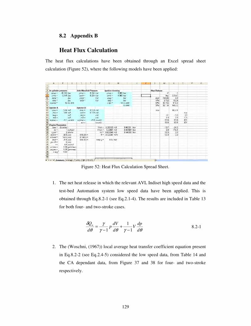
129
8.2 Appendix B
Heat Flux Calculation
The heat flux calculations have been obtained through an Excel spread sheet
calculation (Figure 52), where the following models have been applied:
Figure 52: Heat Flux Calculation Spread Sheet.
1. The net heat release in which the relevant AVL Indiset high speed data and the
test-bed Automation system low speed data have been applied. This is
obtained through Eq.8.2-1 (see Eq.2.1-4). The results are included in Table 13
for both four- and two-stroke cases.
θγθγ
γ
θ
δ
d
dpV
d
dVp
d
Qn
1
1
1 −+
−= 8.2-1
2. The (Woschni, (1967)) local average heat transfer coefficient equation present
in Eq.8.2-2 (see Eq.2.4-5) considered the low speed data, from Table 14 and
the CA dependant data, from Figure 37 and 38 for four- and two-stroke
respectively.
130
( )m
mi
H
m
m
g
m
i
mpp
Vp
TVCCCTpdh
−+= −−
0
11
121
62.175.01012592.0 8.2-2
3. The (Annand and Ma, (1972)) instantaneous heat transfer model in Eq.8.2-3
(see Eq.2.5-2) include the low speed data in Table 16.
( ) ( )44'
Re wg
g
wg
bTTc
t
TaTTa
d
kq −+
+−
= σ
δ
δ
ω 8.2-3
4. The (Ricardo, (1996)) empirical averaged heat transfer model, considered the
low speed data from Table 19, the heat flux “F Factor” dependant on the
AFR from Figure 40 and the geometrical position from Figure 51.
=
293
B
N
B
A
M
c
T
PA
GFq
ρ 8.2-4
5. The energy balance results were compared to the actual in and out coolant
flow rate and the temperature results. This generated a 17% difference
between the wall temperatures from both the energy balance and the coolant
flow calculation. This was then implemented into a correction model that
would be multiplied to the Ricardo Q results (Eq.8.2-4) through Eq.8.2-5 (see
Eq.4.2-9).
( )
−××
107.14 m
RECM
CA
To
λ
8.2-5
The results for both four- and two-stroke operation, applying the models included
above were discussed in Figure 43 and 45 respectively.