Embed Size (px)
Citation preview

© Steven M. Kautz 2009-2011
There are eels in my hovercraft!
An introduction to problem-‐solving and programming using Python
Steve Kautz

[Type text]
Disclaimer
This document is a work in progress. It contains errors and swear words.
© Steven M. Kautz 2009-2011
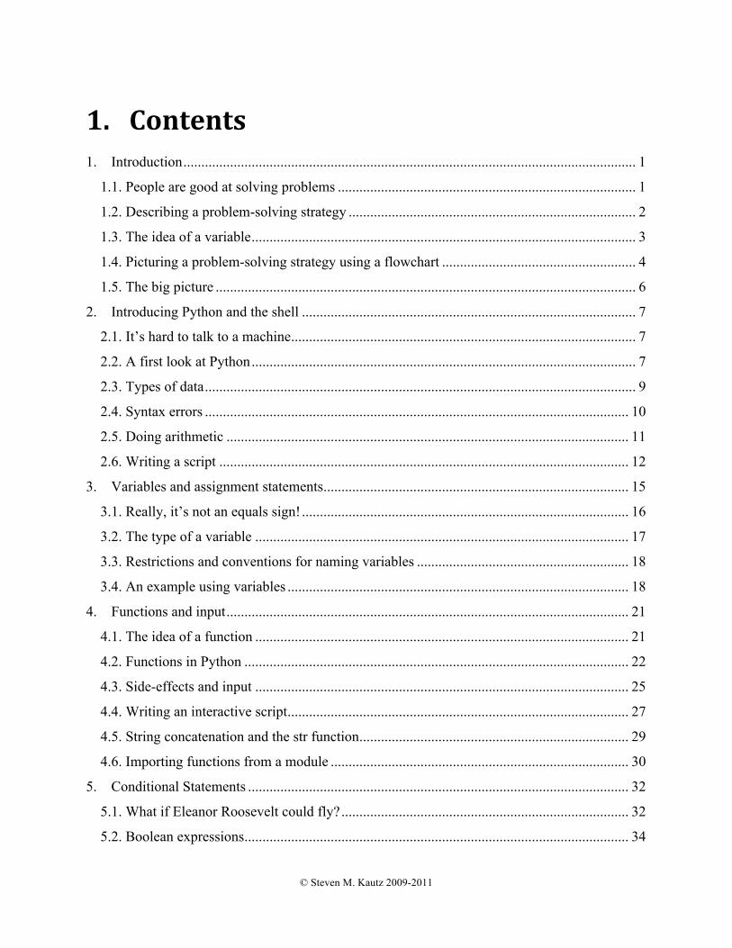
1. Contents 1. Introduction .............................................................................................................................. 1
1.1. People are good at solving problems ................................................................................... 1
1.2. Describing a problem-solving strategy ................................................................................ 2
1.3. The idea of a variable ........................................................................................................... 3
1.4. Picturing a problem-solving strategy using a flowchart ...................................................... 4
1.5. The big picture ..................................................................................................................... 6
2. Introducing Python and the shell ............................................................................................. 7
2.1. It’s hard to talk to a machine ................................................................................................ 7
2.2. A first look at Python ........................................................................................................... 7
2.3. Types of data ........................................................................................................................ 9
2.4. Syntax errors ...................................................................................................................... 10
2.5. Doing arithmetic ................................................................................................................ 11
2.6. Writing a script .................................................................................................................. 12
3. Variables and assignment statements ..................................................................................... 15
3.1. Really, it’s not an equals sign! ........................................................................................... 16
3.2. The type of a variable ........................................................................................................ 17
3.3. Restrictions and conventions for naming variables ........................................................... 18
3.4. An example using variables ............................................................................................... 18
4. Functions and input ................................................................................................................ 21
4.1. The idea of a function ........................................................................................................ 21
4.2. Functions in Python ........................................................................................................... 22
4.3. Side-effects and input ........................................................................................................ 25
4.4. Writing an interactive script ............................................................................................... 27
4.5. String concatenation and the str function ........................................................................... 29
4.6. Importing functions from a module ................................................................................... 30
5. Conditional Statements .......................................................................................................... 32
5.1. What if Eleanor Roosevelt could fly? ................................................................................ 32
5.2. Boolean expressions ........................................................................................................... 34

[Type text]
5.3. Conditional statements ....................................................................................................... 35
5.4. A problem-solving exercise ............................................................................................... 37
6. Nested conditionals ................................................................................................................ 41
6.1. Nested conditionals ............................................................................................................ 41
6.2. A more complex example .................................................................................................. 43
6.3. The elif keyword ................................................................................................................ 46
6.4. Reading code and understanding flow of control ............................................................... 47
7. Writing our own functions ..................................................................................................... 48
7.1. Function parameters ........................................................................................................... 48
7.2. Two kinds of functions ...................................................................................................... 49
7.3. Be the function gnome! ...................................................................................................... 50
7.4. Modules and importing ...................................................................................................... 53
7.5. Local variables ................................................................................................................... 55
8. Value-returning functions ...................................................................................................... 57
8.1. Value-returning functions .................................................................................................. 57
8.2. The special value None ...................................................................................................... 58
8.3. Examples ............................................................................................................................ 59
8.4. Two kinds of functions, and how we use them .................................................................. 61
9. Boolean operators and more about the return statement ................................................... 64
9.1. You will meet a tall and dark or not ugly and rich stranger .............................................. 64
9.2. More about the return statement and flow of control ........................................................ 69
10. Unit testing and incremental development .......................................................................... 73
10.1. An example, and an introduction to unit testing .............................................................. 73
10.2. Another example ............................................................................................................. 80
11. Bugs! .................................................................................................................................... 84
11.1. Finding syntax errors ....................................................................................................... 84
11.2. Runtime errors ................................................................................................................. 87
11.3. Logic errors ...................................................................................................................... 89
11.4. Debugging with multiple modules ................................................................................... 90
12. Binary numbers and data encoding ...................................................................................... 94
12.1. Binary numbers ................................................................................................................ 94
© Steven M. Kautz 2009-2011
12.2. Encoding text ................................................................................................................... 97
12.3. Comparing strings ............................................................................................................ 99
12.4. Other types of data ........................................................................................................... 99
13. Strings and substrings ........................................................................................................ 101
13.1. The bracket notation ...................................................................................................... 101
13.2. Substrings ....................................................................................................................... 102
13.3. Other kinds of sequences ............................................................................................... 104
14. String operations ................................................................................................................ 107
14.1. String methods ............................................................................................................... 107
14.2. Summary of string methods ........................................................................................... 109
14.3. Chaining methods .......................................................................................................... 110
14.4. An example using the find() method ........................................................................ 111
14.5. Format strings ................................................................................................................ 112
15. For-loops ............................................................................................................................ 114
15.1. Water the plants ............................................................................................................. 114
15.2. Number ranges ............................................................................................................... 118
16. For-loop examples ............................................................................................................. 120
16.1. The increment operator “+=” ......................................................................................... 120
16.2. Examples using for-loops .............................................................................................. 121
Example: sum of the elements in a list ............................................................................... 121
Example: counting things in a list ....................................................................................... 122
Example: extracting numbers from a string ........................................................................ 122
Example: maximum value in a list ...................................................................................... 123
16.3. Tracing execution of a loop ........................................................................................... 124
Example: determining whether a value is in a list .............................................................. 124
16.4. Using multiple return statements ................................................................................... 126
Example: determining whether a number is prime ............................................................. 127
16.5. Tables and nested loops ................................................................................................. 127
Example: a table of square roots ......................................................................................... 127
Example: a multiplication table .......................................................................................... 129
17. While-loops ........................................................................................................................ 133
[Type text]
17.1. Beat until smooth ........................................................................................................... 133
17.2. Examples of while-loops ................................................................................................ 137
17.3. Designing a while-loop .................................................................................................. 139
17.4. Example: an interactive game ........................................................................................ 139
18. Examples using while-loops .............................................................................................. 144
18.1. Example: the game of craps ........................................................................................... 144
18.2. Example: a loan table ..................................................................................................... 147
19. Reading text files ............................................................................................................... 152
19.1. Opening and reading a file ............................................................................................. 152
19.2. More examples ............................................................................................................... 155
19.3. Files with numbers ......................................................................................................... 156
19.4. CSV files ........................................................................................................................ 158
19.5. Reading a file with the readlines() function ......................................................... 160
20. Writing text files ................................................................................................................ 162
20.1. Opening a file in write mode ......................................................................................... 162
20.2. Errors .............................................................................................................................. 163
20.3. File processing ............................................................................................................... 165
20.4. A more realistic example ............................................................................................... 166
21. File paths and command shells .......................................................................................... 172
21.1. The path to a file ............................................................................................................ 172
21.2. The working directory and some basic commands ........................................................ 174
21.3. Relative and absolute paths ............................................................................................ 181
21.4. Changing to a different device ....................................................................................... 185
21.5. Running a Python script ................................................................................................. 187
21.6. Command-line arguments .............................................................................................. 194
21.7. Where to go next ............................................................................................................ 195

There are eels in my hovercraft! 1
© Steven M. Kautz 2009-2011
1. Introduction This is a course in problem-solving using a computer. Writing down a set of steps or instructions to make a computer perform some task for you is called programming. We’ll see that there are two parts to this process. Given a problem to solve, we have to
1) figure out what the steps are in solving the problem, and then 2) write them down in such a way that a computer can interpret and carry them out.
You might be concerned about the second part. How do you talk to a computer? But that turns out to be relatively easy. We just need a programming language that our computer can interpret. In this course, we will be using a language called Python. Python is a good choice because it is very simple to start using. (However, keep in mind that this is not an in-depth course in Python; we will really only be using a small fraction of the features of the language.) We will soon discover that the first part – that is, figuring out exactly what steps are involved in solving a problem – is actually much harder than writing instructions in a programming language. Here we will need a pencil and paper and some clear thinking.
1.1. People are good at solving problems
It isn’t that solving problems is difficult. In fact, it is precisely the opposite: people are so good at solving problems, most of the time we’re not aware of how we’re doing it! For example, think about some of the things you do every day that involve some kind of problem-solving strategy: Making a peanut butter and jelly sandwich Finding a parking spot Arranging a time for three friends to meet Getting a good deal on a phone Now, suppose you had to spell out all the steps and little decisions you had to make in order to do one of these tasks. For example, what’s really involved in making a peanut-butter-and-jelly sandwich? Is there bread? Check if the bread is moldy. Find the peanut butter. Remove the lid. If the jar is empty, find another jar. Remove the lid and then the seal from the jar. Find a knife. If there are no knives in the drawer, get a dirty one from the sink and wash it. Use the knife to spread peanut butter on one piece of bread.

2 Introduction
© Steven M. Kautz 2009-2011
And so on. Programming a computer is a bit like this. You really have to spell out every step of the process, because computers can only perform very simple steps.
1.2. Describing a problem-‐solving strategy
Of course, without some fancy robotic arms we certainly aren’t going to program a computer to make sandwiches for us. But here’s a much more straightforward example we can think about. Suppose you have a list of numbers, like this for example: 43 17 85 32 86 79 18 What’s the biggest number in the list? Pretty easy, right? You can just spot the biggest one without even thinking. But what if you had a longer list, maybe like this: 47 26 20 4 60 70 8 24 33 58 20 83 53 95 37 67 85 93 83 49 79 83 61 79 48 28 97 77 89 45 43 41 44 47 31 71 52 22 62 2 82 92 50 1 58 5 26 64 87 82 18 45 11 31 35 59 78 96 91 14 3 65 14 15 94 4 31 41 16 11 43 9 87 1 94 80 2 24 5 21 60 10 97 80 69 61 65 16 89 17 68 77 3 36 50 48 81 6 Well, you might have to be a bit more systematic. Go ahead and find the biggest number, and then ask yourself how you did it. Most of us end up doing something like this:
1. Look at the first number, and remember it (that’s our maximum so far)
2. Read through the rows from left to right
3. If we’ve run out of numbers, then we’re done.
4. Otherwise, look at the next number and compare it to the maximum we remembered
5. If the new number is bigger, then remember that one instead
6. Go back to step 3
The sequence of instructions above gives us a strategy, also called an algorithm, for solving the problem of finding the biggest number in a list. It is a bit more wordy than just saying “find the biggest number in the list”. But that’s how it works: you have to literally write down every step.

There are eels in my hovercraft! 3
© Steven M. Kautz 2009-2011
How do you know when the steps are clear enough? One way to think about how a computer works is that it’s like talking to a kid, say, a reasonably bright fourth-grader. She can read and do fractions and follow directions, but she doesn’t necessarily have any life experience and doesn’t have the “big picture” of what you are trying to accomplish. If you can write down your instructions clearly enough so that a reasonably bright fourth-grader can carry them out, then chances are you’ll be able to program them for a computer too.
1.3. The idea of a variable
One thing to think about here is: what does it mean to “remember” a value, as in step 4 of our strategy above? In programming we need some way to store values and recall them later. We use variables for this purpose. In programming, a variable is a bit like the variables you’ve seen in math books, for example, if someone writes: x = 42 y = 2x + 1 you would probably agree that y is now 85. That is, in the second line you recognize that x still has the value 42. There’s just one important difference between variables in math books and
A reasonably bright 4th-‐grader
Pocket calculator
Clipboard

4 Introduction
© Steven M. Kautz 2009-2011
variables in programming. In programming, the value of a variable can change as the steps are executed. A variable works just like the “memory” key on a pocket calculator. One way to think of a variable is that it is like a page on the clipboard our fourth-grader is holding. She can write down a number, and look it up later, but she can also erase it and write a new number if you ask her to.
1.4. Picturing a problem-‐solving strategy using a flowchart
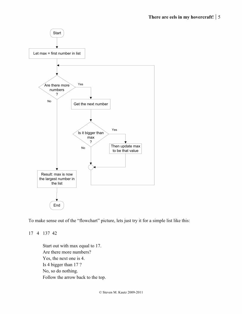
We described our strategy for finding the biggest number as a sequence of written instructions. There is a pictorial way to describe the strategy that will be useful to us, called a flowchart. Sometimes a flowchart is more clear than a sequence of written instructions. You can trace through the steps by following the arrows with your finger. In the flowchart, we’re assuming we have a variable called “max” in which we always store the largest value we’ve seen so far. Each time we find a larger value, we have to update the variable “max.”
There are eels in my hovercraft! 5
© Steven M. Kautz 2009-2011
Are there more numbers
?
No
Yes
Get the next number
Let max = first number in list
Then update max to be that value
Result: max is now the largest number in
the list
Is it bigger than max
?
Yes
No
Start
End
To make sense out of the “flowchart” picture, lets just try it for a simple list like this: 17 4 137 42
Start out with max equal to 17. Are there more numbers? Yes, the next one is 4. Is 4 bigger than 17 ? No, so do nothing. Follow the arrow back to the top.

6 Introduction
© Steven M. Kautz 2009-2011
Are there more numbers? Yes, the next one is 137. Is 137 bigger than 17 ? Yes, so change the value of max to 137 Follow the arrow back to the top. Are there more numbers? Yes, the next one is 42. Is 42 bigger than 137 ? No, so do nothing. Follow the arrow back to the top. Are there more numbers? No, so the result is the value of max, or 137.
1.5. The big picture
Before we break for today let’s take a step back and look at the big picture. What are the ingredients that went into the strategy we described above? Here’s what we needed to be able to do:
• store a value so we can remember it later
• do basic arithmetic (like comparing two numbers)
• check a condition and do something or not, depending on whether the condition is true
• repeat some action, continuing as long as some condition is true
• get input or produce output (in order to read the list and report the result)
The surprising thing is that those five ingredients are enough to any computation. In fact, that is all that any computer ever does! So you can see that the difficulty is programming a computer isn’t that computers are “smart” or “complicated”. The difficulty is that they’re so incredibly stupid that we have spell everything out in detail! The challenge in learning to program is that we have to take our wonderful human problem-solving skills and slow ourselves down enough to analyze how we’re solving a problem, so we can describe the process in simple steps. We have not talked about the second part of the problem-solving process: how to write down the problem-solving strategy so that a computer can do it for us. That’s coming next!

There are eels in my hovercraft! 7
© Steven M. Kautz 2009-2011
2. Introducing Python and the shell In the last unit we brought up the idea that using a computer to solve a problem really has two aspects:
1) figuring out what the steps are in solving the problem, and then 2) writing them down in such a way that a computer can interpret and carry them out.
Last time, as an example of the first aspect, we used the problem of finding the largest number in a list. Remember that we came up with a strategy for solving the problem, and wrote down the steps of the strategy as a sequence of instructions to follow. We also represented the same strategy as a picture called a flowchart. We also made the observation that human beings are really good at solving problems – so good, in fact, that it is sometimes hard for us to slow down and analyze how we’re solving the problem. Today we want to look at the second aspect, and start learning how to write down the steps of a problem-solving strategy so that a computer can execute them.
2.1. It’s hard to talk to a machine
It turns out that human beings are also really, really good at language and communication. You can say all kinds of completely ambiguous things, you can use double meanings, puns, sarcasm, and allusions, and other people will usually know what you’re talking about. For example, “Hey, bring me that thing on the table.” “Life is like a box of chocolates.” “The spirit is willing, but the flesh is weak.” “Your teeth are like stars; they come out at night.” “Let’s play horse. I’ll be the front end, and you can be yourself.” “Why no, that dress doesn’t make you look fat at all.” You cn mespell wrods and use the wroong punctuition and. pepole wil sitll be abel to reed. you're writing withoot any porbelm. But when you’re talking to a computer, it is just the opposite. With a computer you have to use a programming language with very precise structure. You have to get every detail of the grammar and punctuation and spelling just right, and you can’t have any ambiguity at all. Have we mentioned before that computers are really dense?
2.2. A first look at Python

8 Introducing Python and the shell
© Steven M. Kautz 2009-2011
Like most computer languages, Python has the following ingredients:
keywords (such as the print keyword used below) operators (such as +, *, <, etc .) literal values (such as 42, 3.14, “Hello”) identifiers (such as variables and function names) syntax rules (grammar and punctuation)
Statements you write in Python are not directly executed by your computer’s hardware, rather, they are executed by an application called the Python interpreter. One nice thing about the interpreter is that it comes with an interactive shell, where you can easily experiment with the effects of Python statements, and the values of expressions. There are many ways of starting a Python shell. We will suggest some in the lab exercises. But in all cases, when you start the shell you’ll see the prompt “>>>”. This means the shell is ready for you to type something. Here are some things to try: >>> print 42 + 5 47
Let’s figure out what’s going on here.
• The whole thing, print 42 + 5, is a statement. A statement is an instruction to do something. In this case, the print statement is telling the interpreter that it should display something on the screen.
• 42 + 5 is an expression. An expression represents a value. In this case, the value is the
number 47. Notice that 42 + 5 itself has been formed by composing two simpler expressions, 42 and 5, which are literal values.
• print is a Python keyword
Since we are using the interactive shell, the result of executing the print statement is displayed as soon as we type it. We could also display a string of text, surrounded by double or single quotes.
There are eels in my hovercraft! 9
© Steven M. Kautz 2009-2011
>>> print "Hello" Hello >>> print 'Hello' Hello
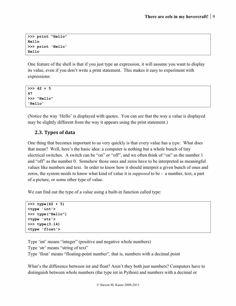
One feature of the shell is that if you just type an expression, it will assume you want to display its value, even if you don’t write a print statement. This makes it easy to experiment with expressions: >>> 42 + 5 47 >>> "Hello" 'Hello'
(Notice the way ‘Hello’ is displayed with quotes. You can see that the way a value is displayed may be slightly different from the way it appears using the print statement.)
2.3. Types of data
One thing that becomes important to us very quickly is that every value has a type. What does that mean? Well, here’s the basic idea: a computer is nothing but a whole bunch of tiny electrical switches. A switch can be “on” or “off”, and we often think of “on” as the number 1 and “off” as the number 0. Somehow those ones and zeros have to be interpreted as meaningful values like numbers and text. In order to know how it should interpret a given bunch of ones and zeros, the system needs to know what kind of value it is supposed to be - a number, text, a part of a picture, or some other type of value. We can find out the type of a value using a built-in function called type: >>> type(42 + 5) <type 'int'> >>> type("Hello") <type 'str'> >>> type(3.14) <type 'float'>
Type ‘int’ means “integer” (positive and negative whole numbers) Type ‘str’ means “string of text” Type ‘float’ means “floating-point number”, that is, numbers with a decimal point What’s the difference between int and float? Aren’t they both just numbers? Computers have to distinguish between whole numbers (the type int in Python) and numbers with a decimal or
10 Introducing Python and the shell
© Steven M. Kautz 2009-2011
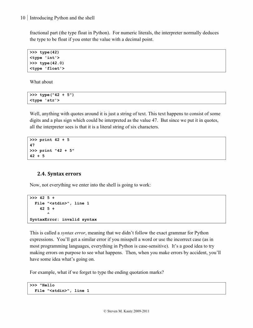
fractional part (the type float in Python). For numeric literals, the interpreter normally deduces the type to be float if you enter the value with a decimal point. >>> type(42) <type 'int'> >>> type(42.0) <type 'float'>
What about >>> type("42 + 5") <type 'str'>
Well, anything with quotes around it is just a string of text. This text happens to consist of some digits and a plus sign which could be interpreted as the value 47. But since we put it in quotes, all the interpreter sees is that it is a literal string of six characters. >>> print 42 + 5 47 >>> print "42 + 5" 42 + 5
2.4. Syntax errors
Now, not everything we enter into the shell is going to work: >>> 42 5 + File "<stdin>", line 1 42 5 + ^ SyntaxError: invalid syntax
This is called a syntax error, meaning that we didn’t follow the exact grammar for Python expressions. You’ll get a similar error if you misspell a word or use the incorrect case (as in most programming languages, everything in Python is case-sensitive). It’s a good idea to try making errors on purpose to see what happens. Then, when you make errors by accident, you’ll have some idea what’s going on. For example, what if we forget to type the ending quotation marks? >>> "Hello File "<stdin>", line 1

There are eels in my hovercraft! 11
© Steven M. Kautz 2009-2011
"Hello ^ SyntaxError: EOL while scanning string literal
What if we misspell the print keyword? >>> rpint "Hello" File "<stdin>", line 1 rpint "Hello" ^ SyntaxError: invalid syntax
What if we accidentally capitalize the keyword?
>>> Print "Hello" File "<stdin>", line 1 Print "Hello" ^ SyntaxError: invalid syntax
As you can see, the error messages don’t always do a very good job of explaining what’s going wrong! Here is a useful tip to remember: when you get an error message in the shell, start reading it at the bottom. Usually the last line in the error message gives you the best clue. Unfortunately, the interpreter doesn’t always “know” what went wrong, it just reports the first place it got stuck trying to interpret what you typed.
2.5. Doing arithmetic
Expressions can be composed from other expressions using the arithmetic operators. These are the ones you are familiar with, except that a star is used for multiplication instead of a dot or “x”. + add - subtract * multiply / divide You can also use parentheses to change the order of operations: >>> (2 * 3) + 4 10 >>> 2 * (3 + 4) 14 >>> 25 / 10 2
12 Introducing Python and the shell
© Steven M. Kautz 2009-2011
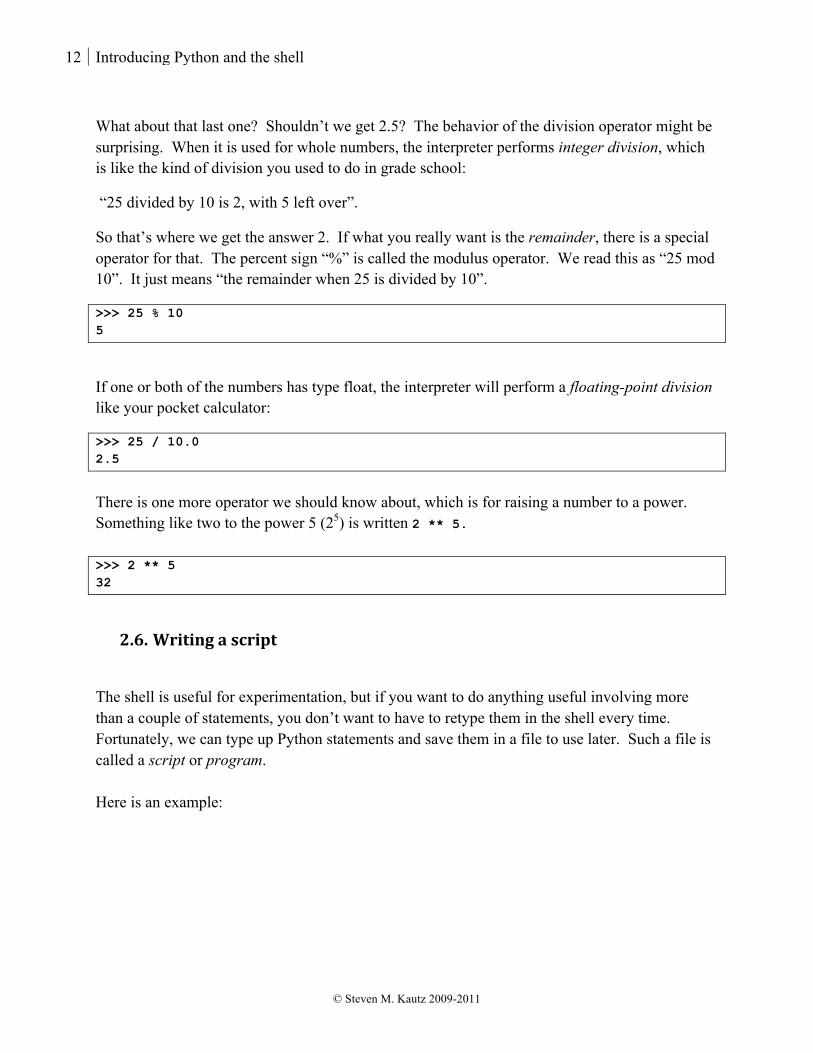
What about that last one? Shouldn’t we get 2.5? The behavior of the division operator might be surprising. When it is used for whole numbers, the interpreter performs integer division, which is like the kind of division you used to do in grade school:
“25 divided by 10 is 2, with 5 left over”.
So that’s where we get the answer 2. If what you really want is the remainder, there is a special operator for that. The percent sign “%” is called the modulus operator. We read this as “25 mod 10”. It just means “the remainder when 25 is divided by 10”.
>>> 25 % 10 5
If one or both of the numbers has type float, the interpreter will perform a floating-point division like your pocket calculator:
>>> 25 / 10.0 2.5
There is one more operator we should know about, which is for raising a number to a power. Something like two to the power 5 (25) is written 2 ** 5. >>> 2 ** 5 32
2.6. Writing a script
The shell is useful for experimentation, but if you want to do anything useful involving more than a couple of statements, you don’t want to have to retype them in the shell every time. Fortunately, we can type up Python statements and save them in a file to use later. Such a file is called a script or program. Here is an example:
There are eels in my hovercraft! 13
© Steven M. Kautz 2009-2011
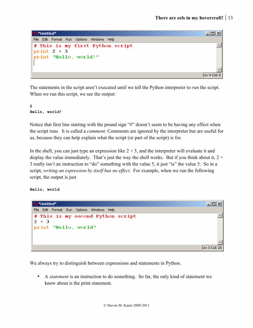
The statements in the script aren’t executed until we tell the Python interpreter to run the script. When we run this script, we see the output: 5 Hello, world!
Notice that first line starting with the pound sign “#” doesn’t seem to be having any effect when the script runs. It is called a comment. Comments are ignored by the interpreter but are useful for us, because they can help explain what the script (or part of the script) is for. In the shell, you can just type an expression like 2 + 3, and the interpreter will evaluate it and display the value immediately. That’s just the way the shell works. But if you think about it, 2 + 3 really isn’t an instruction to “do” something with the value 5, it just “is” the value 5. So in a script, writing an expression by itself has no effect. For example, when we run the following script, the output is just Hello, world
We always try to distinguish between expressions and statements in Python.
• A statement is an instruction to do something. So far, the only kind of statement we know about is the print statement.

14 Introducing Python and the shell
© Steven M. Kautz 2009-2011
• An expression represents a value, such as 2 + 3 or “Hello”.
Try adding an extra space before the print keyword and see what happens. Notice the error message: “unexpected indent”. This reveals one distinctive feature about Python: indentation matters. We will see later how indentation is conveniently used to show the structure of more complicated scripts. There is one other bit of jargon to get used to: programmers refer to anything written in a programming language as “code.”
There are eels in my hovercraft! 15
© Steven M. Kautz 2009-2011
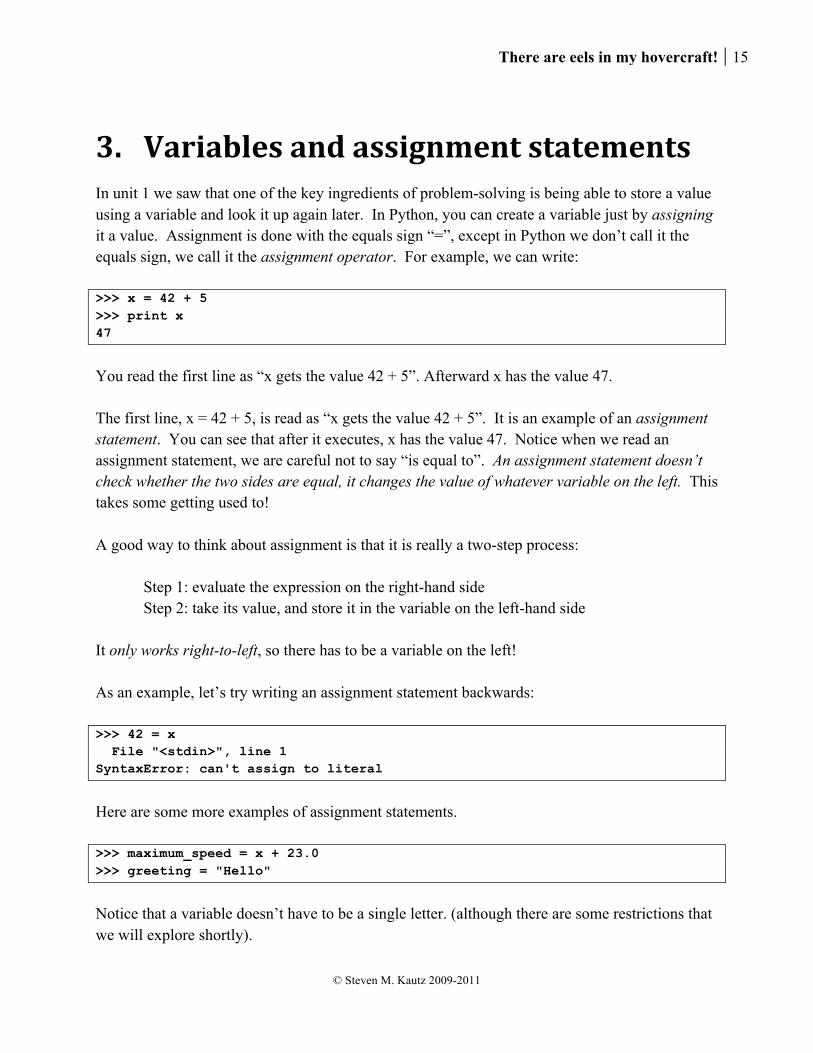
3. Variables and assignment statements In unit 1 we saw that one of the key ingredients of problem-solving is being able to store a value using a variable and look it up again later. In Python, you can create a variable just by assigning it a value. Assignment is done with the equals sign “=”, except in Python we don’t call it the equals sign, we call it the assignment operator. For example, we can write: >>> x = 42 + 5 >>> print x 47
You read the first line as “x gets the value 42 + 5”. Afterward x has the value 47. The first line, x = 42 + 5, is read as “x gets the value 42 + 5”. It is an example of an assignment statement. You can see that after it executes, x has the value 47. Notice when we read an assignment statement, we are careful not to say “is equal to”. An assignment statement doesn’t check whether the two sides are equal, it changes the value of whatever variable on the left. This takes some getting used to! A good way to think about assignment is that it is really a two-step process:
Step 1: evaluate the expression on the right-hand side Step 2: take its value, and store it in the variable on the left-hand side
It only works right-to-left, so there has to be a variable on the left! As an example, let’s try writing an assignment statement backwards: >>> 42 = x File "<stdin>", line 1 SyntaxError: can't assign to literal
Here are some more examples of assignment statements. >>> maximum_speed = x + 23.0 >>> greeting = "Hello"
Notice that a variable doesn’t have to be a single letter. (although there are some restrictions that we will explore shortly).

16 Variables and assignment statements
© Steven M. Kautz 2009-2011
We sometimes draw a “picture” of the effects of an assignment by putting the value of the variable in a box with a label. A picture like this is called a memory map, because in reality the value of each variable is stored in the computer’s memory. After the three assignments above, the memory map would look like this.
3.1. Really, it’s not an equals sign!
With that in mind, let’s look at an example to test our understanding of the two-step process used for an assignment statement. Suppose we write: >>> x = 17 >>> y = x >>> x = 137 >>> print y
Now, after those three statements execute, what is the value of y? Let’s draw a memory map and follow what’s going on. After the assignment x = 17 we have the following (we’ll put a question mark in y’s box to indicate that it hasn’t been defined yet):
47
70.0
“Hello”
x
maximum_speed
greeting
17
?
x
y
There are eels in my hovercraft! 17
© Steven M. Kautz 2009-2011
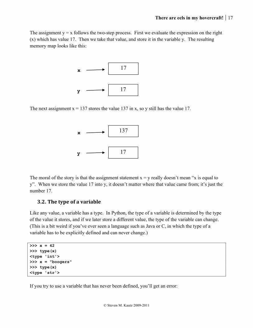
The assignment y = x follows the two-step process. First we evaluate the expression on the right (x) which has value 17. Then we take that value, and store it in the variable y. The resulting memory map looks like this:
The next assignment x = 137 stores the value 137 in x, so y still has the value 17.
The moral of the story is that the assignment statement x = y really doesn’t mean “x is equal to y”. When we store the value 17 into y, it doesn’t matter where that value came from; it’s just the number 17.
3.2. The type of a variable
Like any value, a variable has a type. In Python, the type of a variable is determined by the type of the value it stores, and if we later store a different value, the type of the variable can change. (This is a bit weird if you’ve ever seen a language such as Java or C, in which the type of a variable has to be explicitly defined and can never change.) >>> x = 42 >>> type(x) <type 'int'> >>> x = "boogers" >>> type(x) <type 'str'>
If you try to use a variable that has never been defined, you’ll get an error:
17
17
x
y
137
17
x
y
18 Variables and assignment statements
© Steven M. Kautz 2009-2011
>>> minimum_speed = foo - 7 Traceback (most recent call last): File "<stdin>", line 1, in <module> NameError: name 'foo' is not defined
3.3. Restrictions and conventions for naming variables
We mentioned before that variables don’t have to be single letters, but there are some restrictions. A variable has to be a valid Python identifier, which means that it
• must start with a letter or underscore (not a number),
• must contain only letters, numbers, or underscores (no other spaces or punctuation), and
• can’t be a Python keyword.
There are some conventions too. These are things that the interpreter won’t care about, but that Python programmers find useful.
• Use lowercase letters only
• Use meaningful names for variables that have a particular meaning.
• If there are multiple words, separate them with the underscore character, as in maximum_speed.
3.4. An example using variables
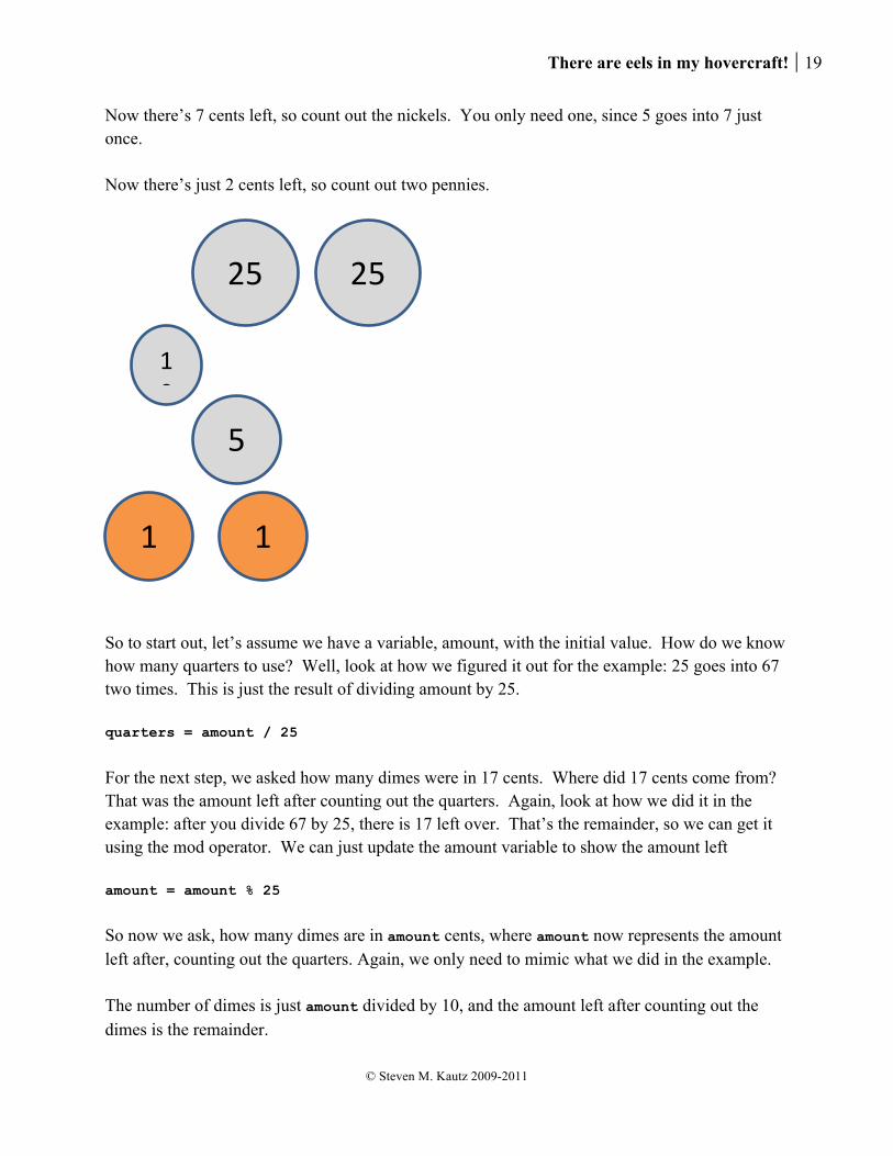
Let’s do an example that uses variables in a simple calculation. Here is the problem we’ll solve: suppose you are given an amount of money in cents, print out how you would make change using quarters, dimes, nickels, and pennies. This is a problem that we have no trouble solving in real life. We just have to analyze how we’re doing it. Let’s start with an example: Suppose you have to make 67 cents in change. Well, we would probably start by counting out two quarters. Why not three quarters? Well, that would be too much, since 25 goes into 67 only two times. Are we done? Not quite, since there’s 17 cents left. So you count out the dimes. You only need one dime, since 10 only goes into 17 once.
There are eels in my hovercraft! 19
© Steven M. Kautz 2009-2011
Now there’s 7 cents left, so count out the nickels. You only need one, since 5 goes into 7 just once. Now there’s just 2 cents left, so count out two pennies.
So to start out, let’s assume we have a variable, amount, with the initial value. How do we know how many quarters to use? Well, look at how we figured it out for the example: 25 goes into 67 two times. This is just the result of dividing amount by 25. quarters = amount / 25
For the next step, we asked how many dimes were in 17 cents. Where did 17 cents come from? That was the amount left after counting out the quarters. Again, look at how we did it in the example: after you divide 67 by 25, there is 17 left over. That’s the remainder, so we can get it using the mod operator. We can just update the amount variable to show the amount left amount = amount % 25
So now we ask, how many dimes are in amount cents, where amount now represents the amount left after, counting out the quarters. Again, we only need to mimic what we did in the example. The number of dimes is just amount divided by 10, and the amount left after counting out the dimes is the remainder.
25 25
10
5
1 1

20 Variables and assignment statements
© Steven M. Kautz 2009-2011
dimes = amount / 10 amount = amount % 10
We do the same thing for the nickels. nickels = amount / 5 amount = amount % 5
And finally the value of the amount variable is just the number of pennies left. The only thing we need to do in order to finish writing the script is to print out the numbers of quarters, dimes, nickels, and pennies. # Script for making change amount = 67 quarters = amount / 25 amount = amount % 25 dimes = amount / 10 amount = amount % 10 nickels = amount / 5 amount = amount % 5 print "Quarters: ", quarters print "Dimes: ", dimes print "Nickels: ", nickels print "Pennies: " , amount
We have the value 67 “hard-coded” in the script above to give an initial value to the amount variable. That’s not very useful! We would have to go in and edit the script every time we want change for a different amount. In the next chapter we’ll learn how to read values that are entered using the keyboard. Before we finish with this example, stop for a moment and look at what we did. The thing to notice is that the general solution to this problem, that works for any amount of change, looks exactly the same as the specific example that gives the answer for 67 cents. That specific example was easy for us to figure out, and doing that first gave us a lot of insight and confidence when we went to write the code. Somewhat ironically, you will find that this is one of the most effective things you can do when you go to start solving a new problem using a computer: get out a pencil and paper, and write out a specific example first!
There are eels in my hovercraft! 21
© Steven M. Kautz 2009-2011
4. Functions and input 4.1. The idea of a function
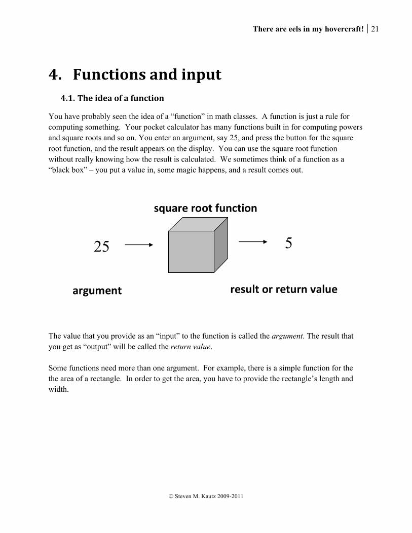
You have probably seen the idea of a “function” in math classes. A function is just a rule for computing something. Your pocket calculator has many functions built in for computing powers and square roots and so on. You enter an argument, say 25, and press the button for the square root function, and the result appears on the display. You can use the square root function without really knowing how the result is calculated. We sometimes think of a function as a “black box” – you put a value in, some magic happens, and a result comes out.
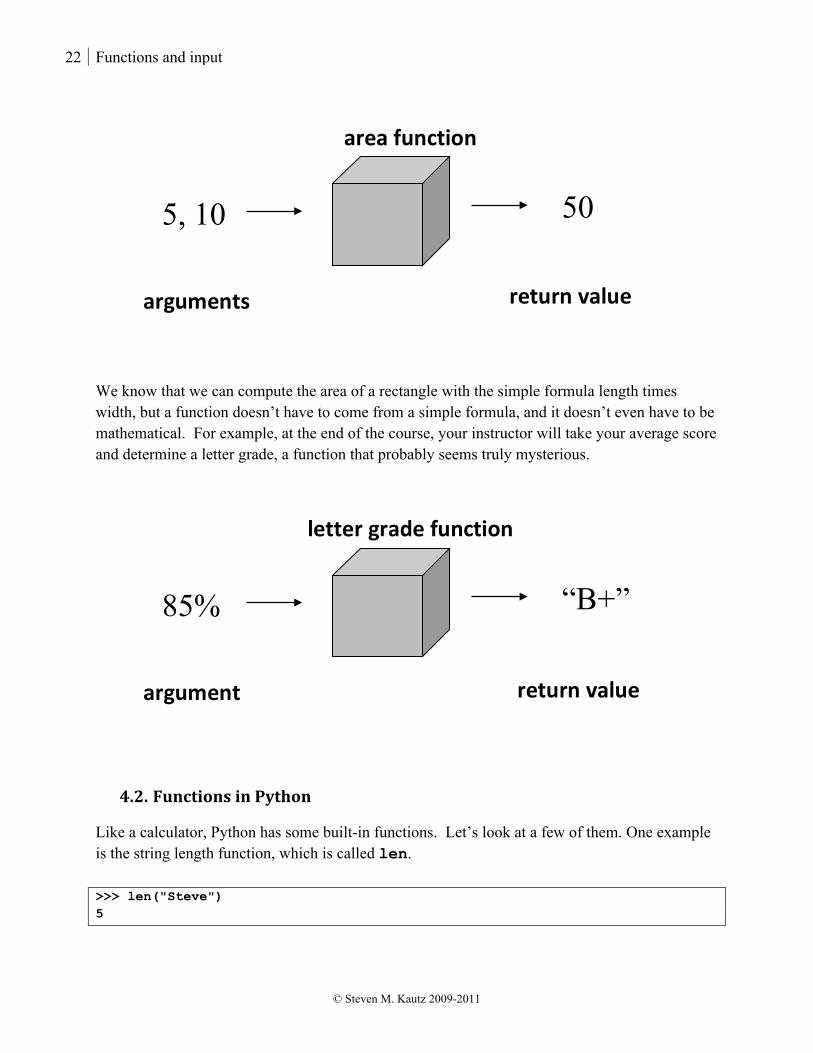
The value that you provide as an “input” to the function is called the argument. The result that you get as “output” will be called the return value. Some functions need more than one argument. For example, there is a simple function for the the area of a rectangle. In order to get the area, you have to provide the rectangle’s length and width.
25 5
square root function
argument result or return value
22 Functions and input
© Steven M. Kautz 2009-2011
We know that we can compute the area of a rectangle with the simple formula length times width, but a function doesn’t have to come from a simple formula, and it doesn’t even have to be mathematical. For example, at the end of the course, your instructor will take your average score and determine a letter grade, a function that probably seems truly mysterious.
4.2. Functions in Python
Like a calculator, Python has some built-in functions. Let’s look at a few of them. One example is the string length function, which is called len. >>> len("Steve") 5
5, 10 50
area function
arguments return value
85% “B+”
letter grade function
argument return value
There are eels in my hovercraft! 23
© Steven M. Kautz 2009-2011
The len function requires one argument, which is a string of text. The return value is the string’s length, that is, the number of characters in the string. Another example is the built-in function for calculating powers such as “four to the power 3” (43) which is 64, or “two to the power 5” (25) which is 32. Computing a power requires two arguments, a base and an exponent. In Python this function is called pow: >>> pow(4, 3) 64 >>> pow(2, 5) 32 >>>
So one thing you might notice is that in a math book, a function can have special notation, like the special “square root” symbol √ . But in Python, every function has to have a name which is a valid Python identifier, like the name of a variable. When we write something like pow(2, 5)
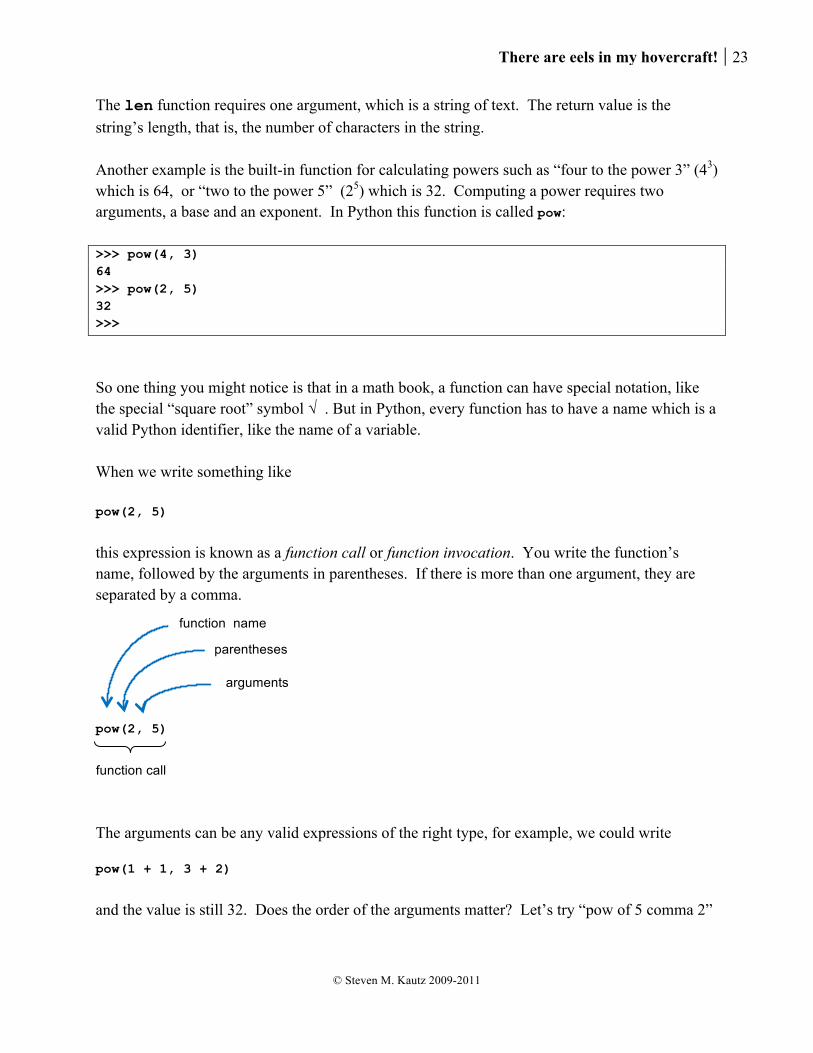
this expression is known as a function call or function invocation. You write the function’s name, followed by the arguments in parentheses. If there is more than one argument, they are separated by a comma. pow(2, 5)
The arguments can be any valid expressions of the right type, for example, we could write pow(1 + 1, 3 + 2) and the value is still 32. Does the order of the arguments matter? Let’s try “pow of 5 comma 2”
arguments
function call
function name parentheses
arguments
function call

24 Functions and input
© Steven M. Kautz 2009-2011
>>> pow(5, 2) 25
which gives us 5 to the power 2, not 2 to the power 5. So the order of the arguments is important. What happens if we don’t provide enough arguments? >>> pow(2) Traceback (most recent call last): File "<stdin>", line 1, in <module> TypeError: pow expected at least 2 arguments, got 1
Remember, we start reading error messages at the bottom. The interpreter is telling us that the pow function expects “at least 2” arguments. For a function like pow, the function call is an expression with a value that you can use. For example, you could write >>> cost = 4 * pow(2, 5) >>> print cost 128
That is, the function call pow(2, 5)is really just an expression with the value 32. Function calls can be composed just like other kinds of expressions, for example, since len(“Steve”) is 5, we can write pow(2, len("Steve")) and it still has the value 32. >>> result = pow(2, len("Steve")) >>> print result 32
It is worth noticing that we can call a function without knowing how it works. That’s why the “black box” analogy makes sense. Later we will start writing our own functions and we’ll learn in detail how they work. For now, a perfectly good explanation is that the results are calculated by gnomes.
There are eels in my hovercraft! 25
© Steven M. Kautz 2009-2011
4.3. Side-‐effects and input
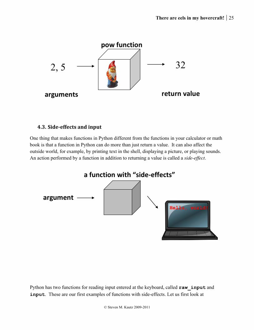
One thing that makes functions in Python different from the functions in your calculator or math book is that a function in Python can do more than just return a value. It can also affect the outside world, for example, by printing text in the shell, displaying a picture, or playing sounds. An action performed by a function in addition to returning a value is called a side-effect.
Python has two functions for reading input entered at the keyboard, called raw_input and input. These are our first examples of functions with side-effects. Let us first look at
2, 5 32
pow function
arguments return value
a function with “side-‐effects”
argument Hello, world!
26 Functions and input
© Steven M. Kautz 2009-2011
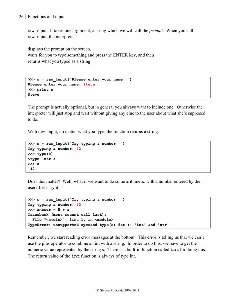
raw_input. It takes one argument, a string which we will call the prompt. When you call raw_input, the interpreter displays the prompt on the screen, waits for you to type something and press the ENTER key, and then returns what you typed as a string >>> s = raw_input("Please enter your name: ") Please enter your name: Steve >>> print s Steve
The prompt is actually optional, but in general you always want to include one. Otherwise the interpreter will just stop and wait without giving any clue to the user about what she’s supposed to do. With raw_input, no matter what you type, the function returns a string. >>> s = raw_input("Try typing a number: ") Try typing a number: 42 >>> type(s) <type 'str'> >>> s '42'
Does this matter? Well, what if we want to do some arithmetic with a number entered by the user? Let’s try it: >>> s = raw_input("Try typing a number: ") Try typing a number: 42 >>> answer = 5 + s Traceback (most recent call last): File "<stdin>", line 1, in <module> TypeError: unsupported operand type(s) for +: 'int' and 'str'
Remember, we start reading error messages at the bottom. This error is telling us that we can’t use the plus operator to combine an int with a string. In order to do this, we have to get the numeric value represented by the string s. There is a built-in function called int for doing this. The return value of the int function is always of type int.

There are eels in my hovercraft! 27
© Steven M. Kautz 2009-2011
>>> x = int("42") >>> type(x) <type 'int'> >>> x 42 >>> answer = 5 + int(s) >>> print answer 47
There is a similar function called float that converts a string such as “3.14” into a floating-point value. For input that is guaranteed to be numeric, it is usually more convenient to use the input function instead of the raw_input function. The catch is, anything you type in response to the input function has to be a valid Python expression – it can’t just be any old text. >>> value = input("Enter a number: ") Enter a number: 42 >>> value + 5 47
So what happens if we enter something that isn’t a valid expression? >>> value = input("Enter a number: ") Enter a number: boogers Traceback (most recent call last): File "<stdin>", line 1, in <module> File "<string>", line 1, in <module> NameError: name 'boogers' is not defined
A good rule of thumb is to use input for numbers, and raw_input for text.
4.4. Writing an interactive script
You are probably accustomed to interacting with applications on your computer using a graphical user interface, or “GUI”, that has windows, buttons, or other features you can control with a mouse. Writing graphical interfaces is a bit beyond the scope of this course, but we can still create interactive applications with a text-based user interface. That is, we can read input from the keyboard and print textual output on the screen. An application with a text-based interface is traditionally called a console application.
28 Functions and input
© Steven M. Kautz 2009-2011
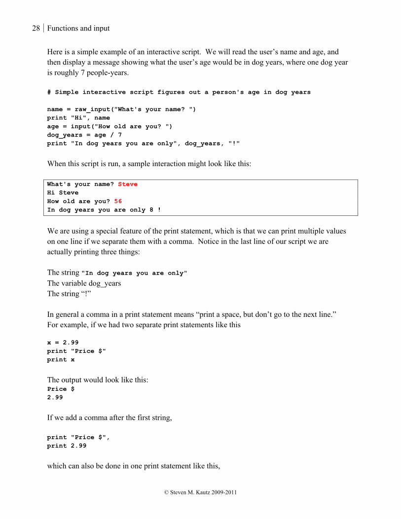
Here is a simple example of an interactive script. We will read the user’s name and age, and then display a message showing what the user’s age would be in dog years, where one dog year is roughly 7 people-years. # Simple interactive script figures out a person's age in dog years name = raw_input("What's your name? ") print "Hi", name age = input("How old are you? ") dog_years = age / 7 print "In dog years you are only", dog_years, "!"
When this script is run, a sample interaction might look like this: What's your name? Steve Hi Steve How old are you? 56 In dog years you are only 8 !
We are using a special feature of the print statement, which is that we can print multiple values on one line if we separate them with a comma. Notice in the last line of our script we are actually printing three things: The string "In dog years you are only" The variable dog_years The string “!” In general a comma in a print statement means “print a space, but don’t go to the next line.” For example, if we had two separate print statements like this x = 2.99 print "Price $" print x
The output would look like this: Price $ 2.99 If we add a comma after the first string, print "Price $", print 2.99
which can also be done in one print statement like this,
There are eels in my hovercraft! 29
© Steven M. Kautz 2009-2011
print "Price $", 2.99
The output would be Price $ 2.99
Is there some way to get rid of the space between the dollar sign and the number? We can’t do it just using print statements like this. We will need one new idea.
4.5. String concatenation and the str function
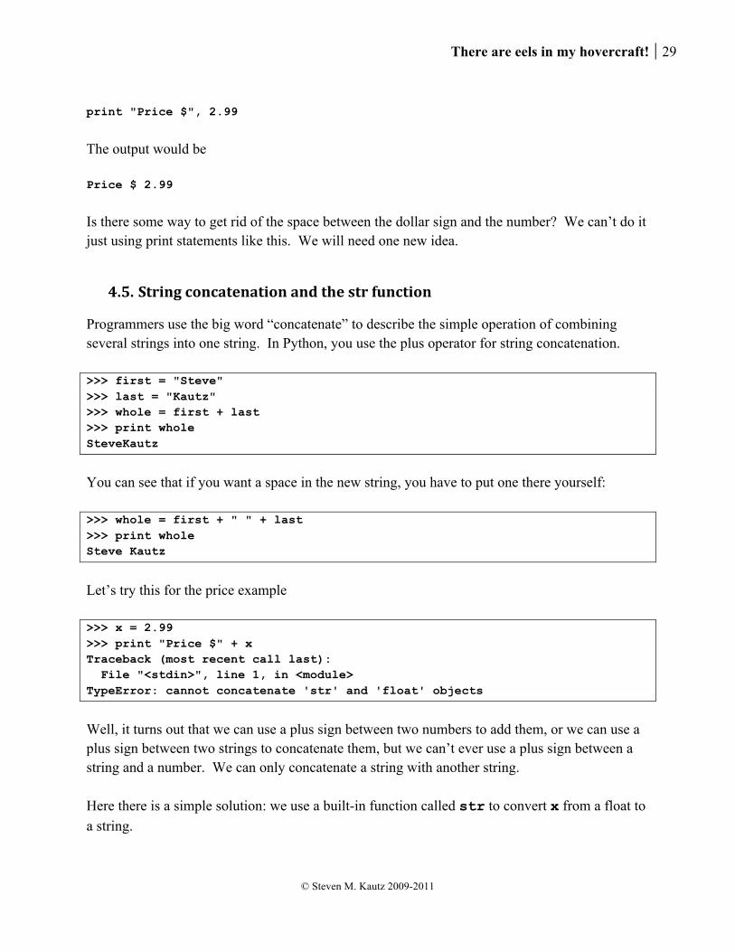
Programmers use the big word “concatenate” to describe the simple operation of combining several strings into one string. In Python, you use the plus operator for string concatenation. >>> first = "Steve" >>> last = "Kautz" >>> whole = first + last >>> print whole SteveKautz
You can see that if you want a space in the new string, you have to put one there yourself: >>> whole = first + " " + last >>> print whole Steve Kautz
Let’s try this for the price example >>> x = 2.99 >>> print "Price $" + x Traceback (most recent call last): File "<stdin>", line 1, in <module> TypeError: cannot concatenate 'str' and 'float' objects
Well, it turns out that we can use a plus sign between two numbers to add them, or we can use a plus sign between two strings to concatenate them, but we can’t ever use a plus sign between a string and a number. We can only concatenate a string with another string. Here there is a simple solution: we use a built-in function called str to convert x from a float to a string.
30 Functions and input
© Steven M. Kautz 2009-2011
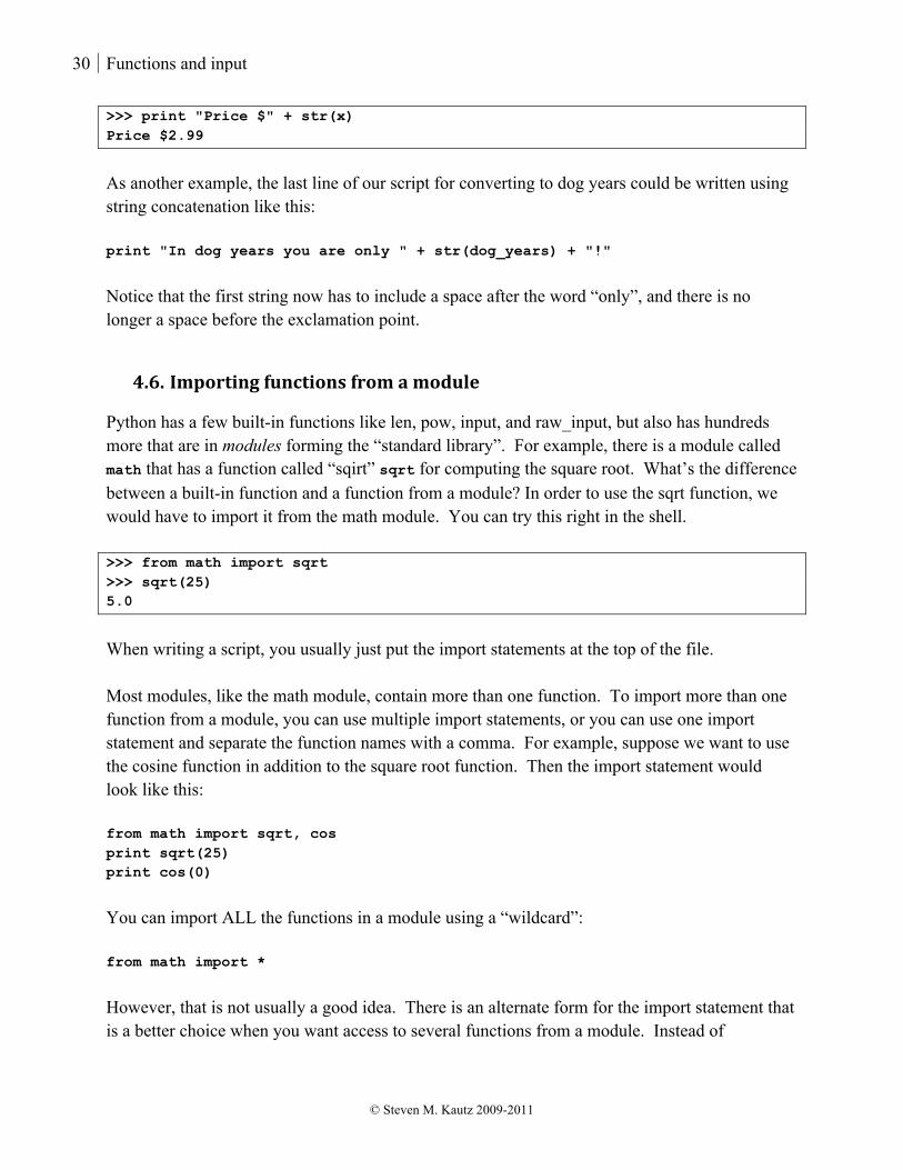
>>> print "Price $" + str(x) Price $2.99
As another example, the last line of our script for converting to dog years could be written using string concatenation like this: print "In dog years you are only " + str(dog_years) + "!"
Notice that the first string now has to include a space after the word “only”, and there is no longer a space before the exclamation point.
4.6. Importing functions from a module
Python has a few built-in functions like len, pow, input, and raw_input, but also has hundreds more that are in modules forming the “standard library”. For example, there is a module called math that has a function called “sqirt” sqrt for computing the square root. What’s the difference between a built-in function and a function from a module? In order to use the sqrt function, we would have to import it from the math module. You can try this right in the shell. >>> from math import sqrt >>> sqrt(25) 5.0
When writing a script, you usually just put the import statements at the top of the file. Most modules, like the math module, contain more than one function. To import more than one function from a module, you can use multiple import statements, or you can use one import statement and separate the function names with a comma. For example, suppose we want to use the cosine function in addition to the square root function. Then the import statement would look like this: from math import sqrt, cos print sqrt(25) print cos(0)
You can import ALL the functions in a module using a “wildcard”: from math import *
However, that is not usually a good idea. There is an alternate form for the import statement that is a better choice when you want access to several functions from a module. Instead of

There are eels in my hovercraft! 31
© Steven M. Kautz 2009-2011
importing functions by name from the module, you can just import the module. Then you can use any function in the module, as long as you precede it by the module name and a dot. import math print math.sqrt(25) print math.cos(0)
32 Conditional Statements
© Steven M. Kautz 2009-2011
5. Conditional Statements 5.1. What if Eleanor Roosevelt could fly?
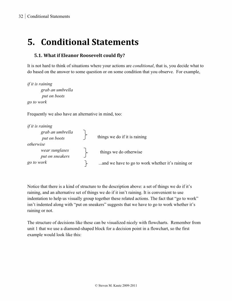
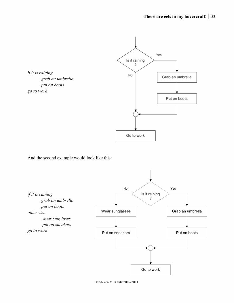
It is not hard to think of situations where your actions are conditional, that is, you decide what to do based on the answer to some question or on some condition that you observe. For example, if it is raining grab an umbrella put on boots go to work Frequently we also have an alternative in mind, too: if it is raining grab an umbrella put on boots otherwise wear sunglases put on sneakers go to work Notice that there is a kind of structure to the description above: a set of things we do if it’s raining, and an alternative set of things we do if it isn’t raining. It is convenient to use indentation to help us visually group together these related actions. The fact that “go to work” isn’t indented along with “put on sneakers” suggests that we have to go to work whether it’s raining or not. The structure of decisions like these can be visualized nicely with flowcharts. Remember from unit 1 that we use a diamond-shaped block for a decision point in a flowchart, so the first example would look like this:
things we do if it is raining
things we do otherwise
...and we have to go to work whether it’s raining or not!
There are eels in my hovercraft! 33
© Steven M. Kautz 2009-2011
if it is raining grab an umbrella put on boots go to work And the second example would look like this: if it is raining grab an umbrella put on boots otherwise wear sunglases put on sneakers go to work
Is it raining?
No
Grab an umbrella
Go to work
Put on boots
Wear sunglasses
Put on sneakers
Yes

34 Conditional Statements
© Steven M. Kautz 2009-2011
The flowcharts make one thing very clear, anyway. There are two branches or paths through the diagram, and you’ll do the things on the “Yes” branch, OR you’ll do the things on the “No” branch, but there’s no possible path along the arrows in which you do the things on both branches. Also notice the small circle where the “Yes” and “No” branches come back together. That is an important feature that reflects the way that conditional statements are used in programming. You’ll take one of two alternative paths that have different actions on them, but both paths MUST eventually end up at the same point again.
5.2. Boolean expressions
As you might expect, we want to be able to write statements in Python representing conditional actions. What’s a “condition”, anyway? By “condition”, we just mean an expression whose value is either true or false. For example, what if you type an expression like “2 < 3” in the shell? >>> 2 < 3 True >>>
Well, that sort of makes sense. Let’s try another one. >>> x = 42 >>> x > 100 False >>>
We know that every value has a type, so what is the type of an expression like 2 < 3? It obviously isn’t an int, a float, or a string, the three types we know about so far. We can find out with the type function. >>> type(2 < 3) <type 'bool'>
This is something we haven’t seen before. It turns out that “bool” is short for “boolean”, a type that has just two possible values, represented by the Python literals True and False. We can write simple boolean expressions using the relational operators for greater-than and less-than as

There are eels in my hovercraft! 35
© Steven M. Kautz 2009-2011
in the examples above. There are six relational operators in all. You’ve seen them all in math classes, but in Python we have to use slightly different symbols, as shown in the table below. Meaning Mathematical symbol Python symbol Less than < <
Greater than > >
Less than or equal to ≤ <=
Greater than or equal to ≥ >=
Not equal to ≠ !=
Equal to = ==
That last one is somewhat curious. Remember, the equals sign is not an equals sign in Python, it is the assignment operator. So to test whether two expressions are equal, we need a different symbol. Like several other programming languages, Python uses a double equals sign for this purpose: We read the first line as “x gets the value 42”, which is a statement that changes the value of x. We read the second line as “x is equal to 43”, which is an expression with the value False. It doesn’t change the value of x. >>> x = 42 >>> x == 43 False >>> x == 42 True >>> x != 100 True >>> Be careful! Using an assignment operator, that is, a single equals sign, when you really want to check equality is definitely one of the all-time top ten programming errors. Notice that if we accidentally wrote x = 43 in the second line above, it wouldn’t check whether x was equal to 43, it would change the value of x to be 43!
5.3. Conditional statements
Let’s start with an example. Here’s a short script that reads an exam score from a user and then prints a brief response.
36 Conditional Statements
© Steven M. Kautz 2009-2011
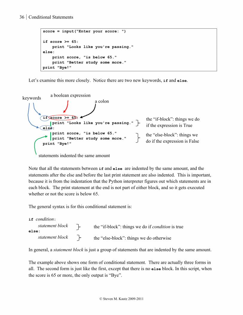
score = input("Enter your score: ") if score >= 65: print "Looks like you're passing." else: print score, "is below 65." print "Better study some more." print "Bye!"
Let’s examine this more closely. Notice there are two new keywords, if and else.
if score >= 65: print "Looks like you're passing." else: print score, "is below 65." print "Better study some more." print "Bye!"
Note that all the statements between if and else are indented by the same amount, and the statements after the else and before the last print statement are also indented. This is important, because it is from the indentation that the Python interpreter figures out which statements are in each block. The print statement at the end is not part of either block, and so it gets executed whether or not the score is below 65. The general syntax is for this conditional statement is: if condition: statement block else:
statement block In general, a statement block is just a group of statements that are indented by the same amount. The example above shows one form of conditional statement. There are actually three forms in all. The second form is just like the first, except that there is no else block. In this script, when the score is 65 or more, the only output is “Bye”.
the “if-block”: things we do if condition is true
the “else-block”: things we do otherwise
keywords a boolean expression a colon
statements indented the same amount
the “if-block”: things we do if the expression is True
the “else-block”: things we do if the expression is False
There are eels in my hovercraft! 37
© Steven M. Kautz 2009-2011
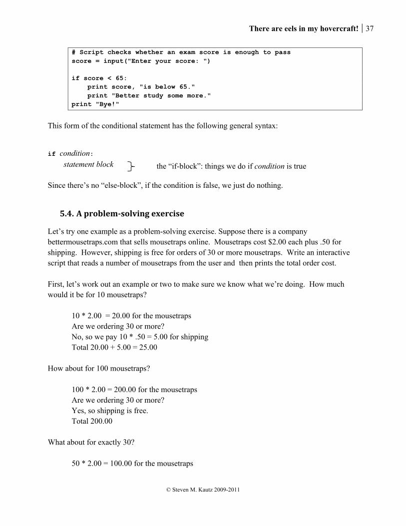
# Script checks whether an exam score is enough to pass score = input("Enter your score: ") if score < 65: print score, "is below 65." print "Better study some more." print "Bye!"
This form of the conditional statement has the following general syntax:
if condition: statement block Since there’s no “else-block”, if the condition is false, we just do nothing.
5.4. A problem-‐solving exercise
Let’s try one example as a problem-solving exercise. Suppose there is a company bettermousetraps.com that sells mousetraps online. Mousetraps cost $2.00 each plus .50 for shipping. However, shipping is free for orders of 30 or more mousetraps. Write an interactive script that reads a number of mousetraps from the user and then prints the total order cost. First, let’s work out an example or two to make sure we know what we’re doing. How much would it be for 10 mousetraps?
10 * 2.00 = 20.00 for the mousetraps Are we ordering 30 or more? No, so we pay 10 * .50 = 5.00 for shipping Total 20.00 + 5.00 = 25.00
How about for 100 mousetraps?
100 * 2.00 = 200.00 for the mousetraps Are we ordering 30 or more? Yes, so shipping is free. Total 200.00
What about for exactly 30?
50 * 2.00 = 100.00 for the mousetraps
the “if-block”: things we do if condition is true
38 Conditional Statements
© Steven M. Kautz 2009-2011
Are we ordering 30 or more? Yes, so shipping is free. Total 100.00
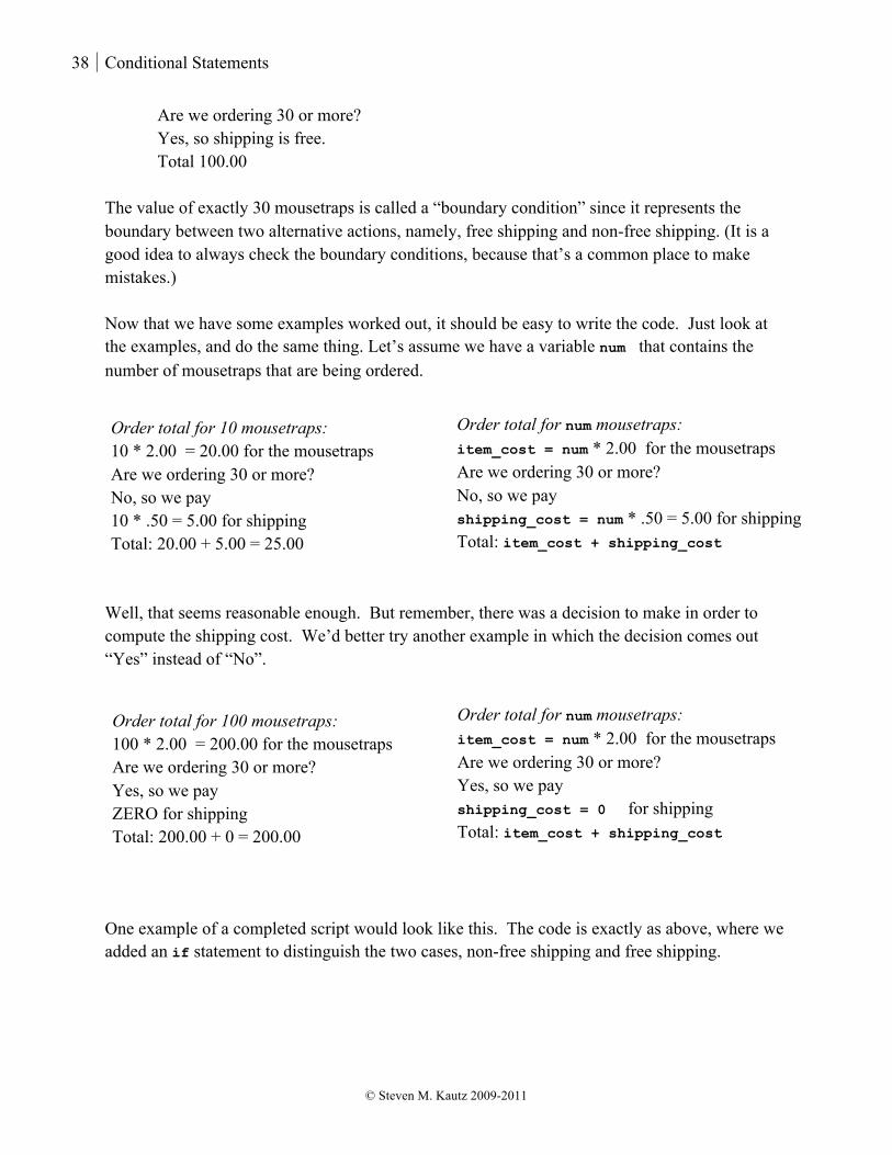
The value of exactly 30 mousetraps is called a “boundary condition” since it represents the boundary between two alternative actions, namely, free shipping and non-free shipping. (It is a good idea to always check the boundary conditions, because that’s a common place to make mistakes.) Now that we have some examples worked out, it should be easy to write the code. Just look at the examples, and do the same thing. Let’s assume we have a variable num that contains the number of mousetraps that are being ordered.
Well, that seems reasonable enough. But remember, there was a decision to make in order to compute the shipping cost. We’d better try another example in which the decision comes out “Yes” instead of “No”.
One example of a completed script would look like this. The code is exactly as above, where we added an if statement to distinguish the two cases, non-free shipping and free shipping.
Order total for 10 mousetraps: 10 * 2.00 = 20.00 for the mousetraps Are we ordering 30 or more? No, so we pay 10 * .50 = 5.00 for shipping Total: 20.00 + 5.00 = 25.00
Order total for num mousetraps: item_cost = num * 2.00 for the mousetraps Are we ordering 30 or more? No, so we pay shipping_cost = num * .50 = 5.00 for shipping Total: item_cost + shipping_cost
Order total for 100 mousetraps: 100 * 2.00 = 200.00 for the mousetraps Are we ordering 30 or more? Yes, so we pay ZERO for shipping Total: 200.00 + 0 = 200.00
Order total for num mousetraps: item_cost = num * 2.00 for the mousetraps Are we ordering 30 or more? Yes, so we pay shipping_cost = 0 for shipping Total: item_cost + shipping_cost
There are eels in my hovercraft! 39
© Steven M. Kautz 2009-2011
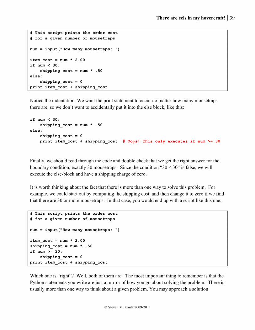
# This script prints the order cost # for a given number of mousetraps num = input("How many mousetraps: ") item_cost = num * 2.00 if num < 30: shipping_cost = num * .50 else: shipping_cost = 0 print item_cost + shipping_cost
Notice the indentation. We want the print statement to occur no matter how many mousetraps there are, so we don’t want to accidentally put it into the else block, like this: if num < 30: shipping_cost = num * .50 else: shipping_cost = 0 print item_cost + shipping_cost # Oops! This only executes if num >= 30 Finally, we should read through the code and double check that we get the right answer for the boundary condition, exactly 30 mousetraps. Since the condition “30 < 30” is false, we will execute the else-block and have a shipping charge of zero. It is worth thinking about the fact that there is more than one way to solve this problem. For example, we could start out by computing the shipping cost, and then change it to zero if we find that there are 30 or more mousetraps. In that case, you would end up with a script like this one. # This script prints the order cost # for a given number of mousetraps num = input("How many mousetraps: ") item_cost = num * 2.00 shipping_cost = num * .50 if num >= 30: shipping_cost = 0 print item_cost + shipping_cost
Which one is “right”? Well, both of them are. The most important thing to remember is that the Python statements you write are just a mirror of how you go about solving the problem. There is usually more than one way to think about a given problem. You may approach a solution
40 Conditional Statements
© Steven M. Kautz 2009-2011
differently than someone else, but as long as you faithfully translate the steps of your strategy into Python statements you’ll end up with a working program.
There are eels in my hovercraft! 41
© Steven M. Kautz 2009-2011
6. Nested conditionals 6.1. Nested conditionals
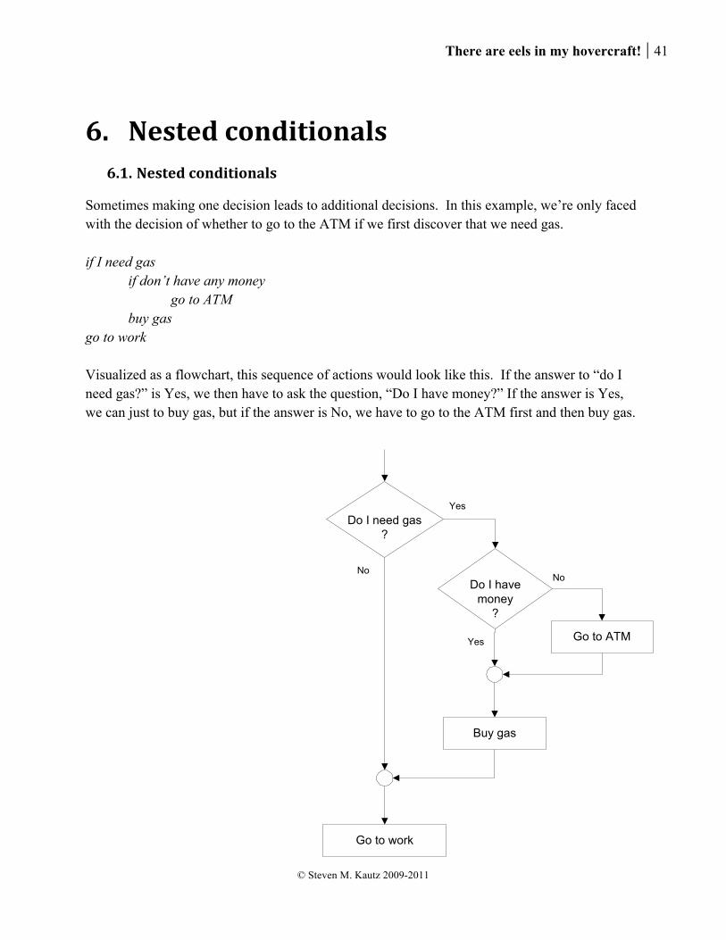
Sometimes making one decision leads to additional decisions. In this example, we’re only faced with the decision of whether to go to the ATM if we first discover that we need gas. if I need gas if don’t have any money go to ATM buy gas go to work Visualized as a flowchart, this sequence of actions would look like this. If the answer to “do I need gas?” is Yes, we then have to ask the question, “Do I have money?” If the answer is Yes, we can just to buy gas, but if the answer is No, we have to go to the ATM first and then buy gas.
Do I need gas?
No
Yes
Go to ATM
Do I have money
?
No
Yes
Buy gas
Go to work
42 Nested conditionals
© Steven M. Kautz 2009-2011
How do we express something like this in Python? If you look at the two general forms of an if-statement we have seen so far: if condition: statement block else:
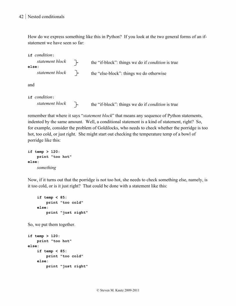
statement block and if condition: statement block remember that where it says “statement block” that means any sequence of Python statements, indented by the same amount. Well, a conditional statement is a kind of statement, right? So, for example, consider the problem of Goldilocks, who needs to check whether the porridge is too hot, too cold, or just right. She might start out checking the temperature temp of a bowl of porridge like this: if temp > 120: print "too hot" else:
something Now, if it turns out that the porridge is not too hot, she needs to check something else, namely, is it too cold, or is it just right? That could be done with a statement like this: if temp < 85: print "too cold" else: print "just right"
So, we put them together. if temp > 120: print "too hot" else: if temp < 85: print "too cold" else: print "just right"
the “if-block”: things we do if condition is true
the “else-block”: things we do otherwise
the “if-block”: things we do if condition is true

There are eels in my hovercraft! 43
© Steven M. Kautz 2009-2011
Notice there are now two “indentation levels”, since the entire statement “if temp < 85...” must itself be indented to be part of the outer “else-block”. if temp > 120: print "too hot" else: if temp < 85: print "too cold" else: print "just right"
6.2. A more complex example
Here’s another example. Suppose we want to convert scores to letter grades, using the following scale: if the score is 90 or above it’s an “A”: otherwise, if the score is 80 or above it’s a “B”; otherwise if the score is 70 or above is’s a “C”; otherwise it’s an “F”. One thing that helps to think about a problem like this is to first try to write out the decision algorithm in “pseudocode”. Pseudocode is a way of describing an algorithm informally that is sort of halfway between English and actual code, using indentation to group actions together. When writing pseudocode, we’re thinking about eventually writing actual code, so we try to think in terms of “if” and “else” blocks. It might look something like this: if the score is 90 or above grade is an “A” else if the score is 80 or above grade is a “B” else if the score is 70 or above grade is a “C” else grade is an “F”
indentation level for outer if and else blocks
indentation level for inner if and else blocks
44 Nested conditionals
© Steven M. Kautz 2009-2011
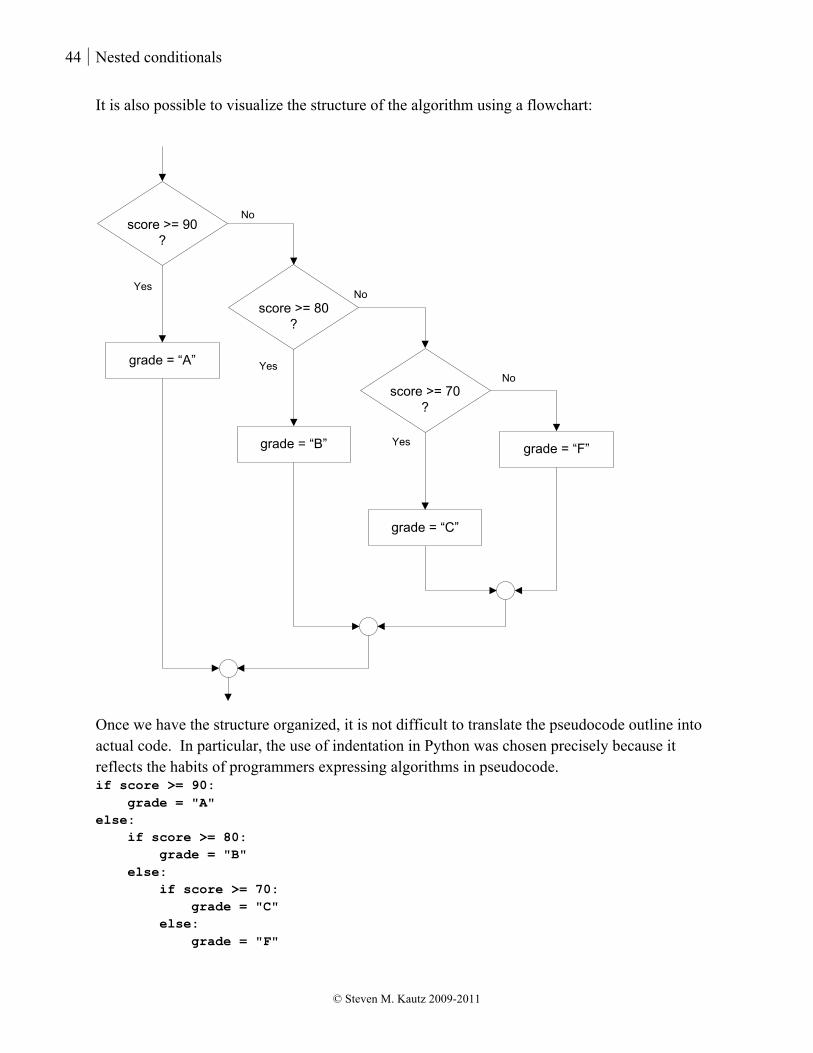
It is also possible to visualize the structure of the algorithm using a flowchart:
score >= 90?
Yes
No
No
Yes
score >= 80?
score >= 70?
grade = “A”
grade = “B”
grade = “C”
grade = “F”
No
Yes
Once we have the structure organized, it is not difficult to translate the pseudocode outline into actual code. In particular, the use of indentation in Python was chosen precisely because it reflects the habits of programmers expressing algorithms in pseudocode. if score >= 90: grade = "A" else: if score >= 80: grade = "B" else: if score >= 70: grade = "C" else: grade = "F"

There are eels in my hovercraft! 45
© Steven M. Kautz 2009-2011
There are now three indentation levels! Let’s trace through an example: Suppose the score is 75. Is the score above 90? No, so we skip the outer “if” block and enter the outer “else” block: if score >= 80: grade = "B" else: if score >= 70: grade = "C" else: grade = "F"
Is the grade above 80? No, so we skip the “if” block and enter the “else” block: if score >= 70: grade = "C" else: grade = "F"
Is the grade above 70? Yes, so we execute the “if” block and assign a grade of “C”, skipping the else block. The grade ends up as a “C”. The nesting of conditional statements here is important. The condition if score >= 80: grade = "B"
only makes sense once we already know that the score is not above 90. For example what would happen if we tried writing the code like this? if score >= 90: grade = "A" if score >= 80: grade = "B" if score >= 70: grade = "C" else: grade = "F"

46 Nested conditionals
© Steven M. Kautz 2009-2011
Let’s see what happens to someone with a score of 95. 95 is greater than or equal to 90, so grade is set to “A”. Then, we continue on to the next “if” statement. Since 95 is greater than or equal to 80, we now set the grade to “B”. Next, we check that 95 is greater than or equal to 70, and then set the grade to “C”. Obviously that’s not what your instructor intended!
6.3. The elif keyword
Sometimes, though not always, you find that a nested conditional is written so that immediately after an “else” there is another if, as we saw in the first example: if temp > 120: print "too hot" else: if temp < 85: print "too cold" else: print "just right"
In situations like this when there is an ”else” right after an “if”, you can use a special keyword elif in order to “contract” the if and the else onto the same line. This is the third form of conditional statement. The possible advantage of using elif is that it reduces the number of indentation levels and makes the code easier to read. The Goldilocks example would look like this: if temp > 120: print "too hot" elif temp < 85: print "too cold" else: print "just right"
The letter grade example would look like this: if score >= 90: grade = "A" elif score >= 80: grade = "B" elif score >= 70: grade = "C" else: grade = "F"
There are eels in my hovercraft! 47
© Steven M. Kautz 2009-2011
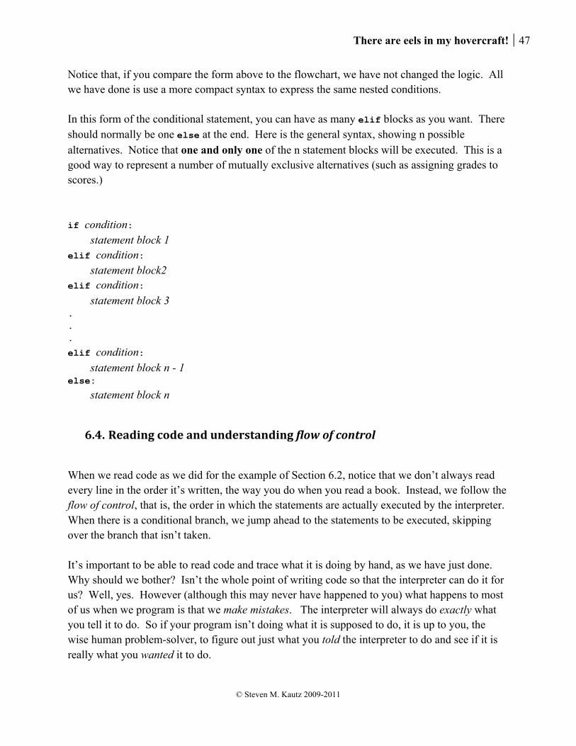
Notice that, if you compare the form above to the flowchart, we have not changed the logic. All we have done is use a more compact syntax to express the same nested conditions. In this form of the conditional statement, you can have as many elif blocks as you want. There should normally be one else at the end. Here is the general syntax, showing n possible alternatives. Notice that one and only one of the n statement blocks will be executed. This is a good way to represent a number of mutually exclusive alternatives (such as assigning grades to scores.) if condition: statement block 1 elif condition: statement block2 elif condition: statement block 3 . . .
elif condition: statement block n - 1 else:
statement block n
6.4. Reading code and understanding flow of control
When we read code as we did for the example of Section 6.2, notice that we don’t always read every line in the order it’s written, the way you do when you read a book. Instead, we follow the flow of control, that is, the order in which the statements are actually executed by the interpreter. When there is a conditional branch, we jump ahead to the statements to be executed, skipping over the branch that isn’t taken. It’s important to be able to read code and trace what it is doing by hand, as we have just done. Why should we bother? Isn’t the whole point of writing code so that the interpreter can do it for us? Well, yes. However (although this may never have happened to you) what happens to most of us when we program is that we make mistakes. The interpreter will always do exactly what you tell it to do. So if your program isn’t doing what it is supposed to do, it is up to you, the wise human problem-solver, to figure out just what you told the interpreter to do and see if it is really what you wanted it to do.
48 Writing our own functions
© Steven M. Kautz 2009-2011
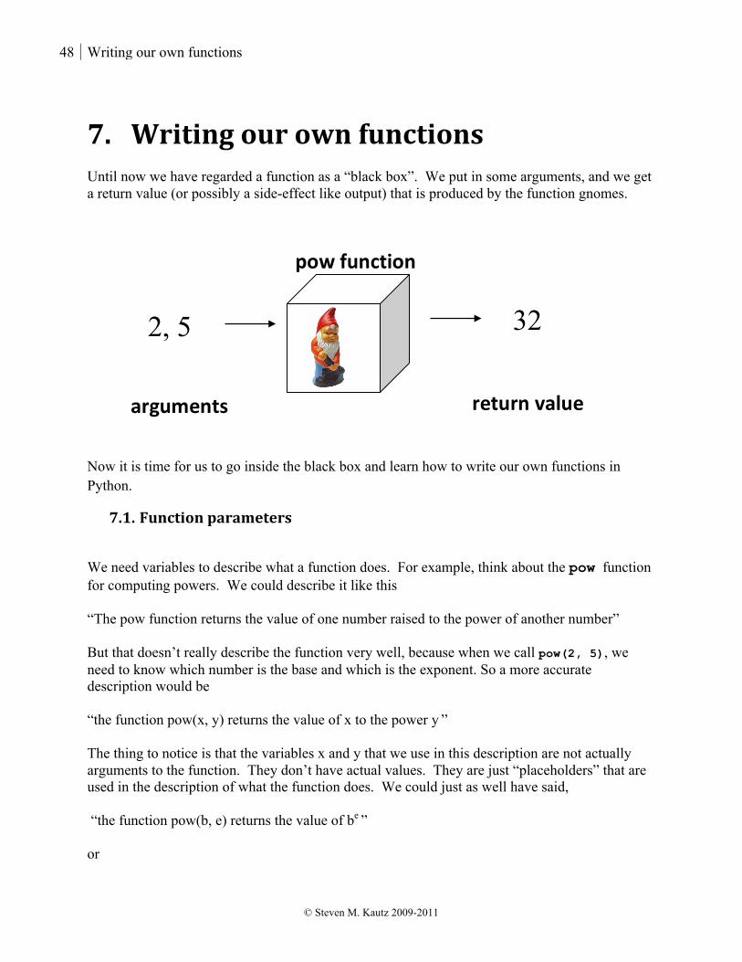
7. Writing our own functions Until now we have regarded a function as a “black box”. We put in some arguments, and we get a return value (or possibly a side-effect like output) that is produced by the function gnomes.
Now it is time for us to go inside the black box and learn how to write our own functions in Python.
7.1. Function parameters
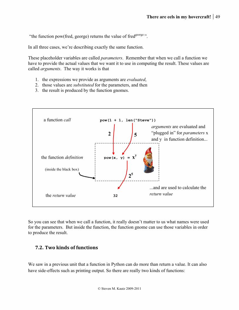
We need variables to describe what a function does. For example, think about the pow function for computing powers. We could describe it like this “The pow function returns the value of one number raised to the power of another number” But that doesn’t really describe the function very well, because when we call pow(2, 5), we need to know which number is the base and which is the exponent. So a more accurate description would be “the function pow(x, y) returns the value of x to the power y ” The thing to notice is that the variables x and y that we use in this description are not actually arguments to the function. They don’t have actual values. They are just “placeholders” that are used in the description of what the function does. We could just as well have said, “the function pow(b, e) returns the value of be ” or
2, 5 32
pow function
arguments return value
There are eels in my hovercraft! 49
© Steven M. Kautz 2009-2011
“the function pow(fred, george) returns the value of fredgeorge ”. In all three cases, we’re describing exactly the same function. These placeholder variables are called parameters. Remember that when we call a function we have to provide the actual values that we want it to use in computing the result. These values are called arguments. The way it works is that
1. the expressions we provide as arguments are evaluated, 2. those values are substituted for the parameters, and then 3. the result is produced by the function gnomes.
So you can see that when we call a function, it really doesn’t matter to us what names were used for the parameters. But inside the function, the function gnome can use those variables in order to produce the result.
7.2. Two kinds of functions
We saw in a previous unit that a function in Python can do more than return a value. It can also have side-effects such as printing output. So there are really two kinds of functions:
a function call pow(1 + 1, len("Steve"))
the function definition pow(x, y) = xy
the return value 32
5 2 arguments are evaluated and “plugged in” for parameters x and y in function definition...
...and are used to calculate the return value
25 (inside the black box)
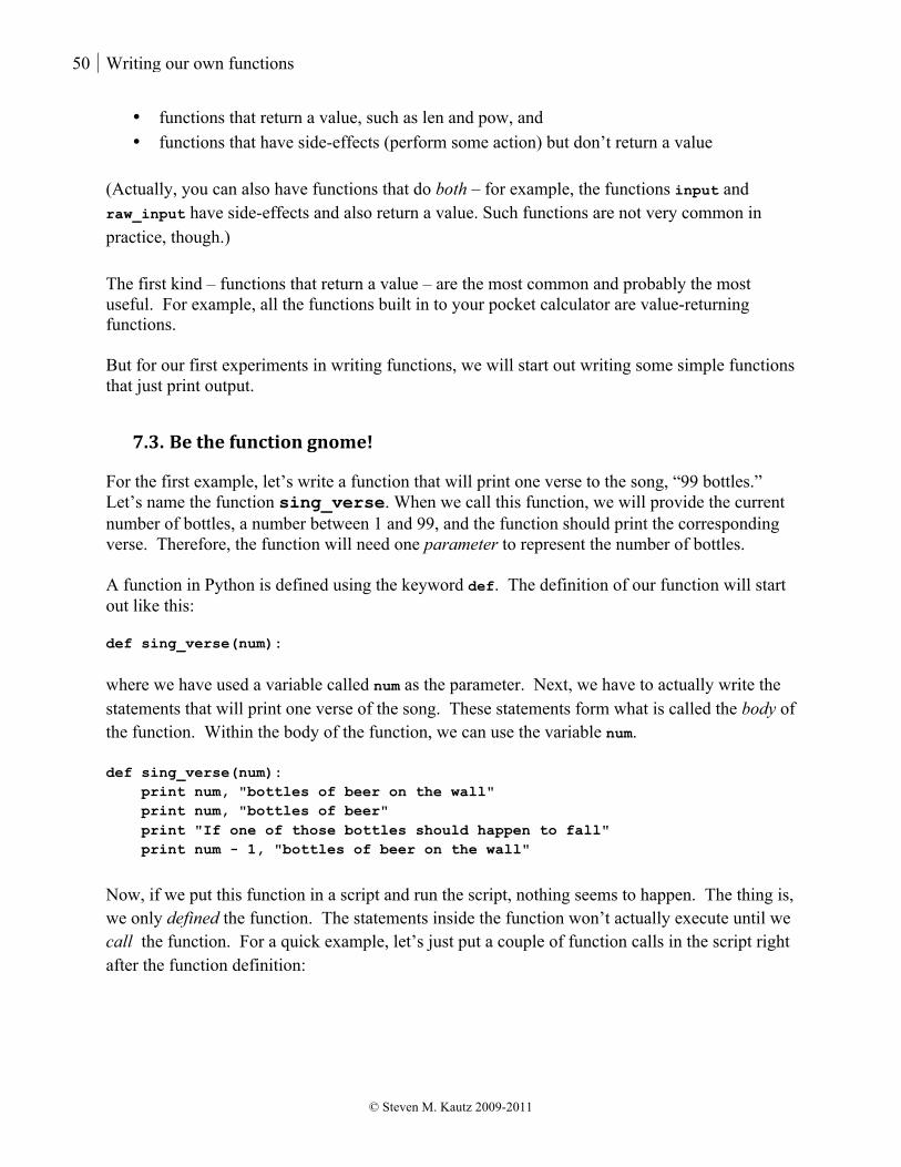
50 Writing our own functions
© Steven M. Kautz 2009-2011
• functions that return a value, such as len and pow, and • functions that have side-effects (perform some action) but don’t return a value
(Actually, you can also have functions that do both – for example, the functions input and raw_input have side-effects and also return a value. Such functions are not very common in practice, though.) The first kind – functions that return a value – are the most common and probably the most useful. For example, all the functions built in to your pocket calculator are value-returning functions. But for our first experiments in writing functions, we will start out writing some simple functions that just print output.
7.3. Be the function gnome!
For the first example, let’s write a function that will print one verse to the song, “99 bottles.” Let’s name the function sing_verse. When we call this function, we will provide the current number of bottles, a number between 1 and 99, and the function should print the corresponding verse. Therefore, the function will need one parameter to represent the number of bottles. A function in Python is defined using the keyword def. The definition of our function will start out like this: def sing_verse(num):
where we have used a variable called num as the parameter. Next, we have to actually write the statements that will print one verse of the song. These statements form what is called the body of the function. Within the body of the function, we can use the variable num. def sing_verse(num): print num, "bottles of beer on the wall" print num, "bottles of beer" print "If one of those bottles should happen to fall" print num - 1, "bottles of beer on the wall"
Now, if we put this function in a script and run the script, nothing seems to happen. The thing is, we only defined the function. The statements inside the function won’t actually execute until we call the function. For a quick example, let’s just put a couple of function calls in the script right after the function definition:
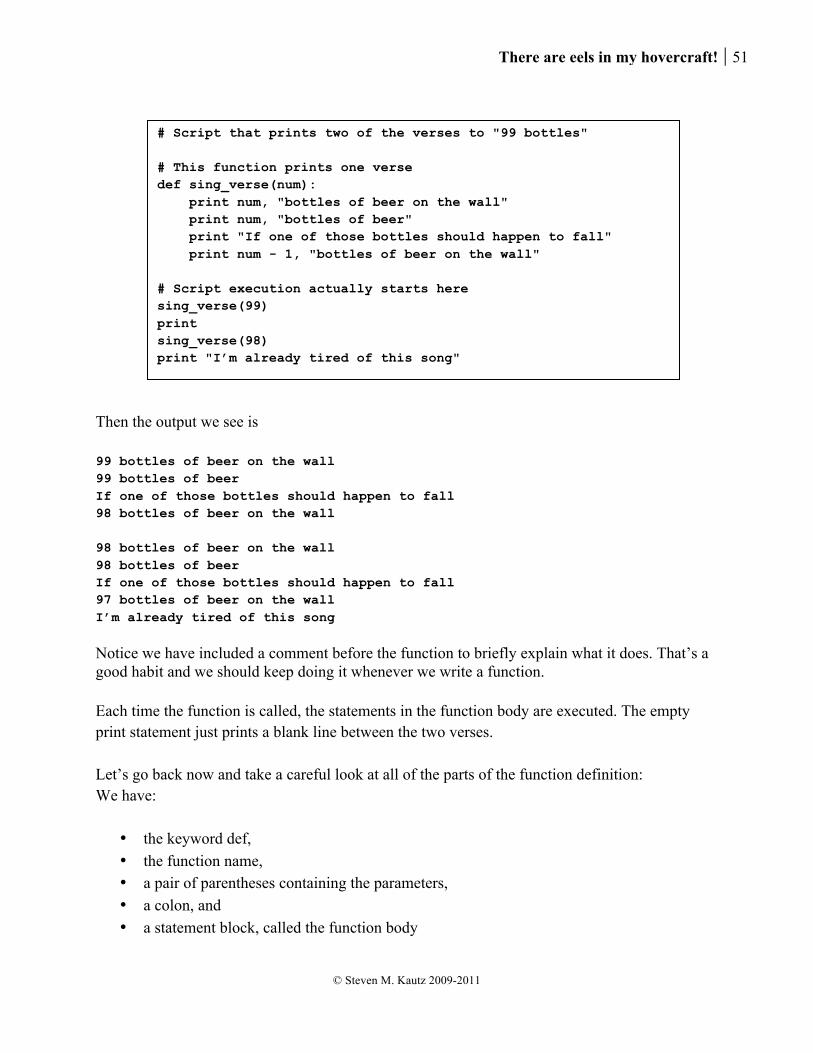
There are eels in my hovercraft! 51
© Steven M. Kautz 2009-2011
Then the output we see is 99 bottles of beer on the wall 99 bottles of beer If one of those bottles should happen to fall 98 bottles of beer on the wall 98 bottles of beer on the wall 98 bottles of beer If one of those bottles should happen to fall 97 bottles of beer on the wall I’m already tired of this song Notice we have included a comment before the function to briefly explain what it does. That’s a good habit and we should keep doing it whenever we write a function. Each time the function is called, the statements in the function body are executed. The empty print statement just prints a blank line between the two verses. Let’s go back now and take a careful look at all of the parts of the function definition: We have:
• the keyword def, • the function name, • a pair of parentheses containing the parameters, • a colon, and • a statement block, called the function body
# Script that prints two of the verses to "99 bottles" # This function prints one verse def sing_verse(num): print num, "bottles of beer on the wall" print num, "bottles of beer" print "If one of those bottles should happen to fall" print num - 1, "bottles of beer on the wall" # Script execution actually starts here sing_verse(99) print sing_verse(98) print "I’m already tired of this song"
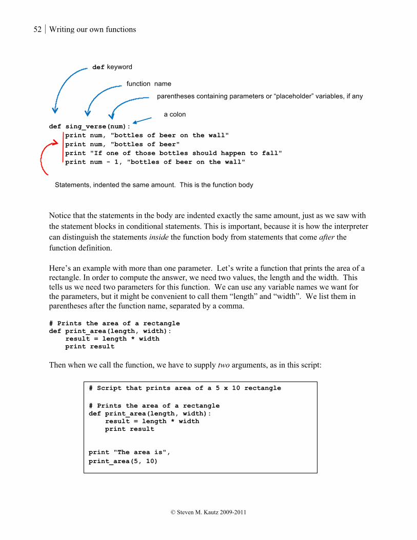
52 Writing our own functions
© Steven M. Kautz 2009-2011
def sing_verse(num): print num, "bottles of beer on the wall" print num, "bottles of beer" print "If one of those bottles should happen to fall" print num - 1, "bottles of beer on the wall"
Notice that the statements in the body are indented exactly the same amount, just as we saw with the statement blocks in conditional statements. This is important, because it is how the interpreter can distinguish the statements inside the function body from statements that come after the function definition. Here’s an example with more than one parameter. Let’s write a function that prints the area of a rectangle. In order to compute the answer, we need two values, the length and the width. This tells us we need two parameters for this function. We can use any variable names we want for the parameters, but it might be convenient to call them “length” and “width”. We list them in parentheses after the function name, separated by a comma. # Prints the area of a rectangle def print_area(length, width): result = length * width print result Then when we call the function, we have to supply two arguments, as in this script:
def keyword
function name parentheses containing parameters or “placeholder” variables, if any
a colon
Statements, indented the same amount. This is the function body
# Script that prints area of a 5 x 10 rectangle # Prints the area of a rectangle def print_area(length, width): result = length * width print result print "The area is", print_area(5, 10)
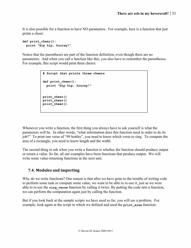
There are eels in my hovercraft! 53
© Steven M. Kautz 2009-2011
It is also possible for a function to have NO parameters. For example, here is a function that just prints a cheer: def print_cheer(): print "Hip hip, hooray!"
Notice that the parentheses are part of the function definition, even though there are no parameters. And when you call a function like this, you also have to remember the parentheses. For example, this script would print three cheers: Whenever you write a function, the first thing you always have to ask yourself is what the parameters will be. In other words, “what information does this function need in order to do its job?” To print one verse of “99 bottles”, you need to know which verse to sing. To compute the area of a rectangle, you need to know length and the width. The second thing to ask when you write a function is whether the function should produce output or return a value. So far, all our examples have been functions that produce output. We will write some value-returning functions in the next unit.
7.4. Modules and importing
Why do we write functions? One reason is that after we have gone to the trouble of writing code to perform some task or compute some value, we want to be able to re-use it, just as we were able to re-use the sing_verse function by calling it twice. By putting the code into a function, we can perform the computation again just by calling the function. But if you look back at the sample scripts we have used so far, you will see a problem. For example, look again at the script in which we defined and used the print_area function:
# Script that prints three cheers def print_cheer(): print "Hip hip, hooray!" print_cheer() print_cheer() print_cheer()

54 Writing our own functions
© Steven M. Kautz 2009-2011
What if we want to use this function in a different script? The problem here is that we are calling the function in the same script in which we’ve defined it. That makes it hard to re-use the function somewhere else. In general, we want to be able to define a function in one script, and make it available to be used in a different script - possibly in many others, if it is a particularly useful function. Let’s try it. As an experiment, suppose we just take out the call to print_area and put it in a different script. Assume that we have these two files, my_functions.py and test.py, stored in the same directory. my_functions.py test.py So far so good. But when we run the script test.py, we get the message NameError: name 'print_area' is not defined What’s up with that? The thing is, we have to tell the interpreter where to find the print_area function. We do that by putting an import statement at the top of the file test.py:
# Script that prints area of a 5 x 10 rectangle # Prints the area of a rectangle def print_area(length, width): result = length * width print result print "The area is", print_area(5, 10)
Definition of function
Use of function
# Module containing definition # of area function # Prints the area of a rectangle def print_area(length, width): result = length * width print result
# Script that prints area of # a 5 x 10 rectangle print "The area is", print_area(5, 10)
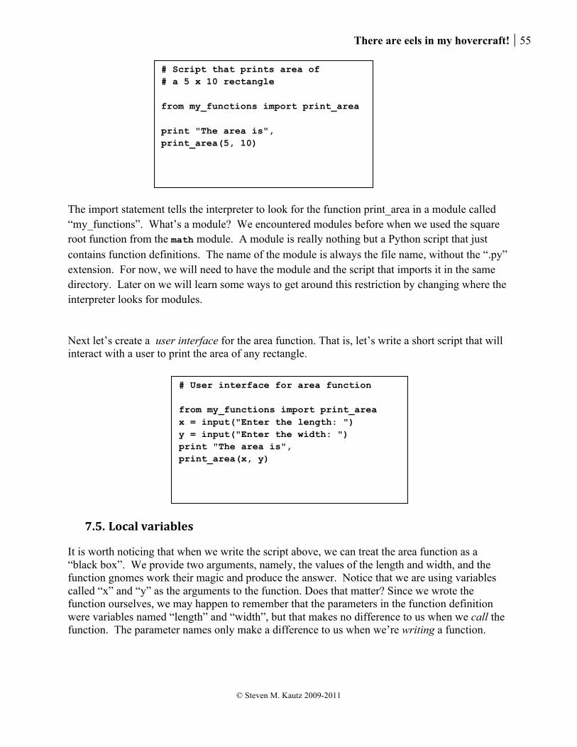
There are eels in my hovercraft! 55
© Steven M. Kautz 2009-2011
The import statement tells the interpreter to look for the function print_area in a module called “my_functions”. What’s a module? We encountered modules before when we used the square root function from the math module. A module is really nothing but a Python script that just contains function definitions. The name of the module is always the file name, without the “.py” extension. For now, we will need to have the module and the script that imports it in the same directory. Later on we will learn some ways to get around this restriction by changing where the interpreter looks for modules. Next let’s create a user interface for the area function. That is, let’s write a short script that will interact with a user to print the area of any rectangle.
7.5. Local variables
It is worth noticing that when we write the script above, we can treat the area function as a “black box”. We provide two arguments, namely, the values of the length and width, and the function gnomes work their magic and produce the answer. Notice that we are using variables called “x” and “y” as the arguments to the function. Does that matter? Since we wrote the function ourselves, we may happen to remember that the parameters in the function definition were variables named “length” and “width”, but that makes no difference to us when we call the function. The parameter names only make a difference to us when we’re writing a function.
# Script that prints area of # a 5 x 10 rectangle from my_functions import print_area print "The area is", print_area(5, 10)
# User interface for area function from my_functions import print_area x = input("Enter the length: ") y = input("Enter the width: ") print "The area is", print_area(x, y)
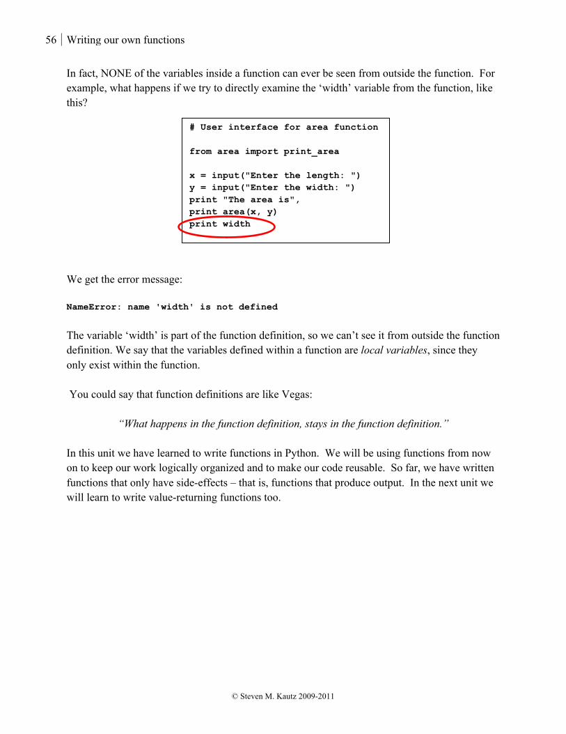
56 Writing our own functions
© Steven M. Kautz 2009-2011
In fact, NONE of the variables inside a function can ever be seen from outside the function. For example, what happens if we try to directly examine the ‘width’ variable from the function, like this? We get the error message: NameError: name 'width' is not defined
The variable ‘width’ is part of the function definition, so we can’t see it from outside the function definition. We say that the variables defined within a function are local variables, since they only exist within the function. You could say that function definitions are like Vegas:
“What happens in the function definition, stays in the function definition.” In this unit we have learned to write functions in Python. We will be using functions from now on to keep our work logically organized and to make our code reusable. So far, we have written functions that only have side-effects – that is, functions that produce output. In the next unit we will learn to write value-returning functions too.
# User interface for area function from area import print_area x = input("Enter the length: ") y = input("Enter the width: ") print "The area is", print_area(x, y) print width

There are eels in my hovercraft! 57
© Steven M. Kautz 2009-2011
8. Value-‐returning functions Last time we talked about the fact that when we define a function, we start by asking ourselves two questions:
• What are the parameters, that is, what pieces of information will this function need in order to do its job?
• Should the function produce its own output, or should it return a value? So far we have only written functions that produce output. Now we are going to learn how to write value-returning functions.
8.1. Value-‐returning functions
As an example to start with, remember that last time we wrote a function that computes the area of a rectangle, given the length and width. # Prints the area of a rectangle def print_area(length, width): result = length * width print result Now, what if we don’t just want to print the area, but we want to use the value in another calculation? For example, suppose we are going to put carpet in a 10 by 12 foot room, and the carpet is $1.50 per square foot. We could try writing a statement like this to determine the cost of the carpet: carpet_cost = 1.50 * print_area(10, 12)
But something goes very wrong here. The function call print_area(10, 12) doesn’t actually give us the value of the area, it just prints the value on the screen! If we want to do something with the value other than printing it on the screen, we need to write a different kind of function. Instead of printing output, what we need is a return statement to give the function call a value. # Returns the area of a rectangle def area(length, width): result = length * width return result
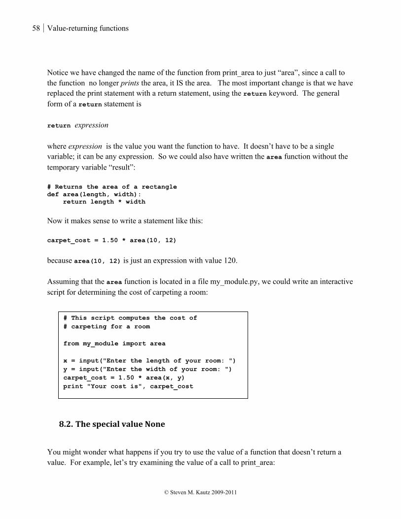
58 Value-returning functions
© Steven M. Kautz 2009-2011
Notice we have changed the name of the function from print_area to just “area”, since a call to the function no longer prints the area, it IS the area. The most important change is that we have replaced the print statement with a return statement, using the return keyword. The general form of a return statement is return expression where expression is the value you want the function to have. It doesn’t have to be a single variable; it can be any expression. So we could also have written the area function without the temporary variable “result”: # Returns the area of a rectangle def area(length, width): return length * width Now it makes sense to write a statement like this: carpet_cost = 1.50 * area(10, 12) because area(10, 12) is just an expression with value 120. Assuming that the area function is located in a file my_module.py, we could write an interactive script for determining the cost of carpeting a room:
8.2. The special value None
You might wonder what happens if you try to use the value of a function that doesn’t return a value. For example, let’s try examining the value of a call to print_area:
# This script computes the cost of # carpeting for a room from my_module import area x = input("Enter the length of your room: ") y = input("Enter the width of your room: ") carpet_cost = 1.50 * area(x, y) print "Your cost is", carpet_cost

There are eels in my hovercraft! 59
© Steven M. Kautz 2009-2011
x = print_area(10, 12) print x
We see the output 120 None
The constant None is a special value in Python. It has the type “NoneType”. It’s the value that is returned by any function that doesn’t return a value using a return statement. Whenever you see “None” in your output, it means you are trying to print something that doesn’t have a value. Likewise, if you try to use the value None in a calculation, you’ll get an error message. For example in the statement carpet_cost = 1.50 * print_area(10, 12)
we are trying to use the call to print_area as an expression. But the print_area function doesn’t return a value, so its value is None. The statement results in the error message TypeError: unsupported operand type(s) for *: 'float' and 'NoneType'
The interpreter is telling us that it doesn’t know how to multiply a float with None.
8.3. Examples
Example 1. Write a function that takes one numeric argument, x, and returns the value of two times x plus one. This is a simple mathematical function that would be written in a math book as f(x) = 2x + 1. For lack of a better idea, we’ll just call it “f”. All that we need to do in the function body is double the parameter and add 1 and then return the result. # Returns the value 2x + 1 def f(x): answer = 2 * x + 1 return answer
Example 2. Write a function that takes two strings and returns the longest one. If they are the same length, return the first one. # Returns the longest of two strings; returns # the first one if they are the same length def longest_string(first, second): if len(second) > len(first):

60 Value-returning functions
© Steven M. Kautz 2009-2011
longest = second else: longest = first return longest
Example 3: Write a function that returns a letter grade of “A”, “B”, “C”, or “F” when given a score. This is the same logic we used previously for computing grades; the difference is that we want to put the code into a function and make the score a parameter. def letter_grade(score): if score >= 90: grade = "A" elif score >= 80: grade = "B" elif score >= 70: grade = "C" else: grade = "F" return grade
Example 4: Write a function that, given two integers x and y, determines whether x is divisible by y. For this example, it makes sense that we will need two parameters representing the given values x and y. But what is the function supposed to return? Well, notice that a question such as, “Is 10 divisible by 3?” has an answer of either “True” or “False”. That is, the result of this function should be a boolean value. To check divisibility, we just have to look at the remainder. For example, we can see that 10 is not divisible by 3, because 10 divided by 3 leaves a remainder of 1. Here is one way the function could be written: # Returns True if x is divisible by y def is_divisible(x, y): if x % y == 0: result = True else result = False return result
There is an interesting thing to notice about the function above. We’re taking the expression x % y == 0 and checking whether it is true or not. If it’s true, we return True. If it’s false, we return False. That is, the expression x % y == 0 already has exactly the value we want the function to return. So the function could actually be written like this: # Returns True if x is divisible by y def is_divisible(x, y):

There are eels in my hovercraft! 61
© Steven M. Kautz 2009-2011
result = x % y == 0 return result
We would read the assignment as, “result gets the value of the expression x mod y equals zero”, which will either be the value True or the value False. This sort of thing looks strange at first, because we’re not used to using boolean values and boolean variables the same way we use numbers. But this kind of thing is incredibly useful in programming. In the next unit we’ll see some examples showing how such a function is used. You might also notice that the whole function body could even be written on one line, without the temporary variable “result”: # Returns True if x is divisible by y def is_divisible(x, y): return x % y == 0
8.4. Two kinds of functions, and how we use them
In the last unit we wrote functions that produce their own output. For example, our first function sing_verse, prints one verse of the song “99 bottles”. We would say that such a function has a “side-effect” because it actually does something that affects the world outside its “black box”. In this unit we wrote value-returning functions. For example, we wrote a function for computing the area of a rectangle, simply called area, that “returns” the area as the value of the function call. One way to think about these two different kinds of functions is to recall the distinction we made between expressions and statements:
• An expression represents a value • A statement is an instruction to DO something
The two kinds of functions correspond to expressions and statements
• A value-returning function such as area is used as an expression • A function that prints its own output such as sing_verse is used as a statement
You can see this if you compare how we used the two functions. Here is how we called the sing_verse function. We’re using each function call as a statement in this script.
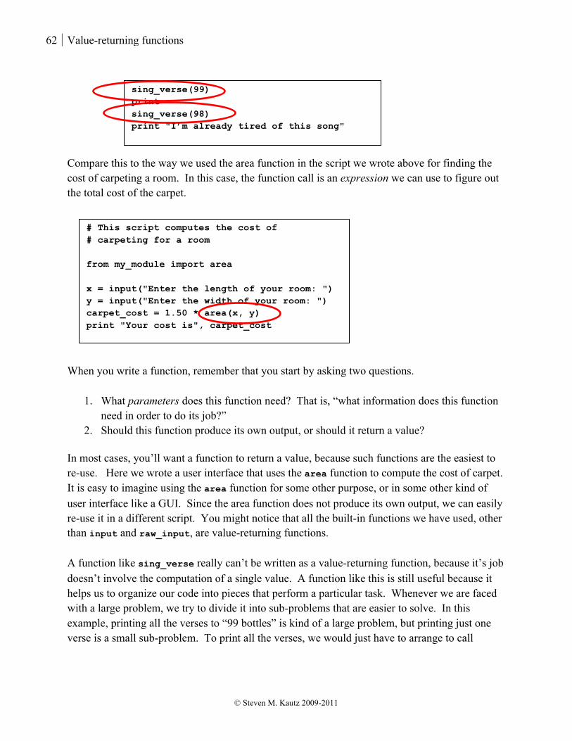
62 Value-returning functions
© Steven M. Kautz 2009-2011
Compare this to the way we used the area function in the script we wrote above for finding the cost of carpeting a room. In this case, the function call is an expression we can use to figure out the total cost of the carpet. When you write a function, remember that you start by asking two questions.
1. What parameters does this function need? That is, “what information does this function need in order to do its job?”
2. Should this function produce its own output, or should it return a value? In most cases, you’ll want a function to return a value, because such functions are the easiest to re-use. Here we wrote a user interface that uses the area function to compute the cost of carpet. It is easy to imagine using the area function for some other purpose, or in some other kind of user interface like a GUI. Since the area function does not produce its own output, we can easily re-use it in a different script. You might notice that all the built-in functions we have used, other than input and raw_input, are value-returning functions. A function like sing_verse really can’t be written as a value-returning function, because it’s job doesn’t involve the computation of a single value. A function like this is still useful because it helps us to organize our code into pieces that perform a particular task. Whenever we are faced with a large problem, we try to divide it into sub-problems that are easier to solve. In this example, printing all the verses to “99 bottles” is kind of a large problem, but printing just one verse is a small sub-problem. To print all the verses, we would just have to arrange to call
sing_verse(99) print sing_verse(98) print "I’m already tired of this song"
# This script computes the cost of # carpeting for a room from my_module import area x = input("Enter the length of your room: ") y = input("Enter the width of your room: ") carpet_cost = 1.50 * area(x, y) print "Your cost is", carpet_cost
There are eels in my hovercraft! 63
© Steven M. Kautz 2009-2011
sing_verse for each number between 99 and 0. As a peek ahead, we’ll see in a later chapter that we can do this very easily using something called a “for-loop”: for bottles in range(99, 0, -1): sing_verse(bottles)
It might be hard to see the point of writing a function like area, when it is so easy to calculate the value directly as the length times the width. But really, it only seems that way because we are just starting out. We’re writing scripts and functions that are just a few lines long. Once they start to get even a little bit more complex, we’ll appreciate the fact that we can write the code once inside a function and re-use it multiple times. Modern software systems involve hundreds of thousands of lines of code, and without the ability to divide them in modular pieces like functions, it would literally be impossible for them to be written at all!

64 Boolean operators and more about the return statement
© Steven M. Kautz 2009-2011
9. Boolean operators and more about the return statement
This section introduces the boolean operators represented by the Python keywords and, or, and not. Boolean operators enable us to simplify the logic of conditional statements by combining boolean expressions.
9.1. You will meet a tall and dark or not ugly and rich stranger
Let’s start by looking at an example that we used in a previous unit: Mousetraps are sold online for 2.00 each plus .50 for shipping, with free shipping for orders of 30 or more. The logic that we used to calculate the shipping could be expressed like this (where num refers to the number ordered): if num >= 30: shipping_cost = 0 else: shipping_cost = num * .50
Now suppose that shipping is also free for customers in zip code 50011. So before computing the shipping cost, we have to check the zip code. Assume that zip_code is a variable representing the zip code. if num >= 30: shipping_cost = 0 else: if zip_code == 50010: shipping_cost = 0 else: shipping_cost = num * .50
This makes sense, but doesn’t it seem a bit strange that the line shipping_cost = 0 appears in two places? if num >= 30: shipping_cost = 0 else: if zip_code == 50010: shipping_cost = 0 else: shipping_cost = num * .50
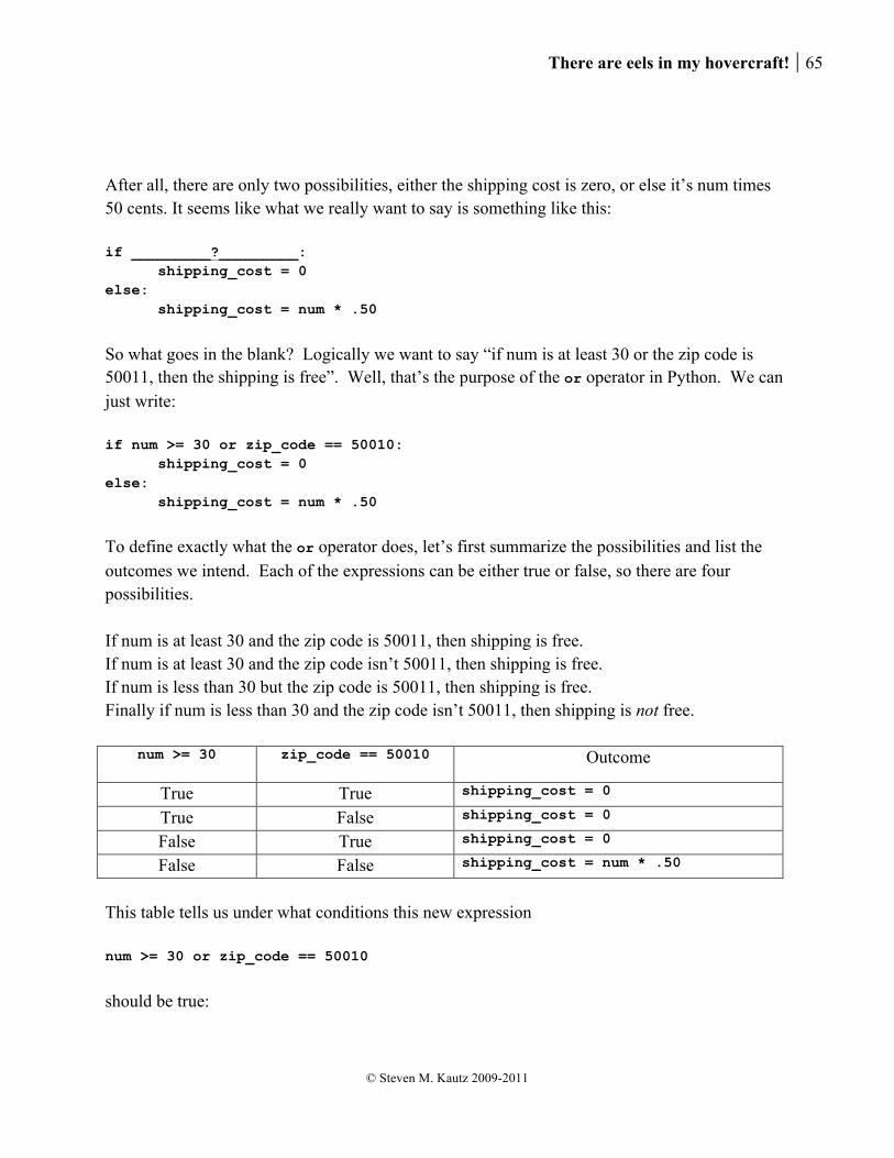
There are eels in my hovercraft! 65
© Steven M. Kautz 2009-2011
After all, there are only two possibilities, either the shipping cost is zero, or else it’s num times 50 cents. It seems like what we really want to say is something like this: if _________?_________: shipping_cost = 0 else: shipping_cost = num * .50
So what goes in the blank? Logically we want to say “if num is at least 30 or the zip code is 50011, then the shipping is free”. Well, that’s the purpose of the or operator in Python. We can just write: if num >= 30 or zip_code == 50010: shipping_cost = 0 else: shipping_cost = num * .50
To define exactly what the or operator does, let’s first summarize the possibilities and list the outcomes we intend. Each of the expressions can be either true or false, so there are four possibilities. If num is at least 30 and the zip code is 50011, then shipping is free. If num is at least 30 and the zip code isn’t 50011, then shipping is free. If num is less than 30 but the zip code is 50011, then shipping is free. Finally if num is less than 30 and the zip code isn’t 50011, then shipping is not free.
num >= 30 zip_code == 50010 Outcome
True True shipping_cost = 0 True False shipping_cost = 0 False True shipping_cost = 0 False False shipping_cost = num * .50
This table tells us under what conditions this new expression num >= 30 or zip_code == 50010 should be true:

66 Boolean operators and more about the return statement
© Steven M. Kautz 2009-2011
num >= 30 zip_code == 50010 num >= 30 or zip_code == 50010
True True True True False True False True True False False False
In fact, we can use the same table to define the or operator for any boolean expressions A and B.
A B A or B True True True True False True False True True False False False
The table tells us that the new expression A or B is true if at least one or A or B is true. This is called the truth table for the or operator. Let’s try another example. Suppose we have a function print_grade that prints the grade for a given score, but we first have to check that the score is between 0 and 100. We could write something like this: if score >= 0: if score <= 100: print_grade(score) else: print "out of range" else: print "out of range"
But again, it seems odd to have the same print statement appearing in two places. There are really only two possible outcomes, so we should be able to write something like this: if _________?_________: print_grade(score) else: print "out of range"
Now, what goes in the blank? We are trying to say “If score is above zero and less than 100, then print the grade.” That’s the purpose of the and keyword in Python.
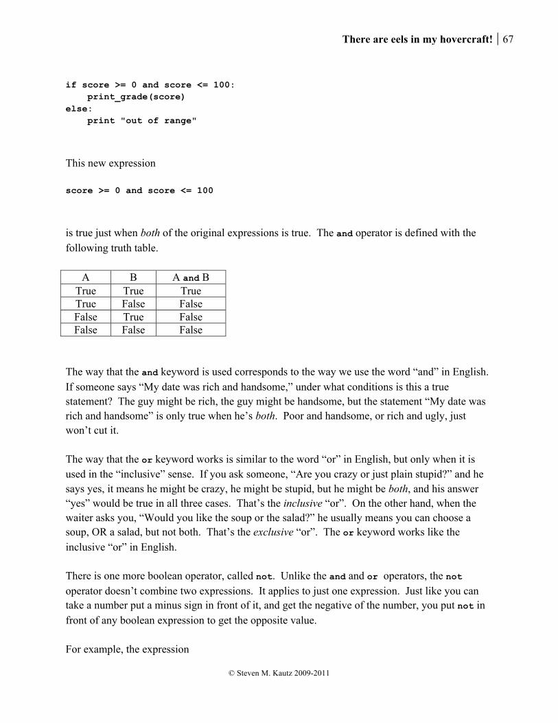
There are eels in my hovercraft! 67
© Steven M. Kautz 2009-2011
if score >= 0 and score <= 100: print_grade(score) else: print "out of range"
This new expression score >= 0 and score <= 100 is true just when both of the original expressions is true. The and operator is defined with the following truth table.
A B A and B True True True True False False False True False False False False
The way that the and keyword is used corresponds to the way we use the word “and” in English. If someone says “My date was rich and handsome,” under what conditions is this a true statement? The guy might be rich, the guy might be handsome, but the statement “My date was rich and handsome” is only true when he’s both. Poor and handsome, or rich and ugly, just won’t cut it. The way that the or keyword works is similar to the word “or” in English, but only when it is used in the “inclusive” sense. If you ask someone, “Are you crazy or just plain stupid?” and he says yes, it means he might be crazy, he might be stupid, but he might be both, and his answer “yes” would be true in all three cases. That’s the inclusive “or”. On the other hand, when the waiter asks you, “Would you like the soup or the salad?” he usually means you can choose a soup, OR a salad, but not both. That’s the exclusive “or”. The or keyword works like the inclusive “or” in English. There is one more boolean operator, called not. Unlike the and and or operators, the not operator doesn’t combine two expressions. It applies to just one expression. Just like you can take a number put a minus sign in front of it, and get the negative of the number, you put not in front of any boolean expression to get the opposite value. For example, the expression
68 Boolean operators and more about the return statement
© Steven M. Kautz 2009-2011
not(x > 0)
has the same meaning as x <= 0
Likewise, the expression not(x == 100)
means the same thing as x != 100
What about something like this? not(score >= 0 and score <= 100) You can read this as, “it is not the case that score is between 0 and 100”, which is the same as saying the score is less than 0 or is greater than 100: score < 0 or score > 100
(picture on number line). In all these examples, it was easy to rewrite the expression so that it doesn’t use the not operator. In some cases it is not so simple. Here is an example in which the not operator is extremely useful. We previously wrote a function is_divisible(a, b) that returns True when a is divisible by b and False otherwise. What if, given two values x and y, we want to say, “x is not divisible by y?” Well, one idea is to write a new function, but that is not always practical. But it is easy to simply write the expression not is_divisible(x, y) which has value True exactly when is_divisible(x, y) has value False. The operators or, and, and not can be repeated or combined. For example, you could say “x is equal to 3, 5, or 7” using the expression x == 3 or x == 5 or x == 7
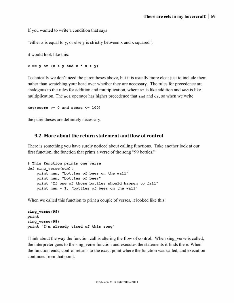
There are eels in my hovercraft! 69
© Steven M. Kautz 2009-2011
If you wanted to write a condition that says “either x is equal to y, or else y is strictly between x and x squared”, it would look like this: x == y or (x < y and x * x > y)
Technically we don’t need the parentheses above, but it is usually more clear just to include them rather than scratching your head over whether they are necessary. The rules for precedence are analogous to the rules for addition and multiplication, where or is like addition and and is like multiplication. The not operator has higher precedence that and and or, so when we write not(score >= 0 and score <= 100) the parentheses are definitely necessary.
9.2. More about the return statement and flow of control
There is something you have surely noticed about calling functions. Take another look at our first function, the function that prints a verse of the song “99 bottles.” # This function prints one verse def sing_verse(num): print num, "bottles of beer on the wall" print num, "bottles of beer" print "If one of those bottles should happen to fall" print num - 1, "bottles of beer on the wall"
When we called this function to print a couple of verses, it looked like this: sing_verse(99) print sing_verse(98) print "I’m already tired of this song"
Think about the way the function call is altering the flow of control. When sing_verse is called, the interpreter goes to the sing_verse function and executes the statements it finds there. When the function ends, control returns to the exact point where the function was called, and execution continues from that point.
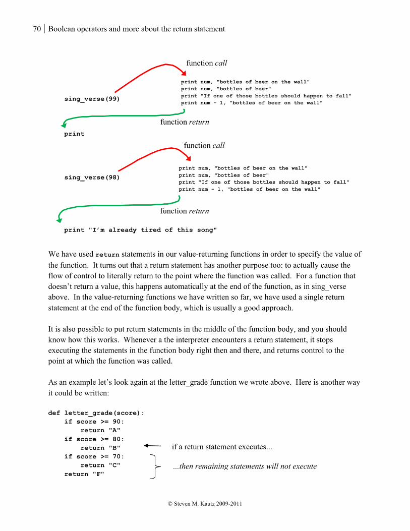
70 Boolean operators and more about the return statement
© Steven M. Kautz 2009-2011
We have used return statements in our value-returning functions in order to specify the value of the function. It turns out that a return statement has another purpose too: to actually cause the flow of control to literally return to the point where the function was called. For a function that doesn’t return a value, this happens automatically at the end of the function, as in sing_verse above. In the value-returning functions we have written so far, we have used a single return statement at the end of the function body, which is usually a good approach. It is also possible to put return statements in the middle of the function body, and you should know how this works. Whenever a the interpreter encounters a return statement, it stops executing the statements in the function body right then and there, and returns control to the point at which the function was called. As an example let’s look again at the letter_grade function we wrote above. Here is another way it could be written: def letter_grade(score): if score >= 90: return "A" if score >= 80: return "B" if score >= 70: return "C" return "F"
sing_verse(99) print sing_verse(98) print "I’m already tired of this song"
print num, "bottles of beer on the wall" print num, "bottles of beer" print "If one of those bottles should happen to fall" print num - 1, "bottles of beer on the wall"
print num, "bottles of beer on the wall" print num, "bottles of beer" print "If one of those bottles should happen to fall" print num - 1, "bottles of beer on the wall"
function call
function call
function return
function return
...then remaining statements will not execute
if a return statement executes...
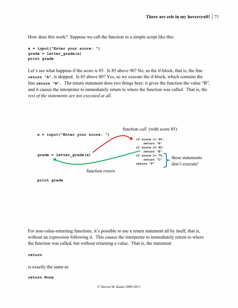
There are eels in my hovercraft! 71
© Steven M. Kautz 2009-2011
How does this work? Suppose we call the function in a simple script like this: x = input("Enter your score: ") grade = letter_grade(x) print grade
Let’s see what happens if the score is 85. Is 85 above 90? No, so the if-block, that is, the line return "A", is skipped. Is 85 above 80? Yes, so we execute the if-block, which contains the line return "B". The return statement does two things here: it gives the function the value “B”, and it causes the interpreter to immediately return to where the function was called. That is, the rest of the statements are not executed at all.
For non-value-returning functions, it’s possible to use a return statement all by itself, that is, without an expression following it. This causes the interpreter to immediately return to where the function was called, but without returning a value. That is, the statement return
is exactly the same as return None
x = input("Enter your score: ") grade = letter_grade(x) print grade
if score >= 90: return "A" if score >= 80: return "B" if score >= 70: return "C" return "F"
function call (with score 85)
function return
these statements don’t execute!
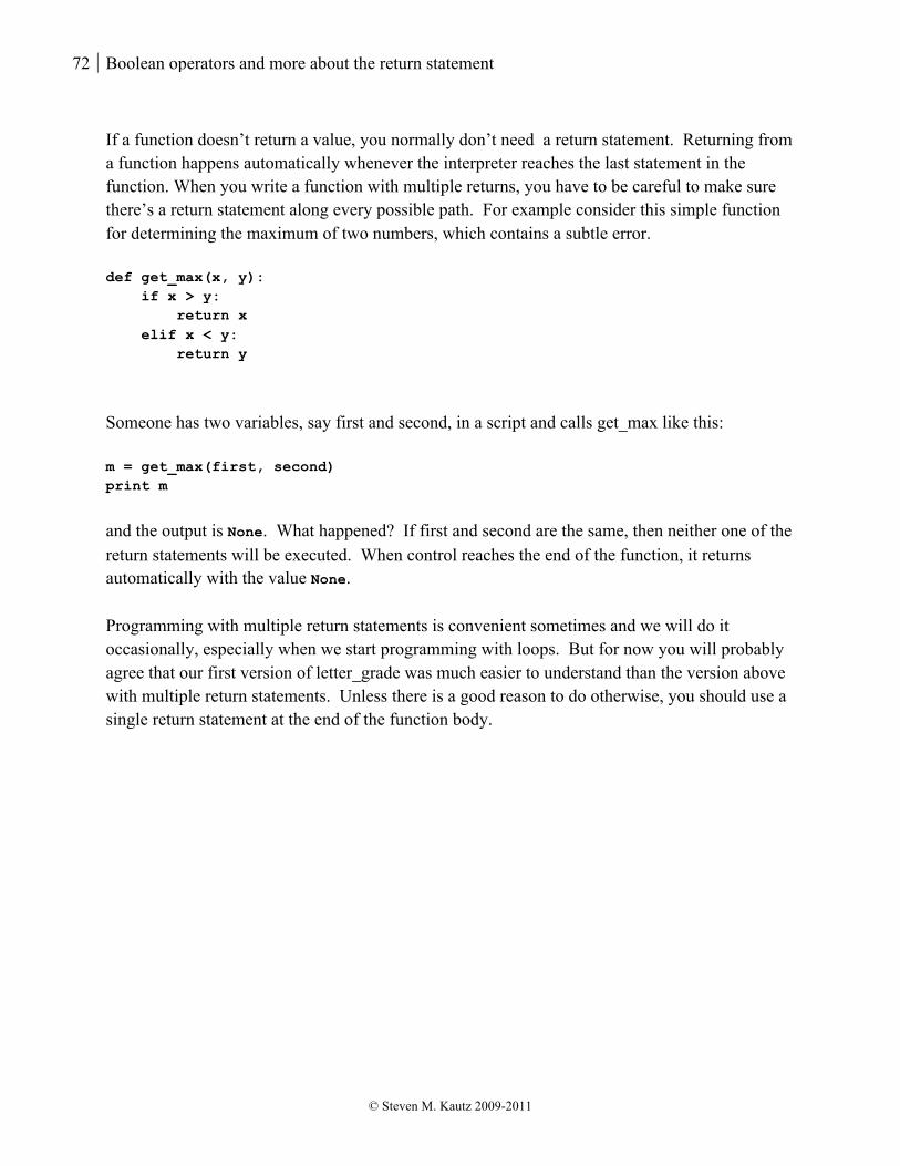
72 Boolean operators and more about the return statement
© Steven M. Kautz 2009-2011
If a function doesn’t return a value, you normally don’t need a return statement. Returning from a function happens automatically whenever the interpreter reaches the last statement in the function. When you write a function with multiple returns, you have to be careful to make sure there’s a return statement along every possible path. For example consider this simple function for determining the maximum of two numbers, which contains a subtle error. def get_max(x, y): if x > y: return x elif x < y: return y
Someone has two variables, say first and second, in a script and calls get_max like this: m = get_max(first, second) print m
and the output is None. What happened? If first and second are the same, then neither one of the return statements will be executed. When control reaches the end of the function, it returns automatically with the value None. Programming with multiple return statements is convenient sometimes and we will do it occasionally, especially when we start programming with loops. But for now you will probably agree that our first version of letter_grade was much easier to understand than the version above with multiple return statements. Unless there is a good reason to do otherwise, you should use a single return statement at the end of the function body.

There are eels in my hovercraft! 73
© Steven M. Kautz 2009-2011
10. Unit testing and incremental development
As we start to write programs that are more complex and use multiple modules, we will find we won’t be able to have a complete solution in our minds before we start writing it. We need some techniques to develop a system incrementally, that is, a little bit at a time. In this chapter we introduce the idea of a unit test as a way to guide the development of a function and check whether it is working correctly.
10.1. An example, and an introduction to unit testing
Suppose that donuts are .75 each or 8.00 per dozen, and coffee is 1.50. But you get two free coffees for each full dozen donuts you buy. Write a function called coffee_break that returns the total cost for a given number of donuts and coffees. We can see that two parameters are required: the number of donuts purchased, and the number of coffees purchased, so we know the function definition will look like this: def coffee_break (num_donuts, num_coffees):
As always, let’s start with some concrete examples. We can look at some simple cases first that don’t involve coffee. How much for 4 donuts? That’s not a full dozen, so they’re just .75 each. 4 * .75 is 3.00. How much for 16 donuts? There’s 1 dozen, and 4 single donuts. It’s 8.00 for the dozen 4 * .75 is 3.00 for 4 singles 8.00 + 3.00 is 11.00 total How about 100 donuts? Hmm. We need to know how many dozen there are in 100. Well, that’s just 100 divided by 12, which is 8. And of course the number of single donuts is just the remainder, which is 4.

74 Unit testing and incremental development
© Steven M. Kautz 2009-2011
8 * 8.00 is 64.00 for 8 dozen 4 * .75 is 3.00 for 4 singles 64.00 + 3.00 is 67.00 total Those were pretty easy. Let’s see what happens when we start buying coffee too. How much for 4 donuts and 4 coffees? Well, we figured out before that 4 donuts is 3.00 4 * 1.50 is 6.00 for 4 coffees 3.00 + 6.00 is 9.00 total How about 16 donuts and 4 coffees? We already discovered that the cost of the 16 donuts is 11.00 But since we’re buying a full dozen donuts, we get 2 free coffees. That means we only have to pay for two coffees. 2 * 1.50 is 3.00 11.00 + 3.00 = 14.00 total How about 100 donuts and 4 coffees? We know that 100 donuts cost 67.00 But we’re buying 8 dozen, so we get 16 free coffees. Therefore our four coffees are all free. 67.00 is the total. So we now have six “test cases” – sample values for which we know what the result should be, so we’re ready to start writing the function. After we write it, we’ll want to check whether we’re getting the right answers for our test cases. How would we check? We might write a simple script like this one that just prints the results from each function call: print coffee_break (4, 0) print coffee_break (16, 0) print coffee_break (100, 0) print coffee_break (4, 4) print coffee_break (16, 4) print coffee_break (100, 4)
When we run this script, what we hope to see are the answers we computed by hand: 3.00 11.00 67.00 9.00 14.00 67.00
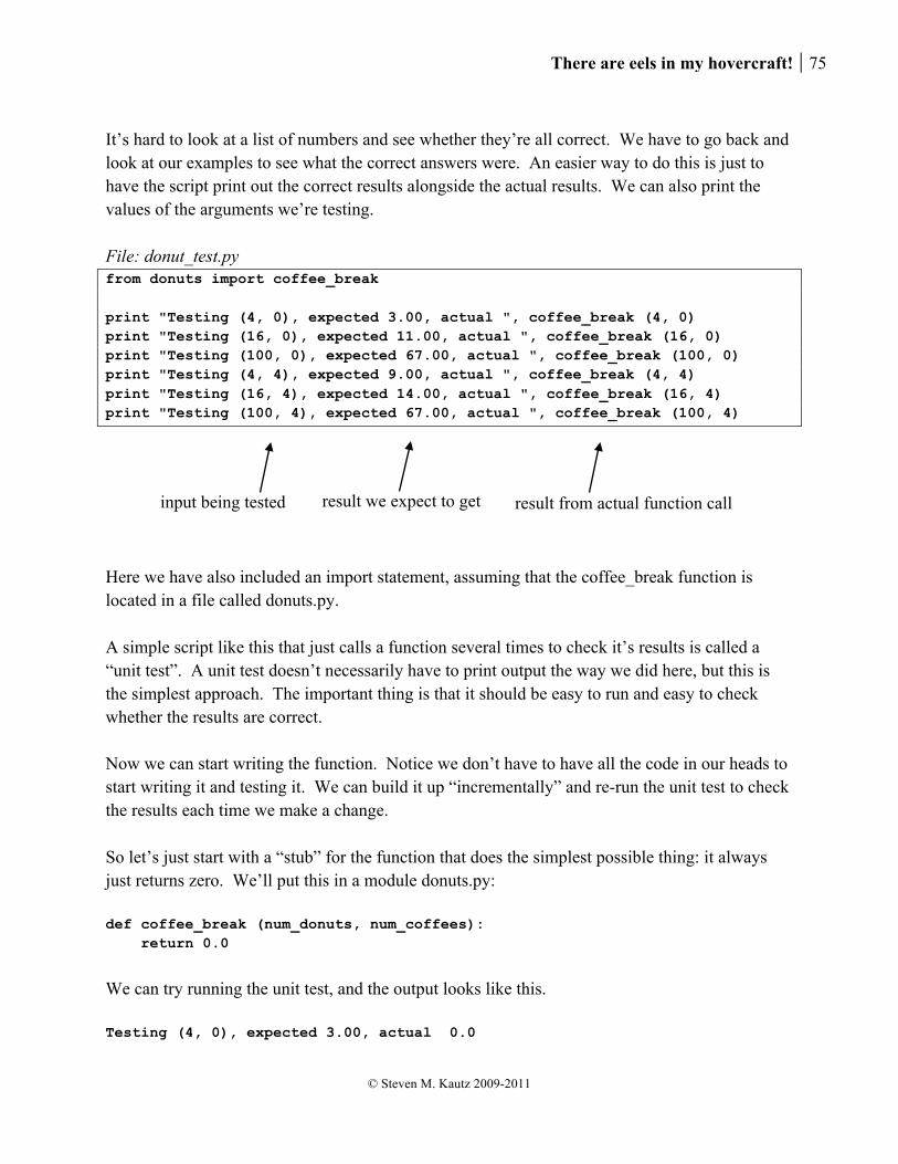
There are eels in my hovercraft! 75
© Steven M. Kautz 2009-2011
It’s hard to look at a list of numbers and see whether they’re all correct. We have to go back and look at our examples to see what the correct answers were. An easier way to do this is just to have the script print out the correct results alongside the actual results. We can also print the values of the arguments we’re testing. File: donut_test.py from donuts import coffee_break print "Testing (4, 0), expected 3.00, actual ", coffee_break (4, 0) print "Testing (16, 0), expected 11.00, actual ", coffee_break (16, 0) print "Testing (100, 0), expected 67.00, actual ", coffee_break (100, 0) print "Testing (4, 4), expected 9.00, actual ", coffee_break (4, 4) print "Testing (16, 4), expected 14.00, actual ", coffee_break (16, 4) print "Testing (100, 4), expected 67.00, actual ", coffee_break (100, 4)
Here we have also included an import statement, assuming that the coffee_break function is located in a file called donuts.py. A simple script like this that just calls a function several times to check it’s results is called a “unit test”. A unit test doesn’t necessarily have to print output the way we did here, but this is the simplest approach. The important thing is that it should be easy to run and easy to check whether the results are correct. Now we can start writing the function. Notice we don’t have to have all the code in our heads to start writing it and testing it. We can build it up “incrementally” and re-run the unit test to check the results each time we make a change. So let’s just start with a “stub” for the function that does the simplest possible thing: it always just returns zero. We’ll put this in a module donuts.py: def coffee_break (num_donuts, num_coffees): return 0.0
We can try running the unit test, and the output looks like this. Testing (4, 0), expected 3.00, actual 0.0
input being tested result we expect to get result from actual function call
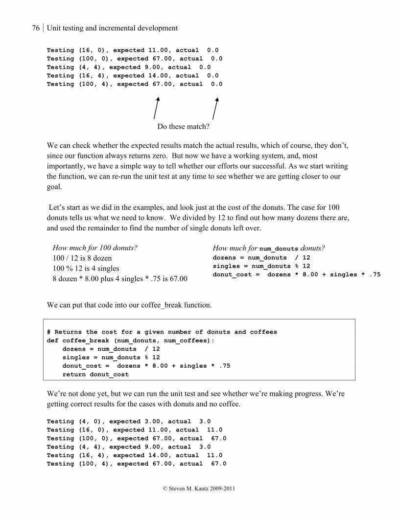
76 Unit testing and incremental development
© Steven M. Kautz 2009-2011
Testing (16, 0), expected 11.00, actual 0.0 Testing (100, 0), expected 67.00, actual 0.0 Testing (4, 4), expected 9.00, actual 0.0 Testing (16, 4), expected 14.00, actual 0.0 Testing (100, 4), expected 67.00, actual 0.0
We can check whether the expected results match the actual results, which of course, they don’t, since our function always returns zero. But now we have a working system, and, most importantly, we have a simple way to tell whether our efforts our successful. As we start writing the function, we can re-run the unit test at any time to see whether we are getting closer to our goal. Let’s start as we did in the examples, and look just at the cost of the donuts. The case for 100 donuts tells us what we need to know. We divided by 12 to find out how many dozens there are, and used the remainder to find the number of single donuts left over.
We can put that code into our coffee_break function. # Returns the cost for a given number of donuts and coffees def coffee_break (num_donuts, num_coffees): dozens = num_donuts / 12 singles = num_donuts % 12 donut_cost = dozens * 8.00 + singles * .75 return donut_cost
We’re not done yet, but we can run the unit test and see whether we’re making progress. We’re getting correct results for the cases with donuts and no coffee. Testing (4, 0), expected 3.00, actual 3.0 Testing (16, 0), expected 11.00, actual 11.0 Testing (100, 0), expected 67.00, actual 67.0 Testing (4, 4), expected 9.00, actual 3.0 Testing (16, 4), expected 14.00, actual 11.0 Testing (100, 4), expected 67.00, actual 67.0
Do these match?
How much for 100 donuts? 100 / 12 is 8 dozen 100 % 12 is 4 singles 8 dozen * 8.00 plus 4 singles * .75 is 67.00
How much for num_donuts donuts? dozens = num_donuts / 12 singles = num_donuts % 12 donut_cost = dozens * 8.00 + singles * .75
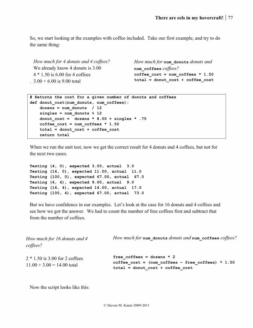
There are eels in my hovercraft! 77
© Steven M. Kautz 2009-2011
So, we start looking at the examples with coffee included. Take our first example, and try to do the same thing: We can add the coffee cost into the function. # Returns the cost for a given number of donuts and coffees def donut_cost(num_donuts, num_coffees): dozens = num_donuts / 12 singles = num_donuts % 12 donut_cost = dozens * 8.00 + singles * .75 coffee_cost = num_coffees * 1.50 total = donut_cost + coffee_cost return total
When we run the unit test, now we get the correct result for 4 donuts and 4 coffees, but not for the next two cases. Testing (4, 0), expected 3.00, actual 3.0 Testing (16, 0), expected 11.00, actual 11.0 Testing (100, 0), expected 67.00, actual 67.0 Testing (4, 4), expected 9.00, actual 9.0 Testing (16, 4), expected 14.00, actual 17.0 Testing (100, 4), expected 67.00, actual 73.0
But we have confidence in our examples. Let’s look at the case for 16 donuts and 4 coffees and see how we got the answer. We had to count the number of free coffees first and subtract that from the number of coffees.
Now the script looks like this:
How much for 4 donuts and 4 coffees? We already know 4 donuts is 3.00 4 * 1.50 is 6.00 for 4 coffees 3.00 + 6.00 is 9.00 total
How much for num_donuts donuts and num_coffees coffees? coffee_cost = num_coffees * 1.50 total = donut_cost + coffee_cost
How much for 16 donuts and 4 coffees? 2 * 1.50 is 3.00 for 2 coffees 11.00 + 3.00 = 14.00 total
How much for num_donuts donuts and num_coffees coffees? free_coffees = dozens * 2 coffee_cost = (num_coffees – free_coffees) * 1.50 total = donut_cost + coffee_cost
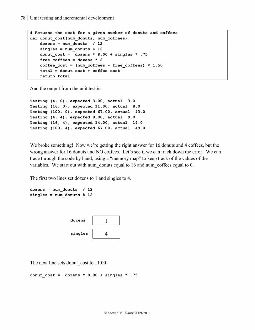
78 Unit testing and incremental development
© Steven M. Kautz 2009-2011
# Returns the cost for a given number of donuts and coffees def donut_cost(num_donuts, num_coffees): dozens = num_donuts / 12 singles = num_donuts % 12 donut_cost = dozens * 8.00 + singles * .75 free_coffees = dozens * 2 coffee_cost = (num_coffees - free_coffees) * 1.50 total = donut_cost + coffee_cost return total
And the output from the unit test is: Testing (4, 0), expected 3.00, actual 3.0 Testing (16, 0), expected 11.00, actual 8.0 Testing (100, 0), expected 67.00, actual 43.0 Testing (4, 4), expected 9.00, actual 9.0 Testing (16, 4), expected 14.00, actual 14.0 Testing (100, 4), expected 67.00, actual 49.0
We broke something! Now we’re getting the right answer for 16 donuts and 4 coffees, but the wrong answer for 16 donuts and NO coffees. Let’s see if we can track down the error. We can trace through the code by hand, using a “memory map” to keep track of the values of the variables. We start out with num_donuts equal to 16 and num_coffees equal to 0. The first two lines set dozens to 1 and singles to 4. dozens = num_donuts / 12 singles = num_donuts % 12
The next line sets donut_cost to 11.00. donut_cost = dozens * 8.00 + singles * .75
1 dozens
4 singles
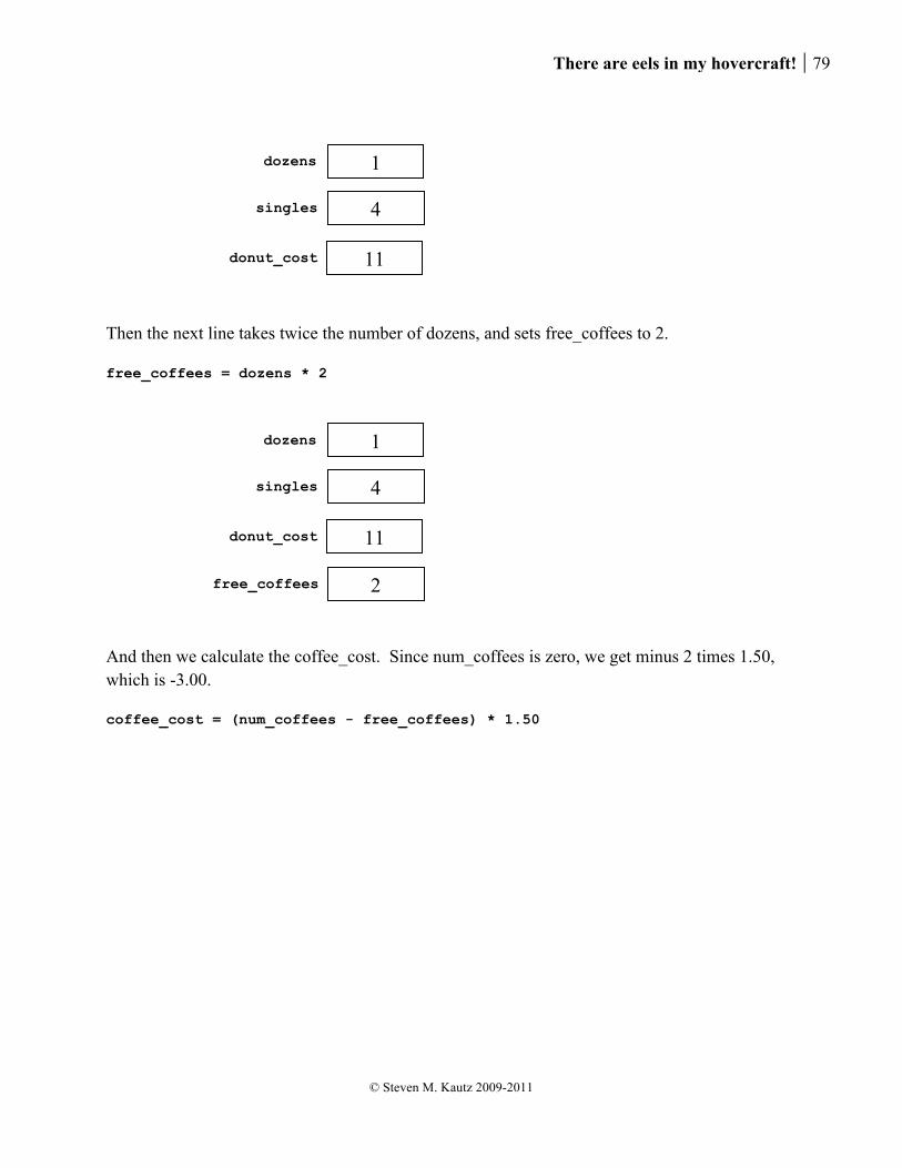
There are eels in my hovercraft! 79
© Steven M. Kautz 2009-2011
Then the next line takes twice the number of dozens, and sets free_coffees to 2. free_coffees = dozens * 2
And then we calculate the coffee_cost. Since num_coffees is zero, we get minus 2 times 1.50, which is -3.00. coffee_cost = (num_coffees - free_coffees) * 1.50
1 dozens
4 singles
11 donut_cost
1 dozens
4 singles
11 donut_cost
2 free_coffees

80 Unit testing and incremental development
© Steven M. Kautz 2009-2011
Wait a minute! That can’t be right. The coffee cost should be zero, since we aren’t ordering any coffees. That’s where the error is. We only want to compute the coffee_cost this way if the number of coffees ordered is greater than, or equal to, the number of free coffees. We can just replace that line with a conditional statement: if num_coffees >= free_coffees: coffee_cost = (num_coffees - free_coffees) * 1.50 else: coffee_cost = 0
Now when we re-run the unit test, all the results are all correct.
10.2. Another example
Here is an example of a function that uses the boolean operators from the last chapter In the calendar used in western countries, some years have 366 days instead of 365. These are called “leap years.” A year is defined to be a leap year if it is divisible by 400, or if it is divisible by 4 but not by 100. Write a function called is_leap_year that returns True if a given year is a leap year, and False otherwise. The definition is a little bit confusing to most of us. We’d better start with some examples.
1 dozens
4 singles
11.00 donut_cost
2 free_coffees
-3.00 coffee_cost
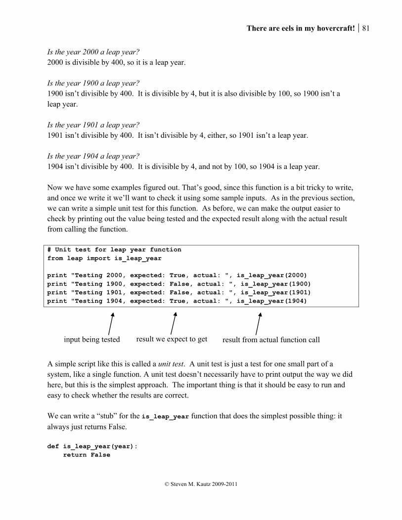
There are eels in my hovercraft! 81
© Steven M. Kautz 2009-2011
Is the year 2000 a leap year? 2000 is divisible by 400, so it is a leap year. Is the year 1900 a leap year? 1900 isn’t divisible by 400. It is divisible by 4, but it is also divisible by 100, so 1900 isn’t a leap year. Is the year 1901 a leap year? 1901 isn’t divisible by 400. It isn’t divisible by 4, either, so 1901 isn’t a leap year. Is the year 1904 a leap year? 1904 isn’t divisible by 400. It is divisible by 4, and not by 100, so 1904 is a leap year. Now we have some examples figured out. That’s good, since this function is a bit tricky to write, and once we write it we’ll want to check it using some sample inputs. As in the previous section, we can write a simple unit test for this function. As before, we can make the output easier to check by printing out the value being tested and the expected result along with the actual result from calling the function. # Unit test for leap year function from leap import is_leap_year print "Testing 2000, expected: True, actual: ", is_leap_year(2000) print "Testing 1900, expected: False, actual: ", is_leap_year(1900) print "Testing 1901, expected: False, actual: ", is_leap_year(1901) print "Testing 1904, expected: True, actual: ", is_leap_year(1904)
A simple script like this is called a unit test. A unit test is just a test for one small part of a system, like a single function. A unit test doesn’t necessarily have to print output the way we did here, but this is the simplest approach. The important thing is that it should be easy to run and easy to check whether the results are correct. We can write a “stub” for the is_leap_year function that does the simplest possible thing: it always just returns False. def is_leap_year(year): return False
input being tested result we expect to get result from actual function call
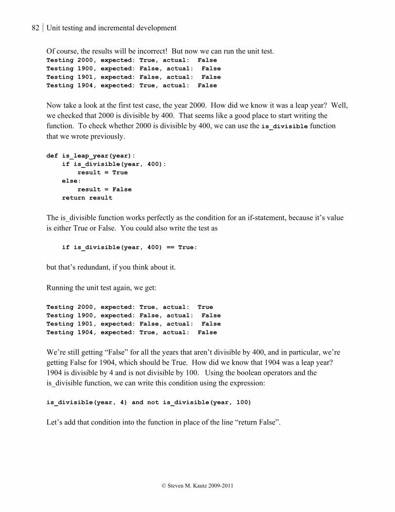
82 Unit testing and incremental development
© Steven M. Kautz 2009-2011
Of course, the results will be incorrect! But now we can run the unit test. Testing 2000, expected: True, actual: False Testing 1900, expected: False, actual: False Testing 1901, expected: False, actual: False Testing 1904, expected: True, actual: False
Now take a look at the first test case, the year 2000. How did we know it was a leap year? Well, we checked that 2000 is divisible by 400. That seems like a good place to start writing the function. To check whether 2000 is divisible by 400, we can use the is_divisible function that we wrote previously. def is_leap_year(year): if is_divisible(year, 400): result = True else: result = False return result
The is_divisible function works perfectly as the condition for an if-statement, because it’s value is either True or False. You could also write the test as if is_divisible(year, 400) == True:
but that’s redundant, if you think about it. Running the unit test again, we get: Testing 2000, expected: True, actual: True Testing 1900, expected: False, actual: False Testing 1901, expected: False, actual: False Testing 1904, expected: True, actual: False
We’re still getting “False” for all the years that aren’t divisible by 400, and in particular, we’re getting False for 1904, which should be True. How did we know that 1904 was a leap year? 1904 is divisible by 4 and is not divisible by 100. Using the boolean operators and the is_divisible function, we can write this condition using the expression: is_divisible(year, 4) and not is_divisible(year, 100) Let’s add that condition into the function in place of the line “return False”.

There are eels in my hovercraft! 83
© Steven M. Kautz 2009-2011
def is_leap_year(year): if is_divisible(year, 400): result = True else: if is_divisible(year, 4) and not is_divisible(year, 100): result = True else: result = False return result
Re-running the unit tests shows that we now get correct results in all cases. Testing 2000, expected: True, actual: True Testing 1900, expected: False, actual: False Testing 1901, expected: False, actual: False Testing 1904, expected: True, actual: True
You may notice that the function can be simplified a bit more, since we’re setting the result to True in two different places. We can combine the two conditional tests using the or operator: def is_leap_year(year): if is_divisible(year, 400) or is_divisible(year, 4) and not is_divisible(year, 100): result = True else: result = False return result
Or even: def is_leap_year(year): return is_divisible(year, 400) or (is_divisible(year, 4) and not is_divisible(year, 100))
Does it still work? Easy enough to check; just re-run the unit test! Long lines, like the condition in the if-statement above, can get hard to read. Python allows us to break up long lines by adding a backslash character at the end of a line to indicate “to be continued”. A more legible version of the function would be written like this: def is_leap_year(year): if is_divisible(year, 400) or \ is_divisible(year, 4) and not is_divisible(year, 100): result = True else: result = False return result

84 Bugs!
© Steven M. Kautz 2009-2011
11. Bugs! No doubt you have already discovered that when you sit down to write a program, you generally don’t get it right the first time. There are several kinds of things that might go wrong.
• Syntax errors – the interpreter can’t run your code at all because it doesn’t completely conform to the grammar of the Python language. You get syntax errors from missing colons, extra whitespace, misspelled keywords, and things like that
• Runtime errors – your code runs, but an error occurs when you run it. Examples include division by zero, missing modules, or trying to add an int to a string.
• Logic errors – your code runs fine and gives you results, but the results are incorrect. In general, any kind of error in a program is called a “bug”. The process of finding and fixing the errors is called “debugging”. Debugging can be extremely challenging, but is a necessary part of the process of programming. Sometimes you will need to use all the ingenuity and creativity you can muster!
11.1. Finding syntax errors
Syntax errors are usually the easiest to find, because the interpreter will always tell you where it got stuck trying to figure out the structure of your code. However, you have probably noticed that the error messages don’t always correspond exactly to where the error really is! Let’s start with an example to illustrate some common errors and how to find them. Here is a function that prints the solutions to a quadratic equation. It contains a number of errors. from math import sqrt
# Prints the solutions to a quadratic equation # Warning: this code has bugs! def print_solutions(a, b, c): temp == b * b - 4 * a * c if temp == 0 solution = -b / 2(a) print "There is one solution: ", solution else if temp < 0: print "There are no solutions else: solution1 = (-b + sqrt(temp) / (2 * a)
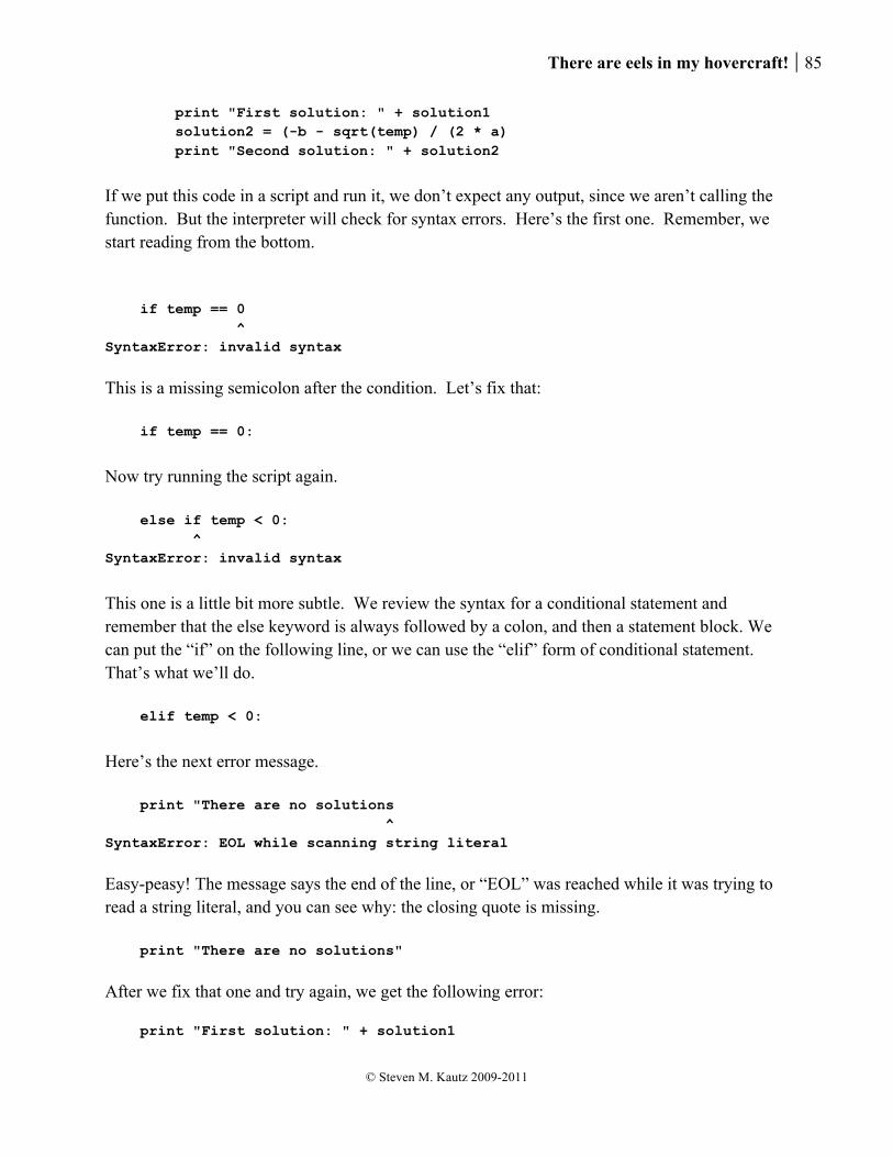
There are eels in my hovercraft! 85
© Steven M. Kautz 2009-2011
print "First solution: " + solution1 solution2 = (-b - sqrt(temp) / (2 * a) print "Second solution: " + solution2 If we put this code in a script and run it, we don’t expect any output, since we aren’t calling the function. But the interpreter will check for syntax errors. Here’s the first one. Remember, we start reading from the bottom. if temp == 0 ^ SyntaxError: invalid syntax
This is a missing semicolon after the condition. Let’s fix that: if temp == 0:
Now try running the script again. else if temp < 0: ^ SyntaxError: invalid syntax
This one is a little bit more subtle. We review the syntax for a conditional statement and remember that the else keyword is always followed by a colon, and then a statement block. We can put the “if” on the following line, or we can use the “elif” form of conditional statement. That’s what we’ll do. elif temp < 0:
Here’s the next error message. print "There are no solutions ^ SyntaxError: EOL while scanning string literal
Easy-peasy! The message says the end of the line, or “EOL” was reached while it was trying to read a string literal, and you can see why: the closing quote is missing. print "There are no solutions"
After we fix that one and try again, we get the following error: print "First solution: " + solution1
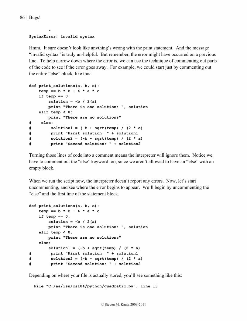
86 Bugs!
© Steven M. Kautz 2009-2011
^ SyntaxError: invalid syntax
Hmm. It sure doesn’t look like anything’s wrong with the print statement. And the message “invalid syntax” is truly un-helpful. But remember, the error might have occurred on a previous line. To help narrow down where the error is, we can use the technique of commenting out parts of the code to see if the error goes away. For example, we could start just by commenting out the entire “else” block, like this: def print_solutions(a, b, c): temp == b * b - 4 * a * c if temp == 0: solution = -b / 2(a) print "There is one solution: ", solution elif temp < 0: print "There are no solutions" # else: # solution1 = (-b + sqrt(temp) / (2 * a) # print "First solution: " + solution1 # solution2 = (-b - sqrt(temp) / (2 * a) # print "Second solution: " + solution2
Turning those lines of code into a comment means the interpreter will ignore them. Notice we have to comment out the “else” keyword too, since we aren’t allowed to have an “else” with an empty block. When we run the script now, the interpreter doesn’t report any errors. Now, let’s start uncommenting, and see where the error begins to appear. We’ll begin by uncommenting the “else” and the first line of the statement block. def print_solutions(a, b, c): temp == b * b - 4 * a * c if temp == 0: solution = -b / 2(a) print "There is one solution: ", solution elif temp < 0: print "There are no solutions" else: solution1 = (-b + sqrt(temp) / (2 * a) # print "First solution: " + solution1 # solution2 = (-b - sqrt(temp) / (2 * a) # print "Second solution: " + solution2
Depending on where your file is actually stored, you’ll see something like this: File "C:/aa/isu/cs104/python/quadratic.py", line 13
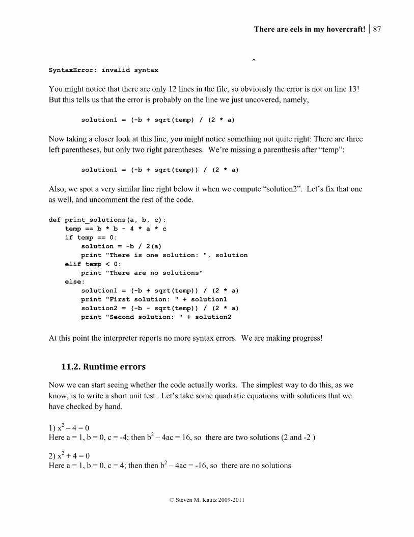
There are eels in my hovercraft! 87
© Steven M. Kautz 2009-2011
^ SyntaxError: invalid syntax
You might notice that there are only 12 lines in the file, so obviously the error is not on line 13! But this tells us that the error is probably on the line we just uncovered, namely, solution1 = (-b + sqrt(temp) / (2 * a)
Now taking a closer look at this line, you might notice something not quite right: There are three left parentheses, but only two right parentheses. We’re missing a parenthesis after “temp”: solution1 = (-b + sqrt(temp)) / (2 * a)
Also, we spot a very similar line right below it when we compute “solution2”. Let’s fix that one as well, and uncomment the rest of the code. def print_solutions(a, b, c): temp == b * b - 4 * a * c if temp == 0: solution = -b / 2(a) print "There is one solution: ", solution elif temp < 0: print "There are no solutions" else: solution1 = (-b + sqrt(temp)) / (2 * a) print "First solution: " + solution1 solution2 = (-b - sqrt(temp)) / (2 * a) print "Second solution: " + solution2
At this point the interpreter reports no more syntax errors. We are making progress!
11.2. Runtime errors
Now we can start seeing whether the code actually works. The simplest way to do this, as we know, is to write a short unit test. Let’s take some quadratic equations with solutions that we have checked by hand. 1) x2 – 4 = 0 Here a = 1, b = 0, c = -4; then b2 – 4ac = 16, so there are two solutions (2 and -2 ) 2) x2 + 4 = 0 Here a = 1, b = 0, c = 4; then then b2 – 4ac = -16, so there are no solutions

88 Bugs!
© Steven M. Kautz 2009-2011
3) 4x2 – 4x + 1 = 0 Here a = 4, b = -4, c = 1; then b2 – 4ac = 0, so there is one solution (1/2). 4) 2x2 – 9x – 5 = 0 Here a = 2, b = -9, c = -5; then b2 – 4ac = 121, so there are two solutions (5 and -1/2) We can put these examples together into a unit test that might look like this: from quadratic import print_solutions print "a = 1, b = 0, c = -4, expected two solutions 2 and -2:" print_solutions(1, 0, -4) print print "a = 1, b = 0, c = 4, expected no solutions:" print_solutions(1, 0, 4) print print "a = 4, b = -4, c = 1, expected one solution 0.5:" print_solutions(4, -4, 1) print print "a = 2, b = -9, c = -5, expected two solutions 5 and -0.5:" print_solutions(2, -9, -5)
Now we get a runtime error when we try to run the unit test. temp == b * b - 4 * a * c NameError: global name 'temp' is not defined
What? Aren’t we defining “temp” right in this line? Oh, wait a minute. That’s a double-equals, not an assignment statement. We fix it so it says: temp = b * b - 4 * a * c
Now run the unit test again. We get the error: print "First solution: " + solution1 TypeError: cannot concatenate 'str' and 'float' objects
Ok, we’ve seen that one before. We have to convert “solution1” to a string to concatenate. print "First solution: " + str(solution1)
The same error occurs one line down when we’re printing the second solution, so we fix that one too. Try again! solution = -b / 2(a)

There are eels in my hovercraft! 89
© Steven M. Kautz 2009-2011
TypeError: 'int' object is not callable
That is the most incomprehensible error message we’ve seen yet, isn’t it? Here’s what it means. Think about how we call functions: the function’s name, followed by a pair of parentheses. It turns out that the only situation where you can directly follow something with parentheses is when you’re calling a function. The interpreter is telling us that the number “2” is not a function that we can call. Remember, to multiply we have to actually use the “star” operator: solution = -b / (2 * a)
Now the unit test runs without errors.
11.3. Logic errors
The unit test runs without errors, but we’re not getting the correct results. a = 1, b = 0, c = -4, expected two solutions 2 and -2: First solution: 2.0 Second solution: -2.0 a = 1, b = 0, c = 4, expected no solutions: There are no solutions a = 4, b = -4, c = 1, expected one solution 0.5: There is one solution: 0 a = 2, b = -9, c = -5, expected two solutions 5 and -0.5: First solution: 5.0 Second solution: -0.5
The third case doesn’t seem to match the expected answer. We read the code again and it seems to be correct: if temp == 0: solution = -b / (2 * a) print "There is one solution: ", solution
That is, we are clearly entering the right block of code, since we’re getting the message “There is one solution”. And we can check the arithmetic with a calculator and it’s right. What we can do is to put some extra print statements into the code to see what’s going on. These extra print statements will be temporary, and we’ll remove them once we figure out what’s wrong. Here is an example. We’ll compute the numerator and denominator of –b/2a separately and print the values so we can see them.
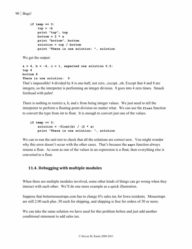
90 Bugs!
© Steven M. Kautz 2009-2011
if temp == 0: top = -b print "top", top bottom = 2 * a print "bottom", bottom solution = top / bottom print "There is one solution: ", solution
We get the output: a = 4, b = -4, c = 1, expected one solution 0.5: top 4 bottom 8 There is one solution: 0
That’s impossible! 4 divided by 8 is one-half, not zero...except...oh. Except that 4 and 8 are integers, so the interpreter is performing an integer division. 8 goes into 4 zero times. Smack forehead with palm! There is nothing to restrict a, b, and c from being integer values. We just need to tell the interpreter to perform a floating-point division no matter what. We can use the float function to convert the type from int to float. It is enough to convert just one of the values. if temp == 0: solution = -float(b) / (2 * a) print "There is one solution: ", solution
We can re-run the unit test to check that all the solutions are correct now. You might wonder why this error doesn’t occur with the other cases. That’s because the sqrt function always returns a float. As soon as one of the values in an expression is a float, then everything else is converted to a float.
11.4. Debugging with multiple modules
When there are multiple modules involved, some other kinds of things can go wrong when they interact with each other. We’ll do one more example as a quick illustration. Suppose that bettermousetraps.com has to charge 6% sales tax for Iowa residents. Mousetraps are still 2.00 each plus .50 each for shipping, and shipping is free for orders of 30 or more. We can take the same solution we have used for this problem before and just add another conditional statement to add sales tax.
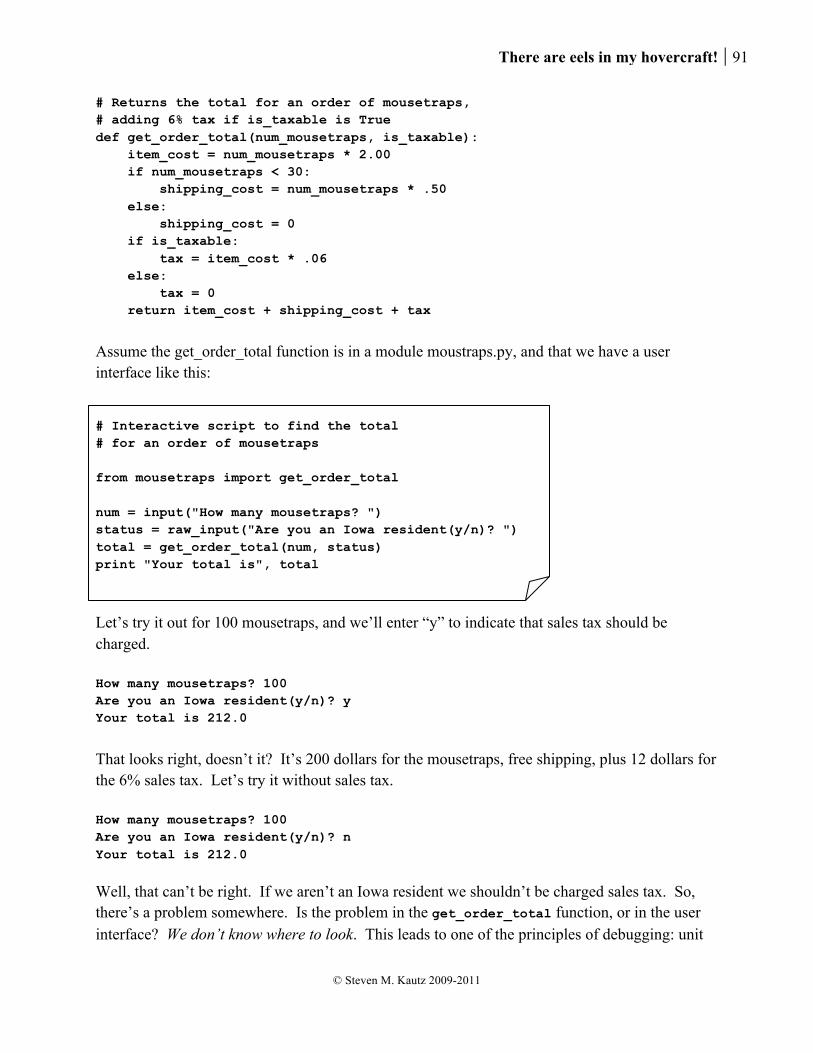
There are eels in my hovercraft! 91
© Steven M. Kautz 2009-2011
# Returns the total for an order of mousetraps, # adding 6% tax if is_taxable is True def get_order_total(num_mousetraps, is_taxable): item_cost = num_mousetraps * 2.00 if num_mousetraps < 30: shipping_cost = num_mousetraps * .50 else: shipping_cost = 0 if is_taxable: tax = item_cost * .06 else: tax = 0 return item_cost + shipping_cost + tax
Assume the get_order_total function is in a module moustraps.py, and that we have a user interface like this: # Interactive script to find the total # for an order of mousetraps from mousetraps import get_order_total num = input("How many mousetraps? ") status = raw_input("Are you an Iowa resident(y/n)? ") total = get_order_total(num, status) print "Your total is", total
Let’s try it out for 100 mousetraps, and we’ll enter “y” to indicate that sales tax should be charged. How many mousetraps? 100 Are you an Iowa resident(y/n)? y Your total is 212.0
That looks right, doesn’t it? It’s 200 dollars for the mousetraps, free shipping, plus 12 dollars for the 6% sales tax. Let’s try it without sales tax. How many mousetraps? 100 Are you an Iowa resident(y/n)? n Your total is 212.0
Well, that can’t be right. If we aren’t an Iowa resident we shouldn’t be charged sales tax. So, there’s a problem somewhere. Is the problem in the get_order_total function, or in the user interface? We don’t know where to look. This leads to one of the principles of debugging: unit

92 Bugs!
© Steven M. Kautz 2009-2011
test the components before you test the whole system. Why? If we first unit test the get_order_total function and we are confident that it has no errors, then that reduces the number of places we have to look for the cause of the error in the user interface. It is not hard to come up with a quick test for get_order_total: # Unit test for get_order_total from mousetraps import get_order_total print "10 with no tax, expected 25.00, actual", get_order_total(10, False) print "100 with no tax, expected 200.00, actual", get_order_total(100, False) print "10 with tax, expected 26.20, actual", get_order_total(10, True) print "100 with tax, expected 212.00, actual", get_order_total(100, True)
This gives us some confidence not only that the get_order_total function is correct, but also that we know how to call it correctly. Now, if we are sure the function works correctly, why do we get the wrong answers from the user interface? It looks like tax is being added even when we enter “n”. One thing we can do to help track down what’s happening is to put a couple of temporary print statements in the get_order_total function where it computes the tax: if is_taxable: print "adding tax" tax = item_cost * .06 else: print "setting tax to zero" tax = 0
We can run the user interface and try answering “n” again. How many mousetraps? 100 Are you an Iowa resident(y/n)? n adding tax Your total is 212.0
And it’s clear that the “if” block is being executed and is adding tax. Hmm. Let’s add another print statement and see what the value of is_taxable is when we check it: print "is_taxable has value", is_taxable if is_taxable: print "adding tax"

There are eels in my hovercraft! 93
© Steven M. Kautz 2009-2011
tax = item_cost * .06 else: print "setting tax to zero" tax = 0
We try the user interface again to see what’s going on: How many mousetraps? 100 Are you an Iowa resident(y/n)? n is_taxable has value n adding tax Your total is 212.0
Aha! We’re expecting the variable is_taxable to have a True/False value, but it is the letter “n”. We can fix that in the user interface. We have to check the value entered by the user and call the get_order_total function using an argument of either True or False, just as we did in the unit test. # Interactive script to find the total # for an order of mousetraps from mousetraps import get_order_total num = input("How many mousetraps? ") status = raw_input("Are you an Iowa resident(y/n)? ") if status == "y": total = get_order_total(num, True) else: total = get_order_total(num, False) print "Your total is", total
Don’t forget to take the extra print statements out of the get_order_total function. You might wonder, why did the interpreter execute the “if” block when is_taxable had the value “n”? That is a strange feature of Python. Logically the condition for an if-statement should be an expression that’s True or False. But Python will actually allow any expression to be used. For strings, an empty string is treated as False, and any nonempty string is treated as True. For numbers, a value of zero is treated as False, and nonzero values act like True. In general, to avoid confusion, we should always make sure to use boolean expressions in conditional statements.

94 Binary numbers and data encoding
© Steven M. Kautz 2009-2011
12. Binary numbers and data encoding Part of what we want to accomplish in this course is to develop some background on how a computer works. We have mentioned before that everything your computer does is represented by millions of tiny little electrical switches. We can think of a switch that is “off” as the value zero, and a switch that is “on” as the value 1. Ok, so we have a whole bunch of ones and zeros. Big deal. So how does a machine do things like perform arithmetic, edit words, process images, or generate music? The real information – numbers, text, images, sounds – has to be encoded somehow into zeros and ones.
12.1. Binary numbers
The first step is to see how we can represent whole numbers and do arithmetic using zeros and ones. The way we usually write numbers is called the “decimal” or “base 10” system. We have 10 symbols, the digits 0 through 9. If you write “4”, by itself, it means four, but if you write “425”, the digit “4” actually means “four times a hundred”. The value of a given digit depends on the place value for its position in a number. 100’s place, 10’s place, 1’s place 425 4 times 100 plus 2 times 10 plus 5 The place values are always powers of 10, which is why this system is called “base 10”. In the “binary” or “base 2” system, the idea is the same, but the place values are different. They are powers of 2 instead of powers of 10. For example, suppose we have a binary number 101101. What value is that? Just write the powers of 2 underneath it, and add up the place values where you see a “1” 1 0 1 1 0 1 32 16 8 4 2 1
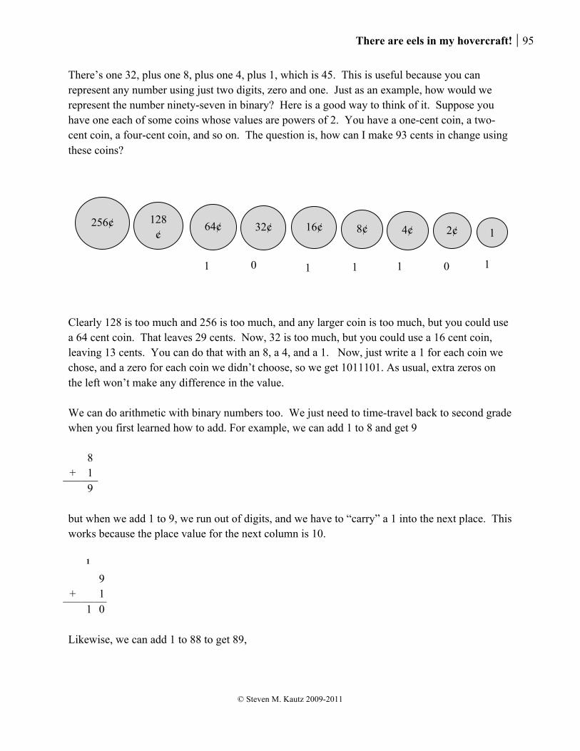
There are eels in my hovercraft! 95
© Steven M. Kautz 2009-2011
There’s one 32, plus one 8, plus one 4, plus 1, which is 45. This is useful because you can represent any number using just two digits, zero and one. Just as an example, how would we represent the number ninety-seven in binary? Here is a good way to think of it. Suppose you have one each of some coins whose values are powers of 2. You have a one-cent coin, a two-cent coin, a four-cent coin, and so on. The question is, how can I make 93 cents in change using these coins?
Clearly 128 is too much and 256 is too much, and any larger coin is too much, but you could use a 64 cent coin. That leaves 29 cents. Now, 32 is too much, but you could use a 16 cent coin, leaving 13 cents. You can do that with an 8, a 4, and a 1. Now, just write a 1 for each coin we chose, and a zero for each coin we didn’t choose, so we get 1011101. As usual, extra zeros on the left won’t make any difference in the value. We can do arithmetic with binary numbers too. We just need to time-travel back to second grade when you first learned how to add. For example, we can add 1 to 8 and get 9
8 + 1
9 but when we add 1 to 9, we run out of digits, and we have to “carry” a 1 into the next place. This works because the place value for the next column is 10.
1 9
+ 1 1 0
Likewise, we can add 1 to 88 to get 89,
256¢ 128¢
64¢ 32¢ 16¢ 8¢ 4¢ 2¢ 1¢
1 1 1 1 1 0 0

96 Binary numbers and data encoding
© Steven M. Kautz 2009-2011
8 8 + 1
8 9 But when we add 1 to 89, we run out of digits and have to carry a 1 into the next place.
1 8 9
+ 1 9 0
If we continue this process up to 99, then what happens? We carry a 1 into the next place and try to add it to 9, and we have to carry again:
1 1 9 9
+ 1 1 0 0
So let’s imagine how it works when you want to do everything with two digits, zero and one. We can start at zero and add 1, to get 1:
0 + 1
1 then when we add 1, we run out of digits, and carry a “1” into the next place. For this to be right, the value of “one zero” must be 2 – which it is, since the next column has place value 2.
1 1
+ 1 1 0
Let’s keep going. “one zero” plus one would be “one one”, which must have value 3.
1 0
+ 1
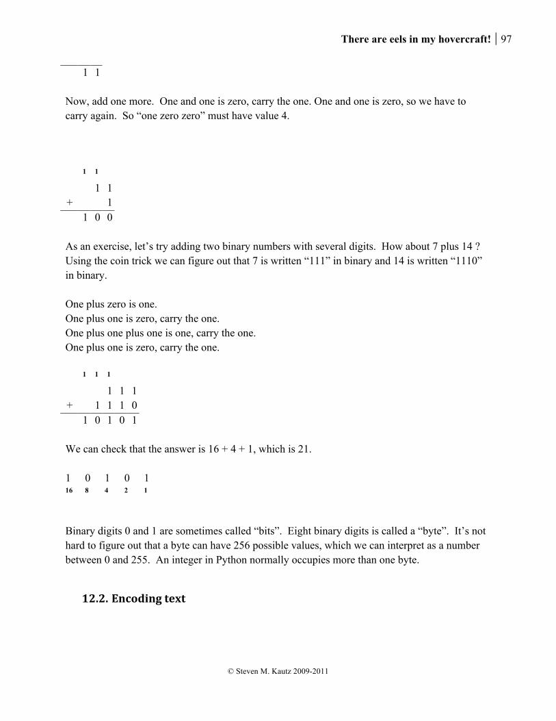
There are eels in my hovercraft! 97
© Steven M. Kautz 2009-2011
1 1 Now, add one more. One and one is zero, carry the one. One and one is zero, so we have to carry again. So “one zero zero” must have value 4.
1 1 1 1
+ 1 1 0 0
As an exercise, let’s try adding two binary numbers with several digits. How about 7 plus 14 ? Using the coin trick we can figure out that 7 is written “111” in binary and 14 is written “1110” in binary. One plus zero is one. One plus one is zero, carry the one. One plus one plus one is one, carry the one. One plus one is zero, carry the one.
1 1 1 1 1 1
+ 1 1 1 0 1 0 1 0 1
We can check that the answer is 16 + 4 + 1, which is 21. 1 0 1 0 1 16 8 4 2 1
Binary digits 0 and 1 are sometimes called “bits”. Eight binary digits is called a “byte”. It’s not hard to figure out that a byte can have 256 possible values, which we can interpret as a number between 0 and 255. An integer in Python normally occupies more than one byte.
12.2. Encoding text

98 Binary numbers and data encoding
© Steven M. Kautz 2009-2011
Binary notation works well for whole numbers. But what about text? The idea is to decide on some way to associate each character with a number or “code”. A list of characters and the associated numbers is called a character set. There are many character sets, because each written language has its own symbols. Historically one of the “original” character sets is called ASCII (pronounced “ASK-ee”). It originated in the United States and therefore it has only the symbols for the letters and punctuation of the English language. There are 127 values in ASCII, so each character can be encoded with one byte. Here is a summary of the ASCII codes. Numbers 0 through 31 are the so-called “control” characters. They aren’t printable, but they do things like mark the end of a line. We’ll encounter a few of them later. Number 32 is the space character, and then the next fifteen are for various symbols and punctuation marks. Then numbers 48 through 57 are the digits zero through nine, followed by some more punctuation. 65 through 90 are the uppercase letters, followed by still more punctuation, and then codes 97 through 122 are the lowercase letters. ASCII codes Description Characters 0-31 Control characters 32 Space character 33-47 Symbols and punctuation ! " # $ % & ’ ( ) * + , - . / 48-57 Digits 0 - 9 0123456789 58-64 Symbols and punctuation : ; < = > ? @ 65-90 Uppercase letters ABCDEFGHIJKLMNOPQRSTUVWXYZ 91-96 Symbols and punctuation [ \ ] ^ _ ` 97-122 Lowercase letters abcdefghijklmnopqrstuvwxyz 123 - 126 Punctuation { | } ~ 127 Control character You might notice that there seems to be no rhyme or reason to any of this, and you are mostly right. The encoding is based on choices that might have made sense back in the 1960s, but make no difference now. ASCII is still important because almost every character set in use nowadays are an extension of ASCII. For example, the Latin-1 character set used in European countries has 256 values. The first 127 are the same as ASCII, and the rest of the values define encodings for the special characters used in European languages. Since there are only 256 possible values, a character can be represented as one byte. More complex character sets for non-European languages may require more than one byte per character. Another good question is: why do we care about any of this? In general, we don’t ever need to know the actual ASCII code for a character. But it is important to know something about their ordering. The main thing we have to understand is what’s going on when we compare strings.
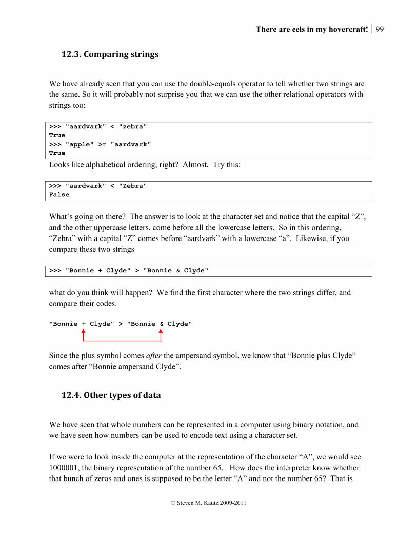
There are eels in my hovercraft! 99
© Steven M. Kautz 2009-2011
12.3. Comparing strings
We have already seen that you can use the double-equals operator to tell whether two strings are the same. So it will probably not surprise you that we can use the other relational operators with strings too: >>> "aardvark" < "zebra" True >>> "apple" >= "aardvark" True
Looks like alphabetical ordering, right? Almost. Try this: >>> "aardvark" < "Zebra" False
What’s going on there? The answer is to look at the character set and notice that the capital “Z”, and the other uppercase letters, come before all the lowercase letters. So in this ordering, “Zebra” with a capital “Z” comes before “aardvark” with a lowercase “a”. Likewise, if you compare these two strings >>> "Bonnie + Clyde" > "Bonnie & Clyde"
what do you think will happen? We find the first character where the two strings differ, and compare their codes. "Bonnie + Clyde" > "Bonnie & Clyde"
Since the plus symbol comes after the ampersand symbol, we know that “Bonnie plus Clyde” comes after “Bonnie ampersand Clyde”.
12.4. Other types of data
We have seen that whole numbers can be represented in a computer using binary notation, and we have seen how numbers can be used to encode text using a character set. If we were to look inside the computer at the representation of the character “A”, we would see 1000001, the binary representation of the number 65. How does the interpreter know whether that bunch of zeros and ones is supposed to be the letter “A” and not the number 65? That is
100 Binary numbers and data encoding
© Steven M. Kautz 2009-2011
why every value has to have a type. If the bits 1000001 are associated with type int, then it’s the number 65. If the same bits are associated with the type string, then it’s the character “A”. Floating-point numbers have their own encoding into zeros and ones that is very different from the encoding for integers. If the same bits are associated with the type “float”, then the value, believe it or not, is 9.1 times 10 to the minus 44th power. . Likewise every other kind of data has to have some kind of encoding. For example, an image that you see on your screen is really a rectangular grid of “dots”, called pixels. The appearance of each pixel is typically encoded as three bytes representing the intensity of red, green, and blue at that location in the image. (Sometimes there is a fourth byte for transparency.)
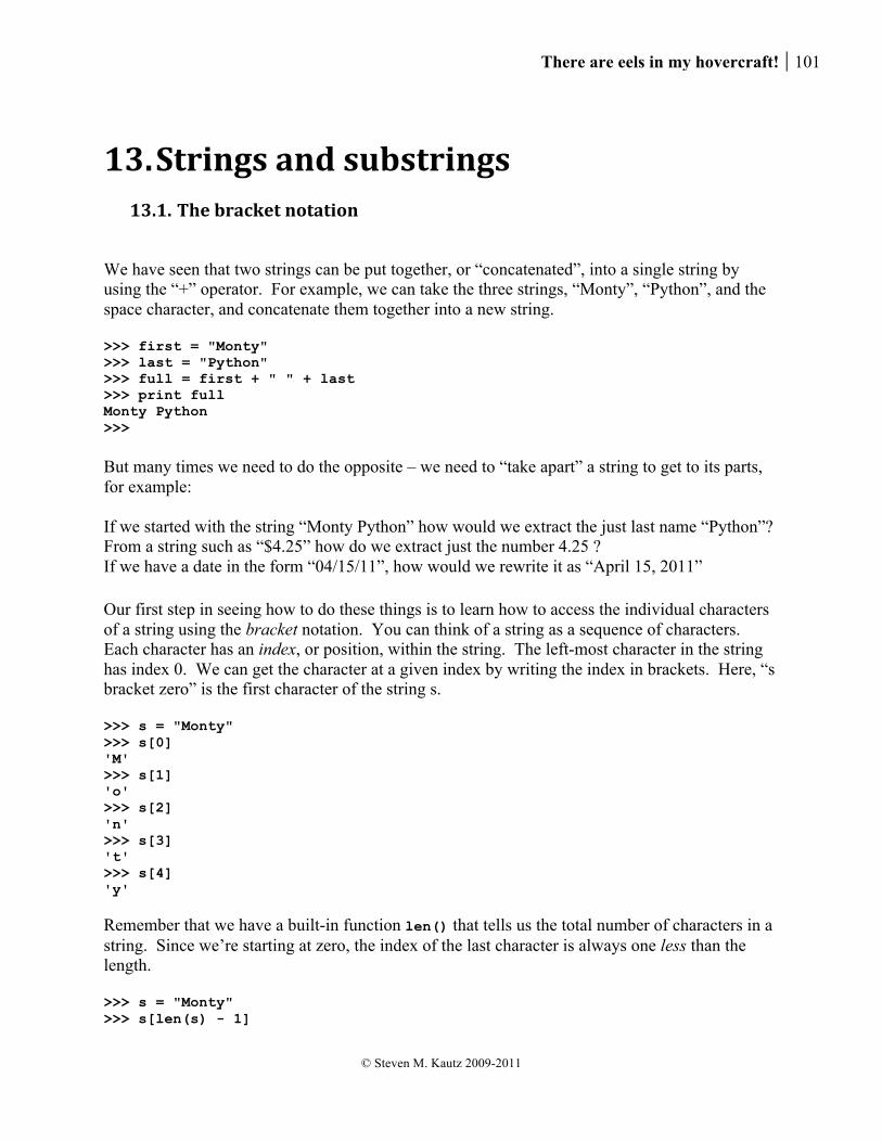
There are eels in my hovercraft! 101
© Steven M. Kautz 2009-2011
13. Strings and substrings 13.1. The bracket notation
We have seen that two strings can be put together, or “concatenated”, into a single string by using the “+” operator. For example, we can take the three strings, “Monty”, “Python”, and the space character, and concatenate them together into a new string. >>> first = "Monty" >>> last = "Python" >>> full = first + " " + last >>> print full Monty Python >>> But many times we need to do the opposite – we need to “take apart” a string to get to its parts, for example: If we started with the string “Monty Python” how would we extract the just last name “Python”? From a string such as “$4.25” how do we extract just the number 4.25 ? If we have a date in the form “04/15/11”, how would we rewrite it as “April 15, 2011” Our first step in seeing how to do these things is to learn how to access the individual characters of a string using the bracket notation. You can think of a string as a sequence of characters. Each character has an index, or position, within the string. The left-most character in the string has index 0. We can get the character at a given index by writing the index in brackets. Here, “s bracket zero” is the first character of the string s. >>> s = "Monty" >>> s[0] 'M' >>> s[1] 'o' >>> s[2] 'n' >>> s[3] 't' >>> s[4] 'y' Remember that we have a built-in function len() that tells us the total number of characters in a string. Since we’re starting at zero, the index of the last character is always one less than the length. >>> s = "Monty" >>> s[len(s) - 1]
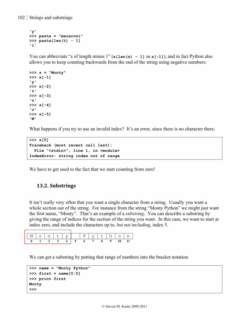
102 Strings and substrings
© Steven M. Kautz 2009-2011
'y' >>> pasta = "macaroni" >>> pasta[len(t) - 1] 'i' You can abbreviate “s of length minus 1” (s[len(s) – 1] as s[-1]), and in fact Python also allows you to keep counting backwards from the end of the string using negative numbers: >>> s = "Monty" >>> s[-1] 'y' >>> s[-2] 't' >>> s[-3] 'n' >>> s[-4] 'o' >>> s[-5] 'M' What happens if you try to use an invalid index? It’s an error, since there is no character there. >>> s[5] Traceback (most recent call last): File "<stdin>", line 1, in <module> IndexError: string index out of range
We have to get used to the fact that we start counting from zero!
13.2. Substrings
It isn’t really very often that you want a single character from a string. Usually you want a whole section out of the string. For instance from the string “Monty Python” we might just want the first name, “Monty”. That’s an example of a substring. You can describe a substring by giving the range of indices for the section of the string you want. In this case, we want to start at index zero, and include the characters up to, but not including, index 5. M o n t y P y t h o n 0 1 2 3 4 5 6 7 8 9 10 11
We can get a substring by putting that range of numbers into the bracket notation. >>> name = "Monty Python" >>> first = name[0:5] >>> print first Monty >>>
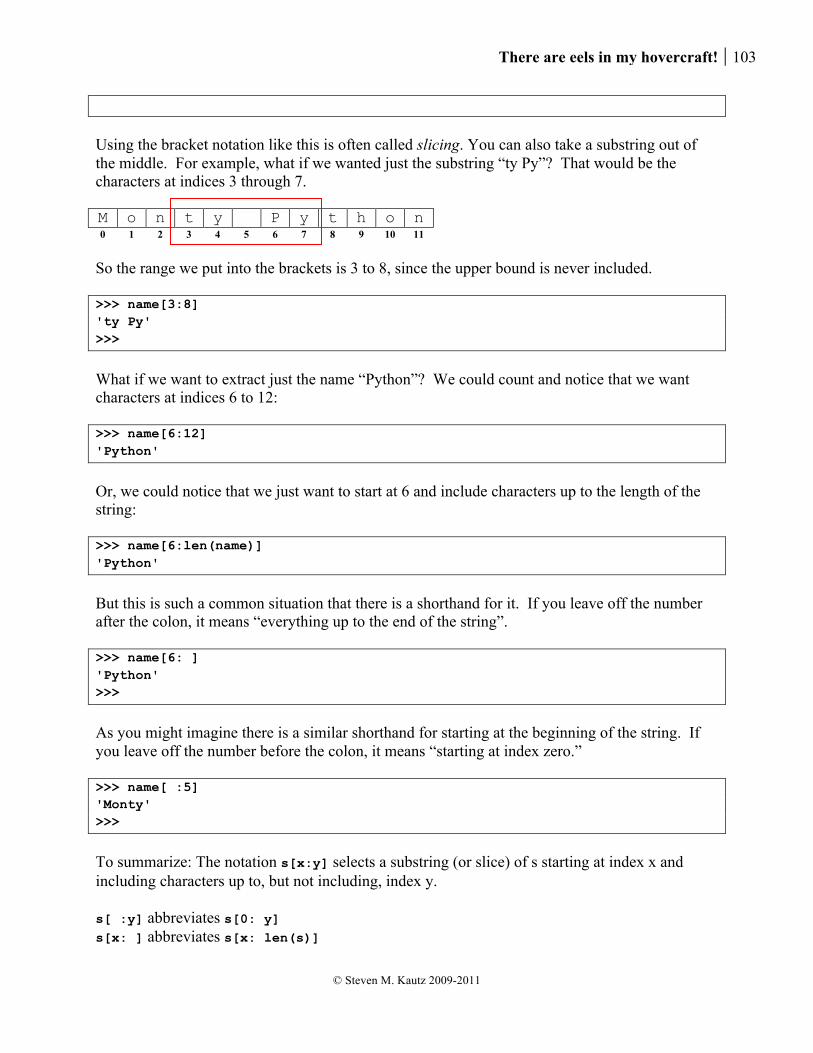
There are eels in my hovercraft! 103
© Steven M. Kautz 2009-2011
Using the bracket notation like this is often called slicing. You can also take a substring out of the middle. For example, what if we wanted just the substring “ty Py”? That would be the characters at indices 3 through 7. M o n t y P y t h o n 0 1 2 3 4 5 6 7 8 9 10 11
So the range we put into the brackets is 3 to 8, since the upper bound is never included. >>> name[3:8] 'ty Py' >>>
What if we want to extract just the name “Python”? We could count and notice that we want characters at indices 6 to 12: >>> name[6:12] 'Python'
Or, we could notice that we just want to start at 6 and include characters up to the length of the string: >>> name[6:len(name)] 'Python'
But this is such a common situation that there is a shorthand for it. If you leave off the number after the colon, it means “everything up to the end of the string”. >>> name[6: ] 'Python' >>>
As you might imagine there is a similar shorthand for starting at the beginning of the string. If you leave off the number before the colon, it means “starting at index zero.” >>> name[ :5] 'Monty' >>>
To summarize: The notation s[x:y] selects a substring (or slice) of s starting at index x and including characters up to, but not including, index y. s[ :y] abbreviates s[0: y] s[x: ] abbreviates s[x: len(s)]
104 Strings and substrings
© Steven M. Kautz 2009-2011
It is worth noticing that if the range doesn’t really describe part of the string, it isn’t an error – you just get an empty string as the result. >>> name[42:137] ''
Here’s another observation: suppose s is any string and i is any number. What is s[ :i] + s[i: ]? It’s always the same as the original string s. (picture?) As an example, let’s write a function that takes any string and replaces its first letter with the letter “b”. For instance, “see” would become “bee”. It is tempting to try it like this, where we just assign a new value to the first character. def replace_b(word): word[0] = "b"
But when we try to use it, we get an error! word[0] = "b" TypeError: 'str' object does not support item assignment
It turns out that once a string is created, it can’t be modified. We say that strings are immutable. What we have to do is just create the result we want as a brand new string. We take a substring of the given word that doesn’t include the first letter, and then concatenate a “b” at the beginning: def replace_b(word): return "b" + word[1: ]
13.3. Other kinds of sequences
A string is a kind of a sequence. The individual elements of the sequence are characters. Think about some of the properties of a string we have just been using:
1. It has a length, which we can determine with the len() function 2. Each element has a position or index in the sequence, 0 through the length – 1. 3. We can use the bracket notation to access an individual element according to its index, or
to take a “slice” using a range of indices
There are eels in my hovercraft! 105
© Steven M. Kautz 2009-2011
There are sequences of other types too, that also have those same three properties. In Python, a list is a sequence of values of any type. You can create a list just by writing the values, separated by commas, and enclosed in square brackets. For example, here is a simple list of five numbers: >>> my_list = [17, 42, 137, 19, 21] >>> print my_list [17, 42, 137, 19, 21]
If you examine a list in the shell or using a print statement, it is displayed in the same way; the values are separated by commas and the whole thing is within square brackets. We can use the len function to determine its length, and the bracket notation to examine its elements: >>> len(my_list) 5 >>> my_list[0] 17 >>> my_list[2] 137
We can also take a “slice”: >>> my_list[:3] [17, 42, 137] >>>
You can also create lists of other types. Here is an example of a list of strings. >>> ducks = ["Huey", "Louie", "Dewey"]
Now, let’s put together what we’ve seen so far to do something new. We’ll write a function that converts a date such as “04/15/11” into the form “April 15, 2011”. We’re assuming here that the month, day, and year are always exactly two digits. We can use slicing to get the two digits corresponding to the day, which occupy indices 3 and 4. day = date[3:5]
And we can do the same thing with the year, which is the last two digits, using a negative index of -2 to indicate “the second to last character”. year = date[-2:]

106 Strings and substrings
© Steven M. Kautz 2009-2011
And we can get the month number the same way. But how do we convert it to the name of the month? Well, we could use an “if” statement with a lot of “elifs”. But here is another idea. Let’s create a sequence of strings that has the month names in order: names = ["January", "February", "March", "April", \ "May", "June", "July", "August", \ "September", "October", "November", "December"] Now we know that names[0] is January, names[1] is February, and so on. So we just have to convert the month number into an index we can use in this list. When we write dates, we use numbers 1 through 12, so we’ll need to subtract 1 because the list indices go from 0 through 11. Remember to convert from string to int first. month = date[0:2] index = int(month) - 1 month_name = names[index] Finally we have to put the month name, the day, and the year together into a new string result = month_name + " " + day + ", " + "20" + year The completed function looks like this: # Converts a date string of the form "04/15/2011" into one # of the form "April 15, 2011" def convert_date(date): day = date[3:5] year = "20" + date[-2:] names = ["January", "February", "March", "April", \ "May", "June", "July", "August", \ "September", "October", "November", "December"] month = date[0:2] index = int(month) - 1 month_name = names[index] result = month_name + " " + day + ", " + year return result
There are eels in my hovercraft! 107
© Steven M. Kautz 2009-2011
14. String operations 14.1. String methods
In the last chapter we learned how to use the bracket notation to access the individual characters of a string and to get a substring, or “slice”, from a string. In this chapter we want to begin exploring some of the other operations on strings that are available in the Python libraries. Let’s start with an example. There is an operation called “upper” that takes a string and gives you a new string that is the same as the first one, but with all the lower-case characters converted to upper-case. Suppose we have the string “Steve” stored in a variable s. >>> s = "Steve" Then we execute the statement “t gets s dot upper”, >>> t = s.upper() The variable “t” now contains the value “STEVE” in capital letters. >>> print t STEVE >>> print s Steve Notice that the string s is not changed. Look at the peculiar notation, “s dot upper”: s.upper() A function used this way is called a method. The string you want the function to operate on is given first, followed by a dot, and then the function name. In contrast, when we call a built-in function like len, we have to provide the string as an argument: >>> len(s) 5
Most of the operations you can perform on strings are implemented as methods and are invoked using this “dot” notation. We sometimes call the string before the dot the “target” of the method, because that’s the string the method is going to act upon. The other thing to notice about this example is that the original string “s” is not modified. In fact, none of the string operations actually modify the target string - strings are immutable, remember?
108 String operations
© Steven M. Kautz 2009-2011
Here is an overview of the most useful methods on strings. We have just seen the method upper(). There is also a method lower() that returns the target string with any upper-case letters converted to lower-case. >>> s = "Steve" >>> t = s.lower() >>> t 'steve' The method capitalize() returns a string with just the first letter converted to uppercase and the rest in lowercase: >>> s = "STEVE" >>> t = s.capitalize() >>> t 'Steve'
The method strip() returns a new string with all “whitespace” trimmed from the beginning and end of your target string. Remember that “whitespace” includes space characters, tab characters, and newline characters. >>> x = " Hello, world " >>> y = x.strip() >>> y 'Hello, world'
These four methods, upper(), lower(), capitalize(), and strip(), all return a new string. The next example is a method that returns an integer. The find() method has one argument, which is a character or string, say “t”. If “t” is a substring of your target string, then the find() method returns the first index at which “t” occurs. If t doesn’t occur at all, then find() returns -1. >>> s = "Mississippi" >>> s.find("ss") 2 >>> s.find("w") -1 The startswith() method is also related to substrings. Like find(), it has one string argument “t”, but it returns a boolean value. It returns True if the very beginning of your target string exactly matches “t”. >>> answer = "yes" >>> answer.startswith("y") True
Logically, you could say that

There are eels in my hovercraft! 109
© Steven M. Kautz 2009-2011
s.startswith(t)
is true if and only if s.find(t) == 0
It will probably not surprise you to learn that there is a similar function endswith() that returns True if the end of the target exactly matches the argument string. >>> s = "Mississippi" >>> s.endswith("ippi") True
We’ll conclude this summary with one more method, called split(), that is very useful for processing text. The return value of split() is not a single value, but is a list of strings. The idea is that you take a string containing multiple items having one or more spaces between them, like words in a sentence: >>> s = "There are eels in my hovercraft!"
Then the result of invoking split() is a list of the individual words: >>> words = s.split() >>> words ['There', 'are', 'eels', 'in', 'my', 'hovercraft!']
As we saw in the last chapter, you can use the bracket notation to get the individual elements of the sequence. >>> first_word = words[0] >>> first_word 'There'
14.2. Summary of string methods
The box below contains a summary of the methods we have discussed. Note that there are many more which we have not discussed. You can see them all in section 5.6.1 of the Python Library Reference, available at http://docs.python.org/library/stdtypes.html#string-methods s.upper() returns a string created from s by converting characters to uppercase s.lower() returns a string created from s by converting characters to lowercase s.capitalize() returns a string created from s by capitalizing just the first letter
110 String operations
© Steven M. Kautz 2009-2011
s.strip() returns a string created from s by removing any white space at the beginning or end s.find(t) returns the first index of substring t in string s (-1 if it doesn’t occur) s.startswith(t) returns True if string s starts with string t s.endswith(t) returns True if string s ends with string t s.split() returns a sequence of strings obtained from substrings of s that are separated by whitespace In addition to the methods above, remember there are three built-in functions that are important for working with strings str(x) returns a string representing the number or object x int(s) returns the int value represented by string s float(s) returns the floating-point value represented by string s Note that the last two can generate errors: int(“42”) is the value 42, but int(“42x”) is an error.
14.3. Chaining methods
Here is an example. In some of our interactive scripts we ask a user to enter “y” for yes and “n” for no, and then check whether the response is equal to “y”. status = raw_input("Are you an Iowa resident(y/n)? ") if status == "y": # etc
This works fine if the user is careful to enter exactly the single character, lower-case “y”. But what if they enter an upper-case “Y”, or if they type “yes” or “Yes”, or accidentally add an extra space before or after the response. We’d probably want to count all those responses as a “yes” answer too. So we can make our code more robust by stripping off the whitespace from the response, using the strip() method. status = raw_input("Are you an Iowa resident(y/n)? ") status2 = status.strip()
Then, we can convert to lowercase: status3 = status2.lower() Finally, we check whether the response starts with “y”: if status3.startswith("y"): # etc
The thing to notice is that since the value of status.strip() is just a string, we can invoke the lower() method on it directly, without the need for the variable status2.
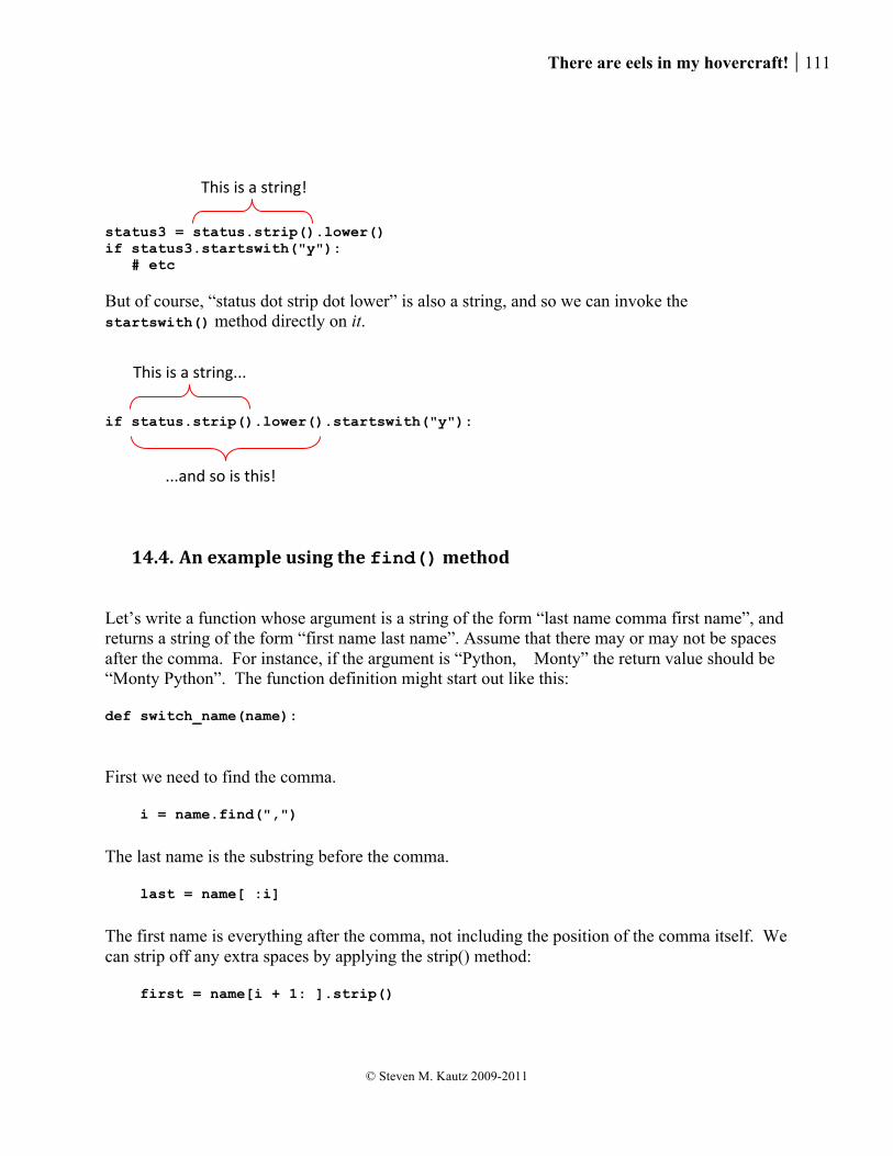
There are eels in my hovercraft! 111
© Steven M. Kautz 2009-2011
status3 = status.strip().lower() if status3.startswith("y"): # etc But of course, “status dot strip dot lower” is also a string, and so we can invoke the startswith() method directly on it. if status.strip().lower().startswith("y"):
14.4. An example using the find() method
Let’s write a function whose argument is a string of the form “last name comma first name”, and returns a string of the form “first name last name”. Assume that there may or may not be spaces after the comma. For instance, if the argument is “Python, Monty” the return value should be “Monty Python”. The function definition might start out like this: def switch_name(name):
First we need to find the comma. i = name.find(",")
The last name is the substring before the comma. last = name[ :i]
The first name is everything after the comma, not including the position of the comma itself. We can strip off any extra spaces by applying the strip() method: first = name[i + 1: ].strip()
This is a string!
This is a string...
...and so is this!

112 String operations
© Steven M. Kautz 2009-2011
Finally, we put the first and last names together with a space in between. return first + " " + last
14.5. Format strings
In our examples so far we have ignored the issue of how to format a number so it prints with exactly two decimal places, or how to line things up in columns. For these and related problems we need format strings. The idea is just to create a string containing “placeholders”, and then supply the values to fill in. The placeholders can be used to help format the output the way you want it. The placeholders are called format specifiers and always start with the “%” symbol. These are the most common forms: %s placeholder for a string %d placeholder for an int %f placeholder for a float Try this in the interpreter. >>> fmt = "My name is %s and I ate %d pies" >>> print fmt My name is %s and I ate %d pies As you can see, fmt is just a string. In order to replace the “percent sign” specifiers with something meaningful, you follow the format string with another “%” symbol and then a list of values in parentheses. The value of the resulting expression is a string that you can print or assign to a variable: >>> s = fmt % ("Steve", 42) >>> print s My name is Steve and I ate 42 pies The values in parentheses are substituted for the placeholders. "My name is %s and I ate %d pies" % ("Steve", 42) So as you might imagine the number of values you supply in the parentheses has to match the number of placeholders, and the values have to be the right type. If there is only one value, the parentheses are optional. The amount of space taken up by a value is called the field width. You can specify the field width by putting a number after the “%”. The field automatically expands to fit the value you supply, so a field width of 1 just means “take up the minimum amount of space”, which is the default. For example, here we are allocating 10 spaces for the number 42.

There are eels in my hovercraft! 113
© Steven M. Kautz 2009-2011
>>> print "I ate %10d pies" % 42 I ate 42 pies For floats you can also specify the number of decimal places; for example %6.2f means “allow a total of 6 spaces and display 2 decimal places.” This will round the number to two decimal places and print it with the minimum amount of space: >>> print "The price of a %s is $%1.2f" % ("pie", 3.14159) The price of a pie is $3.14 This will allocate 6 spaces for the number: >>> print "The price of a %s is $%6.2f" % ("pie", 3.14159) The price of a pie is $ 3.14 By repeating specifiers you can get things lined up in columns. Here we are printing everything in columns 12 characters wide. >>> print "%12d%12d%12d%12d" % (2, 4, 6, 8) 2 4 6 8 >>> print "%12s%12s%12s%12s" % ("Who", "do", "we", "appreciate") Who do we appreciate Notice that the default is to print the value “right-justified” – that is, at the right side of its column. You can force the value to be “left-justified” by putting a minus sign in front of the field width: >>> print "%-12d%-12d%-12d%-12d" % (2, 4, 6, 8) 2 4 6 8
One more useful trick: When you put the field width in a format specifier, you can put a zero first. This means that any extra spaces in the field will be filled with zeros: >>> print "I ate %5d pies" % 42 I ate 42 pies >>> print "I ate %05d pies" % 42 I ate 00042 pies

114 For-loops
© Steven M. Kautz 2009-2011
15. For-‐loops 15.1. Water the plants
In this chapter we are going to start writing loops – statements that cause an action to be repeated. The simplest kind of repeated action comes up when you start with a known set or sequence of things, and you have to perform some action once for each thing. This happens all the time in life, for example:
Put frosting and sprinkles on each cupcake. Deliver a newspaper to each house on the block. Call each person on the list and invite them to the party. Water the houseplants.
We could make the language more uniform and precise by starting each sentence with the word “for:” and referring to each item using a variable:
For each cupcake c on the plate, put frosting and sprinkles on c. For each house h on the block, deliver a newspaper to h. For each person p on the list, invite p to the party. For each plant x in the house, water x.
Suppose you’ve made a dozen cupcakes and you carry out the instructions:
For each cupcake c, put frosting and sprinkles on c.
You’ll perform the action in the second line12 times, and each time you do it, you do it for a different cupcake “c”. That is exactly how a for-loop works in Python. You have a sequence of values, and you want to execute some statements once for each value. For our first example, assume we have a sequence of some integers. values = [2, 4, 6, 8, 10]
We can write a for-loop that just prints each value by itself:
There are eels in my hovercraft! 115
© Steven M. Kautz 2009-2011
for v in values: print v
The output from running this as a script would be: 2 4 6 8 10
You can see that the line print v
actually executes 5 times, and each time it executes, the variable “v” holds the next value in the sequence. Maybe instead of printing each value in the sequence, we want to add them up. Logically we want to say for each value v in the sequence add v to the total where the total starts out at zero. values = [2, 4, 6, 8, 10] total = 0 for val in values: total = total + val print total
Notice that as usual, indentation is used to show which statements are part of the loop body, and which are after. In this case the last line, “print total”, is not part of the loop body, so it only executes when the loop is finished. If we run this as a script, the output is 30.
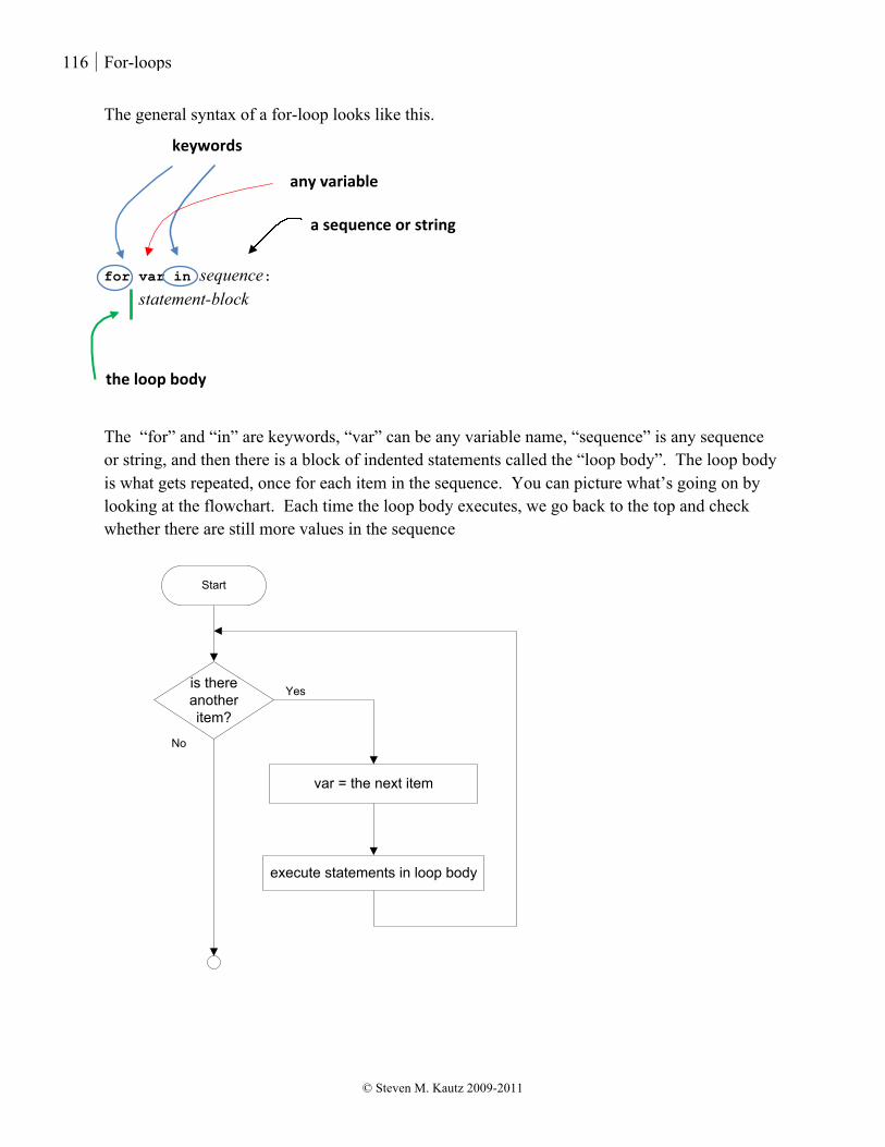
116 For-loops
© Steven M. Kautz 2009-2011
The general syntax of a for-loop looks like this. for var in sequence: statement-block The “for” and “in” are keywords, “var” can be any variable name, “sequence” is any sequence or string, and then there is a block of indented statements called the “loop body”. The loop body is what gets repeated, once for each item in the sequence. You can picture what’s going on by looking at the flowchart. Each time the loop body executes, we go back to the top and check whether there are still more values in the sequence
is there another item?
No
Yes
var = the next item
execute statements in loop body
Start
keywords
any variable
a sequence or string
the loop body
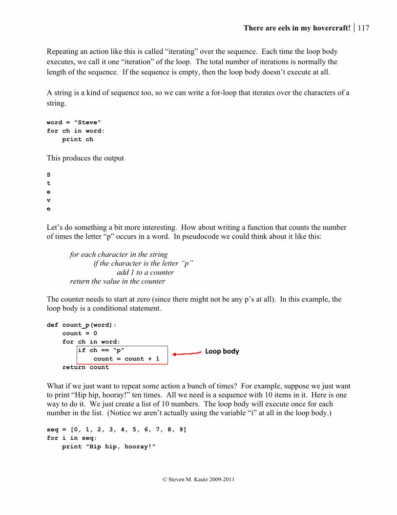
There are eels in my hovercraft! 117
© Steven M. Kautz 2009-2011
Repeating an action like this is called “iterating” over the sequence. Each time the loop body executes, we call it one “iteration” of the loop. The total number of iterations is normally the length of the sequence. If the sequence is empty, then the loop body doesn’t execute at all. A string is a kind of sequence too, so we can write a for-loop that iterates over the characters of a string. word = "Steve" for ch in word: print ch
This produces the output S t e v e
Let’s do something a bit more interesting. How about writing a function that counts the number of times the letter “p” occurs in a word. In pseudocode we could think about it like this:
for each character in the string if the character is the letter “p” add 1 to a counter return the value in the counter
The counter needs to start at zero (since there might not be any p’s at all). In this example, the loop body is a conditional statement. def count_p(word): count = 0 for ch in word: if ch == "p" count = count + 1 return count
What if we just want to repeat some action a bunch of times? For example, suppose we just want to print “Hip hip, hooray!” ten times. All we need is a sequence with 10 items in it. Here is one way to do it. We just create a list of 10 numbers. The loop body will execute once for each number in the list. (Notice we aren’t actually using the variable “i” at all in the loop body.) seq = [0, 1, 2, 3, 4, 5, 6, 7, 8, 9] for i in seq: print "Hip hip, hooray!"
Loop body
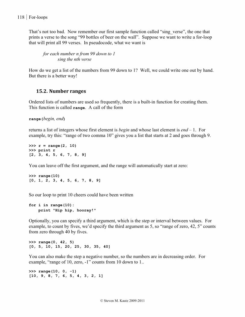
118 For-loops
© Steven M. Kautz 2009-2011
That’s not too bad. Now remember our first sample function called “sing_verse”, the one that prints a verse to the song “99 bottles of beer on the wall”. Suppose we want to write a for-loop that will print all 99 verses. In pseudocode, what we want is
for each number n from 99 down to 1 sing the nth verse
How do we get a list of the numbers from 99 down to 1? Well, we could write one out by hand. But there is a better way!
15.2. Number ranges
Ordered lists of numbers are used so frequently, there is a built-in function for creating them. This function is called range. A call of the form range(begin, end) returns a list of integers whose first element is begin and whose last element is end – 1. For example, try this: “range of two comma 10” gives you a list that starts at 2 and goes through 9. >>> r = range(2, 10) >>> print r [2, 3, 4, 5, 6, 7, 8, 9] You can leave off the first argument, and the range will automatically start at zero: >>> range(10) [0, 1, 2, 3, 4, 5, 6, 7, 8, 9] So our loop to print 10 cheers could have been written for i in range(10): print "Hip hip, hooray!" Optionally, you can specify a third argument, which is the step or interval between values. For example, to count by fives, we’d specify the third argument as 5, so “range of zero, 42, 5” counts from zero through 40 by fives. >>> range(0, 42, 5) [0, 5, 10, 15, 20, 25, 30, 35, 40] You can also make the step a negative number, so the numbers are in decreasing order. For example, “range of 10, zero, -1” counts from 10 down to 1.. >>> range(10, 0, -1) [10, 9, 8, 7, 6, 5, 4, 3, 2, 1]

There are eels in my hovercraft! 119
© Steven M. Kautz 2009-2011
With a negative step notice the same rule applies: the range always includes the begin value, but never the end value. If you specify a begin, end, and step that are impossible, you’ll just get an empty list. For example, if you try to count from zero to 10 using a step of -1, you get an empty list. >>> range(0, 10, -1) []
Now it is easy to write a loop that prints all the verses to “99 bottles”. We just need a range that starts at 99 and goes down to 1, with a step of -1. We want the number 1 to be the last value in the range, so we use a lower bound of zero. for bottles in range(99, 0, -1): sing_verse(bottles)
For the last example, let’s write a function that prints the letters of a string backwards. Hmm. We know how to access the individual characters using the bracket notation. For instance, if the string s is “Steve”, we can get the characters in reverse as s[4] s[3] s[2] s[1] s[0]
Why 4? That’s the length of the string, minus 1, which is always the index of the last character. So in general, we need a range that starts at the length of the string minus 1, goes down to and includes zero, and has a step of minus 1. # Prints the characters of the given string backwards def print_backwards(s): for index in range(len(s) - 1, -1, -1): print s[index]

120 For-loop examples
© Steven M. Kautz 2009-2011
16. For-‐loop examples In the last chapter we learned how to write for-loops. The for-loop is a statement you use when you’re starting out with a fixed sequence of things, and you need to perform some action on each one. For example, if you have a list of numbers, say
my_list = [10, 20, 30, 40]
and you want to add them all up, what does that really mean? You don’t do it by magic all at once. You take each number, one at a time, and add it to the total. We describe that a bit more carefully in pseudocode using the word “for”:
for each number x in the list add x to the total
For this example, the action “add x to the total”, should happen four times. In Python, the loop to add up the numbers in “my_list” would look like this. my_list = [10, 20, 30, 40] total = 0 for x in my_list: total = total + x print total
Remember also that the repeated action is called the loop body. Each time it executes, we call it one iteration of the loop.
16.1. The increment operator “+=”
Take another look at the statement: total = total + x
We’re taking the variable “total”, adding a value to it, and then storing the result back in the variable “total”. This kind of thing happens so often that there is a shorthand notation for it. The statement above could be written as
total += x
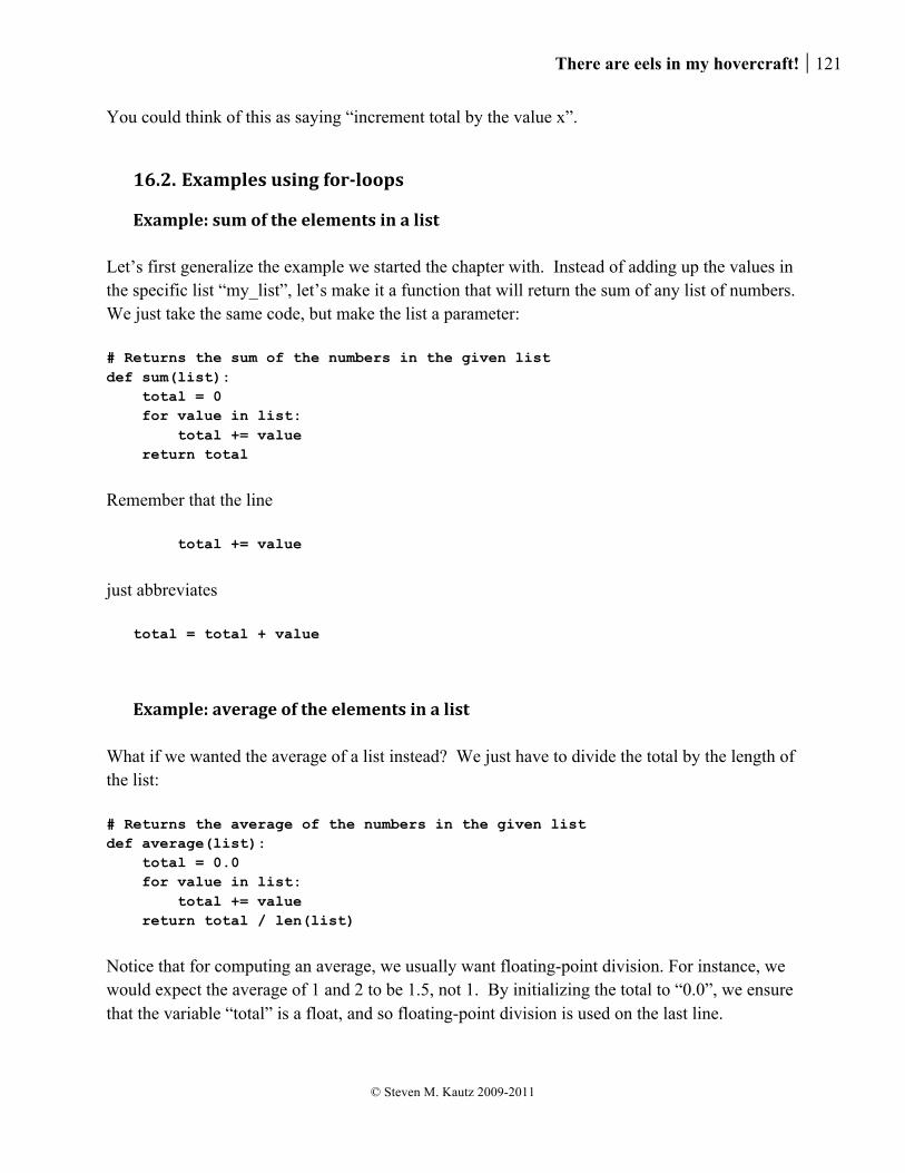
There are eels in my hovercraft! 121
© Steven M. Kautz 2009-2011
You could think of this as saying “increment total by the value x”.
16.2. Examples using for-‐loops
Example: sum of the elements in a list Let’s first generalize the example we started the chapter with. Instead of adding up the values in the specific list “my_list”, let’s make it a function that will return the sum of any list of numbers. We just take the same code, but make the list a parameter: # Returns the sum of the numbers in the given list def sum(list): total = 0 for value in list: total += value return total
Remember that the line total += value
just abbreviates
total = total + value
Example: average of the elements in a list What if we wanted the average of a list instead? We just have to divide the total by the length of the list: # Returns the average of the numbers in the given list def average(list): total = 0.0 for value in list: total += value return total / len(list)
Notice that for computing an average, we usually want floating-point division. For instance, we would expect the average of 1 and 2 to be 1.5, not 1. By initializing the total to “0.0”, we ensure that the variable “total” is a float, and so floating-point division is used on the last line.
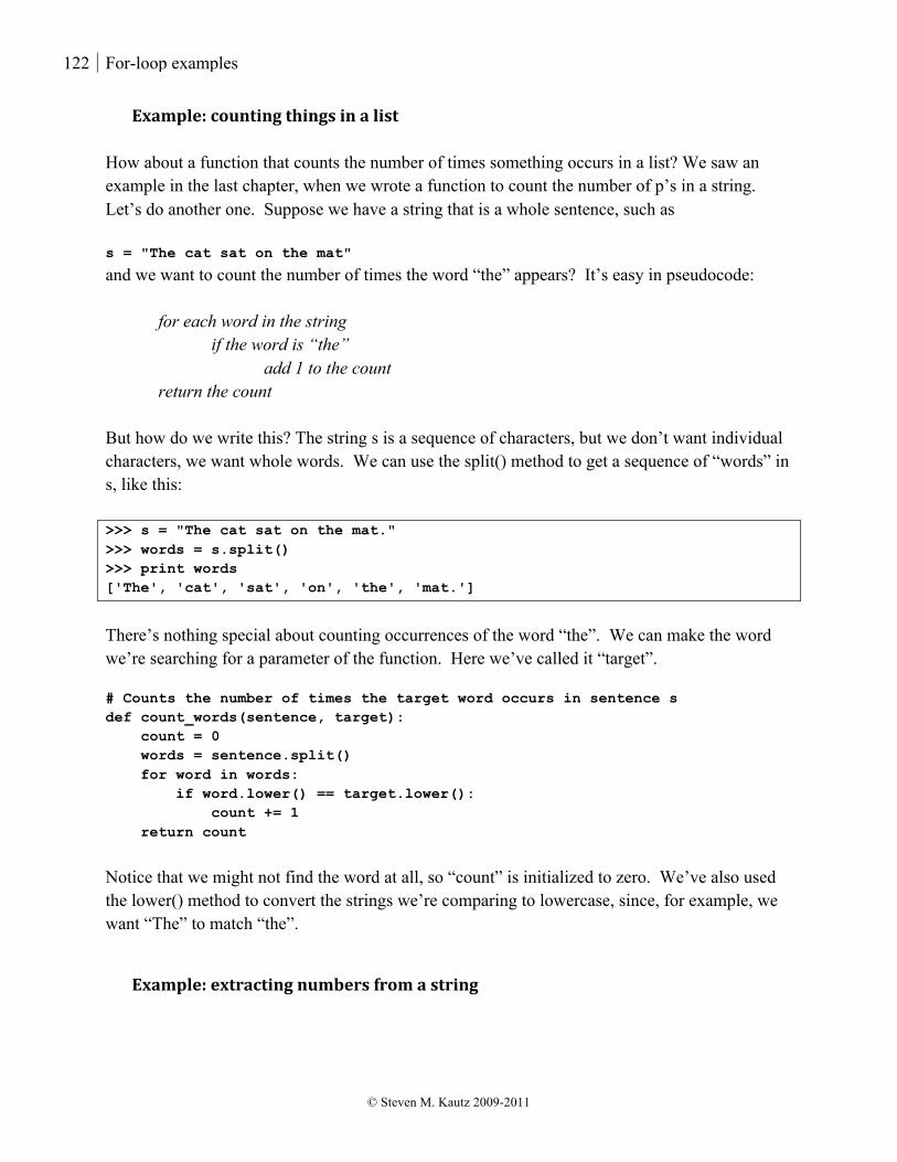
122 For-loop examples
© Steven M. Kautz 2009-2011
Example: counting things in a list How about a function that counts the number of times something occurs in a list? We saw an example in the last chapter, when we wrote a function to count the number of p’s in a string. Let’s do another one. Suppose we have a string that is a whole sentence, such as s = "The cat sat on the mat"
and we want to count the number of times the word “the” appears? It’s easy in pseudocode:
for each word in the string if the word is “the” add 1 to the count return the count
But how do we write this? The string s is a sequence of characters, but we don’t want individual characters, we want whole words. We can use the split() method to get a sequence of “words” in s, like this: >>> s = "The cat sat on the mat." >>> words = s.split() >>> print words ['The', 'cat', 'sat', 'on', 'the', 'mat.']
There’s nothing special about counting occurrences of the word “the”. We can make the word we’re searching for a parameter of the function. Here we’ve called it “target”. # Counts the number of times the target word occurs in sentence s def count_words(sentence, target): count = 0 words = sentence.split() for word in words: if word.lower() == target.lower(): count += 1 return count
Notice that we might not find the word at all, so “count” is initialized to zero. We’ve also used the lower() method to convert the strings we’re comparing to lowercase, since, for example, we want “The” to match “the”.
Example: extracting numbers from a string

There are eels in my hovercraft! 123
© Steven M. Kautz 2009-2011
In applications involving text and files, you might find you have a list of numbers given as a single string like this. s = "10 20 30 40"
To process a list of numbers given this way, we first have to separate them into individual strings using the split() method. Then you can iterate over the individual strings in the list using a for-loop. Since the items in the list are strings, if we want to do arithmetic with them, we have to use the int() or float() function to convert them to numbers. For example, here is a function that takes a string of numbers, separated by spaces, and return their sum. # Returns the sum of the numbers in # the space-delimited string s def sum_string(s): total = 0 strings = s.split() for w in strings: value = int(w) total += value return total
Example: maximum value in a list You might remember a problem we discussed in the very first chapter: how to find the largest number in a list. We finally have the knowledge we need to write the Python code for our solution to that problem. Recall how we did it. We initially set a variable, “max” to be the first number in the list.
max = the first element of the list for each number x in the list if x is greater than max update max to have value x
Then the value of “max” at the end is the answer. # Returns the largest element in the given list def find_max(list): max = list[0] for x in list: if x > max: max = x return max
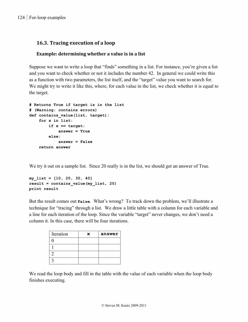
124 For-loop examples
© Steven M. Kautz 2009-2011
16.3. Tracing execution of a loop
Example: determining whether a value is in a list Suppose we want to write a loop that “finds” something in a list. For instance, you’re given a list and you want to check whether or not it includes the number 42. In general we could write this as a function with two parameters, the list itself, and the “target” value you want to search for. We might try to write it like this, where, for each value in the list, we check whether it is equal to the target. # Returns True if target is in the list # (Warning: contains errors) def contains_value(list, target): for x in list: if x == target: answer = True else: answer = False return answer
We try it out on a sample list. Since 20 really is in the list, we should get an answer of True. my_list = [10, 20, 30, 40] result = contains_value(my_list, 20) print result
But the result comes out False. What’s wrong? To track down the problem, we’ll illustrate a technique for “tracing” through a list. We draw a little table with a column for each variable and a line for each iteration of the loop. Since the variable “target” never changes, we don’t need a column it. In this case, there will be four iterations.
Iteration x answer 0 1 2 3
We read the loop body and fill in the table with the value of each variable when the loop body finishes executing.

There are eels in my hovercraft! 125
© Steven M. Kautz 2009-2011
for x in list: if x == target: answer = True else: answer = False
In the first iteration, x is 10. Since 10 isn’t equal to the target value 20, the answer is set to False.
Iteration x answer 0 10 False 1 2 3
Now, the loop body executes again with x holding the next value in the list, in this case 20. Since 20 is equal to the target, answer is set to True.
Iteration x answer 0 10 False 1 20 True 2 3
So far so good. But now the loop body executes again with x equal to 30. 30 isn’t equal to 20, so answer is set to False again.
Iteration x answer 0 10 False 1 20 True 2 30 False 3
The same thing happens in the last iteration when x is 40.
Iteration x answer 0 10 False 1 20 True 2 30 False
Loop body
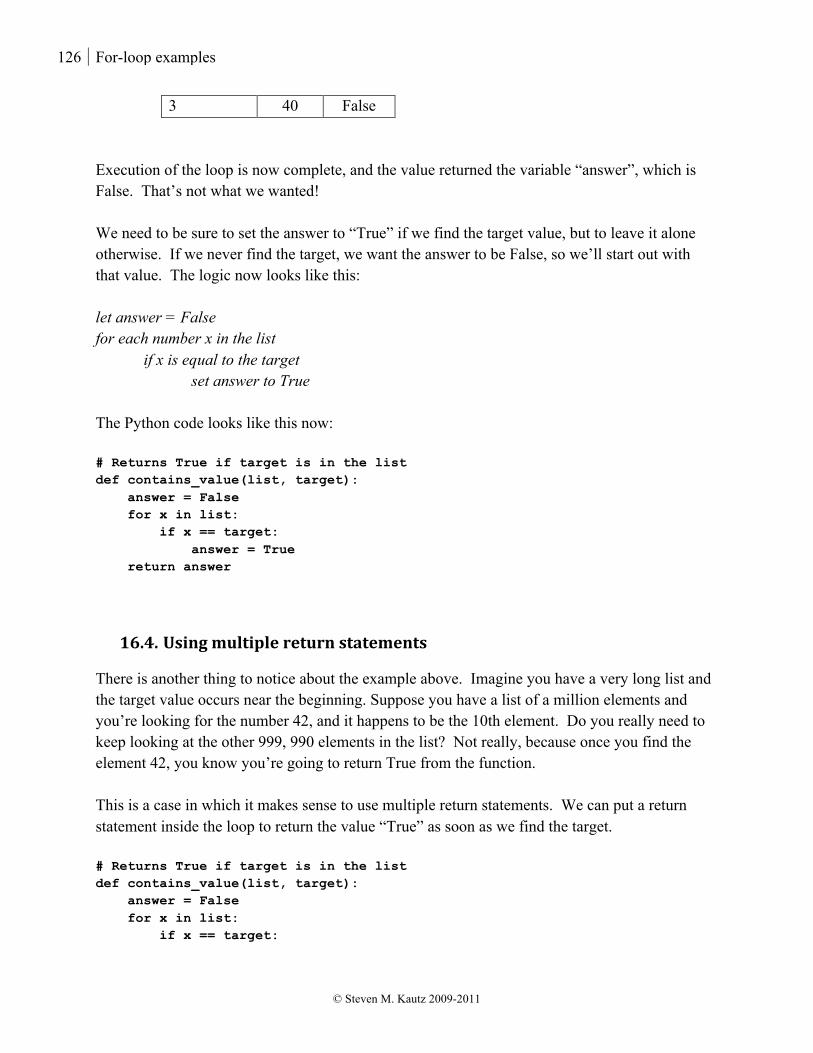
126 For-loop examples
© Steven M. Kautz 2009-2011
3 40 False Execution of the loop is now complete, and the value returned the variable “answer”, which is False. That’s not what we wanted! We need to be sure to set the answer to “True” if we find the target value, but to leave it alone otherwise. If we never find the target, we want the answer to be False, so we’ll start out with that value. The logic now looks like this: let answer = False for each number x in the list if x is equal to the target set answer to True The Python code looks like this now: # Returns True if target is in the list def contains_value(list, target): answer = False for x in list: if x == target: answer = True return answer
16.4. Using multiple return statements
There is another thing to notice about the example above. Imagine you have a very long list and the target value occurs near the beginning. Suppose you have a list of a million elements and you’re looking for the number 42, and it happens to be the 10th element. Do you really need to keep looking at the other 999, 990 elements in the list? Not really, because once you find the element 42, you know you’re going to return True from the function. This is a case in which it makes sense to use multiple return statements. We can put a return statement inside the loop to return the value “True” as soon as we find the target. # Returns True if target is in the list def contains_value(list, target): answer = False for x in list: if x == target:

There are eels in my hovercraft! 127
© Steven M. Kautz 2009-2011
return True # this statement only gets executed if we never find the target return False
Remember it is possible that we might examine every element of the list and not find the target. In that case, the loop completes all its iterations and we continue to the next statement after the loop. In this example, we just need to return a value of False. This idiom of putting a return statement in a loop is commonly used for loops that are “searching” for something, since it makes sense to return as soon as it is “found”.
Example: determining whether a number is prime Here’s another example. Let’s write a function that determines whether a given number is “prime”. Recall that a positive number if prime if it is not divisible by any number except 1 and itself. For example, 7 is prime, but 6 is not prime because it is divisible by 2. answer = True for each number d between 2 and n – 1 if n is divisible by d answer = False If we don’t find a number d that divides evenly into n, then the answer is True, so we start out with the answer equal to True. And if we do find a divisor of n, we can immediately return True. # Returns True if n is prime, False otherwise def is_prime(n): for d in range(2, n): if n % d == 0: return False return True
16.5. Tables and nested loops
Example: a table of square roots A common application of loops is to generate a table of values. For example, we could make a table of square roots of numbers up to 10. In pseudocode,
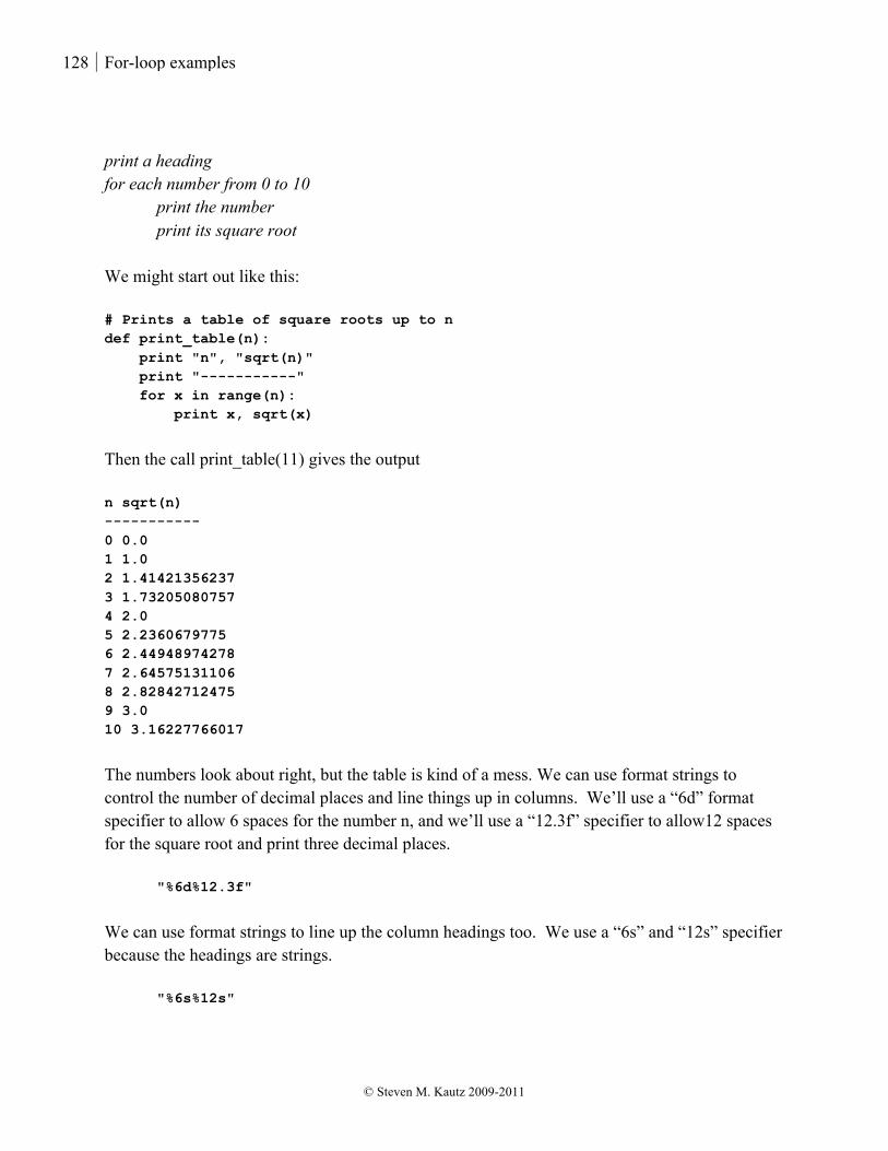
128 For-loop examples
© Steven M. Kautz 2009-2011
print a heading for each number from 0 to 10 print the number print its square root We might start out like this: # Prints a table of square roots up to n def print_table(n): print "n", "sqrt(n)" print "-----------" for x in range(n): print x, sqrt(x)
Then the call print_table(11) gives the output n sqrt(n) ----------- 0 0.0 1 1.0 2 1.41421356237 3 1.73205080757 4 2.0 5 2.2360679775 6 2.44948974278 7 2.64575131106 8 2.82842712475 9 3.0 10 3.16227766017
The numbers look about right, but the table is kind of a mess. We can use format strings to control the number of decimal places and line things up in columns. We’ll use a “6d” format specifier to allow 6 spaces for the number n, and we’ll use a “12.3f” specifier to allow12 spaces for the square root and print three decimal places.
"%6d%12.3f"
We can use format strings to line up the column headings too. We use a “6s” and “12s” specifier because the headings are strings.
"%6s%12s"

There are eels in my hovercraft! 129
© Steven M. Kautz 2009-2011
Remember that the actual values to be printed are listed in parentheses after the format string and a percent symbol. Here’s what the code looks like: # Prints a table of square roots up to n def print_table(n): print "%6s%12s" % ("n", "sqrt(n)") print "%6s%12s" % ("---", "-------") for x in range(n): print "%6d%12.3f" % (x, sqrt(x))
Now the output looks like this: n sqrt(n) --- ------- 0 0.000 1 1.000 2 1.414 3 1.732 4 2.000 5 2.236 6 2.449 7 2.646 8 2.828 9 3.000 10 3.162
Example: a multiplication table The body of a for-loop can include any statements. In particular, the body of a loop can include another loop. Why would you ever want to do that? As an example, let’s write a function that prints a multiplication table up to n times n, where n is a parameter. For instance, if n is 4, we would like to see output that looks like this. 1 2 3 4 2 4 6 8 3 6 9 12 4 8 12 16
The nature of printing output is that we have to do it row by row, so we might start out thinking like this: for each row r from 1 through n print the r-th row of the table

130 For-loop examples
© Steven M. Kautz 2009-2011
But what does “print the r-th row” mean? For example, look at the third row above. We need to print the value 1 times 3, 2 times 3, 3 times 3, and 4 times 3. In other words, given a row number r, we want something like this: for each column c from 1 through n print the number r * c So we put the pieces together. for each row r from 1 through n for each column c from 1 through n print the number r * c Can we write this in Python? Our first attempt looks just like the pseudocode. def print_table(n): for r in range(1, n + 1): for c in range(1, n + 1): print r * c
But we try a call to print_table(10) and it doesn’t make a table at all. All the values are printed on a different line. 1 2 3 4 5 ...
We can put a comma after the print statement to keep it from going to the next line. But then we have the opposite problem. Now everything is on one line! 1 2 3 4 5 6 7 8 9 10 2 4 6 8 10 12 14 16 18 20 3 6 9 12 15 18 21 24 27 30...
After each row is completed, we need to add an empty print statement to go to the next line. def print_table(n): for r in range(1, n + 1): for c in range(1, n + 1): print r * c, print

There are eels in my hovercraft! 131
© Steven M. Kautz 2009-2011
Now the call print_table(10) gives us this output: 1 2 3 4 5 6 7 8 9 10 2 4 6 8 10 12 14 16 18 20 3 6 9 12 15 18 21 24 27 30 4 8 12 16 20 24 28 32 36 40 5 10 15 20 25 30 35 40 45 50 6 12 18 24 30 36 42 48 54 60 7 14 21 28 35 42 49 56 63 70 8 16 24 32 40 48 56 64 72 80 9 18 27 36 45 54 63 72 81 90 10 20 30 40 50 60 70 80 90 100
That’s much better. Next, we want to try to line things up in columns. We can’t use a single format string for each line, because we don’t know in advance how many values will be on a given line. But we can still use a format string to print the individual values using a fixed number of spaces. Here we’ll use a “4d” specifier to allow 4 spaces for each value. def print_table(n): for r in range(1, n + 1): for c in range(1, n + 1): print "%4d" % (r * c), print
This code now gives us this output: 1 2 3 4 5 6 7 8 9 10 2 4 6 8 10 12 14 16 18 20 3 6 9 12 15 18 21 24 27 30 4 8 12 16 20 24 28 32 36 40 5 10 15 20 25 30 35 40 45 50 6 12 18 24 30 36 42 48 54 60 7 14 21 28 35 42 49 56 63 70 8 16 24 32 40 48 56 64 72 80 9 18 27 36 45 54 63 72 81 90 10 20 30 40 50 60 70 80 90 100
132 For-loop examples
© Steven M. Kautz 2009-2011

There are eels in my hovercraft! 133
© Steven M. Kautz 2009-2011
17. While-‐loops 17.1. Beat until smooth
In the last two chapters we have been learning about for-loops. A for-loop is the simplest solution when you start out with a fixed sequence, and you want to perform some action once for each item.
for each cupcake put on frosting and sprinkles
You always know the number of iterations in advance, or at least the maximum number of iterations, since you could exit the loop early. But there are situations when you don’t start out with a known sequence of items to act upon, and you don’t know in advance how many times something is going to happen. For example, the directions for making the cupcakes might have said something like
add two eggs and beat until smooth So, how much are we supposed to beat? As long as it is still lumpy, we have to beat it some more. You have probably experienced similar situations.
drive around the block until you find a parking place keep practicing until you can play the whole piece without mistakes
We can describe activities like this a bit more precisely using the word “while”.
while we haven’t found a parking place drive around the block again while there are mistakes practice the piece again while there are lumps in the batter beat it some more
In programming, situations like this call for a more general type of loop, called a while-loop. In Python, a while-loop is written with the while keyword:

134 While-loops
© Steven M. Kautz 2009-2011
while condition: statement- block
As with a for-loop, the statement block is known as the loop body. The way it works is really simple. If the condition is true, the loop body gets executed. After the loop body executes, we go back and re-check the condition. If the condition is still true, the loop body is executed again. And so on. And so on. And so on.
condition?
False
True
execute statements in loop body
As a simple example to start with, let’s write a loop that prints the characters in a string one at a time. We did this already using a for-loop. It was easy. We basically just said, “For each character in the string, print it.”
word = "Steve" for ch in word: print ch
To do the same thing with a while-loop, we have to work a little bit harder. We have to keep track of the index for the next character, and increment the index ourselves.
index = 0 while index < len(word): ch = word[index] print ch index +=1

There are eels in my hovercraft! 135
© Steven M. Kautz 2009-2011
To make sure we understand what’s going on here, let’s trace through this code using a table as we did in the last unit. Before entering the loop, the initial value of “index” is zero, and the variable “ch” is undefined.
index ch Output Initial values
0 ?
Now, we check the condition. The length of “Steve” is 5. Is index less than 5? The answer is yes, so we enter the loop body. “ch” gets the character at index 0, which is “S”, and then index is incremented by 1. We write down the values of the variables at the end of the loop body, and we’ll also show the output in the table.
index ch Output Initial values
0 ?
Iteration 0 1 “S” S Now, we go back and check the condition again. “index” is 1. Is 1 less than 5? Yes, so we enter the loop body. “ch” gets the character at index 1, which is “t”, and then index is incremented by 1.
index ch Output Initial values
0 ?
Iteration 0 1 “S” S Iteration 1 2 “t” t
Check the condition again. Index is still less than 5, so we execute the loop body again.
index ch Output Initial values
0 ?
Iteration 0 1 “S” S Iteration 1 2 “t” t Iteration 2 3 “e” e
Check the condition, and execute the loop body again.
index ch Output
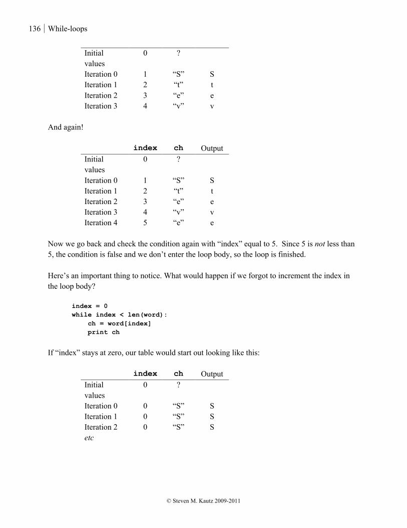
136 While-loops
© Steven M. Kautz 2009-2011
Initial values
0 ?
Iteration 0 1 “S” S Iteration 1 2 “t” t Iteration 2 3 “e” e Iteration 3 4 “v” v
And again!
index ch Output Initial values
0 ?
Iteration 0 1 “S” S Iteration 1 2 “t” t Iteration 2 3 “e” e Iteration 3 4 “v” v Iteration 4 5 “e” e
Now we go back and check the condition again with “index” equal to 5. Since 5 is not less than 5, the condition is false and we don’t enter the loop body, so the loop is finished. Here’s an important thing to notice. What would happen if we forgot to increment the index in the loop body?
index = 0 while index < len(word): ch = word[index] print ch
If “index” stays at zero, our table would start out looking like this:
index ch Output Initial values
0 ?
Iteration 0 0 “S” S Iteration 1 0 “S” S Iteration 2 0 “S” S etc

There are eels in my hovercraft! 137
© Steven M. Kautz 2009-2011
The condition “index is less than the length of ‘Steve’” is always true, so the loop body keeps executing over and over again, printing the character “S”. Forever! This is called an infinite loop. Sometimes we write infinite loops on purpose, for applications that are supposed to keep running all the time, like web servers and telephone switches. But sometimes we get infinite loops from programming errors. One thing you should be sure to know is: how do you stop an infinite loop? In most environments, the key combination “Control-C” will work. It’s also possible for the opposite to happen. What if we had this, where the inequality is accidentally reversed.
index = 0 while index > len(word): ch = word[index] print ch index +=1
The condition starts out false, so the loop body will never execute, not even once. You can see that while-loops are a bit more difficult to write than for-loops. So why would we ever want to use them? We need while-loops for situations in which we don’t have a fixed list of items to iterate over or we don’t know the number of iterations in advance.
17.2. Examples of while-‐loops
Remember that in the last chapter, we wrote a for-loop to find the sum of a sequence of numbers. What if instead of having a known sequence, the numbers were being entered one at a time from the keyboard? We don’t necessarily know in advance how many values there will be. Instead, let’s assume that the user can enter a “q” to indicate that there are no more values to enter. We’ll just print the total when the user is done. Logically we want something like this
get the first value from the user while the value entered is not “q” add the value to the total get the next value from the user print the total
total = 0
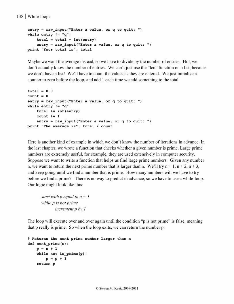
138 While-loops
© Steven M. Kautz 2009-2011
entry = raw_input("Enter a value, or q to quit: ") while entry != "q": total = total + int(entry) entry = raw_input("Enter a value, or q to quit: ") print "Your total is", total
Maybe we want the average instead, so we have to divide by the number of entries. Hm, we don’t actually know the number of entries. We can’t just use the “len” function on a list, because we don’t have a list! We’ll have to count the values as they are entered. We just initialize a counter to zero before the loop, and add 1 each time we add something to the total. total = 0.0 count = 0 entry = raw_input("Enter a value, or q to quit: ") while entry != "q": total += int(entry) count += 1 entry = raw_input("Enter a value, or q to quit: ") print "The average is", total / count
Here is another kind of example in which we don’t know the number of iterations in advance. In the last chapter, we wrote a function that checks whether a given number is prime. Large prime numbers are extremely useful, for example, they are used extensively in computer security. Suppose we want to write a function that helps us find large prime numbers. Given any number n, we want to return the next prime number that is larger than n. We’ll try n + 1, n + 2, n + 3, and keep going until we find a number that is prime. How many numbers will we have to try before we find a prime? There is no way to predict in advance, so we have to use a while-loop. Our logic might look like this:
start with p equal to n + 1 while p is not prime increment p by 1
The loop will execute over and over again until the condition “p is not prime” is false, meaning that p really is prime. So when the loop exits, we can return the number p. # Returns the next prime number larger than n def next_prime(n): p = n + 1 while not is_prime(p): p = p + 1 return p
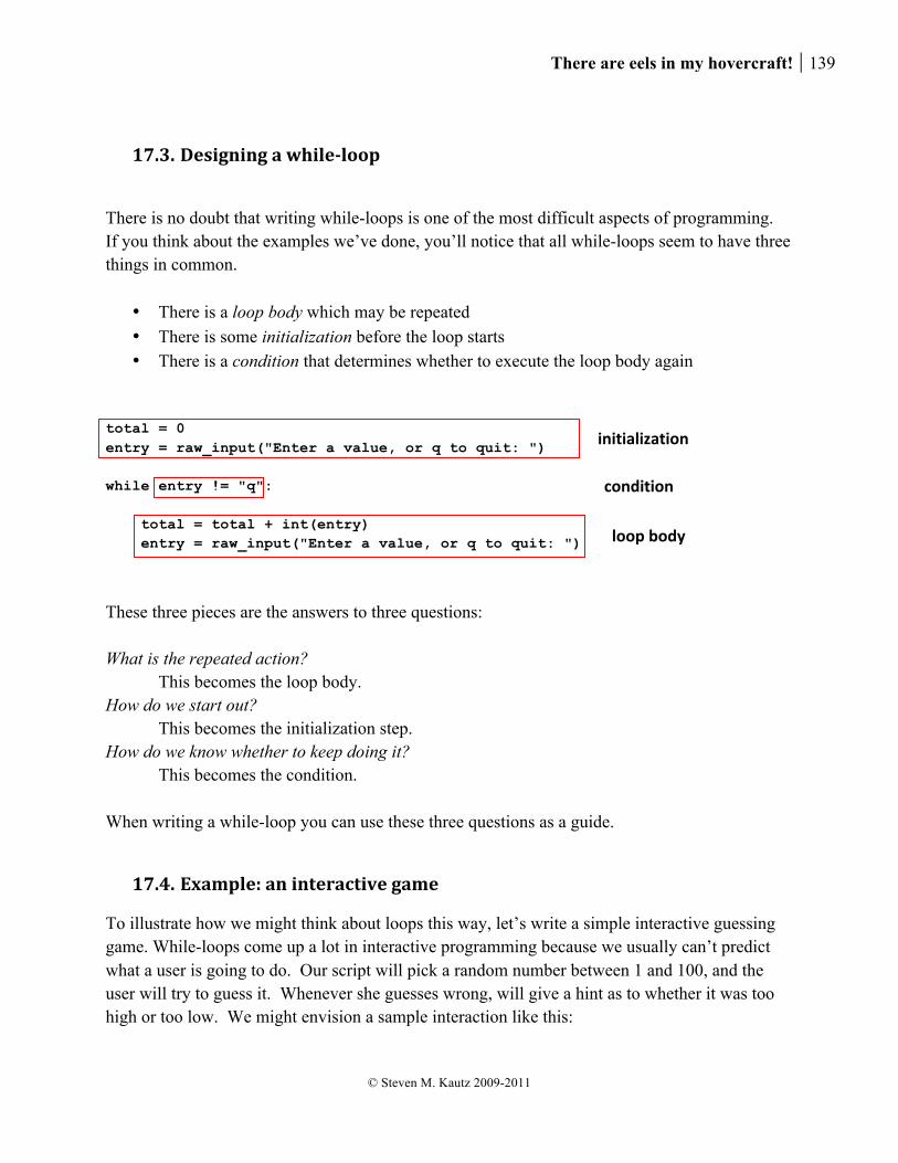
There are eels in my hovercraft! 139
© Steven M. Kautz 2009-2011
17.3. Designing a while-‐loop
There is no doubt that writing while-loops is one of the most difficult aspects of programming. If you think about the examples we’ve done, you’ll notice that all while-loops seem to have three things in common.
• There is a loop body which may be repeated • There is some initialization before the loop starts • There is a condition that determines whether to execute the loop body again
total = 0 entry = raw_input("Enter a value, or q to quit: ") while entry != "q": total = total + int(entry) entry = raw_input("Enter a value, or q to quit: ")
These three pieces are the answers to three questions: What is the repeated action? This becomes the loop body. How do we start out? This becomes the initialization step. How do we know whether to keep doing it? This becomes the condition. When writing a while-loop you can use these three questions as a guide.
17.4. Example: an interactive game
To illustrate how we might think about loops this way, let’s write a simple interactive guessing game. While-loops come up a lot in interactive programming because we usually can’t predict what a user is going to do. Our script will pick a random number between 1 and 100, and the user will try to guess it. Whenever she guesses wrong, will give a hint as to whether it was too high or too low. We might envision a sample interaction like this:
loop body
initialization
condition
140 While-loops
© Steven M. Kautz 2009-2011
Try to guess a number between 1 and 100 What's your first guess? 50 Too low! What's your next guess? 75 Too high! What's your next guess? 60 Too low! What's your next guess? 70 That's it!
How do we pick a number at random? In reality, computers can’t do anything that truly depends on chance, like flipping coins or rolling dice. However, there are ways to generate values that appear to be random in the sense that they are unpredictable and well-distributed over a range of values. In Python, we can use a function called randint() from the module called “random”. Let’s try it out in the shell: >>> from random import randint >>> randint(1, 10) 2 >>> randint(1, 10) 10 >>> randint(1, 10) 4
The call randint(a, b) generates a random value between a and b, inclusive. When you try it, of course, you’ll probably see different numbers. Let’s think about the loop for the guessing game by asking the three questions. Step 1: What is the repeated action? Check whether the guess is too low or too high, and print a message. Then, get the user’s next guess. Step 2: How do we start out? We need to generate the secret number, and we need to get the user’s first guess. Step 3: How do we know whether to keep doing it? The user’s guess isn’t the secret number.
There are eels in my hovercraft! 141
© Steven M. Kautz 2009-2011
For step 1, if we define a variable “secret” to represent the secret number, and a variable “guess” to represent the user’s guess, the code for the repeated action could be written like this. The repeated action will be the body of a while-loop. We’ll write the loop body, and worry about the condition later. while ? : if guess < secret: print "Too low!" else: print "Too high!" guess = input("What's your next guess? ")
For step 2, we can use the randint() function to initialize the secret number, and then read the user’s first guess. secret = randint(1, 100) print "Try to guess a number between 1 and 100" guess = input("What's your first guess? ")
For step 3, we just need a condition that says that “guess” isn’t equal to “secret”: while guess != secret:
We’ll put the code into a function play_game. We need one additional line after the loop, to tell the user when she is successful. from random import randint # Plays one round of a number-guessing game def play_game(): secret = randint(1, 100) print "Try to guess a number between 1 and 100" guess = input("What's your first guess? ") while guess != secret: if guess < secret: print "Too low!" else: print "Too high!" guess = input("What's your next guess? ") print "That's it!"
We might add a user interface for this function so that the user can choose whether to play again, or quit. One way to do this is to provide a “menu” of choices, which might look like this:

142 While-loops
© Steven M. Kautz 2009-2011
p) Play the guessing game q) Quit
We can generate the menu with a simple function: def menu(): print " p) Play the guessing game" print " q) Quit"
Since we can’t predict in advance how many times the user wants to play the game, we need a while loop. We’ll write the loop using asking the usual three questions: Step 1: What is the repeated action? Perform the user’s choice, display the menu, and allow the user to select an option. Step 2: How do we start out? Display the menu and allow the user to select an option. Step 3: How do we know whether to keep doing it? We keep doing it as long as the user doesn’t enter a “q”. For step 1, we have to check what the user entered and perform the operation. Since there is only one choice besides “quit”, we are really just checking whether the entry is valid. If the user really does enter a “p”, we call the play_game function to play one round. The repeated actions become the body of the loop. while ? : if entry == "p": play_game() else: print "Please select p or q" menu() entry = raw_input("Enter your choice: ")
For step 2, we need to display the menu and get the user’s first selection. print "Welcome to the guessing game" menu() entry = raw_input("Enter your choice: ")

There are eels in my hovercraft! 143
© Steven M. Kautz 2009-2011
while ? : if entry == "p": play_game() else: print "Please select p or q" menu() entry = raw_input("Enter your choice: ")
For step 3, the loop condition simply checks that the entry is not a “q”. while entry != "q":
When the pieces are put together the whole script looks like this: # Main loop for a number-guessing game def run_guessing_game(): print "Welcome to the guessing game" menu() entry = raw_input("Enter your choice: ") while entry != "q": if entry == "p": play_game() else: print "Please select p or q" menu() entry = raw_input("Enter your choice: ") print "Thanks for playing. Bye!"
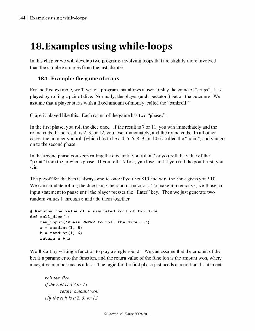
144 Examples using while-loops
© Steven M. Kautz 2009-2011
18. Examples using while-‐loops In this chapter we will develop two programs involving loops that are slightly more involved than the simple examples from the last chapter.
18.1. Example: the game of craps
For the first example, we’ll write a program that allows a user to play the game of “craps”. It is played by rolling a pair of dice. Normally, the player (and spectators) bet on the outcome. We assume that a player starts with a fixed amount of money, called the “bankroll.” Craps is played like this. Each round of the game has two “phases”:
In the first phase, you roll the dice once. If the result is 7 or 11, you win immediately and the round ends. If the result is 2, 3, or 12, you lose immediately, and the round ends. In all other cases the number you roll (which has to be a 4, 5, 6, 8, 9, or 10) is called the “point”, and you go on to the second phase. In the second phase you keep rolling the dice until you roll a 7 or you roll the value of the “point” from the previous phase. If you roll a 7 first, you lose, and if you roll the point first, you win The payoff for the bets is always one-to-one: if you bet $10 and win, the bank gives you $10. We can simulate rolling the dice using the randint function. To make it interactive, we’ll use an input statement to pause until the player presses the “Enter” key. Then we just generate two random values 1 through 6 and add them together # Returns the value of a simulated roll of two dice def roll_dice(): raw_input("Press ENTER to roll the dice...") a = randint(1, 6) b = randint(1, 6) return a + b
We’ll start by writing a function to play a single round. We can assume that the amount of the bet is a parameter to the function, and the return value of the function is the amount won, where a negative number means a loss. The logic for the first phase just needs a conditional statement.
roll the dice if the roll is a 7 or 11 return amount won elif the roll is a 2, 3, or 12
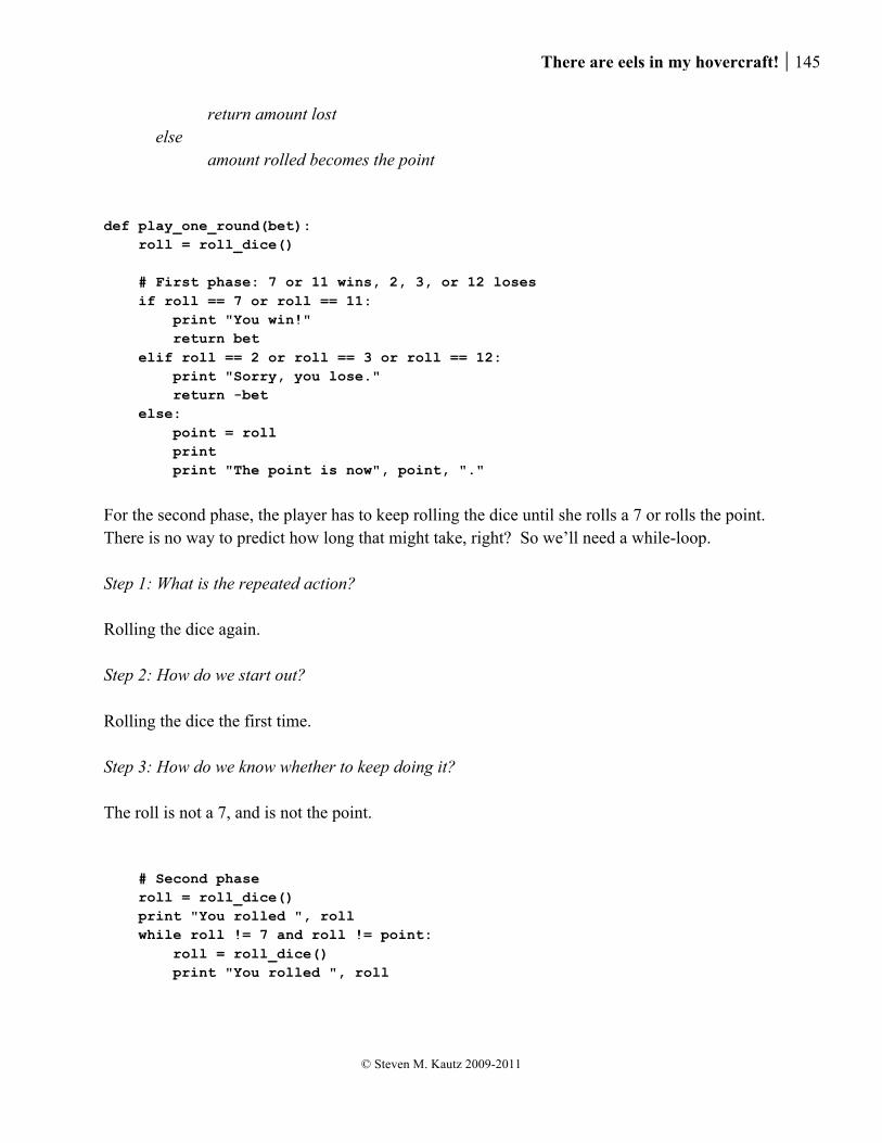
There are eels in my hovercraft! 145
© Steven M. Kautz 2009-2011
return amount lost else amount rolled becomes the point
def play_one_round(bet): roll = roll_dice() # First phase: 7 or 11 wins, 2, 3, or 12 loses if roll == 7 or roll == 11: print "You win!" return bet elif roll == 2 or roll == 3 or roll == 12: print "Sorry, you lose." return -bet else: point = roll print print "The point is now", point, "."
For the second phase, the player has to keep rolling the dice until she rolls a 7 or rolls the point. There is no way to predict how long that might take, right? So we’ll need a while-loop. Step 1: What is the repeated action? Rolling the dice again. Step 2: How do we start out? Rolling the dice the first time. Step 3: How do we know whether to keep doing it? The roll is not a 7, and is not the point. # Second phase roll = roll_dice() print "You rolled ", roll while roll != 7 and roll != point: roll = roll_dice() print "You rolled ", roll
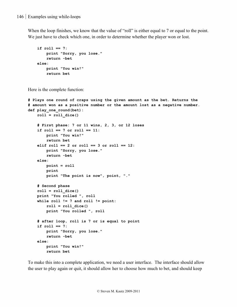
146 Examples using while-loops
© Steven M. Kautz 2009-2011
When the loop finishes, we know that the value of “roll” is either equal to 7 or equal to the point. We just have to check which one, in order to determine whether the player won or lost. if roll == 7: print "Sorry, you lose." return -bet else: print "You win!" return bet
Here is the complete function: # Plays one round of craps using the given amount as the bet. Returns the # amount won as a positive number or the amount lost as a negative number. def play_one_round(bet): roll = roll_dice() # First phase: 7 or 11 wins, 2, 3, or 12 loses if roll == 7 or roll == 11: print "You win!" return bet elif roll == 2 or roll == 3 or roll == 12: print "Sorry, you lose." return -bet else: point = roll print print "The point is now", point, "." # Second phase roll = roll_dice() print "You rolled ", roll while roll != 7 and roll != point: roll = roll_dice() print "You rolled ", roll # after loop, roll is 7 or is equal to point if roll == 7: print "Sorry, you lose." return -bet else: print "You win!" return bet
To make this into a complete application, we need a user interface. The interface should allow the user to play again or quit, it should allow her to choose how much to bet, and should keep
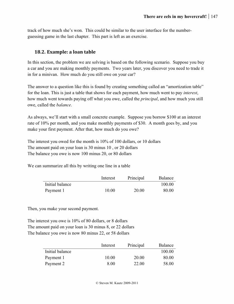
There are eels in my hovercraft! 147
© Steven M. Kautz 2009-2011
track of how much she’s won. This could be similar to the user interface for the number-guessing game in the last chapter. This part is left as an exercise.
18.2. Example: a loan table
In this section, the problem we are solving is based on the following scenario. Suppose you buy a car and you are making monthly payments. Two years later, you discover you need to trade it in for a minivan. How much do you still owe on your car? The answer to a question like this is found by creating something called an “amortization table” for the loan. This is just a table that shows for each payment, how much went to pay interest, how much went towards paying off what you owe, called the principal, and how much you still owe, called the balance. As always, we’ll start with a small concrete example. Suppose you borrow $100 at an interest rate of 10% per month, and you make monthly payments of $30. A month goes by, and you make your first payment. After that, how much do you owe? The interest you owed for the month is 10% of 100 dollars, or 10 dollars The amount paid on your loan is 30 minus 10 , or 20 dollars The balance you owe is now 100 minus 20, or 80 dollars We can summarize all this by writing one line in a table
Interest Principal Balance Initial balance 100.00 Payment 1 10.00 20.00 80.00
Then, you make your second payment. The interest you owe is 10% of 80 dollars, or 8 dollars The amount paid on your loan is 30 minus 8, or 22 dollars The balance you owe is now 80 minus 22, or 58 dollars
Interest Principal Balance Initial balance 100.00 Payment 1 10.00 20.00 80.00 Payment 2 8.00 22.00 58.00
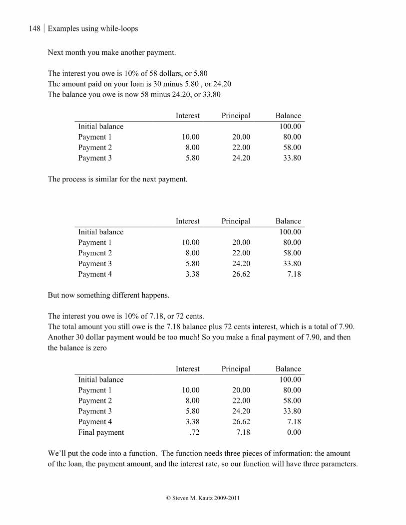
148 Examples using while-loops
© Steven M. Kautz 2009-2011
Next month you make another payment. The interest you owe is 10% of 58 dollars, or 5.80 The amount paid on your loan is 30 minus 5.80 , or 24.20 The balance you owe is now 58 minus 24.20, or 33.80
Interest Principal Balance Initial balance 100.00 Payment 1 10.00 20.00 80.00 Payment 2 8.00 22.00 58.00 Payment 3 5.80 24.20 33.80
The process is similar for the next payment.
Interest Principal Balance Initial balance 100.00 Payment 1 10.00 20.00 80.00 Payment 2 8.00 22.00 58.00 Payment 3 5.80 24.20 33.80 Payment 4 3.38 26.62 7.18
But now something different happens. The interest you owe is 10% of 7.18, or 72 cents. The total amount you still owe is the 7.18 balance plus 72 cents interest, which is a total of 7.90. Another 30 dollar payment would be too much! So you make a final payment of 7.90, and then the balance is zero
Interest Principal Balance Initial balance 100.00 Payment 1 10.00 20.00 80.00 Payment 2 8.00 22.00 58.00 Payment 3 5.80 24.20 33.80 Payment 4 3.38 26.62 7.18 Final payment .72 7.18 0.00
We’ll put the code into a function. The function needs three pieces of information: the amount of the loan, the payment amount, and the interest rate, so our function will have three parameters.
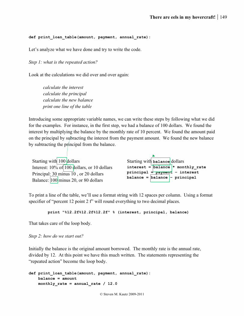
There are eels in my hovercraft! 149
© Steven M. Kautz 2009-2011
def print_loan_table(amount, payment, annual_rate):
Let’s analyze what we have done and try to write the code. Step 1: what is the repeated action? Look at the calculations we did over and over again:
calculate the interest calculate the principal calculate the new balance print one line of the table
Introducing some appropriate variable names, we can write these steps by following what we did for the examples. For instance, in the first step, we had a balance of 100 dollars. We found the interest by multiplying the balance by the monthly rate of 10 percent. We found the amount paid on the principal by subracting the interest from the payment amount. We found the new balance by subtracting the principal from the balance. To print a line of the table, we’ll use a format string with 12 spaces per column. Using a format specifier of “percent 12 point 2 f” will round everything to two decimal places. print "%12.2f%12.2f%12.2f" % (interest, principal, balance)
That takes care of the loop body. Step 2: how do we start out? Initially the balance is the original amount borrowed. The monthly rate is the annual rate, divided by 12. At this point we have this much written. The statements representing the “repeated action” become the loop body. def print_loan_table(amount, payment, annual_rate): balance = amount monthly_rate = annual_rate / 12.0
Starting with 100 dollars Interest: 10% of 100 dollars, or 10 dollars Principal: 30 minus 10 , or 20 dollars Balance: 100 minus 20, or 80 dollars
Starting with balance dollars interest = balance * monthly_rate principal = payment – interest balance = balance – principal
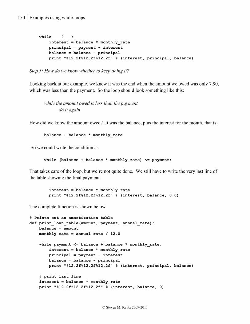
150 Examples using while-loops
© Steven M. Kautz 2009-2011
while ? : interest = balance * monthly_rate principal = payment - interest balance = balance - principal print "%12.2f%12.2f%12.2f" % (interest, principal, balance)
Step 3: How do we know whether to keep doing it? Looking back at our example, we knew it was the end when the amount we owed was only 7.90, which was less than the payment. So the loop should look something like this:
while the amount owed is less than the payment do it again
How did we know the amount owed? It was the balance, plus the interest for the month, that is:
balance + balance * monthly_rate
So we could write the condition as
while (balance + balance * monthly_rate) <= payment:
That takes care of the loop, but we’re not quite done. We still have to write the very last line of the table showing the final payment. interest = balance * monthly_rate print "%12.2f%12.2f%12.2f" % (interest, balance, 0.0)
The complete function is shown below. # Prints out an amortization table def print_loan_table(amount, payment, annual_rate): balance = amount monthly_rate = annual_rate / 12.0 while payment <= balance + balance * monthly_rate: interest = balance * monthly_rate principal = payment - interest balance = balance - principal print "%12.2f%12.2f%12.2f" % (interest, principal, balance) # print last line interest = balance * monthly_rate print "%12.2f%12.2f%12.2f" % (interest, balance, 0)

There are eels in my hovercraft! 151
© Steven M. Kautz 2009-2011

152 Reading text files
© Steven M. Kautz 2009-2011
19. Reading text files Up to this point in the course, we have written short programs or games that process small amounts of data that a user can type at the keyboard. The information entered by the user is stored in variables that only exist during the time when the program is running. If there is a lot of data, it isn’t practical to re-enter it all every time you want to run the program. For example, what if you want the class average for a class with several hundred students, or you want to sort the membership list for a club with several thousand members. In most situations, the data is stored on your computer in some kind of file, and we need to be able to read the data from the file. We previously discussed the idea that all data has to be encoded somehow when it is stored or processed by a computer. There are many types of files that encode different types of data. You probably have files that contain pictures, music, Microsoft Word documents, and so on. The simplest kind of file is a text file. In a text file, each byte is a printable character or possibly a tab or newline. Text files are useful and easy to work with. In this chapter we will learn how to read data from text files.
19.1. Opening and reading a file
Working with files is different than working with ordinary variables, because a file is something that lives outside of the Python interpreter and is under the control of the operating system. In order to read a file’s contents within your script, the interpreter has to ask the operating system to go find it on the hard drive or other device to and prepare to read it. This is called “opening” the file. You open a file in Python using a built-in function called open(). The argument to open() is the name of the file to be opened. For example, suppose we have a file called “testfile.txt” and we create a script in the same directory called “filetest.py”, as shown. In this chapter we are going to assume that the file to be read is always in the same directory as the script that is opening the file. Later we will learn how to work around this restriction.

There are eels in my hovercraft! 153
© Steven M. Kautz 2009-2011
Let’s take a moment to examine what the script does. The line myfile = open("testfile.txt")
asks the operating system to find the file called “testfile.txt” and prepare to read it. The variable “myfile” is what we use to refer to the file within our script. The most basic operation on a file is to read it one line at a time, and to process the line somehow. We can read all the lines of a file with a for-loop. for line in myfile: print line, Each line is a string. In this case, all we’re doing to “process” the line is to print it. Notice the comma at the end of the print statement. The line itself includes a newline character at the end, so we have to tell the print statement not to insert another newline. The last line, myfile.close()
“closes” the file. The operating system will update the actual contents of the file on the hard drive or other device, and the file will be available for other applications to use. When we run the testfile script, we just see the contents of the file printed on the screen. This is a short text file. It has seven lines,
This is a short text file. It has seven lines, one of which is blank.
myfile = open("testfile.txt") for line in myfile: print line, myfile.close()
File: testfile.txt File: filetest.py
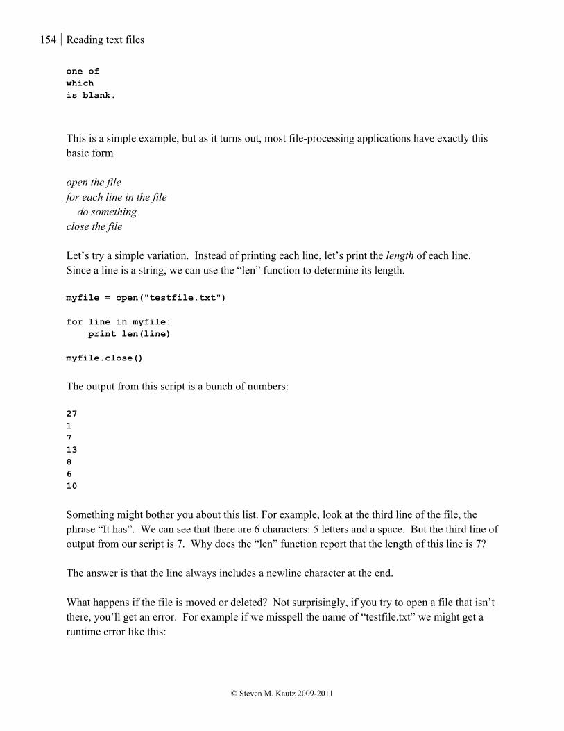
154 Reading text files
© Steven M. Kautz 2009-2011
one of which is blank.
This is a simple example, but as it turns out, most file-processing applications have exactly this basic form open the file for each line in the file do something close the file Let’s try a simple variation. Instead of printing each line, let’s print the length of each line. Since a line is a string, we can use the “len” function to determine its length. myfile = open("testfile.txt") for line in myfile: print len(line) myfile.close() The output from this script is a bunch of numbers: 27 1 7 13 8 6 10
Something might bother you about this list. For example, look at the third line of the file, the phrase “It has”. We can see that there are 6 characters: 5 letters and a space. But the third line of output from our script is 7. Why does the “len” function report that the length of this line is 7? The answer is that the line always includes a newline character at the end. What happens if the file is moved or deleted? Not surprisingly, if you try to open a file that isn’t there, you’ll get an error. For example if we misspell the name of “testfile.txt” we might get a runtime error like this:
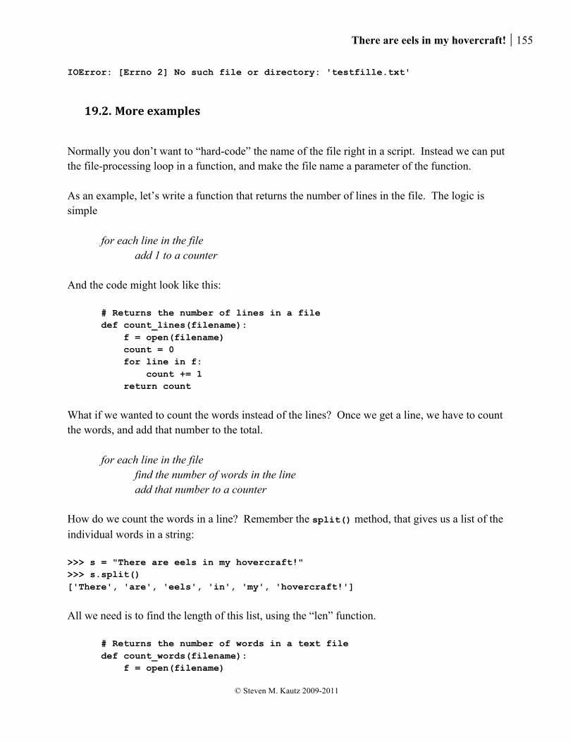
There are eels in my hovercraft! 155
© Steven M. Kautz 2009-2011
IOError: [Errno 2] No such file or directory: 'testfille.txt'
19.2. More examples
Normally you don’t want to “hard-code” the name of the file right in a script. Instead we can put the file-processing loop in a function, and make the file name a parameter of the function. As an example, let’s write a function that returns the number of lines in the file. The logic is simple
for each line in the file add 1 to a counter
And the code might look like this:
# Returns the number of lines in a file def count_lines(filename): f = open(filename) count = 0 for line in f: count += 1 return count
What if we wanted to count the words instead of the lines? Once we get a line, we have to count the words, and add that number to the total.
for each line in the file find the number of words in the line add that number to a counter
How do we count the words in a line? Remember the split() method, that gives us a list of the individual words in a string: >>> s = "There are eels in my hovercraft!" >>> s.split() ['There', 'are', 'eels', 'in', 'my', 'hovercraft!']
All we need is to find the length of this list, using the “len” function.
# Returns the number of words in a text file def count_words(filename): f = open(filename)

156 Reading text files
© Steven M. Kautz 2009-2011
count = 0 for line in f: word_count = len(line.split()) count += word_count return count
19.3. Files with numbers
Suppose that a text file contains names and quiz scores, in the following format.
Hermione Granger 10 10 10 10 10 10 Fred Weasley 4 5 6 Harry Potter 8 9 8 10 3 10
We want to write a function that will read a file like this and print the average score for each person, for example,
Hermione Granger 100.0 Fred Weasley 25.0 Harry Potter 80.0
We’ll need to know the name of the file and the total points for the quizzes (60, in this example) so the function definition would look like this:
def get_averages(filename, possible_points):
We’ll start with the basic file-processing loop:
open the file for each line in the file do something close the file
So we can write a “skeleton” of the function pretty easily:
def get_averages(filename, possible_points): f = open(filename) for line in f: # do interesting stuff here f.close()
Now, what do we need to do for each line?
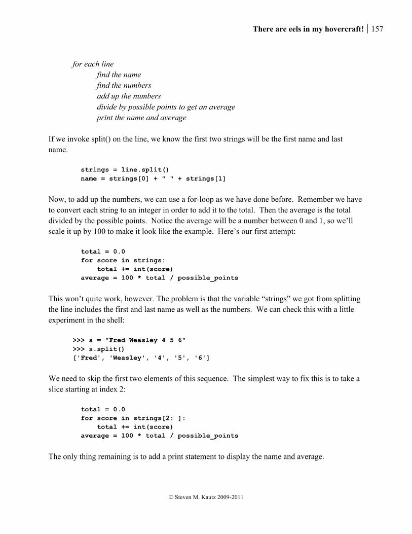
There are eels in my hovercraft! 157
© Steven M. Kautz 2009-2011
for each line find the name find the numbers add up the numbers divide by possible points to get an average print the name and average
If we invoke split() on the line, we know the first two strings will be the first name and last name. strings = line.split() name = strings[0] + " " + strings[1]
Now, to add up the numbers, we can use a for-loop as we have done before. Remember we have to convert each string to an integer in order to add it to the total. Then the average is the total divided by the possible points. Notice the average will be a number between 0 and 1, so we’ll scale it up by 100 to make it look like the example. Here’s our first attempt: total = 0.0 for score in strings: total += int(score) average = 100 * total / possible_points
This won’t quite work, however. The problem is that the variable “strings” we got from splitting the line includes the first and last name as well as the numbers. We can check this with a little experiment in the shell:
>>> s = "Fred Weasley 4 5 6" >>> s.split() ['Fred', 'Weasley', '4', '5', '6']
We need to skip the first two elements of this sequence. The simplest way to fix this is to take a slice starting at index 2: total = 0.0 for score in strings[2: ]: total += int(score) average = 100 * total / possible_points
The only thing remaining is to add a print statement to display the name and average.

158 Reading text files
© Steven M. Kautz 2009-2011
# Prints the name and average for each line # of a file containing quiz scores def get_averages(filename, possible_points): f = open(filename) for line in f: strings = line.split() name = strings[0] + " " + strings[1] total = 0.0 for score in strings[2: ]: total += int(score) average = 100 * total / possible_points print name, average f.close()
When we call this function get_averages("quizzes.txt", 60)
where “quizzes.txt” contains the sample data from above, the output looks like this: Hermione Granger 100.0 Fred Weasley 25.0 Harry Potter 80.0
19.4. CSV files
In order for the loop above to work, we depended on the fact that the name will always consist of exactly the first two words on the line. But what if there was a student whose name contained a space?
Rip Van Winkle 1 2 3 4 5 6
Because of issues like this, sometimes people use a comma instead of a space to separate the entries on one line of a file. This is called “CSV” format, for “comma-separated-value”. In CSV format, our sample file might look like this:
Hermione, Granger, 10, 10, 10, 10, 10, 10 Fred, Weasley, 4, , ,5,6, Harry, Potter, 8, 9, 8, 10, 3, 10 Rip, Van Winkle, 1, 2, 3, 4, 5, 6
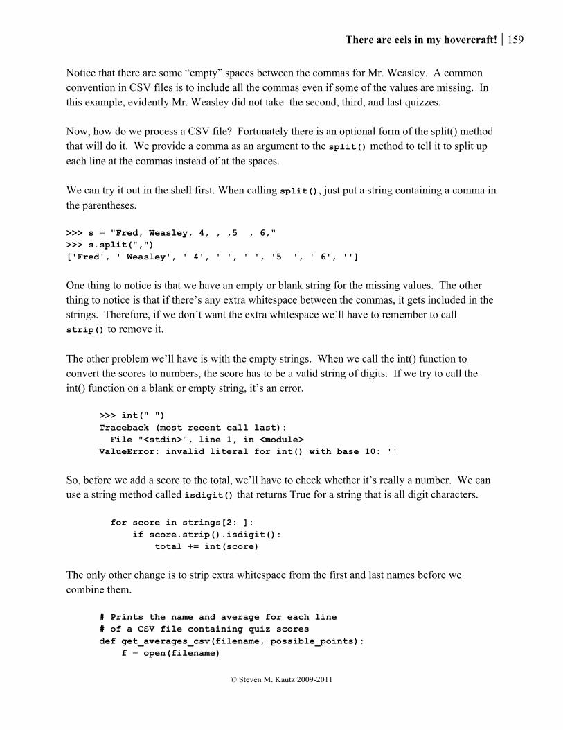
There are eels in my hovercraft! 159
© Steven M. Kautz 2009-2011
Notice that there are some “empty” spaces between the commas for Mr. Weasley. A common convention in CSV files is to include all the commas even if some of the values are missing. In this example, evidently Mr. Weasley did not take the second, third, and last quizzes. Now, how do we process a CSV file? Fortunately there is an optional form of the split() method that will do it. We provide a comma as an argument to the split() method to tell it to split up each line at the commas instead of at the spaces. We can try it out in the shell first. When calling split(), just put a string containing a comma in the parentheses. >>> s = "Fred, Weasley, 4, , ,5 , 6," >>> s.split(",") ['Fred', ' Weasley', ' 4', ' ', ' ', '5 ', ' 6', '']
One thing to notice is that we have an empty or blank string for the missing values. The other thing to notice is that if there’s any extra whitespace between the commas, it gets included in the strings. Therefore, if we don’t want the extra whitespace we’ll have to remember to call strip() to remove it. The other problem we’ll have is with the empty strings. When we call the int() function to convert the scores to numbers, the score has to be a valid string of digits. If we try to call the int() function on a blank or empty string, it’s an error.
>>> int(" ") Traceback (most recent call last): File "<stdin>", line 1, in <module> ValueError: invalid literal for int() with base 10: ''
So, before we add a score to the total, we’ll have to check whether it’s really a number. We can use a string method called isdigit() that returns True for a string that is all digit characters. for score in strings[2: ]: if score.strip().isdigit(): total += int(score)
The only other change is to strip extra whitespace from the first and last names before we combine them.
# Prints the name and average for each line # of a CSV file containing quiz scores def get_averages_csv(filename, possible_points): f = open(filename)

160 Reading text files
© Steven M. Kautz 2009-2011
for line in f: strings = line.split(",") name = strings[0].strip() + " " + strings[1].strip() total = 0.0 for score in strings[2: ]: if score.strip().isdigit(): total += int(score) average = 100 * total / possible_points print name, average f.close()
19.5. Reading a file with the readlines() function
The most common way to read a file is to process the lines one at a time using a for-loop, as we have been doing. But sometimes we need to treat some of the lines specially, or iterate over just part of the file. As an example, suppose the file containing quiz scores actually starts out with a “header” at the beginning, say, two lines describing the contents and giving the total possible points:
# Names and quiz scores for Fall term # Possible points: 60 Hermione Granger 10 10 10 10 10 10 Fred Weasley 4 5 6 Harry Potter 8 9 8 10 3 10
A good way to handle this is with the readlines() method, which returns all the lines of the file as a list of strings. Then we can directly examine the second line and extract the possible points. f = open(filename) all = f.readlines() second_line = all[1] i = second_line.find(":") possible_points = int(second_line[i + 1:])
Next, we want to iterate over the lines of the file as before, but only starting with the third line. We can do this by taking a “slice” of the list of all lines, starting at index 2: for line in all[2: ]: # as before
The complete function is shown below. Notice that in this example the number of possible points isn’t an argument to the function, since it is read from the file.
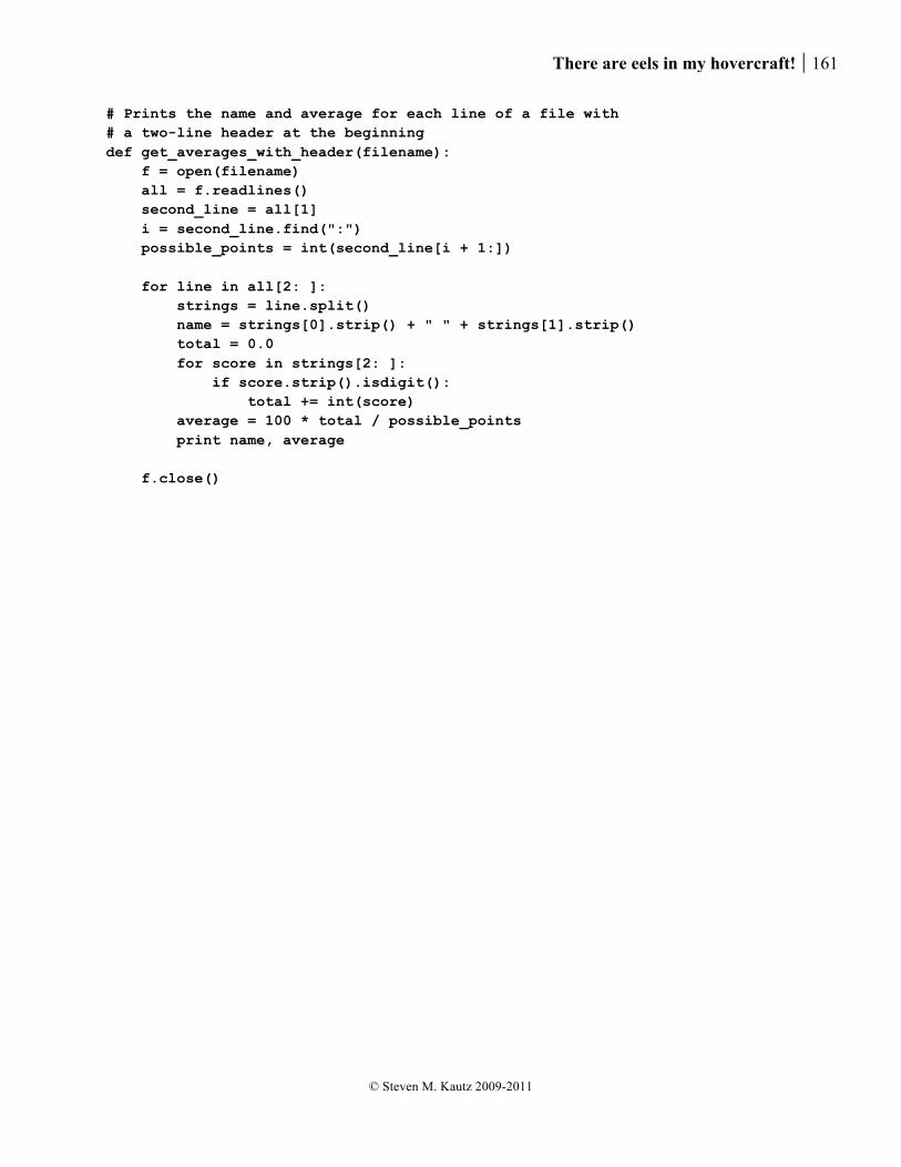
There are eels in my hovercraft! 161
© Steven M. Kautz 2009-2011
# Prints the name and average for each line of a file with # a two-line header at the beginning def get_averages_with_header(filename): f = open(filename) all = f.readlines() second_line = all[1] i = second_line.find(":") possible_points = int(second_line[i + 1:]) for line in all[2: ]: strings = line.split() name = strings[0].strip() + " " + strings[1].strip() total = 0.0 for score in strings[2: ]: if score.strip().isdigit(): total += int(score) average = 100 * total / possible_points print name, average f.close()

162 Writing text files
© Steven M. Kautz 2009-2011
20. Writing text files In this chapter we will learn how to create and write to text files.
20.1. Opening a file in write mode
There is an optional second argument to the open() function that you use when you want to create or write to a file. For text files, the three main possibilities are open(filename, ‘r’) open the file to read it (this is the default if no option is specified) open(filename, ‘w’) open the file to write to it as a new file open(filename, ‘a’) open the file to append, or add on, to its existing contents With the ‘r’ option, if the file doesn’t exist, you get an error. But with ‘a’ or ‘w’, if the named file doesn’t exist, a new, empty file is created. Be careful, though: when you open an existing file with the ‘w’ option, its contents are overwritten.
WARNING WARNING WARNING WARNING When you open a file with the ‘w’ option, if the file exists already, the contents of the existing file are immediately destroyed.
You can write text to a file using the method write(). Here is a short example. We’ll use the open() function with the “w” option to create a new file called “out.txt”.
myfile = open("out.txt", 'w') myfile.write("Hello ") myfile.write("world!") myfile.write("\n") myfile.write("Here is another line.") myfile.write("\n") myfile.close()
We can run this script and then examine the file “out.txt” using Notepad or another text editor. The file will be located in the same directory as the script. Here’s what the file looks like.

There are eels in my hovercraft! 163
© Steven M. Kautz 2009-2011
File: out.txt
Hello world! Here is another line.
Using the write() method is different than using the print keyword in two ways:
• The argument to write() must be a string. • The write() method does not automatically put a newline in the output. When we want
the output file to go to the next line, we have to explicitly write a newline character. It’s important to call the close() method when you’re finished writing to a file. Normally, writing to a file only updates a temporary buffer in the computer’s memory. Calling the close() method causes the operating system to actually update the hard drive, or other device, with the contents of the buffer. The file really isn’t permanently saved until the close() method is called. Here is another simple example. We know how to write a loop that reads numbers entered by the user, and computes their sum or average. A more practical approach would be to write the numbers into a file that can be saved and processed later. We can start with the same loop as before, where the user can enter the letter “q” to stop, and write each number to an output file. We would like each value on a separate line, so we’ll write a newline character after each value. The name of the output file is a parameter to the function. # Creates a simple output file containing # numbers entered at the console def create_number_file(filename): num_file = open(filename, 'w') response = raw_input("Enter a number (q to quit): ") while (response != "q"): num_file.write(response) num_file.write("\n") response = raw_input("Enter a number (q to quit): ") num_file.close()
20.2. Errors
When you want to read a file, the only thing that can go wrong is that the file isn’t there. When it comes to writing a file, there are different potential problems. Most operating systems have some kind of mechanism for access restrictions to directories or files. On Windows, a file or
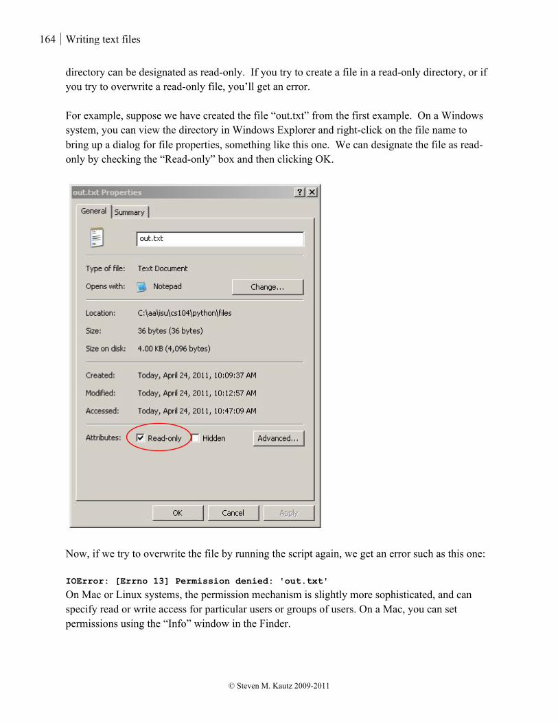
164 Writing text files
© Steven M. Kautz 2009-2011
directory can be designated as read-only. If you try to create a file in a read-only directory, or if you try to overwrite a read-only file, you’ll get an error. For example, suppose we have created the file “out.txt” from the first example. On a Windows system, you can view the directory in Windows Explorer and right-click on the file name to bring up a dialog for file properties, something like this one. We can designate the file as read-only by checking the “Read-only” box and then clicking OK.
Now, if we try to overwrite the file by running the script again, we get an error such as this one: IOError: [Errno 13] Permission denied: 'out.txt'
On Mac or Linux systems, the permission mechanism is slightly more sophisticated, and can specify read or write access for particular users or groups of users. On a Mac, you can set permissions using the “Info” window in the Finder.
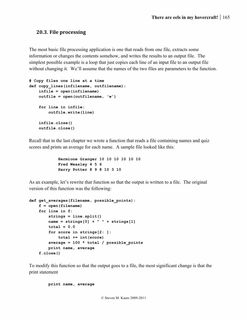
There are eels in my hovercraft! 165
© Steven M. Kautz 2009-2011
20.3. File processing
The most basic file processing application is one that reads from one file, extracts some information or changes the contents somehow, and writes the results to an output file. The simplest possible example is a loop that just copies each line of an input file to an output file without changing it. We’ll assume that the names of the two files are parameters to the function. # Copy files one line at a time def copy_lines(infilename, outfilename): infile = open(infilename) outfile = open(outfilename, 'w') for line in infile: outfile.write(line) infile.close() outfile.close()
Recall that in the last chapter we wrote a function that reads a file containing names and quiz scores and prints an average for each name. A sample file looked like this:
Hermione Granger 10 10 10 10 10 10 Fred Weasley 4 5 6 Harry Potter 8 9 8 10 3 10
As an example, let’s rewrite that function so that the output is written to a file. The original version of this function was the following: def get_averages(filename, possible_points): f = open(filename) for line in f: strings = line.split() name = strings[0] + " " + strings[1] total = 0.0 for score in strings[2: ]: total += int(score) average = 100 * total / possible_points print name, average f.close()
To modify this function so that the output goes to a file, the most significant change is that the print statement print name, average
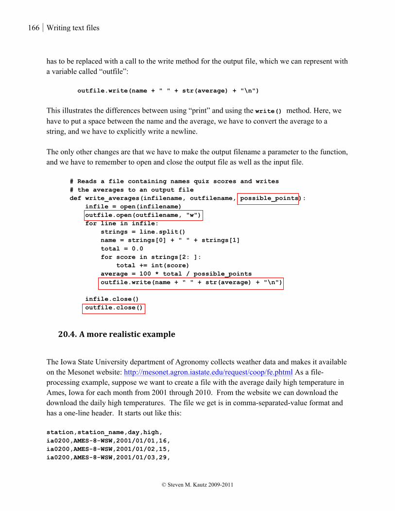
166 Writing text files
© Steven M. Kautz 2009-2011
has to be replaced with a call to the write method for the output file, which we can represent with a variable called “outfile”: outfile.write(name + " " + str(average) + "\n")
This illustrates the differences between using “print” and using the write() method. Here, we have to put a space between the name and the average, we have to convert the average to a string, and we have to explicitly write a newline. The only other changes are that we have to make the output filename a parameter to the function, and we have to remember to open and close the output file as well as the input file.
# Reads a file containing names quiz scores and writes # the averages to an output file def write_averages(infilename, outfilename, possible_points): infile = open(infilename) outfile.open(outfilename, "w") for line in infile: strings = line.split() name = strings[0] + " " + strings[1] total = 0.0 for score in strings[2: ]: total += int(score) average = 100 * total / possible_points outfile.write(name + " " + str(average) + "\n") infile.close() outfile.close()
20.4. A more realistic example
The Iowa State University department of Agronomy collects weather data and makes it available on the Mesonet website: http://mesonet.agron.iastate.edu/request/coop/fe.phtml As a file-processing example, suppose we want to create a file with the average daily high temperature in Ames, Iowa for each month from 2001 through 2010. From the website we can download the download the daily high temperatures. The file we get is in comma-separated-value format and has a one-line header. It starts out like this: station,station_name,day,high, ia0200,AMES-8-WSW,2001/01/01,16, ia0200,AMES-8-WSW,2001/01/02,15, ia0200,AMES-8-WSW,2001/01/03,29,

There are eels in my hovercraft! 167
© Steven M. Kautz 2009-2011
ia0200,AMES-8-WSW,2001/01/04,36, ia0200,AMES-8-WSW,2001/01/05,40, ia0200,AMES-8-WSW,2001/01/06,40, ia0200,AMES-8-WSW,2001/01/07,36, ia0200,AMES-8-WSW,2001/01/08,26, ...
There is one line for each day in the ten-year period we have selected. But remember, what we really want are the average high temperatures for each month. That is, we would like an output file in which each line has the form “month/year” followed by the average high temperature for that month, like this: 01/2001 30.1 02/2001 26.5 03/2001 38.1 04/2001 67.6 05/2001 71.6 ...
We can read the input file one line at a time and add the temperatures to a total. But when we get to the end of the month, then we need to compute the average temperature, and write one line to the output file. How will we be able to tell when we’ve gotten to the end of the month? Well, probably the easiest way to do it is to keep track of the “current” month, and as soon as we read a line for a different month, then we’ll know it’s time to write a line of output and start over for the next month. In order to compute the average, we’ll also need to count the temperatures as we add them to the total. We can try to summarize our reasoning in pseudocode like this:
for each line of the input file if the line is for a different month than the current month find the average write the month, year, and average to the output file reset the total to zero reset the count to zero add the temperature to the total add 1 to the count
This is not an easy problem, so we’ll try to work on it “incrementally” instead of all at once. Notice first that there are some simple sub-problems we can tackle independently. For example, given one line of the file, we’ll need to extract the month, the year, and the temperature. We can

168 Writing text files
© Steven M. Kautz 2009-2011
experiment a bit in the shell using a sample line of the file. Recall first that we can use the string split() method to split the string at the commas. >>> test = "ia0200,AMES-8-WSW,2008/01/01,16," >>> strings = test.split(",") >>> strings ['ia0200', 'AMES-8-WSW', '2008/01/01', '16', '']
So the date is the string at index 2: >>> date = strings[2] >>> date '2008/01/01'
The year will always be the first four characters of that string, and the month will be the substring at positions 5 through 6 >>> date[ :4] '2008' >>> date[5:7] '01'
Likewise, the temperature is always at index 3 of the list. >>> strings[3] '16'
We can isolate these tasks in a couple of “helper” functions in order to try to simplify the main loop. # Returns the year from one line of the file def get_year(s): strings = s.split(",") date = strings[2] return date[ :4] # Returns the month from one line of the file def get_month(s): strings = s.split(",") date = strings[2] return date[5:7] # Returns the temperature from one line of the file def get_temp(s): strings = s.split(",") return int(strings[3])
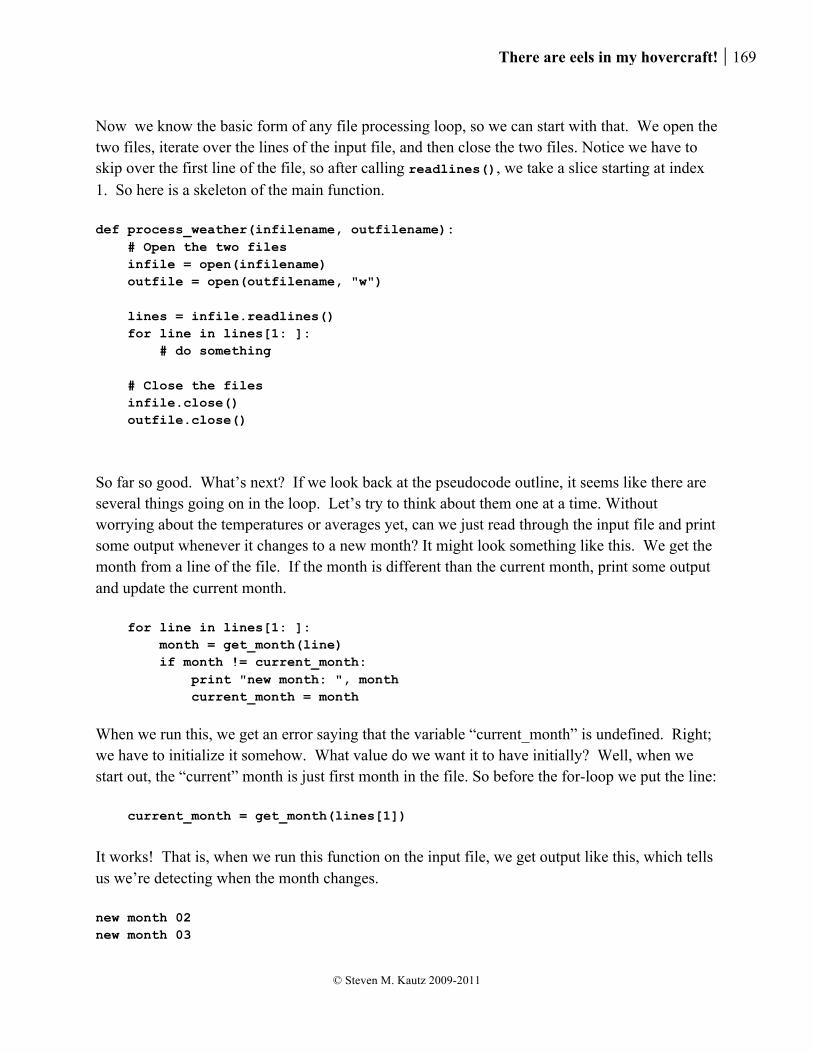
There are eels in my hovercraft! 169
© Steven M. Kautz 2009-2011
Now we know the basic form of any file processing loop, so we can start with that. We open the two files, iterate over the lines of the input file, and then close the two files. Notice we have to skip over the first line of the file, so after calling readlines(), we take a slice starting at index 1. So here is a skeleton of the main function. def process_weather(infilename, outfilename): # Open the two files infile = open(infilename) outfile = open(outfilename, "w") lines = infile.readlines() for line in lines[1: ]: # do something # Close the files infile.close() outfile.close()
So far so good. What’s next? If we look back at the pseudocode outline, it seems like there are several things going on in the loop. Let’s try to think about them one at a time. Without worrying about the temperatures or averages yet, can we just read through the input file and print some output whenever it changes to a new month? It might look something like this. We get the month from a line of the file. If the month is different than the current month, print some output and update the current month. for line in lines[1: ]: month = get_month(line) if month != current_month: print "new month: ", month current_month = month
When we run this, we get an error saying that the variable “current_month” is undefined. Right; we have to initialize it somehow. What value do we want it to have initially? Well, when we start out, the “current” month is just first month in the file. So before the for-loop we put the line: current_month = get_month(lines[1])
It works! That is, when we run this function on the input file, we get output like this, which tells us we’re detecting when the month changes. new month 02 new month 03

170 Writing text files
© Steven M. Kautz 2009-2011
new month 04 new month 05 ...
Now, let’s add statements to add up the temperatures and count them so we can compute an average. As usual, we’ll start out a total and a counter at zero: total = 0.0 count = 0
and each time we go through the loop, we add the temperature to the total, and add 1 to the counter. We’ll initialize a current year too, since we’ll eventually have to print that as well. current_month = get_month(lines[1]) current_year = get_year(lines[1]) total = 0.0 count = 0 lines = infile.readlines() for line in lines[1: ]: month = get_month(line) if month != current_month: print "new month: ", month current_month = month temp = get_temp(line) total += temp count += 1
The part that’s missing now is to actually compute the average when we get to the end of the month, and write it to the file. So we replace the print statement with a call to the write() method. But each time we do this, we have to restart the total and counter at zero. if month != current_month: average = total / count outfile.write(current_month + "/" + current_year + " ") outfile.write(str(average) + "\n") current_month = month total = 0.0 count = 0 current_year = get_year(line) temp = get_temp(line) total += temp count += 1
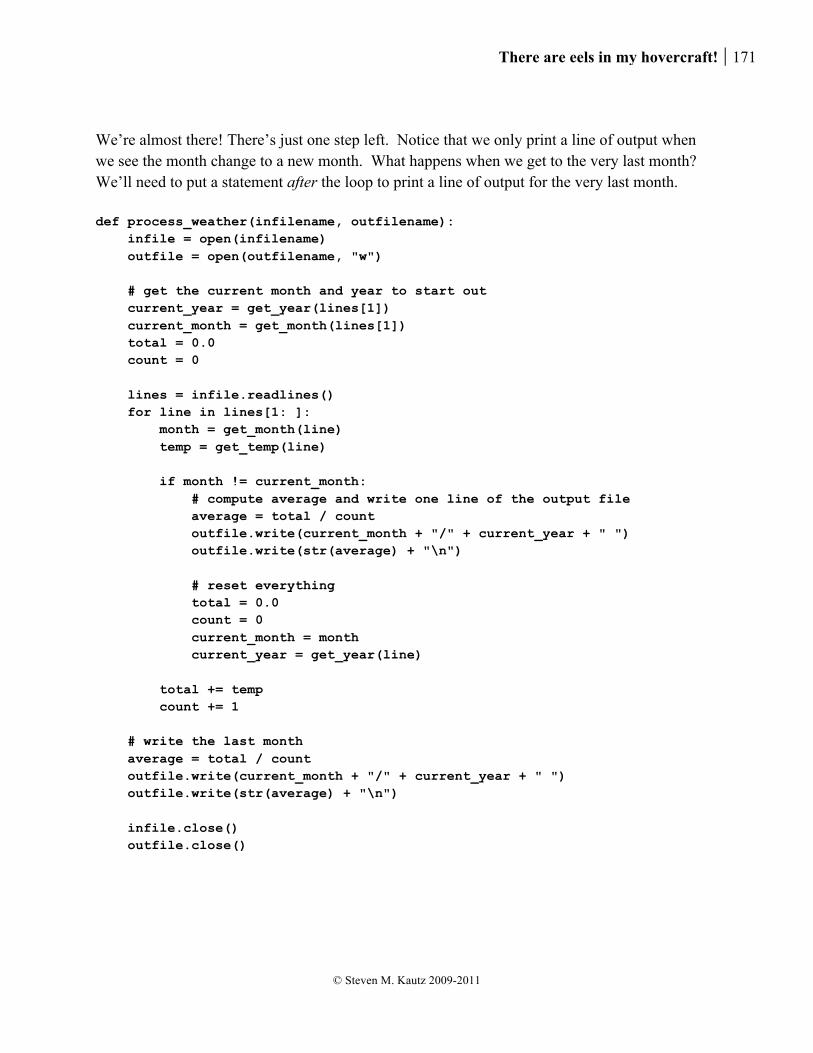
There are eels in my hovercraft! 171
© Steven M. Kautz 2009-2011
We’re almost there! There’s just one step left. Notice that we only print a line of output when we see the month change to a new month. What happens when we get to the very last month? We’ll need to put a statement after the loop to print a line of output for the very last month. def process_weather(infilename, outfilename): infile = open(infilename) outfile = open(outfilename, "w") # get the current month and year to start out current_year = get_year(lines[1]) current_month = get_month(lines[1]) total = 0.0 count = 0 lines = infile.readlines() for line in lines[1: ]: month = get_month(line) temp = get_temp(line) if month != current_month: # compute average and write one line of the output file average = total / count outfile.write(current_month + "/" + current_year + " ") outfile.write(str(average) + "\n") # reset everything total = 0.0 count = 0 current_month = month current_year = get_year(line) total += temp count += 1 # write the last month average = total / count outfile.write(current_month + "/" + current_year + " ") outfile.write(str(average) + "\n") infile.close() outfile.close()
172 File paths and command shells
© Steven M. Kautz 2009-2011
21. File paths and command shells In the last two chapters we have learned the basics of file-processing in Python. You’ll find these techniques are extremely useful, but to make the most of them we’ll have to understand some more about the file system of a typical computer. We’ll do this by learning a little bit about how to use a command shell. We’ll also learn how to run Python scripts without having to start up a programming environment such as IDLE or DrPython. Most of the applications you use on a computer these days have a graphical user interface. The application runs in one or more windows on the screen, and there are controls such as menus and buttons that you can manipulate with a mouse. But many very useful applications don't have a graphical interface. Instead, you run them from a command shell. A command shell is a text-based interface. It displays a prompt and waits for you to type a command, kind of like the Python shell. But while the Python shell lets you interact with the Python interpreter, a command shell lets you interact directly with your computer's operating system and files. For many kinds of tasks, using a command shell is a much more efficient way to do things than dragging icons around with a mouse. The exact details of how a command shell works depend on the operating system you are using, so for the first time in this course, it will make a difference whether you’re using a Windows system or a Mac. We'll give most of the examples using the Windows conventions, and try to note the differences for Mac users. If you use Linux, most of the remarks for Macs will apply to your system too. The first thing we need to do is figure out how to "navigate" through the file system. For that, let's briefly review how files and directories are organized.
21.1. The path to a file
Every file is stored on some kind of device. A device may be a real piece of hardware you can get your hands on, like the hard drive on your computer or a flash drive you can plug into a USB port. A device could also be “virtual”, for example, you might store files on a network server that is, in reality, shared by many users. A device allows you to organize your files into directories. Remember that directories are also called “folders”. Every file is in some directory, which could be inside of some other directory, which could be inside of some other directory, and so on. But it can’t go on forever. Eventually, you get to a directory at the top that isn’t inside of any other directory, which is called the “root directory” for the device.

There are eels in my hovercraft! 173
© Steven M. Kautz 2009-2011
cs104
username
chapter21 chapter19
testfile.txt_______________
temp
(root)
Users
Figure 1 - Absolute path to testfile.txt
Every file or directory has a name. But the name alone isn’t enough to find it. For example, you might have several files with the same name in different places. A file can be identified uniquely by an “absolute path”. That is the sequence of directories you would have to follow to find it, starting at the root directory of whatever device it’s stored on. For example, many computers are organized so that in the root directory of the hard drive there is a directory, often called “Users”, that has subdirectories for each user, identified by usernames. This is sometimes called your “home” directory for a user, and many applications will store your files somewhere in your home directory. Then in your home directory, suppose there is a directory “cs104” which has a sub-directory “chapter21”, and inside that directory you have a file called “testfile.txt”. Then the absolute path to the file can be described by saying Start at the root of the device Go into the Users directory Then go into my home directory

174 File paths and command shells
© Steven M. Kautz 2009-2011
Then go into the cs104 directory Then go into the chapter21 directory Then find the file named “testfile.txt” Each operating system has its own notation for paths. On Windows, devices are identified by letters, and the hard drive of a personal.computer is usually labeled “C colon backslash”. The path is usually written with backward slashes to separate the directories in the path, so the path to our file testfile.txt would be written: C:\Users\username\cs104\chapter21\testfile.txt
On a Mac, the root of the device is just a forward slash, and you use forward slashes between the directories, so the same path would be written /Users/username/cs104/chapter21/testfile.txt
21.2. The working directory and some basic commands
To start a command shell on Windows, go to “All Programs” in the Start menu, select “Accessories”, and then “Command Prompt” It usually looks something like this:
To start a command shell on a Mac, open a Finder. Under "Places", select "Applications". Then double-click on the "Utilities" folder and find the icon for "Terminal" and double-click it.

There are eels in my hovercraft! 175
© Steven M. Kautz 2009-2011
The command shell on a Mac looks something like this:
The first thing to notice is that the command shell always has a “current directory” or “working directory”. This is normally shown as part of the prompt. The Windows prompt is usually some text followed by the “greater-than” character (“>”).
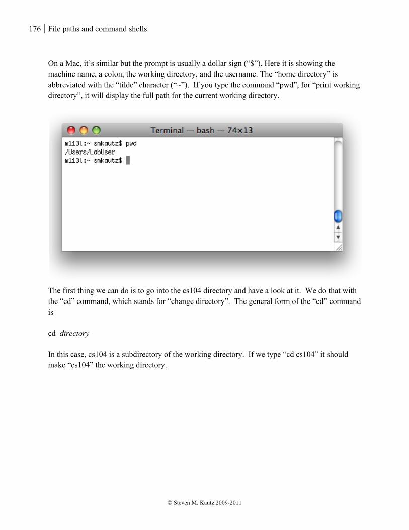
176 File paths and command shells
© Steven M. Kautz 2009-2011
On a Mac, it’s similar but the prompt is usually a dollar sign (“$”). Here it is showing the machine name, a colon, the working directory, and the username. The “home directory” is abbreviated with the “tilde” character (“~”). If you type the command “pwd”, for “print working directory”, it will display the full path for the current working directory.
The first thing we can do is to go into the cs104 directory and have a look at it. We do that with the “cd” command, which stands for “change directory”. The general form of the “cd” command is cd directory In this case, cs104 is a subdirectory of the working directory. If we type “cd cs104” it should make “cs104” the working directory.

There are eels in my hovercraft! 177
© Steven M. Kautz 2009-2011
It works the same way on a Mac. Notice that on a Mac, the commands are case-sensitive, while on Windows, they’re not. The next thing you might want to do is to look at what files are in the working directory. On Windows, you use the command “dir”. Here we can see the two subdirectories chapter21 and chapter 19, which are labeled “DIR”. On the left of each line is the date and time when it was last modified.
The corresponding command for a Mac is “ls” which is some perverse kind of abbreviation for “list”.

178 File paths and command shells
© Steven M. Kautz 2009-2011
By default, the listing only shows the names. To get more detail, type ls –l (“ls space dash l”).
Each line starts with a string of characters, most of which we can ignore for the time being. However, if the first character is “d”, that means it is a directory. Next we can go into the “chapter21” directory by typing “cd chapter21”. Again typing “dir” for a directory listing, we can see the file testfile.txt. The number to the left of the name is the size of the file in bytes.
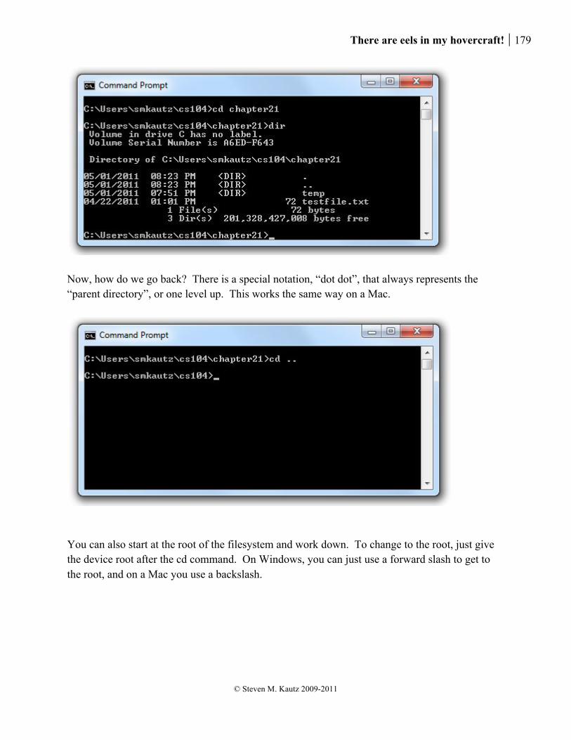
There are eels in my hovercraft! 179
© Steven M. Kautz 2009-2011
Now, how do we go back? There is a special notation, “dot dot”, that always represents the “parent directory”, or one level up. This works the same way on a Mac.
You can also start at the root of the filesystem and work down. To change to the root, just give the device root after the cd command. On Windows, you can just use a forward slash to get to the root, and on a Mac you use a backslash.

180 File paths and command shells
© Steven M. Kautz 2009-2011
There is also a command for printing the contents of a text file. On Windows it is called “type”. Let’s return to the chapter21 directory to try it.
On a Mac, the “cat” command is used.
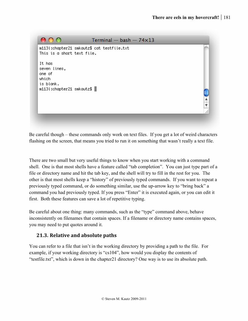
There are eels in my hovercraft! 181
© Steven M. Kautz 2009-2011
Be careful though – these commands only work on text files. If you get a lot of weird characters flashing on the screen, that means you tried to run it on something that wasn’t really a text file. There are two small but very useful things to know when you start working with a command shell. One is that most shells have a feature called “tab completion”. You can just type part of a file or directory name and hit the tab key, and the shell will try to fill in the rest for you. The other is that most shells keep a “history” of previously typed commands. If you want to repeat a previously typed command, or do something similar, use the up-arrow key to “bring back” a command you had previously typed. If you press “Enter” it is executed again, or you can edit it first. Both these features can save a lot of repetitive typing. Be careful about one thing: many commands, such as the “type” command above, behave inconsistently on filenames that contain spaces. If a filename or directory name contains spaces, you may need to put quotes around it.
21.3. Relative and absolute paths
You can refer to a file that isn’t in the working directory by providing a path to the file. For example, if your working directory is “cs104”, how would you display the contents of “testfile.txt”, which is down in the chapter21 directory? One way is to use its absolute path.

182 File paths and command shells
© Steven M. Kautz 2009-2011
Remember that on a Mac, the absolute path starts with a forward slash.
But you can also use a “relative” path, which describes how to find the file from the working directory, rather than from the root. From cs104, you can describe how to get to testfile.txt by saying First go into the chapter21 directory Then find testfile.txt
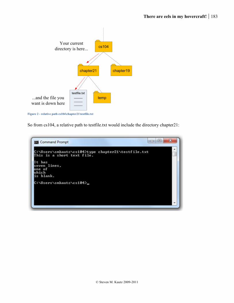
There are eels in my hovercraft! 183
© Steven M. Kautz 2009-2011
cs104
chapter21 chapter19
testfile.txt_______________
Your current directory is here...
...and the file you want is down here
temp
Figure 2 - relative path cs104\chapter21\testfile.txt
So from cs104, a relative path to testfile.txt would include the directory chapter21:
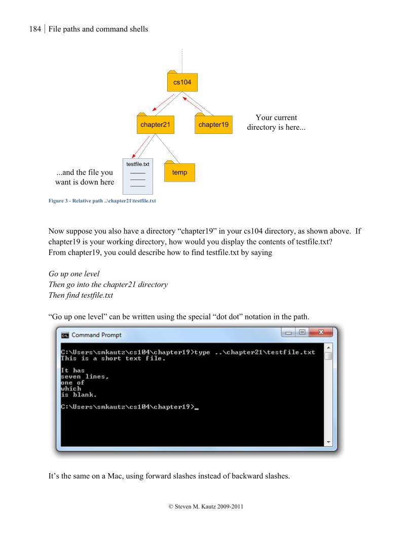
184 File paths and command shells
© Steven M. Kautz 2009-2011
cs104
chapter21 chapter19
testfile.txt_______________
Your current directory is here...
...and the file you want is down here
temp
Figure 3 - Relative path ..\chapter21\testfile.txt
Now suppose you also have a directory “chapter19” in your cs104 directory, as shown above. If chapter19 is your working directory, how would you display the contents of testfile.txt? From chapter19, you could describe how to find testfile.txt by saying Go up one level Then go into the chapter21 directory Then find testfile.txt “Go up one level” can be written using the special “dot dot” notation in the path.
It’s the same on a Mac, using forward slashes instead of backward slashes.
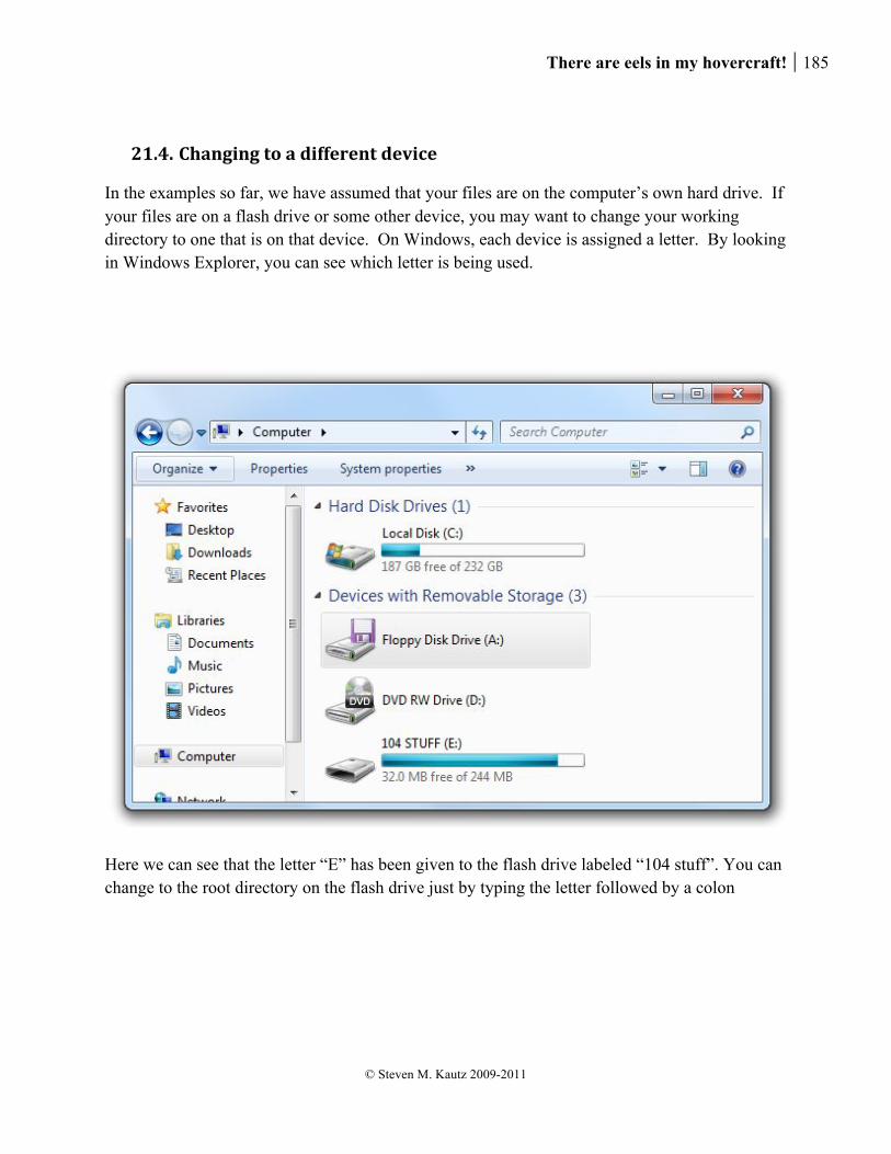
There are eels in my hovercraft! 185
© Steven M. Kautz 2009-2011
21.4. Changing to a different device
In the examples so far, we have assumed that your files are on the computer’s own hard drive. If your files are on a flash drive or some other device, you may want to change your working directory to one that is on that device. On Windows, each device is assigned a letter. By looking in Windows Explorer, you can see which letter is being used.
Here we can see that the letter “E” has been given to the flash drive labeled “104 stuff”. You can change to the root directory on the flash drive just by typing the letter followed by a colon
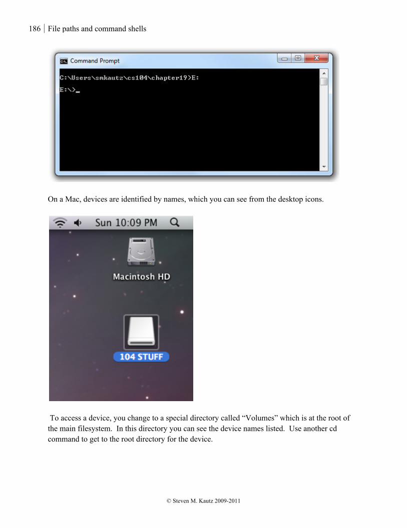
186 File paths and command shells
© Steven M. Kautz 2009-2011
On a Mac, devices are identified by names, which you can see from the desktop icons.
To access a device, you change to a special directory called “Volumes” which is at the root of the main filesystem. In this directory you can see the device names listed. Use another cd command to get to the root directory for the device.

There are eels in my hovercraft! 187
© Steven M. Kautz 2009-2011
21.5. Running a Python script
Up until now, you have run your programs from a development environment such as IDLE or DrPython. This is convenient when you’re writing and testing the code, but once it is done and you no longer need to edit the code, there is no reason to have to start up the development environment just to run the program. You can do it from a command shell by directly invoking the Python interpreter. The interpreter itself is an executable file. That means that it has been translated into direct instructions for your computer’s processor. By contrast, the Python scripts we write aren’t executable. They have to be read and run by the Python interpreter. Normally you can run an executable from the command shell by typing the name of the file. For example, the simple Notepad text editor is an executable called “notepad.exe”. You can start it from your command shell by typing “notepad” at the command prompt.

188 File paths and command shells
© Steven M. Kautz 2009-2011
The Python interpreter on Windows is an executable called “python.exe”. However, if you have the default Python installation, you won’t be able to just type “python” in a command shell.
The command shell doesn’t know where to find “python.exe”. In this case, you just have to provide a path to the file. The executable for the Python interpreter is normally located in C:\Python26. The name may be slightly different depending on the version you have. We can take a look using Windows Explorer.
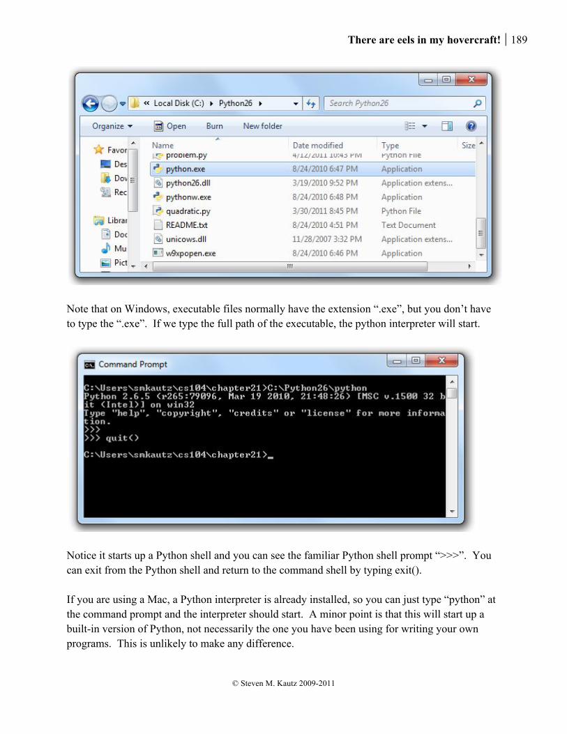
There are eels in my hovercraft! 189
© Steven M. Kautz 2009-2011
Note that on Windows, executable files normally have the extension “.exe”, but you don’t have to type the “.exe”. If we type the full path of the executable, the python interpreter will start.
Notice it starts up a Python shell and you can see the familiar Python shell prompt “>>>”. You can exit from the Python shell and return to the command shell by typing exit(). If you are using a Mac, a Python interpreter is already installed, so you can just type “python” at the command prompt and the interpreter should start. A minor point is that this will start up a built-in version of Python, not necessarily the one you have been using for writing your own programs. This is unlikely to make any difference.
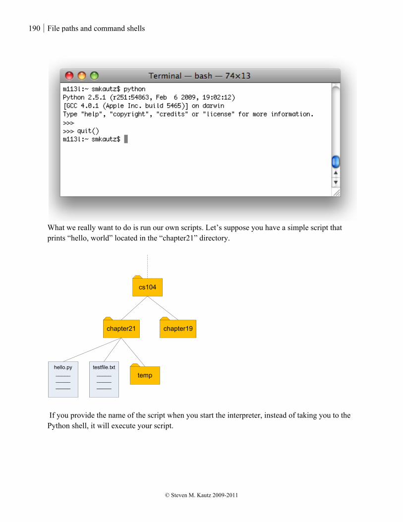
190 File paths and command shells
© Steven M. Kautz 2009-2011
What we really want to do is run our own scripts. Let’s suppose you have a simple script that prints “hello, world” located in the “chapter21” directory.
cs104
chapter21 chapter19
testfile.txt_______________
temphello.py_______________
If you provide the name of the script when you start the interpreter, instead of taking you to the Python shell, it will execute your script.
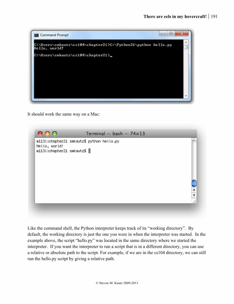
There are eels in my hovercraft! 191
© Steven M. Kautz 2009-2011
It should work the same way on a Mac:
Like the command shell, the Python interpreter keeps track of its “working directory”. By default, the working directory is just the one you were in when the interpreter was started. In the example above, the script “hello.py” was located in the same directory where we started the interpreter. If you want the interpreter to run a script that is in a different directory, you can use a relative or absolute path to the script. For example, if we are in the cs104 directory, we can still run the hello.py script by giving a relative path.
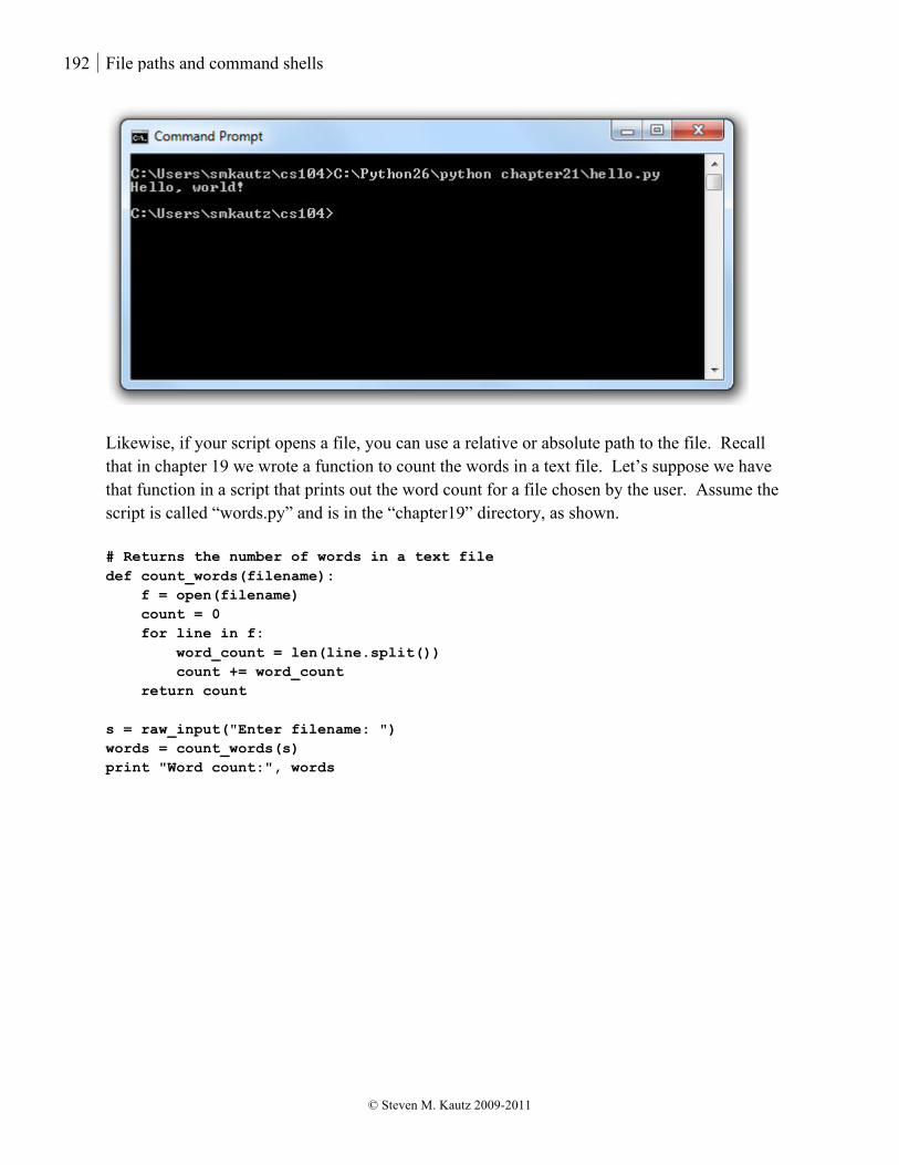
192 File paths and command shells
© Steven M. Kautz 2009-2011
Likewise, if your script opens a file, you can use a relative or absolute path to the file. Recall that in chapter 19 we wrote a function to count the words in a text file. Let’s suppose we have that function in a script that prints out the word count for a file chosen by the user. Assume the script is called “words.py” and is in the “chapter19” directory, as shown. # Returns the number of words in a text file def count_words(filename): f = open(filename) count = 0 for line in f: word_count = len(line.split()) count += word_count return count s = raw_input("Enter filename: ") words = count_words(s) print "Word count:", words
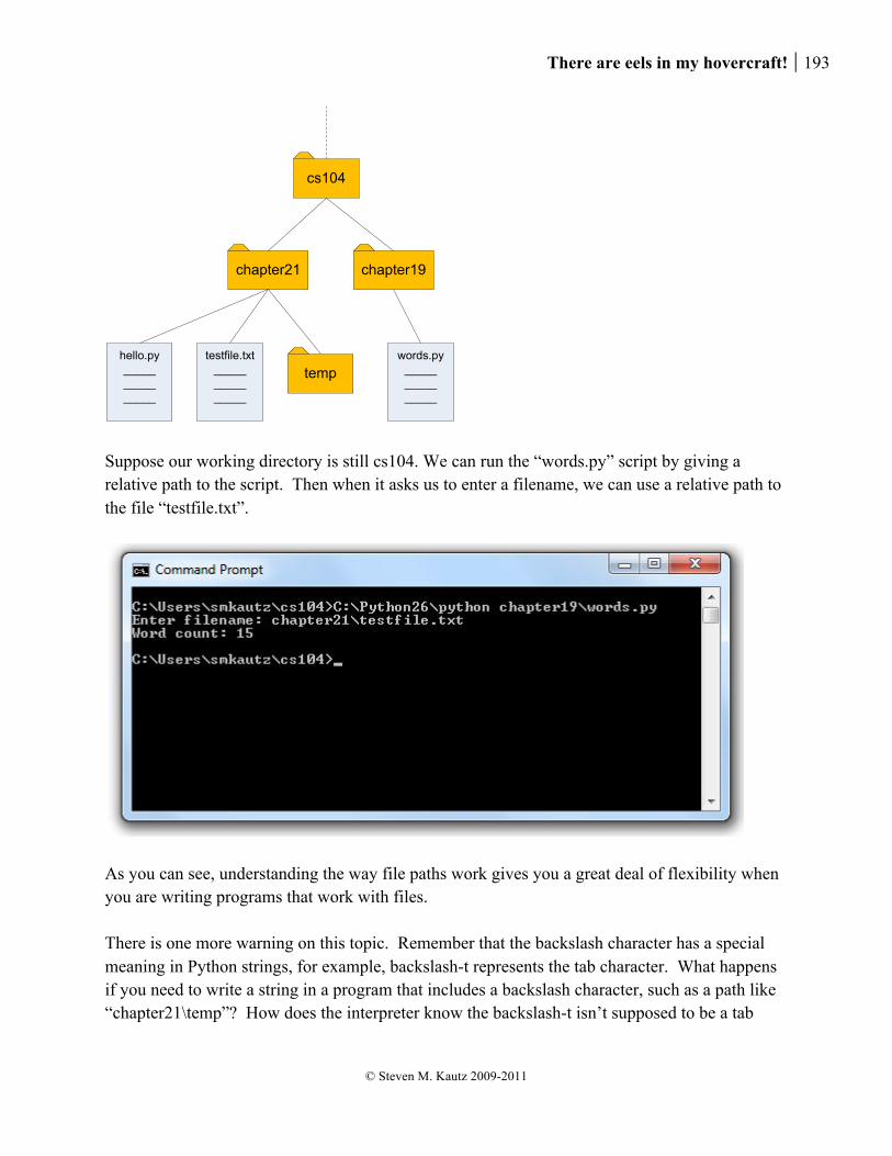
There are eels in my hovercraft! 193
© Steven M. Kautz 2009-2011
cs104
chapter21 chapter19
testfile.txt_______________
temphello.py_______________
words.py_______________
Suppose our working directory is still cs104. We can run the “words.py” script by giving a relative path to the script. Then when it asks us to enter a filename, we can use a relative path to the file “testfile.txt”.
As you can see, understanding the way file paths work gives you a great deal of flexibility when you are writing programs that work with files. There is one more warning on this topic. Remember that the backslash character has a special meaning in Python strings, for example, backslash-t represents the tab character. What happens if you need to write a string in a program that includes a backslash character, such as a path like “chapter21\temp”? How does the interpreter know the backslash-t isn’t supposed to be a tab

194 File paths and command shells
© Steven M. Kautz 2009-2011
character? What you have to do is write “backslash backslash” whenever you really want a backslash in the string.
21.6. Command-‐line arguments
In the word-counting script, we had to use an input statement to read the filename. It is also possible to provide the filename directly to the interpreter along with the name of the script. This is done with command-line arguments. The idea is simple. When you invoke the interpreter, you always provide the name of the script. But anything extra you type on the command line is available for you to use inside the script. The extra stuff is stored in a list of strings called “argv”, which is part of a module called “sys”. Here is a simple script we’ll call “echo.py” that just prints out all the command-line arguments. import sys print sys.argv
If we invoke the echo.py script and follow the name by “foo bar baz”, the list looks like this.
Notice that argv[0] is always the name of the script itself. So the next piece of text after that is argv[1], and so on. We can change our words.py script from an interactive program into a command-line program.

There are eels in my hovercraft! 195
© Steven M. Kautz 2009-2011
import sys # Returns the number of words in a text file def count_words(filename): f = open(filename) count = 0 for line in f: word_count = len(line.split()) count += word_count return count if len(sys.argv) >= 2: s = sys.argv[1] else: s = raw_input("Enter filename: ") words = count_words(s) print "Word count:", words
If the user supplies a filename on the command line, we’ll be able to check that the length of “argv” is at least 2. If it is, we can use argv[1] for the filename, and the script doesn’t have to stop and wait for input.
21.7. Where to go next
We have introduced command shells as a way to talk in detail about file paths, and in order to show that you can run Python scripts directly, without the need for a programming environment like IDLE or DrPython. We have only looked at a couple of commands, and in reality we have hardly scratched the surface. There are many online resources that describe other shell
196 File paths and command shells
© Steven M. Kautz 2009-2011
commands and how to use them. Just remember to be careful when it comes to commands that modify system settings or that delete files.