Embed Size (px)
Citation preview


“There is nothing more practical than a good theory.”
James C. Maxwell
“. . . le souci du beau nous conduit aux memes choix que celui de l’utile.”
Henri Poincare

Preface
Many phenomena in science and technology are dynamical in nature. Sta-
tionary regimes, periodic motions and beats from modulations have long been
believed to be the only possible observable states. However, discoveries in the
second half of the 20th century have dramatically changed our traditional view
of the character of dynamical processes. The breakthrough came with the dis-
covery of a new type of oscillations called dynamical chaos. A deepening of our
understanding of dynamical phenomena has since led us to a clear recognition
that ours is a nonlinear world. This has resulted in the emergence of nonlin-
ear dynamics as a scientific discipline whose aim is to study the common laws
(regularities) of nonlinear dynamical processes.
A typical scheme for investigating a new phenomenon usually proceeds as
follow: the relevant experiment or observation is studied by first construct-
ing an adequate mathematical model in the form of dynamical equations.
This model is analyzed and the result is compared with the experimental
phenomenon.
This approach was first suggested by Newton. The laws that Newton dis-
covered have provided a foundation for the mathematical modeling of numerous
problems, including Celestial mechanics. The solution of the restricted two-
body problem gives a brilliant explanation of the experimental Kepler’s laws.
In fact, starting with Newton, this method for modeling nature has dominated
the field for many years. However, even such a purely scientific approach
must be validated by questioning the correspondence between a real phe-
nomenon and its phenomenological model, which had been aptly put by Bril-
louin: “A mathematical model differs from reality just as a globe differs from
the earth”.
ix

x Preface
A mathematical model in nonlinear dynamics usually consists of a sys-
tem of equations with analytically given nonlinearities, and a finite number
of parameters. The system may be described by ordinary differential equa-
tions, partial differential equations, equations with a delay, integro-differential
equations, etc. In this book we will deal only with lumped (discrete-space)
systems described by ordinary differential equations. Furthermore, we will re-
strict ourselves to a study of non-conservative systems thereby leaving aside the
“ideal” dynamics of Hamiltonian systems (which Klein, at the end of the 19th
century, had characterized as being the most “attractive mechanics without
friction”).
A system of differential equations is written in the form
dx
dt= X(x) ,
where the independent variable t is called the time. One of the postulates of
nonlinear dynamics which dates back to Aristotle and is based on common
sense is that all observable states must be stable. This implies that in any
comprehensive study of systems of differential equations, our attention must
be focused on the character of the solutions over an infinite time interval. The
systems considered from this point of view are called dynamical. Although
the notion of a dynamical system is a mathematical abstraction — indeed
we know from cosmology that even our Universe has only a finite life time
— nevertheless, many phenomena of the real world have been successfully
explained via the theory of dynamical systems. In the language of this theory
the mathematical image of a stationary state is an equilibrium state, that of
self-oscillations is a limit cycle, that of modulation is an invariant torus with
a quasi-periodic trajectory, and the image of dynamical chaos is a strange
attractor; namely, an attracting limit set composed of unstable trajectories.
In principle, the first three types of motions cited may be explained by a
linear theory. That was the approach of the 19th century, which concerned
mainly various practical applications modeled in terms of linear ordinary or
partial differential equations. The most famous example is the problem of
controlling steam engines whose investigation had led to the solution of the
problem of stability of equilibrium states; namely to the classic Routh–Hurwitz
criterion.
The most remarkable events in nonlinear dynamics can be traced to the
twenties and the thirties of the 20th century. This period is characterized
by the rapid development of radio-engineering. A common feature of many

Preface xi
nonlinear radio-engineering problems is that the associated transient processes
are typically very fast, thereby making it less time-consuming to carry out
complicated experiments. The fact that the associated mathematical models
in those days are usually simple systems of quasi-linear equations also plays an
important role. This has in turn allowed researchers to conduct rather complete
investigations of the models using methods based on Poincare’s theory of limit
cycles and Lyapunov’s stability theory.
Another significant event from that period is the creation of a mathemati-
cal theory of oscillations in two-dimensional systems. In particular, Andronov
and Pontryagin identified a large class of rough (structurally stable) systems
which admit a rather simple mathematical description. Moreover, all prin-
cipal bifurcations of limit cycles were studied (Andronov, Leontovich) and
complete topological invariants for both rough systems (Andronov, Pontrya-
gin) and generic systems (Leontovich, Mayer) were described. Shortly after
that, specialists from various areas of research applied these mathematically
transparent and geometrically comprehensive methods to investigate concrete
two-dimensional systems. This stage of the development is documented in the
classic treatise “Theory of oscillations” by Andronov, Vitt and Khaikin.1
Further development in this subject included the attempt at a straight-
forward generalization of the concepts of planar systems, namely, the aim of
extending the conditions of structural stability and bifurcations to the high-
dimensional case. In no way does this approach indicate narrow visions. On
the contrary, this was a mathematically sound strategy. Indeed, it was un-
derstood that entrance into space must bring new types of motions which
may become crucial in nonlinear dynamics. As was mentioned previously, the
mathematical image of modulation is a torus with quasi-periodic trajectories.
Quasi-periodic trajectories are a particular case of almost-periodic trajectories
which, by definition, are unclosed trajectories whose main feature is that they
have almost-periods — the time intervals over which the trajectory returns
close to its initial state. The quasi- and almost-periodic trajectories are self-
limiting. A broader class of self-limiting trajectories consists of Poisson-stable
trajectories. This kind of trajectory was discovered by Poincare while studying
the stability of the restricted three-body problem. A Poisson-stable trajectory
also returns arbitrarily close to its initial state, but for an arbitrary but fixed
small neighborhood of the initial state, the sequence of the associated return
1This book was first published in 1937 but without the name of Vitt, who had alreadybeen repressed.

xii Preface
times may be unbounded, i.e. the motion is unpredictable. In accordance with
Birkhoff’s classification, stationary, periodic, quasi-periodic, almost-periodic
and Poisson-stable trajectories exhaust all types of motions associated with
non-transient behaviors.
In the early thirties Andronov posed the following basic question in connec-
tion with the mathematical theory of oscillations: Can a Poisson-stable trajec-
tory be Lyapunov stable? The answer was given by Markov: If a Poisson-stable
trajectory is stable in the sense of Lyapunov (to be more precise, uniformly
stable), then it must be almost-periodic. It seemed therefore that no other mo-
tions, apart from those which are almost-periodic, exist in nonlinear dynamics.
Therefore, despite new discoveries in the qualitative theory of high-dimensional
systems in the sixties it was not clear whether this theory had any value beyond
pure mathematics. But this did not last long.
For within a relatively short period of time Smale had established the foun-
dation for a theory of structurally stable systems with complex behavior in the
trajectories, a theory that is generally referred to nowadays as the hyperbolic
theory. In essence, a new mathematical discipline with its own terminology,
notions and problems has been created. Its achievements have led to one of
the most amazing fundamental discoveries of the 20th century — dynamical
chaos.2 Hyperbolic theory had provided examples of strange attractors which
might be the mathematical image of chaotic oscillations, such as the well-known
turbulent flows in hydrodynamics.
Nevertheless, the significance of strange attractors in nonlinear dynamics
were not widely appreciated, especially not by specialists in turbulence. There
were a few reasons for their reluctance. By mathematical construction, known
hyperbolic attractors possess such a complex topologically structure that it
did not allow one to conceive of any reasonable scenarios for their emergence.
This has led one to regard hyperbolic attractors as being the result of a pure
abstract scheme irrelevant to real dynamical processes.3 Moreover, the phe-
nomenon of chaos which has been observed in many concrete models could
scarcely be associated with hyperbolic attractors because of the appearance of
stable periodic orbits of long periods, either for the given parameter values, or
for nearby ones. This enabled skeptics to argue that any observable chaotic
2Chronologically, this discovery came after the creation of “relativity theory” and “quan-tum mechanics”.
3The possibility of applying hyperbolic attractors to nonlinear dynamics remains prob-lematic even today.
Preface xiii
behavior represents a transient process only. In this regard, we must empha-
size that the persistence of the unstable behavior of trajectories of a strange
attractor with respect to sufficiently small changes in control parameters is the
essence of the problem: In order for a phenomenon to be observable it must
be stable with respect to external perturbations.
The breakthrough in this controversy came in the mid seventies with the
appearance of a simple low-order model
x = −σ(x− y) ,
y = rx− y − xz ,
z = −bz + xy ,
where chaotic behavior in its solutions was discovered numerically by E. Lorenz
in 1962. A detailed analysis carried out by mathematicians revealed the exis-
tence of a strange attractor which is not hyperbolic but structurally unstable.
Nevertheless, the main feature persisted, namely, the attractor preserved the
instability behavior of the trajectories under small smooth perturbations of
the system. Such attractors, which contain a single equilibrium state of the
saddle type, are called Lorenz attractors. The second remarkable fact related
to these attractors is that the Lorenz attractor may be generated via a fi-
nite number of easily observable bifurcations from systems endowed with only
trivial dynamics.
Since then, dynamical chaos has been almost universally accepted as a le-
gitimate and fundamental phenomenon of nature. The Lorenz model has since
become a de facto proof of the existence of chaos, even though the model itself,
despite its hydrodynamical origin, contains “too little water”.4 More recently,
a much more realistic mathematical model of a real physical system called
Chua’s Circuit has also been proved rigorously to exhibit dynamical chaos,
and whose experimental results agree remarkably well with both mathemati-
cal analysis and computer simulations [76–79].
We will not discuss further the relevance of the theory of strange attractors
but note only that the theory of nonlinear oscillations created in the thirties
had been so clear and understandable that generations of nonlinear researchers
were able to apply it successfully to solve problems from many scientific dis-
ciplines. A different situation occurred in the seventies. Limit cycles and tori
4The Lorenz system represents the simplest Galerkin approximation of the problem ofthe convection of a planar layer of fluid.

xiv Preface
which exhibit a unified character were replaced by strange attractors which
possess a much more complex mathematical structure. They include smooth
or non-smooth surfaces and manifolds, sets with a local structure represented
as a direct product of an interval and a Cantor set, or even more sophisticated
sets. Today, a specialist in complex nonlinear dynamics must either have a
strong mathematical background in the qualitative theory of high-dimensional
dynamical systems, or at least a sufficiently deep understanding of its main
statements and results. We wish to remark that just as nonlinear equations
cannot usually be integrated by quadratures, the majority of concrete dynam-
ical models do not admit “a qualitative integration” by a purely mathematical
analysis. This inevitably leads to the use of computer analysis as well. Hence,
an ultimate requirement for any formal statement in the qualitative theory
of differential equations is that it must have a complete and concrete char-
acter. It must also be free of unnecessary restrictions which, paraphrasing
Hadamard, are not dictated by the needs of science but by the abilities of the
human mind.
In most cases, the parameter space of a high-dimensional model may be
partitioned into two regions according to whether the model exhibits simple
or complex behaviors in its trajectories. The primary indication or sign of the
presence of complex behavior will be associated in this book with the presence
of a Poincare homoclinic trajectory. Although Poincare had discovered these
trajectories in the restricted three-body problem, i.e. in a Hamiltonian system,
such trajectories are essential objects of study in all fields of nonlinear dynamics
as well. In general, the presence of Poincare homoclinic trajectories leads
to rather important conclusions. It was simultaneously established by Smale
and L. Shilnikov (from opposite locations on the globe) that systems with
a Poincare homoclinic trajectory possess infinitely many co-existing periodic
trajectories and a continuum of Poisson-stable trajectories. All of them are
unstable. In essence, these homoclinic structures are the elementary bricks of
dynamical chaos.
As for high-dimensional systems with simple behavior of trajectories, they
are quite similar to planar systems [80]. In principle, the only new feature is
the possibility of the existence in the phase space of an invariant torus with a
quasi-periodic trajectory covering the torus. So, any concrete model may be
completely analyzed in this region of the parameter space.
The situation is fundamentally different in the case of systems with complex
trajectory behavior. Indeed, it has been established recently by Gonchenko,

Preface xv
L. Shilnikov and Turaev that a complete analysis of most models of nonlinear
dynamics is unrealistic [28].
This book is concerned only with the qualitative theory of high-dimensional
systems of differential equation with simple dynamics. For an extremely rich
variety of such systems which arise in practical applications, the reader is
referred to the very large systems of nonlinear differential equations (typically
with dimensions greater than 10,000 state variables) associated with Cellular
Neural Networks [81], which include lattice dynamical systems and cellular
automata as special cases. We have partitioned this book into two parts. The
first part is mainly introductory and technical in nature. In it we consider
the behavior of trajectories close to simple equilibrium states and periodic
trajectories, as well as discuss some problems related to the existence of an
invariant torus. It is quite natural that we first present the classical results
concerning the stability problem. Of special concern are the unstable equilibria
and periodic trajectories of the saddle type. Such trajectories play a crucial role
in the contemporary qualitative theory. For example, saddle equilibrium states
may form unseparated parts of strange attractors. Saddles are also related
to some principally important problems of a nonlocal character, etc. Our
technique for investigating the behavior of systems near saddle trajectories in
this book is based on the method suggested by L. Shilnikov in the sixties. The
main feature of this method is that the solution near a saddle is sought not as
a solution of the Cauchy problem but as a solution of a special boundary-value
problem. Since this method has not yet been clearly presented in the literature,
but is known only to a small circle of specialists, it is discussed in detail in
this book.
In the second part of this book we analyze the principal bifurcations of
equilibrium states, as well as of periodic, homoclinic and heteroclinic trajec-
tories. The theory of bifurcations has a key role in nonlinear dynamics. Its
roots go back to the pioneering works of Poincare and Lyapunov on the study
of the form of a rotating fluid. A bifurcation theory based on the notion of
roughness, or structural stability, has since been developed. Whereas in the
rough (robust) case small changes do not induce significant changes in the
states of a system, the bifurcation theory explains what happens in the non-
rough case, including many possible qualitative transformations. Some of these
transitions may be dangerous, possibly leading to catastrophic and irreversible
situations. The bifurcation theory allows one to predict many real-world phe-
nomena. In particular, notions such as the soft and the rigid (severe) regimes of

xvi Preface
excitation of oscillations, the safe and dangerous boundaries of the stability
regions of steady states and periodic motions, hysteresis, phase-locking, etc.,
have all been formulated and analyzed via bifurcation theory.
In this book we give special attention to the boundaries of stability of equi-
libria and periodic trajectories in the parameter space. Along with standard
bifurcations, both local and global, we also examine a bifurcation phenomenon
discovered recently by L. Shilnikov and Turaev [66], the so-called “blue sky
catastrophe”. The essence of this phenomenon is that in the parameter space
there may exist stability boundaries of a periodic trajectory such that upon
approaching the boundary both the length and the period of the periodic tra-
jectory tend to infinity, whereas the periodic orbit resides at a finite distance
from any equilibrium state in a bounded region of the phase space. This bi-
furcation has not yet been observed in models of physical systems, although a
three-dimensional two-parameter model with a polynomial right-hand side is
known [25].
This book is essentially self-contained. All necessary facts are supplied
with complete proofs except for some well-known classical results such as the
Poincare–Denjoy theory on the behavior of trajectories on an invariant torus.
The basis of this book is a special course in which the first author gave at
the Nizhny Novgorod (formerly, Gorky) University over the last thirty years.
This course usually proceeds with a one-year lecture on the qualitative theory
of two-dimensional systems, which was delivered by Prof. E. A. Leontovich-
Andronova for many years. Besides that, discussions on certain aspects of
this course had formed the subject of student seminars, and weekly scientific
seminars at the Department of Differential Equations of the Institute for Ap-
plied Mathematics & Cybernetics. This book will appeal to beginners who
have chosen the qualitative theory and the theory of bifurcations and strange
attractors as their majors. Undoubtedly, this book will also be useful for spe-
cialists in the above subjects and in related mathematical disciplines, as well
as for a broad audience of interdisciplinary researchers on nonlinear dynamics
and chaos, who are interested in the analysis of concrete dynamical systems.
Part I of this book consists of six chapters and two appendices.
In Chap. 1 we describe the principal properties of an autonomous sys-
tem, give the notion of an abstract dynamical system and select the princi-
pal types of trajectories and invariant sets necessary for further presentation.
In addition, we discuss some problems of qualitative integration of differen-
tial equations which is based on the notion of topological equivalence. The
Preface xvii
material of this chapter also has reference value, beginners may call on it
when needed.
In Chap. 2 we examine the behavior of trajectories in a neighborhood of a
structurally-stable equilibrium state. Our approach here goes back to Poincare.
Using this approach we classify the main types of equilibrium states. Special
attention is given to equilibria of the saddle types, and, in particular, to leading
and nonleading (strongly stable) invariant manifolds. We also give sufficient
attention to the asymptotic representation of solutions near a saddle point. As
mentioned, our methods are based on Shilnikov’s boundary-value problem. In
addition, we prove some theorems on invariant manifolds. We would like to
stress that along with well-known theorems on stable and unstable manifolds
of a saddle, some rather important results which we will need later are given
here. In the last section of the chapter some useful information concerning
Poincare’s theory of resonances for local bifurcation problems are presented.
In Chap. 3 we discuss structurally-stable periodic trajectories. Our con-
sideration is focused on the behavior of trajectories of the Poincare map in a
neighborhood of the fixed point. As in the case of equilibria we investigate an
associated boundary-value problem near a saddle fixed point and prove a the-
orem on the existence of its invariant manifolds. Sections 3.10–3.12 and 3.14
are concerned only with the properties of periodic trajectories in continuous
time.
Invariant tori are considered in Chap. 4. More specifically, we study a non-
autonomous system which depends periodically, as well as quasi-periodically,
on time. This class of non-autonomous system can be extended to higher
dimensions by adding some equations having a specific form with respect to
cyclic variables. To prove the existence of an invariant torus in such a system,
we use a universal criterion, the so-called annulus principle which is applicable
for systems with small perturbations. In the case of a periodic external force,
the behavior of the trajectories on a two-dimensional invariant torus may be
modeled by an orientable diffeomorphism of a circle. In relation to this we
present a brief review of some related results from the Poincare–Denjoy the-
ory. We complete this chapter with a discussion of an important problem of
nonlinear dynamics, namely, the synchronization problem associated with the
phenomenon of “beats” in modulations.
The final two chapters, Chap. 5 and 6, are dedicated to local and global
center manifolds, respectively. We re-prove in Chap. 5 a well-known result
that in a small neighborhood of a structurally unstable equilibrium state, or

xviii Preface
near a bifurcating periodic trajectory of a Cr-smooth dynamical system, there
exists locally an invariant Cr-smooth center manifold whose dimension is equal
to the number of characteristic exponents with a zero real part in the case of
equilibrium states, or to the number of multipliers lying on a unit circle in
the case of periodic trajectories. Our proof of the center manifold theorem
relates it to the study of a specific boundary value problem and covers all
basic local invariant manifolds (strongly stable and unstable, extended stable
and unstable, and strongly stable and unstable invariant foliations). We discuss
how the existence of the center manifold and the invariant foliation allows one
to reduce the problem of investigating the local bifurcations of a system to that
of a corresponding sub-system on the center manifold, thereby significantly
decreasing the dimension of the problem.
In Chap. 6 the proof of the analog of the theorem on the center manifold
for the case of global bifurcations is presented. Unlike the local case, the di-
mension of the non-local center manifold does not depend on the degree of
degeneracy of the Jacobian matrix, but is equal to some integer which can
be estimated in terms of the numbers of negative and positive characteris-
tic exponents of saddle trajectories comprising a heteroclinic cycle. Another
characteristic of the non-local center manifold is that it is only C1-smooth in
general. The restriction on such center manifolds may only be used for study-
ing those bifurcation problems which admit the solution within the framework
of C1-smoothness. Therefore, in contrast to the local bifurcation theory, one
cannot directly apply non-local center manifolds to study various delicate bi-
furcation phenomena which require more smoothness. Hence, the theorem
contains, in essence, certain qualitative results which only allow us to antici-
pate some possible dynamics of the trajectories in a small neighborhood of a
homoclinic cycle, as well as to estimate the dimensions of the stable and un-
stable manifolds of trajectories lying in its neighborhood, and, consequently,
to evaluate the number of positive and negative Lyapunov exponents of these
trajectories. We consider in detail only the class of systems possessing the
simplest cycle; namely, a bi-asymptotic trajectory (a homoclinic loop) which
begins and ends at the same saddle equilibrium state. We then extend this
result to general heteroclinic cycles.
In the Appendix we prove a theorem on the reduction of a system to a
special form which is quite suitable for analysis of the trajectories near a sad-
dle point. This theorem is especially important because an often postulated
assumption on a straight-forward linearization of the system near a saddle may
Preface xix
sometimes lead to subsequent confusion when more subtle details of the be-
havior of the trajectories are desired. The essence of our proof is a technique
(based on the reduction of the problem to a theorem on strong stable invariant
manifold) for making a series of coordinate transformations which are robust
to small, smooth perturbations of the system. We will use this special form in
the second part of this book when we study homoclinic bifurcations.
Last but not the least we would like to acknowledge the assistance of our
colleagues in the preparation of this book. They include Sergey Gonchenko,
Mikhail Shashkov, Oleg Sten’kin, Jorge Moiola and Paul Curran. In particu-
lar, Sergey Gonchenko helped with the writing of Sections 3.7 and 3.8, Oleg
Sten’kin with the writing of Section 3.9 and Appendix A, and Mikhail Shashkov
with the writing of Sections 6.1 and 6.2. We are also grateful to Osvaldo Garcia
who put the finishing touches to our qualitative figures.
We would also like to acknowledge the generous financial support from a US
Office of Naval Research grant (no. N00014-96-1-0753), a NATO Linkage grant
(no. OUTR LG96-578), an Alexander von Humboldt visiting award, the World
Scientific Publishing Company, and a special joint Professeur Invite Award (to
L. Chua) from the Ecole Polytechnique Federal de Lausanne (EPFL) and the
Eidgenoissische Technische Hochschule Zurich (ETH).
Leonid Shilnikov
Andrey Shilnikov
Dmitry Turaev
Leon Chua

Contents
Preface ix
Chapter 1. BASIC CONCEPTS 1
1.1. Necessary background from the theory of
ordinary differential equations 1
1.2. Dynamical systems. Basic notions 6
1.3. Qualitative integration of dynamical systems 12
Chapter 2. STRUCTURALLY STABLE EQUILIBRIUM
STATES OF DYNAMICAL SYSTEMS 21
2.1. Notion of an equilibrium state. A linearized
system 21
2.2. Qualitative investigation of 2- and 3-dimensional
linear systems 24
2.3. High-dimensional linear systems. Invariant
subspaces 37
2.4. Behavior of trajectories of a linear system near
saddle equilibrium states 47
2.5. Topological classification of structurally stable
equilibrium states 56
2.6. Stable equilibrium states. Leading and non-leading
manifolds 65
2.7. Saddle equilibrium states. Invariant manifolds 78
2.8. Solution near a saddle. The boundary-value
problem 85
2.9. Problem of smooth linearization. Resonances 95
xxi
xxii Contents
Chapter 3. STRUCTURALLY STABLE PERIODIC
TRAJECTORIES OF DYNAMICAL SYSTEMS 111
3.1. A Poincare map. A fixed point. Multipliers 112
3.2. Non-degenerate linear one- and two-dimensional
maps 115
3.3. Fixed points of high-dimensional linear maps 125
3.4. Topological classification of fixed points 128
3.5. Properties of nonlinear maps near a stable fixed
point 135
3.6. Saddle fixed points. Invariant manifolds 141
3.7. The boundary-value problem near a saddle fixed
point 154
3.8. Behavior of linear maps near saddle fixed points.
Examples 168
3.9. Geometrical properties of nonlinear saddle maps 181
3.10. Normal coordinates in a neighborhood of a
periodic trajectory 186
3.11. The variational equations 194
3.12. Stability of periodic trajectories. Saddle periodic
trajectories 201
3.13. Smooth equivalence and resonances 209
3.14. Autonomous normal forms 218
3.15. The principle of contraction mappings. Saddle
maps 223
Chapter 4. INVARIANT TORI 235
4.1. Non-autonomous systems 236
4.2. Theorem on the existence of an invariant torus.
The annulus principle 242
4.3. Theorem on persistence of an invariant torus 258
4.4. Basics of the theory of circle diffeomorphisms.
Synchronization problems 264
Chapter 5. CENTER MANIFOLD. LOCAL CASE 269
5.1. Reduction to the center manifold 273
5.2. A boundary-value problem 286
5.3. Theorem on invariant foliation 302
5.4. Proof of theorems on center manifolds 314

Contents xxiii
Chapter 6. CENTER MANIFOLD. NON-LOCAL CASE 325
6.1. Center manifold theorem for a homoclinic loop 326
6.2. The Poincare map near a homoclinic loop 334
6.3. Proof of the center manifold theorem near a
homoclinic loop 345
6.4. Center manifold theorem for heteroclinic cycles 348
Appendix A. SPECIAL FORM OF SYSTEMS NEAR
A SADDLE EQUILIBRIUM STATE 357
Appendix B. FIRST ORDER ASYMPTOTIC FOR THE
TRAJECTORIES NEAR A SADDLE
FIXED POINT 371
Bibliography 381
Index 389

Chapter 1
BASIC CONCEPTS
1.1. Necessary background from the theory ofordinary differential equations
The main objects of our study are autonomous systems of ordinary
differential equations written in the form
xdef=
dx
dt= X(x) , (1.1.1)
where x = (x1, . . . , xn), X(x) = (X1, . . . , Xn). We assume that X1, . . . , Xn are
Cr-smooth (r ≥ 1) functions defined in a certain region D ⊆ R
n. In the theory
of dynamical systems it is customary to regard the variable t as time and the
region D as the phase space, which may be bounded or unbounded, or may
coincide with the Euclidean space Rn. A differentiable mapping ϕ : τ 7→ D,
where τ is an interval of the t-axis, is called a solution x = ϕ(t) of system
(1.1.1) if
ϕ(t) = X(ϕ(t)) , for any t ∈ τ . (1.1.2)
Since by assumption the conditions of Cauchy’s theorem hold, it follows that
for any x0 ∈ D and any t0 ∈ R1 there exists a unique solution ϕ satisfying the
initial condition
x0 = ϕ(t0) . (1.1.3)
The solution is defined on some interval (t−, t+) containing t = t0. In
general, the endpoints t− and t+ may be finite, or infinite.
1
2 Chapter 1. Basic Concepts
The solutions of system (1.1.1) possess the following properties:
1. If x = ϕ(t) is a solution of (1.1.1), then obviously x = ϕ(t+ C) is also a
solution defined on the interval (t− − C, t+ − C).
2. The solutions x = ϕ(t) and x = ϕ(t+C) may be considered as solutions
corresponding to the same initial point x0 but at different initial time t0.
3. A solution satisfying (1.1.3) may be written in the form x = ϕ(t− t0, x0),
where ϕ(0, x0) = x0.
4. If x1 = ϕ(t1−t0, x0) then ϕ(t−t0, x0) = ϕ(t−t1, x1). Denoting t1−t0 as
a new t1 and t− t1 as t2, we get the so-called group property of solutions:
ϕ(t2, ϕ(t1, x0)) = ϕ(t1 + t2, x0) . (1.1.4)
It is well known that the solution x = ϕ(t− t0, x0) of the Cauchy problem
(1.1.3) for a Cr-smooth system (1.1.1) is smooth (Cr) with respect to time and
initial data x0. The first derivative ξ(t − t0, x0) ≡ ∂ϕ∂x0
satisfies the so-called
variational equation ξ = X ′(ϕ(t− t0, x0))ξ with the initial condition ξ(0;x0) =
I (the identity matrix). The variational equation is a linear non-autonomous
system obtained by formal differentation of (1.1.1). Further differentation gives
equations for higher derivatives.
There are two geometrical interpretations of the solutions of system (1.1.1).
The first interpretation relates to the phase spaceD, the second to the so-called
extended phase space D × R1. In the first interpretation we may consider any
solution which satisfies the given initial condition (1.1.3) as a parametric equa-
tion (with parameter t) of some curve. This curve is traced out by the points
ϕ(t, x0) in phase space D as t varies. In standard terminology such curves
are called phase trajectories, or simply, trajectories (or orbits or, occasionally,
phase curves). A system of differential equations (1.1.1) defines the right-
hand side of a vector field in the phase space, where Eq. (1.1.2) means that
the velocity vector X(x) is tangent to the phase trajectory at the point x.
By uniqueness of the solution of Cauchy problem (1.1.3) for a smooth vec-
tor field X, there is only one trajectory passing through each point in the
phase space.
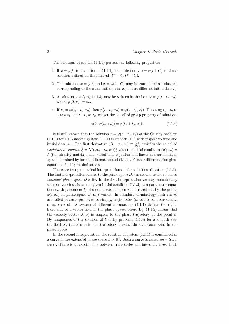
In the second interpretation, the solution of system (1.1.1) is considered as
a curve in the extended phase space D×R1. Such a curve is called an integral
curve. There is an explicit link between trajectories and integral curves. Each
1.1. Necessary background from the theory of ODEs 3
phase trajectory is the projection of a corresponding integral curve onto the
phase space along the t-axis, as depicted in Fig. 1.1.1. However, in contrast to
integral curves which are curves in the strict sense of the term, their projections
onto the phase space may no longer be curves but points. Such points are called
equilibrium states. They correspond to the constant solutions x = x∗. By
(1.1.2) X(x∗) = 0, i.e. equilibrium states are singular points of the vector field.
It is natural to pose the following question: can phase trajectories intersect each
other? This question is resolved by the following theorem.
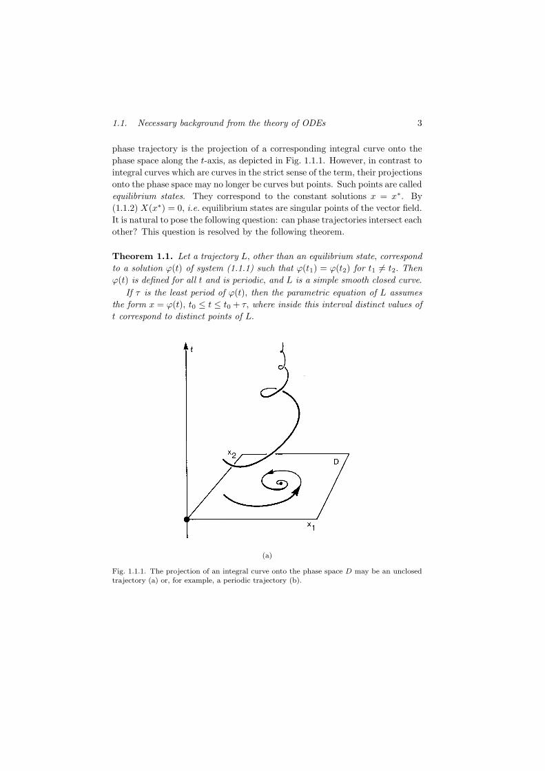
Theorem 1.1. Let a trajectory L, other than an equilibrium state, correspond
to a solution ϕ(t) of system (1.1.1) such that ϕ(t1) = ϕ(t2) for t1 6= t2. Then
ϕ(t) is defined for all t and is periodic, and L is a simple smooth closed curve.
If τ is the least period of ϕ(t), then the parametric equation of L assumes
the form x = ϕ(t), t0 ≤ t ≤ t0 + τ, where inside this interval distinct values of
t correspond to distinct points of L.
(a)
Fig. 1.1.1. The projection of an integral curve onto the phase space D may be an unclosed
trajectory (a) or, for example, a periodic trajectory (b).

4 Chapter 1. Basic Concepts
(b)
Fig. 1.1.1. (Continued)
For a proof of this theorem we refer the reader to the book Theory of Dy-
namical Systems on a Plane by Andronov, Leontovich, Gordon and Maier [6].
The trajectory L corresponding to a periodic solution ϕ(t) is called a
periodic trajectory.
Any other trajectory which is neither an equilibrium state nor a periodic
trajectory is an unclosed curve. It follows from Theorem 1.1 that an unclosed
trajectory has no points of self-intersection.
Note that any two solutions which differ from each other only in the choice
of the initial time t0 correspond to the same trajectory. Vice versa: any two
distinct solutions corresponding to the same trajectory are identical up to a
time shift t → t + C. It follows that all solutions corresponding to the same
periodic trajectory are periodic of the same period.
In the case where the solution corresponding to a given trajectory L is
defined for all t ∈ (−∞,+∞) we will say that L is an entire trajectory. Any
trajectory which lies in a bounded region is an entire trajectory.
From the view point of kinematics, the point ϕ(t) is called a representa-
tive point and its trajectory is called the associated motion. Moreover, for any

1.1. Necessary background from the theory of ODEs 5
trajectories other than equilibrium states, one can introduce a positive direc-
tion of the motion which points in the direction of increasing t. At each point of
such a trajectory this direction is determined by the associated tangent vector.
To emphasize this we will label all trajectories with arrowheads.
Along with system (1.1.1) let us consider an associated “time-reverse”
system
x = −X(x) . (1.1.5)
The vector field of system (1.1.5) is obtained from that of (1.1.1) by reversing
the direction of each tangent vector. It is easy to see that each solution x = ϕ(t)
of system (1.1.1) corresponds to a solution x = ϕ(−t) of system (1.1.5) and
vice versa. It is clear also that systems (1.1.1) and (1.1.5) have the same phase
curves up to a change of time t → −t. Thus, the time-oriented trajectories of
one system are obtained from the corresponding trajectories of the other by
reversing the direction of the arrowheads.
Consider next the system
x = X(x)f(x) , (1.1.6)
where the Cr-smooth function f(x) : D 7→ R
1 does not vanish in D. Observe
that systems (1.1.1) and (1.1.6) have the same phase curves which differ only
by time parametrization. Moreover, the trajectories of both systems have the
same directions if f(x) > 0, and opposite if f(x) < 0. If x = ϕ(t− t0, x0) is a
trajectory of (1.1.1) passing through x0 at x = x0, then parametrization of time
along this trajectory by the rule dt = dtf(ϕ(t−t0,x0))
or t = t0 +∫ t
t0ds
f(ϕ(s−t0,x0))
gives a trajectory of (1.1.6). We will call a transformation of such kind rescaling
of time or change of time.
Observe that in the case of system (1.1.1) we are interested only in the
form of the trajectory, there is no need to involve the independent variable t.
In this case we can consider the following more symmetric system
dx1
X1=dx2
X2= · · · =
dxnXn
.
If, for example, Xn is non-zero in a certain sub-region G ⊂ D, the form of the
trajectories in G may be found by solving the system
dxidxn
= XiX−1n .
This method is especially effective for studying two-dimensional systems.

6 Chapter 1. Basic Concepts
Generally speaking, not all trajectories may be continued over the infinite
interval τ = (−∞,+∞). In other words, not all trajectories are entire tra-
jectories.1 Examples of entire trajectories are equilibrium states and periodic
trajectories. From the point of view of dynamics, the entire trajectories, or
those which may be defined at least for all positive t over an infinite interval of
time, are of special interest. The reason is that, despite the importance of the
information revealed by transient solutions over a finite interval of time, the
most interesting phenomena observed in natural science and engineering ob-
tain an adequate explanation only if time t increases without bounds. Systems
whose solutions can be continued over an infinite period of time were named
dynamical systems by Birkhoff. An abstract definition of such systems which
takes into account their group properties, will be presented in the following
section.
1.2. Dynamical systems. Basic notions
Three components are used in the definition of a dynamical system. (1) A
metric space D called the phase space. (2) A time variable t which may be
either continuous, i.e. t ∈ R1, or discrete, i.e. t ∈ Z. (3) An evolution law,
i.e. a mapping of any given point x in D and any t to a uniquely defined state
ϕ(t, x) ∈ D which satisfies the following group-theoretic properties:
1. ϕ(0, x) = x .
2. ϕ(t1, ϕ(t2, x)) = ϕ(t1 + t2, x) .
3. ϕ(t, x) is continuous with respect to (x, t) .
(1.2.1)
In the case where t is continuous the above conditions define a continuous
dynamical system, or flow. In other words, a flow is a one-parameter group
of homeomorphisms2 of the phase space D. Fixing x and varying t from −∞
to +∞ we obtain an orientable curve3 as before, called a phase trajectory.
The following classification of phase trajectories is natural: equilibrium states,
periodic trajectories and unclosed trajectories. We will call x : ϕ(t, x), t ≥ 0
a positive semi-trajectory and x : ϕ(t, x), t ≤ 0 a negative semi-trajectory.
1There are systems whose solutions tend to infinity at some finite time. Such systemsare not dynamically defined systems.
2i.e. one-to-one, continuous mappings with continuous inverse. This follows directly fromthe group property (1.2.1) that ϕ(−t, ·) is inverse to ϕ(t, ·).
3The orientation is induced by the direction of motion.
1.2. Dynamical systems. Basic notions 7
Observe that in the case of an unclosed trajectory any point of the trajec-
tory partitions the trajectory into two parts: a positive semi-trajectory and a
negative semi-trajectory.
In the case where the mapping ϕ(t, x) is a diffeomorphism4 the flow is
a smooth dynamical system. In this case, the phase space D is endowed
with some additional smooth structures. The phase space D is usually cho-
sen to be either Rn, or R
n−k × Tk, where T
k may be a k-dimensional torus
S1 × S
1 × · · · × S1
︸ ︷︷ ︸
k times
, a smooth surface, or a manifold. This allows us to set up
a correspondence between a smooth flow and its associated vector field by
defining a velocity field
X(x) =dϕ(t, x)
dt
∣∣∣∣t=0
. (1.2.2)
By definition, the trajectories of the smooth flow are the trajectories of the
system x = X(x). In this book we will study mainly the properties of smooth
dynamical systems.
Discrete dynamical systems are often called cascades for simplicity. A
cascade possesses the following remarkable feature. Let us select a homeo-
morphism ϕ(1, x) and denote it by ψ(x). It is obvious that ϕ(t, x) = ψt(x),
where
ψt = ψ (ψ(· · ·ψ︸ ︷︷ ︸
t−1 times
(x))) .
Hence, in order to define a cascade it is sufficient to specify only the homeo-
morphism ψ : D 7→ D.
In the case of a discrete dynamical system the sequence xk+∞k=−∞ where
xk+1 = ψ(xk), is called a trajectory of the point x0. Trajectories may be of
three types:
1. A point x0. The point is a fixed point of the homeomorphism ψ(x), i.e. it
is mapped by ψ(x) into itself.
2. A cycle (x0, . . . , xk−1), where xi = ψi(x0), i = (0, . . . , k − 1) and x0 =
ψk(x0) moreover, xi 6= xj for i 6= j. The number k is called the period,
and each point xi is called a periodic point of period k. Observe that a
fixed point is a periodic point of period 1.
4A one-to-one, differentiable mapping with a differentiable inverse.
8 Chapter 1. Basic Concepts
3. A bi-infinite trajectory, i.e. a sequence xk+∞−∞, where k → ±∞, xi 6= xj
for i 6= j. In this case, as in the case of flows, we will say that such a
trajectory is unclosed.
When ψ(x) is a diffeomorphism, the cascade is a smooth dynamical system.
Examples of cascades of this type appear in the study of non-autonomous
periodic systems in the form
x = X(x, t) ,
where X(x, t) is continuous with respect to all variables in Rn×R
1, is smooth
with respect to x and periodic of period τ with respect to t. It is assumed
that the system has solutions which may be continued over the interval t0 ≤
t ≤ t0 + τ . Given a solution x = ϕ(t, x0), where ϕ(0, x0) = x0 we may define
a mapping
x1 = ϕ(τ, x) (1.2.3)
of the hyper-plane t = 0 into the hyper-plane t = τ . It follows from the
periodicity of X(x, t) that (X, t1) and (X, t2) must be identified if (t2 − t1) is
divisible by τ . Thus, (1.2.3) may be regarded as a diffeomorphism ψ : Rn →
Rn.5
Before proceeding further, we need to introduce some notions.
A set A is said to be invariant with respect to a dynamical system if
A = ϕ(t, A) for any t. Here, ϕ(t, A) denotes the set⋃
x∈A
ϕ(t, x). It follows from
this definition that if x ∈ A, then the trajectory ϕ(t, x) lies in A.
We call a point x0 wandering if there exists an open neighborhood U(x0)
of x0 and a positive T such that
U(x0) ∩ ϕ(t, U(x0)) = ∅ for t > T . (1.2.4)
Applying the transformation ϕ(−t, ·) to (1.2.4) we obtain
ϕ(−t, U(x0)) ∩ U(x0) = ∅ for t < T .
Hence, the definition of a wandering point is symmetric with respect to rever-
sion of time.
5Observe that system (1.2.3) may be written as an autonomous system
x = X(x, θ) , θ = 1 ,
where θ is taken in modulo τ .

1.2. Dynamical systems. Basic notions 9
Let us denote by W the set of wandering points. The set W is open and
invariant. Openness follows from the fact that together with x0 any point in
U(x0) is wandering. The invariance of W follows from the fact that if x0 is
a wandering point, then the point ϕ(t0, x0) is also a wandering point for any
t0. To show this let us choose ϕ(t0, U(x0)) to be a neighborhood of the point
ϕ(t0, x0). Then
ϕ(t0, U(x0)) ∩ ϕ(t, ϕ(t0, U(x0)) = ∅ for t > T .
Hence, the set of non-wandering points M = D\W is closed and invariant. The
set of non-wandering points may be empty. To illustrate the latter consider a
dynamical system defined by the autonomous system
x = X(x, θ) ,
θ = 1
in phase space Rn+1, x = (x1, . . . , xn). Observe that (1.2.4) holds here since
θ(t) = θ0 + t increases monotonically with t. Hence, every point in Rn+1 is a
wandering point.
It is clear that equilibrium states, as well as all points on periodic trajecto-
ries, are non-wandering. All points on bi-asymptotic trajectories which tend to
equilibrium states and periodic trajectories as t→ ±∞ are also non-wandering.
Such a bi-asymptotic trajectory is unclosed and called a homoclinic trajectory.
The points on Poisson-stable trajectories are also non-wandering points.
Definition 1.1. A point x0 is said to be positive Poisson-stable if given any
neighborhood U(x0) and any T > 0 there exists t > T such that
ϕ(t, x0) ⊂ U(x0) . (1.2.5)
If for any T > 0 there exists t such that t < −T and (1.2.5) holds, then the
point x0 is called a negative Poisson-stable point. If a point is positive and
negative Poisson stable it is said to be Poisson-stable.
Observe that if a point x0 is positive (negative) Poisson-stable, then any
point on the trajectory ϕ(t, x0) is also positive (negative) Poisson stable. Thus,
we may introduce the notion of a P+-trajectory (positive Poisson-stable), a
P−-trajectory (negative Poisson-stable) and merely a P -trajectory (Poisson-
stable). It follows directly from (1.2.5) that P+, P− and P -trajectories consist
of non-wandering points.

10 Chapter 1. Basic Concepts
It is obvious that equilibrium states and periodic trajectories are closed
P -trajectories.
Theorem 1.2. (Birkhoff)6 If a P+ (P−, P )-trajectory is unclosed, then its
closure Σ contains a continuum of unclosed P -trajectories.
Let us choose a positive sequence Tn where Tn → +∞ as n → +∞.
It follows from the definition of a P+-trajectory that there exists a sequence
tn → +∞ as n → +∞ such that ϕ(tn, x0) ⊂ U(x0). An analogous state-
ment holds in the case of a P−-trajectory. This implies that a P -trajectory
successively intersects any ε-neighborhood Uε(x0) of the point x0 infinitely
many times.7 Let tn(ε)+∞−∞ be chosen such that tn(ε) < tn+1(ε) and let
ϕ(tn(ε), x0) ⊂ Uε(x0). The values
τn(ε) = tn+1(ε) − tn(ε)
are called Poincare return times. Two essentially different cases are possible
for an unclosed P -trajectory:
1. The sequence τn(ε) is bounded for any finite ε, i.e. there exists a
number L(ε) such that τn(ε) < L(ε) for any n. Observe that L(ε) → +∞
as ε→ 0.
2. The sequence τn(ε) is unbounded for any sufficiently small ε.
In the first case the P -trajectory is called recurrent. For such a trajectory
all trajectories in its closure Σ are also recurrent, and the closure itself is
a minimal set.8 The principal property of a recurrent trajectory is that it
returns to an ε-neighborhood of the point x0 within a time not greater than
L(ε). However, in contrast to periodic trajectories, whose return times are
fixed, the return time for a recurrent trajectory is not constrained.
In the second case, the closure Σ of the P -trajectory is called a quasi-
minimal set. In this case, there always exist in Σ other invariant closed sub-
sets which may be equilibrium states, periodic trajectories, or invariant tori,
6See the proof in [14].7In the case of flows the set of times during which a P -trajectory passes through Uε(x0)
consists of infinitely many time intervals In(ε), where tn(ε) is chosen to be one of the valuesin In(ε).
8A set is called minimal if it is non-empty, invariant, closed and contains no propersubsets possessing these three properties.

1.2. Dynamical systems. Basic notions 11
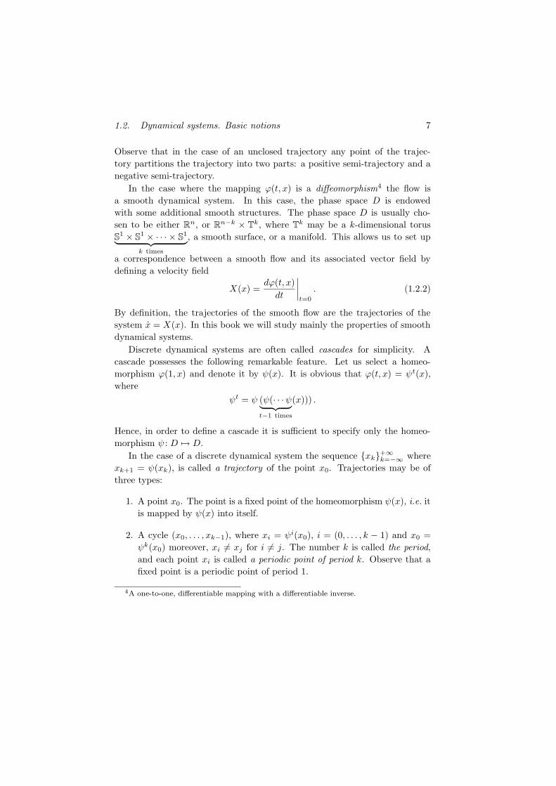
Fig. 1.2.1. The flow on a torus can be represented as a flow on the unit square. The slopeof all parallel trajectories is equal to ω2/ω1. Gluing the opposite sides of the square gives atwo-dimensional torus.
etc. Since a P -trajectory may approach such subsets arbitrarily closely, the
Poincare return times can therefore be arbitrarily large.
The simplest example of a flow all of whose trajectories are Poisson stable
is a quasi-periodic flow on a two-dimensional torus T2 defined by the equations
x1 = ω1 ,
x2 = ω2 ,(1.2.6)
where ω1/ω2 is irrational. This flow may be represented as a flow defined on
a unit rectangle with the points (x1, 0) and (x1, 1), and (0, x2) and (1, x2)
identified, as shown in Fig. 1.2.1. In this case, Σ = T2 is a minimal set, and
the flow possesses an unclosed trajectory which is everywhere dense on the
torus.9 When ω1/ω2 is rational, all trajectories of (1.2.6) on T2 are periodic.
Let f(x1, x2) be a function defined on the torus T2, i.e. f(x1 +1, x2 +1) =
f(x1 + 1, x2) = f(x1, x2). Assume also that f is smooth and vanishes at one
point (x01, x
02) only. The flow defined by the system
x1 = ω1f1(x1, x2) ,
x2 = ω2f2(x1, x2) ,
9This is called a quasi-periodic trajectory.

12 Chapter 1. Basic Concepts
on T2 is quasi-minimal. In this case Σ also coincides with T
2. However, Σ
contains an invariant subset which is the point (x01, x
02). All trajectories of
the flow on the torus are Poisson stable except for two trajectories: one tends
to (x01, x
02) as t → +∞, whereas another as t → −∞, respectively. We will
meet other examples of quasi-minimal sets in multi-dimensional autonomous
systems.
Let us introduce next the notion of an attractor.
Definition 1.2. An attractor A is a closed invariant set which possesses a
neighborhood (an absorbing domain) U(A) such that the trajectory ϕ(t, x) of
any point x in U(A) satisfies the condition
ρ((ϕ(t, x),A) → 0 as t→ +∞ , (1.2.7)
where
ρ(x,A) = infx0∈A
‖x− x0‖ .
The simplest examples of attractors are stable equilibrium states, sta-
ble periodic trajectories and stable invariant tori containing quasi-periodic
trajectories.
This definition of an attractor does not preclude the possibility that it may
contain other attractors. It is reasonable to restrict the notion of an attractor
by imposing a quasi-minimality condition. There exist a variety of attractors
which meet this condition. Of special interest among them are the so-called
strange attractors which are invariant closed sets comprised of only unstable
trajectories.
To conclude this section we remark that there are also systems in which
t ∈ R+ where R
+ denotes the non-negative half-line, or those in which t ∈
Z+ where Z
+ denotes the set of non-negative integers. In the former case a
dynamical system is defined by a semi-flow (semi-group), or by a non-invertible
mapping in the latter.
1.3. Qualitative integration of dynamical systems
The study of any phenomenon which exhibits dynamical behavior usually be-
gins with the construction of an associated mathematical model of a dynam-
ical system in the form (1.2.1). Having a model in an explicit form allows
us to follow the evolution of its state as time t varies, since the initial data
1.3. Qualitative integration of dynamical systems 13
defines a unique solution of (1.2.1). To undertake a complete study of the
model we must find this solution, i.e. “to integrate” the original system. “In-
tegrating a system” means obtaining an analytical expression for its solution.
However, this goal can be achieved only for a very small class of dynamical
systems; namely, for systems of linear equations with constant coefficients,
and for some very special equations which might be integrated in quadratures.
Moreover, even if the solution is given in analytical form, the component func-
tions which define the solution may be so complicated that a straightforward
analysis becomes practically impossible. Besides that, the problem of find-
ing an analytical form of a solution is not the primary goal of nonlinear dy-
namics, which is concerned mainly with such “qualitative” properties as the
number of equilibrium states, stability, the existence of periodic trajectories,
etc. Thus, following Poincare’s approach, instead of attempting a direct
integration of the differential equations, we try to extract information concern-
ing the character and form of the functions determined by these equations from
the equations themselves.10 More specifically, we seek to describe the impor-
tant qualitative features of these functions via a geometrical representation of
the phase trajectories. This is the reason why this method is called “qualitative
integration”.
The first step in our qualitative study is to identify all possible types of
trajectories having distinct behaviors and “forms”. The second step is to give
a description for each group of qualitatively similar trajectories. To achieve a
complete description it is necessary to identify certain more essential or “spe-
cial” trajectories. But here we run into a formidable problem: What properties
of the trajectories must we find in order to characterize the qualitative struc-
ture of the partition of the phase space into trajectories?
The first step is simple. In fact, it can be reformulated as follows: we must
find where a trajectory tends to as t→ +∞ (t→ −∞). Here, we must assume
that the trajectory L defined by x = ϕ(t) remains in some bounded region of
the phase space for t > t0 (t 6 t0). The following concepts are essential in this
study.
Definition 1.3. A point x∗ is called an ω-limit point of the trajectory L if
limk→∞
ϕ(tk) = x∗ ,
for some sequence tk where tk → +∞ as k → ∞.
10“Analyse des travans de Henri Poincare faite par lui-meme” [54].

14 Chapter 1. Basic Concepts
A similar definition of an α-limit point applies to tk → −∞ as k → ∞.
We denote the set of all ω-limit points of a trajectory L by ΩL, and that of
α-limit points by AL. Observe that an equilibrium state is the unique limit
point of itself. In the case where a trajectory L is periodic, all of its points are
α and ω-limit points, i.e. L = ΩL = AL. In the case where L is an unclosed
Poisson-stable trajectory, the sets ΩL and AL coincide with its closure L. The
set L is either a minimal set (if L is a recurrent trajectory) or a quasi-minimal
set if the Poincare return times of L are unbounded. All equilibrium states,
periodic trajectories, and Poisson-stable trajectories are said to be self-limit
trajectories.
The structure of the sets ΩL and AL has been more completely studied in
the case of two-dimensional dynamical systems where all trajectories remain
in some bounded domain of the plane as t → ±∞. In this case, Poincare
and Bendixson [13] had established that the set ΩL can only be of one of the
following three topological types:
I. Equilibrium states.
II. Periodic trajectories.
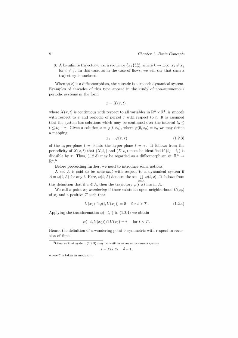
III. Cycles composed of equilibrium states and of connecting trajectories
which tend to these equilibrium states as t→ ±∞.
Figure 1.3.1 shows examples of limit sets of type III where the equili-
brium states are labeled by O. Using the general classification above, we
may enumerate all types of positive semi-trajectories in planar systems:
1. equilibrium states;
2. periodic trajectories;
3. semi-trajectories tending to an equilibrium state;
4. semi-trajectories tending to a periodic trajectory;
5. semi-trajectories tending to a limit set of type III.
An analogous situation occurs in the case of negative semi-trajectories. Among
periodic trajectories in the two-dimensional case a special role is assumed by
those which are either the ω-limit set, or the α-limit set of unclosed trajectories
located in the inner, or the outer domain of a periodic trajectory, as shown in

1.3. Qualitative integration of dynamical systems 15
(a)
(b)
(c)
Fig. 1.3.1. Examples of two ω-limit homoclinic cycles in (a) and (c), and of a heteroclinic
cycle in (b) formed by two trajectories going from one equilibrium state to another.
16 Chapter 1. Basic Concepts
(a)
(b)
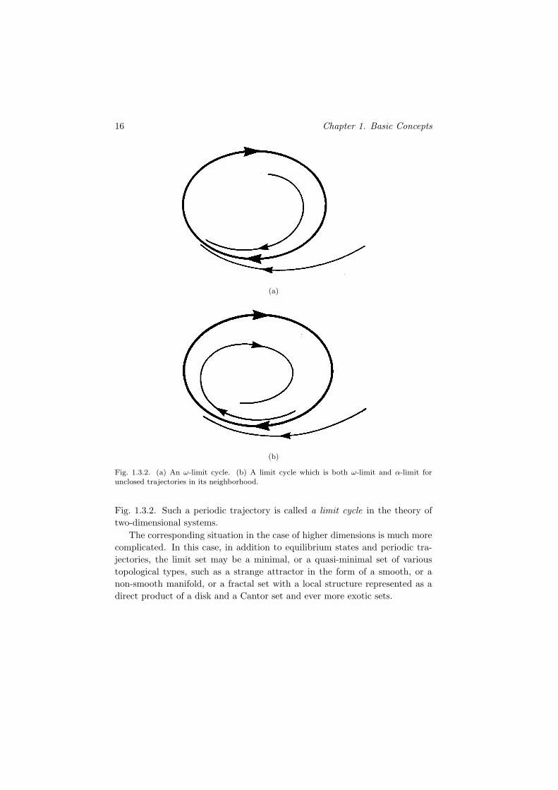
Fig. 1.3.2. (a) An ω-limit cycle. (b) A limit cycle which is both ω-limit and α-limit for
unclosed trajectories in its neighborhood.
Fig. 1.3.2. Such a periodic trajectory is called a limit cycle in the theory of
two-dimensional systems.
The corresponding situation in the case of higher dimensions is much more
complicated. In this case, in addition to equilibrium states and periodic tra-
jectories, the limit set may be a minimal, or a quasi-minimal set of various
topological types, such as a strange attractor in the form of a smooth, or a
non-smooth manifold, or a fractal set with a local structure represented as a
direct product of a disk and a Cantor set and ever more exotic sets.

1.3. Qualitative integration of dynamical systems 17
Let us now turn to the problem concerning the study of the totality of
trajectories. In fact, characterizing a dynamical system means topologically
(or qualitatively) partitioning the phase space into the region of the existence
of trajectories of different topological types. We usually refer to this problem
as “constructing the phase portrait”. This problem poses the question: When
are two phase portraits similar? In terms of the qualitative theory of dynamical
systems we can answer this question by introducing the notion of topological
equivalence.
Definition 1.4. Two systems are said to be topologically equivalent if there
exists a homeomorphism of the respective phase spaces which maps the trajec-
tories of one system into the trajectories of the second.11
This definition implies that equilibrium states, as well as periodic and un-
closed trajectories of one system, are respectively mapped into equilibrium
states, as well as periodic and unclosed trajectories of the other system. The
topological equivalence of two systems in some sub-regions of the phase space
is defined in a similar manner. The latter is usually used for studying local
problems, for example, in a neighborhood of an equilibrium state, or near pe-
riodic or homoclinic trajectories. The definition of topological equivalence of
two dynamical systems gives an indirect definition of the qualitative structure
of partition of the phase space into the regions of the existence of trajectories
of topologically different types. Such structures must be invariant with respect
to all possible homeomorphisms of the phase space.
Let G be a bounded sub-region of the phase space and let H = hi be a
set of homeomorphisms defined on G. We can introduce a metric as follows
dist(h1, h2) = supx∈G
‖h1x− h2x‖ .
Definition 1.5. We call a trajectory L, L ∈ G, special if for a sufficiently
small ε > 0, for all homeomorphisms hi satisfying dist(hi, I) < ε, where I is
the identity homeomorphism, the following condition holds
hiL = L .
It is clear that all equilibrium states and periodic trajectories are special
trajectories. Unclosed trajectories may also be special. For example, all tra-
jectories of a two-dimensional system which tend to saddle equilibrium states
11See Sec. 2.5 for details.

18 Chapter 1. Basic Concepts
both as t→ +∞ and as t→ −∞ are also special trajectories. Since such tra-
jectories separate certain regions in the plane they are called separatrices (see
examples of separatrices in Fig. 1.3.1). A definition for special semi-trajectories
may be introduced in an analogous way.
Definition 1.6. Two trajectories L1 and L2 are said to be equivalent if given
ε > 0, there exist homeomorphisms h1, h2, . . . , hm(ε) such that
L2 = hm(ε) · · ·h1L1 .
where dist(hk, I) < ε (k = 1, 2, . . . ,m(ε)).
We will call each set of equivalent trajectories a cell. Observe that all
trajectories in a cell are of the same topological type. In particular, if a cell is
composed of unclosed trajectories, then all of them have the same ω-limit set
and the same α-limit set.
Special trajectories and cells are especially important for two-dimensional
systems. In this case we may identify some set S by selecting a single trajectory
from each cell (all special trajectories belong to S by definition). We will call
this set S a scheme.12
Let us assume that S consists of a finite number of trajectories.13
Theorem 1.3. The scheme is a complete topological invariant.
This theorem, together with its proof, occupies a significant part of the book
Theory of Dynamical Systems on the Plane by Andronov, Leontovich, Gordon
and Maier [6]. This theory provides not only a mathematical foundation for a
theory of oscillations of two-dimensional systems but also gives a recipe for the
investigation of concrete systems. In particular, the investigation proceeds in
the following order: First, classify the equilibrium states, and then all special
trajectories such as separatrices tending to saddle equilibria and trajectories
approaching limit sets of type III, either as t → +∞, or as t → −∞. This
entire collection of special trajectories determines a schematic portrait called
a skeleton which allows one to partition the phase space into cells, as well as
to study the behavior of the trajectories within each cell.
Unfortunately, this does not work when we examine systems of higher
dimensions. The set of special trajectories in a three-dimensional system may
12The set S can be considered as a factor-system with respect to the above equivalencerelation.
13The finiteness condition of S is rather general, holding for a wide class of planar systems.

1.3. Qualitative integration of dynamical systems 19
already be infinite, or may even form a continuum. The same situation applies
to cells. Thus, the problem of finding a complete topological invariant in this
case seems to be quite unrealistic. This is the reason why we must reconcile to
the concept of a relatively-incomplete classification based on some topological
invariants which apply only to certain cases. Nevertheless, the basic approach
for studying concrete high-dimensional systems remains the same as in
the two-dimensional case; namely, it begins by examining the equilibrium
states and the periodic trajectories. We will consider this “comprehensive”
local theory in Chaps. 2 and 3, respectively.

Chapter 2
STRUCTURALLY STABLE EQUILIBRIUM
STATES OF DYNAMICAL SYSTEMS
2.1. Notion of an equilibrium state. A linearizedsystem
Let us consider a system of differential equations
x = X(x) (2.1.1)
where x ∈ Rn and X is a smooth function in some region D ⊂ R
n.
Definition 2.1. A trajectory x(t) of system (2.1.1) is called an equilibrium
state if it does not depend on time, i.e. x(t) ≡ x0 = const.
It follows from the definition that the coordinates of the equilibrium state
can be found as the solution of the system:
X(x0) = 0 . (2.1.2)
If the Jacobian matrix ∂X/∂x is non-singular at the point x0, then, by virtue
of the implicit function theorem, there are no other solutions of Eq. (2.1.2)
nearby x0. This means that the equilibrium state is isolated. However, even
when the Jacobian matrix is singular the equilibrium state is usually isolated
(excluding the case where the right-hand side of X(x) is of a very special type).
Thus, in the general case system (2.1.1) has only a finite number of equilibrium
states in any bounded subregion of Rn. Furthermore, when the right-hand side
21

22 Chapter 2. Structurally Stable Equilibrium States of Dynamical Systems
of (2.1.1) is polynomial there are standard algebraic methods for the evaluation
of the number of equilibrium states.
From the point of view of numerical simulations the determination of all
isolated solutions of system (2.1.2) (or equivalently of all stationary states of
(2.1.1)) in a bounded subregion of Rn is a relatively simple task for small n.
However, the number of equilibrium states of a system of higher dimension may
be very large and therefore searching for all of them becomes problematic.
The study of system (2.1.1) near an equilibrium state is based on a standard
linearization procedure.
Let a point O(x = x0) be an equilibrium state of system (2.1.1). The
substitution
x = x0 + y (2.1.3)
shifts the origin to O. With the new variables the system may be written as
y = X(x0 + y) , (2.1.4)
or, by Taylor expansion near x = x0, as
y = X(x0) +∂X(x0)
∂xy + o(y) . (2.1.5)
Since X(x0) = 0 system (2.1.5) becomes
y = Ay + g(y) , (2.1.6)
where
A =∂X(x0)
∂x;
A is a constant (n× n)-matrix and g(y) satisfies the condition
g(0) =∂g(0)
∂y= 0 . (2.1.7)
In the general case, the last term in (2.1.6) is of a higher order of smallness
(with respect to the usual norm) than the first term. It is apparent that the
behavior of the trajectories of system (2.1.6) in a small neighborhood of the
origin is governed primarily by the linearized system
y = Ay . (2.1.8)
The study of linear systems was the major paradigm of non-conservative
dynamics in the 19th century and at the beginning of the 20th century. The

2.1. Notion of an equilibrium state. A linearized system 23
main source of such systems was the theory of automatic control, in particular,
the control theory of steam engines. The central problem of linear dynamics
in that period was the search for the most effective criteria of stability for
stationary states.1
The stability of an equilibrium state is determined by the eigenvalues
(λ1, . . . , λn) of the Jacobian matrix A which are the roots of the character-
istic equation
det |A− λI| = 0 (2.1.9)
where I is the identity matrix. The roots of the characteristic equation are also
called the characteristic exponents of the equilibrium state. The equilibrium
state is stable when all of its characteristic exponents lie in the left half-plane
(LHP) on the complex plane. Moreover, any deviations from equilibrium de-
cay exponentially with decrements of damping proportional to the values Reλi,
(i = 1, . . . , n). Thus, the primary problem of constructing a simple and effec-
tive criterion of the stability of an equilibrium state was in finding some explicit
conditions in terms of the entries of the matrix A such that it would allow one
to determine, without having to solve the characteristic equation, when all of
its eigenvalues lie in open LHP.
Here, we present the most popular algorithm called a Routh–Hurwitz cri-
terion. Let (a0, . . . , an) be the coefficients of the polynomial det |λI −A|:
det |λI −A| = a0λn + a1λ
n−1 + · · · + an .
We construct an (n× n)-matrix:
A =
∣∣∣∣∣∣∣∣∣∣∣∣∣∣∣∣
a1 a3 a5 · · · 0 0
a0 a2 a4 · · · 0 0
0 a1 a3 · · · 0 0
0 a0 a2 · · · 0 0...
......
. . .. . .
...
0 0 0 · · · an−1 0
0 0 0 · · · an−2 an
∣∣∣∣∣∣∣∣∣∣∣∣∣∣∣∣
(2.1.10)
and find the minors ∆1 = a1, ∆2 = a1a2 − a0a3, . . . , ∆n = det A. Here, ∆i is
the determinant of the matrix whose entries lie on the intersection of the first
i rows and the first i columns of the matrix A.
1The necessity for studying nonlinear nonconservative systems emerged only in the firstpart of the 20th century, in the context of the investigation of the phenomenon of sustainedoscillations in vacuum-tube oscillators.

24 Chapter 2. Structurally Stable Equilibrium States of Dynamical Systems
Routh Hurwitz criterion. All characteristic exponents have negative
real parts if and only if each ∆i is positive.
The mathematical question of the correspondence between the properties
of the nonlinear system near the equilibrium state and those of the associated
linearized system was first posed in papers by Poincare and Lyapunov. This
problem has now been resolved to a considerable extent. In the following
sections we will study it in detail and describe the behavior of trajectories of
nonlinear systems in a neighborhood of their structurally stable (equiv. rough)
equilibrium states, i.e. those which have no characteristic exponents with zero
real part. We note that the presentation below differs from the usual treatment
in the sense that we will focus on those features of the system which one needs
for the study of strange attractors containing saddle equilibrium states, for
example, the Lorenz attractor, the spiral attractors, double-scroll attractors in
the Chua circuit, etc.
2.2. Qualitative investigation of 2- and 3-dimensionallinear systems
In this and in the following two sections we will study the behavior of solutions
of the linearized system. Moreover, we will restrict ourselves to structurally
stable equilibrium states only.
Let us begin with low dimensional cases n = 2 and n = 3.
When n = 2 the system assumes this general form:
x = a11x+ a12y ,
y = a21x+ a22y .(2.2.1)
The corresponding characteristic equation is
λ2 − (a11 + a22)λ+ (a11a22 − a12a21) = 0 (2.2.2)
and its roots are
λ1,2 = (a11 + a22)/2 ±√
(a11 + a22)2/4 − (a11a22 − a12a21) .
The names of the basic equilibrium states of two-dimensional systems were
first given by Poincare. They depend on the values of the characteristic expo-
nents λ1,2 as follows:
2.2. Qualitative investigation of linear systems 25
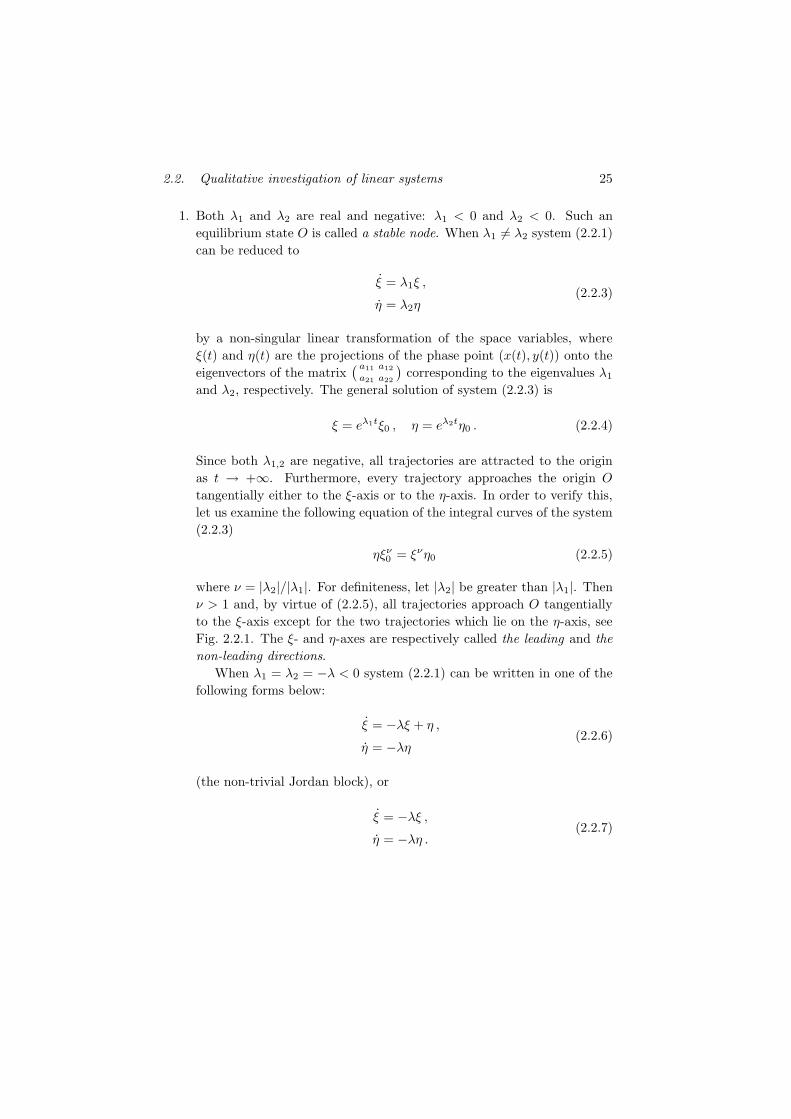
1. Both λ1 and λ2 are real and negative: λ1 < 0 and λ2 < 0. Such an
equilibrium state O is called a stable node. When λ1 6= λ2 system (2.2.1)
can be reduced to
ξ = λ1ξ ,
η = λ2η(2.2.3)
by a non-singular linear transformation of the space variables, where
ξ(t) and η(t) are the projections of the phase point (x(t), y(t)) onto the
eigenvectors of the matrix( a11 a12
a21 a22
)corresponding to the eigenvalues λ1
and λ2, respectively. The general solution of system (2.2.3) is
ξ = eλ1tξ0 , η = eλ2tη0 . (2.2.4)
Since both λ1,2 are negative, all trajectories are attracted to the origin
as t → +∞. Furthermore, every trajectory approaches the origin O
tangentially either to the ξ-axis or to the η-axis. In order to verify this,
let us examine the following equation of the integral curves of the system
(2.2.3)
ηξν0 = ξνη0 (2.2.5)
where ν = |λ2|/|λ1|. For definiteness, let |λ2| be greater than |λ1|. Then
ν > 1 and, by virtue of (2.2.5), all trajectories approach O tangentially
to the ξ-axis except for the two trajectories which lie on the η-axis, see
Fig. 2.2.1. The ξ- and η-axes are respectively called the leading and the
non-leading directions.
When λ1 = λ2 = −λ < 0 system (2.2.1) can be written in one of the
following forms below:
ξ = −λξ + η ,
η = −λη(2.2.6)
(the non-trivial Jordan block), or
ξ = −λξ ,
η = −λη .(2.2.7)

26 Chapter 2. Structurally Stable Equilibrium States of Dynamical Systems
Fig. 2.2.1. A stable node. Double arrows label the strongly stable (non-leading)direction which coincides with the η-axis.
The general solution of the system (2.2.6) is given by
ξ = e−λtξ0 + te−λtη0 , η = e−λtη0 (2.2.8)
and that of the system (2.2.7) is given by
ξ = e−λtξ0 , η = e−λtη0 . (2.2.9)
Figure 2.2.2 shows the phase portrait in the first case. All trajectories
tend to O tangentially to the unique eigenvector, namely, the ξ-axis. In
the second case any trajectory approaches O along its own eigen-direction
as shown in Fig. 2.2.3. Such a node is called a dicritical node.
2. A pair of complex-conjugate roots: λ1,2 = −ρ ± iω, ρ > 0, ω > 0. In this
case the equilibrium state O is called a stable focus. By a non-singular
linear change of coordinates the system (2.2.1) can be transformed into:
ξ = −ρξ − ωη ,
η = ωξ − ρη .(2.2.10)

2.2. Qualitative investigation of linear systems 27
Fig. 2.2.2. Another stable node. Every trajectory enters the origin along the onlyleading direction which is the ξ-axis.
Fig. 2.2.3. A dicritical node. Every trajectory tends to O along its own direction.
28 Chapter 2. Structurally Stable Equilibrium States of Dynamical Systems
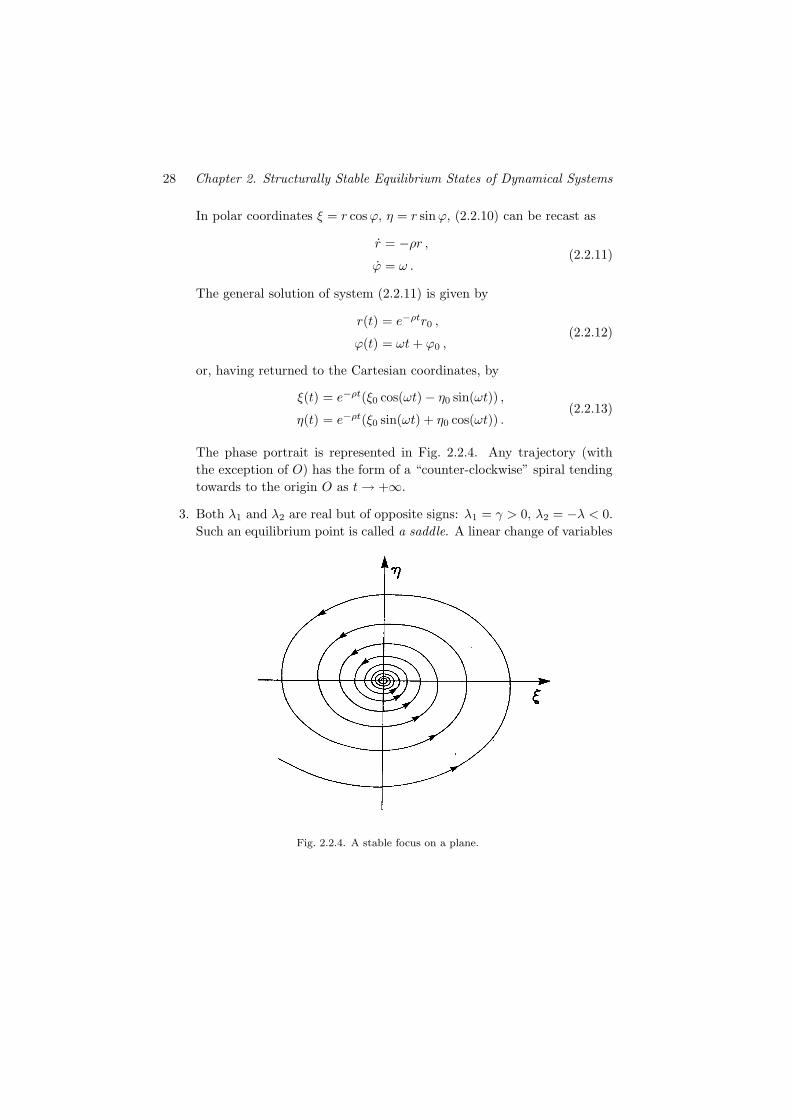
In polar coordinates ξ = r cosϕ, η = r sinϕ, (2.2.10) can be recast as
r = −ρr ,
ϕ = ω .(2.2.11)
The general solution of system (2.2.11) is given by
r(t) = e−ρtr0 ,
ϕ(t) = ωt+ ϕ0 ,(2.2.12)
or, having returned to the Cartesian coordinates, by
ξ(t) = e−ρt(ξ0 cos(ωt) − η0 sin(ωt)) ,
η(t) = e−ρt(ξ0 sin(ωt) + η0 cos(ωt)) .(2.2.13)
The phase portrait is represented in Fig. 2.2.4. Any trajectory (with
the exception of O) has the form of a “counter-clockwise” spiral tending
towards to the origin O as t→ +∞.
3. Both λ1 and λ2 are real but of opposite signs: λ1 = γ > 0, λ2 = −λ < 0.
Such an equilibrium point is called a saddle. A linear change of variables
Fig. 2.2.4. A stable focus on a plane.

2.2. Qualitative investigation of linear systems 29
brings the system (2.2.1) to the form
ξ = γξ ,
η = −λη .(2.2.14)
The general solution of the system (2.2.14) is given by
ξ = eγtξ0 , η = e−λtη0 . (2.2.15)
The corresponding equation of integral curves is given by
ηξν = ξν0η0 , (2.2.16)
where ν = λ/γ. The portrait of the phase space (or just “the phase
space”) near the saddle is shown in Fig. 2.2.5. There are four exclusive
trajectories called the separatrices, two stable and two unstable, which
tend to the saddle O as t→ +∞ and as t→ −∞ respectively. All other
trajectories pass by the saddle. The pair of the stable separatrices to-
gether with the saddle O compose the stable invariant subspace of the
Fig. 2.2.5. A planar saddle.

30 Chapter 2. Structurally Stable Equilibrium States of Dynamical Systems
saddle (the η-axis). The unstable invariant subspace of the saddle
(the ξ-axis) consists of the unstable separatrices and of the saddle
point.
4. The case where the real parts of both characteristic exponents are positive
can be simply reduced to the cases (1) and (2) above by the change
of time t → −t, so that the directions of the arrows in the respective
phase portraits are reversed. When the characteristic exponents are real,
the associated equilibrium state is called an unstable node. In the case
of complex characteristic exponents it is called an unstable focus (see
Figs. 2.2.6 and 2.2.7).
5. Let us now consider the equilibrium states of three-dimensional systems.
Consider first the case where the characteristic exponents λi (i = 1, 2, 3)
are real and λ3 < λ2 < λ1 < 0. Then, the associated three-dimensional
system may be reduced to the form
x = λ1x , y = λ2y , z = λ3z . (2.2.17)
Fig. 2.2.6. An unstable node. The picture is obtained from Fig. 2.2.1 by reversingthe time.

2.2. Qualitative investigation of linear systems 31
Fig. 2.2.7. An unstable focus. A trajectory traces out a “clockwise” spiral on theplane.
Its general solution is given by
x = eλ1tx0 , y = eλ2ty0 , z = eλ3tz0 . (2.2.18)
Since all λi’s are negative, the point O is a stable equilibrium state, i.e. all
trajectories tend to O as t → +∞. Furthermore, all trajectories outside
of the non-leading plane (y, z) approach O along the leading direction
that coincides with the x-axis, see Fig. 2.2.8. Such an equilibrium state
is called a stable node.
Let us now consider the case where among the characteristic expo-
nents there is a pair of complex-conjugate λ2,3 = −ρ± iω. The equilib-
rium state of the system
x = λ1x , y = −ρy − ωz , z = ωy − ρz (2.2.19)
in the case where −ρ < λ1 < 0, O is also called a stable node. The
general solution has the form
x(t) = eλ1tx0 ,
y(t) = e−ρt(y0 cos(ωt) − z0 sin(ωt)) ,
z(t) = e−ρt(y0 sin(ωt) + z0 cos(ωt)) .
(2.2.20)

32 Chapter 2. Structurally Stable Equilibrium States of Dynamical Systems
Fig. 2.2.8. A stable node in R3. The fewer the arrows the weaker is the rate ofcontraction. The leading subspace EL is one-dimensional, two-dimensional subspaceEss is non-leading.
(see (2.2.13)). The phase portrait of this system is shown in Fig. 2.2.9.
It follows from (2.2.20) that
√
y(t)2 + z(t)2 = e−ρt√
y20 + z2
0 .
Moreover, for any trajectory whose initial point does not lie in the
non-leading plane (y, z), we obtain
√
y(t)2 + z(t)2 = C|x(t)|ν (2.2.21)
where ν = ρ/|λ1| and C =√
y20 + z2
0/|x0|ν . Since ν > 1, all such trajec-
tories approach O along the leading x-axis.
6. When λ1 < −ρ < 0 the equilibrium state of system (2.2.19) is called a
stable focus. Relation (2.2.21) still holds, but as ν < 1, all trajectories
for which C 6= 0 (i.e. having initial points which are not on the x-axis)
tend to O tangentially to the plane (y, z) as shown in Fig. 2.2.10. In this
case, the x-axis is called the non-leading direction and the (y, z)-plane is
the leading plane, respectively.

2.2. Qualitative investigation of linear systems 33
Fig. 2.2.9. Another possible stable node in R3. Although the point O is a stablefocus on Ess, all trajectories outside Ess go to O along the one-dimensional leadingsubspace EL.
Fig. 2.2.10. A stable focus in R3. In contrast to Fig. 2.2.9, all trajectories outsideof the one-dimensional subspace Ess tend to O tangentially to the two-dimensionalleading subspace EL.

34 Chapter 2. Structurally Stable Equilibrium States of Dynamical Systems
7. When all characteristic exponents lie to the right of the imaginary axis
(i.e. in the open right-half plane (RHP)), by reversion of time t→ −t, we
reduce the problem to the cases considered above. Here, all trajectories
tend to the equilibrium state as t→ −∞. As before, there exist two kinds
of equilibrium states, namely: an unstable node, if the characteristic
exponent nearest to the imaginary axis is real, and an unstable focus,
when the characteristic exponents nearest to the imaginary axis comprise
a complex-conjugate pair. The corresponding phase portraits are similar
to those shown in Figs. 2.2.8–2.2.10 but with all the arrows pointing in
the opposite direction.
8. If there are characteristic exponents both to the left and to the right of
the imaginary axis, the equilibrium state is either a saddle or a saddle-
focus (this name was also given by Poincare), see Figs. 2.2.11–2.2.14.
Let us assume that λ1 > 0 and λs < 0, (s = 2, 3) in (2.2.17). Then,
the equilibrium state of system (2.2.17) is a saddle, see Fig. 2.2.11.
The general solution is also given by (2.2.18). Because λ1 > 0, λ2 < 0,
λ3 < 0, the coordinates y and z decay exponentially to zero as t→ +∞
Fig. 2.2.11. A saddle O with the two-dimensional stable subspace Es and the one-
dimensional unstable subspace Eu.

2.2. Qualitative investigation of linear systems 35
Fig. 2.2.12. A saddle (1,2).
Fig. 2.2.13. A saddle-focus (2,1). It has a two-dimensional stable subspace Es and a
one-dimensional unstable subspace Eu.
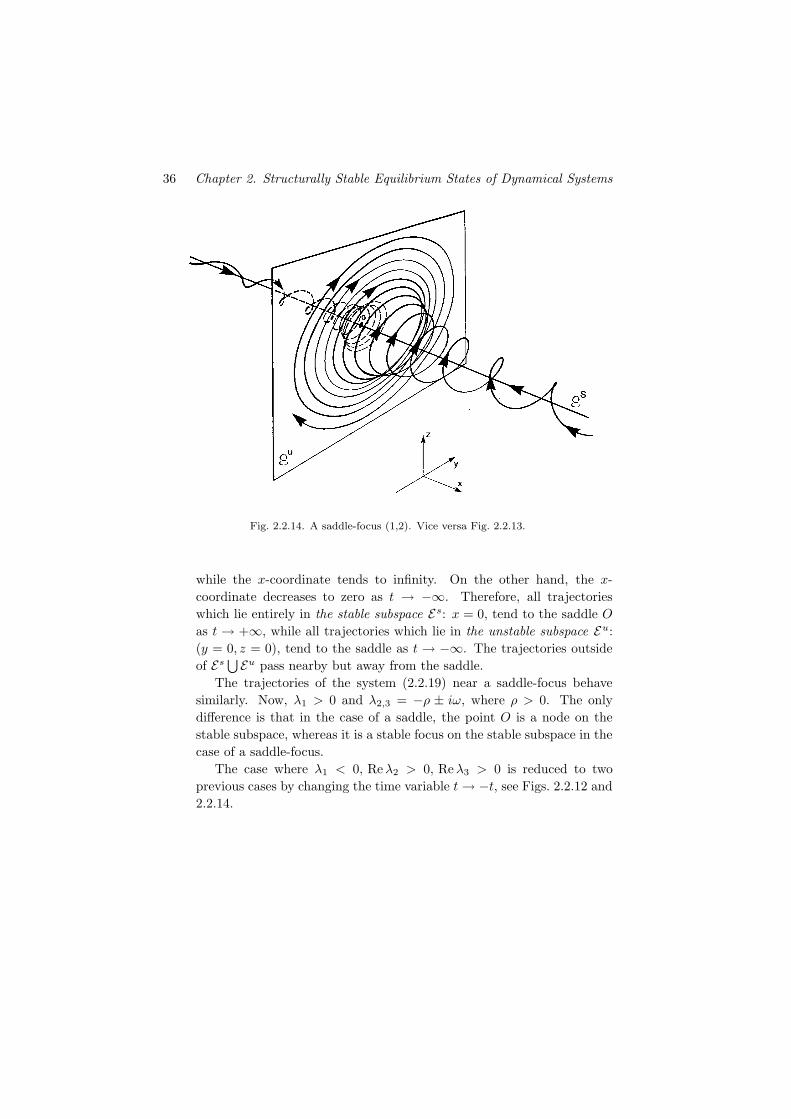
36 Chapter 2. Structurally Stable Equilibrium States of Dynamical Systems
Fig. 2.2.14. A saddle-focus (1,2). Vice versa Fig. 2.2.13.
while the x-coordinate tends to infinity. On the other hand, the x-
coordinate decreases to zero as t → −∞. Therefore, all trajectories
which lie entirely in the stable subspace Es: x = 0, tend to the saddle O
as t → +∞, while all trajectories which lie in the unstable subspace Eu:
(y = 0, z = 0), tend to the saddle as t → −∞. The trajectories outside
of Es⋃Eu pass nearby but away from the saddle.
The trajectories of the system (2.2.19) near a saddle-focus behave
similarly. Now, λ1 > 0 and λ2,3 = −ρ ± iω, where ρ > 0. The only
difference is that in the case of a saddle, the point O is a node on the
stable subspace, whereas it is a stable focus on the stable subspace in the
case of a saddle-focus.
The case where λ1 < 0, Reλ2 > 0, Reλ3 > 0 is reduced to two
previous cases by changing the time variable t→ −t, see Figs. 2.2.12 and
2.2.14.

2.3. High-dimensional linear systems. Invariant subspaces 37
2.3. High-dimensional linear systems. Invariantsubspaces
Let us consider the system
y = Ay , (2.3.1)
where y ∈ Rn. The general solution is given by
y(t) = eAty0 . (2.3.2)
Recall that the exponential eB of a matrix B is defined as the sum of the matrix
series
eB = I +B +B2/2 + · · · +Bk/k! + · · · ,
here and below I denotes the identity matrix. Thus, the general solution of
the system (2.3.1) can be rewritten as
y(t) = (I +At+A2t2/2 + · · · +Aktk/k! + · · · )y0 . (2.3.3)
The convergence of the series (2.3.3) for any t is obvious since ‖Aktk/k!‖ does
not exceed ‖A‖k|t|k/k! which decays very fast as k → ∞. To verify that (2.3.3)
is the general solution, we should note from (2.3.3) that
y(0) = y0
and
y(t) = (A+A2t+ · · · +Aktk−1/(k − 1)! + · · · )y0
= A(I +At+A2t2/2 + · · · +Ak−1tk−1/(k − 1)! + · · · )y0 = Ay(t) .
Let us elaborate the expression (2.3.2). If all eigenvalues of the matrix A are
real and different, then one may choose the eigen-basis as a coordinate frame
such that matrix A becomes diagonal, i.e.
A =
λ1 0λ2
. . .
0 λn
,
where we have abused our notation by using the same symbol A to denote the
original matrix in the new basis to avoid clutter. In this basis we have
Ak =
λk1 0λk2
. . .
0 λkn

38 Chapter 2. Structurally Stable Equilibrium States of Dynamical Systems
and, therefore
eAt =
eλ1t 0eλ2t
. . .
0 eλnt
.
Thus, if we denote the components of the vector y ∈ Rn by (y1, . . . , yn) in the
given basis, then the solution of the system can be rewritten in the form:
ys(t) = eλstys0 , (s = 1, . . . , n) . (2.3.4)
If all eigenvalues (we will also call them the characteristic exponents) are
different as before, but some of them are complex, then there exists a basis in
which A attains a block-diagonal form:
A1 0A2
. . .
0 Am
, (2.3.5)
where each block Aj corresponds to either a real eigenvalue, or to a pair of
complex-conjugate eigenvalues (recall that if A is the real matrix, then the
complex-conjugate λ∗i of any complex eigenvalue λi is also an eigenvalue). If
λj is real, its corresponding block is a (1 × 1)-matrix:
Aj = (λj) . (2.3.6)
If λ = ρ + iω and λ∗ = ρ − iω are a pair of complex-conjugate eigenvalues,
then the corresponding block is a (2 × 2)-matrix:
Aj =
(ρ −ω
ω ρ
)
=
(Reλ −Imλ
Imλ Reλ
)
. (2.3.7)
In this basis
Ak =
Ak1 0Ak2
. . .
0 Akm
.
Furthermore, for the complex λ we have
Akj =
(Re (λk) −Im (λk)
Im (λk) Re (λk)
)
,

2.3. High-dimensional linear systems. Invariant subspaces 39
hence we obtain
eAt =
eA1t 0eA2t
. . .
0 eAmt
,
where
eAjt =
eλt for Aj = (λ)
(Re eλt −Im eλt
Im eλt Re eλt
)
= eρt(
cos(ωt) − sin(ωt)
sin(ωt) cos(ωt)
)
for Aj =
(ρ −ω
ω ρ
)
.
So, the general solution (2.3.2) has the form
ys(t) = eλst ys0 (2.3.8)
for real λs and
ys(t) = eρt(ys0 cos(ωt) − ys+1,0 sin(ωt)) (2.3.9)
ys+1(t) = eρt(ys0 sin(ωt) + ys+1,0 cos(ωt)) (2.3.10)
for complex λs = λ∗s+1 = ρ+ iω.
If A has some multiple eigenvalues one may make a linear transformation
so that A becomes block-diagonal in a Jordan basis. Blocks corresponding to
simple eigenvalues remain unchanged from the previous case, but for each real
eigenvalue λ of multiplicity k, the corresponding block is a (k × k)-matrix of
the form
λ δ1 0λ δ2
λ. . .. . .
. . .
. . . δk−1
0 λ
, (2.3.11)

40 Chapter 2. Structurally Stable Equilibrium States of Dynamical Systems
where δi is either 0 or 1. For each pair of complex-conjugate eigenvalues of
multiplicity k, the corresponding block is a (2k × 2k)-matrix of the form
Λ δ1 I 0Λ δ2 I
Λ.. .. . .
. . .
. . . δk−1 I0 Λ
, (2.3.12)
where the matrix Λ is given by (2.3.7), I is the (2 × 2) identity matrix and δiis either 0 or 1. In this case y(t) can also be easily found from formula (2.3.3).
For the coordinates ys corresponding to simple eigenvalues, formulae (2.3.12)
and (2.3.13) and (2.3.10) remain unchanged.
For coordinates (yi+1, . . . , yi+k) corresponding to a real eigenvalue λ of
multiplicity k in the case of the complete Jordan block (i.e. when all δ’s in
(2.3.15) are equal to 1) the following formulae are valid:
yi+k(t) = eλtyi+k,0 ,
yi+k−1(t) = eλt(yi+k−1,0 + tyi+k,0) ,
......
...
yi+j(t) = eλts=k∑
s=j
yi+s,0ts−j
(s− j)!,
......
...
(2.3.13)
or, equivalently,
(yi+1(t), . . . , yi+k(t)) = eλt(yi+1,0, . . . , yi+k,0)eJkt , (2.3.14)
where Jk denotes the (k × k)-matrix
0 01 0
1 0. . .
. . .
. . .. . .
0 1 0
(this is the transposed non-diagonal part of (2.3.15)).

2.3. High-dimensional linear systems. Invariant subspaces 41
For coordinates (yi+1, . . . , yi+2k), corresponding to a pair of the complex-
conjugate eigenvalues of multiplicity k in the case of the complete Jordan block,
we have
yi+2j−1(t) = eρts=k∑
s=j
(yi+2s−1,0 cos(ωt) − yi+2s,0 sin(ωt))ts−j/(s− j)! ,
yi+2j(t) = eρts=k∑
s=j
(yi+2s−1,0 sin(ωt) + yi+2s,0 cos(ωt))ts−j/(s− j)!
(2.3.15)
or, equivalently
(yi+1 (t) · · · yi+2k−1 (t)
yi+2 (t) · · · yi+2k (t)
)
= eΛt(yi+1,0 · · · yi+2k−1,0
yi+2,0 · · · yi+2k,0
)
eJkt ,
(2.3.16)
where Λ is matrix (2.3.7), Jk is the same as in (2.3.14).
If λ is real and the Jordan block is not complete, i.e. in (2.3.15) some
δj vanish, then the block corresponding to λ may be partitioned into two
sub-blocks as follows
λ δ1 0 |
λ. . . |. . . δj−1 | 0
0 λ |− − − − | − − − −
| λ δj+1 0
0 | λ. . .
|. . . δk
| 0 λ
and the exponential is separately found for each sub-block. Analogous calcu-
lations are carried out for each complex eigenvalue λ of multiplicity k with a
non-complete Jordan block.
We can now prove the following lemma which gives a standard estimate
for the norm of the exponential matrix. This estimate will be frequently used
throughout the book.

42 Chapter 2. Structurally Stable Equilibrium States of Dynamical Systems
Lemma 2.1. For given an arbitrarily small ε > 0, one can choose an appro-
priate basis in Rn such that the solution y(t) = eAty0 of the linear system
y = Ay
satisfies the following inequalities
‖y(t)‖ ≤ ‖eAt‖ ‖y0‖ ≤ e(max Reλi+ε)t ‖y0‖ for t ≥ 0 ; (2.3.17)
‖y(t)‖ ≥ ‖e−At‖−1 ‖y0‖ ≥ e(min Reλi−ε)t ‖y0‖ for t ≥ 0 ; (2.3.18)
‖y(t)‖ ≤ ‖eAt‖ ‖y0‖ ≤ e(min Reλi−ε)t ‖y0‖ for t ≤ 0 ; (2.3.19)
‖y(t)‖ ≥ ‖e−At‖−1 ‖y0‖ ≥ e(max Reλi+ε)t ‖y0‖ for t ≤ 0 , (2.3.20)
where λi (i = 1, . . . , n) are the characteristic exponents of the matrix A and the
norm ‖ · ‖ of the vector y ∈ Rn denotes the Euclidean norm:
√
y21 + · · · + y2
n.
Proof. The proof is analogous for all four inequalities, so let us consider the
first one. To prove (2.3.35) in the case when all characteristic exponents are
simple, we choose the basis such that equalities (2.3.12), (2.3.13) and (2.3.10)
hold whence (2.3.35) follows immediately.
In the case of multiple characteristic exponents, after choosing the Jordan
basis the formulae for y(t) (see (2.3.29) and (2.3.31)) have power factors tk
which give the following estimate for the norm of y(t):
‖y(t)‖ ≤ emax(Reλi)t‖y0‖ Q(|t|) ,
where Q is a polynomial of degree less than the largest multiplicity of the
characteristic exponents. Since for any arbitrarily small ε > 0 there is some
C(ε) such that
Q(|t|) ≤ Ceε|t| ,
we obtain the estimate
‖y(t)‖ ≤ Ce(max Reλi+ε)t ‖y0‖ for t ≥ 0 .
To make the constant C equal to 1 we note that the Jordan basis can be
chosen such that non-zero values δj ’s in (2.3.15) and (2.3.22) are equal to the
given arbitrarily small ε. To do this, instead of the coordinates
(yi+1, . . . , yi+k) ,

2.3. High-dimensional linear systems. Invariant subspaces 43
which correspond to the Jordan block (2.3.15) for real eigenvalues, we must
choose the coordinates
(yi+1/εk−1, yi+2/ε
k−2, . . . , yi+k) .
Similarly, for complex eigenvalues (see formula (2.3.22)), we must replace the
coordinates
(yi+1, . . . , yi+2k)
by the coordinates
(yi+1/εk−1, yi+2/ε
k−1, yi+3/εk−2, yi+4/ε
k−2, . . . , yi+2k−1, yi+2k) .
In this basis, the factor εs−j appears in front of ts−j in formulae (2.3.29) and
(2.3.31) or, equivalently, the coefficient ε appears in front of Jkt in (2.3.30) and
(2.3.32). As a result we obtain the following estimate for y(t)
‖y(t)‖ ≤ emax(Reλi)t‖y0‖ ‖eεJkt‖ . (2.3.21)
Since ‖Jk‖ < 1, the following estimate is valid:
‖eεkt‖ ≤ (1 + ε‖Jk‖t+ ε2‖Jk‖2t2/2 + · · ·+
+εm‖Jk‖mtm/m! + · · · ) = eε‖Jk‖t ≤ eεt ,
whence (2.3.39) implies (2.3.35).
It is easily seen from the proof that, when the exponents with the maximal
real part are simple, we may then assume ε = 0 in inequalities (2.3.35), (2.3.38).
If the exponents with the minimal real part are simple, then we may assume
ε = 0 in inequalities (2.3.36) and (2.3.37).
We note also that any arbitrary basis alters inequalities (2.3.35)–(2.3.38) so
that an additional coefficient may appear in the right-hand side (the coefficient
is, generally, greater than 1 in (2.3.35) and (2.3.37) and less than 1 in (2.3.36)
and (2.3.38). Indeed, the transformation from one basis to another is merely
a linear change of variables
x = Py
with some non-singular matrix P . In the new variables x we have
‖x‖ ≤ ‖P‖ ‖y‖ , ‖y‖ ≤ ‖P−1‖ ‖x‖ .
Thus, instead of (2.3.35), for example, we obtain the following inequality for
x(t):
‖x(t)‖ ≤ Ce(max Reλi+ε)t‖x0‖ for t ≥ 0 , (2.3.22)

44 Chapter 2. Structurally Stable Equilibrium States of Dynamical Systems
where
C = ‖P‖ ‖P−1‖ ≥ 1 . (2.3.23)
In the particular case where all of the characteristic exponents λi lie to the
left of the imaginary axis, inequality (2.3.35) becomes the following
‖y(t)‖ ≤ e−λt‖y0‖ for t ≥ 0 , (2.3.24)
where λ > 0 is such that Reλi < −λ at all i (and if the characteristic exponents
nearest to the imaginary axis are simple, one may choose λ = min |Reλi|).
Thus, in this case, every trajectory of the linear system (2.3.1) tends exponen-
tially to O as t → +∞. Such an equilibrium state is called an exponentially
asymptotically stable equilibrium state.
Let us reorder the characteristic exponents of the stable equilibrium state
so that Reλ1 ≥ Reλ2 ≥ · · · ≥ Reλn. We assume also that first m expo-
nents have the same real parts Reλi = Reλ1 (i = 1, . . . ,m) and Reλi <
Reλ1 (i = m+ 1, . . . , n). Let us denote by EL and Ess the m-dimensional and
the (n − m)-dimensional eigen-subspaces of the matrix A, which correspond
to the characteristic exponents (λ1, . . . , λm) and (λm+1, . . . , λn), respectively.
The subspace EL is called the leading invariant subspace and Ess is called the
non-leading or the strongly stable invariant subspace.
These names are derived from the fact that as t → +∞ all trajectories,
except for those lying in Ess, tend to the equilibrium state O tangentially to
the subspace EL. Moreover, the trajectories from Ess tend to O faster than
e(Reλm+1+ε)t, whereas the convergence velocity of the other trajectories does
not exceed e(Reλ1−ε)t, where the constant ε > 0 may be chosen arbitrarily
small.
To prove this statement we note that each vector y ∈ Rn is uniquely
represented in the form y = u + v, where u ∈ EL and v ∈ Ess. In the (u, v)
coordinates system (2.3.1) is written as
u = A1u ,
v = A2v ,
where spectrA1 = λ1, . . . , λm and spectrA2 = λm+1, . . . , λn. The general
solution is given by
u(t) = eA1tu0 , v(t) = eA2tv0 . (2.3.25)

2.3. High-dimensional linear systems. Invariant subspaces 45
According to Lemma 2.1 (see (2.3.36), (2.3.35)), it follows from (2.3.43) that
‖u(t)‖ ≥ e(Reλ1−ε)t‖u0‖ ,
‖v(t)‖ ≤ e(Reλm+1+ε)t‖v0‖
for positive t, where ε may be made arbitrarily small by a suitable choice of
the bases in EL and Ess. Hence we can obtain the following inequality
‖v(t)‖ ‖u0‖ν ≤ ‖v0‖ ‖u(t)‖ν (2.3.26)
where ν > 1. It is seen from (2.3.44) that if ‖u0‖ 6= 0, then any trajectory
approaches O tangentially to the leading subspace v = 0.
In the case m = 1, i.e. where λ1 is real and Reλi < λ1, (i = 2, . . . , n), the
leading subspace is a straight line. Such an equilibrium state is called a stable
node (see Figs. 2.2.8, 2.2.9).
If m = 2 and λ1,2 = −ρ ± iω, ρ > 0, ω 6= 0, then the corresponding
equilibrium state is called a stable focus. The leading subspace here is two-
dimensional and all trajectories which do not belong to E ss have the shape of
spirals winding around towards O, see Fig. 2.2.10.
The unstable case, where Reλi > 0, (i = 1, . . . , n), is reduced to the previ-
ous one by reversion of time t→ −t. Therefore, the solution can be estimated
as:
‖y(t)‖ ≤ e−λ|t|‖y0‖ , for t ≤ 0 , (2.3.27)
where λ > 0 is an arbitrary constant satisfying Reλi > λ. By virtue of (2.3.45),
all trajectories tend exponentially to O as t → −∞. Such equilibrium states
are exponentially completely unstable.
The leading and the non-leading subspaces are defined here in the same way
as in case of stable equilibrium states (but for t → −∞). When the leading
subspace is one-dimensional, the equilibrium state is called an unstable node.
When the leading subspace is two-dimensional and a pair of complex-conjugate
exponents is nearest to the imaginary axis, then such an equilibrium state is
called an unstable focus.
Now, let k characteristic exponents lie to the left of the imaginary axis and
(n − k) to the right of it, i.e. Reλi < 0 (i = 1, . . . , k) and Reλj > 0 (j =
k+1, . . . , n), where k 6= 0, n. Such an equilibrium state is an equilibrium state
of the saddle type.

46 Chapter 2. Structurally Stable Equilibrium States of Dynamical Systems
A linear non-singular change of variables transforms the system (2.3.1) into
u = A−u ,
v = A+v(2.3.28)
where spectrA− = λ1, . . . , λk and spectrA+ = λk+1, . . . , λn, and u ∈
Rk, v ∈ R
n−k. The general solution is given by
u(t) = eA−tu0 , v(t) = eA
+tv0 . (2.3.29)
According to Lemma 2.1, for the variables u and v the estimates analogous,
respectively, to (2.3.42) and (2.3.45) are valid, i.e. any trajectory from the stable
invariant subspace Es: v = 0 tends exponentially to O as t → +∞, and any
trajectory from the unstable invariant subspace Eu: u = 0 tends exponentially
to O as t → −∞; the neighboring trajectories pass nearby but away from the
saddle.
Thus, the saddle is the stable equilibrium for the system on E s and is
completely unstable on Eu. Furthermore, stable and unstable leading and non-
leading subspaces, respectively, EsL, EuL, Ess and Euu can be defined in the
subspaces Es and Eu. We will call a direct sum EsE = Es ⊕ EuL the extended
stable invariant subspace, and EuE = Eu⊕EsL the extended unstable invariant
subspace. The invariant subspace EL = EsE ∩ EuE is called the leading saddle
subspace.
If the point O is a node in both Es and Eu, such an equilibrium state is
called a saddle. Therefore, the dimensions of both EsL and EuL are equal
to 1.
When the point O is a focus on at least one of two subspaces E s and Eu,
then O is called a saddle-focus. Depending on the dimensions of the stable
and the unstable leading subspaces, we may define three types of saddle-foci;
namely:
• saddle-focus (2,1) — a focus on Es and a node on Eu;
• saddle-focus (1,2) — a node on Es and a focus on Eu;
• saddle-focus (2,2) — a focus on both Es and Eu;
The phase portraits for two types of three-dimensional saddles and saddle-
foci (2, 1) and (1, 2) are shown in Figs. 2.2.11–2.2.14; a four-dimensional saddle-
focus (2, 2) is schematically represented in Fig. 2.3.1.

2.4. Trajectories near a saddle 47
Fig. 2.3.1. The pseudo-projection of a saddle-focus (2,2) into R3. Both stable and unstableinvariant subspaces are of dimension two.
2.4. Behavior of trajectories of a linear system nearsaddle equilibrium states
The theory considered in the previous sections is sufficient to resolve the
following important question. Let a linear system have a structurally stable
equilibrium state O of the saddle type. Choose a point M+ in the stable invari-
ant subspace Es of O and a point M− in its unstable subspace Eu. Surround
the point M+ by a small neighborhood V +, and the point M− by a neighbor-
hood V −. We ask if there are any points within V + whose trajectories reach
V −. How is the set of such points organized and which properties does the
map defined by the trajectories that connect V + and V − possess?

48 Chapter 2. Structurally Stable Equilibrium States of Dynamical Systems
This problem is purely geometrical for the linearized system. However,
we notice that this setting is almost identical to that of the problem of the
behavior of trajectories near saddle equilibria in chaotic systems.
Let us first consider three-dimensional examples. Let the point O be a
saddle, i.e. both of its leading exponents are real. To be specific, let us suppose
that the stable subspace is two-dimensional and the unstable subspace is one-
dimensional. The system can then be written as
x = −λ1x ,
u = −λ2u ,
y = γy ,
where 0 < λ1 < λ2, γ > 0. The unstable subspace Eu here coincide with
the y-axis, and the stable subspace Es is the (x, u)-plane. The u-axis is the
non-leading subspace Ess and the x-axis is the leading subspace EsL. The
extended unstable subspace EuE is the (x, y)-plane and the extended stable
subspace EsE is the entire space R3.
The general solution of the system is
x(t) = e−λ1t x0 ,
u(t) = e−λ2t u0 ,
y(t) = eγt y0 .
In Es we choose a point M+(x+, u+, y = 0) not lying in Ess, i.e. x+ 6= 0.
Without loss of generality, we suppose x+ > 0. Let us choose a small ε > 0
and at the point M+ build a small rectangle Π+ = x = x+, |u − u+| <
ε, |y| < ε. The coordinates on Π+ are (u, y). The intersection y = 0 of the
stable subspace with Π+ partitions Π+ into two sub-components. Choose the
component (shaded area in Fig. 2.4.1) where y > 0 and follow trajectories
starting with each point on it.
Consider a neighborhood Uδ: |x| ≤ δ, |u| ≤ δ, |y| ≤ δ of the saddle for
some δ > 0. Starting with any pointM(x = x+, u, y > 0) ∈ Π+, the trajectory
leaves Uδ as t→ +∞, crossing Π−: y = δ at the point M(x, u, y = δ) whose
coordinates are given by the following formulae
x = e−λ1t x+ , u = e−λ2t u , (2.4.1)
δ = eγt y . (2.4.2)

2.4. Trajectories near a saddle 49
Fig. 2.4.1. Trajectories near a saddle. The image of the rectangle Π+ is a curvilinear triangleon Π− which is tangential to the extended unstable subspace EuE . The intersection of thestable subspace Es on Π+ is mapped into the point M−.
By resolving (2.4.2) we obtain the flight time from Π+ to Π−
t =1
γlnδ
y.
Substituting the latter into (2.4.1) gives us the expression for the coordinates
of the points M in terms of those of M
x = x+(y
δ
)ν
,
u = u(y
δ
)αν
,(2.4.3)
where ν = λ1/γ, α = λ2/λ1 > 1. It is clear from this formula that the map
M 7→ M is contracting with respect to the non-leading coordinate u provided

50 Chapter 2. Structurally Stable Equilibrium States of Dynamical Systems
that y is small enough. Moreover, as y → +0 (i.e. the point M tending to ES)
the contraction becomes infinitely strong.
The map (2.4.3) along the trajectories of the system takes the upper part
of the rectangle Π+ onto a curvilinear wedge on Π−:
C2 xα ≤ u ≤ C1 x
α , C1,2 = (u+ ± ε)/(x+)α . (2.4.4)
The wedge adjoins to the point M−(x = 0, u = 0, y = δ) = Π− ∩ Eu. Since
α > 1 and C1,2 6= ∞ (as x+ 6= 0) the wedge touches the extended unstable
subspace EuE : u = 0 at the point M−, as shown in Fig. 2.4.1.
The case when Es is one-dimensional and Eu is two-dimensional is reduced
to that considered above by means of the reversion of time. Therefore, if we
choose the points M+ ∈ Es and M− ∈ Eu\Euu and construct two transverse
rectangles Π+ and Π−, the set of points on Π+ whose trajectories reach Π−
has also the form a curvilinear wedge as in (2.4.4), and its image on Π− is one
of the two components of Π−\Eu as shown in Fig. 2.4.2.
Fig. 2.4.2. The behavior of trajectories near this saddle is the reverse situation depicted inFig. 2.4.1.

2.4. Trajectories near a saddle 51
Fig. 2.4.3. The map near a saddle-focus (2, 1). The zebra pattern on Π+ is mapped along
the trajectories inside two spirals around the point M− which is the image of the intersection
of Es and Π+.2
When O is a saddle-focus (2,1) (see Fig. 2.4.3) the system can be repre-
sented in the form
x = −ρx− ωu ,
u = ωx− ρu ,
y = γy ,
(2.4.5)
2Remark. We must notice that the formulae below are derived for the case where thecross-section Π+ is oriented along but not transversally to the x-axis.

52 Chapter 2. Structurally Stable Equilibrium States of Dynamical Systems
where ρ > 0, ω > 0, γ > 0. The general solution here is given by
x(t) = e−ρt(x0 cos(ωt) − u0 sin(ωt)) ,
u(t) = e−ρt(x0 sin(ωt) + u0 cos(ωt)) ,
y(t) = eγty0 .
(2.4.6)
Let us select an arbitrary pointM+(x+, u+, y = 0) on Es\O. We can always
assume u+ = 0 due to a rotation of the coordinate frame, so that formulae
(2.4.5) and (2.4.6) remain unchanged. Through the point M+ we construct
the rectangle Π+ = u = 0, |x − x+| < ε, |y| < ε. Since the derivative u
does not vanish at M+, it does not vanish in a small neighborhood of M+ by
virtue of continuity. Therefore, the trajectories starting with Π+ must cross it
transversely.
The trajectories starting from Π+ ∩ y > 0 leave the neighborhood of the
saddle-focus and pass through the plane Π−: y = δ. In this case the map from
Π+ ∩ y > 0 into Π− is represented by the formulae:
x = xe−ρt cos(ωt) ,
u = xe−ρt sin(ωt) ,
δ = yeγt ,
or
x = x(y
δ
)ν
cos
(ω
γlny
δ
)
,
u = −x(y
δ
)ν
sin
(ω
γlny
δ
)
,
where ν = ρ/γ. Having introduced the polar coordinates x = r cos(ϕ) and
u = r sin(ϕ) on Π−, the map may be written as
r = |x|(y
δ
)ν
,
ϕ = −ω
γln(y
δ
)
+ ϕ0 ,
where
ϕ0 =
0 , if x+ > 0
π , if x+ < 0 .

2.4. Trajectories near a saddle 53
The rectangle Π+ is bounded by the segments of the straight lines x =
x+ + ε and x = x+ − ε. The image of Π+ on Π− is therefore bounded by a
pair of logarithmic spirals defined by:
(|x+| − ε) eρω
(ϕ0−ϕ) ≤ r ≤ (|x+| + ε) eρω
(ϕ0−ϕ)
which wind around the point M− = Π− ∩ Eu as drawn in Fig. 2.4.3.
The above result can easily be transformed to apply to a saddle-focus (1,2)
in backward time.
Let us consider next a saddle-focus (2,2). The system is written in the
following form:
x1 = −ρ1x1 − ω1x2 ,
x2 = −ρ1x2 + ω1x1 ,
y1 = ρ2y1 − ω2y2 ,
y2 = ρ2y2 + ω2y1
where ρ1 > 0, ω1 > 0, ρ2 > 0, ω2 > 0. The general solution is given by
x1 = e−ρ1t (x10 cos(ω1t) − x20 sin(ω1t)) ,
x2 = e−ρ1t (x10 sin(ω1t) + x20 cos(ω1t)) ,
y1 = eρ2t (y10 cos(ω2t) − y20 sin(ω2t)) ,
y2 = eρ2t (y10 sin(ω2t) + y20 cos(ω2t)) .
(2.4.7)
The map T from Π+ = x2 = 0, |x1 − x+1 | < ε, |y1| < ε, |y2| < ε into
Π− = y2 = 0, |y1 − y−1 | < ε, |x1| < ε, |x2| < ε along the trajectories of the
system is given by the following formulae:
x1 = x1e−ρ1t cos(ω1t) ,
(2.4.8)x2 = x1e
−ρ1t sin(ω1t) ,
y1 = y1e−ρ2t cos(ω2t) ,
(2.4.9)y2 = −y1e
−ρ2t sin(ω2t) .
In order to find the domain D of the map T it is more convenient to use
(2.4.8) and (2.4.9) directly rather than to express the flight time t through
(y1, y2). If we choose an arbitrary x1 satisfying |x1−x+1 | < ε, and y1 satisfying
|y1 − y−1 | < ε, and a sufficiently large t, then formulae (2.4.8) and (2.4.9)

54 Chapter 2. Structurally Stable Equilibrium States of Dynamical Systems
give us the values of x1, x2, y1, y2 such that the trajectory starting with the
point M = (x1, 0, y1, y2) of Π+ intersects Π− at the point M = (x1, x2, y1, 0).
The domain D is composed of all points M whose x1-coordinate lies in the
interval |x1 − x+1 | < ε and whose y1,2-coordinates are found from (2.4.9) for
some appropriate choice of y1 and t.
By virtue of (2.4.9), the point (y1, y2) traces out a logarithmic spiral as
t varies while x1 and y1 are kept fixed. This means that the set D has the
shape of a roulette stretched along the x1-direction, and twisted in the (y1, y2)-
coordinates. The image of D in Π− has a similar shape, see Fig. 2.4.4.
y1
x2
x1
y1
y2
x1
Fig. 2.4.4. The map near a saddle-focus (2, 2). See comments in the text.

2.4. Trajectories near a saddle 55
In a high-dimensional case the system near a saddle is represented in the
following form:
x = A−x , y = A+y ,
u = B−u , v = B+v ,
where x and y are the leading variables, u and v are the non-leading ones. The
spectrum of the matrix A− lies on a straight line Re z = −λ < 0 in the complex
plane and the spectrum of A+ lies on a straight line Re z = γ > 0. The real
parts of the eigenvalues of the matrix B− are strictly less than some −λ < −λ,
whereas those of the matrix B+ are strictly greater than some γ > γ.
Thus, Es is the subspace (y = 0, v = 0);
Eu : (x = 0, u = 0);
Ess : (x = 0, y = 0, v = 0);
EsL : (u = 0, y = 0, v = 0);
Euu : (x = 0, u = 0, y = 0);
EuL : (x = 0, u = 0, v = 0);
EsE : (v = 0);
EuE : (u = 0);
EL : (u = 0, v = 0).
Let us select some points M+(x = x+, u = u+, y = 0, v = 0) ∈ Es\Ess
and M−(x = 0, u = 0, y = y−, v = v−) ∈ Eu\Euu, ‖x+‖ 6= 0, ‖y−‖ 6= 0.
The map from an ε-neighborhood of M+ into an ε-neighborhood of M− along
trajectories of the system is given by
x = eA−tx , y = eA
+ty , (2.4.10)
u = eB−tu , v = eB
+tv , (2.4.11)
where t is the flight time.
Because Eq. (2.4.10) for the leading coordinates is independent of
Eq. (2.4.11) for the non-leading coordinates, the action of the map in the
leading coordinates is the same as in the examples above. By Lemma 2.1, it
follows from (2.4.10) that
‖y‖ = ‖e−A+ty‖ ≥ e−(γ+··· )t (‖y−‖ − · · · )
whence
t ≥1
γ + · · ·ln
(‖y−‖ − · · · )
‖y‖.

56 Chapter 2. Structurally Stable Equilibrium States of Dynamical Systems
We observe that (by fixing the size of both neighborhoods) the flight time t
grows to infinity as y → 0, proportionally to ln ‖y‖. Moreover, by Lemma 2.1,
the following estimates
‖u‖ ≤ ‖eB+t‖ ‖u‖ ≤ e−λt ‖u‖ ,
‖v‖ ≤ ‖e−B−t‖ ‖v‖ ≤ e−γt ‖v‖ ,
hold, which implies that the map is strongly contracting in the non-leading
stable directions and strongly expanding in the non-leading unstable directions,
provided ‖y‖ is sufficiently small. In fact, it follows from formulae (2.4.10) and
(2.4.11) that:
‖u‖ ≤ C1‖x‖α1 , C1 = (‖u+‖ + ε)/(‖x+‖ − ε)α1 , α1 = λ/λ > 1 ,
‖v‖ ≤ C2‖y‖α2 , C2 = (‖v−‖ + ε)/(‖y−‖ − ε)α2 , α2 = γ/γ > 1 .
Since ‖x+‖ 6= 0 and ‖y−‖ 6= 0, it follows that C1,2 6= ∞, and therefore the
domain of the map (x, y, u, v) 7→ (x, y, u, v) is located inside a wedge tangential
to the extended stable subspace EsE at the point M+, and the range of the
map lies inside a wedge tangential to the extended unstable subspace EuE at
the point M−. Figures 2.4.5–2.4.8 illustrate the action of the map for four-
dimensional saddles and saddle-focus (2,1).
2.5. Topological classification of structurally stableequilibrium states
The contrast between the linearized system
y = Ay (2.5.1)
and the original nonlinear system
y = Ay + g(y) (2.5.2)
is that integrating the latter is, generally speaking, an unrealistic problem.
This leads us to a very natural question first posed by Poincare and Lyapunov:
Under what conditions do trajectories of the system (2.5.2) near the equilib-
rium state behave similarly to the trajectories of the linearized system (2.5.1)?
The answer presumably depends on what we understand by “similar be-
havior”. The reader should be aware that the classical understanding of this
question differs significantly from the contemporary view.

2.5. Topological classification of equilibrium states 57
Fig. 2.4.5. The map near a saddle in R4. The point O has two eigenvalues with positivereal parts and two eigenvalues with negative real parts, i.e. the saddle has a two-dimensionalstable and a two-dimensional unstable subspace.
Fig. 2.4.6. The map near a saddle in R4. The point O is a saddle with a three-dimensionalstable subspace Es and a one-dimensional unstable subspace Eu.

58 Chapter 2. Structurally Stable Equilibrium States of Dynamical Systems
Fig. 2.4.7. The map along trajectories passing by a saddle-focus (2,1). The difference betweenthe maps is in the dimension of the stable and the unstable subspaces. See the location ofeigenvalues.
Fig. 2.4.8. The map along trajectories passing by a saddle-focus (2,1). The difference betweenthe maps is in the dimension of the stable and the unstable subspaces. See the location ofeigenvalues.

2.5. Topological classification of equilibrium states 59
In contemporary terminology, two systems are said to behave identically if
they are topologically equivalent.
Definition 2.2. Two n-dimensional systems
y = Y1(y) and y = Y2(y)
defined in regions D1 and D2 respectively, are topologically equivalent in
subregions U1 ⊆ D1 and U2 ⊆ D2 if there exists a homeomorphism
η : U1 → U2 ,
which maps a trajectory (a semi-trajectory, an interval of a trajectory) of the
first system into a trajectory (a semi-trajectory, an interval of a trajectory) of
the second one while preserving the orientation (direction of motion).
We also emphasize that the question of equivalence of the original nonlinear
system and its linearization at an equilibrium state is senseless if there is at
least one characteristic exponent on the imaginary axis. That is, one may not
expect topological equivalence between both systems if the equilibrium state
is structurally unstable. The following two examples illustrates this point for
the planar case.
The first example deals with a pair of purely imaginary exponents, λ1,2 =
±iω, ω > 0. Let us consider a nonlinear system
x = −ωy + g1(x, y) ,
y = ωx+ g2(x, y) ,(2.5.3)
where we suppose that the functions g1 and g2 vanish at the origin along with
their first derivatives. The general solution of the associated linearized system
is given by
x = x0 cos(ωt) − y0 sin(ωt) ,
y = y0 cos(ωt) + x0 sin(ωt) .
Here, phase trajectories are closed curves (concentric circumferences) sur-
rounding the origin (Fig. 2.5.1). Such an equilibrium state is called a center.
The phase portrait of the nonlinear system is rather different in the general
case. For instance, if we assume g1 = −x(x2 + y2) and g2 = −y(x2 + y2),

60 Chapter 2. Structurally Stable Equilibrium States of Dynamical Systems
Fig. 2.5.1. A center. Every trajectory here is a “counter-clockwise”concentric cirle.
then the following general solution of Eq. (2.5.3) can be easily found in polar
coordinates:
r2 =1
2t+ r−20
, ϕ = ωt+ ϕ0 .
In this case, all trajectories have the shape of spirals winding around the
origin as shown in Fig. 2.5.2. Evidently, in any small neighborhoods of both
equilibrium states there is no homeomorphism that maps trajectories of such
a system onto those of the linearized system (since a homeomorphism maps
closed curves onto closed curves). Thus, our system is not topologically equiv-
alent to its linearization.
For our second example, let one exponent λ1 be equal to zero and let the
other exponent be equal to λ2 = −λ < 0. This system can be written in the
form
x = g1(x, y) ,
y = −λy + g2(x, y) ,(2.5.4)

2.5. Topological classification of equilibrium states 61
Fig. 2.5.2. Accounting for nonlinearities causes a change in the behavior of the trajectoriesnear the center. They behave like spirals winding around O.
where the functions g1 and g2 vanish at the origin along with their first deriva-
tives. The solution of the linearized system is
x = x0 , y = e−λty0 .
The phase portrait is shown in Fig. 2.5.3. The entire x-axis consists of equi-
librium states of the linearized system, and, each equilibrium state attracts
only one pair of trajectories. It is obvious that the nonlinear system may
preserve a continuum of equilibrium states only for a very special choice of
functions g1 and g2 and therefore topological equivalence between the original
and linearized system is scarcely expected here.
Figure 2.5.4. demonstrates the phase portrait when g1 = x2, g2 = 0. One
can see that the two local phase portraits have nothing in common. The
equilibrium state in Fig. 2.5.4 is called a saddle-node.
The problem of topological classification of structurally stable equilibrium
states finds its solution in the following theorem:
Theorem 2.1. (Grobman Hartman) Let O be a structurally stable equilib-
rium state. Then, there are neighborhoods U1 and U2 of O where the original
and the linearized systems are topologically equivalent.

62 Chapter 2. Structurally Stable Equilibrium States of Dynamical Systems
Fig. 2.5.3. Each point on the x-axis is a stable equilibrium state which attracts a pair oftrajectories.
Fig. 2.5.4. A structurally unstable point of saddle-node type. The point O is stable in the“node” region (x < 0) but unstable in the “saddle” region (x > 0).

2.5. Topological classification of equilibrium states 63
We note that the equilibrium state of the nonlinear system (2.5.2) is then
said to be locally topologically equivalent to that of its linear part (2.5.1).
Let us go further and set up the question of topological equivalence among
linear systems. Assign to a structurally stable equilibrium state the topological
type (k, n− k) when k characteristic exponents lie to the left of the imaginary
axis, and (n− k) to the right of it.
Theorem 2.2. Linear systems with equilibrium states of the same type are
topologically equivalent.
The proof of this theorem is constructive in the sense that the homeomor-
phism η: Rn 7→ R
n may be found explicitly. For example, let us consider two
linear systems, the first has a focus at the origin
x = −x+ y ,
y = −x− y(2.5.5)
and the second one has a node
x = −x ,
y = −1
3y .
(2.5.6)
Both systems are topologically equivalent, because the homeomorphism
(x, y) 7→ (x cos(τ) + y3 sin(τ) , y3 cos(τ) − x sin(τ)) ,
where τ(x, y) = − ln(x2 + y6)/2, maps trajectories of (2.5.6) onto trajectories
of (2.5.5).
A very important conclusion follows directly from Theorems 2.1 and 2.2,
namely that an n-dimensional system can have only (n+1) different topological
types of structurally stable equilibrium states.
In particular, any system with a structurally stable equilibrium state of
type (k, n− k) is locally topologically equivalent to the system
x = Akx (2.5.7)
with the matrix
Ak =
(−Ik 0
0 In−k
)
,

64 Chapter 2. Structurally Stable Equilibrium States of Dynamical Systems
where by Ii we denote the i-dimensional identity matrix. If we assume x =( u
v
)
where u ∈ Rk, v ∈ R
n−k, then the system (2.5.7) may be represented in the
form
u = −u ,
v = v .(2.5.8)
The solution of (2.5.8) is given by
u(t) = e−Iktu0 , v(t) = eIn−ktv0 . (2.5.9)
In the case k = n all trajectories of the system (2.5.9) tend to the equilib-
rium state at the origin as t → +∞. Hence, by virtue of Theorems 2.1 and
2.2, any trajectory from a sufficiently small neighborhood of an equilibrium
state of type (n, 0) of the nonlinear system also tends to the equilibrium state
as t → +∞. Such an equilibrium state is called a stable topological node or
sink. We remark that the n-dimensional stable foci and nodes considered in
the previous section are topologically equivalent by virtue of Theorem 2.2 and
therefore both are stable sinks.
For an equilibrium state O of type (0, n), any trajectory from a small
neighborhood of O tends to O as t → −∞. As t → +∞ any trajectory,
excluding O, leaves the neighborhood. Such an equilibrium state is called an
unstable topological node or source.
We call the remaining structurally stable equilibrium states topological sad-
dles. It follows from the Grobman–Hartman theorem that a topological saddle
of the original nonlinear system has local stable and local unstable manifolds
W sloc and Wu
loc of dimension k and (n− k), respectively. Namely, if h is a local
homeomorphism which maps the trajectories of the linearized system onto tra-
jectories of the nonlinear system (such a homeomorphism exists here by virtue
of Theorem 2.1), then the images hEs and hEu of the stable and unstable in-
variant subspaces of the linearized system are, exactly, the stable and unstable
manifolds. As in the linear case, a positive semi-trajectory starting with any
point in W sloc lies entirely in W s
loc and tends to O as t → +∞. Similarly, a
negative semi-trajectory starting with any point of W uloc lies entirely in W u
loc
and tends to O as t → −∞. The trajectories of points outside of W sloc ∪W
uloc
escape from any neighborhood of the saddle as t → ±∞ The manifolds W sloc
and Wuloc are invariant manifolds, i.e. they consist of whole trajectories (until
they leave some neighborhood of the topological saddle).

2.6. Leading and non-leading manifolds 65
It is obvious that if two systems X1 and X2 are topologically equivalent,
the homeomorphism establishing this topological equivalence, maps the equi-
librium states of system X1 onto equilibrium states of system X2. If O1 is an
equilibrium state of system X1 and O2 is the image of O1 under the homeo-
morphism, then a trajectory asymptotic to O1 as t → +∞ (resp. t → −∞) is
mapped into a trajectory asymptotic to O2 as t → +∞ (t → −∞). Conse-
quently, the dimensions of the stable (unstable) manifolds of locally topologi-
cally equivalent saddles are identical. Thus, we arrive at the following theorem
Theorem 2.3. Two structurally stable equilibrium states are locally topologi-
cally equivalent if and only if they are of the same topological type.
The topological approach has excellently resolved the classification problem
of structurally stable equilibrium states. However, it does not provide answers
to a number of important questions such as the question concerning the ex-
ponential velocity of the convergence to an equilibrium state, of the character
(monotonic or oscillating) of this convergence, the smoothness of the invariant
manifolds, etc. These subtle (i.e. indistinguishable by local homeomorphisms)
details of the behavior of the trajectories near equilibrium states are of the
great importance in the study of various homoclinic bifurcations which play a
principal role for dynamical systems with complex dynamics.
2.6. Stable equilibrium states. Leading andnon-leading manifolds
Let an n-dimensional system of the Cr (r ≥ 1) class of smoothness have a
structurally stable equilibrium state O at the origin. Near O the system is
written in the form
y = Ay + h(y) , (2.6.1)
where A is a constant (n × n)-matrix whose spectrum, defined as the set of
all eigenvalues of A, lies outside of the imaginary axis in the complex plane,
h: Rn → R
n is a Cr function such that
h(0) = 0 , h′y(0) = 0 . (2.6.2)
Let O be a stable equilibrium, i.e. all n characteristic exponents (λ1, . . . , λn)
have negative real parts. For a solution of the linearized system
y = Ay (2.6.3)

66 Chapter 2. Structurally Stable Equilibrium States of Dynamical Systems
estimate (2.3.22) holds (according to Lemma 2.1) which implies that any tra-
jectory tends to the origin exponentially. Does this property of exponential
convergence of trajectories to the equilibrium state persist for the original
nonlinear system? The following theorem answers this question in the affirma-
tive.
Theorem 2.4. For a sufficiently small δ > 0 and for any y0 such that ‖y0‖ <
δ, the trajectory y(t) of the nonlinear system (2.6.1) starting with y0 satisfies
the following inequality for all t ≥ 0:
‖y(t)‖ ≤ Ce(max Reλi+ε)t ‖y0‖ , (2.6.4)
where the positive constant ε > 0 may be chosen infinitesimally small by means
of decreasing δ, and C > 0 is some factor depending upon the choice of the basis
in Rn.
Proof. From (2.6.1), given the square of the norm
‖y(t)‖2 = 〈y(t), y(t)〉 ,
where 〈·, ·〉 denotes a scalar product in Rn, we have
d
dt‖y(t)‖2 = 2〈y(t), y(t)〉 = 2〈y,Ay〉 + 2〈y, h(y)〉 . (2.6.5)
By expanding the function h(y) in a Taylor series near O, we have
h(y) = h(0) + h′y(0)y + o(‖y‖) . (2.6.6)
It follows from (2.6.2) that
h(y) = o(‖y‖) ,
i.e. given ε > 0 we may choose δ > 0 such that
‖h(y)‖ ≤1
2ε‖y‖ (2.6.7)
for all y such that ‖y‖ ≤ δ. From (2.6.7) we obtain the estimate
|2〈y, h(y)〉| ≤ ε‖y‖2 (2.6.8)
for the second term in (2.6.5). In order to obtain an estimate for the first
term 2〈y,Ay〉 in (2.6.5) we choose the Jordan basis similar to the case when

2.6. Leading and non-leading manifolds 67
we estimated solutions of linear systems (Lemma 2.1). In the given basis
the matrix A is assigned by formulae (2.3.5)–(2.3.7), (2.3.10) and (2.3.11).
Furthermore, we will choose the basis so that non-zero values δj in (2.3.11) are
equal to ε/2. For components of the vector z = Ay we have
zi = λiyi (2.6.9)
when λi is real and simple; or
zi = yiReλi − yi+1Imλi ,
zi+1 = yi+1Reλi + yiImλi(2.6.10)
when λi, λi+1 is a pair of complex-conjugate characteristic exponents; or
zi+j = λi+jyi+j + δjyi+j+1 , j = 1, . . . , k (2.6.11)
when λi+1 = · · · = λi+k is an exponent of multiplicity k (here δk ≡ 0); or
zi+2j−1 = yi+2j−1Reλi+1 − yi+2jImλi+1 + δjyi+2j+1
zi+2j = yi+2jReλi+1 − yi+2j−1Imλi+1 + δjyj+2j+2
(j = 1, . . . , k; δk ≡ 0)
(2.6.12)
when λi+1 = λi+3 = · · · = λi+2k−1 and λi+2 = λi+4 = · · · = λi+2k are the
complex-conjugate characteristic exponents of multiplicity k. Recall that the
quantities δj in (2.6.11) and (2.6.12) may be either 0 or ε/2.
It follows from formulae (2.6.9) and (2.6.10) that if the exponents are sim-
ple, then
〈y, z〉 =
n∑
i=1
y2iReλi . (2.6.13)
In the case of multiple characteristic exponents from (2.6.9)–(2.6.12) we
obtain the estimate
|〈y, z〉 −n∑
i=1
y2i Reλi| ≤
ε
2
∑
realλi=λi+1
|yiyi+1| +∑
complexλi=λi+2
|yiyi+2|
and since |yi yj | ≤12 (y2
i + y2j ), we obtain
|〈y, z〉 −n∑
i=1
y2i Reλi| ≤
ε
2‖y‖2 . (2.6.14)
68 Chapter 2. Structurally Stable Equilibrium States of Dynamical Systems
It follows from (2.6.5), (2.6.8) and (2.6.13)–(2.6.14) that we may estimate
any trajectory y(t) as
d
dt‖y(t)‖2 ≤ 2(max Reλi + ε)‖y(t)‖2
ord
dt‖y(t)‖ ≤ (max Reλi + ε)‖y(t)‖ (2.6.15)
unless y(t) leaves the δ-neighborhood of the point O. By virtue of (2.6.15), the
norm of y(t) decays monotonically as t increases and therefore, if ‖y0‖ ≤ δ,
then ‖y(t)‖ ≤ δ for t ≥ 0. Thus, the inequality (2.6.15) is valid for any positive
semi-trajectory starting inside the δ-neighborhood of the point O.
In order to integrate the inequality, we notice that (2.6.15) is equivalent to
d
dt
(
‖y(t)‖e−(max Reλi+ε)t)
≤ 0 .
This implies that ‖y(t)‖e−(max Reλi+ε)t decreases monotonically as t increases,
whence we get
‖y(t)‖e−(max Reλi+ε)t ≤ ‖y0‖
which coincides with (2.6.4) when C = 1. The transition to an arbitrary basis
leads to the appearance of the coefficient C 6= 1 in (2.6.4) (see (2.3.41)).
Remark. If the class of smoothness of the system is C2 or higher and if
the characteristic exponent nearest to the imaginary axis is simple, one may
set ε = 0 in the inequality (2.6.4).
Indeed, in this case the first term in the right-hand side of (2.6.5) is esti-
mated as
2〈y,Ay〉 ≤ max (Reλi)
n∑
i=1
y2i .
Therefore, the value ε in (2.6.15) is determined only by the inequality (2.6.7).
If h ∈ Cr (r ≥ 2), then the reminder term of Taylor series (2.6.6) is estimated
as
‖y‖2(max h′′) ,
where the maximum is taken in the δ-neighborhood of O. It follows that the
constant ε in (2.6.7) may be chosen such that
ε ≤ K‖y‖ .

2.6. Leading and non-leading manifolds 69
Since y decreases exponentially, the constant ε in (2.6.15) may be replaced by a
time-dependent function ε(t), which decays at least exponentially as t→ +∞,
and in particular, the integral∫∞
0ε(s)ds is finite.
It follows from (2.6.15) that
d
dtln ‖y(t)‖ ≤ max Reλi + ε(t)
whence
ln ‖y(t)‖ ≤ ln ‖y0‖ + t max Reλi +
∫ t
0
ε(s) ds
or, due to the convergence of the integral,
ln ‖y(t)‖ ≤ ln ‖y0‖ + t max Reλi + lnC ,
from which we obtain inequality (2.6.4) with ε = 0.
We remark that for h ∈ C1 the integral
∫∞
0ε(s)ds may in general diverge.
For example, in the case where y ∈ R1 and
h(y) =
∫ y
0
ds
ln |s|,
if y decays exponentially to zero, then the value ε(t) tends to zero asymptoti-
cally as ∼ |h(y(t))|/|y(t)| ∼ 1t .
The above theorem asserts that a topologically stable node is an exponen-
tially stable equilibrium state. As we have seen in Sec. 2.3, in the linear case
the velocity and the character of convergence of the most of trajectories to the
equilibrium are determined by the leading coordinates. This feature persists in
the nonlinear case as well. Here, the role of the non-leading subspace is played
by an invariant non-leading manifold, whose existence in high-dimensional
nonlinear systems was discovered by Petrovsky.
Let us reorder the characteristic exponents so that
0 ≥ Reλ1 ≥ Reλ2 ≥ · · · ≥ Reλn .
Let m > 0 be such that the first m exponents have the same real part
Reλi = Reλ1 , (i = 1, . . . ,m)
and
Reλi < Reλ1 , (i = m+ 1, . . . , n) .
70 Chapter 2. Structurally Stable Equilibrium States of Dynamical Systems
Assume m < n. Each vector y may be uniquely decomposed as
y = u+ v ,
where u = (u1, . . . , um) and v = (v1, . . . , vn−m) are the projections onto the
leading and the non-leading eigen-subspaces EL and Ess of the matrix A, re-
spectively. With the new variables the system takes the form
u = A1u+ f(u, v) ,
v = A2v + g(u, v) ,(2.6.16)
where spectrA1 = λ1, . . . , λm and spectrA2 = λm+1, . . . , λn, the functions
f, g ∈ Cr and
f(0) = 0 , g(0) = 0 , f ′(0) = 0 , g′(0) = 0 (2.6.17)
Definition 2.3. Let U be a neighborhood of the point 0. A set W ⊆ U is
said to be locally invariant if a trajectory starting with any point M ∈ W lies
entirely in W until it leaves U.
Theorem 2.5. (On non-leading manifold) In a neighborhood U of a sta-
ble equilibrium state O there exists an (n−m)-dimensional Cr-smooth invari-
ant manifold W ssloc (non-leading or strongly stable) which passes through O and
is tangential at O to the non-leading subspace Ess : u = 0. A trajectory y(t)
starting with any point y0 outside W ssloc tends to 0 tangentially to the leading
subspace v = 0. Moreover, for t ≥ 0
‖y(t)‖ ≥ Ce(Reλ1−ε)t ρ(y0,Wssloc) , (2.6.18)
where ρ(y0,Wssloc) denotes the distance between y0 and W ss
loc.
In contrast, all trajectories from W ssloc tend to O faster, namely
‖y(t)‖ ≤ Ce(Reλm+1+ε)t ‖y0‖ . (2.6.19)
The proof of the existence and smoothness of the non-leading manifold will
be given in Chap. 5. For now, let us prove the second part of the theorem,
namely, inequalities (2.6.18) and (2.6.19).
Since W ssloc is tangential to the subspace u = 0, it is defined by an equation
of the form
u = ϕ(v) , (2.6.20)

2.6. Leading and non-leading manifolds 71
where ϕ ∈ Cr and
ϕ(0) = 0 , ϕ′(0) = 0 . (2.6.21)
Since W ssloc is an invariant set it follows that if u0 = ϕ(v0), then u(t) =
ϕ(v(t)) for t ≥ 0, and therefore
u = ϕ′(v)v for u = ϕ(v) ,
or, by virtue of (2.6.16),
A1ϕ(v) + f(ϕ, v) = ϕ′(v)(A2v + g(ϕ, v)) . (2.6.22)
Let us introduce a new variable
w = u− ϕ(v)
so that in the new coordinates the equation of W ssloc is w = 0. Such a change
of variables is called a straightening of a manifold. The system (2.6.16) is now
recast as
v = A2v + g(w + ϕ(v), v) ,
w = A1w +A1ϕ(v) + f(w + ϕ(v), v) − ϕ′(v)v
= A1w +A1ϕ(v) + f(w + ϕ(v), v) − ϕ′(v)(A2v + g(w + ϕ(v), v)) .
(2.6.23)
Using (2.6.22), the last equation may be rewritten as
w = A1w + [f(w + ϕ, v) − f(ϕ, v)] − ϕ′(v) [g(w + ϕ, v) − g(ϕ, v)]
or, since the terms in the square brackets vanish when w = 0, as
w = (A1 + g(w, v))w , (2.6.24)
where
g ≡
[∫ 1
0
f ′u(ϕ(v) + sw, v) ds− ϕ′(v)
∫ 1
0
g′u(ϕ(v) + sw, v) ds
]
∈ Cr−1 .
Moreover, by virtue of (2.6.17) and (2.6.21),
g(0, 0) = 0 .
From (2.6.24) for the norm of the vector w(t) we have
‖w(t)‖d
dt‖w(t)‖ = 〈w(t), (A1 + g(w, v))w(t)〉 .
72 Chapter 2. Structurally Stable Equilibrium States of Dynamical Systems
Because g(0, 0) = 0, it follows that
|〈w(t), g(w, v)w(t)〉| ≤ε
2‖w(t)‖2
provided that ‖y0‖ is sufficiently small. Hence
d
dt‖w‖ ≥
〈w,A1w〉
‖w‖−ε
2‖w‖ .
Now, following the same steps as in the proof of Theorem 2.4, we get that
d
dt‖w‖ ≥ (Reλ1 − ε)‖w‖ . (2.6.25)
Finally we obtain
‖w(t)‖ ≥ e(Reλ1−ε)t ‖w0‖ ,
i.e. (2.6.18) is justified.
Let us now show that if an initial point lies outside of W ssloc, the associated
trajectory tends to O tangentially to the leading subspace v = 0. To do this,
we consider a value z(t) = ‖v(t)‖/‖w(t)‖, w 6= 0, and show that z(t) → 0
as t → +∞. For d‖w(t)‖/dt we have estimate (2.6.25). Analogously, from
(2.6.23) we can obtain
d
dt‖v‖ ≤ (Reλm+1 + ε)‖v‖ + ‖w‖ max ‖g′u‖ , (2.6.26)
where the maximum is taken in a neighborhood of diameter ‖y(t)‖ of the point
O. From here and (2.6.25) it follows that
d
dtz =
1
‖w‖
d
dt‖v‖ − z
1
‖w‖
d
dt‖w‖ ≤ κ(t) − µz , (2.6.27)
where µ = Reλm+1 − Reλ1 + 2ε > 0 and
κ(t) → 0 as t→ +∞ . (2.6.28)
By (2.6.27) we obtain ddte
µtz(t) ≤ eµtκ(t) or
z(t) ≤ z0e−µt +
∫ t
0
e−µ(t−s)κ(s) ds .
In order to prove that z(t) → 0, we must show that
I(t) =
∫ t
0
e−µ(t−s)κ(s) ds→ 0 as t→ ∞ .

2.6. Leading and non-leading manifolds 73
For arbitrary T > 0 we can write
I(t) =
∫ T
0
e−µ(t−s)κ(s) ds+
∫ t
T
e−µ(t−s)κ(s) ds
whence
I(t) ≤ e−µt
(∫ T
0
eµs ds
)
maxs≥0
κ(s) +
(∫ t
0
e−µ(t−s) ds
)
maxs≥T
κ(s)
≤ e−µt1
µeµT max
s≥0κ(s) +
1
µmaxs≥T
κ(s) . (2.6.29)
By virtue of (2.6.28), the second summand in (2.6.29) can be made to
be infinitesimally small if we choose a sufficiently large T . By choosing a
sufficiently large t, the first term in (2.6.29) can be made infinitesimally small
too. Therefore, I(t) → 0 as t→ +∞.
Thus, if w0 6= 0, then ‖v(t)‖/‖w(t)‖ → 0, i.e. any trajectory that does
not lie in W ssloc, touches tangentially the leading subspace as t → +∞. In
particular, this implies that W ssloc is a unique m-dimensional smooth invariant
manifold which is tangential to the non-leading subspace at the point O.
In order to prove estimate (2.6.19) for trajectories from W ssloc, we notice that
in the restriction of the system (2.6.23)–(2.6.24) to the non-leading manifold
v = A2v + g(ϕ(v), v) (2.6.30)
the point O is a stable equilibrium state with characteristic exponents (λm+1,
. . . , λn). Therefore, the exponential estimate (2.6.19) holds for system (2.6.30)
by virtue of Theorem 2.4. End of the proof.
It should also be noticed that the theorem on the non-leading manifold
is valid for system (2.6.30). This implies that most trajectories from W ssloc
tend to O at the rate eReλm+1t. The exclusive trajectories that tend to O
faster compose a Cr-smooth manifold W sss
loc which is tangential at O to the
eigen-subspace corresponding to characteristic exponents λi of A such that
Reλi < Reλm+1. The non-leading manifold theorem is also applied to the
system onW sssloc , etc. As a result we obtain a hierarchy of non-leading manifolds
W ss,W sss,W ssss, . . . , composed of trajectories which tend to the equilibrium
point at ever increasing rates.
As in the linear case, there are two basic kinds of stable equilibrium states
according to the behavior of the system in the leading coordinates: a stable

74 Chapter 2. Structurally Stable Equilibrium States of Dynamical Systems
node and a stable focus. The point O is called a node if m = 1, i.e. the leading
characteristic exponent λ1 is simple and real:
0 > −λ = λ1 > Reλi (i = 2, . . . , n) . (2.6.31)
The point O is called a focus if m = 2 and the leading characteristic exponents
comprise a pair of complex-conjugate numbers:
0 > Reλ1 = Reλ2 > Reλi (i = 3, . . . , n) . (2.6.32)
It is clear that if the point O is either a node or a focus, then for any matrix
close to A, it remains a node or a focus, respectively. Conversely, in the case
where neither (2.6.31) nor (2.6.32) holds, a small perturbation of the matrix
A always ensures the validity of at least one of these relations.
In the case where the equilibrium state is a node, the non-leading manifold
is (n − 1)-dimensional and it partitions a neighborhood of the point O into
two components. Trajectories outside of W ssloc approach O tangentially to the
w-axis along two opposite directions, from side w > 0 for the first compo-
nent, and from side w < 0 for the second. Equation (2.6.24) for the leading
coordinate w has the form
w = −λw + o(w) . (2.6.33)
It is evident that trajectories from each component tend to O monotonically
(see Figs. 2.6.1 and 2.6.2).
When the equilibrium state is a focus, the non-leading manifold is (n− 2)-
dimensional and it does not divide a neighborhood of the point O. If λ1,2 =
−ρ± iω, then Eq. (2.6.24) of the leading coordinates may be written as
w1 = (−ρ+ · · · )w1 − (ω + · · · )w2 ,
w2 = (−ρ+ · · · )w2 + (ω + · · · )w1 ,(2.6.34)
or in polar coordinates as
r = (−ρ+ · · · )r ,
ϕ = ω + · · · ,(2.6.35)
hereafter the ellipsis denotes terms of a higher order.
We can see from (2.6.35) that the motion of trajectories tending to O has
an oscillatory character. The trajectories that do not lie in W ssloc have the shape

2.6. Leading and non-leading manifolds 75
Fig. 2.6.1. A stable node. There is a certain hierarchy of strongly stable local manifolds.Any trajectory converges monotonically to the node O.
Fig. 2.6.2. In contrast to Fig. 2.6.1, the loci of convergence of trajectories to the node includean oscillating character, namely, a focus.

76 Chapter 2. Structurally Stable Equilibrium States of Dynamical Systems
Fig. 2.6.3. A stable focus.
of spirals tending toward O without any definite direction but tangentially to
the leading plane v = 0 as shown in Fig. 2.6.3.
For stable equilibrium states of nonlinear systems the non-leading manifold
plays a role similar to that of the non-leading invariant subspace in the linear
case. Recall that in the linear case an equilibrium point has also a leading
invariant subspace which, however, has no adequate analogue in the non-linear
case. The difference is that in general the leading manifold of a non-linear
system may have a finite smoothness only.
Example. A two-dimensional system:
w = −w ,
v = −2v + w2 ,(2.6.36)
has a stable node at the origin O. The general solution is given by
w = w0e−t , v = v0e
−2t + w20te
−2t . (2.6.37)

2.6. Leading and non-leading manifolds 77
Fig. 2.6.4. The only non-leading local manifold W ssloc
. The leading local manifold W Lloc
of anode cannot be uniquely defined.
If we take two trajectories, one from the region w > 0 and another from
w < 0, their union with O forms an invariant manifold tangential to the
leading subspace EL at O, see Fig. 2.6.4. Any such manifold can be considered
as a leading one but each has only C1-smoothness at the point O because, by
virtue of (2.6.37),dv
dw= e−t
(2v0w0
− w0 + 2w0t
)
,
whenced2v
dw2=
2v0w2
0
− 2 + 2t
hence, d2v/dw2 → +∞ as t→ +∞. In the general case the following theorem
holds (see Chap. 5 for the proof).
Theorem 2.6. The system (2.6.16) has an m-dimensional invariant leading
manifold WLloc which is tangential to the subspace v = 0 at the equilibrium state

78 Chapter 2. Structurally Stable Equilibrium States of Dynamical Systems
O and its smoothness is equal to min (r, rL) ≥ 1, where
rL =
[Reλm+1
Reλ1
]
. (2.6.38)
Here, [x] denotes the largest integer which is strictly less than x.
Remark 1. The leading manifold is, generally speaking, non-unique (see
example above).
Remark 2. It follows from (2.6.38) that when Reλ1 tends to zero, the
smoothness of the leading manifold increases to ∞.
The case where Reλi > 0, (i = 1, . . . , n), is reduced to that considered
above by reversion of time t→ −t. The following estimate therefore holds
‖y(t)‖ ≤ Ce(min Reλi−ε)|t| y0 for t ≤ 0 . (2.6.39)
This means that such an equilibrium state is exponentially completely un-
stable. In complete analogy with stable equilibrium states (but for t→ −∞),
the non-leading manifold W uuloc and the leading manifold WL
loc may be defined.
In correspondence with the behavior of trajectories in the leading coordinates,
two basic kinds of equilibrium states are selected:
— when the characteristic exponent nearest to the imaginary axis is real
and simple (i.e. of multiplicity m = 1), the trajectories not lying in W uuloc
leave O as t → +∞ along one of two opposite directions tangential to
the leading axis. Such an equilibrium state is called an unstable node;
— in the case where a pair of simple complex-conjugate characteristic ex-
ponents is nearest to the imaginary axis, all trajectories not lying in
Wuuloc spiral away from O without any definite direction but tangentially
to the leading plane as t→ +∞. Such an equilibrium state is called an
unstable focus.
2.7. Saddle equilibrium states. Invariant manifolds
Let k characteristic exponents of the structurally stable equilibrium state O
lie to the left of the imaginary axis and (n− k) to the right of it, i.e. Reλi <
0, i = 1, . . . , k and Reλj > 0, j = k + 1, . . . , n, where k 6= 0, n.
2.7. Saddle equilibrium states. Invariant manifolds 79
We have already seen in Sec. 2.5 that such an equilibrium state has the
stable and the unstable invariant sets W sloc and Wu
loc which are locally homeo-
morphic to a k-dimensional and an (n−k)-dimensional disk, respectively. The
invariant sets W sloc and Wu
loc intersect at only one point, namely, the equilib-
rium state O. If we puncture O off, both sets consist of semi-trajectories: W sloc
is composed of positive semi-trajectories and W uloc is composed of negative
semi-trajectories.
Continuation of W sloc and Wu
loc along trajectories outside of a neighborhood
of the saddle yields us the global stable invariant manifold W s and the global
unstable invariant manifold W u of the equilibrium state O. In the case of a
linear system they are just a k-dimensional and an (n− k)-dimensional invari-
ant subspaces of the matrix A. In the nonlinear case the manifolds W s and
Wu may be embedded in Rn in a very complicated way. We will see below
how the relative location of both W s and Wu in the phase space greatly af-
fects the global dynamics of the system. This is one reason why calculation
(analytical, when possible, and numerical) of these manifolds is a key element
in the qualitative study of specific systems.
We must emphasize that the results which may be obtained from the
Grobman–Hartman theorem do not allow one to determine W s or Wu, or
to estimate their smoothness. At the same time, the local manifolds W sloc and
Wuloc are well-defined smooth objects. The existence of analytical invariant
manifolds of a saddle in analytic systems was proven by Poincare as well as by
Lyapunov who used a different method (in terms of the so-called conditional
stability). For smooth systems Perron and Hadamard obtained similar results.
A linear non-singular change of variables transforms a nonlinear system
near a saddle equilibrium state into the following form
u = A−u+ f(u, v) ,
v = A+v + g(u, v) ,(2.7.1)
where u ∈ Rk, v ∈ R
n−k, spectrA− = λ1, . . . , λk, spectrA+ = λk+1, . . . ,
λn and f and g are some Cr-smooth (r ≥ 1) functions which vanish at the
origin along with their first derivatives.
Theorem 2.7. A structurally stable saddle O has Cr-smooth invariant man-
ifolds W sloc and Wu
loc (see Figs. 2.7.1 and 2.7.2) whose equations are
W sloc : v = ψ(u) (2.7.2)
Wuloc : u = ϕ(v) (2.7.3)

80 Chapter 2. Structurally Stable Equilibrium States of Dynamical Systems
Fig. 2.7.1. The local stable W sloc
and the unstable manifold W uloc
of a saddle on the plane.
Fig. 2.7.2. Same as Fig. 2.7.1 but in R3.

2.7. Saddle equilibrium states. Invariant manifolds 81
where
ψ(0) = 0 , ψ′(0) = 0 (2.7.4)
ϕ(0) = 0 , ϕ′(0) = 0 . (2.7.5)
We prove this theorem in the next section.
The condition of invariance of the manifolds W sloc and Wu
loc may be
expressed as
v = ψ′(u)u when v = ψ(u) ,
u = ϕ′(v)v when u = ϕ(v) ,
or
A+ψ(u) + g(u, ψ) = ψ′(u)(A−u+ f(u, ψ)) (2.7.6)
A−ϕ(v) + f(ϕ, v) = ϕ′(v)(A+v + g(ϕ, v)) . (2.7.7)
Relations (2.7.6) and (2.7.7) yield an algorithm for computing the invariant
manifolds near the saddle. First of all we expand ϕ and ψ in the Taylor series
with symbolic coefficients and then substitute them into (2.7.6) and (2.7.7)
and collect similar terms. As a result the formulae obtained allow one to
sequentially determine any number of terms in the expansions of the functions
ϕ and ψ through the Taylor coefficients of the functions f and g.
For example, for the two-dimensional analytic system
u = −λu+∑
i+j≥2
αijuivj ,
v = γv +∑
i+j≥2
βijuivj
Eq. (2.7.6) has the form
γψ +∑
i+j≥2
βijuiψj = ψ′(u)(−λu+
∑
i+j≥2
αijuiψj) .
If we substitute the expression
ψ(u) = ψ2u2 + ψ3u
3 + · · ·

82 Chapter 2. Structurally Stable Equilibrium States of Dynamical Systems
with indefinite coefficients ψi into this equation and equate the coefficients of
u2, we obtain
γψ2 + β20 = −2λψ2 ,
hence we find
ψ2 = −β20/(2λ+ γ) .
Having equated coefficients of u3, we obtain
γψ3 + β30 + β11ψ2 = −3λψ3 + 2ψ2α20 ,
yielding
ψ3 = −(β30 + β11ψ2 − 2ψ2α20)/(3λ+ γ) .
Repeating this procedure, we find step by step all of the coefficients of the
Taylor expansion of the function ψ. The formula for calculating the m-th
coefficient is the following:
(mλ+ γ)ψm = Fm(βij , αij , ψ2, . . . , ψm−1) ,
where Fm is some expression which depends only upon a finite number of
coefficients α and β, and on the first (m − 1) coefficients of the expansion of
ψ. One may show that the coefficients of ψm decrease rapidly as m increases
so that the series converges.
Following the scheme previously employed for the non-leading manifold we
can locally straighten W s and Wu near O, using the change of variables
ξ = u− ψ(v) ,
η = v − ϕ(u) .
In the new coordinates the equations of the invariant manifolds become
W sloc : η = 0 , W u
loc : ξ = 0 ,
the invariance implying that η = 0 when η = 0 and ξ = 0 when ξ = 0.
The system may be written as
ξ = (A− + h1(ξ, η)) ξ ,
η = (A+ + h2(ξ, η)) η ,(2.7.8)
where hi ∈ Cr−1 and
hi(0, 0) = 0 , i = 1, 2 . (2.7.9)

2.7. Saddle equilibrium states. Invariant manifolds 83
For convenience, let us denote the characteristic exponents with positive
real parts as γ1, . . . , γn−k. We assume also that the characteristic exponents
are ordered so that
Reλk ≤ · · · ≤ Reλ2 ≤ Reλ1 < 0 < Re γ1 ≤ Re γ2 ≤ · · · ≤ Re γn−k .
The functions h1,2 are small near the saddle and therefore, as long as the
trajectory remains in a neighborhood of the saddle, the inequalities
d
dt‖ξ(t)‖ ≤ (Reλ1 + ε)‖ξ(t)‖ for t ≥ 0 ,
d
dt‖η(t)‖ ≤ (Re γ1 − ε)‖η(t)‖ for t ≤ 0
hold in the Jordan basis (see the proof of Theorem 2.4). After integrating we
obtain
‖ξ(t)‖ ≤ e(Reλ1+ε)t ‖ξ0‖ for t ≥ 0 , (2.7.10)
‖η(t)‖ ≤ e(Re γ1−ε)t ‖η0‖ for t ≤ 0 . (2.7.11)
It follows from these estimates that a trajectory which lies neither in W sloc
nor inWuloc must escape from any small neighborhood of the saddle as t→ ±∞.
Moreover, the time that a positive semi-trajectory spends near the saddle is
proportional to ln ‖η0‖ and for the negative semi-trajectories it is proportional
to ln ‖ξ0‖.
The system (2.7.1) in its restriction to the stable manifold W sloc: v = ψ(u)
is defined by the equation
u = A−u+ h1(u, ψ(u)) , (2.7.12)
hence, the point O is a stable equilibrium state on W sloc. In the generic case
it is either a node (provided there is only one leading coordinate), or a focus
(provided there are two leading coordinates corresponding to a pair of complex-
conjugate characteristic exponents).
In its restriction to W uloc the system becomes
v = A+v + h2(ϕ(v), v) . (2.7.13)
The point O is here a completely unstable equilibrium state, in general, it is
either a node or a focus.
Now, in complete analogy to the linear case, we can select four basic kinds
of saddle equilibria according to their behavior in the leading coordinates:

84 Chapter 2. Structurally Stable Equilibrium States of Dynamical Systems
• saddle : a node on W sloc and on W u
loc;
• saddle-focus (2,1) : a focus on W sloc and a node on W u
loc;
• saddle-focus (1,2) : a node on W sloc and a focus on W u
loc;
• saddle-focus (2,2) : a focus on W sloc and a focus on W u
loc.
Theorems 2.5 and 2.6 hold for the systems (2.7.12) and (2.7.13). This im-
plies that there exist a non-leading and a leading stable invariant sub-manifolds
W ssloc, W
sLloc in W s
loc and unstable invariant sub-manifolds W uuloc , W
uLloc in Wu
loc.
In addition, we will close this section by describing the existence of three more
smooth invariant manifolds of the saddle equilibrium state. Let us introduce
the notation
rsL =
[
λ
Reλ1
]
, (2.7.14)
ruL =
[γ
Re γ1
]
, (2.7.15)
where λ and γ are the real parts of the non-leading stable and unstable ex-
ponents nearest to the imaginary axis, respectively, and where [x], as before,
denotes the largest integer which is strictly less than x.
Theorem 2.8. In a small neighborhood of a structurally stable equilibrium
state of saddle type there exist the following smooth invariant manifolds:
• a Cmin (r,ruL)-smooth extended stable manifold W sE
loc which contains W sloc
and which is tangential at the point 0 to the direct sum of the stable and
the leading unstable eigen-space of the linearization matrix (thus, W sEloc
is transverse to W uuloc );
• a Cmin (r,rsL)-smooth extended unstable manifold W eE
loc which contains
Wuloc and which is tangential at the point 0 to the direct sum of the
unstable and the leading stable eigen-space of the linearization matrix
(it is transverse to W ssloc);
• a Cmin (r,rsL,ruL)-smooth leading saddle manifold WL
loc = WuEloc ∩W sE
loc .
The proof of this theorem is given in Chap. 5. We notice merely that
the manifold W sEloc , generally speaking, is not unique, however any two such
manifolds have the same tangent at each point of W sloc. Similarly, any two
manifolds W uEloc are tangential everywhere on W u
loc.

2.8. Solution near a saddle. The boundary-value problem 85
2.8. Solution near a saddle. The boundary-valueproblem
In this section we discuss a method for constructing a solution of a nonlinear
system near a saddle equilibrium state. We will use this method throughout
the book and, in particular, to prove the existence and the smoothness of the
stable and the unstable manifolds of the saddle equilibrium point.
Let us consider an n-dimensional system
u = A−u+ f(u, v) ,
v = A+v + g(u, v) ,(2.8.1)
where u ∈ Rk, v ∈ R
m (k+m = n), and the functions f and g are Cr-functions
(r ≥ 1) which vanish at the origin along with their first derivatives. We assume
that spectrA− = λ1, . . . , λk lies strictly to the left of the imaginary axis and
spectrA+ = γ1, . . . , γm lies strictly to the right of it.
Taking into account the nonlinearities while constructing a solution of the
system (2.8.1) near the saddle O, we may identify a number of difficulties.
Firstly, a trajectory of the system can stay near the point O for a very long
time; the closer an initial point is to the stable manifold W sloc, the larger this
dwelling time will be. Moreover, this time is equal to infinity if the initial
point lies on W sloc. Thus, we need formulae which can work on an infinitely
large time interval. Obviously the major obstacle here is the instability of the
initial-value problem near the saddle. Let us consider, for instance, a solution
u(t) = eA−t u0 , v(t) = eA
+t v0
of the initial-value problem of the linearized system. When we add a small
perturbation ∆v to v0, we can estimate the corresponding increment of v(t)
which is given by
‖∆v(t)‖ = ‖eA+t ∆v‖ ‖∆v‖ .
This inequality implies that arbitrarily small perturbations of the initial data
may cause finite changes in the solutions provided that the integration time
is sufficiently long. This kind of instability occurs not only in computer
simulations but also in recursive construction of analytical expressions. So,
if we are looking for a solution of the system (2.8.1) using the method of
successive approximations, starting with the solution of the linear system we
will generate terms of the type (eA+t v0)
m at the m-th step; namely, the terms
with arbitrarily large exponents.

86 Chapter 2. Structurally Stable Equilibrium States of Dynamical Systems
Of course, the same problem also arises near a completely unstable equi-
librium point. However, in this case, a solution of the initial-value problem
becomes stable upon reversing the time variable. In the case of a saddle,
however, after the change t → −t a solution becomes stable with respect to
the variables v, but unstable with respect to the variables u.
The principal idea for overcoming these obstacles is to integrate the system
with respect to the variables u in forward time, and with respect to v in
backward time. More specifically, instead of solving an initial-value problem,
we must solve the following boundary value problem:
given any u0 and v1, where ‖u0‖ ≤ ε and ‖v1‖ ≤ ε, and any τ > 0, find a
solution of the system (2.8.1) on the interval t ∈ [0, τ ] such that
u(0) = u0 , v(τ) = v1 . (2.8.2)
For linear systems the solution of the boundary value problem has the form
u(t) = eA−t u0 , v(t) = e−A
+(τ−t)v1 . (2.8.3)
As both ‖eA−t‖ and ‖e−A
+(τ−t)‖ are bounded for all t ∈ [0, τ ] (see inequality
(2.3.35)), this solution is stable with respect to perturbations of the initial
values (u0, v1, τ). This technique can be applied in the nonlinear case as well.
As we will see, a solution of the boundary value problem of a nonlinear system
can be obtained by the method of successive approximations, starting with
solution (2.8.3) of the linear problem.
Theorem 2.9. For sufficiently small ε > 0 and any τ ≥ 0, and u0 and v1such that ‖u0‖ ≤ ε, ‖v1‖ ≤ ε a solution of the boundary value problem (2.8.2)
exists, is unique and depends continuously on (u0, v1, τ).
For a two-dimensional system, the existence of such a solution is geometri-
cally obvious, see Fig. 2.8.1. In a small neighborhood of the point O there are
infinitely many trajectories which begin on a straight line u = u0 and end on
the straight line v = v1. The flight-time may vary from zero to infinity.
In the general case, the proof of Theorem 2.9 is analytical. Let us consider
a system of integral equations
u(t) = eA−t u0 +
∫ t
0
eA−(t−s) f(u(s), v(s)) ds
v(t) = e−A+(τ−t) v1 −
∫ τ
t
e−A+(s−t) g(u(s), v(s)) ds
(2.8.4)

2.8. Solution near a saddle. The boundary-value problem 87
v1
Fig. 2.8.1. The boundary value problem near a saddle. The flight time τ → +∞ as a nearbyinitial point on u = u0 tends to the stable manifold v = 0.
with respect to the functions u(t) and v(t) on the interval t ∈ [0, τ ]. By
differentiating the right-hand side of formula (2.8.4) with respect to t one can
easily verify that any continuous solution u(t), v(t) of this system is a solution
of the system (2.8.1). Moreover, as u(0) = u0 and v(τ) = v1, the solution of the
system (2.8.4) is the desired solution of the boundary value problem (2.8.2).
The converse is also true. Let u(t), v(t)t∈[0,τ ] be a solution of the bound-
ary value problem. It follows from (2.8.1) that
d
dt(e−A
−tu(t)) = e−A−tf(u(t), v(t)) ,
d
dt(e−A
+tv(t)) = e−A+tg(u(t), v(t)) ,
whence
e−A−tu(t) = u0 +
∫ t
0
e−A−s f(u(s, v(s)) ds ,
e−A+tv(t) +
∫ τ
t
e−A+s g(u(s), v(s)) ds = e−A
+τ v1 ,

88 Chapter 2. Structurally Stable Equilibrium States of Dynamical Systems
and, consequently, (2.8.4) is valid. Thus, the solution of the boundary value
problem is identical to that of the system of the integral equations (2.8.4).
We will construct a solution of system (2.8.4) by the method of successive
approximations. As the first approximation we choose
u(1)(t) = eA−tu0 , v(1)(t) = e−A
+(τ−t)v1 ,
and for each successive approximation we will use the formula
u(n+1)(t) = eA−t u0 +
∫ t
0
eA−(t−s) f(u(n)(s), v(n)(s)) ds ,
v(n+1)(t) = e−A+(τ−t)v1 −
∫ τ
t
e−A+(s−t) g(u(n)(s), v(n)(s)) ds .
(2.8.5)
We will show that this sequence converges uniformly to some limit function
u∗(t), v∗(t). First, let us prove that
‖u(n)(t)‖ ≤ 2ε , ‖v(n)(t)‖ ≤ 2ε (2.8.6)
for all n and t ∈ [0, τ ]. When n = 1 it follows directly from ‖u0‖ ≤ ε and
‖v1‖ ≤ ε as well as from the inequalities
‖eA−t‖ ≤ e−λt ,
‖e−A+(τ−t)‖ ≤ e−γ(τ−t) ,
(2.8.7)
where λ > 0 and γ > 0 are such that the spectrum of the matrix A− lies
strictly to the left of the straight-line Re z = −λ in the complex plane, and
the spectrum of the matrix A+ lies strictly to the right of the straight-line
Re z = γ.
We will use mathematical induction to prove inequality (2.8.6) for all n.
Firstly, observe that since both f and g vanish at the point O along with their
first derivatives, it follows that
∥∥∥∥
∂(f, g)
∂(u, v)
∥∥∥∥≤ δ , (2.8.8)
‖f, g‖ ≤ δ‖u, v‖ , (2.8.9)
where ‖u, v‖ denotes max‖u‖, ‖v‖. In this equation, the constant δ can be
made arbitrarily small by decreasing the size of the neighborhood of the point

2.8. Solution near a saddle. The boundary-value problem 89
O. Choose ε small such that for all u and v from the 2ε-neighborhood of the
saddle, the inequality
2δmax (λ−1, γ−1) ≤ 1 (2.8.10)
is satisfied. From (2.8.5) and (2.8.9) we obtain
‖u(n+1)(t)‖ ≤ ‖u0‖ + δ
∫ t
0
e−λ(t−s)‖u(n)(s), v(n)(s)‖ ds ,
‖v(n+1)(t)‖ ≤ ‖v1‖ + δ
∫ τ
t
e−γ(s−t)‖u(n)(s), v(n)(s)‖ ds ,
whence
‖u(n+1)(t), v(n+1)(t)‖ ≤ ε+ δmax (λ−1, γ−1) max0≤s≤τ
‖u(n)(s), v(n)(s)‖ .
Using (2.8.10) we have that if
‖u(n)(t), v(n)(t)‖ ≤ 2ε ,
then
‖u(n+1)(t), v(n+1)(t)‖ ≤ 2ε ,
i.e. (2.8.6) holds for all n. Let us now prove that
max0≤t≤τ
‖u(n+1)(t) − u(n)(t), v(n+1)(t) − v(n)(t)‖
≤1
2max
0≤s≤τ‖u(n)(s) − u(n−1)(s), v(n)(s) − v(n−1)(s)‖ . (2.8.11)
Indeed, by (2.8.5)
‖u(n+1)(t) − u(n)(t)‖
≤
∫ t
0
‖eA−(t−s)‖ ‖f(u(n)(s), v(n)(s)) − f(u(n−1)(s), v(n−1)(s))‖ ds .
Hence, taking into account the inequality
‖f(u(n)(s), v(n)(s)) − f(u(n−1)(s), v(n−1)(s))‖
≤ max(u,v)
∥∥∥∥
∂(f, g)
∂(u, v)
∥∥∥∥‖u(n)(s) − u(n−1)(s), v(n)(s) − v(n−1)(s)‖

90 Chapter 2. Structurally Stable Equilibrium States of Dynamical Systems
we obtain from (2.8.7) and (2.8.8) that
‖u(n+1)(t) − u(n)(t)‖
≤ δλ−1 max0≤s≤τ
‖u(n)(s) − u(n−1)(s), v(n)(s) − v(n−1)(s)‖ .
Analogously,
‖v(n+1)(t) − v(n)(t)‖
≤ δγ−1 max0≤s≤τ
‖u(n)(s) − u(n−1)(s), v(n)(s) − v(n−1)(s)‖ .
Since the values u(n) and v(n) lie inside the 2ε-neighborhood of the saddle
for all n, the value δ in the last two inequalities satisfies (2.8.10), and hence
inequality (2.8.11) follows.
By virtue of (2.8.11) the series
∞∑
n=1
(u(n+1)(t) − u(n)(t), v(n+1)(t) − v(n)(t))
is majorized by a geometric progression with the coefficient 1/2. Therefore,
this series converges uniformly to some continuous function u∗(t), v∗(t). By
construction, u∗(t), v∗(t) is the limit of successive approximations (2.8.5).
Taking the limit n → ∞ in (2.8.5), we determine that u∗(t), v∗(t) satis-
fies relation (2.8.4), i.e. we have the solution of the boundary-value problem.
Because the convergence is uniform, u∗(t), v∗(t) depends continuously upon
the initial value (u0, v1, τ).
To prove uniqueness, let us suppose that Eqs. (2.8.4) have a second solution
u∗∗(t), v∗∗(t)t∈[0,τ ]. Then, by using the same algorithm as that in the proof
of inequality (2.8.11) we may show that
‖u∗∗(t) − u∗(t), v∗∗(t) − v∗(t)‖
≤1
2max
0≤s≤τ‖u∗∗(s) − u∗(s), v∗∗(s) − v∗(s)‖
for all t ∈ [0, τ ], i.e. u∗∗ ≡ u∗ and v∗∗ ≡ v∗. End of the proof.
Remark. It is clear from the proof that the result on the existence and
continuity of solutions of the boundary value problem holds when the functions
f, g in the right-hand side of system (2.8.1) depend explicitly on time. The
requirements here are that for all t the functions f and g must vanish at

2.8. Solution near a saddle. The boundary-value problem 91
u = 0, v = 0 and the norm of their derivatives with respect to u and v must
be bounded by a small constant δ (see inequalities (2.8.8)–(2.8.10)), uniformly
with respect to t. We emphasize that the smoothness of the functions f and g
with respect to t is not required.
Theorem 2.10. The solution of the boundary-value problem depends Cr-
smoothly on (u0, v1, t, τ).
Proof. Let u∗(t), v∗(t)t∈[0,τ ] be a solution of the boundary value prob-
lem corresponding to (u0, v1, τ). Denote v0 = v∗(0). The trajectory u∗, v∗
depends Cr-smoothly on (u0, v0, t, τ) as it is a solution of the initial-value prob-
lem. Therefore to prove the theorem we must show that v0 depends smoothly
on (u0, v1, t, τ). Since v1 = v∗(t = τ) is a smooth function with respect to
(u0, v0, t, τ), it is sufficient (according to the implicit function theorem) to
verify that the derivative ∂v1/∂v0 = ∂v∗/∂v0|t=τ is non-singular.
The derivatives ∂u∗/∂v0 and ∂v∗/∂v0 can be found as solutions of the
system of variational equations
U = A−U + f ′u(u∗(t), v∗(t)) U + f ′
v(u∗(t), v∗(t)) V ,
V = A+V + g′u(u∗(t), v∗(t)) U + g′v(u
∗(t), v∗(t)) V ,(2.8.12)
with the initial conditions
U(0) = 0 , V (0) = Im , (2.8.13)
where U ≡ ∂u∗/∂v0, V ≡ ∂v∗/∂v0 and Im is the (m×m) identity matrix. The
fact that the matrix of derivatives ∂v1/∂v0 ≡ V (τ) is non-singular means that
there exists a matrix Q such that
V (τ) Q = Im . (2.8.14)
In addition we notice that if such matrix Q exists, then
Q =
(∂v1∂v0
)−1
. (2.8.15)
Equations (2.8.12) are linear with respect to the variables U and V , therefore,
if we postmultiply both the right and the left-hand sides of (2.8.12) by Q, it
is easily seen that U ≡ UQ and V ≡ V Q also satisfy Eqs. (2.8.12). Moreover,

92 Chapter 2. Structurally Stable Equilibrium States of Dynamical Systems
in order that both satisfy (2.8.13) and (2.8.14) the following conditions must
hold
U(0) ≡ 0 , V (τ) ≡ Im . (2.8.16)
Thus, the derivative matrix ∂v1/∂v0 is non-singular if and only if the boundary-
value problem (2.8.16) for the system of variational equations has a solution.
To complete the proof of the theorem we note that the existence and
uniqueness of a solution of boundary value-problem (2.8.16) for the system
of variational equations (2.8.12) follows from the remark to the previous theo-
rem. Moreover, since the derivatives of the right-hand side of system (2.8.12)
with respect to U and V are (without the constant matrices A+ and A−)
f ′(u∗(t), v∗(t)) and g′(u∗(t), v∗(t)), respectively, it follows that they can be
estimated by the same constant δ as the derivatives of the nonlinear part of
the right-hand side of system (2.8.1) with respect to u and v. The boundary
value problem for the system of variational equations is therefore solvable for
‖u0, v1‖ ≤ ε where ε may be taken the same as in the boundary value problem
for the original system.
As it is seen from the proof, the derivative of the solution (u∗(t), v∗(t)) of
the boundary-value problem for system (2.8.1) with respect to v1 is given by
∂(u∗(t), v∗(t))
∂v1=∂(u∗(t), v∗(t))
∂v0
(∂v1∂v0
)−1
= (U(t), V (t))V (τ)−1 = (U(t), V (t)) ,
where (U, V ) is the solution of initial value problem (2.8.12),(2.8.13) and (U , V )
is the solution of boundary value problem (2.8.12),(2.8.16).
Analogously, one can prove that the derivative with respect to u0 is found
as a solution of the boundary value problem
U(0) = In , V (τ) = 0 . (2.8.17)
Summarizing: The derivatives of the solution of the boundary value problem
for system (2.8.1) with respect to u0 and v1 are found as the solutions of the
corresponding boundary value problems obtained by formal differentiation of
the equations and boundary conditions.
In the same way, one can show that if system (2.8.1) depends smoothly on
some set of parameters µ, then the derivative of u∗, v∗ with respect to µ is
found as a solution of the boundary value problem
U(0) = 0 , V (τ) = 0 (2.8.18)

2.8. Solution near a saddle. The boundary-value problem 93
for a non-homogeneous system of variational equations derived from a formal
differentiation of system (2.8.1) with respect to µ, namely
U = A−U + f ′u(u∗(t), v∗(t), µ) U
+f ′v(u∗(t), v∗(t), µ) V + f ′
µ(u∗(t), v∗(t), µ)
V = A+V + g′u(u∗(t), v∗(t), µ) U
+g′v(u∗(t), v∗(t), µ) V + g′µ(u
∗(t), v∗(t), µ) .
(2.8.19)
Just like the solution of the boundary-value problem for the homogeneous
equations, the solution of the problem (2.8.18),(2.8.19) is found as a limit of
successive approximations for the system of integral equations
U(t) =
∫ t
0
eA−(t−s) [f ′u(s)U(s) + f ′
v(s)V (s) + f ′µ(s)] ds
V (t) = −
∫ τ
t
eA−(s−t) [g′u(s)U(s) + g′v(s)V (s) + g′µ(s)] ds .
(2.8.20)
The proof of uniform convergence of the successive approximations is simi-
lar to the proof of Theorem 2.9. The key inequality of (2.8.11) for convergence
holds under the same condition∥∥∥∥
∂(f, g)
∂(u, v)
∥∥∥∥≤ δ
as in Theorem 2.9, i.e. the unique solution of the boundary value problem
(2.8.18), (2.8.19) exists for the same ε as the solution of the boundary value
problem for the original system.
Derivatives of a higher-order with respect to the variables (u0, v1) can also
be found as solutions of a boundary-value problem by considering the varia-
tional equations for the first order variational equations (2.8.12). Because the
variables (u0, v1) are no longer the boundary conditions for ∂(u∗, v∗)/∂(u0, v1)
(see (2.8.16) and (2.8.17)) but they occur in Eqs. (2.8.12) as parameters only
(this is because the right-hand side of the system (2.8.12) depends on u∗(t),
v∗(t), while u∗(t), v∗(t) depends on (u0, v1)), it follows that the second
derivatives and higher ones are found in a similar manner as the solutions
of the non-homogeneous boundary value problems analogous to (2.8.18) and
(2.8.19).
For example, the boundary value problem for ∂2(u∗, v∗)/∂(v1)2 is obtained
by the formal differentiation, with respect to v1, of variational equations

94 Chapter 2. Structurally Stable Equilibrium States of Dynamical Systems
(2.8.12) with boundary conditions (2.8.16), i.e.
Z = A−Z + f ′uZ + f ′vW
+f ′′uuU∗U∗ + f ′′uvV
∗U∗ + f ′′vuU∗V ∗ + f ′′vvV
∗V ∗ ,
W = A+W + g′uZ + g′vW
+g′′uuU∗U∗ + g′′uvV
∗U∗ + g′′vuU∗V ∗ + g′′vvV
∗V ∗ ,
Z(0) = 0 , W (τ) = 0 ,
where we have introduced the notation
U∗(t) ≡ ∂u∗(t)/∂v1 , V ∗(t) ≡ ∂v∗(t)/∂v1
and
Z ≡ ∂2(u∗)/∂(v1)2 , W ≡ ∂2(v∗)/∂(v1)
2 .
Let us show how this theory can be applied to prove the existence and
smoothness of the stable and the unstable manifolds (Theorem 2.7 of the pre-
vious section). We will consider only the case of the stable manifold W s; as
for the unstable manifold W u one repeats the method for the system obtained
from (2.8.1) by reversing time.
Note that our conclusions concerning the uniform convergence of succes-
sive approximations (2.8.5) and, consequently, successive approximations for
boundary value problems for variational equations (2.8.12) as well as for non-
homogeneous variational equations (2.8.19) and for the variational equations
for the variational equations etc., remain valid for all τ ≥ 0 including τ = +∞.
Thus, the system
u(t) = eA−t u0 +
∫ t
0
eA−(t−s) f(u(s), v(s)) ds ,
v(t) = −
∫ ∞
t
e−A+(s−t) g(u(s), v(s)) ds
(2.8.21)
obtained from (2.8.4) with τ = +∞, for all ‖u0‖ ≤ ε has a unique solution
which lies in the 2ε-neighborhood of the point O for t ≥ 0. Moreover, this
solution depends Cr-smoothly on u0.
It is easy to verify by direct differentiation that a solution of the system
(2.8.21) is also a solution of the system (2.8.1).

2.9. Problem of smooth linearization. Resonances 95
Conversely, it follows from the proof of Theorem 2.9 that for any solution
u(t), v(t) of system (2.8.1) which stays in a small neighborhood of O for all
t ≥ 0, relation (2.8.4) holds with u0 = u(0) and v1 = v(τ) satisfying for any
τ ≥ 0. Therefore, taking the limit in relation (2.8.4) we see that any bounded
solution of system (2.8.1) satisfies the system of integral equations (2.8.21).
Thus, for any u0 satisfying ‖u0‖ ≤ ε, there exists a unique v0 such that
the trajectory beginning with (u0, v0) does not leave a neighborhood of the
saddle as t → +∞. Let us denote v0 = ψ(u0). By definition, the union of all
points (u0, ψ(u0)) is an invariant set of the system (2.8.1): It consists of all
trajectories which remain in a neighborhood of the equilibrium state O for all
t ≥ 0. In particular, this set contains the point O itself; i.e. ψ(0) = 0. Because
ψ ∈ Cr, this set is a smooth invariant manifold. The system on this manifold
is written as
u = A−u+ f(u, ψ(u)) .
Since the derivatives f ′u and f ′v vanish at the origin, the linearized equation is
u = A−u .
The spectrum of A− lies to the left of the imaginary axis, therefore O is an
exponentially asymptotically stable on the invariant manifold under consider-
ation. This means that all trajectories in this manifold tend to O as t→ +∞;
i.e. this smooth invariant manifold is the stable invariand manifold W s of O.
We have proved the existence and smoothness of W s which completes the proof
of Theorem 2.7.
In conclusion, we remark that this method of reduction of the problem of
existence of the invariant manifold to solving an integral equation was proposed
by Lyapunov and proved to be rather useful for studying non-autonomous
systems especially.
2.9. Problem of smooth linearization. Resonances
We discussed earlier (see the Grobman–Hartman theorem in Sec. 2.5) that in
a neighborhood of a structurally stable equilibrium state the system
x = Ax+ f(x) , (2.9.1)
where
f(0) = 0, f ′(0) = 0 ,
96 Chapter 2. Structurally Stable Equilibrium States of Dynamical Systems
is topologically equivalent to the linearized system
y = Ay . (2.9.2)
Let us now ask a very natural question: Can system (2.9.1) be reduced to
system (2.9.2) by some smooth change of variables
y = x+ ϕ(x) , (2.9.3)
where ϕ(0) = 0 and ϕ′(0) = 0? Poincare was the first who posed this question
and considered it in the analytic case. We remark that a smooth change of
variables preserves the eigenvalues (λ1, . . . , λn) of the matrix A and, moreover,
when it is locally close to identity like (2.9.3) it preserves the matrix A itself.
Observe that such a change of variables is local, i.e. the smooth equivalence is
assumed to be valid only in a small neighborhood of the equilibrium state O.
While reducing the original nonlinear system to linear form we run into
a number of difficulties, and the main one is caused by the presence of
resonances.
The set λ1, . . . , λn of the eigenvalues (λ1, . . . , λn) of the matrix A is called
a resonant set if there exists a linear relationship
λk = (m,λ) =
n∑
j=1
mjλj , (2.9.4)
where m = (m1, . . . ,mn) is the row of non-negative integers such that |m| =n∑
j=1
mj ≥ 2. The relation itself is called a resonance and |m| is called the order
of the resonance.
Let the function f(x) be CN-smooth, then its expansion
f(x) = f2(x) + · · · + fN (x) + oN (x) (2.9.5)
is valid, where fl(x) (l = 2, . . . , N) is a homogeneous polynomial of the power
l; hereafter oN (·) stands for the terms which vanish at the origin along with
the first N derivatives.
The following lemmas are well known.
Lemma 2.2. Let f(x) ∈ CN and assume there are no resonances of order
|m| ≤ N . Then there is a polynomial change of variables
y = x+ ϕ2(x) + · · · + ϕN (x) (2.9.6)

2.9. Problem of smooth linearization. Resonances 97
(where ϕl(x) (l = 2, . . . , N) is a homogeneous polynomial of power l) which
transforms system (2.9.1) into
y = Ay + oN (y) . (2.9.7)
Proof. Substituting (2.9.6) into (2.9.1) we obtain
y = x+
N∑
l=2
∂ϕl(x)
∂xx
= Ax+ f2(x) + · · · + fN (x) + oN (x)
+
N∑
l=2
∂ϕl(x)
∂x[Ax+ f2(x) + · · · + fN (x) + oN (x)]
= Ay −Aϕ2(x) − · · · −AϕN (x) + f2(x) + · · · + fN (x)
+
N∑
l=2
∂ϕl(x)
∂x[Ax+ f2(x) + · · · + fN (x)] + . . . , (2.9.8)
where the last summand denoted by the ellipsis contains terms of degree N+1
and higher. The remaining terms (except for Ay) must cancel each other,
therefore one must assume that ϕ2(x) satisfies the equation
−Aϕ2(x) + f2(x) +∂ϕ2(x)
∂xAx = 0 ; (2.9.9)
ϕ3(x) satisfies
−Aϕ3(x) + f3(x) +∂ϕ3(x)
∂xAx+
∂ϕ2(x)
∂xf2(x) = 0 ; (2.9.10)
......
......
ϕN (x) satisfies
−AϕN (x) + fN (x) +∂ϕN (x)
∂xAx+
∑
p+q=N+1
∂ϕp(x)
∂xfq(x) = 0 . (2.9.11)
Let us now prove the lemma for the case where the matrix A is diagonal
A =
λ1 0. . .
0 λn
.
98 Chapter 2. Structurally Stable Equilibrium States of Dynamical Systems
Recall that ϕl(x) and fl(x) are homogeneous vector-polynomials, i.e.
ϕl(x) = (ϕl1(x), . . . , ϕlk(x), . . . , ϕln(x)) ,
fl(x) = (fl1(x), . . . , flk(x), . . . , fln(x)) ,
k = 1, . . . , n .
Represent the polynomials ϕlk(x) and flk(x) in the form
ϕlk(x) =∑
m1+···+mn=l
cmkxm ,
flk(x) =∑
m1+···+mn=l
dmkxm .
Equations (2.9.9)–(2.9.11) may now be rewritten in the component-by-
component form
−λkϕ2k(x) +
n∑
j=1
λj∂ϕ2k(x)
∂xjxj + f2k(x) = 0 , (2.9.12)
−λkϕ3k(x) +n∑
j=1
λj∂ϕ3k(x)
∂xjxj + f3k(x) +
n∑
j=1
∂ϕ2k(x)
∂xjf2j(x) = 0 , (2.9.13)
......
......
−λkϕNk(x) +
n∑
j=1
λj∂ϕNk(x)
∂xjxj + fNk(x) +
n∑
j=1
∑
p+q=N+1
∂ϕpk(x)
∂xjfqj(x) = 0 ,
(2.9.14)
where k = 1, 2, . . . , n.
First solve (2.9.12). Equating the coefficients of the similar terms we obtain
the equation
[(m,λ) − λk]cmk + dmk = 0 . (2.9.15)
It is clear that this equation may be resolved since there are no resonances,
i.e. we can find
cmk =dmk
λk − (m,λ), (2.9.16)
and, consequently, the expression for ϕ2(x).
Substituting ϕ2(x) into Eq. (2.9.13) we obtain the equation for unknown
coefficients of ϕ3(x)
[(m,λ) − λk]cmk + dmk = 0 (2.9.17)

2.9. Problem of smooth linearization. Resonances 99
with dmk = dmk+d′mk, where d′mk is the coefficient of xm in the second sum in
(2.9.13). Proceeding in the analogous manner we obtain all ϕl (l = 2, . . . , N)
satisfying Eqs. (2.9.9)–(2.9.11).
This proves the lemma when all eigenvalues of A are real and different
(because A is brought to the diagonal form by a linear change of variables in
this case). If there are simple complex eigenvalues, then A is brought to a
block-diagonal form:
Akk = λk if λk is real
Akk = Ak+1,k+1 = Reλk, Ak,k+1 = −Ak+1,k = Imλk if λk = λ∗k+1
where ∗ denotes complex conjugation. This matrix is made diagonal by a
complex coordinate transformation
x′k = xk if λk is real
x′k = xk + ixk+1, x′k+1 = xk − ixk+1 if λk = λ∗k+1 .
Since x′k+1 = x′∗k , it follows that the new function f satisfies
fl,k+1(x′) = flk(x
′)∗
for such k that λk = λ∗k+1 is complex. Now, the coordinate transformation ϕ
defined by (2.9.12)–(2.9.14) satisfies
ϕl,k+1(x′) = ϕlk(x
′)∗
for those k. Obviously then, the real coordinate transformation
yk = xk +∑Nl=2 Reϕlk(x
′)
yk+1 = xk+1 +∑Nl=2 Imϕlk(x
′)
brings the system to the desired form (2.9.7).
In case multiple eigenvalues are present, the matrix A can be written in
the Jordan form (real on complex): The eigenvalues λk fill the main diagonal,
plus some of upper diagonal entries may be non-zero:
Ak,k+1 = δk .
Thus, additional terms
δkϕl,k+1(x) and δj∂ϕlk∂xj
xj+1

100 Chapter 2. Structurally Stable Equilibrium States of Dynamical Systems
may appear in (2.9.12)–(2.9.14). Obviously, this does not change the conclusion
of the lemma: relation (2.9.17), by which the sought coefficients cmk are defined
inductively, remains the same with the only difference that d′mk is expressed
now in terms of a wider range of coefficients cm′k′ . Namely, d′mk is a function
of such cm′k′ that:
(1) |m′| < |m|, or (2) m′ = m and k′ > k,
or (3) |m′| = |m| and
n∑
j=1
j ·m′j <
n∑
j=1
j ·mj(2.9.18)
(only case 1) is possible when the eigenvalues are simple). Thus, one may
introduce the partial order among the vector-monomials xmek (where ek =
(0, 0, . . . , 1︸ ︷︷ ︸
k
, 0, . . . , 0)) in the following way:
xmek is of a higher order than xm′
ek′ if one
of the three options of (2.9.18) holds.
Formula (2.9.17) then allows for determining the coefficients cmk sequentially,
for monomials of higher and higher orders. End of the proof.
It is immediately seen from (2.9.15) that in the case of resonance λk =
(m,λ) it is impossible to eliminate monomials dmkxmek. Thus, a sufficiently
smooth linearization is impossible in the resonant case. In the same way as
Lemma 2.2, the following result may be proved.
Lemma 2.3. Let f(x) ∈ CN . Then, there exists a polynomial change of vari-
ables which transforms system (2.9.1) into
y = Ay +R(y) + oN (y) (2.9.19)
with
R(y) =
2≤|m|≤N∑
(m,λ)=λk
bmkymek , (2.9.20)
where ek is the k-th basis vector, and the coefficient bmk of the resonant mono-
mial ymek is found in terms of the coefficients of the polynomials fl(x) with
l ≤ |m|.
Let f(x) now be a Taylor series. As N increases, the size of a neighbor-
hood of the point O where such changes of variables are valid decreases. Fur-
thermore, the neighborhood may shrink to the equilibrium state as N → ∞.

2.9. Problem of smooth linearization. Resonances 101
Therefore, the two following theorems are only concerned with the formal
series.
Theorem 2.11. (Poincare) If the eigenvalues of the matrix A are non-
resonant, then a formal change
y = x+ ϕ2(x) + · · · + ϕl(x) + . . . (2.9.21)
brings system (2.9.1) to linear form (2.9.2).
Theorem 2.12. (Dulac) A formal change of variables brings the system
(2.9.1) to
y = Ay +R(y) , (2.9.22)
where R(y) is a formal series
R(y) =
∞∑
(m,λ)=λk
bmkymek . (2.9.23)
Let us discuss next the question of the convergence of these series. Following
Arnold [10], we introduce a few useful preliminary notions.
Consider a complex n-dimensional space Cn. The set
λk = (m,λ) ,n∑
j=1
mj ≥ 2 , mj ≥ 0 ,
where mj ’s are integers, is called a resonant (hyper)plane. By keeping (λ1, . . . ,
λn) fixed as k and m vary we may obtain a countable set of such planes.
Definition 2.4. A collection λ = λ1, . . . , λn belongs to the Poincare region
if the convex hull of the n points λ1, . . . , λn in the complex plane does not
contain zero. Otherwise, the collection λ = λ1, . . . , λn belongs to the Siegel
region.
Each point in the Poincare region satisfies at most a finite number of res-
onances and lies in such a neighborhood which has no intersection with other
resonant planes. In contrast, the resonant planes are dense in the Siegel region.
Theorem 2.13. (Poincare) If the eigenvalues of the matrix A are non-
resonant and belong to the Poincare region, then system (2.9.1) with an ana-
lytical right-hand side can be reduced to linear form by an analytical change of
variables.

102 Chapter 2. Structurally Stable Equilibrium States of Dynamical Systems
Poincare proved this theorem using majorant series. The principal require-
ment in his formulation is the condition of the existence of a straight-line
passing through the origin in the complex plane such that all n eigenvalues
(λ1, . . . , λn) lie to one side of this line.
In the case where there are resonances in the Poincare region, the formal
series which defines the change of variables in Theorem 2.12 is convergent.
Therefore, the following result holds.
Theorem 2.14. (Dulac) If the eigenvalues of the matrix A belong to the
Poincare region, then an analytical change of coordinates transforms system
(2.9.1) with the analytical right-hand side into the form
y = Ay +R(y) ,
where R(y) is a finite-order polynomial composed by resonant monomials.
The situation outside the Poincare region is much more complicated. Spe-
cific conditions on eigenvalues under which the linearizing series converges and
system (2.9.1) can still be reduced to linear form were found by Siegel. It is
important to note that eigenvalues satisfying these conditions compose a dense
set of positive measure.
Poincare and Dulac considered complex analytical systems. We are inter-
ested in the real case. In the real case, the Poincare region is determined by
the conditions Reλi < 0 or Reλi > 0 (i = 1, . . . , n), i.e. where the equilibrium
state is stable or completely unstable, respectively. If there are eigenvalues on
the imaginary axis, or both in the left and right half-planes, then the system
falls in the Siegel region. For example, suppose a two-dimensional system has
a saddle equilibrium state with the eigenvalues λ1 < 0 < λ2. If the saddle
index ν = −λ1λ−12 is rational (ν = p
q ), there is an infinite set of resonances of
the typeλ1 = (rq + 1)λ1 + prλ2 ,
λ2 = qrλ1 + (pr + 1)λ2 , r = 1, 2, . . . .
If the equilibrium state is of the saddle type, then even when the collection
λ1, . . . , λn is not resonant, zero is a limit point of the set
(m,λ) − λk∞|m|=2 , k = 1, . . . , n .
In such situations, when determining the coefficients of the coordinate transfor-
mation by formula (2.9.17) we run into the problem of “small denominators”.

2.9. Problem of smooth linearization. Resonances 103
This is a reason why the linearizing series may not converge even provided that
there are no resonances (see Bruno [18]).
The situation becomes less difficult if we do not require that the system be
analytic, but C∞-smooth. In this case the following statement holds
Lemma 2.4. (Borel (see Hartman)) For any formal power series R(y)
there exists a C∞-smooth function whose formal Taylor series coincides with
R(y).
Therefore, the following theorem is intuitively understandable.
Theorem 2.15. (Sternberg) Let the system (2.9.1) be C∞-smooth and let it
have no resonances, then there exists a C∞-smooth change of variables which
brings (2.9.1) to linear form.
There exists also an analogue to Dulac’s Theorem 2.12
Theorem 2.16. In the C∞-smooth case there exists a C
∞-smooth change of
variables which transforms the system (2.9.1) into
y = Ay +R(y) ,
where R(y) ∈ C∞ and its formal Taylor series coincides with the formal series
(2.9.23).
Thus, we can see that an individual C∞-smooth system, in the neighbor-
hood of an equilibrium state, may be reduced either to the Poincare form
y = Ay
or to the Dulac form
y = Ay +R(y) .
Both forms are called normal forms. It follows from Theorems 2.15 and 2.16
that the dependence of the normal forms on the collection λ = λ1, . . . , λn
has a discontinuous character in the Siegel region. The latter induces the
question: Can a system of differential equations be reduced to a linear form
by a finitely-smooth change of variables in a neighborhood of the structurally
stable (saddle) equilibrium state? This question was posed by Sternberg [64,65]

104 Chapter 2. Structurally Stable Equilibrium States of Dynamical Systems
who proved the existence of a number K(k), depending on the spectrum of the
matrix A, such that any C∞-system
x = Ax+ oK(x)
may be reduced to linear form by a Ck-smooth transformation. This is also true
for the CN-smooth case provided that N ≥ K. Later, Chen [20] showed that
any CN -smooth (N ≥ K(k;A)) system near a structurally stable equilibrium
is Ck-equivalent to
y = Ay +
K(k;A)∑
l=2
fl(y) , (2.9.24)
i.e. to a polynomial vector field. Moreover, we can assume that f(x) is a
resonant polynomial here. As far as the question of the exact estimate for the
number K is concerned it is still completely unsolved.
The above resonant-polynomial normal form (2.9.24) can be further simpli-
fied by Ck-smooth changes of variables. We will not discuss these topics further
and refer the reader to the book by Bronstein and Kopanskii [16], which con-
tains the latest achievements and relevant references in this field. Observe that
in this theory a special attention must be dedicated to the so-called “weak”
resonances. Denote by (θ1, . . . , θp) distinct values of Reλi (i = 1, . . . , n). It is
obvious that p ≤ n. The values (θ1, . . . , θp) are called the Lyapunov exponents.
We call the relation
θs = l1θ1 + · · · + lpθp = (l, θ) , where
p∑
i=1
lp ≥ 2
a weak resonance. Observe that the notion of the weak resonance does not
employ analysis in the complex plane and, consequently, the reduction of the
linear part to the Jordan form. In contrast to the classical notion of reso-
nances being an obstacle in the linearization by polynomial transformations,
the notion of weak resonances arises in the problem of the reduction of systems
of a finite smoothness to linear form when we use wider classes of changes of
variables.
Of primary interest from the viewpoint of nonlinear dynamics are saddles.
The reason is because a saddle may have bi-asymptotical trajectories which
belong to both the stable and the unstable manifold. Such trajectories are
called homoclinic loops. In the case where an equilibrium state is a saddle-
focus, infinitely many periodic trajectories may arise from one homoclinic loop

2.9. Problem of smooth linearization. Resonances 105
under certain conditions. The study of such phenomena begins with the re-
duction of the system near a saddle to a simpler form. It is obvious that the
case where the system is reducible to linear form would be ideal. However,
the study of global bifurcations requires the consideration of finite-parameter
families of systems rather then an individual system. Reduction to linear form
is difficult for the family of systems because resonances are dense in the Siegel
regions. At the same time, most resonances, with a few exceptions, do not
play an essential role in the study of homoclinic bifurcations.
Let us discuss in detail an example of a planar system which was studied
by Andronov and Leontovich. Consider a one-parameter family of systems
x = λ1(µ)x+ P (x, y, µ) ,
y = λ2(µ)y +Q(x, y, µ) ,
where P and Q are CN (N ≥ 1)-smooth functions vanishing at the origin along
with their first derivatives with respect to x and y, and λ1(0) < 0 < λ2(0).
Suppose that when µ = 0 this system has a separatrix loop, see Fig. 2.9.1.
Assume also that the saddle index ν = −λ1(µ)/λ2(µ) differs from 1 when
µ = 0, i.e. the so-called saddle value σ is non-zero:
σ(0) = λ1(0) + λ2(0) 6= 0 .
Fig. 2.9.1. A homoclinic loop to a saddle on the plane.

106 Chapter 2. Structurally Stable Equilibrium States of Dynamical Systems
Andronov and Leontovich showed that under these conditions at most one
periodic trajectory can arise from the separatrix loop. The condition
σ(0) = λ1(0) + λ2(0) = 0
leads to the appearance of an infinite set of resonances
λ1(0) = (p+ 1)λ1(0) + pλ2(0), λ2(0) = qλ1(0) + (q + 1)λ2(0),
where p and q are positive integers.
The problem of a number of periodic trajectories arising from the homo-
clinic loop in the case σ(0) = 0 in a finite-parameter family was studied by
Leontovich [40]. The principal difficulty here is in constructing the Dulac nor-
mal form for a finite-parameter family. At µ = 0 this is given by
x = λ1(0)x+
∞∑
p=1
apxp+1yp ,
y = λ2(0)y +∞∑
p=1
bpxpyp+1 .
or, having excluded the time t, by
dy
dx=y
x
(
1 +
∞∑
p=1
cp(xy)p
)
.
When µ 6= 0 it does not make sense to apply the theory of normal forms because
the dependence on the parameter is discontinuous on a dense set since the
saddle index ν(µ) may be rational or irrational. Nevertheless, Leontovich [40]
was able to transform the family into
dy
dx=y
x
[
1 +
K−1∑
p=1
cp(µ)(xy)p + (xy)KΦ(x, y, µ)
]
. (2.9.25)
The main method which she employed was that of sequentially eliminating
the non-resonant functions, i.e. such whose all terms in the formal Taylor
expansion are non-resonant. The procedure works for a CN-smooth family
provided that N ≥ 4K + 1. The function Φ(x, y, µ) in Eq. (2.9.25) is then of
smoothness CK .

2.9. Problem of smooth linearization. Resonances 107
The concept of eliminating non-resonant functions in the right-hand side
has been effectively developed for multi-dimensional systems with homoclinic
loops to saddle and saddle-foci in the papers by Ovsyannikov and Shilnikov
[48,49].3
Consider a family X(µ) of dynamical systems which depends on parame-
ters µ. We assume that X(µ) is of Cr-class with respect to all variables and
parameters. We may present X(µ) in the form
x = A1(µ)x+ f1(x, y, u, v, µ) ,
u = A2(µ)u+ f2(x, y, u, v, µ) ,
y = B1(µ)y + g1(x, y, u, v, µ) ,
v = B2(µ)v + g2(x, y, u, v, µ) ,
(2.9.26)
where the eigenvalues of the matrix A(0)
A(0) ≡
(A1(0) 0
0 A2(0)
)
lie to the left of the imaginary axis in the complex plane and those of the
matrix B(0)
B(0) ≡
(B1(0) 0
0 B2(0)
)
lie to the right of the imaginary axis.
We assume also that the real parts of the eigenvalues (λ1, . . . , λm1) of the
matrix A1(0) are equal, i.e.
Reλ1 = · · · = Reλm1= λ < 0 ,
and that the real parts of the eigenvalues (γ1, . . . , γn1) of the matrix B1(0) are
also equal i.e.
Re γ1 = · · · = Re γn1= γ > 0 .
Regarding the eigenvalues of the matrices A2(0) and B2(0) we assume that the
real parts of the eigenvalues of A2(0) are strictly smaller than λ, and those of
B2(0) are strictly larger than γ. In this case the coordinates x and y are leading
stable and unstable, respectively, and the coordinates u and v are non-leading.
3The same approach was applied near a saddle periodic orbit by Gonchenko and Shilnikov[27]; for other applications see the papers by Afraimovich and by Lerman and Umanskii inMethods of the Qualitative Theory of Differential Equations, edited by Leontovich, GorkyState University, Gorky, 1984.
108 Chapter 2. Structurally Stable Equilibrium States of Dynamical Systems
Theorem 2.17. (Ovsyannikov-Shilnikov) For all small µ system (2.9.26)
is transformed locally to
x = A1(µ)x+ f11(x, y, v, µ)x+ f12(x, u, y, v, µ)u ,
u = A2(µ)u+ f21(x, y, v, µ)x+ f22(x, u, y, v, µ)u ,
y = B1(µ)y + g11(x, u, y, µ)y + g12(x, u, y, v, µ)v ,
v = B2(µ)v + g21(x, u, y, µ)y + f22(x, u, y, v, µ)v ,
(2.9.27)
where
fij |(x,u,y,v)=0 = 0 gij |(x,u,y,v)=0 = 0
f1j |(y,v)=0 = 0 g1j |(x,u)=0 = 0
fi1|x=0 = 0 gi1|y=0 = 0 (i, j = 1, 2) .
(2.9.28)
Since we will frequently use this theorem while studying homoclinic bifur-
cations, its complete proof is given in Appendix A. The smoothness of the coor-
dinate transformation and the functions fij , gij is defined as follows: It is Cr−1
with respect to (x, u, y, v) and the first derivatives with respect to (x, u, y, v)
are Cr−2 with respect to (x, u, y, v, µ). If r = ∞, then the transformation is
C∞ with respect to (x, y, u, v) (or even analytical in the real analytical case).
Nevertheless, even when r = ∞ the smoothness of the transformation with re-
spect to the parameters µ is, generically, only finite: It grows unboundedly as
µ0 → 0 (where ‖µ‖ ≤ µ0 is the range of parameter values under consideration).
Let us consider next the case where some eigenvalues of the matrix A in
(2.9.1) lie on the imaginary axis. It is obvious that if there is one zero eigenvalue
λ1 = 0, then there exists an infinite set of resonances of the type:
λ1 = mλ1 , m ≥ 2 . (2.9.29)
In the case of a pair of purely imaginary eigenvalues λ1,2 = ±iω, ω 6= 0, there
is also an infinite set of resonances of the type:
λ1 = (s1 + 1)λ1 + s1λ2 ,
λ2 = s2λ1 + (s2 + 1)λ2 ,(2.9.30)
where s1 and s2 are positive integers.
Here, the theory of normal forms is especially valuable since these reso-
nances determine conditions of the stability and as a result the types of local
bifurcations of equilibrium states in the critical cases.

2.9. Problem of smooth linearization. Resonances 109
Since the equilibria under consideration are now structurally unstable, it
is very natural not to restrict the consideration by studying a concrete system
but by including the latter in a finite-parameter q-dimensional family
x = Ax+ f(x) + h(x, µ) , (2.9.31)
where µ = (µ1, . . . , µq); the functions f(x) and h(x, µ) are sufficiently smooth
and
f(0) = f ′(0) = 0 , h(x, 0) ≡ 0 .
Assume that the eigenvalues (λ1, . . . , λp) of the matrix A lie on the imaginary
axis in the complex plane. The assumption is not burdensome since in this
case the general family may be reduced to system (2.9.31) by virtue of the
center manifold theorem (see Chap. 5). Let us now consider the following
(p+ q)-dimensional system in the triangular form
x = Ax+ f(x) + h(x, µ) ,
µ = 0 .(2.9.32)
This system has a fixed point O(0, 0) with Jacobian given by
A =
(A h′µ(0, 0)
0 0
)
.
The eigenvalues of the matrix A are λ1, . . . λp and γ1 = · · · = γq = 0. Sys-
tem (2.9.32) has resonances of the type (2.9.29), (2.9.30) as well as the following
resonances:
λk = λk + (l, γ) , (2.9.33)
λk = (m,λ) + (l, γ) , (2.9.34)
γj = (l, γ) , (2.9.35)
where (l, γ) =q∑
j=1
ljγj andq∑
j=1
lj ≥ 2. System (2.9.32) may be reduced to the
normal form by the change of variables
y = x+ ϕ(x, µ)
µ = µ(2.9.36)
which leaves the second equation in (2.9.32) unchanged. Thus, we do not need
to consider the resonances of the type (2.9.35). In an analogy with Lemma 2.3
system (2.9.32) may be transformed into
y = Ay +R0(µ) +R1(µ)y +RN (y, µ) + oN (y, µ) , (2.9.37)

110 Chapter 2. Structurally Stable Equilibrium States of Dynamical Systems
where R1(µ) is a polynomial of degree not higher than (N − 1), R1(0) = 0 and
RN (y, µ) =
|m|≤N∑
(m,λ)=λk
bmk(µ)ymek , (2.9.38)
where bmk(µ) are certain polynomials of degree not exceeding (N − |m|).
If the matrix A is non-degenerate, then R0(µ) ≡ 0. Otherwise, when among
the eigenvalues (λ1, . . . , λp) there is λk = 0, R0(µ) is a polynomial of degree
N such that R0(0) = 0. The appearance of the term R0(µ) in (2.9.37) is due
to the existence of resonances of the kind
0 = λk = (l, γ) .
The family
y = Ay +R0(µ) +R1(µ)y +
|m|≤N∑
(m,λ)=λk
bmk(µ)ymek (2.9.39)
is called a truncated or shortened normal form. In many cases one may try
to restrict the consideration of the behavior of trajectories in a small fixed
neighborhood of an equilibrium state, as well as the study of the bifurcation
unfolding for small values of the control parameters by the investigation of the
truncated normal form for a suitable choice of N and q. Of course, the infor-
mation obtained from the analysis of the truncated system must be justified
before it is applied to the original family. Following this scheme we will carry
out the study of principal local bifurcations of equilibrium states in the second
part of this book.

Chapter 3
STRUCTURALLY STABLE
PERIODIC TRAJECTORIES OF
DYNAMICAL SYSTEMS
Let us consider an autonomous system of differential equations in Rn+1,
(n ≥ 1)
x = X(x) ,
where x = (x1, . . . , xn, xn+1), X ∈ Cr (r ≥ 1). The subject of this chapter
is periodic trajectories, i.e. non-stationary, periodic solutions of the form x =
ϕ(t), where
ϕ(t) ≡ ϕ(t+ τ)
for some τ 6= 0. Observe that ϕ(t) ∈ Cr+1. The periodic motion is associated
in the phase space with a smooth closed curve, called a limit cycle, a periodic
trajectory, or a periodic orbit. By definition, any point on a periodic trajectory
returns to the initial position over the interval of time equal exactly to τ . The
same occurs at 2τ , 3τ and so on. The smallest of such return times is called
the period.
The periodic motion is one of the most important objects of nonlinear dy-
namics. There are at least two reasons for this. Firstly, a stable periodic trajec-
tory is the mathematical image of such physical phenomena as self-oscillations.
Secondly, saddle periodic trajectories are the key components of strange at-
tractors which dynamical chaos is associated with.
In contrast to equilibrium states, searching for periodic motions in phase
space is presently an art, particularly, in the phase space of high-dimensional
systems. So, for example, the number of equilibrium states in a system with a
111

112 Chapter 3. Structurally Stable Periodic Trajectories
polynomial right-hand side can be estimated exactly, but the estimation of the
number of periodic trajectories of even just a planar system is the subject of
the famous Hilbert’s 16-th problem which is still unsolved. One exception is,
perhaps, nearly integrable two-dimensional systems for which the problem of
finding the periodic trajectories is reduced to that of finding the zeros of some
special integrals which can be explicitly calculated in certain specific cases.
In this chapter we will examine the behavior of trajectories near a struc-
turally stable periodic trajectory. The main idea of the study is based on
constructing the Poincare return map.
3.1. A Poincare map. A fixed point. Multipliers
Assume that a system of differential equations in Rn+1 (n ≥ 1)
x = X(x) , (3.1.1)
where x = (x1, . . . , xn, xn+1), X ∈ Cr (r ≥ 1) possesses a periodic trajectory
L.
Let us choose a pointM∗ on L and translate the origin toM∗; see Fig. 3.1.1.
Without loss of generality we can assume that the last component of the ve-
locity vector at the point M∗ is non-zero, i.e.
Xn+1(0) 6= 0 . (3.1.2)
This can be always achieved by a reordering of the coordinates, because
nowhere on the periodic trajectory is the velocity vector equal to zero. Condi-
tion (3.1.2) allows us to choose a small cross-section S on the plane xn+1 = 0
so that M∗ ∈ S. By construction, all trajectories of the system (3.1.1) near
the periodic trajectory L flow through the cross-section S transversely.
It follows from the theorem on continuous dependence on initial conditions
that a trajectory starting from a point M ∈ S sufficiently close to M ∗, returns
to S at some point M over a time interval t(M) close to the period of the
periodic trajectory L. Thus a map T : M 7→ M , called the Poincare map, can
be defined along such trajectories.
Let x = ϕ(t, x0) be the trajectory which passes through the point M(x0) ∈
S at t = 0. The return time t(x0) from M to M can be found from the equation
ϕn+1(t, x0) = 0 . (3.1.3)

3.1. A Poincare map. A fixed point. Multipliers 113
Fig. 3.1.1. A cross-section S is chosen to be transverse to a periodic trajectory L as well asto the trajectories close to L.
Since the periodic trajectory L passes through the origin, this equation has a
solution t = τ for x0 = 0, where τ is the period of the periodic trajectory. By
virtue of (3.1.2) we may apply the implicit function theorem to Eq. (3.1.3),
whence the return time t(x0) is uniquely defined. Moreover, the function t(x0)
has the same smoothness as the original system.
The map T may be written in the following form
xk = ϕk(t(x), x)
or as
x = f(x) , (3.1.4)
where x is an n-dimensional vector of the coordinates on the cross-section S,
f(x) ∈ Cr.
If, at t = 0, we let a trajectory flow out from the point M on S in backward
time, then it must return to S at the point M over the time interval t(M).
Thus, the map T−1, the inverse of the Poincare map, is also defined on the
cross-section S. Because the property of smooth dependence of the return time
on the initial point persists in backward time, we can assert that the inverse

114 Chapter 3. Structurally Stable Periodic Trajectories
map T−1 also belongs to the class Cr. This implies that the Poincare map is
a Cr-smooth diffeomorphism.
If we write down
x = f−1(f(x)) ,
then after differentiating we obtain
[f−1(f(x))]′ · f ′(x) = I ,
where I is the identity matrix. Thus,
det∣∣∣df(x)
dx
∣∣∣ 6= 0
for small x.
A trajectory of system (3.1.1) which passes through an arbitrary point M
on S intersects S consequently at the points (. . . ,M−1,M0 ≡M,M1, . . . , ). By
construction, the points Mj are the images of the point M under the action
of the Poincare map: Mj ≡ T jM . The sequence Mj is called a trajectory of
the point M with respect to the map T. It is obvious that the behavior of the
trajectories of the original system (3.1.1) close to the periodic trajectory L is
completely determined by the behavior of the trajectories of the map T close
to a fixed point M∗ = L ∩ S (the point M∗ is called the fixed point because
TM∗ = M∗). So, for example, a trajectory of system (3.1.1) tends towards the
periodic trajectory L as t → +∞, if and only if the corresponding trajectory
of the map T converges to the fixed point M ∗ as j → +∞.
In a neighborhood of the fixed point at the origin the map T may be written
in the form
x = Ax+ g(x) , (3.1.5)
where
A ≡df
dx
∣∣∣x=0
is a non-singular (n× n)-matrix, g(0) = g′(0) = 0.
Before we examine the nonlinear map (3.1.5), it is useful to examine the
behavior of the trajectories of the linearized map
x = Ax . (3.1.6)
We will see below that just like the characteristic exponents of an equilib-
rium state, the key role in determining the dynamics of a Poincare map near

3.2. Non-degenerate linear one- and two-dimensional maps 115
a fixed point belongs to the eigenvalues of the matrix A. These eigenvalues
are called the multipliers of the fixed point or the multipliers of the associated
periodic trajectory.
It is not hard to see that the multipliers are not changed by a smooth trans-
formation of variables. Indeed, if we make the following change of coordinates
x = By + ψ(y) ,
where det B 6= 0, ψ(0) = 0 and ψ′(0) = 0, so that it does not move the origin,
then in the new coordinates the map (3.1.5) becomes
By + ψ(y) = ABy +Aψ(y) + g(By + ψ(y))
or
y = B−1ABy + · · · ,
where the ellipsis denotes nonlinear terms. Because the matrix B−1AB is
similar to the matrix A, they have the same eigenvalues.
It is also obvious that the multipliers of the Poincare map depend neither
on the choice of the point M∗ on L nor on the particular choice of S with
respect to the periodic trajectory. Since the flight time from one transverse
cross-section to another depends smoothly on the initial point, the map of
one cross-section onto another cross-section along trajectories of the system is
a Cr-diffeomorphism, and, therefore, the change of the cross-section may be
simply considered as a change of coordinates.
In the following sections we will examine the behavior of the trajecto-
ries of dynamical systems near structurally stable (rough) periodic trajectories,
i.e. those which have no multipliers equal to 1 in absolute value. We shall be-
gin with the study of structurally stable fixed points of the Poincare map. We
remark here that the theory of fixed points amounts to a partial, though not
absolute, repetition of the theory of equilibrium states. We therefore pursue
our study by following the same scheme as in Chap. 2: the linear case followed
by the nonlinear case and, by the correspondence between nonlinear and linear
maps.
3.2. Non-degenerate linear one- and two-dimensionalmaps
In the present and the consequent sections we will study linear maps. We are
interested in the linearization of the Poincare map near a periodic trajectory,

116 Chapter 3. Structurally Stable Periodic Trajectories
in other words in a linear map with non-singular Jacobian matrix
x = Ax , det A 6= 0 .
Let us start with a linear map of dimension one. It is written in the form
x = ρx , (3.2.1)
where ρ 6= 0, x ∈ R1.
It is easy to see that the fixed point at the origin O is stable when |ρ| < 1.
The iterations xj of a point x0 are given by the formula
xj = ρjx0 ,
where
limj→+∞
xj = 0
if |ρ| < 1.
On the other hand, the fixed point is unstable when |ρ| > 1.
The behavior of the iterations of points in the one-dimensional case is con-
veniently interpreted by means of a Lamerey diagram which is constructed as
follows. For the map
x = f(x)
the graph of the function f(x) and the bisectrix1 x = x are drawn in the plane
(x, x). Trajectories are represented as polygonal lines: let xj be a trajectory;
each point with coordinates (xj , xj+1) lies on the graph f(x) while each point
(xj , xj) lies on the bisectrix x = x. Each point (xj , xj) is connected vertically
with the subsequent point (xj , xj+1), which in turn is connected horizontally
with the subsequent point (xj+1, xj+1) and so on. This process is iterated
repeatedly, as shown in the four typical Lamerey diagrams in Figs. 3.2.1 to
3.2.4.
When the function f(x) increases monotonically, then the construction ob-
tained is called a Lamerey stair (Figs. 3.2.1 and 3.2.2). When f(x) decreases
monotonically the construction is called a Lamerey spiral, see Figs. 3.2.3 and
3.2.4.
1The 45 line.
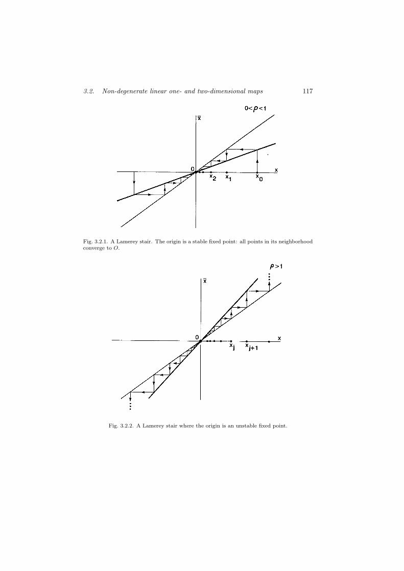
3.2. Non-degenerate linear one- and two-dimensional maps 117
Fig. 3.2.1. A Lamerey stair. The origin is a stable fixed point: all points in its neighborhoodconverge to O.
Fig. 3.2.2. A Lamerey stair where the origin is an unstable fixed point.

118 Chapter 3. Structurally Stable Periodic Trajectories
Fig. 3.2.3. An example of a Lamerey spiral; a trajectory starting from x0 looks like aclockwise-right-angled spiral.
Fig. 3.2.4. An example of an “unstable” Lamerey spiral. A trajectory xi diverges fromthe fixed point at the origin.

3.2. Non-degenerate linear one- and two-dimensional maps 119
In the degenerate case where ρ = 1, all points are fixed. When ρ = −1
all points, except for the origin O, are periodic with period equal to 2, i.e. the
fixed points of the map T 2 defined by:
¯x = x (¯x = −(x) ⇐ x = −x) .
Let us now consider a two-dimensional Poincare map(u1
u2
)
=
(
a11 a12
a21 a22
) (u1
u2
)
. (3.2.2)
When both eigenvalues of the matrix A are real and different, a non-
degenerate linear change of coordinates brings the Poincare map to the form
x = ρ1x , y = ρ2y . (3.2.3)
The iterations of an initial point (x0, y0) are given by
xj = ρj1 x0 , yj = ρj2 y0 . (3.2.4)
There are four cases to be considered:
(1) |ρi| < 1 (i = 1, 2). In this case the fixed point at the origin O is
exponentially stable and is called a stable node. Let us assume |ρ1| > |ρ2|,
then all trajectories, except for those which lie on the non-leading (strongly
stable) axis y, tend to O tangentially to the leading axis x as j → +∞. The
behavior of the trajectories in a neighborhood of a stable node is shown in
Figs. 3.2.5 and 3.2.6.
(2) |ρi| > 1 (i = 1, 2). This case is reduced to the previous one if we
consider the inverse map T−1. The fixed point is called an unstable node.
(3) |ρ1| < 1 and |ρ2| > 1. A fixed point with multipliers of this type is
called a saddle. It is seen from (3.2.4) that both x and y axes are invariant
with respect to the map (3.2.3). Points on the x-axis tend to O as j → +∞,
whereas points on the y-axis tend to O as j → −∞. For this reason, the
x-axis and the y-axis are called the stable subspace and the unstable subspace
respectively of the saddle O. All other trajectories pass close but away from
the saddle. Their loci depend upon the signs of the multipliers; four possible
variants are presented in Figs. 3.2.7a–3.2.7d.
(4) Complex-conjugate multipliers ρ1,2 = ρe±iω. In this case the Poincare
map may be written in the form
x = ρ(x cosω − y sinω) ,
y = ρ(y cosω + x sinω) ,

120 Chapter 3. Structurally Stable Periodic Trajectories
12
Fig. 3.2.5. A stable node (+) with positive multipliers 0 < ρ2 < ρ1 < 1. A trajectory T iMof the point M enters the origin tangentially to the leading direction x.
121 2
Fig. 3.2.6. A stable node “−” with the negative leading multiplier ρ1; therefore, the x-coordinate changes its sign after each iteration.

3.2. Non-degenerate linear one- and two-dimensional maps 121
(a)
Fig. 3.2.7(a). A saddle (+,+). The y-axis coincides with the unstable direction, the x-axiswith the stable one.
(b)
Fig. 3.2.7(b). A saddle (+,−). The sign of the y-coordinate of the trajectory T iM changesafter each iteration.

122 Chapter 3. Structurally Stable Periodic Trajectories
(c)
Fig. 3.2.7(c). A saddle (−, +). The “jumping” direction is here the x-axis because thecorresponding multiplier ρ1 is negative.
(d)
Fig. 3.2.7(d). A saddle (−,−). The trajectory of the initial point M runs away from theorigin along the hyperbolas located in 1st and 3rd quadrants.

3.2. Non-degenerate linear one- and two-dimensional maps 123
Fig. 3.2.8. A stable focus.
or in polar coordinates (r, ϕ), in the form
r = ρ r ,
ϕ = ϕ+ ω .(3.2.5)
The j-th iteration of the point (r0, ϕ0) is given by
rj = ρj r0 ,
ϕj = ϕ0 + ω j .
When ρ < 1, the point O is called a stable focus. In this case, all trajectories
lie on logarithmic spirals winding into the origin as shown in Fig. 3.2.8.
When ρ > 1, the fixed point O is called an unstable focus. In this case, all
trajectories diverge from any neighborhood of the point O as j → +∞.
In the degenerate case where ρ = 1, we note from (3.2.5) that r = r, i.e. any
circle with center at the origin O is invariant with respect to the map. In its
restriction to an invariant circle, the map has the form
ϕ = ϕ+ ω (mod 2π) .

124 Chapter 3. Structurally Stable Periodic Trajectories
Fig. 3.2.9. An example of the behavior of the trajectories of a degenerate map. The entirex-axis consists of fixed points.
If ω is commensurable with 2π, i.e. ω = 2πM/N for some integers M and N ,
then all points are periodic with period N as
ϕN = ϕ+N ω = ϕ+ 2πM = ϕ (mod 2π) .
Thus, all points are the fixed point of the N -th iterate of the map T . This
implies that TN is the identity map.
If ω is not commensurable with 2π, then the trajectory of any point ϕ0 is
non-periodic. Moreover, one can show that the set of the points
ϕjj=+∞j=−∞
is dense on any circle.
Figure 3.2.9 illustrates one more degenerate case: ρ1 = 1, |ρ2| < 1. Here,
all points on the x-axis are fixed points. Any straight-line x = constant is
invariant with respect to the map. The trajectories on each straight-line tend
to the corresponding fixed point.

3.3. Fixed points of high-dimensional linear maps 125
3.3. Fixed points of high-dimensional linear maps
Let us consider an n-dimensional map
x = Ax , A ∈ Rn . (3.3.1)
As in our previous discussion of linear systems of differential equations, let us
choose the coordinates such that the matrix A is represented in the real Jordan
form:
A = A0 + ∆A , (3.3.2)
where A0 is the block-diagonal matrix
A0 =
A1 0A2
. . .
0 An
. (3.3.3)
The block
Ai = (ρ) , (3.3.4)
corresponds to each real eigenvalue (multiplier) ρ of the matrix A. The block
Ai = ρ
(cosω − sinωsinω cosω
)
(3.3.5)
corresponds to each pair of complex-conjugate multipliers ρe±iω. The matrix
∆A is non-zero only when the matrix A has multiple eigenvalues. In this case
a basis may be chosen in Rn such that
‖∆A‖ ≤ ε (3.3.6)
for an infinitesimally small constant ε > 0 (see Sec. 2.3).
It is evident that
‖A0‖ ≤ ρ′ ,
where ρ′ is the maximum of the absolute values of all eigenvalues of the matrix
A. Therefore
‖A‖ ≤ ρ′ + ε . (3.3.7)
A trajectory of map (3.3.1) is given by the equation
xj = Aj x0 . (3.3.8)

126 Chapter 3. Structurally Stable Periodic Trajectories
When all eigenvalues of the matrix A lie strictly inside the unit circle, it follows
from (3.3.7) that
‖xj‖ ≤ ‖A‖j‖x0‖ ≤ (ρ′ + ε)j ‖x0‖ for j ≥ 0 , (3.3.9)
i.e. all trajectories converge exponentially to the fixed point at the origin as
j → +∞.
A transition to an arbitrary basis alters the estimate (3.3.9) so that some
constant, generally speaking greater than 1 (see formulas (2.3.17) and (2.3.18)
in Sec. 2.3), appears in the right-hand side.
As in the case of a stable equilibrium state, we may introduce the notions
of leading and non-leading multipliers of a stable fixed point.
Let us arrange the multipliers in order of decreasing absolute value, and let
the first m multipliers be of equal absolute value, i.e.
|ρ1| = · · · = |ρm| = ρ′ , |ρi| < ρ′ < 1 for i ≥ m+ 1 .
Denote by EL the m-dimensional eigen-subspace of the matrix A which
corresponds to multipliers (ρ1, . . . , ρm), and by Ess the (n − m)-dimensional
eigen-subspace which corresponds to multipliers (ρm+1, . . . , ρn). The subspace
EL is called the leading invariant subspace and Ess is called the non-leading,
or strongly stable, invariant subspace.
Each vector x ∈ Rn is uniquely represented in the form
x = u+ v ,
where u ∈ EL and v ∈ Ess. In coordinate system (u, v) the map (3.3.1) may
be written as follows
u = ALu ,
v = Assv ,
where spectr AL = ρ1, . . . , ρm and spectr Ass = ρm+1, . . . , ρn. A trajec-
tory of the map is given by the formula
uj = AjLu0 ,
vj = Ajssv0 .(3.3.10)
As in (3.3.7) we have
‖uj‖ ≥ (ρ′ − ε)j ‖u0‖ ,
‖vj‖ ≤ (|ρm+1| + ε)j ‖v0‖ ,(3.3.11)

3.3. Fixed points of high-dimensional linear maps 127
where ε can be made arbitrarily small by an appropriate choice of bases for
EL and Ess. Hence we obtain the following inequality
‖vj‖ · ‖u0‖ν ≤ ‖v0‖ · ‖uj‖
ν , (3.3.12)
for some constant ν > 1.
Thus, all trajectories for which u0 6= 0 (i.e. outside of Ess) tend to O
tangentially to the subspace EL as j → +∞. Moreover, any such trajectory
converges to O not faster than (ρ′−ε)j , whereas the trajectories in Ess converge
to O faster than (|ρm+1| + ε)j , where the constant ε > 0 may be chosen
arbitrarily small.
As regards the behavior of trajectories in the leading coordinates u we can
point out three major classes of stable fixed points:
(1) In the case m = 1, i.e. when ρ1 is real and |ρi| < ρ1 (i = 2, . . . , n), the
leading subspace is a straight line. When ρ1 > 0 all trajectories outside
of Ess converge to O along a certain direction, either from u > 0 or from
u < 0, as shown in Fig. 3.2.5. Such a fixed point is called a stable node
(+).
(2) When m = 1 and ρ1 < 0 all trajectories except those in Ess converge
to O along the u-axis but after each successive iteration the sign of the
u-coordinate changes as shown in Fig. 3.2.6. Such a fixed point is called
a stable node (−).
(3) When m = 2 and ρ1,2 = ρ′ e±iω, ω /∈ 0, π, the fixed point is called a
stable focus. The leading subspace of the fixed point is two-dimensional
and all trajectories outside of Ess approach O along spirals tangential to
the plane u.
The case of a completely unstable fixed point where the absolute values of
all of its multipliers ρi are greater than 1, is reduced to the previous case via
its inverse map (as the eigenvalues of the matrix A−1 are equal exactly to ρ−1i ).
Therefore, an estimate
‖xj‖ ≤ ‖A−1‖j‖x0‖ ≤ (ρ′ − ε)j ‖x0‖ for j ≤ 0 , (3.3.13)
analogous to (3.3.9), is valid, where ρ′ is the smallest absolute value of the
multipliers ρi, (i = 1, . . . , n). All trajectories tend exponentially to O as
j → −∞.

128 Chapter 3. Structurally Stable Periodic Trajectories
As in the case of stable fixed points, we may now define leading and non-
leading invariant subspaces and select three principal classes of completely
unstable fixed points: an unstable node (+), an unstable node (−) and an
unstable focus according to the signs of the multipliers.
When some multipliers of the fixed point lie strictly inside the unit cycle
|ρi| < 1 (i = 1, . . . , k) and all others lie outside of it: |ρj | > 1 (j = k+1, . . . , n),
the fixed point is called a saddle fixed point. A linear non-degenerate change
of coordinates transforms the map into the form
u = A−u ,
v = A+v ,(3.3.14)
where spectr A− = ρ1, . . . , ρk, spectr A+ = ρk+1, . . . , ρn, u ∈ Rk, v ∈
Rn−k. For u and v we have estimates analogous to (3.3.9) and (3.3.13), re-
spectively. This means that the trajectories from the stable invariant subspace
Es : v = 0 and the unstable invariant subspace Eu : u = 0 tend exponentially
to the saddle point O as j → +∞ and j → −∞, respectively. All other
trajectories escape from a small neighborhood of O.
Thus, in the stable subspace Es the saddle is a stable fixed point and in the
unstable subspace Eu it is a completely unstable fixed point. Furthermore, in
Es and Eu we may select stable and unstable leading and non-leading manifolds
EsL, EuL, Ess and Euu. We will call the direct sum EsE = Es⊕EuL the extended
stable invariant subspace and EuE = Eu ⊕ EsL the extended unstable invariant
subspace. The invariant subspace EL = EuE ∩ EsE is called the leading saddle
invariant subspace.
When the point O is a node in both Es and Eu, O is called a saddle. When
O is a focus in at least one of the subspaces Es or Eu, it is called a saddle-focus.
3.4. Topological classification of fixed points
We saw in Chap. 2 that near a structurally stable equilibrium state a system of
differential equations is topologically equivalent to its linearization. A similar
statement pertains to structurally stable fixed points. This allows us to present
a complete classification of systems of differential equations near a structurally
stable periodic trajectory.
In this context an appropriate analog of topological equivalence is the no-
tion of topological conjugacy.

3.4. Topological classification of fixed points 129
Definition 3.1. Two diffeomorphisms T1 and T2 defined in regions D1 and
D2, respectively, are said to be topologically conjugate in the regions U1 ⊆ D1
and U2 ⊆ D2 if there exists a homeomorphism η : U1 → U2 which transforms
trajectories (semi-trajectories, intervals of trajectories) of the first diffeomor-
phism onto trajectories (semi-trajectories, intervals of trajectories) of the sec-
ond diffeomorphism.
In other words, for any point x ∈ D1 the following equality holds (see
Fig. 3.4.1).
η(T1(x)) = T2(η(x)) . (3.4.1)
Theorem 3.1. (Grobman Hartman) Let O be a structurally stable fixed
point of a diffeomorphism T. Then there exist neighborhoods U1 and U2 of
the point O where the diffeomorphism T and its linear part are topologically
conjugate.
In the structurally unstable (non-rough) case an analogous statement does
not hold. It is easy to show that when the matrix A of a linear map
x = Ax (3.4.2)
Fig. 3.4.1. Graphical representation of the homeomorphism η(T1(x)) = T2(η(x)) realizingthe topological conjugacy between two maps T1 and T2 defined in subregions U1 and U2,respectively.

130 Chapter 3. Structurally Stable Periodic Trajectories
has some multipliers equal to 1 in absolute value, then one can add a nonlinear
term g(x) such that the map
x = Ax+ g(x) (3.4.3)
is not topologically conjugate to its linear part (3.4.2). For example, the one-
dimensional map
x = x+ x2
has only one fixed point O (see Fig. 3.4.2), whereas all points on the bisectrix
are fixed points of the associated linearized map
x = x .
Consider another example: the map
x = −x+ x3 ,
Fig. 3.4.2. A Lamerey stair. The graph of the function f(x) = x + x2 is tangent to thebisectrix at the fixed point of the saddle-node type.

3.4. Topological classification of fixed points 131
Fig. 3.4.3. A Lamerey spiral of the map x = −x + x3. Outside of the origin the derivativeof the map is less than 1 in absolute value: the fixed point is stable.
possessing the stable fixed pointO (see Fig. 3.4.3) is not topologically conjugate
to its linear part
x = −x ,
for which all points (apart from O) are periodic trajectories of period 2.
For our next example let us examine a linear map possessing a fixed point
with a pair of complex-conjugate multipliers e±iω
x = x cosω − y sinω ,
y = x sinω + y cosω .(3.4.4)
All trajectories lie on invariant circles centered at the point O(0, 0) (see
Sec. 3.2). This map is not conjugate to the map
x = x cosω − y sinω − x(x2 + y2) cosω ,
y = x sinω + y cosω − y(x2 + y2) cosω(3.4.5)
whose trajectories tend to O along spirals (the analogous example of an equi-
librium state is given in Sec. 2.5).

132 Chapter 3. Structurally Stable Periodic Trajectories
It follows from Theorem 3.1 that when all multipliers of the fixed point
O of the diffeomorphism T are less than 1 in absolute value, then all forward
trajectories tend to O. When all multipliers lie outside of the unit circle,
the backward trajectory of a point from a small neighborhood of the point
O tends to the fixed point. Forward iterations of the map T force all tra-
jectories (excluding the fixed point) to escape from a neighborhood of the
fixed point.
In the saddle case where there are multipliers both inside and outside of
the unit circle, the fixed point has (locally) a stable invariant manifold W sloc
and an unstable invariant manifold W uloc which are the images of the invariant
subspaces Es and Eu of the associated linearized system by the homeomorphism
η which establishes the topological conjugacy. Therefore, the forward semi-
trajectory of any point in W sloc lies entirely in W s
loc and tends to the saddle
point O. On the other hand, given any point in W uloc its backward semi-
trajectory lies entirely in W uloc and tends to O. The dimension of the stable
manifold is equal to the number of the multipliers inside the unit circle and the
dimension of the unstable manifold is equal to the number of multipliers outside
of the unit circle. Trajectories of the points which do not lie in W sloc ∪W
uloc
diverge from any neighborhood of the saddle.
It is obvious that if one diffeomorphism near a saddle fixed point is topo-
logically conjugate to another diffeomorphism near another fixed point, then
the dimensions of the stable (unstable) manifolds of both saddle points must
be equal (for generality, in the case of a stable fixed point we can assume that
Wu = ∅ and, therefore dim W u = 0; for a completely unstable point assume
that W s = ∅ and dim W s = 0). However, in contrast to the case of struc-
turally stable equilibrium states, the dimensions of the stable and the unstable
manifolds are not the only invariants of the topological conjugacy near the
fixed points.
In order to find new invariants we notice that the Grobman–Hartman the-
orem may be generalized as follows
In a neighborhood of the origin a linear non-singular map which has no
multipliers on the unit circle, is topologically conjugate to any, suffi-
ciently close map.
This implies in particular that any two close, linear maps are topologically
conjugate. It follows that for two arbitrary matrices A0 and A1 the maps
x = A0x and x = A1x

3.4. Topological classification of fixed points 133
are topologically conjugate if we can construct a family of the matrices A(s)
depending continuously on the parameter s ∈ [0, 1] such that A(0) = A0 and
A(1) = A1, provided that all matrices A(s) are non-singular and have no
eigenvalues on the unit circle.
It is not hard to verify that such a family exists if and only if both matrices
A0 and A1 have the same number of multipliers both inside and outside of the
unit circle and the same values δs and δu, where δs = signk∏
i=1
ρi as well as
δu = signn∏
i=k+1
ρi, where (ρ1, . . . , ρk) are the multipliers inside the unit circle,
and (ρk+1, . . . , ρn) are the multipliers which lie outside of the unit circle. The
values δs and δu remain unchanged while A0 is changed continuously to A1
because the product of the multipliers can change its sign only when at least
one multiplier vanishes, which is only possible for degenerate maps.
Thus, when some fixed points have the same topological type, i.e. the same
set of four numbers (k, δs, n − k, δu), then they are topologically conjugate,
i.e. there exists a homeomorphism establishing topological conjugacy among
the diffeomorphisms defined near these fixed points. In particular, near a fixed
point any diffeomorphism is topologically conjugate to a map
x = Asx , y = Auy , (3.4.6)
where As and Au are, respectively, the (k×k)-matrix and the (n−k)×(n−k)-
matrices:
As =
1/2 01/2
. . .
0 δs/2
, Au =
2 02
. . .
0 2δu
.
We should emphasize that maps of the kind (3.4.6) with different values
of δs cannot be topologically conjugate since the restriction x = Asx of the
map (3.4.6) to the stable invariant subspace y = 0 preserves the orientation in
Rk provided that δs = 1, but does not preserve it if δs = −1. This assertion
applies to δu as well. In conclusion we come to the following theorem.
Theorem 3.2. Two structurally stable fixed points are topologically conjugate
if and only if they are of the same topological type.

134 Chapter 3. Structurally Stable Periodic Trajectories
Thus, the number of topological types of structurally stable fixed points
of n-dimensional maps exceeds the number of topological types of structurally
stable equilibrium states of differential equations in Rn. So, a two-dimensional
diffeomorphism may have two types of stable and unstable fixed points and
four types of saddle fixed points. For example, the two linear maps
x = x/2
y = y/2and
x = x/2
y = −y/2
have the fixed points of node type but the first point is orientable whereas the
second is non-orientable.
(Note: a fixed point possessing a pair of complex-conjugate multipliers has
also the topological type of orientable node.)
Observe next that the maps
x = 2x
y = 2yand
x = 2x
y = −2y
have, respectively, an orientable and a non-orientable unstable topological node
at the origin.
Examples of topological saddles (δs = (+), δu = (+)) and (δs = (−), δu =
(−)) are given, respectively, by:
x = x/2
y = 2yand
x = −x/2
y = −2y
Examples of topological saddles (+,−) and (−,+) are given, respectively,
by
x = x/2
y = −2yand
x = −x/2
y = 2y
It is clear that in the case δs > 0 the stable invariant manifold (here, the
x-axis) of the saddle point is subdivided by the point O into the two parts,
namely, the rays x > 0 and x < 0, each of which is invariant with respect to
the map. In the case δs < 0 these rays are no longer separately invariant in
the sense that the map takes one onto the other. Analogously, the value δudetermines the structure of the unstable manifold of the saddle point O.
We must emphasize that the Poincare map always preserves orientation
in Rn, i.e. the product of all multipliers of a periodic trajectory is positive.

3.5. Properties of nonlinear maps near a stable fixed point 135
This implies that the values δs and δu of the fixed point of the Poincare map
must have the same sign. Nevertheless, restricted to an invariant (stable or
unstable) manifold, the Poincare map may not continue to preserve orientation
(for example, when both δs and δu are negative). Thus, the study of fixed
points of non-orientable maps makes the sense.
We showed in Sec. 3.1 that the values of the multipliers of a fixed point of the
Poincare map (and, consequently, its topological type) are independent of the
choice of the cross-section, i.e. we can always correctly define the topological
type (k, δs, n − k, δu) of a periodic trajectory. In order to complete our
classification we refer to the following simple statement.
Lemma 3.1. Let a system X1 of differential equations have a periodic trajec-
tory L1 and a system X2 have a periodic trajectory L2. Then, the system X1
in a neighborhood of the trajectory L1 is topologically equivalent to the system
X2 in a neighborhood of the trajectory L2 if and only if the respective Poincare
maps are topologically conjugate near the corresponding fixed points (regardless
of the choice of cross-sections)
From this lemma and from Theorem 3.2 we have the following theorem.
Theorem 3.3. Two structurally stable periodic trajectories are locally topo-
logically equivalent if and only if they have the same topological type.
3.5. Properties of nonlinear maps near a stable fixedpoint
In the previous section we formally have presented a complete description of
dynamical systems near a structurally stable periodic trajectory. However,
such a topological classification of periodic trajectories, as well as equilibrium
states, is too crude. For example, the assertion concerning the equivalence of a
node and a focus seems to be rather strange from a practical point of view. We
will consider below more subtle (and more significant) features of structurally
stable fixed points.
Suppose the map
x = Ax+ h(x) , (3.5.1)
where
h(0) = 0 , h′(0) = 0 , (3.5.2)

136 Chapter 3. Structurally Stable Periodic Trajectories
has a stable fixed point at the origin. This means that the absolute values of
all multipliers ρi (i = 1, . . . , n) of the matrix A are strictly less than 1. It is
not hard to verify that all trajectories beginning from a small neighborhood of
the origin tend exponentially to O. Indeed, if we choose the Jordan basis, we
can verify that the estimate (3.3.9) for the norm of the matrix A is fulfilled;
namely,
‖A‖ ≤ ρ′ + ε ,
where ρ′ = maxi=1,...,n
|ρi| < 1. From the relation
h(x) = h(0) + x
∫ 1
0
h′(sx)ds
we have
‖h(x)‖ ≤ ‖x‖ max‖y‖≤‖x‖
‖h′(y)‖ .
Hence
‖h(x)‖ ≤ ε‖x‖ , (3.5.3)
where ε > 0 can be chosen arbitrarily small since x is assumed to be small.
Consequently, for map (3.5.1) we obtain
‖x‖ ≤ ‖A‖ ‖x‖ + ‖h(x)‖ ≤ (ρ′ + 2ε)‖x‖ ,
or, equivalently for the j-th iteration of an initial point x0
‖xj‖ ≤ (ρ′ + 2ε)j‖x0‖ (3.5.4)
where xj → 0 as j → +∞ since ρ′ < 1 and since ε can be made arbitrarily
small.
Let us now reorder the eigenvalues of the matrix A so that
|ρ1| = · · · = |ρm| = ρ′ , |ρi| < ρ′ for i = m+ 1, . . . , n .
The matrix A can be then represented in the form
A =
(
A1 0
0 A2
)
,
where spectrA1 = ρ1, . . . , ρm and spectrA2 = ρm+1, . . . , ρn. The map
(3.5.1) now takes the form
u = A1u+ f(u, v) ,
v = A2v + g(u, v) ,(3.5.5)
3.5. Properties of nonlinear maps near a stable fixed point 137
where u = (u1, . . . , um) and v = (v1, . . . , vn−m) are the projections of x onto
the leading and the non-leading subspaces of the matrix A, the functions f ,
g ∈ Cr, and
f(0) = 0 , g(0) = 0 , f ′(0) = 0 , g′(0) = 0 . (3.5.6)
In Chap. 5 we will prove the following theorem
Theorem 3.4. (On the non-leading manifold) In a neighborhood U of
the point O there exists a unique (n−m)-dimensional Cr-smooth non-leading
(strongly stable) invariant manifold W ssloc of the form
u = ϕ(v)
where
ϕ(0) = ϕ′v(0) = 0 . (3.5.7)
The following result follows from Theorem 3.4.
Theorem 3.5. For any point x0 that does not lie in W ssloc the associated tra-
jectory xjj≥0 tends to O along the leading direction v = 0, and
‖xj‖ ≥ C (ρ′ − ε)j dist (x0, Wssloc) , (3.5.8)
where C is some positive constant and ε can be made arbitrarily small by
choosing suitably small x0.
Proof. Firstly, let us straighten the manifold W ssloc by the following change
of variables
w = u− ϕ(v) . (3.5.9)
In the new variables the equation of W ssloc is w = 0. The invariance of the
manifold implies that w = 0 when w = 0. Since the function ϕ(v) contains
no linear terms (see (3.5.7)), the transformation (3.5.9) does not change the
linear part of the map. As a result, in the new variables map (3.5.5) becomes
w = (A1 + f(w, v)) w (3.5.10)
v = A2v + g(w + ϕ(v), v) , (3.5.11)
where
f(0, 0) = 0 . (3.5.12)

138 Chapter 3. Structurally Stable Periodic Trajectories
In the Jordan basis (see Sec. 3.3), we have for the norm of the matrix A1
‖A−11 ‖−1 ≥ ρ′ − ε/2 .
By (3.5.10) and (3.5.12) this implies that
‖w‖ ≥ (ρ′ − ε) ‖w‖ (3.5.13)
provided that ‖w, v‖ is sufficiently small. As we have shown already, when
the norm of the initial point ‖w0, v0‖ is sufficiently small, the norm ‖wj , vj‖
is also small for all j ≥ 0. Therefore, inequality (3.5.13) is valid for any pair
(wj , wj+1 = wj). Hence, we obtain the estimate
‖wj‖ ≥ (ρ′ − ε)j‖w0‖
i.e. the inequality (3.5.8) is proven.
Let us now verify that when an initial point does not belong to W ssloc, its
trajectory tends to O along the leading subspace v = 0. When w 6= 0 let
us consider the value z = ‖v‖/‖w‖. We seek to show that zj → 0 along the
trajectories (wj , vj)j≥0 of the map (3.5.10)–(3.5.11).
For ‖w‖ we have the estimate (3.5.13). Similarly, from (3.5.11) one obtains
‖v‖ ≤ (|ρm+1| + ε) ‖v‖ + ‖w‖ max ‖f ′u‖ ,
where the maximum is taken over a neighborhood of O of diameter equal to
‖w, v‖. By (3.5.13), it follows that
zj+1 ≤ (|ρm+1| + ε)‖vj‖/(ρ′ − ε)‖wj‖
+max ‖f ′u‖/(ρ
′ − ε) ≡ µzj + κj , (3.5.14)
where µ = (|ρm+1| + ε)/(ρ′ − ε) < 1 and
κj → 0 as j → +∞ . (3.5.15)
From (3.5.14) we obtain
µ−(j+1)zj+1 ≤ µ−jzj + µ−(j+1)κj ,
µ−(j+1)zj+1 ≤ z0 +
j∑
i=0
µ−(i+1)κi ,
zj ≤ z0µj +
j−1∑
i=0
µj−(i+1)κi .

3.5. Properties of nonlinear maps near a stable fixed point 139
Since µ < 1, the first summand decays to zero as j → ∞. Hence, in order
to prove that zj → 0 we need to show that the sum
Ij =
j−1∑
i=0
µj−(i+1)κi → 0 .
This expression readily holds if we let κj → 0. Let us choose a natural number
J and break the sum into two parts:
Ij =J−1∑
i=0
µj−(i+1)κi +
j−1∑
i=J
µj−(i+1)κi .
Observe that
Ij ≤ µj−JJ−1∑
i=0
κi +
(j−1∑
i=J
µj−(i+1)
)
maxi≤J
κi
≤ µj−JJ−1∑
i=0
κi + (1 − µ)−1 maxi≥J
κi . (3.5.16)
By virtue of (3.5.15) the second term in (3.5.16) can be made arbitrarily
small by increasing J . By choosing J sufficiently large we may make the first
term in (3.5.16) arbitrarily small too and, therefore, Ij arbitrary small if let
j → +∞.
Thus, when w0 6= 0, ‖vj‖/‖wj‖ → 0, i.e. any trajectory which does not lie
in W ssloc converges to the leading manifold as j → +∞. Thus, we have proven
Theorem 3.5
The map (3.5.10)–(3.5.11) on the non-leading manifold w = 0 is written in
the form
v = A2 v + g(ϕ(v), v) . (3.5.17)
On this manifold the point O is a stable fixed point with the multipliers
(ρm+1, . . . , ρn). The results obtained above can be applied to this mapping.
In particular, the following exponential estimate analogous to (3.5.4) holds:
‖vj‖ ≤ C (|ρm+1| + ε)j ‖v0‖ , (3.5.18)
i.e. any trajectory from W ssloc tends to O exceedingly fast. Since Theorems 3.4
and 3.5 hold for the map (3.5.17), it follows that almost all trajectories in W ssloc

140 Chapter 3. Structurally Stable Periodic Trajectories
tends to O with the exponential rate equal asymptotically |ρm+1|. Those par-
ticular trajectories which tend to O faster, form a Cr-smooth manifold W sss
loc
tangential at O to the eigen-subspace of the matrix A which corresponds to
the multipliers whose absolute values are less than |ρm+1|. For the restriction
of the map to W sssloc , the theorem on the non-leading manifold can also be ap-
plied, and so on. We again obtain a hierarchy of non-leading manifolds: W ssloc,
W sssloc , W ssss
loc , . . . , composed of trajectories with higher and higher velocities of
convergence to the fixed point.
Just like the linear case, we can select three main types of stable fixed
points which depend on the behavior of the map in the leading coordinates: a
node (+), a node (−) and a focus.
The point O is called a node when m = 1, i.e. when the leading multiplier
ρ1 is unique and real:
1 > |ρ1| > |ρi| (i = 2, . . . , n) . (3.5.19)
Moreover, the point is called a node (+) when 0 < ρ1 < 1, and it is called a
node (−) when −1 < ρ1 < 0.
The point O is called a focus when m = 2 and the leading multipliers are
complex:
1 > |ρ1| = |ρ2| > |ρi| (i = 3, . . . , n) . (3.5.20)
In the case of the node, the (n− 1)-dimensional non-leading manifold par-
titions a neighborhood of the fixed point O into two parts, namely, w > 0 and
w < 0. Here, Eq. (3.5.10) for the leading coordinate w can be written in the
form
w = ρ1w + o(w) . (3.5.21)
One can see that when ρ1 > 0 each part is invariant with respect to the
map. The trajectories which do not lie in W ssloc tend monotonically to O strictly
along one of two directions, either from the region w > 0, or from the opposite
side w < 0.
When ρ1 < 0 the parts cycle under the action of the map, i.e. the sign of
the leading coordinate changes with every iteration.
In the case of the focus, the non-leading manifold is (n − 2)-dimensional
and it no longer partitions a neighborhood of the point O. Having introduced
ρ1,2 = ρe±iω, Eq. (3.5.10) for the leading coordinates becomes
w1 = ρ(cosω + · · · ) w1 − ρ(sinω + · · · ) w2 ,
w2 = ρ(sinω + · · · ) w1 + ρ(cosω + · · · ) w2 ,(3.5.22)

3.6. Saddle fixed points. Invariant manifolds 141
or in polar coordinates
r = (ρ+ · · · ) r (3.5.23)
ϕ = ϕ+ ω + · · · , (3.5.24)
where the ellipsis denotes the terms of a higher order. It follows from (3.5.23)
and (3.5.24) that all trajectories which do not belong to W ssloc must spiral
towards to O (tangentially to the leading plane v = 0).
The case where |ρi| > 1, (i = 1, . . . , n) is reduced to that discussed above
by considering the inverse map. In this case a trajectory is estimated by
‖xj‖ ≤
(
mini=1,...,n
ρi − 2ε
)j
‖x0‖ for j ≤ 0 . (3.5.25)
The associated fixed point is exponentially completely unstable. The exis-
tence of the smooth non-leading manifold W uuloc can be established in the same
way as for W ssloc of the stable fixed point but assuming on this occasion that
j → −∞. Depending on the behavior of the trajectories in the leading coordi-
nates there exist fixed points of the following types: node (+), node (−) and a
focus.
We conclude this section with a theorem on the leading invariant manifold
(see its proof in Chap. 5.)
Theorem 3.6. (On the leading invariant manifold) A stable fixed point O
has an m-dimensional Cmin(r,rL)-smooth invariant manifold WL
loc (not unique
in general) which is tangent at the point O to the subspace v = 0; here
rL =
[ln ρm+1
ln ρ1
]
≥ 1 , (3.5.26)
where [x] denotes the largest integer strictly less than x, and m is the number
of the leading multipliers.
3.6. Saddle fixed points. Invariant manifolds
Let us consider next a map T possessing a structurally stable fixed point O
of saddle type whose first k multipliers lie inside the unit circle and whose
remaining (n − k) multipliers lie outside of the unit circle, i.e. |ρi| < 1 (i =
1, . . . , k), |ρj | > 1, (j = k + 1, . . . , n), where k 6= 0, n. For convenience, let us

142 Chapter 3. Structurally Stable Periodic Trajectories
denote the multipliers inside the unit circle by (λ1, . . . , λk), and those outside
by (γ1, . . . , γn−k). We will also assume that the multipliers are ordered in the
following manner
|λk| ≤ · · · ≤ |λ2| ≤ |λ1| < 1 < |γ1| ≤ |γ2| ≤ · · · ≤ |γn−k| .
A linear non-degenerate change of variables near the point O transforms the
map T to the form
u = A−u+ f(u, v) ,
v = A+v + g(u, v) ,(3.6.1)
where u ∈ Rk and v ∈ R
n−k, Spectrum A− = λ1, . . . , λk and Spectrum
A+ = γ1, . . . , γn−k; f, g are Cr-smooth (r ≥ 1) functions which vanish at
the origin along with their first derivatives.
The study of the map T near a saddle fixed point resembles that of a system
of differential equations near a saddle equilibrium point. It can be reduced to
the problem of the existence of a stable and an unstable invariant manifolds
of the point O. We examine this problem in detail below. Poincare proved
the existence of analytical invariant manifolds for analytical maps. Later, the
smooth case was considered by Hadamard [31] who proved the existence of
invariant manifolds satisfying a Lipschitz condition.
Theorem 3.7. (Hadamard’s theorem) The saddle fixed point O has two
invariant manifolds: a stable manifold W sloc : v = ψ∗(u) and an unstable man-
ifold Wuloc : u = ϕ∗(v), where ψ∗(u) and ϕ∗(v) satisfy the following Lipschitz
conditions:
‖ψ∗(u2) − ψ∗(u1)‖ ≤ N‖u2 − u1‖ , (3.6.2)
‖ϕ∗(v2) − ϕ∗(v1)‖ ≤ L‖v2 − v1‖ , (3.6.3)
for some constants N > 0 and L > 0.
Proof. We prove only the existence of W uloc as the inverse map T−1 can also
be represented in the form (3.6.1) with the only difference that the variables u
and v exchange roles. Therefore, having proven that the map T has an invariant
manifold W uloc of the form u = ϕ∗(v), by repeating the same arguments for the
map T−1 we can prove that there exists an invariant manifold of the form
v = ψ∗(u), i.e. the desired manifold W sloc.

3.6. Saddle fixed points. Invariant manifolds 143
Let us select a small δ > 0 and surround the point O by a neighborhood
D1 ⊗D2 in Rn, where D1 and D2 are spheres of diameter equal to δ in R
k and
Rn−k, respectively. Choose an arbitrary surface W of the form u = ϕ(v) such
that
‖ϕ‖ ≤ δ (3.6.4)
‖ϕ′‖ ≤ L (3.6.5)
for some L > 0. We will show below that when δ is sufficiently small then
the intersection T (W) ∩ (D1 ⊗ D2) is a surface of the same form u = ϕ(v)
where ϕ satisfies conditions (3.6.4)–(3.6.5) with the same constant L. This
allows us to consider a sequence of surfaces Wj : u = ϕj(v)j=∞j=0 which are
the sequential images of the initial surface W under the map T : ϕj = T jϕ.
We will show further that this sequence converges uniformly to some surface
u = ϕ∗(v) satisfying a Lipschitz condition. Moreover ϕ∗ does not depend on
the initial function ϕ. By construction, ϕ∗ = ϕ∗, i.e. its graph is invariant with
respect to the map T . Thus, the surface u = ϕ∗(v) is the desired invariant
manifold W uloc: T (Wu
loc) ∩ (D1 ⊗D2) = Wuloc.
Step 1. Let us choose an arbitrary surface W of the form u = ϕ(v) which
satisfies conditions (3.6.4) and (3.6.5) for some L. By substituting u = ϕ(v)
into (3.6.1) we obtain a parametric representation
u = A− ϕ(v) + f(ϕ(v), v) , (3.6.6)
v = A+ v + g(ϕ(v), v) , (3.6.7)
for the image of the surface W under the map T , where v can take arbitrary
values in D2.
Let us now show that for any v whose norm does not exceed δ the value u
is uniquely defined by (3.6.6) and (3.6.7). To do this we rewrite (3.6.7) in the
form
v = (A+)−1(v − g(ϕ(v), v)) . (3.6.8)
When δ is sufficiently small the norm ‖∂(g, f)/∂(u, v)‖ is also small. It follows
that2 ∥∥∥∥
dg(ϕ(v), v)
dv
∥∥∥∥≤ ‖g′u‖ · ‖ϕ
′‖ + ‖g′v‖
2Here ‖ · ‖ = sup ‖ · ‖.

144 Chapter 3. Structurally Stable Periodic Trajectories
is small and, therefore, by virtue of the implicit function theorem, v is uniquely
expressed in terms of v from (3.6.8). It should also be noted that ‖v‖ also does
not exceed δ. Indeed, it follows from (3.6.8) that
‖v‖ ≤ ‖(A+)−1‖(‖v‖ + ‖g′u‖ · ‖ϕ(v)‖ + ‖g′v‖‖v‖
)
whence
‖v‖ ≤ ‖(A+)−1‖(‖v‖ + ‖g′u‖ · ‖ϕ(v)‖)
1 − ‖(A+)−1‖ ‖g′v‖.
Thus, if ‖v‖ ≤ δ, then ‖v‖ ≤ δ because ‖(A+)−1‖ < 1, ‖ϕ(v)‖ ≤ δ and
‖g′(u,v)‖ is small.
So, by expressing v in terms of v from (3.6.8) and by substituting the
resulting expression into (3.6.6), we determine that for each v such that ‖v‖ ≤
δ, there exists a uniquely defined u such that the point (u, v) is the image of
some point (u, v) ∈ W. Let us denote this u by u = ϕ(v).
Step 2. Let us show that the surface TW: u = ϕ(v) satisfies conditions
(3.6.4) and (3.6.5). In other words we will show that TW lies entirely in the
δ-neighborhood (D1 ⊗D2) of the point O, and that the norm of the derivative
of the function ϕ does not exceed L. It follows from (3.6.4) and (3.6.6) that
‖u‖ ≤ ‖A−‖ ‖ϕ(v)‖ + ‖f ′u‖ · ‖ϕ(v)‖ + ‖f ′
v‖ · ‖u‖
≤ (‖A−‖ + ‖f ′u‖ + ‖f ′v‖) δ .
It follows that
‖ϕ(v)‖ ≡ ‖u‖ ≤ δ
as ‖A−‖ < 1 and the norm ‖f ′(u,v)‖ is small; i.e. condition (3.6.4) holds for ϕ
indeed.
Furthermore, from (3.6.6) and (3.6.7) we have
du
dv= A−ϕ′ + f ′u(ϕ(v), v)ϕ′ + f ′v(ϕ(v), v) ,
dv
dv= A+ + g′u(ϕ(v), v)ϕ′ + g′v(ϕ(v), v)
whence
ϕ′(v) ≡du
dv= (A−ϕ′ + f ′u(ϕ(v), v)ϕ′ + f ′v(ϕ(v), v))·
· [A+ + g′u(ϕ(v), v)ϕ′ + g′v(ϕ(v), v)]−1 .
3.6. Saddle fixed points. Invariant manifolds 145
Finally
ϕ′(v) = A−ϕ′(v)(A+)−1 + · · · ,
where the ellipsis denotes the terms of order ‖(f, g)′(u,v)‖ which tend to zero
as δ → 0. It is easy to see that since ‖A−‖ < 1 and ‖(A+)−1‖ < 1, then
‖ϕ′‖ ≤ L provided ‖ϕ′‖ ≤ L and δ is sufficiently small.
Step 3. We have shown that the map T takes any surface W satisfying
conditions (3.6.4) and (3.6.5), onto a surface satisfying the same conditions.
Hence, all iterations of the surface W are defined under the action of the map T .
Let us now show that the sequence of these iterations Wj : u = ϕj(v) converges
uniformly to some surface W∗ : u = ϕ∗(v). Since Wj+1 = T (Wj) ∩ (D1 ⊗D2),
it follows from continuity that W∗ = T (W∗) ∩ (D1 ⊗D2), i.e. this surface is
invariant with respect to the map T .
In order to prove this, we will show that there exists K < 1 such that
supv∈D2
‖ϕj+2(v) − ϕj+1(v)‖ ≤ K supv∈D2
‖ϕj+1(v) − ϕj(v)‖ . (3.6.9)
Let us choose any v ∈ D2 and consider a pair of points M1(ϕj+1(v), v) and
M2(ϕj+2(v), v). By construction, each point Mi has a pre-imageMi on the sur-
face u = ϕj+i−1(v). Assume M1(u1 = ϕj(v1), v1) and M2(u2 = ϕj+1(v2), v2).
Because M1 = TM1 and M2 = TM2, we have from (3.6.1)
u1 = A−u1 + f(u1, v1) , u2 = A−u2 + f(u2, v2) ,
v = A+v1 + g(u1, v1) , v = A+v2 + g(u2, v2) .
Hence it follows that
‖u2 − u1‖ ≤ (‖(A−‖ + ‖f ′u‖) ‖u2 − u1‖ + ‖f ′v‖ ‖v2 − v1‖ (3.6.10)
and
‖v2 − v1‖ ≤ ‖(A+)−1‖(‖g′u‖ ‖u2 − u1‖ + ‖g′v‖ ‖v2 − v1‖)
whence
‖v2 − v1‖ ≤‖(A+)−1‖ ‖g′u‖‖u2 − u1‖
1 − ‖(A+)−1‖ ‖g′v‖. (3.6.11)
For ‖u2 − u1‖ = ‖ϕj+1(v2) − ϕj(v1)‖ we have the following estimate
‖ϕj+1(v2) − ϕj(v1)‖ ≤ ‖ϕj+1(v2) − ϕj+1(v1)‖ + ‖ϕj+1(v1) − ϕj(v1)‖ .

146 Chapter 3. Structurally Stable Periodic Trajectories
The first term in this sum is estimated by
‖ϕj+1(v2) − ϕj+1(v1)‖ ≤ ‖ϕ′j+1‖‖v2 − v1‖ ≤ L‖v2 − v1‖
and the second by
‖ϕj+1(v1) − ϕj(v1)‖ ≤ ρ ,
where ρ = supv∈D2
‖ϕj+1(v) − ϕj(v)‖. Thus, we obtain
‖u2 − u1‖ ≤ ρ+ L‖v2 − v1‖ . (3.6.12)
It follows from (3.6.11) that
‖v2 − v1‖ ≤ρ‖(A+)−1‖ ‖g′u‖
1 − ‖(A+)−1‖(‖g′v‖ + L‖g′u‖))
which, after substitution into (3.6.10) with (3.6.12), gives
‖u2 − u1‖ ≤ ρ(‖A−‖ + · · · )
where the ellipsis denotes terms of the order ‖(f, g)′(u,v)‖. Since ‖A−‖ < 1,
we have
‖u2 − u1‖ = ‖ϕj+2(v) − ϕj+1(v)‖ ≤ K sup ‖ϕj+1(v) − ϕj(v)‖
for some K < 1 which does not depend on v (provided that ‖v‖ ≤ δ). If we
take the supremum in the left-hand side of this inequality with respect to all
v, then we obtain the desired inequality (3.6.9).
From (3.6.9) we obtain
‖ϕj+2(v) − ϕj+1(v)‖ ≤ Kj sup ‖ϕ2(v) − ϕ1(v)‖ ,
i.e. the series∞∑
j=1
(ϕj+1(v) − ϕj(v))
is majorized by a geometrical progression with the coefficient K < 1, and,
therefore, converges uniformly. Since the partial sums of this series are (ϕj+1(v)
− ϕ1(v)), its uniform convergence implies the uniform convergence of the se-
quence ϕj to some limit function ϕ∗.
Step 4. Let us denote the graph u = ϕ∗(v) of the function ϕ∗ by Wuloc.
By construction, this graph is invariant with respect to the map T . Note that

3.6. Saddle fixed points. Invariant manifolds 147
as ϕ∗(v) is the uniform limit of a sequence of continuous functions, it is also
continuous. Generally speaking, the smoothness of the function ϕ∗ does not
follow from our arguments (a limit of a series of smooth functions may be
non-smooth). Nevertheless, we remark that the derivatives of all functions ϕjare bounded by the same constant L:
‖ϕ′j(v)‖ ≤ L .
It follows from the inequality
‖ϕj(v1) − ϕj(v2)‖ ≤ ‖ϕ′j‖‖v1 − v2‖
that all functions ϕj satisfy a Lipschitz condition
‖ϕj(v1) − ϕj(v2)‖ ≤ L‖v1 − v2‖
for any (v1, v2) in D2. If we take a limit of this inequality as j → ∞, we obtain
‖ϕ∗(v1) − ϕ∗(v2)‖ ≤ L‖v1 − v2‖ .
Thus, we have established the existence of the invariant manifold W uloc
satisfying a Lipschitz condition. It should be noted that one can choose the
initial surface W such that it passes through the point O. It is obvious then
that all iterations of the surface W also contain the point O, and hence, the
limit surface W uloc also contains O.
Before we prove the smoothness of the invariant manifolds, let us examine
the behavior of the map in its restriction to W uloc and W s
loc. The restriction of
the map to W sloc is given by the formula
u = A−u+ f(u, ψ∗(u)) . (3.6.13)
Hence it follows from (3.6.2) that
‖u‖ ≤ ‖A−‖ ‖u‖ + ‖f ′u‖ ‖u‖ +N ‖f ′
v‖ ‖u‖ ≤(‖A−‖ + ‖f ′u‖ +N‖f ′v‖
)‖u‖ .
Thus, since ‖A−‖ < 1 and since the norm ‖f ′u‖ is small, the iterations of any
point on W sloc converge exponentially to the point O under the action of the
map T .
By the symmetry, an analogous result may be obtained for the map (3.6.1)
in its restriction to W uloc:
v = A+v + g(ϕ∗(v), v) , (3.6.14)

148 Chapter 3. Structurally Stable Periodic Trajectories
namely, for any point v on W uloc there exists a uniquely defined image v = T−1v
which iterations under the map T−1 tend uniformly and exponentially to the
point O.
Theorem 3.8. The invariant manifolds W sloc and Wu
loc belong to the Cr-class
of smoothness and at the point O they are tangent respectively to the stable
eigen-subspace v = 0 and the unstable eigen-subspace u = 0, i.e.
ϕ∗ ′v (0) = 0 , ψ∗ ′
u (0) = 0 .
Proof. As above we will only prove that part of this theorem which con-
cerns Wuloc. Smoothness of the manifold W s
loc follows from the symmetry of
the problem. The invariance of the manifold W uloc implies that if some point
M(u, v) belongs to W uloc, i.e. u = ϕ∗(v) and if its image M(u, v) remains in a
δ-neighborhood of the point O, then the point M also belongs to W uloc, i.e. its
coordinates satisfy u = ϕ∗(v).
From (3.6.1) we have
A−ϕ∗(v) + f(ϕ∗(v), v) = ϕ∗(A+v + g(ϕ∗(v), v)) . (3.6.15)
By formal differentiation of this identity we determine that if the function ϕ∗
is differentiable, its derivative η∗ ≡ dϕ∗/dv satisfies the identity
A−η∗(v) + f ′u(ϕ∗(v), v)η∗(v) + f ′v(ϕ
∗(v), v)
= η∗(v)[I + (g′u(ϕ
∗(v), v)η∗(v) + g′v(ϕ∗(v), v))(A+)−1
]A+ , (3.6.16)
where I is the identity (n−k)× (n−k)-matrix, and the value of v being given
by formula (3.6.14).
We show below that there exists a continuous function η∗(v) satisfying
(3.6.16) such that η∗(0) = 0, and that this function is the derivative of ϕ∗(v),
thereby establishing C1-smoothness of the manifold W uloc. Later, by induction,
we prove that W uloc is Cr-smooth.
Step 1. Formula (3.6.16) implies that the graph η = η∗(v) of the derivative
of the function defining the invariant manifold is itself an invariant manifold
of the map T ∗: (v, η) 7→ (v, η), where v is given by Eq. (3.6.14) and η is given
by the following equation
η =[A−η(A+)−1 + (f ′u(ϕ
∗(v), v)η + f ′v(ϕ
∗(v), v))(A+)−1)]
×[I + (g′u(ϕ
∗(v), v)η + g′v(ϕ∗(v), v))(A+)−1
]−1. (3.6.17)

3.6. Saddle fixed points. Invariant manifolds 149
The map T ∗ can be represented schematically in the form
η = A−η(A+)−1 + F (v, η) ,
v = A+v +G(v) ,(3.6.18)
where F and G are certain continuous functions
F (0, 0) = 0 , G(0) = 0 . (3.6.19)
Moreover, F depends smoothly on η and
F ′η(0, 0) = 0 . (3.6.20)
The function G satisfies a Lipschitz condition with a constant ε which may
be made infinitesimally small by decreasing the size of the δ-neighborhood of
the point O:
‖G(v2) −G(v1)‖ ≡ ‖g(ϕ∗(v2), v2) − g(ϕ∗(v1), v1)‖
≤ ‖g′u‖ ‖ϕ∗(v2) − ϕ∗(v1)‖ + ‖g′v‖ ‖v2 − v1‖
≤ (‖g′u‖ L+ ‖g′v‖) ‖v2 − v1‖ ≤ ε‖v2 − v1‖ (3.6.21)
(see (3.6.14), (3.6.3)).
The point (v = 0, η = 0) is a fixed point of map (3.6.18). The existence of
an invariant manifold η = η∗(v) of the map T ∗ which passes through this point
can easily be proven by repeating the arguments used in proving the existence
of the invariant manifold of the map (3.6.1). Indeed, by using the fact that
‖A−‖ < 1 and ‖(A+)−1‖ < 1, and also the relations (3.6.19)–(3.6.21), one can
directly verify that by choosing an arbitrary continuous surface of the form
η = η1(v) such that ‖η1(v)‖ ≤ L, the image of this surface under the map T ∗
is a surface of the same type. One may therefore consider the sequence of the
surfaces η = ηj(v) obtained from the initial one by successive iterations of
the map T ∗. It may be verified that this sequence satisfies an inequality of
the kind (3.6.9) from which it follows that it converges to a continuous surface
η = η∗(v) for which
‖η∗(v)‖ ≤ L . (3.6.22)
By construction, this surface is invariant with respect to the map T ∗, i.e.
(3.6.16) is satisfied.3
3Here, in contrast to the map (3.6.1), in order to prove inequality (3.6.9) which is essentialfor the convergence of successive approximations, the functions ηj are no longer required tobe smooth and to have the bounded derivatives. The reason is that the map T ∗ is a triangularmap, and the second equation in (3.6.18) does not depend on the variable η.

150 Chapter 3. Structurally Stable Periodic Trajectories
Step 2. We have established the existence of a continuous bounded solution
η∗ of the functional equation (3.6.18) which is thereby a formal derivative of the
function ϕ∗. Let us now show that η∗ is really the derivative of ϕ∗. Consider
the value
z(v) = lim‖∆v‖→0
‖ϕ∗(v + ∆v) − ϕ∗(v) − η∗(v)‖∆v‖‖
‖∆v‖. (3.6.23)
By the definition of the derivative, η∗ ≡ dϕ∗/dv if and only if z(v) ≡ 0.
Let us prove this identity. To begin let us note that the value of z is bounded:
by virtue of (3.6.3) and (3.6.22)
‖ϕ∗(v + ∆v) − ϕ∗(v) − η∗(v)∆v‖ ≤ 2L‖∆v‖ . (3.6.24)
Let us determine the relation between the values of z(v) and z(v), where v
is given by (3.6.14). From (3.6.14) we have
∆v =(A+ + g′v(ϕ
∗(v), v) + g′u(ϕ∗(v), v)η∗(v)
)∆v
+g′u(ϕ∗(v), v)(∆ϕ− η∗(v)∆v) + o(∆v) , (3.6.25)
where ∆ϕ ≡ ϕ∗(v + ∆v) − ϕ∗(v).
From (3.6.25) and (3.6.16) we obtain
η∗(v)∆v =(A− + f ′u (ϕ∗(v), v)
)η∗(v)∆v + f ′v(ϕ
∗(v), v)∆v
+η∗(v)g′u(ϕ∗(v), v) (∆ϕ− η∗(v)∆v) + o(∆v) . (3.6.26)
From (3.6.15) we find
ϕ∗(v + ∆v) − ϕ∗(v) =(A− + f ′u(ϕ
∗(v), v))∆ϕ+ f ′v(ϕ
∗(v), v)∆v + o(∆v) .
Now it follows that
∆ϕ− η∗(v)∆v
= (A− + f ′u(ϕ∗(v), v) − η∗(v)f ′u(ϕ
∗(v), v))(∆ϕ− η∗(v)∆v) + o(∆v)
whence
‖∆ϕ− η∗(v)∆v‖ ≤ (‖A−‖ + · · · )‖∆ϕ− η∗(v)∆v‖ + o(∆v) , (3.6.27)
where the ellipsis denotes terms of order ‖(f, g)′(u,v)‖.

3.6. Saddle fixed points. Invariant manifolds 151
From (3.6.24) and (3.6.25) we have the following estimate for ‖∆v‖:
‖∆v‖ ≤ (‖(A+)−1‖ + · · · )‖∆v‖ .
From there and (3.6.27), and by definition of the function z, we obtain
z(v) ≤ (‖A−‖ ‖(A+)−1‖ + · · · ) z(v) . (3.6.28)
It was already noted that for any point v which does not exceed δ in the
norm, there exists a pre-image v such that ‖v‖ ≤ δ. Therefore, for any point v0
the infinite sequence vj is defined such that vj = vj+1. By virtue of (3.6.28)
z(v0) ≤(‖A−‖ ‖(A+)−1‖ + · · ·
)jz(vj) ,
and since z(vj) is bounded and ‖A−‖ < 1, ‖(A+)−1‖ < 1, it follows that
z(v0) = 0. As v0 was chosen arbitrarily, it follows that z(v) ≡ 0, i.e. the
smoothness of the function ϕ∗ is established.
It should be noted that the statement concerning the existence of the invari-
ant manifold η = η∗(v) of the map (3.6.18) is, generally speaking, satisfied
only for sufficiently small v : ‖v‖ ≤ δ1, δ1 > 0. We have disregarded the fact
that the value δ1 may be less than δ, which is the diameter of the neighbor-
hood of the origin in which the function ϕ∗ is defined. Nevertheless, one can
show that the function ϕ∗ is a smooth function for all v in a δ-neighborhood
of the origin. To do this we first note that since the backward iterations of any
point v in W uloc in a δ-neighborhood of the origin converge uniformly to the
point O, the image of the δ1-neighborhood of the origin on W uloc will cover the
δ-neighborhood after a number of forward iterations of the map T . Thus it is
implied that because the map T is smooth and because in the δ1-neighborhood
of the point O the manifold W uloc is also smooth, W u
loc is smooth inside the orig-
inal δ-neighborhood.
Step 3. We have established that the map T has a smooth invariant mani-
fold of the form u = ϕ∗(v). Moreover, the graph of the derivative η∗ = dϕ∗/dv
is itself an invariant manifold of the map T ∗ given by formulae (3.6.17) and
(3.6.18). If the smoothness of the right-hand side of the map T is greater than
one, then the right-hand side of the map T ∗ belongs to the C1-class (because
it is expressed in terms of ϕ∗ and g). As the fixed point (v = 0, η = 0) of
the map T ∗ is a saddle point, all the arguments used for the map T can be
repeated, leading to the conclusion that the invariant manifold η = η∗(v) of

152 Chapter 3. Structurally Stable Periodic Trajectories
the map T ∗ is smooth and consequently that the function ϕ∗ belongs to the
C2-class.4
Thus, when the smoothness of the right-hand side of the map T is greater
than two, the right-hand side of the map T ∗ is then already C2-smooth. There-
fore, by virtue of the previous arguments the function η∗ is of C2-class, and
the function ϕ∗ is of C3-class, respectively, and so on. By induction we arrive
at the existence of a Cr-smooth invariant manifold W u
loc.
End of the proof.
As in the case of equilibrium states, the invariant manifolds W sloc and Wu
loc
can be locally straightened by a change of variables:
ξ = u− ϕ∗(v) ,
η = v − ψ∗(u) .
In the new variables the invariant manifolds take the form
W sloc : η = 0 , and W u
loc : ξ = 0 .
The invariance of the manifolds implies that η = 0 when η = 0 and ξ = 0 when
ξ = 0. In terms of the variables ξ and η, the original system recasts in the
form
η = (A− + h1(ξ, η))ξ ,
ξ = (A+ + h2(ξ, η))η ,(3.6.29)
where hi ∈ Cr−1 and
hi(0, 0) = 0 , i = 1, 2 . (3.6.30)
In a small neighborhood of the saddle the functions h1,2 are small in norm
and as long as a trajectory remains in a neighborhood of the saddle, the
inequalities
‖ξ‖ ≤ (|λ1| + ε)‖ξ‖
and
‖η‖ ≥ (|γ1| − ε)‖η‖
4With the only difference being that the linear part of the map T ∗ is not block-diagonal,
whence dη∗
dv(0) 6= 0, in general.

3.6. Saddle fixed points. Invariant manifolds 153
hold in the Jordan basis. Hence, we obtain
‖ξj‖ ≤ (|λ1| + ε)j‖ξ0‖ for j ≥ 0 (3.6.31)
‖ηj‖ ≤ (|γ1| − ε)|j|‖η0‖ for j ≤ 0 (3.6.32)
(see the proof of the analogous formulae (3.5.4) and (3.5.25) in the previous
section). Thus, a trajectory that lies in neither W sloc nor in Wu
loc, leaves a
neighborhood of the saddle as j → ±∞. Moreover, the number of iterations
needed for a forward trajectory to escape from the neighborhood of the saddle
is of the order ln ‖η0‖, and that for a backward trajectory is of the order ln ‖ξ0‖.
The map (3.6.1) on the stable manifold W sloc : v = ψ∗(u) is given by
u = A−u+ f(u, ψ∗(u)) . (3.6.33)
On W sloc the point O is a stable fixed point. In general, this point is ei-
ther a node (provided that only one coordinate is leading), or a focus (when
there are two leading coordinates corresponding to a pair of complex-conjugate
multipliers).
The map (3.6.1) on W uloc is given by
v = A+v + g(ϕ∗(v), v) . (3.6.34)
Here, the point O is a completely unstable fixed point and in the generic case,
it is either a node or a focus.
We can now identify nine main types of saddle fixed points depending on
the behavior of trajectories in the leading coordinates:
(1) a saddle (+,+): a node (+) on both W sloc and Wu
loc;
(2) a saddle (−,−): a node (−) on both W sloc and Wu
loc;
(3) a saddle (+,−): a node (+) on W sloc and a node (−) on W u
loc;
(4) a saddle (−,+): a node (−) on W sloc and a node (+) on W u
loc;
(5) a saddle-focus (2, 1+): a focus on W sloc and a node (+) on W u
loc;
(6) a saddle-focus (2, 1−): a focus on W sloc and a node (−) on W u
loc;
(7) a saddle-focus (1+, 2): a node (+) on W sloc and a focus on W u
loc;
(8) a saddle-focus (1−, 2): a node (−) on W sloc and a focus on W u
loc;
(9) a saddle-focus (2,2): a focus on both W sloc and Wu
loc.

154 Chapter 3. Structurally Stable Periodic Trajectories
Theorems 3.4 and 3.5 are valid for systems (3.6.33) and (3.6.34). This im-
plies that in W sloc and Wu
loc there exists a non-leading stable invariant subman-
ifold W ssloc, a leading stable invariant submanifold W sL
loc , a non-leading unstable
invariant submanifoldW uuloc , and a leading unstable invariant submanifoldW uL
loc .
We further select an extra three smooth invariant manifolds of a saddle fixed
point. Introduce the notations:
rsL =
[
ln λ
ln |λ1|
]
, (3.6.35)
ruL =
[ln γ
ln |γ1|
]
, (3.6.36)
where λ and γ respectively are the absolute values of non-leading stable andunstable multipliers nearest to the unit circle; [x] denotes the largest integer
strictly less than x.
Theorem 3.9. In a neighborhood of a structurally stable fixed point of the
saddle type of a Cr-smooth map there exists the following invariant manifolds:
1. a Cmin (r,ruL)-smooth extended stable manifold W sE
loc which contains W sloc,
and which is tangent at the point O to the extended stable eigen-subspace
of the linearized system and transverse to W uuloc ;
2. a Cmin (r,rsL)-smooth extended unstable manifold W uE
loc which contains
Wuloc and which is tangent at O to the extended unstable eigen-subspace
of the linearized system and transverse to W ssloc;
3. a Cmin (r,rsL,ruL)-smooth leading saddle manifold WL
loc = WuEloc ∩W sE
loc .
See the proof in the Chap. 5. We note that, generally speaking, the manifold
W sEloc is not unique but any two such manifolds are tangent to each other
everywhere on W sloc. Analogously, any two manifolds W uE
loc are tangent to each
other on W uloc.
3.7. The boundary-value problem near a saddle fixedpoint
Let us consider the map T of class Cr (r ≥ 1)
u = A−u+ f(u, v) ,
v = A+v + g(u, v) ,(3.7.1)

3.7. The boundary-value problem near a saddle fixed point 155
where u ∈ Rm1 and v ∈ R
m2 . Let O(0, 0) be a saddle fixed point of the map T ,
i.e. spectrA− = λ1, . . . , λm1 lies strictly inside and spectrA+ = γ1, . . . , γm2
lies outside of the unit circle. Assume that the functions f and g vanish at the
origin along with their first derivatives.
Just like in the case of a saddle equilibrium state which we have examined
in Sec. 2.8, exponential instability near a saddle fixed point is a typical feature
of the trajectories of the map (3.7.1). Therefore, in this case, instead of the
initial-value problem it is quite reasonable to solve the boundary-value problem
which can be formalized in the following way:
For any u0 and v1, and for an arbitrary k > 0 find a trajectory
(u0, v0), (u1, v1), . . . , (uk, vk)
of the map (3.7.1) in a neighborhood of the point O(0, 0) such that
u0 ≡ u0 , vk ≡ v1 , (3.7.2)
where we assume that ‖u0‖ ≤ ε and ‖v1‖ ≤ ε for some sufficiently small ε > 0.
A trajectory (uj , vj)kj=0 of the map (3.7.1) is given by
uj+1 = A−uj + f(uj , vj) ,
vj+1 = A+vj + g(uj , vj) .(3.7.3)
In the linear case a solution of the boundary-value problem is trivially
found:
uj = (A−)ju0 , vj = (A+)−(k−j)v1 . (3.7.4)
Since ‖(A−)j‖ and ‖(A+)−(k−j)‖ are bounded for all 0 ≤ j ≤ k, the solution
of the linear problem is stable with respect to perturbations of the initial
conditions u0 and v1. The validity of this statement in the nonlinear case is
established by the following theorem.
Theorem 3.10. For sufficiently small ε > 0 and u0, v1 such that ‖u0‖ ≤ ε
and ‖v1‖ ≤ ε, a solution of the boundary-value problem (3.7.2) for the map
(3.7.1) exists for any positive integer k. The solution is unique and depends
continuously on (u0, v1).
Proof. We shall seek for the solution
(u0, v0), (u1, v1), . . . , (uk, vk)

156 Chapter 3. Structurally Stable Periodic Trajectories
of the boundary-value problem (3.7.2) and (3.7.3) as a solution of the following
system of equations (see the analogous integral equations for the boundary-
value problem near a saddle equilibrium state in Sec. 2.8)
uj = (A−)ju0 +
j−1∑
s=0
(A−)j−s−1f(us, vs) ,
vj = (A+)−(k−j)v1 −k−1∑
s=j
(A+)−(s+1−j)g(us, vs)
(3.7.5)
with respect to the variables (uj , vj) (j = 0, 1, . . . , k). Observe that this
system is derived directly from the relations (3.7.3); namely we have for uj :
uj = A−uj−1 + f(uj−1, vj−1)
= (A−)2uj−2 +A−f(uj−2, vj−2) + f(uj−1, vj−1)
· · · = (A−)ju0 + (A−)j−1f(u0, v0) + · · · + f(uj−1, vj−1)
and for vj :
vj = (A+)−1 vj+1 − (A+)−1 g(uj , vj)
= (A+)−2vj+2 − (A+)−2g(uj+1, vj+1) − (A+)−1g(uj , vj)
· · · = (A+)j−kvk − (A+)j−kg(uk−1, vk−1) − · · · − (A+)−1g(uj , vj) .
It is evident that u0 ≡ u0 and vk ≡ v1 for any solution (3.7.4). Thus, the
sequence (u0, v0), (u1, v1), . . . , (uk, vk) is a solution of the boundary value
problem if and only if it satisfies (3.7.5).
Let us construct a solution of the system (3.7.5) by the method of successive
approximations. The first approximation is chosen as solution (3.7.4) of the
linear boundary-value problem. Successive approximations will be calculated
according to the formula
u(n+1)j = (A−)ju0 +
j−1∑
s=0
(A−)j−s−1 f(
u(n)s , v(n)
s
)
,
v(n+1)j = (A+)j−kv1 −
k−1∑
s=j
(A+)j−s−1 g(
u(n)s , v(n)
s
)
,
(j = 0, 1, . . . , k) .
(3.7.6)

3.7. The boundary-value problem near a saddle fixed point 157
Let us now show that the resulting sequence converges uniformly to some
limit vector
z∗0 =(u∗i , v
∗i )i=k
i=0.
We first prove that
‖u(n)j ‖ ≤ 2ε , ‖v
(n)j ‖ ≤ 2ε (3.7.7)
for all n and 0 ≤ j ≤ k.
When n = 1 it follows directly from the fact that ‖u0‖ ≤ ε, ‖v1‖ ≤ ε and
also from the inequalities
‖(A−)j‖ ≤ λj , ‖(A+)j−k‖ ≤ γj−k , (3.7.8)
where 0 < λ < 1 and γ > 1 are such numbers that spectrA− lies strictly inside
the circle of diameter λ, and spectrA+ lies outside the circle of diameter γ.
We will prove inequality (3.7.7) for all n by induction. Since both functions
f and g vanish at the point O along with their first derivatives, the inequalities5
∥∥∥∥
∂(f, g)
∂(u, v)
∥∥∥∥≤ δ , ‖f, g‖ ≤ δ‖u, v‖ (3.7.9)
are satisfied, where δ may be made arbitrarily small by decreasing the size of
the neighborhood of the point O. Choose ε sufficiently small so that for any u
and v in the 2ε-neighborhood of the saddle the inequality
2δmax
(1
1 − λ,
1
1 − γ−1
)
≤ 1 (3.7.10)
holds. From (3.7.6), (3.7.8) and (3.7.9) we obtain
‖u(n+1)j ‖ ≤ λj‖u0‖ + δ
j−1∑
s=0
λj−s−1‖u(n)s , v(n)
s ‖
‖v(n+1)j ‖ ≤ γj−k‖v1‖ + δ
k−1∑
s=j
γj−s−1‖u(n)s , v(n)
s ‖
from which it follows that
‖u(n+1)j , v
(n+1)j ‖ ≤ ε+ δ max
(1
1 − λ,
1
1 − γ−1
)
max0≤s≤j
‖u(n)s , v(n)
s ‖ .
5Hereafter ‖u, v‖ denotes max‖u‖, ‖v‖.

158 Chapter 3. Structurally Stable Periodic Trajectories
By virtue of (3.7.10) we have that if ‖u(n)s , v
(n)s ‖ ≤ 2ε, then ‖u
(n+1)j , v
(n+1)j ‖
≤ 2ε, which implies that the inequalities (3.7.7) hold for all n.
We prove now that
max0≤j≤k
‖u(n+1)j − u
(n)j , v
(n+1)j − v
(n)j ‖
≤1
2max
0≤s≤k‖u(n)
s − u(n−1)s , v(n)
s − v(n−1)s ‖ . (3.7.11)
Since the variables(
u(n)j , v
(n)j
)
lie in the 2ε-neighborhood of the saddle for
all n, it follows that the estimates (3.7.9) are valid for values f(
u(n)j , v
(n)j
)
and
g(
u(n)j , v
(n)j
)
. Now, from (3.7.6) and (3.7.10) we obtain
‖u(n+1)j − u
(n)j ‖
≤
j−1∑
s=0
λj−s−1‖f(
u(n)s , v(n)
s
)
− f(
u(n−1)s , v(n−1)
s
)
‖
≤δ
1 − λmax0≤s≤j
‖u(n)s − u(n−1)
s , v(n)s − v(n−1)
s ‖
≤1
2max0≤s≤j
‖u(n)s − u(n−1)
s , v(n)s − v(n−1)
s ‖ .
An analogous estimate applies to ‖v(n+1)j − v
(n)j ‖.
It follows from (3.7.11) that the norms of the differences ‖u(n+1)j − u
(n)j ‖
and ‖v(n+1)j − v
(n)j ‖ decay in a geometric progression. Therefore, the series
∞∑
n=1
(
u(n+1)j − u
(n)j , v
(n+1)j − v
(n)j
)
(3.7.12)
converges uniformly with respect to j as well as to u0, v1 and k in view of the
obvious relation
(
u(p)j , v
(p)j
)
=(
u(1)j , v
(1)j
)
+
p−1∑
n=1
(
u(n+1)j − u
(n)j , v
(n+1)j − v
(n)j
)
.
The sequence(
u(n)j , v
(n)j
)
converges to some vector (u∗j , v∗j )
ki=0 as n → ∞,
which is a solution of the system (3.7.5) as well as a solution of the boundary-

3.7. The boundary-value problem near a saddle fixed point 159
value problem. Since the convergence of the successive approximations is uni-
form, the solution (u∗j , v∗j ) depends continuously on u0 and v1.
To prove the uniqueness of the solution, suppose that the system (3.7.5)
has one more solution (u∗∗j , v∗∗j )ki=0. Then, in the same manner as in the
proof of inequality (3.7.11), one may show that
‖u∗∗j − u∗j , v∗∗j − v∗j ‖ ≤
1
2max
0≤s≤k‖u∗∗s − u∗s, v
∗∗s − v∗s‖
for all j ∈ 0, . . . , k. Hence the identities u∗∗j ≡ u∗j and v∗∗j ≡ v∗j hold. End
of the proof.
By analogy with the proof of the smoothness of solutions of the boundary-
value problem near a saddle equilibrium state presented in Sec. 2.8, it is pos-
sible to show that the solution of the boundary-value problem (3.7.2) and
(3.7.3) near the saddle fixed point depends Cr-smoothly on the initial con-
dition (u0, v1). The derivatives with respect to u0 and v1 are determined as
solutions (unique) of the boundary-values problems obtained by a formal dif-
ferentiation of the relations (3.7.2) and (3.7.3). Hence, the derivatives ∂u∗j/∂u
0
and ∂v∗j /∂u0 are solutions of the following system
Uj+1 = A−Uj + f ′u(u∗j , v
∗j
)Uj + f ′v
(u∗j , v
∗j
)Vj ,
Vj+1 = A+Vj + g′u(u∗j , v
∗j
)Uj + g′v
(u∗j , v
∗j
)Vj ,
(j = 0, . . . , k) ,
(3.7.13)
with the boundary conditions
U0 = Im1, Vk = 0 , (3.7.14)
where Uj ≡ ∂u∗j/∂u0 and Vj ≡ ∂v∗j /∂u
0.
Just as we have found the solution of the boundary-value problem (3.7.2),
(3.7.3) as a solution of the system (3.7.5), we will find a solution of the
boundary-value problem (3.7.13), (3.7.14) as a solution of the system
Uj = (A−)j +
j−1∑
s=0
(A−)j−s−1(f ′u(u∗s, v
∗s )Us + f ′v(u
∗s, v
∗s )Vs)
Vj = −k−1∑
s=j
(A+)j−s−1(g′u(u∗s, v
∗s )Us + g′v(u
∗s, v
∗s )Vs) .
(3.7.15)
160 Chapter 3. Structurally Stable Periodic Trajectories
The convergence of successive approximations may be proven in the same man-
ner as in Theorem 3.10, i.e. it may be shown that the norms of ‖U(n+1)j −U
(n)j ‖
and ‖V(n+1)j − V
(n)j ‖ decrease in a geometric progression.
The derivatives ∂u∗j/∂v1 and ∂v∗j /∂v1 are also found as solutions of the
system (3.7.13) but with other boundary conditions:
Vk = Im2, and U0 = 0 . (3.7.16)
The method of the boundary-value problem enables us to establish a very
important geometrical result concerning the properties of the saddle map,
called λ-lemma. For convenience, let us make a Cr-smooth change of coor-
dinates which straightens the stable and the unstable manifolds in some ε-
neighborhood Dε of the saddle fixed point (see Sec. 3.6). In terms of the new
coordinates, the functions f , g in (3.7.1) vanish at the origin along with their
first derivatives. Moreover, everywhere in Dε
f(0, v) ≡ 0 , g(u, 0) ≡ 0 . (3.7.17)
Thus, the equation ofW sloc becomes v = 0 and the equation ofW u
loc becomes
u = 0.
In the neighborhood Dε we consider an arbitrary m2-dimensional Cr-
smooth surface H0 : u = h0(v) which intersects W sloc transversally at some
point M .
Let us examine the sequence of the points M,T (M), . . . , T k(M), . . .
which converges to O as k → +∞. The m2-dimensional surfaces T k(H0)
pass through the corresponding points of this sequence. Let us denote by Hk
a connected component of T k(H0) ∩Dε containing the point T k(M).
Lemma 3.2. (λ-lemma) For all sufficiently large k the surface Hk is repre-
sented in the form u = hk(v), where the functions hk tend uniformly to zero,
along with all their derivatives, as k → +∞ (see Fig. 3.7.1).6
Proof. Transversality of the surface H0 with respect to the surface W sloc :
v = 0 at the point M(h0(0), 0) implies that ‖h′0(0)‖ is bounded. Therefore,
the norm ‖h′0(v)‖ is bounded for all sufficiently small v. Let us consider the
surface Hk and choose an arbitrary point (uk, vk) on it. By construction, there
always exists a point (u0, v0) on H0 such that T k(u0, v0) = (uk, vk).
6In other words, the sequence Hk converges to W uloc
in the Cr-topology.

3.7. The boundary-value problem near a saddle fixed point 161
Fig. 3.7.1. A geometrical interpretation of the λ-lemma. With each successive iteration thegraph of the surface u = hk(v) becomes flatter and flatter while approaching the unstablemanifold W u along the stable manifold W s.
By virtue of Theorem 3.10 the map T k : (u0, v0) 7→ (uk, vk) can be written
for any positive k in the implicit form
uk = ξk(u0, vk) , v0 = ηk(u0, vk) , (3.7.18)
where ξk and ηk are Cr-smooth functions. Below we show that as k → +∞,
the norms of the functions ξk, ηk as well as the norms of their derivatives up
to order r tend uniformly to zero.
Substituting u0 = h0(v0) into (3.7.18) gives that the points (uk, vk) ∈ Hk
and (u0, v0) ∈ H0 are linked by the relations
uk = ξk(h0(v0), vk) , v0 = ηk(h0(v0), vk) . (3.7.19)
We have already noted that ηk along with all their derivatives up to order
r converges to zero as k → +∞, whereas ‖h′0‖ remains bounded for small v0.
Hence, by virtue of the implicit function theorem, for sufficiently large k and
any vk whose norm does not exceed ε, the second equation in (3.7.19) can be
uniquely resolved with respect to v0 : v0 = ϕk(vk), where the function ϕk tends
uniformly to zero along with all the derivatives up to order r as k → +∞.

162 Chapter 3. Structurally Stable Periodic Trajectories
The equation of the surface Hk can now be recast in the explicit form uk =
ξk(h0(ϕk(vk)), vk), what gives the lemma because the norms of the functions
ξk and ϕk converge uniformly to 0 as k → +∞.
Thus, the proof of the λ-lemma is reduced to verifying that the norms ‖ξk‖
and ‖ηk‖ tend to 0 along with the norms of their derivatives. Let us prove
this.
Lemma 3.3. In the coordinate system where the stable and the unstable man-
ifold are straightened, the norms of the functions ‖ξk‖ and ‖ηk‖ tend uniformly
to zero as k → ∞.
Proof. Consider the system (3.7.5) which yields the solution of the
boundary-value problem for the map T . We have uk ≡ ξk(u0, vk) and v0 ≡
ηk(u0, vk). We will show that solutions of system (3.7.5) satisfy the inequalities
‖uj‖ ≤ Kλj , ‖vj‖ ≤ Kγj−k (3.7.20)
for some K and for some λ < 1, γ > 1. From the proof of Theorem 3.10
one can see that the solution of system (3.7.5) is found as the limit of the
successive approximations(
u(n)j , v
(n)j
)
, which are calculated by formula (3.7.6).
It is therefore sufficient to check that inequalities (3.7.20) hold for all steps of
successive approximations with the same values of k, λ, γ.
For the first approximation
(
u(1)j = (A−)ju0 , v
(1)j = (A+)−(k−j)v1
)
the validity of (3.7.20) follows from (3.7.8) provided that we choose K > ε and
λ > λ, γ < γ. Now let us show that if (3.7.20) holds for the n-th approximation,
then it holds for the (n + 1)-th approximation as well. Observe first that it
follows from (3.7.17) and (3.7.9) that the functions f and g satisfy the following
estimates
‖f(u, v)‖ ≤ ‖f(0, v)‖ +
(
sup‖u,v‖≤ε
‖f ′u‖
)
‖u‖ ≡ δ‖u‖ (3.7.21)
and
‖g(u, v)‖ ≤ ‖g(u, 0)‖ +
(
sup‖u,v‖≤ε
‖g′v‖
)
‖v‖ ≡ δ‖v‖ . (3.7.22)

3.7. The boundary-value problem near a saddle fixed point 163
Now from (3.7.7), (3.7.9) and (3.7.21), (3.7.22) we obtain
‖u(n+1)j ‖ ≤ λjε+ δ
j−1∑
s=0
λj−s−1‖u(n)s ‖ ,
‖v(n+1)j ‖ ≤ γj−kε+ δ
k−1∑
s=j
γj−s−1‖v(n)s ‖ .
Hence, if(
u(n)s , v
(n)s
)
satisfies (3.7.20), then for u(n+1)j , v
(n+1)j we have
‖u(n+1)j ‖ ≤ λjε+ δ
j−1∑
s=0
λj−s−1Kλs≤ λ
j(
ε+δK
λ− λ
)
,
‖v(n+1)j ‖ ≤ γj−kε+ δ
k−1∑
s=j
γj−s−1Kγs−k ≤ γj−k(
ε+δK
γ − γ
)
.
The inequalities (3.7.20) hold for(
u(n+1)j , v
(n+1)j
)
provided that
K >
(
ε+ δKmax
(1
λ− λ,
1
γ − γ
))
.
Since δ may be made arbitrarily small for sufficiently small ε, such a constantK
exists. Thus, one can select K, λ and γ such that the inequalities (3.7.20) hold
for all approximations, and, consequently, for the solution of the boundary-
value problem itself.
For the functions ξk and ηk we found
‖ξk‖ ≤ Kλk, ‖ηk‖ ≤ Kγ −k ,
i.e. the norms of these functions tend uniformly and exponentially to zero as
k → +∞. End of the proof.
Lemma 3.4. The norms of the derivatives ∂(ξk, ηk)/∂(u0, vk) tend uniformly
to zero as k → ∞.
Proof. Let us consider the derivatives ∂ξk/∂u0 and ∂ηk/∂u0. They are
found from the solutions of the boundary-value problem (3.7.13), (3.7.14):
∂ξk/∂u0 ≡ Uk, ∂ηk/∂u0 ≡ Vk. Before we show that both Uk(u0, vk) and
164 Chapter 3. Structurally Stable Periodic Trajectories
V0(u0, vk) tend to zero as k → +∞, we will prove that all Uj and Vj are
bounded by a constant which depends neither on k nor on j.
The values Uj and Vj are found from the system (3.7.15) as a limit of the
successive approximations
U(n+1)j = (A−)j +
j−1∑
s=0
(A−)j−s−1(f ′u(u∗s, v
∗s
)U (n)s + f ′v
(u∗s, v
∗s
)V (n)s
),
V(n+1)j = −
k−1∑
s=j
(A+)j−s−1(g′u(u∗s, v
∗s
)U (n)s + g′v
(u∗s, v
∗s
)V (n)s
),
(3.7.23)
where u∗s and v∗s are the solutions of the boundary-value problem (3.7.2) and
(3.7.3). We will prove that Uj and Vj are uniformly bounded if we show that all
of the successive approximations U(n)j , V
(n)j are bounded by a constant which
is independent of k, j and n. In order to verify this let us suppose that for
all j
‖U(n)j , V
(n)j ‖ ≤ 2 . (3.7.24)
It follows from (3.7.23), (3.7.9) and (3.7.10) that
‖U(n+1)j ‖ ≤ λj +
j−1∑
s=0
λj−s−1(‖f ′u(us, vs)‖ ‖U
(n)s ‖ + ‖f ′v(us, vs)‖ ‖V
(n)s ‖
)
≤ 1 + 2δ
j−1∑
s=0
λj−s−1 ≤ 1 + 2δ/(1 − λ) ≤ 2 ,
‖V(n+1)j ‖ ≤
k−1∑
s=j
γj−s−1(‖g′u(us, vs)‖U
(n)s ‖ + ‖g′v(us, vs)‖ ‖V
(n)s ‖
)
≤ 2δ
k−1∑
s=j
γj−s−1 ≤ 2δ/(γ − 1) ≤ 1 .
which proves the claim.
Let us now show that Uk tends to zero as k → +∞. Since Uj satisfies
(3.7.15), we obtain
‖Uj‖ ≤ λj +
j−1∑
s=0
λj−s−1(δ‖Us‖ + ‖f ′1v(u
∗s, v
∗s )‖ ‖Vs‖
). (3.7.25)

3.7. The boundary-value problem near a saddle fixed point 165
As f(0, v) ≡ 0, it follows that f ′v(0, v) ≡ 0, and therefore f ′
v(u, v) → 0 as
u→ 0. Thus, by virtue of (3.7.20), f ′v(u
∗s, v
∗s ) → 0 as s→ +∞. Now, since Vs
remains bounded for all s, (3.7.25) gives
‖Uj‖ ≤ λj +
j−1∑
s=0
λj−s−1(δ‖Us‖ + ρs) , (3.7.26)
where ρs is some sequence of positive numbers which converges to zero as
s→ +∞. Let us consider the sequence Zj defined by the recurrent formula
Zj = λj +
j−1∑
s=0
λj−s−1(δZs + ρs) . (3.7.27)
It follows by induction from (3.7.26) that ‖Uk‖ ≤ Zk. Therefore, to prove that
∂ξk/∂u0 ≡ Uk → 0, it is sufficient to show that Zk → 0.
To prove this we first note that from (3.7.27)
Zj+1 − λZj = δZj + ρj (3.7.28)
whence
Zj+1 = (λ+ δ)Zj + ρj . (3.7.29)
Since δ may be chosen sufficiently small, we have λ+ δ < 1. Now, the conver-
gence of Zj to zero is proven in the same way as it was done for the sequence
(3.5.14) (taking into account that ρj → 0). Thus, Uk = ∂ξk
∂u0tends to zero as
k → +∞. The remaining derivatives ∂ξk/∂vk, ∂ηk/∂u0, and ∂ηk/∂vk may be
shown to tend to zero as k → +∞ in a similar fashion.
Lemma 3.5. The norms of the first r derivatives of the functions ξk and ηktend uniformly to zero as k → ∞.
Proof. Introduce the notations
U ij(p,q) ≡∂iuj∂up0∂v
qk
, V ij(p,q) ≡∂ivj
∂up0∂vqk
,
where p + q = i ≤ r. The values U ij and V ij may be found by the succes-
sive approximations method as solutions of the system obtained from (3.7.5)

166 Chapter 3. Structurally Stable Periodic Trajectories
by differentiating p-times with respect to u0, and differentiating q-times with
respect to vk:
U ij =
j−1∑
s=0
(A−)j−s−1(
f ′u(us, vs)Uis + f ′v(us, vs)V
is
+ Pi(us, vs, . . . , U
i−1s , V i−1
s
))
,
V ij = −k−1∑
s=j
(A+)j−s−1(
g′u(us, vs)Uis + g′v(us, vs)V
is
+Qi(us, vs, . . . , U
i−1s , V i−1
s
))
,
(3.7.30)
where Pi and Qi are certain polynomials of the variables(U1s , V
1s , . . . , U
i−1s ,
V i−1s
)and of the derivatives of the functions f and g computed at u = us and
v = vs.
For example, for the derivatives
(
U2j(2,0), V
2j(2,0)
)
≡
(∂2uj∂u2
0
,∂2vj∂u2
0
)
we have
U2j(2,0) =
j−1∑
s=0
(A−)j−s−1(
f ′u(us, vs)Us(2,0) + f ′v(us, vs)Vs(2,0)
+ f ′′uu(us, vs)(Us(1,0))2 + 2f ′′uv(us, vs)Us(1,0)Vs(1,0)
+ f ′′vv(us, vs)(Vs(1,0))2)
and
V 2j(2,0) = −
k−1∑
s=j
(A+)j−s−1(
g′u(us, vs)Us(2,0) + g′v(us, vs)Vs(2,0)
+ g′′uu(us, vs)(Us(1,0))2 + 2g′′uv(us, vs)Us(1,0)Vs(1,0)
+ g′′vv(us, vs)(Vs(1,0))2)
.

3.8. Behavior of linear maps near saddle fixed points 167
In the manner previously employed for the first derivatives, one can show
that the derivatives U ij and V ij of any higher order i are bounded by some
constant which depends neither on j nor on k (but it may depend on the order
i of the derivative).
In order to verify that the norm ‖U ik‖ → 0 as k → +∞, we show that the
norms ‖U ij‖ are bounded by a sequence which is independent of k and which
tends to zero as j → ∞. We have already proven this statement for i = 1. We
show by induction that it is valid for all i.
Let us assume that ‖U ij‖ → 0 as j → ∞ for all i less than some i0. Consider
Eq. (3.7.30) for U i0j . Those terms in Pi0 which contain at least one of the values
U is (i < i0) tend to zero as s→ +∞ by virtue of our inductive hypothesis. The
remaining terms are products of certain values V is with certain derivatives of
f(us, vs) with respect to the variable vs. Since all V is are bounded uniformly
and the derivatives of f(us, vs) with respect to vs tends uniformly to zero
as us → 0 (because f(0, v) ≡ 0), it follows that all these terms, as well as
f(us, vs)Vis , tend to zero as s→ +∞.
Thus, in complete analogy with the discussion concerning the first deriva-
tive, we obtain the estimate
‖U ij‖ ≤ λj +
j−1∑
s=0
λj−s−1(δ‖U is‖ + ρis
),
where ρis is a sequence of positive numbers which converges to zero as s→ +∞.
Hence, similarly to estimate (3.7.26) for U 1j , we obtain that the values U ij are
majorized by some sequence Z ij which does not depend on k and which tends
to zero as j → +∞. Thus, we may conclude now that all derivatives of ξk tend
to zero as k → +∞.
For the values V ij we obtain the estimate
‖V ij ‖ ≤k−1∑
s=j
γj−s−1(δ‖V is ‖ + σik−s
),
where σik−s → 0 as (k − s) → +∞. Repeating the same arguments employed
for U ij we can show that ‖V ik−j‖ → 0 as (k − j) → +∞. Assuming j = k, we
found that all derivatives of ηk tend to zero as k → +∞.
End of the proof.

168 Chapter 3. Structurally Stable Periodic Trajectories
3.8. Behavior of linear maps near saddle fixed points.Examples
In this section we will study some geometrical properties of the linear saddle
maps. For suitable choice of coordinates a linear map T with a structurally
stable fixed point O of the saddle type can be written in the form
x = AsLx ,
y = AuLy
u = Assu ,
v = Auuv ,(3.8.1)
where the absolute values of the eigenvalues of the matrix AsL are equal to λ,
0 < λ < 1, while those of the matrix Ass are less than λ. The eigenvalues of
the matrix AuL are equal in absolute value to γ, γ > 1 and those of matrix
Auu are greater in absolute value than γ. Then, the equation of the stable
invariant manifold W s is (y = 0, v = 0) and the equation of the non-leading
(strongly) stable manifold W ss is (x = 0, y = 0, v = 0). The equation of the
unstable manifold W u is (x = 0, u = 0), and the equation of thxe non-leading
(strongly) unstable manifold W uu is (x = 0, u = 0, y = 0).
Let us choose two points on the stable and the unstable manifolds:
M+(x+, u+, 0, 0) ∈W s/O, and M−(0, 0, y−, v−) ∈Wu/O and surround them
by some small rectangular neighborhoods
Π+ =‖x− x+‖ ≤ ε0, ‖u− u+‖ ≤ ε0, ‖y‖ ≤ ε0, ‖v‖ ≤ ε0
Π− =‖x‖ ≤ ε1, ‖u‖ ≤ ε1, ‖y − y−‖ ≤ ε1, ‖v − v−‖ ≤ ε1
such that T (Π+) ∩ Π+ = ∅ and T (Π−) ∩ Π− = ∅. We assume also that
the leading eigenvalues of the saddle fixed point O are simple, i.e. there is
only one leading eigenvalue if it is real. Otherwise, there is a pair of leading
eigenvalues if they are complex-conjugate. This implies that in the first case
the vector x (or y) is one-dimensional, and AsL (or AuL) is a scalar. In the
case where the leading eigenvalues are complex-conjugate, the vector x or y is
two-dimensional, and the matrix AsL or AuL has the form
AsL = λ
(cosϕ − sinϕ
sinϕ cosϕ
)
and AuL = γ
(cosψ − sinψ
sinψ cosψ
)
,
where 0 < λ < 1, γ > 1, (ϕ,ψ) /∈ 0, π.
We consider the following question: are there any points in Π+ whose
trajectories reach Π−? What is the set of such points in Π− and what is the
set of their images in Π+?
3.8. Behavior of linear maps near saddle fixed points 169
We first consider the case where a saddle fixed point possesses leading
eigenvalues only. It was established in Sec. 3.6 that there are nine main types
of such saddle maps: four two-dimensional saddle points (all eigenvalues are
real); four three-dimensional: two saddle-foci (2,1) and two saddle-foci (1,2)
and one four-dimensional case: a saddle-focus (2,2).
Let us begin with two-dimensional maps. There may be four different (in
the sense of topological conjugacy) situations depending on the signs of the
eigenvalues of the saddle. The map may take one of the following forms:
(1) x = λx ,
(2) x = −λx ,
(3) x = λx ,
(4) x = −λx ,
y = γy ;
y = γy ;
y = −γy ;
y = −γy .
Without loss of generality we can assume that ‖x+‖ > 0, ‖y−‖ > 0.
For case (1) the map T forces the point (x+, 0) to jump to the point
(λx+, 0), then to (λ2x+, 0) and so on. Since 0 < λ < 1, the points T k(M+) =
(λkx+, 0) converge monotonically to the saddle O. Meanwhile, the map T ex-
pands the rectangle Π+ by factor γ along the y-coordinate and compresses by
factor λ along the x-coordinate. It is obvious that one can choose a large k
(k → +∞ as ε0, ε1 → 0) such that for all k ≥ k the following conditions hold
T k(Π+) ∩ Π− 6= ∅ ,(γkξ0 > y− + ε1 , λk(x+ + ε0) < ε1
),
see Fig. 3.8.1.7
Denote σ1k = T k(Π+) ∩ Π−, where k ≥ k. In the case under consideration,
σ1k is a strip on Π− which is defined by the conditions
σ1k =
(x, y): |x− λkx+| ≤ λkε0, |y − y−| ≤ ε1
.
As k → +∞ the strips σ1k accumulate monotonically to the interval W u ∩
Π− = (x, y) : x = 0, |y − y−| ≤ ε1. For any sufficiently large k the map
T k : Π+ → Π− is defined. Its domain is the strip σ0k = T−k(Π−) ∩ Π+ on Π+
defined by the conditions
σ0k =
(x, y): |x− x+| ≤ ε0, |y − γ−ky−| ≤ γ−kε1
.
7In the nonlinear case, the existence of such k follows from the λ-lemma.

170 Chapter 3. Structurally Stable Periodic Trajectories
Fig. 3.8.1. The map T near a saddle fixed point. The initial rectangle Π+ is expanded alongthe unstable direction y and compressed along the stable direction x. The range of the mapT ′ : Π+ → Π− is composed of the strips σ1
klying in the intersection between the images
T kΠ+ and the rectangle Π−.
As k → +∞ the strips σ0k accumulate monotonically to the interval W s ∩
Π+ = (x, y): |x− x+| ≤ ε0, y = 0 (see Fig. 3.8.2). The location of the strips
σ0k and σ1
k is shown in Fig. 3.8.3(a).
For case (2) the point O is a node (−) onW s. Hence, the rectangles T k(Π+)
and T k+1(Π+) are located on the opposite sides of the W u. Thus, as k → +∞
the strips σ1k converge to the interval W u ∩Π− from the right for even k (from
the side of positive values of x), and from the left for odd k. The location of
the strips σ0k and σ1
k is shown in Fig. 3.8.3(b).
For case (3) the “jumping direction” is the y-axis which is the unstable
manifold W u. The strips σ0k accumulate to the interval W s ∩ Π+ from both
sides as shown in Fig. 3.8.3(c).

3.8. Behavior of linear maps near saddle fixed points 171
Fig. 3.8.2. The inverse map T−1 near the saddle. The rectangle Π− is expanded alongthe stable direction x and compressed along the unstable direction y under the action ofthe inverse map T−1. The strips σ0
kform the domain of definition of the map
T ′ : Π+ → Π−.
For case (4) the point O is a stable node (−) on W s and an unsta-
ble node (−) on W u. Therefore, the strips σ0k converge to W s ∩ Π+ from
both sides. The strips σ1k converge to W u ∩ Π− from both sides as well, see
Fig. 3.8.3(d).
Let us now consider the cases where the leading eigenvalues comprise a
complex-conjugate pair.
In the three-dimensional case where the point O is a saddle-focus (2,1), the
linear map can be written in the form
x1 = λ(cosϕ · x1 − sinϕ · x2) ,
x2 = λ(sinϕ · x1 + cosϕ · x2) ,
y = γy ,
(3.8.2)
where λ1,2 = λe±iϕ and γ are the eigenvalues of the saddle O, ϕ /∈ 0, π,
0 < λ < 1, |γ| > 1. To be specific, let us consider the case of positive γ. The

172 Chapter 3. Structurally Stable Periodic Trajectories
(a)
(b)
Fig. 3.8.3. The Poincare map near saddle fixed points of different types. See captions toFigs. 3.8.1 and 3.8.2. (a) Near a saddle (+, +), (b) near a saddle (−, +). The even and odditerations of Π+ lie on the opposite sides from the unstable manifold y(x), (c) near a saddle(−, +), (d) near a saddle (−,−).

3.8. Behavior of linear maps near saddle fixed points 173
(c)
(d)
Fig. 3.8.3. (Continued)
174 Chapter 3. Structurally Stable Periodic Trajectories
map T k takes the form
x1 = λk(cos(kϕ) · x1 − sin(kϕ) · x2) ,
x2 = λk(sin(kϕ) · x1 + cos(kϕ) · x2) ,
y = γky .
(3.8.3)
Let us choose an arbitrary point M+(x+1 , x
+2 , 0) on W s\O. By rotating the
coordinate frame on the plane (x1, x2) one may always ensure that x+2 = 0,
whereas formulae (3.8.2) and (3.8.3) remain unchanged. It follows from (3.8.3)
that the domain σ0 of the map T ′ : Π+ → Π− consists of a countable union of
non-intersecting three-dimensional “plates”
σ0k =
(x1, x2, y): |x− x+
1 | ≤ ε0, |x2| ≤ ε0, |y − γ−ky−| ≤ γ−kε1
(k ≤ k) which converge to the square W s ∩ Π+ as k → +∞. In order to
describe the range σ1 of the map T ′ : Π+ → Π−, let us introduce the polar
coordinates (r, θ) such that x1 = r cos θ, x2 = r sin θ. The map (3.8.3) takes
the form
r = λkr , θ = θ + kϕ , y = γky .
It follows that T k(Π+) is a parallelepiped of height 2γkε0. Its base on W s
is a square with the side 2ε0λk, centered at the point M+
k = (rk = λkx+1 , θk =
kϕ). We remark that all points M+k lie on the logarithmic spiral r = x+
1 λθ/ϕ.
Thus, σ1 is the union of a countable number of three-dimensional vertical
parallelepipeds σ1k lying inside “the roulette” R−
(|x+
1 | − ε0)λθ/ϕ ≤ r ≤
(|x+
1 | + ε0)λθ/ϕ, |y − y−| ≤ ε1
,
which winds onto the segment
Wu ∩ Π− = x1 = x2 = 0, |y − y−| ≤ ε1
of the Wu-axis, see Fig. 3.8.4. The strip σ1k ⊂ R− has a diameter of order ε0λ
k
along the coordinates (x1, x2), and σ1k is separated from σ1
k+1 by an angle of
order ϕ in the angular coordinate θ.
In the case where the fixed point is a saddle-focus (1,2) the map T can be
written in the form
x = λx ,
y1 = γ(cosψ · y1 − sinψ · y2) ,
y2 = γ(sinψ · y1 + cosψ · y2) ,

3.8. Behavior of linear maps near saddle fixed points 175
1
Fig. 3.8.4. The geometry of the Poincare map near a saddle-focus (2,1+).
where |λ| < 1 and γ > 1, ψ 6= 0, π. For definiteness, let us consider the case
where 0 < λ < 1. The map T−k : Π− → Π+ has the following form
y2 = γ−k(cos(kψ) · y2 − sin(kψ) · y1) ,
y1 = γ−k(sin(kψ) · y2 + cos(kψ) · y1) ,
x = λ−k · x .
This formula is analogous to (3.8.3). Thus, by symmetry if we choose the
points M+ ∈ W s\O and M−(0, 0, y−2 ) ∈ Wu\O, and their neighborhoods
Π+ and Π−, the range of the map T ′ : Π+ → Π− consists of a countable
union of non-intersecting three-dimensional plates σ1k converging to the square

176 Chapter 3. Structurally Stable Periodic Trajectories
Fig. 3.8.5. The Poincare map near a saddle-focus (1+,2). This is the inverse to the map inFig. 3.8.4.
Wu ∩ Π−. The domain of the map T ′ : Π+ → Π− is the union of a countable
set of three-dimensional horizontal parallelepipeds σ0k lying within the roulette
R+ (see Fig. 3.8.5)
(|y−2 | − ε1
)· γ−θ/ψ ≤ r ≤
(|y−2 | + ε1
)· γ−θ/ψ, |x− x+| ≤ ε0
,
which winds onto the segment
W s ∩ Π+ =|x− x+| ≤ ε0, y1 = y2 = 0

3.8. Behavior of linear maps near saddle fixed points 177
of the W s-axis. The strip σ0k has a diameter of order ε1 · γ
−k along the coor-
dinates (y1, y2). Moreover, σ0k and σ0
k+1 are separated by an angle of order ψ
in the angular coordinate θ.
Let us consider next the case where the fixed point O is a saddle-focus
(2,2). The corresponding linear map T can be written as
x1 = λ(cosϕ · x1 − sinϕ · x2) ,
x2 = λ(sinϕ · x1 + cosϕ · x2) ,
y1 = γ(cosψ · y1 − sinψ · y2) ,
y2 = γ(sinψ · y1 + cosψ · y2) ,
(3.8.4)
where ϕ, ψ /∈ 0, π, 0 < λ < 1 < γ. We choose two arbitrary points
M+(x+1 , x
+2 , 0, 0) ∈ W s\O and M−(0, 0, y−1 , y
−2 ) ∈ Wu\O. Without affecting
formulae (3.8.4) we can always ensure that x+1 = 0 and y−1 = 0 by the or-
thogonal rotation of the coordinate frames on the planes (x1, x2) and (y1, y2).
Introducing the polar coordinates (r, θ) in the plane (x1, x2) and (ρ, α) in the
plane (y1, y2), map (3.8.4) recasts in the following simple form:
r = λr , θ = θ + ϕ , ρ = γρ , α = α+ ψ .
Hence the map T k takes the form
r = λkr , θ = θ + kϕ , ρ = γkρ , α = α+ kψ . (3.8.5)
Since 0 < λ < 1 < γ, it follows from (3.8.5) for sufficiently large k that
γkε0 > y−2 + ε1 and λk(x+1 + ε0) < ε1, and hence T k(Π+) ∩ Π− 6= ∅. The
four-dimensional strips σ1k ≡ T k(Π+) ∩ Π− converge to the two-dimensional
square
Wu ∩ Π− =0, 0, |y1| ≤ ε1, |y2 − y−2 | ≤ ε1
as k → +∞. In the plane W s : (x1, x2, 0, 0) the points M+k ≡ T k(M+) =
(λkx+1 , kϕ) lie on the logarithmic spiral r = x+
1 · λθ/ϕ. Thus, the range σ1
of the map T ′ : Π+ → Π− is a union of a countable number of the strips σ1k
located inside the roulette R− (Fig. 3.8.6)
(|x+
1 | − ε0) · λθ/ϕ ≤ r ≤ (|x+
1 | + ε0) · λθ/ϕ, |y1| ≤ ε1, |y2 − y−2 | ≤ ε1
,
which winds towards the two-dimensional square W u ∩ Π−. Along the vari-
ables (x1, x2) the strip σ1k has a diameter of order ε0λ
k, and along the angular
coordinate θ the strips σ1k and σ1
k+1 are separated by an angle of order ϕ.

178 Chapter 3. Structurally Stable Periodic Trajectories
Fig. 3.8.6. The Poincare map near a saddle-focus in R4. The original three-dimensionalparallepiped Π+ is transformed into a “roulette” within the parallepiped Π− by the map T .The image of the parallepiped Π+ under the inverse map T−1 has the same shape.
Let us now find the domain σ0 of the map T ′ : Π+ → Π−. The map
T−k : Π− → Π+ can be written in the polar coordinates (r, θ, ρ, α) as
r = λ−kr , θ = θ − kϕ , ρ = γ−kρ , α = α− kψ . (3.8.6)
Because 0 < λ < 1, γ > 1, the domain σ0 consists of a countable number
of four-dimensional strips σ0k lying inside the roulette R+ (see Fig. 3.8.6)

3.8. Behavior of linear maps near saddle fixed points 179
(|y−2 | − ε1
)· γ−α/ψ ≤ ρ ≤
(|y−2 | + ε1
)· γ−α/ψ ,
|x1 − x+1 | ≤ ε0, |x2| ≤ ε0,
which winds towards the two-dimensional square W s ∩ Π+. As k → +∞ the
four-dimensional strips σ0k converge to the square W s ∩Π+; in the coordinates
(y1, y2) the strip σ0k has a diameter ∼ ε1γ
−k, and in the angular coordinate α
the angle between adjacent strips σ0k and σ0
k+1 is of order ψ.
We consider now the situation when the saddle fixed point has non-leading
directions. Let us find the domain and the range of the map T ′ : Π+ → Π− for
the three-dimensional cases. There are two cases to consider:
1. W s is two-dimensional and W u is one-dimensional;
2. W s is one-dimensional and W u is two-dimensional.
In the first case the linear map T is written as
x = λx , u = λ2u , y = γy ,
where λ and γ are assumed for more definiteness to be positive, and where
0 < |λ2| < λ. Since M+ 6∈ W ss, it follows that x+ 6= 0 and therefore we can
let x+ > 0. The map T−k : Π− → Π+ is defined by
x = λ−kx , u = λ−k2 u , y = γ−ky ,
where (x, u, y) ∈ Π+ and (x, u, y) ∈ Π−. One observes that for sufficiently
large k such that λ−kε1 > x+ + ε0 and |λ2|−kε1 > |u+| + ε0, the strips σ0
k ≡
T−k(Π−) ∩ Π+ are given by
σ0k =
(x, u, y
): |x− x+| ≤ ε0, |u− u+| ≤ ε0, |y − γ−ky−| ≤ γ−kε1
,
i.e. they comprise certain three-dimensional plates of thickness 2γ−kε1 which
converge to the square W s ∩ Π+ as k → +∞, see Fig. 3.8.7.
The map T k is written in the form
x = λkx , u = λk2u , y = γky .
The strips σ1k ≡ T k(Π+) ∩ Π− are given by
σ1k =
(x, u, y): |x− λkx+| ≤ λkε0, |u− λk2u
+| ≤ λk2ε0, |y − y−| ≤ ε1.

180 Chapter 3. Structurally Stable Periodic Trajectories
Fig. 3.8.7. The Poincare map in a neighborhood of a saddle in R3. The images of thepoints lying in the intersection of the two-dimensional stable manifold W s with the three-dimensional area Π+ compose the edge of a wedge. The part of Π+ above W s is transformedinto the wedge itself. The closer the dashed area of Π+ is to W s the thinner and closer toW u is its image inside Π−.
It follows that, first, as k → +∞ the strips σ1k converge to the segment
Wu ∩ Π− = x = 0, u = 0, |y − y−| ≤ ε1
and that they have the shape of vertical “bars” located inside a three-
dimensional wedge
x > 0 , C2x
α ≤ u ≤ C1xα , |y − y−| ≤ ε1 , α = ln |λ2|/ lnλ ,
C1,2 = (u+ ± ε0)/(x+ ∓ ε)−α
.
This wedge adjoins to the segment
Wu ∩ Π− = x = 0, u = 0, |y − y−| ≤ ε1 .

3.9. Geometrical properties of nonlinear saddle maps 181
Since α > 1 and C1,2 6= ∞, the wedge is tangent to the extended unstable
subspace Eu ⊗EsL : u = 0 at the points of W u ∩Π− as shown in Fig. 3.8.7.
In the case where W s is one-dimensional and W u is two-dimensional, the
map T can be written as
x = λx , y = γy , v = γ2v ,
where |γ2| > |γ|. This case is reduced to the previous one if we consider the
inverse map T−1. If we select the points M+ ∈ W s and M− ∈ Wu/Wuu
and select their neighborhoods Π+ and Π− respectively, then the range of the
map T ′ : Π+ → Π− consists of a countable union of non-intersecting three-
dimensional plates σ1k converging to the square W u ∩ Π−. At the same time,
the domain of the map is a union of a countable number of three-dimensional
horizontal bars σ0k within the wedge
y > 0 , C2y
α < v < C1yα , |x− x+| ≤ ε0
where α = ln |γ2|/ ln |γ|. At the point of
W s ∩ Π+ = y = 0, v = 0, |x− x+| ≤ ε0
this wedge is tangent the extended stable subspace Es ⊕ EuL : v = 0, see
Fig. 3.8.8.
Let us now proceed by considering the general linear case, i.e. that of map
(3.8.1), when 1 > ‖AsL‖ = λ > ‖Ass‖ and 1 < ‖AuL‖ = γ < ‖(Auu)−1‖−1.
We assume that neither the points M+ nor M− lie in the non-leading invariant
manifolds of the saddle O, i.e. M+ ∈ W s\W ss and M− ∈ Wu\Wuu. This
condition implies that ‖x+‖ 6= 0 and ‖y−‖ 6= 0. Without loss of generality we
may assume that x+ > 0 and y− > 0. One can easily show that the projections
of the multi-dimensional strips σ0k and σ1
k onto the leading directions (x, y) will
be similar to the ones considered above. As far as the non-leading directions are
concerned, the following relations hold: if (x, u, y, v) ∈ σ0k, then ‖v‖/‖y‖ → 0
as k → +∞, and if (x, u, u, v) ∈ σ1k, then ‖u‖/‖x‖ → 0 as k → +∞.
3.9. Geometrical properties of nonlinear saddle maps
The results of the previous section have a primarily illustrative character. It is,
therefore, important that the geometrical structures considered in the linear
case persist for generic nonlinear maps.

182 Chapter 3. Structurally Stable Periodic Trajectories
Fig. 3.8.8. The map near saddle of other topological type, i.e. with a one-dimensional stablemanifold W s and a two-dimensional unstable manifold W u. This situation may be regardedas inverse to the map in Fig. 3.8.7.
Near a saddle fixed point a nonlinear map T can be written in the form
x = AsLx+ f1(x, u, y, v) ,
u = Assu+ f2(x, u, y, v) ,
y = AuLy + g1(x, u, y, v) ,
v = Auuv + g2(x, u, y, v) ,
(3.9.1)
where x and y are the leading coordinates, and u and v are the non-leading
coordinates. The absolute values of the eigenvalues of the matrix AsL are

3.9. Geometrical properties of nonlinear saddle maps 183
equal to λ (0 < λ < 1), those of the matrix Ass are less than λ, those of the
matrix AuL are equal to γ (γ > 1) and those of the matrix Auu are greater
than γ. The functions f and g along with their first derivatives vanish at
the origin. We suppose that in some sufficiently small neighborhood U of the
saddle point O the invariant stable and unstable manifolds are straightened,
i.e. f(0, 0, y, v) ≡ 0 and g(x, u, 0, 0) ≡ 0. The equation of the manifold W sloc is
then (y = 0, v = 0) and that of W uloc is (x = 0, u = 0).
We assume that the stable and unstable leading multipliers of the saddle
fixed pointO are simple (namely, a real leading eigenvalue, or a pair of complex-
conjugate leading eigenvalues).
Let M+(x+, u+, 0, 0) and M−(0, 0, y−, v−) be arbitrary points on the sta-
ble and unstable manifolds of the saddle such that neither point lies in the
corresponding non-leading manifolds. Let Π+ and Π− be sufficiently small
rectangular neighborhoods of M+ and M− respectively:
Π+ = ‖x− x+‖ ≤ ε0, ‖u− u+‖ ≤ ε0, ‖y‖ ≤ ε0, ‖v‖ ≤ ε0
Π− = ‖x‖ ≤ ε1, ‖u‖ ≤ ε1, ‖y − y−‖ ≤ ε1, ‖v − v−‖ ≤ ε1
such that T (Π+) ∩ Π+ = ∅ and T (Π−) ∩ Π− = ∅.
What can we say about the map T ′ : Π+ → Π− in this case? It is not
hard to show that just like in the linear case there exists a countable set of
“strips” σ0k = T−k(Π−)∩Π+ and σ1
k = T k(Π+)∩Π− converging, respectively,
to W sloc ∩ Π+ and Wu
loc ∩ Π− as k → +∞, and for these strips T k(σ0k) ≡ σ1
k.
Indeed, it follows from the existence of the solution of the boundary-value
problem (see Sec. 3.7) that
(xk, uk) = ξ1k(x0, u0, yk, vk), ξ2k(x0, u0, yk, vk) , (3.9.2)
(y0, v0) = η1k(x0, u0, yk, vk), η2
k(x0, u0, yk, vk) , (3.9.3)
where ‖ξk‖ → 0 and ‖ηk‖ → 0 as k → +∞ (Lemma 3.3). Therefore, for k
sufficiently large (i.e. such that the inequalities ‖ξk‖ ≤ ε1 and ‖ηk‖ ≤ ε0 are
satisfied) the strips σ0k and σ1
k are defined by the following conditions:
— σ0k is the set of all points on Π+ whose coordinates (x0, u0, y0, v0) satisfy
(3.9.3) with ‖yk − y−‖ ≤ ε1, ‖vk − v−‖ ≤ ε1;
— σ1k is the set of all points on Π− whose coordinates (xk, uk, yk, vk) satisfy
(3.9.2) with ‖x0 − x+‖ ≤ ε0 and ‖u0 − u+‖ ≤ ε0.

184 Chapter 3. Structurally Stable Periodic Trajectories
Note that since T (Π+) ∩ Π+ = ∅, T (Π−) ∩ Π− = ∅, and since the map-
ping T is a diffeomorphism, the strips σjk (j = 0, 1) have no intersections for
different k.
In order to describe the geometrical properties of the domain ∪σ0k and the
range ∪σ1k of the map T ′ : Π+ → Π− in the nonlinear case, we need some
additional estimates on the solutions (3.9.2) and (3.9.3) of the boundary-value
problem. This can be achieved in the following way. Let us introduce the
coordinates (x, u, y, v) such that the following conditions hold for the system
(3.9.1):
fi = fi1(x, y, v)x+ fi2(x, u, y, v)u
gi = gi1(x, u, y)y + gi2(x, u, y, v)v
f1j |y=0,v=0 ≡ 0, g1j |x=0,u=0 ≡ 0 ,
fi1|x=0 ≡ 0, gi1|y=0 ≡ 0 (i, j = 1, 2) .
(3.9.4)
The existence of such Cr−1-coordinates (r ≥ 2) is the result of Theorem 3.22
(the proof repeats the proof of Theorem 2.20 in Appendix A). In these coordi-
nates the non-leading invariant manifolds are also straightened: The equation
of W ssloc is (y = 0 v = 0x = 0), and that of W uu
loc is (x = 0u = 0 y = 0).
Moreover, the equations for the leading coordinates are linear on both W s
and Wu. Note also that all terms of the kind x · p(y, v) are eliminated in the
right-hand sides of equations for x and u and the terms of the kind y · q(x, u)
are eliminated in the right-hand sides of equations for y and v.
Lemma 3.6. If identities (3.9.4) hold and if the leading eigenvalues are simple
(real or complex), then
ξ1k = (AsL)kx0 + o(λk), η1k = (AuL)−kyk + o(γ−k) , (3.9.5)
ξ2k = o(λk), η2k = o(γ−k) . (3.9.6)
where the terms o(λk) and o(γ−k) are Cr−1-smooth and all their derivatives
are also of order, respectively, o(λk) and o(γ−k).
The proof is in Appendix B.
It is immediately seen from Lemma 3.6 that the geometrical structure of
the sets of strips σ0k and σ1
k is, in essence, the same as in the linear case. Indeed,
estimates (3.9.6) imply that the strips lie within wedges along the non-leading
coordinates (because contraction and expansion in the non-leading coordinates

3.9. Geometrical properties of nonlinear saddle maps 185
are asymptotically much stronger than that in the leading coordinates). Esti-
mates (3.9.5) imply that in the leading coordinates the geometrical structure is
determined mainly by the linear terms of the map T : the strips belong to the
roulettes if the leading multipliers are complex; if the stable or unstable lead-
ing multiplier is real, then the corresponding strips accumulate, respectively,
to Wuloc or W s
loc from one side if the multiplier is positive and from the both
sides if it is negative.
Note that we derive here this picture based on Lemma 3.6 which is valid
only for maps of class Cr with r ≥ 2. To prove that the same geometry persists
in the C1-case, one may use the modified boundary-value problem introduced
in Sec. 5.2.
We must note that Lemma 3.6 may not hold unless one performs the pre-
liminary reduction of the map T to the special form where the functions f and
g satisfy condition (3.9.4). Let us show this on the following example.
Consider a three-dimensional map T0 of the following form
x = λx, u = λ2u+ xy, y = γy ,
where 0 < λ2 < λ < 1 < γ. Here O(0, 0, 0) is a saddle fixed point. The
equation of the two-dimensional stable invariant manifold W s is y = 0, and
that of the one-dimensional unstable invariant manifold W u is x = u = 0. The
equation of the non-leading stable invariant manifold W ss ∈W s is y = x = 0.
The boundary-value problem for the map T0 reads: Given the initial data
(x0, u0, yk) and given k, find (xk, uk, y0) such that T k0 (x0, u0, y0) = (xk, uk, yk).
We can recast the system in the form
xj = λjx0 ,
uj = λj2u0 +
j−1∑
s=0
λj−s−12 · λsx0 · γ
s−kyk ,
yj = γj−kyk ,
(j = 0, 1, . . . , k) .
(3.9.7)
From (3.9.7) we see that xk = λkx0 and y0 = γ−kyk. Yet
uk = λk2u0 +k−1∑
s=0
λk−s−12 · λsx0 · γ
s−kyk
= λk2u0 + λk−12 γ−kx0yk
k−1∑
s=0
(λγ
λ2
)s
.
186 Chapter 3. Structurally Stable Periodic Trajectories
Since
δ =λγ
λ2> 1 ,
the coefficientk−1∑
s=0
(λγ
λ2
)s
=δk − 1
δ − 1∼
λk−1
λk−12
γk−1 .
We see that if x0yk 6= 0, then uk ∼ λk for sufficiently large k. Thus, although
λ2 < λ, the velocity of the convergence in both the leading and the non-leading
coordinates is the same, in contrast to Lemma 3.6.
3.10. Normal coordinates in a neighborhood of aperiodic trajectory
In the following sections we will focus on an approach for studying periodic
trajectories which is based on the reduction to a system of non-autonomous
periodic equations whose dimension is one less than the dimension of the orig-
inal system. We shall also examine the problem of constructing a Poincare
map, and of calculating the multipliers of a periodic trajectory.
Let us consider an (n+ 1)-dimensional Cr-smooth (r ≥ 1) system of differ-
ential equations
x = X(x) , (3.10.1)
which has a periodic trajectory L: x = ϕ(t) of period τ .
Theorem 3.11. There exists a Cr-smooth coordinate transformation and
rescaling of time such that in a small neighborhood of a periodic trajectory
L the system takes the form
y = A(θ)y + F (θ, y) ,
θ = 1 ,(3.10.2)
where y ∈ Rn, θ ∈ S
1. Here, A(θ) is a Cr-smooth (n × n)-matrix of period τ
with respect to θ. The Cr-smooth function F is also periodic with respect to θ
and has period τ . Moreover,
F (θ, 0) = 0, F ′θ(θ, 0) = 0 . (3.10.3)

3.10. Normal coordinates 187
Remark. The rescaling of time is equivalent to multiplication of the right-
hand side by a scalar function. Thus, without the rescaling, the system in
normal coordinates is written as
y = A(θ)y + F (θ, y) ,
θ = 1 + b(θ, y) ,(3.10.4)
where
F (θ, 0) = 0, F ′y(θ, 0) = 0, b(θ, 0) = 0 .
Proof of the theorem. The original system may be reduced to the form
(3.10.2) in the following way. At each point Mθ(x = ϕ(θ)) we choose (n + 1)
linearly independent vectors (N0(θ), N1(θ), . . . , Nn(θ)), where N0(θ) ≡ ϕ′(θ) =
X(ϕ(θ)) is the velocity vector which is tangent to the periodic trajectory L at
Mθ. Assume that Ni(θ) (i = 1, . . . , n) are smooth functions of θ. Let Mθ be
the space spanned on (N1(θ), . . . , Nn(θ)), i.e. the space Mθ is transverse to L.
Let us denote the coordinates in the space Mθ with the basis (N1(θ), . . . ,
Nn(θ)) by (y1, . . . , yn). If a point M ∈ Mθ has coordinates the (y1, . . . , yn),
then the vector connecting the points Mθ and M (see Fig. 3.10.1) is given by
MθM = y1N1(θ) + · · · + ynNn(θ) .
Thus, the original coordinates x of the point M are given by the formula
x = ϕ(θ) + y1N1(θ) + · · · + ynNn(θ) (3.10.5)
or by
x1 = ϕ1(θ) + y1N11(θ) + · · · + ynNn,1(θ) ,
x2 = ϕ2(θ) + y1N12(θ) + · · · + ynNn,2(θ) ,
......
...
xn+1 = ϕn+1(θ) + y1N1,n+1(θ) + · · · + ynNn,n+1(θ) ,
(3.10.6)
where Nij is the j-th component of the vector Ni, and ϕj is the j-th coordinate
of the point M on the periodic trajectory L.
Formula (3.10.5) can be viewed as a smooth change of variables (θ, y1, . . . ,
yn) ↔ (x1, . . . , xn+1). In order to show that this is really a good change of

188 Chapter 3. Structurally Stable Periodic Trajectories
Fig. 3.10.1. The normal coordinates near a periodic trajectory. The vectors Ni(θ) in thecross-section S are orthogonal to the velocity vector N0.
variables, one must check the non-singularity of the Jacobian matrix J . The
value of vector y for the points on L is equal to zero, i.e. (y1, y2, . . . , yn) =
(0, 0, . . . , 0), and since we are concerned with a small neighborhood of the
periodic trajectory, it is sufficient to verify that J does not vanish at y = 0.
From (3.10.6) we obtain
J(θ, y) = det
ϕ′
1 (θ) +
n∑
i=1
yiN′
i1 (θ) N11 (θ) · · · Nn,1 (θ)
ϕ′
2 (θ) +n∑
i=1
yiN′
i2 (θ) N12 (θ) · · · Nn,2 (θ)
......
. . ....
ϕ′
n+1 (θ) +n∑
i=1
yiN′
i,n+1 (θ) N1,n+1 (θ) · · · Nn,n+1 (θ)
.

3.10. Normal coordinates 189
Upon substituting y = 0 the Jacobian matrix becomes
J(θ, 0) =
∣∣∣∣∣∣∣∣∣∣∣
ϕ′
1 (θ) N11 (θ) · · · Nn,1 (θ)
ϕ′
2 (θ) N12 (θ) · · · Nn,2 (θ)
......
. . ....
ϕ′
n+1 (θ) N1,n+1 (θ) · · · Nn,n+1 (θ]
∣∣∣∣∣∣∣∣∣∣∣
.
The first column of J(θ, 0) is composed of the components of the vector N0(θ);
the remaining columns are the components of the vectors Ni(θ). By construc-
tion, these vectors must be linearly independent for all θ’s, i.e. the Jacobian
matrix J(θ, 0) is non-singular.
Let us write system (3.10.1) in the new variables. Substitution of (3.10.5)
into (3.10.1) gives
(X(ϕ(θ)) + y1N′1(θ) + · · · + ynN
′n(θ)) θ + y1N1(θ) + · · ·
+ ynNn(θ) = X(ϕ(θ) + y1N1(θ) + · · · + ynNn(θ)) .(3.10.7)
It follows directly from (3.10.7) that θ = 1 and y = 0 at y = 0. Thus, the
system takes the form (3.10.4).
Reduction to the form (3.10.2) can be achieved by changing the time vari-
able as follows:
dt =dt
1 + b(θ, y). (3.10.8)
The missing point in this proof is a method for constructing a family of suf-
ficiently smooth vectors (N1(θ), . . . , Nn(θ)) which along with the vector N0(θ)
comprise a linearly-independent system. Instead of describing this algorithm
we present another proof which is based on an approach we will use further.
Choose a small cross-section S through L. Let y = (y1, . . . , yn) be the coor-
dinates on S. Let X (x, t) be the time t shift of a point x along the correspond-
ing trajectory of system (3.10.1). For each point x in a small neighborhood of
L there is a uniquely defined t(x) ≥ 0 such that y = X (−t(x), x) is the first
point of the intersection of the backward trajectory of the point x and S. By
definition t(x) ≤ t(y) where t(y) is the Poincare return time. We may rescale
time so that this return time is constant for all small y: t(y) ≡ τ . To do this
we define a new time t as
dt =
(
1 + α(y)ξ
(t(x)
t(y)
))
dt , (3.10.9)

190 Chapter 3. Structurally Stable Periodic Trajectories
where y ≡ X (−t(x), x) is constant along the segment of the trajectory of
the point x between two its sequential intersections with the cross-section S.
The value of y jumps when x crosses S. To make the transformation (3.10.9)
continuous we choose the function ξ identically equal to zero when its argument
is close to 0 or to 1 (this corresponds to the situation where t(x) is close to
0 or to t(y), i.e. to the moments of intersection of the trajectory of x with
S). Apart from these values, ξ must be a smooth non-zero function. The
existence of such functions ξ is a standard fact. Moreover, we may require
that∫ 1
0ξ(s)ds = 1.
Thus, we have a smooth transformation of time provided that α is suffi-
ciently small. A new return time is found as
∫ t(y)
0
dt
dtdt = t(y) + α(y)
∫ t(y)
0
ξ
(t
t(y)
)
dt = t(y)(1 + α(y)) . (3.10.10)
Hence, if we let α(y) = τt(y) − 1, we find that the new return time is constant
indeed. Observe that t(y) was close to τ for small y, whence α(y) is small and,
therefore, the factor in (3.10.9) is non-zero. Thus, formula (3.10.9) does give
a good rescaling of time.
Let
y = By + F0(y), (3.10.11)
be the Poincare map T : S → S, where F0(0) = 0 and F ′0(0) = 0. By definition,
T (y) = X (τ, y) . (3.10.12)
As we mentioned earlier, the product of the eigenvalues of the matrix B
(equiv. of the multipliers of L) is positive. Therefore, one can prove that there
is a family of non-singular matrices A(θ) (0 ≤ θ ≤ τ) such that A(0) = I,
A(τ) = B, A′(0) = A′(τ) = 0 and A(θ) depends Cr+1-smoothly on θ (we leave
this quite standard fact without proof).
Consider a family of diffeomorphisms Yθ : y0 7→ yθ (0 ≤ θ ≤ τ)
yθ = A(θ)y0 + η(θ)F0(y0) , (3.10.13)
where η(θ) is a Cr+1-smooth scalar function which is equal identically to zero
in a small neighborhood of θ = 0, and is equal identically to 1 in a small
neighborhood of θ = τ (this also implies that η′(θ) ≡ 0 for values of θ close
to 0, and to τ). We assume, as well, that A′(θ) = 0 for θ close to 0 and to

3.10. Normal coordinates 191
τ . Thus, Yθ is an identity map at all θ close to zero and it coincides with the
Poincare map T at all θ close to τ .
Since F ′0(0) = 0 and A(θ) is non-degenerate for all θ, the map (3.10.13) is
invertible, i.e.
y0 = A−1(θ)yθ + F1(θ, yθ) , (3.10.14)
where F1(0, 0) = 0, F ′1y(θ, 0) = 0 and F ′
1θ ≡ 0 for all θ close to 0 and τ .
Let us make a coordinate transformation (θ, y1, . . . , yn) → (x1, . . . , xn+1)
by the following rule
x = X (θ, Y −1θ (y)) . (3.10.15)
In other words, we identify the time θ shift of the point y0 ∈ S along the
trajectories of system (3.10.1) and the time θ shift of y0 which is given by
(3.10.13). When θ is close to 0, Eq. (3.10.15) reads as
x = X (θ, y) , (3.10.16)
and when θ is close to τ , it reads as
x = X (θ, T−1(y)) . (3.10.17)
By definition (3.10.12), formula (3.10.17) coincides with
x = X (θ − τ, y) .
Comparing the latter with (3.10.16) we get that the Cr-smooth transformation
of coordinates (3.10.15) is τ -periodic.
The evolution of the new y-coordinates is given by (3.10.13), where θ = 1.
From (3.10.14) we have
y = A′(θ)y0 + η′(θ)F0(y0)
= A′(θ)A(θ)−1y + A′(θ)F1(θ, y) + η′(θ)F0(A(θ)−1y + F1(θ, y)) .
(3.10.18)
Denoting
A(θ) = A′(θ)A(θ)−1
F (θ, y) = A′(θ)F1(θ, y) + η′(θ)F0(A(θ)−1y + F1(θ, y))(3.10.19)
this completes the proof.

192 Chapter 3. Structurally Stable Periodic Trajectories
The coordinates in which the representation (3.10.2) is valid are called
normal coordinates. In the normal coordinates, y = 0 is the equation of the
periodic trajectory L. The phase θ parametrizes the point on L. Observe that
the normal coordinates are not unique: A different base Ni(θ) (i = 1, . . . , n)
gives a different coordinate transformation. Nevertheless, the advantage of our
construction is that it increases the smoothness of the system in the normal
coordinates. Namely, the following statement holds:
Lemma 3.7. All derivatives of the right-hand side of (3.10.2) with respect to
y are Cr-smooth functions of θ at y = 0.
Proof. It is immediately seen from (3.10.13) that all the derivatives
dky0dyk
θ
∣∣∣∣y0=0
(k = 1, . . . , r) are Cr+1-smooth functions of θ. According to (3.10.13),
it means that all derivatives of F1 with respect to yθ at yθ = 0 are also Cr+1-
smooth functions of θ. Now, the lemma follows from (3.10.19).
Observe that our construction does not work in the case where the system
is analytic (the functions ξ, η cannot be analytic because they are identically
zero on some intervals). To resolve the analytic case, one may first make a
C∞-smooth transformation by formula (3.10.15), then take C
∞-vectors Ni(θ)
as images of the basis vectors in the y-space by (3.10.15). Since the system of
the vectors N0(θ), N1(θ), . . . , Nn(θ) is linearly independent, for a sufficiently
close analytical approximation (N1(θ), . . . , Nn(θ)) the condition of linear inde-
pendence will not be destroyed. Now, after we have found the linear indepen-
dent system of vectors N0(θ), N1(θ), . . . , Nn(θ) which depend analytically on
θ, the sought coordinate transformation is given by (3.10.6) and (3.10.8).
Note that once knowing the solution L : x = ϕ(t) explicitly, one can
find the system of the normal vectors (N1(θ), . . . , Nn(θ)), and hence find the
coordinate transformation that gives the right-hand side of (3.10.2) explicitly
too.
The form (3.10.2) is very convenient as any plane θ = const. is the cross-
section and the return time of any point on the cross-section is always the same
and is equal to τ . Let us choose the plane S : θ = 0 as such a cross-section and
determine the Poincare map S → S. For trajectories starting from S, we have
θ = t from the second equation in (3.10.2), and hence the problem is reduced
to integrating the system
y = A(t) y + F (t, y) . (3.10.20)

3.10. Normal coordinates 193
The solution of this equation subject to the initial condition y0 may be
determined in the form of a series in powers of y0 with time-dependent coef-
ficients, by applying the method of successive approximations. For the first
approximation we choose a solution of the linearized system
y(1) = A(t) y(1) . (3.10.21)
The m-th approximation is given by
y(m) = A(t) y(m) + F (t, y(m−1)) . (3.10.22)
Let Φ(t) be the fundamental matrix of solutions of the system (3.10.21), i.e. the
solution of system (3.10.21) has the form
y(1) (t) = Φ(t) y0 .
Then, the solution of system (3.10.22) is given by the formula
y(m) (t) = Φ(t)
(
y0 +
∫ t
0
Φ−1(s)F (s, y(m−1)(s)) ds
)
. (3.10.23)
It is seen from (3.10.23) that each successive approximation differs from the
previous one by terms of higher orders; namely
y(m)(t) − y(m−1)(t) = Φ(t)
∫ t
0
Φ−1(s)(F (s, y(m−1)(s)) − F (s, y(m−2)(s))) ds
whence
‖y(m) − y(m−1)‖ ∼ ‖F ′‖ ‖y(m−1) − y(m−2)‖ = o(‖y(m−1) − y(m−2)‖)
(because F ′ = 0 at y = 0). By using formula (3.10.23) one can find terms of
any order in the Taylor expansion of the solution of system (3.10.20). Plugging
t = τ (the period) into the resulting expansion, one obtains the Taylor expan-
sion of the Poincare map.
We note also that the Poincare map is represented in the form
y = Φ(τ) y + Ψ(y) , (3.10.24)
where the function Ψ(y) vanishes together with its first derivatives when y = 0.
The linear part of the Poincare map has the form
y = Φ(τ) y .

194 Chapter 3. Structurally Stable Periodic Trajectories
whence the multipliers (ρ1, . . . , ρn) of the periodic trajectory L can be found
as the eigenvalues of the matrix Φ(τ). Thus, when the periodic solution x =
ϕ(t) and the fundamental matrix Φ(t) of the linear system
y = A(t) y , (3.10.25)
are known, then there exists a standard procedure for constructing the Poincare
map and for computing the multipliers of the periodic trajectory.
3.11. The variational equations
The problem of the stability of a periodic trajectory does not differ essentially
from the corresponding problem for equilibrium states. In both cases the
stability conditions are determined by the equations of the first approximation,
i.e. by the associated linearized system for an equilibrium state, or the so-called
variational equation for a periodic trajectory .
Let x = ϕ(t) be a periodic solution of period τ of an (n + 1)-dimensional
autonomous system
x = X(x) . (3.11.1)
Introduce a new variable ξ such that
x = ξ + ϕ(t) .
In terms of the new variable the system takes the following form
ξ = D(t)ξ + · · · ,
where
D(t) =∂X
∂x
∣∣∣∣x=ϕ(t)
and the ellipsis denotes terms of a higher order with respect to ξ. Observe that
this change of variables reduced an (n+1)-dimensional autonomous system to
an (n+ 1)-dimensional non-autonomous system.
The linear periodic system
ξ = D(t)ξ (3.11.2)
is called a variational equation. Obviously, if ξ(t) is a solution of (3.11.2), then
ξ(t+ τ) is also a solution. Indeed, after the shift of time t→ t+ τ we obtain
dξ(t+ τ)
d(t+ τ)= D(t+ τ)ξ(t+ τ) ,

3.11. The variational equations 195
and, consequently,dξ(t+ τ)
dt= D(t)ξ(t+ τ) .
The general solution of (3.11.2) is
ξ(t) = Ψ(t)ξ(0) (3.11.3)
where Ψ(t) is the fundamental matrix, whose columns Ψ(i)(t) (i = 1, . . . , n+1)
are the solutions of (3.11.2) which start at t = 0 with basis vectors. Since
Ψ(i)(t + τ) is a solution as well, it follows from (3.11.3) that Ψ(i)(t + τ) =
Ψ(t)Ψ(i)(τ), or
Ψ(t+ τ) = Ψ(t)Ψ(τ) . (3.11.4)
The equation
|Ψ(τ) − ρI| = 0 (3.11.5)
is called a characteristic equation. The roots (ρ1, . . . , ρn+1) of (3.11.5) are
called the characteristic roots or Floquet multipliers.
The characteristic equation is invariant with respect to any change of vari-
ables
η = Q(t)ξ , (3.11.6)
where the matrix Q(t) is non-singular for all t, depends smoothly on time and
is periodic of period τ . Indeed, after this change of variables system (3.11.2)
remains linear periodic system. Denote its fundamental matrix as Ψ(t); i.e. the
general solution is η(t) = Ψ(t)η(0). By (3.11.3), (3.11.6) we have Ψ(t) =
Q(t)Ψ(t)Q(0)−1. Thus, by virtue of τ -periodicity of Q(t), the matrix Ψ(τ) is
similar to Ψ(τ):
Ψ(τ) = Q(0)Ψ(τ)Q(0)−1 .
Thus,
|Ψ(τ)−ρI| = |Q(0)Ψ(τ)Q(0)−1−ρI| = |Q(0)(Ψ(τ)−ρI)Q(0)−1| = |Ψ(τ)−ρI|
which proves the claim.
It follows that the Floquet multipliers of a periodic trajectory do not depend
on the specific choice of coordinates x. Indeed, let y = h(x) be a diffeomor-
phism transforming the system (3.11.1) into y = Y (y) in some small neighbor-
hood of the periodic trajectory L. In the new variables the equation of L is
y = h(ϕ(t)) = ψ(t). The variational equation for ψ(t), which is now given by
η =∂Y
∂y
∣∣∣∣y=ψ(t)
η ,

196 Chapter 3. Structurally Stable Periodic Trajectories
is obtained from (3.11.2) by the change of variables (3.11.6) with Q(t) =
h′(ϕ(t)). Hence, the characteristic equation and the characteristic roots re-
main unchanged indeed.
In particular, in the normal coordinates, when the system has the form
(3.10.4), the linearization in a neighborhood of the periodic solution (y = 0,
θ = tmod τ) gives the following variational equation
ξ =
(
A(t) 0
b′y(t, 0) 0
)
ξ .
It is easy to see that the fundamental matrix of this system has the form(
Φ(t) 0
β(t) 1
)
,
where Φ(t) is the fundamental matrix of the system
η = A(t)η ,
with Φ(0) = I. Hence, the characteristic equation can be represented in the
form
|Φ(τ) − ρI|(ρ− 1) = 0 .
On the other hand, we showed in the previous section that multipliers of the
Poincare map near L are the roots of the equation |Φ(τ)− ρI| = 0. Therefore,
the Floquet multipliers (ρ1, . . . , ρn) coincide with the multipliers of the fixed
point of the Poincare map and the last Floquet multiplier ρn+1 is always trivial:
ρn+1 = 1.
The existence of the trivial characteristic root is a peculiarity of the vari-
ational equations near a periodic trajectory of an autonomous system. Since
x = ϕ(t) is a solution, i.e. since
ϕ(t) = X(ϕ(t)) ,
we obtain by differentiating with respect to t
dϕ(t)
dt=∂X(ϕ(t))
∂xϕ(t) .
This implies that ξ(t) = ϕ(t) is a solution of the variational equation (3.11.2).
Thus, by (3.11.3), ϕ(t) = Ψ(t)ϕ(0). Since ϕ(t) is a periodic function of pe-
riod τ , it follows that ϕ(0) = Ψ(τ)ϕ(0). This means that ϕ(0) is always the

3.11. The variational equations 197
eigenvector of Ψ(τ) and the corresponding characteristic root (ρn+1) is always
equal to 1. This observation is due to Poincare.
Let us introduce the values
λk =ln ρkτ
=1
τ[ln |ρk| + i(argρk + 2πmk)] ,
k = 1, . . . , n+ 1(3.11.7)
which are called the characteristic exponents. Observe from (3.11.7) that λk is
defined modulo i2πmk/τ , wheremk is an integer. However, (Reλ1, . . . ,Reλn+1)
are uniquely defined. They are called the Lyapunov exponents of the periodic
trajectory x = ϕ(t).
These quantities have sense for any linear periodic system of type (3.11.2).
Recall that in case the variational equation is obtained from an autonomous
system there is always a trivial characteristic root, hence one Lyapunov expo-
nent is always zero in this case.
The columns of the fundamental matrix satisfy (3.11.2), i.e. ddtΨ(t) =
D(t)Ψ(t). Hence,d
dtdet Ψ(t) = trD(t) · det Ψ(t)
which gives the Wronsky formula
det Ψ(t) = e
∫t
0trD(s)ds
.
At t = τ we obtain
ρ1ρ2 · · · ρn+1 = e
∫τ
0trD(s)ds
, (3.11.8)
where (ρ1, . . . , ρn+1) are the characteristic roots. It is clear that all ρ1, . . . , ρn+1
are different from zero and that Ψ(τ) is non-singular.
When the linear system (3.11.2) is obtained from the autonomous system
(3.11.1) this formula reads as
ρ1ρ2 · · · ρn = e
∫τ
0divX|x=ϕ(s)ds , (3.11.9)
or
λ1 + · · · + λn =1
τ
∫ τ
0
divX|x=ϕ(s)ds . (3.11.10)
Note that in the general case, finding the fundamental matrix of the vari-
ational equation or its characteristic roots in the explicit form is not possi-
ble. The two-dimensional case is the only exception. In this case the formula

198 Chapter 3. Structurally Stable Periodic Trajectories
(3.11.10) gives the single non-trivial Lyapunov characteristic exponent as
λ =1
τ
∫ τ
0
[∂X1(ϕ1(t), ϕ2(t))
∂x1+∂X2(ϕ1(t), ϕ2(t))
∂x2
]
dt .
Let ξ(k)(0) be an eigenvector of Ψ(τ) corresponding to a multiplier ρk. The
solution starting with ξ(k)(0) is ξ(k)(t) = Ψ(t)ξ(k)(0). Since Ψ(τ)ξ(k)(0) =
ρkξ(k)(0), it follows from (3.11.4) that
ξ(k)(t+ τ) = ρkξ(k)(t)
for all t. It follows that the function
φk(t) = e−λktξ(k)(t)
is τ -periodic: since eλkτ = ρk, we have
φk(t+ τ) = e−λk(t+τ)ξ(k)(t+ τ) = e−λkte−λkτρkξ(k)(t) = φk(t) .
Therefore,
ξ(k)(t) = φk(t)eλkt , (3.11.11)
where φk(t) is a periodic function.
A more general statement also holds, known as Floquet theorem [24]:
the fundamental matrix Ψ of a linear time periodic system satisfies
Ψ(t) = Φ(t)eΛt (3.11.12)
where Φ(t) is a τ -periodic matrix and Λ is a constant matrix whose eigenvalues
are the characteristic exponents (λ1, . . . , λn+1).
For a proof note that by (3.11.4) the matrix Φ(t) = Ψ(t)e−Λt is τ -periodic
if
Ψ(τ) = eΛτ , (3.11.13)
i.e. if τΛ is a logarithm of Ψ(τ). The existence of a logarithm of a non-singular
matrix is a well-known fact. For example, if all (ρ1, ρ2, . . . , ρn+1) are different,
then Φ(t) is similar to a diagonal matrix:
Ψ(τ) = P
ρ1 0
. . .
0 ρn+1
P−1 ,
3.11. The variational equations 199
and the matrix Λ is simply
Λ = P
λ1 0
. . .
0 λn+1
P−1 .
It follows immediately from (3.11.12) that the periodic change of variables
ξ = Φ(t)y brings the system (3.11.2) to the autonomous form
y = Λy .
Note that Eq. (3.11.13) defines, in general, a complex-valued matrix Λ,
even if Ψ(τ) is real. Thus, the matrix Φ(t) is complex and a real τ -periodic
transformation which brings the system to the autonomous form does not
always exists. Nevertheless, the following theorem is valid.
Theorem 3.12. (Lyapunov) There exists a change of variables of the form
ξ = Φ(t)y, where Φ(t) is a real periodic matrix of period 2τ, which transforms
system (3.11.3) into
y = Λy ,
where Λ is a real constant matrix whose eigenvalues satisfy e2τλk = ρ2k.
It is seen that Re λk = Reλk where λk are the characteristic exponents of
(3.11.2). Thus,
• If all of the Lyapunov exponents are negative, then the solution ξ = 0 of
the linear system (3.11.2) is exponentially stable as t→ +∞;
• If there is at least one positive Lyapunov exponent, then the trivial so-
lution is unstable.
For a proof of the Lyapunov theorem, let us denote as U the eigenspace
of the matrix Ψ(τ) corresponding to all real negative ρk and denote as V the
eigenspace corresponding to the rest of eigenvalues of Ψ(τ). So, ξ = (u, v)
where u ∈ U , v ∈ V . For the linear transformation
σ : (u, v) 7→ (−u, v) (3.11.14)
the matrix A = σΨ(τ) = Ψ(τ)σ does not have real negative eigenvalues. By
construction, its eigenvalues ρk satisfy ρ2k = ρ2
k. The matrix A is similar to a
matrix in the real Jordan form:
A = P (A + ∆A)P−1

200 Chapter 3. Structurally Stable Periodic Trajectories
where
Akk = ρk if ρk is real
(
Akk A
k,k+1
Ak+1,k A
k+1,k+1
)
=
(
1 1
−i i
)(
reiφ 0
0 re−iφ
)(
1 1
−i i
)−1
=
(
r cos φ −r sin φ
r sin φ r cos φ
)
if (ρk = reiφ
, ρk+1 = re−iφ),
(3.11.15)
all the other entries of A are zero; the only non-zero entries in ∆A may be
(∆A)k,k+1 = 1 if ρk = ρk+1 are real multiple eigenvaluesand
(∆A)k,k+2 = 1 if ρk = ρk+2 are complex multiple eigenvalues.(3.11.16)
One can check that the real logarithm of A is given by the following formula:
ln A = P ln(A + ∆A)P−1 = P [lnA + ln(I + (A)−1∆A)]P−1
= P
[
lnA +∞∑
s=1
(−1)s
s(A)−s(∆A)s
]
P−1 ,(3.11.17)
where
(lnA)kk = ln ρk if ρk is real,(
(lnA)kk (lnA)k,k+1
(lnA)k+1,k (lnA)k+1,k+1
)
=
(
ln r −φ
φ ln r
)
if ρk = ρ∗k+1 = reiφ .
(3.11.18)
The formula (3.11.18) gives a real-valued matrix lnA because all real ρkare positive by construction; the matrix (A)−1 exists because all ρk are non-
zero by (3.11.8); the series in (3.11.17) is convergent because (∆A)s ≡ 0 for
sufficiently large s. The expansion for ln(A+∆A) in (3.11.17) is a calque of the
Taylor expansion for a scalar logarithm: the scalar arithmetic is applied here
because the matrices lnA, A and ∆A commute, i.e. A · lnA = lnA · A,
A ·∆A = ∆A ·A, ∆A · lnA = lnA ·∆A (see (3.11.15), (3.11.16),(3.11.18)).
Let us now take
Λ =1
τln A ,
so
Ψ(τ) = σeΛτ .

3.12. Stability of periodic trajectories. Saddle periodic trajectories 201
If follows that the matrix Φ(t) = Ψ(t)e−Λt satisfies
Φ(t+ τ) = Φ(t)σ (3.11.19)
(see (3.11.4)). In particular, Φ(t) is 2τ -periodic. By construction, the general
solution (3.11.3) of (3.11.2) is written as
ξ(t) = Φ(t)eΛtξ(0)
which means that, indeed, the transformation y = Φ(t)−1ξ brings the system
to the linear autonomous form.
Remark. If it is seen from (3.11.19) that there is no real negative Floquet
multipliers, then the reduction to the real autonomous form is done by a pe-
riodic transformation of period τ . In case real negative multipliers exist, the
involution σ is not identical; in this case we will call the functions satisfying
(3.11.19) τ -antiperiodic.
Theorem 3.12 holds for any real linear system with time-periodic coeffi-
cients. In particular, applying the theorem to the linear part of y-equation of
either (3.10.4) or (3.10.2) we get that the normal coordinates can be introduced
in such a way that the system near a periodic orbit is written as
y = Λy + F (θ, y) ,
θ = 1 + b(θ, y) ;(3.11.20)
or, after rescaling the time, as
y = Λy + F (θ, y) ,
θ = 1 .(3.11.21)
Here, the right-hand sides satisfy the τ -(anti)periodicity conditions
F (θ + τ, σy) = σF (θ, y) ,
b(θ + τ, σy) = b(θ, y) ,(3.11.22)
where σ is the involution (3.11.14) changing sign of some of the variables y —
those which correspond to the real negative multipliers.
3.12. Stability of periodic trajectories. Saddleperiodic trajectories
It is well known that Lyapunov solved the problem of stability of a periodic
trajectory of the system
x = F (x, t) , (3.12.1)

202 Chapter 3. Structurally Stable Periodic Trajectories
where x = (x1, . . . , xn), and where F is a periodic function with respect to the
time variable t. He gave the following definition.
Definition 3.2. A solution x = ϕ(t) of system (3.12.1) is called stable (in the
sense of Lyapunov) if given arbitrary small ε > 0 there exists δ such that if
‖x0−ϕ(t0)‖ ≤ δ, then ‖x(t)−ϕ(t)‖ ≤ ε for all t ≥ t0, where x(t) is the solution
with the initial condition x0.
Let system (3.12.1) have a periodic solution x = ϕ(t) of period τ being
either equal to the period of the function F (x, t) or being divisible by it. Let us
denote by (λ1, . . . , λn) the characteristic exponents of the associated variational
equation
ξ = F ′x(ϕ(t), t)ξ .
Theorem 3.13. (Lyapunov) Let Reλi < 0 (i = 1, . . . , n). Then the solution
x = ϕ(t) is stable. Moreover, it is exponentially stable, i.e. any solution with
initial conditions close to ϕ(t0) at t = t0 tends to ϕ(t) exponentially as t →
+∞.
Lyapunov proved this theorem for the case where the system (3.12.1) has
an analytic right-hand side, though it also holds when the function F is only
of C1-smoothness with respect to x and continuous with respect to t.
In a small neighborhood of x = ϕ(t) system (3.12.1) can be brought to the
form (see Sec. 3.11)
y = Λy +G(y, t) , (3.12.2)
where Λ is a constant matrix such that the real parts of its eigenvalues are
the Lyapunov exponents (Reλ1, . . . ,Reλn). The function G(y, t) is periodic of
period τ or 2τ with respect to t. Moreover, G(0, t) ≡ 0, G′y(0, t) ≡ 0. It follows
that ‖G′y‖ is uniformly bounded by a small constant for all t and for all small
y. After reducing the system to the form (3.12.2) the proof of Theorem 3.13
repeats the proof of the theorem on the validity of the linearization near a
stable equilibrium state (Theorem 2.4).
Let us now consider an (n+ 1)-dimensional autonomous system
x = X(x) (3.12.3)
having a periodic solution x = ϕ(t) of period τ . We have learned in Sec. 3.11
that one of the characteristic exponents of the variational equation of (3.12.3)

3.12. Stability of periodic trajectories. Saddle periodic trajectories 203
is always equal to zero. Therefore, from the point of view of Lyapunov stabil-
ity this situation corresponds to the critical case. Nevertheless, the following
theorem is valid.
Theorem 3.14. (Andronov-Vitt) If all n non-trivial characteristic expo-
nents of a periodic solution of the system (3.12.3) have negative real parts, the
periodic solution is stable in the sense of Lyapunov.
This theorem justifies the linearization but only for a very weak form of
stability. The problem is as follows. Let L be the corresponding periodic tra-
jectory: L = x : x = ϕ(θ), 0 ≤ θ ≤ τ). Then for any two neighboring points
on L, the associated solutions of (3.12.3) cannot approach asymptotically each
other as t → +∞. It is easily seen when the system is written in the normal
coordinates near L. Recall that in the normal coordinates (y, θ) near L where
‖y‖ measures the distance to L and θ ∈ S1 is the angular variable, the system
recasts in the form (3.11.20) where ‖F ′y‖ is uniformly bounded by a small con-
stant for all t and for all small y. The real parts of the eigenvalues of Λ are the
non-trivial Lyapunov exponents of L. Like in the Lyapunov Theorem 3.13, if
all the eigenvalues have negative real parts, then
‖y(t)‖ < ‖y0‖e−λ t (3.12.4)
where λ > 0. At the same time, since b(θ, 0) ≡ 0, we have θ = 1 + O(y) =
1 +O(e−λt). Therefore,
θ(t) = θ0 + t+ ψ(t; θ0, y0) (3.12.5)
where ψ(t) has a finite limit as t → +∞. Obviously, ψ vanishes at y = 0.
Thus, at y = 0, the solutions with different values of initial phase θ0 stay at a
finite distance from each other for all times.
In the original coordinates x, the periodic trajectory L corresponds to a
family of periodic solutions x = ϕ(t+ θ0) parametrized by the initial phase θ0.
Under the assumption that all non-trivial characteristic exponents lie in the
open left half plane, Lyapunov posed the question: for which initial conditions
x(0) = x0 does the solution x(t) approach ϕ(t+ θ0) in the limit t→ +∞? He
showed that the locus of such initial points is a surface Sθ0 passing through
the point ϕ(θ0). This implies that a small neighborhood of the stable periodic
trajectory L is foliated into a family of the surfaces Sθ : 0 ≤ θ ≤ τ, called
the Lyapunov surfaces. Observe, that in normal coordinates the equation of
the Lyapunov surfaces is given by Sθ0 = θ + ψ(+∞; θ, y0) = θ0.

204 Chapter 3. Structurally Stable Periodic Trajectories
Finally, we come to the following theorem (see formulae (3.12.4), (3.12.5))
Theorem 3.15. (On the asymptotical phase) Let all non-trivial characteristic
exponents of a periodic trajectory L lie to the left of the imaginary axis. Then,
given sufficiently small ε there exists δ such that if ‖x0−ϕ(θ0)‖ < δ, then there
exists ψ, |ψ| < ε such that the solution x(t), x(0) = x0, satisfies the inequality
‖x(t) − ϕ(t+ θ0 + ψ)‖ < Ke−λ t ,
where K and λ are positive constants.
We refer the reader to a detailed proof of this theorem in the book by
Codington and Levinson.
Another important concept, introduced by Poincare, is the notion of orbital
stability.
Definition 3.3. A periodic trajectory L is orbitally stable as t → +∞ (t →
−∞) if given any ε > 0 there exists δ such that any semi-trajectory x(t),
0 ≤ t < +∞ (−∞ < t ≤ 0), such that ‖x(0) − ϕ(θ0)‖ < δ for some θ0, lies in
the ε-neighborhood of L.
We say that the periodic trajectory L is asymptotically orbitally stable as
t→ +∞ if
limt→+∞
dist(x(t), L) = 0 .
where
dist(x, L) = inf0≤θ≤τ
‖x− ϕ(θ)‖ .
Theorem 3.16. If all multipliers of the periodic trajectory L lie inside the
unit circle, then L is orbitally stable as t → +∞, and satisfies the following
estimate
dist(x(t), L) ≤ Ke−λt ,
where K and λ are positive constants.
This theorem follows directly from the theorem on the stability of the fixed
point of the Poincare map and the theorem on the continuous dependence of
the solution on the initial conditions (or it immediately follows from (3.12.4))
because the multipliers of L lie inside the unit circle if and only if the non-
trivial characteristic exponents of L lie to the left of the imaginary axis (see
Sec. 3.11).

3.12. Stability of periodic trajectories. Saddle periodic trajectories 205
The case where all the multipliers of the periodic trajectory L are outside of
the unit circle is reduced to the above case by means of reversion t→ −t. All
trajectories in a small neighborhood of such an unstable periodic trajectory
leave the neighborhood as t increases. The time, over which a trajectory
escapes from the neighborhood, depends on the position of the initial point
of the trajectory with respect to L, the closer the point is to the periodic
trajectory the larger the escaping time is. Such unstable periodic trajectories
are called completely unstable or repelling.
Let us consider next the case where some multipliers of L, (ρ1, . . . , ρk) lie
inside and the rest (ρk+1, . . . , ρn) lie outside of the unit circle.
In a neighborhood of the periodic trajectory L of period τ the system is
written in the form (3.10.2). Dividing the first equation of (3.10.2) by the
second we obtain the non-autonomous system with the periodic right-hand
sidedy
dθ= A(θ)y + F (y, θ) , (3.12.6)
where F (0, θ) ≡ 0, F ′y(0, θ) ≡ 0. Just like in Sec. 3.10 we can integrate (3.12.6)
with the initial data (y0, 0) and find a solution y = y(θ; y0) which is Cr-smooth
with respect to both arguments. If we let θ = τ , we obtain the Poincare map
y = Φ(τ)y + Ψ(y) , (3.12.7)
where Ψ(0) = 0, and Ψ′(0) = 0. The roots of the equation |Φ(τ)− ρI| = 0 are
the multipliers (ρ1, . . . , ρn) of L.
It follows from Hadamard’s theorem (see Sec. 3.6) that two smooth invari-
ant manifolds, stable W sloc(O) and unstable W u
loc(O), pass through the point
O at the origin. These manifolds are tangent, respectively, to the stable k-
dimensional subspace and the (n − k)-dimensional unstable subspace of the
associated linearized map y = Φy at the point O which we denote as Es and
as Eu. Let y = (y1, y2) where y1 ∈ Rk and y2 ∈ R
n−k. Let y2 = Csy1 be the
equation of Es, and let y1 = Cuy2 be the equation of Eu, where Cs and Cu
are some matrices.8 Thus, the equation of W sloc(O) is given by
y2 = ψ(y1), where∂ψ(0)
∂y1= Cs ,
8To obtain the equations of the stable and unstable manifolds of the saddle periodictrajectory L there is no necessity to reduce the Poincare map to the special form (3.6.1),i.e. we do not assume that the linear part of the Poincare map decouples into two equations.

206 Chapter 3. Structurally Stable Periodic Trajectories
and the equation of W uloc(O) is given by
y1 = φ(y2), where∂φ(0)
∂y2= Cu.
Both ψ and φ are Cr-smooth functions. The condition of invariance of W s
loc(O)
with respect to the Poincare map reads as follows. If we choose the point
(y01 , ψ(y0
1)) ∈ W sloc(O) to be an initial point at θ = 0 and from this point we
begin a trajectory, then at θ = τ this trajectory returns on the cross-section at
a point of W sloc(O). The set of all forward trajectories starting from W s
loc(O)
is a (k + 1)-dimensional invariant surface which is the local stable manifold
W sloc(L) of the saddle periodic trajectory L. The equation of W s
loc(L) is given
by
y(θ) = (y1(θ; y01 , ψ(y0
1)), y2(θ; y01 , ψ(y1)
0)) . (3.12.8)
In a similar manner we can define the invariant unstable manifold W uloc(L) of
dimension (n− k + 1). Its equation is given by
y(θ) = (y1(θ;φ(y02), y0
2), y2(θ;φ(y02), y0
2)) . (3.12.9)
Observe that W sloc(L) and W u
loc(L) have the same smoothness as W sloc(O)
and Wuloc(O). The subindex loc here means that both manifolds are defined
in Dn × S
1, where Dn : y, ‖y‖ < ε is a disk of some sufficiently small
radius ε.
Let us pause to consider the three-dimensional examples, i.e. when n = 2
in (3.12.3) and the Poincare map is two-dimensional.
1. Let 0 < ρ1 < 1 and ρ2 > 1. The saddle fixed point O breaks the stable
and the unstable manifolds into two components each, such that
W sloc(O) = Γ1 ∪O ∪ Γ2
and
Wuloc(O) = Γ3 ∪O ∪ Γ4 .
Moreover, each Γi, (i=1,. . . ,4) is invariant, i.e. it is taken into itself by the
Poincare map. Hence, W sloc(L) and W u
loc(L) are smooth two-dimensional
surfaces which are homeomorphic to a cylinder, see Fig. 3.12.1. Observe
that the three-dimensional system (3.12.2) near the periodic trajectory
L may then be reduced to the following form (see Sec. 3.11)

3.12. Stability of periodic trajectories. Saddle periodic trajectories 207
Fig. 3.12.1. A saddle periodic trajectory with two-dimensional stable W s and unstableW u manifolds which are homeomorphic to a cylinder.
y1 = λ1y1 + f1(y1, y2, θ) ,
y2 = λ2y2 + f2(y1, y2, θ) ,
θ = 1 ,
(3.12.10)
where λ1,2 =ln ρ1,2
τ .
2. Let |ρ1| < 1 and |ρ2| > 1, moreover, ρ1 < 0 and ρ2 < 0. In this case the
Poincare map takes Γ1 into Γ2, and Γ2 into Γ1. The manifold W sloc(L)
will be then diffeomorphic to a two-dimensional Mobius band. The same
is true for W uloc(L), see Fig. 3.12.2. In this case L is a middle line of the
Mobius band.
Thus, we can see that in the three-dimensional case saddle periodic tra-
jectories may be of two different topological types because there is no homeo-
morphism between cylinders and Mobius bands. An analogous situation holds
in the high-dimensional case. If sign (ρ1 × · · · × ρk) = 1, which implies also
that sign (ρk+1 × · · · × ρn) = 1, then W sloc(L) is homeomorphic to the multi-
dimensional cylinder Dk × S
1, and Wuloc(L) is homeomorphic to D
n−k × S1.

208 Chapter 3. Structurally Stable Periodic Trajectories
Fig. 3.12.2. A saddle periodic trajectory with two-dimensional stable W s and unstable W u
manifolds which are homeomorphic to a Mobius band.
If sign (ρ1 ×· · ·× ρk) = −1 and sign (ρk+1 ×· · ·× ρn) = −1, then W sloc(L) and
Wuloc(L) are non-orientable manifolds of the type of multi-dimensional Mobius
bands (i.e. they are represented as a fiber bundle of Dk and, respectively,
Dn−k by S
1). Similarly to the classification of structurally stable fixed points,
we can distinguish structurally stable periodic trajectories by introducing the
invariants δs = signk∏
i=1
ρi and δu = signn∏
i=k+1
ρi.
Up to now we have been talking about the local manifolds of periodic
trajectories. However, we can define these manifolds globally. Let x = X(t;x0)
denote the trajectory with initial condition x0.
Definition 3.4. The stable manifold of the periodic trajectory L is the set
W sL = x ∈ R
n| X(t;x) → L as t→ +∞ .
The unstable manifold W uL is defined in a similar way with the difference that
t→ −∞.
By that definition, for any point x ∈ W s(L) there is a moment of time at
which the trajectory of x enters a small neighborhood of L, so some time shift
of x belongs to the local stable manifold. Thus,
W s(L) =⋃
t∗≤0
W sL(t∗) ,
where
W sL(t∗) = x ∈ R
n| x = X(t∗;x∗) for some x∗ ∈W sloc(L) .
Since W sL(t∗) is a smooth image of W s
Llocby X(t∗; ·), it follows that W s
L is a
smooth image of either a cylinder Rk × S
1 or a Mobius band.

3.13. Smooth equivalence and resonances 209
The same holds true for W u(L):
Wu(L) =⋃
t∗≥0
WuL(t∗) ,
where
WuL(t∗) = x ∈ R
n| x = X(t∗;x∗), for some x ∈W uloc(L) .
3.13. Smooth equivalence and resonances
The problem of reduction of a nonlinear diffeomorphism to a linear form in
a neighborhood of a fixed point is essentially identical to the corresponding
problem in the case of vector fields (see Sec. 2.9). The major obstacle in both
situations is the resonances. However, in contrast to the resonances of vector
fields the resonances of diffeomorphisms have a multiplicative character.
Consider an n-dimensional diffeomorphism
x = Ax+ f(x) , (3.13.1)
where f(0) = 0, f ′(0) = 0. Let us denote by (ρ1, . . . , ρn) the eigenvalues of the
matrix A. Then, a resonance is defined by the relation
ρk = ρm , (3.13.2)
where ρm = (ρm11 ρm2
2 · · · ρmnn ), mk (k = 1, . . . , n) are some non-negative inte-
gers such that |m| =n∑
k=1
mk ≥ 2. The number |m| is called the order of the
resonance.
Lemma 3.8. Let the function f(x) ∈ CN and let there be no resonances of
the order |m| ≤ N . Then, the change of variables
y = x+ ϕ2(x) + · · · + ϕN (x) , (3.13.3)
where ϕl (l = 2, . . . , N) is a homogeneous polynomial of degree l, transforms
diffeomorphism (3.13.1) into
y = Ay + oN (y), (3.13.4)
where oN (y) vanishes at the origin along with its derivatives up to order N .

210 Chapter 3. Structurally Stable Periodic Trajectories
It is obvious that the changes of variables above and below, are local,
namely they are valid only in some small neighborhood of a fixed point of
diffeomorphism (3.13.1)
Lemma 3.8 is well known and it is valid even when A has multiple eigen-
values. Here, we will discuss only the case of simple eigenvalues (the extension
onto the general case is made in the same way as in Lemma 2.2). The matrix
A can then be represented in the form
A =
ρ1 0ρ2
. . .
0 ρn
.
Let us recast the function f(x) into the following form
f(x) = f2(x) + f3(x) + · · · + fN (x) + oN (x) ,
where fl(x) (l = 2, . . . , N) are homogeneous polynomials of degree l. We have
fl(x) =∑
k
∑
l1+···+ln=l
dk,l1···lnxl11 · · ·xlnn ek ,
where ek = (0, . . . , 0, 1︸ ︷︷ ︸
k
, 0, . . . , 0) is the k-th basis vector; i.e. fl(x) is a sum of
monomials dklxlek. By the change of variables (3.13.3) we obtain
y = x+
N∑
l=2
ϕl(x)
= Ax+
N∑
l=2
fl(x) +
N∑
l=2
ϕl
Ax+
N∑
j=2
fj(x)
+ · · ·
= Ay −N∑
l=2
Aϕl(x) +N∑
l=2
fl(x) +N∑
l=2
ϕl
Ax+N∑
j=2
fj(x)
+ · · · ,
(3.13.5)
where the ellipsis denotes the terms of degree higher thanN (observe that other
summands above also contain the terms of degree (N + 1) and higher). The
process of eliminating the redundant terms begins with the quadratic terms.
In order to find ϕ2(x) we write the following equation
−Aϕ2(x) + f2(x) + ϕ2(Ax) = 0 . (3.13.6)

3.13. Smooth equivalence and resonances 211
By representing ϕ2(x) in the form
ϕ2(x) =∑
k
∑
m1+···+mn=2
ckmxmek, xm = xm1
1 · · ·xmnn
we obtain the following equation for the unknown coefficients ckm
(−ρk + ρm) ckm + dkm = 0 , (3.13.7)
where m = 2 and k = (1, . . . , n). Since there are no resonances, we find
ckm =dkm
ρk − ρm. (3.13.8)
In order to obtain ϕ3(x) we write the following equation
−Aϕ3(x) + ϕ3(Ax) + f3(x) + ϕ2(Ax+ f2(x)) = 0 ,
where “” denotes the cubic terms. Since we have already found ϕ2(x), we
have the following equation for the unknown coefficients of ϕ3(x):
(−ρk + ρm)ckm + dkm = 0 . (3.13.9)
Here, dkm = dkm + d′km, where d′km is the coefficient of xm in the k-th com-
ponent of the vector polynomial ϕ2(Ax+ f2(x)). By repeating this procedure
we eliminate all terms up to degree N .
In the case where there are resonances of the form ρk = ρm one cannot
kill the monomials of the type dkmxmek. For this case we have the following
well-known lemma.
Lemma 3.9. Let f(x) ∈ CN . Then, the change of variables
y = x+ ϕ(x) ,
where ϕ(x) is a polynomial such that ϕ(0) = 0, ϕ′(0) = 0, transforms the
diffeomorphism (3.13.1) into the form
x = Ax+RN (x) + oN (x) , (3.13.10)
where
RN (x) =
|m|≤N∑
ρm=ρk
bkmxmek . (3.13.11)

212 Chapter 3. Structurally Stable Periodic Trajectories
Now, let the function f(x) be analytic. By taking the limit N → ∞ we
reduce the original diffeomorphism either to a linear form or to the following
form
y = Ay +R(y) , (3.13.12)
where
R(y) =∑
ρm=ρk
bkmymek . (3.13.13)
However, the change of variables
y = x+ ϕ2(x) + · · · + ϕm(x) + · · · (3.13.14)
is, in general, merely a formal series, as well as the right-hand side of (3.13.13).
For diffeomorphisms we have a theorem analogous to the Poincare-Dulac
theorem for vector fields (see Sec. 2.9).
Theorem 3.17. Let |ρi| < 1 (|ρi| > 1), i = 1, . . . , n. Then there exists an
analytic change of variables which transforms diffeomorphism (3.13.1) into
y = Ay +R(y) , (3.13.15)
where R(y) is a polynomial composed of resonant monomials. In the absence
of resonances R(y) ≡ 0.
The situation when the fixed point 0 is of the saddle type, i.e. its multipliers
lie both inside and outside of the unit circle, is much more complicated. The
reason is that even when the collection ρ1, ρ2, . . . , ρn is not resonant, the
zero point is a limit point for the set
ρm − ρk∞m=2, k = 1, . . . , n (3.13.16)
Here, the problem of convergence of normalizing series (3.13.14) becomes much
more uncertain because of the “small denominators” appearing in (3.13.8). It
is established in the works of Siegel and Bruno that in the saddle case both
possibilities are realized: changes of variables in the form of the series may
converge and diverge as well.
The situation becomes more definite in the C∞-smooth case.
Theorem 3.18. (Sternberg) A C∞-smooth change of variables reduces the
n-dimensional diffeomorphism
x = Ax+ f(x) ,
into a linear form if the function f(x) ∈ C∞ and if there are no resonances.

3.13. Smooth equivalence and resonances 213
In the case where there are resonances the following theorem is valid.
Theorem 3.19. If f ∈ C∞, then a C
∞-smooth change of variables transforms
diffeomorphism (3.13.1) into
y = Ay +R(y) , (3.13.17)
where R(y) is a C∞-smooth function whose formal Taylor series is comprised
of resonant monomials.
It follows from these two theorems that the dependence of the normal forms
on the collection ρ = ρ1, . . . , ρn has a discontinuous character.
Just like in the case of vector fields we may pose a question concerning the
reduction of diffeomorphisms to a linear form by changes of variables of only
finite smoothness.
Theorem 3.20. (Belitskii) Let f ∈ CN+1 and let q be the number of differ-
ent in absolute values multipliers (ρ1, . . . , ρn). Assume also that there are no
resonances of orders less than or equal to N . Then, there exists a C[ N
q]-smooth
change of variables which transforms system (3.13.1) into the linear form.
It follows from this theorem that a nonlinear diffeomorphism can be trans-
formed into the linear form by a Cr-smooth change of variables provided that
there are no resonances of order |m| ≤ N , where N ≥ r n.
Theorem 3.21. (Belitskii) Let f ∈ C2, |ρk| 6= 1 (k = 1, . . . , n) and assume
the following conditions hold
|ρi| 6= |ρj | |ρk|, |ρi| < 1 < |ρk| , (3.13.18)
where i, j, k ∈ (1, . . . , n). Then system (3.13.1) may be transformed into
linear form by a C1-smooth change of variables.
Conclusion 1. When |ρi| < 1 (i = 1, . . . , n) and when f ∈ C2, diffeomor-
phism (3.13.1) can be transformed into the linear form by a C1-smooth change
of variables.
Conclusion 2. If n = 2, |ρ1| < 1 and |ρ2| > 1, and f ∈ C2, then the two-
dimensional diffeomorphism can be reduced to a linear form by a C1-smooth
change of variables.

214 Chapter 3. Structurally Stable Periodic Trajectories
From the viewpoint of dynamics the problem of the reduction of a nonlinear
diffeomorphism to a linear form in a neighborhood of a saddle fixed point does
not seem to be very significant on its own. Of course, all necessary information
about the behavior of trajectories near a saddle can be derived by means of
standard methods discussed in this chapter. However, if we are interested in
global (far away from the saddle) features of the behavior of trajectories, then
the situation becomes more intriguing.
For example, the description of the trajectories in a neighborhood of a ho-
moclinic Poincare trajectory9 (i.e. a trajectory bi-asymptotic to a saddle fixed
point as t→ ±∞) requires the description of the properties of the trajectories
staying for a long time near a saddle fixed point. Of course, such description
can be easily done when the diffeomorphism is reduced to a linear form, and
such reduction in the C∞-smooth case was used by Smale in his study of the
homoclinic. However, this approach does not always work; for instance, in the
Hamiltonian case there always exist resonances.
Moreover, in order to study bifurcations of homoclinic trajectories one must
imbed the diffeomorphism under consideration into a finite-parameter family.
Therefore, the local reduction to a suitable form must depend continuously on
parameters.
Let us consider a finite-parameter family of diffeomorphisms Xµ. We as-
sume that Xµ ∈ Cr (r ≥ 2) with respect to all variables and parameters, and
that it is represented in the form
x = A1(µ)x+ f1(x, y, u, v, µ) ,
u = A2(µ)u+ f2(x, y, u, v, µ) ,
y = B1(µ)y + g1(x, y, u, v, µ) ,
v = B2(µ)v + g2(x, y, u, v, µ) ,
(3.13.19)
where fi(x, y, u, v, µ) and gi(x, y, u, v, µ) (i = 1, 2) vanish at the origin along
with their first derivatives with respect to the variables (x, y, u, v) for suffi-
ciently small µ.
We assume also that the eigenvalues of the matrix
A(0) =
(
A1(0) 0
0 A2(0)
)
9Poincare was the first to discover the existence of such trajectories in problems of Hamil-tonian dynamics.

3.13. Smooth equivalence and resonances 215
lie strictly inside the unit circle, and that the eigenvalues of the matrix
B(0) =
(
B1(0) 0
0 B2(0)
)
lie outside of the unit circle. Assume also that the eigenvalues (ρ1, . . . , ρm1) of
the matrix A1(0) satisfy the conditions |ρi| = ρ < 1 (i = 1, . . . ,m1), and the
eigenvalues (γ1, . . . , γp1) of the matrix B1(0) satisfy |γi| = γ > 1 (i = 1, . . . , p1).
With regard to the eigenvalues (ρm1+1, . . . , ρm) of the matrix A2(0) and the
eigenvalues (γp1+1, . . . , γp) of the matrix B2(0) we will assume that
|ρi| < ρ, i = m1 + 1, . . . ,m
|γi| > γ, i = p1 + 1, . . . , p .(3.13.20)
Hence, the fixed point O is of the saddle type, the x and y coordinates are,
respectively, the leading stable and the leading unstable coordinates.
Theorem 3.22. Under the above assumptions there exists a Cr−1-smooth
change of variables which transforms the family (3.13.19) into
x = A1(µ)x+ f11x+ f12u ,
u = A2(µ)u+ f21x+ f22u ,
y = B1(µ)y + g11y + g12v ,
v = B2(µ)v + g21x+ g22v ,
(3.13.21)
where fij(x, y, u, v, µ) and gij(x, y, u, v, µ) (i, j = 1, 2) are Cr−1-functions which
vanish at the origin and satisfy
f1j(x, u, 0, 0, µ) ≡ 0, fi1(0, u, y, v, µ) ≡ 0 ,
g1j(0, 0, y, v, µ) ≡ 0, gi1(x, u, 0, v, µ) ≡ 0 .
The smoothness with respect to parameters is the same as in Theorem 2.20.
Note that reduction to the form (3.13.21) proved to be sufficient to the study
of main homoclinic bifurcations (see Gonchenko & Shilnikov and Gonchenko
et al. [1996]) via estimates of the type we obtained in Lemma 3.6.
Observe also that the basic idea of the proof of this theorem is to get rid of
some “non-resonant functions”. The proof itself repeats completely the proof
of Theorem 2.20 in the case of vector field in the Appendix A.

216 Chapter 3. Structurally Stable Periodic Trajectories
In the case where the eigenvalues of the matrix A of diffeomorphism (3.13.1)
lie on the unit circle there are always a finite number of resonances, namely:
ρk = ρmk , m ≥ 2 (3.13.22)
when ρk = 1; and
ρk = ρ2m+1k , m ≥ 1 (3.13.23)
when ρk = −1; and
ρk = ρk (ρkρk+1)m, m ≥ 1 (3.13.24)
if ρk, k+1 = e±iϕ, where ϕ 6= 0.
The theory of normal forms is especially valuable here. This is, first of
all, related to the problem of stability in the critical cases, as well as to the
study of the associated bifurcation phenomena. In the latter case it is natural
to consider not only the diffeomorphism itself but a sufficiently close smooth
finite-parameter family. It is clear that the reduction of the family to the
simplest form is the primary problem.
Assume now that only the eigenvalues (ρ1, . . . , ρp) lie on the unit circle. If
p < n, then it is convenient to use the theorem on the center manifold (see
Chap. 5) which allows the n-dimensional original family to be reduced to a
p-dimensional finite-parameter family of the form
x = Ax+ g(x) + h(x, ε) , (3.13.25)
where the eigenvalues of the matrix A are (ρ1, . . . , ρp), ε = (ε1, . . . , εq), and
where g(x) and h(x, ε) are sufficiently smooth functions. Moreover,
g(0) = 0, g′(0) = 0, h(x, 0) ≡ 0, h′x(x, 0) ≡ 0 .
Let us now consider a (p + q)-dimensional diffeomorphism in the triangular
form
x = Ax+ g(x) + h(x, ε) ,
ε = ε .(3.13.26)
This diffeomorphism has a fixed point O(0, 0) with the Jacobian matrix
A =
(
A h′ε(0, 0)
0 I
)
,

3.13. Smooth equivalence and resonances 217
where I is the identity matrix. The eigenvalues of A are ρ1, . . . , ρp and γ1 =
· · · = γq = 1, In this case, besides the resonances of the type
ρk = ρm ,
where
ρm = ρm11 · · · ρmp
p ,
p∑
i=1
mi ≥ 2 ,
which exist when ε = 0, there are also the following resonances:
ρk = ρkγl , (3.13.27)
ρk = ρmγl , (3.13.28)
γk = γl , (3.13.29)
where
γl = γl11 · · · γlqq ,
q∑
j=1
lj ≥ 2 .
The reduction of system (3.13.26) to normal form can be achieved via the
change of variables
y = x+ ϕ(x, ε)
ε = ε(3.13.30)
which leaves the second equation in (3.13.26) unchanged (the latter means that
we do not need to consider the resonances of the kind (3.13.29)). Similar to
the case in Lemma 3.9, the original family may be transformed into
y = Ay +R0(ε) +R1(ε)y +RN (y, ε) + oN (y, ε) , (3.13.31)
where R1(ε) is a polynomial of degree not higher than N − 1, R1(0) = 0 and
RN (y, ε) =
|m|≤N∑
ρk=ρm
bkm(ε)ymek , (3.13.32)
where bkm(ε) are certain polynomials of degree not exceeding (N−|m|). More-
over, R0(ε) ≡ 0 if, among the eigenvalues (ρ1, . . . , ρp), there is none equal to
one. Otherwise, R0(ε) is a polynomial of degree not higher than N , and

218 Chapter 3. Structurally Stable Periodic Trajectories
R0(0) = 0. The appearance of the term R0(ε) in (3.13.31) is due to the exis-
tence of resonances of the kind
ρk = γl . (3.13.33)
In many cases, to describe the behavior of the trajectories in a small fixed
neighborhood of the fixed point O, as well as to construct the bifurcation
diagram, it is sufficient to restrict our considerations to the finite normal form
y = Ay +R0(ε) +R1(ε)y +RN (y, ε) (3.13.34)
for some suitable choice of N and p. Just like the case of vector field, the in-
formation extracted from the analysis of the truncated normal form (3.13.34)
must be substantiated before it can be applied to the original family of dif-
feomorphisms. This is the method used in our study of the main cases of
bifurcations of periodic trajectories in the second part of this book.
3.14. Autonomous normal forms
In this section we discuss a different kind of normal forms near a periodic
trajectory. We saw in Sec. 3.11 that a linear non-autonomous system, periodic
in time, can always be recast in an autonomous form by a periodic coordinate
transformation. Here we extend this result and show that by a formal change
of variables all non-autonomous terms in an arbitrary non-linear system can
be reduced to an autonomous form near a periodic trajectory.
Consider a Cr-smooth system in normal coordinates
y = A(θ)y + F (θ, y)
θ = 1(3.14.1)
near a periodic trajectory y = 0 of period τ (so we assume A and F to be
τ -periodic in θ). For the sake of simplicity we consider the case where y is a
vector of complex variables (y ∈ Cn). The difficulties in the case where y is
real can be overcome in the same manner as in Lemma 2.2.
Let e1, . . . , en be the Jordan base in Cn relative to the matrix of the
linear part of the Poincare map of system (3.14.1) and let y1, . . . , yn be the
coordinates in this basis. We have shown in Sec. 3.11 that the system may be

3.14. Autonomous normal forms 219
reduced to
yk = λkyk + δkyk+1 +∑
2≤|m|≤r
Fkm(θ)ym + o(‖y‖r)
(k = 1, . . . , n)
(3.14.2)
where λk are the (non-trivial) characteristic exponents, the coefficients δk are
either 0 or 1; moreover, δk may be non-zero only in the case λk = λk+1. The
functions Fkm are τ -periodic in θ, and it follows from Lemma 3.7 that they
are Cr-smooth with respect to θ. Recall that the characteristic exponents are
defined in terms of the multipliers of the periodic trajectory:
λk =1
τln ρk (3.14.3)
where ρ1, . . . , ρn are the multipliers. In the previous section we introduced the
notion of a resonant relation
ρm11 · · · · · ρmn
n = ρk ,
(where m1, . . . ,mn are non-negative integers) which we can recast as
m1λ1 + · · · +mnλn = λk +2πi
τmn+1 , (3.14.4)
where mn+1 is also an integer, and may possibly be negative.
Theorem 3.23. There is an integer S defined by the values of the multipliers
ρ1, . . . , ρn only, such that for any finite r there exists a local transformation of
coordinates y, (Sτ)-periodic in θ, which makes all coefficients Fkm in (3.14.2)
independent of θ.10 Moreover, if the monomial ymek is non-resonant for some
k, then Fkm ≡ 0 in the new coordinates.
Proof. Let us make a sequence of coordinate transformations of the form
ynewk = yk + fkm(θ)ym , (3.14.5)
each of which will make a coefficient of (ynew)mek independent of θ; here ek =
(0, . . . , 0, 1︸ ︷︷ ︸
k
, 0, . . . , 0) is the k-th basis vector. Such a transformation does not
10Note that the terms o(‖y‖r) will remain non-autonomous.

220 Chapter 3. Structurally Stable Periodic Trajectories
change the coefficients of the monomials ym′
ek′ of orders lower than the order
of ymek (in the sense of Lemma 2.2; see (2.9.18)). Therefore, increasing (in
the above sense) multiindex (k,m) in (3.14.5) will finally give us the theorem.
Equating the coefficients of ym in the identity
d
dtynewk =
d
dt[yk + fkm(θ)ym]
we obtain
F newkm (θ) = F old
km(θ) + (f ′km(θ) + fkm(θ)[(m,λ) − λk]) .
We may consider the last expression as a differential equation on fkm. Its
solution is given by
fkm(θ) = e−γkmθ
(
C +
∫ θ
0
eγkmtF newkm (t) − F old
km(t)dt
)
(3.14.6)
where
γkm = (m,λ) − λk .
One can see that if the monomial ym is non-resonant (i.e. γkm 6= 2πi jτ ), then
the constant C in (3.14.6) may be taken such that fkm is a τ -periodic function
of θ with F newkm ≡ 0. Indeed, the condition of periodicity of fkm is
fkm(θ + τ) = fkm(θ) ,
or, when F newkm = 0, we have
(eγkmτ − 1)C = eγkmτ
∫ θ
0
eγkmtFkm(t)dt−
∫ θ+τ
0
eγkmtFkm(t)dt
=
∫ θ
0
eγkm(t+τ)Fkm(t+ τ)dt−
∫ θ+τ
0
eγkmtFkm(t)dt
= −
∫ τ
0
eγkmtFkm(t)dt
(here we used the τ -periodicity of Fkm(t)). If γkm 6= 2πi jτ , then the coefficient
of C is non-zero, and the required C is immediately found.
For the resonant case we have two possibilities: γkm = 0 and γkm 6= 0. If
γkm = 0 (mn+1 = 0 in terms of (3.14.4)), Eq. (3.14.6) takes the form
fkm(θ) = C +
∫ θ
0
F newkm (t) − F old
km(t)dt . (3.14.7)

3.14. Autonomous normal forms 221
One can see immediately that F newkm = const. = 1
τ
∫ τ
0F oldkm(t)dt gives the τ -
periodic function fkm. Thus, we could reduce the system to the autonomous
normal form by a τ -periodic transformation, if the values γkm vanished for all
resonant monomials.
Although this is not the case in general, we will however prove that this can
be achieved if we consider the system as (Sτ)-periodic with some integer S ≥ 1.
The idea is that the characteristic exponents λk are not defined uniquely by
expression (3.14.3) because the logarithm is not a single-valued function. In
fact, we may write
λk =1
τln ρk + 2πi
jkτ
where jk are arbitrary integers (if ρk = ρk+1, chose jk+1 = jk to obtain
λk+1 = λk). If we consider the system as (Sτ)-periodic, we have
λnewk =
1
Sτln(ρSk ) + 2πi
jkSτ
= λoldk + 2πi
jkSτ
. (3.14.8)
We will prove now that there exist integers S and j1, . . . , jn such that in all
resonant relations the imaginary part11 will vanish simultaneously, when one
proceed to the new λk defined by formula (3.14.8) (the theorem then follow
immediately from the above discussion).
The resonant relation (3.14.4) is a particular case of the relation
m1λ1 + · · · +mnλn +mn+1iω = 0 (3.14.9)
where ω = 2π/τ . It can be regarded as a linear equation in the variables
(m1, . . . ,mn+1) with the given coefficients (λ1, . . . , λn, iω). This equation
can have only a finite number of linearly independent integer-valued solu-
tions which we denote by (m(1)1 , . . . ,m
(1)n+1), . . . , (m
(q)1 , . . . ,m
(q)n+1) (q ≤ n).
Any other integer-valued solution can be expressed by a linear combination
m = σ1m(1) + · · ·+σqm
(q) with some coefficients σ. We must change the char-
acteristic exponents λ1, . . . , λn so that in all resonant monomials the value
mn+1 is equal to zero simultaneously. Since any solution of (3.14.9) is a linear
combination of a finite number of basic solutions m(1), . . . ,m(q), it is sufficient
to satisfy m(1)n+1 = 0, . . . ,m
(q)n+1 = 0.
11This is 2πiτ
mn+1 in (3.14.4).

222 Chapter 3. Structurally Stable Periodic Trajectories
We havem
(1)1 λ1 + · · · +m(1)
n λn +m(1)n+1iω = 0 ,
......
...
m(q)1 λ1 + · · · +m(q)
n λn +m(q)n+1iω = 0 ,
Let us consider this as a linear homogeneous system on (λ1, . . . , λn, iω) with
the integer coefficients m(α)β . It is well known that if a linear homogeneous
system with integer coefficients has a non-trivial solution, it necessarily has
an integer-valued non-trivial solution as well. Therefore, there exist integers
j1, . . . , jn and S such that
m(1)1 j1 + · · · +m(1)
n jn +m(1)n+1S = 0 ,
......
...
m(q)1 j1 + · · · +m(q)
n jn +m(q)n+1S = 0 .
(3.14.10)
Substituting the integer solutions j1, . . . , jn and S of (3.14.10) into the formula
(3.14.8) we obtain a set of new characteristic exponents such that
m(1)1 λnew1 + · · · +m(1)
n λnewn = 0 ,
......
...
m(q)1 λnew
1 + · · · +m(q)n λnew
n = 0 .
This implies that in terms of these newly defined λ1, . . . , λn, for the case
where the system is considered as (Sτ)-periodic with S calculated from
(3.14.10), the value γkm equals to zero for all resonant monomials. This com-
pletes the proof of the theorem.
The general meaning of this result is that the behavior of solutions which
remain in a small neighborhood of a periodic trajectory very much resembles
the behavior of the solutions in a small neighborhood of an equilibrium state
of an autonomous system. More precisely, if we reduce a system in the normal
coordinates to the autonomous form up to the terms of some order r, then the
trajectories in a sufficiently small ε-neighborhood of a periodic trajectory will
be close to the trajectories of the truncated autonomous system for a very long
period of time (of order, say, 1εr ). However, we must be cautious because as r
increases, the coordinate transformation which we have constructed may not

3.15. The principle of contraction mappings. Saddle maps 223
converge (since it is a special case of a formal normal form transformation),
and in general, the behavior of the original and truncated autonomous systems
over the infinite time interval will be rather different.
Finally, we remark that it follows from the proof of the above theorem that
in the important special case where all the characteristic exponents λk are zero
(i.e. all the multipliers are equal to 1) the autonomous normal form has the
same period τ as the original system (because the quantity γkm ≡ (m,λ)− λkis zero for all resonant monomials).
3.15. The principle of contraction mappings. Saddlemaps
In this section we give a simple criterion for the existence of fixed points which
is based on the principle of the contraction mappings. This criterion, when
applied to the Poincare map, gives conditions which guarantee the existence of
periodic trajectories. The principle of the contraction mappings is a rather gen-
eral mathematical result and its applicability is not restricted to the problem
of establishing the existence of periodic trajectories. In the following chapters
we will use an infinite-dimensional version of this principle (on the space of
continuous functions) while proving theorems on invariant manifolds.
Definition 3.5. The map T : D → D of a closed set D ⊆ Rn is called a
contraction mapping, or simply a contraction, if there exists a constant K < 1
such that for any two points M1 and M2 in D the distance between their images
T (M1) and T (M2) does not exceed the distance between the points M1 and M2
multiplied by K:
‖TM1 − TM2‖ ≤ K‖M1 −M2‖ (3.15.1)
Theorem 3.24. (Banach principle of contraction mappings) A contrac-
tion mapping T has a unique fixed point M ∗ in D. Moreover, the trajectory
T iM of any point M ∈ D tends exponentially to M ∗ as i→ ∞.
Proof. Let us choose an arbitrary point M ∈ D. Since TD ⊆ D, the
trajectory T iM∞i=0 of the point M lies entirely in D. It follows from (3.15.1)
that for any i
‖T i+1M − T iM‖ ≤ Ki‖TM −M‖ .

224 Chapter 3. Structurally Stable Periodic Trajectories
Therefore, for any m and j, we have
‖Tm+jM − TmM‖ ≤
j−1∑
i=0
‖Tm+i+1M − Tm+iM‖
≤
(j−1∑
i=0
Km+i
)
‖TM −M‖ ≤Km
1 −K‖TM −M‖ .
Hence, the sequence of the points T iM∞i=0 is a fundamental (or Cauchy)
sequence, i.e. for any ε > 0 one can find an m such that the inequality
‖Tm+jM − TmM‖ ≤ ε is satisfied for any j. In our case,
m >1
| lnK|·
∣∣∣∣ln
ε(1 −K)
‖TM −M‖
∣∣∣∣.
Since any fundamental sequence converges,12 there exists a limit M∗ =
limi→∞
T iM . Since the mapping T is continuous (it follows from (3.15.1)) we
have that
TM∗ = T limi→∞
T iM = limi→∞
T i+1M = M∗ ,
i.e. M∗ is a fixed point of T .
If T possesses another fixed point M ∗∗, then
‖M∗ −M∗∗‖ = ‖TM∗ − TM∗∗‖ ≤ K‖M∗ −M∗∗‖
whence ‖M∗ −M∗∗‖ = 0, i.e. M∗ = M∗∗. Thus, the mapping T has a unique
fixed point M∗.
We have shown that the trajectory of any point M tends exponentially to
some fixed point of the mapping T . Since this point is unique, trajectories
starting from all points in D tend exponentially to M ∗.
Theorem 3.25. Let the mapping T : D → D depend continuously on some
parameter µ, and let the mappings Tµ be contracting with the same constant
K in (3.15.1) for all µ, then the fixed point M ∗µ depends continuously on µ.
Proof. Let M∗µ and M∗
µ+∆µ be fixed points of the mappings Tµ and Tµ+∆µ,
respectively. By definition
TµM∗µ = M∗
µ
12The space Rn is complete.

3.15. The principle of contraction mappings. Saddle maps 225
and
Tµ+∆µM∗µ+∆µ = M∗
µ+∆µ .
Hence
‖M∗µ −M∗
µ+∆µ‖ = ‖TµM∗µ − Tµ+∆µM
∗µ+∆µ‖
≤ ‖TµM∗µ − Tµ+∆µM
∗µ‖ + ‖Tµ+∆µM
∗µ − Tµ+∆µM
∗µ+∆µ‖
≤ ‖TµM∗µ − Tµ+∆µM
∗µ‖ +K‖M∗
µ −M∗µ+∆µ‖ ,
whence
‖M∗µ −M∗
µ+∆µ‖ ≤1
1 −K‖TµM
∗µ − Tµ+∆µM
∗µ‖ .
Since Tµ depends continuously on µ, the right-hand side of this last inequality
tends to zero as ∆µ → 0, and, therefore, M ∗µ+∆µ → M∗
µ as ∆µ → 0. End of
the proof.
The following criterion on the existence of fixed points of smooth mappings
follows immediately from the Banach principle.
Theorem 3.26. Let a mapping x = F (x) be defined on a closed convex set
D ⊆ Rn such that
F (D) ⊆ D (3.15.2)
‖F ′‖ ≤ K < 1 . (3.15.3)
Then, F (x) has a unique fixed point x∗ ∈ D such that all trajectories of F
converge to x∗.
Proof. In order to prove this theorem it is sufficient to verify that F is a
contraction mapping. Select two points x1 and x2 in D, and examine their
images x1 and x2 under F . Since D is a convex set, the interval I = x1 +
s(x2 − x1)s∈[0,1] connecting the points x1 and x2 lies entirely in D. Consider
the function ϕ(s) = F (x1 + s(x2 − x1)). This function maps I into D so that
ϕ(0) = x1, ϕ(1) = x2. Since
ϕ(1) = ϕ(0) +
∫ 1
0
ϕ′(s)ds ,
we have
x2 = x1 +
∫ 1
0
F ′(x1 + s(x2 − x1))(x2 − x1)ds

226 Chapter 3. Structurally Stable Periodic Trajectories
and
‖x2 − x1‖ ≤
∫ 1
0
‖F ′‖ds · ‖x2 − x1‖ .
Hence,
‖x2 − x1‖ ≤ K‖x2 − x1‖
i.e. F is a contraction mapping and it follows from Theorem 3.24 that it has
a unique fixed point in D.
Remark. Here, we have re-proved the well-known inequality
‖F (x2) − F (x1)‖ ≤
(
supD
‖F ′‖
)
· ‖x2 − x1‖ , (3.15.4)
where x1 and x2 are arbitrary points in a convex set D, and F is a smooth
function. We will frequently use this estimate. We remark that, generally
speaking, it is not satisfied for non-convex sets.
When the function F depends continuously on some parameter µ, x∗ also
depends continuously on µ by virtue of Theorem 3.25. If the dependence of F
on µ is smooth, then the following theorem holds.
Theorem 3.27. Let the function F of Theorem 3.15.3 depend Cr-smoothly
on x ∈ D and on a parameter µ. Then, the fixed point x∗ also depends Cr-
smoothly on µ.
Proof. Let us compute the first derivative dx∗/dµ. Since x∗ is a fixed point,
x∗ = F (x∗, µ) .
Consider an increment ∆µ of µ. The corresponding increment ∆x∗ of x∗
is given by
∆x∗ = F ′x∆x
∗ + F ′µ∆µ+ o(‖∆x∗‖) + o(‖∆µ‖) ,
i.e.
(I − F ′x)∆x
∗ = F ′µ∆µ+ o(‖∆x∗‖) + o(‖∆µ‖) ,
where I is the identity matrix. Since ‖F ′x‖ ≤ K < 1, it follows that (I − F ′
x)
is invertible. Therefore,
∆x∗ = (I − F ′x)
−1F ′µ∆µ+ o(‖∆x∗‖) + o(‖∆µ‖) ,

3.15. The principle of contraction mappings. Saddle maps 227
i.e. x∗ depends smoothly on µ, and
dx∗µdµ
= (I − F ′x)
−1F ′µ
∣∣∣∣x=x∗(µ)
. (3.15.5)
We can now show that x∗ depends Cr-smoothly on µ. To do this it is
sufficient to differentiate (3.15.5) (r−1) times in accordance with the following
rule:d
dµ=
∂
∂µ+
(∂
∂x
)
·dx∗
dµ=
∂
∂µ+
(∂
∂x
)
· [(I − F ′x)
−1F ′µ] .
End of the proof.
Theorem 3.26 yields a sufficient condition for the existence of a stable fixed
point. In order to obtain a sufficient condition for the existence of a completely
unstable fixed point we simply require that formulae (3.15.2) and (3.15.3) hold
for the inverse mapping F−1.
For saddle fixed points the problem is that close to such a point it is im-
possible to select a region which would be mapped onto itself by F . Similarly,
there is no region that is mapped into itself by F−1. This is readily seen in
the following example:
x = λx, y = γy, 0 < λ < 1 < γ . (3.15.6)
In order to overcome this difficulty we consider the map in the so-called cross
form.
Definition 3.6. Let D1 and D2 be certain sets, and let P : D1 × D2 → D1,
Q : D1 × D2 → D2 be certain functions, and let T be a mapping defined on
certain subset of the direct product D1⊗D2. We shall say that P and Q define
the mapping T in cross form when the point (x, y) ∈ D1 ⊗D2 is the image of
the point (x, y) ∈ D1 ⊗D2 under the mapping T if and only if
x = P (x, y) ,
y = Q(x, y) .(3.15.7)
The map T× defined by formulae (3.15.7) is called the cross-map. By
construction, T×(D1 ⊗D2) ⊆ D1 ⊗D2.
In the forward form the map T is given by formulae
x = F (x, y) ,
y = G(x, y) .
228 Chapter 3. Structurally Stable Periodic Trajectories
It follows from (3.15.7) that
F (x, y) = P (x,G(x, y)) ,
y = Q(x,G(x, y)) ,
whence
F ′xdx+ F ′
ydy = (P ′x + P ′
yG′x)dx+ P ′
yG′ydy ,
dy = (Q′x +Q′
yG′x)dx+Q′
yG′ydy .
Here, the derivatives of the functions F and G are taken with respect to (x, y),
and those of P and Q are taken with respect to (x, y). Equaling the coefficients
of dy and dx, we obtain
G′y = (Q′
y)−1 ,
G′x = −(Q′
y)−1Q′
x ,
F ′y = P ′
y(Q′y)
−1 ,
F ′x = P ′
x − P ′y(Q
′y)
−1Q′x
(3.15.8)
and
Q′y = (G′
y)−1 ,
Q′x = −(G′
y)−1G′
x ,
P ′y = F ′
y(G′y)
−1 ,
P ′x = F ′
x − F ′y(G
′y)
−1G′x .
(3.15.9)
Observe that a smooth forward map does not always correspond to a
smooth cross-map. In the case where (Q′y)
−1 is not defined, the smoothness of
the map T may be violated, or the map T may not even be a one-to-one map.
However, the results below remain valid for such map.
Definition 3.7. The map T defined in the cross form (3.15.7) by the smooth
functions P and Q on the direct product of the closed convex sets D1 and D2
(D1 ⊆ Rn, D2 ⊆ R
m) is called a saddle map if:
‖P ′x‖ < 1, ‖Q′
y‖ < 1 ,
‖P ′y‖‖Q
′x‖ < (1 − ‖P ′
x‖)(1 − ‖Q′y‖) ,
(3.15.10)
where ‖ · ‖ = sup(x,y)∈D1×D2
‖ · ‖.

3.15. The principle of contraction mappings. Saddle maps 229
Example: The cross-map corresponding to the map (3.15.6) is trivially
computed:
x = λx, y = γ−1y .
Since 0 ≤ λ < 1 and γ−1 < 1, we can assign the subsets D1 and D2 to be the
intervals [−ε, ε] of the x and y axes respectively. The region D1 ⊗D2 is now
mapped into itself under the action of the mapping T×. Here, we have P ′x = λ,
P ′y = 0, Q′
x = 0, Q′y = γ−1. Therefore, since maxλ, γ−1 < 1, it follows that
the conditions (3.15.10) hold, i.e. this map is of the saddle type. Analogously,
an arbitrary linear map
x = A−x, y = (A+)−1y
such that the Spec A− lies strictly inside the unit circle and Spec A+ lies
strictly outside of it, is also of the saddle type. Here max‖A−‖, ‖(A+)−1‖ <
1, and D1 and D2 can be chosen to be certain balls in the x-space and the
y-space, respectively.
When the mapping T is written in the forward form, conditions (3.15.10)
are no longer symmetric.
Statement 3.1. In order that condition (3.15.10) holds it is sufficient that:
‖F ′x‖ < 1, ‖(G′
y)−1‖ < 1 ,
‖F ′y(G
′y)
−1‖ · ‖G′x‖ < (1 − ‖F ′
x‖) · (1 − ‖(G′y)
−1‖) .(3.15.11)
To prove this statement note that (3.15.10) follows from (3.15.9) if
‖(G′y)
−1‖ < 1
and‖F ′
y(G′y)
−1‖‖G′x‖‖(G
′y)
−1‖
≤ (1 − ‖F ′x‖ − ‖F ′
y(G′y)
−1‖‖G′x‖) · (1 − ‖(G′
y)−1‖) .
Observe now that these inequalities follow from conditions (3.15.11).
The first two inequalities in conditions (3.15.11) mean that the mapping
T is expanding along the y-variables and contracting along the x-variables. If
the derivatives F ′y and G′
x were equal to zero as in the linear map considered
previously, then it would be sufficient for the map to be of the saddle type.
The last inequality in (3.15.11) simply means that the distortion induced by
F ′y and G′
x is not essential.

230 Chapter 3. Structurally Stable Periodic Trajectories
Theorem 3.28. A saddle map T has a unique fixed point in D1 ×D2.
Proof. First of all observe that the fixed points of the forward map T and
those of the cross-map T× coincide. Therefore, we need only to show that T×
is a contraction mapping and invoke Theorem 3.24.
Let us introduce in D1 ×D2 the distance given by
ρ((x1, y1), (x2, y2)) = ‖x2 − x1‖ + L‖y2 − y1‖ , (3.15.12)
where the constant L is chosen such that
‖P ′y‖
1 − ‖Q′y‖
< L <1 − ‖P ′
x‖‖Q′
x‖. (3.15.13)
To verify that the map T× is a contraction mapping we note that by virtue
of (3.15.4)
‖P (x2, y2) − P (x1, y1)‖ ≤ ‖P ′x‖‖x2 − x1‖ + ‖P ′
y‖‖y2 − y1‖ ,
and
‖Q(x2, y2) −Q(x1, y1)‖ ≤ ‖Q′x‖‖x2 − x1‖ + ‖Q′
y‖‖y2 − y1‖
or
‖x2 − x1‖ ≤ ‖P ′x‖‖x2 − x1‖ + ‖P ′
y‖‖y2 − y1‖ ,
and
‖y2 − y1‖ ≤ ‖Q′x‖‖x2 − x1‖ + ‖Q′
y‖‖y2 − y1‖ ,
whence
‖x2 − x1‖ + L‖y2 − y1‖
≤ (‖P ′x‖ + L‖Q′
x‖)‖x2 − x1‖ + (‖P ′y‖ + L‖Q′
y‖)‖y2 − y1‖
≤ K(‖x2 − x1‖ + L‖y2 − y1‖) ,
where
K = max‖P ′x‖ + L‖Q′
x‖, L−1‖P ′
y‖ + ‖Q′y‖ .
By virtue of (3.15.13), K < 1, hence it follows that T× is a contraction
mapping. End of the proof.
One can show that the obtained fixed point is of the saddle type. In fact,
Theorem 4.2 from the next chapter can be applied here (both to the map T

3.15. The principle of contraction mappings. Saddle maps 231
and to its inverse T−1), so one can show that the fixed point of the saddle
map has a smooth stable and unstable manifolds in the form y = ψ(x) and
x = ϕ(y), where the functions ψ(x) and ϕ(y) are defined everywhere on D1
and D2 respectively.
Let us now discuss the abstract version of Banach principle. It is obvious,
that Theorem 3.24 remains valid if D is a closed subset of any Banach space X.
Recall, that a linear space X is called Banach space if it is complete; i.e. any
fundamental sequence xi∞i=1 of elements of X converges: if for any ε there
exists m such that ‖xn+m − xm‖ ≤ ε for all n ≥ 0, then for some x∗ ∈ X
limi→∞
xi = x∗ .
The distance between points of X is defined as
dist(x1, x2) = ‖x1 − x2‖
where the norm ‖ · ‖ is an arbitrary non-negative function X → R such that
‖x1 + x2‖ ≤ ‖x1‖ + ‖x2‖
‖λx‖ = |λ| · ‖x‖ for any scalar λ
‖x‖ > 0 at x 6= 0 .
The Euclidean space Rn is an example of the Banach space. Another
important example is the space H of continuous functions x(t)|t∈[0,τ ] (where
x ∈ Rn) with the norm
‖x(t)‖ = supt∈[0,τ ]
‖x(t)‖
(we denote ‖ · ‖ the norm in H to distinguish with the norm in Rn). The
space H is complete because Rn is complete. Thus, Theorem 3.24 is valid for
any contracting operator which maps H → H.
For example, the proof of Theorem 2.9 on the existence of the unique
solution of a boundary-value problem near a saddle consists, essentially, of
verifying that the right-hand side of the integral equation (2.8.4) defines a
contracting operator on the closed ε-ball Dε : ‖x(t)‖ ≤ ε in H (here x(t) ≡
(u(t), v(t))).
Analogously Theorem 3.10 (the existence of the solution of a boundary-
value problem near a saddle fixed point) is proved by applying the Banach

232 Chapter 3. Structurally Stable Periodic Trajectories
principle to an operator acting on an ε-ball in the Banach space of sequences
x = (u0, v0), (u1, v1), . . . , (uk, vk) with the norm
‖x‖ = maxi=0,...,k
‖ui, vi‖ .
The Hadamard theorem (Theorem 3.9) applies the Banach principle to the
operator ϕ 7→ ϕ defined on the Banach space of continuous functions u = ϕ(v),
where v belongs to the δ-neighborhood of zero in Rn−k and u ∈ Rk, with the
norm
‖ϕ‖ = sup‖v‖≤δ
‖ϕ(v)‖ . (3.15.14)
In fact, the operator under consideration is well-defined (see Step 1 of the
proof of the theorem) on a subset D of the Banach space, which consists of
smooth functions ϕ satisfying (3.6.4), (3.6.5). It is not a closed subset (the
sequence of smooth functions may converge in the norm (3.15.14) to a non-
smooth function). Therefore, the Theorem 3.24 does not guarantee that the
fixed point ϕ∗ belongs to D, but ϕ∗ lies in the closure of D: in the space of
continuous functions satisfying the Lipschitz condition (3.6.3) (the smoothness
of ϕ∗ was proven later, by additional arguments).
Theorems 3.25 and 3.27 concerning the dependence of the fixed point x∗ on
parameters also remain valid when x and µ become elements of abstract Banach
spaces X and M , respectively. To clarify the statement of Theorem 3.27, we
recall the definitions.
For a map f : Y → X (where Y and X are Banach spaces) the derivative
f ′(y) at the point y ∈ Y is a (uniquely defined) linear operator f ′(y) : ∆y ∈
Y 7→ ∆x ≡ f ′(y)∆y ∈ X such that
lim sup‖∆y‖→0
‖f(y + ∆y) − f(y) − f ′(y)∆y‖
‖∆y‖= 0 .
The map f is smooth on a subset D of Y if f ′(y) depends continuously on y
and is uniformly bounded for all y ∈ D in the sense of the usual norm of linear
operator:
‖A‖ = sup‖∆y‖=1
‖A∆y‖ .
With this norm the space of bounded linear operators Y → X is a Banach
space itself. The derivative f ′(y) depends on the point y ∈ Y , therefore the
second derivative may be considered, which is a linear operator Y → (Y →

3.15. The principle of contraction mappings. Saddle maps 233
X), and so on: the r-th derivative is an inductively defined linear operator
Y → (Y → (. . . (Y︸ ︷︷ ︸
r
→ X) . . .).
Obviously, the r-th derivative f (r) can be considered to be a symmetric
polylinear operator Y r → X such that
f(y + ∆y) = f(y) + f ′(y)∆y + · · · +1
r!f (r)(y)(∆y)r + o(‖∆y‖r) .
The function f is Cr-smooth on D ⊆ Y if for each k ≤ r the k-th derivative
f (k)(y) depends continuously on y and is uniformly bounded as an operator
Y k → X; i.e.
supy∈D,‖∆y1‖=···=‖∆yk‖=1
‖f (k)(y)∆y1 · · · · · ∆yk‖X
is finite.
For example, for any Cr-smooth function g defined on Rn, the operator
x(t) 7→ g(x(t)) acting on the space H of the continuous functions x(t)t∈[0,τ ] is
Cr-smooth. A bounded linear operator is C
r-smooth for any r. The superposi-
tion of smooth operators is an operator of the same smoothness. In particular,
the operator H → H which maps a continuous function x(t)t∈[0,τ ] into
x(t) =
∫ t
0
ψ(s)g(x(s), s)ds
is Cr-smooth for any continuous function ψ and any function g which is C
r-
smooth with respect to x and depends continuously on s. The smoothness of
operators of this sort will be used in chapter 5 in proving the smoothness of
invariant manifolds based on Theorem 3.27.

Chapter 4
INVARIANT TORI
Invariant tori appear in nonlinear dynamics in the study of periodically forced
self-oscillating systems, and of the interaction of several self-oscillating systems.
We restrict ourselves here to the first case, i.e. to non-autonomous systems of
the following form
x = X(x) + µp(x, t) , (4.0.1)
where x ∈ Rn, and p(x, t) is a periodic function of period 2π in t. As for
x = X(x) (4.0.2)
we assume that (4.0.2) possesses a structurally stable periodic trajectory L of
period τ . The phase space of (4.0.1) is the space Rn×S
1, where S1 is a circle of
length 2π. In principle, (4.0.1) may be recast into the form of an autonomous
system
x = X(x) + µp(x, θ) ,
θ = 1 ,(4.0.3)
in Rn+1, where θ is a cyclic variable defined in modulo 2π. A particularity
of (4.0.1), and consequently, of (4.0.3) is that when µ = 0 (the first equation
of (4.0.3) is then decoupled from the second one) both systems possess a two-
dimensional invariant torus T20 : L× S
1. We will show that there also exists a
smooth invariant torus T2µ close to T
20 for all µ sufficiently small. To do this
we will use a criterion on the existence of stable tori suggested by Afraimovich
and L. Shilnikov [2, 3] which is called an annulus principle. Moreover, the
annulus principle is also applicable in the case of many cyclic variables. This
235

236 Chapter 4. Invariant Tori
allows us to apply it to a non-autonomous system forced by a quasi-periodical
external force.
Our next step is to study the behavior of trajectories on the two-dimensional
invariant torus T2µ. In this case, the problem may be reduced to an orientable
Poincare map of a circle. The main results of the theory of such maps were
obtained in pioneering works of Poincare and Denjoy. In Sec. 4.4 we will
present principal elements of this theory because it gives a mathematically
correct explanation of some problems on the synchronization of oscillations.
4.1. Non-autonomous systems
An n-dimensional non-autonomous periodic system is formally written in the
form
x = F (x, t) , (4.1.1)
where F (x, t+2π) = F (x, t). It is assumed that the conditions of the existence
and the uniqueness of a solution holds in Rn×R
1, or inD×R1, whereD is some
subregion of Rn. We assume that for any initial conditions (x0, t0) the solution
can be continued onto the interval [t0, t0 + 2π]. Many problems of nonlinear
dynamics related to the investigation of periodically forced oscillations lead to
the study of such systems. For example, the van der Pol equation
x+ µ(x2 − 1)x+ ω20x = A sinωt ,
the Duffing equation
x+ hx+ αx+ βx3 = A sinωt ,
etc.
Generally speaking we can enlarge system (4.1.1) up to an autonomous
system by introducing a new cyclic variable θ such that θ = 1. But to do this
it is necessary that both variables x and θ have an equal status, i.e. the function
F (x, θ) must be Cr-smooth (r ≥ 1) with respect to all of its arguments. The
feature of non-autonomous systems is that F is assumed to be only continuous
with respect to t.
In principle, the study of (4.1.1) is reduced to the study of a diffeomorphism
whose smoothness is equal to the smoothness of F with respect to x; of course,
all derivatives of F with respect to x are assumed to be continuous functions of
t. The construction is as follows: by virtue of the periodicity of F with respect
to t, the trajectories of the points (x, t) and (x, t + 2πm) are identical, where
m ∈ Z. Hence, we obtain the associated diffeomorphism by mapping the plane

4.1. Non-autonomous systems 237
Fig. 4.1.1. Geometrical illustration of the construction of a diffeomorphism along trajectoriesof a 2π periodic non-autonomous system. The points of intersection of a trajectory of thenon-autonomous system with a planar cross-section over every 2π period in time comprisethe trajectory of the diffeomorphism.
t = 0 into the plane t = 2π along the solutions of system (4.1.1) as shown in
Fig. 4.1.1.
Let ϕ(t, x) be a solution of system (4.1.1) which passes through the point x
at t = 0. Then, the diffeomorphism under consideration is written in the form
x = f(x) , (4.1.2)
where f(x) = ϕ(2π, x).
The possibility of such reduction is one of the features of non-autonomous
systems.1 Note that the existence of such a global cross-section in the phase
space of autonomous systems is not true in general.
1We remark that the study of systems with a piece-wise continuous right-hand side F (x, t)having a finite number of discontinuity points on period can also be reduced to such adiffeomorphism.

238 Chapter 4. Invariant Tori
It is evident then that in the phase space Rn × S
1 (or D × S1) a periodic
trajectory passing k times through the cross-section t = 0, corresponds to a
k-periodic orbit (x0, . . . , xk−1) of the diffeomorphism.
Let us recall the definition of a periodic point of a diffeomorphism. A point
x0 is said to be a periodic point of period k if x0 is a fixed point for the map
x = fk(x) and is not such a fixed point for x = f p(x), for p < k. The points
xp along with x0 are also periodic points, where xp = fp(x0), p = 1, . . . , k− 1.
It is clear that xp+1 = f(xp), and x0 = f(xk−1). Each point xp corresponds to
a solution ϕp(t) (p = 0, . . . , k − 1) of period 2πk. Any two such solutions are
identical up to a shift in the phase divisible by 2π:
ϕp(t) = ϕ0(t+ 2πp) ,
In order to establish the existence of a fixed point the following criterion is
useful. Let D be a closed, bounded region homeomorphic to a standard ball
x: ‖x‖ ≤ 1. Then, D is said to be a ball as well.
Theorem 4.1. (Brauer’s criterion) Let T be a continuous mapping of a
ball D into itself, i.e. TD ⊂ D. Then, T has, at least, one fixed point.
Brauer’s criterion is usually applied in the following situation. Let all in-
tegral curves of a system, which is defined in the region D × R1 enter this
region on the boundary D × R1. Then the associated diffeomorphism satisfies
Theorem 4.1 and, consequently, the system itself has, at least, one periodic
trajectory.
Let us now return to the problem on periodically forced systems. In this
case, the study of (4.0.1) is reduced to that of a family of diffeomorphisms in
the form
x = f(x, µ) , (4.1.3)
where f is represented as
f(x, µ) = f0(x) + µf1(x, µ) . (4.1.4)
Observe that at µ = 0 the diffeomorphism (4.1.3) is the shift map over 2π
along the trajectories of the autonomous system (4.0.2), or, equivalently, is a
mapping from θ = 0 to θ = 2π defined along the solutions of the system
x = X(x) ,
θ = 1 .(4.1.5)

4.1. Non-autonomous systems 239
Fig. 4.1.2. An invariant torus T20 of the extended system (4.1.5) at µ = 0 is represented as
a direct product L0 × S1.
Under the above assumption, the system (4.0.2) has a periodic solution L of
period τ , the equation of which is x = ϕ(t). Hence, system (4.0.3) will have “a
straight-edged” invariant torus T20 with a base defined by L : x = ϕ(θ1), 0 ≤
θ1 ≤ τ, as shown in Fig. 4.1.2. Therefore, diffeomorphism (4.1.3) has an
invariant smooth closed curve L0 at µ = 0. We will show below that if L0 is
a stable solution of (4.0.2), then for all µ sufficiently small, system (4.0.3) will
possess a smooth invariant torus T2µ close to T
20, see Fig. 4.1.3. This follows
from the fact that for all sufficiently small µ, diffeomorphism (4.1.3) will have
a smooth invariant closed curve Lµ.
Consider now the system
x = X(x, t) , (4.1.6)
where we assume that X(x, t) is a quasi-periodic function of t. This means
that
X(x, t) =
+∞∑
k1=−∞
· · ·+∞∑
km+1=−∞
ak1···km+1(x)ei(k1Ω1+···+km+1Ωm+1)t , (4.1.7)

240 Chapter 4. Invariant Tori
Fig. 4.1.3. A smooth invariant torus T2µ of the perturbed system.
where k = (k1, . . . , km+1) is a vector composed of integers, and Ω = (Ω1, . . . ,
Ωm+1) is a vector of real numbers. We also assume that Ω1, . . . ,Ωm+1 comprise
a basis of frequencies, i.e.
(k,Ω) = k1Ω1 + · · · + km+1Ωm+1 6= 0 (4.1.8)
for any k 6= 0. Observe that under the condition that X(x, t) ∈ Cr (µ ≥ 1) it
can be represented in the form:
X(x, t) = X(x, θ1, . . . , θm+1) , (4.1.9)
where the function X(x, θ1, . . . , θm+1) ∈ Cr is periodic of period 2π with re-
spect to each argument θj = Ωjt. Hence, system (4.1.6) may be recast as an
autonomous system
x = X(x, θ) ,
θ = Ω ,(4.1.10)

4.2. Existence of an invariant torus. The annulus principle 241
where θ = (θ1, . . . , θm+1). The phase space of (4.1.10) is Rn×T
m+1. Further-
more, the study of system (4.1.10) may be reduced to that of the map
x = f(x, θ) ,
θ = θ + ω (mod 2π) ,(4.1.11)
if we choose the cross-section θm+1 = 0. Here, θ = (θ1, . . . , θm), ω = (ω1, . . . ,
ωm), where ωj = 2πΩj/Ωm+1 (j = 1, . . . ,m). The phase space of the diffeo-
morphism (4.1.11) is Rn × T
m. While studying (4.1.11) it is convenient to
represent Tm as an m-dimensional cube
(θ1, . . . , θm)∣∣∣ 0 ≤ θj ≤ 2π , j = (1, . . . ,m)
such that the points of the opposite edges of the cube are identified, i.e.
(θ1, . . . , θj−1, 0, θj+1, . . . , θm) ≡ (θ1, . . . , θj−1, 2π, θj+1, . . . , θm) .
Since the second group of equations in (4.1.11) is independent of x, the
map
θ = θ + ω (mod 2π) , (4.1.12)
is defined on Tm and is a diffeomorphism. This map, due to the assumed
conditions (4.1.8) on Ω, has neither fixed points nor invariant tori of a smaller
dimension. In other words, Tm is a minimal set. Thus, the simplest objects
which appear in the first stage of the study of the coupled map (4.1.11) are
the m-dimensional invariant tori of the form x = h(θ) which correspond to
quasi-periodic solutions with the basis of frequencies (ω1, . . . , ωm).
In Sec. 4.2 we will present a rather convenient criterion for the existence of
an invariant torus for a sufficiently wide class of diffeomorphisms.
Remark. We have seen that a non-autonomous system with a periodic or
a quasiperiodic dependence on time admits a natural extension up to an au-
tonomous system of a higher dimension, where the increase in the dimension
is equal to the number of independent frequencies. In the general case this ex-
tension, however, is not true for systems having an arbitrary time dependence.
Furthermore, the straight-forward increasing of the dimension of the phase
space in this case is not useful because the behavior of trajectories as t→ +∞
must be studied on a non-compact phase space. Otherwise, the wandering set
is empty. Therefore, the study of non-autonomous systems with a general time
dependence call for a principally new approach. Such an approach for a class
of two-dimensional non-autonomous systems has been developed by Lerman
and L. Shilnikov [41].

242 Chapter 4. Invariant Tori
4.2. Theorem on the existence of an invariant torus.The annulus principle
Let us consider a diffeomorphism T :
x = f(x, θ) ,
θ = θ + g0(x, θ) = g(x, θ) (mod 2π) ,(4.2.1)
where x ∈ Rn, θ ∈ T
m, n ≥ 1, m ≥ 1, and the smooth functions f and g are
2π-periodic with respect to θ.
Let K be an annulus defined by
K =
(x, θ)∣∣∣ ‖x‖ ≤ δ, θ ∈ T
m
,
Introduce the following notation: for a vector-valued or matrix-valued function
ϕ(x, θ)
‖ϕ‖ = sup(x,θ)∈K
‖ϕ(x, θ)‖ ,
where ‖ · ‖ is the standard Euclidean norm.
Assumption 4.1. The map
x = f(x, θ)
is a contraction for any fixed θ, i.e.∥∥∥∥
∂f
∂x
∥∥∥∥
< 1 . (4.2.2)
Assumption 4.2. The map
θ = θ + g0(x, θ), (mod 2π) (4.2.3)
is a diffeomorphism for any fixed x. This implies in particular that
1 ≤
∥∥∥∥∥
(∂g
∂θ
)−1∥∥∥∥∥
≤ C <∞ . (4.2.4)
Theorem 4.2. (Annulus principle) Under the above assumptions, if
1 −
∥∥∥∥∥
(∂g
∂θ
)−1∥∥∥∥∥
·
∥∥∥∥
∂f
∂x
∥∥∥∥
> 2
√√√√
∥∥∥∥∥
(∂g
∂θ
)−1∥∥∥∥∥
·
∥∥∥∥
∂g
∂x
∥∥∥∥
·
∥∥∥∥∥
∂f
∂θ
(∂g
∂θ
)−1∥∥∥∥∥
,
(4.2.5)

4.2. Existence of an invariant torus. The annulus principle 243
then the diffeomorphism (4.2.1) possesses an m-dimensional invariant torus in
K which contains all ω-limit points of all positive semi-trajectories in K. The
torus is defined by the graph x = h∗(θ) where h∗ is a C1-smooth 2π-periodic
function.
Proof. Due to Assumption 4.2 we can rewrite (4.2.1) in the cross-form
x = F (x, θ) ,
θ = G(x, θ), (mod 2π) .(4.2.6)
Observe that
F (x, θ) ≡ f(x,G(x, θ)) ,
θ ≡ g(x,G(x, θ)) .(4.2.7)
It follows from this formula that the following estimates hold for the derivatives
of F and G:
∥∥∥∥
∂F
∂x
∥∥∥∥
≤
∥∥∥∥
∂f
∂x
∥∥∥∥
+
∥∥∥∥
∂g
∂x
∥∥∥∥
·
∥∥∥∥∥
∂f
∂θ
(∂g
∂θ
)−1∥∥∥∥∥
,
∥∥∥∥
∂F
∂θ
∥∥∥∥
=
∥∥∥∥∥
∂f
∂θ
(∂g
∂θ
)−1∥∥∥∥∥
,
∥∥∥∥
∂G
∂x
∥∥∥∥
≤
∥∥∥∥
∂g
∂x
∥∥∥∥
·
∥∥∥∥∥
(∂g
∂θ
)−1∥∥∥∥∥
,
∥∥∥∥
∂G
∂θ
∥∥∥∥
=
∥∥∥∥∥
(∂g
∂θ
)−1∥∥∥∥∥
.
(4.2.8)
One can check that the following inequality follows from these estimates,
and from (4.2.5):
√∥∥∥∥
∂F
∂x
∥∥∥∥
·
∥∥∥∥
∂G
∂θ
∥∥∥∥
+
√∥∥∥∥
∂F
∂θ
∥∥∥∥
·
∥∥∥∥
∂G
∂x
∥∥∥∥
< 1 . (4.2.9)
In particular∥∥∥∥
∂F
∂x
∥∥∥∥
·
∥∥∥∥
∂G
∂θ
∥∥∥∥
< 1 .

244 Chapter 4. Invariant Tori
According to Assumption 4.2, for each fixed x the map θ = G(x, θ) is a dif-
feomorphism of the torus Tm onto itself, and hence it cannot be a contraction
mapping. Therefore, the maximum of the norm of its Jacobian matrix is nec-
essarily greater than 1: ∥∥∥∥
∂G
∂θ
∥∥∥∥
≥ 1 .
This implies, in turn, that ∥∥∥∥
∂F
∂x
∥∥∥∥
< 1 .
We can now see that (4.2.9) implies the following inequality
∥∥∥∥
∂F
∂x
∥∥∥∥
+
√∥∥∥∥
∂F
∂θ
∥∥∥∥
·
∥∥∥∥
∂G
∂x
∥∥∥∥
< 1 . (4.2.10)
Denote
L =
√∥∥∥∥
∂F
∂θ
∥∥∥∥
(∥∥∥∥
∂G
∂x
∥∥∥∥
)−1
(4.2.11)
(in the special case where ∂G∂x ≡ 0 we simply choose a sufficiently large number
for L). It follows immediately from (4.2.9) that
L
∥∥∥∥
∂G
∂x
∥∥∥∥
< 1 , (4.2.12)
sup(x,θ)
∥∥∥∥
∂F
∂x
∥∥∥∥·
∥∥∥∥
∂G
∂θ
∥∥∥∥
≤
(
1 − L
∥∥∥∥
∂G
∂x
∥∥∥∥
)(
1 −1
L
∥∥∥∥
∂F
∂θ
∥∥∥∥
)
, (4.2.13)
sup(x,θ)
∥∥∥∥
∂F
∂x
∥∥∥∥·
∥∥∥∥
∂G
∂θ
∥∥∥∥
<
(
1 − L
∥∥∥∥
∂G
∂x
∥∥∥∥
)2
, (4.2.14)
and from (4.2.10) we have
∥∥∥∥
∂F
∂x
∥∥∥∥
< 1 − L
∥∥∥∥
∂G
∂x
∥∥∥∥
. (4.2.15)
The rest of the proof is based only upon these inequalities. Let us denote
by H(L) the space of vector-functions x = h(θ) with the graph in K: ‖h‖ ≤ η0,
where h satisfies a Lipschitz condition:
‖h(θ + ∆θ) − h(θ)‖ ≤ L‖∆θ‖ . (4.2.16)

4.2. Existence of an invariant torus. The annulus principle 245
Let us endow H(L) by the usual norm
dist(h1, h2) = ‖h1 − h2‖ = supθ
‖h1(θ) − h2(θ)‖ .
It is well known that H(L) is closed in the Banach space of bounded continuous
functions h(θ).
Lemma 4.10. Provided (4.2.12) and (4.2.13) are satisfied, the map T induces
the operator T : H(L) → H(L) (i.e. the image of the graph of a Lipschitz
function x = h(θ) by the map T is the graph of a function x = h(θ) that
satisfies a Lipschitz condition with the same constant L).
Indeed, let h ∈ H(L). We must prove, first, that the image Tx = h(θ)
is a surface of the kind x = h(θ) for some single-valued function h. In other
words, we must show that for any θ there exists a unique x (which would give
h(θ)) such that (x, θ) = T (h(θ), θ) for some θ. This is equivalent (see 4.2.6) to
the existence, for any θ, of a unique solution of the following equation on θ:
θ = G(h(θ), θ) . (4.2.17)
We can consider this equality for each fixed θ as an equation of a fixed
point of the map
θ 7→ G(h(θ), θ) (4.2.18)
of a torus into itself. The existence and uniqueness of the sought fixed point will
follow from the Banach principle if we can prove that this map is a contraction.
This is, however, an easy consequence of conditions (4.2.12) and (4.2.16): for
fixed θ, for any ∆θ, we have
‖∆x‖ ≡ ‖h(θ + ∆θ) − h(θ)‖ ≤ L‖∆θ‖
and
G(x+ ∆x, θ) −G(x, θ) =
(∫ 1
0
∂G
∂x(x+ s∆x, θ)ds
)
∆x ,
whence
‖G(h(θ + ∆θ, θ) −G(h(θ), θ)‖ ≤ L
∥∥∥∥
∂G
∂x
∥∥∥∥
‖∆θ‖ .
It follows from (4.2.12) that the map under consideration is a contraction
indeed.

246 Chapter 4. Invariant Tori
Thus, for any θ there exists a unique θ for which the equality (4.2.17) holds.
Since the fixed point of a contracting map depends continuously on a parameter
(θ in our case), it follows that the value of θ also depends continuously on θ.
By substituting the value of θ into the first equality in (4.2.6) we obtain a
function h = T h in the form
x ≡ h(θ) = F (h(θ(θ)), θ) . (4.2.19)
We see that h is continuous. Let us show next that h satisfies a Lipschitz
condition. Obviously, it is sufficient to prove that at each θ, we have
lim sup∆θ→0
‖∆x‖
‖∆θ‖≤ L . (4.2.20)
In order to prove this we note that according to (4.2.6)
∆x = Fx∆x+ Fθ∆θ ,
∆θ = Gx∆x+Gθ∆θ ,(4.2.21)
where we denote
Fx =
∫ 1
0
∂F
∂x(x+ s∆x, θ + s∆θ)ds ,
etc. We assume here that the points (x, θ) and (x + ∆x, θ + ∆θ) belong to
x = h(θ) (hence the points (x, θ) and (x+∆x, θ+∆θ) belong to x = h(θ)).
Therefore, ‖∆x‖ ≤ L‖∆θ‖. Substituting this into (4.2.21) gives
‖∆x‖ ≤ L
1
L‖Fθ‖ +
‖Fx‖ · ‖Gθ‖
1 − L‖Gx‖
‖∆θ‖ .
In the limit we have
lim sup∆θ→0
‖∆x‖
‖∆θ‖≤ L
1
L
∥∥∥∥
∂F
∂θ
∥∥∥∥
+
∥∥∥∥
∂F
∂x
∥∥∥∥·
∥∥∥∥
∂G
∂θ
∥∥∥∥
1 − L
∥∥∥∥
∂G
∂x
∥∥∥∥
. (4.2.22)
Thus, by virtue of (4.2.13), the function h does satisfy a Lipschitz condition.
This completes the proof.
We have defined the operator T : H(L) → H(L). Let us show now that T
is contracting. Since H(L) is a closed subset of a Banach space, the Banach

4.2. Existence of an invariant torus. The annulus principle 247
principle will guarantee the existence of a unique fixed point h∗ for the operator
T on H(L). We would have h∗ = h∗ which means, by definition of T , that
the image of the surface x = h∗θ by the map T is the same surface; i.e. this
surface is the sought invariant manifold (to finish the proof we will also need
to establish the smoothness of h∗).
Let h1 and h2 be two elements of H(L) and h1, h2 are their images by
T . Fix any θ and take the points (x1, θ) and (x2, θ) at which the surface of
constant θ intersects the surfaces x = h1(θ) and x = h2(θ), respectively.
Since these surfaces are, by definition, the images of the surfaces x = h1(θ)
and x = h2(θ) by the map T , there exist points (x1 = h1(θ1), θ1) and
(x2 = h2(θ2), θ2) such that T (x1, θ1) = (x1, θ) and T (x2, θ2) = (x2, θ). By
(4.2.6)
x1 = F (h1(θ1), θ) ,
θ1 = G(h1(θ1), θ) ,
x2 = F (h2(θ2), θ) ,
θ2 = G(h2(θ2), θ) ,
which gives
‖θ1 − θ2‖ ≤
∥∥∥∥
∂G
∂x
∥∥∥∥
‖h1(θ1) − h2(θ2)‖
‖x1 − x2‖ ≤
∥∥∥∥
∂F
∂x
∥∥∥∥
‖h1(θ1) − h2(θ2)‖ .
(4.2.23)
Using Lipschitz condition (4.2.16) we have
‖h1(θ1) − h2(θ2)‖ ≤ ‖h1(θ1) − h1(θ2)‖ + ‖h1(θ2) − h2(θ2)‖
≤ L‖θ1 − θ2‖ + dist(h1, h2) .
Thus, inequalities (4.2.23) can be written in the form
‖θ1 − θ2‖ ≤
∥∥∥∥
∂G
∂x
∥∥∥∥
(L‖θ1 − θ2‖ + dist(h1, h2)) ,
and
‖x1 − x2‖ ≤
∥∥∥∥
∂F
∂x
∥∥∥∥
(L‖θ1 − θ2‖ + dist(h1, h2)) ,
or
‖θ1 − θ2‖ ≤
∥∥∥∥
∂G
∂x
∥∥∥∥
(
1 −
∥∥∥∥
∂G
∂x
∥∥∥∥
L
)−1
· dist(h1, h2)

248 Chapter 4. Invariant Tori
and, finally,
∥∥∥h1(θ) − h2(θ)
∥∥∥ ≡ ‖x1 − x2‖ ≤
∥∥∥∥
∂F
∂x
∥∥∥∥
1 −
∥∥∥∥
∂G
∂x
∥∥∥∥
L
· dist(h1, h2) .
Since θ is chosen arbitrary, the above inequality means, by definition, that
dist(h1, h2) ≤
∥∥∥∥
∂F
∂x
∥∥∥∥
1 −
∥∥∥∥
∂G
∂x
∥∥∥∥
L
· dist(h1, h2)
so, by virtue of (4.2.15), the map T is indeed a contraction.
We have proven the existence and uniqueness of a Lipschitz invariant
manifold M∗ : x = h∗(θ). Since the fixed point of a contraction opera-
tor is the limit of the a sequence of successive approximations starting from
any initial guess, it follows that h∗ = lim T kh0 for any Lipschitz function h0;
or, what is the same, the forward image of any Lipschitz surface x = h0(θ)
by the map T converges to the invariant manifold M ∗. This implies the claim
of the theorem that the forward iterations of any point of K have their limit
set on M∗.
Let us now prove the smoothness of M ∗. The invariance of the manifold
x = h∗(θ) means, according to (4.2.6), that for any θ
h∗(θ) = F (h∗(θ), θ) , (4.2.24)
where the value of θ is defined implicitly by the equation
θ = G(h∗(θ), θ) . (4.2.25)
The last equation defines the map T−1 on the invariant manifold. The same
arguments as in Lemma 4.10 shows that θ is a well-defined single-valued con-
tinuous function of θ.
It follows from a formal differentiation of (4.2.24) and (4.2.25) that the
derivative η∗ = dh∗
dθ (if it exists) must satisfy the equation
η∗(θ) =∂F
∂θ+∂F
∂x· η∗(θ) ·
(
I −∂G
∂x· η∗(θ)
)−1
·∂G
∂θ, (4.2.26)

4.2. Existence of an invariant torus. The annulus principle 249
where all derivatives on the right-hand side are computed at (x = h∗(θ), θ)
and θ is defined by (4.2.25) as a function of θ. Let us prove that a continuous
function η∗ which satisfies this equality exists. Consider the space H ′(L) of
bounded (‖η‖ ≤ L) continuous functions x = η(θ). It is a closed subset of a
Banach space of continuous functions with the norm
‖η1 − η2‖ = dist(η1, η2) = supθ
‖η1(θ) − η2(θ)‖ .
Consider the map η 7→ η defined on H ′(L):
η(θ) =∂F
∂θ+∂F
∂x· η(θ) ·
(
I −∂G
∂x· η(θ)
)−1
·∂G
∂θ. (4.2.27)
This formula gives a rule for calculating η when the function η is given: for
an arbitrary θ find θ by formula (4.2.25) and substitute the result into the
right-hand side of (4.2.27).
We will prove that the map given by (4.2.27) takesH ′(L) into itself and that
it is contracting — this implies the existence and uniqueness of the solution
η∗ of (4.2.26). The continuity of η is obvious so we only need to check that it
is bounded by L provided η is bounded by the same constant. Since∥∥∥∥
∂G
∂x· η
∥∥∥∥≤
∥∥∥∥
∂G
∂x
∥∥∥∥
L < 1
(see (4.2.12)), we may write
(
I −∂G
∂x· η
)−1
=
+∞∑
k=0
(∂G
∂x· η
)k
whence∥∥∥∥∥
(
I −∂G
∂x· η
)−1∥∥∥∥∥≤
+∞∑
k=0
∥∥∥∥
∂G
∂x· η
∥∥∥∥
k
≤+∞∑
k=0
(
L
∥∥∥∥
∂G
∂x
∥∥∥∥
)k
=1
1 − L
∥∥∥∥
∂G
∂x
∥∥∥∥
.
Using this estimate we obtain from (4.2.27)
‖η‖ ≤
∥∥∥∥
∂F
∂θ
∥∥∥∥
+
∥∥∥∥
∂F
∂x
∥∥∥∥· L ·
∥∥∥∥
∂G
∂θ
∥∥∥∥
1 − L
∥∥∥∥
∂G
∂x
∥∥∥∥
.

250 Chapter 4. Invariant Tori
By virtue of (4.2.13) this gives
‖η‖ ≤ L
i.e. η ∈ H ′(L) provided η ∈ H ′(L).
To prove the contraction, note that for any η1 and η2 from H ′(L)
η2(θ) − η1(θ) =∂F
∂x·
(
I − η2(θ) ·∂G
∂x
)−1
× (η2(θ) − η1(θ)) ·
(
I −∂G
∂x· η1(θ)
)−1
·∂G
∂θ. (4.2.28)
To derive this formula we use
η
(
I −∂G
∂x· η
)−1
= η + η ·∂G
∂x· η + · · · =
(
I − η ·∂G
∂x
)−1
η (4.2.29)
whence
η2
(
I −∂G
∂x· η2
)−1
− η1
(
I −∂G
∂x· η1
)−1
=
(
I − η2 ·∂G
∂x
)−1
η2 − η1
(
I −∂G
∂x· η1
)−1
.
Then we apply the identity
(
I − η2 ·∂G
∂x
)−1
η2 − η1
(
I −∂G
∂x· η1
)−1
=
(
I − η2 ·∂G
∂x
)−1
(η2 − η1)
(
I −∂G
∂x· η1
)−1
.
This can be verified by multiplying (I − η2 ·∂G∂x ) on the left and (I − ∂G
∂x · η1)
on the right.
It follows from (4.2.28) that
dist(η2, η1) ≤
sup
(∥∥∥∥
∂F
∂x
∥∥∥∥·
∥∥∥∥
∂G
∂θ
∥∥∥∥
)
(
1 − L
∥∥∥∥
∂G
∂x
∥∥∥∥
)2 · dist(η2, η1) ,
which implies a contraction by virtue of (4.2.14).

4.2. Existence of an invariant torus. The annulus principle 251
We have proven the existence of the formal derivative η∗ defined uniquely
in (4.2.26). Let us now show that η∗(θ) ≡ dh∗
dθ indeed. This is the same as
proving that the following quantity vanishes identically:
z(θ) = lim sup∆θ→0
‖h∗(θ + ∆θ) − h∗(θ) − η∗(θ)∆θ‖
‖∆θ‖. (4.2.30)
Observe that the function z is uniformly bounded (because η∗ is bounded and
h∗ satisfies a Lipschitz condition).
Let us evaluate z(θ) in terms of z(θ). First, we prove that
h∗(θ + ∆θ) − h∗(θ)
=∂F
∂x· (h∗(θ + ∆θ) − h∗(θ)) +
∂F
∂θ∆θ + o(∆θ) + o(∆θ) (4.2.31)
where ∆θ satisfies
∆θ =∂G
∂x(h∗(θ + ∆θ) − h∗(θ)) +
∂G
∂θ∆θ + o(∆θ) + o(∆θ) (4.2.32)
by virtue of (4.2.25); observe that h∗ satisfies a Lipschitz condition. In partic-
ular,
lim sup∆θ→0
‖∆θ‖
‖∆θ‖≤
∥∥∥∥
∂G
∂θ
∥∥∥∥
1 − L
∥∥∥∥
∂G
∂x
∥∥∥∥
. (4.2.33)
Let us rewrite (4.2.32) as
∆θ =
(
I −∂G
∂xη∗(θ)
)−1 [∂G
∂x(h∗(θ + ∆θ) − h∗(θ) − η∗(θ)∆θ) +
∂G
∂θ∆θ
]
+ o(∆θ) + o(∆θ) .
Now, using (4.2.26) we may write
h∗(θ + ∆θ) − h∗(θ) − η∗(θ)∆θ =∂F
∂x·
(
I + η∗(θ)
(
I −∂G
∂xη∗(θ)
)−1∂G
∂x
)
· (h∗(θ+ ∆θ)−h∗(θ)− η∗(θ)∆θ)+o(∆θ) ,
or (see (4.2.29))
h∗(θ + ∆θ) − h∗(θ) − η∗(θ)∆θ
=∂F
∂x·
(
I − η∗(θ)∂G
∂x
)−1
(h∗(θ + ∆θ) − h∗(θ) − η∗(θ)∆θ) + o(∆θ) .

252 Chapter 4. Invariant Tori
Hence, by (4.2.30) and (4.2.33) it follows that:
z(θ) ≤
sup(x,θ)
∥∥∥∥
∂F
∂x
∥∥∥∥·
∥∥∥∥
∂G
∂θ
∥∥∥∥
(
1 − L
∥∥∥∥
∂G
∂x
∥∥∥∥
)2 z(θ) . (4.2.34)
The coefficient in front of z(θ) in this formula is strictly less than 1. Recall
that θ is uniquely defined by θ for any point on the invariant manifold M ∗,
i.e. we may consider the infinite backward orbit of any point on M ∗ and it
will stay on M∗. But if the value of z is non-zero at some point, it would
grow unboundedly with the backward iterations in view of (4.2.34). Since this
contradicts the uniform boundedness of z(θ), this function must be identically
zero everywhere on M∗. This implies the smoothness of the invariant manifold
and completes the proof.
A careful examination of the proof shows that we did not use the condition
that θ is an angular variable in an essential way (we needed this only in the very
beginning when we derive formulas (4.2.9) and (4.2.10) from the assumptions
of the theorem). Our arguments work in the general context as well, and to
avoid further repetition we simply state the result as follows.
Theorem 4.3. Let X and Y be some convex closed subsets of some Banach
spaces. Suppose a map T is defined in the cross-form on X × Y :
x = F (x, y) ,
y = G(x, y) ,(4.2.35)
which means that two points (x, y) and (x, y) from X × Y are related by the
map T if and only if (4.2.35) holds. Let F and G be smooth functions satisfying
the following two conditions
√
sup(x,y)∈X×Y
∥∥∥∥
∂F
∂x
∥∥∥∥·
∥∥∥∥
∂G
∂θ
∥∥∥∥
+
√∥∥∥∥
∂F
∂θ
∥∥∥∥
∥∥∥∥
∂G
∂x
∥∥∥∥
< 1 (4.2.36)
and∥∥∥∥
∂F
∂x
∥∥∥∥
+
√∥∥∥∥
∂F
∂θ
∥∥∥∥
∥∥∥∥
∂G
∂x
∥∥∥∥
< 1 . (4.2.37)
Then the map T has an invariant C1-smooth manifold M∗ which contains the
ω-limit points of any forward orbit of T.

4.2. Existence of an invariant torus. The annulus principle 253
Note that, in principle, the map T is not supposed to be single-valued: it is
not forbidden to have several different pairs (x, y) corresponding to the same
(x, y) in (4.2.35). So a point in X × Y may have more than one orbit, and the
theorem establishes that for all of them the ω-limit set is included in M ∗.
Neither do we need the condition that (x, y) depends smoothly on (x, y).
Nevertheless, as it follows from the proof above that the inverse map T−1 is
single-valued and smooth on M∗: it is implicitly defined by the equation
y = G(h∗(y), y) , (4.2.38)
where x = h∗(y) is the equation of M∗.
The derivative η∗ of h∗ satisfies the relation
η∗(y) =∂F
∂y+∂F
∂x· η∗(y) ·
(
I −∂G
∂x· η∗(y)
)−1
·∂G
∂y(4.2.39)
(simply rewrite formulas (4.2.24) and (4.2.26)). We see that the derivative η∗
is a function whose graph is an invariant manifold of the map written in the
cross-form:
η = F(η, y) ,
y = G(y) ,(4.2.40)
where G is given implicitly by (4.2.38) and F is given by the right-hand side
of (4.2.39). We may apply Theorem 4.3 to this map (observe that ∂G∂η ≡ 0) to
obtain the following:
if
sup
∥∥∥∥
∂F
∂η
∥∥∥∥·
∥∥∥∥
∂G
∂y
∥∥∥∥
< 1 (4.2.41)
and
sup
∥∥∥∥
∂F
∂η
∥∥∥∥
< 1 , (4.2.42)
then the invariant manifold η = η∗(y) is unique and smooth. This implies that
the derivative η∗ is a smooth function of y, and hence, h∗ ∈ C2 in this case.
Let us rewrite the above conditions for C2-smoothness of M∗ in terms of
the original functions F and G. First, note that the formulae for F involve
the first derivatives of F and G; therefore to have F smooth we need F and G
to be at least C2. Concerning the derivative ∂F
∂η , recall that we have already

254 Chapter 4. Invariant Tori
made analogous estimates (in slightly different notations; see (4.2.28)); so to
avoid repetition we simply give the result:
∥∥∥∥
∂F
∂η
∥∥∥∥≤
∥∥∥∥
∂F
∂x
∥∥∥∥·
∥∥∥∥
∂G
∂y
∥∥∥∥
(
1 − L
∥∥∥∥
∂G
∂x
∥∥∥∥
)2 .
Here L is the Lipschitz constant — the upper bound for the norm of the
derivative η∗. By construction (see (4.2.11)),
L =
√∥∥∥∥
∂F
∂θ
∥∥∥∥
(∥∥∥∥
∂G
∂x
∥∥∥∥
)−1
.
Thus,
∥∥∥∥
∂F
∂η
∥∥∥∥≤
∥∥∥∥
∂F
∂x
∥∥∥∥·
∥∥∥∥
∂G
∂y
∥∥∥∥
1 −
√∥∥∥∥
∂G
∂x
∥∥∥∥
∥∥∥∥
∂F
∂θ
∥∥∥∥
2 . (4.2.43)
For the derivative ∂G∂y we obtain the following estimate directly from (4.2.38):
∥∥∥∥
∂G
∂y
∥∥∥∥≤
∥∥∥∥
∂G
∂y
∥∥∥∥
1 −
√∥∥∥∥
∂G
∂x
∥∥∥∥
∥∥∥∥
∂F
∂θ
∥∥∥∥
2 . (4.2.44)
Substituting these two inequalities into (4.2.41) we obtain the following addi-
tional sufficient condition for C2-smoothness ofM∗ (condition (4.2.42) does not
introduce new restrictions in comparison with the conditions of Theorem 4.3):
sup
∥∥∥∥
∂F
∂x
∥∥∥∥·
∥∥∥∥
∂G
∂y
∥∥∥∥
2
1 −
√∥∥∥∥
∂G
∂x
∥∥∥∥
∥∥∥∥
∂F
∂θ
∥∥∥∥
3 < 1 .

4.2. Existence of an invariant torus. The annulus principle 255
or
3
√√√√sup
∥∥∥∥
∂F
∂x
∥∥∥∥·
∥∥∥∥
∂G
∂y
∥∥∥∥
2
+
√∥∥∥∥
∂G
∂x
∥∥∥∥
∥∥∥∥
∂F
∂y
∥∥∥∥
< 1 . (4.2.45)
One may repeat the above procedure to derive sufficient conditions for
C3-smoothness (by plugging (4.2.43) and (4.2.44) into (4.2.45)), etc. By in-
duction, we arrive at the following theorem.
Theorem 4.4. Let the functions F and G in Theorem 4.3 be Cr-smooth
(r ≥ 1), and assume that they satisfy the additional condition
q+1
√
sup(x,y)∈X×Y
∥∥∥∥
∂F
∂x
∥∥∥∥·
∥∥∥∥
∂G
∂y
∥∥∥∥
q
+
√∥∥∥∥
∂F
∂y
∥∥∥∥
∥∥∥∥
∂G
∂x
∥∥∥∥
< 1 (4.2.46)
for some integer q ≤ r. In this case the invariant manifold M ∗ is at least
Cq-smooth.
We have formulated the theorem in terms of the cross-map and do not
need the smoothness of the map T itself. Moreover, an examination of the
proof shows that the theorem holds true even if we also allow the functions F
and G (which define the cross-map) to have singularities on a finite number of
surfaces y = const (or on a finite number of smooth surfaces transverse to
any surface x = h(y) with ‖h′(y)‖ ≤ L) provided that
• the derivatives ∂F∂x ,
∂G∂x ,
∂F∂y , as well as all the derivatives ∂kF
∂yk (k ≤ q),
are continuous everywhere on X × Y ;
• on the surfaces of singularity
lim
∥∥∥∥
∂p0+k0F
∂xk0∂yp0
∥∥∥∥·
∥∥∥∥
∂p1+k1G
∂xk1∂yp1
∥∥∥∥· · · · ·
∥∥∥∥
∂ps+ksG
∂xks∂yps
∥∥∥∥
= 0
for any integers p0 ≥ 0, p1 ≥ 1, . . . , ps ≥ 1 and k0 ≥ 1, k1 ≥ 0, . . . , ks ≥ 0
such that k0 + · · · + ks ≤ s ≤ q and p0 + · · · + ps ≤ q.
Returning to the annulus principle, Theorem 4.4 gives the following result
(see estimates (4.2.7)–(4.2.8) relating the derivatives of the cross-map and of
the initial map).

256 Chapter 4. Invariant Tori
Theorem 4.5. Let the map (4.2.1) be a Cr (r ≥ 2)-smooth diffeomorphism
satisfying assumptions 4.1, 4.2 and
q+1
√√√√
(∥∥∥∥
∂f
∂x
∥∥∥∥
+
∥∥∥∥
∂g
∂x
∥∥∥∥
∥∥∥∥∥
∂f
∂θ
(∂g
∂θ
)−1∥∥∥∥∥
)
·
∥∥∥∥∥
(∂g
∂θ
)−1∥∥∥∥∥
q
+
√√√√
∥∥∥∥∥
(∂g
∂θ
)−1∥∥∥∥∥
∥∥∥∥
∂g
∂x
∥∥∥∥
∥∥∥∥∥
∂f
∂θ
(∂g
∂θ
)−1∥∥∥∥∥
< 1 ,
(4.2.47)
where 2 ≤ q ≤ r. Then the invariant torus given by Theorem 4.2 (condition
(4.2.47) implies the assumption of that theorem) is at least Cq-smooth.
In the following section we will focus our attention on the case where the
dimension m of the second equation in (4.2.1) is equal to one. Here, we only
make some remarks concerning the higher-dimensional case. By assumptions,
the map (4.2.3) (corresponding to the frozen x) is a diffeomorphism. We may
include it into the following family
θ = θ + εg(x, θ) . (4.2.48)
We obtain the original map when ε = 1, and the identity map when ε = 0.
This means that (4.2.3) is homotopic to the identity. However, amongst all
diffeomorphisms of the tori there are some which are non-homotopic to the
identity.
Let us regard the torus Tm as a unit cube
θ∣∣∣ 0 ≤ θj ≤ 1 , (j = 1, . . . ,m)
with the identified points
(θ1, . . . , θj−1, 0, θj+1, . . . , θm) ≡ (θ1, . . . , θj−1, 1, θj+1, . . . , θm) .
An example of a diffeomorphism of a torus which is non-homotopic to the
identity, is given by
θ = Aθ (mod 1) , (4.2.49)
where A is an integer matrix (other than the identity matrix) with det |A| =
±1. An example of such a diffeomorphism is the map
θ =
(2 11 1
)
θ (mod 1) ,
which is illustrated in Fig. 4.2.1.

4.2. Existence of an invariant torus. The annulus principle 257
Fig. 4.2.1. An example of the action of a diffeomorphism of a torus which is non-homotopicto identity.
The map (4.2.49) is called an algebraic automorphism of a torus. In this
case, for a diffeomorphism in the form
x = f(x, θ) ,
θ = Aθ + g0(x, θ) = g(x, θ) (mod 1) ,(4.2.50)
where f and g are periodic functions of period 1 with respect to θ, the annulus
principle is valid if in the ring K the following conditions are satisfied:
(1) The map
x = f(x, θ)
is contracting for ‖x‖ ≤ r0, and
(2) The map
θ = Aθ + g0(x, θ) = g(x, θ) (mod 1) ,
is a diffeomorphism of a torus, and
(3) The map (4.2.50) satisfies conditions (4.2.5) or, for more smoothness,
condition (4.2.47).

258 Chapter 4. Invariant Tori
The proof of this statement is an exact copy of the proof of Theorem 4.2
or 4.5.
The map (4.2.50) when restricted on the torus Tm : x = h(θ) can be written
in the form
θ = Aθ + g0(h(θ), θ) (mod 1) . (4.2.51)
We postpone the bifurcational application of the general annulus principle
to the second part of this book. We remark here that for the case m = 1 and
A = −1, (4.2.51) is a non-orientable circle map of the form
θ = −θ + g0(θ) (mod 1) , (4.2.52)
which is the Poincare map for certain flows on a Klein bottle.
4.3. Theorem on persistence of an invariant torus
Consider the family of systems
x = X(x) + p(x, θ, µ) ,
θ = 1 ,(4.3.1)
where X and p are Cr (r ≥ 1)-smooth functions and p is 2π-periodic in θ; we
will, therefore, identify θ and θ + 2π.
We assume that p vanishes at µ = 0 and that the corresponding autonomous
system
x = X(x) , (4.3.2)
has a stable periodic trajectory L of period τ .
Theorem 4.6. Under the above assumptions system (4.3.1) has a Cr-smooth
two-dimensional invariant torus for all sufficiently small µ.
Proof. Let us introduce the normal coordinates (y, θ0) (see (3.11.20)) in-
stead of the x-coordinate in a small neighborhood of L. In the new variables
the family takes the form
y = Λy + F0(θ0, y) + F1(θ0, y, θ, µ) ,
θ0 = Ω0 + b0(θ0, y) + b1(θ0, y, θ, µ) ,
θ = 1 .
(4.3.3)

4.3. Theorem on persistence of an invariant torus 259
where
F0(θ0, 0) = 0, F ′0y(θ0, 0) = 0, b0(θ0, 0) = 0 , (4.3.4)
and Ω0 = 2π/τ .
The functions in the right-hand side of (4.3.3) are periodic of period 2π
with respect to θ, and either of period 2π with respect to θ0 or (see (3.11.22))
they are antiperiodic:2
F (θ0 + 2π, σy, θ, µ) = σF (θ, y, θ, µ)
b(θ0 + 2π, σy, θ, µ) = b(θ, y, θ, µ)(4.3.5)
where σ is an involution changing sign of some of the variables y; in the periodic
case, σ is the identity map. By construction (see Sec.3.11), the points (y, θ0)
and (σy, θ0 + 2π) correspond to the same point x.
Let us consider the diffeomorphism of the cross-section θ = 0 defined by the
time 2π shift by the trajectories of the system (we identify θ = 0 and θ = 2π).
By continuous dependence on the parameter, this map is Cr-close, at small
µ, to the time 2π map of the autonomous system (4.3.2) (this corresponds to
F1 = 0 and b1 = 0 in (4.3.3)). Thus, the map has the form
y = f(y, θ0, µ) = e2πΛy + f0(y, θ0) + f1(y, θ0, µ) ,
θ0 = g(y, θ, µ) = θ0 + ω0 + g0(y, θ, µ) ,(4.3.6)
where the right-hand sides are either periodic or antiperiodic in θ0, and ω0 =
2πΩ0. Moreover, (see (4.3.4))
f0(0, θ0) = 0, f ′0y(0, θ0) = 0, f1(y, θ0, 0) = 0 ,
g0(0, θ0) = 0, g1(y, θ0, 0) = 0 .(4.3.7)
Let us now verify the conditions of the annulus principle (see the previous
section). For a moment, we will not consider θ0 as an angular variable but we
assume that θ0 ∈ (−∞,+∞); obviously, the conclusion of Theorem 4.2 on the
existence of an invariant curve y = h(θ0) will not change.
First, we must find δ such that the strip ‖y‖ ≤ δ is mapped into itself. Note
that by (4.3.6), ‖f ′0y‖ is small within such a strip for any sufficiently small δ.
Thus, at µ = 0, we have from (4.3.6), (4.3.7) that
‖y‖ ≤ (‖e2πΛ‖ + ε)‖y‖
2We denote F = F0 + F1 and b = b0 + b1.

260 Chapter 4. Invariant Tori
where εmay be taken arbitrarily small provided that δ is small. By assumption,
the periodic trajectory L : y = 0 is stable; i.e. all the eigenvalues of the
matrix Λ lie strictly to the left of the imaginary axis (see Sec. 3.12). Hence,
‖e2πΛ‖ < 1 and we have that at µ = 0 the strip K : ‖y‖ ≤ δ is mapped
into itself at any sufficiently small δ. By continuity, the same holds true at all
sufficiently small µ.
Now, we must check the fulfillment of inequalities (4.2.2), (4.2.4), (4.2.5)
and (4.2.47) (at q = r) in K. Since these are strict inequalities, and we
consider the case of small µ and δ, it is sufficient to check these conditions
only at y = 0, µ = 0. We have
∥∥∥∥
∂f
∂y
∥∥∥∥y=0,µ=0
= ‖e2πΛ‖ < 1,
(∂g
∂θ0
)−1
y=0,µ=0
= 1,∂f
∂θ0
∣∣∣∣y=0,µ=0
= 0
and the fulfillment of the conditions of Theorems 4.2 and 4.5 follows
immediately.
Thus, we established the existence, for all sufficiently small µ, a unique
attractive invariant Cr-smooth curve y = h(θ0, µ). By now θ0 ∈ (−∞,+∞).
Since the right-hand side of (4.3.6) is (anti)periodic, it follows that y = σh(θ0+
2π, µ) is also an invariant curve of this map. By uniqueness, we get
σh(θ0 + 2π, µ) = h(θ0, µ) . (4.3.8)
Recall, that by construction, the points (y, θ0) and (σy, θ0 +2π) must be iden-
tified because they correspond to the same point in the original x-coordinates.
Thus, relation (4.3.8) shows that the invariant curve y = h(θ0, µ) is homeo-
morphic to a circle.
We have found a stable invariant circle for the time 2π map of the cross-
section θ = 0 (mod 2π) of system (4.3.1). The union of the trajectories
starting on this circle is a two-dimensional stable invariant torus. End of the
proof.
Remark. It is easy to check that our proof is applied, without changes, to
the case where the function p(x, θ, µ) in (4.3.1) depends only continuously on
θ. In this case, the invariant torus is Cr-smooth in the intersection with any
cross-section θ = const.
In the same way one may consider the general case where the autonomous
system (4.3.2) has an arbitrary structurally stable periodic orbit, with m mul-
tipliers inside the unit circle and n multipliers outside the unit circle. The

4.3. Theorem on persistence of an invariant torus 261
system (4.3.1) near L is written in the form (4.3.3) in normal coordinates,
where the matrix Λ now has m eigenvalues strictly to the left of the imaginary
axis and n eigenvalues strictly to the right of it. Let y = (u, v) where u ∈ Rm
be the projection onto the stable eigenspace of Λ and v ∈ Rn be the projection
onto the unstable eigenspace. At µ = 0 the system is written as
u = Λsu+ o(u, v), v = Λuv + o(u, v) ,
θ0 = Ω0 +O(u, v), θ = 1
where the spectrum of Λs lies strictly to the left of the imaginary axis and the
spectrum of Λu lies strictly to the right of it. The time 2π map θ = 0 →
θ = 2π is written, at µ = 0, as
u = e2πΛs
u+ o(u, v) ,
v = e2πΛu
v + o(u, v) ,
θ0 = θ0 + ω0 +O(u, v) .
At small u and v, it is easy to see that the conditions of Theorem 4.4 are
fulfilled for this map (one should consider x = u and y = (v, θ0) in (4.2.46)) and
for the inverse to this map (in this case one should put x = v and y = (u, θ0) in
(4.2.46)). By continuity, this holds true for all small µ. Thus, we established
the existence of two smooth invariant manifolds at all small µ: a manifold
Muµ : u = hu(v, θ0, µ) which attracts all forward iterations of the map, and a
repelling manifold M sµ : v = hs(u, θ0, µ) which attracts all backward iterations.
The trajectories which stay in a small neighborhood of L for all forward and
backward iterations of the map, belong to the invariant circle Lµ = Muµ ∩Ms
µ.
By construction, the ω-limit set of any point in M sµ and the α-limit set of any
point in Muµ belongs to Lµ. Returning from the map on the cross-section to
the original system we arrive at the following result.
Theorem 4.7. If the periodic orbit L of the autonomous system (4.3.2) is
saddle with m multipliers inside the unite circle and n multipliers outside the
unit circle, then for all sufficiently small µ system (4.3.1) has a Cr-smooth
saddle two-dimensional invariant torus with (m + 2)-dimensional stable and
(n+ 2)-dimensional unstable invariant manifolds.
The existence of invariant manifolds in Theorem 4.4 is established by the
Banach principle of contraction mappings. Therefore, it follows that the

262 Chapter 4. Invariant Tori
invariant circle Lµ depends continuously on µ.3 At µ = 0 it is given by the
equation y = 0; hence the diffeomorphism on Lµ has the form (see (4.3.6)):
θ0 = θ0 + ω0 + g∗(θ0, µ) mod 2π ,
where g∗(θ0, µ) ≡ g0(h(θ0, µ), θ0, µ) vanishes at µ = 0.
We see that the study of non-autonomous perturbation in a neighborhood
of a structurally stable periodic trajectory is reduced to the study of a diffeo-
morphism of a circle. We will review the theory of such diffeomorphisms in
the next section.
Consider now the family of systems
x = X(x) + p(x, θ, µ) ,
θ = Ω ,(4.3.9)
where θ = (θ1, . . . , θk) is k-dimensional, and p is a Cr-smooth 2π-periodic
function with respect to each θj ; the vector Ω = (Ω1, . . . ,Ωk) is comprised of
linearly independent frequencies.
Assume that the autonomous system at µ = 0
x = X(x) (4.3.10)
has a structurally stable equilibrium state O. Near the point O, the Poincare
map of the cross-section θk = 0 mod 2π into itself is written as
x = e2πAx+ o(x) + . . . ,
θj = θj + ωi (mod 2π) (j = 1, . . . , k − 1)
where ωj = 2πΩj
Ωk; the matrix A is the linearization matrix of (4.3.10) at O;
the ellipsis denotes the terms which vanish at µ = 0.
Applying the annulus principle we can prove that for all sufficiently small µ
the system (4.3.9) has a k-dimensional invariant torus Tk close to x = 0. Obvi-
ously, the stability of the torus is determined by the stability of the equilibrium
state with respect to the autonomous system (4.3.10).
The torus has the form x = h(θ, µ) (where h = 0 at µ = 0). Hence, the
motion on the torus is described by the second equation in (4.3.9) alone and
is represented as a quasi-periodic motion with the frequency basis Ω.
3When the right-hand sides are smooth with respect to µ, the invariant curve dependssmoothly on µ as well; for a proof it is sufficient to include µ among y-coordinates ofTheorem 4.4.

4.3. Theorem on persistence of an invariant torus 263
Let us now assume that the system (4.3.10) has a structurally stable peri-
odic orbit L of period 2πΩ0
. In this case, at µ = 0 the system (4.3.9) possesses a
(k+1)-dimensional invariant torus Tk+10 = L×T
k. This torus is a minimal set
if the frequencies Ω0,Ω1, . . . ,Ωk form a basis. Otherwise, the torus is foliated
into a family of k-dimensional tori.
In a similar manner to Theorem 4.6, we can construct the Poincare map
of the cross-section θk = 0 (mod 2π) into itself along the trajectories near
the torus Tk+10 . Applying the annulus principle we can prove that this map
possesses a Cr-smooth invariant torus T
kµ for all sufficiently small µ. Hence,
the system (4.3.9) possesses a (k + 1)-dimensional Cr-smooth invariant torus
Tk+1µ .
The map on Tkµ has the form
θ0 = θ0 + ω0 + g∗(θ0, . . . , θk−1, µ) ,
θ1 = θ1 + ω1 ,
......
...
θk−1 = θk−1 + ωk−1 ,
(4.3.11)
where each equation is taken in modulo 2π, and ωj = 2πΩj
Ωk, (j = 0, . . . , k−1).
Suppose there is an additional small parameter α such that the first equa-
tion in (4.3.11) is represented in the form
θ0 = θ0 + ω0 + g∗0(θ0, µ) + g∗1(θ0, θ1, . . . , θk−1, µ, α), mod 2π , (4.3.12)
where g∗1 = 0 at α = 0. By assumption, at α = 0, (4.3.12) is a diffeomorphism
of a circle
θ = θ0 + ω0 + g∗0(θ, µ) (mod 2π) . (4.3.13)
We assume that there exists an interval µ ∈ [µ1, µ2] where (4.3.13) has only
structurally stable periodic points (see Sec. 4.4). Then applying the annulus
principle we can also prove that for all α sufficiently small each stable periodic
trajectory of (4.3.13) corresponds to a stable (k − 1) dimensional torus of the
diffeomorphism (4.3.11).
Let us now rewrite (4.3.9) as a non-autonomous quasi-periodic system
x = X(x) + p(x,Ω1t, . . . ,Ωkt, µ) ,
with the frequency basis (Ω1, . . . ,Ωk). As we saw, a stable equilibrium state
of system (4.3.10) corresponds here to a stable quasi-periodic solution with

264 Chapter 4. Invariant Tori
the same basis of frequencies, for all small µ. A stable periodic orbit L of
(4.3.10) corresponds to a stable quasi-periodic “tube” in Rn × R
k which is
homeomorphic4 to an infinite (k + 1)-dimensional cylinder.
If the function p is represented as
p(x,Ω1t, . . . ,Ωkt, µ) = p0(x,Ωkt, µ) + p1(x,Ω1t, . . . ,Ωkt, µ, α)
where p1 vanishes at α = 0 and our assumption on the map (4.3.13) holds,
then on this tube there exists a stable quasi-periodic solution with the same
frequency basis (Ω1, . . . ,Ωk). In general, however, we cannot exclude the case
where the structure of trajectories on the tube is much less trivial.
4.4. Basics of the theory of circle diffeomorphisms.Synchronization problems
An orientable circle diffeomorphism is written in the form
θ = θ + g(θ) (mod 2π) , (4.4.1)
where g(θ) is a periodic function of θ with period 2π. Equation (4.4.1) may be
rewritten in the form
θ = θ + τ + g0(θ) (mod 2π) , (4.4.2)
where g0(θ) is also a periodic function with zero mean value.
When g0(θ) ≡ 0 the situation is rather simple. In this case
θ = θ + τ (mod 2π) , (4.4.3)
and, therefore, this diffeomorphism is a rotation over an angle τ . It is easy to
see that if τ is commensurable to 2π, i.e. τ = 2πp/q, then all points on the
circle are periodic of period q. In the case where τ is not commensurable to
2π there are no periodic points, and the trajectory of any point on the circle
is everywhere dense on S1. In the latter case, the circle is a minimal set.
In the general case the question on the dynamics of (4.4.1) is answered by
the Poincare–Denjoy theory.
We can regard (4.4.1) not as a circle map but as the map R1 → R
1. In the
given context this map is called a lifting, and R1 is called a covering of S
1. Let
4And also equimorphic. An equimorphism is a uniformly continuous homeomorphism.

4.4. Basics of the theory of circle diffeomorphisms 265
θj∞j=0 be a positive semi-trajectory of an initial point θ0. Poincare showed
that there exists
ω = limj→∞
θj2πj
,
and that this limit ω does not depend on the choice of the initial point θ0. The
value ω is called the Poincare rotation number.
Theorem 4.8. (Poincare) If the rotation number ω is rational, then the set
of non-wandering points consists of periodic points, all having the same period.
If ω is irrational, then the non-wandering set contains no periodic points.
We note that Poincare proved this statement when (4.4.1) is a
homeomorphism.
Our next question is concerned with the structure of the non-wandering set
when the rotation number is irrational.
Theorem 4.9. (Poincare) Let (4.4.1) be a homeomorphism with an irra-
tional rotation number. Then the minimal sets of (4.4.1) may be either S1, or
a finite or infinite union of minimal sets whose structures are analogous to a
Cantor discontinuum.
Theorem 4.10. (Denjoy)5 If (4.4.1) is a Cr (r ≥ 2)-smooth diffeomorphism
and the rotation number is irrational, then (4.4.1) is topologically conjugate to
the map
θ = θ + ω (mod 2π) . (4.4.4)
It follows from Denjoy’s theorem that in this case the entire circle is a
minimal set. When (4.4.1) is only C1-smooth, Denjoy constructed examples
where the non-wandering set is a minimal set with a structure analogous to a
Cantor discontinuum. This is the reason why we have given a special attention
earlier to the necessity of proving, at least, the C2-smoothness of the invariant
curves.
Let us consider next a one-parameter family of diffeomorphisms
θ = θ + g(θ, µ) (mod 2π) , (4.4.5)
which depends continuously on a parameter µ. It is evident that a rotation
number ω(µ) is defined for each µ.
5Denjoy proved this statement under condition that g′(θ) has a bounded variation. Thisis true when g(θ) ∈ C
2.

266 Chapter 4. Invariant Tori
Theorem 4.11. The rotation number ω(µ) is a continuous function of the
parameter µ.
Poincare, and later, Krylov and Bogolyubov, certainly knew of this result,
the proof of which was given in an explicit form by Maier. In this connection
we must note the following result obtained by Hermann [34]: if the family
depends smoothly on µ and if
g′µ(θ, µ) > 0
for all θ ∈ S1 and for µ from some interval ∆, then ω(µ) is a strictly monotonic
function of each µ ∈ ∆ at which ω(µ) is irrational.
Let us denote by B the space of all diffeomorphisms of the form (4.4.5) and
let us introduce the distance between any two such diffeomorphisms as follows.
Let T1 be
θ = θ + g1(θ, µ) (mod 2π) ,
and let T2 be
θ = θ + g2(θ, µ) (mod 2π) .
Then
dist(T1, T2) = maxθ
|g1(θ) − g2(θ)| + |g′1(θ) − g′2(θ)|
.
Theorem 4.12. (Maier) The diffeomorphisms whose periodic points are
structurally stable are everywhere dense in B.
It follows from this theorem that any neighborhood in B of a diffeomor-
phism with an irrational Poincare rotation number contains a diffeomorphism
with a rational rotation number. On the other hand, if the diffeomorphism
(4.4.1) possesses a structurally stable periodic trajectory, it is preserved under
sufficiently small smooth perturbations of the original system. Hence it follows
that nearby diffeomorphisms will have equal rotation numbers. In the case of a
one-parameter family of diffeomorphisms this implies that there exists a maxi-
mal interval [µ−, µ+] such that for the values µ from the interval, the function
ω(µ) is a constant one that takes rational values.
Under condition (4.4.6) de Melo and Pugh [46], in addition to Hermann’s
result, showed that ω(µ) is a monotonic function for values of µ to the right
of µ− as well as to the left of µ+.

4.4. Basics of the theory of circle diffeomorphisms 267
Fig. 4.4.1. A sketch of “the devil staircase”.
It should be also noted that for every typical family of diffeomorphisms of
a circle (without specifying the precise meaning here) for each µ within the
interval of monotonicity of ω(µ) the pre-image of a rational rotation number
p/q is an interval [µ−p/q, µ
+p/q], where µ−
p/q 6= µ+p/q, and the pre-image of an
irrational rotation number is a point. Due to this feature the graph of the
function ω(µ) is usually referred as a “devil staircase”.
The case when ω(µ) is a monotonic function is sketched in Fig. 4.4.1. This
function is constant on intervals where it takes rational values, and the pre-
images of the irrational values of ω form a nowhere dense set, with possibly a
non-zero Lebesgue measure.
We noticed earlier that the aim of most synchronization problems is the
detection of regions in the parameter space where there are stable periodic os-
cillations. We can now see that there is a countable set of such synchronization
regions in general. But, this does not imply that all of them are observable.
This fact is well known if the problem under consideration admits a quasi-linear
modeling. For example, in the case of the sine-like van der Pol generator under
the action of a small external periodic force, the associated model is described
by the equation
x+ ε(x2 − 1)x+ ω20x = µA sinωt ,

268 Chapter 4. Invariant Tori
where 0 < µ 1. A careful analysis reveals that only resonances of the kind
(1 : 1); (1 : 2); (1 : 3); (2 : 3) are easily observed. Using an averaging method,
it can be shown that the other synchronization intervals have a size of order
e−1/µ. The ratios of observable resonances in strongly nonlinear systems may
be different. Numerous experiments in the study of the problem on the onset
of turbulence have confirmed this fact.
So, only a finite number of visible synchronization regions may be detected
(we do not discuss the clearance of experimental observations). The rest of the
parameter regions where a two-dimensional invariant torus exists is usually
interpreted, or associated with regions of modulation and beatings. Using the
language of the theory of dynamical systems the modulation regimes can be
translated either as a stable torus with an aperiodic trajectory on it, or with
a stable periodic trajectory of a rather large period.6 It is not superfluous to
recall that systems with aperiodic trajectory behavior on a torus, in general,
do not form a region in the parameter space.
Here we run into the case where the mathematical interpretation of the
problem of synchronization differs in essence from that which is broadly used
in nonlinear dynamics. The reason is that our traditional qualitative analysis
employed the notion of irrational numbers which is a purely mathematical
abstraction. To summarize we remark that the above observation is not the
only example where the mathematical formalization of a problem based on the
notion of irrational numbers does not agree with that suggested by common
sense which lies beneath any empirical means or computer experiments.7
6Bogolubov and Mitropolsii had suggested that both situations be characterized as amulti-frequent regime.
7A similar situation arises when studying numerically an autonomous system under theaction of a quasi-periodic external force, where the notion of a basis of independent frequen-cies plays a primary role.

Chapter 5
CENTER MANIFOLD. LOCAL CASE
Many physical systems can be realistically modeled by a system of ODEs.
Usually, these models depend on a finite number of controlling parameters. As
the parameters vary one can explain not only known behaviors exhibited by
the model but can also predict new phenomena, if there are any. In most cases
a comparison of the model’s prediction with the real phenomenon requires
both qualitative and quantitative (sufficiently close) correspondence. In the
high-dimensional setting, one can encounter certain difficulties here both of
mathematical and of numerical nature, although there are some special cases
where well-developed methods exist.
Consider a family of dynamical systems
x = X(x, µ) , (5.0.1)
where x ∈ Rn, µ = (µ1, . . . , µp), X is a C
r-smooth function with respect to all
of its arguments and defined in some region D×U , where D ⊆ Rn and U ⊆ R
p.
Here, x is a vector of phase variables and µ is a vector of parameters. Let us
assume that (5.0.1) has an exponentially stable equilibrium state O0(x = x0)
at µ = µ0. This implies that the roots of the characteristic equation
det |A0 − λI| = 0
of the associated linearized system
ξ = A0ξ ,
lie to the left of the imaginary axis, where
A0 =∂X(x0, µ
0)
∂x.
269

270 Chapter 5. Center Manifold. Local Case
As det |A0| 6= 0, by virtue of the implicit function theorem there exists a
small δ > 0 such that for |µ − µ0| < δ, system (5.0.1) has an equilibrium
state Oµ(x = x(µ)) close to O0. Moreover, Oµ is also stable for all small
|µ− µ0| < δ0 ≤ δ because the roots of the characteristic equation
det |A(µ) − λI| = 0 ,
are continuous functions of µ, where
A(µ) =∂X(x(µ), µ)
∂x.
Let us arbitrarily choose µ1 which satisfies the condition |µ1 − µ0| < δ0.
Repeating the above reasoning, we can find a new neighborhood |µ− µ1| < δ1where system (5.0.1) will have a stable equilibrium state Oµ, and so forth. As
a result we can construct a maximal open set G in the parameter space, which
is called the stability region of Oµ. This procedure for constructing the stabili-
ty region resembles the construction of a Riemannian surface of an analytical
function by means of Weierstrass’s method. It may turn out that the stability
region possesses a branched structure.
The boundary Γ of the stability region G corresponds to the case where
some characteristic exponents of the equilibrium state Oµ, say λ1, . . . , λm, lie
on the imaginary axis, whereas the rest of the eigenvalues λm+1, . . . , λn will
still reside in the open left-half plane. Thus, near the bifurcating equilibrium
state for some fixed parameter value on the boundary Γ, the system takes the
form
y = Ay + f(x, y) ,
x = Bx+ g(x, y) ,(5.0.2)
where x ∈ Rm, y ∈ R
n−m, spectrA = λm+1, . . . , λn such that Reλj < 0
(j = m+1, . . . , n), spectrB = λ1, . . . , λm such that Reλi = 0 (i = 1, . . . ,m),
and f and g are Cr-smooth functions which vanish at the origin along with
their first derivatives.
Now, in order to describe how the trajectories behave near Oµ we cannot
rely only on the analysis of the linearized system but must account for the
nonlinear terms as well. Such cases were called critical by Lyapunov who had
derived a number of stability conditions for an equilibrium state in critical
cases.

Center manifold. Local case 271
The modern approach for studying critical cases is restricted not only to
the problem of stability. It also includes finding out what causes an equilibrium
state to lose its stability and what happens beyond the stability boundary Γ.
To answer these questions, the system under consideration must depend on
some parameter µ:
y = Ay + f(x, y, µ) ,
x = Bx+ g(x, y, µ) ,(5.0.3)
where µ takes the values near some critical parameter value µ∗ (below we will
assume that µ∗ = 0). All of the above problems constitute the main issue of
the theory of local bifurcations. The basic results of this theory is the center
manifold theorem credited to Pliss [52] and Kelley [37].
Theorem 5.1. (On center manifold) Let f, g ∈ Cr in (5.0.3), where 1 ≤
r <∞. Then, there exists a neighborhood U of the equilibrium state O such that
for all µ sufficiently small it contains a Cr-smooth1 invariant center manifold
WC which is given by
y = ψ(x, µ) , (5.0.4)
where
ψ(0, 0) = 0 ,∂ψ
∂x(0, 0) = 0 .
All trajectories which stay in U for all times belong to the center manifold.
The existence of a center manifold allows the problems related to the critical
cases to be reduced to the study of an m-dimensional system
x = Bx+ g(x, ψ(x, µ), µ) . (5.0.5)
Its dimension is equal to the number of characteristic exponents on the imag-
inary axis at the critical moment, regardless of the dimension of the original
system (dim = n) which can be unboundedly large. Since the standard theory
studies mainly bifurcations corresponding to m = 1, 2, 3, or m = 4, the re-
duction of an arbitrarily high-dimensional system (5.0.5) to a low-dimensional
system (5.1.3) represents a tremendous advantage.
1We remark that if f, g ∈ C∞, then the smoothness of the center manifold W C may be
arbitrarily large in a sufficiently small neighborhood U of the equilibrium state O. However,the larger the smoothness of W C that we desire, the smaller the neighborhood U , and inprinciple, even if the original family has infinite smoothness, a C
∞ center manifold may notexist.

272 Chapter 5. Center Manifold. Local Case
We stress again that a center invariant manifold possesses only a finite
smoothness, so even when the original systems were analytic, the associated
reduced system would nevertheless lose the analytic structure. Therefore, sub-
tle results on analytic low-dimensional systems cannot be immediately applied
to the study of critical cases. The non-uniqueness of the center manifold must
also be mentioned as a possible complication.
A logical scheme of the center manifold theory is discussed in Sec. 5.1
(the proofs are presented in Sec. 5.4). Our study will also involve another
geometrical object — the strong stable invariant foliation. Its existence allows
the system to be locally reduced (by a Cr−1-change of variables) to the simplest
and the most suitable triangular form
y = (A+ F (x, y, µ)) y ,
x = Bx+G(x, µ) ,(5.0.6)
where G(x, µ) ≡ g(x, ψ(x, µ), µ) and F ∈ Cr−1, F (0, 0, 0) = 0. This means
that the behavior of the “critical” variables x in a small neighborhood of the
structurally unstable equilibrium is independent of the other variables and
repeats the behavior on the center manifold. For the y-variables we have an
exponential contraction (because the spectrum of A lies strictly to the left of
the imaginary axis. Compare with Sec. 2.6).
An analogue of the center manifold theorem holds true in the general case,
i.e. when we consider an equilibrium state which has some characteristic ex-
ponents to the right of the imaginary axis as well. Therefore, in this case the
qualitative study of local bifurcations can also be reduced to a lower dimen-
sional system. Note, however, that the smooth reduction of the entire system
into a triangular form of type (5.0.6) is not always possible in this general case
(the corresponding coordinate transformation is only C0).
The same scheme works in studying the behavior of the solutions on the
boundary of the existence of periodic trajectories but with one significant re-
striction. For the periodic trajectories, in contrast to the case of equilibrium
states, the stability or existence boundaries may be of two different types,
namely:
1. A bifurcating periodic trajectory exists when the parameter is on the
boundary;
2. A bifurcating periodic trajectory does not exist on the boundary.

5.1. Reduction to the center manifold 273
The boundaries of the second type do not exist in the case of equilibrium
states, whereas it is well known that the periodic trajectories can disappear
upon approaching a bifurcation boundary: it is accomplished by collapsing into
an equilibrium state, or by merging into a homoclinic loop, or via a more com-
plicated structure — through “a blue sky catastrophe”. We will not consider
boundaries of the second type in Part I of this book.
Once we restrict ourself to the first case, we can construct a cross-section
through the critical periodic trajectory (which now exists by assumption) and
proceed with the study of the behavior of the trajectories of an associated
Poincare map close to the bifurcating fixed point. After that the center mani-
fold theory can be applied just as in the case of equilibrium states.
The proof of the center manifold theorem which we present in this chapter
is based on the study of some boundary-value problems (Secs. 5.2 and 5.3)
as in Sec. 2.8 for the proof of the existence and smoothness of the stable and
unstable manifolds of a saddle equilibrium state. We will develop a unified
approach for both equilibrium states and periodic trajectories. Moreover, our
proof will include all other local invariant manifold theorems throughout this
book, and the theorems on invariant foliations as well.
We note that besides dynamical applications of the invariant manifold the-
orems, these results may also be used indirectly; for example in reducing a
system near a saddle point to a special form. To do this we must select the
strongly stable and unstable manifolds of the saddle. This topic is discussed
in detail in Appendix A.
5.1. Reduction to the center manifold
Let us consider an n-dimensional system of differential equations in a small
neighborhood of a structurally unstable equilibrium state O. In particular, let
us consider the case where some of the characteristic exponents of O lie on the
imaginary axis and the rest of the characteristic exponents have negative real
parts:
Reλ1 = · · · = Reλm = 0 , Reλm+1 < 0, . . . ,Reλn < 0 .
The system may be written near O in the form
y = Ay + f(x, y) ,
x = Bx+ g(x, y) ,(5.1.1)

274 Chapter 5. Center Manifold. Local Case
where x ∈ Rm, y ∈ R
n−m, spectrA = λm+1, . . . , λn, spectrB =
λ1, . . . , λm, and f and g are Cr-smooth functions which vanish at the origin
along with their first derivatives.
Let us include the system in a family which depends on some set of para
meters µ = (µ1, . . . , µp), namely,
y = Ay + f(x, y, µ) ,
x = Bx+ g(x, y, µ) .(5.1.2)
Theorem 5.2. System (5.1.2), where f and g depend continuously on µ along
with all derivatives with respect to (x, y), and f(0, 0, 0) = 0, g(0, 0, 0) = 0,
(f, g)′(x,y)(0, 0, 0) = 0, has, for each small µ, an m-dimensional Cr-smooth
invariant local center manifold WCloc : y = ψ(x, µ) (here the function ψ depends
continuously on µ along with all its derivatives with respect to x) which is
tangent at O to the x-space at µ = 0 (ψ(0, 0) = 0, ∂ψ∂x (0, 0) = 0). For each µ
the center manifold contains all trajectories that stay in a small neighborhood
of O for all times.
The proof of this theorem is given in Sec. 5.4. Note that in the case where
the right-hand side of system (5.1.2) depends smoothly on µ, the center mani-
fold depends smoothly on µ as well. In particular, if the functions f and g are
Cr with respect to (x, y, µ), then the function ψ (whose graph y = ψ(x, µ) is
WCloc) may be taken to be C
r with respect to (x, µ). This smoothness result
follows from Theorem 5.2 if we add, formally, an equation
µ = 0
to system (5.1.2). If we now consider the pair (x, µ) as a new variable x, then
the form of the augmented system is analogous to the parameterless system
(5.1.1). This mean that one may apply the center manifold theorem which
gives now a center manifold depending Cr-smoothly on the new x; i.e. it is C
r
with respect to (x, µ). This trick often allows one to eliminate any dependence
of the system on µ. Consequently, we will omit the dependence on µ where it
is not essential.
What should also be mentioned concerning the smoothness of WC is that
even if the system is C∞, the center manifold is not necessarily C
∞. Of course,
if the original system is C∞, it is C
r for any finite r. Therefore, in this case
one may apply the center manifold theorem with any given r which implies

5.1. Reduction to the center manifold 275
that:
If the original system is C∞, then for any finite r there exists a neigh-
borhood Ur of the origin where WCloc is C
r.
In principle, however, these neighborhoods may shrink to zero as r → +∞.
To see this, note that the equilibrium state O may persist when a parameter µ
varies but the characteristic exponents of O which lie on the imaginary axis at
µ = 0 may move at µ 6= 0, say, to the left. These exponents would correspond
to the leading eigenvalues of the associated linearized system. Hence, for non-
zero µ the center manifold would coincide with some leading manifold which
has only finite smoothness in general (see Chap. 2).
At µ = 0 the following sufficient condition of C∞-smoothness can be given.
If every trajectory in the center manifold WC of a C∞-smooth system
tends to the equilibrium state O at µ = 0, either as t → +∞ or as
t→ −∞, then the center manifold is of C∞ smoothness.
To prove this result, let us choose a point P ∈ WC and let V be a small
piece of WC which contains P . By proposition, for any given r, one may take
V sufficiently small such that the time-t shift Vt of V along the trajectories of
the system lies in Ur for some finite t. Since the center manifold is invariant, it
follows that Vt is still a subset of the center manifold. Hence, Vt is Cr-smooth
because it lies in Ur, by definition of the neighborhood Ur. Now note that the
original V is a time (−t) shift of Vt. The shift by the trajectories of a C∞-
system is a C∞-map. Thus, we have that V is a C
r-surface. Summarizing:
we found that for any point P ∈ WCloc and for any finite r there exists a
neighborhood of P where WCloc is C
r, which means the C∞-smoothness of WC .
As mentioned earlier, the main implication of the center manifold theorem
is that to study the local bifurcations of a structurally unstable equilibrium O
(i.e. to study the set of the trajectories which remain in a small neighborhood
of O for all times and the dependence of this set on µ) one may restrict the
system on the center manifold WC
x = Bx+ g(x, ψ(x)) . (5.1.3)
There is an ambiguity here, caused by the fact that the center manifold is
not uniquely defined by the system. Therefore our notion of the reduction of a
system onto a center manifold requires some logical analysis.

276 Chapter 5. Center Manifold. Local Case
Let N be the set of all trajectories which stay in a small neighborhood of
O for all times (from −∞ to +∞).2 Suppose there exist two different center
manifolds: WC1loc : y = ψ1(x) and WC2
loc : y = ψ2(x). It follows from the center
manifold theorem that both must contain the set N ; i.e.
N ⊆W c1loc ∩W
c2loc .
In other words, if for some small x the trajectory of the point (x, ψ1(x)) does
not leave a small neighborhood of O for all times, then ψ2(x) = ψ1(x); i.e. the
function ψ is uniquely defined for all x corresponding to the points of N . In
fact, the following, more general, statement holds.
Theorem 5.3. For any two center manifolds y = ψ1(x) and y = ψ2(x), at
each x0 such that (x0, y0) ∈ N for some y0, the function ψ1 coincides with ψ2
along with all of the derivatives:
dkψ1
dxk
∣∣∣∣x=x0
=dkψ2
dxk
∣∣∣∣x=x0
, k = 0, . . . , r .
Applying this theorem to the point O (which belongs to N by definition),
we obtain the following result:
All derivatives of the function ψ whose graph determined a center man-
ifold are uniquely defined at the origin.
This means that although the center manifold is not unique, a Taylor
expansion of the reduced system is defined uniquely.
A counterpart of this result is the following smooth conjugacy theorem.
Theorem 5.4. (On smooth conjugacy) For any two local center manifolds
WC1 and WC2 there exists a Cr−1 change of variables x which maps trajecto-
ries of the reduced system
x = Bx+ g(x, ψ1(x))
onto the trajectories of the other reduced system
x = Bx+ g(x, ψ2(x)) .
2Unlike the case of a stable equilibrium where N = O, the presence of a zero, or pureimaginary characteristic exponents may make the structure of the set N quite non-trivial.

5.1. Reduction to the center manifold 277
This theorem establishes that there is essentially no difference between
the dynamics on different center manifolds of the same system. We see that
the system on a center manifold is a sufficiently well-defined object. The
computation of the Taylor expansion of this reduced system may be done in
different ways. The invariance of the manifold y = ψ(x) means, according to
(5.1.1), that
∂ψ
∂x(Bx+ g(x, ψ(x))) = Aψ(x) + f(x, ψ(x)) . (5.1.4)
Expanding the involved functions in a formal series in powers of x one can
consequently find all the coefficients of the Taylor expansion of ψ from this
equation (compare with Sec. 2.7). Then, the Taylor expansion of the right-
hand side of the reduced system (5.1.3) can be computed.
Another method is based on the computation of formal normal forms. Re-
call (see Sec. 2.9), that the normal form method produces an algorithm for
constructing a polynomial coordinate transformation which eliminates all non-
resonant monomials up to a given order in the Taylor expansion of the right-
hand sides of any system of ODE’s near an equilibrium state. In our case
(system (5.1.1)) any monomial xk11 · · · · ·xkmm in the function f is non-resonant
because the resonant relation λj = k1λ1 + · · ·+ kmλm is impossible for j > m:
by assumption Reλ1 = · · · = Reλm = 0 but Reλj < 0. Analogously, any
monomial in the function g is non-resonant if it includes y-variables. Thus, one
can find a polynomial coordinate transformation which brings system (5.1.1)
to the form
y = (A+ F (x, y))y + o(‖x, y‖r) ,
x = Bx+G(x) + o(‖x, y‖r) ,(5.1.5)
where F and G are some polynomials of orders (r− 1) and r, respectively, and
F (0, 0) = 0, G(0) = 0, G′(0) = 0; the o(‖x, y‖r) terms vanish at the origin
along with the derivatives up to the order r. One can extract from (5.1.4) that
when the system is brought to form (5.1.5), the center manifold is given by
y = 0 + o(‖x‖r−1) ,
whence
x = Bx+G(x)
is an r-th order approximation to the system on WCloc.
Our normal form observations are, in fact, covered by the following
reduction theorem.

278 Chapter 5. Center Manifold. Local Case
Theorem 5.5. (Reduction theorem) There exists a Cr−1-smooth transfor-
mation of coordinates (C1-close to the identity near the origin) which brings
system (5.1.1) to the form3
y = (A+ F (x, y))y ,
x = Bx+G(x) ,(5.1.6)
where F ∈ Cr−1, G ∈ C
r
F (0, 0) = 0 , G(0, 0) = 0 , G′(0) = 0 .
Here the surface y = 0 is an invariant center manifold, thus we have
straightened WCloc, as in Chap. 2. The straightening of the center manifold
is, of course, a Cr-transformation. One order of smoothness is lost because,
in fact, much more is achieved in the theorem: the local evolution of the
x variables is now completely independent of y. Notice that although the
coordinate transformation is Cr−1-smooth, the function G is C
r-smooth: it
just coincides with the nonlinear part of the restriction (5.1.3) of the original
system on a Cr-smooth center manifold. Thus, for any trajectory of system
(5.1.6) the variables x behave like those on the center manifold, and for the
y variables there is an exponential contraction to y = 0 as t → +∞. The
last statement can be verified exactly in the same way as when we proved the
asymptotic exponential stability of equilibrium states in Chap. 2: since the
function F is small near O and since all eigenvalues of the matrix A lie strictly
to the left of the imaginary axis, it can be seen from the first equation of (5.1.6)
thatd‖y‖
dt≤ −λ‖y‖
in a small neighborhood of O, from which the exponential contraction to y = 0
follows.
We will give the proof of the reduction theorem in Sec. 5.4. Note that
Theorem 5.4 on smooth conjugacy follows directly from Theorem 5.5, namely,
if system (5.1.6) has a center manifold other than y = 0, the reduced system
is still given by the same second equation of (5.1.6); i.e. when the system is
in the triangular form (5.1.6) the restrictions on any two center manifolds are
trivially conjugate. Since the coordinate transformation that brings the system
3Note the difference between (5.1.5) and this formula: the functions F and G are nolonger polynomials here.

5.1. Reduction to the center manifold 279
to this particular form is Cr−1, we have a C
r−1-conjugacy when the system is
not reduced to this form.
Let us give a geometrical interpretation of Theorem 5.5. Obviously, when
the system is in the triangular form (5.1.6), the time-t shift of any surface
x = const lies again in a surface of the same kind, for any t (unless the
trajectories leave a small neighborhood of O). This means that the foliation of
a small neighborhood of O by surfaces of constant x is invariant with respect
to the system (5.1.6). The coordinate change which transforms system (5.1.6)
to the initial form (5.1.1) maps the surfaces x = constant into surfaces of
the kind
x = ξ + η(y, ξ) , (5.1.7)
where ξ is the x-coordinate of the intersection of the surface with a center man-
ifold; the Cr−1-function η vanishes at the origin along with the first derivatives
(note that η ≡ 0 everywhere on WC).
Since the transformation which maps the surfaces x = constant into the
surfaces given by (5.1.7) is a diffeomorphism, it follows that Eq. (5.1.7) defines
a foliation of a small neighborhood of the origin by surfaces corresponding to
fixed ξ. This implies that for each point (x, y) there is a unique ξ such that the
surface corresponding to the given ξ passes through the point (x, y). Such a
surface is called a leaf of the foliation: for each point from a small neighborhood
of O there is one and only one leaf which contains the point. Since the leaves
are parametrized by the points on WCloc, the center manifold is the base of the
foliation. Since the foliation x = constant is invariant with respect to system
(5.1.6), its image (i.e. the foliation given by (5.1.7)) is an invariant foliation
of system (5.1.1): for any t, the time-t shift of any leaf lies in a single leaf
of the same foliation unless the trajectories leave a small neighborhood of O.
After straightening the center manifold, the reduction to the triangular form
(5.1.6) is achieved by just transforming x 7→ ξ(x, y) (inverse of (5.1.7)): the
variable x is replaced by the x-coordinate of the projection of the point along
the leaves of the invariant foliation onto the center manifold. The invariance
of the foliation simply means that the evolution of the new coordinate x = ξ
is independent of y. Thus, we see that Theorem 5.5 basically establishes the
existence of a foliation of the kind (5.1.7), transverse to the center manifold
and invariant with respect to system (5.1.1). We will call it the strong stable
foliation and denote it by Fss. We will prove that the foliation is uniquely
defined at all points whose trajectories stay in a small neighborhood of O for

280 Chapter 5. Center Manifold. Local Case
all positive times. Namely,
For any two strong stable invariant foliations F ss1 and Fss
2 , for any
point P whose trajectory stays in a small neighborhood of O for all
positive times, the leaf of Fss1 which passes through P coincides with the
corresponding leaf of Fss2 .
Since the function η which defines the foliation is Cr−1, the projection onto
the center manifold by the leaves of the foliation is a Cr−1 map. Moreover, for
any surface transverse to the leaves, the projection onto another transversal is
a Cr−1-diffeomorphism. In other words, F s is a C
r−1-smooth foliation.
Note that for any fixed ξ, the function η is, in fact, a Cr-smooth function
with respect to y (the proof will be given in Sec. 5.4). In other words, each leaf
of the foliation is a Cr-smooth surface. The particular value ξ = 0 corresponds
to the leaf which passes through the point O. Since O is an equilibrium state, it
is not shifted with time; therefore the leaf of the point O is mapped within itself
by the time-t shift for any t. It follows that the Cr-smooth surface x = η(y; 0)
is an invariant manifold of system (5.1.1). This manifold is tangent to the
y-axis at O; it is unique and is called a strong stable invariant manifold W ss.
When the system depends on a parameter µ continuously, the foliation F ss
depends continuously on µ (i.e. the function η in (5.1.7) is continuous in µ,
as will be proved). If the dependence on µ is smooth, the function η is Cr−1
with respect to (y; ξ, µ). Thus, the leaves of F ss depend Cr−1 smoothly on µ.
In particular, when µ varies from zero, there may exist an equilibrium state
Oµ which depends smoothly on µ. In this case, the leaf of the foliation F ss
which passes through Oµ is uniquely defined. It is an invariant manifold, and
if the position of the point Oµ is a Ck function of µ where 0 ≤ k ≤ r − 1,
then the strong stable manifold depends Ck-smoothly on µ. We remark that,
in general, this statement is no longer valid when k = r.
Let us now consider the more general case where the equilibrium state has
characteristic exponents to the right of the imaginary axis as well. Here, the
system near O takes the form
y = Ay + f(x, y, z) ,
z = Cz + h(x, y, z) ,
x = Bx+ g(x, y, z) ,
(5.1.8)
where x ∈ Rm, y ∈ R
k, z ∈ Rn−m−k, the eigenvalues of the matrix A lie
to the left of the imaginary axis, the eigenvalues of the matrix B are zero or

5.1. Reduction to the center manifold 281
purely imaginary, and the eigenvalues of the matrix C lie to the right of the
imaginary axis; the Cr-functions f , h and g vanish at the origin along with
their first derivatives. The right-hand sides of the system may depend on some
parameters µ, either continuously (in this case the smooth manifolds to be
discussed below depend continuously on µ), or smoothly. In the latter case we
will include µ among the “center” variables x so the manifolds and foliations,
which we discuss below, will have the same smoothness with respect to µ as
the smoothness with respect to x.
The center manifold theory is based here on the following theorem.
Theorem 5.6. (on center stable manifold) In a small neighborhood of O
there exists an (m+k)-dimensional invariant center stable manifold W sCloc : z =
ψsC(x, y) of class Cr, which contains O and which is tangent to the subspace
z = 0 at O. The manifold W sCloc contains all trajectories which stay in a small
neighborhood of O for all positive times. Though the center stable manifold
is not defined uniquely, for any two manifolds W sC1 and W sC
2 the functions
ψsC1 and ψsC2 have the same Taylor expansion at O (and at each point whose
trajectory stays in a small neighborhood of O for all t ≥ 0).
The proof will be given in Sec. 5.4. Note that if the system is C∞-smooth,
the center stable manifold has, in general, only finite smoothness: for any finite
r there exists a neighborhood Ur of O where W sC is Cr-smooth. Just like the
reasoning above, we can conclude that
If the system is C∞, and if every trajectory of W sC
loc tends to O as
t→ +∞, then W sCloc is C
∞-smooth.
The reversion of time t→ −t changes matrices A, B and C to −A, −B and
−C, respectively. Thus, the part of the spectrum of characteristic exponents
that corresponds to the z-variables is now to the left of the imaginary axis,
and the part of the spectrum that corresponds to the y-variables is now to the
right. We may apply the theorem on the center stable manifold to the system
obtained from (5.1.8) by a reversion of time and obtain the following theorem
on a center unstable manifold:
Theorem 5.7. (on center unstable manifold) In a small neighborhood of
O there exists an (n−k)-dimensional Cr-smooth invariant manifold W uC
loc : y =
ψuC(x, z) which contains O and which is tangent to the subspace y = 0 at O.
The center unstable manifold contains all the trajectories which stay in a small

282 Chapter 5. Center Manifold. Local Case
neighborhood of O for all negative times. For any two manifolds W uC1 and WuC
2
the functions ψuC1 and ψuC2 have the same Taylor expansion at O (and at each
point whose trajectory stays in a small neighborhood of O for all t ≤ 0). In
the case where the system is C∞-smooth, the center unstable manifold has, in
general, only finite smoothness, but if every trajectory of W uCloc tends to O as
t→ −∞, then W uCloc is C
∞-smooth.
The intersection of the center stable and center unstable manifolds is a
Cr-smooth m-dimensional invariant center manifold WC
loc = W sCloc ∩WuC
loc de-
fined by an equation of the form (y, z) = ψC(x). By construction, the center
manifold contains the set N of all trajectories which stay in a small neighbor-
hood of O for all times t ∈ (−∞,+∞). Moreover, the function ψC is uniquely
defined at all points of N along with all derivatives. In particular, the Taylor
expansion of ψC at O is defined uniquely by the system.
Restricted on the center stable manifold, system (5.1.8) takes the form
y = Ay + f(x, y, ψsC(x, y)) ,
x = Bx+ g(x, y, ψsC(x, y)) ,(5.1.9)
which is similar to (5.1.1). Therefore, Theorem 5.5 is applicable, namely:
On W sCloc there exists a C
r−1-smooth invariant foliation Fss with Cr-
smooth leaves transverse to WC ; for each point whose trajectory tends
to O as t → +∞, the corresponding leaf is uniquely defined by the
system.
On the center unstable manifold, the system is reduced to a form similar
to (5.1.1) by reversion in time. This gives us the existence of a strong unstable
invariant foliation on W uCloc :
On WuCloc there exists a C
r−1-smooth invariant foliation Fuu with Cr-
smooth leaves transverse to WC ; for each point whose trajectory tends
to O as t→ −∞ the corresponding leaf of Fuu is defined uniquely.
We remark that these foliations cannot be continued outside the center
stable or, respectively, center unstable manifold without loss of smoothness. In
general, invariant foliations of a small neighborhood of O which are transverse
to the center stable or center unstable manifolds are not smooth (of class C0
only, see Shoshitashvilly [70]). This means that the projection from one center
stable manifold to another, or from one center unstable manifold to another by

5.1. Reduction to the center manifold 283
the leaves of the corresponding invariant foliation may be a non-smooth map.
Therefore, there is no smooth conjugacy (only C0) between restrictions of the
same system onto different center stable manifolds (or onto different center
unstable manifolds).
Nevertheless, for center manifolds, Theorem 5.4 on smooth conjugacy still
holds for the general case (where there are characteristic exponents on both
sides of the imaginary axis). To prove this, note that if there are two different
center manifolds WC1 and WC
2 , then by construction there are two pairs of
center stable and center unstable manifolds:
WC1 = W sC
1 ∩WuC1 and WC
2 = W sC2 ∩WuC
2 .
The intersection WC0 = W sC
1 ∩WuC2 is also a center manifold (by definition).
The system on WC0 is C
r−1-conjugate with the system on WC1 by means of
a projection along the leaves of the strong stable foliation of W sC1 , whereas
the system on WC2 is C
r−1-conjugate with the system on WC0 by means of
a projection along the leaves of the strong unstable foliation of W uC2 . The
superposition of these two projections (from WC2 onto WC
0 and, then, onto
WC1 ) gives us a C
r−1-transformation which maps trajectories of the system
on WC2 onto trajectories of the system WC
1 (this is because the foliations
along which we make projections are invariant); i.e. we have a Cr−1-conjugacy
between the systems on WC2 and WC
1 .
Thus, in this case, when studying local bifurcations, we may also restrict
the system on a center manifold. Moreover, there is no significant difference
between the dynamics on different center manifolds of the same system.
The straightening of the center stable and the center unstable manifolds
along with the straightening of the strong stable and strong unstable invariant
foliations on these manifolds lead to the following result which is similar to
Theorem 5.5.
Theorem 5.8. By a Cr−1-smooth transformation system (5.1.8) can be locally
reduced to the form
y = (A+ F (x, y, z))y ,
z = (C +H(x, y, z))z ,
x = Bx+G0(x) +G1(x, y, z)y +G2(x, y, z)z ,
(5.1.10)
where G0 is a Cr-smooth function vanishing at x = 0 along with its first
derivative, F and H are Cr−1-functions vanishing at the origin, G1,2 ∈ C
r−1
and G1 vanishes identically at z = 0 and G2 vanishes identically at y = 0.

284 Chapter 5. Center Manifold. Local Case
Here, the local center unstable manifold is given by y = 0, the local
center stable manifold is given by z = 0, and the local center manifold
is given by y = 0, z = 0. The strong stable foliation is composed of the
surfaces x = constant, z = 0 and the leaves of the strong unstable foliation
are x = constant, y = 0.
An analogous theory may be applied to the study of structurally unstable
periodic trajectories. The study of the dynamics in a small neighborhood of
a periodic trajectory is reduced to the study of the Poincare map on a small
cross-section; the point O of intersection of the trajectory with the cross-section
is a fixed point of the Poincare map.
Let the system be (n+1)-dimensional, so the cross-section is n-dimensional.
Let m multipliers of the periodic trajectory lie on the unit circle, k multipliers
lie strictly inside the unit circle and the other (n−m−k) multipliers are strictly
greater than 1 in absolute value. The Poincare map near the fixed point O is
written in the following form:
y = Ay + f(x, y, z) ,
z = Cz + h(x, y, z) ,
x = Bx+ g(x, y, z) ,
(5.1.11)
where x ∈ Rm, y ∈ R
k, z ∈ Rn−m−k, the eigenvalues of the matrix A lie
inside the unit circle, the eigenvalues of the matrix B equal to 1 in absolute
value and the eigenvalues of the matrix C lie outside the unit circle; f , h and
g are Cr-smooth functions which vanish at the origin along with their first
derivatives. We assume that the right-hand sides of the map (along with their
derivatives) may depend continuously on some parameters µ. In this case, the
manifolds and foliations to be discussed below will depend continuously on µ
along with all derivatives. If the map depends smoothly on µ, then one can
formally consider the parameters as x-variables, adding the trivial equation
µ = µ to system (5.1.11). In this case the invariant manifolds and foliations
below have the same smoothness with respect to µ as with respect to x.
The center manifold theorem may be formulated as follows.
Theorem 5.9. (On center manifold. General case) In a small neighbor-
hood of O there exist Cr-smooth invariant (m + k)-dimensional center stable
manifold W sCloc : z = ψsC(x, y) and (n − k)-dimensional center unstable mani-
fold WuCloc : y = ψuC(x, y), which contain O and which are tangent, respectively,
to the subspaces z = 0 and y = 0 at O. The manifold W sCloc contains the
5.1. Reduction to the center manifold 285
set N+ of all points whose forward iterations by the map (5.1.11) stay in a
small neighborhood of O, and W uCloc contains the set N− of all points whose
backward iterations never leave a small neighborhood of O. The intersection
of W sCloc and WuC
loc is a Cr-smooth invariant m-dimensional center manifold
WCloc : (y, z) = ψC(x) which is tangent at O to the x-space and which contains
the set N = N+ ∩ N− composed of all points whose iterations (both forward
and backward) never leave a small neighborhood of O. The Taylor expansions
of the functions ψuC , ψsC and ψC at the origin (and at each point of the sets
N−, N+ or N, respectively) are uniquely defined by the system. On the mani-
folds W sCloc and WuC
loc there exist, respectively, strong stable and strong unstable
Cr−1-smooth invariant foliations Fss and Fuu with C
r-smooth k-dimensional
(resp. (n−m−k)-dimensional) leaves transverse to WCloc. The leaves of Fss are
uniquely defined at each point of the set N+ and the leaves of Fuu are uniquely
defined at each point of N−. By projection along the leaves of the strong stable
and strong unstable invariant foliations, the restrictions of the same map on
different center manifolds are Cr−1-conjugate.
The proof will be given in Sec. 5.4. We remark again that if even in the
case where the system under consideration is C∞, the invariant manifolds are,
in general, of a finite smoothness only. Nevertheless,
If the system is C∞-smooth, and if the forward iterations of every tra-
jectory of W sCloc tend to O, then W sC
loc ∈ C∞;
If the backward iterations of any trajectory of W uCloc tend to O, then
WuCloc ∈ C
∞; and
If either the forward or backward iterations of every trajectory in WCloc
tend to O, then WCloc ∈ C
∞.
The straightening of the invariant manifolds and of the invariant foliations
gives us the result which is completely analogous to Theorem 5.8, namely:
Theorem 5.10. By a Cr−1-smooth transformation system (5.1.11) can be
locally reduced to the form
y = (A+ F (x, y, z))y ,
z = (C +H(x, y, z))z ,
x = Bx+G0(x) +G1(x, y, z)y +G2(x, y, z)z ,
(5.1.12)

286 Chapter 5. Center Manifold. Local Case
where G0 is a Cr-function vanishing at x = 0 along with the first derivative,
F and H are Cr−1-functions vanishing at the origin; G1,2 ∈ C
r−1 and G1
vanishes identically at z = 0, and G2 vanishes identically at y = 0.
Here, the local center unstable manifold is given by y = 0, the local
center stable manifold is given by z = 0 and the local center manifold is
given by y = 0, z = 0. The strong stable foliation is composed of the
surfaces x = constant, z = 0, and the leaves of the strong unstable foliation
are x = constant, y = 0.
In the particular case where there are no multipliers outside the unit circle,
one may put z = 0 identically and system (5.1.12) becomes
y = (A+ F (x, y))y ,
x = Bx+G(x) ,(5.1.13)
where F ∈ Cr−1 vanishes at the origin, and G ∈ C
r vanishes at x = 0 along
with its first derivative.
5.2. A boundary-value problem
In this section we begin our proof of the center manifold theorems. The
method, which we will use, is based on a generalization of the boundary-value
problem which we have considered in Chap. 2 (see Shashkov and Turaev [52]).
Since the results will be applied to the proof of various invariant manifold
theorems beyond the center manifold theory, we will try to make the setting
sufficiently general.
Let us consider a system of differential equations
z = Az + f(z, v, µ, t) ,
v = Bv + g(z, v, µ, t) ,(5.2.1)
where z ∈ Rn, v ∈ R
m, t is the time variable and µ is a vector of parameters.
We assume that f and g are Cr-smooth (r ≥ 1) with respect to the variables
(z, v) and that they depend continuously on (µ, t) along with all the derivatives
(a particular case of interest is when f and g are Cr-smooth with respect to all
of their arguments (z, v, µ, t)). Concerning the matrices A and B, we assume
that the following conditions hold
spectrA = α1, . . . , αn , spectrB = β1, . . . , βm ,
maxi=1,...,n
Reαi < α < β < minj=1,...,m
Reβj ;(5.2.2)

5.2. A boundary-value problem 287
i.e. there is a strip in the complex plane (the strip α ≤ Re (·) ≤ β) that
separates the spectra of A and B. It follows from (5.2.2) that in the appropriate
(Jordan) basis the following estimates hold:
∥∥eAs
∥∥ ≤ eαs ,
∥∥e−Bs
∥∥ ≤ e−βs
(5.2.3)
for s ≥ 0 (see Lemma 2.1). We also require that
∥∥∥∥
∂(f, g)
∂(z, v)
∥∥∥∥< ξ (5.2.4)
for some sufficiently small constant ξ (the exact value of ξ can be obtained
from the proofs of the theorems below). We will also assume that all of the
derivatives of f and g are bounded uniformly for all z and v. The last conditions
mean that the nonlinear part essentially does not affect the behavior induced
by the specific structure of the linear part of the system (the separation of the
spectrum). To stress this property we will call the systems satisfying (5.2.1)–
(5.2.4) globally dichotomic.
Such systems appear naturally in the study of equilibrium states and peri-
odic trajectories. For example, if the spectrum of the characteristic exponents
of an equilibrium state is separated so that n characteristic exponents lie to the
left of the line Re (·) = α and the other m characteristic exponents lie to the
right of the line Re (·) = β in the complex plane, then near such an equilibrium
the system may be written locally in the form
z = Az + f(z, v, µ) ,
v = Bv + g(z, v, µ) ,(5.2.5)
where z belongs to a small neighborhood of the origin in Rn, the variable v
belongs to a small neighborhood of the origin in Rm, and µ is some vector of
parameters. Here, the matrices A and B satisfy (5.2.2), and the functions f ,
g satisfy the following conditions
f(0, 0, 0) = 0 , g(0, 0, 0) = 0 ,∂(f, g)
∂(z, v)
∣∣∣∣(z,v,µ)=0
= 0 . (5.2.6)
Of course, the last equality in (5.2.6) implies the fulfillment of (5.2.4) for an
arbitrarily small ξ, in a sufficiently small neighborhood of O.

288 Chapter 5. Center Manifold. Local Case
The difference between systems (5.2.1) and (5.2.5) is that the nonlinear part
of the latter remains small only near the origin, whereas for system (5.2.1) the
linear part prevails everywhere in Rn+m. A very useful trick which allows
one to proceed from the local system (5.2.5) to the global version (5.2.1) is as
follows. Consider a new system
z = Az + f(z, v, µ)
v = Bv + g(z, v, µ) ,(5.2.7)
where the Cr-smooth functions f , g are given by
f(z, v) = f
(
zχ
(‖(z, v)‖
ρ
)
, vχ
(‖(z, v)‖
ρ
))
g(z, v) = g
(
zχ
(‖(z, v)‖
ρ
)
, vχ
(‖(z, v)‖
ρ
))
.
(5.2.8)
Here, ρ is a small positive value and the function χ(u) ∈ C∞ is assumed to
have the following properties
χ(u) =
1, for u ≤ 12
0, for u ≥ 1, and 0 ≥
dχ
du≥ −3, 1 ≥ χ ≥ 0 (5.2.9)
(the existence of such functions is a well-known fact).
It follows from (5.2.6), (5.2.8) and (5.2.9) that, the functions f and g satisfy
inequality (5.2.4) for all (z, v) ∈ Rn+m and small µ. Moreover, the constant ξ
may be made arbitrarily small if ρ is sufficiently small. Thus, system (5.2.7) is
globally dichotomic and coincides with system (5.2.5) at ‖(z, v)‖ ≤ ρ/2. Hence,
the trajectories of system (5.2.7) coincide with the trajectories of (5.2.5) until
they remain in a ρ/2-neighborhood of the origin.
Near a periodic trajectory L, a system of differential equations takes the
form (see Chap. 3)
z = Az + f(z, v, µ, t)
v = Bv + g(z, v, µ, t) ,(5.2.10)
where f and g are periodic function of t with a period equal to τ or 2τ ,
where τ is the period of L. The eigenvalues of the matrices A and B are
equal to the ratios of the logarithms of the squares of the multipliers of L to
the double period of L. Therefore, the condition (5.2.2) which separates the

5.2. A boundary-value problem 289
spectra of these matrices may be regarded as the separation of the multipliers:
m multipliers must be less than eατ in absolute value, and the absolute values
of the other n multipliers are greater than eβτ where τ is the period of L.
Here, the trajectory L is given by z = 0, v = 0, and f and g vanish at
(z, v) = 0 along with the first derivatives with respect to (z, v). Condition
(5.2.4) is fulfilled for small (z, v), so that changing (f, g) to (f , g) by formulae
(5.2.8) results in a system of the type (5.2.1) which satisfies condition (5.2.4)
for all (z, v), and which coincides locally with system (5.2.9).
Let us now return to the general setting and consider the following
boundary-value problem for system (5.2.1)
z(0) = z0 , v(τ) = v1 , (5.2.11)
for any τ > 0, z0 and v1. Geometrically, this may be interpreted as finding a
trajectory of system (5.2.1) which starts from the surface z = z0 and finishes
at the surface v = v1 at the moment of time t = τ . As discussed above, if the
solution of the boundary-value problem stays in the region ‖(z, v)‖ ≤ ρ/2 for
t ∈ [0, τ ], it is simultaneously a solution of the same boundary-value problem
for the local system (5.2.5), or (5.2.10).
Theorem 5.11. The boundary-value problem (5.2.11) for system (5.2.1) has
a unique solution4
z(t) = z∗(t; z0, v1, τ, µ) , v(t) = v∗(t; z0, v1, τ, µ) (5.2.12)
for any (z0, v1, τ).
Proof. The boundary-value problem under consideration is similar to that
studied in Chap. 2 (formally speaking, Sec. 2.8 deals with the case where
α < 0 < β), and the proof follows very closely along the lines of Theorem 2.9.
The novelty here is that we will prove the convergence of the successive ap-
proximations using an unusual norm, the so-called γ-norm. Namely, let us
consider a space H of continuous functions (z(t), v(t)) defined on the segment
t ∈ [0, τ ]. Let us endow the space H with the following norm:
‖(z(t), v(t))‖γ = supt∈[0,τ ]
‖(z(t), v(t))‖e−γt
, (5.2.13)
4Note that the solution of boundary-value problem (5.2.11) for system (5.2.1) is notprohibited from leaving a small neighborhood of zero. Therefore, the theorem cannot bedirectly applied to the local systems (5.2.5), or (5.2.10); namely, additional estimates arenecessary to guarantee that the solution of the boundary-value problem stays bounded by asmall constant.

290 Chapter 5. Center Manifold. Local Case
where
α < γ < β . (5.2.14)
Obviously, H is a complete metric space.
Let us consider the integral operator T : H → H, which maps a function
(z(t), v(t)) onto the function (z(t), v(t)) via the following formula:
z(t) = eAtz0 +
∫ t
0
eA(t−s)f(z(s), v(s), µ, s) ds ,
v(t) = e−B(τ−t)v1 −
∫ τ
t
e−B(s−t)g(z(s), v(s), µ, s) ds .
(5.2.15)
It is easy to check that if the solution of the boundary-value problem (5.2.11)
exists, then the solution is a fixed point of the integral operator T , and vice
versa (compare with Theorem 2.9).
Obviously, the operator T is smooth (in the sense of Sec. 3.15). The
derivative of (z(t), v(t)) with respect to (z(t), v(t)) is the linear operator T ′ :
(∆z(t),∆v(t)) 7→ (∆z(t),∆v(t)) where
∆z(t) =
∫ t
0
eA(t−s)f ′(z,v)(z(s), v(s)) · (∆z(s),∆v(s))ds
∆v(t) = −
∫ τ
t
e−B(s−t)g′(z,v)(z(s), v(s)) · (∆z(s),∆v(s))ds.
(5.2.16)
According to the Banach principle (the abstract version of Theorem 3.26),
in order to show that the operator T has a unique fixed point, it is sufficient
to show that ‖T ′‖ ≤ K < 1 for any (z(s), v(s)) ∈ H.
To do this, let us plug (5.2.3), (5.2.4),(5.2.13) into (5.2.16). We get
‖∆z(t)‖ ≤
∫ t
0
eα(t−s)ξ‖(∆z,∆v)‖γeγsds
‖∆v(t)‖ ≤
∫ τ
t
e−β(s−t)ξ‖(∆z,∆v)‖γeγsds .
(5.2.17)
From (5.2.13), (5.2.14) and (5.2.17) we obtain
‖(∆z,∆v)‖γ = supt∈[0,τ ]
max (‖∆z(t)‖, ‖∆v(t)‖) e−γt
≤ ξmax
(1
γ − α,
1
β − γ
)
× ‖(∆z,∆v)‖γ .(5.2.18)

5.2. A boundary-value problem 291
Choose ξ sufficiently small such that
ξmax
(1
γ − α,
1
β − γ
)
< 1 .
By (5.2.18), the integral operator T is contracting in the γ-norm.
Thus, according to the Banach principle of contraction mappings, start-
ing with an arbitrary initial guess (z(0)(t), v(0)(t)), the sequence of successive
approximations(
z(n+1)(t), v(n+1)(t))
= T (zn(t), vn(t))
converges to a uniquely defined fixed point (z∗(t), v∗(t)) of T , which is, at the
same time, the solution of boundary-value problem (5.2.11) for system (5.2.1).
This completes the proof.
Note that the solution (z∗(t), v∗(t)) depends also on z0, v1, τ, µ. Since
the integral operator T given by (5.2.15) is continuous with respect to these
data, the solution depends continuously on z0, v1, τ, µ (as the fixed point of
a contraction operator, see Theorem 3.25). Moreover, by Theorem 3.27, since
the operator T is Cr-smooth and depends C
r-smoothly on z0, v1, it follows
that the solution of the boundary value problem is a Cr-smooth function of
z0, v1, and if the right-hand sides of the system are Cr with respect to all
variables including t and µ, then the solution depends smoothly on t, τ, µ as
well.
The derivatives of (z∗, v∗) with respect to z0, v1 and µ are found as fixed
points of an operator obtained by formal differentiation of (5.2.15); i.e. they are
found as the solutions of the boundary-value problems for the corresponding
variational equations with the boundary conditions obtained by formal differ-
entiation of the boundary conditions (5.2.11) (see Sec. 2.8 for more details).
For example, the solution of the boundary-value problem
Z(0) = I , V (τ) = 0 , (5.2.19)
(I is the identity matrix) for the system of variational equations
Z = AZ + f ′z(z
∗, v∗, µ, t)Z + f ′v(z
∗, v∗, µ, t)V ,
V = BV + g′z(z∗, v∗, µ, t)Z + g′v(z
∗, v∗, µ, t)V ,(5.2.20)
gives the derivative of (z∗, v∗) with respect to z0:
Z∗ =∂z∗
∂z0, V ∗ =
∂v∗
∂z0.

292 Chapter 5. Center Manifold. Local Case
The solution of another boundary-value problem
Z(0) = 0 , V (τ) = I (5.2.21)
for the same system (5.2.20) gives the derivative of (z∗, v∗) with respect to v1.
If f and g are smooth with respect to the parameter µ, then the derivatives
(Z∗, V ∗) = (∂z∗/∂µ, ∂v∗/∂µ) are the solution of the boundary-value problem
Z(0) = 0 , V (τ) = 0 (5.2.22)
for the system of non-homogeneous variational equations
Z = AZ + f ′z(z
∗, v∗, µ, t)Z + f ′v(z
∗, v∗, µ, t)V + f ′µ(z
∗, v∗, µ, t) ,
V = BV + g′z(z∗, v∗, µ, t)Z + g′v(z
∗, v∗, µ, t)V + g′µ(z∗, v∗, µ, t) .
(5.2.23)
One can immediately see that system (5.2.20) or (5.2.23) is globally dichotomic:
since the principal part of the right-hand sides is determined by the same
matrices A and B, it follows that the condition (5.2.2) on the separation of the
spectra still holds here; the residual part of the right-hand side is
F = f ′z(z∗, v∗, µ, t)Z + f ′
v(z∗, v∗, µ, t)V
G = g′z(z∗, v∗, µ, t)Z + g′v(z
∗, v∗, µ, t)V ,
or
F = f ′z(z∗, v∗, µ, t)Z + f ′
v(z∗, v∗, µ, t)V + f ′
µ(z∗, v∗, µ, t)
G = g′z(z∗, v∗, µ, t)Z + g′v(z
∗, v∗, µ, t)V + g′µ(z∗, v∗, µ, t) .
In both cases∂(F,G)
∂(Z, V )=∂(f, g)
∂(z, v),
so condition (5.2.4) on the smallness of the derivatives is also fulfilled with the
same ξ. Thus, the existence (and uniqueness) of solutions of the boundary-
value problems (5.2.19), (5.2.21) and (5.2.22) simply follows from Theorem 5.11.
Now, by induction, one can see that the higher-order variational equations
also belong to our class of globally dichotomic systems. Therefore, for the
corresponding boundary-value problems, the existence and uniqueness of the
solutions (which are the higher-order derivatives of (z∗, v∗)) is also given by
Theorem 5.11.
5.2. A boundary-value problem 293
The derivatives of (z∗, v∗) with respect to time t are given directly by
system (5.2.1): because (z∗, v∗) is a solution of system (5.2.1), it follows that
∂z∗
∂t≡ z∗ = Az∗ + f(z∗, v∗, µ, t)
and∂v∗
∂t≡ v∗ = Bz∗ + g(z∗, v∗, µ, t) .
The higher-order derivatives involving time are obtained by a repeated use of
these identities. The derivatives with respect to τ may be calculated using the
following lemma.
Lemma 5.1. The solution (z∗, v∗) of the boundary-value problem (5.2.11)
satisfies the following identities:
∂(z∗, v∗)
∂v1
∂v∗
∂t
∣∣∣∣t=τ
+∂(z∗, v∗)
∂τ≡ 0 , (5.2.24)
∂(z∗, v∗)
∂τ+∂(z∗, v∗)
∂t−∂(z∗, v∗)
∂z0
∂z∗
∂t
∣∣∣∣t=0
≡ 0 . (5.2.25)
These identities allow one to express the derivatives with respect to τ in
terms of the derivatives with respect to the other variables. The proof of this
lemma is achieved as follows. Recall that the uniquely defined solution of the
boundary-value problem under consideration is the trajectory of system (5.2.1)
which intersects the surface z = z0 at t = 0 and the surface v = v1 at
t = τ . We denote this trajectory as (z∗(t; z0, v1, τ, µ), v∗(t; z0, v1, τ, µ)).
At the moment of time t = τ + δ the trajectory intersects the surface
v = v∗(τ + δ; z0, v1, τ, µ). By definition, we can write
z∗(t; z0, v1, τ, µ) ≡ z∗(t; z0, v∗(τ + δ; z0, v1, τ, µ), τ + δ, µ) ,
v∗(t; z0, v1, τ, µ) ≡ v∗(t; z0, v∗(τ + δ; z0, v1, τ, µ), τ + δ, µ) .
Differentiation of this identity with respect to δ at δ = 0 gives (5.2.24). The
analogous identity
z∗(t; z0, v1, τ, µ) ≡ z∗(t+ δ; z∗(−δ; z0, v1, τ, µ), v1, τ + δ, µ) ,
v∗(t; z0, v1, τ, µ) ≡ v∗(t+ δ; z∗(−δ; z0, v1, τ, µ), v1, τ + δ, µ) .
implies (5.2.25).

294 Chapter 5. Center Manifold. Local Case
Our next theorem gives estimates on the derivatives of the solution of the
boundary-value problem. We use the following notation for the derivatives of
a vector-function φ = (φ1, . . . , φq) ∈ Rq with respect to a vector-argument
x = (x1, . . . , xp) ∈ Rp:
∂|s|φ
∂xs≡
(∂s1+···+spφ1
∂xs11 · · · ∂xspp, . . . ,
∂s1+···+spφq
∂xs11 · · · ∂xspp
)
where the multi-index s = (s1, . . . , sp) consists of non-negative integers and |s|
denotes s1 + · · · + sp.
Theorem 5.12. The following estimates hold for the solution (z∗, v∗) of the
boundary-value problem (5.2.11) for system (5.2.1) (here C is a positive con-
stant independent of (z0, v1, µ, τ), but depending on the order of differentiation
k = |k1| + |k2| + |k3|).
1. If 0 < α < β, then
(a)
∥∥∥∥∥
∂|k1|+|k2|+|k3|(z∗, v∗)
∂ (z0, µ)k1 ∂ (v1, τ)
k2 ∂tk3
∥∥∥∥∥
(b)
∥∥∥∥∥
∂|k1|+|k2|+|k3|(z∗, v∗)
∂ (z0, τ, µ)k1 ∂ (v1)
k2 ∂(τ − t)k3
∥∥∥∥∥
≤
Cif |k1| = |k2| = 0
C e|k1|αtif |k2| = 0
and |k1|α < β ,
C eβ(t−τ)+|k1|ατif |k2| 6= 0
or |k1|α > β .
(5.2.26)
2. If α < 0 < β, then
(a)
∥∥∥∥∥
∂|k1|+|k2|+|k3|(z∗, v∗)
∂ (z0)k1 ∂ (v1, τ)
k2 ∂(t, µ)k3
∥∥∥∥∥
(b)
∥∥∥∥∥
∂|k1|+|k2|+|k3|(z∗, v∗)
∂ (z0, τ)k1 ∂ (v1)
k2 ∂(τ − t, µ)k3
∥∥∥∥∥
≤
Cif |k1| = |k2| = 0
C eαtif |k2| = 0
and |k1| 6= 0 ,
C eβ(t−τ) if |k1| = 0
and |k2| 6= 0 ,
C eαt+β(t−τ)if |k1| 6= 0
and |k2| 6= 0 .
(5.2.27)

5.2. A boundary-value problem 295
3. If α < β < 0, then
(a)
∥∥∥∥
∂|k1|+|k2|+|k3|(z∗, v∗)
∂(z0)k1∂(v1, τ, µ)k2∂tk3
∥∥∥∥
(b)
∥∥∥∥
∂|k1|+|k2|+|k3|(z∗, v∗)
∂(z0, τ)k1∂(v1, µ)k2∂(τ − t)k3
∥∥∥∥
≤
Cif |k1| = |k2| = 0
C e|k2|β(t−τ) if |k1| = 0
and α < |k2|β ,
C eαt−|k2|βτif |k1| 6= 0
or α > |k2|β .
(5.2.28)
Proof. Note that the boundary-value problem (5.2.11) is symmetric with
respect to a reversion in time via the following reassignment:
t→ τ − t , α→ −β , β → −α , z → v , v → z , z0 → v1 , v1 → z0 .
(5.2.29)
Therefore, estimates 1(b), 2(b) and 3(b) follow from estimates 3(a), 2(a) and
1(a), respectively, according to the rule above and the change k1 ↔ k2.
Note also that in the cases β > α > 0 and α < β < 0 the parameter µ can
be included among the variables z or v respectively, by adding the equation
µ = 0 to system (5.2.1) and the requirement µ(0) = µ (in the case β > α > 0)
or µ(τ) = µ (in the case 0 > β > α) to the boundary conditions (5.2.11).
Therefore, the derivatives involving µ have to be estimated separately only in
the case α < 0 < β.
To obtain the estimates for the derivatives with respect to time t we note
that it follows directly from (5.2.1) that
∂|k1|+|k2|+|k3|+|k4|+|k5|z∗
∂(z0)k1∂(v1)k2∂µk3∂τk4∂tk5+1=∂|k1|+|k2|+|k3|+|k4|+|k5|(Az∗+f(z∗, v∗, µ, t))
∂(z0)k1∂(v1)k2∂µk3∂τk4∂tk5,
(5.2.30)
∂|k1|+|k2|+|k3|+|k4|+|k5|v∗
∂(z0)k1∂(v1)k2∂µk3∂τk4∂tk5+1=∂|k1|+|k2|+|k3|+|k4|+|k5|(Bv∗+g(z∗, v∗, µ, t))
∂(z0)k1∂(v1)k2∂µk3∂τk4∂tk5.
One can see from these formulae that if the estimates of the theorem hold for
the derivatives with respect to (z0, v1, µ, τ), then an additional differentiation
with respect to t does not affect these estimates (except possibly changing the
value of the constant C).

296 Chapter 5. Center Manifold. Local Case
The derivatives with respect to τ are expressed in terms of the other deriva-
tives via relation (5.2.24). It can be seen then that a differentiation with respect
to τ at fixed t must give essentially the same estimates as a differentiation with
respect to v1.
Thus, in the case α < β < 0, or 0 < α < β, it is sufficient to prove estimates
(5.2.26) or, respectively, (5.2.28) for the derivatives ∂|k1|+|k2|(z∗,v∗)
∂(z0)k1∂(v1)k2, and in the
case α < 0 < β < it is sufficient to prove estimates (5.2.27) for the derivatives∂|k1|+|k2|+|k3|(z∗,v∗)
∂(z0)k1∂(v1)k2∂µk3. In fact, the calculation of these derivatives in the case
α < β < 0 is not necessary because it can be reduced to the case 0 < α < β
by applying the time reversion by rule (5.2.29). In the two remaining cases
0 < α < β and α < 0 < β the calculations are quite similar so we will present
the proof only for the more difficult case 0 < α < β (estimates for the first
derivatives for α < 0 < β can be found in Shilnikov [67]). It remains for us to
prove that
∂|k1|+|k2|(z∗, v∗)
∂ (z0)k1 ∂ (v1)
k2≤
C(k) e|k1|αtif |k2| = 0
and |k1|α < β ,
C(k) eβ(t−τ)+|k1|ατif |k2| 6= 0
or |k1|α > β ,
(5.2.31)
where 0 < α < β and 1 ≤ k ≡ |k1| + |k2| ≤ r. We will use induction on k,
starting with k = 1. For the first derivatives, estimates (5.2.31) take the form
∂(z∗, v∗)
∂z0≤ C eαt
∂(z∗, v∗)
∂v1≤ C e−β(τ−t) .
(5.2.32)
Since the first estimate is symmetric to the second with respect to the
time reversion (5.2.29), it is sufficient to prove only the first inequality in
(5.2.32).
As mentioned above, the derivative (Z∗, V ∗) ≡ ∂(z∗,v∗)∂z0 can be found as the
unique solution of the boundary-value problem Z(0) = I, V (τ) = 0 associated
with the system of variational equations (5.2.20). The existence of this solution
is guaranteed by Theorem 5.11 (see remarks after the theorem). Moreover, it

5.2. A boundary-value problem 297
follows that the solution is a fixed point of the integral operator
Z(t)=eAt +
∫ t
0
eA(t−s) [
f′z(z
∗(s), v∗(s), µ, s)Z(s)+f′v(z∗(s), v∗(s), µ, s)V (s)
]ds ,
V (t)=−
∫ τ
t
e−B(s−t) [
g′z(z
∗(s), v∗(s), µ, s)Z(s)+g′v(z∗(s), v∗(s), µ, s)V (s)
]ds
(5.2.33)
which is obtained by a formal differentiation of integral operator (5.2.15) and
which is, in fact, the integral operator of the type (5.2.15) written out for
the system of variational equations (5.2.20). The fixed point is the limit
of the iterations (Zn+1(t), V n+1(t)) = (Zn(t), V n(t)) computed by formula
(5.2.33), starting with an arbitrary initial point (Z(0)(t), V (0)(t)). There-
fore, to derive the estimate given by the first inequality in (5.2.32), it is
sufficient to prove that if this estimate holds for (Z, V ), then (Z, V ) in sys-
tem (5.2.33) satisfies the same estimate with the same constant C (in this
case, obviously, all iterations would satisfy the same estimate, as well as their
limits).
Choose α < α so that the spectrum of the matrix A still lies to the left of
the line Re (·) = α (see (5.2.2)). We can modify (5.2.3) so that
∥∥eAs
∥∥ ≤ eαs , for s ≥ 0 .
Since ‖(f, g)′z,v‖ is bounded by some small ξ (see (5.2.4)), it follows from
(5.2.33) that
‖Z(t)‖ ≤ eαt + ξ
∫ t
0
eα(t−s)‖(Z(s), V (s))‖ ds ,
‖V (t)‖ ≤ ξ
∫ τ
t
e−β(s−t)‖(Z(s), V (s))‖ ds .
Now, our desired result follows immediately: an integration of the inequalities
above shows that if
‖(Z(t), V (t))‖ ≤ Ceαt , (5.2.34)

298 Chapter 5. Center Manifold. Local Case
then
‖Z(t)‖ ≤
(
1 + Cξ
α− α
)
eαt , ‖V (t)‖ ≤ Cξ
β − αeαt .
Thus, if ξ is sufficiently small and C is sufficiently large, then ‖(Z(t), V (t))‖
satisfies (5.2.34) with the same C.
We have proved the theorem for the case k = 1 and may proceed to derive
the estimates for higher-order derivatives. Suppose the theorem holds for all
derivatives of order less than or equal to some q ≥ 1. Let us prove estimates
(5.2.31) for the derivatives of order k = |k1| + |k2| = q + 1.
Denote
(Zk1,k2 , Vk1,k2) =∂k(z, v)
∂ (z0)k1 ∂ (v1)
k2.
For k ≥ 2, the derivatives (Z∗k1,k2
, V ∗k1,k2
) of the solution (z∗, v∗) of the
boundary-value problem (5.2.11) satisfy the equation
Z∗k1,k2
(t) =
∫ t
0
eA(t−s) ∂kf(z∗, v∗, µ, s)
∂ (z0)k1 ∂ (v1)
k2ds ,
V ∗k1,k2
(t) = −
∫ τ
t
e−B(s−t) ∂kg(z∗, v∗, µ, s)
∂ (z0)k1 ∂ (v1)
k2ds .
(5.2.35)
Recall the formula
∂|p|φ(ψ(x))
∂xp=
|p|∑
i=1
∂iφ
∂ψi
∑
j1 + · · · + ji = p|j1| ≥ 1, . . . , |ji| ≥ 1
Cj1,...,ji∂|j1|ψ
∂xj1· · · · ·
∂|ji|ψ
∂xji
for the derivatives of the superposition of functions. Here φ and ψ are some
vector functions, p and j1, . . . , ji are multi-indices, ∂iφ∂ψi denotes the vector
of all i-th order derivatives of φ with respect to ψ; the irrelevant constant
factors Cj1,...,ji are independent of the specific functions φ and ψ. Applying
this formula to (5.2.35) it follows that (Z∗k1,k2
, V ∗k1,k2
) is the fixed point of the
integral operator
5.2. A boundary-value problem 299
Zk1,k2(t) =
∫ t
0
eA(t−s)f ′z,v(z∗(s), v∗(s), µ, s)(Zk1,k2(s), Vk1,k2(s)) ds
+
k∑
i=2
∫ t
0
eA(t−s) ∂if
∂(z, v)i
∣∣∣∣(z∗(s),v∗(s))
×∑
j
Cj1,...,ji(Z∗j11,j12(s), V
∗j11,j12(s)) · · · (Z
∗ji1,ji2(s), V
∗ji1,ji2(s)) ds
Vk1,k2(t) = −
∫ τ
t
e−B(s−t)g′z,v(z∗(s), v∗(s), µ, s)(Zk1,k2(s), Vk1,k2(s)) ds
−k∑
i=2
∫ τ
t
e−B(s−t) ∂ig
∂(z, v)i
∣∣∣∣(z∗(s),v∗(s))
×∑
j
Cj1,...,ji(Z∗j11,j12(s), V
∗j11,j12(s)) · · · (Z
∗ji1,ji2(s), V
∗ji1,ji2(s)) ds
(5.2.36)
where the inner summation is taken over all multi-indices j such that j11 +
· · · + ji1 = k1, j12 + · · · + ji2 = k2 and |jp1| + |jp2| ≥ 1 for all p = 1, . . . , i.
To derive the estimates (5.2.31) for (Z∗k1,k2
, V ∗k1,k2
) we follow the same pro-
cedure as in the case of the first derivatives. It is sufficient to check that if
(Zk1,k2(s), Vk1,k2(s)) satisfies these estimates, then (Zk1,k2(t), Vk1,k2(t)) satis-
fies them as well, with the same constant C(q + 1).
Note that the second integrals in formula (5.2.36) include only the deriva-
tives of orders less than or equal to q = k − 1: since |j1| + · · · + |ji| = k, it
follows that if |jp| = k for some p = 1, . . . , i, then all the other j’s must be zero
which is not the case (the summation is taken over non-zero multi-indices).
Therefore, according to the induction hypothesis, estimates (5.2.31) hold for
(Z∗jp1,jp2
(s), V ∗jp1,jp2
(s)) in (5.2.36). In particular, if |k2| = 0 (no differentia-
tion with respect to v1) and |k1|α < β, then jp2 ≡ 0 and |jp1|α < β for all
p = 1, . . . , i. Thus, in this case,
‖(Z∗jp1,jp2
(s), V ∗jp1,jp2
(s))‖ ≤ C(q)e|jp1|αs (5.2.37)

300 Chapter 5. Center Manifold. Local Case
and
i∏
p=1
‖(Z∗jp1,jp2
(s), V ∗jp1,jp2
(s))‖ ≤ C(q)ie(|j11|+···+|ji1|)αs = C(q)ie|k1|αs .
(5.2.38)
If |k2| 6= 0, then at least one of jp2 is non-zero and the corresponding term in
the product can be estimated as follows:
‖(Z∗jp′1,jp′2
(s), V ∗jp′1,jp′2
(s))‖ ≤ C(q)e−β(τ−s)+|jp′1|ατ . (5.2.39)
All other terms may be estimated as follows:
‖(Z∗jp1,jp2
(s), V ∗jp1,jp2
(s))‖ ≤ C(q)e|jp1|ατ (5.2.40)
(compare with (5.2.31): we used α > 0 and t ≤ τ , so e|jp1|αt ≤ e|jp1|ατ ; we also
used β > 0 so e−β(τ−t) ≤ 1). It follows from these estimates that
i∏
p=1
‖(Z∗jp1,jp2
(s), V ∗jp1,jp2
(s))‖ ≤ C(q)ie−β(τ−s)e(|j11|+···+|ji1|)ατ
= C(q)ie−β(τ−s)+|k1|ατ . (5.2.41)
Finally, if |k2| = 0 but |k1|α > β, then for some multi-indices j these products
may be estimated by (5.2.38), and for the others by (5.2.41). Note that if
|k1|α > β, then e−β(τ−s)+|k1|ατ > e|k1|αs at s ≤ τ ; i.e. in this case the estimate
(5.2.41) majorizes (5.2.38). Therefore, if |k2| = 0 but |k1|α > β, then all
products in the second integrals of (5.2.36) satisfy (5.2.41), as if |k2| 6= 0.
Recall that all derivatives of f and g are uniformly bounded. Thus, it follows
from the above considerations that
‖Zk1,k2(t)‖ ≤
∫ t
0
ξeα(t−s)‖Zk1,k2(s)‖ ds
+
C∗(q)
∫ t
0
eα(t−s)e|k1|αs ds if |k2| = 0 and |k1|α < β ,
C∗(q)
∫ t
0
eα(t−s)e−β(τ−s)+|k1|ατ ds if |k2| 6= 0 or |k1|α > β ,

5.2. A boundary-value problem 301
‖Vk1,k2(t)‖ ≤
∫ τ
t
ξe−β(s−t)‖Vk1,k2(s)‖ ds
+
C∗(q)
∫ τ
t
e−β(s−t)e|k1|αs ds if |k2| = 0 and |k1|α < β ,
C∗(q)
∫ τ
t
e−β(s−t)e−β(τ−s)+|k1|ατ ds if |k2| 6= 0 or |k1|α > β ,
(5.2.42)
where C∗(q) is some constant and β > β is chosen close to β such that the
spectrum of the matrix B still lies strictly to the right of the line Re (·) = β.
This means that the following modification of the estimate (5.2.3) for the
matrix exponent holds:∥∥e−Bs
∥∥ ≤ e−βs for s ≥ 0 .
According to (5.2.31), if |k2| = 0 and |k1|α < β, we have ‖(Zk1,k2(s),
Vk1,k2(s))‖ ≤ C(q + 1)e|k1|αs. Substituting this into (5.2.42) gives
‖Zk1,k2(t)‖ ≤ eαt(ξC(q + 1) + C∗(q))
∫ t
0
e(|k1|−1)αs ds
≤ξC(q + 1) + C∗(q)
(|k1| − 1)αe|k1|αt ,
‖Vk1,k2(t)‖ ≤ eβt(ξC(q + 1) + C∗(q))
∫ τ
t
e−(β−|k1|α)s ds
≤ξC(q + 1) + C∗(q)
β − |k1|αe|k1|αt , (5.2.43)
i.e. ‖(Zk1,k2(t), Vk1,k2(t))‖ also satisfies estimates (5.2.31) with the same
constant C(q + 1) provided
(ξC(q + 1) + C∗(q))max
(1
(|k1| − 1)α,
1
β − |k1|α
)
≤ C(q + 1) .
This finishes our proof for the particular case |k2| = 0, |k1|α < β. Note that
in deriving (5.2.42) we have applied the obvious inequality (here a ≤ b)
∫ b
a
eδs ds ≤1
|δ|
eδb if δ > 0 ,
eδa if δ < 0(5.2.44)
and the condition β − |k1|α > 0 was used in an essential way.

302 Chapter 5. Center Manifold. Local Case
If |k2| 6= 0 or |k1|α > β, we have
‖(Zk1,k2(s), Vk1,k2(s))‖ ≤ C(q + 1)e−β(τ−s)e|k1|ατ .
Substituting this into (5.2.42) gives
‖Zk1,k2(t)‖ ≤ eαt(ξC(q + 1) + C∗(q))e−βτe|k1|ατ∫ t
0
e(β−α)s ds
≤ξC(q + 1) + C∗(q)
(β − α)e−β(τ−t)e|k1|ατ ,
‖Vk1,k2(t)‖ ≤ eβt(ξC(q + 1) + C∗(q))e−βτe|k1|ατ∫ τ
t
e−(β−β)s ds
≤ξC(q + 1) + C∗(q)
β − βe−β(τ−t)e|k1|ατ (5.2.45)
(we used β − α > 0 and β − β > 0). It follows that if
(ξC(q + 1) + C∗(q))max
(1
β − α,
1
β − β
)
≤ C(q + 1) ,
then ‖(Zk1,k2(t), Vk1,k2(t))‖ satisfies estimates (5.2.31) with the same constant
C(q + 1).
This completes the proof of the theorem.
5.3. Theorem on invariant foliation
For our purposes, the most important property of the globally dichotomic
systems introduced in the previous section is the existence of some invariant
foliation. We will prove the existence of this foliation by considering the limit
case of the above boundary-value problem which corresponds to τ = +∞ (we
have already used such method in Sec. 2.8). Recall that we call a system of
differential equations globally dichotomic if it has the form
z = Az + f(z, v, µ, t) ,
v = Bv + g(z, v, µ, t) ,(5.3.1)

5.3. Invariant foliation 303
where z ∈ Rn, v ∈ R
m, t is the time variable and µ is a vector of parameters.
The functions f and g are Cr-smooth (r ≥ 1), and all their derivatives are as-
sumed to be uniformly bounded; moreover, their first derivatives are supposed
to be uniformly small:∥∥∥∥
∂(f, g)
∂(z, v)
∥∥∥∥< ξ (5.3.2)
for some sufficiently small constant ξ. Concerning the matrices A and B we
assume that the following estimates hold for all s ≥ 0:
∥∥eA s
∥∥ ≤ eαs ,
∥∥e−B s
∥∥ ≤ e−βs .
(5.3.3)
Choose a real γ (below γ ∈ (α, β)).
Definition 5.1. Take any point (z0, v0). Let (z0(t), v0(t)) be the trajectory
which starts with (z0, v0) at some t = t0. We denote as W sγ (z0, v0, t0) the set
of points (z1, v1) such that the trajectory (z1(t), v1(t)) of (z1, v1) starting with
the same t = t0 satisfies
‖(z1(t), v1(t)) − (z0(t), v0(t))‖ ≤ Ceγt (5.3.4)
for all t ≥ t0. We call W sγ (z0, v0, t0) the conventionally stable or γ-stable set
of (z0, v0) at t = t0.5
Theorem 5.13. For any (z0, v0, t0), for any γ ∈ (α, β), the conventionally
stable set W sγ is a Cq-smooth manifold (where q is a maximal integer such that
qα < β and q ≤ r) of the type
v = ϕ(z; z0, v0, t0, µ) ,
where the function ϕ does not depend on γ; it is defined at all z and depends
continuously on (z0, v0, µ, t0).
5Here we are concerned about the starting moment t = t0 because we consider a non-autonomous system, so different starting moments correspond to different trajectories. Ofcourse, in the autonomous case where f and g do not depend on time the value of t0 doesnot matter.

304 Chapter 5. Center Manifold. Local Case
Proof. As in the previous section, a solution (z(t), v(t)) satisfies the follow-
ing integral relation
z(t) = eA(t−t0)z(t0) +
∫ t
t0
eA(t−s)f(z(s), v(s), µ, s)d ,
v(t) = e−B(τ−t)v(τ) −
∫ τ
t
e−B(s−t)g(z(s), v(s), µ, s)ds
(5.3.5)
for any τ . Thus, if a point (z1, v1) belongs to the γ-stable set of a point (z0, v0),
then
z1(t) − z0(t) = eA(t−t0)(z1(t0) − z0(t0))
+
∫ t
t0
eA(t−s)[f(z1(s), v1(s), µ, s) − f(z0(s), v0(s), µ, s)]ds ,
v1(t) − v0(t) = −
∫ +∞
t
e−B(s−t)[g(z1(s), v1(s), µ, s) − g(z0(s), v0(s), µ, s)]ds
(5.3.6)
(we took into account that e−B(τ−t)eγτ → 0 as τ → +∞ for any fixed t, and
that v1(τ) − v0(τ) = O(eγτ ) by the definition of the γ-stable set).
Denote ζ(t) = z1(t) − z0(t), η(t) = v1(t) − v0(t). The solution of (5.3.6) is
a fixed point of the integral operator
ζ(t) = eA(t−t0)ζ0 +
∫ t
t0
eA(t−s)[f(z0(s) + ζ(s), v0(s) + η(s), µ, s)
− f(z0(s), v0(s), µ, s)]ds ,
η(t) = −
∫ +∞
t
e−B(s−t)[g(z0(s) + ζ(s), v0(s) + η(s), µ, s)
− g(z0(s), v0(s), µ, s)]ds ,
(5.3.7)
where ζ0 = z1(t0) − z0(t0). It follows from (5.3.7) that
‖ζ(t)‖ ≤ eα(t−t0)‖ζ0‖ +
∫ t
t0
eα(t−s)
∥∥∥∥
∂(f, g)
∂(z, v)
∥∥∥∥· ‖ζ(s), η(s)‖ds ,
‖η(t)‖ ≤
∫ +∞
t
e−β(s−t)
∥∥∥∥
∂(f, g)
∂(z, v)
∥∥∥∥· ‖ζ(s), η(s)‖ds .
(5.3.8)
Based on this estimate one can immediately see, that for any γ ∈ (α, β) if
a function (ζ(s), η(s)) is bounded in the γ-norm, i.e. it satisfies
‖ζ(s), η(s)‖ ≤ Ceγs (5.3.9)

5.3. Invariant foliation 305
for all s ≥ t0, then the operator (5.3.7) maps such a function into a func-
tion (ζ(t), η(t)) which satisfies the same condition. Moreover, exactly as in
Theorem 5.11 (compare with (5.2.17)), one can prove that the operator under
consideration is contracting in the γ-norm on the Banach space H[t0,+∞) of
functions satisfying (5.3.9).
Thus, according to the Banach contraction mapping principle, for any given
z1(t0), the system (5.3.6) has a unique solution (z1(t), v1(t)) which satisfies
(5.3.4). Due to uniqueness, this solution is independent of the choice of γ from
the interval (α, β).
By Theorem 3.25 the solution depends continuously on (z0, v0, t0, µ) and
on initial z = z1(t0) = z0(t0) + ζ0. In particular, we have that v = v1(t0) is
a continuous function of z = z1(t0). Thus, we have proved that the conven-
tionally stable manifold of any point z0 is a graph of some continuous function
v = ϕ(z).
Let us now prove the Cq-smoothness of the conventionally stable manifold.
It is equivalent to the Cq-smoothness of the solution (z1(t), v1(t)) of (5.3.6)
with respect to the initial condition z1(t0). By the formal differentiation of
(5.3.6), we have that the first derivative
(Z∗(t), V ∗(t)) ≡
(∂z1(t)
∂z1(t0),∂v1(t)
∂z1(t0)
)
,
when it exists, satisfies the equation
Z∗(t) = eA(t−t0) +
∫ t
t0
eA(t−s)f ′z,v(z1(s), v1(s), µ, s)(Z∗(s), V ∗(s))ds ,
V ∗(t) = −
∫ +∞
t
e−B(s−t)g′z,v(z1(s), v1(s), µ, s)(Z∗(s), V ∗(s))ds .
(5.3.10)
The further derivatives
(Z∗k(t), V
∗k (t)) ≡
(∂kz1(t)
∂z1(t0)k,∂kv1(t)
∂z1(t0)k
)
must satisfy
Z∗k(t) =
∫ t
t0
eA(t−s)f ′z,v(z1(s), v1(s), µ, s)(Z∗k(s), V
∗k (s))ds+ Pk(t) ,
V ∗k (t) = −
∫ +∞
t
e−B(s−t)g′z,v(z1(s), v1(s), µ, s)(Z∗k(s), V
∗k (s))ds−Qk(t)
(5.3.11)

306 Chapter 5. Center Manifold. Local Case
where
Pk(t) =
∫ t
t0
eA(t−s)k∑
i=2
∂if
∂(z, v)i
∣∣∣∣(z1(s),v1(s))
×∑
j1+···+ji=k
Cj1,...,ji(Z∗j1(s), V
∗j1(s)) · · · (Z
∗ji(s), V
∗ji(s))ds
Qk(t) =
∫ +∞
t
e−B(s−t)k∑
i=2
∂ig
∂(z, v)i
∣∣∣∣(z1(s),v1(s))
×∑
j1+···+ji=k
Cj1,...,ji(Z∗j1(s), V
∗j1(s)) · · · (Z
∗ji(s), V
∗ji(s))ds.
(5.3.12)
Thus, when (Z∗j , V
∗j ) are known for j < k, the k-th derivative (Z∗
k , V∗k ) is the
fixed point of the operator
Z(t) =
∫ t
t0
eA(t−s)f ′z,v(z1(s), v1(s), µ, s)(Z(s), V (s))ds+ Pk(t)
V (t) = −
∫ +∞
t
e−B(s−t)g′z,v(z1(s), v1(s), µ, s)(Z(s), V (s))ds−Qk(t) .
(5.3.13)
These equations are similar to Eqs. (5.2.35), (5.2.36) for the derivatives
of the solution of the boundary-value problem (5.2.11). Absolutely in the
same way as it was done there (Theorem 5.12), one can show that when
(Z∗j (s), V
∗j (s)) in (5.3.12) satisfy at j < k
‖Z∗j (s), V
∗j (s)‖ ≤ Ce(max(α,jα)+ε)s (5.3.14)
for a small ε, then at kα < β, the integral which defines Qk(t) is convergent
and
‖Pk(t), Qk(t)‖ ≤ const ekαt .
Moreover, the operator (5.3.13) maps the space of functions (Z(t), V (t))
bounded in the γ-norm into itself, provided γ ∈ (max(α, kα), β), and it is
contracting in that norm.
Thus, once (Z∗j (s), V
∗j (s)) satisfying (5.3.14) are known at j < k, the formal
solution (Z∗k(s), V
∗k (s)) of (5.3.11) exists and satisfies (5.3.14) with j = k.
Therefore, by induction we get the existence of bounded in the γ-norm (γ ∈
(max(α, kα), β)) formal derivatives (Z∗k(s), V
∗k (s)) up to the order q.

5.3. Invariant foliation 307
To prove that the formal derivatives are the derivatives indeed, we will show
that the solution (z1(t), v1(t)) of system (5.3.6) is the limit, as τ → +∞, of a
solution (z∗τ (t), v∗τ (t)) of the boundary-value problem discussed in the previous
section, with the boundary data (z0 = z1(t0) = z0(t0) + ζ0, v1 = v0(τ)), and
that for each k = 1, . . . , q the k-th derivative (Z∗kτ (t), V
∗kτ (t)) of (z∗τ (t), v
∗τ (t))
with respect to z0 converges to the solution (Z∗k(t), V
∗k (t)) of (5.3.12). Precisely,
we will prove that on any fixed finite interval of time
sup ‖(z∗τ (t), v∗τ (t)) − (z1(t), v1(t))‖ → 0 as τ → +∞ (5.3.15)
and
sup
∥∥∥∥
∂k(z∗τ (t), v∗τ (t))
∂(z0)k− (Z∗
k(t), V∗k (t))
∥∥∥∥→ 0 as τ → +∞
k = 1, . . . , q (5.3.16)
from which the Cq-smoothness of (z1(t), v1(t)) with respect to z0 follows im-
mediately.
To prove (5.3.15) note that the operator given by (5.3.7) is the limit of the
operator
ζ(t) = eA(t−t0)ζ0 +
t∫
t0
eA(t−s)[
f(z0(s) + ζ(s), v0(s) + η(s), µ, s)
− f(z0(s), v0(s), µ, s)]
ds ,
η(t) =
−
∫ τ
t
e−B(s−t)[
g(z0(s) + ζ(s), v0(s) + η(s), µ, s)
− g(z0(s), v0(s), µ, s)]
ds for t ≤ τ
0 for t ≥ τ
(5.3.17)
More precisely, as τ → +∞, the operator (5.3.17) defined on the space of
functions (ζ, η) which are bounded in the γ-norm for some γ ∈ (α, β) has the
operator (5.3.7) as a limit in the γ′-norm for any γ′ ∈ (γ, β). To prove this
statement it is sufficient to check that
supt≥t0
∥∥∥∥e−γ
′t
∫ +∞
max(t,τ)
e−B(s−t)[
g(z0(s) + ζ(s), v0(s) + η(s), µ, s)
− g(z0(s), v0(s), µ, s)]
ds
∥∥∥∥→ 0 as τ → +∞

308 Chapter 5. Center Manifold. Local Case
provided ‖ζ(s), η(s)‖ ≤ Ceγs. This integral can be estimated as follows:
∥∥∥∥e−γ
′t
∫ +∞
max(t,τ)
e−B(s−t)[
g(z0(s) + ζ(s), v0(s) + η(s), µ, s)
− g(z0(s), v0(s), µ, s)]
ds
∥∥∥∥
≤ e−γ′t
∫ +∞
max(t,τ)
e−β(s−t)‖g′(z,v)‖ ‖ζ(s), η(s)‖ds
≤ Cξe−γ′t
∫ +∞
max(t,τ)
e−β(s−t)eγsds =Cξ
β − γe(β−γ
′)te(γ−β) max(t,τ) .
Thus, since γ < γ′ < β,
supt≥0
∥∥∥∥e−γ
′t
∫ +∞
max(t,τ)
e−B(s−t)[
g(z0(s) + ζ(s), v0(s) + η(s), µ, s)
− g(z0(s), v0(s), µ, s)]
ds
∥∥∥∥≤
Cξ
β − γe(γ−γ
′)τ
which proves our claim because γ ′ > γ.
Since the fixed point of a contracting operator depends continuously on
parameters, it follows that as τ → +∞, the fixed point (ζ∗τ , η∗τ ) of (5.3.17)
tends to the fixed point (ζ∗∞, η∗∞) of (5.3.7) in the γ′-norm. For finite τ , the
fixed point (ζ∗τ , η∗τ ) of (5.3.17) represents (on the interval t ∈ [t0, τ ]) the solution
(z∗τ (t), v∗τ (t)) = (z0(t)+ζ
∗τ (t), v0(t)+η
∗τ (t)) of the boundary-value problem with
the boundary data z0 = z0(t0) + ζ0, v1 = v0(τ).
Thus, we have that (z∗τ (t), v∗τ (t)) converges to the solution (z1(t), v1(t)) =
(z0(t) + ζ∗∞(t), v0(t) + η∗∞(t)) of (5.3.6) in the γ′-norm, from which (5.3.15)
obviously follows.
As we noted in Sec. 5.2, the formal differentiation with respect to the bound-
ary data is the correct way to determine the derivatives of (z∗τ , v∗τ ). Namely,
the k-th derivative (Z∗kτ (t), V
∗kτ (t)) is found as the fixed point of the operator
Z(t) =
∫ t
t0
eA(t−s)f ′z,v(z∗τ (s), v
∗τ (s), µ, s)(Z(s), V (s))ds+ Pkτ (t) ,
V (t) = −
∫ τ
t
e−B(s−t)g′z,v(z∗τ (s), v
∗τ (s), µ, s)(Z(s), V (s))ds−Qkτ (t)
(5.3.18)

5.3. Invariant foliation 309
where
Pkτ (t) =
∫ t
t0
eA(t−s)k∑
i=2
∂if
∂(z, v)i
∣∣∣∣(z∗τ (s),v∗τ (s))
×∑
j1+···+ji=k
Cj1,...,ji(Z∗j1τ (s), V
∗j1τ (s)) · · · (Z
∗jiτ (s), V
∗jiτ (s))ds
Qkτ (t) =
∫ +∞
t
e−B(s−t)k∑
i=2
∂ig
∂(z, v)i
∣∣∣∣(z∗τ (s),v∗τ (s))
×∑
j1+···+ji=k
Cj1,...,ji(Z∗j1τ (s), V
∗j1τ (s)) · · · (Z
∗jiτ (s), V
∗jiτ (s))ds .
(5.3.19)
The operator (5.3.18) takes functions bounded in the γ-norm (with γ ∈
(kα, β)) into functions bounded in the same norm and it is contracting in that
norm, uniformly for all τ (see Theorem 5.12). Thus, the solution satisfies
‖Z∗kτ (t), V
∗kτ (t)‖ ≤ Ce(max(α,kα)+ε)t . (5.3.20)
Now, take k0 ≤ q and assume that (5.3.16) holds at all k < k0. Let us
extend the operator (5.3.18) onto the space of functions defined at all t ≥
t0, by assuming that the right hand side of the second equation in (5.3.18)
vanishes identically at t ≥ τ . As above, one can see that on the space of
functions bounded in the γ-norm (with γ ∈ (kα, β)) the integral operator
depends continuously on τ in the γ ′-norm (γ′ ∈ (γ, β)) and its limit as τ → +∞
is given by the operator (5.3.11).
Indeed, by (5.3.15) and by assumed validity of (5.3.16) for all j < k0, we
have
‖Pk(t) − Pkτ (t)‖γ′ ≤ supt≥t0
e−γ′t
∫ t
t0
eα(t−s)ϕ(s, τ)ds
where ϕ(s, τ) → 0 (as τ → +∞) uniformly on any fixed bounded interval of s.
Thus,
limτ→+∞
‖Pk(t) − Pkτ (t)‖γ′ ≤ limτ→+∞
supt≥t(τ)
e−γ′t
∫ t
t0
eα(t−s)ϕ(s, τ)ds (5.3.21)
for some t(τ) which tends to infinity as τ → +∞. Note that ϕ is the norm of
difference between the sums entering the integrands in (5.3.12) and (5.3.19).
Therefore, by (5.3.14) and (5.3.20),
ϕ ≤ const eγs .

310 Chapter 5. Center Manifold. Local Case
Plugging this in (5.3.21) gives
limτ→+∞
‖Pk(t) − Pkτ (t)‖γ′ ≤ const limτ→+∞
e(γ−γ′)t(τ) = 0 .
In the same way we get
limτ→+∞
‖Qk(t) −Qkτ (t)‖γ′ ≤ const limτ→+∞
supt≥t(τ)
e−γ′t
∫ +∞
max(t,τ)
e−β(s−t)eγsds
whence
limτ→+∞
‖Qk(t) −Qkτ (t)‖γ′ = 0 .
Absolutely analogously we prove the validity of limit transition to (5.3.11) for
the first summands in (5.3.18).
As the fixed point of a contraction operator depends continuously on a
parameter, the limit (in the γ′-norm and therefore in the usual norm on any
finite interval of t) of the solution of (5.3.18) as τ → +∞ is the solution
(Z∗k0, V ∗k0
) of (5.3.11). Thus, the validity of (5.3.16) at all k < k0 ≤ q implies
its validity at k = k0. By induction we get that (5.3.16) holds at all k ≤ q
which gives the theorem.
Remark. The manifold W sγ is the same for all γ ∈ (α, β). Thus, trajec-
tories of the points of the conventionally stable manifold of (z0, v0, t0) satisfy
(5.3.4) for any γ in this interval and, therefore, they satisfy
‖(z1(t), v1(t)) − (z0(t), v0(t))‖ = o(eγt) (5.3.22)
Note that the manifold W sγ (z0, v0, t0, µ) is not, in general, invariant with
respect to system (5.3.1), with the only exception when the system is au-
tonomous and (z0, v0) is an equilibrium state. In this case W sγ is the set of
points whose forward trajectories tend to the equilibrium in the γ-norm:
‖(z(t), v(t)) − (z0, v0)‖ = o(eγt) .
Hence, it is an invariant manifold by definition.
In the general case, the collection of all conventionally stable manifolds
forms an invariant foliation of the extended phase space Rn+m × R
1 (here R1
stands for the time axis). Indeed, if some point (z1, v1) belongs to a conven-
tionally stable manifold of some other point (z0, v0), then W sγ (z1, v1, t0, µ) =
W sγ (z0, v0, t0, µ), by definition of W s
γ . Therefore, if two conventionally sta-
ble manifolds intersect at some point, they must coincide. Thus, the col-
lection of these manifolds is a continuous foliation indeed. To prove that

5.3. Invariant foliation 311
this is an invariant foliation it is sufficient to note that XtWsγ (z0, v0, t0, µ) =
W sγ (z0(t), v0(t), t0 + t, µ) (we denote as Xt the time t shift by the trajectories
of the system). If the system is autonomous, then W sγ does not depend on
the initial moment t0, so we have an invariant foliation of the phase space.
If the system is non-autonomous and depends periodically on time with some
period T , then any surface t = t0 = const is a cross-section and the time T
shift along the trajectories of the system is the Poincare map (z, v) 7→ (z(t0 +
T ), v(t0 + T )). Due to periodicity, W sγ (z0, v0, t0, µ) = W s
γ (z0, v0, t0 + T, µ).
Thus, XTWsγ (z0, v0, t0, µ) = W s
γ (z0(t0 + T ), v0(t0 + T ), t0, µ), which implies
that on the cross-section the collection of conventionally stable manifolds is an
invariant foliation for the Poincare map.
Thus, Theorem 5.13 establishes the existence of a continuous invariant
foliation with Cq-smooth leaves of the form v = ϕ(z; z0, v0, t0). Let us denote
Φ(z0, v0, t0, µ) =∂ϕ
∂z
∣∣∣∣z=z0
.
The function Φ defines the field of tangents to the leaves of the invariant
foliation: (v − v0) = Φ(z0, v0, t0, µ)(z − z0), t = t0. This field must be
invariant with respect to the linearized system. The leaves of the invariant
foliation are recovered by integrating the field of tangents; i.e. each leaf satisfies
the equation (for each fixed t0)
∂v
∂z= Φ(z, v, t0, µ) . (5.3.23)
Therefore, being a solution of the differential equation above, the function
v = ϕ(z; z0, v0, t0, µ) must have at least the same smoothness with respect to
the initial conditions (z0, v0, t0) and parameter µ, as the smoothness of Φ.
In general, the function Φ (and ϕ as well) is not smooth with respect to
(z0, v0, t0, µ). Let us study the question of smoothness of the foliation in more
detail. Let β ≥ 0 be a constant such that for the trajectory (z(t), v(t)), the
derivatives with respect to the initial conditions (z0, v0) = (z(t0), v(t0)) and µ
satisfy the following estimates∥∥∥∥
∂k(z(t), v(t))
∂(z0, v0, µ)k
∥∥∥∥≤ const ekβt. (5.3.24)
It can be proved that when the spectrum of the matrix(A 0
0 B
)

312 Chapter 5. Center Manifold. Local Case
lies strictly to the left of the imaginary axis, then the constant ξ in (5.3.2)
which bounds the derivatives of f and g may be taken to be so small that all
the derivatives ∂k(z(t),v(t))∂(z0,v0,µ)k are bounded. Hence, β = 0 in this case.
In general, β is taken such that the spectrum of B (and A as well) lies
strictly to the left of the line Re(·) = β. In this case, estimates (5.3.24) hold
provided ξ is taken sufficiently small. Note that for a fixed β an increase in the
order of the derivative estimated by (5.3.24) requires a decrease in the value
of the constant ξ.
It follows from the proof of Theorem 5.13 that the function Φ which defines
the tangents to the leaves of the invariant foliation is equal to V ∗(t0), where V ∗
is the solution of the system of integral equations (5.3.10) where (z1(s), v1(s))
is now equal to (z0(s), v0(s)) (the trajectory of the point (z0, v0)). Since the
functions z(t) and v(t) involved in (5.3.10) depend on the initial conditions
(z(t0), v(t0)) = (z0, v0), the solution V ∗ is also a function of (z0, v0). As in the
proof of Theorem 5.13, one can verify that the derivatives of V ∗ with respect
to (z0, v0, µ) can be found as solutions of the corresponding integral equations
obtained by a formal differentiation of (5.3.10). Namely, the k-th derivative
(Z∗0k , V
∗0k ) ≡
∂k
∂(z0, v0, µ)k(Z∗, V ∗)
is the fixed point of the operator
Z(t) =
∫ t
t0
eA(t−s)f ′z,v(z(s), v(s), µ, s)(Z(s), V (s))ds
+
k∑
i=1
∫ t
t0
eA(t−s)
(∂i
∂(z0, v0, µ)if ′z,v(z(s), v(s), µ, s)
)
· (Z∗0k−i(s), V
∗0k−i(s))ds ,
V (t) = −
∫ +∞
t
e−B(s−t)g′z,v(z(s), v(s), µ, s)(Z(s), V (s))ds
+k∑
i=1
∫ +∞
t
e−B(s−t)
(∂i
∂(z0, v0, µ)ig′z,v(z(s), v(s), µ, s)
)
· (Z∗0k−i(s), V
∗0k−i(s))ds .
(5.3.25)
To assure that the fixed point of this operator does give the k-th derivative
of (Z∗, V ∗) we may consider the family of operators, depending on τ , where

5.3. Invariant foliation 313
the infinite upper limit of the integral in the second equation is replaced by τ ,
and then take the limit as τ → +∞.6
By (5.3.24), the derivatives
∂i
∂(z0, v0, µ)i(f, g)′z,v(z(s), v(s), µ, s) ,
entering (5.3.25) are estimated from above as const eiβs. Based on this es-
timate, one can see, as in the proof of Theorem 5.12, that the integrals in
(5.3.25) converge, provided
α+ kβ < β . (5.3.26)
Moreover, for any τ , the operators in the family under consideration take the
space of the functions bounded in the γ-norm (with γ ∈ (α+kβ, β)) into itself,
and are contracting on this space uniformly with respect to τ .
Thus, we obtain that the function Φ is Ck where k is the maximal possible
integer such that (5.3.26) holds. Of course, the order of differentiation may
not be higher than (r − 1) because the right-hand side of (5.3.10) contains
Cr−1-smooth functions (f, g)′z,v. We arrive at the following result.
Lemma 5.2. If for some β ≥ 0 all the eigenvalues of the matrices B and A lie
strictly to the left of the line Re(·) = β, then the foliation by the conventionally
stable manifolds is Ck-smooth (provided the constant ξ in (5.3.2) is sufficiently
small), where k is the maximal integer such that k < (β−α)/β and k ≤ r− 1.
In case r = +∞ and β = 0 (i.e. the eigenvalues of A and B have strictly
negative real parts) this lemma shows that the foliation is C∞-smooth. On
the contrary, if B has eigenvalues on the imaginary axis, then β must be taken
positive and for any fixed value of ξ we obtain only finitely smooth foliation.
Theorem 5.13 and Lemma 5.2 are the main technical results which we will
use to prove the center manifold theorem, and the other theorems on local
invariant manifolds throughout this book. Note that applying these results to
the system obtained from (5.3.1) by a reversion of time gives us the existence
of another invariant foliation by conventionally unstable manifolds of the form
z = ψ(v).
We emphasize that the study of the boundary-value problem of the kind
introduced in the previous section is not solely for the purposes of establishing
6Observe that for finite τ the formal derivatives of the solution are indeed the derivatives(see the corresponding arguments in Sec. 2.8).

314 Chapter 5. Center Manifold. Local Case
the invariant manifold theorems, but is also used in the analysis of non-local
bifurcations. Bearing in mind a future application of this sort, we stress the
following observation which was, in fact, already mentioned in the proof of
Theorem 5.12.
Lemma 5.3. Let (z∗(t; z0, v1, τ, µ), v∗(t; z0, v1, τ, µ)) be the solution of the
boundary-value problem z∗(0) = z0, v∗(τ) = v1 for system (5.3.1), and let
z0 and v1 depend on τ so that (z∗(0), v∗(0)) have some finite limit (z0, v0) as
τ → +∞. Then, the derivative of v∗(0) with respect to z0 tends to a value of
the function Φ, which defines the tangent to the conventionally stable manifold,
at the point (z0, v0).
To prove this lemma, observe that by hypothesis the solution (z∗(t), v∗(t))
of the boundary-value problem tends to the trajectory of (z0, v0) uniformly on
any fixed finite interval of t. Therefore, the statement of the lemma is nothing
more but a repetition of the claim in the proof of Theorem 5.13 that at k = 1
the fixed point of the integral operator (5.3.18) (finite τ) does have the solution
of (5.3.10) (τ = +∞) as a limit. In the same way it follows from (5.3.16) that
under the assumption of Lemma 5.3, all the derivatives of v∗(0) with respect
to z0 up to the order q have a finite limit as τ → +∞ (where q is the maximal
integer such that qα < β and q ≤ r).
5.4. Proof of theorems on center manifolds
In this section we complete our proof of the center manifold theorem. In fact,
we prove a more general result which embraces all local invariant manifold
theorems of this book.
Consider a local system of differential equations
z = Az + f(z, v, µ)
v = Bv + g(z, v, µ)(5.4.1)
defined in a small neighborhood of an equilibrium state O(0, 0). We assume
that
f(0, 0, 0) = 0 , g(0, 0, 0) = 0 , (f, g)′z,v(0, 0, 0) = 0 .
We assume also that the matrices A and B satisfy inequality (5.3.3), i.e. the
characteristic exponents corresponding to the eigenvalues of the matrix A must
lie to the left of the line Re (·) = α and the other characteristic exponents must

5.4. Proof of theorems on center manifolds 315
lie to the right of the line Re (·) = β in the complex plane. As shown in Sec. 5.2,
this system may be extended into the whole phase space such that the resulting
system is globally dichotomic. Theorem 5.13 then implies the existence of an
invariant manifold; namely, the γ-stable set of the point O. In fact, there is
a variety of invariant manifolds, depending on how we sub-divide the phase
variables into “z” and “v” parts: different choices of α and β would lead to
different separations of the spectrum of characteristic exponents and, therefore,
to different invariant manifolds.
Theorem 5.14. Let an equilibrium state O of system (5.4.1) have n charac-
teristic exponents to the left of the line Re (·) = α in the complex plane and let
the other m characteristic exponents lie to the right of the line Re (·) = β for
some β > α. If α < 0, then at µ = 0 the system has a uniquely defined strongly
stable (non-leading) invariant Cr-manifold W ss which is tangent to v = 0 at
O and which contains all trajectories that tend to O exponentially as t→ +∞
at a rate faster than eγt for any 0 > γ > α. If the equilibrium state does not
disappear as µ varies and if it depends continuously on µ, then W ss depends
on µ continuously as well. Moreover, if the system is Cr-smooth with respect
to all variables including µ, the manifold W ss is Cr−1 with respect to µ (the
tangents to W ss are Cr−1 with respect to all variables).
Theorem 5.15. Under the hypotheses of the previous theorem, if α > 0, then
for all small µ the system has an extended stable invariant Cq-manifold W sE
(here q is the largest integer such that qα < β and q ≤ r) which is tangent to
v = 0 at O at µ = 0 and which contains the set N+ of all trajectories which
stay in a small neighborhood of O for all positive times. Although W sE is not
unique, any two of them have the same tangent at each point of N+. Moreover,
when W sE is written as by v = ϕsE(z), all derivatives of the function ϕsE are
uniquely defined at all points of N+, up to order q. The manifold W sE depends
continuously on µ and if the system is Cr-smooth with respect to all variables
including µ, then the manifold W sE is Cq with respect to µ.
In the proof of these theorems, the local manifolds W ss and W sE appear
as the intersection of the invariant manifold W sγ of system (5.3.1) (obtained by
extending the local system (5.4.1) onto the whole phase space Rm+n) with a
small neighborhood of the equilibrium state O at the origin. Let us recall that
W sγ is the γ-stable set of O and γ ∈ (α, β). In the case α < 0 we can choose
the value of γ to be negative and the uniqueness of W ss then follows directly

316 Chapter 5. Center Manifold. Local Case
from the definition: W ss is the set of all trajectories which tend to O faster
than the decrease in the exponent eγt. If α > 0, then γ > 0 and, therefore, the
manifold W sγ becomes a set of trajectories of system (5.3.1) which diverge from
the origin sufficiently slowly. Hence, which points in a small neighborhood of
O are included in W sE depends on how we extend the local system (5.4.1) onto
the whole phase space. This implies that W sE is not uniquely defined by the
local system. Nevertheless, regardless of the method of extension of the local
system, all points of the set N+, which is composed of forward trajectories
which never leave a small neighborhood of O, belong, by definition, to the
γ-stable set of O for any γ > 0. Therefore, every manifold W sE contains N+.
The uniqueness of the tangent to W sE at any point of N+ does not follow
directly from Theorem 5.13 but this can nevertheless be extracted from its
proof. Indeed, we have shown that
∂ϕsE
∂z
∣∣∣∣z=z0
= V ∗|t=0 ,
where V ∗ is found as a solution of the integral equation
Z∗(t) = eAt +
∫ t
0
eA(t−s)(
f ′z(z0(s), v0(s), µ)Z∗(s)
+ f ′v(z0(s), v0(s), µ, s)V∗(s)
)
ds ,
V ∗(t) = −
∫ +∞
t
e−B(s−t)(g′z(z0(s), v0(s), µ)Z∗(s)
+ g′v(z0(s), v0(s), µ)V ∗(s)) ds .
(5.4.2)
Here, (z0(s), v0(s)) is the trajectory of the point (z0, v0) = ϕsE(z0). It follows
from the proof of Theorem 5.13 that this solution is defined uniquely along
with all derivatives with respect to z0 up to order (q− 1). Consequently, since
for (z0, v0) ∈ N+ the trajectory of this point is defined by the local system
only, it follows that the derivatives of ϕsE at all points of N+ are uniquely
defined.
Concerning the smoothness of W sE with respect to the parameters µ, we
note that in the case α > 0 we can include µ amongst the variables z upon
adding the equation µ = 0 to system (5.4.1). Therefore, in this case the
smoothness with respect to µ is the same as with respect to z. If α < 0,
this no longer works, and the smoothness of the non-leading manifold with

5.4. Proof of theorems on center manifolds 317
respect to the parameters does not follow from Theorem 5.13. We will study
this question below in a more general framework on the smoothness of an
associated invariant foliation.
Theorems 5.14 and 5.15 allow us to reconstruct the following hierarchy of
local invariant manifolds. Let us choose a coordinate frame near an equilibrium
state O such that the linear part of the system assumes the Jordan form. We
have, in general,
yi = Aiyi + fi(x, y, z, µ)
zj = Cjzj + hj(x, y, z, µ)
x = Bx+ g(x, y, z, µ)
(5.4.3)
where the spectrum of the matrix Ai lies on the straight line Re (·) = αi in the
complex plane, the spectrum of B lies on the imaginary axis,7 and the spectrum
of a matrix Cj lies on the straight line Re (·) = βj (here the indices i and j
assume a finite range of values); the function f , g and h are nonlinearities. Let
· · · < α2 < α1 < 0 < β1 < β2 < · · · .
According to the theorems above, the following result holds.
Theorem 5.16. There exists a sequence of conventionally stable smooth local
invariant manifolds
· · · ⊂W s−2 ⊂W s
−1 ⊂W s0 ⊂W s
1 ⊂ · · ·
of the kind 8
W s−i : (x, z, y1, . . . , yi−1) = ϕssi (yi, yi+1, . . . )
W s−1 : (x, z) = ϕss1 (y)
W s0 : z = ϕsC(x, y, µ)
W sj : (zj+1, . . . ) = ϕsEj (x, y, z1, . . . , zj , µ) ,
where the functions ϕ vanish at zero along with the first derivatives.
7In the structurally stable case this part of the spectrum is missing.8Here W s
j are Cq-smooth if qβj < βj+1 and q ≤ r, and W s
−i are Cr-smooth (including
W0).

318 Chapter 5. Center Manifold. Local Case
Here, the manifolds with negative indices are given by Theorem 5.14 and
the others are from Theorem 5.15. They are embedded into each other by
construction: they are the local pieces of the corresponding conventionally
stable manifolds of O for some globally defined system and the latter are
embedded into each other by definition — the trajectories which converge
to O in the γ-norm, converge to O in the γ ′-norm as well, for any γ′ > γ.
The manifold W s0 is the center stable manifold of Sec. 5.1 and the manifold
W s−1 is the strongly stable manifold in this case. If the equilibrium is struc-
turally stable, then there is no characteristic exponents on the imaginary axis
and the manifold W s0 is the stable manifold of O; it coincides with W s
−1 at
µ = 0 and the manifold W s−2 is now the non-leading manifold of Sec. 2.6 —
the other manifolds W s−i are, consequently the manifolds W sss, W ssss, etc.,
defined in that section.
For the case of structurally stable saddles, the manifold W s1 gives the ex-
tended stable manifold defined in Sec. 2.7. In the case where all characteristic
exponents of O have positive real parts and where O is completely unstable,
the manifold W s1 of O is the leading unstable manifold introduced in Sec. 2.6.
By applying Theorems 5.14 and 5.15 to the system which is derived from
(5.4.1) by a reversion of time, we obtain the following sequence of convention-
ally unstable invariant manifolds
· · · ⊂Wu−2 ⊂Wu
−1 ⊂Wu0 ⊂Wu
1 ⊂ · · ·
where
Wu−i : (yi+1, . . . ) = ψuEi (x, z, y1, . . . , yi, µ)
Wu0 : y = ψuC(x, z, µ)
Wu1 : (x, y) = ψuu1 (z)
Wuj : (x, y, z1, . . . , zj−1) = ψuuj (zj , zj+1, . . . ) ,
where all functions ψ vanish at the origin along with their first derivatives.
This sequence includes all other invariant manifolds discussed in Chap. 2 and
in this chapter. In particular, W u0 ∩W
s0 is the center manifold in the structurally
unstable case, and W u−1 ∩W
s0 is the saddle leading manifold (see Chap. 2) in
the structurally stable case.
For the system on the invariant manifold W s0 , the equilibrium state does
not have positive characteristic exponents. Therefore, we can use Lemma 5.2

5.4. Proof of theorems on center manifolds 319
to assert the existence of the smooth invariant foliations on W s0 (one should
extend first the system to the whole phase space, establish the existence of
the globally defined smooth invariant foliations and, then return to the local
system). This results in the following theorem.
Theorem 5.17. On W s0 there is a family of strongly stable invariant C
r−1-
foliations F ss−i with Cr smooth leaves lss−i of the kind
(x, y1, . . . , yi−1) = η(i)ξ0,µ(yi, yi+1, . . . ) ,
where ξ0 denotes the point (x0, y01 , . . . , y
0i−1) of intersection of a corresponding
leaf with the invariant manifold W u−(i−1) ∩W
s0 . For any point M ∈ W s
0 , the
leaves passing through M are embedded upon each other:
· · · ⊂ lss−2 ⊂ lss−1 .
If M ∈ N+ (the forward orbit of M stays in a small neighborhood of O for all
positive times), then all leaves passing through M are uniquely defined by the
system.
The foliation F ss−1 is exactly the strongly stable foliation of Sec. 5.1. It
was argued there that the existence of this foliation implies the Reduction
Theorem 5.5.
The leaf lss−i which contains the equilibrium state O is the strongly stable or
non-leading invariant manifold W s−i of Theorem 5.16. Since η is a C
r−1-smooth
function of ξ0 and µ, the associated manifold has only Cr−1-smoothness with
respect to the parameter (when the point O does not disappear as µ varies,
and when it depends smoothly on µ).
It follows from the remark to Lemma 5.2 that for C∞-smooth systems the
non-leading manifold is C∞-smooth with respect to parameters, provided the
equilibrium state is structurally stable (no characteristic exponents are on the
imaginary axes). Otherwise the smoothness of W s−i with respect to µ is finite
only.
In the same manner where Theorem 5.13 is used to establish the existence
of different kinds of invariant manifolds near an equilibrium state, we can
also use this theorem to study periodic trajectories. A system of differential
equations near a periodic trajectory L of period τ may be written in the form
(see Chap. 3)
z = Az + f(z, v, µ, t) ,
v = Bv + g(z, v, µ, t) ,(5.4.4)

320 Chapter 5. Center Manifold. Local Case
where
f(0, 0, 0, t) ≡ 0 ,
g(0, 0, 0, t) ≡ 0 ,
f ′z,v(0, 0, 0, t) ≡ 0 ,
g′z,v(0, 0, 0, t) ≡ 0 .
The functions f and g are either τ -periodic, or τ -antiperiodic9 functions of t.
The eigenvalues of the matrices A and B are the ratios between the logarithms
of the squares of the multipliers of L and 2τ . Condition (5.3.3) implies that
the m multipliers of L must be less than eατ in absolute value, and that the
absolute values of the other n multipliers are greater than eβτ .
System (5.4.4) may be extended to all z and v outside of a small neighbor-
hood of the periodic trajectory L : (z = 0, v = 0). Applying Theorem 5.13 to
the extended system, we have that for each point M(0, 0, t0) ∈ L its γ-stable
set is a smooth manifold W sγ (0, 0, t0). Due to (anti)periodicity, if the trajectory
of a point (z0, v0, t0) tends to a trajectory of M in γ-norm, then the trajectory
of the point σXτ (z0, v0, t0) also tends to a trajectory of M and vice versa (in
the purely periodic case we assume σ = id). This means that
σ Xτ (Wsγ (0, 0, t0)) ≡W s
γ (0, 0, t0) ,
i.e. the manifold W sγ (0, 0, t0) is invariant with respect to the map σ Xτ . This
map is nothing but the Poincare map of the cross-section t = t0 (see Chap. 3 for
more details). Thus, we have established the existence of an invariant manifold
for the fixed point (0, 0) for the Poincare map of the extended system. The
set of orbits starting from points on this manifold at the cross-section t = t0
gives the corresponding invariant manifold for the system itself. Similarly,
Lemma 5.2 can be used to assert the existence of certain smooth invariant
foliations. Now we can return to the local system, in exactly the same way as
we did in the case of equilibrium states.
Thus, we obtain a hierarchy of local invariant manifolds and foliations in
a small neighborhood of the periodic trajectory. The corresponding theorems
are the analogue of the above theorems which deal with equilibrium states.
Theorem 5.18. Let a periodic trajectory L of a Cr-smooth system have n
multipliers strictly inside the circle |(·)| = eατ in the complex plane, and let
the other m multipliers lie strictly outside the circle |(·)| = eβτ for some β > α.
9Recall that antiperiodicity means here that Xt(σ(z0, v0); t0) = σXt(z0, v0; t0 + τ) whereXt denotes the time-t shift and σ is some involution of the (z, v)-space: σ σ = id.

5.4. Proof of theorems on center manifolds 321
If α < 0, then at µ = 0 the system has a uniquely defined (n+ 1)-dimensional
strongly stable (non-leading) invariant Cr-manifold W ss which is tangent to
the eigensubspace corresponding to the first n multipliers at each point of L
and which contains all trajectories which, as t→ +∞, tend to L exponentially
at a rate faster than eγt for any 0 > γ > α. If the periodic trajectory does not
disappear as µ varies and if it depends continuously on µ, then W ss depends
on µ continuously as well. Moreover, if the system is Cr-smooth with respect
to all variables including µ, the manifold W ss is Cr−1 with respect to µ (the
tangents to W ss are Cr−1 with respect to all variables).
Theorem 5.19. Under the hypotheses of the previous theorem, if α > 0, then
for all small µ the system has an extended stable (n+1)-dimensional invariant
Cq-manifold W sE (here q is the largest integer such that qα < β and q ≤ r)
which is tangent to the eigensubspace corresponding to the first n multipliers
at each point of L at µ = 0, and which contains the set N+ of all trajectories
which stay in a small neighborhood of L for all positive times. Though W sE
is not unique, any two of them have the same tangent at each point of N+.
Moreover, all derivatives up to order q are uniquely defined at all points of N+.
The manifold W sE depends continuously on µ, and if the system is Cr-smooth
with respect to all variables including µ, then the manifold W sE is Cq with
respect to µ.
By choosing different partitions of the spectrum of the multipliers of L, and
by making a corresponding reformulation of the above theorems for systems
obtained by a reversal of time, we can find all types of local invariant manifolds
of periodic trajectories which were introduced in Chap. 3 (non-leading, lead-
ing, extended stable and unstable manifolds) and in Sec. 5.1 (strongly stable,
strongly unstable, center stable and center unstable manifolds).
As above, we may recast the autonomous linear part of a system near a
τ -periodic trajectory L into a Jordan form. So, we have
yi = Aiyi + fi(x, y, z, µ, t)
zj = Cjzj + hj(x, y, z, µ, t)
x = Bx+ g(x, y, z, µ, t)
(5.4.5)
where the spectrum of the matrix Ai lies on the straight line Re (·) = αi, the
spectrum of the matrix B lies on the imaginary axis and the spectrum of the
matrix Cj lies on a straight line Re (·) = βj (here the indices i and j assume a

322 Chapter 5. Center Manifold. Local Case
finite range of values); the nonlinearities f , g and h are (anti)periodic in time.
Let
· · · < α2 < α1 < 0 < β1 < β2 < · · · .
Theorem 5.20. There exist sequences of the conventionally stable and con-
ventionally unstable smooth local invariant manifolds
· · · ⊂W s−2 ⊂W s
−1 ⊂W s0 ⊂W s
1 ⊂ · · ·
and
· · · ⊂Wu−2 ⊂Wu
−1 ⊂Wu0 ⊂Wu
1 ⊂ · · ·
of the kind10
W s−i : (x, z, y1, . . . , yi−1) = ϕssi (yi, yi+1, . . . ; t)
W s−1 : (x, z) = ϕss1 (y; t)
W s0 : z = ϕsC(x, y, µ; t)
W sj : (zj+1, . . . ) = ϕsEj (x, y, z1, . . . , zj , µ; t)
and
Wu−i : (yi+1, . . . ) = ψuEi (x, z, y1, . . . , yi, µ, t)
Wu0 : y = ψuC(x, z, µ, t)
Wu1 : (x, y) = ψuu1 (z, t)
Wuj : (x, y, z1, . . . , zj−1) = ψuuj (zj , zj+1, . . . ; t) ,
where the functions ϕ and ψ vanish at (x, y, z, µ) = 0 along with their first
derivatives.
On the invariant manifolds W s0 and Wu
0 there exist, respectively, a family
of strongly stable and a family of strongly unstable invariant Cr−1-smooth
foliations F ss−i and Fuuj with Cr-smooth leaves lss−i and, respectively, luuj of the
kind
(x, y1, . . . , yi−1) = ηs(i)ξ0,µ (yi, yi+1, . . . ; t0)
and
(x, z1, . . . , zj−1) = ηu(j)ξ0,µ (zj , zj+1, . . . ; t0)
10The dependence on t is τ -periodic.

5.4. Proof of theorems on center manifolds 323
where ξ0 denotes the point of intersection (x0, y01 , . . . , y
0i−1) or (x0, z0
1 , . . . , z0j−1)
of a corresponding leaf with the invariant manifold W u−(i−1) ∩W
s0 or, respec-
tively, W sj−1∩W
u0 ; the value t0 defines a hyperplane t = t0 entirely containing
the corresponding leaf. For any point M ∈ W s0 , the leaves passing through M
are embedded each into the other:
· · · ⊂ lss−2 ⊂ lss−1 ,
and, for any point M ∈W u0 ,
· · · ⊂ luu2 ⊂ luu1 .
If M ∈W s0 and M ∈ N+ (the forward orbit of M stays in a small neighborhood
of L for all positive times), or if M ∈W u0 and M ∈ N− (the backward orbit of
M stays in a small neighborhood of L for all negative times), then all strongly
stable or, respectively, strongly unstable leaves passing through M are uniquely
defined by the system.
Finally, we note that these theorems are easily reformulated in terms of the
Poincare map: the intersection of the invariant manifolds with the cross-section
t = t0 gives the invariant manifolds for the fixed point at the origin.

Chapter 6
CENTER MANIFOLD. NON-LOCAL CASE
The local center manifold theorem is a well-known standard tool for the study
of bifurcations in a small neighborhood of equilibrium states and periodic tra-
jectories. However, as mentioned in the previous chapter, the local bifurcations
do not exhaust all important bifurcations. It has been known since the work
of Andronov and Leontovich [40] that among the four principal types of sta-
bility boundaries of a periodic trajectory of a two-dimensional system there
are two which correspond to the disappearance of a periodic trajectory via a
homoclinic loop — the union of an equilibrium state and a trajectory which
tends to the equilibrium state both as t → +∞ and as t → −∞. Though
they are at least equally important and no separation between different types
of two-dimensional bifurcations was made in the classical work by Andronov
and Leontovich, such objects are not considered in the theory of local bifur-
cations. A global bifurcation theory which deals with homoclinic loops, and
more complicated homoclinic and heteroclinic cycles, as well as other non-
local structures of multi-dimensional systems, had emerged after the works of
Shilnikov [60–62] in the mid sixties. This theory proved to be a good source of
different models of complex dynamical behaviors, as well as various scenarios
of transitions between different types of non-local dynamics. In this book (in
the second part) we will separate that part of the global theory which deals
especially with dynamical systems with simple behavior (non-chaotic). In this
part of the book we touch only the general question of the existence of an
analogue of a center manifold in the non-local case.
We started the study of this particular problem at the beginning of the
eighties. Since then, it has attracted the attention of many researchers. The
existence of the non-local center manifold near a homoclinic loop has now
325

326 Chapter 6. Center Manifold. Non-Local Case
been established by Turaev [73], Homburg [36] and Sandstede [56] (the latter
also embraces infinite-dimensional cases). Results on the existence of such
center manifolds for heteroclinic cycles have been derived by Shashkov [57] near
certain heteroclinic cycles. Here we give a detailed proof only for the simplest
case (when at least one leading exponent is real). We finish this chapter by
discussing necessary and sufficient conditions for the existence of the non-local
center manifold near arbitrarily complicated homoclinic and heteroclinic cycles
obtained recently by Turaev [75].
It is important to note a number of significant differences between the lo-
cal and the non-local center manifold theories. First, the dimension of the
non-local center manifold has no relation to the level of degeneracy of the as-
sociated bifurcation problem. In the local theory the dimension of the center
manifold is equal to the number of characteristic exponents on the imaginary
axis, which implies that a high dimension of the center manifold corresponds to
a large number of degeneracies in the linearized system. In contrast, even sim-
ple (codimension one) global bifurcation problems may not necessarily give rise
to a low-dimensional center manifold. Another notable distinction of global bi-
furcations from local bifurcations is that in the non-local case the smoothness
of the center manifold is not high. In fact, its smoothness does not corre-
late with the smoothness of the system and, in general, the non-local center
manifold is only C1.
Therefore, when studying specific non-local bifurcation problems, one pos-
sibly cannot apply the reduction to the center manifold directly: usually, sub-
tle questions require calculations involving derivatives of order higher than
the first order. Moreover, if the dimension of the center manifold is suffi-
ciently high, its presence gives practically no useful information. On the other
hand, if its dimension is low (dimWC = 1, 2, 3, 4), then the presence of a low-
dimensional invariant manifold which captures all trajectories remaining in its
neighborhood can tremendously simplify our understanding of the dynamics
of the system, even if the center manifold is only C1-smooth. In this case, one
can, at least, consider a low-dimensional model having some assumed smooth-
ness in order to make conjectures, which must be validated using the original
non-reduced system.
6.1. Center manifold theorem for a homoclinic loop
Consider a family of dynamical systems
x = F (x, µ) (6.1.1)

6.1. Center manifold for a homoclinic loop 327
in Rn+m, n ≥ 1, m ≥ 1. Assume that F (x, µ) is of class Cr (r ≥ 1) with
respect to the phase variables x and the parameter µ. Assume also that the
following conditions are satisfied.
(A) Let the system have a structurally stable equilibrium state O of the saddle
type. Assume that the characteristic exponents (λn, . . . , λ1, γ1, . . . , γm)
of O are ordered so that
Reλn ≤ · · · ≤ Reλ1 < 0 < γ1 < Re γ2 ≤ · · · ≤ Re γm ,
where γ1 is assumed to be real.
In this case the dimension of the stable manifold W s is equal to n and
dimWu = m. Since the leading exponent γ1 is real, there exists an (m − 1)-
dimensional non-leading (strongly) unstable sub-manifold W uu ⊂Wu. Recall
that the main property of the non-leading unstable manifold asserts that as
t→ −∞ all trajectories lying in W uu must tend to O tangentially to the eigen-
space of the Jacobian matrix of the linearized system which corresponds to
the non-leading eigenvalues (γ2, . . . , γn), whereas the trajectories in W u\Wuu
must tend to 0 tangentially to the eigen-direction corresponding to the eigen-
value γ1.
We assume also that
(B) at µ = 0, the system possesses a homoclinic loop, i.e. there exists a
trajectory Γ which tends to O as t→ ±∞ (by definition, Γ ⊆W s ∩Wu).
and
(C) the homoclinic trajectory Γ does not lie in the non-leading unstable
submanifold W uu.
Assumption (C) implies that the trajectory Γ leaves the saddle point O
along the eigen-direction corresponding to the leading eigenvalue γ1, as shown
in Fig. 6.1.1.
Conditions (A), (B) and (C) play different roles: condition (A) does not
involve bifurcations: it merely selects the class of systems under consideration.
If (A) is satisfied by the system itself, then it holds also for any nearby system
(i.e. for any system whose right-hand side is close to F along with the first
derivative). Moreover, once it is satisfied at µ = 0, it remains fulfilled for all
small µ as well.
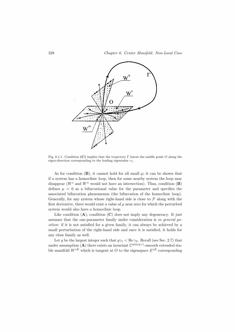
328 Chapter 6. Center Manifold. Non-Local Case
Fig. 6.1.1. Condition (C) implies that the trajectory Γ leaves the saddle point O along theeigen-direction corresponding to the leading eigenvalue γ1.
As for condition (B), it cannot hold for all small µ; it can be shown that
if a system has a homoclinic loop, then for some nearby system the loop may
disappear (W s and Wu would not have an intersection). Thus, condition (B)
defines µ = 0 as a bifurcational value for the parameter and specifies the
associated bifurcation phenomenon (the bifurcation of the homoclinic loop).
Generally, for any system whose right-hand side is close to F along with the
first derivative, there would exist a value of µ near zero for which the perturbed
system would also have a homoclinic loop.
Like condition (A), condition (C) does not imply any degeneracy. It just
assumes that the one-parameter family under consideration is in general po-
sition: if it is not satisfied for a given family, it can always be achieved by a
small perturbation of the right-hand side and once it is satisfied, it holds for
any close family as well.
Let q be the largest integer such that qγ1 < Re γ2. Recall (see Sec. 2.7) that
under assumption (A) there exists an invariant Cmin(q,r)-smooth extended sta-
ble manifold W sE which is tangent at O to the eigenspace EsE corresponding

6.1. Center manifold for a homoclinic loop 329
Fig. 6.1.2. The extended stable manifold W sE which contains the stable manifold W s and istangent at the saddle point to the eigenspace corresponding to the characteristic exponentsλn, . . . , λ1, γ1. The manifold W sE it is not unique; any two of such manifolds have a commontangent on W s. The strongly unstable sub-manifold W uu is uniquely embedded into thesmooth invariant foliation Fu on W u.
to the eigenvalues (λn, . . . , λ1, γ1). The manifold W sE contains entirely the
stable manifold W s. Though it is not defined uniquely, any two such manifolds
have the same tangent at any point of W s. Another important object (see
Sec. 5.4) is the smooth invariant foliation Fu on the unstable manifold W u
which includes the non-leading unstable manifold W uu among its leaves, see
Fig. 6.1.2.
The invariant extended stable manifold is defined locally, in a small neigh-
borhood of O. However, if we take a point belonging to a piece of the trajectory
Γ which belongs to W sloc, then a sufficiently small piece of W sE
loc that contains
this point may be continued by the backward trajectories of the system into
a small neighborhood of any prescribed preceding point on Γ, see Fig. 6.1.3.
In the same manner, the local strongly unstable foliation is extended by the
forward trajectories of the system into the entire unstable manifold.
Since Γ lies simultaneously in W u and in W s, each point of Γ belongs to
some piece of the extended stable manifold, and to some leaf of the strongly
unstable foliation. Therefore, the following requirement makes sense.
(D) The manifold W sE is transverse to the leaves of the foliation Fu at each
point of the homoclinic trajectory Γ.
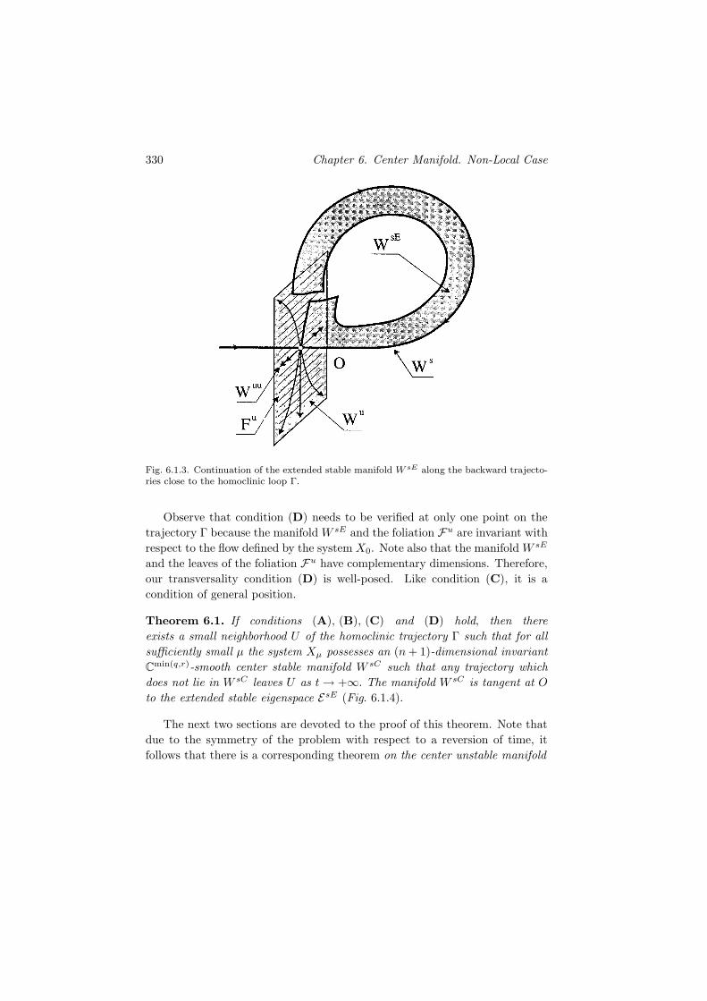
330 Chapter 6. Center Manifold. Non-Local Case
Fig. 6.1.3. Continuation of the extended stable manifold W sE along the backward trajecto-ries close to the homoclinic loop Γ.
Observe that condition (D) needs to be verified at only one point on the
trajectory Γ because the manifold W sE and the foliation Fu are invariant with
respect to the flow defined by the system X0. Note also that the manifold W sE
and the leaves of the foliation Fu have complementary dimensions. Therefore,
our transversality condition (D) is well-posed. Like condition (C), it is a
condition of general position.
Theorem 6.1. If conditions (A), (B), (C) and (D) hold, then there
exists a small neighborhood U of the homoclinic trajectory Γ such that for all
sufficiently small µ the system Xµ possesses an (n+ 1)-dimensional invariant
Cmin(q,r)-smooth center stable manifold W sC such that any trajectory which
does not lie in W sC leaves U as t→ +∞. The manifold W sC is tangent at O
to the extended stable eigenspace EsE (Fig. 6.1.4).
The next two sections are devoted to the proof of this theorem. Note that
due to the symmetry of the problem with respect to a reversion of time, it
follows that there is a corresponding theorem on the center unstable manifold

6.1. Center manifold for a homoclinic loop 331
Fig. 6.1.4. The center stable manifold W sC .
which may be formulated as follows. As above, suppose the system has a
homoclinic loop Γ at µ = 0. Let us modify conditions (A), (C) and (D) as
follows.
(A′) Let the characteristic exponents of the point O satisfy the following
condition:
Reλn ≤ · · · ≤ Reλ2 < λ1 < 0 < Re γ1 ≤ · · · ≤ Re γm .
In this case, since the leading stable eigenvalue λ1 is real, there exists an
(n− 1)-dimensional strongly stable sub-manifold W ss ⊂W s.
(C′) Assume that the homoclinic trajectory Γ does not lie in W ss.
(D′) Assume that at each point of Γ the extended unstable manifold W uE is
transverse to the leaves of the strongly stable foliation F s, see Fig. 6.1.5.
As in the above case we can continue the invariant extended unstable
manifold along the forward trajectories, see Fig. 6.1.6.

332 Chapter 6. Center Manifold. Non-Local Case
Fig. 6.1.5. The extended unstable manifold W uE contains W u and is tangent at the saddlepoint to the eigenspace corresponding to the characterstic exponents λ1, γ1, . . . , γm. Themanifold W uE is not unique; any two of such manifolds touch each other everywhere onW u. The strongly stable sub-manifold W ss is uniquely embedded into the smooth invariantfoliation F s on W s.
Fig. 6.1.6. Continuation of the extended unstable manifold W uE along the forward trajec-tories close to Γ.
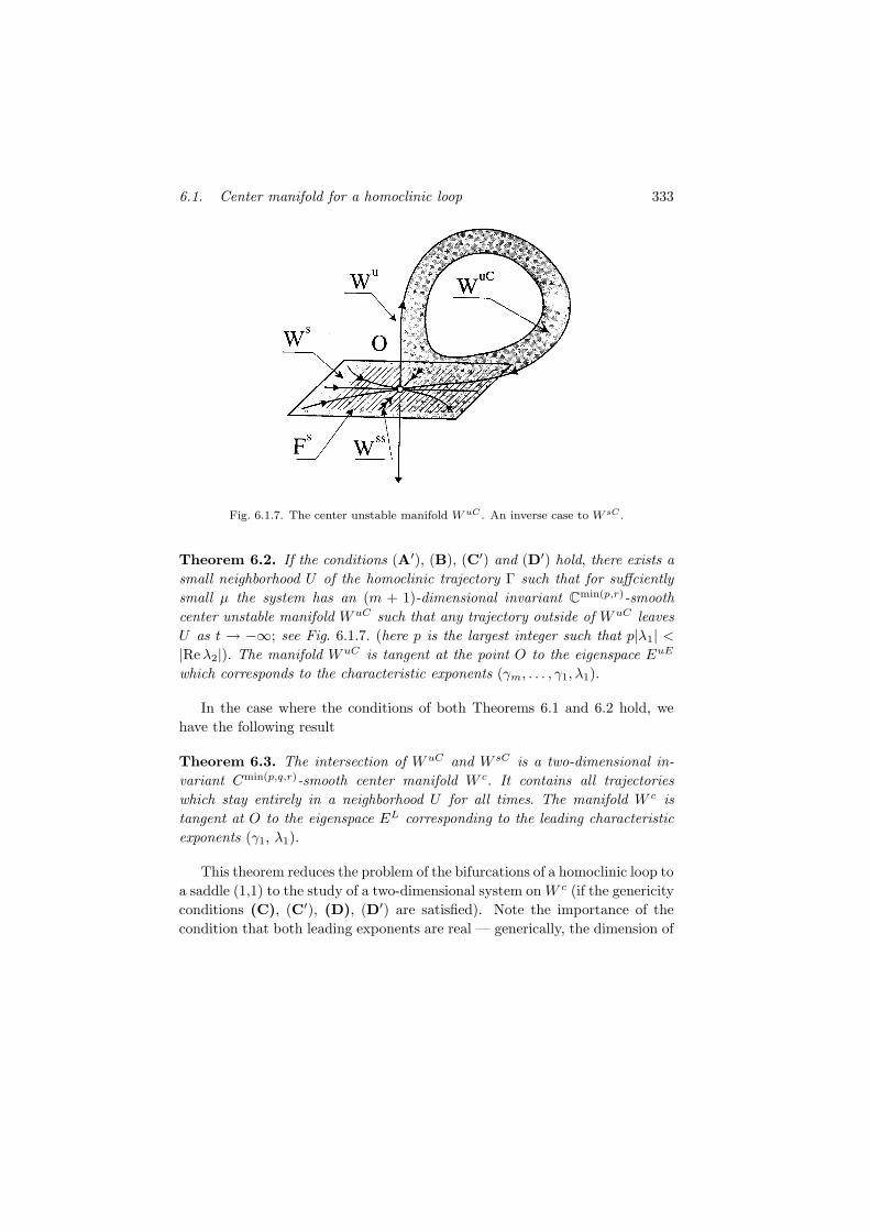
6.1. Center manifold for a homoclinic loop 333
Fig. 6.1.7. The center unstable manifold W uC . An inverse case to W sC .
Theorem 6.2. If the conditions (A′), (B), (C′) and (D′) hold, there exists a
small neighborhood U of the homoclinic trajectory Γ such that for suffciently
small µ the system has an (m + 1)-dimensional invariant Cmin(p,r)-smooth
center unstable manifold W uC such that any trajectory outside of W uC leaves
U as t → −∞; see Fig. 6.1.7. (here p is the largest integer such that p|λ1| <
|Reλ2|). The manifold W uC is tangent at the point O to the eigenspace EuE
which corresponds to the characteristic exponents (γm, . . . , γ1, λ1).
In the case where the conditions of both Theorems 6.1 and 6.2 hold, we
have the following result
Theorem 6.3. The intersection of W uC and W sC is a two-dimensional in-
variant Cmin(p,q,r)-smooth center manifold W c. It contains all trajectories
which stay entirely in a neighborhood U for all times. The manifold W c is
tangent at O to the eigenspace EL corresponding to the leading characteristic
exponents (γ1, λ1).
This theorem reduces the problem of the bifurcations of a homoclinic loop to
a saddle (1,1) to the study of a two-dimensional system on W c (if the genericity
conditions (C), (C′), (D), (D′) are satisfied). Note the importance of the
condition that both leading exponents are real — generically, the dimension of

334 Chapter 6. Center Manifold. Non-Local Case
the center manifold near a homoclinic loop is equal to the number of the leading
characteristic exponents (both negative and positive) and when this dimension
is greater than two, the bifurcations of such loop may be quite complicated in
some cases.
In the case of a homoclinic loop to a saddle-(1,1), the two-dimensional dy-
namics is relatively simple. Nevertheless, the reduction to the center manifold
requires some caution here. Our first observation is a low smoothness of W c.
Generally, it is only C1 and this may present an obstacle to a straightfor-
ward transcription of two-dimensional results into higher dimensions. Thus,
the two-dimensional theory of bifurcations of a homoclinic loop developed by
E. A. Leontovich produces a hierarchy of more and more degenerate cases
(corresponding to an increasingly large number of limit cycles appearing at bi-
furcation). The study of these cases requires an increasingly higher smoothness
of the system and, of course, the naive idea of simply repeating this hierar-
chy in the multidimensional situation, by referring to Theorem 6.3, would lead
to erroneous results. Unlike the case of local bifurcations, Theorems 6.1–6.3
essentially contain results of a qualitative rather than analytic nature.
Our second observation is that the manifold W c is not local (it is not
homeomorphic to a disc). Since its tangent at O is the leading plane EL, it
coincides locally with one of the saddle leading manifolds W Lloc. At µ = 0, this
manifold must contain a piece Γ+ of the homoclinic trajectory Γ which lies in
W sloc and a piece Γ− of Γ which lies inW u
loc. From a small neighborhood of Γ+ a
small piece of WLloc can be continued by the forward trajectories along the loop
Γ until it reaches Γ−. The manifold obtained as a result of continuation must
return to a neighborhood of O in such a way that it can be glued smoothly
at this moment to the same local manifold WLloc — in order that a smooth
invariant manifold WC can be formed. If the orientation is preserved, the
resulting glued manifold is a two-dimensional annulus. If not, the manifold
W c is a Mobius band. In fact, both cases are possible. Thus, in the multi-
dimensional case, the bifurcation of a homoclinic loop to a saddle-(1,1) are
reduced (generically) to a corresponding bifurcation either on the plane, or on
a two-dimensional non-orientable manifold.
6.2. The Poincare map near a homoclinic loop
In this and the next sections we present the proof of Theorem 6.1 which is
based on a study of the Poincare map T defined by the trajectories of the

6.2. The Poincare map 335
Fig. 6.2.1. The Poincare map represented as a superposition of two maps: the local map
Tloc defined along the trajectories from the cross-section Sin to Sout near the saddle pointO, and the global map Tglo defined by the trajectories starting from Sout and ending on Sin
along the global part of the homoclinic loop Γ.
system in a small neighborhood U of the homoclinic loop Γ. This map may
be represented as a superposition of two maps: a local map Tloc defined near
the saddle point O, and a global map Tglo defined by trajectories along the
global part of the homoclinic trajectory Γ outside a small neighborhood of the
saddle, see Fig. 6.2.1.
In a neighborhood of the saddle O let us introduce coordinates (u, y, w),
u ∈ Rn, y ∈ R
1 and w ∈ Rm−1 such that locally, the system assumes the form
u = Au+ f(u, y, w, µ) ,
y = γy + g(u, y, w, µ) ,
w = Bw + h(u, y, w, µ) ,
(6.2.1)
where A is an (n× n)-matrix and spectrA = λ1, . . . , λn, B is an (m− 1) ×
(m− 1)-matrix and spectrB = γ2, . . . , γm, and γ ≡ γ1. Let us choose some
λ > 0 and η > 0 such that
maxReλ1, . . . ,Reλn < −λ (6.2.2)
minRe γ2, . . . ,Re γm > η > γ . (6.2.3)

336 Chapter 6. Center Manifold. Non-Local Case
The functions f , g, h are Cr-smooth and
(f, g, h)(0, 0, 0, 0) = 0 ,∂(f, g, h)
∂(u, y, w, µ)
∣∣∣∣(x,y,z,µ)=0
= 0 . (6.2.4)
In these coordinates, at µ = 0, the stable manifold is tangent at O to the
space (y, w) = 0, the unstable manifold is tangent to u = 0 and the strong
unstable manifold is tangent to (u,w) = 0.
At µ = 0 the homoclinic trajectory Γ returns to a small neighborhood of
O as t→ +∞, lying in the local stable manifold. Therefore, for some small ξ,
the trajectory intersects the surface ‖u‖ = ξ at some point M+ ∈ W sloc. Let
us denote the coordinates of M+ as (u+, y+, w+) see Fig. 6.2.1. Choose some
small δ > 0 and consider a small area
Sin =‖u‖ = ξ,
∥∥(u− u+, y − y+, w − w+
)∥∥ ≤ δ
. (6.2.5)
It follows from Theorem 2.4 that ddt‖u‖ < 0 on W s
loc; i.e. ‖u‖ strictly decreases
along the trajectories in W sloc. This implies that for a sufficiently small ξ the
surface ‖u‖ = ξ is transverse to the trajectories on W sloc and, therefore, to all
close orbits. Consequently, being a part of this cross-section, the area S in is
transverse to the trajectories close to Γ provided that µ is sufficiently small.
Since the trajectory Γ does not lie in the non-leading unstable sub-manifold
Wuu (condition (C) of Theorem 6.1), it leaves the saddle O along the leading
direction which coincides with the y-axis. Without loss of generality, we can
assume that Γ leaves O towards positive values of y. In this case, for sufficiently
small y− > 0, the homoclinic trajectory penetrates the surface y = y− at
some point M− ∈ Wuloc. Denote M− = (u−, y−, w−). Since at µ = 0 the
trajectory Γ is transverse to y = y−, it follows that at all small µ the small
area
Sout =y = y−,
∥∥(u− u−, w − w−
)∥∥ ≤ δ
, (6.2.6)
is a cross-section (i.e. it intersects the trajectories of the system transversely).
At µ = 0, the trajectory of M− (the trajectory Γ) reaches the point M+ at
some finite positive time. Therefore, due to the continuous dependence of the
trajectories on initial conditions and parameters, for all small µ the trajectories
which start on Sout near M− must intersect Sin near M+. Thus, we can define
the map Tglo which maps a small neighborhood of M− on Sout into a small
neighborhood of M+ on Sin.

6.2. The Poincare map 337
All trajectories starting on Sin enter an ξ-neighborhood of the saddle point
O. If a trajectory does not belong to the local stable manifold, it leaves a
small neighborhood of O after some time. If a trajectory starting at some
point M0 ∈ Sin leaves a small neighborhood of the saddle at a point M 1
which belongs to Sout we will say that M0 and M1 are related by the local
map Tloc : M0 7→M1.
Obviously, a trajectory which stays for all positive times in a small neigh-
borhood of the homoclinic loop must intersect Sin and Sout: after leaving a
neighborhood of the origin it must traverse along the global piece of Γ and
then return into a neighborhood of the origin across Sin, and after entering
this neighborhood at some point on Sin, it may leave only at some point on
Sout (or it may stay in a small neighborhood of O for all times thereafter
— it belongs to W sloc in this case). By definition, the consecutive points of
intersection of a trajectory with the cross-sections are related by the map Tloc,
or by Tglo. Thus, there is a correspondence between the trajectories under
consideration and the iterations of the map T = Tglo Tloc.
Because the flight time from Sout to Sin is bounded, the map Tglo is a
Cr-diffeomorphism. Therefore, the necessary estimates on the map Tglo can
be obtained simply by Taylor series expansion. We postpone the study of the
global map to the end of this section and consider now the question on the
structure of the local map which is much less trivial (because the time the
trajectory spends in a small neighborhood of O before it reaches Sout may be
unboundedly large, and tends to infinity as the starting point tends to W sloc).
To overcome the difficulties we use the method of the boundary-value problem
described in Sec. 2.8 and in Sec. 5.2.
Let us denote the coordinates on Sin as (u0, y0, w0) (‖u0‖ = ξ) and the
coordinates on Sout as (u1, w1). Let y = ψs(u, µ), w = ϕs(u, µ) be the
equation of W sloc and u = ψu(y, w, µ) be the equation of W u
loc. Also let
w = ϕsE(u, y, µ) be the equation of the local extended stable manifold W sEloc .
Denote by luu that leaf of the extended unstable foliation which passes through
the point M−. Let y = ψuu(w, µ), u = ϕuu(w, µ) be the equation of luu.
Lemma 6.1. There exist functions uloc and wloc defined on ‖u0 − u+‖ ≤
δ, ‖w1 −w−‖ ≤ δ and 0 < y0 −ψs(u0, µ) ≤ δ′ for some small δ′, such that for
two points M0 ∈ Sin and M1 ∈ Sout, the relation M1 = TlocM0 holds if and
only if
u1 = uloc(u0, y0, w1, µ) , w0 = wloc(u
0, y0, w1, µ) . (6.2.7)

338 Chapter 6. Center Manifold. Non-Local Case
The functions uloc and wloc satisfy the following inequalities∥∥∥∥
∂uloc∂(u0, y0)
∥∥∥∥≤ C e(γ−λ+ε)τ , (6.2.8)
∥∥∥∥
∂uloc∂µ
∥∥∥∥≤ C max
1, eγ−λ+ε)τ
, (6.2.9)
∥∥∥∥
∂uloc∂ω1
∥∥∥∥≤ C , (6.2.10)
∥∥∥∥
∂ωloc∂(u0, y0, µ)
∥∥∥∥≤ C , (6.2.11)
∥∥∥∥
∂ωloc∂ω1
∥∥∥∥≤ C e−(η−γ−ε)τ , (6.2.12)
where C is some positive constant, λ, η and γ satisfy conditions (6.2.2) and
(6.2.3), a small positive ε can be made arbitrarily small if δ is sufficiently small.
Here τ(y0, u0, w1, µ) is the flight time from M0 to M1; it tends to infinity as
y0 → ψs(u0, µ) and∥∥∥∥
∂γ
∂(u0, y0, µ)
∥∥∥∥≤ C e(γ+ε)τ ,
∥∥∥∥
∂γ
∂ω1
∥∥∥∥≤ C . (6.2.13)
Furthermore,
limy0→ψs(u0,µ)
uloc = ψu(y−, w1, µ) ,
limy0→ψs(u0,µ)
wloc = ψs(u0, µ) ,
limy0→ψs(u0,µ)
∂uloc∂w1
=∂ψu
∂w(y−, w1, µ) ,
limy0→ψs(u0,µ)
∂uloc∂µ
=∂ψu
∂µ(y−, w1, µ) if γ < λ ,
limy0→ψs(u0,µ)
∂wloc∂(u0, y0, µ)
=∂ϕsE
∂(u, y, µ)(u0, y0, µ) .
(6.2.14)
Proof. As show in Sec. 2.7, for any positive τ > 0 and for any small
(u0, y1, w1) there is a unique trajectory (u∗(t), y∗(t), w∗(t)) of the system which

6.2. The Poincare map 339
lies in a small neighborhood of the origin and which represents a solution of
the boundary-value problem:
u∗(0) = u0 , y∗(τ) = y1 , w∗(τ) = w1 .
Thus, the trajectory from a point M 0 reaches a point M1 at the moment t = τ
if and only if
u1 = u∗(τ ;u0, y1, w1, µ, τ) ,
y0 = y∗(0;u0, y1, w1, µ, τ) ,
w0 = w∗(0;u0, y1, w1, µ, τ)
(6.2.15)
(we took into account the fact that the solution (u∗, y∗, w∗) depends on the
boundary data (u0, y1, w1), on the flight time τ , and on µ; as shown in Sec. 2.8
the dependence is Cr-smooth with respect to all variables). The boundary
value problem under consideration is a special case of the boundary-value prob-
lem considered in Sec. 5.2: one should consider u as the z-variable, and (y, w)
as the v-variable in terms of that section. The estimates of Theorem (5.12)
give in our case (one should assume α = λ and β = γ − ε in (5.2.27))
∥∥∥∥
∂u∗
∂(u0, τ)
∥∥∥∥≤ C e−λτ ,
∥∥∥∥
∂u∗
∂(w1, µ)
∥∥∥∥≤ C
∥∥∥∥
∂(y∗, w∗)
∂(y1, w1, τ)
∥∥∥∥≤ C e−(γ−ε)τ ,
∥∥∥∥
∂(y∗, w∗)
∂(u0, µ)
∥∥∥∥≤ C
(6.2.16)
(here, we calculate the derivatives of (y∗, w∗) at t = 0, by formula (5.2.27a),
and the derivatives of u∗ at τ − t = 0, by formula (5.2.27b)).
As we argued in Sec. 2.8, the limit τ = +∞ corresponds to M 0 ∈W sloc and
M1 ∈Wuloc; i.e.
y∗ |τ=+∞ = ψs(u0, µ) ,
w∗ |τ=+∞ = ϕs(u0, µ) ,
u∗ |τ=+∞ = ψu(y1, w1, µ) .
(6.2.17)

340 Chapter 6. Center Manifold. Non-Local Case
Moreover,
∂y∗
∂(u0, µ)
∣∣∣∣τ=+∞
=∂ψs
∂(u0, µ)(u0, µ) ,
∂w∗
∂(u0, µ)
∣∣∣∣τ=+∞
=∂ϕs
∂(u0, µ)(u0, µ) ,
∂u∗
∂(y1, w1, µ)
∣∣∣∣τ=+∞
=∂ψu
∂(y1, w1, µ)(y1, w1, µ) .
(6.2.18)
At the same time one may write
u1 = u∗∗(τ ;u0, y0, w1, µ, τ) ,
y1 = y∗∗(τ ;u0, y0, w1, µ, τ) ,
w0 = w∗∗(0;u0, y0, w1, µ, τ)
(6.2.19)
where (u∗∗(t), y∗∗(t), w∗∗(t)) is the solution of the boundary-value problem
u∗∗(0) = u0 , y∗∗(0) = y0 , w∗∗(τ) = w1 (6.2.20)
for a system obtained from (6.2.1) via a continuation from a small neighbor-
hood of the origin onto the whole space Rn+m (note that once (6.2.15) is
satisfied, the solution stays in a small neighborhood of the origin and when ap-
plying the results of Sec. 5.2 concerning the boundary-value problem (6.2.20)
we should not worry about the influence of this continuation). The prob-
lem (6.2.20) is a particular case of the boundary-value problem considered in
Secs. 5.2, 5.3: now one should denote the variables (u, y) as the z-variable
and w as the v-variable and assume α = γ + ε and β = η. The estimates of
Theorem 5.12 give for this case (see (5.2.26a) and (5.2.26b))
∥∥∥∥
∂(y∗∗, u∗∗)
∂(u0, y0, µ, τ)
∥∥∥∥≤ C e(γ+ε)τ ,
∥∥∥∥
∂(y∗∗, u∗∗)
∂w1
∥∥∥∥≤ C
∥∥∥∥
∂w∗∗
∂(w1, τ)
∥∥∥∥≤ C e−ητ ,
∥∥∥∥
∂w∗∗
∂(u0, y0, µ)
∥∥∥∥≤ C
(6.2.21)

6.2. The Poincare map 341
(we calculate here the derivatives of w∗∗ at t = 0, from formula (5.2.26a), and
the derivatives of (u∗∗, y∗∗) at τ − t = 0, from formula (5.2.26b)).
The limit τ = +∞ was considered in Sec. 5.3. According to Lemma 5.3,
the derivatives of w∗∗ in the limit τ = +∞ coincide with the derivatives of the
function whose graph is the conventionally stable manifold of the limiting point
M0. Since the point M0 belongs to W sloc(O) at τ = +∞, its conventionally
stable manifold coincides with the conventionally stable manifold of O — in
our case it is the extended stable manifold of W sE . Thus,
∂w∗∗
∂(u0, y0, µ)
∣∣∣∣τ=+∞
=∂ϕsE
∂(u0, y0, µ)(u0, ψs(u0, µ) , µ) . (6.2.22)
Due to the general symmetry of the problem with respect to a reversion in
time (see remarks in the proof of Theorem 5.12) the derivatives of u∗∗ and y∗∗
in the limit τ = +∞ coincide with the derivatives of the function whose graph
is the conventionally unstable manifold of the limiting point M 1 — in our case
it is the leaf luu of the strongly unstable foliation through M 1. Thus,
∂(y∗∗, u∗∗)
∂w1
∣∣∣∣τ=+∞
=∂(ψuu, ϕuu)
∂w1(w1, µ) . (6.2.23)
Fixing the value of y1 = y− which corresponds to M1 ∈ Sout one may look
at the second equation in (6.2.15) as an implicit equation for determining the
flight time τ from M0 to M1. We will prove at once that the derivative ∂y∗
∂τ
does not vanish (and it is negative). Therefore, the equation
y0 = y∗(0;u0, y−, w1, µ, τ) (6.2.24)
can be solved with respect to τ : the value τ = +∞ corresponds to y0 =
ψs(u0, µ) and since ∂y∗
∂τ < 0, a decrease in τ to a finite value is followed by a
monotonic increase in y0. Thus, this equation uniquely defines the flight time
as a function of (u0, y0, w1, µ) at y0 varying from ψs(u0, µ) to ψs(u0, µ) + δ′
for some sufficiently small δ′. Substituting the expression for τ into u∗ and
w∗∗ would give the desired functions uloc and wloc (having fixed y1 = y−
and ‖u0‖ = ξ = ‖u+‖).
By (6.2.24)
∂τ
∂y0=
(∂y∗
∂τ
)−1
,
∂τ
∂(u0, w1, µ)= −
(∂y∗
∂τ
)−1∂y∗
∂(u0, w1, µ).
(6.2.25)

342 Chapter 6. Center Manifold. Non-Local Case
To estimate these derivatives, let us compare the second equation of (6.2.15)
with the second equation in (6.2.19). We immediately have
1 =∂y∗
∂y1
∂y∗∗
∂y0,
0 =∂y∗
∂(u0, w1, µ)+∂y∗
∂y1
∂y∗∗
∂(u0, w1, µ).
(6.2.26)
Note also that according to Lemma 5.1,
∂y∗
∂τ= −
∂y∗
∂y1y
∣∣∣∣M1
−∂y∗
∂w1w|M1 .
It follows from this equation and from (6.2.25) and (6.2.26) that
∂τ
∂(u0, y0, w1, µ)= −
∂y∗∗
∂(u0, y0, w1, µ)
/(
y|M1 −∂y∗∗
∂w1w
∣∣∣∣M1
)
. (6.2.27)
Note that the denominator in this formula does not vanish (it is positive).
Indeed, since the trajectory Γ does not belong to W uu, it leaves the origin
tangentially to the y-axis (see Theorem 2.5). Hence, the value of w− is much
less than y−. In particular, this means that y|M1 ‖w‖M1 and our claim
follows from the boundedness of ∂y∗∗
∂w1 (note that y|M1 is positive since it is
equal essentially to γy−, and y− is positive).
Thus, the inverse ∂τ∂y0 to ∂y∗
∂τ exists which proves that the flight time is
indeed uniquely defined by (u0, y0, w1, µ). The required negativeness of ∂τ∂y0
follows from formula (6.2.27): ∂y∗∗
∂y0 is equal, by definition, to 1 at τ = 0 and
since this derivative cannot vanish at any τ (by virtue of the first equation in
(6.2.26)) it remains positive for all τ .
From the relations (6.2.27) and (6.2.21) we obtain the inequality (6.2.13).
The functions uloc and wloc are defined as
uloc(u0, y0, w1, µ) ≡ u∗(τ(u0, y0, w1, µ);u0, y−, w1, µ, τ(u0, y0, w1, µ))
wloc(u0, y0, w1, µ) ≡ w∗∗(τ(u0, y0, w1, µ);u0, y0, w1, µ, τ(u0, y0, w1, µ)) .
(6.2.28)
One may check now that the estimates (6.2.16), (6.2.21) and (6.2.13) imply
(6.2.8)–(6.2.12) and the limit relations (6.2.18), (6.2.22) and (6.2.23) im-
ply (6.2.14). This completes our proof of the lemma.

6.2. The Poincare map 343
The higher derivatives of the functions uloc and wloc, can also be easily esti-
mated using Theorem 5.12 and the identities (6.2.28) and (6.2.27) (in (6.2.27),
the values of y and w at the point M 1(u1, y−, w1) are evaluated by formulas
(6.2.1)). Omitting the obvious calculations the final result is as follow:
Lemma 6.2. In Lemma 6.1 the following estimates hold:
∥∥∥∥
∂|k1|+|k2|+|k3|uloc∂(u0, y0)k1∂µk2∂(w1)k3
∥∥∥∥≤ C e((|k1|+|k2|)(γ+ε)−λ)τ (k1 6= 0) ,
∥∥∥∥
∂|k2|+|k3|uloc∂µk2∂(w1)k3
∥∥∥∥≤ C max
(1, e(|k2|(γ+ε)−λ)τ
),
∥∥∥∥
∂|k1|+|k2|wloc∂(u0, y0, µ)k1∂(w1)k2
∥∥∥∥≤
C if k2 = 0 and
|k1|(γ + ε) < η ,
C e−(η−|k1|(γ+ε))τ if k2 6= 0 or
|k1|(γ + ε) > η .
(6.2.29)
We remark that as in Lemma 6.1, those derivatives which are bounded by a
constant in these formulae have, in fact, a finite limit, equal to the derivatives
of the corresponding conventionally stable manifolds, as τ → +∞ (see remarks
after Lemma 5.3).
The estimates in Lemmas 6.1 and 6.2 are more than enough for our pur-
poses. In fact, what we need to prove the invariant manifold theorem is sum-
marized by the following lemma.
Lemma 6.3. Let us change the coordinates on the cross-sections S in and Sout
in the following way:
y0new = y0 − ψs(u0, µ) ,
w0new = w0 − ϕsE(u0, y0, µ) on Sin
u1new = u1 − ψu(y1, w1, µ) on Sout
(we straighten the intersections W sloc∩S
in and Wuloc∩S
out and make the inter-
section W sEloc ∩ Sin tangent to w0 = 0 at the point M+ = Γ ∩ Sin at µ = 0).
Points M0 ∈ Sin and M1 ∈ Sout are related by the map Tloc if, and only if,
u1 = uloc(u0, y0, w1, µ) , w0 = wloc(u
0, y0, w1, µ) (6.2.30)

344 Chapter 6. Center Manifold. Non-Local Case
where the functions uloc and wloc are now defined at y0 ∈ [0, δ′]; they satisfy
the following inequalities in the new coordinates:
∥∥∥∥
∂|k1|+|k2|uloc∂(u0, y0, µ)k1∂(w1)k2
∥∥∥∥≤ C e|k1|(γ+ε)τ , (k1 6= 0) ,
∥∥∥∥
∂|k1|+|k2|wloc∂(u0, y0, µ)k1∂(w1)k2
∥∥∥∥≤ C e−(η−|k1|(γ+ε))τ , (k2 6= 0) .
(6.2.31)
All derivatives∂|k|uloc
∂(w1)k and∂|k|wloc
∂(u0,y0,µ)k up to order min(q, r) are continuous
and bounded where r is the smoothness of the system and q is the largest integer
such that qγ < η. Moreover, in the new coordinates
uloc(u0, 0, w1, µ) ≡ 0 , wloc(u
0, 0, w1, µ) ≡ 0 (6.2.32)
and∂kwloc
∂(u0, y0, µ)k(u0, 0, w1, µ) ≡ 0 , (6.2.33)
at k ≤ min(q, r).
This lemma follows immediately from the two previous lemmas. Observe
that it follows from (6.2.32) that
∂uloc∂w1
≡ 0 at y0 = 0 . (6.2.34)
Let us now consider the global map Tglo : Sout 7→ Sin. Since the flight time
from Sin to Sout is bounded (and it depends smoothly on the initial point)
the map Tglo is a Cr-diffeomorphism. Somehow, it is more convenient for us
to consider the inverse map T−1glo . Since it is C
r-smooth as well, one may write
near the point M+ the map T−1glo : Sin → Sout in the form
(u1 − u−(µ)w1 − w−(µ)
)
=
(d11 d12 d13
d21 d22 d23
)
u0 − u+
y0
w0
+
(uglo(u
0, y0, w0, µ)wglo(u
0, y0, w0, µ)
)
. (6.2.35)
Here (u−(µ), w−(µ)) are the coordinates of the image T−1gloM
+ of the point
M+. At µ = 0 it is the point M− = Γ ∩ Sout. Recall that in the coordinates

6.3. Proof of the center manifold theorem near a homoclinic loop 345
of Lemma 6.3 u−(0) = 0. The constants d11, d12, d13, d21, d22 and d23 are
matrices of dimensions n×(n−1), n×1, n×(m−1), (m−1)×(n−1), (m−1)×1
and (m − 1) × (m − 1), respectively; the functions uglo and wglo denote the
nonlinear terms.
Recall that by assumption the manifold W sE intersects transversely the
leaves of the strongly unstable foliation (condition (D)) at the points of Γ at
µ = 0. Therefore, the intersection of the tangent to the continuation of W sE
at the point M− with the tangent to the leaf luu at the same point is zero.
The tangent to W uloc at this point is spanned to the tangent to luu and to the
phase velocity vector (u, y, w)|M− which is tangent to Γ at M−. This vector
is also contained in the tangent to W sE (because W sE contains Γ). Thus, the
intersection of the tangents to W sE and Wuloc at M− is one-dimensional (it is
spanned on the phase velocity vector). This implies that W sE and Wuloc meet
transversely at M−. Therefore, the image of W sEloc ∩S
in by the map T−1glo must
be transverse to the intersection W uloc ∩S
out. In the coordinates of Lemma 6.3
the latter is given by u1 = 0 and W sEloc ∩S
in is tangent to w0 = 0 at µ = 0.
Therefore, the transversality condition (D) transcripts in these coordinates as
a transversality of the space
u1 = (d11(0), d12(0)) ·
(u0 − u+
y0
)
with respect to the space u1 = 0, which means that
det (d11, d12) 6= 0 . (6.2.36)
6.3. Proof of the center manifold theorem near ahomoclinic loop
In order to prove Theorem 6.1, we must establish the existence of an invariant
manifold for the inverse of the Poincare map T−1 = T−1glo T−1
loc on the cross-
section Sin. We achieve this by using Theorem 4.4 (a generalization of the
annulus principle).
Recall (see Lemma 6.3) that we have represented the map Tloc : M0 7→M1
in the cross-form by terms of the functions uloc and wloc which are defined
for ‖u0 − u+‖ ≤ δ, ‖w1‖ ≤ δ, y0 ∈ [0, δ′] for some small δ and δ′. The map
T−1glo is given by formula (6.2.35). It follows from the superposition of these

346 Chapter 6. Center Manifold. Non-Local Case
two maps that two points (u0, y0, w0) and (u0, y0, w0) are related by the map
T−1 : (u0, y0, w0) 7→ (u0, y0, w0) if, and only if,
w0 = wloc(u0, y0, w1, µ) ,
u1 = uloc(u0, y0, w1, µ) ,
u1 − u−(µ) = d11(u0 − u+) + d12y
0 + d13w0 + uglo(u
0, y0, w0, µ) ,
w1 − w−(µ) = d21(u0 − u+) + d22y
0 + d23w0 + wglo(u
0, y0, w0, µ) ,
(6.3.1)
where (u1, w1) is an intermediate point where the backward trajectory of the
point (u0, y0, w0) intersects Sout.
Let us extend the domain of the functions involved here in the following
way. First, let us assume (uloc, wloc) ≡ 0 for y0 ≤ 0, and then change these
functions by multiplying them by some factor which vanishes outside a small
neighborhood of (u+, 0, 0):
uloc → uloc · χ
(‖u0 − u+, y0, w1‖
ρ
)
,
wloc → wloc · χ
(‖u0 − u+, y0, w1‖
ρ
)
,
where χ is a Cr-smooth function such that
χ(s) =
1, if s ≤ 1/2 ,
0, if s ≥ 1 ,and
∣∣∣∣
∂χ
∂s
∣∣∣∣< 3 . (6.3.2)
Here ρ is a small constant. One can see that such multiplications do not change
the estimates of Lemma 6.3 in an essential way, just an additional constant
factor may appear. Observe that the functions uloc and wloc are kept the same
in a small ρ2 -neighborhood of (u+, 0, 0) whereas they now vanish identically on
the boundary of the domain of definition, whence we may consider them to be
identically zero outside, without any loss of smoothness.
The same procedure may be applied to the map T−1glo — the functions uglo
and wglo may be modified outside the ρ2 -neighborhood of the point (u0 =
u+, y0 = 0, w0 = 0) so that they vanish at a distance ρ of that point, and this
allows one to assume that T−1glo is defined at all (u0, y0, w0). Recall that uglo
and wglo are nonlinear functions. Hence, if ρ is sufficiently small, then the
modified map T−1glo is very close to its linear part everywhere.

6.3. Proof of the center manifold theorem near a homoclinic loop 347
In particular, this means (by virtue of the transversality condition (6.2.42))
that the third equation in (6.3.1) can be solved with respect to (u0, y0) as
follows:
(u0, y0) = f(u1, w0, µ) , (6.3.3)
where f is some smooth function all of whose derivatives are uniformly
bounded. Consequently, the fourth equation in (6.3.2) can be recast into the
form
w1 = g(u1, w0, µ) , (6.3.4)
where g is a smooth function with the uniformly bounded derivatives. Substi-
tuting the last equation into the second equation of (6.3.1) we obtain
u1 = uloc(u0, y0, g(u1, w0, µ), µ) .
Since∂uloc
∂w1 tends to zero for small y0 (see Lemma 6.3), this derivative can be
made uniformly small for the modified function uloc by taking ρ small enough.
Therefore, the equation above can be solved with respect to u1. This gives
u1 = uloc(u0, y0, w0, µ) , (6.3.5)
where the function uloc essentially satisfies the same estimates (given by a
Lemma 6.3) as the function uloc.
The substitution of this expression into (6.3.3) and into the first equation
of (6.3.1) represents the map T−1 in the cross-form
w0 = F (w0, (u0, y0)) ,
(u0, y0) = G(w0, (u0, y0)) .(6.3.6)
One can see, using the estimates of Lemma 6.3, that the functions F and G
satisfy the conditions of Theorem 4.4 (under the weakened smoothness condi-
tions given below that theorem; observe that the function uloc is not smooth
at y0 = 0). Thus, we immediately have the existence of a Cmin(q,r)-smooth
manifold w0 = φ∗(u0, y0, µ) which is invariant with respect to the modified
map T−1. The function φ∗ is defined at all u0, y0, µ. Since the modified map
coincides with the original map T−1 in a small neighborhood of (u+, 0, 0) at
y0 ≥ 0, it follows that the intersection of the above manifold with this domain
is a smooth invariant manifold of the original map.
By construction (see the proof of the annulus principle in Sec. 4.2), forward
iterations of any point by the modified map T−1 converge exponentially to

348 Chapter 6. Center Manifold. Non-Local Case
the “large” invariant manifold we found. This implies that all points whose
backward iterations are at a bounded distance on this manifold must lie in
this manifold. In terms of the original Poincare map T this means that all
trajectories whose forward iterations lie in a small neighborhood of the point
(u0, 0, 0) must belong to the “small” invariant manifold.
The set of trajectories which start from points of this manifold on the
cross-section is an invariant manifold for the system of differential equations
under consideration (one should choose the pieces of the trajectories until they
remain in a small neighborhood U of the homoclinic loop). By construction,
this manifold contains all trajectories which stay in U for all positive times.
In particular, it contains the intersection W sloc ∩ U . The point O must also be
included in the resulting invariant manifold. Note that the smoothness of the
above invariant manifold follows from the proven smoothness of its intersection
with the cross-section Sin — everywhere except at the equilibrium state O.
The smoothness of O must be verified separately, but we refrain from giving a
complete proof here because it is irrelevant for our purposes. Just note that the
resulting invariant manifold coincides locally with one of the extended stable
manifolds W sEloc (O) from which the smoothness at O follows.
6.4. Center manifold theorem for heteroclinic cycles
The non-local center manifold theorem which we have proved for a homoclinic
loop admits a straightforward generalization onto a class of heteroclinic cycles.
Namely, suppose a family of Cr-smooth dynamical systems
x = X(x, µ) (6.4.1)
depending smoothly on some vector of parameters µ has a number of saddle
equilibrium states O1, . . . , Ok which satisfy condition (A) of the previous sec-
tions: for each saddle the leading positive characteristic exponent is real and
simple. Let the stable manifold of each Oi be n-dimensional and the unsta-
ble manifold be m-dimensional. Suppose that at µ = 0, for each i = 1, . . . , k
there exists a trajectory Γi of intersection W u(Oi) ∩Ws(Oi+1) (respectively,
Wu(Ok) ∩Ws(O1) for i = k).
The trajectories Γi are called heteroclinic because Γi tends to Oi as t →
−∞ (it lies in W u(Oi)) but it tends to another equilibrium state Oi+1 as
t → +∞ (it lies in W s(Oi+1)). The union C = O1 ∪ Γ1 ∪ O2 ∪ · · · ∪ Ok ∪ Γkis called a heteroclinic cycle or a heteroclinic contour. Note that generically

6.4. Center manifold for heteroclinic cycles 349
k-independent governing parameters µ1, . . . , µk are necessary for the system
to have the cycle with k-heteroclinic trajectories.
Let us impose on the trajectories Γi the same genericity conditions given
by conditions (C) and (D) of the previous sections. Namely,
For each heteroclinic trajectory Γi, suppose that it does not lie in the
non-leading unstable submanifold W uu(Oi), and suppose that the ex-
tended stable manifold W sE(Oi+1) is transverse to the leaves of the
strongly unstable foliation Fu(Oi) of Wu(Oi) at each point of the hete-
roclinic trajectory Γi (for each i = 1, . . . , k).
Theorem 6.4. There exists a small neighborhood U of the heteroclinic cycle
C such that for all sufficiently small µ the system possesses an (n+ 1)-dimen-
sional invariant Cq-smooth1 center stable manifold W sC such that any trajec-
tory which does not lie in W sC leaves U as t → +∞. The manifold W sC is
tangent at Oi to the extended stable eigenspace EsE(Oi).
The proof is identical to that of Theorem 6.1. One may construct a local
cross-section S(i)in to each Γi near Oi+1. Then, consider the inverse Ti : S
(i)in →
S(i−1)in of the Poincare map (the map Ti is defined by the backward trajectories
of the system). The maps Ti can be modified exactly in the same way as in
Sec. 6.3 and, after that, they are written in the cross-form
wi−1 = Fi(wi, (ui−1, yi−1), µ) ,
(ui, yi) = Gi(wi, (ui−1, yi−1), µ) ,(6.4.2)
where the w-variables belong to Rm−1, the (u, y)-variables to Rn and the func-
tions Fi, Gi satisfy the conditions of Theorem 4.4. One can check that denoting
x = (w1, . . . , wk) and y = ((u1, y1), . . . , (uk, yk);µ) the relations (6.4.2) (along
with the artificial equation µ = µ) define a cross-map
x = F (x, y)
y = G(x, y)(6.4.3)
which satisfy the conditions of Theorem 4.4. Thus, there exists a smooth
invariant manifold of the kind
(w1, . . . , wk) = ϕ∗((u1, y1), . . . , (uk, yk);µ) .
1The integer q must satisfy q ≤ r and qγ(i)1 < Re γ
(i)2 for all Oi, where γ
(i)1 is the leading
positive characteristic exponent of Oi and γ(i)2 is the next positive exponent.

350 Chapter 6. Center Manifold. Non-Local Case
We need somewhat more: each wi here should only depend on (ui, yi, µ). The
graphs L∗i of these dependencies would define the invariant manifold on the
extended cross-sections S(i)in :
TiL∗i = L∗
i−1 .
To prove that the invariant manifold of the map (6.4.3) has the required
structure, it is sufficient to note that the invariant manifold is obtained in
Theorem 4.4 as the limit of the iterations of an arbitrary Lipschitz manifold.
Thus, if we make as our initial guess the manifold, say, (w1 = 0, . . . , wk = 0)
which indeed represents the collection of independent surfaces on S(1)in , . . . , S
(k)in ,
respectively, then just by the essence of the problem all iterations will have the
same structure. Hence their limit will also have the same structure.
The intersection of the derived surfaces L∗i with the original local pieces of
the cross-sections S(i)in define the invariant manifold for the original Poincare
map. So, the set of trajectories which start on any of these surfaces is the
desired invariant manifold of the system itself.
Note that a reversion of time allows one to obtain an analogous center
unstable manifold theorem for the case when the leading negative exponent is
real and simple for each Oi, and a theorem on two-dimensional center manifold
when both positive and negative leading exponents are real and simple, as was
done in Sec. 6.1 for a homoclinic loop.
The heteroclinic cycles under consideration represents one of the simplest
cases among a large variety of possible heteroclinic or homoclinic structures.
For example, a single saddle equilibrium state may have more than one homo-
clinic loop at some value of µ (in a two-parameter family). We distinguish two
generic cases here:
• a figure-eight — the homoclinic trajectories Γ1 and Γ2 enter the saddle
O from the opposite directions, as shown in Fig. 6.4.1,
• a homoclinic butterfly — the homoclinic trajectories Γ1 and Γ2 come
back to O along the same direction (positive y), so they are tangent to
each other at O (as t→ +∞) as shown in Fig. 6.4.2.
Note that both cases correspond to the case where condition (C) holds for
both homoclinic trajectories: they do not belong to W uu and therefore leave
O along the leading direction, namely the y-axis.

6.4. Center manifold for heteroclinic cycles 351
Fig. 6.4.1. The homoclinic figure-eight for which the non-coincidence conditions are fulfilled:the separatrix Γ1 intersects only those strongly stable leaves which are not intersected bythe separatrix Γ2.
Fig. 6.4.2. The homoclinic butterfly composed by two loops Γ1 and Γ2 which does not satisfythe non-coincidence conditions: the strongly stable leaf of an arbitrary point P1 ∈ Γ1 lyingnear the equilibrium state coincides with the strongly stable leaf of some point P2 ∈ Γ2.

352 Chapter 6. Center Manifold. Non-Local Case
Suppose that the transversality condition (D) is fulfilled for both homo-
clinic trajectories (see Sec. 6.1). Again, revisiting the construction of the
previous section one may prove the following result.
Theorem 6.5. There exists a small neighborhood U of the homoclinic figure-
eight such that for all sufficiently small µ the system possesses an (n + 1)-
dimensional invariant Cq-smooth center stable manifold W sC such that any
trajectory which does not lie in W sC leaves U as t→ +∞. The manifold W sC
is tangent at O to the extended stable eigenspace EsE .
At the same time, near a homoclinic butterfly there obviously cannot be
an (n+ 1)-dimensional smooth invariant manifold which is tangent to E sE at
O. Indeed, the intersection of such a manifold with W u(O) would be one-
dimensional and it must contain both the homoclinic trajectories Γ1 and Γ2.
Therefore, it follows that the smooth system on the invariant manifold had
a saddle equilibrium state with a non-smooth unstable manifold (it must be
one-dimensional and contain two trajectories tangent to each other at O). This
is impossible for structurally stable saddles.
We see that the transversality condition (D) which in fact plays a cru-
cial role in the proof of the non-local center manifold is not always sufficient.
Nevertheless, simple enough necessary and sufficient conditions exist for the
non-local center manifold theorem near an arbitrarily complicated homoclinic
or heteroclinic cycle.
Let C be the union of a finite number of equilibrium states O1, O2, . . . ,
periodic trajectories L1, L2, . . . and homo/heteroclinic trajectories Γ1,Γ2, . . . :
each trajectory Γs tends to some of the trajectories Oi or Li as t → +∞,
and to the same or the another trajectory Oi or Li as t → −∞ (thus, Γs lies
in the intersection of the stable and unstable manifolds of the corresponding
trajectories. In the case of a structurally unstable equilibrium or periodic
trajectory we should consider the center stable or center unstable manifolds).
We call any such set C a heteroclinic cycle.
Suppose the following trichotomy condition holds.
There exist non-negative integers k ≥ 1, m, n (k + m + n = the dimension
of the phase space) such that for each equilibrium state or periodic trajectory
in the heteroclinic cycle, for some positive βui and βsi , exactly k characteristic
exponents λ lie in the strip
−βsi < Reλ < βui

6.4. Center manifold for heteroclinic cycles 353
(this is the center part of the spectrum); n characteristic exponents lie to the
right of this strip:
Reλ > βui
and m characteristic exponents lie to the left of this strip:
Reλ < −βsi .
Schematically, we can write
ReΛss < −βsi < ReΛc < βui < ReΛuu .
To be more accurate, we take into account the gap between the center part
and the strongly stable and strongly unstable parts and write
Re Λss < −βssi < −βsi < Re Λc < βui < βuui < ReΛuu , (6.4.4)
where βuui > βui > 0, βssi > βsi > 0.
The separating values βi can be different for different equilibria and periodic
trajectories in the cycle. The important requirement is that the numbers k,
m, n of the characteristic exponents belonging to each part of the spectrum
do not depend on a specific trajectory. Note that the numbers k, m, n are
not uniquely determined by the system. For instance, if the cycle contains
only one recurrent trajectory, namely, a saddle periodic trajectory L, one may,
in principle, consider all characteristic exponents of L as critical and in this
case m = n = 0 and k equals to the dimension of the phase space, or one
may consider all characteristic exponents with negative real parts as strongly
stable, the characteristic exponents with positive real parts as strongly unstable
and only trivial characteristic exponent equal to zero is critical in this case
(i.e. k = 1); other variants corresponding to intermediate values of k are also
allowed.
Implicitly, when studying concrete multidimensional global bifurcational
problems, such a separation of the spectrum of characteristic exponents was
always done. Usually, the leading characteristic exponents are taken as critical,
and the non-leading as strongly stable and (or) strongly unstable.
We restrict our freedom in the choice of the trichotomy decomposition by an
additional requirement. Namely, we suppose that for each homo/heteroclinic
trajectory Γs in the cycle C a pair of the transversality conditions is
fulfilled.

354 Chapter 6. Center Manifold. Non-Local Case
These conditions are analogous to conditions (D) and (D′) from Sec. 6.1.
According to Theorems 5.16, 5.17 and 5.20, a trajectory Γs which tends to an
equilibrium state Oi, or to a periodic trajectory Li, as t → +∞, lies in an
(m + k)-dimensional extended stable manifold W sE of Oi or Li and through
each point of Γs a uniquely defined m-dimensional leaf of the strongly stable
foliation Fss exists; the tangent to W sE is also uniquely defined at each point
of Γs. Analogously, the trajectory Γs in the heteroclinic cycle tends to some
equilibrium state Oj , or to a periodic trajectory Lj , as t→ −∞ and this implies
that Γs lies in an (n+ k)-dimensional extended unstable manifold W uE of Oj ,
or Lj , (the tangent toW uE is uniquely defined at each point of Γs) and through
each point of Γs a uniquely defined n-dimensional leaf of the strongly unstable
foliation Fuu exists. The manifold W sE is tangent at Oi or Li to the extended
stable invariant subspace EsE of the linearized system, corresponding to the
critical and strongly stable parts of the spectrum of characteristic exponents.
The manifold W uE is tangent at Oj , or Lj , to the extended unstable invariant
subspace EuE corresponding to the critical and strongly unstable parts of the
spectrum. The foliation Fss includes the strongly stable manifold which is
tangent at Oi, or Li, to the strongly stable invariant subspace Ess, and the
foliation Fuu includes the strongly unstable manifold which is tangent at Ojor Lj , to the strongly unstable invariant subspace Euu.
The transversality conditions are:
At each point of each trajectory Γs ⊂ C the extended unstable manifold
is transverse to a leaf of the strongly stable foliation and the extended
stable manifold is transverse to a leaf of the strongly unstable foliation.
Observe that due to the invariance of the subspaces with respect to the
linearized system, the transversality must be verified at one point on each
trajectory Γs.
Different choices of the separation of the spectra of characteristic exponents
lead to different manifolds and foliations involved in the above transversality
conditions. For some of our choices transversality may hold, but for some it
may not hold. So these conditions do make an additional selection among
various possible trichotomic separations.
Theorem 6.6. Let q and p be the maximal integers such that βuui > qβui ,
βssi > pβsi for any equilibrium state or periodic trajectory in the cycle (the β’s
are the separating constants from (6.4.4)).

6.4. Center manifold for heteroclinic cycles 355
Let a Cr-smooth (r ≥ 1) system have a heteroclinic cycle C and let the
trichotomy and transversality conditions be fulfilled. Then, in a small neigh-
borhood U of C, the system has a smooth k-dimensional invariant manifold
WC which contains C, and which is tangent at each of the equilibrium states
and periodic trajectories of C to the critical subspace E = E sE ∩Eue if and only
if any leaf of the local strongly stable and strongly unstable foliations inter-
sects the set C at not more than one point. Under this condition, the manifold
WC exists for any system Cr-close to the original system, and it varies con-
tinuously with the system.
The manifold WC is Cmin(p,q,r)-smooth. It is the intersection of an
(m + k)-dimensional invariant Cmin(q,r)-smooth manifold WsC and an (n +
k)-dimensional invariant Cmin(p,r)-smooth manifold WuC which are tangent,
respectively, to the extended stable and extended unstable invariant subspaces
EsE and EuE at each of the equilibrium states and periodic trajectories in the
heteroclinic cycle C. All trajectories which stay in the neighborhood U for all
positive times belong to WsC and all trajectories which stay in U for all nega-
tive times belong to WuC ; hence, all trajectories which lie in U belong entirely
to the invariant manifold WC .
We do not give the proof of this theorem. It includes the above non-local
center manifold theorems of this chapter as a special cases. For example, when
we consider a single homoclinic loop, the strongly unstable manifold is a par-
ticular leaf of the strongly unstable foliation. If the homoclinic trajectory lies
in this leaf, it intersects the leaf, formally speaking, in continuum points which
prevents of existence of the smooth invariant manifold under consideration.
Thus, conditions (C) and (C′) are necessary for the theorems of Sec. 6.1 to be
valid.
When we consider a pair of homoclinic loops, the leaves of the strongly
unstable foliation are surfaces of the kind
(u, y) = ψ(w)
in the coordinates of Sec. 6.2. One may straighten the foliation so that the
leaves are the intersections of the surfaces y = constant with the unstable
manifold. In the case of a homoclinic figure-eight, the leaves corresponding to
y > 0 intersect the homoclinic trajectory Γ1 at one point each, and the leaves
corresponding to y < 0 intersect the homoclinic trajectory Γ2 also at only one
point each. The strongly unstable manifold — the leaf corresponding to y = 0

356 Chapter 6. Center Manifold. Non-Local Case
— intersects the homoclinic cycle C = O ∪ Γ1 ∪ Γ2 at the point O. Thus,
Theorem 6.5 on the existence of the non-local center unstable manifold near a
homoclinic figure-eight is consistent with the general result of Theorem 6.6.
On the contrary, in the case of a homoclinic butterfly, each of the leaves
corresponding to a positive y intersects both homoclinic trajectories. Thus
our previous conclusion on the absence of the smooth invariant manifold is in
formal agreement with the latter theorem.

Appendix A
SPECIAL FORM OF SYSTEMS NEAR
A SADDLE EQUILIBRIUM STATE
In the study of bifurcations of homoclinic loops and heteroclinic cycles com-
posed of saddles and their connecting trajectories we run into the problemof getting a suitable asymptotic for the solutions of a system near a saddle
equilibrium state. It is obvious that the simpler the form of a system near the
equilibrium state the easier it is to study its behavior. The possibility of the
reduction of a system near a saddle to a good form which is suitable for manybifurcational problems is established by Theorem 2.17 of Sec. 2.9, a complete
proof of which we present here.
Consider a family X(µ) of dynamical systems which depends on some pa-rameters µ. Assume that X(µ) is C
r-smooth (r ≥ 2) with respect to all
variables and parameters. We may represent X(µ) in the form (see Chap. 2)
x = A1(µ)x+ f1(x, y, u, v, µ) ,
u = A2(µ)u+ f2(x, y, u, v, µ) ,
y = B1(µ)y + g1(x, y, u, v, µ) ,
v = B2(µ)v + g2(x, y, u, v, µ) ,
(A.1)
where the eigenvalues of the block-diagonal matrix
A(0) ≡
(A1(0) 0
0 A2(0))
)
lie to the left of the imaginary axis in the complex plane, and the eigenvalues
of the block-diagonal matrix
B(0) ≡
(B1(0) 0
0 B2(0)
)
lie to the right of the imaginary axis.
357
358 Appendix A
Let us assume also that the eigenvalues (λ1, . . . , λm1) of the matrix A1(0)
have the same real part, namely
Reλ1 = · · · = Reλm1= λ, λ < 0 ,
and that the real parts of the eigenvalues (γ1, . . . , γn1) of the matrix B1(0) are
equal to each other, i.e.,
Reγ1 = · · · = Reγn1= γ, γ > 0 .
With regard to the eigenvalues of the matrices A2(0) and B2(0), let us assume
that the real parts of the eigenvalues of A2(0) are strictly less than λ, and
those of B2(0) are strictly larger than γ. In this case x and y are the leading
stable and unstable coordinates, respectively, and u and v are the non-leading
coordinates.
Theorem A.1. There exists a local transformation of coordinates of class
Cr−1 with respect to (x, u, y, v) (and the first derivative of the transformation
with respect to (x, u, y, v) is Cr−2 with respect to (x, u, y, v, µ))1 which brings
system (A.1) to the form
x = A1(µ)x+ f11(x, u, y, v, µ)x+ f12(x, u, y, v, µ)u ,
u = A2(µ)u+ f21(x, u, y, v, µ)x+ f22(x, u, y, v, µ)u ,
y = B1(µ)y + g11(x, u, y, v, µ)y + g12(x, u, y, v, µ)v ,
v = B2(µ)v + g21(x, u, y, v, µ)y + f22(x, u, y, v, µ)v ,
(A.2)
where fij , gij are Cr−1 with respect to (x, u, y, v) and their first derivatives
with respect to (x, u, y, v) are Cr−2 with respect to (x, u, y, v, µ), and
fij(0, 0, 0, 0, µ) = 0, gij(0, 0, 0, 0, µ) = 0 ,
f1i(x, u, 0, 0, µ) ≡ 0, g1i(0, 0, y, v, µ) ≡ 0 ,
fj1(0, 0, y, v, µ) ≡ 0, gj1(x, u, 0, 0, µ) ≡ 0 (i, j = 1, 2) .
(A.3)
Proof. System (A.1) may be reduced to the form (A.2) by a change of
variables which straightens the invariant manifolds of the saddle point. Such
1At r = ∞, the transformation is C∞ with respect to (x, u, y, v) but it has only finite
smoothness with respect to µ.

Special form of the systems near a saddle 359
a transformation has the form (see Sec. 2.7)
x = x− ϕ1s(y, v, µ) ,
u = u− ϕ2s(y, v, µ) ,
y = y − ψ1u(x, u, µ) ,
v = v − ψ2u(x, u, µ) ,
(A.4)
where x = ϕ1s(y, v, µ), u = ϕ2s(y, v, µ) and y = ψ1u(x, u, µ), v =
ψ2u(x, u, µ) are the equations of the stable and the unstable manifolds of the
saddle point, respectively. This transformation does not give us the identities
(A.3); by now we have that the functions fij and gij in (A.2) are Cr−1-smooth
and vanishing at the origin.
We can also recast system (A.2) into the form
x = A1(µ)x+R1(x, u, µ) + ϕ1(y, v, µ)x+ ϕ2(y, v, µ)u+ . . . ,
u = A2(µ)u+R2(x, u, µ) + ϕ3(y, v, µ)x+ ϕ4(y, v, µ)u+ . . . ,
y = B1(µ)y + P1(y, v, µ) + ψ1(x, u, µ)y + ψ2(x, u, µ)v + . . . ,
v = B2(µ)v + P2(y, v, µ) + ψ3(x, u, µ)y + ψ4(x, u, µ)v + . . . ,
(A.5)
whereRi = fi1(x, u, 0, 0, µ)x+ fi2(x, u, 0, 0, µ)u ,
Pi = gi1(0, 0, y, v, µ)y + gi2(0, 0, y, v, µ)u ,
ϕ1 = f11(0, 0, y, v, µ), ϕ2 = f12(0, 0, y, v, µ) ,
ϕ3 = f21(0, 0, y, v, µ), ϕ4 = f22(0, 0, y, v, µ) ,
ψ1 = g11(x, u, 0, 0, µ), ψ2 = g12(x, u, 0, 0, µ) ,
ψ3 = g21(x, u, 0, 0, µ), ψ4 = g22(x, u, 0, 0, µ) ,
andRi(x, u, µ) = Ri1(x, u, µ)x+ Ri2(x, u, µ)u ,
Pi(y, v, µ) = Pi1(y, v, µ)y + Pi2(y, v, µ)v ,
Rij(0, 0, µ) ≡ 0, Pij(0, 0, µ) ≡ 0 ,
ϕj(0, 0, µ) ≡ 0, ψj(0, 0, µ) ≡ 0 ,
and the ellipsis denotes the terms which we will hereafter call negligible: in
the first two equations these are the terms of the form f(x, u, y, v, µ)x and

360 Appendix A
f(x, u, y, v, µ)u such that
f(0, 0, y, v, µ) ≡ 0 and f(x, u, 0, 0, µ) ≡ 0 ,
and in the last two equations these are the terms of the form g(x, u, y, v, µ)y
and g(x, u, y, v, µ)v such that
g(0, 0, y, v, µ) ≡ 0 and g(x, u, 0, 0, µ) ≡ 0 .
Obviously, the proof of this theorem is reduced to eliminating the under-
lined terms in (A.5). To kill these terms we will carry out a series of consecutive
changes of variables
(1)ξ1 = x+ h1(y, v, µ)x, ξ2 = u+ h2(y, v, µ)x ,
η1 = y, η2 = v ,
where hi(0, 0, µ) = 0;
(2)ξ1 = x, ξ2 = u ,
η1 = y + s1(x, u, µ)y, η2 = v + s2(x, u, µ)y ,
where si(0, 0, µ) = 0;
(3)ξ1 = x+ r1(x, u, µ)x+ r2(x, u, µ)u, ξ2 = u ,
η1 = y, η2 = v ,
where r1(0, 0, µ) = 0, r2(0, 0, µ) = 0;
(4)ξ1 = x, ξ2 = u ,
η1 = y + p1(y, v, µ)y + p2(y, v, µ)v, η2 = v ,
where p1(0, 0, µ) = 0, p2(0, 0, µ) = 0 .
The change of variables (1) gets rid of the terms ϕ1 and ϕ3 in system (A.5).
By a change of variables (2) we eliminate the terms ψ1 and ψ3. By a change of
variables (3) we eliminate the terms R1. Finally by a change of variables (4)
we eliminate the terms P1, thereby reducing the original system to the desired
form.

Special form of the systems near a saddle 361
Step 1. Let us make a change of coordinates (1). The first equation of
system (A.5) is written as
ξ1 = x+∂h1
∂yyx+
∂h1
∂vvx+ h1(y, v, µ)x
= A1(µ)x+R1(x, u, µ) + ϕ1(y, v, µ)x+ ϕ2(y, v, µ)u
+∂h1
∂y
(
B1(µ)y + P1(y, v, µ) + ψ1(x, u, µ)y + ψ2(x, u, µ)v
)
x
+∂h1
∂v
(
B2(µ)v + P2(y, v, µ) + ψ3(x, u, µ)y + ψ4(x, u, µ)v
)
x
+ h1(y, v, µ)
(
A1(µ)x+R1(x, u, µ) + ϕ1(y, v, µ)x+ ϕ2(y, v, µ)u
)
+ . . . .
(A.6)
Observe that the underlined summands
∂h1
∂yψ1(x, u, µ)yx,
∂h1
∂yψ2(x, u, µ)vx,
∂h1
∂vψ3(x, u, µ)yx ,
∂h1
∂vψ4(x, u, µ)vx, h1(y, v, µ)R1(x, u, µ)
are negligible (i.e. they may be written as f1(x, u, y, v, µ)x+ f2(x, u, y, v, µ)u,
where fi(0, 0, y, v, µ) ≡ 0 and fi(x, u, 0, 0, µ) ≡ 0). Note also that
R1(x, u, µ) = R(ξ1, ξ2, µ) + . . .
where the dots, as above, stand for negligible terms. Since
x = ξ1 − h1(y, v, µ)x ,
u = ξ2 − h2(y, v, µ) ,(A.7)
we obtain
ξ1 = A1(µ)ξ1 +R1(ξ1, ξ2, µ) + ϕ2(η1, η2, µ)ξ2
+
[
−A1(µ)h1(y, v, µ) + ϕ1(y, v, µ) − ϕ2(y, v, µ)h2(y, v, µ)
+∂h1
∂y
(
B1(µ)y + P1(y, v, µ)
)
+∂h1
∂v
(
B2(µ)v + P2(y, v, µ)
)
+ h1(y, v, µ)A1(µ) + h1(y, v, µ)ϕ1(y, v, µ)
− h1(y, v, µ)ϕ2(y, v, µ)h2(y, v, µ)
]
x+ h1(η1, η2, µ)ϕ2(η1, η2, µ)ξ2 + . . . .
(A.8)

362 Appendix A
Analogously, for the second equation in (A.5) we obtain
ξ2 = u+∂h2
∂yyx+
∂h2
∂vvx+ h2(y, v, µ)x
= A2(µ)u+R2(x, u, µ) + ϕ3(y, v, µ)x+ ϕ4(y, v, µ)u
+∂h2
∂y
(
B1y + P1(y, v, µ)
)
x+∂h2
∂v
(
B2v + P2(y, v, µ)
)
x
+ h2(y, v, µ)
(
A1(µ)x+ ϕ1(y, v, µ)x+ ϕ2(y, v, µ)u
)
+ . . .
= A2ξ2 +R2(ξ1, ξ2, µ) + ϕ4(η1, η2, µ)ξ2
+
[
−A2(µ)h2(y, v, µ) + ϕ3(y, v, µ) − ϕ4(y, v, µ)h2
+∂h2
∂y
(
B1(µ)y + P1(y, v, µ)
)
+∂h2
∂v
(
B2(µ)v + P2(y, v, µ)
)
+ h2(y, v, µ)A1(µ) + h2(y, v, µ)ϕ1(y, v, µ)
− h2(y, v, µ)ϕ2(y, v, µ)h2(y, v, µ)
]
x
+ h2(η1, η2, µ)ϕ2(η1, η2, µ)ξ2 + . . . .
(A.9)
The form of the third and fourth equations is not affected by such change of
variables.
We assume that the functions h1(y, v, µ) and h2(y, v, µ) satisfy the following
conditions
A1h1 − h1A1 − ϕ1 + ϕ2h2 − h1ϕ1 + h1ϕ2h2
=∂h1
∂y(B1y + P1) +
∂h1
∂v(B2v + P2) ,
A2h2 − h2A2 − ϕ3 + ϕ4h2 − h2ϕ1 + h2ϕ2h2
=∂h2
∂y(B1y + P1) +
∂h2
∂v(B2v + P2) .
(A.10)
Special form of the systems near a saddle 363
This implies that the expressions inside the square brackets in (A.8) and (A.9)
vanish. Consider next the following system of matrix equations:
X = A1X −XA1 − ϕ1 + ϕ2U −Xϕ1 +Xϕ2U ,
U = A2U − UA1 − ϕ3 + ϕ4U − Uϕ1 + Uϕ2U ,
y = B1y + P1 ,
v = B2v + P2 .
(A.11)
Here, the matrices X ∈ Rm1×m1 and U ∈ R
m2×m1 , where m2 is the dimension
of the vector u. System (A.11) has an equilibrium state O1(0, 0, 0, 0). The
linearized system is
X = A1X −XA1 −∂ϕ1
∂y(0, 0, µ)y −
∂ϕ1
∂v(0, 0, µ)v ,
U = A2U − UA1 −∂ϕ3
∂y(0, 0, µ)y −
∂ϕ3
∂v(0, 0, µ)v ,
y = B1y ,
v = B2v .
The spectrum of characteristic exponents of this system may be represented
as a union of the spectra of the following associated linear operators
X 7→ A1X −XA1 ,
U 7→ A2U − UA1 ,
y 7→ B1y ,
v 7→ B2v .
Let us now recall a well-known fact from matrix theory (see [39]), namely, for
any square matrices A and B the spectrum of the operator Z 7→ AZ − ZB
(where Z is a rectangular matrix) belongs to the set of numbers generated all
possible differences between the eigenvalues of the matrices A and B.
Then, since the eigenvalues of the matrix A2 lie to the left of the eigen-
values of the matrix A1, and the latter lie all on the line Re· = λ, it follows
that when µ = 0 the equilibrium state of system (A.11) possesses m21 charac-
teristic exponents on the imaginary axis, m1 ·m2 characteristic exponents in
the open left-half plane, and n1 + n2 = n characteristic exponents in the open
right-half plane. Therefore, the equilibrium state of system (A.11) has an in-
variant n-dimensional strongly unstable manifold Wuu1 defined by the equation

364 Appendix A
X = h1(y, v, µ), U = h2(y, v, µ). Furthermore, the functions h1(y, v, 0) and
h2(y, v, 0) satisfy conditions (A.10) because these are nothing but the condition
of the invariance of the manifold X = h1, U = h2 with respect to (A.11).
The smoothness of h1 and h2 with respect to (y, v) coincides with the
smoothness of the system (A.11). It equals Cr−1 because by construction the
functions ϕi and ψi are Cr−1. The smoothness with respect to µ is one less;
moreover, it is only finite even when r = ∞; see Sec. 5.4).
Thus, the smooth functions h1, h2 satisfying (A.10) exist due to the theorem
on strong-unstable manifold. After making the change of variables (1) our
system takes the form (A.5), where ϕ1 ≡ 0 and ϕ3 ≡ 0.
Step 2. Carrying out the transformation (2) we obtain
ξ1 = A1(µ)ξ1 +R1(ξ1, ξ2, µ) + ϕ2(η1, η2, µ)ξ2 + . . . ,
ξ2 = A2(µ)ξ2 +R2(ξ1, ξ2, µ) + ϕ4(η1, η2, µ)ξ2 + . . . ,
η1 = y +∂s1∂x
xy +∂s1∂u
uy + s1(x, u, µ)y
= B1(µ)y + P1(y, v, µ) + ψ1(x, u, µ)y + ψ2(x, u, µ)v
+∂s1∂x
(
A1(µ)x+R1(x, u, µ)
)
y +∂s1∂u
(
A2(µ)u+R2(x, u, µ)
)
y
+ s1(x, u, µ)
(
B1(µ)y + ψ1(x, u, µ)y + ψ2(x, u, µ)v
)
+ . . .
= B1(µ)η1 + P1(η1, η2, µ) + ψ2(ξ1, ξ2, µ)η2
+
[
−B1(µ)s1(x, u, µ) + ψ1(x, u, µ)
− ψ2(x, u, µ)s2(x, u, µ) +∂s1∂x
(
A1(µ)x+R1(x, u, µ)
)
+∂s1∂u
(
A2(µ)u+R2(x, u, µ)
)
+ s1(x, u, µ)B1(µ)
+ s1(x, u, µ)ψ1(x, u, µ) − s1(x, u, µ)ψ2(x, u, µ)s2(x, u, µ)
]
y
+ s1(ξ1, ξ2, µ)ψ2(ξ1, ξ2, µ)η2 + . . . ,

Special form of the systems near a saddle 365
η2 = v +∂s2∂x
xy +∂s2∂u
uy + s2(x, u, µ)y
= B2(µ)v + P2(y, v, µ) + ψ3(x, u, µ)y + ψ4(x, u, µ)v
+∂s2∂x
(
A1x+R1(x, u, µ)
)
y +∂s2∂u
(
A2u+R2(x, u, µ)
)
y
+ s2(x, u, µ)v
(
B1(µ)y + ψ1(x, u, µ)y + ψ2(x, u, µ)v
)
+ . . .
= B2η2 + P2(η1, η2, µ) + ψ4(ξ1, ξ2, µ)η2
+
[
−B2(µ)s2(x, u, µ) + ψ3(x, u, µ) − ψ4(x, u, µ)s2
+∂s2∂x
(
A1(µ)x+R1(x, u, µ)
)
+∂s2∂u
(
A2(µ)u+R2(x, u, µ)
)
+ s2(x, u, µ)B1(µ) + s2(x, u, µ)ψ1(x, u, µ)
− s2(x, u, µ)ψ2(x, u, µ)s2(x, u, µ)
]
y
+ s2(ξ1, ξ2, µ)ψ2(ξ1, ξ2, µ)η2 + . . . .
We choose the functions s1 and s2 such that the expressions inside the square
brackets become identically equal to zero, i.e.
B1s1 − s1B1 − ψ1 + ψ2s2 − s1ψ1 + s1ψ2s2
=∂s1∂x
(A1x+R1) +∂s1∂u
(A2u+R2) ,
B2s2 − s2B2 − ψ3 + ψ4s2 − s2ψ1 + s2ψ2s2
=∂s2∂x
(A1x+R1) +∂s2∂u
(A2u+R2) .
(A.12)
To show that such s1 and s2 exist, consider the matrix system
x = A1x+R1 ,
u = A2u+R2 ,
Y = B1Y − Y B1 − ψ1 + ψ2V − Y ψ1 + Y ψ2V ,
V = B2V − V B1 − ψ3 + ψ4V − V ψ1 + V ψ2V ,
(A.13)

366 Appendix A
where Y ∈ Rn2
1 and V ∈ Rn1n2 . For all small µ this system has an equilibrium
state O2(0, 0, 0, 0). The linearized system is
x = A1x ,
u = A2u ,
Y = B1Y − Y B1 −∂ψ1
∂x(0, 0, µ)x−
∂ψ1
∂u(0, 0, µ)u ,
V = B2V − V B1 −∂ψ3
∂x(0, 0, µ)x−
∂ψ3
∂u(0, 0, µ)u .
At µ = 0 the characteristic exponents are ordered as follows: n21 eigenvalues lie
on the imaginary axis, n1n2 eigenvalues lie to the left, and m eigenvalues lie
to the right of it. Hence, system (A.13) possesses an m-dimensional invariant
strongly stable manifold W ss2 defined as Y = s1(x, u, µ), V = s2(x, u, µ).
We have found the functions s1(x, u, µ) and s2(x, u, µ) which satisfy condi-
tion (A.12). Thus, the changes of variables (1) and (2) transform system (A.5)
so that ϕ1 ≡ 0, ϕ3 ≡ 0, ψ1 ≡ 0 and ψ3 ≡ 0.
Step 3. To make the change of variables (3), let us introduce the notation
x =
(x
u
)
, y =
(y
v
)
,
A(µ) =
(A1(µ) 0
0 A2(µ)
)
, B(µ) =
(B1(µ) 0
0 B2(µ)
)
,
r(x, µ) = (r1(x, µ), r2(x, µ)) , R(x, µ) =
(R1(x, µ)
R2(x, µ)
)
,
p(y, µ) = (r1(y, µ), r2(y, µ)) , P (y, µ) =
(P1(y, µ)
P2(y, µ)
)
.
In terms of the above new notation, the change of variables (3) assumes the
form
ξ1 = x+ r(x, µ)x, ξ2 = u, η1 = y, η2 = v
LetR(x, µ) = R(x, µ)x, and, consequently, R1(x, µ) = R1(x, µ)x andR2(x, µ) =
R2(x, µ)x). After the change of variables we obtain

Special form of the systems near a saddle 367
ξ1 = x+∂r
∂xxx + r(x, µ)x = A1(µ)x+R1(x, µ) + ϕ2(y, µ)u
+∂r
∂x
(
A(µ)x +R(x, µ)
)
x + r(x, µ)
(
A(µ)x +R(x, µ)
)
+ . . .
= A1(µ)ξ1 + ϕ2(η1, η2, µ)ξ2 +
[
−A1(µ)r(x, µ) + R1(x, µ)
+∂r
∂x(A(µ)x + R(x, µ)x) + r(x, µ)A(µ) + r(x, µ)R(x, µ)
]
x + . . . ,
ξ2 = A2(µ)ξ2 + R2(ξ1, ξ2, µ) + ϕ4(η1, η2, µ)ξ2 + . . . ,
η1 = B1(µ)η1 + P1(η1, η2, µ) + ψ2(ξ1, ξ2, µ)η2 + . . . ,
η2 = B2(µ)η2 + P2(η1, η2, µ) + ψ4(ξ1, ξ2, µ)η2 + . . . ,
where
R2(0, 0, µ) ≡ 0,∂R2
∂(ξ1, ξ2)(0, 0, µ) ≡ 0 ,
ψ2(0, 0, µ) ≡ 0, ψ4(0, 0, µ) ≡ 0 .
Assume that r(x, µ) is such that the expression inside the square brackets
vanishes, i.e. assume the following condition holds
∂r
∂x(A(µ)x + R(x, µ)x)
= A1(µ)r(x, µ) − r(x, µ)A(µ) − R1(x, µ) − r(x, µ)R(x, µ) .
(A.14)
Let us consider a matrix system of differential equations of the form
x = A(µ)x + R(x, µ)x ,
Y = A1(µ)Y − Y A− R1(x, µ) − Y R(x, µ) ,(A.15)
where Y ∈ Rm1m and x ∈ R
m. For all µ sufficiently small this system has an
equilibrium state O3(0, 0) whose characteristic exponents comprise the spec-
trum of the linear operator
x 7→ A(µ)x ,
Y 7→ A1(µ)Y − Y A(µ) −∂R1
∂x(0, µ)x .
It follows that when µ = 0 the point O3 has m21 characteristic exponents on the
imaginary axis, (mm1 −m21) and m characteristic exponents to the left and to

368 Appendix A
the right of the imaginary axis, respectively. This implies that for sufficiently
small µ system (A.15) possesses an m-dimensional invariant manifold (strongly
stable) Y = r(x, µ). This gives the existence of the function r which satisfies
condition (A.14).
The transformation (3) with such r(x, µ) brings the system to the form (A.5)
with ϕ1 ≡ 0, ϕ3 ≡ 0, ψ1 ≡ 0, ψ3 ≡ 0 and R1 ≡ 0.
Step 4. Making the change of variables (4), we obtain
ξ1 = A1(µ)ξ1 +R1(ξ1, ξ2, µ) + ϕ2(η1, η2, µ)ξ2 + . . . ,
ξ2 = A2(µ)ξ2 +R2(ξ1, ξ2, µ) + ϕ4(η1, η2, µ)ξ2 + . . . ,
η1 = y +∂p
∂yyy + p(y, µ)y = B1(µ)y + P1(y, µ) + ψ2(x, µ)v
+∂p
∂y
(
B(µ)y + P (y, µ)
)
y + p(y, µ)
(
B(µ)y + P (y, µ)
)
+ . . .
= B1(µ)η1 + ψ2(ξ1, ξ2, µ)η2 +
[
−B1(µ)p(y, µ) + P1(y, µ)
+∂p
∂y(B(µ)y + P (y, µ)y) + p(y, µ)B(µ) + p(y, µ)P (y, µ)
]
y + . . . ,
η2 = B2(µ)η2 + P2(η1, η2, µ) + ψ4(ξ1, ξ2, µ)η2 + . . . ,
where P (y, µ) = P (y, µ)y.
Choose the function p such that the expression inside the square brackets
is equal identically to zero, i.e.
∂p
∂y(B(µ)y + P (y, µ)y)
= B1(µ)p(y, µ) − p(y, µ)B(µ) − P1(y, µ) − p(y, µ)P (y, µ) .
(A.16)
Obviously, the system would finally take the desired form.
To assure the existence of such function p, consider a matrix system of
differential equations of the form
X = B1(µ)X −XB(µ) − P1(y, µ) −XP (y, µ) ,
y = B(µ)y + P (y, µ)y ,(A.17)

Special form of the systems near a saddle 369
where X ∈ Rn1n and y ∈ R
n. For all µ sufficiently small this system pos-
sesses the equilibrium state O4(0, 0) whose characteristic exponents comprise
the spectrum of the linear operator
X 7→ B1(µ)X −XB(µ) −∂P1
y(0, µ)y ,
y 7→ B(µ)y .
When µ = 0 the characteristic exponents of O4 are as follow: n21 eigenvalues
lie on the imaginary axis, (n1n − n21) and n eigenvalues lie to the left and
to the right of the imaginary axis, respectively. Therefore, for sufficiently
small µ the system (A.17) possesses an m-dimensional invariant manifold W uu4
(strongly unstable) of the form X = p(y, µ) where the function p satisfies
condition (A.16). This completes the proof.

Appendix B
FIRST ORDER ASYMPTOTIC FOR THE
TRAJECTORIES NEAR A SADDLE
FIXED POINT
Consider a family of Cr-smooth (r ≥ 2) maps T (µ) of Rm+n in a neighborhood
of a saddle fixed point with m-dimensional stable and n-dimensional unstable
invariant manifolds.
Let the multipliers of the saddle be (λ1, . . . , λm) and (γ1, . . . , γn) where
|λk| < 1 (k = 1, . . . ,m) and |γk| > 1 (k = 1, . . . , n). Assume that the
multipliers (λ1, . . . , λm1) are equal in absolute values to some λ, 0 < λ < 1
and the absolute values of the rest of the stable multipliers (λm1+1, . . . , λm)
are strictly less than λ. Concerning the unstable multipliers we assume that
|γ1| = · · · = |γn1| = γ > 1 and |γk| > γ at k > n1.
Absolutely analogously to systems near an equilibrium state (see
Appendix A), the map T (µ) may be brought to the following form (by a Cr−1
change of variables)
x = A1(µ)x+ f11(x, y, v, µ)x+ f12(x, u, y, v, µ)u ,
u = A2(µ)u+ f21(x, y, v, µ)x+ f22(x, u, y, v, µ)u ,
y = B1(µ)y + g11(x, u, y, µ)y + g12(x, u, y, v, µ)v ,
v = B2(µ)v + g21(x, u, y, µ)y + f22(x, u, y, v, µ)v ,
(B.1)
where the eigenvalues of A1(0) are (λ1, . . . , λm1), the eigenvalues of A2(0)
are (λm1+1, . . . , λm), those of B1(0) are (γ1, . . . , γn1) and those of B2(0) are
(γn1+1, . . . , γn). Moreover, the Cr−1-functions1 fij and gij satisfy
1They have continuous derivatives with respect to all variables and µ up to the order(r− 1), except for the last (r− 1)-th derivative with respect to µ alone which may not exist.
371

372 Appendix B
fij(0, 0, 0, 0, µ) = 0, gij(0, 0, 0, 0, µ) = 0 ,
f11(x, 0, 0, µ) ≡ 0, g11(0, 0, y, µ) ≡ 0 ,
f12(x, u, 0, 0, µ) ≡ 0, g12(0, 0, y, v, µ) ≡ 0 ,
fj1(0, y, v, µ) ≡ 0, gj1(x, u, 0, µ) ≡ 0 .
(B.2)
We pay special attention to the reduction to this form because it enables
one to obtain good estimates for the solutions of the boundary-value problem
(see Sec. 3.7) near the saddle fixed point. Namely, let the functions ξ1,2k , η1,2
k
define the solution of the boundary-value problem: the point (x1, u1, y1, v1)
is the image of the point (x0, u0, y0, v0) by the map T (µ)k (acting in a small
neighborhood of the origin) if and only if (x1, u1) = (ξ1k, ξ2k)(x
0, u0, y1, v1) and
(y0, v0) = (η1k, η
2k)(x
0, u0, y1, v1). Let λ0(µ) and γ0(µ) be such that for all j ≥ 0
‖A1(µ)j‖ ≤ const · λ0(µ)j , ‖B1(µ)−j‖ ≤ const · γ0(µ)−j . (B.3)
For example, when there is only one stable leading multipliers (m1 = 1 and
λ1 is real), then λ0(µ) = λ1(µ); if there is a pair of complex-conjugate stable
leading multipliers (m1 = 2 and λ1 = λ∗2 is not real), then λ0(µ) = Reλ1(µ).
Analogously, γ0(µ) = γ1(µ) if n1 = 1; and γ0(µ) = Reλ1(µ) if n1 = 2 and
γ1 = γ∗2 is not real.
Since A and B depend smoothly on µ, we also have
∥∥∥∥
∂q
∂µq(A1(µ)j
)∥∥∥∥≤ const · jqλ0(µ)j ,
∥∥∥∥
∂q
∂µq(B1(µ)−j
)∥∥∥∥≤ const · jqγ0(µ)−j
(B.4)
at q = 1, . . . , r − 1.
Let us also introduce the quantities λ′ and γ′, satisfying λ20 < λ′ < λ0 and
γ0 < γ′ < γ20 , such that for all j ≥ 0
‖A2(µ)j‖ ≤ const · (λ′)j , ‖B2(µ)−j‖ ≤ const · (γ′)−j , (B.5)
and the same estimates hold true for all the derivatives with respect to µ.
Lemma B.1. If identities (B.2) hold, then
ξ1k = A1(µ)kx0 + o(λ0(µ)k), η1k = B1(µ)−ky1 + o(γ0(µ)−k) , (B.6)
ξ2k = o(λ0(µ)k), η2k = o(γ0(µ)−k) . (B.7)

Trajectories near a saddle fixed point 373
where the terms o(λk0) and o(γ−k0 ) are Cr−1-smooth and all their derivatives
with respect to (x0, u0, y1, v1) are also of order o(λk0) and o(γ−k0 ) respectively,
the derivatives which involve differentiation q times with respect to µ are
estimated, respectively, as o(kqλk0) and o(kqγ−k0 ) (q = 0, . . . , r − 2).
Proof. Let us denote
fi = fi1x+ fi2u and gi = gi1y + gi2v . (B.8)
It is sufficient to show (see Sec. 3.7) that the solution (x0, u0, y0, v0), . . . ,
(xk, uk, yk, vk) of the system
xj = Aj1x0 +
j−1∑
s=0
Aj−s−11 f1(xs, us, ys, vs, µ) ,
uj = Aj2u0 +
j−1∑
s=0
Aj−s−12 f2(xs, us, ys, vs, µ) ,
yj = B−(k−j)1 y1 −
k−1∑
s=j
B−(s+1−j)1 g1(xs, us, ys, vs, µ) ,
vj = B−(k−j)2 v1 −
k−1∑
s=j
B−(s+1−j)2 g2(xs, us, ys, vs, µ)
(B.9)
satisfies, given small (x0, u0, y1, v1), the following estimates:
‖xj −Aj1x0‖ ≤ λj0ϕ1(k) ,
‖uj‖ ≤ λj0ϕ2(j) ,
‖yj −B−(k−j)1 y1‖ ≤ γ
−(k−j)0 ψ1(k) ,
‖vj‖ ≤ γ−(k−j)0 ψ2(k − j)
(B.10)
where ϕi and ψi are some positive sequences tending to zero.
Moreover, the analogous estimates must hold for all derivatives of the ex-
pressions in the left-hand side of (B.10) with respect to (x0, u0, y1, v1, µ) while
ϕi and ψi may depend on the order of the derivative.
As we showed in Sec. 3.7, the solution of (B.9) is the limit of successive
approximations (x(n)0 , u
(n)0 , y
(n)0 , v
(n)0 ), . . . , (x
(n)k , u
(n)k , y
(n)k , v
(n)k ) (n → +∞)

374 Appendix B
computed as
x(n+1)j = Aj1x
0 +
j−1∑
s=0
Aj−s−11 f1(x
(n)s , u(n)
s , y(n)s , v(n)
s , µ) ,
u(n+1)j = Aj2u
0 +
j−1∑
s=0
Aj−s−12 f2(x
(n)s , u(n)
s , y(n)s , v(n)
s , µ) ,
y(n+1)j = B
−(k−j)1 y1 −
k−1∑
s=j
B−(s+1−j)1 g1(x
(n)s , u(n)
s , y(n)s , v(n)
s , µ) ,
v(n+1)j = B
−(k−j)2 v1 −
k−1∑
s=j
B−(s+1−j)2 g2(x
(n)s , u(n)
s , y(n)s , v(n)
s , µ) ,
(B.11)
starting with the initial guess (x(1)0 , u
(1)0 , y
(1)0 , v
(1)0 ) = 0.
Thus, to prove some estimates on the solution of (B.9), we may assume that
the n-th successive approximation satisfies these estimates and then, based on
this assumption, we must check that the (n + 1)-th approximation satisfies
them too; of course, the estimators must be independent on n.
We have already proved in this way (see Lemma 3.3) that for any λ > λ0
and γ < γ0
‖xj , uj‖ ≤ Kλj , ‖yj , vj‖ ≤ Kγj−k (B.12)
where K is some positive constant (which depends on the specific choice of λ
and γ). Let us now check, that fulfillment of the identities (B.2) allows one to
improve these estimates: namely, one can put λ = λ0 and γ = γ0 in (B.12).
Indeed, assume that the n-th approximation satisfies
‖x(n)j ‖ ≤ Kxλ
j0, ‖u
(n)j ‖ ≤ Kuλ
j0 ,
‖y(n)j ‖ ≤ Kyγ
j−k0 , ‖v
(n)j ‖ ≤ Kvγ
j−k0 .
(B.13)
We must verify that with the appropriate choice of the constants Kx, Ku, Ky,
Kv the (n+ 1)-th approximation satisfies
‖x(n+1)j ‖ ≤ Kxλ
j0, ‖u
(n+1)j ‖ ≤ Kuλ
j0 ,
‖y(n+1)j ‖ ≤ Kyγ
j−k0 , ‖v
(n+1)j ‖ ≤ Kvγ
j−k0 .
(B.14)

Trajectories near a saddle fixed point 375
Plugging (B.12), (B.13) into (B.11) gives
‖x(n+1)j ‖ ≤ λj0ε+
j−1∑
s=0
λj−s−10 (δK2
xλ2s0 + CKuγ
s−k0 λs0) ,
‖u(n+1)j ‖ ≤ (λ′)jε+
j−1∑
s=0
(λ′)j−s−1(CK2λ2s + δKuλs0) .
(B.15)
Here, C is some constant, ε bounds the norm of (x0, u0, y1, v1). Note that
identities (B.2) were taken into account: we estimate ‖f22‖ by a constant δ
which may be made arbitrarily small by decreasing the size of the neighbor-
hood of the saddle fixed point under consideration, and ‖f21‖ is estimated as
‖f21(x, y, v)‖ ≤ ‖f21(0, y, v)‖ + sup ‖f ′21x‖ · ‖x‖ ≤ C‖x‖. In the same way
we have ‖f11(x, y, v)‖ ≤ sup ‖f ′11x‖ · ‖x‖ and, since f ′
11x ≡ 0 at (y, v) = 0, it
follows that ‖f11(x, y, v)‖ ≤ δ‖x‖ where δ may be taken arbitrarily small. For
the function f12 identities (B.2) imply ‖f12‖ ≤ C‖y, v‖.
We have from (B.15) that ‖x(n+1)j ‖ ≤ λj0ε + λj−1
0 δK2x/(1 − λ0) +
λj−10 CKuγ
j−k0 /(γ0 − 1), and ‖u
(n+1)j ‖ ≤ (λ′)jε + (λ′)jCK2/(λ′ − λ2) +
λj0δKu/(λ0 − λ′) from which the estimate (B.14) for (x, u)(n+1)j follows, pro-
vided Kx and Ku are chosen such that
Kx ≥ ε+δK2
x
λ0(1 − λ0)+
CKu
λ0(γ0 − 1),
Ku ≥ ε+CK2
λ′ − λ2+Ku
δ
λ0 − λ′.
The required estimates for (y, v)(n+1)j are obtained in the same way, due to the
symmetry of the problem.
Thus, the solution of (B.11) (as well as all the successive approximations)
satisfies
(xj , uj) = O(λj0), (yj , vj) = O(γ−(k−j)0 ) . (B.16)
Let us now assume that the n-th approximation satisfies (B.10). Based on
identities (B.2), the function f1 is estimated as
‖f1‖ ≤ supx
‖f ′11x‖ · ‖x‖2 + sup ‖f ′
12(y,v)‖ · ‖u‖ · ‖y, v‖ . (B.17)
Since f ′11x → 0 as (y, v) → 0, it follows from (B.16) and from the assumed
validity of (B.10), that on the n-th approximation
‖f1(x(n)s , u(n)
s , y(n)s , v(n)
s , µ)‖ ≤ ϕ1(k − s)λ2s0 + Cγs−k0 λs0ϕ2(s) (B.18)

376 Appendix B
where C is some constant, ϕ2 is an estimator for u in (B.10) and ϕ1 is a positive
function (independent on the choice of ϕi and ψi in (B.10)) which tends to zero
as k − s→ +∞.
Analogously,
‖f2(x(n)s , u(n)
s , y(n)s , v(n)
s , µ)‖ ≤ ϕ2(s)λs0 + δϕ2(s)λ
s0 (B.19)
where δ may be taken as small as necessary by decreasing the size of the
neighborhood of the saddle, and ϕ2(s) → 0 as s → +∞ (ϕ2 gives an upper
bound for ‖f21‖ at fixed x = x(n)s ; by (B.2) it tends to zero as x→ 0).
By (B.18), (B.19) we obtain, respectively,
∥∥∥∥∥
j−1∑
s=0
λ−s0 f1(x(n)s , u(n)
s , y(n)s , v(n)
s , µ)
∥∥∥∥∥≤
j−1∑
s=0
λs0ϕ1(k − s) + C
j−1∑
s=0
γs−k0 ϕ2(s)
and∥∥∥∥∥
j−1∑
s=0
(λ′)−sf2(x(n)s , u(n)
s , y(n)s , v(n)
s , µ)
∥∥∥∥∥≤
j−1∑
s=0
(λ0
λ′
)s
[ϕ2(s) + δϕ2(s)] .
Thus (see (B.11)), (x, u)(n+1) will satisfy (B.10) if
ϕ1(k) =
k−1∑
s=0
λs0ϕ1(k − s) + C
k−1∑
s=0
γs−k0 ϕ2(s) (B.20)
and
ϕ2(j) =
(λ′
λ0
)j
(ε+1
λ′
j−1∑
s=0
(λ0
λ′
)s
[ϕ2(s) + δϕ2(s)]) . (B.21)
It is well known, that the sum of the kind
k−1∑
s=0
αsϕ(k − s)
tends to zero as k → +∞ for any α < 1 and any sequence ϕ which tends to
zero as k−s→ +∞. Therefore, Eq. (B.20) defines indeed a converging to zero
sequence ϕ1(k) provided ϕ2(s) tends to zero as s→ +∞.
The sequence ϕ2(j) is given by (B.21) which can be rewritten as
ϕ2(j + 1) =λ′
λ0
(
1 +δ
λ′
)
· ϕ2(j) +1
λ0· ϕ2(j) .

Trajectories near a saddle fixed point 377
Since λ′
λ0
(1 + δ
λ′
)< 1 for sufficiently small δ and since ϕ2(j) → 0 as j → ∞, it
follows from this formula that ϕ2(j) tends to zero indeed.
By the symmetry of the problem, appropriate functions ψ1 and ψ2 are
found in an absolutely analogous way. We have proved the estimates (B.10).
To complete the lemma we need to show that analogous estimates hold for all
derivatives of the solution (xj , uj , yj , vj) of (B.9).
It is shown in Sec. 3.7 that the successive approximations converge to the
solution of the boundary-value problem along with all derivatives. Thus, we
may assume that the n-th approximation satisfies2
‖Dpx(n)j −Dp
(A1(µ)jx0
)‖ ≤ kp2λj0ϕ
(p)1 (k) ,
‖Dpu(n)j ‖ ≤ kp2λj0ϕ
(p)2 (j) ,
‖Dpy(n)j −Dp
(B1(µ)−(k−j)y1
)‖ ≤ kp2γ
−(k−j)0 ψ
(p)1 (k) ,
‖Dpv(n)j ‖ ≤ kp2γ
−(k−j)0 ψ
(p)2 (k − j) ,
(B.22)
for some converging to zero sequences ϕ1,2 and ψ1,2 which are independent
of n but may depend on the order |p| of the derivative. Then, based on this
assumption, we must show that the derivatives of the next approximation
(x(n+1)j , u
(n+1)j , y
(n+1)j , v
(n+1)j )kj=0 satisfy the same estimates.
In fact, we need to check these estimates only for x(n+1)j and u
(n+1)j ; the
analogous conclusion concerning y(n+1)j and v
(n+1)j will follow from the sym-
metry of the problem.
The differentiation of (B.11) gives
Dpx(n+1)j = Dp
(A1(µ)jx0
)+
j−1∑
s=0
Dp
(
A1(µ)j−s−1f1(x(n)s , u(n)
s , y(n)s , v(n)
s , µ))
,
Dpu(n+1)j = Dp
(A2(µ)ju0
)+
j−1∑
s=0
Dp
(
A2(µ)j−s−1f2(x(n)s , u(n)
s , y(n)s , v(n)
s , µ))
.
2We use a notation Dp = ∂p1+p2
∂(x0,u0,y1,v1)p1∂µp2(here p = (p1, p2)).

378 Appendix B
By (B.4), (B.5) we have
‖Dpx(n+1)j −Dp
(A1(µ)jx0
)‖ ≤ const · λj−1
0
∑
p′1=p1, p′2=0,...,p2
kp2−p′2
×
j−1∑
s=0
λ−s0
∥∥∥Dp′f1(x
(n)s , u(n)
s , y(n)s , v(n)
s , µ)∥∥∥ ,
‖Dpu(n+1)j ‖ ≤ const · (λ′)j
[
1 +∑
p′1=p1, p′2=0,...,p2
j−1∑
s=0
(λ′)−s
×∥∥∥Dp′f2(x
(n)s , u
(n)s , y
(n)s , v
(n)s , µ)
∥∥∥
]
.
(B.23)
Now, in the same way as before, to prove the lemma we must check that
the estimates analogous to (B.18) and (B.19) hold for the derivatives Dpf1,2for any p:
‖Dpf1(x(n)s , u(n)
s , y(n)s , v(n)
s , µ)‖ ≤ [β1(k − s)λ2s0 + β2(s)γ
s−k0 λs0]k
p2 (B.24)
and
‖Dpf2(x(n)s , u(n)
s , y(n)s , v(n)
s , µ)‖ ≤ [β3(s) + δϕ(p)2 (s)]λs0k
p2 (B.25)
where δ may be taken arbitrarily small by decreasing the size of the neigh-
borhood of the saddle fixed point under consideration and β1,2,3 are some se-
quences converging to zero; moreover, β3 is independent of the specific choice
of the estimators ϕ(p)1,2 and ψ
(p)1,2 in (B.22), and β1,2 are independent of ϕ
(p)1
and ψ(p)1 (nevertheless, β1,2,3 may depend on ϕ and ψ corresponding to the
derivatives of lower orders).
By the chain rule, the derivativesDpfi(x(n)s , u
(n)s , y
(n)s , v
(n)s , µ) are estimated
by the sum
const ·∑
q1,q2,q3
∥∥∥∥
∂q1+q2+q3fi∂(x, u)q1∂(y, v)q2∂µq3
(x(n)s , u(n)
s , y(n)s , v(n)
s , µ)
∥∥∥∥
×‖Dl1(x(n)s , u
(n)s )‖ · · · ‖Dlq1
(x(n)s , u
(n)s )‖
×‖Dlq1+1(y
(n)s , v
(n)s )‖ · · · ‖Dlq1+q2
(y(n)s , v
(n)s )‖
(B.26)
where q1,2,3 are nonnegative integers such that q1 + q2 + q3 ≤ p1 + p2 and
l’s are pairs of nonnegative integers such that l11 + · · · + lq1+q2,1 = p1 and
l12 + · · · + lq1+q2,2 + q3 = p2.

Trajectories near a saddle fixed point 379
By assumption, the estimates for the derivatives ‖Dlu(n)s ‖ and ‖Dlv
(n)s ‖ are
given by (B.22). Since ϕ1 and ψ1 are independent of j, there exists a constant
C independent of the specific choice of ϕ and ψ such that when (B.22) is
fulfilled
‖Dlx(n)s ‖ ≤ Cλs0k
l2 , ‖Dly(n)s ‖ ≤ Cγ
−(k−s)0 kl2 (B.27)
for all sufficiently large k.
Thus, the estimate (B.26) is rewritten as
const ·∑
q1,q2,q3
∥∥∥∥
∂q1+q2+q3fi∂(x, u)q1∂(y, v)q2∂µq3
(x(n)s , u(n)
s , y(n)s , v(n)
s , µ)
∥∥∥∥
× λq1s0 γq2(s−k)0 kp2−q3 . (B.28)
Obviously, in the estimate for f1, the terms with q1 ≥ 2 and q2 ≥ 1 fit
(B.24), and all terms with q1 ≥ 2 in the estimate for f2 fit (B.25). Note also,
that
∂q2+q3fi∂(y, v)q2∂µq3
≡∂q2+q3fi1
∂(y, v)q2∂µq3· x(n)
s +∂q2+q3fi2
∂(y, v)q2∂µq3· u(n)
s = o(λs0)
(we use (B.10), (B.16) and the identities (B.2) which give that ∂q2+q3fi1
∂(y,v)q2∂µq3→ 0
as x→ 0). Hence, the terms with q1 = 0 and q2 ≥ 1 in the estimate (B.28) for
f1, and all terms with q1 = 0 in the estimate for f2 also fit (B.24) and (B.25),
respectively.
The case q1 = 0, q2 = 0 corresponds to the differentiation with respect to
µ alone (i.e. p1 = 0 and p2 = q3). Recall that the (r − 1)-th derivative with
respect to µ may not exist, therefore we must estimate the derivatives ∂q3f1∂µq3
only at q3 ≤ r − 2. These derivatives are smooth with respect to (x, u, y, v),
therefore we may write (using that f1 ≡ 0 at (y, v) = 0; see (B.2))
∥∥∥∥
∂q3f1∂µq3
∥∥∥∥≤ ‖y, v‖ · sup
∥∥∥∥
∂
∂(y, v)
∂q3f1∂µq3
∥∥∥∥.
Thus, the term under consideration is estimated exactly like other terms with
q1 = 0.
The last remaining terms to examine in (B.26) are (q1 = 1)
∥∥∥∥
∂
∂x
∂q2+q3fi∂(y, v)q2∂µq3
∥∥∥∥· γ
q2(s−k)0 λs0k
p2−q3

380 Appendix B
and ∥∥∥∥
∂
∂u
∂q2+q3fi∂(y, v)q2∂µq3
∥∥∥∥· γ
q2(s−k)0 o(λs0)k
p2−q3 .
Note that f ′ix → 0 as (x, u) → 0 (see (B.2)). Hence, both the terms above
are estimated by γq2(s−k)0 o(λs0)k
p2 ; i.e. they fit (B.25) and, if q2 ≥ 1, they fit
(B.24).
It remains to consider the case q1 = 1, q2 = 0 for f1. To satisfy (B.24) we
have to show that ∥∥∥∥
∂
∂(x, u)
∂q3f1∂µq3
∥∥∥∥· λ−s0
tends to zero as k − s → +∞, but this obviously follows from (B.16) because
f1 = f11x+ f12y and both f1i vanish at (y, v) = 0 (see (B.2)).
We have proved that the derivatives Dpfi(x(n)s , u
(n)s , y
(n)s , v
(n)s , µ) satisfy
estimates (B.24) and (B.25). Note that for the derivatives of x(n)s and y
(n)s we
used only estimates (B.27) which are independent of the choice of ϕ and ψ
in (B.22). Thus, the estimators β1,2 in (B.24) are independent of ϕ1 and ψ1
indeed. The only terms in (B.26) which might give a contribution in (B.25)
dependent on ϕ(p)1,2 and ψ
(p)1,2 are
‖f ′2u‖ · ‖Dpu(n)s ‖ and ‖f ′2v‖ · ‖Dpv
(n)s ‖ .
The first term here is estimated as δλs0ϕ(p)2 (s)kp2 where δ may be taken arbi-
trarily small. The second term is estimated as
kp2ψ(p)2 (k − s) · (‖f ′
21v‖‖x(n)s ‖ + ‖f ′22v‖‖u
(n)s ‖)
which gives, for sufficiently large k, the estimate o(λs0)kp2 (see (B.16),(B.2))
independently of the choice of ϕ(p)1,2 and ψ
(p)1,2 . All this is in a complete agreement
with (B.25).
Now, the validity of estimates (B.22) for the next approximation (x(n+1)j ,
u(n+1)j , y
(n+1)j , v
(n+1)j )kj=0 follows from (B.24), (B.25) exactly in the same way
like the validity of (B.10) follows from (B.18), (B.19). The lemma is proved.
Remark. In the same way, slightly better estimates where o(λk0) and
o(γ−k0 ) terms are replaced, respectively, by O((λ′)k) and O((γ′)−k) in (B.6)
and (B.7) may be obtained for the functions ξ, η and their derivatives up to
the order (r − 2) in case the map is at least C3-smooth (see Gonchenko and
Shilnikov [27]).

Bibliography
[1] Afraimovich, V. S., Gavrilov, N. K., Lukyanov, V. S. and Shilnikov,
L. P. [1985] The Principal Bifurcations of Dynamical Systems, Textbook,
(Gorky State University: Gorky).
[2] Afraimovich, V. S. and Shilnikov, L. P. [1974] “On small periodic pertur-
bations of autonomous systems,” Doclady AN SSSR 5, 734–742.
[3] Afraimovich, V. S. and Shilnikov, L. P. [1977] “The annulus principle
and problems on interaction of two self-oscillation systems,” Prikladnaja
Matematika i Mehanika 41, 618–627.
[4] Andronov, A. A. [1933] “Mathematical problems of the theory of self-
oscillations,” Proc. of Vsesojuznaja konferenziya po kolebanijam, Moscow-
Leningrad. GTTI.
[5] Andronov, A. A., Leontovich, E. A., Gordon, I. E. and Maier, A. G. [1973]
The Theory of Dynamical Systems on a Plane (Israel program of scientific
translations, Israel).
[6] Andronov, A. A., Leontovich, E. A., Gordon, I. E. and Maier, A. G. [1971]
The Theory of Bifurcations of Dynamical Systems on a Plane (Israel pro-
gram of scientific translations, Israel).
[7] Andronov, A. A. and Pontryagin, L. S. [1937] “Systemes grossieres,” Dokl.
Acad. Nauk SSSR 14(5), 247–251.
[8] Andronov, A. A. and Vitt, A. A. [1933] “On Lyapunov stability,” Zhurnal
Eksperimental’noi i Teoreticheskoi Fisiki 5.
381

382 Bibliography
[9] Andronov, A. A., Vitt, A. A. and Khaikin, S. E. [1966] Theory of Oscil-
lations (Pergamon Press: Oxford).
[10] Arnold, V. I. [1983] Geometrical Methods in the Theory of Ordinary Dif-
ferential Equations (Springer-Verlag: New York).
[11] Belitskii, G. R. [1961] “An algorithm for finding all vertices of convex
polyhedral sets,” J. SIAM 9(1), 72–88.
[12] Belitskii, G. R. [1979] Normal Forms, Invariants, and Local Mappings
(Naukova Dumka: Kiev).
[13] Bendixson, J. [1901] “Sur les courbes definies par les equations differen-
tielles,” Acta Mathem. 24.
[14] Birkhoff, G. D. [1927] Dynamical Systems (A.M.S. Publications:
Providence).
[15] Birkhoff, G. D. [1935] “Nouvelles recherches sur les systemes dynamiques,”
Memoire Pont. Acad. Sci. Novi Lyncaei 1(3), 85–216.
[16] Bronstein, I. U. and Kopanskii, A. Ya. [1994] Smooth Invariant Manifolds
and Normal Forms. World Scientific Series A on Nonlinear Science, Vol. 7
(World Scientific: Singapore).
[17] Bruno, A. D. [1979] The Local Method of Nonlinear Analysis of Differential
Equations (Nauka: Moscow).
[18] Bruno, A. D. [1991] “On finitely smooth linearization of a system of dif-
ferential equations near a hyperbolic singular point,” Doklady AN SSSR
318(3), 524–527.
[19] Cartwright, M. L. and Littlewood, J. E. [1945] “On nonlinear differential
equations of the second order, I: The equation y + k(1 − y2)y + y =
b λ k cos(λt+ a), k large,” J. Lond. Math. Soc. 20, 180–189.
[20] Chen, K. T. [1963] “Equivalence and decomposition of vector fields about
an elementary critical point,” Amer. J. Math. 85(4), 693–722.
[21] Coddington, E. A. and Levisnon, N. [1955] Theory of Ordinary Differential
Equations (McGraw-Hill Book Company: New York).

Bibliography 383
[22] Denjoy, A. [1932] “Sur les courbes definies par les equations differentielles
a la surface du tore,” J. Math. 17(IV), 333–375.
[23] Dulac, H. [1912] “Solutions d’un systeme d’equations differentielles dans
le voisinage des valeurs singulieres,” Bull. Math. France 40, 324–383.
[24] Floquet, G. [1883] “Sur les equations differentielles lineaires a coefficients
periodiques,” Ann. Ecole Norm., Ser. 2 12, 47–89.
[25] Gavrilov, N. K. and Shilnikov, A. L. [1996], “On a blue sky catastro-
phe model,” Proc. Int. Conf. Comtemp. Problems of Dynamical Systems
Theory, Ed. Lerman, L. (Nizhny Novgorod State University: Nizhny
Novgorod).
[26] Gonchenko, S. V. and Shilnikov, L. P. [1986] “On dynamical systems
with structurally unstable homoclinic curves,” Soviet Math. Dokl. 33(1),
234–238.
[27] Gonchenko, S. V. and Shilnikov, L. P. [1993] “On moduli of systems with
a structurally unstable homoclinic Poincare curve,” Russian Acad. Sci.
Izv. Math. 41(3), 417–445.
[28] Gonchenko, S. V., Shilnikov, L. P. and Turaev, D. V. [1993a] “On models
with non-rough Poincare homoclinic curves,” Physica D 62, 1–14.
[29] Gonchenko, S. V., Shilnikov, L. P. and Turaev, D. V. [1993b] “Dynamical
phenomena in multi-dimensional systems with a structurally unstable ho-
moclinic Poincare curve,” Russian Acad. Sci. Dokl. Math. 47(3), 410–415.
[30] Gonchenko, S. V., Shilnikov, L. P. and Turaev, D. V. [1996] “Dynami-
cal phenomena in systems with structurally unstable Poincare homoclinic
orbits,” Interdisc. J. Chaos 6(1), 1–17.
[31] Grobman, D. M. [1959] “On homeomorphisms of systems of differential
equations,” Doklady AN SSSR 128(5), 880–881.
[32] Hadamard, J. [1901] “Sur l’iteration et les solutions a asymptotiques des
equations differentielles,” Bull. Soc. Math. France 29, 224–228.
[33] Hartman, F. [1964] Ordinary Differential Equations (Wiley: New York).

384 Bibliography
[34] Hermann, M. [1971] “Mesure de Lebesgue et nombre de rotation,” Proc.
Symp. Geometry and Topology, Lecture Notes in Mathematics, Vol. 597
(Springer-Verlag: New York), pp. 371–295.
[35] Hirsch, M., Pugh, C. and Shub, M. [1977] Invariant Manifolds, Lecture
Notes in Mathematics, Vol. 583 (Springer-Verlag: New York).
[36] Homburg, A. J. [1996] “Global aspects of homoclinic bifurcations of vector
fields,” Memoirs of the A.M.S. 578.
[37] Kelley, A. [1967] “The stable, center-stable, center-unstable, unstable
manifolds,” J. Diff. Eq. 3, 546–570.
[38] Krylov, N. M. and Bogolyubov, N. N. [1947] Introduction to Nonlinear
Mechanics (Princeton Univ. Press: Princeton).
[39] Lancaster, P. [1969] Theory of Matrices (Academic Press: New York).
[40] Leontovich, E. A. [1951] “On a birth of limit cycles from a separatrix
loop,” DAN SSSR 78(4), 641–644.
[41] Lerman, L. M. and Shilnikov, L. P. [1973] “On the classification of struc-
turally stable nonautonomous systems of second order with a finite num-
ber of cells,” Sov. Math. Dokl. 14(2), 444–448.
[42] Lorenz, E. N. [1963] “Deterministic non-periodic flow,” J. Atmos. Sci. 20,
130–141.
[43] Lyapunov, A. M. [1950] The General Problem on Stability Motion
(Gostekhizdat: Moscow).
[44] Markov, A. A. [1933] “Stabilitat im Liapunoffschen Sinne und Fastperi-
odizitat,” Math. Zeitschr. 36.
[45] Maier, A. G. [1939] “A rough transformation of circle into circle,” Uchenye
zapiski universiteta, 12 (Gorky University: Gorky), pp. 215–229.
[46] de Melo, W. and Pugh, C. [1994] “The C1 Brunovsky hypothesis,” Diff.
Equations. 112, 300–337.
[47] Nemytskii, V. V. and Stepanov, V. V. [1960] Qualitative Theory of Dif-
ferential Equations (Princeton Univ. Press: Princeton).

Bibliography 385
[48] Ovsyannikov, I. M. and Shilnikov, L. P. [1987] “On systems with a saddle-
focus homoclinic curve,” Math. USSR Sb. 58, 557–574.
[49] Ovsyannikov, I. M. and Shilnikov, L. P. [1992] “Systems with a homoclinic
curve of multidimensional saddle-focus type, and spiral chaos,” Math.
USSR Sb. 73, 415–443.
[50] Perron, O. [1930] “Die Stabilitatsfrage bei Differentialgleichungen,” Math.
Zeitschrift 32, 703–728.
[51] Petrowsky, I. [1934] “Uber das Verhalten der Integralkurven eines Systems
gewohnlicher Differentialgleichungen in der Nahe eines singularen Punk-
tes. Matemat. Sbornik 41, 108–156.
[1930] “Uber das Verhalten der Integralkurven eines Systems gewohnlicher
Differentialgleichungen in der Nahe eines singularen Funktes,” Math.
Zeitschrift.
[52] Pliss, V. A. [1964] “A reduction principle in the theory of stability of
motion,” Izv. Akad. Nauk SSSR Ser. Mat. 28, 1297–1324.
[53] Poincare, H. [1892, 1893, 1899] Les methodes nouvelles de la mecanique
celeste, Vols. 1–3, (Gauthier-Villars: Paris).
[54] Poincare, H. [1921] “Analyse des travans de Henri Poincare faite par
luimeme,” Acta mathematica 38, 36–135.
[55] Samovol, V. S. [1972] “On linearization of systems of differential equations
in the vicinity of a singular point,” Doklady AN SSSR 206(3), 542–548.
[56] Sanstede, B. [1995] “Center manifold for homoclinic solutions,” Weier-
strass Inst. Appl. Analysis & Stochastic, preprint N 186.
[57] Shashkov, M. V. [1991] “On existence of a smooth invariant two-
dimensional attractive manifold for systems with a separatrix contour,” in
Methods of Qualitative Theory and Theory of Bifurcations (Nizhny Nov-
gorod State University, Russia), pp. 61–73.
[58] Shashkov, M. V. [1994] “Bifurcations of separatrix contours,” Ph.D. thesis,
Nizhny Novgorod State University, Russia.

386 Bibliography
[59] Shashkov, M. V. and Turaev, D. V. [1997] “On a proof of the global center
invariant manifolds,” to appear.
[60] Shilnikov, L. P. [1963] “Some cases of degeneration of periodic motion
from singular trajectories,” Math. USSR Sbornik 61, 443–466.
[61] Shilnikov, L. P. [1965] “A case of the existence of a denumerable set of
periodic motions,” Sov. Math. Dokl. 6, 163–166.
[62] Shilnikov, L. P. [1967] “The existence of a denumerable set of periodic mo-
tions in four-dimensional space in an extended neighborhood of a saddle-
focus,” ibid 8(1), 54–58.
[63] Shilnikov, L. P. [1967] “On a Poincare-Birkhoff problem,” Math. USSR
Sbornik 3, 415–443.
[64] Shilnikov, L. P. [1969] “On a new type of bifurcation of multi-dimensional
dynamical systems,” Soviet Math. Dokl. 10, 1368–1371.
[65] Shilnikov, L. P. [1970] “A contribution to the problem of the structure
of an extended neighborhood of a rough equilibrium state of saddle-focus
type,” Math. USSR Sbornik 10(1), 91–102.
[66] Shilnikov, L. P. and Turaev, D. V. [1995] “On a blue sky catastrophy,”
Soviet Math. Dokl. 342(5), 596–599.
[67] Siegel, C. L. [1952] “Uber die normal form analytischer Differential-
Gleichungen in der Nahe einer Gleichgenwichtslosung,” Nach. der Acad.
Wiss. Gottingen, 21–30
[68] Smale, S. [1965] “Diffeomorphisms with many periodic points,” in Diff.
and Combin. Topology, ed. by S. Cairns (Princeton Univ. Press: Prince-
ton), pp. 63–80.
[69] Smale, S. [1967] “Differentiable dynamical systems,” Bull. Amer. Math.
Soc. 73, 747–817.
[70] Shoshitaishvili, A. N. [1975] “Bifurcations of the topological type of a
vector field near a singular point,” Trudy Seminarov I. G. Petrovskogo 1,
279–309.
[71] Sternberg, S. [1958a] “Local contraction and a theorem of Poincare,”
Amer. J. Math. 79, 809–824.

Bibliography 387
[72] Sternberg, S. [1958b] “On the structure of local homeomorphisms of
Euclidian n-space, II,” ibid. 80, 623–631.
[73] Turaev, D. V. [1984] “On a case of bifurcations of a contour composed by
two homoclinic curves of a saddle,” in Methods of Qualitative Theory of
Differential Equations (Gorky State University: Gorky), pp. 162–175.
[74] Turaev, D. V. [1991] “On bifurcations of dynamical systems with two
homoclinic curves of the saddle,” Ph.D. thesis, Nizhny Novgorod State
University, Russia.
[75] Turaev, D. V. [1996] “On dimension of non-local bifurcational problems,”
Int. J. Bifurcation and Chaos 2(4), 911–914.
[76] Shilnikov, L. P. [1994] “Chua’s Circuit: Rigorous results and future prob-
lems,” Int. J. Bifurcation and Chaos 4(3), 489–519.
[77] Mira, C. [1997] “Chua’s Circuit and the qualitative theory of dynamical
systems,” Int. J. Bifurcation and Chaos 7(9), 1911–1916.
[78] Madan, R. N. [1993] Chua’s Circuit : A Paradigm for Chaos (World Sci-
entific: Singapore).
[79] Pivka, L., Wu, C. W. and Huang, A. [1996] “Lorenz equation and Chua’s
equation,” Int. J. Bifurcation and Chaos 6(12B), 2443–2489.
[80] Wu, C. W. and Chua, L. O. [1996], “On the generality of the unfolded
Chua’s Circuit,” Int. J. Bifurcation and Chaos 6(5), 801–832.
[81] Chua, L. O. [1998] CNN : A Paradigm for Complexity (World Scientific:
Singapore).

Index
α-limit point, 14α-limit set, 14γ norm, 289λ-lemma, 160ω-limit point, 14
absorbing domain, 12algebraic automorphism of a torus, 257Andronov, 105, 106Andronov-Vitt, 203annulus, 242annulus principle, 235, 242, 255antiperiodic, 201associated motion, 4asymptotical phase, 204asymptotically stable, 44attractor, 12autonomous normal forms, 218
Banach principle of contraction map-pings, 223
base, 279basic concepts, 1Belitskii, 213bi-infinite trajectory, 8bifurcation theory, 325Birkhoff, 6, 10Borel, 103boundary-value problem, 154, 155, 286Brauer’s criterion, 238
cascade, 7
cell, 18center, 59center manifold, 269, 282, 325, 326,
348center manifold theorem, 271center stable, 282center stable manifold, 282center unstable manifold theorem, 281change of time, 5characteristic equation, 23, 195characteristic exponents, 23, 38, 197,
204characteristic roots, 195circle diffeomorphisms, 264completely unstable, 205completely unstable fixed point, 127contraction mappings, 223conventionally stable or γ-stable, 303conventionally unstable manifold, 313covering, 264critical case, 270cross form, 227, 228, 243, 252cross-section, 112cycle, 7, 14
Denjoy, 265devil staircase, 267dicritical node, 26diffeomorphism, 7discrete dynamical system, 7Dulac, 101, 102dynamical systems, 6
389

390 Index
entire trajectory, 4, 6equilibrium state, 3, 14, 21, 44, 56, 78equimorphic, 264Euclidean norm, 42exponential, 37exponentially unstable, 45extended, 128extended phase space, 2extended stable invariant subspace, 46,
128extended stable manifold, 84extended unstable invariant subspace,
46, 128extended unstable manifold, 84
figure-eight, 350fixed point, 114, 115, 125Floquet multipliers, 195Floquet theorem, 198focus, 74, 140foliation, 279, 282fundamental matrix, 195
general, 328global, 325global map, 335global stable, 79global unstable, 79globally dichotomic, 287Grobman–Hartman, 61, 129group property, 2
Hadamard’s theorem, 142heteroclinic cycle, 325, 348, 352high-dimensional, 37high-dimensional linear maps, 125homeomorphisms, 6homoclinic butterfly, 350homoclinic cycles, 325homoclinic loop, 104, 325–327, 334homoclinic trajectory, 9
identity map, 124integral curve, 2
invariance of a set, 8invariant, 9, 282invariant foliation, 272, 302, 310invariant manifold, 64, 79, 280invariant subspace, 44, 126invariant tori, 235invariant torus, 242, 258inverse map, 253
Jordan basis, 39
Lamerey diagram, 116Lamerey spiral, 116Lamerey stair, 116leading and non-leading manifolds, 65,
128leading direction, 25, 31leading invariant, 126leading invariant manifold, 141leading invariant subspace, 44leading plane, 32leading stable, 84leaf, 279Leontovich, 105, 106, 325lifting, 264limit cycle, 16, 111linear systems, 24, 37linearized map, 114linearized system, 21, 22local bifurcation, 271local case, 269local map, 335local stable manifold, 132local theory, 19local unstable manifold, 132locally invariant, 70locally topologically equivalent, 63loops, 325Lyapunov, 199, 202Lyapunov exponents, 104, 197Lyapunov surfaces, 203
Maier, 266manifold, 71

Index 391
minimal set, 10multipliers, 112, 115, 204
negative semi-trajectory, 6node (+), 140node (−), 140non-homogeneous system, 93non-leading, 44, 84, 126non-leading direction, 25, 32non-leading manifold, 65, 69, 70, 137non-leading plane, 31non-local, 325non-resonant functions, 106, 215non-wandering point, 9normal coordinates, 186, 192normal forms, 103, 277
orbital stability, 204order of the resonance, 96, 209ordinary differential equations, 1orientable curve, 6Ovsyannikov-Shilnikov, 108
partial order, 100period, 7, 111periodic orbit, 111periodic point, 7periodic solutions, 111periodic trajectory, 3, 4, 14, 111, 115,
205, 284periodically forced self-oscillating sys-
tems, 235persistence, 258phase trajectory, 2, 6Poincare, 101, 265Poincare map, 112, 334Poincare region, 101Poincare return time, 10, 189point, 8point ω-limit, 13point Poisson stable, 9Poisson-stable, 9Poisson-stable trajectories, 9positive semi-trajectory, 6
properties group, 6
qualitative integration, 12qualitative investigation, 24quasi-minimal set, 10quasi-periodic flow, 11quasi-periodic function, 239quasi-periodic trajectory, 11
recurrent trajectory, 10reduction theorem, 277, 278repelling, 205representative point, 4rescaling of time, 5resonance, 95, 96, 209resonant (hyper)plane, 101resonant set, 96rotation number, 265rough, 24, 115Routh–Hurwitz criterion, 23
saddle, 28, 34, 46, 78, 119, 128saddle equilibrium state, 79, 357saddle fixed point, 128, 141, 153, 154saddle map, 228saddle periodic trajectories, 111, 201,
207saddle type, 45saddle-focus, 34, 46, 128, 153saddle-focus (1,2), 46saddle-focus (2,1), 46saddle-focus (2,2), 46saddle-node, 61scheme, 18self-limited trajectory, 14semi-trajectories, 14separatrix, 18, 29set minimal, 10shortened normal form, 110Siegel region, 101sink, 64skeleton, 18small denominators, 102smooth conjugacy theorem, 276

392 Index
smooth dynamical system, 8solution, 1special trajectory, 17stability region, 270stable, 128stable focus, 26, 32, 74, 123, 127stable invariant manifold, 132stable invariant subspace, 29, 128stable manifold, 208stable node, 25, 31, 45, 74, 119stable node (−), 127stable node (+), 127stable subspace, 36stable topological node, 64Sternberg, 103, 212straightening, 71strange attractors, 12strong stable foliation, 279strong unstable, 282strongly stable, 44, 126structurally stable, 24, 111, 115structurally stable equilibrium, 21, 56structurally stable periodic trajecto-
ries, 115structurally unstable, 284sub-manifolds, 84synchronization problems, 264
theorem Birkhoff, 10theorem on the leading manifold, 141theorem on the non-leading manifold,
137time-reverse, 5topological classification, 56topological conjugacy, 128topological saddles, 64topological type, 63, 133, 207topologically conjugate fixed points, 133topologically equivalent, 17, 59trajectory, 7trajectory equivalent, 18trajectory of the Poincare map, 114trajectory Poisson-stable, 9trajectory special, 17
triangular form, 272truncated, 110
unstable, 128unstable focus, 30, 34, 78, 123unstable invariant manifold, 132unstable invariant subspace, 30, 128unstable node, 30, 34, 45, 78, 119unstable subspace, 36
variational equation, 2, 91, 92, 194velocity field, 7
wandering point, 8weak resonances, 104Wronsky formula, 197