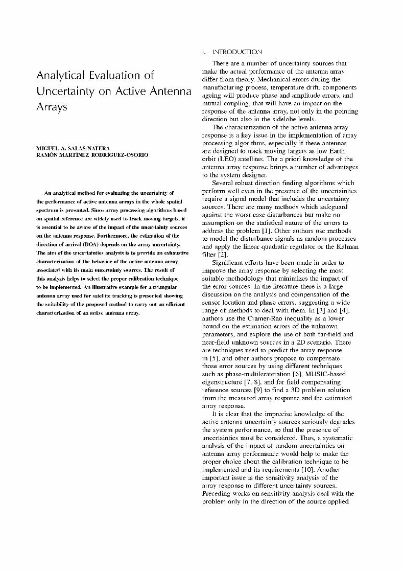
I. INTRODUCTION

Analytical Evaluation of Uncertainty on Active Antenna Arrays

MIGUEL A. SALAS-NATERA RAMÓN MARTÍNEZ RODRÍGUEZ-OSORIO

An analytical method for evaluating the uncertainty of

the performance of active antenna arrays in the whole spatial

spectrum is presented. Since array processing algorithms based

on spatial reference are widely used to track moving targets, it

is essential to be aware of the impact of the uncertainty sources

on the antenna response. Furthermore, the estimation of the

direction of arrival (DOA) depends on the array uncertainty.

The aim of the uncertainties analysis is to provide an exhaustive

characterization of the behavior of the active antenna array

associated with its main uncertainty sources. The result of

this analysis helps to select the proper calibration technique

to be implemented. An illustrative example for a triangular

antenna array used for satellite tracking is presented showing

the suitability of the proposed method to carry out an efficient

characterization of an active antenna array.

There are a number of uncertainty sources that make the actual performance of the antenna array differ from theory. Mechanical errors during the manufacturing process, temperature drift, components ageing will produce phase and amplitude errors, and mutual coupling, that will have an impact on the response of the antenna array, not only in the pointing direction but also in the sidelobe levels.

The characterization of the active antenna array response is a key issue in the implementation of array processing algorithms, especially if these antennas are designed to track moving targets as low Earth orbit (LEO) satellites. The a priori knowledge of the antenna array response brings a number of advantages to the system designer.

Several robust direction finding algorithms which perform well even in the presence of the uncertainties require a signal model that includes the uncertainty sources. There are many methods which safeguard against the worst case disturbances but make no assumption on the statistical nature of the errors to address the problem [1]. Other authors use methods to model the disturbance signals as random processes and apply the linear quadratic regulator or the Kalman filter [2].

Significant efforts have been made in order to improve the array response by selecting the most suitable methodology that minimizes the impact of the error sources. In the literature there is a large discussion on the analysis and compensation of the sensor location and phase errors, suggesting a wide range of methods to deal with them. In [3] and [4], authors use the Cramer-Rao inequality as a lower bound on the estimation errors of the unknown parameters, and explore the use of both far-field and near-field unknown sources in a 2D scenario. There are techniques used to predict the array response in [5], and other authors propose to compensate those error sources by using different techniques such as phase-multilerateration [6], MUSIC-based eigenstructure [7, 8], and far field compensating reference sources [9] to find a 3D problem solution from the measured array response and the estimated array response.

It is clear that the imprecise knowledge of the active antenna uncertainty sources seriously degrades the system performance, so that the presence of uncertainties must be considered. Thus, a systematic analysis of the impact of random uncertainties on antenna array performance would help to make the proper choice about the calibration technique to be implemented and its requirements [10]. Another important issue is the sensitivity analysis of the array response to different uncertainty sources. Preceding works on sensitivity analysis deal with the problem only in the direction of the source applied

System specification

^

System design

0 Analytical Uncertainties Evaluation and Report of uncertainties evaluation

I Specify the tolerance of

the active antenna components

Evaluate the uncertainty in the array response in a given pointing direction

Estimate the complete array response pattern

Choose the proper calibration technique

Implementation and Manufacturing

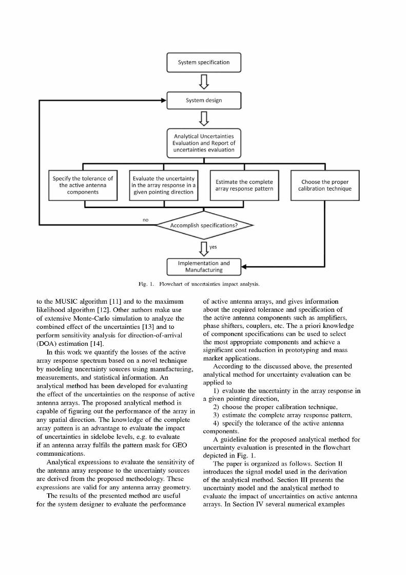
Fig. 1. Flowchart of uncertainties impact analysis.

to the MUSIC algorithm [11] and to the maximum likelihood algorithm [12]. Other authors make use of extensive Monte-Carlo simulation to analyze the combined effect of the uncertainties [13] and to perform sensitivity analysis for direction-of-arrival (DOA) estimation [14].

In this work we quantify the losses of the active array response spectrum based on a novel technique by modeling uncertainty sources using manufacturing, measurements, and statistical information. An analytical method has been developed for evaluating the effect of the uncertainties on the response of active antenna arrays. The proposed analytical method is capable of figuring out the performance of the array in any spatial direction. The knowledge of the complete array pattern is an advantage to evaluate the impact of uncertainties in sidelobe levels, e.g. to evaluate if an antenna array fulfils the pattern mask for GEO communications.

Analytical expressions to evaluate the sensitivity of the antenna array response to the uncertainty sources are derived from the proposed methodology. These expressions are valid for any antenna array geometry.

The results of the presented method are useful for the system designer to evaluate the performance

of active antenna arrays, and gives information about the required tolerance and specification of the active antenna components such as amplifiers, phase shifters, couplers, etc. The a priori knowledge of component specifications can be used to select the most appropriate components and achieve a significant cost reduction in prototyping and mass market applications.

According to the discussed above, the presented analytical method for uncertainty evaluation can be applied to

1) evaluate the uncertainty in the array response in a given pointing direction,

2) choose the proper calibration technique, 3) estimate the complete array response pattern, 4) specify the tolerance of the active antenna

components. A guideline for the proposed analytical method for

uncertainty evaluation is presented in the flowchart depicted in Fig. 1.

The paper is organized as follows. Section II introduces the signal model used in the derivation of the analytical method. Section III presents the uncertainty model and the analytical method to evaluate the impact of uncertainties on active antenna arrays. In Section IV several numerical examples

are exposed to clarify the applications and show the advantages of the proposed analytical evaluation method. Finally, Section V draws the conclusions of this paper.

II. SIGNAL MODEL

In order to expand the analytical method some assumptions must be imposed. Since this work is focused on the analysis of a generic active array, the problem has a 3-dimensional formulation and also assumes the validity of the narrowband approximation and the fact that the number of sensors is higher than the number of sources.

In the scenario under study, we consider an uncalibrated array of M antenna elements in the presence of N narrowband signals, and N < M. As an extension to the model proposed in [15] the array output signal vector x{t) can be expressed as

x(t) = CGoAs_(t) + n(t) (1)

where 0 represents the Hadamard product, C is an M xM matrix that represents the mutual coupling matrix, s(t) is the N x 1 vector of impinging signals, and «(f) is the M x l vector of uncorrected additive white Gaussian noise sources.

G is an M x N matrix whose nth column represents the gain g and phase <f> of the array elements in the direction of the nth source (0n,pn) as g(6n, ipn)e>^(9'"'Pn). Matrix A in (1) is an M x N matrix whose nth column an represents the ideal steering vector of the array in the direction of the nth source as fln = e^^l7TlX)rr", where r is the array location matrix, r'n is the unitary direction vector of the nth source, r'n = [(sm6ncospn sm6n&mpn cosi/?n)]

r, and A is the wavelength.

In order to include uncertainty errors, (1) can be rewritten as

x(t) = C(G + AG) © (A + AA) • s(t) + n(f) (2)

where AG and AA are M xM matrices that represent the array gain and phase uncertainty matrix and the sensor location uncertainty matrix, respectively. This model can be extended to include the impact of RF uncertainty sources in the M array branches due to the presence of analog components such as amplifiers, phase shifters, etc., as

x(t) = CiGjx + AGRF)(G + AG) © (A + AA) • s(t) + n(t)

(3) where Gpp, Gpp are a M xM diagonal matrices whose complex elements represent the gain of the RF circuit and the effect of the gain and phase uncertainty sources due to the active antenna array components.

The aim of the uncertainties analysis is to provide a complete characterization of the active antenna array

response associated with its main uncertainty sources in any spatial direction (0, p).

In general the array manifold of the array in the direction (0, p) can be obtained expressing G and A as M x 1 vectors representing the ideal pattern of the array elements and the ideal steering vectors, respectively, with AG and AA being their deviations due to the presence of uncertainties. The array manifold M_{0, p) can be expressed as

M(6, p) = CiGxr + AGRF)(G((?, p) + AG(6, p))

O(A(0,p) + AA(0,p)). (4)

Finally, the beamformed array pattern can be written in the presence of the uncertainty sources as

W,p)=WHM(0,p) (5)

where W_ is an M x 1 vector whose mth term represents the complex beamforming weight for the mth antenna element and ( ) H is the Hermitian operator. W_ is calculated to synthesize an antenna pattern that satisfies an optimization criterion, such as tracking of moving targets, cancellation of interference sources, etc. In the case of beamsteering to a specified target in direction (0, p), W_ can be expressed as

W = exp[-j(2ir/X)f?'n(0, p) - f_(0, p) - A ^ ^ ]

(6)

where Ai/> represents the phase deviation vector in the array branches due to the active and phase shifter components.

In the case where no errors due to uncertainties are present, the expression for the ideal beamformed array pattern Yo(0,p), can be rewritten as

Y0(6, p) = WZiCGjcpGiB, p) © A(6, </>))

= W_HoMo(0,p). (7)

III. ANALYTICAL MODEL FOR UNCERTAINTY EVALUATION

In this section we formulate the uncertainty problem about the difference of the expected (ideal) array pattern response and the array pattern response with uncertainty sources. We start with the theoretical formulation for the uncertainty sources and its influences on the measured or modeled output quantity of the antenna array under evaluation. The output quantity Y is related to the measurement result y through its combined standard uncertainty uc(y) with a confidence interval as [16]

Y=y±uc(y). (8)

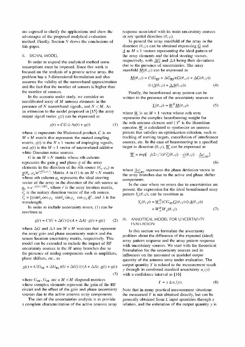
Note that in many practical measurement situations the measurand Y is not obtained directly, but can be generally obtained from L input quantities through a relation, and the estimation of the output quantity y is

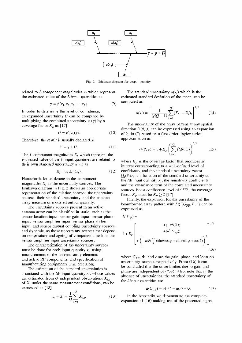
Fig. 2. Ishíkawa diagram for output quantity.

related to L component magnitudes x¡ which represent the estimated value of the L input quantities as

y =f(xvx2,x3,...,xL). (9)

In order to determine the level of confidence, an expanded uncertainty U can be computed by multiplying the combined uncertainty uc(y) by a coverage factor K as [17]

U = Kpuc(y). (10)

Therefore, the result is usually declared as

Y = y±U. (11)

The L component magnitudes X¡ which represent the estimated value of the L input quantities are related to their own standard uncertainty u(x¡) as

X¡ = x¡ ázu(x¡). (12)

Henceforth, let us denote to the component magnitudes Xl as the uncertainty sources. The Ishikawa diagram in Fig. 2 shows an appropriate representation of the relation between the uncertainty sources, their standard uncertainty, and the antenna array measure or modeled output quantity.

The uncertainty sources present in an active antenna array can be classified in static, such as the sensor location input, sensor gain input, sensor phase input, sensor amplifier input, sensor phase shifter input, and sensor mutual coupling uncertainty sources, and dynamic, as those uncertainty sources that depend on temperature and ageing of components such as the sensor amplifier input uncertainty sources.

The characterization of the uncertainty sources must be done for each input quantity x¡, using measurements of the antenna array elements and active RF components, and specification of manufacturing equipments (e.g. precision).

The estimation of the standard uncertainties is associated with the /th input quantity x¡, whose values are estimated from Q independent observations X¡ k

of Xl under the same measurement conditions, can be expressed as [18]

Q

X, 0z2xijc-^ k=\

(13)

The standard uncertainty u(x¡) which is the estimated standard deviation of the mean, can be computed as

u(x¡) = G(G-i) k=\

(14)

The uncertainty of the array pattern at any spatial direction U(6, ip) can be expressed using an expansion of Y0 in (7) based on a first-order Taylor series approximation as

U(8,ip)=l+Kp[J2Ql(6,ip) j = \

1/2

(15)

where KP is the coverage factor that produces an interval corresponding to a well-defined level of confidence, and the standard uncertainty vector Q_i(0,(p) is a function of the standard uncertainty of the /th input quantity x¡, the sensitivity coefficients, and the covariance term of the correlated uncertainty sources. For a confidence level of 95%, the coverage factor KP must be KP > 2 [17].

Finally, the expansion for the uncertainty of the beamformed array pattern with / G {Gpp,^ ,r} can be expressed as

u(e,<p)

l + KD

+ ( - « 2 ( * ) )

+ («2(GRF))

2TT -u(r) — (sm9 cosip + sine* sinip + cosí?)

1/2

(16)

where Gpp, Í*, and r are the gain, phase, and location uncertainty sources, respectively. From (16) it can be concluded that the uncertainties due to gain and phase are independent of (0, ip). Also, note that in the absence of uncertainties, the standard uncertainty of the / input quantities are

w(GRF) = «(*) = u(F) = 0. (17)

In the Appendix we demonstrate the complete expansion of (16) making use of the presented signal

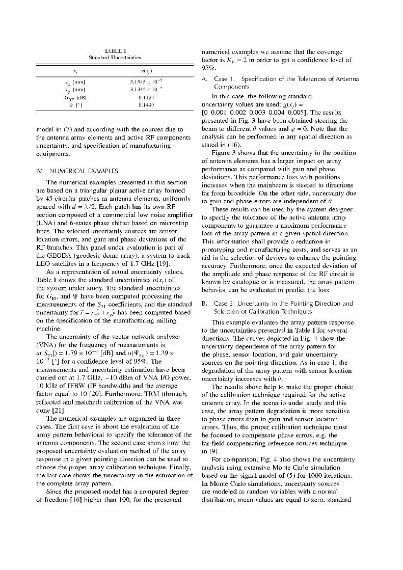
TABLE I Standard Uncertainties

xl

rx [mm] ry [mm]

GRF [dB]

* [°]

u{x¡)

3.1345 x 1(T5

3.1345 x 10~5

0.1121

0.1497

model in (7) and according with the sources due to the antenna array elements and active RF components uncertainty, and specification of manufacturing equipments.

IV. NUMERICAL EXAMPLES

The numerical examples presented in this section are based on a triangular planar active array formed by 45 circular patches as antenna elements, uniformly spaced with d = A/2. Each patch has its own RF section composed of a commercial low noise amplifier (LNA) and 6-states phase shifter based on microstrip lines. The selected uncertainty sources are sensor location errors, and gain and phase deviations of the RF branches. This panel under evaluation is part of the GEODA (geodesic dome array), a system to track LEO satellites in a frequency of 1.7 GHz [19].

As a representation of actual uncertainty values, Table I shows the standard uncertainties u(x¡) of the system under study. The standard uncertainties for Gjjp and Í* have been computed processing the measurements of the 521 coefficients, and the standard uncertainty for r = rxx + r y has been computed based on the specification of the manufacturing milling machine.

The uncertainty of the vector network analyzer (VNA) for the frequency of measurements is w(|S21|) = 1.79 x 10-4 [dB] and u(^sJ = 1.39 x 10~3 [°] for a confidence level of 95%. The measurements and uncertainty estimation have been carried out at 1.7 GHz, - 1 0 dBm of VNA I/O power, 10 kHz of IFBW (IF bandwidth) and the average factor equal to 10 [20]. Furthermore, TRM (through, reflected and matched) calibration of the VNA was done [21].

The numerical examples are organized in three cases. The first case is about the evaluation of the array pattern behavioral to specify the tolerance of the antenna components. The second case shows how the proposed uncertainty evaluation method of the array response in a given pointing direction can be used to choose the proper array calibration technique. Finally, the last case shows the uncertainty in the estimation of the complete array pattern.

Since the proposed model has a computed degree of freedom [16] higher than 100, for the presented

numerical examples we assume that the coverage factor is KP = 2 in order to get a confidence level of 95%.

A. Case 1. Specification of the Tolerances of Antenna Components

In this case, the following standard uncertainty values are used: w(x;) = [0 0.001 0.002 0.003 0.004 0.005]. The results presented in Fig. 3 have been obtained steering the beam to different 0 values and ip = 0. Note that the analysis can be performed in any spatial direction as stated in (16).

Figure 3 shows that the uncertainty in the position of antenna elements has a larger impact on array performance as compared with gain and phase deviations. This performance loss with positions increases when the mainbeam is steered to directions far from broadside. On the other side, uncertainty due to gain and phase errors are independent of 0.

These results can be used by the system designer to specify the tolerance of the active antenna array components to guarantee a maximum performance loss of the array pattern in a given spatial direction. This information shall provide a reduction in prototyping and manufacturing costs, and serves as an aid in the selection of devices to enhance the pointing accuracy. Furthermore, once the expected deviation of the amplitude and phase response of the RF circuit is known by catalogue or is measured, the array pattern behavior can be evaluated to predict the loss.

B. Case 2: Uncertainty in the Pointing Direction and Selection of Calibration Techniques

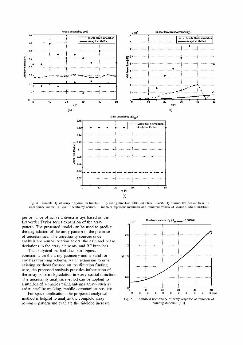
This example evaluates the array pattern response to the uncertainties presented in Table I for several directions. The curves depicted in Fig. 4 show the uncertainty dependence of the array pattern for the phase, sensor location, and gain uncertainty sources on the pointing direction. As in case 1, the degradation of the array pattern with sensor location uncertainty increases with 0.

The results above help to make the proper choice of the calibration technique required for the active antenna array. In the scenario under study and this case, the array pattern degradation is more sensitive to phase errors than to gain and sensor location errors. Thus, the proper calibration technique must be focused to compensate phase errors, e.g. the far-field compensating reference sources technique in [9].

For comparison, Fig. 4 also shows the uncertainty analysis using extensive Monte Carlo simulation based on the signal model of (5) for 1000 iterations. In Monte Carlo simulations, uncertainty sources are modeled as random variables with a normal distribution, mean values are equal to zero, standard

1.2

1

0 3

as

0.2

XJO^ Phase uncertainty u;1}')

u|l!')=O.0O5

1

üTO-ffiüM

; : J

u I1! '1=0.003

u ('!')= 0.002

UH')=0.001 u!-n-u

Sensor location uncertainty u(r)

20 30

on (a)

1.Z

1

0.8

0.6

ft 4

0.2

xio"1 Gain

1

uncertainty "í<V • 1

u(al=0,005

•i

u(a)=0.0O4

-

ula)=0.003

u(a)=0.002

u(q)=0.00l uflhU

4'J 50 0 10 20 30

en (c)

Fig. 3. Uncertainty [dB]. (a) Phase uncertainty source, (b) Sensor location uncertainty source, (c) Gain uncertainty source.

deviation in Table I, and initialized with a new seed per iteration. It can be seen that the results using the analytical formulation lie in the valid confidence interval given by the Monte Carlo simulation. Therefore, the proposed analytical method offers a significant reduction in computational complexity and time as compared with Monte Carlo using (16). To contrast uncertainty results to Monte Carlo simulations properly, the coverage factor is assumed KP = 1 in the separated uncertainty source simulations in Fig. 4.

The curve depicted in Fig. 5 shows the uncertainty dependence of the array pattern for the phase, sensor location, and gain as combined uncertainty on the pointing direction using uncertainty sources in Table I and (29). As explained in Section III, for a confidence level of 95% the coverage factor is assumed to be KP = 2. Due to the precision of the figure, the total uncertainty in Fig. 5 for this simulation is 0.56876 dB plus the curve values as f/combined = curve values + 0.56876 dB.

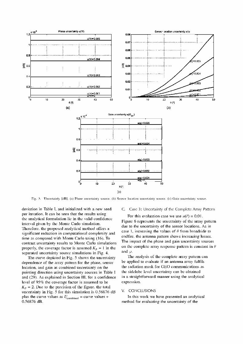
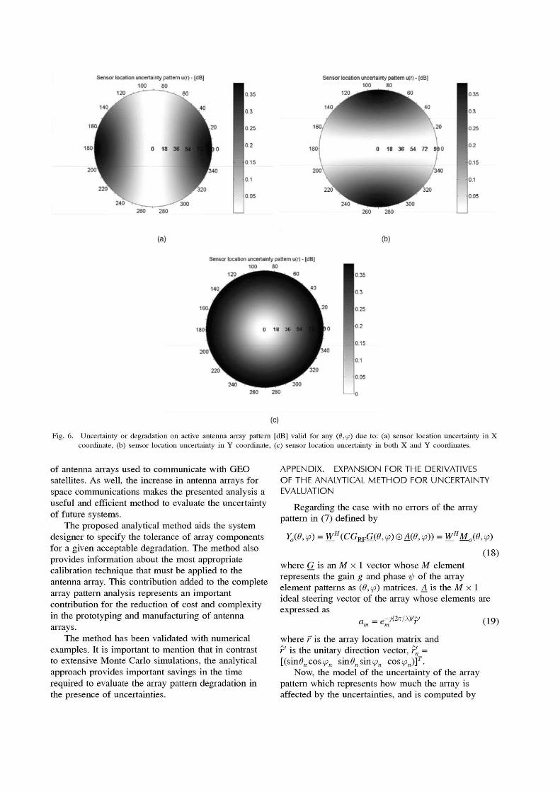
C. Case 3: Uncertainty of the Complete Array Pattern

For this evaluation case we use u(r) = 0.01. Figure 6 represents the uncertainty of the array pattern due to the uncertainty of the sensor locations. As in case 1, increasing the values of 0 from broadside to endfire, the antenna pattern shows increasing losses. The impact of the phase and gain uncertainty sources on the complete array response pattern is constant in 0 and (p.

The analysis of the complete array pattern can be applied to evaluate if an antenna array fulfils the radiation mask for GEO communications as the sidelobe level uncertainty can be obtained in a straightforward manner using the analytical expression.

V. CONCLUSIONS

In this work we have presented an analytical method for evaluating the uncertainty of the

Phase uncertainty u^H')

OG

0.5

0 1

0.3

0.2

0.1 •

0

-0.1

*

Monte Carlo simulation ^ — Analytical Method

• + * • ;

+ + + -*—i

* +

-> '

S

8

7

1 = 3

:'

1

n

^ inJ& Sensor location uncertainty u(rj

• — • - • Monte Cario simulation ^—^— Analytical Method

+

i

*

•

* - ¡.....,»>'

1 i • T " "i • ••»• T ~ — 1 1 1 £ ' 10 20 30

en (a)

4Í1 no

Gain uncertainty u(GRJ

10 20 30

(b)

40 SO

Fig. 4. Uncertainty of array response as function of pointing direction [dB]. (a) Phase uncertainty source, (b) Sensor location uncertainty source, (c) Gain uncertainty source. + markers represent maximun and minimun values of Monte Carlo simulation.

performance of active antenna arrays based on the first-order Taylor series expansion of the array pattern. The presented model can be used to predict the degradation of the array pattern in the presence of uncertainties. The uncertainty sources under analysis are sensor location errors, the gain and phase deviations in the array elements, and RF branches.

The analytical method does not impose constraints on the array geometry and is valid for any beamforming scheme. As an extension to other existing methods focused on the direction finding case, the proposed analysis provides information of the array pattern degradation in every spatial direction. The uncertainty analysis method can be applied to a number of scenarios using antenna arrays such as radar, satellite tracking, mobile communications, etc.

For space applications the proposed analytical method is helpful to analyze the complete array response pattern and evaluate the sidelobe increase

2.5-

2 -

Combined uncertainty (U - 0.56876)

Fig. 5.

10 20 0

30 0

40 0

50 0 U)

Combined uncertainty of array response as function of pointing direction [dB].

Sensor location uncertainty pattern u:r; • [d3l

100 SO

t 40

Y°

n spo

/340

r320

0 35

l o 3

lo.2S

Hu2

I0.15

0.1

0.05

(a) (b)

Sensor location uncertainty pattern u<r) - |dBJ

100 60

120^

(C)

Fig. 6. Uncertainty or degradation on active antenna array pattern [dB] valid for any (6,<p) due to: (a) sensor location uncertainty in X coordinate, (b) sensor location uncertainty in Y coordinate, (c) sensor location uncertainty in both X and Y coordinates.

of antenna arrays used to communicate with GEO satellites. As well, the increase in antenna arrays for space communications makes the presented analysis a useful and efficient method to evaluate the uncertainty of future systems.

The proposed analytical method aids the system designer to specify the tolerance of array components for a given acceptable degradation. The method also provides information about the most appropriate calibration technique that must be applied to the antenna array. This contribution added to the complete array pattern analysis represents an important contribution for the reduction of cost and complexity in the prototyping and manufacturing of antenna arrays.

The method has been validated with numerical examples. It is important to mention that in contrast to extensive Monte Carlo simulations, the analytical approach provides important savings in the time required to evaluate the array pattern degradation in the presence of uncertainties.

APPENDIX. EXPANSION FOR THE DERIVATIVES OF THE ANALYTICAL METHOD FOR UNCERTAINTY EVALUATION

Regarding the case with no errors of the array pattern in (7) defined by

Yo(0,(p) = WH(CGKFG(6,v)®A(6,v)) = WHM^(.d,<p)

(18) where G is an M x 1 vector whose M element represents the gain g and phase %jj of the array element patterns as (6,(p) matrices. A is the M x\ ideal steering vector of the array whose elements are expressed as

a = e-ji27r'x)rr'

m m

where f is the array location matrix and r' is the unitary direction vector, r'n = [(sin#„cos(/5„ sin0nsin<¿>n cos^)] 1 ' .

Now, the model of the uncertainty of the array pattern which represents how much the array is affected by the uncertainties, and is computed by

(19)

the expansion of a first-order Taylor series of Y0 to evaluate the uncertainty of the array at any spatial direction U(6,(p), was defined in (15) as

U(0,íp) = í+Kp[Y,íli(0,'P) a=\

1/2

(20)

where KP is the coverage factor and the standard uncertainty vector Q_i(9,(p) is a measure of the correlation between the array response and the uncertainty sources based on the standard uncertainty u{xj) of the /th input quantity x¡, the sensitivity coefficients, and the covariance term of the correlated uncertainty sources. The standard uncertainty vector can be expressed as

OK^)=(g^))2 + 2(mj-)^,^).

(21)

The partial derivatives dY0/dxl are the partial derivatives with respect to the component magnitudes Xl evaluated at Xl = x¡. Note that when there are correlated input quantities as x¡ and xl+l, it must be computed as the second term of the equation above which denotes the correlated uncertainty associated to the correlation coefficient as

u(x¡,xl+l) = u(xi)u(xi+iy(x¡,Xi+l). (22)

The correlation coefficient is a measure of the dependency between x¡ and xl+l, where r(x¡,xl+l) = r(xl+l,x¡) and — 1 < r(xl+l,x¡) < 1. If there are uncorrected input quantities x¡ and xl+l, r(xl+l,x¡) = 0 [17, 22].

From now on let us center the attention on those uncertainty sources due to the antenna array elements and active RF components uncertainty, and specification of manufacturing equipments; the partial derivatives with respect to the component magnitudes should be those with respect to Gj p, Í*, and r, denoted in Section II as the gain, phase, and location uncertainty sources, respectively.

The expression to evaluate the sensitivity of the array pattern to the phase uncertainties can be obtained by the partial derivative of Y0 with respect to <J as

dY dWH

Q£(6,<P) = - ^ - ( C G R F G ^ O A ^ ) ) (23)

BY Q£(6,<P) = (-J)WH(CGKFG(e,v)QA(e,v)).

(24)

Similarly, the gain uncertainties from the RF circuit, array elements, and components can be evaluated as gain errors in the array pattern by the derivative of Y0 with respect to Gj p, and the array pattern Y0 depends on Gpp through M_o{0,ip). Thus,

the expression for the derivative of Y0 with respect to ie w

dYn

Gjjp can be written as

dG -(0,ip) = W_H{CQ{0,ip)(DA{0,ipy). (25)

RF

The sensor location uncertainties of the array elements can be evaluated by the derivative of Y0 with respect to r and expressed by

BY 0^(0, </>) = (-JKr')WH(CGKFG(6,v)QA(6,v))

(26)

where r' is the sum of the unitary direction vector terms as

-' = £?v (27) v = l

Finally, the standard uncertainty vector 0^(0, y>) with / G {Gjjp,^,^} can be expressed as

2

0(0, (f) Y}

5 * (0,</>M*)

dY M ^ M S R F ) RF dG ^

dY H6,<P>(ñ

df

In decibels representation can be written as

f/dB(0,(/5) = 2Ologlot/(0,(/>).

REFERENCES

(28)

(29)

[1] Ratnarajah, T. and Manikas, A. An H-inf approach to mitigate the effects of array

uncertainties on the MuSIC algorithm. IEEE Signal Processing Letters, 5, 7 (July 1998).

185-188. [2] Pierre, J. and Kavech, M.

Experimental performance of calibration and

direction-finding algorithm. In Proceedings of the IEEE International Conference on Acoustics, Speech, and Signal Processing, Toronto, 1991,

pp. 1365-1368. [3] Rockah, Y. and Schultheiss, P.

Array shape calibration using sources in unknown

location—Part I: Far field sources. IEEE Transactions on Acoustic, Speech and Signal Processing, 35, 3 (Mar. 1987), 245-253 .

[4] Rockah, Y. and Schultheiss, P.

Array shape calibration using sources in unknown location—Part II: Near field sources and estimator

implementation. IEEE Transactions on Acoustic, Speech and Signal Processing, 35, 6 (June 1987), 286-299 .

[5] Gupta, I. J., et al.

An experimental study of antenna array calibration.

IEEE Transactions on Antennas and Propagation, 51 , 3 (Mar. 2003), 664-667 .

[6] Lee, E. and Dorny, C. N.

A broadcast reference technique for self-calibration of large antenna phased array.

IEEE Transactions on Antennas and Propagation, 37, 8 (Aug. 1989), 534-544 .

[7] Weiss, A. J. and Friedlander, B.

Array shape calibration using eigenstructure methods. In Proceedings of the Twenty-Third Asilomar Conference

on Signals, Systems and Computers, vol. 2, Pacific Grove,

CA, Nov. 1989, pp. 925-929 . [8] Friedlander, B. and Weiss, A. J.

Eigenstructure methods for direction finding with sensor gain and phase uncertainties. In Proceedings of the IEEE International Conference on

Acoustics, Speech, and Signal Processing, vol. 5, New York, Apr. 1988, pp. 2681-2684.

[9] Weijun, Y., Yuanxun, W , and Itoh, T.

A self-calibration antenna array system with moving apertures.

In IEEE MTT-S International Microwave Symposium Digest, vol. 3, Philadelphia, June 2003, pp. 1541-1544.

[10] Borat, B. and Friedlander, B.

Accuracy requirements in off-line array calibration. IEEE Transactions on Aerospace and Electronic Systems, 33, 2 (Apr. 1997), 545-556 .

[11] Friedlander, B.

A sensitivity analysis of the MUSIC algorithm. IEEE Transactions on Acoustics, Speech and Signal

Processing, 38, 10 (Oct. 1990), 1740-1754. [12] Friedlander, B.

Sensitivity analysis of the maximum likelihood

direction-finding algorithm. IEEE Transactions on Aerospace and Electronic Systems, 26 (Nov. 1990), 953-968 .

[13] Collado, A., et al.

Combined analysis of systematic and random uncertainties for different noise-figure characterization

methodologies. In IEEE MTT-S International Microwave Symposium

Digest, Philadelphia, June 2003, pp. 1419-1422. [14] Aliyazicioglu, Z., et al.

Sensitivity analysis for direction of arrival estimation

using a Root-MUSIC algorithm. In Proceedings of the International MultiConference of

Engineers and Computer Scientists, vol. 2, Hong Kong, China, Mar. 2008.

[15] Mowler, M., et al.

Joint estimation of mutual coupling, element factor, and phase center of antenna arrays. EURASIP Journal on Wireless Communications and

Networking, 2007, 2 (Jan. 2007). [16] Taylor, B. N. and Kuyatt, C. E.

Guidelines for evaluating and expressing the uncertainty of NIST measurement results. National Institute of Standards and Technology, NIST

Technical Note 1297, 1994. [17] International Organization for Standardization

Guide to the Expression of Uncertainty in Measurement.

International Organization for Standardization, ISO/IEC Guide 98:1993, 1993.

[18] Box, G., Hunter, W., and Hunter, J. S.

Statistics for Experimenters. New York: Wiley, 1980.

[19] Sierra-Perez, M., et al.

GEODA: Adaptive antenna array for Metop satellite signal reception.

In Proceedings of the 4th ESA International Workshop on Tracking, Telemetry and Command System for Space Application, Darmstadt, Germany, Sept. 2007, pp. 1-4.

[20] Bednorz, T.

Measurement uncertainties for vector network analysis. Rohde & Schwarz Application Note 1EZ29.1E, Oct.,

1996. [21] Krekels, H-G.

Automatic calibration of vector network analyzer ZVR.

Rohde & Schwarz Application Note 1 E Z 3 0 ^ E , May, 1998.

[22] Dietrich, C. F.

Uncertainty, Calibration and Probability (2nd ed.). Bristol, UK: Adam Hilger, 1991.

Miguel Alejandro Salas-Natera was born in Valencia, Venezuela, in 1979. He received the electrical engineer degree and the management diploma, both, from the Universidad de Carabobo, Valencia, Venezuela, in 2003 and 2004, respectively. He has worked as a technical project assessor in KVI Inversions in 2003. He participated in the implementation of the logistic system for distribution in AMBEV in 2004, and in 2005, he worked at DIGITEL TIM as a services manager.

He received the Ph.D. degree in signal, system and radiocommunications and a masters degree in space technologies, both from the Technical University of Madrid, Madrid, Spain in 2011. His research areas are smart antennas performance in satellite communications, digital receivers for ground stations that make use of antenna arrays, and measurement, characterization, and calibration of antenna arrays.

Ramón Martínez Rodríguez-Osorio was born in Madrid, Spain, in 1975. He received the Ingeniero de Telecomunicación and the Doctor Ingeniero de Telecomunicación degrees in 1999 and 2004 from the Universidad Politécnica de Madrid (UPM).

In 1999, he joined the Departamento de Señales, Sistemas y Radiocomunicaciones of the E.T.S.I. de Telecomunicación at Universidad Politécnica de Madrid, where he currently works as associate professor. His main research areas are smart antennas arrays for mobile and satellite communication systems, satellite communications, and GNSS software receivers. He has participated in National and European projects (FP6, COST, ESA), and with private companies as researcher and as principal investigator. He is also responsible for nanosatellite activities in ETSIT-UPM, leading student projects related to ground stations and communications.

Professor Martinez received the Telefónica Móviles Prize for the Best Ph.D. Thesis in the area of UMTS in 2004 and is coauthor of three patents. He has published his research work at international conferences and in journals, and is coauthor of five book chapters. He is also the Academic Secretary of the Master in Space Technology Program (Universidad Politécnica de Madrid).