JOURNAL OF CHROMATOGRAPHY 25

THEORY OF PARTITION CHROMATOGRAPI-IY

II. NUMERICAL CALCULATIONS

Instit~atle of Physical Cheanislvy, Univevsily of Uppsala (Sweden)

(Rcccixcl hu,aust srcl, 1961)

The theoretical treatment of partition chromatography, advanced in an earlier articlel, has now been supplemented by numerical calculations performed on a digital computer. In the present calculations the treatment in ref. I has been closely followed and therefore only a short summary of the method is given here.

In the model used in the theory, the chromatographic column is divided into cells ‘of equal width and the operation of the column is assumed to take place in discontinuous steps. During a step the solution in the mobile phase of a cell is allowed to exchange solute with the stationary phase of that cell (lateral diffusion) and with solutions of the mobile phase in neighbouring cells (longitudinal diffusion). At the end of the step the solutions of the mobile phase in each cell are instantaneously shifted one step to the adjacent cells and the equilibration procedure is repeated. The solute concentration in the mobile phase of a particular cell is designated fg J, where i is the number of the cell and j the ,time (with the duration of a step being taken as the time unit). Thus fg 3 defines a matris where the ith row gives the solute concen- tration in the ith cell at different times and the jth column gives the distribution of the solute concentration in the mobile phase over the entire chromatographic column at the time j. The elements of the matrix fi 3 are calculated from the characteristic pctrameters ancl the initial conditions of the column operation according to Eqns. (23) and (24) in ref. 1. _ - In order to-simplify’the tfeatment the last term in Eqn. (24) is neglected, i.e. longitudinal diffusion in the statipnary phase is not taken into account. This ap- proximation is of minor significance for the theory, but it makes possible the use of a single recursion formula for the determination of ft I. It: takes the form:

where :

201 El =,-

tZJ2

p=__- YV2 *+VL VL + yv2 ( _ e - 1)11

YV2 >

YV2 ‘V = ---

Vl f YV2

(1 - (y”‘?)

26

with :

w. VINIC

The following parameters characterize the column operation :

VI, v, = volumes per interphase area of mobile and stationary phase respectively D,, D, = diffusion coeflicients in mobile and stationary phase respectively

Y = partition coefficient V = translational velocity of the mobile phase.

The initial conditions are given by the elements fO j and fi .j in Eqn, (I), and were in all cases chosen to represent a rectangular concentration peak in the solution entering the chrornatograpliic column.

The results were abstracted from the cornputor in the form of a few selected columns of a matris, representing the concentration distribution in the rnobi1.e phase of the chromatographic column at different times. For a detailed characterization of the distributions their zeroth, first and second moments, with respect to the origin and with the cell width as unit of length, were also calculated. For the jth column they are defined in the following way:

440 = c flj i (2)

(3)

(4)

It was found during the course cf tht: calculations that the zeroth moment A, (representing the amount of solute in the mobile phase) in a given matrix generally very rapidly converges to a constant value. Hence a normalization on a common basis of the distributions represented by the different matris columns is possible, The normalised distributions may then be characterized by the mean ,LC and the second moment around the mean ,u~. They are defined, as follows:

, I_& = A l/d4 (j (5)

p2 = A2/Ao --,I.$ (6)

In addition the mocle M, defined as the location 01 the masimum of the smoothed clistribution curve, was also determined.

Both ,U ancl ICI are measures of location of the distribution, whereas ,u2 is a measure of dispersion, Further, as a measure of skewness Pearson’s measure S is used. It is defined in the following way:

---A4 -_ s = /-I 3/].42

(7)

In the following the results will in general be given in terms of the parameters A,,, M, ,u, ,u2 and S.

l Here tile clepcnclcncc of IW. on the partition coef’f’lcicnt y is tnltcn cliffcrcnt from that in ref. I, It takes into account the assumption thak diffusion in the stationary phase is the rate clctcrmining step in lcltcral diffusion. It simply stabs that the volume term of the mobile phase (\vllerc the concentrstion is ltcpt uniform by convection) is changed in proportion to y,

THEORY OF PARTITION CHROMATOGRhFHY. II. 27

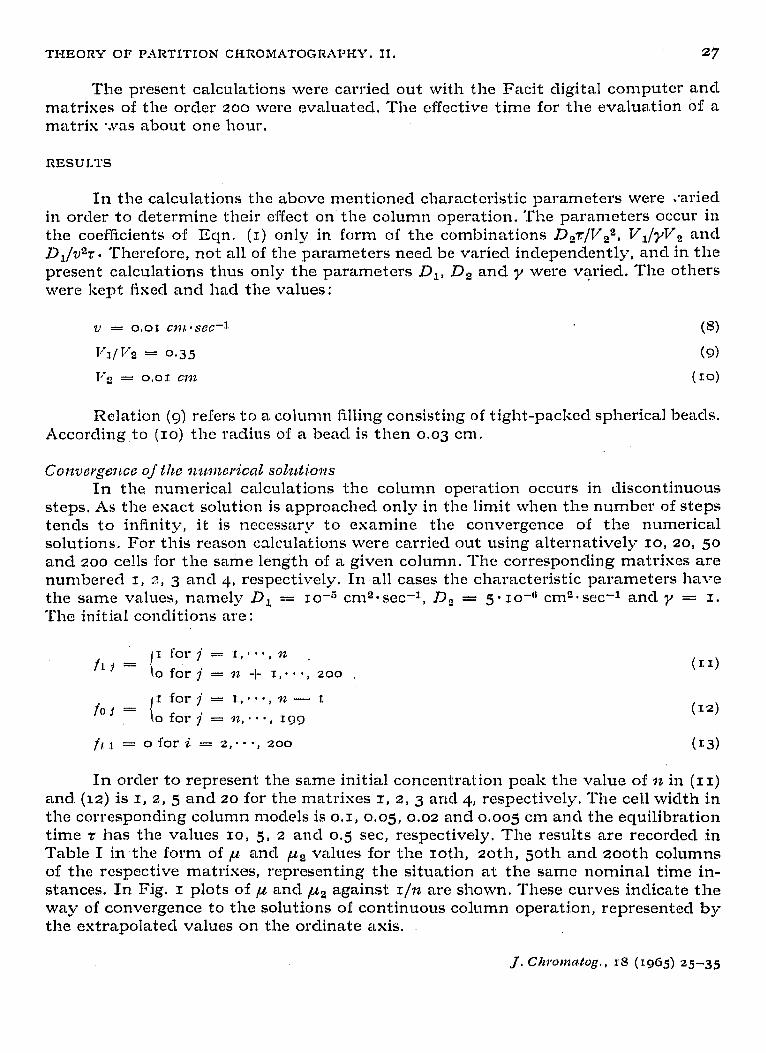
The present calculations were carried out with the Facit digital computer and matrixes of the order zoo were evaluated. The effective time for the evaluation of a matris *,vas about one hour.

RESUJ,TS

In the calculations the above mentioned characteristic parameters were :ariecl in order to determine their effect on the column operation. The parameters occur in the coeCcients of Eqn. (I) only in form of the combinations D,t/V,2, V,/yV2 ancl D,/v% l Therefore, not all of the parameters need be varied independently, and in the present calculations thus only the parameters D,, Da and y were vyied. The others were kept Axed and had the values:

v = 0.01 cm*sl?c-1 (8)

Relation (9) refers to a column filling consisting of tight-packed spherical beacls. According to (IO) the radius of a bead is then 0.03 cm.

In the numerical calculations the column operation occurs in discontinuous steps, As the esact solution is approached only in the limit when the number of steps tends to infinity, it is necessary to esamine the convergence of the numerical solutions. For this reason calculations were carried out using alternatively 10, 20, 50

and zoo cells for the same length of a given column. The corresponcling matrises are numbered I, R, 3 and 4, respectively. In all cases the characteristic parameters have the same values, namely D, = IO-~ cm2. set-1, D, = 5 - IO-(~ cm0 a set-l and y = I.

'The initial conditions are :

11 for j = I,***, 72

“’ = 10 for j

.

= 92 -1_ I,“‘, 200 (11)

(12)

fr I = 0 for i = z,*.*, 200 (13)

In. orcler to represent the same initial concentration peak the value of $2 in (II) and. (12) is I, 2, 5 and 20 for the matrises I, 2, 3 and 4, respectively. The cell width in the corresponding column models is 0.1, 0.05, 0.02 and 0.005 cm and the equilibration time t has the values IO, 5 , 2 and 0.5 set, respectively. The results are recorded in Table I in the form of ,U ancl ,u2 values for the Roth, moth, 50th ancl 200th columns of the respective matrises, representing the situation at the same nominal time in- stances. In Fig. I plots of p ancl p2 against I/U are shown. These curves indicate the way of convergence to the solutions of continuous column operaCon, represented by the extrapolatecl values on the ordinate asis.

2s

MhTRIX NUS. I, 2. 3 AND 4

CL 4.10% 3.4014 3.0495 a.gozS

PO I.G$gI I.211 1.037 I.006

The influence of both the lateral and longitudinal diffusion coefficients and the partition coefficient is established by separately changing these parameters. In all these calculations the value 72 = 5, in the initial conditions (II) and (IZ), is used and the value oft is 2 set giving a cell width of 0.02 cm. The conditions are then reasonably close to those of continuous column operation.

01 t I

0 0.5 I l/n

Pig. I. Convergence of solutions from discontinuous column operation.

In the matrixes numbered 5, G and 7 different longitudinal diffusion coefficients are used, D, having the values o, 10-6 and 5 0 IO-~ cm20 set-1, respectively. (The results are recorded in Table II.) In the matrises numbered S, g and IO, different lateral diffusion coefficients are used, the values of D, being co, IO-O and IO-’ cm2*sec-1, ‘respectively, (The results are recorded in Table III). To this group belongs also matrix No. 5 in Table II, for which D2 = 5 l 10-o cm2*sec- 1. Finally, in the group of matrixes numbered II, 12, 13, 14, 15 and 16 the partition coefficient is varied, the values of y being o, 0.1, 0.2, 0.5, 2 and 5, respectively. (The’results are shown in Table IV). To this group belongs also matrix No. 6 in Table II, for which y = I.

DISCUSSION

From the results in Tables II-IV it is seen that in all cases, except matrix No. IO,’ steady state conditions are established i n the chromatographic column. The steady state is characterized by constancy in the value of total solute concentration in the

J. ChvoWzatog., 18 (196.5) 25-35 . .

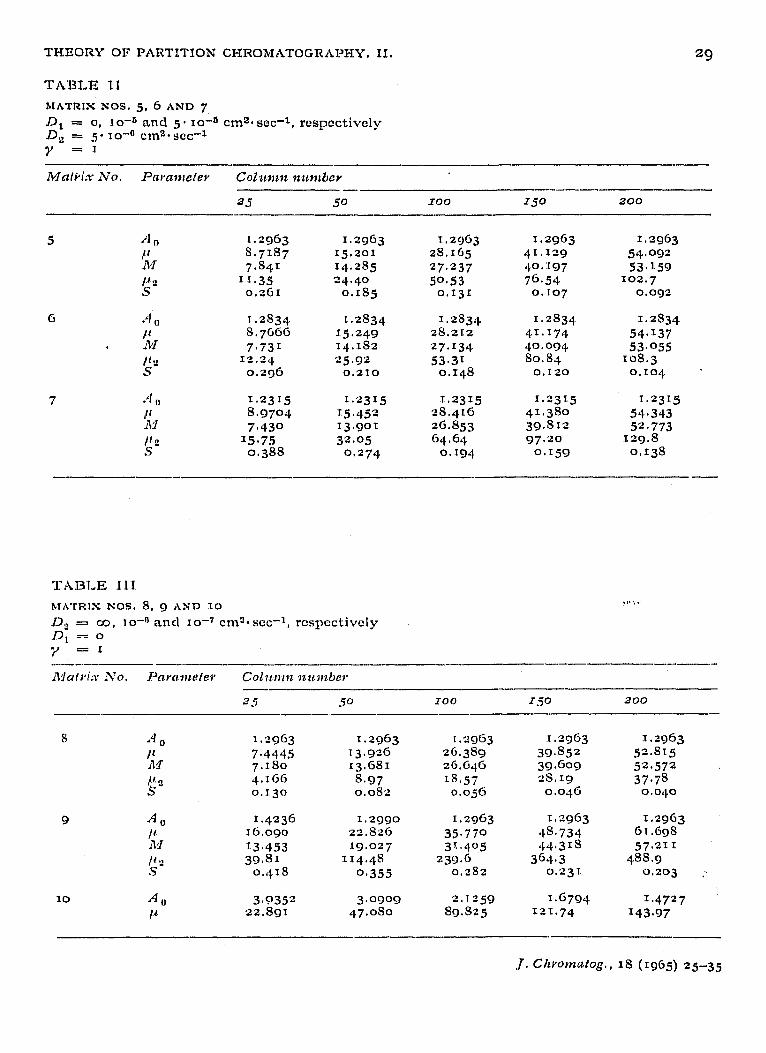
TI-IEORY OF PARTITION CHROMhTOGRRPI-IY. II. 29

MATRIS NOS. 5, G AND 7

131 = 0, IO-‘ and 5 * 10-s cm21 set-l, respcctivcly D, = 5. IO-” crn2.wz1

Y =I

MnlLi,v x0. Pwa7mfer cot?ac77~7a 7au77tber - a--

2.5 50 100 ISO 200

5 A" I.2903 I.2903 I.2963 I.2963 I.2963 I' 8.7137 15.201 25.165 41.12g 54,092 Iv 7.541 14.255 27.237 40.197 53,159 I! 02 II.35 24.40 50.53 76.54 102.7 s 0.2GI 0.155 0.131 0.107 0.092

G A 0 1.2S34 I.2834 1.2834 1.2S34 1.2S34

& 8.7066 15.249 2s.212 41.174 54*=37 7.731 I‘[.IS2 27.134 40.094 53.055

/In 12.24 25.92 53.31 So.84 108.3 s 0.296 0.210 O.I‘#S 0.120 0.104 .

7 )J o I.2315 I.2315 I.2315 X.2315 1.2315

I' 8.9704 15.452 25.416 41.3so 54.343 ATI 7,430 13.901 26.553 3g.s12 52,773 1'2 =5*75 32.05 64.64 97.20 12g.s s 0,3ss 0,274 0.194 0.159 0.13s

-..... ____

hIhTR1.S NOS. 8, 9 AND IO

12, = 03, 10-O nncl IO-’ cm2* ~cc-~, rcqxctivcly D, - 0 ‘J =I. --_.- --- - ---- iVct/ri;v No. Pnvtr7rretev coz~/t~rlzrt 7tzc~dJe,~

2 5 50 100 I.50 a00 --. ---- -_

8 A " 1.2gG3 1.2gG3 1.2gf.33 T ,2gG3 I. 2963

11 7.4445 13.920 2G.359 39.S52 52.SI5

M 7.1so r3.GS1 26.646 39.609 52.572 $2 4.rGG o.os2 S-97 18-57 2s,1g 37.75

0.130 0.05G 0,046 0.040

9 A" I.4236 1.2ggo 1.2963 I,2963 I.2963 1" IG.090 22.S2G 35.770 45.734 GI.Gg8 A!! 13.453 19.027 31.405 44031s 57.211

111 3g.Sr 114.48 239.0 304.3 485.9 s 0,418 0.355 0.2S2 0.231 0.203 ,

10 A0 309352 3.0909 2.T259 I.6794 I.4727 p 22,sgr 47.oso sg.s25 121.74 I43.97

J. Chrornalog., IS (1965) 25-35

30 H. VINK

BIATRIS Nos. II, 12. 13, 14, 15 AND I6

D, = IO-~ crn2*sc~-~ D, = 5'10 -0 cm2esec-1

Y = 0, 0.1, 0.2, 0~5, 2 and 5, rcspcctively

Matrix No. Parameter Cobacmn natntbev

2.5 50 100 I50 c! 200

II

15 A0 14.

M

!? 16 A0 0.32386 0.32386 0.3238G a3238G 0.3238G

P 3.5086 5.1442 8.4'54 Il.687 14,958 M 2.913 4.404 7.695 Io.gGG 14.228

Pi? I.874 3.717 7.403 11.10 14.78 s o-436 0.354 0.265 0.216 0.1go

4.9500 4.9500 4.9500 4.9500 23.071 48.071 98.071 148.071 22.950 48.oog 98.039 148.050

4.13 6.55 11.6 16.7

0.059 0.023 0.009 0.005

3.8540 3.8500 3.8500 3.8500 19.892 39.358 75.24.7 117.135 21.878 43.777 8~.422 120.212 x8.94 54.27

--b.Goo 125.8 197.1

-0.457 -0.283 -0.21g

3.1519 3.1500 3.1500 3,150o 3,1500

17.385 33.302 65.121 96.937 I 28.756 20.329 34.641: 66.309 98.087 129.887

23.72 62.37 139.6 217.3 294.3 -0.Go4 -0.170 --0.101 -0.078 -o.oGG

2.0383 2.0382 2.0382 2.0382 2.0382 12.581 22.875 43*4G3 G4.o.52 840G38 12.02G 22.234 42.790 G3.3GG 83.951 20.56 47.04 99.89 152.8 205.6 0.122 0.093 0.067 0.056 0.048

0.73724

:zl 51602

0.394

3*4GG4

3A48g 156.013

159.044 26707 -0.186

0.73724 0.73724 a.73724 0073724 9.4976 16.944 24.391 31.838

8.789 15.986 23.424 30.876 11.38 22.95 34.52 46.10 0.210 0.200 0.165 0.142

mobile (and stationary) phase of the chromatogra.phic column.This value is independ- ent of the diffusion coefficients D, and D2 and, for a column of given geometry, depends only on the partition coefficient y. The minor differences found in Tables II and III are due to end effects (diffusion out through the column ends). Under steady state conditions very simple rules esist concerning the translational velocity (peak velocity) and spreading of a concentration peak.

Peak velocity The absolute peak velocity may be defined as the translational velocity of the

center of mass of a concentration peak. A more convenient quantity is the relative

J. ChYOmatOg.. 18 (1965) 25-35

THEORY OF PARTITION CHROMATOGRAPWY. II. 31

peak velocity, which will be designated by Y and is defined as the ratio between the absolute peak velocity and the velocity of the mobile phase. It is obtained directly as the absolute velocity of the peak if the width of a cell and the equilibration time t are used as length and time units respectively, as then the velocity of the mobile phase becomes unity,

P

100

0 0 100 200 j

Fig. 2. Peak location as functions of time. Numbers in the matrix No, IO stcacly state is not established.

figure inclicstc matrix numbers . For

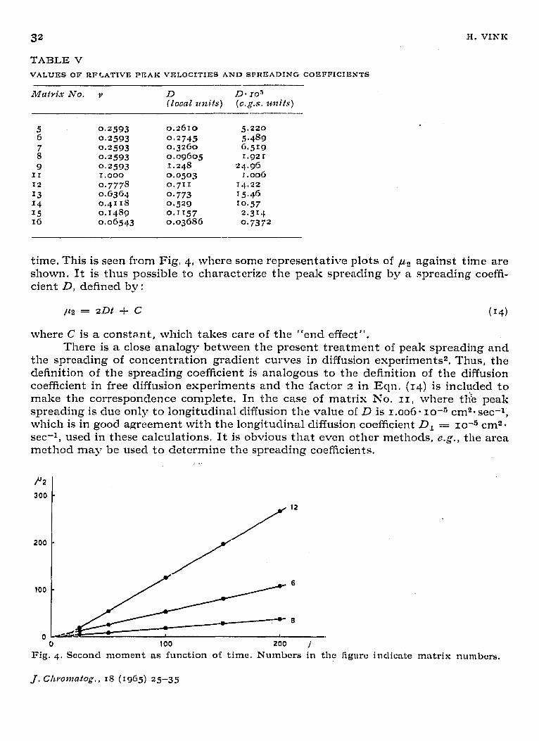
From the data in Tables II, III and IV it follows that under steady state conditions the peak velocity is constant. This is illustrated for some representative cases in Fig. 2, where plots of ~1 against time are shown, The calculated values of v are recorded in Table V. It is seen to be independent of the diffusion coeficients D, and Dz, but strongly dependent on the partition coefficient. The latter is illustrated in Fig. 3, where a plot of v against y is shown.

The breadth of a concentration peak is determined by its second moment around the mean p2. Under steady state conditions this is found to be a linear function of

0’ I 1 .--

0 1 2 Y Fig. 3. Peak velocity and spreading coefficient as fun&on of partition coefficient.

J. Cltromatog., ~8 (19%) 25-35

32

TABLE V

VALUES OF RFLATIVIZ PIZAIC VELOCITIES AND SPRl3ADING COEPPICIENTS

-

Ma&ix No. v D Da IOJ

(load zcnils) (c,g.s, znzils)

5 G

is

9 II

12

13 *4 I5 16

0.2593 0,2593 0.2593 o-2593 0.2593 1.000

0.777s 0.6364 0.4115 0.14sg o.oG543

0.2610

0.2745 0.3260 o.ogGo5 1.24s 0.0503 0.711

0.773 0.529 0.1157 o.o3GSG

5.220

5.459 G.519 I.921

2.t.96

r.ooG 14.22 15.46

IO.57 2.3r4 0.7372

time. This is seen from Fig. 4, where some representative plots of ,ue against time are shown. It is thus possible to charactcrize the peak spreading by a spreading coeffi- cient D, defined by:

p2 = 2.m + c (r4)

where C is a constant, which takes care of the “end effect”. There is a close analogy between the present treatment of peak spreading and

the spreading of concentration gradient curves in diffusion esperiment@. Thus, the definition of the spreading coeffkient is analogous to the definition of the diffusion coefficient in free diffusion esperiments and the factor 3 in Ecln. (14) is included to make the correspondence complete. In the case of matris No. II, where tlk peak spreading is due only to longitudinal diffusion the value of D is I.OOG* IO-~ cm2- set-1, which is in good agreement with the longitudinal diffusion coefficien.t D, = 10-5 cm29

set-f , used in these calculations. It is obvious that even other methods, e.g., tile area method may be used to determine the spreading coefficients.

,. . .

P2 300

200

! /

l”;:ddi *

cl 100 200 /

Fig. 4. Scconcl moment as function of time. Numbers in the figure inclicntc mstris nurnbcrs.

J, C?trYWm4tO~. , Is (1965) 25-35

THEORY OF PARTITION CNROMhTOGRhPHY. II. 33

The calculated values of D are listed in Table V. It is seen that longitudinal diffusion is of relatively minor importance as a cause for peak spreading. The major cause is the partition process, and its effect is considerable even at instantaneous equilibration (Dz = co), and is greatly accentuated by local non-equilibrium. The influence of the partition coefficient is somewhat complicated, and is illustrated in Fig. 3. For y = o the spreading coefficient equals the longitudinal diffusion coeffxient ;

it rises steeply with increasing y, passes through a maximum and then decreases monotonously with increasing y.

f/l00

SO 100 I

Pig. 5, Distribution curves for some peaks. Columns j = IOO for matrix Nos. 6, g and 12 from top to bottom.

Peak asynznaetry Besides the peak velocity and peak spreading, the asymmetry of a concen-

tration peak is of fundamental importance in characterising the chromatographic process. In the present treatment the asymmetry of the concentration distribution is described by the measure of skewness S, defined by Eqn. (7). As S admittedly gives a poor characterization of the form of a concentration peak, some typical peaks are reproduced in Fig. 5 for illustration purposes. It is seen from the S values in Tables II, III and IV that the peaks may exhibit both positive and negative skewness. It is also seen that the skewness invariably decreases with time. This indicates that the asymmetry is an “end e,.ffect”, which is introduced into the distribution when the peak enters the chromatographic columns.

Peak exit fYOnt colacnan Hitherto the solute concentration distribution inside a chromatographic

column has been considered. It is also of interest to esamine the behaviour of a con-

J. ChYOtnatOg., 18 (1965) 25-35

34 I-I. VINK

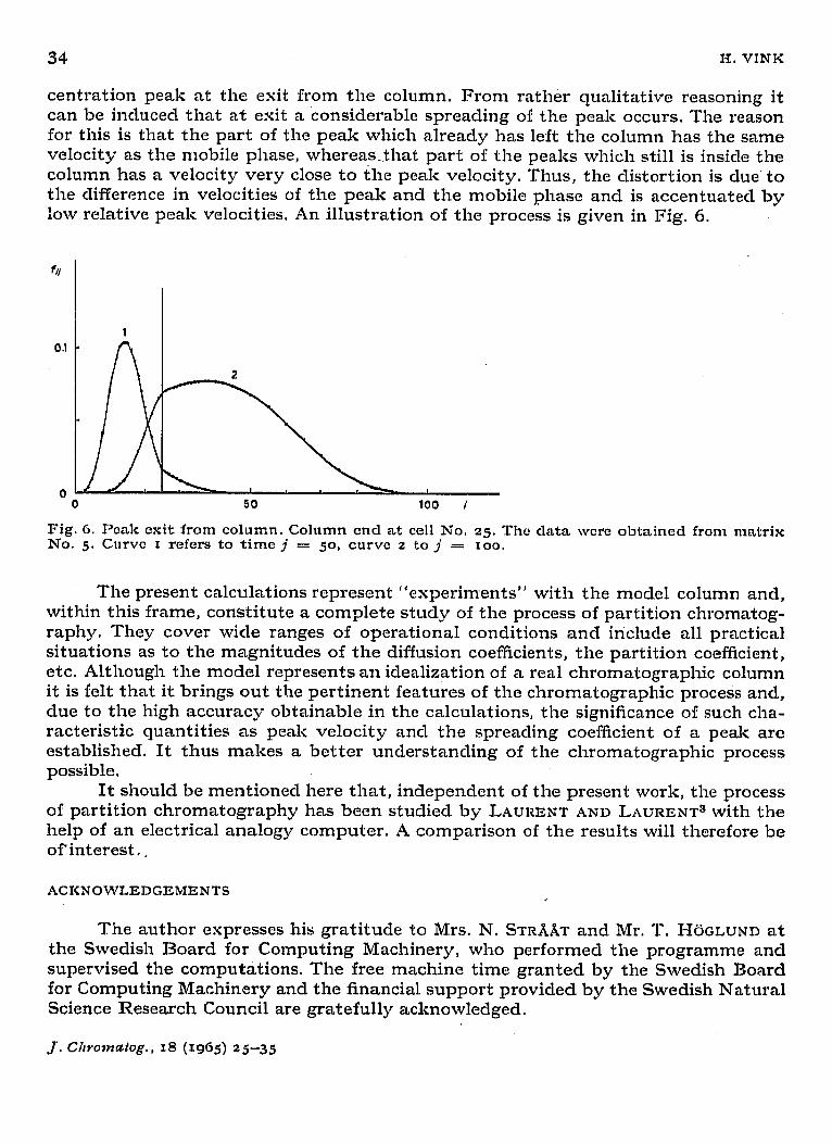
centration peak at the esit from the column. From rather qualitative reasoning it can be induced that at exit a considerable spreading of the peak occurs. The reason for this is that the part of the peak which already has left the column has the same velocity as the mobile phase, whereasthat part of the peaks which still is inside the column has a velocity very close to the peak velocity. Thus, the distortion is clue to the difference in velocities of the peak and the mobile phase and is accentuated by low relative peak velocities, An illustration of the process is given in Fig. 6.

f ii

0.1 1

li!! 50 100 I

Fig. 6. Pcalc exit from column. Column cncl at cell No. 25. The clsta were obtained from matrix No. 5. Curve I refers to time j = 50, curve 2 to j = IOO,

The present calculations represent “experiments” with the model column and, within this frame, constitute a complete study of the process of partition chromatog- raphy. They cover wide ranges of operational conditions and include all practical situations as to the magnitudes of the diffusion coefficients, the partition coefficient, etc. Although the model represents an idealization of a real chromatographic column it is felt that it brings out the pertinent features of the chromatographic process and, due to the high accuracy obtainable in the calculations, the significance of such cha- racteristic quantities as peak velocity and the spreading coefficient of a peak are established. It thus makes a better understanding of the chromatographic process possible.

It should be mentioned here that, independent of the present work, the process of partition chromatography has been studied by LAURENT AND LAURENT~ with the help of an electrical analogy computer, A comparison of the results will therefore be of interest.,

ACKNOWLEDGEMENTS

The author expresses his gratitude to Mrs. N. STRKAT and Mr. T. H~GLUND at the Swedish Board for Computing Machinery, who performed the programme and supervised the computations. The free machine time granted by the Swedish Board for Computing Machinery and the financial support provided by the Swedish Natural Science Research Council are gratefully acknowledged.

THEORY OF PARTITION CHROMATOGIlAPkZY. II. Y5

SUMMARY

The operation df a chromatographic column has been simulated by numerical calculations on a digital computer. The calculations cover wide ranges of operational conditions for a column and give a detailed characterizstion of the chromatographic process.

REFERENCES

s H. VINIC, J. CAronZafOg., 15 (IQ&+) 42%. z H. VINIC, Nnlwvc. 205 (1965) 73. 3 T. C. LAURENT AND E, P. LAURENT, J. Clwomatog., 16 (I&.+) 89.

J. Chtmtatog., IS (1965) 25-35