Embed Size (px)
Citation preview
Theory of DemandECON 212 Lecture 7
Tianyi Wang
Queen’s Univerisity
Winter 2013
Tianyi Wang (Queen’s Univerisity) Lecture 7 Winter 2013 1 / 46

Intro
Note: Quiz 1 can be picked up at Distribution Center.Second Quiz covers: Preferences, Budget and Optimal Choices.
Core of theory of demand: how does demand change in differentenviroments.
Can have many directions. We will look at:I effect of changes in price, andI effect of changes in income.
Tianyi Wang (Queen’s Univerisity) Lecture 7 Winter 2013 2 / 46

Effect of Changes in Price
What happens to optimal choices when price changes.
Derive demand function from consumer’s optimal choices.
Tianyi Wang (Queen’s Univerisity) Lecture 7 Winter 2013 3 / 46

Tianyi Wang (Queen’s Univerisity) Lecture 7 Winter 2013 4 / 46

Tianyi Wang (Queen’s Univerisity) Lecture 7 Winter 2013 5 / 46

Tianyi Wang (Queen’s Univerisity) Lecture 7 Winter 2013 6 / 46

Tianyi Wang (Queen’s Univerisity) Lecture 7 Winter 2013 7 / 46

Tianyi Wang (Queen’s Univerisity) Lecture 7 Winter 2013 8 / 46

Tianyi Wang (Queen’s Univerisity) Lecture 7 Winter 2013 9 / 46

Tianyi Wang (Queen’s Univerisity) Lecture 7 Winter 2013 10 / 46

Demand Function
Note, demand curve derived from definition: letting Px changes whileholding others constant.
See class notes for examples.
Tianyi Wang (Queen’s Univerisity) Lecture 7 Winter 2013 11 / 46

Demand Function (Cont’d)
Demand curve is also a "willingness to pay curve"I MRS says willness to substitute.I MRS = Px
Py , or willing to sacrificePxPy unites of y.
I To translate into value, PxPy ∗ Py = Px .I Willing to pay Px for additional unit of x .
Tianyi Wang (Queen’s Univerisity) Lecture 7 Winter 2013 12 / 46

Effect of Changes in Income
Income Consumption Curve (ICC): traces out optimal bundles on X-Yspace as income changes.
Engel curve (EC): depicts optimal choices on I-X space.
Normal good V .S . Inferior good.
I Normal: positive slope for both ICC and ECI Inferior: negative slope for both ICC and EC
With Quasilinear utility function, both are vertical line. (Math andintuition?)
Tianyi Wang (Queen’s Univerisity) Lecture 7 Winter 2013 13 / 46

Effect of Changes in Income
Income Consumption Curve (ICC): traces out optimal bundles on X-Yspace as income changes.
Engel curve (EC): depicts optimal choices on I-X space.
Normal good V .S . Inferior good.I Normal: positive slope for both ICC and EC
I Inferior: negative slope for both ICC and EC
With Quasilinear utility function, both are vertical line. (Math andintuition?)
Tianyi Wang (Queen’s Univerisity) Lecture 7 Winter 2013 13 / 46

Effect of Changes in Income
Income Consumption Curve (ICC): traces out optimal bundles on X-Yspace as income changes.
Engel curve (EC): depicts optimal choices on I-X space.
Normal good V .S . Inferior good.I Normal: positive slope for both ICC and ECI Inferior: negative slope for both ICC and EC
With Quasilinear utility function, both are vertical line. (Math andintuition?)
Tianyi Wang (Queen’s Univerisity) Lecture 7 Winter 2013 13 / 46

Market Demand
Horizontal summation of individual demand.
See class notes for examples.
Usually assume identical individuals.
Tianyi Wang (Queen’s Univerisity) Lecture 7 Winter 2013 14 / 46

Income and Substitution Effect
Does price increase always decreases demand (Giffen good)?
Decrease (increase) in price can have ambiguous effect.— relatively cheaper, buy more.— richer, buy less (inferior good).
These ambiguities include:— the effect of wage rates on labor supply.— the effect of interest rates on savings.
Price changes involve two seperate effects:—Substitution effect: good 1 becomes cheaper, more attractive thangood 2 (opp. cost changes)— Income effect: b/c good 1 is cheaper, can buy more of it with agiven amount of income. Purchasing power increased.
Tianyi Wang (Queen’s Univerisity) Lecture 7 Winter 2013 15 / 46

Substitution Effect
How to seperate?
1 keep relative price changes, take away (grant) money to keep sth. fixed.2 reimburse and hold the relative prices.
Hicks Decomposition: fix (initial) utility level.
Slutsky Decomposition: fix purchasing power (not income).
We will use Hicks below (clean intuition).—how much consumer would require in payment to accept a change.
Tianyi Wang (Queen’s Univerisity) Lecture 7 Winter 2013 16 / 46
Substitution Effect
How to seperate?1 keep relative price changes, take away (grant) money to keep sth. fixed.
2 reimburse and hold the relative prices.
Hicks Decomposition: fix (initial) utility level.
Slutsky Decomposition: fix purchasing power (not income).
We will use Hicks below (clean intuition).—how much consumer would require in payment to accept a change.
Tianyi Wang (Queen’s Univerisity) Lecture 7 Winter 2013 16 / 46

Substitution Effect
How to seperate?1 keep relative price changes, take away (grant) money to keep sth. fixed.2 reimburse and hold the relative prices.
Hicks Decomposition: fix (initial) utility level.
Slutsky Decomposition: fix purchasing power (not income).
We will use Hicks below (clean intuition).—how much consumer would require in payment to accept a change.
Tianyi Wang (Queen’s Univerisity) Lecture 7 Winter 2013 16 / 46

Tianyi Wang (Queen’s Univerisity) Lecture 7 Winter 2013 17 / 46

Tianyi Wang (Queen’s Univerisity) Lecture 7 Winter 2013 18 / 46

Tianyi Wang (Queen’s Univerisity) Lecture 7 Winter 2013 19 / 46

Tianyi Wang (Queen’s Univerisity) Lecture 7 Winter 2013 20 / 46

Tianyi Wang (Queen’s Univerisity) Lecture 7 Winter 2013 21 / 46

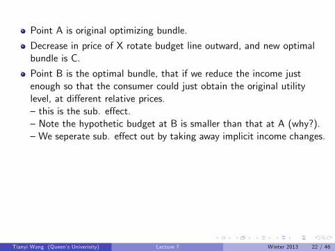
Point A is original optimizing bundle.
Decrease in price of X rotate budget line outward, and new optimalbundle is C.
Point B is the optimal bundle, that if we reduce the income justenough so that the consumer could just obtain the original utilitylevel, at different relative prices.— this is the sub. effect.—Note the hypothetic budget at B is smaller than that at A (why?).—We seperate sub. effect out by taking away implicit income changes.
Point C is the optimal bundle, that if we hold the new relative pricesand add back the income that we took away.— this is the inc. effect.—shift the hypothetic BC back to get implied changes in consumption.
See class note for examples.
Tianyi Wang (Queen’s Univerisity) Lecture 7 Winter 2013 22 / 46

Hicks substitution effect also know as Compensated Demand Curve.—consumers are compensated just enough to obtain the original utiliy.
Note sign of substitution effect must be negative
Sign of income effect can be positive or negative (normal v.s. inferior)
Therefore Giffen good must be inferior good.
Tianyi Wang (Queen’s Univerisity) Lecture 7 Winter 2013 23 / 46

Tianyi Wang (Queen’s Univerisity) Lecture 7 Winter 2013 24 / 46

Slustsky defines substitution effect by keeping purchasing powerconstant.
I both original BC and hypothetical BC go through A.I Note incomes are different.
Tianyi Wang (Queen’s Univerisity) Lecture 7 Winter 2013 25 / 46

Application: Consumption and Leisure Choice
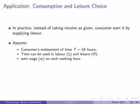
In practice, instead of taking income as given, consumer earn it bysupplying labour.
Assume:
I Consumer’s endowment of time T = 24 hours,I Time can be used in labour (L) and leisure (R).I earn wage (w) on each working hour.I Consumer values consumption (C ) and leisure (R), max U(C ,R).I Need to use wages to buy consumption good, Price = 1.
Formulate consumer’s problem, see class notes for example.
Tianyi Wang (Queen’s Univerisity) Lecture 7 Winter 2013 26 / 46

Application: Consumption and Leisure Choice
In practice, instead of taking income as given, consumer earn it bysupplying labour.
Assume:I Consumer’s endowment of time T = 24 hours,
I Time can be used in labour (L) and leisure (R).I earn wage (w) on each working hour.I Consumer values consumption (C ) and leisure (R), max U(C ,R).I Need to use wages to buy consumption good, Price = 1.
Formulate consumer’s problem, see class notes for example.
Tianyi Wang (Queen’s Univerisity) Lecture 7 Winter 2013 26 / 46
Application: Consumption and Leisure Choice
In practice, instead of taking income as given, consumer earn it bysupplying labour.
Assume:I Consumer’s endowment of time T = 24 hours,I Time can be used in labour (L) and leisure (R).
I earn wage (w) on each working hour.I Consumer values consumption (C ) and leisure (R), max U(C ,R).I Need to use wages to buy consumption good, Price = 1.
Formulate consumer’s problem, see class notes for example.
Tianyi Wang (Queen’s Univerisity) Lecture 7 Winter 2013 26 / 46
Application: Consumption and Leisure Choice
In practice, instead of taking income as given, consumer earn it bysupplying labour.
Assume:I Consumer’s endowment of time T = 24 hours,I Time can be used in labour (L) and leisure (R).I earn wage (w) on each working hour.
I Consumer values consumption (C ) and leisure (R), max U(C ,R).I Need to use wages to buy consumption good, Price = 1.
Formulate consumer’s problem, see class notes for example.
Tianyi Wang (Queen’s Univerisity) Lecture 7 Winter 2013 26 / 46
Application: Consumption and Leisure Choice
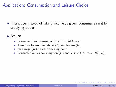
In practice, instead of taking income as given, consumer earn it bysupplying labour.
Assume:I Consumer’s endowment of time T = 24 hours,I Time can be used in labour (L) and leisure (R).I earn wage (w) on each working hour.I Consumer values consumption (C ) and leisure (R), max U(C ,R).
I Need to use wages to buy consumption good, Price = 1.
Formulate consumer’s problem, see class notes for example.
Tianyi Wang (Queen’s Univerisity) Lecture 7 Winter 2013 26 / 46

Application: Consumption and Leisure Choice
In practice, instead of taking income as given, consumer earn it bysupplying labour.
Assume:I Consumer’s endowment of time T = 24 hours,I Time can be used in labour (L) and leisure (R).I earn wage (w) on each working hour.I Consumer values consumption (C ) and leisure (R), max U(C ,R).I Need to use wages to buy consumption good, Price = 1.
Formulate consumer’s problem, see class notes for example.
Tianyi Wang (Queen’s Univerisity) Lecture 7 Winter 2013 26 / 46
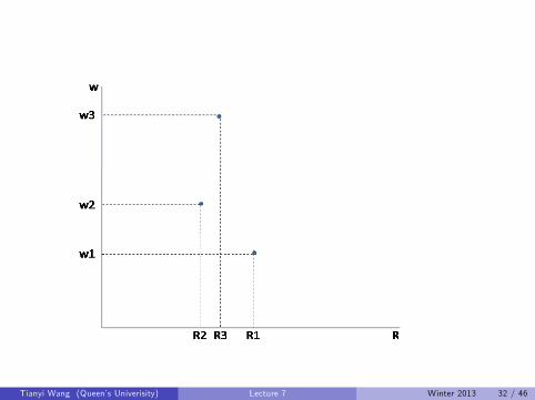
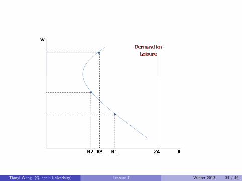
Backward bending labour supply
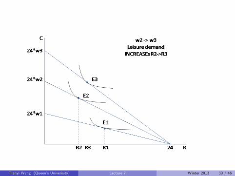
We can find demand for leisure from optimal choices, by varying wagerate (see graph below).
Since: supply of labour + demand for leisure = 24 hours.
L = T − R. (See graph below).
Tianyi Wang (Queen’s Univerisity) Lecture 7 Winter 2013 27 / 46

Tianyi Wang (Queen’s Univerisity) Lecture 7 Winter 2013 28 / 46

Tianyi Wang (Queen’s Univerisity) Lecture 7 Winter 2013 29 / 46
Tianyi Wang (Queen’s Univerisity) Lecture 7 Winter 2013 30 / 46

Tianyi Wang (Queen’s Univerisity) Lecture 7 Winter 2013 31 / 46
Tianyi Wang (Queen’s Univerisity) Lecture 7 Winter 2013 32 / 46

Tianyi Wang (Queen’s Univerisity) Lecture 7 Winter 2013 33 / 46
Tianyi Wang (Queen’s Univerisity) Lecture 7 Winter 2013 34 / 46

Tianyi Wang (Queen’s Univerisity) Lecture 7 Winter 2013 35 / 46

Tianyi Wang (Queen’s Univerisity) Lecture 7 Winter 2013 36 / 46

Substitution effect makes an hour of leisure more expensive.
Income effect increases your overall endowment.
Sub. effect if negative.
If leisure is normal good, consume more when income raises.– Income effect is positive.– Inc. effect counteracts sub. effect.
Labour supply curve bends baceward.
Tianyi Wang (Queen’s Univerisity) Lecture 7 Winter 2013 37 / 46

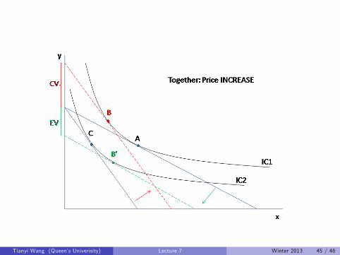
Compensating Variation and Equivalent Variation
Two ways to measure consumer welfare.I Price changes result in welfare change.I Rather than describe welfare in utility terms, we would like to describeit in terms of dollars.
Suppose price of X increases, (utility level drops):
1 Ask how much money to compensate a consumer, at the new price,such that she obtains her initial utility level.– This is Compensating Variation.
2 Ask how much money to take away from a consumer, at the initialprice, such that the effect is equivalent to the price change.– This is Equivalent Variation.
Tianyi Wang (Queen’s Univerisity) Lecture 7 Winter 2013 38 / 46

Tianyi Wang (Queen’s Univerisity) Lecture 7 Winter 2013 39 / 46

Tianyi Wang (Queen’s Univerisity) Lecture 7 Winter 2013 40 / 46

Tianyi Wang (Queen’s Univerisity) Lecture 7 Winter 2013 41 / 46

Tianyi Wang (Queen’s Univerisity) Lecture 7 Winter 2013 42 / 46

Tianyi Wang (Queen’s Univerisity) Lecture 7 Winter 2013 43 / 46

Tianyi Wang (Queen’s Univerisity) Lecture 7 Winter 2013 44 / 46
Tianyi Wang (Queen’s Univerisity) Lecture 7 Winter 2013 45 / 46

Note: these are pure income effects.
Note: Change in consumer surplus includes both inc. effect and sub.effect.
Which measure is higher depends on income elasticity.
However as the budget share of most goods are small, they arevirtually identical.
Tianyi Wang (Queen’s Univerisity) Lecture 7 Winter 2013 46 / 46