Theory and Applications of TAR Model with Two Threshold ...jb3064/papers/2012_The_theory... · THEORY AND APPLICATIONS OF TAR MODEL WITH TWO ... 1Threshold model with two threshold

Econometric Reviews, 31(2):142–170, 2012Copyright © Taylor & Francis Group, LLCISSN: 0747-4938 print/1532-4168 onlineDOI: 10.1080/07474938.2011.607100

THEORY AND APPLICATIONS OF TAR MODELWITH TWO THRESHOLD VARIABLES

Haiqiang Chen1, Terence Tai-Leung Chong2, and Jushan Bai3

1Wang Yanan Institute for Studies in Economics, Xiamen University, Fujian, China2Department of Economics and Institute of Global Economics and Finance,The Chinese University of Hong Kong, Hong Kong, China3Department of Economics, Columbia University, New York, New York, USA

� A growing body of threshold models has been developed over the past two decades to capturethe nonlinear movement of financial time series. Most of these models, however, contain a singlethreshold variable only. In many empirical applications, models with two or more thresholdvariables are needed. This article develops a new threshold autoregressive model which containstwo threshold variables. A likelihood ratio test is proposed to determine the number of regimesin the model. The finite-sample performance of the estimators is evaluated and an empiricalapplication is provided.

Keywords Bootstrapping; Likelihood ratio test; Misspecification; Threshold autoregressive model.

JEL Classification C22.

1. INTRODUCTION

A growing body of threshold models has been developed over thepast two decades to capture the nonlinear movement of financial timeseries. Tong (1983) develops a threshold autoregressive (TAR) model anduses it to predict stock price movements. A number of new models havebeen proposed since the seminal work of Tong (1983), including thesmooth transition threshold autoregressive model (STAR) of Chan andTong (1986) and the functional-coefficient autoregressive (FAR) model ofChen and Tsay (1993). Tsay (1998) develops a multivariate TAR model forthe arbitrage activities in the security market. Dueker et al. (2007) developa contemporaneous TAR model for the bond market.

Address correspondence to Terence Tai-Leung Chong, Department of Economics and Instituteof Global Economics and Finance, The Chinese University of Hong Kong, Hong Kong, China;E-mail: [email protected]

Dow

nloa

ded

by [

Hai

qian

g C

hen]

at 0

3:22

07

Nov

embe

r 20

11

Theory and Applications of TAR Model 143

Most of the aforementioned models, however, contain a singlethreshold variable only. In many empirical applications, a model with twoor more threshold variables is more appropriate. For example, Leeper(1991) divides the policy parameter space into four disjoint regionsaccording to whether monetary and fiscal policies are active or passive.Given these policy combinations, macroeconomic variables such as realoutput, inflation, and unemployment have different dynamics. Tiao andTsay (1994) divide the U.S. quarterly real Gross National Product (GNP)growth rate into four regimes according to the level and sign of the pastgrowth rate. Durlauf and Johnson (1995) split that cross-country GDPgrowth rate into different regimes according to the level of per capita realGDP and literacy rate. In modelling currency crises, Sachs et al. (1996),Frankel and Rose (1996), Kaminsky (1998), and Edison (2000) argue thatthe occurrence of currency crises hints at the values of fiscal reserves,foreign reserves, and interest rate differential between home countries andthe United States. In these examples, TAR models with multiple thresholdvariables can be used to describe the dynamics of different regimes.1

As the distributional theory is rather involved, no asymptotic result hasbeen developed for TAR models with multiple threshold variables.2 Thisarticle contributes to the literature by developing estimation and inferenceprocedures for TAR models with two threshold variables. Our model isapplied to identify the regimes of the Hong Kong stock market. The caseof Hong Kong is of interest because of its rising role as a global financialcenter. In 2006, Hong Kong became the world’s second most popular placefor Initial Public Offering (IPO) after London. In 2007, the Hong Kongstock market ranked fifth in the world, while its warrant market ranks topworldwide in terms of turnover. Using the historical prices of the HangSeng index and the market turnover as threshold variables, our estimationshows that the stock market of Hong Kong can be classified into a high-return stable regime, a low-return volatile regime, and a neutral regime.This is different from the conventional bull–bear classification.

The remainder of the article is organized as follows: Section 2 presentsthe model and discusses the estimation procedure. Section 3 derivesthe limiting distribution of the threshold estimators. Section 4 proposesa likelihood ratio test to determine the number of regimes. MonteCarlo simulations are conducted, and the performance of the estimationprocedure is evaluated in Section 5. An empirical application is providedin Section 6. Section 7 concludes the article.

1Threshold model with two threshold variables can also be applied to the cross-section offinancial data. For example, in the Fama and French (1992) model, one may use firm size andbook-to-market ratio as threshold variables to explain abnormal returns of a stock. Avramov et al.(2006) also sort stocks into different categories according to historical returns and liquidity level.

2A related empirical study is the nested threshold autoregressive (NeTAR) models of Astatkieet al. (1997).

Dow

nloa

ded

by [

Hai

qian

g C

hen]

at 0

3:22

07

Nov

embe

r 20

11

144 H. Chen et al.

2. TAR MODEL WITH TWO THRESHOLD VARIABLES

Consider the following TAR model with two threshold variables whichclassifies the observations yt into four regimes:

yt =

�(1)0 + �(1)

1 yt−1 + �(1)2 yt−2, � � � ,+�(1)

p1 yt−p1 + ut , when z1t ≤ �01, z2t ≤ �02

�(2)0 + �(2)

1 yt−1 + �(2)2 yt−2, � � � ,+�(2)

p2 yt−p2 + ut , when z1t ≤ �01, z2t > �02

�(3)0 + �(3)

1 yt−1 + �(3)2 yt−2, � � � ,+�(3)

p3 yt−p3 + ut , when z1t > �01, z2t ≤ �02

�(4)0 + �(4)

1 yt−1 + �(4)2 yt−2, � � � ,+�(4)

p4 yt−p4 + ut , when z1t > �01, z2t > �02

,

(1)

where

ztdef= (z1t , z2t) are the threshold variables;

�0def= (

�01,�02

) ∈ �, where � = [�1, �1] × [�2, �2] is a strict subset of the supportof zt � �0 is the threshold parameter vector pending to be estimated;

pj (j = 1, 2, 3, 4) is the order in each regime;

�(j) def= (�(j)0 , �(j)

1 , �(j)2 , � � � , �(j)

pj )′ are the structural parameters and �(i) �= �(j)

for some i �= j .3

The model is a linear AR model within each regime.4 The thresholdvariables z1 and z2 can be exogenous variables or functions of the lags ofyt .5 Given �yt , zt�

Tt=1, our objective is to estimate the threshold parameters

�0 and the structural parameters �(j). Without loss of generality, we let p =max �p1, p2, p3, p4� , and �(j)

q = 0 when q > pj , j = 1, 2, 3, 4. The model canbe rewritten as

yt =4∑

j=1

�(j)t

(�0

)(�

(j)0 +

p∑i=1

�(j)i yt−i + ut), (2)

3Restrictions on the structural parameters can be imposed so that there are less than fourregimes. For example, if �(1) = �(2) = �(3), the model will have two regimes only.

4An empirical example of the Model (1) is Tiao and Tsay’s (1994) four-regime TAR modelfor quarterly U.S. real GNP growth rates yt :

yt =

−0�015 − 1�076yt−1 + �1t , yt−1 ≤ yt−2 ≤ 0

0�63yt−1 − 0�76yt−2 + �2t , yt−1 > yt−2, yt−2 ≤ 0

0�006 + 0�43yt−1 + �3t , yt−1 ≤ yt−2, yt−2 > 0

0�433yt−1 + �4t , yt−1 > yt−2 > 0

�

In their model, the process is divided into four regimes by z1t = yt−2 and z2t = yt−1 − yt−2, andthe threshold values are set to zero. In practice, we need to estimate the threshold values.

5The model is a Self-Exciting Threshold Autoregressive (SETAR) model if the thresholdvariable is yt−d .

Dow

nloa

ded

by [

Hai

qian

g C

hen]

at 0

3:22

07

Nov

embe

r 20

11


where �(j)t

(�0

)is an indicator function which equals one when the

threshold condition is satisfied, and equals zero otherwise. Specifically,

�(1)t

(�0

) = I(z1t ≤ �01, z2t ≤ �02

),

�(2)t

(�0

) = I(z1t ≤ �01, z2t > �02

),

�(3)t

(�0

) = I(z1t > �01, z2t ≤ �02

),

�(4)t

(�0

) = I(z1t > �01, z2t > �02

)�

For analytical reasoning, it is convenient to rewrite the model (2) inthe following matrix form:

Y =4∑

j=1

Ij(�0)X�(j) + U , (3)

where

X = (x ′T , x

′T−1, � � � , x

′p+1)

′ =

1, yT−1, yT−2, � � � , yT−p

1, yT−2, yT−3, � � � , yT−p−1

� � � �1, yp , yp−1, � � � , y1

(T−p)×(p+1)

,

xt = (1, yt−1, � � � , yt−p)′ for t = p + 1, � � � ,T �

Ij(�0) = diag{�

(j)T

(�0

),�(j)

T−1

(�0

), � � � ,�(j)

p+1

(�0

)},

Y = (yT , yT−1, � � � , yp+1)′,

U = (uT ,uT−1, � � � ,up+1)′�

We make the following assumptions:

(A1) yt is stationary ergodic and E(y4t ) < ∞�(A2) �ut� is a sequence of independent and identical distributed (IID)

normal errors with zero mean and finite variance 2.(A3) The threshold variables z1t and z2t are strictly stationary and have

a continuous joint distribution F (�), which is differentiable withrespect to both variables. Let f (�) denote the corresponding jointdensity function and fi(�) = F (�)

�i. We assume that 0 < f (�) ≤ f <

∞; 0 < fi(�) ≤ fi < ∞ for i = 1, 2�

(A1) assumes that yt is stationary ergodic, which allows us to applythe law of large number. A sufficient condition for (A1) to hold is

Dow

nloa

ded

by [

Hai

qian

g C

hen]

at 0

3:22

07

Nov

embe

r 20

11

146 H. Chen et al.

maxj∑

i(|�(j)i |) < 1.6 (A2) assumes that �ut� is a sequence of i.i.d. normal

errors with finite second moment.7 (A3) requires the stationarity ofthe threshold variables. We also assume that the threshold variables arecontinuous with positive density everywhere, so that it is dense near �0 asthe sample size increases. This assumption is needed for the consistentestimation of threshold values.

Given � = (�1,�2), the conditional least square (CLS) estimator for �(j)

is defined as

�(j) (�) = (X′Ij(�)X )−1X

′Ij(�)Y ,

(j = 1, 2, 3, 4

), (4)

where

Ij(�) = diag{�

(j)T (�) ,�(j)

T−1 (�) , � � � ,�(j)p+1 (�)

}�

The residual sum of squares is

RSST (�) =∥∥∥∥

4∑j=1

Ij(�0)X�(j) + U −4∑

j=1

Ij(�)X �(j) (�)

∥∥∥∥2

,

and we define the estimator of �0 as the value that minimizes RSST (�):

� = argmin�∈�

RSST (�) � (5)

The structural estimators evaluated at the estimated threshold valuesare defined as

�(j)(�) = (X ′Ij(�)X )−1X ′Ij(�)Y � (6)

Appendix 2 shows the consistency of the estimators (�, �(j)(�)).

3. LIMITING DISTRIBUTION OF(�1, �2

)

In this section, the asymptotic joint distribution of the least-squaresestimator � is derived under the assumption that the magnitude of changegoes to zero at an appropriate rate. As pointed out by Hansen (2000), theassumption of decaying threshold effect is needed in order to obtain an

6See Chan (1993) and Hansen (1997).7In this article, we generalize the TAR model to the one with two threshold variables. The

error term ut is assumed to be i.i.d. normal in order to derive the asymptotic distribution ofthe threshold estimators. We can relax this assumption and allow for heteroskedasticity of ut . Theestimators will still be consistent. See Hansen (1997) for more discussion on the heteroskedasticerrors.

Dow

nloa

ded

by [

Hai

qian

g C

hen]

at 0

3:22

07

Nov

embe

r 20

11


asymptotic distribution of � free of nuisance parameters.8 For notationalsimplicity, we rewrite Model (2) as

Y = X�(1) +4∑

j=2

X (j)�0�(j) + U , (7)

where

X (j)�0

= Ij(�0

)X ,

(j = 2, 3, 4

)and

�(j) = �(j) − �(1),(j = 2, 3, 4

)�

For any given �, we define

X (j)� = Ij (�)X ,

(j = 1, 2, 3, 4

)�

Observe that X (i)′� X (j)

� = 0 if i �= j , and X′X (j)

� = X (j)′� X (j)

� �

Let X (j)0 = X (j)

�0, we have

X =4∑

j=1

X (j)0 =

4∑j=1

X (j)� �

We define the following conditional moment functionals:

D (�) = E(xtx ′

t | zt = �), (8)

V (�) = E(xtx ′

t u2t | zt = �

)� (9)

Let D = D(�0), V = V (�0). Under the assumption (A2), V = 2D� Wedefine block diagonal matrices D∗ = diag �D,D� and V ∗ = diag �V ,V �.9 Wealso need the following assumptions before the limiting distribution of �can be obtained. These assumptions mainly follow Hansen (1997, 2000).

(A4) M > Mj(�) > 0 for all � ∈ �, where M = E(xtx ′

t

),Mj (�) =

E(xtx ′

t�(j)t (�)

), j = 1, 2, 3, 4�

(A5) �T = (�(2)′, �(3)

′, �(4)

′)

′ = cT −� = (c ′2, c

′3, c

′4)

′T −�, 0 < � < 12 , c is a 3p-

dimensional constant vector and ci is a p-dimensional constant vectorfor i = 2, 3, 4.

8This approach is first used in the literature of change points (Bai, 1997) and applied to thethreshold model by Hansen (2000).

9Note that D and V are p × p matrices and D∗ and V ∗ are 2p × 2p matrices.

Dow

nloa

ded

by [

Hai

qian

g C

hen]

at 0

3:22

07

Nov

embe

r 20

11

148 H. Chen et al.

(A6) D(�) and V (�) are continuous at � = �0�(A7) d ′

1D∗d1 > 0, d ′

2D∗d2 > 0, where d1 = (c ′

2 − c ′4, c

′3)

′, d2 = (c ′2, c

′3 − c ′

4)′�

(A4) is the conventional full-rank condition which excludes perfectcollinearity. � is restricted to be a proper subset of the support of z�

(A5

)assumes that the parameter change is small and converges to zero at aslow rate when the sample size is large. Under this assumption, we are ableto make the limiting distribution of � free of nuisance parameters (Chan,1993). By letting �T go to zero, we reduce the rate of convergence of �from Op(T −1) to Op(T −1+2�) and obtain a simpler limiting distribution of�. (A6) requires the moment functionals to be continuous so that one canobtain the Taylor expansion around �0� This condition excludes regime-dependent heteroskedasticity. (A7) excludes the continuous thresholdmodel.10 Moreover, d ′

1D∗d1 > 0 and d ′

2D∗d2 > 0 impose the identification

condition for �01 and �02, respectively.11

Theorem 1. Under assumptions (A1) to (A7), we have

T 1−2� T((�1 − �01), (�2 − �02)

) = (r1, r2)

d→ argmax−∞<r1<∞,−∞<r2<∞

[−12

∣∣r1∣∣ + W1 (r1) − 12

∣∣r2∣∣ + W2(r2)],

where

T =((d ′

1D∗d1)f 0

1

2,(d ′

2D∗d2)f 0

2

2

),

and Wi(ri) is a two-sided Brownian motion on the real line defined as

Wi(ri) =

�i1(−ri) if ri < 00 if ri = 0�i2(ri) if ri > 0

,

�i(ri), i = 1, 2, and j = 1, 2 are four independent standard Brownian motions on[0,∞)�

Proof. See Appendix 3. �

10This article focuses on the discontinuous threshold effect. For continuous threshold models,one is referred to Chan and Tsay (1998).

11Note that d1 = (c ′2 − c ′

4, c′3)

′ measures the size of the threshold effect for the first thresholdvariable z1, while d2 = (c ′

2, c′3 − c ′

4)′ measures the size of the threshold effect for the second threshold

variable z2. When c2 = c4 �= 0 and c3 = 0, we obtain a single threshold model with only two regimesseparated by z2 = �02. In this case, �01 is not identified. When c2 = 0 and c3 = c4 �= 0, we have asingle threshold model with only two regimes separated by z1 = �01 and �02 is not identified.

Dow

nloa

ded

by [

Hai

qian

g C

hen]

at 0

3:22

07

Nov

embe

r 20

11


The result of Hansen (1997) is a special case of Theorem 1 with d1 = 0or d2 = 0. One can also use Theorem 1 to simulate the confidence intervalof (�1, �2)� The parameter ratio T can be estimated by a polynomialregression or kernel regression. See Hansen (1997, 2000).

4. TESTING FOR AND ESTIMATION OF THE THRESHOLD

To determine the number of regimes, we first consider the nullhypothesis of no threshold effect:

H0 : �(1) = �(2) = �(3) = �(4)�

Under the null hypothesis, there is only one regime. We define alikelihood ratio test statistic as

JT = max�∈�

(T − p)2 − 2(�)

2(�)� (10)

(T − p )2 is the residual sum of squares under the null hypothesis,while (T − p)2(�) is the residual sum of squares under the alternatives. IfH0 cannot be rejected, then the model is a simple AR model. Rejection ofthe null hypothesis suggests the existence of more than one regimes. Thethreshold estimator is defined as � = argmin 2(�) = argmax JT (�). Since� is not identified under the null hypothesis, the asymptotic distributionof JT (�) is not a standard �2� Hansen (1996) shows that the asymptoticdistribution can be approximated by the following bootstrap procedure.

Let u∗t (t = 1, � � � ,T ) be i.i.d. N (0, 1), and set y∗

t = u∗t . Next, we regress

y∗t on xt = (1, y∗

t−1, y∗t−2, � � � , y

∗t−p) to obtain the J ∗

T (�) = (T − p) ∗2−∗2(�)∗2(�) and

J ∗T = max�∈� J ∗

T (�)�The distribution of J ∗

T converges weakly in probability to thedistribution of JT under the null hypothesis. Therefore, one can use thebootstrap value of J ∗

T to approximate the asymptotic null distribution of JT �The percentage of draws where the simulated statistic under H0 exceedsthe one obtained from the original sample is our bootstrapping p-value.The null hypothesis will be rejected if the p-value is small.

Rejection of the null hypothesis implies the presence of thresholdeffects. To determine the number of regimes, a general-to-specificapproach is adopted. First, a three-regime model is tested against a four-regime model. Each of the following hypotheses

(I) H0 : �(1) = �(2);(II) H0 : �(1) = �(3);(III) H0 : �(1) = �(4);(IV) H0 : �(2) = �(3);

Dow

nloa

ded

by [

Hai

qian

g C

hen]

at 0

3:22

07

Nov

embe

r 20

11

150 H. Chen et al.

(V) H0 : �(2) = �(4);(VI) H0 : �(3) = �(4)�

is tested against the alternative hypothesis

H1 : there are four regimes�

A likelihood ratio test

JT (�) = (T − p)20(�) − 2

1(�)

21(�)

(11)

is used to test these pairs of hypotheses, where (T − p)20(�) is the

residual sum of squares under H0, and (T − p)21(�) is the residual sum

of squares under H1. A parametric bootstrap method is applied to obtainthe critical value. � is the estimated value from the unrestricted model.Let y∗

t = ∑4j=1(�

(j)0 + ∑p

i=1 �(j)i y∗

t−i)�(j)t (�) + u∗

t , where u∗t are i.i.d. N (0, 1)

and �(j)′i s are estimated under the restricted model. We regress y∗

t on xt =(1, y∗

t−1, y∗t−2, � � � , y

∗t−p) to obtain J ∗

T (�) = (T − p) ∗20 (�)−∗2

1 (�)

∗21 (�)

, and repeat thisprocedure a large number of times to calculate the percentage of draws forwhich the simulated statistic exceeds the actual value. The null is rejectedif this p-value is too small.

Rejection of all the null hypotheses (I)–(VI) implies the existence offour regimes. If any one of them is accepted, then there are less than fourregimes, and we proceed to test a two-regime model against a three-regimemodel. For instance, if (I ) H0 : �(1) = �(2) is accepted, then there are atmost three regimes, and we proceed to test the two-regime model againstthe three-regime model. The following three hypotheses are tested usingJT (�):

H0 : �(1) = �(2) = �(3);

H0 : �(1) = �(2) = �(4);

H0 : �(1) = �(2), �(3) = �(4)�

The alternative hypothesis is:

H1 : There are three regimes with �(1) = �(2)�

If all the above null hypotheses are rejected, we conclude that there arethree regimes. Otherwise, we conclude that the model has two regimes. Inempirical studies, one can estimate the autoregressive order, the thresholdvalue, and the coefficients of the TAR model via the following procedure.

Dow

nloa

ded

by [

Hai

qian

g C

hen]

at 0

3:22

07

Nov

embe

r 20

11


Step 1: First, a first-order TAR model is estimated:

yt =4∑

j=1

(�(j)0 + �

(j)1 yt−1)�

(j)t (�) + ut ,

and the initial threshold estimate �T is obtained.The first-order model is estimated for simplicity purposes (Chong,

2001). The initial threshold estimate will still be consistent even if the truemodel is not of the first-order (Bai et al., 2008; Chong, 2003).12

Step 2: Given the threshold values obtained from step 1, we usethe Akaike Information Criterion (AIC) (Tsay, 1998) to select theautoregressive order in each regime. In our case,

AICj(pj) = nj ln[RSSj(�T )/nj ] + 2(pj + 1), (12)

where

nj is the number of observations in the j th regime;pj is the order of autoregression in the j th regime;RSSj(�T ) is the residual sum of squares for the j th regime.

Define

pj = argminpj∈�1,2,��,Pmax�

AICj(pj), (13)

where Pmax is the maximum order considered in the model. The AIC forthe whole model can be written as

NAIC =s∑

j=1

AICj(pj), (14)

where s is the number of regimes.

Step 3: Perform the sequential likelihood ratio test to determine thenumber of regimes.

Step 4: Use the result obtained from step 3 to refine the thresholdvalues, and repeat steps 2 and 3 until all the estimates converge.

12The proof is available upon request.

Dow

nloa

ded

by [

Hai

qian

g C

hen]

at 0

3:22

07

Nov

embe

r 20

11

152 H. Chen et al.

5. SIMULATIONS

In the previous section, it is argued the threshold value can beconsistently estimated even if we start with a misspecified model in step1. This result is obtained by Chong (2003) and Bai et al. (2008). Thefollowing experiments examine the consistency of the threshold estimatorunder model misspecifications.

The experiment is set up as follows:Sample size: T = 200;Number of replications: N = 500;ut ∼ N (0, 1), �t ∼ N (0, 1), z1t ∼ N (0, 1);Pmax = 10�We consider two cases for z2t : (i) z2t ∼ N (0, 1), and (ii) z2t = z1t + �t �

The following data generating processes are examined:

DGP 1: yt = (0�3yt−1 + 0�3yt−2)I (z1t ≤ 0 or z2t ≤ 0) + (−0�3yt−1 − 0�3yt−2)I(z1t > 0 and z2t > 0) + ut ;

DGP 2: yt = 0�3yt−1I (z1t ≤ 0 or z2t ≤ 0) − 0�3yt−1I (z1t > 0 and z2t > 0) + ut �

Three misspecified models are estimated:

Model A: yt = ∑4j=1 �

(j)1 yt−1�

(j)t (�) + ut ;

Model B: yt = ∑4j=1(�

(j)1 yt−1 + �

(j)2 yt−2)�

(j)t (�) + ut ;

Model C: yt = �(1)1 yt−11(z1t ≤ �1) + �(2)

1 yt−11(z1t > �1) + ut .

Model A underestimates the autoregressive order p, while Model Boverestimates the autoregressive order p� Both of them overestimate thenumber of regimes. The estimation results are reported in Table 1. For allmisspecified estimated models, �1 and �2 converge to the true thresholdvalue 0. The results for models A and B suggest that the consistency ofthe threshold estimators is unaffected by the misspecification of regressors.Therefore, if the number of threshold variables is known, one can obtaina preliminary and consistent threshold estimate using the simplest modelpossible. The preliminary estimate of the threshold value can be used toobtain the estimates of other parameters of interest. In the context ofour model, such a preliminary threshold value allows us to determinethe number of regimes, as well as the order and parameters of theautoregressive model within each regime.

The results of Chong (2003) and Bai et al. (2008) apply to cases wherethe threshold variables are correctly specified. Model C underspecifies thenumber of threshold variables. The results for Model C show that the

Dow

nloa

ded

by [

Hai

qian

g C

hen]

at 0

3:22

07

Nov

embe

r 20

11


TABLE 1 The simulation results

DGP Estimated model z2t �1 Var (�1) �2 Var (�2)

1 A N (0, 1) 0�007 0�030 −0�002 0�0251 A z1t + �t −0�002 0�036 −0�003 0�0292 B N (0, 1) −0�001 0�025 −0�005 0�0342 B z1t + �t −0�006 0�025 0�002 0�0272 C N (0, 1) −0�015 0�682 C z1t + �t −0�19 0�28

estimators of the single threshold-variable model may not be consistent inthe presence of two dependent threshold variables.

6. EMPIRICAL APPLICATION

Our model is applied to the daily return series of the Hang Seng Index.The Hong Kong stock market is studied because of its rising role as aglobal financial center. In 2006, Hong Kong becomes the world’s secondmost popular place for IPO after London. In 2007, the Hong Kong stockmarket ranks fifth in the world, and its warrant market ranks first globallyin terms of turnover. Most of the previous studies in the literature usethe first lagged return as the threshold variable to identify the marketregimes. Such a classification method does not take investors’ sentimentinto account and does not consider the information of market turnover.In this article, we use the past information of price and market turnover toconstruct our threshold variables. Our sample period runs from January 31995 to January 13, 2005. The return series is defined as the log-differenceof the Hang Seng Index (HSI). There are over 2500 observations in oursample. Figures 1 and 2 show the time series data for daily return andmarket turnover.

The two threshold variables are analogous to those of Granville (1963)and Lee and Swaminathan (2000). We define the first threshold variableas

Rapt = PMA20tPMA250t

, (15)

where

PMA250t =∑250

j=1 pt−j

250, PMA20t =

∑20j=1 pt−j

20�

PMA250t is the average price for the past 250 trading days.PMA20t is the average price for the past 20 trading days.

Dow

nloa

ded

by [

Hai

qian

g C

hen]

at 0

3:22

07

Nov

embe

r 20

11

154 H. Chen et al.

FIGURE 1 Hand Seng index return series.

The variable is a ratio of two moving averages, which is similar tothat of Hong and Lee (2003). In particular, the 250-day moving average,which is widely used by investors to define the market state, is employed.If the price rises above (falls below) the 250-day moving average, anaverage investor who has taken a long position in the previous year (about250 trading days) has made a profit (loss), suggesting that the marketsentiment should be good (bad). To reduce noise, we use the crossing

FIGURE 2 Hand Seng index daily trading volume.

Dow

nloa

ded

by [

Hai

qian

g C

hen]

at 0

3:22

07

Nov

embe

r 20

11


of the 20-day and 250-day moving averages to help identify the marketregimes.

The second threshold variable contains the information of the marketturnover, which has been widely used to measure the liquidity of themarket, see Amihud and Mendelson (1986), Brennan et al. (1998),and Amihud (2002) among others. Several studies have shown thatthe autocorrelation in stock returns is related to turnover or tradingvolume. For example, Campbell et al. (1993) find that the first-order dailyreturn autocorrelation tends to decline with turnover, and the returnsaccompanied by high volume tend to be reversed more strongly. Llorenteet al. (2002) point out that intensive trading volume can help to identifythe periods in which shocks occur. Therefore, we define the secondthreshold variable as

Ravt = log(turnovert−1) − MAVt−1, (16)

where

MAVt =∑250

j=1 log(turnovert−j)

250�

Figure 3 shows the two threshold variables Rapt and Ravt .

FIGURE 3 The two threshold variables.

Dow

nloa

ded

by [

Hai

qian

g C

hen]

at 0

3:22

07

Nov

embe

r 20

11

156 H. Chen et al.

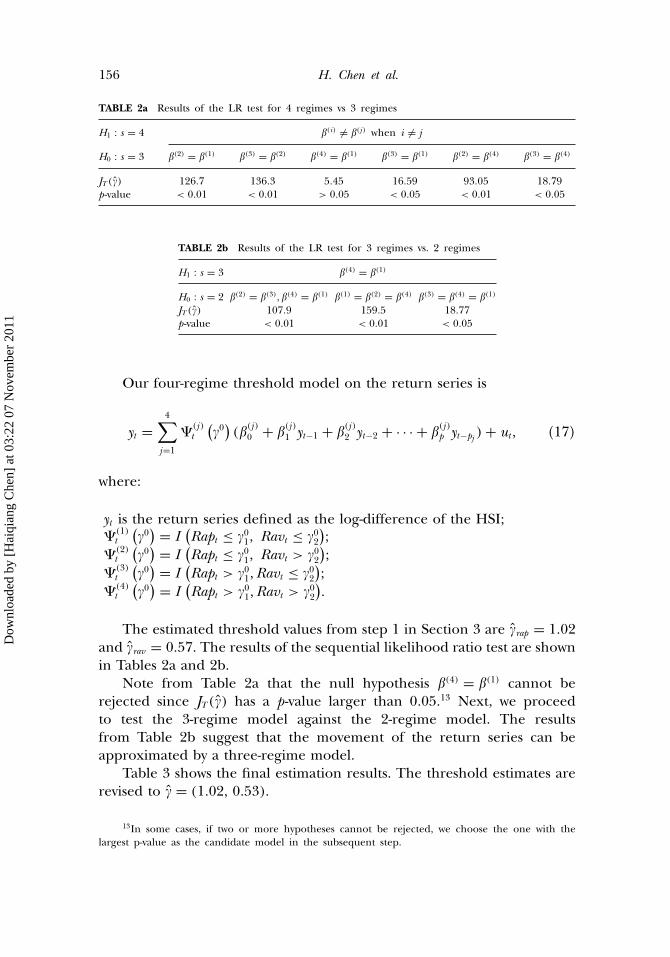
TABLE 2a Results of the LR test for 4 regimes vs 3 regimes

H1 : s = 4 �(i) �= �(j) when i �= j

H0 : s = 3 �(2) = �(1) �(3) = �(2) �(4) = �(1) �(3) = �(1) �(2) = �(4) �(3) = �(4)

JT (�) 126�7 136�3 5�45 16�59 93�05 18�79p-value < 0�01 < 0�01 > 0�05 < 0�05 < 0�01 < 0�05

TABLE 2b Results of the LR test for 3 regimes vs. 2 regimes

H1 : s = 3 �(4) = �(1)

H0 : s = 2 �(2) = �(3), �(4) = �(1) �(1) = �(2) = �(4) �(3) = �(4) = �(1)

JT (�) 107�9 159�5 18�77p-value < 0�01 < 0�01 < 0�05

Our four-regime threshold model on the return series is

yt =4∑

j=1

�(j)t

(�0

)(�

(j)0 + �

(j)1 yt−1 + �

(j)2 yt−2 + · · · + �

(j)p yt−pj ) + ut , (17)

where:

yt is the return series defined as the log-difference of the HSI;�(1)

t

(�0

) = I(Rapt ≤ �01, Ravt ≤ �02

);

�(2)t

(�0

) = I(Rapt ≤ �01, Ravt > �02

);

�(3)t

(�0

) = I(Rapt > �01,Ravt ≤ �02

);

�(4)t

(�0

) = I(Rapt > �01,Ravt > �02

).

The estimated threshold values from step 1 in Section 3 are �rap = 1�02and �rav = 0�57. The results of the sequential likelihood ratio test are shownin Tables 2a and 2b.

Note from Table 2a that the null hypothesis �(4) = �(1) cannot berejected since JT (�) has a p-value larger than 0�05�13 Next, we proceedto test the 3-regime model against the 2-regime model. The resultsfrom Table 2b suggest that the movement of the return series can beapproximated by a three-regime model.

Table 3 shows the final estimation results. The threshold estimates arerevised to � = (1�02, 0�53)�

13In some cases, if two or more hypotheses cannot be rejected, we choose the one with thelargest p-value as the candidate model in the subsequent step.

Dow

nloa

ded

by [

Hai

qian

g C

hen]

at 0

3:22

07

Nov

embe

r 20

11


TABLE 3 The estimated TAR model

Regime Estimation results

I yt = 0�0003 + 0�065yt−1, if Rapt > 1�02 and Ravt ≤ 0�53II yt = 0�0067 − 0�3yt−1 − 0�4yt−2 + 0�18yt−3 + 0�09yt−4 − 0�12yt−5 + 0�54yt−6

−0�5yt−7 − 0�18yt−8, if Rapt ≤ 1�02 and Ravt > 0�53III yt = 0�00014 + 0�096yt−1 otherwise

Figure 4 plots the estimated residuals of the model.14

Using the Markov-switching model, Maheu and McCurdy (2000) dividethe stock market into a high-return stable regime and a low-return volatileregime. From Table 3, we are able to classify the stock market of HongKong into three regimes. Since high turnover is usually associated withvolatile returns Karpoff (1987); Foster and Viswanathan (1995), RegimeI generated by our model corresponds to the high-return stable regime,while Regime II is the low-return volatile regime.15 Regime III is a neutralregime. Table 4 shows a chronology of major events affecting the HongKong stock market between 1996 and 2005.16

7. CONCLUSION

Conventional threshold models only allow for a single thresholdvariable. In many applications, the use of multiple threshold variables isneeded. In this article, a new TAR model with two threshold variables isdeveloped. In addition, the consistency and limiting distribution of theestimators are established. A likelihood ratio test is also constructed todetect the threshold effect. Our model is applied to identify the regimesof the Hong Kong stock market. The two threshold variables used in

14A Ljung–Box test has been conducted and the results suggest that the residuals are whitenoise. The details of the test can be obtained from the authors upon request.

15Note that the first-order coefficient for Regime I is 0.065, which is positive as compared tothat of −0�3 for Regime II. This agrees with Campbell et al. (1993) that the first-order daily returnautocorrelation tends to decline when turnover increases.

16We associate the estimated regimes with these major events. For example, the establishmentof the Hong Kong Special Administration Region in July 1997 falls into Regime I. During theAsian Financial Crisis, the crash of the stock market of Hong Kong and the burst of the propertymarket fall into Regime II. The market experiences a volatile year in the millennium. Driven bythe technology bubble and the accession of China to the World Trade Organization, the HangSeng Index reaches a record high of 18301 in March 2000. However, the burst of the bubble in2000 brings the stock market back into Regime II again. The market enters Regime I at the endof 2001. Note that the Hong Kong stock market is not seriously affected by the 911 incident. Theaccession of China to the World Trade Organization in 2001 is a good news for Hong Kong. Inthe beginning of 2003, the outbreak of the Severe Acute Respiratory Syndrome (SARS) threatensthe economy. The market switches from Regime I to Regime II during the SARS period, but itrebounds sharply in the second half of the year. In June, China and Hong Kong sign the CloserEconomic Partnership Arrangement (CEPA), a free trade agreement between Hong Kong andChina which gives Hong Kong a preferential access to the Chinese market.

Dow

nloa

ded

by [

Hai

qian

g C

hen]

at 0

3:22

07

Nov

embe

r 20

11

158 H. Chen et al.

FIGURE 4 The residual series.

this article are analogous to those of Granville (1963) and Lee andSwaminathan (2000). Unlike the conventional bull–bear classification, itis shown that the Hong Kong stock market can be classified into threeregimes, namely, a high-return stable regime, a low-return volatile regime,and a neutral regime. It should be mentioned that our model assumes asingle threshold for each threshold variable. It can be extended to allowfor the existence of multiple thresholds (Gonzalo and Pitarakis, 2002). Forexample, if there are two threshold variables and each threshold variablehas two threshold values, then the model can have at most nine regimes.One may also define the threshold condition as a nonlinear function ofthe two threshold variables. Finally, one may relax the i.i.d. assumptionof the error term to allow for serial dependence and regime-dependentheteroskedasticity. Such extensions, however, are beyond the scope of thisarticle and are left for future research.

TABLE 4 A Chronology of the Hong Kong stock market and the corresponding regimes

Date Event Regime

1997.7 The establishment of the Hong Kong Special Administration Region I1997.10.23 Asian currency turmoil triggered by the floating of Thai Baht II1998.1–1999.3 The burst of the property market III, II1999.9–2000.3 Global technology stock boom and the admission of China into I, III

the World Trade Organization (WTO)2000.4–2000.6 The burst of the high-tech bubble II, III2001.9.11 The 911 incident I2001.11.13 The accession of China to the WTO I2003.2–2003.6 The outbreak of SARS I, II2003.6.29 The launch of Closer Economic Partnership Arrangement with China I

Dow

nloa

ded

by [

Hai

qian

g C

hen]

at 0

3:22

07

Nov

embe

r 20

11


APPENDIX 1: LEMMAS

Throughout the appendix, let ‖A‖ = (tr (A′A))1/2 denote the Euclideannorm of a matrix A� Let ‖A‖r = (E |A|r )1/r denote the Lr -norm of a randommatrix and ⇒ denote weak convergence with respect to the uniformmetric.

Let

xt = (1, yt−1, yt−2, � � � , yt−p)′ for t = p + 1, p + 2, � � � ,T ,

X = (x ′T , x

′T−1, � � � , x

′p+1)(T−p)×(p+1),

Y = (yT , � � � , yp+1)′,

U = (uT ,uT−1, � � � ,up+1)′,

Ij(�) = diag{�

(j)T (�) ,�(j)

T−1 (�) , � � � ,�(j)p+1 (�)

},

where �(j)t (�) is defined in Section 2.

Let M and Mj(�) be moment functionals defined as

M = E(xtx ′

t

), Mj (�) = E

(xtx ′

t�(j)t (�)

), j = 1, 2, 3, 4�

Lemma 1. Under assumptions (A1)–(A2), it can be shown that:

(a) 1T X

′Xp→ M ;

(b) 1T X

′Up→ 0�

Proof. The proof is straightforward by applying the law of large numberfor stationary ergodic processes. �

Lemma 2. For any � ∈ �, under assumptions (A1)–(A3), we have for j =1, 2, 3, 4:

(a) 1T X

′Ij(�)Xp→ Mj(�);

(b) 1T X

′Ij(�)Up→ 0;

(c) 1T (X

′Ij(�)U )′(X ′Ij(�)U )p→ E(xtx ′

t u2t �

(j)t (�)) = 2Mj(�)�

Proof. The proof of part (a) for j = 1 is similar to the proof of LemmaA1 in Hansen (1996) by replacing �wt ≤ �� with �z1t ≤ �1, z2t ≤ �2�. For j =2, we have 1

T X′I2(�)X = 1

T

∑xtx ′

t �z1t ≤ �1� − 1T

∑xtx ′

t �z1t ≤ �1, z2t ≤ �2�p→

E(xtx ′

t �z1t ≤ �1�) − E

(xtx ′

t �z1t ≤ �1, z2t ≤ �2�) = M2 (�). A similar proof can

be applied to the cases where j = 3 and 4. The proofs for (b) and (c) areanalogous and are therefore skipped. �

Dow

nloa

ded

by [

Hai

qian

g C

hen]

at 0

3:22

07

Nov

embe

r 20

11

160 H. Chen et al.

APPENDIX 2: CONSISTENCY OF ESTIMATORS

To prove the consistency of the estimator � = argmin�∈� RSST (�), itsuffices to show that RSST (�) converges uniformly to a function b(�) whichis minimized at �0� For simplicity, denote �(j) = �(j)(�) for j = 1, 2, 3, 4. LetY (�) = ∑4

j=1 Ij(�)X �(j). The residual sum of squares can be written as

RSST (�) = ‖Y − Y (�)‖2 = Y ′Y − Y (�)′Y (�)

=4∑

j=1

(�(j)′X ′Ij(�0)X�(j) − �(j)′X ′Ij(�)X �(j)

)

+ 24∑

j=1

U ′Ij(�0)X�(j) + U ′U �

Next, we prove that RSST (�) has a unique minimum at � = �0. Wepartition the threshold space into four regions.

Case 1: �1 ≤ �01 and �2 ≤ �02Using Lemmas 1 and 2, and the facts that

I1(�)I1(�0) = I1(�), I1(�)Ij(�0) = 0 for j = 2, 3, 4,

I2(�)I1(�0) = I2(�) − I2(�1, �02), I2(�)I2(�0) = I2(�1, �02),

I2(�)Ij(�0) = 0, for j = 3, 4,

I3(�)I1(�0) = I3(�) − I3(�01, �2), I3(�)I2(�0) = 0,

I3(�)I3(�0) = I3(�01, �2), I3(�)I4(�0) = 0,

I4(�)I1(�0) = I1(�0) + I1(�) − I1(�01, �2) − I1(�1, �02),

I4(�)I2(�0) = 0, I4(�)I3(�0) = I4(�01, �2) − I4(�0), I4(�)I4(�0) = I4(�0),

it can be shown that

�(1) = (X ′I1(�)X )−1X ′I1(�)Y

= (X ′I1(�)X )−1X ′I1(�)[ 4∑

j=1

Ij(�0)X�(j) + U]

= �(1) + 1√T

(X ′I1(�)X

T

)−1(X ′I1(�)U√T

)p→ �(1),

�(2) = (X ′I2(�)X )−1X ′I2(�)Yp→ M−1

2 (�)(M2(�) − M2(�1, �02))(�(1) − �(2)) + �(2),

Dow

nloa

ded

by [

Hai

qian

g C

hen]

at 0

3:22

07

Nov

embe

r 20

11


�(3) = (X ′I3(�)X )−1X ′I3(�)Yp→ M−1

3 (�)(M3(�) − M 03 (�

01, �2))(�

(1) − �(2))

+ M−13 (�)M3(�

01, �2)(�

(3) − �(2)) + �(2),

�(4) = (X ′I4(�)X )−1X ′I4(�)Yp→ M−1

4 (�)[M4(�

0) − M4(�01, �2) − M4(�1, �02) + M4(�)

](�(1) − �(2))

+ M−14 (�)M4(�

0)(�(4) − �(2))

+ M−14 (�)(M4(�

01, �2) − M4(�

0))(�(3) − �(2)) + �(2)�

Therefore,

1T

(RSST (�) − U ′U

)= 1

T

4∑j=1

(�(j)′X ′Ij(�0)X�(j) − �(j)′X ′Ij(�)X �(j)

)+ 2

T

4∑j=1

U ′Ij(�0)X�(j)

=4∑

j=1

�(j)′Mj(�0)(�(j) − �(2))

−[�(1)′M1(�) + �(2)′(M2(�) − M2(�1, �02))

](�(1) − �(2))

+ �(3)′[M3(�) − M3(�01, �2)](�(1) − �(2))

+ �(4)′[M4(�0) − M4(�

01, �2) − M4(�1, �02) + M4(�)](�(1) − �(2))

−[�(3)′M3(�

01, �2) + �(4)′(M4(�

01, �2) − M4(�

0))](�(3) − �(2))

− �(4)′M4(�0)(�(4) − �(2)) + op(1)

= (�(1) − �(2))′[M1(�0) − M1(�) − M−1

2 (�)(M2(�) − M2(�1, �02))2

− M−13 (�)(M3(�) − M3(�

01, �2))

2

− M−14 (�)(M4(�

0) − M4(�01, �2) − M4(�1, �02) + M4(�))

2] × (�(1) − �(2))

+ (�(3) − �(2))′[M3(�0) − M−1

4 (�)(M4(�01, �2) − M4(�

0))2

− M−13 (�)(M3(�

01, �2))

2](�(3) − �(2))

+ (�(4) − �(2))′ [M4(�0) − M−1

4 (�)(M4(�0))2

](�(4) − �(2)) + op(1)

= (�(1) − �(2))′Q1(�(1) − �(2)) + (�(3) − �(2))′Q2(�

(3) − �(2))

+ (�(4) − �(2))′Q3(�(4) − �(2)) + op(1)

= b1(�) + op(1)�

Dow

nloa

ded

by [

Hai

qian

g C

hen]

at 0

3:22

07

Nov

embe

r 20

11

162 H. Chen et al.

For any �1 ≤ �01 and �2 ≤ �02, it is obvious that Q3 is positive semidefinitesince M4(�) > M4(�

0)� Meanwhile, using the following results:

M1(�0) − M1(�) = E

(xtx ′

t�(1)t (�)

)= E(xtx ′

t [�(2)t (�) − �(2)

t (�1, �02) + �(3)t (�)

− �(3)t (�01, �2) + �(4)

t (�0) − �(4)t (�01, �2)

− �(4)t (�1, �02) + �(4)

t (�)])= M2(�) − M2(�1, �02) + M3(�) − M3(�

01, �2)

+ M4(�0) − M4(�

01, �2) − M4(�1, �02) + M4(�),

M3(�0) = M4(�

01, �2) − M4(�

0) + M3(�01, �2),

it can be shown that Q1 and Q2 are positive semidefinite. Thus, b1(�) ≥b1(�0) = 0, and the equation holds if and only if � = �0�

By analogy, for the remaining three cases,

1T

(RSST (�) − U ′U

) = bj(�) + op(1) and

bj(�) ≥ bj(�0) = 0 for j = 2, 3, 4�

Define a non-stochastic function b(�) as bj(�) for the j th case, we have

sup�∈�

∣∣∣∣ 1T (RSST (�) − U ′U

) − b(�)∣∣∣∣ = op(1)� (18)

Thus, b(�) is minimized if and only if � = �0. This implies that the limitof 1

T RSST (�) is minimized at �0. By the superconsistency of �, �(j) will alsobe consistent.

APPENDIX 3: THE LIMITING DISTRIBUTION OF �

To derive the limiting distribution of � for shrinking break, we let � =(�(2)′, �(3)′, �(4)′)′ = cT −�, 0 < � < 1

2 , c = (c ′2, c

′3, c

′4)

′ is a 3p-dimensional vectorof constants. Define

� = argmin�∈�

RSST (�) = argmin�∈�

[RSST (�) − RSST

(�0

)]�

To obtain the limiting distribution of �, we first examine theasymptotic behavior of RSST (�) − RSST

(�0

)in the neighborhood of the

true thresholds.

Dow

nloa

ded

by [

Hai

qian

g C

hen]

at 0

3:22

07

Nov

embe

r 20

11


Recall from Eq. (7) that the true model can be written as

Y = X�(1) +4∑

j=2

X (j)�0�(j) + U = X�(1) + X0� + U ,

where X0 = (X (2)�0

,X (3)�0

,X (4)�0

). Let

�(j) = �(j)(�), �(j)0 = �(j)(�0), for j = 2, 3, 4,

�(�) = (�(2)′, �(3)′, �(4)′)′ and �(�0) = (�(2)′0 , �(3)′0 , �(4)′0 )′�

For any �, define X� = (X (2)� ,X (3)

� ,X (4)� ). We have

�(1)(�) = (X (1)′� X (1)

� )−1X (1)′� Y

= �(1) + (X (1)′� X (1)

� )X (1)′� X0� + (X (1)′

� X (1)� )−1X (1)′

� U ,

�(1)(�0) = (X (1)′�0

X (1)�0

)−1X (1)′�0

Y

= �(1) + (X (1)′�0

X (1)�0

)−1X (1)′�0

U �

Since � is a consistent estimator, we study its asymptotic behavior in theneighborhood of the true thresholds. Let �1 = �01 + �

T 1−2� , �2 = �02 + �T 1−2� .

By Lemmas 1 and 2,

�(1)(�) − �(1)(�0) = (X (1)′� X (1)

� )−1X (1)′� X0� + (X (1)′

� X (1)� )−1X (1)′

v U

− (X (1)′�0

X (1)�0

)−1X (1)′�0

U

=4∑

j=2

(X (1)′� X (1)

� )−1X (1)′� (X (j)

0 − X (j)� )�

+ (X (1)′� X (1)

� )−1(X (1)′� U − X (1)′

�0U )

+ ((X (1)′

� X (1)� )−1 − (X (1)′

�0X (1)

�0)−1

)X (1)′

�0U

= Op

(1

T 1−2�

1T �

)+ Op

(1

T 1/2−�

1T 1/2

)+ Op

(1

T 1−2�

1T 1/2

)

= Op

(1

T 1−�

)�

By the√T consistency of the Ordinary Least Square (OLS) estimator,

we have

�(1)(�0) − �(1) = Op

(1

T 1/2

)

Dow

nloa

ded

by [

Hai

qian

g C

hen]

at 0

3:22

07

Nov

embe

r 20

11

164 H. Chen et al.

and

�(1)(�) − �(1) =(�(1)(�) − �(1)(�0)

)+

(�(1)(�0) − �(1)

)= Op

(1

T 1−�

)+ Op

(1

T 1/2

)= Op

(1

T 1/2

)� (19)

Moreover, since

�(�) = (X ′

�X�

)−1X ′

�(X0� + U ) = (X ′

�X�

)−1X ′

�X0� + (X ′

�X�

)−1X ′

�U

and

�(�0) = (X ′

0X0

)−1X ′

0(X0� + U ) = � + (X ′

0X0

)−1X ′

0U ,

we have

�(�) − �(�0) = (X ′

�X�

)−1X ′

�(X0 − X�)� + (X ′

�X�

)−1X ′

�U − (X ′

0X0

)−1X ′

0U

= Op

(1

T 1−2�T −�

)+ Op

(1

T 1/2−�

1T 1/2

)+ Op

(1

T 1−2�T −1/2

)

= Op

(1

T 1−�

)�

We also have

�(�0) − � = (X ′

0X0

)−1X ′

0U = Op

(1

T 1/2

)�

Therefore,

�(�) − � =(�(�) − �(�0)

)+

(�(�0) − �

)= Op

(1

T 1−�

)+ Op

(1

T 1/2

)= Op

(1

T 1/2

)� (20)

By (19) and (20), we have

RSST (�) − RSST(�0

)=

(Y − X �(1)(�) − X��(�)

)′ (Y − X �(1)(�) − X��(�)

)−

(Y − X �(1)(�0) − X0�(�

0))′ (

Y − X �(1)(�0) − X0�(�0)

)=

(Y − X �(1)(�) − X��(�)

)′ (Y − X �(1)(�) − X��(�)

)

Dow

nloa

ded

by [

Hai

qian

g C

hen]

at 0

3:22

07

Nov

embe

r 20

11


−(Y − X �(1)(�) − X0�(�)

)′ (Y − X �(1)(�) − X0�(�)

)+ op(1)

= −2�(�)′(X� − X0)U + �(�)′(X� − X0)′(X� − X0)�(�)

+ 2�(�)′(X� − X0)′(X� − X0)(�

(1)(�) − �(1)) + op(1)

= �′(X� − X0)′(X� − X0)� + 2�(�)′(X� − X0)

′(X� − X0)(�(1)(�) − �(1))

− 2�(�)′(X� − X0)U + (� + �(�))′(X� − X0)′(X� − X0)(�(�) − �) + op(1)

= T −2�c ′ (X� − X0

)′ (X� − X0

)c − 2T −�U ′(X� − X0)c + Op(T −1/2+�) + op(1)

= R1 + R2 + op(1),

where

R1 = T 1−2� [(X� − X0

)c]′ (X� − X0

)c

T

= T 1−2� 1T

T∑t=p+1

∥∥∥∥4∑

j=2

c ′j xt

(�

(j)t (�) − �

(j)t

(�0

)) ∥∥∥∥2

, (21)

and

R2 = −2T −�U ′(X� − X0)c

= −2T −�

4∑j=2

T∑t=p+1

x ′t ut

(�

(j)t (�) − �

(j)t

(�0

))cj � (22)

To examine the asymptotic behavior of RSST (�) − RSST(�0

), we study

the asymptotics of R1 and R2� We consider four different cases and providethe proof for the case where v > 0 and � > 0. The proofs for the other 3cases are analogous.

Case 1: v > 0 and � > 0:

c ′2xt

(�(2)

t (�) − �(2)t

(�0

))= c ′

2xt(�(2)

t (�1, �2) − �(2)t (�01, �2) + �(2)

t (�01, �2) − �(2)t (�01, �

02)

)= c ′

2xt(I (�01 ≤ z1t < �1, z2t > �2) − I (z1t ≤ �01, �

02 ≤ z2t < �2)

),

c ′3xt

(�(3)

t (�) − �(3)t

(�0

))= c ′

3xt(�(3)

t (�1, �2) − �(3)t (�01, �2) + �(3)

t (�01, �2) − �(3)t (�01, �

02)

)= c ′

3xt(−I (�01 ≤ z1t < �1, z2t ≤ �2) + I (z1t > �01, �

02 ≤ z2t < �2)

),

Dow

nloa

ded

by [

Hai

qian

g C

hen]

at 0

3:22

07

Nov

embe

r 20

11

166 H. Chen et al.

c ′4xt

(�(4)

t (�) − �(4)t

(�0

))= c ′

4xt(�(4)

t (�1, �2) − �(4)t (�01, �2) + �(4)

t (�01, �2) − �(4)t (�01, �

02)

)= c ′

4xt(−I (�01 ≤ z1 < �1, z2 > �2) − I (z1 > �01, �

02 ≤ z2 < �2)

)�

Summing up the three terms, we have

4∑j=2

c ′j xt

(�

(j)t (�) − �

(j)t

(�0

))

= (c2 − c4)′xt I (�01 ≤ z1 < �1, z2 > �2) − c ′2xt I (z1t ≤ �01, �

02 ≤ z2t < �2)

− c ′3xt I (�

01 ≤ z1t < �1, z2t ≤ �2) + (c3 − c4)′xt I (z1 > �01, �

02 ≤ z2 < �2)�

Since the four terms are orthogonal, by Lemma 2, we have

1T

T∑t=p+1

∥∥∥∥4∑

j=2

c ′j xt

(�

(j)t (�) − �

(j)t

(�0

)) ∥∥∥∥2

p→ (c2 − c4)′(M2(�1, �2) − M2(�01, �2))(c2 − c4)

+ c ′2((M1(�

01, �2) − M1(�

01, �

02))c2 + c ′

3(M1(�1, �2) − M1(�01, �2))c3

+ (c3 − c4)′(M3(�01, �2) − M3(�

01, �

02))(c3 − c4)�

By the continuity of D (�) around �0, we can apply the first-order Taylorapproximation to the moment functionals and obtain the following results:

(c2 − c4)′(M2(�1, �2) − M2(�01, �2))(c2 − c4)

= |�1 − �01|(c2 − c4)′Df 01 (c2 − c4) + o(1),

c ′2((M1(�

01, �2) − M1(�

01, �

02))c2 = |�2 − �02|c ′

2Df02 c2 + o(1),

c ′3(M1(�1, �2) − M1(�

01, �2))c3 = |�1 − �01|c3′Df 0

1 c3 + o(1),

(c3 − c4)′(M3(�01, �2) − M3(�

01, �

02))(c3 − c4)

= |�2 − �02|(c3 − c4)′Df 02 (c3 − c4)) + o(1),

where f 0i = F (�)

�i|�=�0 for i = 1, 2 and D = E

(xtx ′

t |zt = �0)�

Thus,

R1 = T 1−2� 1T

T∑t=p+1

∥∥∥∥4∑

j=2

c ′j xt

(�

(j)t (�) − �

(j)t

(�0

)) ∥∥∥∥2

= T 1−2�(|�1 − �01|(c2 − c4)′Df 01 (c2 − c4) + |�2 − �02|c ′

2Df02 c2

Dow

nloa

ded

by [

Hai

qian

g C

hen]

at 0

3:22

07

Nov

embe

r 20

11


+ |�1 − �01|c3′Df 01 c3 + |�2 − �02|(c3 − c4)′Df 0

2 (c3 − c4)) + op(1)

= |�|d ′1D

∗f 01 d1 + |�|d2′D∗f 0

2 d2 + op(1), (23)

where D∗ = diag �D,D�, d1 = ((c2 − c4)′, c ′3)

′, d2 = (c ′2, (c3 − c4)′)′�

Next, we consider the asymptotic property of R2 for v > 0 and � > 0:

T −�

T∑t=p+1

x ′t ut

(�(2)

t (�) − �(2)t

(�0

))c2

= −2T −�

T∑t=p+1

x ′t ut

(�(2)

t (�1, �2) − �(2)t (�01, �2) + �(2)

t (�01, �2) − �(2)t (�01, �

02)

)c2

= −2T −�

T∑t=p+1

x ′t ut((�

01 ≤ z1t < �1, z2t > �2) − I (z1t ≤ �01, �

02 ≤ z2t < �2))c2

⇒ −2(B1(�) − B2(�))c2;

T −�

T∑t=p+1

x ′t ut

(�(3)

t (�) − �(3)t

(�0

))c3

= −2T −�

T∑t=p+1

x ′t ut

(�(3)

t (�1, �2) − �(3)t (�01, �2) + �(3)

t (�01, �2) − �(3)t (�01, �

02)

)c3

= −2T −�

T∑t=p+1

x ′t ut(−I (�01 ≤ z1t < �1, z2t ≤ �2) + I (z1t > �01, �

02 ≤ z2t < �2))c3

⇒ −2(−B3(�) + B4(�))c3;

T −�

T∑t=p+1

x ′t ut

(�(4)

t (�) − �(4)t

(�0

))c4

= −2T −�

T∑t=p+1

x ′t ut

(�(4)

t (�1, �2) − �(4)t (�01, �2) + �(4)

t (�01, �2) − �(4)t (�01, �

02)

)c4

= −2T −�

T∑t=p+1

x ′t ut(−I (�01 ≤ z1t < �1, z2t > �2) − I (z1t > �01, �

02 ≤ z2t < �2))c4

⇒ −2(−B1(�) − B4(�))c4�

Summing up the three terms, we have

R2 = −2T −�

4∑j=2

T∑t=p+1

x ′t ut

(�

(j)t (�) − �

(j)t

(�0

))cj

⇒ −2[B1(�)(c2 − c4) − B2(�)c2 − B3(�)c3 + B4(�)(c3 − c4)], (24)

Dow

nloa

ded

by [

Hai

qian

g C

hen]

at 0

3:22

07

Nov

embe

r 20

11

168 H. Chen et al.

where Bj (·) , j = 1, 2, 3, 4, are independent Brownian motion vectorscorresponding to the four disjointed regions. The covariance matrix ofBj(·) is given by

E(Bj (1)Bj (1)′) = Vf 0

1 , for j = 1, 3,

E(Bj (1)Bj (1)′) = Vf 0

2 , for j = 2, 4,

where V = E(xtx ′

t u2t |zt = �0

) = 2D and f 0i = F (�)

�i|�=�0 for i = 1, 2�

Let B∗1 (�) = (B1(�),−B3(�)),B∗

2 (�) = (−B2(�),B4(�))� B∗1 (�) and

B∗2 (�) are two independent Brownian motion vectors with covariance

matrix E(B∗1 (1)B

∗1 (1)

′) = V ∗f 01 , E

(B∗2 (1)B

∗2 (1)

′) = V ∗f 02 , respectively,

where V ∗ = diag �V ,V ��Thus, (24) can be rewritten as

R2 ⇒ −2[B∗1 (v)(c

′2 − c ′

4, c′3)

′ + B∗2 (�)(c

′2, c

′3 − c ′

4)′]

= −2[B∗1 (v)d1 + B∗

2 (�)d2]= −2

(√d ′1V ∗d1f 0

1 W1(v) +√d ′2V ∗d2f 0

2 W2(�)

), (25)

where W1(v) and W2(�) are independent standard Brownian motions.Similarly, for the other three cases, we can show

R1 = |�|d ′1D

∗f 01 d1 + |�|d2′D∗f 0

2 d2 + op(1),

R2 ⇒ −2(√d ′1V ∗d1f 0

1 W1(v) +√d ′2V ∗d2f 0

2 W2(�))�

Making the change-of-variables

� = d ′1V

∗d1(d ′

1D∗d1)2f 01

r1,

� = d ′2V

∗d2(d ′

2D∗d2)2f 02

r2,

and noting d ′1V

∗d1 = 2d ′1D

∗d1 and d ′2V

∗d2 = 2d ′2D

∗d2, we have

RSST (�) − RSST(�0

) p→ R1 + R2

⇒ 2|r1| + 2|r2| − 22W1(r1) − 22W2(r2)

= 2(|r1| + |r2| − 2W1(r1) − 2W2(r2))�

Define

T =((d ′

1D∗d1)f 0

1

2,(d ′

2D∗d2)f 0

2

2

)�

Dow

nloa

ded

by [

Hai

qian

g C

hen]

at 0

3:22

07

Nov

embe

r 20

11


The asymptotic distribution can be expressed as

T 1−2� T((�1 − �01), (�2 − �02)

)= (r1, r2)

⇒ argmin−∞<r1<∞,−∞<r1<∞

[(12

∣∣r1∣∣ − W1 (r1))

+(12

∣∣r2∣∣ − W2 (r2))]

= argmax−∞<r1<∞,−∞<r2<∞

[(− 1

2

∣∣r1∣∣ + W1 (r1))

+(

− 12

∣∣r2∣∣ + W2 (r2))]

�

(26)

ACKNOWLEDGMENTS

We would like to thank Patrik Guggenberger, Guido Kuersteiner,Yongmiao Hong and the seminar participants of Tsinghua University andNanyang Technological University for suggestions. All the remaining errorsare ours.

REFERENCES

Amihud, Y. (2002). Illiquidity and stock returns: cross-section and time series effects. Journal ofFinancial Markets 5:31–56.

Amihud, Y., Mendelson, H. (1986). Asset pricing and the bid–ask spread. Journal of FinancialEconomics 17:223–249.

Astatkie, T., Watts, D. G., Watt, W. E. (1997). Nested threshold autoregressive (NeTAR) models.International Journal of Forecasting 13:105–116.

Avramov, D., Chorida, T., Goyal, A. (2006). Liquidity and autocorrelation in individual stock returns.Journal of Finance LXI:2365–2390.

Bai, J. (1997). Estimation of a change point in multiple regressions. Review of Economics and Statistics79:551–563.

Bai, J., Chen, H., Chong, T. T. L., Wang, X. (2008). Generic consistency of the break-point estimatorunder specification errors in a multiple-break model. Econometrics Journal 11:287–307.

Brennan, M. J., Cordia, T., Subrahmanyam, A. (1998). Alternative factor specifications, securitycharacteristics, and the cross-section of expected stock returns. Journal of Financial Economics49:345–373.

Campbell, J. Y., Grossman, S. J., Wang, J. (1993). Trading volume and serial correlation in stockreturns. Quarterly Journal of Economics 108:905–939.

Caner, M., Hansen, B. E. (2001). Threshold autoregression with a unit root. Econometrica 69:1555–1596.

Chan, K. S. (1993). Consistency and limiting distribution of the least squares estimator of athreshold autoregressive model. Annals of Statistics 21:520–533.

Chan, K. S., Tong, H. (1986). On estimating thresholds in autoregressive models. Journal of TimeSeries Analysis 7:179–190.

Chan, K. S., Tsay, R. S. (1998). Limiting properties of the Least Square Estimator of a ContinuousThreshold Autoregressive Model. Biometrica 85:413–426.

Chen, R., Tsay, R. S. (1993). Functional-coefficient autoregressive models. Journal of the AmericanStatistical Association 88:298–308.

Chong, T. T. L. (2001). Structural change in AR(1) models. Econometric Theory 17:87–155.Chong, T. T. L. (2003). Generic consistency of the break-point estimator under specification errors.

Econometrics Journal 6:167–192.

Dow

nloa

ded

by [

Hai

qian

g C

hen]

at 0

3:22

07

Nov

embe

r 20

11

170 H. Chen et al.

Dueker, M., Martin, S., Spagnolo, F. (2007). Contemporaneous threshold autoregressive models:estimation, testing and forecasting. Journal of Econometrics 141:517–547.

Durlauf, S. N., Johnson, P. A. (1995). Multiple regimes and cross-country growth behavior. Journalof Applied Econometrics 10:365–384.

Edison, H. J. (2000). Do indicators of financial crises work? An Evaluation of an Early WarningSystem. Board of Governors of Federal Reserve System, International Finance DiscussionPapers Number 675.

Fama, E. F., French, K. R. (1992). The cross-section of unexpected stock returns. Journal of Finance47:427–465.

Foster, F. D., Viswanathan, S. (1995). Can speculative trading explain the volume-volatility relation?Journal of Business and Economic Statistics 13:379–396.

Frankel, J. A., Rose, A. (1996). Currency crashes in emerging markets: empirical indicators. NBERWP5437.

Gonzalo, J., Pitarakis, J. (2002). Estimation and model selection based inference in single andmultiple threshold models. Journal of Econometrics 110:319–352.

Granville, J. (1963). Granville’s New Key to Stock Market Profits. Upper Saddle River, NJ: Prentice Hall.Hansen, B. E. (1996). Inference when a nuisance parameter is not identified under the null

hypothesis. Econometrica 64:413–430.Hansen, B. E. (1997). Inference in TAR models. Studies in Nonlinear Dynamics and Economics 2:1–14.Hansen, B. E. (2000). Sample splitting and threshold estimation. Econometrica 68:575–603.Hong, Y., Lee, T. H. (2003). Inference on predictability of foreign exchange rate via generalized

spectrum and nonlinear time series models. Review of Economics and Statistics 85:1048–1062.Kaminsky, G. L. (1998). Currency and Banking Crises: The Early Warnings of Distress. Board

of Governors of the Federal Reserve System. International Finance Discussion PapersNumber 629.

Karpoff, J. M. (1987). The relation between price changes and trading volume: a survey. Journal ofFinancial and Quantitative Analysis 22:109–125.

Lee, M. C., Swaminathan, B. (2000). Price momentum and trading volume. Journal of FinanceIV:2017–2069.

Leeper, E. M. (1991). Equilibria under “Active” and “Passive” monetary and fiscal policies. Journalof Monetary Economics 27:129–147.

Llorente, G., Michaely, R., Saar, G., Wang, J. (2002). Dynamic volume-return relation of individualstocks. Review of Financial Studies 15:1005–1047.

Maheu, J. M., McCurdy, T. H. (2000). Identifying bull and bear markets in stock returns. Journalof Business and Economic Statistics 18:100–112.

Sachs, J., Tornell, A., Velasco, A. (1996). Financial crises in emerging markets: the lessons from1995. Brookings Papers on Economic Activity 1:147–215.

Tsay, R. S. (1998). Testing and modeling multivariate threshold models. Journal of the AmericanStatistical Association 93:231–240.

Tiao, G. C., Tsay, R. S. (1994). Some advances in nonlinear and adaptive modeling in time-series.Journal of Forecasting 13:109–131.

Tong, H. (1983). Threshold Models in Non-Linear Time Series Analysis (Lecture Notes in StatisticsNo. 21), New York: Springer-Verlag.

Dow

nloa

ded

by [

Hai

qian

g C

hen]

at 0

3:22

07

Nov

embe

r 20

11

Documents

Theory and Applications of TAR Model with Two Threshold ...jb3064/papers/2012_The_theory... · THEORY AND APPLICATIONS OF TAR MODEL WITH TWO ... 1Threshold model with two threshold