Embed Size (px)
Citation preview
THEORY AND APPLICATION OF REWARD SHAPING IN REINFORCEMENTLEARNING
BY
ADAM DANIEL LAUD
B.S., University of Illinois at Urbana-Champaign, 1999M.S., University of Illinois at Urbana-Champaign, 2001
DISSERTATION
Submitted in partial fulfillment of the requirementsfor the degree of Doctor of Philosophy in Computer Science
in the Graduate College of theUniversity of Illinois at Urbana-Champaign, 2004
Urbana, Illinois
brought to you by COREView metadata, citation and similar papers at core.ac.uk
provided by Illinois Digital Environment for Access to Learning and Scholarship Repository
iii
THEORY AND APPLICATION OF REWARD SHAPING IN REINFORCEMENTLEARNING
Adam Daniel Laud, Ph.D.Computer Science
University of Illinois at Urbana-Champaign, 2004Gerald DeJong, Advisor
Applying conventional reinforcement to complex domains requires the use of an
overly simplified task model, or a large amount of training experience. This problem
results from the need to experience everything about an environment before gaining
confidence in a course of action. But for most interesting problems, the domain is far too
large to be exhaustively explored. We address this disparity with reward shaping – a
technique that provides localized feedback based on prior knowledge to guide the
learning process. By using localized advice, learning is focused into the most relevant
areas, which allows for efficient optimization, even in complex domains.
We propose a complete theory for the process of reward shaping that demonstrates
how it accelerates learning, what the ideal shaping rewards are like, and how to express
prior knowledge in order to enhance the learning process. Central to our analysis is the
idea of the reward horizon, which characterizes the delay between an action and accurate
estimation of its value. In order to maintain focused learning, the goal of reward shaping
is to promote a low reward horizon. One type of reward that always generates a low
reward horizon is opportunity value. Opportunity value is the value for choosing one
action rather than doing nothing. This information, when combined with the native
rewards, is enough to decide the best action immediately. Using opportunity value as a
model, we suggest subgoal shaping and dynamic shaping as techniques to communicate
whatever prior knowledge is available.
We demonstrate our theory with two applications: a stochastic gridworld, and a
bipedal walking control task. In all cases, the experiments uphold the analytical
predictions; most notably that reducing the reward horizon implies faster learning. The
bipedal walking task demonstrates that our reward shaping techniques allow a
conventional reinforcement learning algorithm to find a good behavior efficiently despite
a large state space with stochastic actions.

iv
Acknowledgements
I am deeply grateful for the guidance of my advisor, Professor Gerald DeJong. He
has fueled my research with enthusiasm and creativity, while challenging me to put forth
nothing but my best work. His insights and questions have provided motivation and
direction to overcome the many occasions when progress was uncertain. His drive and
cooperation to report results and findings each year have led to several publications. I am
very fortunate to have worked with such an insightful and helpful advisor over the last
few years.
I am also thankful to all the members of the explanation-based learning group over
the time I have been here: Mark Brodie, Top Changwatchai, Mike Cibulskis, Arkady
Epshteyn, Shiau Lim, Valentin Moskovic, Hassan Mahmud, Rebecca Peterson, and
Qiang Sun. Each person has helped me view my research in a new light through the
course of our many meetings. The camaraderie of this group has helped me to get through
the obstacles of my graduate career as well as provided many fun tennis matches to get
my mind off work on occasion.
I am indebted to my fiancée, Vivien, for her encouragement and love. Without her
caring nature, our long-distance relationship could not have survived the many years of
study I needed to pursue my degree. Our conversations, road trips, and definitely her
shipments of baked goods, have kept me going throughout my studies. I am extremely
grateful to have such a generous and supportive person in my life.

v
Table of Contents
Chapter
1 Introduction ........................................................................................................1
2 Reward Shaping.................................................................................................52.1 Reinforcement Learning...............................................................................52.2 Shaping with Rewards .................................................................................82.3 Contributions................................................................................................9
3 The Reward Horizon.......................................................................................103.1 A Path-Based Perspective ..........................................................................113.2 Defining the Horizon..................................................................................143.3 Using the Reward Horizon.........................................................................17
3.3.1 THE HORIZON_LEARN ALGORITHM...................................................183.3.2 EXPLORATION AND RECOGNIZINGKNOWN STATES...........................203.3.3 LEARNING A CRITICAL REGION..........................................................233.3.4 REACHING CONVERGENCE.................................................................28
4 Inducing a Reward Horizon............................................................................334.1 Inducing a Reward Horizon .......................................................................344.2 Opportunity Value......................................................................................35
5 Subgoal Shaping...............................................................................................395.1 State Utility Subgoals.................................................................................415.2 Approximate Subgoals ...............................................................................44
6 Dynamic Shaping.............................................................................................476.1 Adapting Conventional Reinforcement Learning ......................................486.2 Learning a Potential Function ....................................................................506.3 Learning a Progress Estimator ...................................................................52

vi
7 Stochastic Gridworld.......................................................................................547.1 The Gridworld Task ...................................................................................547.2 Gridworld Experiments..............................................................................56
7.2.1 EXPERIMENT1: THE REWARD HORIZON............................................567.2.2 EXPERIMENT2: SCALED OPPORTUNITYVALUE .................................607.2.3 EXPERIMENT3: UTILITY SUBGOALS ..................................................617.2.4 EXPERIMENT4: APPROXIMATESUBGOALS ........................................637.2.5 EXPERIMENT5: POTENTIAL FUNCTION DYNAMIC SHAPING...............65
8 Bipedal Walking...............................................................................................688.1 The Mechanism..........................................................................................688.2 The Task Model .........................................................................................708.3 Shaping the Walking Task .........................................................................728.4 Walker Experiments...................................................................................75
8.4.1 EXPERIMENT6: PROGRESSESTIMATOR DYNAMIC SHAPING..............758.4.2 EXPERIMENT7: LEARNING IN A COMPLEX DOMAIN ...........................80
9 Related Work ...................................................................................................839.1 Empirical Success With Shaping ...............................................................839.2 Potential-Based Shaping ............................................................................849.3 Shaping Without Rewards .........................................................................85
10 Future Work ....................................................................................................8610.1 Shaping Reward Functions ......................................................................8610.2 Dynamic Shaping.....................................................................................8710.3 Shaping-Responsive Learning .................................................................88
11 Conclusion.......................................................................................................90
Bibliography .........................................................................................................92
Curriculum Vitae .................................................................................................96
1
CHAPTER1
Introduction
Most research in comparative psychology accepts that the conditioning process
is of wide generality, common at least to most vertebrates, and allows them to
learn about the important contingencies in their environment – what events
predict danger, what signs reliably indicate the availability of food, how to take
effective action to avoid predators or capture prey; in short, to learn about the
causal structure of their world. – Nicholas J. Mackintosh [1999]
Conditioning is a learning process common to many forms of life that develops an
association between a behavior and an unconditional stimulus given experiences in which
the two are closely paired. The famous example of conditioning is the Skinner box, in
which an animal learns to press on levers to either receive food, or avoid being shocked.
The unconditional stimulus, such as food or shock, is known as the reinforcer. The ability
to associate cause and effect by means of the reinforcer is a basic learning process
allowing many organisms to optimize behavior according to their environment.
While in the general setting, conditioning serves to create simple cause and effect
mappings, it can also be used to develop complex behaviors with strategic application.
Shaping is a variant of operant conditioning that rewards any action resulting in progress
toward a target behavior. For example, rather than waiting for an animal to accidentally
discover that pressing a lever drops out food, feeding the animal when it approaches the
lever can build the target behavior faster. As the relationship between the ultimate goal
presented by the reinforcer, and the individual actions that make up the desired behavior
2
becomes less immediate, conditioning is less likely to be successful simply because the
correlation between behavior and reinforcement is no longer apparent. Shaping alleviates
such occurrences by involving each action with its own reinforcer, implementing
conditioning on a local scale.
For this reason, we believe that the incorporation of prior knowledge is the key to
efficiently training artificial intelligence (AI) agents to learn complex concepts. Many
tasks that are simple for people to learn implicitly rely on pre-conditioned behaviors. For
example navigating a new building to find a particular room is greatly impacted by
knowledge of what elevators do, where stairwells are typically located, and the
relationship between a room number and its location. When the same problem is
attempted by an AI agent, it is traditionally expressed as a simple mathematical model,
devoid of many of the external stimuli that trigger conditioned responses. While the basic
coordinates of the agent within the building are given in a state description, other
characteristics of the problem, such as the ringing noise as the elevator arrives, the
stairway signs, and the building directory, are left out. The problem is that, although these
factors are important, there are significantly more that are not. Therefore, a minimal task
description has the considerable advantage of simplicity and conciseness, but inherently
complicates the desired behavior. To allow for efficient learning in these circumstances,
advice that conveys relevant pre-conditioned behaviors can be used to shape the
underlying task model into one in which the correlation between individual actions and
the ultimate reinforcer is effectively communicated.
This work investigates the use of shaping to enhance conventional reinforcement
learning (RL) techniques. Reinforcement learning is a computational method for
optimizing behavior in an unknown environment by executing actions and experiencing
the consequent rewards. Because of its basis on the conditioning of an action to every
state through reward feedback, reinforcement learning can readily accept the advice
shaping has to offer. A shaping strategy can convey the intended behavior to the learning
agent by ensuring that the feedback from each individual action is consistent with the
performance of the behavior it produces. For example, shaping would reward an action
that brought an animal closer to the feeding lever, while penalizing an action that did
3
nothing, or even moved away. The same approach can be directly implemented into
reinforcement learning by adding artificial shaping rewards to the native task rewards.
Because rewards are already part of reinforcement learning, and they also fit the role
of the reinforcer for shaping, they are a natural means of communicating prior
knowledge. However, the practice of reward shaping for reinforcement learning also
faces several challenges. How can we characterize shaping rewards that are guaranteed to
accelerate the learning process? The process of conditioning points toward a strong
association between feedback and the intended behavior. What type of information
should shaping rewards convey? For rewards to relate accurate feedback, they should
describe more than just the immediate gain or loss for taking an action. How can prior
knowledge be formulated as rewards that impart the appropriate shaping information? It
is not always apparent that general concepts describing intended behaviors can be
translated into meaningful numeric rewards.
We address the concerns of applying prior knowledge through artificial rewards with
a theory of reward shaping. Our analytical results establish a formal structure with which
to interpret the improvement provided by shaping rewards. A critical concept that
characterizes the strength of the shaping approach is the reward horizon. The horizon
represents the delay between executing an action and understanding its true value. As the
horizon is reduced, the disparity between behavior and reinforcer is lessened, and
therefore learning can progress at a faster rate. This result implies that the goal of shaping
is to reduce the reward horizon. The ideal quantity that can accomplish this is opportunity
value – the benefit in achieving the resultant state of an action over the initial state.
Shaping with opportunity value not only enforces the lowest possible reward horizon of
one, but also preserves optimality. With these concepts in mind, we show several
techniques to approximate the opportunity value, given the available prior knowledge.
We demonstrate the use of reward shaping in reinforcement learning through
experimentation in two domains. The first is a standard test domain for reinforcement
learning: a stochastic gridworld. We use this problem to demonstrate empirically the
analytical results and thereby verify our theory of shaping. In addition we explore the
control task of driving a bipedal walking mechanism to maximize average walking speed.

4
This second task demonstrates how to use reward shaping to condition a complex
behavior using a conventional reinforcement learner, task experience, and simple prior
knowledge.
5
CHAPTER2
Reward Shaping
Reward shaping for reinforcement learning is the natural extension of the concept of
operation conditioning from psychology to the computation-oriented view of machine
learning. Reward shaping attempts to mold the conduct of the learning agent by adding
additional localized rewards that encourage a behavior consistent with some prior
knowledge. As long as the intended behavior corresponds to good performance, the
learning process will lead to making good decisions. And because the shaping rewards
offer localized advice, the time to exhibit the intended behavior can be greatly reduced.
This chapter provides background information on reinforcement learning, defines the
process of reward shaping, and outlines the contributions of this research.
2.1 Reinforcement Learning
Reinforcement learning (RL) is a machine learning paradigm for learning in an
unknown environment based on reward feedback. The environment is unknown in the
sense that the learning agent knows neither the effects of its actions nor the value of those
effects until after performing them. Within this unknown setting, agents face the task of
learning the best sequences of decisions that maximize the total achieved reward.
Reinforcement learning has been successfully used in tasks like playing backgammon
[Tesauro, 1992], riding a bicycle [Randløv & Alstrøm, 1998], and making taxi fares
[Dietterich, 2000]. However, without the use of prior knowledge, such successes usually
involve a simplified model of the task, or a large amount of experience of the domain.
6
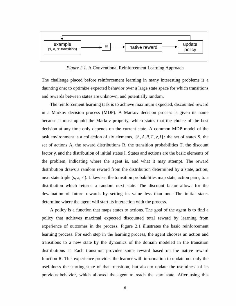
Figure 2.1. A Conventional Reinforcement Learning Approach
The challenge placed before reinforcement learning in many interesting problems is a
daunting one: to optimize expected behavior over a large state space for which transitions
and rewards between states are unknown, and potentially random.
The reinforcement learning task is to achieve maximum expected, discounted reward
in a Markov decision process (MDP). A Markov decision process is given its name
because it must uphold the Markov property, which states that the choice of the best
decision at any time only depends on the current state. A common MDP model of the
task environment is a collection of six elements, },,,,,{ ITRAS γ : the set of states S, the
set of actions A, the reward distributions R, the transition probabilities T, the discount
factorγ, and the distribution of initial states I. States and actions are the basic elements of
the problem, indicating where the agent is, and what it may attempt. The reward
distribution draws a random reward from the distribution determined by a state, action,
next state triple (s, a, s′). Likewise, the transition probabilities map state, action pairs, to a
distribution which returns a random next state. The discount factor allows for the
devaluation of future rewards by setting its value less than one. The initial states
determine where the agent will start its interaction with the process.
A policy is a function that maps states to actions. The goal of the agent is to find a
policy that achieves maximal expected discounted total reward by learning from
experience of outcomes in the process. Figure 2.1 illustrates the basic reinforcement
learning process. For each step in the learning process, the agent chooses an action and
transitions to a new state by the dynamics of the domain modeled in the transition
distributions T. Each transition provides some reward based on the native reward
function R. This experience provides the learner with information to update not only the
usefulness the starting state of that transition, but also to update the usefulness of its
previous behavior, which allowed the agent to reach the start state. After using this
example(s, a, s’ transition) R native reward
updatepolicy
7
information to update the current policy, the agent, based on its exploration strategy and
current policy, picks another action to execute.
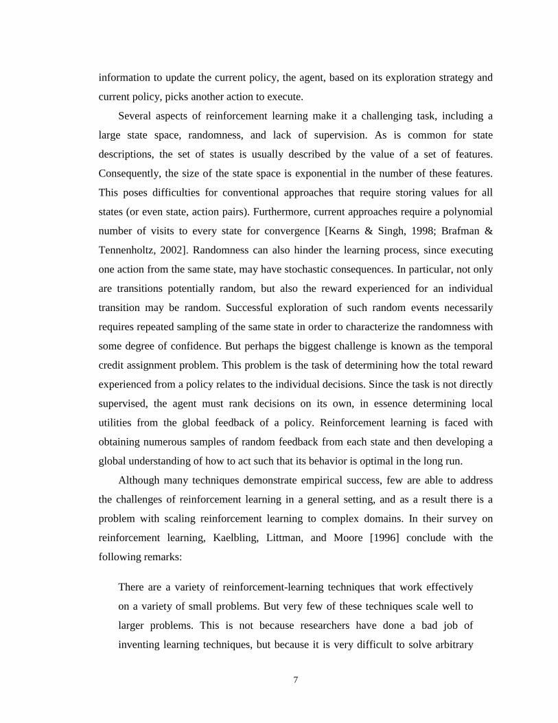
Several aspects of reinforcement learning make it a challenging task, including a
large state space, randomness, and lack of supervision. As is common for state
descriptions, the set of states is usually described by the value of a set of features.
Consequently, the size of the state space is exponential in the number of these features.
This poses difficulties for conventional approaches that require storing values for all
states (or even state, action pairs). Furthermore, current approaches require a polynomial
number of visits to every state for convergence [Kearns & Singh, 1998; Brafman &
Tennenholtz, 2002]. Randomness can also hinder the learning process, since executing
one action from the same state, may have stochastic consequences. In particular, not only
are transitions potentially random, but also the reward experienced for an individual
transition may be random. Successful exploration of such random events necessarily
requires repeated sampling of the same state in order to characterize the randomness with
some degree of confidence. But perhaps the biggest challenge is known as the temporal
credit assignment problem. This problem is the task of determining how the total reward
experienced from a policy relates to the individual decisions. Since the task is not directly
supervised, the agent must rank decisions on its own, in essence determining local
utilities from the global feedback of a policy. Reinforcement learning is faced with
obtaining numerous samples of random feedback from each state and then developing a
global understanding of how to act such that its behavior is optimal in the long run.
Although many techniques demonstrate empirical success, few are able to address
the challenges of reinforcement learning in a general setting, and as a result there is a
problem with scaling reinforcement learning to complex domains. In their survey on
reinforcement learning, Kaelbling, Littman, and Moore [1996] conclude with the
following remarks:
There are a variety of reinforcement-learning techniques that work effectively
on a variety of small problems. But very few of these techniques scale well to
larger problems. This is not because researchers have done a bad job of
inventing learning techniques, but because it is very difficult to solve arbitrary
8
problems in the general case. In order to solve highly complex problems, we
must give uptabula rasalearning techniques and begin to incorporate bias that
will give leverage to the learning process.
It is precisely for this reason that we investigate reward shaping. Shaping expresses
prior knowledge through rewards as a means to condition good behavior. Since prior
knowledge is commonly available, and reward is universal to reinforcement learning,
shaping shows promise as a general technique for solving larger tasks. But it is crucial
that we understand how it works in order to guarantee that the successes of shaping are
more than solutions to a variety of small problems. By providing a foundation of
theoretical results, we take the first steps to promote shaping as a robust method for
applying the bias that is needed to succeed in complex problems of diverse domains.
2.2 Shaping with Rewards
The technique of reward shaping works to alleviate the temporal credit assignment
problem by making the correct behavior apparent through localized advice. The localized
advice is applied via a shaping function, F, which acts similarly to the native reward
function R. On each transition, the shaping function makes some judgment on the
experience, and returns a corresponding reward value. The goal of shaping is to make use
of prior knowledge to correctly lead the agent toward good performance overall, thereby
accelerating the process of converging to an acceptable policy.
Reward shaping can be directly applied to reinforcement learning by adding the
shaping rewards to the native rewards after every transition (Figure 2.2). Consequently,
the process of shaping is equivalent to learning in a more supportive environment. The
new environment is the transformation of the native MDP to a shaped MDP with
augmented rewards. Using the notation for a Markov decision process, the native MDP
},,,,,{ ITRASM γ= is converted to the shaped MDP },,,,,{' ITFRASM γ+= . Any
conventional RL algorithm can be used on the shaped process M′, just as if it were a
separate problem. Successful shaping transforms the native process M such that the
shaped process is easier to learn, but still preserves the optimal policy of M.

9
Figure 2.2. Reinforcement Learning with Reward Shaping
2.3 Contributions
The primary contribution of this work is the first comprehensive theory on the field
of reward shaping. The main areas of interest are:
1. An analysis of the effects of reward shaping on the speed of reinforcement
learning. We conclude that the reward horizon is the important parameter that
relates the effectiveness of shaping, and prove that it has the strongest influence
on running time for a simple reinforcement learning algorithm. Furthermore,
when learning makes use of the reward horizon, it is possible to learn an
approximately optimal policy in time that does not depend on the size of the state
space, but rather on the number of states within the horizon.
2. The definition of an ideal shaping reward. We prove that opportunity value is the
ideal shaping reward in the sense that it will reduce the reward horizon to one, and
preserve the optimal solution of the native task.
3. Several practical shaping techniques to employ imperfect and imprecise prior
knowledge to approximate opportunity value. Among these are subgoal shaping
and dynamic shaping which demonstrate the potential to accelerate learning by
reducing the reward horizon with localized advice.
4. Two experimental investigations into the application of reward shaping. We
conduct experiments in a stochastic gridworld, and bipedal walking task. These
experiments validate our analytical claims and provide evidence to support the
use of our practical shaping techniques.
example(s, a, s’ transition)
R native reward
shaping reward
updatepolicy
F
10
CHAPTER3
The Reward Horizon
The capacity to adapt and learn quickly depends on accurate judgments of
performance that criticize deficient areas and offer advice of how to improve. This idea is
especially relevant for reinforcement learning (RL), where the rewards that provide
judgments can range from misleading to perfect guidance. Naturally, such a range of
possibilities impacts the ability to learn quickly. In this chapter, we define the reward
horizon, a metric that summarizes the varied inaccuracies of the judgments of individual
rewards. Because it captures the quality of the feedback of a task, the reward horizon also
describes the rate at which the process as a whole can be learned.
Policy acquisition in reinforcement learning can be viewed as solving a set of
classification learning tasks, but with several significant complications. The learning
tasks are to label each state (or state-action pair) with its utility. The primary
complications in solving this task are that the training feedback on a state classification is
ambiguous and delayed. The ambiguity is a result of the stochastic nature of the problem.
When executing the policy for a given state, both the next state and the reward
experienced may be random. A higher variance for either the next state or the reward
makes any estimate of the utility less confident. Delayed feedback [Tesauro, 1992] results
from reward schemes that separate a decision from a good estimate of its return with
several intermediate actions. For example, playing a game of backgammon with a reward
of one for winning and zero otherwise, introduces a delay between decision and
feedback. As the delay increases, the number of reachable states and potentially relevant
rewards can increase exponentially. And since utility is the maximum expected value
11
over these rewards, a reliable estimate may require exponentially more samples as the
delay increases.
We encapsulate the factors that complicate learning in the notion of the reward
horizon. The reward horizon is a measure of the number of decisions a learning agent
must make before experiencing accurate feedback. The reward horizon determines a
boundary around each state such that, given a reasonable amount of experience within the
boundary, a good action can be reliably chosen. Therefore, as the horizon shrinks, the
ambiguity and delay of the reward process must also decrease. And as these
complications are reduced, so is the difficulty of learning. In this way, we identify low
reward horizons with easy-to-learn Markov decision processes (MDPs).
3.1 A Path-Based Perspective
The reward horizon requires that the total reward within a bounded region of states
provides the same decision ordering as the global return of the process. One way to
understand this concept more formally is to cast reinforcement learning concepts into a
path-based frame work. Within a finite horizon, each path is rated by a discounted sum of
local rewards. Local utilities are the expectation of the finite path sums over the
distribution of paths resulting from applying the optimal policy. The critical property that
makes a problem easy to solve is that the local utilities reflect good performance on a
global scale. In other words, local utilities must rank their initial decisions according to
the global utilities. The transition from finite path sums, to local utilities, to global
utilities illustrates the process we use to identify the reward horizon of a MDP.
Finite path sums are the discounted total of all rewards along a bounded sequence of
transitions. In the reward shaping framework, this means using the sum of all the native
rewards from the function R, and all the shaping rewards from the function F. The
shaping function transforms the native process M, which optimizes using only R, to a
new process Mÿ, which optimizes R+F. To analyze the effectiveness of the shaping
function, we look at the discounted total return of R+F over a finite path. A path p, of
length n, is written p = (s0 a0, s1 a1, … sn), where each si is the state reached after i
actions, and ai is the action executed in state si. Each state, action, next state triple along
12
the path determines both native and shaping rewards: Ri = R(si, ai, si+1) and likewise Fi =
F(si, ai, si+1). W use R(si, ai, si+1) to denote the mean reward for the transition, rather than
random output of the corresponding reward distribution. Using this notation, we have a
compact description of finite path sums.
Definition 3.1 Thefinite path sumof a path p = (s0 a0, s1 a1, … sn) is
( )ÿ−
=
−−−
−−−
+=
++++=1
0
111
111
100100 ),,(),,(...),,(),,()(n
iii
i
nnnn
nnnn
n
FR
sasFsasRsasFsasRpS
γ
γγ
It is also useful to describe the distribution of paths driven by a given policy. A path
of length n, driven by policyπ is p = (s0 π(s0), s1 π(s1), … sn). If we consider p a random
variable drawn from all possible paths that start in state s0 and execute the policyπ for n
steps, then its distribution is writtenπ0sP . Likewise it is useful to consider the distribution
of paths that first execute some action a, and then follow policyπ. We denote such a
distribution πa,s0
P .
We can write the traditional RL utilities as the expectation of path sums over these
distributions. These utilities are the expected path sums over the distribution of paths that
executes the global optimal policy of the shaped process,*M'� . Because they are the
expected sum of an infinite (discounted) series of rewards, and thus encompass the entire
problem, we describe these utilities as global.
Definition 3.2 The global state utility for executing the global optimal policy*M'
* �=π , starting in state s, in the MDP Mÿ is
[ ] ( )��
���
�+== ÿ
∞
=∞
0~~ **)()(
iii
i
PpPpFREpSEsV
ss
γππ
Definition 3.3 The global Q-valuefor executing action a in state s, and then the
global optimal policy *M'
* �=π , in the MDP Mÿ is
[ ] ( )��
���
�+== ÿ
∞
=∞
0~~ *,
*,
)(),(i
iii
PpPpFREpSEasQ
asas
γππ
13
Notation Scope Process Description
)(sV , ),( asQ Global Shaped Utility
)(sVn , ),( asQn Local Shaped Utility
)(sV M , ),( asQM Global Native Utility
*π Global Shaped Optimal Policy*
)(' sM nπ Local Shaped Optimal Policy
*Mπ Global Native Optimal Policy
Table 3.1. Utility and Policy Notation
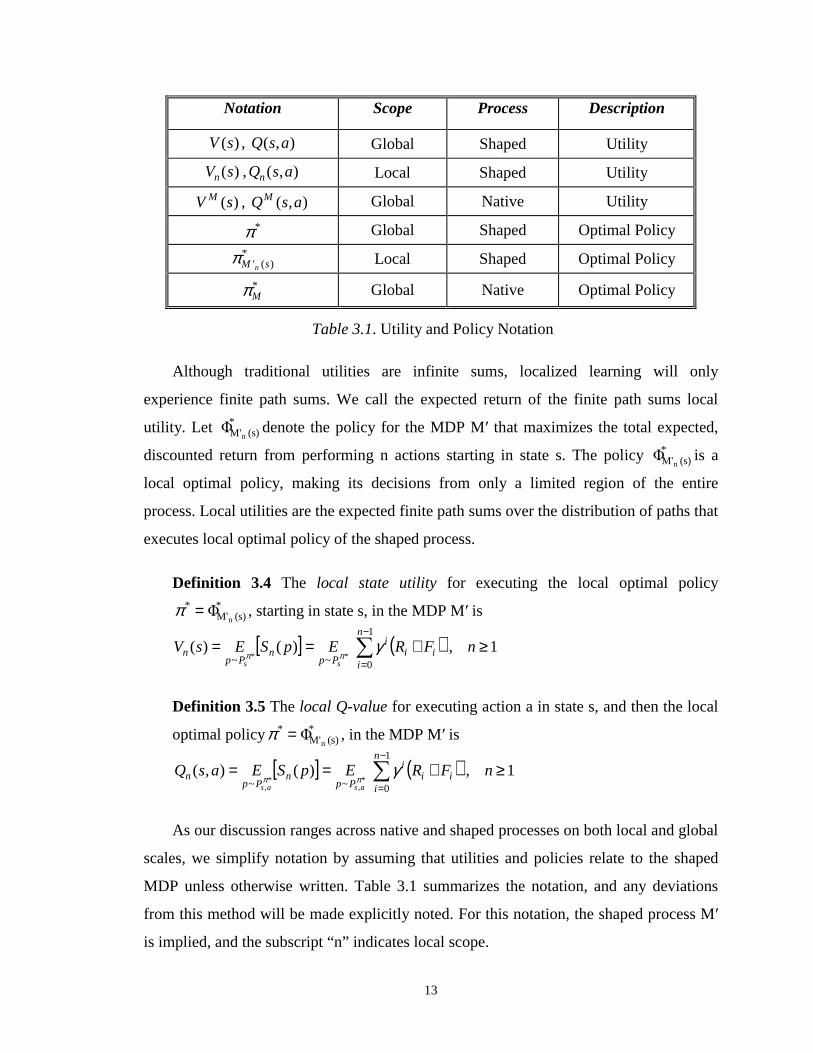
Although traditional utilities are infinite sums, localized learning will only
experience finite path sums. We call the expected return of the finite path sums local
utility. Let *(s)M'n
� denote the policy for the MDP Mÿ that maximizes the total expected,
discounted return from performing n actions starting in state s. The policy*(s)M'n
� is a
local optimal policy, making its decisions from only a limited region of the entire
process. Local utilities are the expected finite path sums over the distribution of paths that
executes local optimal policy of the shaped process.
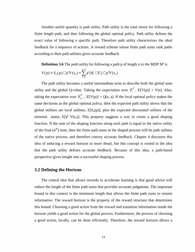
Definition 3.4 The local state utility for executing the local optimal policy*
(s)M'*
n�=π , starting in state s, in the MDP Mÿ is
[ ] ( ) 1,)()(1
0~~ **≥�
�
���
�+== ÿ
−
=nFREpSEsV
n
iii
i
Ppn
Ppn
ss
γππ
Definition 3.5 The local Q-valuefor executing action a in state s, and then the local
optimal policy *(s)M'
*n
�=π , in the MDP Mÿ is
[ ] ( ) 1,)(),(1
0~~ *,
*,
≥��
���
�+== ÿ
−
=nFREpSEasQ
n
iii
i
Ppn
Ppn
asas
γππ
As our discussion ranges across native and shaped processes on both local and global
scales, we simplify notation by assuming that utilities and policies relate to the shaped
MDP unless otherwise written. Table 3.1 summarizes the notation, and any deviations
from this method will be made explicitly noted. For this notation, the shaped process Mÿ
is implied, and the subscript “n” indicates local scope.
14
Another useful quantity is path utility. Path utility is the total return for following a
finite length path, and then following the global optimal policy. Path utility defines the
exact value of following a specific path. Therefore path utility characterizes the ideal
feedback for a sequence of actions. A reward scheme whose finite path sums rank paths
according to their path utilities gives accurate feedback.
Definition 3.6 Thepath utility for following a path p of length n in the MDP Mÿ is
)()()()()(1
0n
nn
iii
in
nn sVFRsVpSpV γγγ ++=+= ÿ
−
=
The path utility becomes a useful intermediate term to describe both the global state
utility and the global Q-value. Taking the expectation over*
sPπ , E[V(p)] = V(s). Also,
taking the expectation over*
as,Pπ , E[V(p)] = Q(s, a). If the local optimal policy makes the
same decisions as the global optimal policy, then the expected path utility shows that the
global utilities are local utilities, E[Sn(p)], plus the expected discounted utilities of the
terminal states, E[γn V(sn)]. This property suggests a way to create a good shaping
function. If the sum of the shaping function along each path is equal to the native utility
of the final (nth) state, then the finite path sums in the shaped process will be path utilities
of the native process, and therefore convey accurate feedback. Chapter 4 discusses this
idea of inducing a reward horizon in more detail, but this concept is rooted in the idea
that the path utility defines accurate feedback. Because of this idea, a path-based
perspective gives insight into a successful shaping process.
3.2 Defining the Horizon
The central idea that allows rewards to accelerate learning is that good advice will
reduce the length of the finite path sums that provides accurate judgments. The important
bound in this context is the minimum length that allows the finite path sums to remain
informative. The reward horizon is the property of the reward structure that determines
this bound. Choosing a good action from the reward and transition information inside the
horizon yields a good action for the global process. Furthermore, the process of choosing
a good action, locally, can be done efficiently. Therefore, the reward horizon allows a
15
process to be broken into local sub-problems, which focuses experience on relevant areas
and improves the learning rate.
A complete optimal policy maps every state to the action that promotes the highest
expected, discounted total reward. However, in many cases the Markov process that
results from applying the optimal policy will not visit all of the state space. Spending
time to optimize behavior for those states that are very unlikely to be reached
unnecessarily complicates the learning process. For example, a tennis player will not
spend time training how to return an opponent’s smash while facing backwards.
Although this is a possible configuration in the state space, it is hardly necessary to
optimize in order to perform well. We can describe the set of all useful states as those that
may be reached by following the optimal policy from any of the possible initial states.
This set of states is the ideal critical region for the MDP.
Definition 3.7 The ideal critical region, CR, of an MDP M, is the set of all states
that may be reached by starting in any initial state of M, and executing the optimal
policy.
The ideal critical region is another way viewing convergence to the optimal policy.
We have an optimal solution if we can (1) identify all states in the ideal critical region,
and (2) make the optimal decision for each of these states. Notice that this region can be
small in many cases. For deterministic cases, it is only the length of that path from the
initial state to the goal state, or the length of the highest return cycle. Otherwise, the CR
grows with the randomness imparted by the transition probabilities.
Our goal is to identify an approximately optimal policy, which achieves a total
expected return withinε of the optimal. Because these policies make different choices
than the optimal, they may visit a different subset of the state space when executed.
However, it is sufficient to know only one such subset. Therefore, we refer to a critical
region as a subset of the state space that is reachable from any initial state executing any
near-optimal policy.
Definition 3.8 A critical region of an MDP M, is the set of all states that may be
reached by starting in any initial state of M, and executing one near-optimal policy.
16
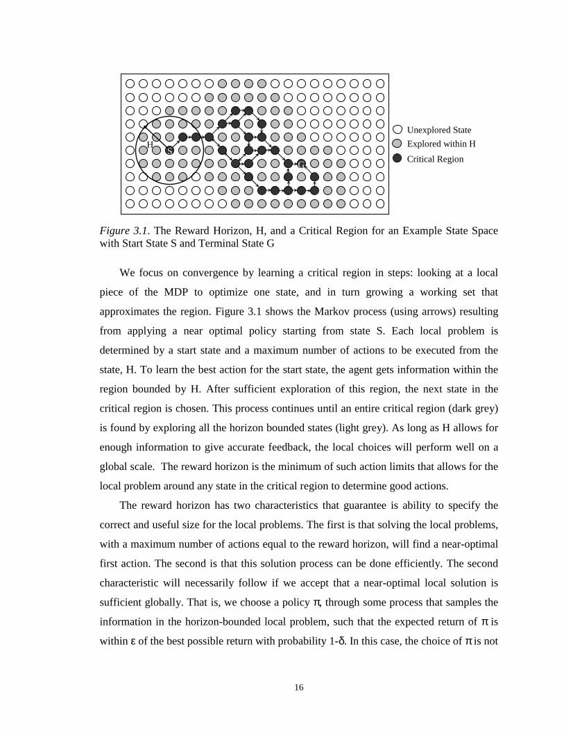
Figure 3.1. The Reward Horizon, H, and a Critical Region for an Example State Spacewith Start State S and Terminal State G
We focus on convergence by learning a critical region in steps: looking at a local
piece of the MDP to optimize one state, and in turn growing a working set that
approximates the region. Figure 3.1 shows the Markov process (using arrows) resulting
from applying a near optimal policy starting from state S. Each local problem is
determined by a start state and a maximum number of actions to be executed from the
state, H. To learn the best action for the start state, the agent gets information within the
region bounded by H. After sufficient exploration of this region, the next state in the
critical region is chosen. This process continues until an entire critical region (dark grey)
is found by exploring all the horizon bounded states (light grey). As long as H allows for
enough information to give accurate feedback, the local choices will perform well on a
global scale. The reward horizon is the minimum of such action limits that allows for the
local problem around any state in the critical region to determine good actions.
The reward horizon has two characteristics that guarantee is ability to specify the
correct and useful size for the local problems. The first is that solving the local problems,
with a maximum number of actions equal to the reward horizon, will find a near-optimal
first action. The second is that this solution process can be done efficiently. The second
characteristic will necessarily follow if we accept that a near-optimal local solution is
sufficient globally. That is, we choose a policyπ, through some process that samples the
information in the horizon-bounded local problem, such that the expected return ofπ is
within ε of the best possible return with probability 1-δ. In this case, the choice ofπ is not
Unexplored State
Explored within H
Critical Region
HS
G
17
arbitrarily hard, and independent to how close competing polices may be. This allowsπ
to be chosen efficiently, and is acceptable as long as the first action ofπ is near-optimal
globally.
Definition 3.9 A MDP M has areward horizonof H, if and only if for every state s
in a critical region of M, choosinga such that ε≤− )ˆ,()( asQsV HH with
probability δ−1 , implies ε2)ˆ,()( ≤− asQsV with probability δ21− .
The reward horizon has a simple interpretation: selecting an approximately optimal
action from the information in the region bounded by H results in an approximately
optimal return for the entire MDP. The choice to double the final approximation and
chance of failure is not significant; it simply allows for some slack in the translation of
local utilities to global utilities. The reward horizon translates good local performance to
good global performance. This property relates reducing the horizon to providing more
immediate feedback. And this localized advice, in turn, focuses exploration, making the
identification of the critical region easier, and therefore speeding convergence.
3.3 Using the Reward Horizon
We have argued that the reward horizon explains the success of shaping by
describing a minimal search boundary. This section uses knowledge of the reward
horizon to derive the amount of work needed to converge to an approximately optimal
policy. Based on this analysis, we will show that a simple algorithm can learn efficiently,
by disregarding irrelevant parts of the state space.
Any given MDP will have a reward horizon. The reward horizon may be as long as
ε-horizon time [Kearns & Singh, 1998]. Theε-horizon time is the number of steps that
the learner must take before the rest of the discounted future return can be at mostε. In
this case, there is no locality to the rewards; all information is delayed until the end. A
reward horizon equal to theε-horizon time means that no algorithm could pick the best
action until it sees everything in the problem that could have a significant impact on the
total return. On the other extreme, the reward horizon may be one, meaning that the
feedback from a single transition is enough to determine the best decision. More
18
commonly, we expect that shaping can transform a reward structure with a large horizon
to one with a lesser value. This ability of shaping with prior knowledge motivates our
research on the reward horizon.
We wish to investigate the effects of learning while exploiting the reward horizon.
The approach we propose is to grow a set of known states that will eventually include
enough states to reliably conclude that the policy computed from these states is very close
to the optimal. In essence, we learn a critical region. Marking a state known indicates that
we have sufficient information to reliably decide on the best action for that state. We
develop known states by solving the relevant local problems bounded by the reward
horizon. Growing the set is a forward-chaining operation; as early actions become fixed,
later elements in the critical region are visited more frequently and subsequently become
known. Once enough states are known, we continue to follow the current policy until
enough evidence is gathered to support termination with a good policy.
Next, we present a learning algorithm that specifies this approach. The remainder of
this section formally specifies and provides an analysis of this algorithm that leads to its
running time. Our analysis discusses in detail how to make a state known, how to learn a
sufficient portion of a critical region, and how to conclude that the algorithm has
converged to an approximately optimal solution.
3.3.1 THE HORIZON _LEARN ALGORITHM
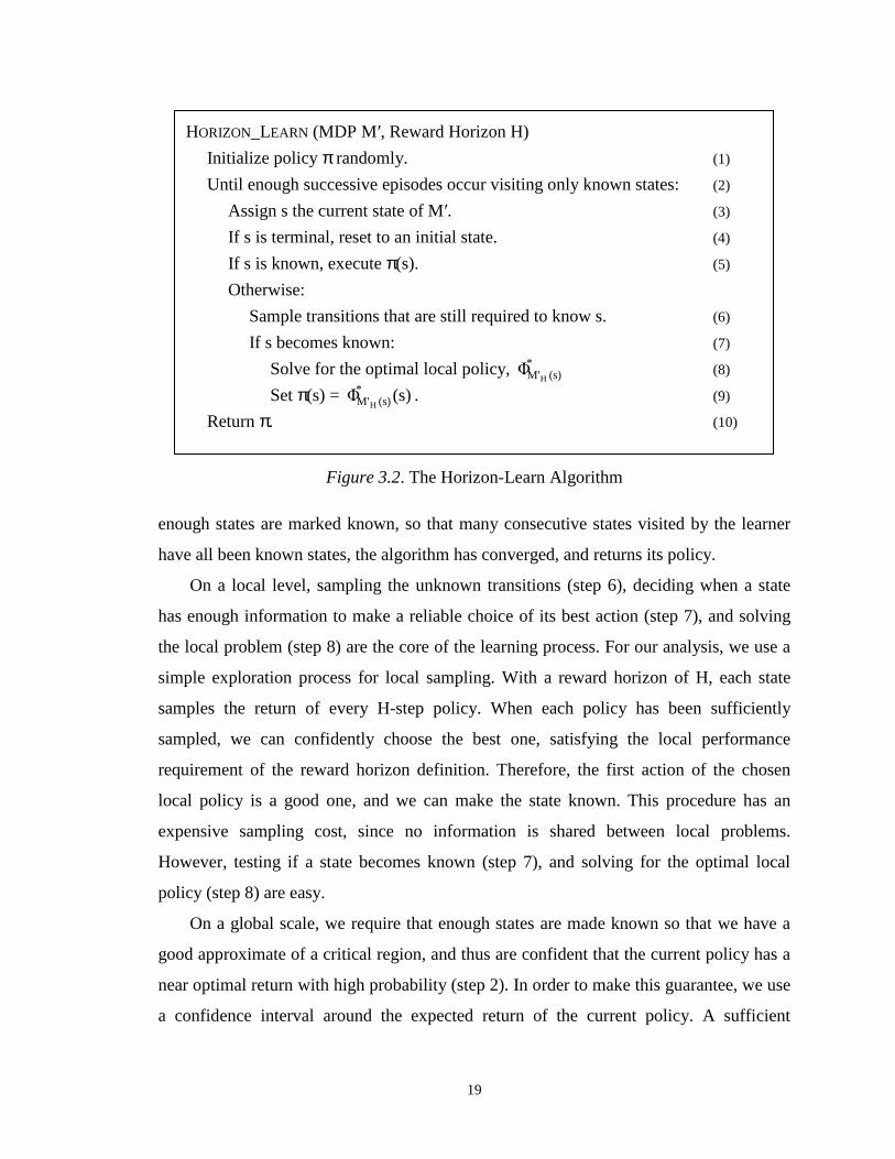
The Horizon-Learn algorithm (Figure 3.2) outlines a general procedure to make use
of the reward horizon for reinforcement learning. The basic process is to estimate the best
action for each state, and mark them known, based on sampling the information in the
local horizon-bounded problem. When enough samples of the transition and reward
structure are experienced, the local problem around a state is solved, and the state
becomes known. As more states become known, the set of all known states begins to
approximate the critical region of the process for some near-optimal policy. Every time a
state is marked known, it will execute the action it has decided is best. Because these
actions are near-optimal by definition of the reward horizon, future exploration is focused
on important states. This efficient use of experience promotes accelerated learning. Once
19
Figure 3.2. The Horizon-Learn Algorithm
enough states are marked known, so that many consecutive states visited by the learner
have all been known states, the algorithm has converged, and returns its policy.
On a local level, sampling the unknown transitions (step 6), deciding when a state
has enough information to make a reliable choice of its best action (step 7), and solving
the local problem (step 8) are the core of the learning process. For our analysis, we use a
simple exploration process for local sampling. With a reward horizon of H, each state
samples the return of every H-step policy. When each policy has been sufficiently
sampled, we can confidently choose the best one, satisfying the local performance
requirement of the reward horizon definition. Therefore, the first action of the chosen
local policy is a good one, and we can make the state known. This procedure has an
expensive sampling cost, since no information is shared between local problems.
However, testing if a state becomes known (step 7), and solving for the optimal local
policy (step 8) are easy.
On a global scale, we require that enough states are made known so that we have a
good approximate of a critical region, and thus are confident that the current policy has a
near optimal return with high probability (step 2). In order to make this guarantee, we use
a confidence interval around the expected return of the current policy. A sufficient
HORIZON_LEARN (MDP Mÿ, Reward Horizon H)
Initialize policyπ randomly. (1)
Until enough successive episodes occur visiting only known states:(2)
Assign s the current state of Mÿ. (3)
If s is terminal, reset to an initial state. (4)
If s is known, executeπ(s). (5)
Otherwise:
Sample transitions that are still required to know s. (6)
If s becomes known: (7)
Solve for the optimal local policy, *(s)M'H
� (8)
Setπ(s) = (s)�*(s)M'H
. (9)
Returnπ. (10)
20
condition that implies near optimal performance is to repeatedly visit states that the
current policy has already optimized, gaining confidence from each episode that visits
only known states. So once the number of consecutive known states is high enough, the
algorithm terminates with near-optimal performance. The total time for this to occur is
the time it takes to acquire a good approximation of the critical region plus the time it
takes to guarantee that performance using the optimized critical region is acceptable.
3.3.2 EXPLORATION AND RECOGNIZING KNOWN STATES
A known state is a state for which we believe we have found an approximately
optimal action with some level of confidence. States are marked known by local problem
exploration and solving, steps 6-8 of Horizon-Learn. Gaining experience in each local
problem eventually allows for the confident choice of a good local action. When each
local problem is bounded by the reward horizon, by definition, the local action is also a
good global action. After a state becomes known, its successor states enter the critical
region, and the process of creating known states continues forward.
We outline a simple, policy-based procedure for solving local problems. Namely, we
will acquire a number of samples of every policy within the region around a state
bounded by the horizon, and choose the policy with the highest sample mean. Because
the true mean of a policy is estimated from experience, it is not possible to know the best
action with zero probability of error. We require a sampling method that will correctly
choose the optimal policy within a reasonable chance of error. The following results
derive such a method.
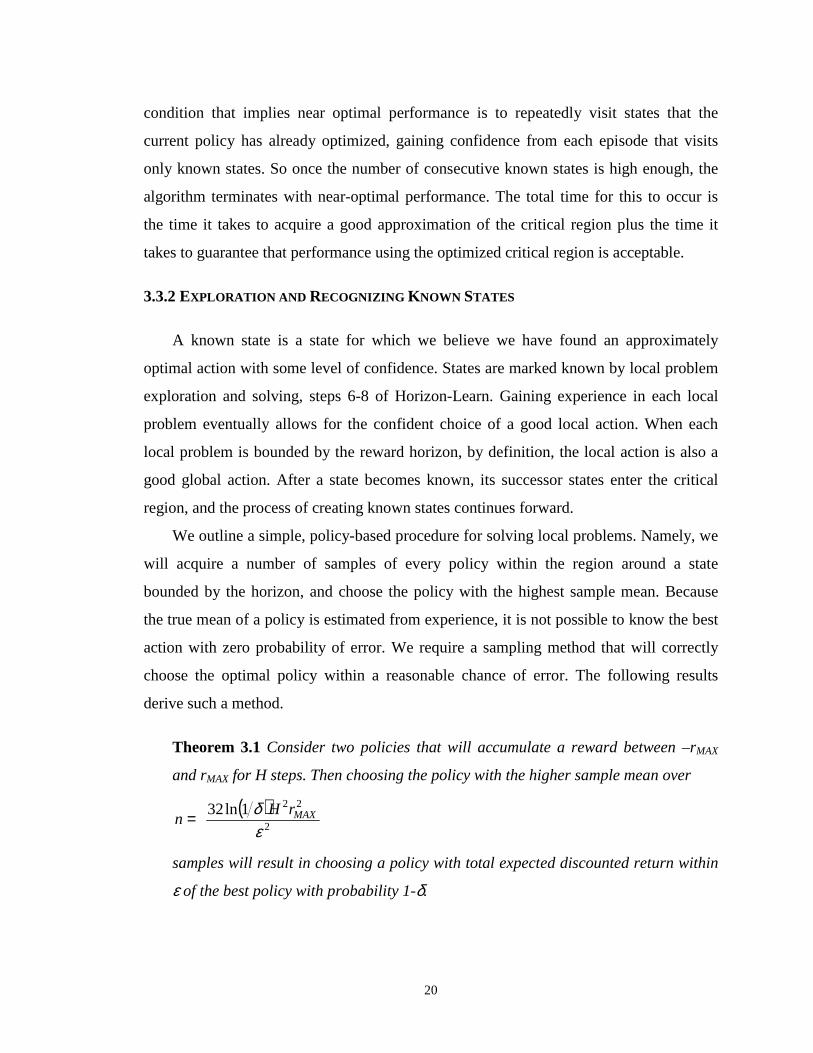
Theorem 3.1Consider two policies that will accumulate a reward between –rMAX
and rMAX for H steps. Then choosing the policy with the higher sample mean over
( )��
���
�= 2
221ln32
εδ MAXrH
n
samples will result in choosing a policy with total expected discounted return within
ε of the best policy with probability 1-δ.
21
Proof. We apply a version the Hoeffding Inequality. Given random variablesiX ,
such that 1≤iX , and ( ) 0=iXE ,
( )2expPr 2
1
ntntXn
ii −≤�
�
���
�≥ÿ
=
Let 1iR and 2
iR be the random variables describing the total expected discounted
return of policies one and two during the ith trial. Let the mean of the return of the
policies on any trial be 1µ and 2µ respectively. Without loss of generality, let
εµµ ≥− 21 . (Choosing policy one as the better policy is a naming convention, and if
εµµ <− 21 , the theorem is already proven.) Let 21iii RRD −= .
Then,( )
MAX
ii Hr
DY
421 −−= µµ
is a random variable with 1≤iY , and ( ) 0=iYE .
By Hoeffding’s Inequality,
( )2expPr 2
1
ntntYn
ii −≤�
�
���
�≥ÿ
=
( ) ( )2exp4Pr 221
1
ntntHrnD MAX
n
ii −≤�
�
���
�+−−≥−ÿ
=µµ
( )[ ] ( )2exp4Pr 221 nttHrD MAX −≤−−≤ µµ
Let( )
MAXHrt
421 µµ −= .
[ ] [ ] ( )���
����
� −−≤≤=≤ 22
221
2132
expPr0PrMAXrH
nRRD
µµ
The probabilityD is less than zero is the probability we make a mistake, and choose
policy two because its sample mean was higher. We require this chance to be less
thanδ.
( ) δµµ ≤���
����
� −− 22
221
32exp
MAXrH
n
( ) ( )δµµ1ln
32 22
221 ≥−
MAXrH
n
22
( )( )221
221ln32
µµδ−
≥ MAXrHn and since εµµ ≥− 21 ,
( )2
221ln32
εδ MAXrH
n ≥ �
Theorem 3.1 gives the number of samples required to guarantee that the policy
corresponding to the higher sample mean of two policies will perform well. We can
readily generalize these results to the comparison of several policies. With multiple
policies, an error is made if any policy with poor performance is chosen. The following
bounds the number of samples needed for the worst case, when every possible competitor
policy is a poor choice, just below the threshold for being acceptable.
Theorem 3.2Consider m policies that will accumulate a reward between –rMAX and
rMAX for H steps. Then choosing the policy with the higher sample mean over
( )���
�
���
�=
−
2
221ln32
εδ MAX
m rHn
samples will result in choosing a policy with total expected discounted return within
ε of the best policy with probability 1-δ.
Proof. Let R1… Rm be the random variables describing the total expected discounted
return of policies one to m, respectively. Without loss of generality, let the policy
with the highest return be policy one. Letp~ = Pr( 1R < 2R OR 1R < 3R … OR
1R < mR ) where each iR for i = 2 to m has a mean iµ such that εµµ ≥− i1 or
i1 RR < is excluded fromp~ . Then p~ is the chance of error by picking a policy with
return more thanε below the best policy, and may be at mostδ. We can boundp~
with the sum of the probability of the individual comparisons. Let
( )ÿ <=i
i1 RRPrp , for each iR in p~ .
Then pp~ ≤ , since the events 1R < iR are not mutually exclusive.
For each policy, calculate the sample mean from( )
���
�
���
�=
−
2
221ln32
εδ MAX
m rHn .
Then either εµµ ≥− i1 and ( )≤< i1 RRPr 1−mδ by Theorem 3.1, or the term
( )i1 RRPr < is excluded from pˆ (because it is not an error). Therefore, δ≤≤ pp~ . �
23
Theorem 3.2 provides an effective sampling method if the number of policies that
are being compared is known. We provide an upper bound to the number of policies to
apply Theorem 3.2 more generally. In order to count the maximum number of policies
within a given horizon, we must characterize the randomness of the domain. To this end,
we define a branching factor b, the maximum number of successor states for any state-
action. The maximum number of policies is then bH-1|A|H, allowing for |A| decisions at
the start state, and b|A| decisions branching from each step in the policy up to H. Using
this bound, we can define the maximum number of visits to a state before it becomes
known.
Corollary 3.3 Let Mÿ be a MDP with horizon H and rewards with absolute value
bounded by rMAX. Then a state s in Mÿ becomes known, choosing an action withinε
of the best H step return with probability 1-δ, after sampling every local policy
evenly, with at most
( ) ���
����
�=
−−
δεδε
HH
MAXHH
knownAb
rHAbn||
ln1
||321
2221,
visits to the state s.
Corollary 3.3 is the result of Theorem 3.2 with m = bH-1|A|H, multiplied by the
maximum number of local polices. This corollary serves as the formal definition of
known states, which implements the steps 6-8 of Horizon-Learn (Figure 3.2) using direct
policy-based sampling.
3.3.3 LEARNING A CRITICAL REGION
On a global scale, the major task of learning under our framework is identifying a
sufficient portion of a critical region such that we meet a high level of performance with a
small chance of failure. We might think of learning the entire CR. In this case, we would
achieve near optimal return without ever reaching a state that is unknown. The drawback
is that we must learn every state, regardless of how improbable, or unrewarding. In fact,
the difficulty in reaching unknown states in the CR plays a major role in the time it takes
24
to learn. In order to reduce the number of unlikely states to learn, we choose to learn a
subset of the critical region.
The idea of learning a critical region is to gather a number of states in the CR
through diligent exploration, such that our chance of visiting only known states is high.
Once this probability is high enough, we will experience many applications of the current
policy which visit no unknown states. In other words, we have a policy which, although
not guaranteed for every state, executes near-optimal actions for all of the most common
paths. Each time an execution introduces no unknown states, we gain evidence to bound
the expected return of the current policy. If there is sufficient number of such
observations, we can conclude that the current policy is very likely to be approximately
optimal.
The performance criterion we guarantee for a policy is the initial state return. The
following results ensure that the total expected discounted return over the random initial
states determined by the MDP is approximately optimal with high confidence.
Definition 3.10 The initial state returnof a policy π , πµ , in a MDP M with initial
state distribution I, is the expected utility of executingπ from initial states,
( )��
���
�= ∞ )(~~
pSEEsPpIs π
πµ .
The initial state return measures how well a policy will perform on average during an
episode. Each episode is a period starting from some initial state, until the process is reset
to a new initial state drawn from I. Aside from explicitly episodic domains, we emphasize
that initial state return can apply to any domain with a process that makes one sequence
of actions independent of another. We refer to such a process as a reset. For example, if
applying π to an MDP M yields an ergodic Markov chain, and the initial state
distribution of M is the stationary distribution of the ergodic process, then a long enough
sequence of actions will act as a reset. The cost of the reset is the number of actions it
takes to reach the stationary distribution. On the other hand, a MDP that explicitly draws
a next state from the distribution I after reaching a terminal state, resets with no actions,
and has a cost of zero. A more general case is that some mechanism is able to reach any
desired initial state within some polynomial time reset cost. In this case, an episode is the
25
process of approaching the total discounted return of an initial state by executingπ , then
drawing a new initial state from I, and using the reset mechanism to reach that state.
One way to estimate the total return of discounted rewards is to sample the return for
a number of steps equal to theε-horizon time. [Kearns & Singh, 1998]. Theε-horizon
time is the number of actions after which the total discounted future return can be at most
ε. The following definition shows how theε-horizon time can be computed from the
properties of a given MDP.
Definition 3.10 The ε-horizon time, T, of a MDP with discount factorγ and
maximum reward rMAX is ( ) ( )γγε1
)1( lnln −≥ MAXrT .
We gain confidence in the current policy by sampling its initial state return over
many episodes. Each episode samples the initial state return ofπ for T actions, πTR , and
then applies the reset mechanism. Repeating this sampling process determines a
confidence interval for πµT , the mean initial state return executing T actions ofπ .
The following theorems define how many episodes are needed until we are sure that
the initial state return from the current policy (and critical region approximation) is near
optimal. This establishes the test for terminating the main loop of the Horizon-Learn
algorithm (step 2). Theorems 3.4 and 3.5 operate in a MDP M, with discount factorγ, and
rewards between –rMAX and rMAX.
Theorem 3.4Let πTR be the sample mean of ( ) ( ) �����
� −= −
2
51122ln50 ε
γεδMAXrn samples of
the initial state return for executing T actions ofπ , where T is the 5/ε -horizon
time. Then, the T-step initial state return forπ has the confidence interval
[ ] δεµε πππ −≥+≤≤− 15/5/Pr TTT RR .
Proof. We use the general form of the Hoeffding Inequality.
( )[ ] ( ) ���
����
�−−≤−≤ ÿ
=
n
iii abtntXXE
1
2222expPr and
( )[ ] ( ) ���
����
�−−≤+≥ ÿ
=
n
iii abtntXXE
1
2222expPr
with each iX independent and iii bXa ≤≤ .
26
We have each πTR independent, because they are from different episodes, and
5151ε
γπε
γ −≤≤+ −−− MAXMAX r
Tr R by the definition of the 5/ε -horizon time. Therefore,
( ) ( )2511
2 4 εγ −=− −
=ÿ MAXrn
iii nab , with
( )5/5/Pr εµε πππ −≤≤+ TTT RR ≤ ( ) ����
�� −− −
2
512 50exp ε
γε MAXrn .
We divide the chance of excluding the mean from the confidence interval evenly
above and below, so that
( ) 2/50exp2
512 δε ε
γ ≤����
�� −− −
MAXrn . Solving for n, ( ) ( )251122ln50 ε
γεδ −≥ −MAXrn .
So with n sufficiently large, ( )5/Pr εµ ππ −≤ TT R and ( )5/Pr εµ ππ +≥ TT R are each less
than 2/δ . �
A confidence interval alone is not enough to guarantee near optimal performance. It
must also be the case that the confidence interval is in a region with good performance.
We need to show that the initial state return for the optimal policy is very likely to be
close to the confidence interval for the performance of the current policy. If the current
policy samples its initial state return, and finds only known states, the following theorem
demonstrates that it will be approximately optimal with high probability.
Theorem 3.5Let π be a policy visiting ( ) ( ) ������ −= −
2
51122ln50 ε
γεδMAXrn episodes of only
known states. Then for an 5/ε -horizon time T, if each known state s satisfies
TssQsVγγεπ
−−≤−
1
15))(,()( , then the initial state return ofπ is within ε of the optimal
return with probability δ−1 .
Proof. Since we have visited only known states, there exists some policyπ that
executes the same actions asπ for the known states, and has its mean T-step return
within 5/ε of the optimal. That is, let )()(ˆ ss ππ = on known states, and
)()(ˆ * ss ππ = otherwise. Then the worst return forπ visits T known states, so that
51
15
1
0
ˆ* εγγεγµµ ππ =
−−≤− ÿ
−
=T
T
i
iTT
27
Becauseπ executes the same actions asπ in known states, and each episode has
visited only known states, the confidence interval of Theorem 3.4 also applies toπµ ˆT .
Using these properties ofπ we have
( ) 2/5/Pr ˆ δεµ ππ ≤+≥ TT R
( ) 2/5/5/Pr * δεεµ ππ ≤+≥− TT R
( ) 2/5/2Pr * δεµ ππ ≤+≥ TT R
Recall from Theorem 3.4, we also know( ) 2/5/Pr δεµ ππ ≤−≤ TT R . Therefore, given
the n observed T-step initial state returns, 5/3* εµµ ππ ≤− TT with probability δ−1 .
And because T is the 5/ε -horizon time, 5/** εµµ ππ −≥T and 5/εµµ ππ +≤T . Then
we have that ( ) 5/35/5/* εεµεµ ππ ≤+−− , and thus εµµ ππ ≤−* with probability
δ−1 . �
Theorems 3.4 and 3.5 outline the number of episodes visiting only known states
needed to verify that a policy is near optimal. To complete this analysis, we need to
consider the chance of failure due to assuming a state is known, when in fact it makes a
bad choice (theδ in δε ,knownn ). If π visits m distinct states each with aδk chance of
mistakenly making a state known, then the overall chance of failure is increased by at
most mδk.
Corollary 3.6 Let )1(5)1(
1
15 γε
γεγγεε −−
−−− ==
MAX
MAXT r
rk and let each known state result from
kkknownn δε , experiences of that state. If a policy π visits only known states for
( ) ( )25112,
min 2ln50 εγεδ
δε −≥ −MAX
t
t raltern consecutive episodes, for a total of m distinct known
states, then the initial state return ofπ is within ε of the optimal with probability at
least kt mδδ −−1 .
We would like to determine a subset of the critical region such that we can reach the
termination condition in Corollary 3.6. However, this is possible for any nonempty subset
that contains a complete path. To specify an approximate critical region, we need another
parameter,α. This parameter denotes the probability that the next nterminal episodes will
visit only known states – the chance of immediate termination with a near-optimal policy.
28
Definition 3.11 The approximate critical region, CRα, is any subset of the critical
region such that the probability of visiting only its elements is at leastterminal1 nα on
any given episode, executing a policy which knows near-optimal actions for every
element.
The notion ofα is an artificial one; we are not interested in specifying it, but rather
we use it to illustrate the amount of approximation that will occur. Rather than try to
identify a goodα prior to learning, we will continually add to the approximate critical
region until termination. This idea will automatically determine an appropriateα. If
several states in the critical region are very unlikely, we will tend toward a lower alpha. If
most states are easily explored, alpha will tend to be close to one.
3.3.4 REACHING CONVERGENCE
We have analyzed the local procedure of making states known and the global system
to detect convergence. The final part of our analysis is to count the number of episodes
that are needed for both to occur. The local process must meet the condition of Corollary
3.3 for a sufficient number of states to create the approximate critical region. Next, we
must gain confidence in the policy created by optimizing the approximate critical region.
This requires meeting the termination condition of Corollary 3.6.
Theorem 3.7Let CRα be a subset of the critical region with size |CRα| and let p
denote the probability of reaching the least probable state within CRα . Then, with
probability 1-δ, every state in CRα becomes known in ( )||1 1||
α
δα CRlocal FCRn −⋅= −
episodes. F is the cumulative distribution function for the negative binomial
distribution with kkknownn δε , successes and probability of success p.
Proof. The number of episodes for the least probable state to become known, t, is a
negative binomial random variable with kkknownn δε , number of successes, and probability
of success equal to p. For t, a success is simply a visit to that state. The chance of
failure is the probability that a given state is not visited enough (kkknownn δε , times). The
least probable state becomes known in ( )||1 1
α
δCRMAX Ft −= − with || α
δCR chance of
error. Since all other states are more probable,MAXt represents an upper bound for
29
the number of episodes to learn any state in the approximate critical region. Thus,
|CRα| MAXt episodes must make all the required states known with acceptable
probability. �
Theorem 3.8 Let CRα be an approximate critical region in which all states are
known, and the probability to experience nterminal successive episodes staying only
within CRα is α. Then, nterminal successive episodes staying only within CRα will
occur with probability 1-δ in ( )δ−⋅= − 11min Gnn alterglobal episodes. G is the
cumulative distribution function for the geometric distribution withα probability of
success.
Proof. Let one trial be a sequence of nterminal episodes. A trial is successful if it visits
only known states. The number of trials for a success is a geometric random variable
with chance of successα. We bound the number of trials with the acceptable chance
of error,δ, and multiply by the length of a trial to obtain the stated result. �
Theorems 3.7 and 3.8 show that the total work to reach convergence is globallocal nn +
episodes. Convergence will be near optimal if the approximation errorε and total chance
of failure δ are divided appropriately. The approximation error will be divided as
suggested in the Corollary 3.6; each state gets a fraction of the total error
)1(5)1(
1
15 γε
γεγγεε −−
−−− ==
MAX
MAXT r
rk . The total chance of failure is also divided among its various
potential causes. The chance that any state does not find a good action in the time given
to given for a state to become known is .||4/ αδδ CRk = The chance of termination
without being within ε of optimal (the confidence interval around the initial state
performance was erroneous) is .4/δδ =t The chance that any state in the approximate
critical region is not made known within the given time is ||4/ αδδ CRl = . The chance
that the algorithm does not terminate within the given time, once the approximate critical
region has been learned is .4/δδ =g
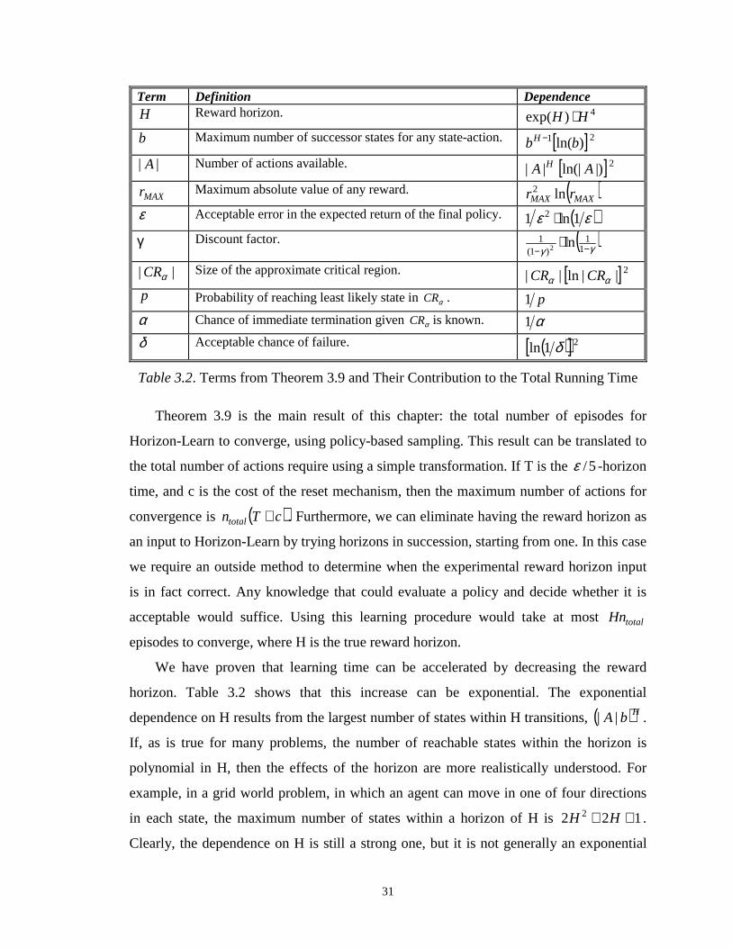
With this notation, we consolidate our results and derive the total number of episodes
for the learning process. Table 3.2 explains all the parameters of Theorem 3.9 and the
relevant terms from our previous results. Each parameter is given with its highest order
term showing its contribution to the total running time.
30
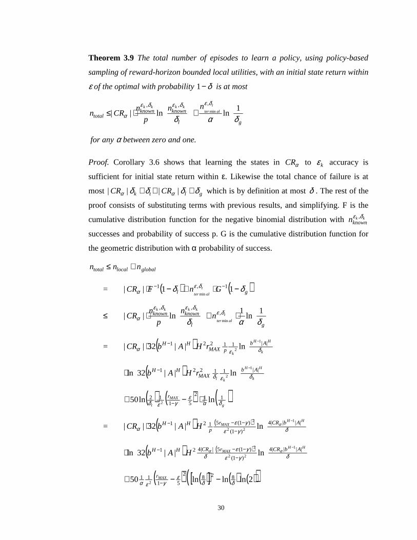
Theorem 3.9 The total number of episodes to learn a policy, using policy-based
sampling of reward-horizon bounded local utilities, with an initial state return within
ε of the optimal with probability δ−1 is at most
���
����
�+���
����
�⋅≤
gl
knownknowntotal
t
alterkkkk nn
p
nCRn
δαδ
δεδεδε
α1
lnln||,,,
min
for anyα between zero and one.
Proof. Corollary 3.6 shows that learning the states in αCR to kε accuracy is
sufficient for initial state return withinε. Likewise the total chance of failure is at
most gltk CRCR δδδδ αα +++ |||| which is by definition at mostδ . The rest of the
proof consists of substituting terms with previous results, and simplifying. F is the
cumulative distribution function for the negative binomial distribution with kkknownn δε ,
successes and probability of success p. G is the cumulative distribution function for
the geometric distribution withα probability of success.
globallocaltotal nnn +≤
= ( ) ( )gl GnFCR t
alterδδ δε
α −⋅+−⋅ −− 11|| 1,1min
≤ ���
����
�⋅+��
�
����
�⋅
gl
knownknown t
alter
kkkk
nn
p
nCR
δαδδε
δεδε
α1
ln1
ln|| ,,,
min
= ( ) ����
��⋅
−−k
HH
k
AbpMAX
HH rHAbCR δεα||11221 1
2 ln||32||
( ) ����
�� �
���
��⋅
−−k
HH
kl
AbMAX
HH rHAb δεδ||11221 1
2 ln||32ln
( ) ( ) ( )g
MAX
t
rδα
εγεδ
112
5112 lnln50 2 ⋅−+ −
= ( ) ( ) ����
��⋅
−
−−−−
δγεγε
αα
HHMAX AbCRr
pHH HAbCR ||||4
)1(
)1(51211
22
2
ln||32||
( ) ( )����
�� �
���
��⋅
−
−−−−
δγεγε
δαα
HHMAX AbCRrCRHH HAb ||||4
)1(
)1(5||421 1
22
2
ln||32ln
( ) ( )[ ] ( ) ( )( )2lnlnln50 8282
51112 δδ
εγεα −−+ −
MAXr �
31
Term Definition DependenceH Reward horizon. 4)exp( HH ⋅b Maximum number of successor states for any state-action. [ ]21 )ln(bbH −
|| A Number of actions available. [ ]2|)ln(||| AA H
MAXr Maximum absolute value of any reward. ( )MAXMAX rr ln2
ε Acceptable error in the expected return of the final policy. ( )εε 1ln1 2 ⋅γ Discount factor. ( )γγ −−
⋅ 11
)1(1 ln2
|| αCR Size of the approximate critical region. [ ]2||ln|| αα CRCR
p Probability of reaching least likely state in αCR . p1
α Chance of immediate termination given αCR is known. α1
δ Acceptable chance of failure. ( )[ ]21ln δ
Table 3.2. Terms from Theorem 3.9 and Their Contribution to the Total Running Time
Theorem 3.9 is the main result of this chapter: the total number of episodes for
Horizon-Learn to converge, using policy-based sampling. This result can be translated to
the total number of actions require using a simple transformation. If T is the5/ε -horizon
time, and c is the cost of the reset mechanism, then the maximum number of actions for
convergence is ( )cTntotal + . Furthermore, we can eliminate having the reward horizon as
an input to Horizon-Learn by trying horizons in succession, starting from one. In this case
we require an outside method to determine when the experimental reward horizon input
is in fact correct. Any knowledge that could evaluate a policy and decide whether it is
acceptable would suffice. Using this learning procedure would take at mosttotalHn
episodes to converge, where H is the true reward horizon.
We have proven that learning time can be accelerated by decreasing the reward
horizon. Table 3.2 shows that this increase can be exponential. The exponential
dependence on H results from the largest number of states within H transitions,( )HbA || .
If, as is true for many problems, the number of reachable states within the horizon is
polynomial in H, then the effects of the horizon are more realistically understood. For
example, in a grid world problem, in which an agent can move in one of four directions
in each state, the maximum number of states within a horizon of H is 122 2 ++ HH .
Clearly, the dependence on H is still a strong one, but it is not generally an exponential
32
one. For these types of situations, a learning algorithm that samples state information,
rather than policies, could learn in polynomial time, although the task of identifying
known states would be more complicated. The fundamental idea from Theorem 3.9 is
that the reward horizon dominates the running time of Horizon-Learn.
Aside from the dependence on the reward horizon, the learning time is polynomial in
its parameters, and does not depend on the size of the state space. The most demanding
parameters areb and || A , which are polynomial in the reward horizon. Every other
parameter has a dependence that is less than cubic. In particular, the learning time of
Horizon-Learn is not even quadratic in the size of the approximate critical region. This
means that whenever the number of states that a policy must see to have a good initial
state return is less than the entire state space, Horizon-Learn will learn faster than other
algorithms that must visit every state. In other words, Horizon-Learn is able to leverage
the knowledge of a reward horizon to ignore (potentially large) irrelevant regions of the
state space, to promote focused learning, efficient exploration, and faster learning.
33
CHAPTER4
Inducing a Reward Horizon
Shaping rewards can improve reinforcement learning rates by reducing the reward
horizon of a MDP. Reducing the horizon makes the delay between an action decision and
the reliable evidence of the decision’s utility shorter. Because the advice is more
immediate, the learning agent has the potential to ignore parts of the state space during its
exploration. Overall, such focused training experience allows for faster learning and
scalability to larger domains. The reward horizon defines a search radius such that the
information within the radius is enough to pick an action that is near optimal for the
entire process. In this chapter, we investigate how reward shaping can promote a minimal
search radius, and therefore a low reward horizon and faster learning.
Of primary interest are those shaping functions for which locally approximate
optimal actions in the shaped process are globally optimal in the native process. This is
the idea of inducing a reward horizon. A shaping function that induces a reward horizon
not only localizes the problem, but also retains high performance in the original task.
Preserving the optimal is not a trivial task. For example, it is very easy to foster a low
horizon by selecting any action at random and giving it a very large reward. Such an
action is both locally and globally optimal in the shaped process, because it receives a
large artificial reward. But reward shaping of this kind is uninteresting. We require
reward shaping to accelerate learning while maintaining the meaning of optimality that
the native task defines.
Ng, Harada, and Russell [1999] suggest a way to preserve the optimal policy through
potential-based shaping functions. By using a potential function over all states, they
34
prove that rewards computed as the difference of state potentials as rewards will not alter
the optimal policy of the native task. The best policy of the shaped process Mÿ must also
be the best policy of the native process M. This result, while powerful, does not describe
how shaping can accelerate learning.
Opportunity value, a difference between state utilities on a transition, combines the
ideas of preserving the optimal through potential-based shaping with reducing the reward
horizon for faster learning. Because it both accelerates learning and preserves the
optimal, opportunity value serves as insight into how successful shaping works to induce
a reward horizon. In fact, we demonstrate that scaled opportunity value is the ideal
shaping reward, in that it induces a reward horizon of one. Opportunity value guarantees
that shaping can reduce the reward horizon of any nontrivial problem, and provides an
ideal model for successful reward shaping.
4.1 Inducing a Reward Horizon
While a low reward horizon increases the locality of the rewards in a process, the
concept of inducing a reward horizon implies both increasing locality and preserving the
optimal. The goal of shaping is to optimize the native task more quickly. Unfortunately,
learning quickly and optimizing the native task are often at odds. While many types of
poor feedback can learn a bad solution quickly, only meaningful advice can teach the
correct concept. Therefore, it is important that any successful shaping technique not only
reduce the reward horizon, but also remain relevant to the native task. This is the idea of
inducing a reward horizon.
Definition 4.1 Let F be a shaping function that transforms a native MDP M to a
shaped MDP Mÿ. F induces a reward horizonof H, if and only if for every state s in
a critical region of Mÿ, choosinga such that ε≤− )ˆ,()( asQsV HH with probability
δ−1 , implies ε2)ˆ,()( ≤− asQsV MM with probability δ21− .
This definition is similar to the reward horizon, except that for inducing a reward
horizon, local optimality implies global optimality in the native process. When an action
is near the best of all its local competitors, the difference between the optimal local utility
35
and its local utility is small, ε≤− )ˆ,()( asQsV HH . If this local action works well globally
in the shaped process, we have a reward horizon. If the local action works well globally
in the native process, the difference between the optimal global native utility and the
global native Q-value is small, ε2)ˆ,()( ≤− asQsV MM . When this occurs, reward shaping
has induced a reward horizon.
The goal of reward shaping is to induce a low reward horizon. Successful shaping
drives the reward horizon lower by creating a shaping function that in some way judges a
course of action more immediately than the underlying problem. In other words, shaping
should cause the finite path sums, )( pSn , to rank paths nearly the same as the native path
utility, )( pV M . With such a ranking, accurate feedback is presented to the learner after at
most n actions. This allows for the speedup of a reward horizon of n, in addition to the
optimality provided by making decisions based on a native utility-based feedback.
4.2 Opportunity Value
A successful shaping function adds information that will cause the path return to
rank the path according to its native utility. A quantity that upholds this ranking property
is the opportunity value.
Definition 4.2 The opportunity valuefor a transition in the native MDP M, is the
difference of the final and initial state utilities, ).()'()',,( sVsVsasOPV MM −= γ
The opportunity value describes the change in return from moving to a new state,
given the current state. This quantity is suggested by the experimentation of Ng, Harada,
and Russell [1999]. We now analyze opportunity value in the context of the reward
horizon in order to demonstrate analytically how it causes speedup. Opportunity value
represents the additional information that is needed to judge a transition locally. If we
view reward as the metric for rating the action that takes the agent from s to sÿ,
opportunity value is the complimentary information that rates the return for performing
the transition to sÿ, rather than another state. Together, the native reward and opportunity
value provide a rating of the true utility of the transition.
36
The idea of opportunity value need not be potential based. Although Definition 4.2
uses native global utilities as a potential function, opportunity value can also include
reward information, which is sensitive to actions, and therefore no longer applicable as a
purely potential-based shaping function. The advantage of adding reward information is
so that the overall shaping reward can be scaled. Scaled rewards can help make different
the difference between alternatives more apparent. The following definition shows how
to scale opportunity value.
Definition 4.3 Thescaled opportunity valuefor a transition in the native MDP M is,
for any constant k > 0, ( ) ( )( ))',,(1)()'()',,( sasRksVsVksasOPV MMk −+−= γ .
The scaled opportunity value causes path sums to equal a scaled multiple of the path
utility. As long as k is greater than one, the scaling will increase the difference between
returns of competing policies. This allows for a faster, or more accurate, estimation of the
maximum return by gathering samples experiences in the task.
Because opportunity value, combined with native reward, provides accurate
feedback about a path of any length, it becomes the ideal candidate for a shaping
function. The following theorem formalizes this notion.
Theorem 4.1Let the shaping function that converts the native MDP M to the shaped
MDP Mÿ be ( ) ( )( ))',,(1)()'()',,( sasRksVsVksasF MM −+−= γ . With k sufficiently
large, F induces a horizon of one, and all higher horizons in Mÿ.
Proof.The finite path sum, over any length, using F is always the path utility minus a
constant. Let )( iM
i sVV = denote the state utility of the ith state encountered
following a given path. Then the finite path sum is written as follows.
( )ÿ−
=+=
1
0
)(n
iii
in FRpS γ
( )ÿÿ−
=+
−
=−+=
1
01
1
0
n
iii
in
ii
i VVkRk γγγ
( ) 0
1
1
1
0
kVkVVVkRk nn
n
ii
ii
in
ii
i −+−+= ÿÿ−
=
−
=γγγγ
37
1.nfor),()( 0 ≥−= skVpkV MM
Because the path sum equals the scaled path utility minus a constant, the local
optimal policy will make the same decisions as the global optimal policy in M. Let** Mππ = denote the global native optimal policy (which makes the same decisions
as the local shaped optimal policy). Then the following relation between local and
global Q-values holds.
( ) ( ))()()(*
,*
, ~~skVpkVEpSE MM
Ppn
Pp asas
−=ππ
)(),(),( skVaskQasQ MM
n−=
From the definition of inducing a reward horizon, we finda such that.
ε≤− )ˆ,()( asQsV nn with probability δ−1 . Let *)(* as =π , so that
),()( *asQsV nn = , and ),()( *asQsV MM = . Substituting the results for local Q-
values,
ε≤− )ˆ,(),( * asQasQ nn
( ) ε≤−−− )()ˆ,()(),( * skVaskQskVaskQ MMMM
δε −≤− 1yprobabilitwith,)ˆ,()( kasQsV MM
Therefore, F induces a horizon of n≥ 1, when k is large enough (k≥ .5). �
Theorem 4.1 is a significant result for reward shaping. It proves that there exists a
shaping function for any MDP that will maximally reduce the reward horizon, and
therefore will accelerate any nontrivial problem. In addition, it provides insight for how
successful shaping can be done. Opportunity value defines a good shaping reward that
other shaping techniques should try to approximate. With an approximate opportunity
value, as long as finite path sums eventually rank according to the path utility, in say m
actions, a similar guarantee can be made for inducing a horizon. However, the
approximation will only be strong enough to induce horizons of exactly m, or beyond m,
rather than one. When m is low enough, then the knowledge that generated the
approximate opportunity values is strong enough to accelerate learning.

38
We have shown analytically why scaled opportunity value is useful for reward
shaping. This quantity is an ideal shaping reward in the sense that (1) it reduces the
horizon to one, allowing for the fastest solution of the native task, (2) it maintains the
optimal solution of the native task, and (3) it will decrease the approximation error of
local utilities as the scaling factor, k, is increased.
39
CHAPTER5
Subgoal Shaping
Opportunity value describes ideal shaping rewards and verifies the existence of a
successful shaping technique capable of inducing a low reward horizon. However, using
opportunity value directly is not practical because it requires complete and precise
knowledge of the state value function. Such knowledge is almost enough to directly
compute the optimal policy (transition probabilities are also needed), which is far too
restrictive of a prerequisite. Although it provides a useful notion of the ideal, opportunity
value cannot be used for any interesting application. The challenge faced by shaping is to
approximate the accelerating effects of opportunity value using weaker prior knowledge.
Rather than requiring state utility knowledge of all states, we focus only on
important states and value them appropriately to promote their exploration. This idea of
assigning a sparse set of states with meaningful values is subgoal shaping. Each subgoal
represents an important state to the optimal policy. If each subgoal is properly rewarded,
the learning problem as a whole can be divided into a sequence of smaller problems. This
coincides exactly with the concept of the reward horizon. An appropriate set of subgoals
and values can be used to approximate the opportunity value approach by setting up a
reasonable sequence of smaller problems. The size of the sub-problems corresponds to
the reward horizon of the shaped process.
Therefore it is reasonable that approximating opportunity value with subgoals can
lead to speedup, although to a lesser extent. A first approximation is to pick a set of
subgoals, each of which is valued by its exact state utility. Any state not chosen as a
subgoal is given some penalizing default value. When the set of subgoals does not
40
include all states, this scheme will require less knowledge than the opportunity value.
However, it can accelerate learning via the reward horizon induced by the subgoals that
are specified. We call this approach shaping with state utility subgoals. A second
approximation is to not only leave out utility information of non-subgoals, but also to
give only inexact, relative value estimates for the subgoals. In this case, no precise state
utility information is needed. Instead, the subgoals are chosen and given relatively high
values to suggest their utility earlier in the process. As long as these approximate
subgoals offer the same advice as the opportunity value, within some limited range of
experience, they can induce a low reward horizon without requiring complete or precise
prior knowledge.
The methodology for subgoal shaping has two parts: subgoal placement and subgoal
valuation. Placing subgoals is the process of identifying states that are important to the
optimal policy. In other words, subgoal placement selects those states which are
favorable according to the prior knowledge. We use a function to specify the subgoal
states. Let )(ssg be a function that returns one if s is a subgoal, and zero otherwise. In
order to encourage the learner to visit the subgoals, each should be assigned a relatively
high value. The value must be enough not only to attract exploration, but also to
propagate the intended sequence of subgoals. Each non-subgoal must also be assigned a
value to deter exploration. We will write )(svalsg for the value given to a subgoal state,
and use )(svalnsg for non-subgoal states, where )()( svalsval nsgsg > for all states s.
We choose a potential-based function to translate the subgoal information into
shaping feedback. Using a potential-based function means that paths that end on a
subgoal will rank the path according to )(svalsg . Likewise, non-subgoals rank as
)(svalnsg . We can use the following potential function to capture this state valuation
knowledge.
Definition 5.1 Thesubgoal potential functionis
otherwise)(
)(
1if)(
sval
s
sg(s)sval
nsg
sg
=Φ
=
41
The resulting shaping function )()'()',,( sssasF Φ−Φ= γ will help to eliminate
cycles among subgoals, preserve the optimal policy, and provide the intended placement
and valuation of subgoals. The task for subgoal shaping is to ensure that the intended
placement and valuation are appropriate for a good policy. Using state utility subgoals,
we explore the effects of varying subgoal placement, but using precise state utilities for
each subgoal. The approximate subgoal approach investigates the combination of
imperfect subgoal placement and valuation.
5.1 State Utility Subgoals
One approximation to the opportunity value approach is to assign correct state
utilities to subgoals, while giving all other states a low potential. This technique allows
the shaping function to evaluate paths that end in subgoals correctly, while penalizing any
other paths. As long as most good paths are not penalized, the resulting shaped process
will retain the benefit of more immediate feedback, without the cost of knowing all state
utilities. If we let minV denote the smallest state utility in the native process M, then the
following potential function implements this idea.
Definition 5.2 Theutility subgoal potential functionis
otherwise
)(
1if)(
minV
s
sg(s)sV
u
M
=Φ=
If all states are subgoals, the utility subgoal potential function degenerates to the
opportunity value. As some subgoals are removed, learning begins to face the challenges
of delayed feedback and reduced accuracy of feedback. We expect that in many
problems, the use of relatively few subgoals will allow F to induce a low reward horizon.
The tradeoff is that the local polices found using a small amount of subgoals can be
subject to more approximation error, and therefore might perform worse on a global
scale. The following theorem demonstrates that utility subgoals induce a reward horizon,
subject to a limit on how misleading the non-subgoals are.

42
Theorem 5.1Let the shaping function that converts the native MDP M to the shaped
MDP Mÿ be )()'()',,( sssasF uu Φ−Φ= γ . Then when
( )( )( ) εγγπ
≤−−≡ min~
)()(1),(*
VsVssgEnserr nn
Mnn
Pp s
for all states in a critical region of Mÿ using some n≤ H, then F induces a reward
horizon of H in Mÿ.
Proof. The finite path sum using F has two outcomes depending on whether the
terminal (nth) state is a subgoal or not.
otherwise,
)(
1if,)(
min
1
0
1
0
CVR
pS
)sg(sCsVR
nn
ii
i
n
nnMn
n
ii
i
−+
=
=−+
ÿ
ÿ
−
=
−
=
γγ
γγ
Similar to opportunity value, all the intermediate terms of the finite path sum cancel,
leaving the difference of the potential of the final state and the initial state. The value
C is constant given an initial state s, and will take the value )(sV M if s is a subgoal,
and minV otherwise. Taking the expectation of the finite path sum over paths drawn
by the global optimal policy, we get
( ) =)(*~
pSE nPp s
π
( ) ( )( )( )CVsVpVssgCpVssgE nn
MnMn
Mn
Pp s
−+−−+− min~
)()()(1)()(*
γγπ
( ) ( )( )( ) CnserrpVssgpVssgE Mn
Mn
Pp s
−−−+ ),()()(1)()(*~ π
CnserrsV M −− ),()(
Using this idea, we can bound the local state utilities. Note that unlike the case for
opportunity value, the local optimal policy may make different decisions than the
global optimal policy. Therefore, the expectation above is not equal to the local state
utility. However, the local policy must do at least as well as the global optimal
policy.
CnserrsVsV Mn −−≥ ),()()( .
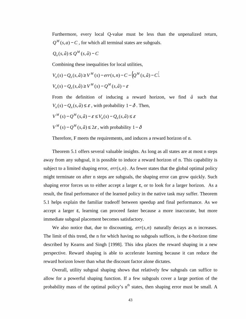
43
Furthermore, every local Q-value must be less than the unpenalized return,
CasQM −),( , for which all terminal states are subgoals.
CasQasQ Mn −≤ )ˆ,()ˆ,(
Combining these inequalities for local utilities,
( )CasQCnserrsVasQsV MMnn −−−−≥− )ˆ,(),()()ˆ,()(
ε−−≥− )ˆ,()()ˆ,()( asQsVasQsV MMnn
From the definition of inducing a reward horizon, we finda such that
ε≤− )ˆ,()( asQsV nn , with probability δ−1 . Then,
εε ≤−≤−− )ˆ,()()ˆ,()( asQsVasQsV nnMM
ε2)ˆ,()( ≤− asQsV MM , with probability δ−1
Therefore, F meets the requirements, and induces a reward horizon of n. �
Theorem 5.1 offers several valuable insights. As long as all states are at most n steps
away from any subgoal, it is possible to induce a reward horizon of n. This capability is
subject to a limited shaping error, ),( nserr . As fewer states that the global optimal policy
might terminate on after n steps are subgoals, the shaping error can grow quickly. Such
shaping error forces us to either accept a largerε, or to look for a larger horizon. As a
result, the final performance of the learned policy in the native task may suffer. Theorem
5.1 helps explain the familiar tradeoff between speedup and final performance. As we
accept a largerε, learning can proceed faster because a more inaccurate, but more
immediate subgoal placement becomes satisfactory.
We also notice that, due to discounting, ),( nserr naturally decays as n increases.
The limit of this trend, the n for which having no subgoals suffices, is theε-horizon time
described by Kearns and Singh [1998]. This idea places the reward shaping in a new
perspective. Reward shaping is able to accelerate learning because it can reduce the
reward horizon lower than what the discount factor alone dictates.
Overall, utility subgoal shaping shows that relatively few subgoals can suffice to
allow for a powerful shaping function. If a few subgoals cover a large portion of the
probability mass of the optimal policy’s nth states, then shaping error must be small. A
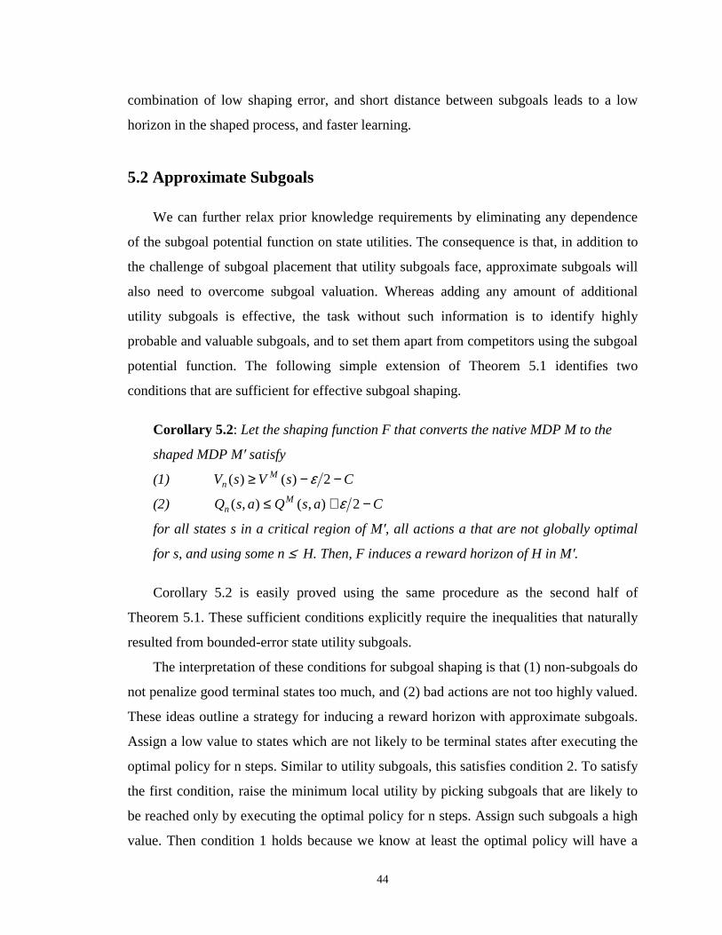
44
combination of low shaping error, and short distance between subgoals leads to a low
horizon in the shaped process, and faster learning.
5.2 Approximate Subgoals
We can further relax prior knowledge requirements by eliminating any dependence
of the subgoal potential function on state utilities. The consequence is that, in addition to
the challenge of subgoal placement that utility subgoals face, approximate subgoals will
also need to overcome subgoal valuation. Whereas adding any amount of additional
utility subgoals is effective, the task without such information is to identify highly
probable and valuable subgoals, and to set them apart from competitors using the subgoal
potential function. The following simple extension of Theorem 5.1 identifies two
conditions that are sufficient for effective subgoal shaping.
Corollary 5.2: Let the shaping function F that converts the native MDP M to the
shaped MDP Mÿ satisfy
(1) CsVsV Mn −−≥ 2)()( ε
(2) CasQasQ Mn −+≤ 2),(),( ε
for all states s in a critical region of Mÿ, all actions a that are not globally optimal
for s, and using some n≤ H. Then, F induces a reward horizon of H in Mÿ.
Corollary 5.2 is easily proved using the same procedure as the second half of
Theorem 5.1. These sufficient conditions explicitly require the inequalities that naturally
resulted from bounded-error state utility subgoals.
The interpretation of these conditions for subgoal shaping is that (1) non-subgoals do
not penalize good terminal states too much, and (2) bad actions are not too highly valued.
These ideas outline a strategy for inducing a reward horizon with approximate subgoals.
Assign a low value to states which are not likely to be terminal states after executing the
optimal policy for n steps. Similar to utility subgoals, this satisfies condition 2. To satisfy
the first condition, raise the minimum local utility by picking subgoals that are likely to
be reached only by executing the optimal policy for n steps. Assign such subgoals a high
value. Then condition 1 holds because we know at least the optimal policy will have a
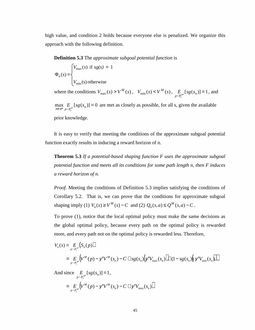
45
high value, and condition 2 holds because everyone else is penalized. We organize this
approach with the following definition.
Definition 5.3 Theapproximate subgoal potential functionis
otherwise(s)
)(
1if)(
min
max
V
s
sg(s)sV
a =Φ=
where the conditions )()(max sVsV M> , )()(min sVsV M< , 1)]([*~
=nPp
ssgEsπ
, and
0)]([max~*
=≠ n
PpssgE
sπππ
are met as closely as possible, for all s, given the available
prior knowledge.
It is easy to verify that meeting the conditions of the approximate subgoal potential
function exactly results in inducing a reward horizon of n.
Theorem 5.3If a potential-based shaping function F uses the approximate subgoal
potential function and meets all its conditions for some path length n, then F induces
a reward horizon of n.
Proof. Meeting the conditions of Definition 5.3 implies satisfying the conditions of
Corollary 5.2. That is, we can prove that the conditions for approximate subgoal
shaping imply (1) CsVsV Mn −≥ )()( and (2) CasQasQ M
n −≤ ),(),( .
To prove (1), notice that the local optimal policy must make the same decisions as
the global optimal policy, because every path on the optimal policy is rewarded
more, and every path not on the optimal policy is rewarded less. Therefore,
( ))()(*~
pSEsV nPp
nsπ
=
( ) ( )( ))())(1()()()()( minmax~ * n
nnn
nnn
MnM
PpsVssgsVssgCsVpVE
s
γγγπ
−++−−=
And since 1)]([*~
=nPp
ssgEsπ
,
( ))()()( max~ * n
nn
MnM
PpsVCsVpVE
s
γγπ
+−−=

46
( ))()()( max~ * n
Mnn
n
Pp
M sVsVECsVs
γγπ
−+−=
And with )()(max sVsV M> for all s, CsVsV Mn −> )()( .
Similarly, we can prove (2). Letπ be a non-optimal policy that executes action a
first, and executes optimal actions thereafter.
( ))(),(~
pSEasQ nPp
nsπ
=
( ) ( )( ))())(1()()()()( minmax~
nn
nnn
nnMnM
PpsVssgsVssgCsVpVE
s
γγγπ
−++−−=
And since 0)]([max~*
=≠ n
PpssgE
sπππ
,
( ))()()( min~
nn
nMnM
PpsVCsVpVE
s
γγπ
+−−=
( ))()(),( min~ * n
Mnn
n
Pp
M sVsVECasQs
γγπ
−+−=
And with )()(min sVsV M< for all s, CasQasQ Mn −< ),(),( . �
It is important to realize that the requirements of the approximate subgoal potential
function definition can be broken. For example, giving out too much penalty with
)(min sV or leaving out optimal terminal states can be partially corrected with larger
)(max sV values. The extent to which the requirements are violated dictates the
approximation of the shaping function. A larger approximation means more shaping
error. And just as before, more shaping error requires either accepting a largerε, or
looking farther for a reward horizon.

47
CHAPTER6
Dynamic Shaping
Shaping with approximate subgoals is one method to incorporate incomplete and
imperfect prior knowledge into the learning process. But it still requires the ability to
translate knowledge into rewards that a reinforcement learning agent can appreciate and
understand. When such a translation is apparent, the standard method of transforming the
native Markov decision process to a shaped one before learning is a successful technique.
In other cases, the precise choice of subgoals and how to value them may not be well
defined or easy to specify given the prior knowledge. Under these circumstances,
dynamic shaping is available to automatically translate the intended behaviors, in the
language of the prior knowledge, to specific rewards, in the language of reinforcement
learning algorithms.
Prior knowledge is often available in the form of high level concepts that are
ambiguous when interpreted at the low level of rewarding individual decisions. Perhaps
the knowledge is disjunctive, so that a number of mutually exclusive reward functions are
consistent with our prior beliefs. Perhaps it is qualitative. Then our knowledge is
consistent with any element of a parameterized family of reward functions. These types
of knowledge determine a space of possibilities for rewarding a task, but often the best
element is not apparent in advance. Finding the best element can be handled with a new
learning problem – to learn the best shaping function given the prior knowledge and some
experience of the task. This embedded learning problem is dynamic shaping.
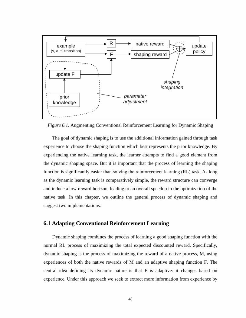
48
Figure 6.1. Augmenting Conventional Reinforcement Learning for Dynamic Shaping
The goal of dynamic shaping is to use the additional information gained through task
experience to choose the shaping function which best represents the prior knowledge. By
experiencing the native learning task, the learner attempts to find a good element from
the dynamic shaping space. But it is important that the process of learning the shaping
function is significantly easier than solving the reinforcement learning (RL) task. As long
as the dynamic learning task is comparatively simple, the reward structure can converge
and induce a low reward horizon, leading to an overall speedup in the optimization of the
native task. In this chapter, we outline the general process of dynamic shaping and
suggest two implementations.
6.1 Adapting Conventional Reinforcement Learning
Dynamic shaping combines the process of learning a good shaping function with the
normal RL process of maximizing the total expected discounted reward. Specifically,
dynamic shaping is the process of maximizing the reward of a native process, M, using
experiences of both the native rewards of M and an adaptive shaping function F. The
central idea defining its dynamic nature is that F is adaptive: it changes based on
experience. Under this approach we seek to extract more information from experience by
example(s, a, s’ transition)
R
F
native reward
shaping reward
updatepolicy
update F
priorknowledge
parameteradjustment
shapingintegration
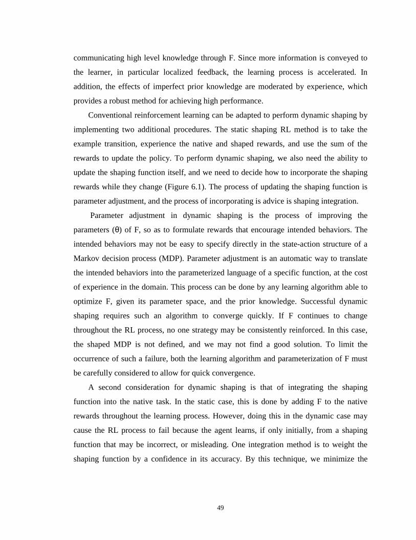
49
communicating high level knowledge through F. Since more information is conveyed to
the learner, in particular localized feedback, the learning process is accelerated. In
addition, the effects of imperfect prior knowledge are moderated by experience, which
provides a robust method for achieving high performance.
Conventional reinforcement learning can be adapted to perform dynamic shaping by
implementing two additional procedures. The static shaping RL method is to take the
example transition, experience the native and shaped rewards, and use the sum of the
rewards to update the policy. To perform dynamic shaping, we also need the ability to
update the shaping function itself, and we need to decide how to incorporate the shaping
rewards while they change (Figure 6.1). The process of updating the shaping function is
parameter adjustment, and the process of incorporating is advice is shaping integration.
Parameter adjustment in dynamic shaping is the process of improving the
parameters (θ) of F, so as to formulate rewards that encourage intended behaviors. The
intended behaviors may not be easy to specify directly in the state-action structure of a
Markov decision process (MDP). Parameter adjustment is an automatic way to translate
the intended behaviors into the parameterized language of a specific function, at the cost
of experience in the domain. This process can be done by any learning algorithm able to
optimize F, given its parameter space, and the prior knowledge. Successful dynamic
shaping requires such an algorithm to converge quickly. If F continues to change
throughout the RL process, no one strategy may be consistently reinforced. In this case,
the shaped MDP is not defined, and we may not find a good solution. To limit the
occurrence of such a failure, both the learning algorithm and parameterization of F must
be carefully considered to allow for quick convergence.
A second consideration for dynamic shaping is that of integrating the shaping
function into the native task. In the static case, this is done by adding F to the native
rewards throughout the learning process. However, doing this in the dynamic case may
cause the RL process to fail because the agent learns, if only initially, from a shaping
function that may be incorrect, or misleading. One integration method is to weight the
shaping function by a confidence in its accuracy. By this technique, we minimize the
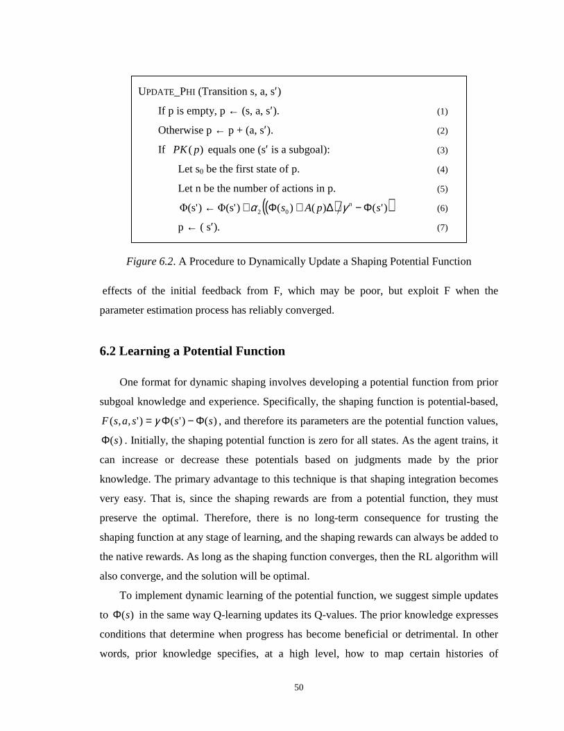
50
Figure 6.2. A Procedure to Dynamically Update a Shaping Potential Function
effects of the initial feedback from F, which may be poor, but exploit F when the
parameter estimation process has reliably converged.
6.2 Learning a Potential Function
One format for dynamic shaping involves developing a potential function from prior
subgoal knowledge and experience. Specifically, the shaping function is potential-based,
)()'()',,( sssasF Φ−Φ= γ , and therefore its parameters are the potential function values,
)(sΦ . Initially, the shaping potential function is zero for all states. As the agent trains, it
can increase or decrease these potentials based on judgments made by the prior
knowledge. The primary advantage to this technique is that shaping integration becomes
very easy. That is, since the shaping rewards are from a potential function, they must
preserve the optimal. Therefore, there is no long-term consequence for trusting the
shaping function at any stage of learning, and the shaping rewards can always be added to
the native rewards. As long as the shaping function converges, then the RL algorithm will
also converge, and the solution will be optimal.
To implement dynamic learning of the potential function, we suggest simple updates
to )(sΦ in the same way Q-learning updates its Q-values. The prior knowledge expresses
conditions that determine when progress has become beneficial or detrimental. In other
words, prior knowledge specifies, at a high level, how to map certain histories of
UPDATE_PHI (Transition s, a, s′)
If p is empty, p← (s, a, s′). (1)
Otherwise p← p + (a, s′). (2)
If )( pPK equals one (s′ is a subgoal): (3)
Let s0 be the first state of p. (4)
Let n be the number of actions in p. (5)
( )( ))'()()()� (s')� (s' 02 spAs n Φ−∆+Φ+← γα (6)
p ← ( s′). (7)
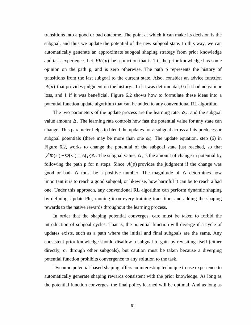
51
transitions into a good or bad outcome. The point at which it can make its decision is the
subgoal, and thus we update the potential of the new subgoal state. In this way, we can
automatically generate an approximate subgoal shaping strategy from prior knowledge
and task experience. Let )( pPK be a function that is 1 if the prior knowledge has some
opinion on the path p, and is zero otherwise. The path p represents the history of
transitions from the last subgoal to the current state. Also, consider an advice function
)( pA that provides judgment on the history: -1 if it was detrimental, 0 if it had no gain or
loss, and 1 if it was beneficial. Figure 6.2 shows how to formulate these ideas into a
potential function update algorithm that can be added to any conventional RL algorithm.
The two parameters of the update process are the learning rate,2α , and the subgoal
value amount∆ . The learning rate controls how fast the potential value for any state can
change. This parameter helps to blend the updates for a subgoal across all its predecessor
subgoal potentials (there may be more than one s0). The update equation, step (6) in
Figure 6.2, works to change the potential of the subgoal state just reached, so that
∆=Φ−Φ )()()'( 0 pAssnγ . The subgoal value,∆ , is the amount of change in potential by
following the path p for n steps. Since )( pA provides the judgment if the change was
good or bad, ∆ must be a positive number. The magnitude of∆ determines how
important it is to reach a good subgoal, or likewise, how harmful it can be to reach a bad
one. Under this approach, any conventional RL algorithm can perform dynamic shaping
by defining Update-Phi, running it on every training transition, and adding the shaping
rewards to the native rewards throughout the learning process.
In order that the shaping potential converges, care must be taken to forbid the
introduction of subgoal cycles. That is, the potential function will diverge if a cycle of
updates exists, such as a path where the initial and final subgoals are the same. Any
consistent prior knowledge should disallow a subgoal to gain by revisiting itself (either
directly, or through other subgoals), but caution must be taken because a diverging
potential function prohibits convergence to any solution to the task.
Dynamic potential-based shaping offers an interesting technique to use experience to
automatically generate shaping rewards consistent with the prior knowledge. As long as
the potential function converges, the final policy learned will be optimal. And as long as
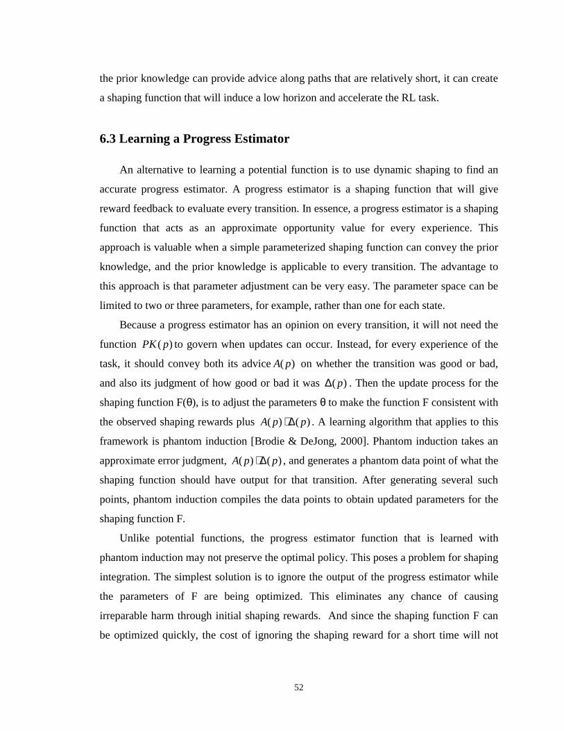
52
the prior knowledge can provide advice along paths that are relatively short, it can create
a shaping function that will induce a low horizon and accelerate the RL task.
6.3 Learning a Progress Estimator
An alternative to learning a potential function is to use dynamic shaping to find an
accurate progress estimator. A progress estimator is a shaping function that will give
reward feedback to evaluate every transition. In essence, a progress estimator is a shaping
function that acts as an approximate opportunity value for every experience. This
approach is valuable when a simple parameterized shaping function can convey the prior
knowledge, and the prior knowledge is applicable to every transition. The advantage to
this approach is that parameter adjustment can be very easy. The parameter space can be
limited to two or three parameters, for example, rather than one for each state.
Because a progress estimator has an opinion on every transition, it will not need the
function )( pPK to govern when updates can occur. Instead, for every experience of the
task, it should convey both its advice )( pA on whether the transition was good or bad,
and also its judgment of how good or bad it was )( p∆ . Then the update process for the
shaping function F(θ), is to adjust the parametersθ to make the function F consistent with
the observed shaping rewards plus )()( ppA ∆⋅ . A learning algorithm that applies to this
framework is phantom induction [Brodie & DeJong, 2000]. Phantom induction takes an
approximate error judgment, )()( ppA ∆⋅ , and generates a phantom data point of what the
shaping function should have output for that transition. After generating several such
points, phantom induction compiles the data points to obtain updated parameters for the
shaping function F.
Unlike potential functions, the progress estimator function that is learned with
phantom induction may not preserve the optimal policy. This poses a problem for shaping
integration. The simplest solution is to ignore the output of the progress estimator while
the parameters of F are being optimized. This eliminates any chance of causing
irreparable harm through initial shaping rewards. And since the shaping function F can
be optimized quickly, the cost of ignoring the shaping reward for a short time will not

53
delay convergence significantly. Once the shaping function converges to a good
parameter set, it can be added to native rewards just as in the static case.
Using phantom induction to learn the parameters of F will find the shaping function
most consistent with the prior knowledge. If the resulting progress estimator
approximates the opportunity value of each transition close enough, then the RL
algorithm can converge to a good policy quickly, since opportunity value induces a
reward horizon of one.
54
CHAPTER7
Stochastic Gridworld
A commonly used test application for reinforcement learning algorithms is the
gridworld domain. This problem involves a two dimensional grid state space in which the
learning agent can move in one of four cardinal directions through the extent of the grid.
The learning tasks in such domains are varied, with the most common being moving to
one goal state, moving through a sequence of goal states, navigating mazes, navigating
rooms, and making taxi fares. While simple to design, gridworld problems can be
challenging, and are useful to clearly observe the strengths and weaknesses of an
approach.
We apply reward shaping to a stochastic, goal-state gridworld problem. The
stochastic gridworld is used in other reward shaping work [Ng et al, 1999; Wiewiora et
al, 2003]. For this task, the learning agent must travel from the lower left corner of a
square grid, to the upper right corner in as few actions as possible. The actions are
stochastic, so that they move the agent in unintended directions randomly. We apply
reward shaping to this standard test domain to demonstrate our analytical results and
practical techniques for reward shaping: the reward horizon, opportunity value, subgoal
shaping, and dynamic shaping.
7.1 The Gridworld Task
The stochastic gridworld used in the experiments of this chapter requires a learner to
achieve a goal state with as few actions as possible, using non-deterministic actions. The
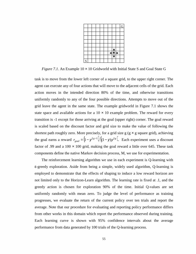
55
Figure 7.1. An Example 10× 10 Gridworld with Initial State S and Goal State G
task is to move from the lower left corner of a square grid, to the upper right corner. The
agent can execute any of four actions that will move to the adjacent cells of the grid. Each
action moves in the intended direction 80% of the time, and otherwise transitions
uniformly randomly to any of the four possible directions. Attempts to move out of the
grid leave the agent in the same state. The example gridworld in Figure 7.1 shows the
state space and available actions for a 10× 10 example problem. The reward for every
transition is -1 except for those arriving at the goal (upper right) corner. The goal reward
is scaled based on the discount factor and grid size to make the value of following the
shortest path roughly zero. More precisely, for a grid size g (g× g square grid), achieving
the goal earns a reward ( ) ( )gggoalr 212 )1(1 γγγ −−= − . Each experiment uses a discount
factor of .99 and a 100× 100 grid, making the goal reward a little over 645. These task
components define the native Markov decision process, M, we use for experimentation.
The reinforcement learning algorithm we use in each experiment is Q-learning with
ε-greedy exploration. Aside from being a simple, widely used algorithm, Q-learning is
employed to demonstrate that the effects of shaping to induce a low reward horizon are
not limited only to the Horizon-Learn algorithm. The learning rate is fixed at .1, and the
greedy action is chosen for exploration 90% of the time. Initial Q-values are set
uniformly randomly with mean zero. To judge the level of performance as training
progresses, we evaluate the return of the current policy over ten trials and report the
average. Note that our procedure for evaluating and reporting policy performance differs
from other works in this domain which report the performance observed during training.
Each learning curve is shown with 95% confidence intervals about the average
performance from data generated by 100 trials of the Q-learning process.
•
G
S
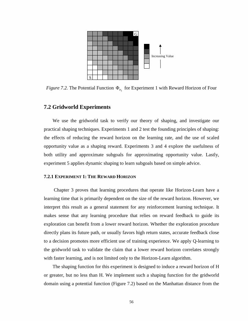
56
Figure 7.2.The Potential Function1e� for Experiment 1 with Reward Horizon of Four
7.2 Gridworld Experiments
We use the gridworld task to verify our theory of shaping, and investigate our
practical shaping techniques. Experiments 1 and 2 test the founding principles of shaping:
the effects of reducing the reward horizon on the learning rate, and the use of scaled
opportunity value as a shaping reward. Experiments 3 and 4 explore the usefulness of
both utility and approximate subgoals for approximating opportunity value. Lastly,
experiment 5 applies dynamic shaping to learn subgoals based on simple advice.
7.2.1 EXPERIMENT 1: THE REWARD HORIZON
Chapter 3 proves that learning procedures that operate like Horizon-Learn have a
learning time that is primarily dependent on the size of the reward horizon. However, we
interpret this result as a general statement for any reinforcement learning technique. It
makes sense that any learning procedure that relies on reward feedback to guide its
exploration can benefit from a lower reward horizon. Whether the exploration procedure
directly plans its future path, or usually favors high return states, accurate feedback close
to a decision promotes more efficient use of training experience. We apply Q-learning to
the gridworld task to validate the claim that a lower reward horizon correlates strongly
with faster learning, and is not limited only to the Horizon-Learn algorithm.
The shaping function for this experiment is designed to induce a reward horizon of H
or greater, but no less than H. We implement such a shaping function for the gridworld
domain using a potential function (Figure 7.2) based on the Manhattan distance from the
G
S
Increasing Value
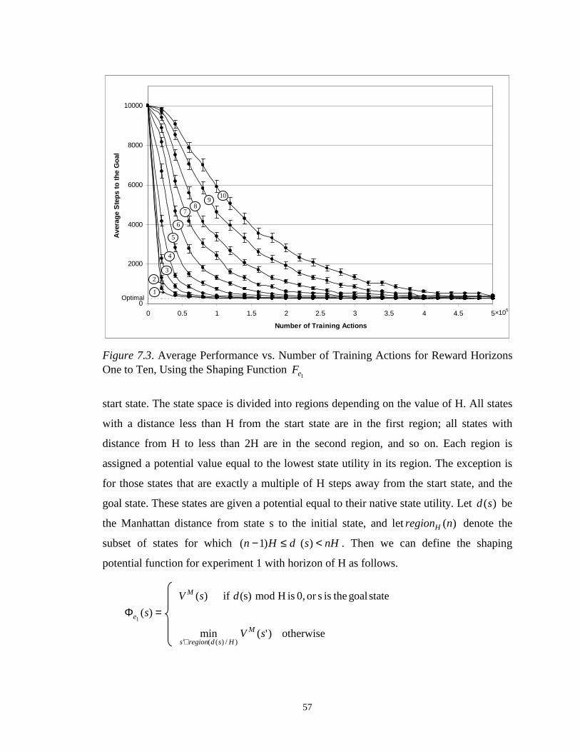
57
Figure 7.3. Average Performance vs. Number of Training Actions for Reward HorizonsOne to Ten, Using the Shaping Function
1eF
start state. The state space is divided into regions depending on the value of H. All states
with a distance less than H from the start state are in the first region; all states with
distance from H to less than 2H are in the second region, and so on. Each region is
assigned a potential value equal to the lowest state utility in its region. The exception is
for those states that are exactly a multiple of H steps away from the start state, and the
goal state. These states are given a potential equal to their native state utility. Let)(sd be
the Manhattan distance from state s to the initial state, and let )(nregionH denote the
subset of states for which nHsdHn <≤− )()1( . Then we can define the shaping
potential function for experiment 1 with horizon of H as follows.
otherwise)'(min
)(
stategoaltheissor0,isHmod(s)if)(
)/)(('
1
sV
s
dsV
M
Hsdregions
e
M
∈
=Φ
0
2000
4000
6000
8000
10000
0 0.5 1 1.5 2 2.5 3 3.5 4 4.5 5
Number of Training Actions
Ave
rage
Ste
psto
the
Goa
l
×105
Optimal
109
7
6
5
4
32
1
8
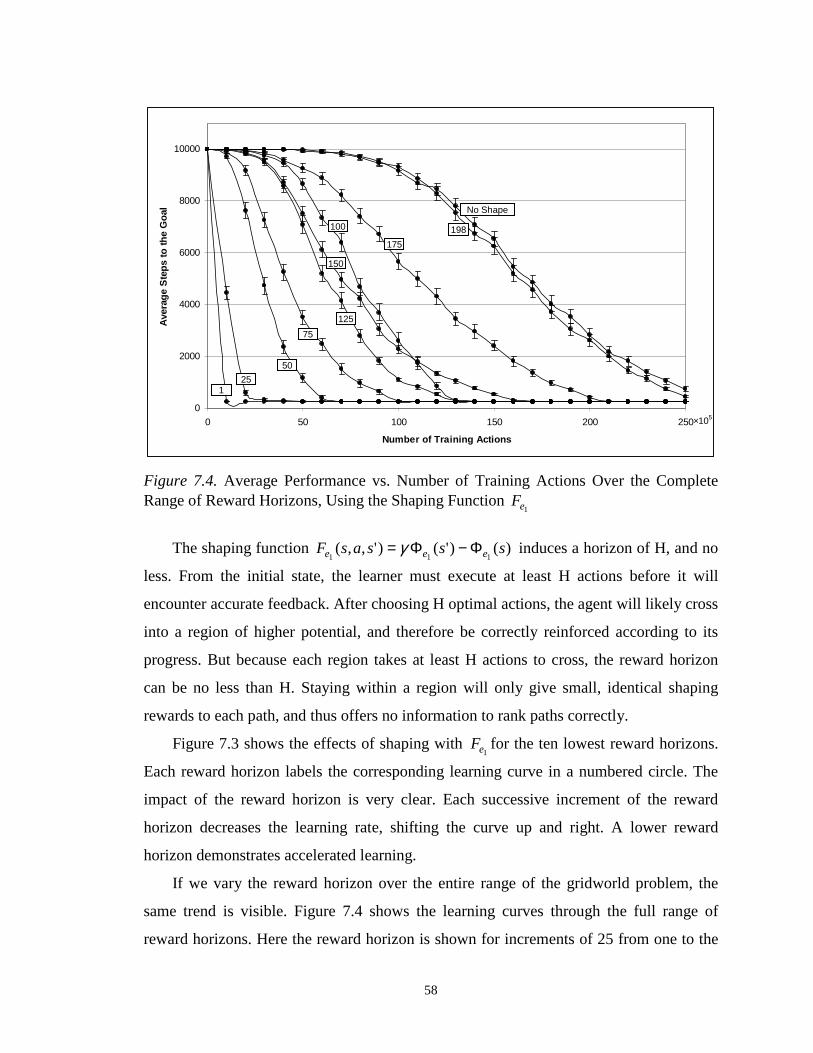
58
Figure 7.4.Average Performance vs. Number of Training Actions Over the CompleteRange of Reward Horizons, Using the Shaping Function
1eF
The shaping function )()'()',,(111
sssasF eee Φ−Φ= γ induces a horizon of H, and no
less. From the initial state, the learner must execute at least H actions before it will
encounter accurate feedback. After choosing H optimal actions, the agent will likely cross
into a region of higher potential, and therefore be correctly reinforced according to its
progress. But because each region takes at least H actions to cross, the reward horizon
can be no less than H. Staying within a region will only give small, identical shaping
rewards to each path, and thus offers no information to rank paths correctly.
Figure 7.3 shows the effects of shaping with1e
F for the ten lowest reward horizons.
Each reward horizon labels the corresponding learning curve in a numbered circle. The
impact of the reward horizon is very clear. Each successive increment of the reward
horizon decreases the learning rate, shifting the curve up and right. A lower reward
horizon demonstrates accelerated learning.
If we vary the reward horizon over the entire range of the gridworld problem, the
same trend is visible. Figure 7.4 shows the learning curves through the full range of
reward horizons. Here the reward horizon is shown for increments of 25 from one to the
0
2000
4000
6000
8000
10000
0 50 100 150 200 250
Number of Training Actions
Ave
rage
Ste
psto
the
Goa
l
×105
198
No Shape
175
150
125
100
75
50
251
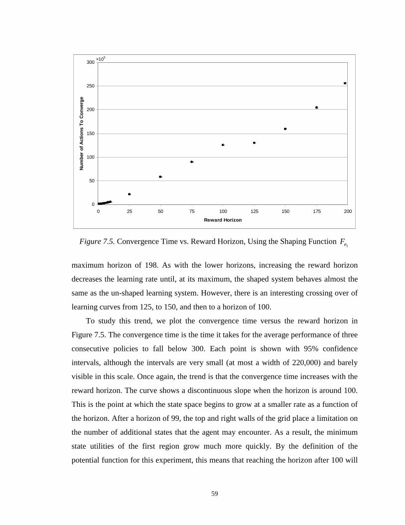
59
Figure 7.5.Convergence Time vs. Reward Horizon, Using the Shaping Function1e
F
maximum horizon of 198. As with the lower horizons, increasing the reward horizon
decreases the learning rate until, at its maximum, the shaped system behaves almost the
same as the un-shaped learning system. However, there is an interesting crossing over of
learning curves from 125, to 150, and then to a horizon of 100.
To study this trend, we plot the convergence time versus the reward horizon in
Figure 7.5. The convergence time is the time it takes for the average performance of three
consecutive policies to fall below 300. Each point is shown with 95% confidence
intervals, although the intervals are very small (at most a width of 220,000) and barely
visible in this scale. Once again, the trend is that the convergence time increases with the
reward horizon. The curve shows a discontinuous slope when the horizon is around 100.
This is the point at which the state space begins to grow at a smaller rate as a function of
the horizon. After a horizon of 99, the top and right walls of the grid place a limitation on
the number of additional states that the agent may encounter. As a result, the minimum
state utilities of the first region grow much more quickly. By the definition of the
potential function for this experiment, this means that reaching the horizon after 100 will
0
50
100
150
200
250
300
0 25 50 75 100 125 150 175 200
Reward Horizon
Num
ber
ofA
ctio
nsT
oC
onve
rge
×105
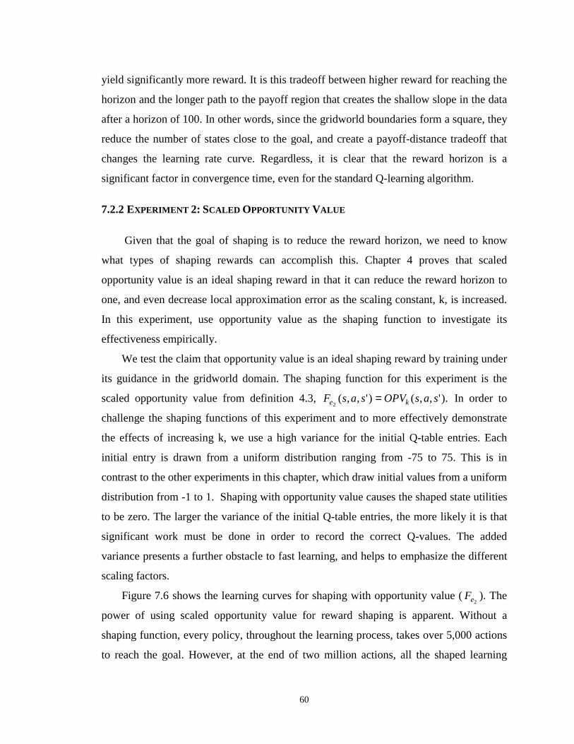
60
yield significantly more reward. It is this tradeoff between higher reward for reaching the
horizon and the longer path to the payoff region that creates the shallow slope in the data
after a horizon of 100. In other words, since the gridworld boundaries form a square, they
reduce the number of states close to the goal, and create a payoff-distance tradeoff that
changes the learning rate curve. Regardless, it is clear that the reward horizon is a
significant factor in convergence time, even for the standard Q-learning algorithm.
7.2.2 EXPERIMENT 2: SCALED OPPORTUNITY VALUE
Given that the goal of shaping is to reduce the reward horizon, we need to know
what types of shaping rewards can accomplish this. Chapter 4 proves that scaled
opportunity value is an ideal shaping reward in that it can reduce the reward horizon to
one, and even decrease local approximation error as the scaling constant, k, is increased.
In this experiment, use opportunity value as the shaping function to investigate its
effectiveness empirically.
We test the claim that opportunity value is an ideal shaping reward by training under
its guidance in the gridworld domain. The shaping function for this experiment is the
scaled opportunity value from definition 4.3, ).',,()',,(2
sasOPVsasF ke = In order to
challenge the shaping functions of this experiment and to more effectively demonstrate
the effects of increasing k, we use a high variance for the initial Q-table entries. Each
initial entry is drawn from a uniform distribution ranging from -75 to 75. This is in
contrast to the other experiments in this chapter, which draw initial values from a uniform
distribution from -1 to 1. Shaping with opportunity value causes the shaped state utilities
to be zero. The larger the variance of the initial Q-table entries, the more likely it is that
significant work must be done in order to record the correct Q-values. The added
variance presents a further obstacle to fast learning, and helps to emphasize the different
scaling factors.
Figure 7.6 shows the learning curves for shaping with opportunity value (2eF ). The
power of using scaled opportunity value for reward shaping is apparent. Without a
shaping function, every policy, throughout the learning process, takes over 5,000 actions
to reach the goal. However, at the end of two million actions, all the shaped learning
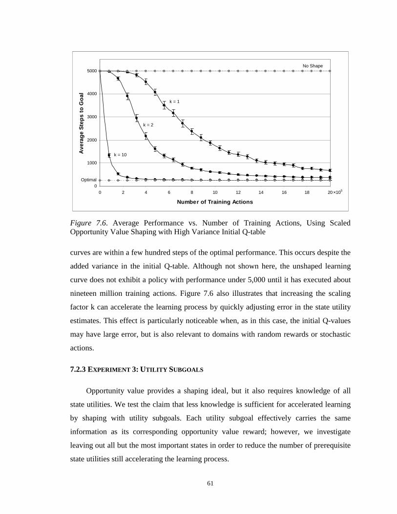
61
Figure 7.6. Average Performance vs. Number of Training Actions, Using ScaledOpportunity Value Shaping with High Variance Initial Q-table
curves are within a few hundred steps of the optimal performance. This occurs despite the
added variance in the initial Q-table. Although not shown here, the unshaped learning
curve does not exhibit a policy with performance under 5,000 until it has executed about
nineteen million training actions. Figure 7.6 also illustrates that increasing the scaling
factor k can accelerate the learning process by quickly adjusting error in the state utility
estimates. This effect is particularly noticeable when, as in this case, the initial Q-values
may have large error, but is also relevant to domains with random rewards or stochastic
actions.
7.2.3 EXPERIMENT 3: UTILITY SUBGOALS
Opportunity value provides a shaping ideal, but it also requires knowledge of all
state utilities. We test the claim that less knowledge is sufficient for accelerated learning
by shaping with utility subgoals. Each utility subgoal effectively carries the same
information as its corresponding opportunity value reward; however, we investigate
leaving out all but the most important states in order to reduce the number of prerequisite
state utilities still accelerating the learning process.
0
1000
2000
3000
4000
5000
0 2 4 6 8 10 12 14 16 18 20
Number of Training Actions
Ave
rage
Ste
psto
Goa
l
×105
Optimal
k = 10
k = 2
k = 1
No Shape
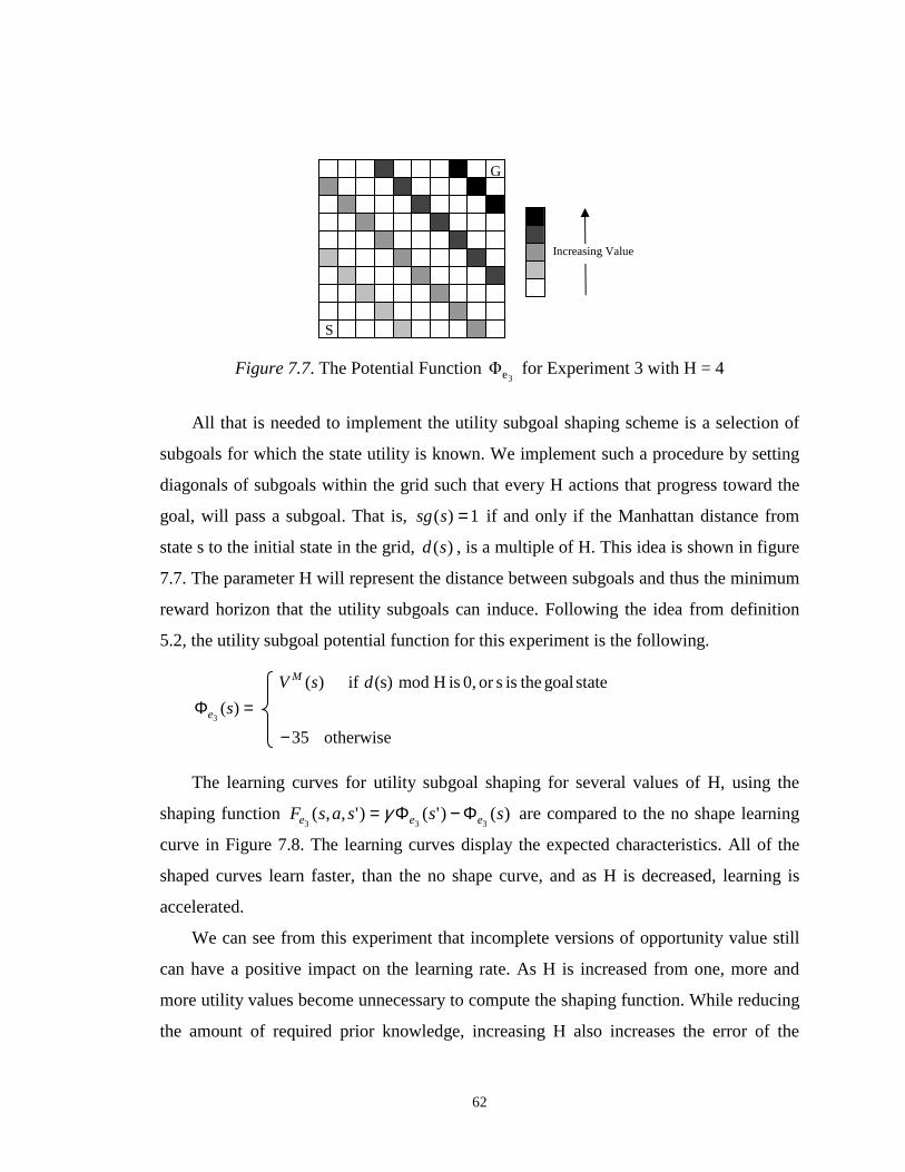
62
Figure 7.7. The Potential Function3e� for Experiment 3 with H = 4
All that is needed to implement the utility subgoal shaping scheme is a selection of
subgoals for which the state utility is known. We implement such a procedure by setting
diagonals of subgoals within the grid such that every H actions that progress toward the
goal, will pass a subgoal. That is, 1)( =ssg if and only if the Manhattan distance from
state s to the initial state in the grid, )(sd , is a multiple of H. This idea is shown in figure
7.7. The parameter H will represent the distance between subgoals and thus the minimum
reward horizon that the utility subgoals can induce. Following the idea from definition
5.2, the utility subgoal potential function for this experiment is the following.
otherwise35
)(
stategoaltheissor0,isHmod(s)if)(
3
−
=Φ s
dsV
e
M
The learning curves for utility subgoal shaping for several values of H, using the
shaping function )()'()',,(333
sssasF eee Φ−Φ= γ are compared to the no shape learning
curve in Figure 7.8. The learning curves display the expected characteristics. All of the
shaped curves learn faster, than the no shape curve, and as H is decreased, learning is
accelerated.
We can see from this experiment that incomplete versions of opportunity value still
can have a positive impact on the learning rate. As H is increased from one, more and
more utility values become unnecessary to compute the shaping function. While reducing
the amount of required prior knowledge, increasing H also increases the error of the
G
S
Increasing Value
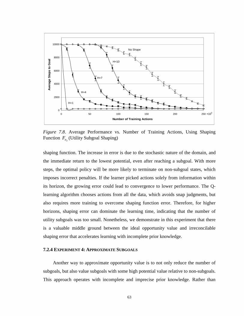
63
Figure 7.8. Average Performance vs. Number of Training Actions, Using ShapingFunction
3eF (Utility Subgoal Shaping)
shaping function. The increase in error is due to the stochastic nature of the domain, and
the immediate return to the lowest potential, even after reaching a subgoal. With more
steps, the optimal policy will be more likely to terminate on non-subgoal states, which
imposes incorrect penalties. If the learner picked actions solely from information within
its horizon, the growing error could lead to convergence to lower performance. The Q-
learning algorithm chooses actions from all the data, which avoids snap judgments, but
also requires more training to overcome shaping function error. Therefore, for higher
horizons, shaping error can dominate the learning time, indicating that the number of
utility subgoals was too small. Nonetheless, we demonstrate in this experiment that there
is a valuable middle ground between the ideal opportunity value and irreconcilable
shaping error that accelerates learning with incomplete prior knowledge.
7.2.4 EXPERIMENT 4: APPROXIMATE SUBGOALS
Another way to approximate opportunity value is to not only reduce the number of
subgoals, but also value subgoals with some high potential value relative to non-subgoals.
This approach operates with incomplete and imprecise prior knowledge. Rather than
Optimal0
2000
4000
6000
8000
10000
0 50 100 150 200 250
Number of Training Actions
Ave
rage
Ste
psto
Goa
l
×105
H=1
H=4
H=7
H=10
No Shape
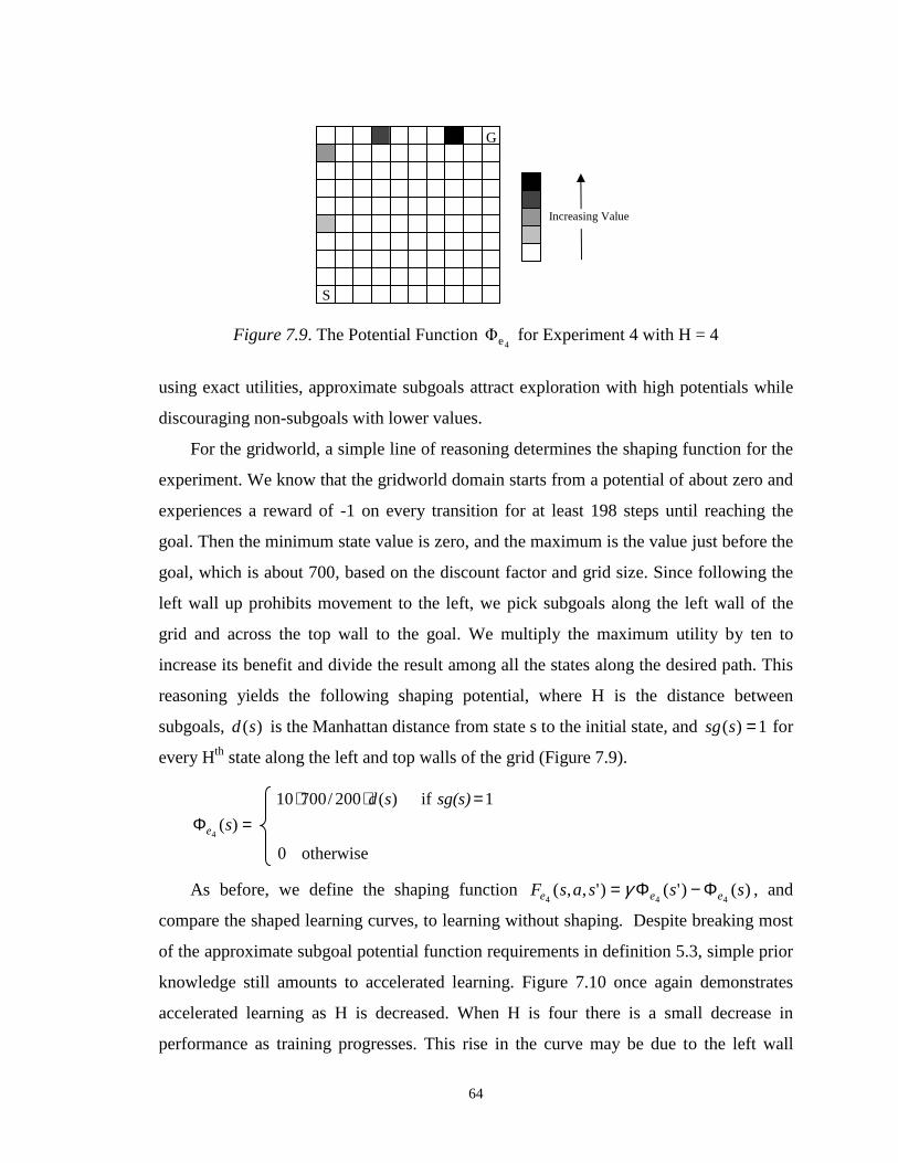
64
Figure 7.9. The Potential Function4e� for Experiment 4 with H = 4
using exact utilities, approximate subgoals attract exploration with high potentials while
discouraging non-subgoals with lower values.
For the gridworld, a simple line of reasoning determines the shaping function for the
experiment. We know that the gridworld domain starts from a potential of about zero and
experiences a reward of -1 on every transition for at least 198 steps until reaching the
goal. Then the minimum state value is zero, and the maximum is the value just before the
goal, which is about 700, based on the discount factor and grid size. Since following the
left wall up prohibits movement to the left, we pick subgoals along the left wall of the
grid and across the top wall to the goal. We multiply the maximum utility by ten to
increase its benefit and divide the result among all the states along the desired path. This
reasoning yields the following shaping potential, where H is the distance between
subgoals, )(sd is the Manhattan distance from state s to the initial state, and 1)( =ssg for
every Hth state along the left and top walls of the grid (Figure 7.9).
otherwise0
)(
1if)(200/70010
4=Φ
=⋅⋅s
sg(s)sd
e
As before, we define the shaping function )()'()',,(444
sssasF eee Φ−Φ= γ , and
compare the shaped learning curves, to learning without shaping. Despite breaking most
of the approximate subgoal potential function requirements in definition 5.3, simple prior
knowledge still amounts to accelerated learning. Figure 7.10 once again demonstrates
accelerated learning as H is decreased. When H is four there is a small decrease in
performance as training progresses. This rise in the curve may be due to the left wall
G
S
Increasing Value
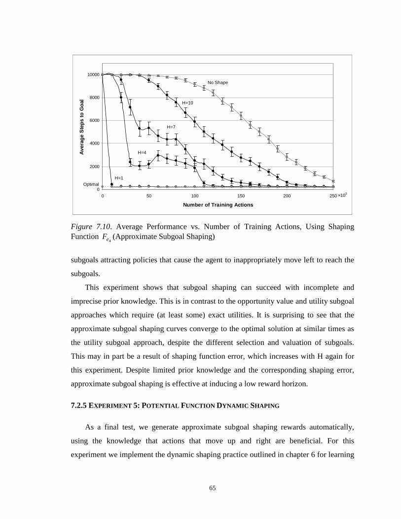
65
Figure 7.10. Average Performance vs. Number of Training Actions, Using ShapingFunction
4eF (Approximate Subgoal Shaping)
subgoals attracting policies that cause the agent to inappropriately move left to reach the
subgoals.
This experiment shows that subgoal shaping can succeed with incomplete and
imprecise prior knowledge. This is in contrast to the opportunity value and utility subgoal
approaches which require (at least some) exact utilities. It is surprising to see that the
approximate subgoal shaping curves converge to the optimal solution at similar times as
the utility subgoal approach, despite the different selection and valuation of subgoals.
This may in part be a result of shaping function error, which increases with H again for
this experiment. Despite limited prior knowledge and the corresponding shaping error,
approximate subgoal shaping is effective at inducing a low reward horizon.
7.2.5 EXPERIMENT 5: POTENTIAL FUNCTION DYNAMIC SHAPING
As a final test, we generate approximate subgoal shaping rewards automatically,
using the knowledge that actions that move up and right are beneficial. For this
experiment we implement the dynamic shaping practice outlined in chapter 6 for learning
0
2000
4000
6000
8000
10000
0 50 100 150 200 250
Number of Training Actions
Ave
rage
Ste
psto
Goa
l
×105
H=1
H=4
H=7
H=10
No Shape
Optimal
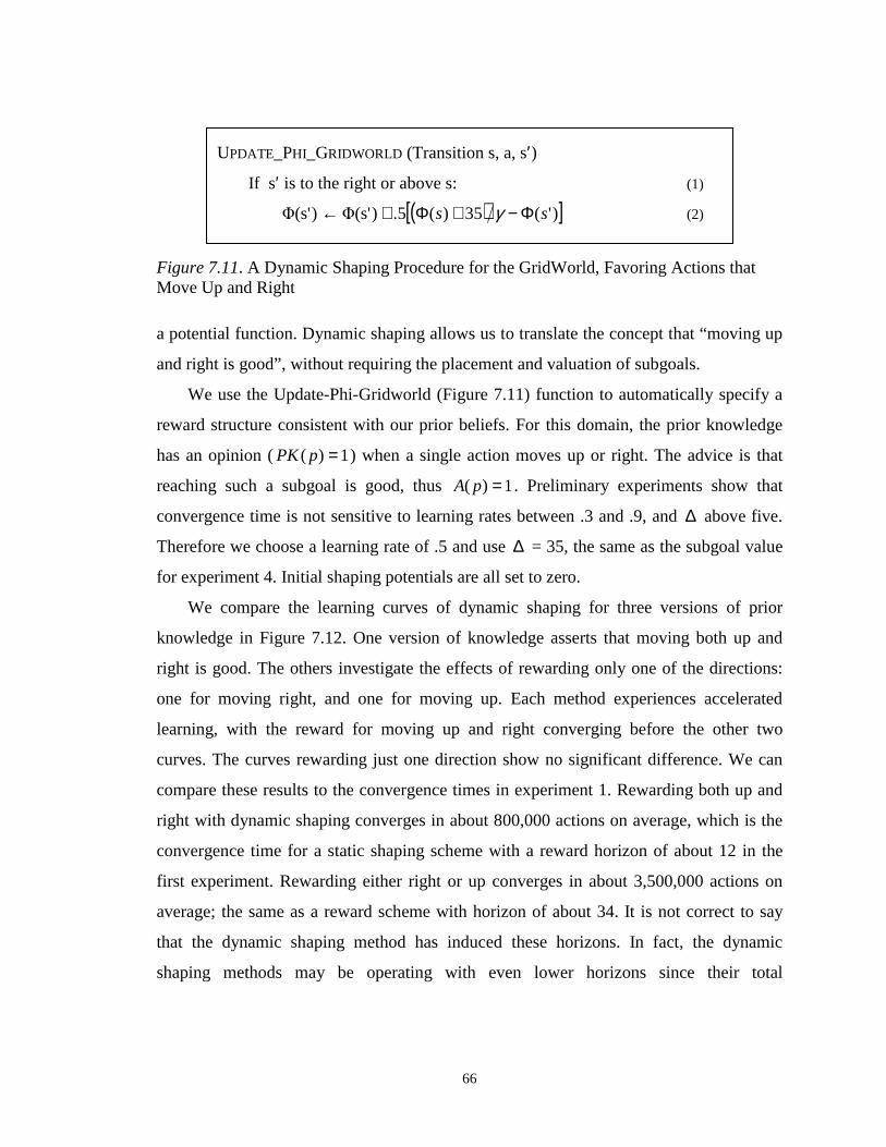
66
Figure 7.11. A Dynamic Shaping Procedure for the GridWorld, Favoring Actions thatMove Up and Right
a potential function. Dynamic shaping allows us to translate the concept that “moving up
and right is good”, without requiring the placement and valuation of subgoals.
We use the Update-Phi-Gridworld (Figure 7.11) function to automatically specify a
reward structure consistent with our prior beliefs. For this domain, the prior knowledge
has an opinion ( 1)( =pPK ) when a single action moves up or right. The advice is that
reaching such a subgoal is good, thus 1)( =pA . Preliminary experiments show that
convergence time is not sensitive to learning rates between .3 and .9, and∆ above five.
Therefore we choose a learning rate of .5 and use∆ = 35, the same as the subgoal value
for experiment 4. Initial shaping potentials are all set to zero.
We compare the learning curves of dynamic shaping for three versions of prior
knowledge in Figure 7.12. One version of knowledge asserts that moving both up and
right is good. The others investigate the effects of rewarding only one of the directions:
one for moving right, and one for moving up. Each method experiences accelerated
learning, with the reward for moving up and right converging before the other two
curves. The curves rewarding just one direction show no significant difference. We can
compare these results to the convergence times in experiment 1. Rewarding both up and
right with dynamic shaping converges in about 800,000 actions on average, which is the
convergence time for a static shaping scheme with a reward horizon of about 12 in the
first experiment. Rewarding either right or up converges in about 3,500,000 actions on
average; the same as a reward scheme with horizon of about 34. It is not correct to say
that the dynamic shaping method has induced these horizons. In fact, the dynamic
shaping methods may be operating with even lower horizons since their total
UPDATE_PHI_GRIDWORLD (Transition s, a, s′)
If s′ is to the right or above s: (1)
( )[ ])'(35)(5.)� (s')� (s' ss Φ−+Φ+← γ (2)
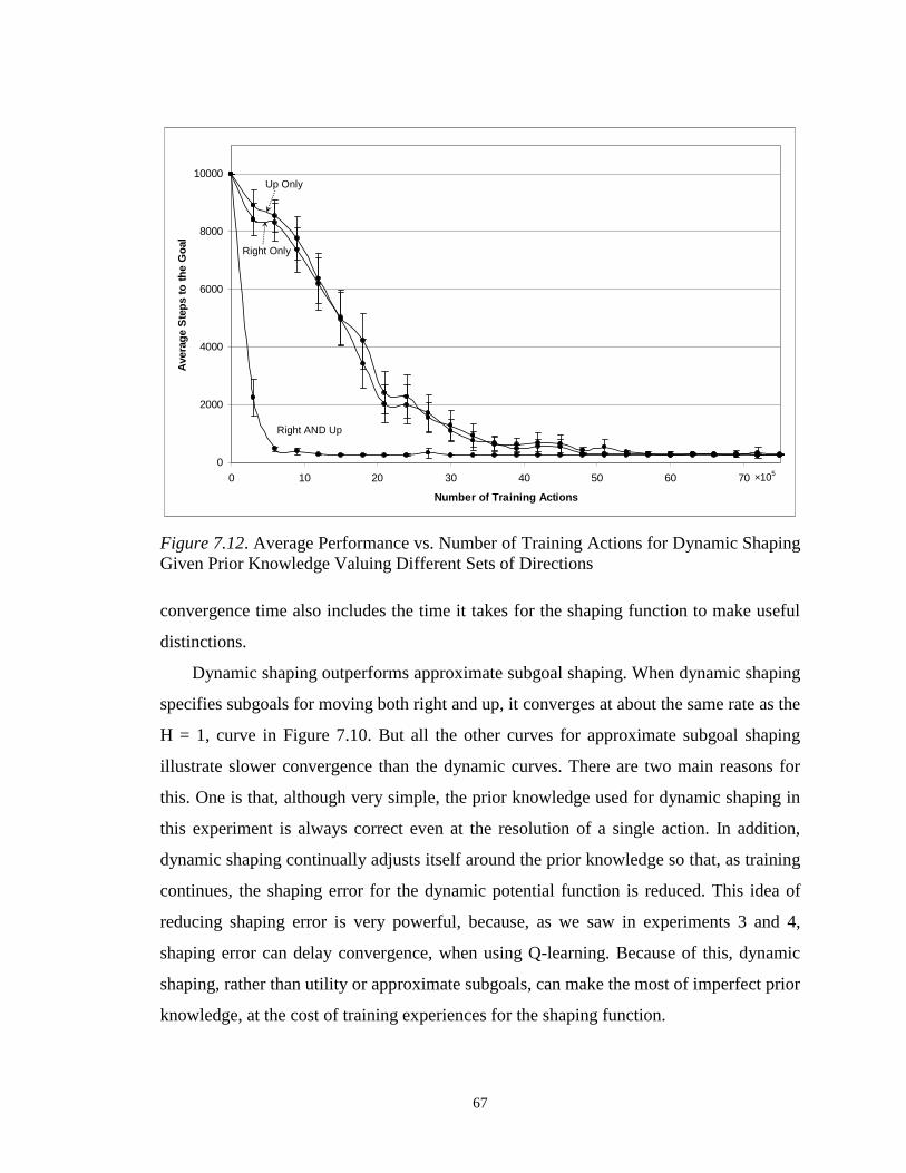
67
Figure 7.12. Average Performance vs. Number of Training Actions for Dynamic ShapingGiven Prior Knowledge Valuing Different Sets of Directions
convergence time also includes the time it takes for the shaping function to make useful
distinctions.
Dynamic shaping outperforms approximate subgoal shaping. When dynamic shaping
specifies subgoals for moving both right and up, it converges at about the same rate as the
H = 1, curve in Figure 7.10. But all the other curves for approximate subgoal shaping
illustrate slower convergence than the dynamic curves. There are two main reasons for
this. One is that, although very simple, the prior knowledge used for dynamic shaping in
this experiment is always correct even at the resolution of a single action. In addition,
dynamic shaping continually adjusts itself around the prior knowledge so that, as training
continues, the shaping error for the dynamic potential function is reduced. This idea of
reducing shaping error is very powerful, because, as we saw in experiments 3 and 4,
shaping error can delay convergence, when using Q-learning. Because of this, dynamic
shaping, rather than utility or approximate subgoals, can make the most of imperfect prior
knowledge, at the cost of training experiences for the shaping function.
0
2000
4000
6000
8000
10000
0 10 20 30 40 50 60 70
Number of Training Actions
Ave
rage
Ste
psto
the
Goa
l
×105
Right AND Up
Up Only
Right Only
68
CHAPTER8
Bipedal Walking
Although useful to provide a clear demonstration of the principles of shaping, the
stochastic gridworld is an application limited by its simple and artificial nature. For
example, the gridworld has no interesting prior knowledge to apply beyond what we have
already investigated. In order to provide a more complex problem that can use real world
domain knowledge, we investigate the reward shaping process in a bipedal walking task.
In this chapter, we apply reward shaping to bipedal walking with a round-footed
mechanism. The task is to walk as far as possible within a given amount of time, starting
from an upright, motionless position. The control inputs are torques for rocking and leg
swinging. These torques cause rotational accelerations that are configuration dependent,
and thereby interact in nonlinear ways. Control torques are too weak to force the
mechanism to follow an arbitrary trajectory. But by judicious application, they can incite
interacting oscillations that result in walking. The challenge is to pump energy into the
walker and to maintain balance while coordinating rocking and leg swinging.
8.1 The Mechanism
The walker mechanism is composed of three parts (Figure 8.1): two rounded feet
with cylindrical legs, connected by a third cylindrical horizontal bar. The shape of the
feet is a section of a sphere centered at the midpoint of the horizontal bar, split down the
center to divide the feet. The curvature of the feet is determined by the radius,r. Given
this radius, the corresponding geometry of all other parts is defined by the lengths needed
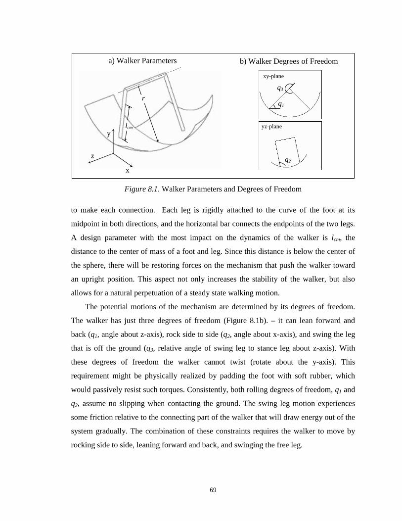
69
Figure 8.1. Walker Parameters and Degrees of Freedom
to make each connection. Each leg is rigidly attached to the curve of the foot at its
midpoint in both directions, and the horizontal bar connects the endpoints of the two legs.
A design parameter with the most impact on the dynamics of the walker islcm, the
distance to the center of mass of a foot and leg. Since this distance is below the center of
the sphere, there will be restoring forces on the mechanism that push the walker toward
an upright position. This aspect not only increases the stability of the walker, but also
allows for a natural perpetuation of a steady state walking motion.
The potential motions of the mechanism are determined by its degrees of freedom.
The walker has just three degrees of freedom (Figure 8.1b). – it can lean forward and
back (q1, angle about z-axis), rock side to side (q2, angle about x-axis), and swing the leg
that is off the ground (q3, relative angle of swing leg to stance leg about z-axis). With
these degrees of freedom the walker cannot twist (rotate about the y-axis). This
requirement might be physically realized by padding the foot with soft rubber, which
would passively resist such torques. Consistently, both rolling degrees of freedom,q1 and
q2, assume no slipping when contacting the ground. The swing leg motion experiences
some friction relative to the connecting part of the walker that will draw energy out of the
system gradually. The combination of these constraints requires the walker to move by
rocking side to side, leaning forward and back, and swinging the free leg.
a) Walker Parameters b) Walker Degrees of Freedom
lcm
r
x
y
z
q1
q2
q3
xy-plane
yz-plane
70
The mechanism’s design is implemented using a simulator. The equations of motion
for the walker are derived using the Euler-Lagrange method. Motion for one stance leg
and one swing leg is then calculated using numerical integration. Through this technique
the simulator accurately computes state transitions according to the dynamic constraints
of the mechanism. The walking system is nonlinear and complex. No analytic control
solution is known.
8.2 The Task Model
In this section, we discuss several elements of the Markov decision process (MDP)
used to model the walking process for reinforcement learning (RL) and develop a model
for learning based on each component. Technically, the underlying task model is not an
MDP due to the discretization of state. Because state in the simulator is continuous, the
discretized MDP state does not represent all of the information about the system, and thus
the system may lose the Markov property. As long as the discretization for the system is
not too severe, the discretized model can be treated as a MDP, although the discrepancy
between real state and modeled state makes it a particularly challenging task for
reinforcement learning. We use two discretizations of the state space: a small model for
experiments in dynamic shaping with a progress estimator, and a larger model to test the
scalability of reward shaping, and its performance in a complex environment.
The MDP of the learning task is denoted M = (S, A, R, T,γ, I). The set of states, S, is
determined by the continuous position and velocities of its three parts. We simplify this
notion of state in two ways. First, the learner may only select an action in those states just
after the walker changes its support leg, which fixesq2 at π/2. Second, we discretize each
state value. For the small model, each angle is limited to four values, and each angular
velocity to five. The larger model allows each angle and velocity to have nine values.
Each discretization uniformly divides the state space. These restrictions result in the final
form of the discretized state vector, Sqqqqqs >∈=< 33211 ,,,, ÿÿÿ .
The action space, A, can apply two torques: T2 applied to rocking (second degree of
freedom), and T3 applied to swinging the free leg (third degree of freedom). For each
action, the rocking torque is applied until rocking velocity is zero, and then the swing
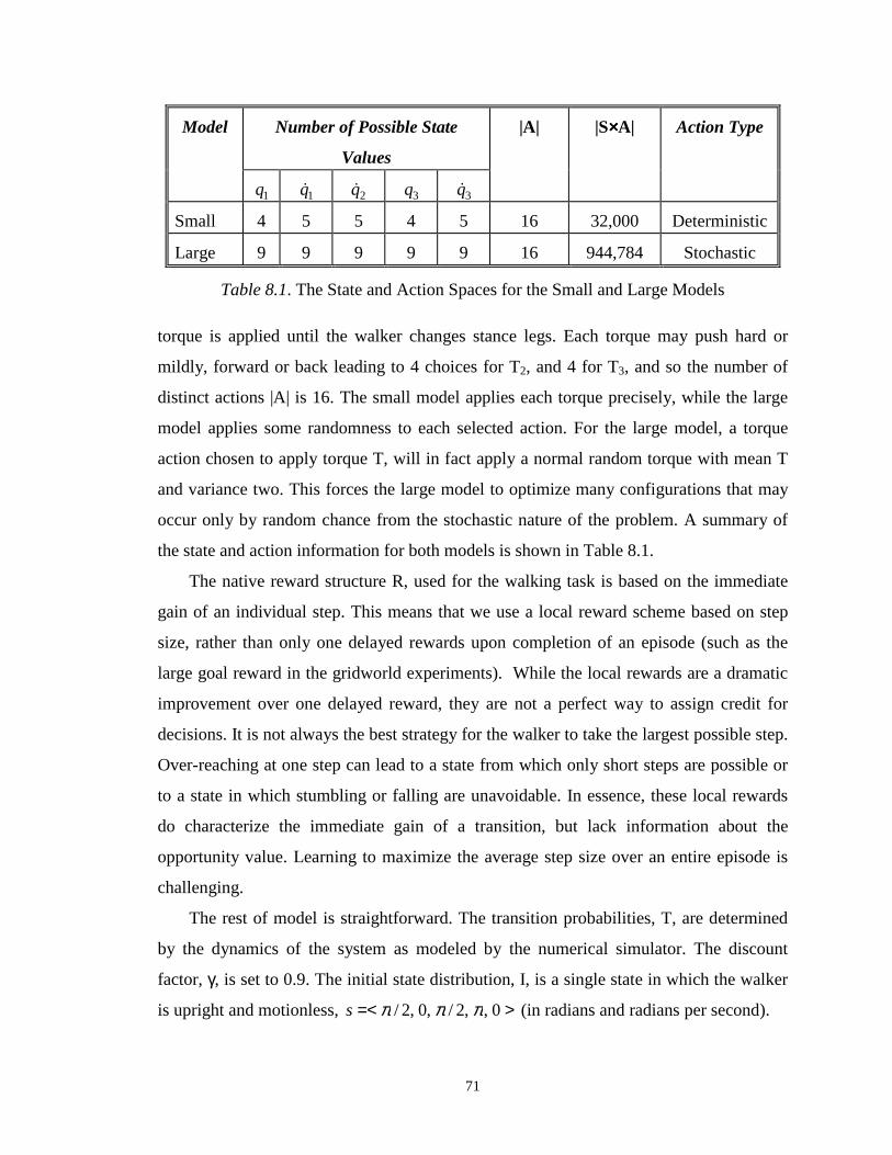
71
Number of Possible State
Values
Model
1q 1qÿ 2qÿ 3q 3qÿ
|A| |S××××A| Action Type
Small 4 5 5 4 5 16 32,000 Deterministic
Large 9 9 9 9 9 16 944,784 Stochastic
Table 8.1. The State and Action Spaces for the Small and Large Models
torque is applied until the walker changes stance legs. Each torque may push hard or
mildly, forward or back leading to 4 choices for T2, and 4 for T3, and so the number of
distinct actions |A| is 16. The small model applies each torque precisely, while the large
model applies some randomness to each selected action. For the large model, a torque
action chosen to apply torque T, will in fact apply a normal random torque with mean T
and variance two. This forces the large model to optimize many configurations that may
occur only by random chance from the stochastic nature of the problem. A summary of
the state and action information for both models is shown in Table 8.1.
The native reward structure R, used for the walking task is based on the immediate
gain of an individual step. This means that we use a local reward scheme based on step
size, rather than only one delayed rewards upon completion of an episode (such as the
large goal reward in the gridworld experiments). While the local rewards are a dramatic
improvement over one delayed reward, they are not a perfect way to assign credit for
decisions. It is not always the best strategy for the walker to take the largest possible step.
Over-reaching at one step can lead to a state from which only short steps are possible or
to a state in which stumbling or falling are unavoidable. In essence, these local rewards
do characterize the immediate gain of a transition, but lack information about the
opportunity value. Learning to maximize the average step size over an entire episode is
challenging.
The rest of model is straightforward. The transition probabilities, T, are determined
by the dynamics of the system as modeled by the numerical simulator. The discount
factor,γ, is set to 0.9. The initial state distribution, I, is a single state in which the walker
is upright and motionless, >=< 0,,2/,0,2/ πππs (in radians and radians per second).
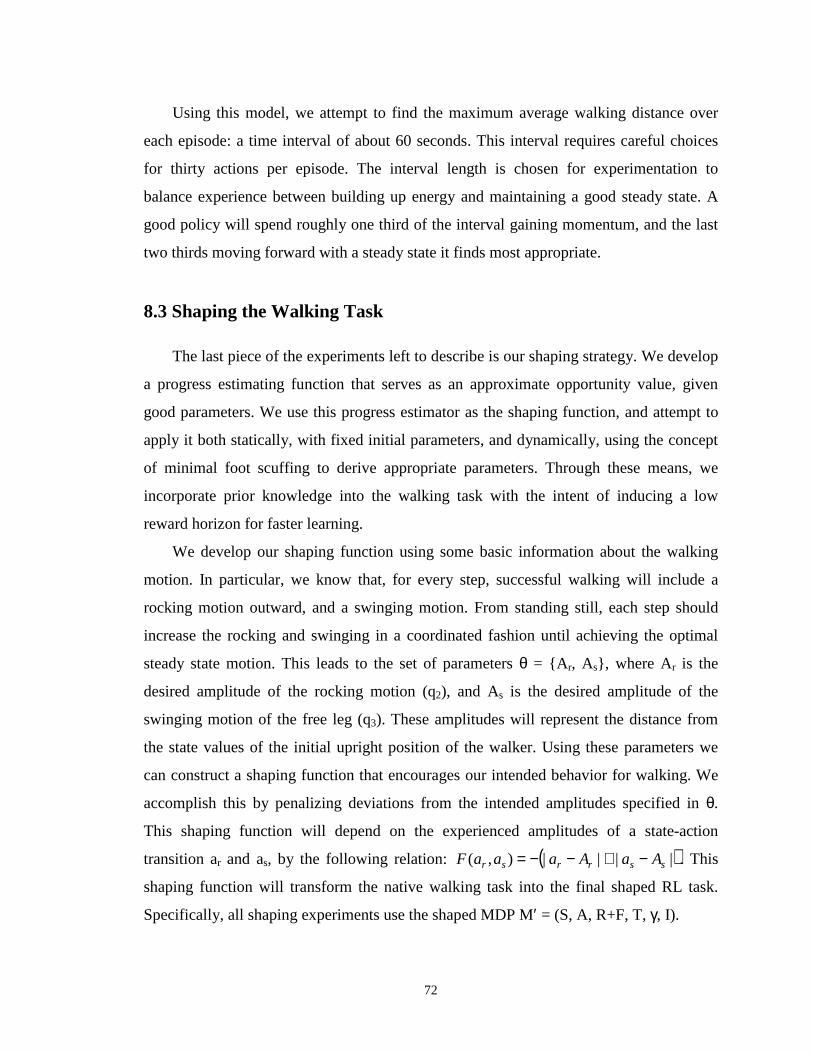
72
Using this model, we attempt to find the maximum average walking distance over
each episode: a time interval of about 60 seconds. This interval requires careful choices
for thirty actions per episode. The interval length is chosen for experimentation to
balance experience between building up energy and maintaining a good steady state. A
good policy will spend roughly one third of the interval gaining momentum, and the last
two thirds moving forward with a steady state it finds most appropriate.
8.3 Shaping the Walking Task
The last piece of the experiments left to describe is our shaping strategy. We develop
a progress estimating function that serves as an approximate opportunity value, given
good parameters. We use this progress estimator as the shaping function, and attempt to
apply it both statically, with fixed initial parameters, and dynamically, using the concept
of minimal foot scuffing to derive appropriate parameters. Through these means, we
incorporate prior knowledge into the walking task with the intent of inducing a low
reward horizon for faster learning.
We develop our shaping function using some basic information about the walking
motion. In particular, we know that, for every step, successful walking will include a
rocking motion outward, and a swinging motion. From standing still, each step should
increase the rocking and swinging in a coordinated fashion until achieving the optimal
steady state motion. This leads to the set of parametersθ = {A r, As}, where Ar is the
desired amplitude of the rocking motion (q2), and As is the desired amplitude of the
swinging motion of the free leg (q3). These amplitudes will represent the distance from
the state values of the initial upright position of the walker. Using these parameters we
can construct a shaping function that encourages our intended behavior for walking. We
accomplish this by penalizing deviations from the intended amplitudes specified inθ.
This shaping function will depend on the experienced amplitudes of a state-action
transition ar and as, by the following relation: ( )||||),( ssrrsr AaAaaaF −+−−= . This
shaping function will transform the native walking task into the final shaped RL task.
Specifically, all shaping experiments use the shaped MDP M′ = (S, A, R+F, T,γ, I).
73
Parameter Set Ar (radians) As (radians)
Control .15 1.02
Small .05 .2
Medium .1 .5
Large .3 1.2
Table 8.2. Shaping Parameter Sets
Given this form of the shaping function, we must select values for the desired rock
and swing amplitudes, Ar and As. For static shaping we must specify these values directly
from domain knowledge. For the purposes of comparison, we obtain an ideal set of
values by first training a walking policy without shaping. We then extract the amplitudes
from the behavior of the best learned policy. We refer to these values as the control
parameters (Table 8.2). Of course, it is unrealistic in general to require these values, but
they are useful for comparison.
Realistically, we can expect only approximations, which, while perhaps inaccurate,
may enhance learning through shaping. We explore three such estimates. To choose their
values, we notice the fact that the fastest walking occurs by taking the largest step
possible in the time between collisions with the ground. This premise indicates a
dependence on the period of the rocking motion. If the period can be driven to a short
interval, the fastest walking may be several short steps. If the rocking period is long
regardless of the action executed, we expect large steps to be effective. If the action set
allows for partial control of the period, the best course of actions could be medium
optimally timed steps. Based on these ideas, and knowledge of the range of reasonable
values for the rocking and swinging amplitudes, we define the parameter sets shown in
Table 8.2. Using these values, we can apply the amplitude-critic shaping function
statically.
For dynamic shaping, we apply the progress estimator approach from Chapter 6 to
handle parameter adjustment and shaping integration. Parameter adjustment is carried out
using simple domain knowledge, which applies qualitative rules to the all the experience
observed so far. The qualitative constraints for walking can be attained by a simple
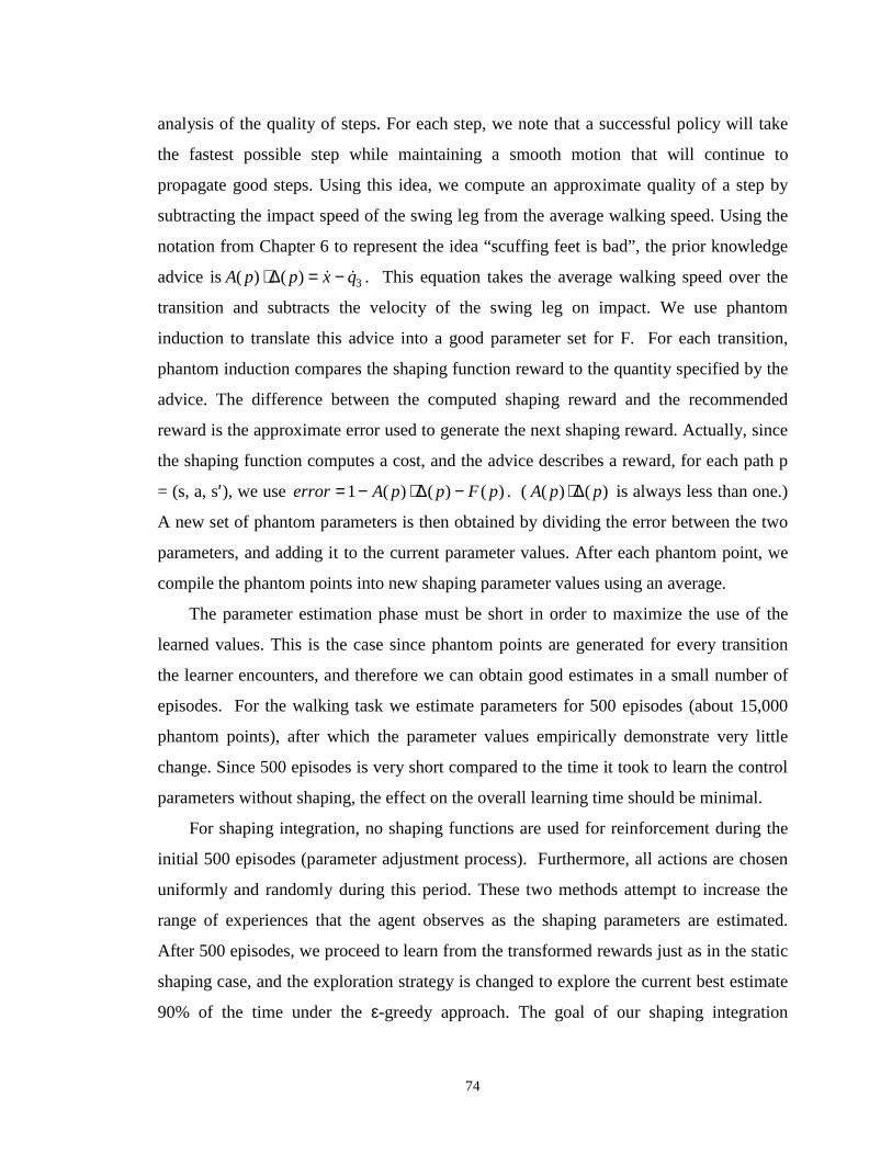
74
analysis of the quality of steps. For each step, we note that a successful policy will take
the fastest possible step while maintaining a smooth motion that will continue to
propagate good steps. Using this idea, we compute an approximate quality of a step by
subtracting the impact speed of the swing leg from the average walking speed. Using the
notation from Chapter 6 to represent the idea “scuffing feet is bad”, the prior knowledge
advice is 3)()( qxppA ÿÿ −=∆⋅ . This equation takes the average walking speed over the
transition and subtracts the velocity of the swing leg on impact. We use phantom
induction to translate this advice into a good parameter set for F. For each transition,
phantom induction compares the shaping function reward to the quantity specified by the
advice. The difference between the computed shaping reward and the recommended
reward is the approximate error used to generate the next shaping reward. Actually, since
the shaping function computes a cost, and the advice describes a reward, for each path p
= (s, a, s′), we use )()()(1 pFppAerror −∆⋅−= . ( )()( ppA ∆⋅ is always less than one.)
A new set of phantom parameters is then obtained by dividing the error between the two
parameters, and adding it to the current parameter values. After each phantom point, we
compile the phantom points into new shaping parameter values using an average.
The parameter estimation phase must be short in order to maximize the use of the
learned values. This is the case since phantom points are generated for every transition
the learner encounters, and therefore we can obtain good estimates in a small number of
episodes. For the walking task we estimate parameters for 500 episodes (about 15,000
phantom points), after which the parameter values empirically demonstrate very little
change. Since 500 episodes is very short compared to the time it took to learn the control
parameters without shaping, the effect on the overall learning time should be minimal.
For shaping integration, no shaping functions are used for reinforcement during the
initial 500 episodes (parameter adjustment process). Furthermore, all actions are chosen
uniformly and randomly during this period. These two methods attempt to increase the
range of experiences that the agent observes as the shaping parameters are estimated.
After 500 episodes, we proceed to learn from the transformed rewards just as in the static
shaping case, and the exploration strategy is changed to explore the current best estimate
90% of the time under theε-greedy approach. The goal of our shaping integration
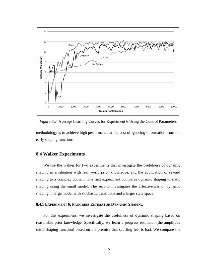
75
Figure 8.2. Average Learning Curves for Experiment 6 Using the Control Parameters
methodology is to achieve high performance at the cost of ignoring information from the
early shaping functions.
8.4 Walker Experiments
We use the walker for two experiments that investigate the usefulness of dynamic
shaping in a situation with real world prior knowledge, and the application of reward
shaping to a complex domain. The first experiment compares dynamic shaping to static
shaping using the small model. The second investigates the effectiveness of dynamic
shaping in large model with stochastic transitions and a larger state space.
8.4.1 EXPERIMENT 6: PROGRESSESTIMATOR DYNAMIC SHAPING
For this experiment, we investigate the usefulness of dynamic shaping based on
reasonable prior knowledge. Specifically, we learn a progress estimator (the amplitude
critic shaping function) based on the premise that scuffing feet is bad. We compare the
0
2
4
6
8
10
12
14
0 1000 2000 3000 4000 5000 6000 7000 8000 9000 10000
Number of Episodes
Dis
tanc
eW
alke
d(m
)
No Shape
Dynamic
Static
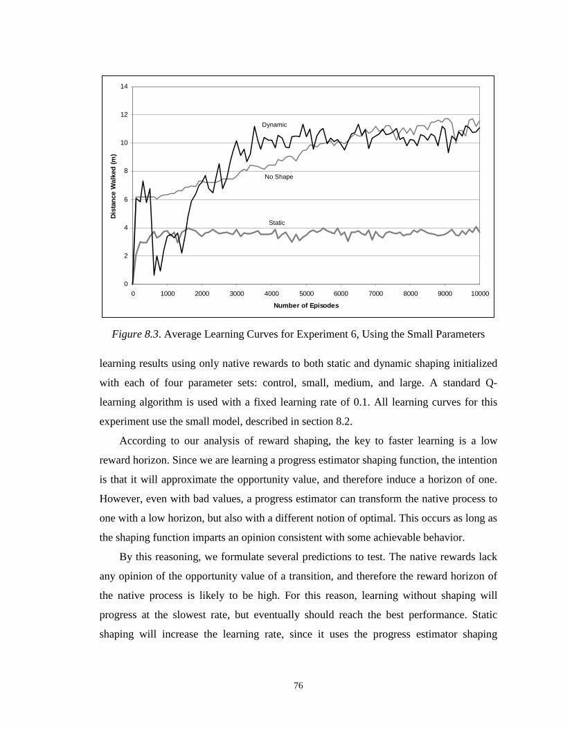
76
Figure 8.3. Average Learning Curves for Experiment 6, Using the Small Parameters
learning results using only native rewards to both static and dynamic shaping initialized
with each of four parameter sets: control, small, medium, and large. A standard Q-
learning algorithm is used with a fixed learning rate of 0.1. All learning curves for this
experiment use the small model, described in section 8.2.
According to our analysis of reward shaping, the key to faster learning is a low
reward horizon. Since we are learning a progress estimator shaping function, the intention
is that it will approximate the opportunity value, and therefore induce a horizon of one.
However, even with bad values, a progress estimator can transform the native process to
one with a low horizon, but also with a different notion of optimal. This occurs as long as
the shaping function imparts an opinion consistent with some achievable behavior.
By this reasoning, we formulate several predictions to test. The native rewards lack
any opinion of the opportunity value of a transition, and therefore the reward horizon of
the native process is likely to be high. For this reason, learning without shaping will
progress at the slowest rate, but eventually should reach the best performance. Static
shaping will increase the learning rate, since it uses the progress estimator shaping
0
2
4
6
8
10
12
14
0 1000 2000 3000 4000 5000 6000 7000 8000 9000 10000
Number of Episodes
Dis
tanc
eW
alke
d(m
)
No Shape
Dynamic
Static
77
Figure 8.4. Average Learning Curves for Experiment 6, Using the Medium Parameters
function. However, it will likely reach sub-optimal performance when not using the
control-condition parameter values. Dynamic shaping, regardless of the parameter set,
will quickly reach performance near the no-shaping learner, but only after the parameter
estimation period in which performance may be quite poor.
Figures 8.2-8.5 illustrate the results of the shaping techniques using different initial
parameters (Static & Dynamic), compared to learning from only native rewards (No
Shape). Each graph plots the performance of following the policy learned after a given
number of episodes, not the performance achieved during training. All learning curves
are average data from 10 trials. Each test is carried out for 10,000 episodes.
A summary of this information is shown in Figure 8.6, which displays the average
interval performances and their 95% confidence intervals. Here all the data from intervals
of 2000 episodes are averaged. Figure 8.6 displays the learning curves in a corresponding
progression of columns representing each interval.
For comparison, we begin learning to walk without the use of shaping. The total
distance walked jumps rapidly to about 6m, highlighting the benefits of the local step size
rewards. The result of the step size feedback is a stumbling, forward movement. The
0
2
4
6
8
10
12
14
0 1000 2000 3000 4000 5000 6000 7000 8000 9000 10000
Number of Episodes
Dis
tanc
eW
alke
d(m
)
Static
Dynamic
No Shape
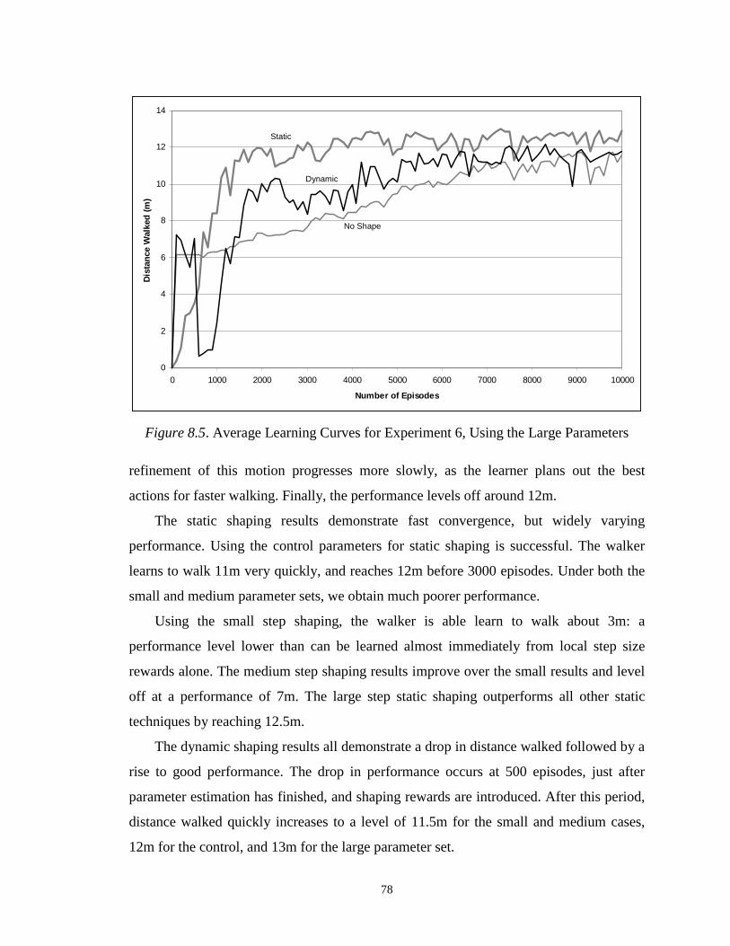
78
Figure 8.5. Average Learning Curves for Experiment 6, Using the Large Parameters
refinement of this motion progresses more slowly, as the learner plans out the best
actions for faster walking. Finally, the performance levels off around 12m.
The static shaping results demonstrate fast convergence, but widely varying
performance. Using the control parameters for static shaping is successful. The walker
learns to walk 11m very quickly, and reaches 12m before 3000 episodes. Under both the
small and medium parameter sets, we obtain much poorer performance.
Using the small step shaping, the walker is able learn to walk about 3m: a
performance level lower than can be learned almost immediately from local step size
rewards alone. The medium step shaping results improve over the small results and level
off at a performance of 7m. The large step static shaping outperforms all other static
techniques by reaching 12.5m.
The dynamic shaping results all demonstrate a drop in distance walked followed by a
rise to good performance. The drop in performance occurs at 500 episodes, just after
parameter estimation has finished, and shaping rewards are introduced. After this period,
distance walked quickly increases to a level of 11.5m for the small and medium cases,
12m for the control, and 13m for the large parameter set.
0
2
4
6
8
10
12
14
0 1000 2000 3000 4000 5000 6000 7000 8000 9000 10000
Number of Episodes
Dis
tanc
eW
alke
d(m
)Static
Dynamic
No Shape
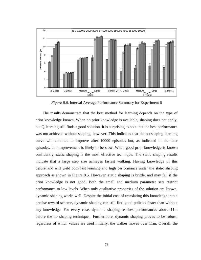
79
Figure 8.6. Interval Average Performance Summary for Experiment 6
The results demonstrate that the best method for learning depends on the type of
prior knowledge known. When no prior knowledge is available, shaping does not apply,
but Q-learning still finds a good solution. It is surprising to note that the best performance
was not achieved without shaping, however. This indicates that the no shaping learning
curve will continue to improve after 10000 episodes but, as indicated in the later
episodes, this improvement is likely to be slow. When good prior knowledge is known
confidently, static shaping is the most effective technique. The static shaping results
indicate that a large step size achieves fastest walking. Having knowledge of this
beforehand will yield both fast learning and high performance under the static shaping
approach as shown in Figure 8.5. However, static shaping is brittle, and may fail if the
prior knowledge is not good. Both the small and medium parameter sets restrict
performance to low levels. When only qualitative properties of the solution are known,
dynamic shaping works well. Despite the initial cost of translating this knowledge into a
precise reward scheme, dynamic shaping can still find good policies faster than without
any knowledge. For every case, dynamic shaping reaches performances above 11m
before the no shaping technique. Furthermore, dynamic shaping proves to be robust;
regardless of which values are used initially, the walker moves over 11m. Overall, the
0
2
4
6
8
10
12
14
No Shape Small Medium Large Control Small Medium Large Control
Dis
tanc
eW
alke
d(m
)
0-1900 2000-3900 4000-5900 6000-7900 8000-10000
Static Dynamic
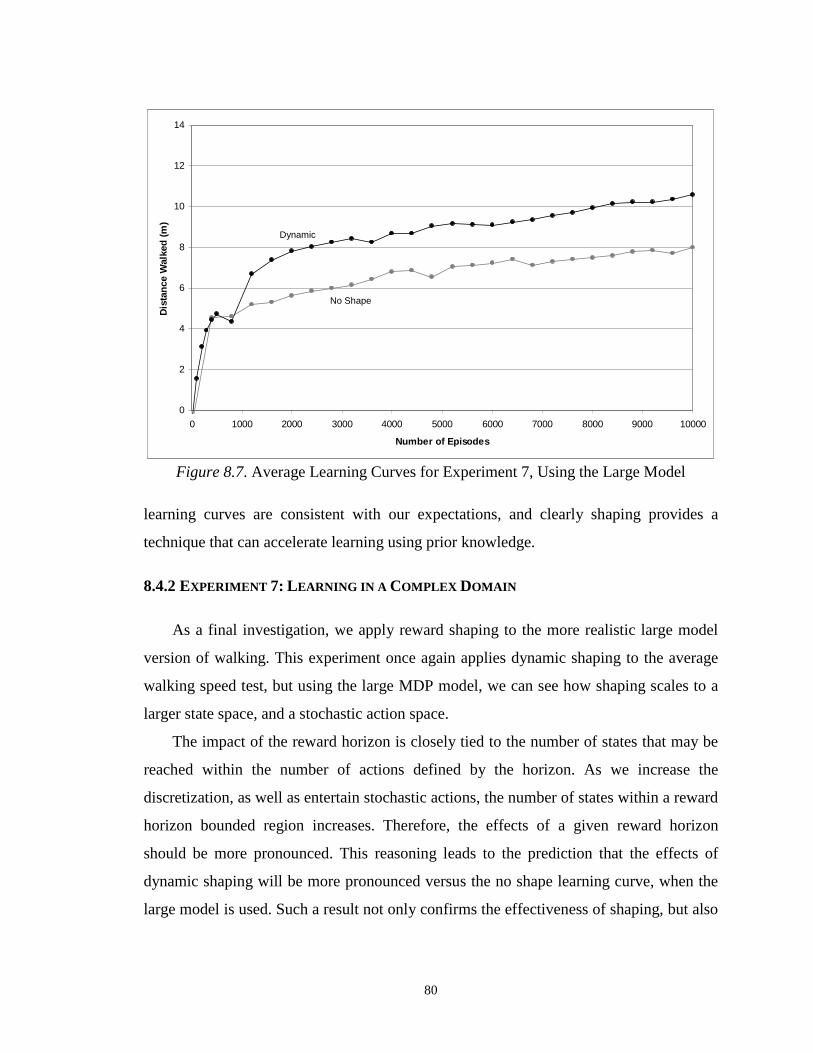
80
0
2
4
6
8
10
12
14
0 1000 2000 3000 4000 5000 6000 7000 8000 9000 10000
Number of Episodes
Dis
tanc
eW
alke
d(m
)
Figure 8.7. Average Learning Curves for Experiment 7, Using the Large Model
learning curves are consistent with our expectations, and clearly shaping provides a
technique that can accelerate learning using prior knowledge.
8.4.2 EXPERIMENT 7: LEARNING IN A COMPLEX DOMAIN
As a final investigation, we apply reward shaping to the more realistic large model
version of walking. This experiment once again applies dynamic shaping to the average
walking speed test, but using the large MDP model, we can see how shaping scales to a
larger state space, and a stochastic action space.
The impact of the reward horizon is closely tied to the number of states that may be
reached within the number of actions defined by the horizon. As we increase the
discretization, as well as entertain stochastic actions, the number of states within a reward
horizon bounded region increases. Therefore, the effects of a given reward horizon
should be more pronounced. This reasoning leads to the prediction that the effects of
dynamic shaping will be more pronounced versus the no shape learning curve, when the
large model is used. Such a result not only confirms the effectiveness of shaping, but also
Dynamic
No Shape
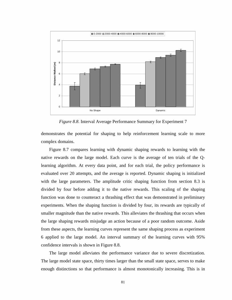
81
Figure 8.8. Interval Average Performance Summary for Experiment 7
demonstrates the potential for shaping to help reinforcement learning scale to more
complex domains.
Figure 8.7 compares learning with dynamic shaping rewards to learning with the
native rewards on the large model. Each curve is the average of ten trials of the Q-
learning algorithm. At every data point, and for each trial, the policy performance is
evaluated over 20 attempts, and the average is reported. Dynamic shaping is initialized
with the large parameters. The amplitude critic shaping function from section 8.3 is
divided by four before adding it to the native rewards. This scaling of the shaping
function was done to counteract a thrashing effect that was demonstrated in preliminary
experiments. When the shaping function is divided by four, its rewards are typically of
smaller magnitude than the native rewards. This alleviates the thrashing that occurs when
the large shaping rewards misjudge an action because of a poor random outcome. Aside
from these aspects, the learning curves represent the same shaping process as experiment
6 applied to the large model. An interval summary of the learning curves with 95%
confidence intervals is shown in Figure 8.8.
The large model alleviates the performance variance due to severe discretization.
The large model state space, thirty times larger than the small state space, serves to make
enough distinctions so that performance is almost monotonically increasing. This is in
0
2
4
6
8
10
12
No Shape Dynamic
Dis
tanc
eW
alke
d(m
)
0-2000 2000-4000 4000-6000 6000-8000 8000-10000
82
contrast to the jagged learning curves in experiment seven, and is most likely due to
transition dynamics that much more closely approximate a Markov process. That is,
because the state space is more refined, the optimal action for each state is less
dependent, if at all, on an extended history of previous transitions.
Dynamic shaping outperforms conventional reinforcement learning. After 10,000
training episodes, the no shape learner reaches an average performance of under 8m. On
the other hand, the dynamic shaping curve achieves a performance over 10m, which is
not far off from its typical performance in the simple model. Figure 8.8, shows that after
the first interval, dynamic shaping has an average performance significantly greater than
the performance achieved without shaping. In fact the shaped system outperforms the
best non-shaped policy after only 2000 training episodes. While the effects of the larger
state space and stochastic actions reduce the learning rates in each case, the fact that
dynamic shaping still reaches a high level of performance demonstrates the ability of
shaping to extend reinforcement learning to more complex domains.

83
CHAPTER9
Related Work
Several works have provide a strong background and motivation for our work on
reward shaping. This work is primarily in three areas: shaping applications, potential-
based shaping, and other approaches that shape learning without using rewards.
9.1 Empirical Successes with Shaping
Many related works describe the success of shaping through experimentation in
various domains. Each work gives valuable insight into the workings of reward shaping
and presents experiments that demonstrate the value of shaping.
Shaping has been used to train robots to conform to intended behaviors. Dorigo and
Colombetti [1993] train a small mobile robot to perform desired behaviors using shaping.
They describe their approach as supervised reinforcement learning, and advance this idea
as a means of translating suggestions from an external trainer into a desirable control
strategy. Saksida, Raymond, and Touretzky [1998] use the idea of shaping to train a
mobile robot. The authors use a technique for shaping based in animal learning theory,
and promote behavior editing as an underlying mechanism to the shaping process.
Other work focuses directly on modifying the reward structure to enhance the
learning process. Mataric [1994] trains multiple robots in a foraging task. She describes
two ways of enhancing rewards for accelerated learning: using progress estimators, and
reinforcing multiple goals. These ideas are some of the motivating factors in the
development of our subgoal shaping techniques. Randløv and Alstrøm [1998] use a
84
shaping function to learn a control policy for riding a bicycle to a goal. The shaping
function provides local feedback that rewards progress toward the goal. The authors
hand-tune the function in order to achieve an appropriate tradeoff between balance and
direction. The need to hand-tune the shaping function led to our research on dynamic
shaping.
9.2 Potential-Based Shaping
The addition of shaping rewards changes the Markov decision process (MDP) to be
solved. Integrating strong advice into a system can accelerate learning, but if the advice is
inaccurate, the resulting policy will demonstrate less than optimal behavior. However,
this transformation need not alter the optimal policy. Ng, Harada, and Russell [1999]
show necessary and sufficient conditions for a policy to remain optimal under addition of
a shaping reward structure. They, like other shaping investigators, demonstrate
accelerated learning empirically, but specify no analytical results along these lines. The
question of what sort of shaping policy will speed rather than delay convergence to the
optimal policy is left largely unanalyzed. The empirical tests from this work lay the
foundation for the stochastic gridworld problem, and suggest that state utilities be used as
the shaping potential. These results motivated the concept of opportunity value for
inducing a reward horizon as an answer to both faster learning, and preserving the
optimal policy.
Potential functions over the state space do not allow the flexibility of action-based
shaping rewards. Wiewiora, Cottrell, and Elkan [2003] extend the idea of potential-based
shaping to offer advice about actions as well as states. They suggest using a potential
field over the combined state-action space. The shaping function becomes the difference
between two state actions, and therefore requires four inputs. Since a transition does not
specify the two actions that they require to compute the difference in potentials, the
authors propose two strategies: look-ahead, and look-back advice. Both types of advice
are shown to preserve the ordering of Q-values, and empirically demonstrate accelerated
learning.
85
9.3 Shaping Without Rewards
There are hierarchical approaches to reinforcement learning, which aim to organize a
complex behavior into a hierarchy of dependent, but simpler sub-tasks. Two of the works
in this area are hierarchical EBRL [Tadepalli & Dietterich, 1997] and the MAXQ
algorithm [Dietterich, 2000]. Hierarchical reinforcement learning build behaviors that
work together to successively approximate a desired behavior. In that sense, it follows the
same motivation as reward shaping, but with a different methodology.
Another alternative to dealing explicitly with rewards is to identify definite points of
progress, and implement mechanisms to reach these subgoals. McGovern and Barto
[2001] present a method to automatically detect subgoals, and to take advantage of the
subgoals by using policies as macro actions, or options. Similarly, Goel and Huber [2003]
apply the same process of subgoal identification and macro actions to the hierarchical
reinforcement learning paradigm. While not directly changing the rewards of the problem
while training, these techniques derive the macro actions via learning in a separate
process, where the reaching the subgoal generates the highest return. The idea of
subgoals ties in closely with the concept of inducing a low reward horizon, and therefore
conditioning a learner with localized feedback.
Other methods mold the learning process by incorporating prior beliefs into the state
and action representations. Even-Dar, Mannor, and Mansour [2003] outline an algorithm
to eliminate actions from consideration when warranted by experience in the domain. By
automatically, and appropriately reducing the size of the action space, they are able to
demonstrate faster learning and a good final policy. Sutton, Precup, and Singh [1999]
introduce the idea of relativized options: related macro actions can implement a simple
behavior in among many related tasks. Relativized options can alleviate the
complications of larger state spaces by suggesting macro actions that apply to
homomorphic regions of states. Other techniques share information between states by
using utility function approximators [Tesauro, 1992; Bertsekas and Tsitsiklis, 1996].
86
CHAPTER10
Future Work
We have written, to the best of our knowledge, the first theory of reward shaping that
explains why learning is accelerated through rewards, and describes the ideal information
that shaping rewards should attempt to convey. These results lay the foundation for the
development of successful shaping techniques. Our work on subgoal shaping and
progress estimators is a first attempt to establish such techniques, but it also highlights
several areas to explore further, including shaping reward functions, dynamic shaping
algorithms, and reinforcement learning algorithms more receptive to shaping.
10.1 Shaping Reward Functions
Our work emphasizes the importance of subgoals and progress estimators for
successful shaping functions. However, neither utility subgoals, nor approximate
subgoals were able to scale very far as prior knowledge accuracy was reduced. As the
underlying horizon that was imposed by these methods in experiments three and four
increased, shaping error began to dominate, and learning time was not reduced as
effectively as it could have been (experiment 1). This not only invites research on how to
scale these subgoal techniques, but also suggests that there is room for improvement in
the design of shaping functions overall.
As the distance between subgoals increases in a stochastic environment, the
likelihood of traveling directly from one subgoal to the next decreases. This property
explains why shaping error begins to affect the learning process at higher horizons when
87
using simple subgoal techniques. For example, the approximate subgoal potential
function shown in Figure 7.9 uses very few subgoals. While it does encourage the correct
policy within the reward horizon, the expected net gain for following this policy
decreases as the horizon increases. This effect is due to randomness in the environment:
even the best policy has a decreasing probability of reaching that subgoal state as it
moves farther away. An approach is needed that can apply the limited prior knowledge
used by the subgoal shaping techniques to “blanket” an area of important subgoal states
with approximate values such that the best decision is made clear regardless of the
horizon size. Solving this problem will allow shaping to scale up to its potential, as
indicated in experiment one, so that even a subgoal near the final goal state can have an
impact.
There is also evidence to support the investigation of other types of shaping rewards.
The amplitude-critic shaping function from the walking experiments demonstrates
accelerated learning of a good policy, and does not directly involve subgoals or a
potential-based structure. Moreover, while opportunity value can be represented as a
potential function, scaled opportunity value cannot. This is a consequence of including
native reward feedback which inherently depends on actions. We refer to shaping
functions that are not potential based, but still attempt to approximate opportunity value
on every transition as progress estimators. Many useful research topics are relevant here,
such as an investigation on useful types of progress estimator functions, a look at
progress estimators that can withhold an opinion for some transitions, and combinations
of progress estimators based on different prior knowledge.
10.2 Dynamic Shaping
The case for dynamic shaping is also divided between potential-based shaping and
progress estimator shaping. We motivate, present, and demonstrate two dynamic shaping
techniques based on these ideas. There are interesting extensions to these approaches as
well as possibilities for alternative methods.
One interesting extension for potential function dynamic shaping is to represent the
potential field as a function that can generalize over states rather than a tabular approach.
88
Similar to the idea of a value function approximator, such as neural nets, the potential
function approximator could represent the potential field values in a parameter space with
a size lower than the size of the state space. Even when the utilities are not approximated
by a function, it is useful to do so for the potential function because a smaller parameter
space could lead to faster learning. And quick convergence is of critical importance for
dynamic shaping. Therefore examining potential function approximators to find those
that provide acceptable accuracy with decreased learning time could have significant
impact to the dynamic shaping process overall.
There are also alternative methods for dynamic shaping. Although we suggest two
techniques, the fundamental process of dynamic shaping – learning the shaping function
through initial experiences of the task – has many possibilities. Of primary interest are
dynamic learning processes that work with any type of shaping function. Our results in
dynamic shaping currently depend on the type of shaping function: potential-based, or
progress estimator. It is valuable to consider refinements of dynamic shaping to these
types of functions, extensions of dynamic shaping to new shaping functions, and even
dynamic shaping that will work independent to the category of shaping function being
used.
10.3 Shaping-Responsive Learning
The experimental work in this paper uses the conventional Q-learning algorithm with
ε-greedy exploration. There are many advantages to this algorithm. Q-learning is
responsive to the reward horizon without requiring it as an input. Furthermore,ε-greedy
requires no overhead to plan its course of exploration. However, the Horizon-Learn
algorithm suggests that other learning algorithms may be more responsive to shaping if
they can focus all exploration into regions warranted by the reward horizon. Horizon-
Learn develops conditions that judge a state a known, which has the power to eliminate
all further exploration from that state.
Combining the ability of Horizon-Learn to make accurate snap judgments with the
simple effectiveness of Q-learning may lead to the development of a shaping-responsive
learner. The intent is that by explicitly designing the idea of the reward horizon into a

89
utility value reinforcement learner, it may become more sensitive to shaping advice, and
enhance the speedup and scalability even further from what we demonstrate in this paper.
While explicit use of the horizon can potentially improve speed over that of Q-learning, it
is not a trivial input to require. A powerful result would be to find a learning algorithm
that performs exploration by using a successively expanding horizon, when it is becomes
clear through experience that lower horizons are inconsistent with good global
performance.
90
CHAPTER11
Conclusion
We have written a theory of reward shaping that explains the ability of reward
shaping to accelerate the learning process. Central to this work is the concept of a reward
horizon: the delay between an action and an accurate judgment of its effects on a global
scale. This idea is not surprising when viewed in light of the conditioning process from
psychology. Many forms of life learn a causal structure of their environment based on
associations of an unconditional stimulus to other events, or their own behavior. We have
placed this idea within the computational framework of reinforcement learning, and
proven that the strength of that association, the reward horizon, plays the integral role in
determining the learning rate of a behavior in a given environment.
One type of feedback that generates an ideal learning environment is opportunity
value. Opportunity value is the value of the resultant state of an action minus the value of
the initial state. It describes how much better it is to be in the position that resulted from
an action rather than to have not moved at all. Opportunity value is the complementary
information to rewards. While rewards describe the immediate gain of an action,
opportunity value describes the progress on a global scale. Because of this property,
opportunity value is the ideal shaping reward: it induces a reward horizon of one, and
preserves the optimal policy.
The challenge for reward shaping is to convey the available prior knowledge in a
manner that will accelerate learning, but not deteriorate final performance. Opportunity
value is the ideal candidate, but requires complete and perfect knowledge of the state
utilities for the reinforcement learning task. To avoid this unreasonable prerequisite, we

91
propose the ideas of subgoal shaping and dynamic shaping. Subgoal shaping gives extra
reinforcement to subgoals states that are known to have some relative benefit or
detriment to the intended behavior. By this process, subgoal shaping allows for
accelerated learning when any prior knowledge is available, even if it is incomplete and
imperfect. Dynamic shaping is a further aid in translating limited prior knowledge into an
augmented reward structure. Dynamic shaping pairs the task of learning appropriate
shaping reward values with the task of finding the optimal behavior. Through the use of
an additional learning task, prior knowledge is freed from the necessity to formulate
precise values. Instead, prior knowledge can be used on a qualitative level to drive the
dynamic shaping process toward a useful augmentation of the native reward by using
experience in the domain.
The theory in this paper presents a complete methodology to effectively
communicate prior knowledge to a reinforcement learning agent and provides guarantees
of its effects on the learning rate and final performance. All aspects of the theory hold up
to experimentation in a stochastic gridworld. Moreover, dynamic shaping allows
reinforcement learning to tackle the challenging task of bipedal walking efficiently, even
with a complex model of the domain. The potential for using shaping advice to condition
intended behaviors is apparent in both theory, and application.

92
Bibliography
[Abramowitz & Stegun, 1972] Abramowitz and Stegun. (1972).Handbook of
Mathematical Functions, 9th edition. Dover Publications, New York.
[Bertsekas & Tsitsiklis, 1996] Bertsekas, D. P., and Tsitsiklis J. N. (1996)Neurodynamic
Programming. Athena Scientific.
[Bradtke & Duff, 1995] Bradtke, S. J., and Duff, M.O. (1995). Reinforcement Learning
Methods for Continuous-Time Markov Decision Problems. In G. Tesauro, D. S.
Touretzky, and T. K. Leen, (Eds.).Advances in Neural Information Processing
Systems 7. MIT Press, Cambridge, MA.
[Brafman & Tennenholtz, 2002] Brafman, R., and Tennenholtz, M. (2002). R-MAX – A
General Polynomial Time Algorithm for Near-Optimal Reinforcement Learning.
Journal of Machine Learning Research, 3, 213-231.
[Brodie & DeJong, 1998] Brodie, M., and DeJong G. (1998). Iterated Phantom Induction:
A Little Knowledge Can Go a Long Way.Proceedings of Fifteenth National
Conference on Artificial Intelligence(pp. 665-670). AAAI Press, Menlo Park, CA.
[Cover & Thomas, 1991] Cover, T. M. and Thomas, J. A. (1991)Elements of Information
Theory. John Wiley and Sons, Inc., NY.
93
[Crites & Barto, 1996] Crites, R.H., and Barto, A.G. (1996). Improving elevator
performance using reinforcement learning. In D.S. Toouretzky, M.C. Mozer, and M.
E. Hasselmo (eds.),Advances in Neural Information Processing Systems:
Proceedings of the 1995 Conference(pp. 1017-1023). MIT Press, Cambridge, MA.
[Dietterich, 2000] Dietterich, T. (2000) Hierarchical Reinforcement Learning with the
MAXQ Value Function Decomposition.Journal of Artificial Intelligence Research,
12, 227-303.
[Dorigo & Colombetti, 1993] Dorigo, M., and Colombetti, M. (1993)Robot Shaping:
Developing Situated Agents through Learning.Technical Report TR-92-040,
International Computer Science Institute, Berkeley, CA.
[Evan-Dar et al, 2003] Evan-Dar, E., Mannor, S., and Mansour, Y. (2003) Action
elimination and stopping conditions for reinforcement learning.Proceedings of the
Twentieth International Conference on Machine Learning. AAAI Press, CA.
[Garcia et al, 1998] Garcia, M., Chatterjee, A., Ruina, A., and Coleman, M. (1998). The
simplest walking model: Stability, complexity, and scaling.Journal of
Biomechanical Engineering. v120, 281-288. ASME, USA.
[Goel & Huber, 2003] Goel, S. and Huber, M. (2003) Subgoal discovery for hierarchical
reinforcement learning using learned policies.Proceedings of the Sixteenth
International FLAIRS Conference. (pp. 346-350).
[Hogg & Tanis, 2001] Hogg and Tanis. (2001).Probability and Statistical Inference.
Prentice-Hall, New Jersey.
[Kaelbling et al, 1996] Kaelbling, L., Littman, L., and Moore, A. (1996). Reinforcement
learning: a survey.Journal of Artificial Intelligence Research. v4, 237-285.
[Kearns & Singh, 1998] Kearns and Singh. (1998) Near-optimal reinforcement learning
in polynomial time. Proceedings of the Fifteenth International Conference on
Machine Learning(pp. 260-268). Morgan Kaufmann, CA.
94
[Laud & DeJong, 2002] Laud and DeJong. (2002). Reinforcement Learning and Shaping:
Encouraging Intended Behaviors.Proceedings of the Nineteenth International
Conference on Machine Learning(pp. 355-362). Morgan Kaufmann, CA.
[Laud & Dejong, 2003] Laud and DeJong. (2003). The influence of reward on the speed
of reinforcement learning: an analysis of shaping.Proceedings of the Twentieth
International Conference on Machine Learning(pp. 355-362). Morgan Kaufmann,
CA.
[Mackintosh, 1999] Mackintosh, N. (1999) Conditioning. In Wilson, R. A., and Keil, F.
C. (eds.)The MIT Encyclopedia of the Cognitive Sciences(pp. 182-183). MIT Press,
MA.
[Mataric, 1994] Mataric, M. J. (1994). Reward functions for accelerated learning. In
Cohen, W. W. and Hirsh, H. (Eds.).Proceedings of the Eleventh International
Conference on Machine Learning. Morgan Kaufmann, CA.
[McGovern & Barto, 2001] McGovern, A., Barto, A.G. (2001) Automatic discovery of
subgoals in reinforcement learning using diverse density.Proceedings of the
Eighteenth International Conference on Machine Learning.(pp. 361—368). Morgan
Kaufmann, CA.
[Mitchell, 1997] Mitchell, T. M. (1997)Machine Learning. McGraw-Hill, MA.
[Ng et al, 1999] Ng, A., Harada, D., & Russell, S. (1999). Policy invariance under reward
transformations: Theory and application to reward shaping.Proceedings of the
Sixteenth International Conference on Machine Learning. Bled, Slovenia: Morgan
Kaufmann.
[Press et al, 1988] Press W., Flannery B., Teukolsky S., and Vetterling W. (1988).
Numerical Recipes in C. Cambridge University Press, Cambridge.
[Randløv & Alstrøm, 1998] Randløv, J., and Alstrøm, P. (1998). Learning to drive a
bicycle using reinforcement learning and shaping. In Shavlik, J. (Ed.).Proceedings
of the Fifteenth International Conference on Machine Learning(pp. 463-71).
Morgan Kaufmann, CA.
95
[Russel & Norvig, 1995] Russel, S. and Norvig, P. (1995).Artificial Intelligence: A
Modern Approach. Prentice-Hall, New Jersey.
[Saksida et al, 1998] Saksida, L. , Raymond, S., and Touretsky, D. (1998). Shaping robot
behavior using principles from instrumental conditioning.Robotics and Autonomous
Systems, 22, 231-249.
[Spong & Vidyasagar, 1989] Spong, M. W., and Vidyasagar, M. (1989).Robot
Dynamics and Control. John Wiley & Sons, New York.
[Sutton & Barto, 1998] Sutton, R. and Barto, A. (1998).Reinforcement learning: An
introduction. MIT Press, MA.
[Sutton et al, 1999] Sutton, R.S., Precup, D., and Singh, S. (1999) Between MDPs and
Semi-MDPs: A framework for temporal abstraction in reinforcement learning.
Artificial Intelligence, 112, 181-211.
[Tadepalli & Dietterich, 1997] Tadepalli, P. and Dietterich, T. (1997) Hierachical
explanation-based reinforcement learning.Proceedings of the Fourteenth
International Conference on Machine Learning. (pp. 358-366): Morgan Kaufmann,
CA.
[Tesauro, 1992] Tesauro, G.J. (1992). Practical issues in temporal difference learning.
Machine Learning, 8, 257-277.
[Watkins, 1989] Watkins, C.J.C.H. (1989).Learning from Delayed Rewards. Ph.D.
thesis, Cambridge University.
[Watkins & Dayan, 1992] Watkins, C. J.C.H., and Dayan, P. (1992). Q-Learning.
Machine Learning, 8, 279-292.
[Wiewiora et al, 2003] Wiewiora, Cottrell, & Elkan. (2003). Principled methods for
advising reinforcement learning agents.Proceedings of the Twentieth International
Conference on Machine Learning. AAAI Press, CA.
96
Curriculum Vitae
Adam Daniel Laud
Education Doctor of Philosophy in Computer Science
with focus in Artificial Intelligence, 2004
– University of Illinois at Urbana-Champaign
Master of Science in Computer Science, 2001
– University of Illinois at Urbana-Champaign
Bachelor of Science Degree in General Engineering
with a Minor in Computer Science, 1999
– University of Illinois at Urbana-Champaign
Research
Interests
Research Assistant
University of Illinois (May 2000 – May 2004)
My work as a member of the Explanation-Based Learning Group
has involved development of algorithms to expand the state of the
art techniques for learning. This involves a foundation in
mathematics and statistics, programming skills in Java, and
knowledge of many standard machine learning techniques. The
works below are the result of research on enhancing reinforcement
learning, via a technique known as reward shaping, to scale the
approach to practical domains.

97
Teaching
Experience
Teaching Assistant
University of Illinois (August 1999 to December 2000)
As a TA I assisted over 300 students in a data structures course
with extensive C++ coding. I was personally responsible for
teaching 3 sections of 20 students in a classroom once a week,
along with developing some of the programming assignments and
exams. During my last semester, I took the leadership role of head
TA, organizing the other TAs and recording video of my lectures
to act as a web resource for the students.
Projects /
Publications
ÿ Derived Equations of Motion for a Bipedal Walking
Mechanism and wrote Java code to simulate the dynamics with
a 3D real time visualization of the walking motion.
ÿ Laud and DeJong. (2002). Reinforcement Learning and
Shaping: Encouraging Intended Behaviors.Proceedings of the
Nineteenth International Conference on Machine Learning
(pp. 355-362). Morgan Kaufmann, CA.
ÿ Laud and DeJong. (2003). The Influence of Reward on the
Speed of Reinforcement Learning: An Analysis of Shaping.
Proceedings of the Twentieth International Conference on
Machine Learning(pp 440-447) AAAI Press, CA.
Awards ÿ Siebel Scholar (2001)
ÿ Excellence in Teaching (1999 and 2000)
ÿ Bronze Tablet (1999)
ÿ James Scholar (1995-1999)
ÿ Chancellor’s Scholar (1995-1999)
ÿ Dean’s List (1995-1999)