Embed Size (px)
Citation preview
Muhammad Rafi Khan 03009413911
Theories of Returns
Production Function: It shows a mathematical relationship between input factors and the output. Production function may be
of the short run or the long run.
A rational producer always looks for the least cost combinations. He evaluates different methods or
theories in short run as well as in the long run to get that combination.
Theory of diminishing marginal return According to this theory, under the given circumstances as a firm adds successive units of variable
factors to the fixed factor of production, marginal return increases and eventually diminishes.
Following assumptions should be considered to prove this theory.
a) This is a theory of short run where there is minimum of one fixed cost.
b) Labour and land are the factors which is used to produce given goods
c) Land is the fixed factor, whereas labour is a variable factor of production
d) All workers are homogenous
e) State of technology is given.
f) Price of the product remains the same.
Unit of
workers
Total
Product
Marginal
Product
Average
Product
0 0 - -
1 2 2 2
2 5 3 2.5
3 9 4 3
4 13 4 3.25
5 16 3 3.2
6 18 2 3
7 19 1 2.7
8 19 0 2.4
9 18 -1 2
In the above table it is shown as there is an increase in number of labourers‟ marginal product increases
and then diminishes.
Number of
workers
AR
MR
TR
O
Muhammad Rafi Khan 03009413911
As firm employee‟s worker 1, 2 and 3, marginal product increases, it is called increasing marginal
return. By employing 4th
worker marginal product remains the same; it is called constant marginal
return. But afterwards marginal product starts decreasing; it is the stage of diminishing return.
Conclusions:
.
(a) Marginal product always intersect Average product from its maximum point
(b) When marginal product approaches to zero total product will be maximum
(c) When average product approaches to zero total product will be zero too.
(d) When marginal product is negative, total product starts falling.
A rational producer wants to produce maximum of goods with in the given resources. Therefore,
whenever he employs an additional worker he makes the comparison between marginal product and the
price of the factor. He will employ up to that extent where marginal product is equal to price of the
factor.
That is, MP=P
Hence
1p
MP
He employs different factors at one time therefore, in all cases
1Pa
MPa, 1
Pb
MPb, 1
Pc
MPc
Hence,
Pa
MPa
Pb
MPb
Pc
MPc……..=
Pn
MPn
It is called law of variable proportions. This states “ceteris paribus a rational producer employs factors
up to that extent where ratio of marginal product and price is equal to the ratio of marginal product and
price of the other product”.
Note that the law of diminishing returns assumes that all units of labor are of equal quality. Each
successive worker is presumed to have the same innate ability, motor coordination, education, training,
and work experience. Marginal product ultimately diminishes, not because successive workers are less
skilled or less energetic but because more workers are being used relative to the amount of plant and
equipment available.
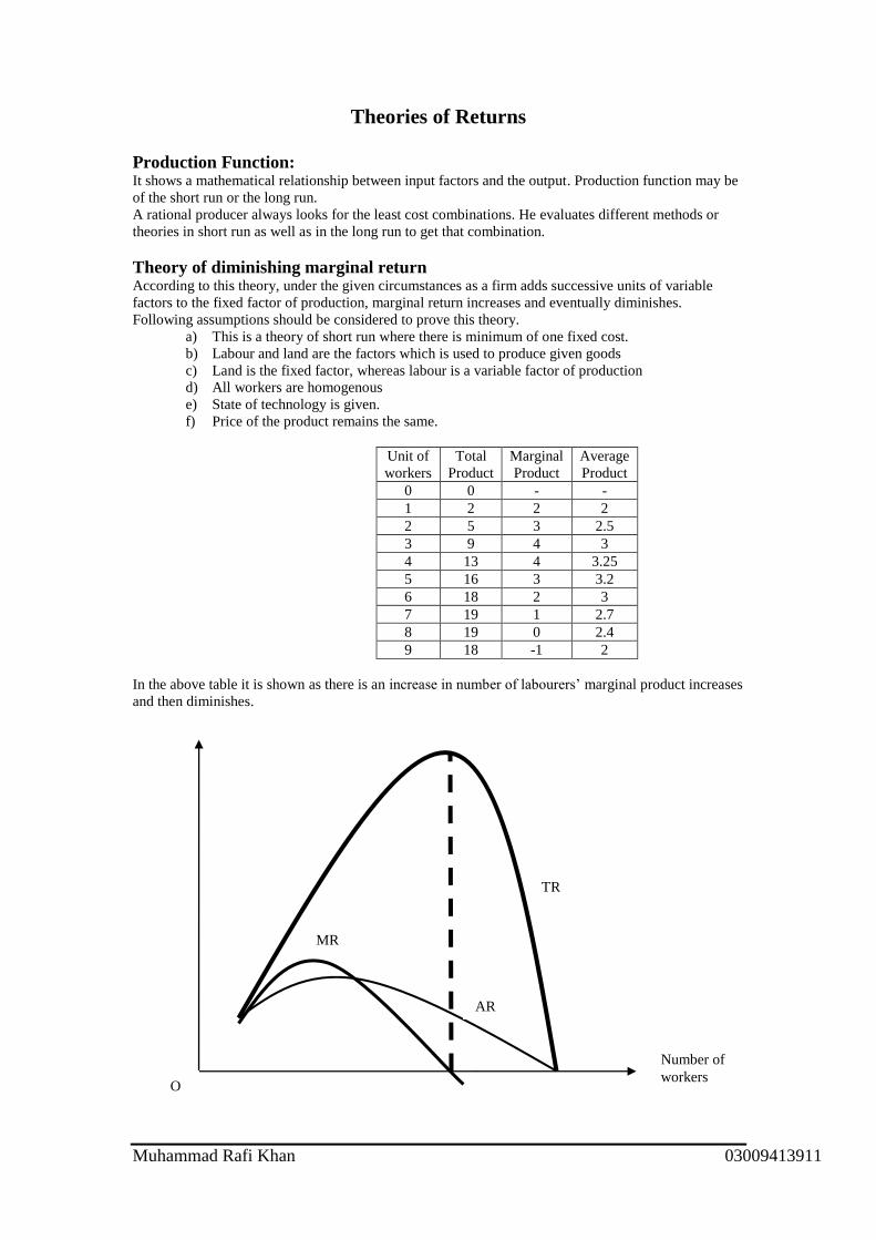
Limitations of the Theory
This is a theory of short run but firms usually take long run decisions,
Return to scale
It is a concept of the long run. In this case firm changes its size of production. For example, if firm
changes its size of production and output is changed at greater proportion, it will be considered,
increasing return to scale. If output changes at the same proportion, it is called as constant return to
scale. However if output changes but at lesser proportion, it is called decreasing returns to scale.
MP3
MP2
MP1
AP2
AP3
AP1
Return to scale
Out put

Muhammad Rafi Khan 03009413911
Since a long run consist on many short runs, therefore a period of return to scale also consist on many
periods of diminishing returns as is shown in the above fig.
Production and time period
Very Short run or momentary time period
In this time period a firm is unable to change its output because all input factors are fixed. In
momentary time period supply is perfectly inelastic and is called as fixed elastic.
Short run
In the short run a firm may change its output by bringing changes in some of its variable
factors of production. However, minimum of one of the factor remain fixed.
Long run
In the long run firm increases its output by changing its size of production. In this time period
all factors of production are varied. Long run is nothing in itself; it is made up of many short runs.
Very long run
In very long run there are some technological changes. In this time period there is a change in
pattern of production. For example, from manual work to mechanization or automation.
Fixed factors of production These factors remain the same in a production process in the given period of time. For
example, in the above case land is the fixed factor of production.
Variable factors of production These factors vary in a production process usually in the same direction with the output over a
period of time. For example, in the above illustration labour is an example of variable factor of
production.
Iso Quant and Iso Cost Curves Iso quant curve shows certain level of output even by employing different combinations of given input
factors. To draw iso quant curve, it is assumed that there are just two factors of production i.e., capital
and labour, and these factors are producing the certain output, e.g., 100 units of the given commodity.
Iso quant map consist on many Iso quant curves, which shows different level of output. As it shifts
outwards, it shows better level of production, and if it shifts leftwards, it shows relatively low level of
output. Iso quant curves are negatively sloped as increase in one factor of production will decrease
another factor, backwards bending due to marginal rate of technical substitution and non-intersecting
because each iso quant curve shows certain level of output but as they intersect, level of output will be
the same which is not possible.
Marginal rate of substitution means the rate at which one factor has to be decreased in order to retain
the same level of productivity if another factor is increased. The marginal rate of technical substitution
shows the tradeoffs between factors, such as capital and labor, that a firm must make in order to keep
output constant. The marginal rate of technical substitution diminishes means that lesser units of one
factor has to forgo to employ an additional unit of another factor.

Muhammad Rafi Khan 03009413911
Iso cost curve shows, different combinations of given input factors which can be purchased by a firm
under given conditions i.e., budget is given, input factors are given, no change in their prices and firm
will have to spend all of its budget. Iso cost curve may be shifted if there is a change in the budget or
prices of input factors. Iso cost curve may be shifted completely, or there is a pivotal or intersecting
shift.
A firm gains least cost combination at that point where Iso cost curve making tangent to the Iso quant
curve.
Labour
Capital
Iso Cost
Iq1 Iq2
Iq3
O
Labour
Capital

Muhammad Rafi Khan 03009413911
Short run Cost and cost curves
Short run Total cost These are expenditures which incur by a firm to produce a given level of output. For instance,
if a firm incurs expenditures of $100 to produce 10 units, it will be considered as total cost of
production.
Short run Fixed cost Fixed costs remain the same in a production process. Such costs do not vary with the output.
This cost is incurred by a firm even at zero output. For example, rent, salaries of managers,
insurance premium, depreciation etc.
Short run Variable cost These costs vary with the output. These costs move in the same direction of output. At zero
level of output, variable cost will be zero. Raw material, fuel charges are common examples
of variable cost.
Total cost (TC) =Total Fixed cost (TFC) +Total variable cost (TVC)
SRTC
TVC
TVC
TC
TFC TVC
TFC
OUTPUT OUTPUT OUTPUT
Iq1 Iq2
Iq3
Labour
O
E
A
B
K1
L1
Capital

Muhammad Rafi Khan 03009413911
The shape of the total variable cost is because of average variable cost which is theoreticallyof „U‟
shaped. In the short run it is because of law of diminishing marginal return.
Average total cost It is the per unit cost of production. It is calculated by dividing total cost of production by
output.
ATC=𝑡𝑜𝑡𝑎𝑙𝑐𝑜𝑠𝑡
𝑡𝑜𝑡𝑎𝑙𝑜𝑢𝑡𝑝𝑢𝑡
Average total cost is of „U-shaped‟ because of diminishing marginal return. When average
product increases, short run average cost falls, and, when average product falls, average cost
rises. When average product is maximum at the certain level of output, average cost will be
minimum.
ATC
Average fixed cost
It is the per unit fixed cost of production. It is calculated by dividing total fixed cost by output.Because
the total fixed cost is, by definition, the same regardless of output, AFC must decline as output
increases. As output rises, the total fixed cost is spread over a larger and larger output.
AFC=𝑡𝑜𝑡𝑎𝑙 𝑓𝑖𝑥𝑒𝑑 𝑐𝑜𝑠𝑡𝑡𝑜𝑡𝑎𝑙𝑜𝑢𝑡𝑝𝑢𝑡
AFC
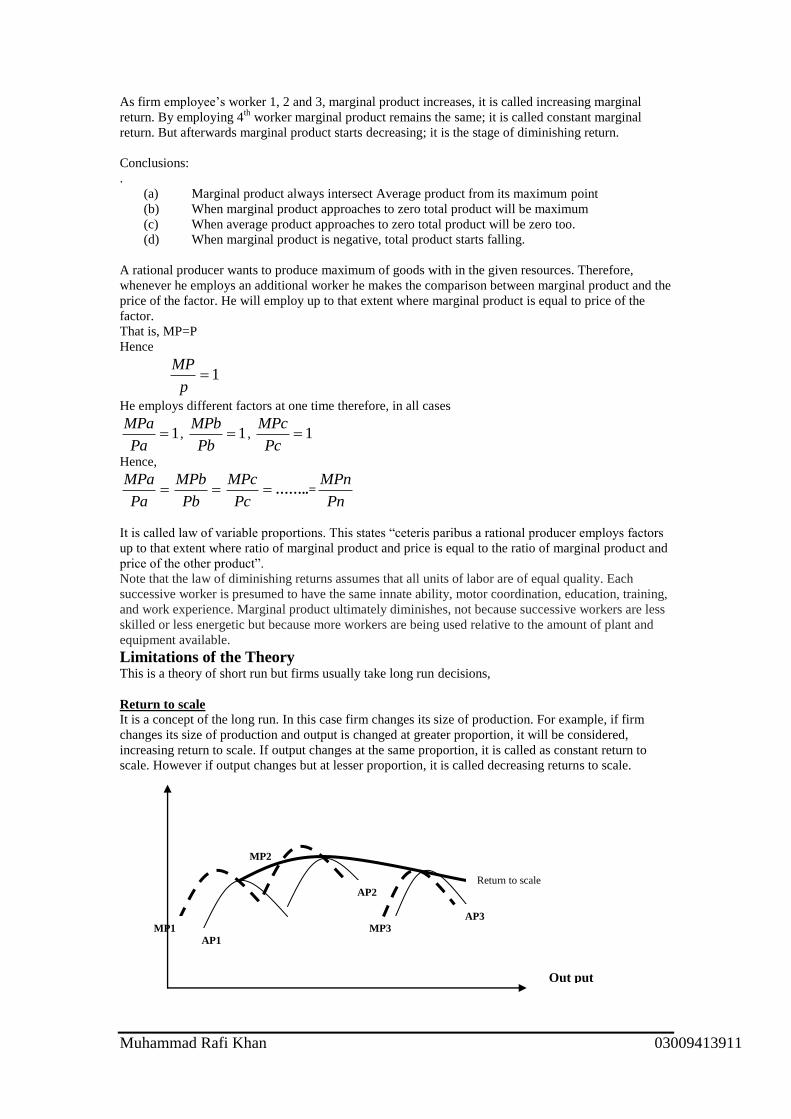
Average variable cost
It is per unit variable cost of production. It is calculated by dividing total variable cost by
output. As added variable resources increase output, AVC declines initially, reaches a
minimum, and then increases again. A graph of AVC is a U-shaped or saucer-shaped curve.
Because total variable cost reflects the law of diminishing returns, so must AVC, which is
derived from total variable cost. Because marginal returns increase initially, fewer and fewer
additional variable resources are needed to produce given units of output. As a result, variable
cost per unit declines. AVC hits the minimum and beyond that point AVC rises asdiminishing
returns require more and more variable resources to produce each additional unit of output.
AFC
Qty
ATC
Qty
Muhammad Rafi Khan 03009413911
AVC=𝑡𝑜𝑡𝑎𝑙 𝑣𝑎𝑟𝑖𝑎𝑏𝑙𝑒 𝑐𝑜𝑠𝑡
𝑡𝑜𝑡𝑎𝑙𝑜𝑢𝑡𝑝𝑢𝑡
AVC
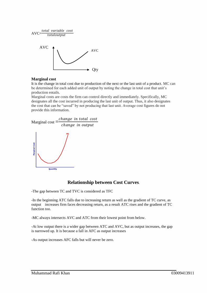
Marginal cost It is the change in total cost due to production of the next or the last unit of a product. MC can
be determined for each added unit of output by noting the change in total cost that unit‟s
production entails.
Marginal costs are costs the firm can control directly and immediately. Specifically, MC
designates all the cost incurred in producing the last unit of output. Thus, it also designates
the cost that can be “saved” by not producing that last unit. Average cost figures do not
provide this information.
Marginal cost =𝑐𝑎𝑛𝑔𝑒 𝑖𝑛 𝑡𝑜𝑡𝑎𝑙 𝑐𝑜𝑠𝑡
𝑐𝑎𝑛𝑔𝑒 𝑖𝑛 𝑜𝑢𝑡𝑝𝑢𝑡
Relationship between Cost Curves.
-The gap between TC and TVC is considered as TFC
-In the beginning ATC falls due to increasing return as well as the gradient of TC curve, as
output increases firm faces decreasing return, as a result ATC rises and the gradient of TC
function too.
-MC always intersects AVC and ATC from their lowest point from below.
-At low output there is a wider gap between ATC and AVC, but as output increases, the gap
is narrowed up. It is because a fall in AFC as output increases
-As output increases AFC falls but will never be zero.
AVC
Qty

Muhammad Rafi Khan 03009413911
Cost and Cost curves in the Long run
A long run is made of with many short runs. In the long run there is no fixed cost,i.e., all costs
are varied. This is why long run total cost emerges from origin.
LRTC
TC
OUTPUT
The shape of the LATC is because of return to scale or because of long run average total cost.
Long Run Average Total Cost (LRATC)
Since long run is made up of with many short run, hence LRATC is also made up of with
many SRATC. LRATC curve is also called as envelope curve, because it envelopes many of short run
average total cost curves. Theoretically it is of „U‟ shaped, because of return to scale. Firstly, firm

Muhammad Rafi Khan 03009413911
experiences increasing return to scale up to point „A‟. From „A‟ to „E‟ having constant return to scale
and beyond „E‟ decreasing return to scale.
Increasing return to scale shows that firm is gaining economies of large scale and decreasing
return to scale shows diseconomies of large scale. The „U‟ shaped LRATC makes tangent
with only one SRATC curve from its lowest point.
However , in some cases LRATC curve may be of saucer shape, it means once firm achieves
least cot combination i.e., lowest possible avg. Cost then can produce at that cost over a
period of time.
LRATC play an important role to achieve main objective of firms i.e. profit maximization.
For instance, in the diagram if the firm produces 130 units, it incurs average cost of about
$2.50 at „B‟, but as it shifts to the next short run or the long run its cost reduces around $2.
It saves half of the $ per unit of production, which will definitely contributes towards profit.
LRATC curve also helps out to determine Minimum Efficient Scale of production. It is the
lowest level of output at which a firm is able to produce at minimum average cost. This is the
point where long run marginal cost curve intersect LRATC from its lowest possible point. It
enables firm to extend range of constant return to scale and also determine to what extends a
firm can produce.
Economies of scale It is reduction in average cost due to increase in the size of the business. At this stage
a firm experiences increasing return to scale. It is a concept of long run because there is a
change in the size of business. A firm gains following economies due to its large size. Such
economies are also called as‟ internal economies‟.
Financial economies relate with the sources of finance. Large firms have more sources
of finance as compare to small firms. For instance, large firms borrow from banks at
favourable terms and conditions, that is, at low rate of interest. Similarly they can raise funds
by issuing shares and debentures at the time of need. This facility is not available to small
firms.
Technical economies relate with the production. Large firms do apply division of labour
and are able to derive advantages of the method. Large firms also prefer to employ skilled
workers, who are more productive, as a result production increases ore then the cost. Large
firms also prefer to use capital intensive method, due to mechanization and automation once
again productivity rises and average cost falls.
Marketing economies relate with buying and selling. Large firms buy raw material in
bulk and get better trade discount. They afford to hire services of specialist buyers, who know
how to buy right good at right price from the right place. Large firms can advertise their
product, which increases turnover. It leads to mass production which saves many costs. Large
firms also appoint specialist sellers who search new markets for producer to sell at favourable
terms and conditions.

Muhammad Rafi Khan 03009413911
Large firms appoint managers who are specialist in respective areas. Such as production
manager, marketing manager, finance manager, etc, as they are specialist, they are more
productive as a result output increases more than the cost of production, hence average cost
falls.
Large firms are more risk bearing as compare to small firms. The ability of large firms
to spread the cost of uncertainty of production over a large level of output and thereby reduce
their unit cost is called as risk bearing economy.
For instance, large firms hold larger stocks and if there is a break down on supply side,
they can continue their production process. Whereas small firms are unable to coop the
situation. Similarly, large firms deal in different lines of products i.e. diversified, hence if
there is a fall in demand for one product then they rely on other products.
Diseconomies of Scale As firm increases its size of production beyond a certain level, its average cost starts rising, it
is called as diseconomies of large scale. At this stage firm experiences decreasing return to
scale.
-Labour diseconomies: In large firms usually division of labour is applied, where workers
may become monotonous due to repetition of task as a result their productivity falls and
average cost of production rises. Secondly there is a possibility of alienation which itself a de-
motivating factor, once again productivity falls.
-Managerial diseconomies: Right decision at right time is the key to success. However, as a
business expands, there are possibilities of lack of communication and co-ordination between
managers. Therefore, managers may not take right decisions at right time and as a result per
unit cost of production rises.
-Increase in supervision cost: as a business expands, firms need to add new lines of
managers and supervisors. Usually it increases cost of production at larger proportion as
compare to output, once again per unit cost of production rises.
-Increase in prices of input factors (external diseconomy): As an industry expands, there is
an increase in demand for input factors, which leads to increase in their prices and as a result
there is an increase in average cost of production. For instance, as industry expands, there is
an increase in demand for skilled worker which causes an increase in the labour cost as well
as there is a shortage of skilled labour, therefore, firms need to employ semi-skilled worker,
who have low productivity but they may have the same wage rate, once again average cost
will rise. Similarly, there will be an increase in rental cost as well due to expansion of the
industry.
Advantages of large scale firms -Economies of large scale
-more profit
-more retained profit
-more sources to spend on research and development leads to better quality, low cost
-high rate of dividend, increase in creditability, easy to raise finance etc.
-in better position to compete in international market
Disadvantages of large scale firms -diseconomies of large scale
-may exploit resources
-destruction of infrastructure
-Consumers „exploitation-low output, high price, excessive profit
-negative externalities etc.

Muhammad Rafi Khan 03009413911
Revenue and Revenue Curves
Total revenue The amount generates by a firm by selling certain units of the given product in specified period of time.
Total Revenue = price × quantity
For example if a firm sells 50 units of a product at the price of £5 each, the total revenue will be £250.
Average Revenue It is the per unit revenue of the given quantity. Price and average revenue are the same.
Average Revenue = 𝑡𝑜𝑡𝑎𝑙 𝑟𝑒𝑣𝑒𝑛𝑢𝑒
𝑡𝑜𝑡𝑎𝑙 𝑜𝑢𝑡𝑝𝑢𝑡
Or
𝑝𝑟𝑖𝑐𝑒 ×𝑞𝑢𝑎𝑛𝑡𝑖𝑡𝑦
𝑞𝑢𝑎𝑛𝑡𝑖𝑡𝑦= price
AR curve is considered as a price line or demand curve.
Marginal Revenue It‟s the change intotal revenue by selling an additional unit of the given product.
MR =𝑐𝑎𝑛𝑔𝑒 𝑖𝑛 𝑡𝑜𝑡𝑎𝑙 𝑟𝑒𝑣𝑒𝑛𝑢𝑒
𝑐𝑎𝑛𝑔𝑒 𝑖𝑛 𝑜𝑢𝑡𝑝𝑢𝑡
For example if a firm generates $50 by selling 10 units and $54 by selling 11 units then the marginal
revenue of selling the 11th
unit is $4.
Revenue curves under perfect competition
In perfect competition all firms are price taker, hence are unable to change prices and sell any quantity
at the given price. This is why, AR and MR remain the same.
Units Price Total Revenue Marginal Revenue Average Revenue
0 $5 - - -
1 $5 $5 $5 $5
2 $5 $10 $5 $5
3 $5 $15 $5 $5
4 $5 $20 $5 $5
5 $5 $25 $5 $5
TR
AR=MR
Qty
Revenue curves under imperfect competition In imperfect competition firms are price maker, therefore to sell more quantity they have to
reduce their prices. This is why demand curve (AR) is negatively sloped and marginal

Muhammad Rafi Khan 03009413911
revenue (MR) curve lies beneath the demand curve. In fact change in MR is always double
than the change in AR, hence, MR‟s x-intercept is half of the x-intercept of AR curve.
Imperfect competition includes monopolies, oligopolies, monopolistic competition etc.
Qty
(units)
Price
($)
TR
($)
MR
($)
AR
($)
0 10 0 - -
1 9 9 9 9
2 8 16 7 8
3 7 21 5 7
4 6 24 3 6
5 5 25 1 5
6 4 24 -1 4
7 3 21 -3 3
8 2 16 -5 2
9 1 9 -7 1
Relationship between AR, MR and TR curves
- MR curve lies beneath the AR curve
- Change in MR is always double as compare to change in AR
- If MR is „+ive’, TR will rise
- If MR=0, TR will be maximum
- If MR is „–ive’, TR will fall
- If MR is „+ive’, then demand will be elastic during that level of output
- Demand will be unitary elastic as MR approaches to zero and at that point TR will be
maximum and also that will be the midpoint of the demand curve (AR).
- If MR is „-ive‟, demand will be price inelastic.
Profit It is the difference between total revenue and total cost. It is positive if total revenue exceeds total cost
and negative if total cost exceeds total revenue. A firm considers loss under this condition. If total
revenue is equal to the total cost at the given level of output, it is called as break-even point for the
firm, i.e., no profit, no loss.

Muhammad Rafi Khan 03009413911
Profit = TR – TC
As output changes profit may be changed, for instance, as output increases total revenue will be
increased as well as total cost. If increase in total revenue is more than the increase in total cost, firm‟s
profit will be increased and, if, total cost exceeds ore then the total revenue, firm incurs loss. Similarly,
as a firm reduces its output, total revenue and total cost fall. If total revenue falls more than the total
cost, firm incurs the loss. However, if total cost falls more than the total revenue, profit will be
increased. As output changes, there may be no change in fixed cost. It also affects the size of the profit.
To increase revenue, a firm should consider price elasticity of demand for its product. For instance if
demand is elastic then by decreasing price more revenue can be generated but if demand is price
inelastic then firm increases price to raise more revenue.
Firms may increase revenue or to reduce average cost through inventions and innovations. As a new
product is introduced effectively through promotion will generate revenue for the firm. Similarly, better
techniques of production will reduce average cost but also quality of products.
Another way to raise revenue is diversification. It is opposite to specialization where a firm increases
lines of products and/or increases branches or number of departments. It helps the firm to spread the
risk as well as increase in revenue.
Another option which a firmhas is competition or collusion. Competition may be on price basis or a
non price competition. Mostly firms reduce prices to increase revenue provided that their demand is
elastic, but in certain cases firms increase prices and create quality consciousness and increase revenue.
It is called as price skimming. Incase of non price competition a firm advertises or uses promotion to
increase its revenue.
In collusion, firms avoid competition to save advertising and promotion costs. On the other hand they
collectively determine the price which maximizes industry‟ profit, it may rise profit of the most of the
firms.
In the short run, since fixed cost remains the same hence as output increases, average fixed cost will
fall, however, if firm should make policies to reduce average variable cost like increase productivity of
workers or use better techniques of production.
A firm can reduce its average cost of production by increasing its size of production i.e. economies of
large scale. For instance, technical economies, financial economies, marketing economies, managerial
economies, risk bearing economies etc. may help out a firm to reduce its average cost of production.
Accountant profit vs Economist profit According to accountant profit only explicit costs are included, like labour cost, rental cost, capital cost
etc. whereas in case of economist profit implicit costs are also considered. An example of an implicit
cost is the opportunity cost of a sole proprietor working in her own business. If she works somewhere
else, she can earn certain income which is forgone now. Therefore, to calculate economist profit that
income must be deducted from the accountant‟ profit.
Accountant‟s profit = Total Revenue – Total Cost
Economist‟s profit = Accountant‟s profit – opportunity cost
Objectives of a firm
Profit maximization Traditionally it is the main objective of a firm. According to this a firm prefers to produce at that point
where it can make maximum of profit. To gain that level of production a firm may follow to different
rules i.e. total revenue, total cost rule and marginal cost marginal revenue rule. According to the total
revenue and total cost method a firm produces to that extent where there is a maximum difference
between total revenue and total cost.
According to marginal cost and marginal revenue rule, a firm produces to that extent where marginal
revenue and marginal cost are equal. Before the equilibrium output MR is more than the MC and a
firm which wants to maximize its profit wants to earn every profit on each and every unit. It wants to
earn maximum profit on the whole.

Muhammad Rafi Khan 03009413911
However, in practice it is not possible for a firm to make maximum of the profit in the long
run due to following reasons.
Firstly, firms do not make maximum profit because it may attract new firms, hence competition will be
increased. Secondly, firms are reluctant to make maximum profit to avoid government watch dogs.
Thirdly, it may damage the relationship between stakeholders, such as consumers and workers.
Fourthly, it may be possible to the certain scale of production, but it is difficult to calculate MR and
MC in mass production. Usually firms work out on their average cost and add on a profit margin to
determine the selling price. In some cases management may have some other objectives. It is also not
possible, where goods are not divisible by nature. Profit maximization is also not possible in service
sector.
Managerial and Behavioural Theories
Sales Revenue Maximization A firm can maximize its sales revenue by producing up to that extent where MR approaches to
zero. A firm is prepared to charge low prices when it wants to increase its market share. This is a price
penetration policy. A firm can make abnormal profit if TR is more than TC at the given output. This
policy is also chosen when management salaries are linked with the sales. The solution of this conflict
of interest is to offer management some shares as a bonus or link their salaries to profit. This policy is
also formed by the state when industry experiences growth and a firm want to increase its market share.
D=AR=M
R
P
O Quantity
MC
AR
MR
QUANTITY
E
O Q

Muhammad Rafi Khan 03009413911
Sales Maximization This policy maximizes sales instead of sales revenue maximization. Theoretically it is possible
when a firm produces to that extent where average revenue approaches to zero. In practice a firm may
produce up to the breakeven point, where total revenue is equal to the total cost. A higher output
implies loss making behaviour. It is possible when a firm may subsidize its loss by using the profit of
some other firms. It could be positive in state-owned business organization which has some social
objectives. Another possibility may be a firm wants to clear its existing stock at the end of a season or
due to an exit from the market, so, to make any recovery.
Satisficing Profit. According to this policy a firm is determined to make reasonable profit, sufficient to keep on
its activities or to satisfy its share holders. It may wants to keep all stakeholders happy. It may spend
more on wages or on the improvement of working conditions, which increases cost of production. It
may charge low prices to keep its customers happy. This profit may be anywhere between normal
profit and positive economic profit.
Survival Mainly it will be the objective of a firm when there is question mark on its existence and the firm finds
it difficult to survive. Usually it happens at the early stage of the firm, when existing firms make it
difficult to penetrate. Secondly, when trading becomes difficult due to fall in demand for the product or
due to bad debts or losing confidence of customer. Thirdly, when there is downturn of the economy
and presences of recessionary pressure make it difficult for the firm to survive. Under such condition(s)
primary objective is the survival.
Conclusion: The ultimate objective of all business organization is profit maximization. All other
objective are formed for the short run by forgoing objective of profit maximization.
Types of profit
Normal profit It is the minimum profit which is required to a firm to keep its existence in the long run. At equilibrium
output i.e. (where marginal revenue is equal to marginal cost), average revenue is equal to the average
cost. At this level of profit „economic profit‟ is zero.

Muhammad Rafi Khan 03009413911
Perfect competition Imperfect competition
This will be the break- even point for the firm because at this level of output total revenue is equal to
the total cost. Usually it is thought that there is no profit for the entrepreneur but actually it takes profit
as a reward of a factor of production which is measured as explicit cost.
Abnormal Profit
It is the any profit which in excess of the normal profit. At equilibrium output average
revenue exceed average total cost. At this point a firm makes positive economic
profit.
Perfect competition Imperfect competition
Loss/ Subnormal profit with contribution
A firm incurs loss if at the equilibrium output its average total cost exceeds its
average revenue. At this point economic profit of the firm will be negative. However,
it will continue its production unless it meets to its average variable cost. As is shown
in the following figures, where average total cost is passing above the average
revenue curve and shaded area show the amount of loss at output OQ.
Muhammad Rafi Khan 03009413911
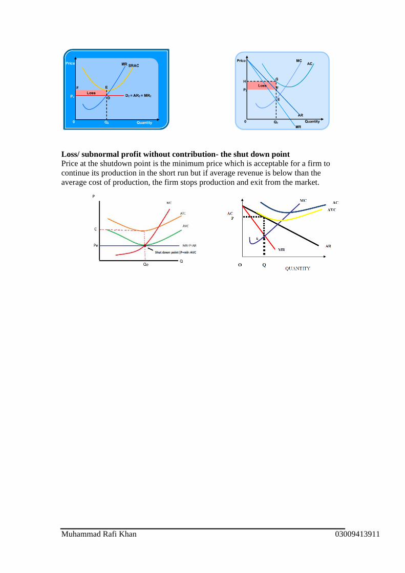
Loss/ subnormal profit without contribution- the shut down point
Price at the shutdown point is the minimum price which is acceptable for a firm to
continue its production in the short run but if average revenue is below than the
average cost of production, the firm stops production and exit from the market.