Hitotsubashi University Repository

Title Theories of Exchange Rates Determination : A Review

Author(s) Ogawa, Eiji

CitationHitotsubashi journal of commerce and management,

22(1): 27-54

Issue Date 1987-12

Type Departmental Bulletin Paper

Text Version publisher

URL http://doi.org/10.15057/6165

Right

Hitotsubashi Journal of Commerce and Management 22 (1987) pp. 27-54. C The Hitotsubashi Academy

THEORIES OF EXCHANGE RATES DETERMlNATION = A REVIEW

EIJI OGAWA

I . Introduction

Theories of exchange rates determination have changed since the exchange rate system

shifted to the floating rates system. Traditional theories, developed during the period of

fixed exchange rates, including the elasticity approach and the absorption approach, focused

mainly on the real sector. However, especially in the current period of floating exchange

rates, the monetary sector is another important element determining exchange rates. I

review recent developments in the theories of exchange rates determination in this paper.

I emphasize that asset markets are important in determining exchange rates. Moreover. I

pay special attention to the interaction between asset markets and the current account, and

to the interaction between stocks, flows, and stock adjustments.

In Sections 2 and 3, I consider the two traditional theories: the elasticity approach and

the absorption approach. These theories were initially concerned with the effects of de-

valuation on the trade balance. Here I apply them to exchange rate determination. The

elasticity approach focuses on the domestic goods market and the foreign goods market,

while the absorption approach focuses on the expenditures of economy as a whole. How-

ever, neither approach models the monetary sector explicitly.

In Section 4, I consider the Mundell-Fleming model, where the exchange rate is deter-

mined by interactions between the real sector and the monetary sector. In contrast to the

traditional approaches which focused only on flows, this model also considers stocks.

In Section 5, I consider the asset market approach. Models which belong to this cat-

egory share an emphasis on the role of expectations in determining asset market equilibrium,

although they differ in terms of the roles played by money and other assets.

I consider the monetary approach as the basic model of the asset market approach.

An essential element in the monetary model is purchasing power parity. However, we know from the recent experiences that purchasing power parity does not hold at least in the

short-run. Two related models which relax the ppp assumption include the overshooting

model and the portfolio-balance approach. The overshooting model assumes rigid prices

and perfect substitutability between domestic and foreign bonds. On the other hand, the

portfolio-balance approach assumes imperfect substitutability between domestic and foreign

bonds.

* This paper was written during the author's visit to Harvard University. I would like to thank Professor

Jeff Sachs for permitting me to quote his simulation study in this paper. Also, I would like to thank Professor Toshiya Hanawa, Professor Jeff Sachs, and Andrew Warner for their helpfu] advice and editing the Engl i sh .

28 HrroTSUBASHI JOURNAL OF COMMERCE AND MANAGEMENT [December

In Section 6, I consider models developed to emphasize the interaction between asset

markets and the current account. These models consider the current account in connec-

tion to asset stock adjustments in a dynamic setting. Modelling the dynamic adjustments

through the current account makes it possible to explain the deviation of actual exchange

rates from ppp in the adjustment processes even though ppp holds in the steady state.

In Section 7, I apply the asset market approach to explain theoretically the dollar ap-

preciation in the early 1980s. I emphasize the U.S. budget deficits as a main cause of the

dollar appreciation. And then I review an application of a simulation model to explain

the dollar appreciation done by Sachs & Roubini. Their result is that the dollar apprecia-

tion and the U.S, and Japanese trade imbalances are mainly caused by the differential fiscal

policy stances of the U,S, and Japan.

In Section 8, I consider the pass-through effects of exchange rates on domestic prices.

II. Elasticity Approach

Now consider how the elasticity approach can explain the determination of exchange rates under the fiexible exchange rate system. In order to stress the role of the goods market

rather than that of the asset market, assume a state without any international capital flows.

Consider two countries : one domestic and one foreign. Assume that the domestic country and the foreign country specialize in the production of goods I and 2 respectively.

Both goods are traded. For simplicity, assume there are no non-tradable goods.

(1) P1=EPl* (2) P2=EP2*

(3) IM=1M(P2) +(r

(4) X=X(P1)+p (5) IM*=1M*(Pl*)+a' (6) X*=X*(p2*)+p*

(7) X=1M* (8) X*=1M (9) B=PIX-P21M=-EB*=0

where Pl=the domestic price of good l, Pl*=the foreign price of good l, P2=the domestic

price of good 2, P2*=the foreign price of good 2. E=the exchange rate (the relative price

of domestic currency in terms of foreign currency), IM=the domestic import demand for

good 2, X=the domestic export supply of good 1, IM*=the foreign import demand for

good 1, X*=the foreign export supply of good 2, a=a shift parameter for domestic import

demand, p=a shift parameter for domestic export supply, a*=a shift parameter for foreign

import demand, p*=a shift parameter for foreign export supply.

Eqs. (1) and (2) represent the law of one price. Eqs. (3)-(6) are the demand and supply

functions for each good. For simplicity, assume that all of the cross elasticities are zero.

Eqs. (7) and (8) are market clearing conditions. Eq. (9) assumes balance in the trade ac-

counts of both countries.

An equilibrium exchange rate can be derived from the above system of equations.

1987] THEORIES OF EXCHANGE RATES DETERMINATION : A REVIEW 29

(10) E=E(a, ~, a*, p*)

Thus, the equilibrium exchange rate depends on the shift parameters of import demand

and export supply in both countries. Furthermore, the effect on the exchange rate of a

change in one of the shift parameters depends on each elasticity. For example, an effect of

a change in domestic import demand on the exchange rate is derived:

(~ * - e)(v + I ) da dE (1 l) = E ee*(~+v*+1)-~~*(e+5*+ 1) M

where e, e*, ~, and ~* are the price elasticities of deand for good 2, demand for good l, sup-

ply of good 1, and supply of good 2, respectively.

The numerator in eq. (11) is unambiguously positive. However, the sign of the de-

nominator is ambiguous. Exchange rate stability requires that the sign of the denominator

be positive in a state without any capital flows. This constraint is called the Bickerdike

condition. The Marshall-Lerner condition is sufiicient for the Bickerdike condition (What-

ever the supply elasticities may be, if the absolute demand elasticities sum to at least l, the

Bickerdike condition holds,)

III. Absorption Approach

Now consider how the absorption approach can explain the determination of exchange

rates under a flexible exchange rate system. Use a two country formulation along the lines

of Harberger's (1950) model. Both the domestic and foreign countries are assumed to spec-

ialize in production. Moreover, for simplicity, assume that there are no international

capital flows. This is a short-run analysis in the sense that domestic prices are fixed, with

each country supplying any desired amount of output at the given prices, normalized at unity.

(12) Y=A + X- EIM

(13) Y*=A*+X*-IM*/E (14) A=A(Y,E)+a (15) IM=1M(Y. E)+b (16) A*=A*(Y*. E)+a*

(17) IM*=1M*(Y*.E)+b*

(18) X-EIM=X*-IM*/E=0 where Y=income, A=absorption, a=a shift parameter for home absorption, b=a shift parameter for home import demand, a*=a shift parameter for foreign absorption, b*=a shift parameter for foreign import demand.

Eqs. (12) and (13) represent equilibrium in the home goods market and in the foreign

goods market respectively. Eqs. (14)-(17) represent the absorption and the import func-

tions in each country. Eq. (18) represents balance in the trade account in the absence of

capital flows.

Eqs. (12)-(18) determine a reduced form equilibrium exchange rate:

(19) E=E(Y, Y*,. a, b, a*, b*)

30 HITOTSUBASHI JOURNAL OF COMMERCE AND MANAGEMENT [December

The determination of the exchange rate depends on the absorption and the import demand

in both countries.

This model can be used to consider how a change in absorption or import demand affects the exchange rate in a case with repercussion effects. In a stable state, the partial

differential coefficients of the shift parameters of home absorption and home import demand

in eq. (19) are positive. As for foreign absorption and foreign import demand, their partial

coefficients are negative.

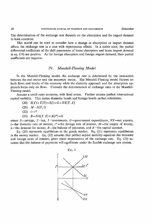
IV. Mundell-Fleming Model

In the Mundell-Fleming model, the exchange rate is determined by the interaction

between the real sector and the monetary sector. The Mundell-Fleming model focuses on

both flows and stocks of the economy while the elasticity approach and the absorption ap-

proach focus only on fiows. Consider the determination of exchange rates in the Mundell-

Fleming model. Assume a small open economy, with fixed prices. Further assume perfect international

capital mobility. This makes domestic bonds and foreign bonds perfect substitutes.

(20) S(Y)+T(Y)=1(i)+G+NX(Y. E) (21) M=L(Y, i)

(22) i=i*

(23) B=NX(Y, E)+K(i*)=0 where S=savings. T=tax, I=investments, G=government expenditures, NX=net exports, i=the domestic rate of interest, i*=the foreign rate of interest, M=the supply of money,

L=the demand for money, B=the balance of payments, and K=the capital account. Eq. (20) represents equilibrium in the goods market. Eq. (21) represents equilibrium

in the money market. Eq. (22) assumes that perfect capital mobility equalizes the domestic

and foreign rates of interest, given static expectations of the exchange rate. Eq. (23) as-

sumes that the balance of payments will equilibrate under the flexible exchange rate system.

FIG. 1

L〃

戸 6ヨ戸

1111111一一

1S

1－1

ア

1，，

1■一一

1　　■　　一　一　　’　　一　　一一　　■　一一　■

FFE XX

Y

1987] THEORJES OF EXCHANCE RATES DETERMINATION

FIG. 2

工〃’

＼ ＿／五〃’

＼ ■　／ρ月

1＝戸l　l

■1∫1＼■1：ム旭’l11s　l　r1　■1　■■■　■

■　1■　　11　■

ll一’’一1■■一■一’　　1＼、9’■　　＼l　FF一一一’一1－11’■■ア、↓〃・

亙 xx

r~¥

~¥

A REVIEW

FIG. 3

LM ¥P Q ' i= i*

¥ ¥IS'

ISY

31

¥r~~:R'

-----'- - : '¥ ___________., ¥ '¥FF' ~ Q IFF

¥f XX'

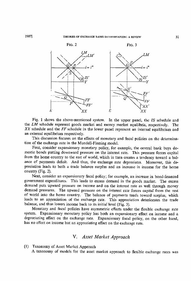
Fig. I shows the above-mentioned system. In the upper panel, the IS schedule and the LM schedule represent goods market and money market equilibria, respectively. The

XX schedule and the FF schedule in the lower panel represent an internal equilibrium and

an external equilibrium respectively.

This discussion focuses on the effects of monetary and fiscal policies on the determina-

tion of the exchange rate in the Mundell-Fleming model.

First, consider expansionary monetary policy, for example, the central bank buys do-

mestic bonds putting downward pressure on the interest rate. This pressure forces capital

from the home country to the rest of world, which in turn creates a tendency toward a bal-

ance of payments deficit. And thus, the exchange rate depreciates. Moreover, this de-

preciation leads to both a trade balance surplus and an increase in income for the home

country (Fig. 2).

Next, consider an expansionary fiscal policy ; for example, an increase in bond-financed

government expenditures. This leads to excess demand in the goods market. The excess demand puts upward pressure on income and on the interest rate as well through money demand pressures. The upward pressure on the interest rate forces capital from the rest

of world into the home country. The balance of payments tends toward surplus, which

leads to an appreciation of the exchange rate. This appreciation deteriorates the trade

balance, and thus lowers income back to its initial level (Fig. 3).

Monetary and fiscal policies have asymmetric effects under the fiexible exchange rate

system. Expansionary monetary policy has both an expansionary effect on income and a depreciating effect on the exchange rate. Expansionary fiscal policy, on the other hand,

has no effect on income but an appreciating effect on the exchange rate.

V. Asset Market Approach

(1) Taxonomy of Asset Market Approach A taxonomy of models for the asset market approach to flexible exchange rates was

32 HITOTSUBASHI JOURNAL OF COMMERCE AND MANACEMENT [December

proposed by Frankel (1983). The most important dichotomy is whether or not domestic and foreign bonds are assumed to be perfect substitutes in the asset-holders' portfolios.

The assumption o.f perfect substitutability implies that asset holders are indifferent regard-

ing the composition of their bond portfolios as long ~s the expected rates of return on the

two countries' bonds are the same. Given this assumption, uncov~red interest parity holds.

Models in which domestic and foreign bonds are assumed to be perfect substitutes

belong to the monetary approach. Given that uncovered interest parity holds, bond sup-

plies become irrelevent. The responsibility for determining the exchange rate is shifted

onto the money market. Models in which foreign and domestic bonds are assumed to be imperfect substitutes

belong to the portfolio-balance approach. In this approach asset holders wish to allocate

their portfolios in shares that are well-defined functions of expected rates of return.

Models engendered by the monetary approach are further subdivided by whether prices

are flexible or sticky. The monetarist model assumes perfect price flexibility. Given this

assumption, purchasing power parity must hold in both the long-run and the short-run.

The overshooting model assumes the sticky prices. In this model overshooting of the ex-

change rate is explained by assuming that the adjustment speed of goods prices is slower

than that of assets price. Purchasing power parity holds only in the long-run.

Models engendered by the portfolio-balance approach are classified into the uniform

preference model, the small country model, and the preferred local habit model according

to Frankel (1983). Frankel's criterion is based on the structure of asset holders' portfolio

preferences. Alternatively, Fukao (1983) classified them into the inilation risk model, the

real exchange rate risk model, and other models according to the role of risk.

(2) Monetarist Model The monetraist model consists of equations defined by money market equilibrium,

purchasing power parity, and uncovered interest parity.

(24) m~P+cy-1i (25) m*~P*+cy*-1i* (26) e~P-P* (27) i-i*=~'

where ~'=the expected rate of depreciation: Any lower-case variable (except for the interest

rate) is the logarithm of the corresponding upper-case variable.

Assume that expectations are rational and the system is stable. For simplicity, assume

that income growth is exogeneous and equal to zero. From the equation for purchasing power parity, it can be shown that the expected rate of depreciation is equal to the current

relative monetary growth rate (p-p*). The exchange rate is determined according to the

following equation:

(28) e=(m-m*)-c(y-y*)+1(p-p*) The determination of the exchange rate in the monetarist model is based on the purchasing

power parity equation. Therefore, the monetarist model requires that ppp always holds.

As such, the assumption of perfectly flexible prices is essential to the monetarist model.

(3) Overshooting Model

1987] THEORIES OF EXCHANGE RATES DETERMINATION : A REVIEW 33

The overshooting model consists of the money market equilibrium equation (24), the

uncovered intreest parity equation (27), and the dynamic adjustment of the goods market

equation (30). However, the ppp equation (26) holds only in the long-run. Assume that individuals have perfect foresight in their expectations of the exchange rate.

(24) m~P+cy-),i (26a) ~=p-p*

(27) i-i*=~'

(29) ~'=e

(30) p=v[u+6(e-p)-(Ti+ry+~y*-y]

where e=the actual rate of depreciation, p.=the rate of inflation, u=a shift parameter for

goods demand or supply. Bars over variables represent long-run equilibrium levels.

Two dynamic adjustment equations are derived from the system in terms of deviation

from long-run equilibrium levels.

(31) ~=(p-p)/1

(32) p=,J[6(e-~)+(a +a/A)(p-p)]

Using eqs. (31) and (32), schedules for ~=0 and p=0 are drawn in Fig. 4. A dynam-

ically stable system requires that the economy must always stay on a saddle path (shown

as the AA schedule in Fig. 4). For example, suppose there is an expansion of the money

supply in the home country (Fig. 5). Then the new long-run equilibrium is the point E2'

In the adjustment process, the economy immediately jumps from the initial equilibrium

point Eo to the point E1 on the AA schedule (notice the overshooting). Therefore, the

economy moves to the new long-run equilibrium point along the AA schedule. Thus, the overshooting in this model is attributed to the stickiness of goods prices.

Next, using the above-mentioned two country model, the exchange rate determination

equation in the overshooting model can be derived. As for expectations of the exchange

rate, assume that in the short-run, when the exchange rate deviates from its equilibrium

path, it is expected to close that gap with a speed of adjustment e; while in the long-run,

when the exchange rate lies on its equilibrium path, it is expected to increase at the expected

rate of relative inflation p-p* :

FIG. 4

e=0

e e

34 HrrOTSUBASHI JOURNAL OF COMMERCE AND MANAGEMENT

FIG. 5

[December

p= O'

l-/ t p=0 e=0

e= O

eo el

(29a) ~"= -O(e-~)+p-p*

Eqs. (24), (25), (26a), (27), and (29a) determine the exchange rate equation :

(33) e=(m-m*)-ip(y-y*)+1(p-p*)-(1/6)[(i-F!)-(i*-p*)]

.Eq. (33) is identical to the monetarist equation (28) except for the addition of a fourth ex-

~'planatory variable, the real interest differential. In this model, a deviation of the actual

exchange rate from ppp in the short-run is explained by a real interest differential.

(4) Portfolio-balance Approach In the portfolio-balance approach, domestic and foreign bonds are assumed to be im-

perfect substitutes. There are many reasons why two assets can be imperfect substitutes.

This section focuses on the exchange risk,

Assume domestic and foreign bonds differ in only one aspect : their currency of de-

nomination. Investors, in order to diversify the risk that comes from exchange rate var-

iability, balance their bond portfolios between domestic and foreign bonds in proportions

that depend on the expected relative rates of return on risk premia.

Assume that all active participants in the market have the same portfolio preferences.

Then it is possible to add up individual asset demand functions into an aggregate asset

demand equation (34):

(34) B/EF=p(i-i*-e.)

where B=the stock of domestic-denominated bonds, F=the stock of foreign-denominated bonds, p=a positive-valued function representing portfolio preferences.

The simplest portfolio-balance model specifies static expectations; ~'=0. Then the exchange rate is simply determined by relative bond supplies and the interest differential :

(35) e=-a-p(i-i*)+b-f where b s logB, f s logF.

It is obvious from eq. (35) that the stocks of domestic and foreign bonds are important

in determining the exchange rate in the portfolio-balance approach. Since flows of foreign

assets are reflected in the current accQuJrt, it is n~cess~ry tq consider the interaction between

the assets market and the current account.

1987] THEORIES OF EXCHANGE RATES DETERMINATION : A REVIEW 35

VI. Asset Market Approach and the Current Account

This section discusses the models which introduced the interaction between the assets

market and the current account into the asset market approach. In particular, consider

the Kouri model, the Dornbusch-Fischer model, and the Branson model.

(1) Kouri Model Kouri (1976) used a dynamic model to show that the exchange rate is determined by

monetary assets market equilibrium and short-run expectations. In the Kouri model, the

time path from the monetary short-run equilibrium to the long-run equilibrium is deter-

mined by a process of asset accumulation through the current account.

The Kouri model assumes a small open economy. It is further assumed that the assets

in the economy consist of home currency and foreign currency. The economy produces only traded goods and their relative prices are fixed in the world market.

(36) F=CA=Y-C(Y-T. W)-G (37) W=M/P+F (38) M/P=L(i', Y. W)

(39) F=F(~', Y, W)

(40) P=E where F=the capital flow, CA =the current account, W=the stock of monetary assets.

The assets market equilibrium equation (41) and the capital flow=current account equation (42) can be derived in the following reduced forms.

(41) E=A(F,Y, M, e')

(42) F=CA(E;F, Y, M. G. T)

In the short-run, the exchange rate is determined at the level at which the assets market

equilibrates (given the stock variables of domestic money and foreign assets (eq. (41)). The

exchange rate determined in the assets market does not always equilibrate the current ac-

count. Eq. (42) shows a process of asset accumulation through the current account.

Fig. 6 demonstrates the characteristics of this model. The assets market equilibrium

FIG. 6

一γ

Eλ

．BEo’一一■．■一一一

んB］

■一．一Ir1■一一一■一‘一　1

＆．、．．．．．1．．λ、

■

11■

1■

B ■11

一11

’■ll一，1■■111I1■1■ll

1　－IlI　1

」

γ 〃1 li●η一D F∩F。

ム

F=B Fo Fl F

36 ~lITOTSUBASHI JOURNAL OF COMMERCE AND MANAGEMENT [Decerhber

equation (41) is shown as the AA schedule in the right panel. The exchange rate is deter-

mined, given the stock of foreign assets at each point in time. The capital fiow=current

account equation (42) is shown as the BB schedule in the left panel. If the current account

is not balanced at the short-run exchange rate, the imbalance increas~s dr decreases the

stock of foreign assets, shifting the BB schedule. Finally, the economy reaches the long-

run equilibrium. ' (2) Dornbusch-Fischer Model ' The Dornbusch-Fischer (1980) model extends the Kouri model by considering dynam-

ically the relationship between the exchan~e rate and the current account. The role of

expectations are explicitly shown in the'model. ' . -The model assumes exported goods and imported goods. The terpls of trade may bc

explicitly shown in this model. Doniestic residents are assumed to hold domestic money

and foreign bonds. Individuals have p'erfect foresight in their expectation of the exchange

rate .

(43) m=k(i*+ee)D,+pf]

(44) y=D(p, w)+X(p)

(45) w~m+pf/i* (46) S=S(w)=pf/i*

(47) ~'=~

where p(~EP*/P)=the terms of trade, D=the domestic demand for the domestic goods,

X=the foreign demand for the domestic good, m~M/P, w~ W/P, f~F/P. Eq. (43) represents money market equilibrium. Eq. (44) represents goods market

equilibrium. Eq. (45) is the definition of real wealth. Eq. (46) implies that the current

account (the current account is equal to savings as there is no government sector nor invest-

ment in this model) is equal to the capital flow. Eq. (47) represents perfect foresight re-

garding the rate of depreciation. The dynamic of the exchange rate and the accumulation of foreign assets can be de-

rived as follows:

(48) ~=T(f, E/(M/P ))

FIG. 7 FIG. 8 E ¥ E'/ J = O'

~' -_------

E ll~~~___ H El ~~~~//H j f=0

~ ----- : ¥ ! ~=0'

: ~=0

7 f' ' ~'~~' f f f

1987]･ THEORIES OF EXCHANGE RATES DETERMINATION : A REVIEW 37

(49) f=ip(f E/(M/P*)) : .･. . Fig. 7 shows the dynamic system generated by eqs.~j48) and (49). In the Fig, 7 the

FF schedule shows the saddle path, along whic~,･the eccnomy converges to the long-run

equilibrium. . . '~_ i This model can show the dynamic effecfs of certain' ~isturbances. For example, the

following case is interesting: suppose it'is ann~unced howj that the nominal money supply

will increase in the future (Fig. 8),･･~Th~ ･d~namic system defined by this model suggests that the current account improves .at fifst. Then as the e;xchange rate begins depreciating,

the current account declines. } ,

(3) Branson Model While the Kouri and Dornbusch-Fischer models allow for only domestic money as a

domestic asset, the Branson (1977) model considers domestic money, domestic bonds, and foreign bonds as assets. After that, Branson (1~84) :extended the model to a rational ex-

pectations framework... . _. . ' ___: ･･~ ' ･'~ ' -The model assumes a small open econom!･'･･ thq assets~vailable, in-thje home country

are aggregated into the domesticjmoney--sl6ck:_ the ,holdjngs of d6mestically issued assets

, and thef~net holdings of foreign-issue4 assets (denom-(denominated in the home currency) _ inated in the foreign currency). ' ' '

(50) M~R+BcFm(i,.i*+e.).W ___ _ _ . ._ , ,_ ･ ____ _. ___ _.. _

(51) Bp=b(i,'i*+~')･W - ･' -~ (52) EFp-~f(i, i~+~')･W ~. ' .:･ -(53) W=M+Bp+EFp , . " ' (54) BC+Bp=B (55) Fp+R=F (56) F=NX(E/P, W, z)+i*F

(57) ~,=~

where R=central bank foreign reserves, Bc=government debt held by central bank, Bp= government debt held by the private sector, Fp=net claims pn foreigners held by the dom-

estic private sector, z=an exogenous shift factor.

Eqs. (50), (51), and (52) represent money, domestic bonds, and foreign bonds market

equilibria conditions, respectively. Eq. (53) is a balance sheet constraint. Eqs. (54) and

(55) allow domestic and foreign bonds to be held by both the private sector and the central

bank. Eq. (56) shows how an accumulation of net foreign assets might occur. Eq. (57) implies perfect foresight regarding the exchange rate.

A dynamic model of the interaction between foreign assets and the exchange rate can

be derived by solving eqs. (50)-(57).

(58) i=ep(EFp/W. M/W)

(59) F=NX(E/P. W, z)+i*F

This system is drawn in Fig. 9. The ~=0 schedule represents a locus along which the

exchange rate does not change. The F=0 schedule represents a locus along which the

38 HrroTSUBASHI JOURNAL OF COMMERCE AND MANAGEMENT

FIG. 9

[December

亙

、＼

‘ 一　・　　・

＼ ●

　　F＼●θ二〇

　　　　　　F1　〃＝亙Fpα〃刎　∂！一；’　ガ　　∂ク

F=0

FP

FP

FIG. 10

FP

E E＼＼ 一　　　　　　　■　　　　　　■

一 一■＼　　・　　F＝O ■F＝

●ε；0

＼●2；O

　　　　Fp〃＞班p0γ噌・芸

　　　　　Fp〃〈EFp07箒・割

"_'_~ l

',

F=0

I., > ~ l I

'"

F= O

FIG. I l

F I]

stock of foreign assets does not change. Equilibrium of the system is shown in Fig. 9.

There is one saddle path into the equilibrium shown by the PP schedule. For a given value

of Fp, it is assumed that following a disturbance, the market will pick the value for e that

puts the system on the saddle path toward equilibrium.

Reaction to exogenous shocks can be observed in this model. In the case of an un-

anticipated expansionary open-market operation, fixed prices would yield ･overshooting of the exchange rate, If the domestic price level immediately reacts by rising by the same

proportion as the money stock, the system would yield overshooting or undershooting,

depending on the initial portfolio distribution and the degree of substitutability among

1987] THEORIES OF EXCHANGE RATES DETERMINATION : A REVIEW

domestic money, domestic bonds, and foreign bonds (Fig, lO). The model shows shooting of the exchange rate in response to unanticipated real disturbances (Fig. 1 1).

39

under-

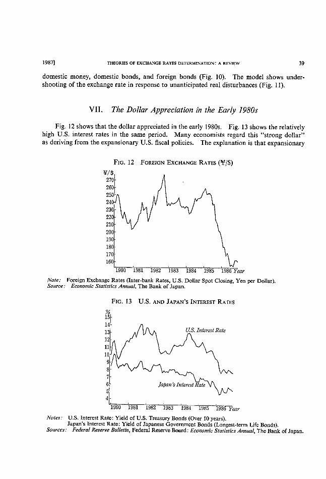
VII. The Dollar Appreciation in the Early 1980s

Fig. 12 shows that the dollar appreciated in the early 1980s. Fig. 13 shows the relatively

high U.S. interest rates in the same period. Many economists regard this "strong dollar"

as deriving from the expansionary U.S. fiscal policies. The explanation is that expansionary

FIG. 12 FoRl~1GN EXCHANGE RATES (~~/$)

~/S 270

260

250

240

230

220

210

200

190

180

170

160

No te :

Source :

1980 1981 1982 1983 1984 1985 1986 Year

Foreign Exchange Rates (Inter-bank Rates, U.S. Dollar Spot Closing, Yen per Dollar). Economic Statistics Annual, The Bank of Japan.

FIG. 1 3 U.S. AND JAPAN'S INTEREST RATES

%

Notes:

Sources :

15

14

13

12

11

10

9 8

6 5 4

U.S. Interest Rate

Japan ~ Interest Rate

1980 1981 1982 1983 1984 1985 1986 Year

U.S. Interest Rate : Yield of U.S. Treasury Bonds (Over 10 years).

Japan's Interest Rate: Yield of Japanese Government Bonds (Longest-term Life Bonds). Federal Reserve Bulletin, Federal Reserve Board : Economic Statistics Annual, The Bank of Japan.

40 HITOTSUBASHI JOURNAL OF COMMERCE AND MANAGEMENT [December

U.S. ,fiscal policies serve to invrease U.S, interest rates, Ieading to capital inflows into the

U.S. The capital inflows appreciate the dollar, worsening U.S. trade deficits.

In the first part of this section. I give a theoretical explanation for the dollar apprecia-

tion and higher interest rates, using the Branson's model which I explained in the previous

section. The U.S. budget deficits are regarded as a main cause of the dollar appreciation.

Their effect on foreign asset decumulation through the tarde deficits as well as their direct

effects on the goods and money markets play important roles in explaining the dollar ap-

preciation. While the direct effects occur immediately, the decumulation effects occur

over time. In the latter part of this section, I review an ap~lication of a simulation model to ex-

plain the dollar appreciation in the early 1980s done by Sachs & Roubini (1987). Sachs

& McKibbin (1985) made a global simulation model, which is termed MSG model. Sachs

& Roubini employed the developed MSG model, which they term MSG2 model, to examine whether the budgetary shifts in the OECD economies in the 1980s can account for the move-

ments of the trade balances and exchange rates. .They conclude ,that the dollar apprecia-

tion and the U.S. and Japanese trade. imbalances are mainly caused by the differential fiscal

policy stances of the U.S, and Japan. ._ , , .'

(1) A Theoretical Explanation ' In this subsection, I apply the developed Branson's model (1984, 1985) to explain the

dollar appreciation and highbr interest rates in the early 1980s. This model is good for

the explanation because it can explicitly explain the stock adjustmen_t of foreign assets through

the trade imbalances. For simplicity, the,model assumes a small open economy withbut any inflation. The

assets available in the home -country are aggregated into the domestic money stock, the

holdings of domestic bonds (denominated in the home currency), and the net holdings of

foreign bonds (denominated in the foreign currency). These assets are assumed to be im-

perfect substitutes. The model further assumes rational expectation regarding the exchange

rate.

(60) M=m(i, I + e ) W

(61) B=b(i, i*+~')'W

(62) EF--f(i, i*+~')'W

(63) W=M+B+EF (64) i-(i*+~')=a'(B/EF)

(65) G-T=S(i)-1(i)-NX(E)

(66) G-T=~ ..-(67) p=NX(E) =S(i) - I(i) - (G -~ T)

(68) ~,=e Eqs. (60), (61), and (6i) represent money, domestic bonds, and foreign bonds market

equilibrium conditions, respectively. Eq. (63) is a balance sheet.~opstraint. Eq. (64) shows

the equilibrium condition for iates of return without any inflation. a' is the market-deter-

mined risk premium. Given the imperfect substitution between domestic and foreign bonds,

the risk premium on domestic bonds increase with their relative supply; (~,'(B/EF)>0. Eq.

THEORIES OF EXCHANGE RATES DETERMINATION : A REVIEW

(65) represents equilibrium in the goods market. For simplicity, savings and investments

are assumed to be functions of only the domestic interest rate. And net exports are as-

sumed to be a function of only the exchange rate. Eq. (66) represents bond-financed fiscal

deficits. Eq. (67) shows how an accumulation of net foreign assets might occur. Eq. (68)

implies perfect foresight regarding the exchange rate.

Substituting Eq. (68) into Eq. (64), we can derive the following dynamic equation :

(69) e i-i*-co(B/EF)

Eqs. (67) and (69) show the dynamics of the exchan_ge rate and the accumulation of foreign

Fig. 14 shows the dynamic system ,generated by Eqs. (67) and (69). The ~=0 schedule represents a locus along which the ,e~change rate does no't change. The f=0 schedule

represents a locus along which the stock of fdreign-assets does not change. There is one

saddle path into the equilibrium shown by ,the PP schedule in quadrant I. For a given value of F, it is assumed that following .zi' disturbance, the market will pick the value of e

that puts the system on the saddle path tdward equi]ibrium. The IS schedule in quadrant

II represents the goods market equilibrium.

Note that all schedules in quadrants I. II, and rv can interact with each other, For

example, an increase in the domestic interest rate shifts both the ~=0 schedule downward and the i=0 schedule upward in quadrant I.

We can observe the impact effects and the long-term effects of budget deficits in this

model (Fig. 15). - The budget deficit shift all the schedules downward, except for the ~=0

schedule in quadrant II, which remains unchanged. Since it takes time to adjust stock

variables such as foreign assets, the impact effects are an overshooting of the exchange rate

appreciation, and an increase in the domestic interest rate with foreign bonds unchanged.

As foreign bonds decumulate through trade deficits, the ~=0 schedule shifts upward

in quadrant II. In quadrants I and IV, the economy gradually moves from point B to point C along the saddle path. In addition, given the bond-fihanced budget deficits, the deficits

FIG. 14

E

i

●ε＝O

1s

P■

1　一　　■　　一　　■　■　　一　　一一　　一　■

ヨi1

F＝

＝ ＝

；P

＝’ i ε＝1 一

＝lI■

■1■

45！ 　■■ε〈01 ■召＝

I11

．　　一ダ〈01

ε〉O＝ ＝

●

’1一一．一

F〈O・．　F

●ε＜O

●F＞0■θ＞O

■F〉O

F=0

e=0 F

e=0

F=0

42 HITOTSUBASHI JOURNAL OF COMMERCE AND MANAGEMENT

FIG. 15

IS

A¥G/

/ i

■， 巴’∪

／／　／＼4＿ ＼

Eo ＼λ ‘

　／；　亙2C一十■1’一■1■’一■　1’一→・’・・　’■1■一／■≡へE1 P1〕i

一一　　　　　　一

…一一一一一0†．

1；1＼

l11＼判、ま＝ゴ・1；｛・1オ・1；1　4ポllllllll；ll111111　一一一‘一一一一’‘‘1111

F2HFO■一

●

1． ε＝11一111l1

1∠／

1111　／1λ；／ ／ク0

1　一・’■■一一一‘’・・’一一■‘一一■’一■’■■’一’‘

51　／一一一一一一・B し一 一一’’｛2■0　■

ノ

~=0 E

/

I F=0 ,AG

:¥¥P¥lAGe = O

e=0 ,AG

F=0 JAG

[Decem ber

will increase holdings of domestic bonds in the domestic economy. This shifts the e=0 schedule upward in quadrant II, Ieading to a further increase in the interest rate and a fur-

ther depreciation of the exchange rate.

Thus, the budget deficits immediately appreciate the exchange rate (an overshooting)

and increase the domestic interest rate. However, as the stock variables such as foreign

bonds adjust toward the equilibrium levels, the exchange rate depreciates over time while

the interest rate increases further. In contrast, if the government began to cut the budget

deficits, for instance by implementing the Gramm-Rudman-Hollings law to balance the budget by 1991, the effect on the exchange rate would be an immediate depreciation fol-

lowed by a gradual appreciation. On the other hand, the domestic interest rate would

immediately decrease and then gradually decrease further.

(2) A Simulation Study In this subsection. I review an application of a simulation model to explain the dollar

appreciation in the early 1980s done by Sachs & Roubini (1987). Sachs & MaKibbin (1985)

made a global simulation model (MSG model). And Sachs and others applied it to several

international economic issues (Sachs (1985). Ishii, McKibbin & Sachs (1985). McKibbin

& Sachs (1986)). Sachs & Roubini employed the developed MSG model, which is termed the MSG2 model, to examine whether the budgetary shifts in the OECD economies, espec-

ially in the U.S. and Japan in the 1980s, can account for the movements of the trade balances

and exchange rates.

First, I overview the MSG2 model. The MSG2 model is a dynamic general equili-brium model of a six-region world economy, divided into the United States. Japan, Canada,

the rest of the OECD economies (ROECD), non-oil developing countries (LDCS), and OPEC. It is distinctive in that it solves for a full intertemporal equilibrium in which agents

have rational expectations of future variables. In addition, it incorporates Keynesian

properties by assuming slow adjustment of nominal wages in the labor markets in some

regions.

1987] THEORIES OF EXCHANGE RATES DETERMINATION : A REVIEW 43

The model has several attractive features. First, all stock-flow relationships are care-

fully observed. Budget deficits cumulate into stocks of public debt : current account de-

ficits cumulate into net foreign investment positions : and physical investment cumulates

into the capital stock. Secondly, the asset markets are efficient in the sense that asset prices

are detennined by a combination of intertemporal arbitrage conditions and rational ex-

pectations. As for international capital flows, perfect capital mobility and zero risk premia

are assumed in the model. Thirdly, the specification of the supply side has several attractive

features. First, factor inpFt decisions are based on intertemporal profit maximization by

frms In partrcular a caprtal stock rs adJusted according to a "Tobin's q" model of invest-

ment. Furthermore, the differences in the wage-price process in the U.S., Europe ,and

Japan are incorporated in the model. The model assumes flexible nominal wages in Japan,

nominal wage rigidities in the U.S. and Canada, and relative rigidities of real wages in the

ROECD. Last, the model makes allowance for the fairly significant lag in the passthrough

of exchange rate changes into import price changes. It assumes that exporters into the

U.S, market set their prices in dollars one period in advance, in order to equate the export

price with the expected home market price in the following period.

Sachs & Roubini employed the model to explain the sources of trade and international

financial patterns of recent years. As for the patterns during 1980-85, they considered

the shifts in the trade balance, exchange rates, etc., as resulting from five distinct factors

and assessed whether the combined effect of these changes could explain the observed pheno-

mena. The five shifts are as follows:

-A rise in the U.S, structual budget deficit of approximately 4.4 percent of U.S. GNP;

-A reduction in the Japanese structural budget deficit of approximately 3.4 percent

of GNP ;

-An increase in the structural budget deficit in Canada of approximately 2.2 percent

of GNP, and an increase in the structural budget surplus in the ROECD of approximately

0.5 percent of GNP ;

-An exogenous reduction in the net flow of new borrowing (i.e, the current account

deficit) of the LDCS in the magnitude of 1.4 percent of U.S. GNP;

-An assumed offset of monetary policy in Canada, Japan, the U.S, and the ROECD to maintain an unchanged level of employment.

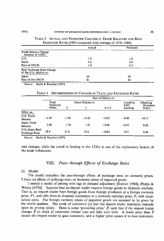
The combined effect of these changes (as a deviation from a baseline) is shown in Table

1. The effect is that the dollar appreciates sharply and the U.S. trade balance worsens

significantly as a percent of GNP. In Table 2, the predicted effects on the trade balance,

dollar exchange rate, and the short-term real interest rate are compared with the actual

effects observed between 1978-80 and 1985. The model does quite well in explaining the

shifts in the U.S. and Japanese trade balances and the Yen-dollar exchange rate. In Table

3, the overall predicted shift in the U.S. trade balance and real bilateral exchange rates are

apportioned to the various underlying disturbances. It shows that the largest factors in

explaining the exchange rate changes are both the U.S. and Japanese fiscal policies, and

that the offsetting monetary policy accounts for about 20 percent of the exchange rate changes.

.AS for the U.S. and Japanese trade balance changes, the largest explanatory factor is the

fiscal policy in the own country. Cross-country effects play a small role for the U.S., though

a fairly important role for Japan. The cutoff in lending to the LDCS accounts for about

20 percent of the trade balance shift in the evolution of each country's trade imbalances.

TA肌E1

　　　　　HlTOTs∪眺sHl　jOURNA［0F　cOMwRcE　AND　MAN＾G旧M酬τ　　　　　　　　口）ecemb6r

1981＿1985GL0BAL　ScBNARIo　wITH　Mo㎜Y　STABluzING　EMpL0YM酬丁

1981　　　　　　　　　1982 1983　　　　　　　　1984　　　　　　　　1985

U．S．1≡conomy

Output

P正iv．Consumption

Priv．Inv6stment

Govt．ConsumptionExports

Imp0fts

ImportS（quant．）

丁正ade〕Balance

Labor　DemandIn丘atiOnInt．Rate（sh）

Int．Rate（Ig）

Tobin’s　Q

Real　Exchange　Rate　　　　S／eCu

　　　　＄／yen

　　　　＄／C㎜

％

％GNP％GNP％GNP％GNP％GNP％GNP％GNP％

DDD％

％

％

％

一0．OO

　1，50

　0，27

　0．00

－O．91

　0，55

　0．86

－1，46

　0．05

－O．75

＿2．45

－0．83

－O．49

＿14．52

－20．98

－5．94

　O．07　　　　　　　　0，08

　2，89　　　　　　　　　3，38

　0．08　　　　　　　＿O．04

　0，00　　　　　　　　0．OO

－O．96　　　　　　　－1，08

　0，61　　　　　　　　0，69

　1，93　　　　　　　　2．19

－1．57　　　　　　　－1，77

　0，05　　　　　　　　0．05

－2．19　　　　　　　＿2．52

＿3，98　　　　　　　－3．09

－0．64　　　　　　　－O．37

＿1，10　　　　　　－3．16

＿15，65　　　　　　　－17．60

－23．74　　　　　　　－27．40

　－5．75　　　　　　　　－6．44

　O．05　　　　　　　　0，01

　3，66　　　　　　　　　3．59

＿O．14　　　　　　＿0，17

　0，00　　　　　　0．00

＿1．15　　　　　　　＿1，13

　0，73　　　　　　　　0，71

　2，33　　　　　　　　2．27

－1．88　　　　　　　　＿1，84

　0，04　　　　　　　　0．03

－2．68　　　　　　　－2．56

＿1．50　　　　　　　－1．50

＿O．17　　　　　　　＿0．09

－4．49　　　　　　　＿4．49

一18．63　　　　　　＿18．11

＿29．63　　　　　　－28，96

　－6．60　　　　　　　－6．40

ROECD　EconomiesOutput

Priv，ConsumptionPriv．Investment

Govt．ConsumptionExports

Imports

Imports（quant．）

Trade　Balance

Labor　DemandInHatiOn

Int．Rate（sh）

％

％GNP％GNP％GNP％GNP％GNP％GNP％GNP％

DD

一0．42

－O．45

－O．24

　0．OO

＿0．32

－0，10

－O．59

　0．14

－0，01

　0，56

　0．64

＿O．11　　　　　　　－O．17

－0．69　　　　　　　＿O．85

＿O．24　　　　　　　＿O．25

　0．OO　　　　　　　　O．O0

　0，18　　　　　　　　0．22

－O．12　　　　　　　＿O．15

＿O．63　　　　　　　　－O．70

　0，30　　　　　　　　0，37

＿O．01　　　　　　　＿O．01

　0，73　　　　　　　　0，96

　　1，30　　　　　　　　1，63

＿O．22　　　　　　　＿O．26

＿0．94　　　　　　　＿0．89

－O．24　　　　　　　＿O．23

　0．O0　　　　　　　　0，00

　0，23　　　　　　　　0．16

＿O．16　　　　　　　＿O．15

－0，73　　　　　　　＿O，70

　0，39　　　　　　　　0．31

－O．OO　　　　　　　－O．00

　　1，10　　　　　　　　1，13

　　1，71　　　　　　　　　1．63

Japanese1三conomyOutput

Priv．ConsumptionPriv．Investment

Govt．ConsumptionExports

Impo正ts

Imports（quant．）

Trade　Ba1ance

Labor　DemandInHatiOn

Int．Ratc（sh）

80〃Cα

％

％GNP％GNP％GNP％GNP％GNP％GNP％GNP％

DD

Sachs＆Roubini（1987）

一1．09

－1．58

－O．62

－O．50

　0．38

－O．20

－1，22

　1．62

－0，07

　1，13

　1．47

＿O．16　　　　　　　－0．28

－2．15　　　　　　　－2．47

－0．49　　　　　　　＿0．44

－1．00　　　　　　　－1，50

　2，00　　　　　　　　　2．38

－0．27　　　　　　　－O．33

－1．48　　　　　　　－1，75

　2，27　　　　　　　　2．71

－O．00　　　　　　　－O．OO

　O．01　　　　　　　　0，03

　2，01　　　　　　　　1．72

＿O，37　　　　　　　＿O．43

－2．34　　　　　　　＿2．30

＿O．36　　　　　　　＿0．33

＿2．20　　　　　　　＿2，20

　2，61　　　　　　　　2．52

－O．36　　　　　　　＿0．36

＿1．92　　　　　　　＿1，89

　2，97　　　　　　　　2．88

－O．00　　　　　　　－0，00

　0，05　　　　　　0，04

　0，48　　　　　　0．44

　　　　Thus，a㏄ording　to　the　Sachs＆Roubini’s　simulation　study，the　increase　in　the　U，S．

budget　de丘cits　and　the　reduction　in　the　Japanese　budget　deicits　account　for　the　greater

portion　of　both　the　dollar　appreciation　and　the　U．S．trade　dencits　md　Japanese　trade　sur－

pluses．In　addition，monetary　policy　is　one　of　the　explanatory　factors　of　the　exchange

l 9871 THEORIES OF EXCHANGE RATES DETERMINATION : A REVIEW

TABLE 2 ACTUAL AND PREDICTED CHANGES IN TRADE BALANCES AND REAL EXCHANGE RATES (1985 compared with average of 1978-1980).

Actual Predicted

45

Trade Balance Change (percent of GDP)

U. S.

Japan Rest of OECD

1.9

3.2

l.O

1.8

2.8

O. 3

Real Exchange Rate Change of the U.S. relative to :

Ja pan

Rest of the OECD

Source : Sachs & Roubini (1987)

24 41

28

18

TABLE 3 DECOMPOSITION OF CHANGES IN TRADE AND EXCHANGE RATES

Sum of Effects of:

Total Predicted

Effect U

Fiscal Policies in

J R+C

Cutoff in

LDC Lending

Offsetting

Monetary Policy

Effect on :

U.S. Trade Balance ~ I . 84 Japan Trade Balance 2. 8 8 U.S.-Japan Real Exchange Rate 28.9

Source :

- I .Ol

1.36

11.8

Sachs & Roubini (1987)

-O.23

l.91

10.6

-0,03

-0.06

-0,03

-0.40

-0.61

-O. 1 1

-O. 1 7

0.28

6.64

rate changes, while the

the trade imbalances.

cutoff in lending to the LDCS is one of the explanatory factors of

VIII Pass through E ects o Exchange Rates . - ffl tf (1) Model

The model considers the pass-through effects of exchange rates on domestic prices.

I focus on effects of exchange rates on domestic prices of imported goods.

I extend a model of pricing with lags in demand adjustment [Dohner (1984), Phelps &

Winter (1970)]. Suppose that an import trader imports foreign goods to domestic markets.

That is, an import trader buys foreign goods from forelgn producers at a foreign currency

price, P*, and sells them to domestic consumers at a domestic currency price, P, with trans-

action costs. The foreign currency prices of imported goods are assumed to be given by

the world markets. The stock of customers (x) that the import trader maintains depends

upon its pricing policy. There is some 'prevailing price,' P~, such that if the import trader

charges P its stock of customers neither rises nor falls over time. A Iower price than p

causes the import trader to gain customers, and a higher price causes it to lose customers.

46 HrroTSUBASHI JOURNAL OF COMMERCE AND MANAGEMENT [December

It is assumed that the flow of customers caused by the pricing p,olicy is proportional to the

import trader's stock of customers, a measure of the import trader's 'presence' in the market,

and that there are diminishing returns to price reduction in customer aquisition. The cus-

tomer adjustment assumptions are summarized as following:

(70) ;t=6(P;P)x; 6(P;P)=0: 6'

Assume that the import trader can rationally expect how the prevailing price, P, will

respond to disturbances in a steady state. For simplicity, assume that all import traders

are alike, and, in particular, share customers equally in the initial state.

Each customer purchases an amount v(P), which is a decreasing function of price, so

that the flow rate of sales of the import trader is xv. It is assumed that marginal revenue

from current customers is decreasing in quantity and convex to the origin.

(71) V'

The import trader's trading is done according to a decreasing returns to scale produc-

tion function and the transaction costs are assumed proportional to the domestic price of

imported goods. Thus, the transaction cost is:

(72) Pc(xv(P)), c'>0, c">0.

Assume that the import trader maximizes discounted real net revenue, and that payment

is received immediately. In other words, the import trader maximizes

J~e~'t { I / P(t)} ･[(P(t) - E(t)P*)x~(P) - P(t)c(xv(P))]dt.

Normalizing P * (=1) and taking logarithms of P and E, we can rewrite :

J~

(73) e~'t[(p - e)xv(p) - ip(x~(p))]dt.

We can write the import trader's maximization problem as :

Maximize J"

(74a) o e~'t[(p - e)xv(p) - c(xv(p))]dt

subject to

(74b) ;t=6(p;p)x

and

(74c) x(O) =xo,

where xo is the import trader's initial stock of customers.

Eq. (74) defines a dynamic optimization problem which may be solved using optimal

control techniques. It is notationally convenient to define the following functions :

F(x, p ; e) =(p - e)x~(p) - c(x~(p)),

G(x, p ; p) = 6(p ; p)x,

H(x, p, q; e, p)=F(x, p ; e) + qG(x, p; p).

where the function H is the Hamiltonian, and q is the value, or shadow price, of additional

customers. (In mathematical terms, this shadow price is the derivative of the maximized

1987] THEORIES OF EXCHANGE RATES DETERMINATION : A REVIEW 47

integral with respect to the stock of customers, x.)

Then the problem posed may be rewritten: Maximize J=

(74a') V= o e~"F(x, p; e)dt

subject to

(74b') ;t=G(x, p;p)

and

(74c') x(O)=xo'

Pontryagin-type necessary conditions are: If p(t) is an optimal time path of the import

trader's price, then there exists a function of time, ~(t), defined for t;~O, such that for each

t ~0,

(75a) p(t) mazimixes H(;t(t), p, ~(t)) with respect to p,

~(t) satisfies the differential equation

(75b) q=r~-Hx. Here the function i~(t) satisfies the differential equation

(75c) ;t=G(~t(t), p(t); p)

with initial condition x(O)=xo'

If the maximum in (75a) occurs at a p > O, we must have

Hp(jt(t), p(t), ~(t))=0,

identically in t. Translating this condition, (75b), and (74b') back into the original nota-

tion, we have the following equations that must be satisfied by an optimal triple ;t(t), p(t),

~(t) :

(76a) ~'[(p-e)-c'+~/v']+qa'=0,

(76b) c=rq-[v{(p-e)-c'} +q6],

(76c) ;~=Sx,

or

(76a') Hp(x, p, q;e, p)=0,

(76b') ~=rq-Hx(x, p, q; e, p),

(76c') ;t=G(x,p;p).

Since time does not neter explicitly in the functions F.(x, p) and G(x, p), an optimal

pricing policy p(t) for problem (74'~ actually depends on time only through jt(t). That is

assuming there exists a unique p^(t).solving (74'), theie is some function ip(x) such that

p(t)=ip(~~(t)) . , , '. ' ' characterizes not only the solution to the'problem (74'), but also the solutions to all variants

of (74') that are obtained by (a) changing 'the startin~ time,from O to an arbitrary To' or (b)

changing the initial condition on x. ' Given that thls is true of p(t), it,is clear.f.rom (.76a)- th~t it is also true of ~(t). There is

48. HITOTSUBASHI JOURNAL OF COMMERCE AND MANAGEMENT [December

a function It(x) such that

~(t)=1r(ie(t)).

Given the function x(x), the pricing rule ip(x) is defined by

(77) Hp(x, ip(x), Ir(x))=0.

Thus we have

(78) c'(x)=-[Hpx+Hpq'lr(x)]/Hpp>0

and c(X)fP-Therefore, the price determined by

P(t) = c(x(t))

(79) Jt=a(p(t))x(t)

x(O) =xo

with auxiliary variable

(80) q(t)=1r(x(t))

is optimal.

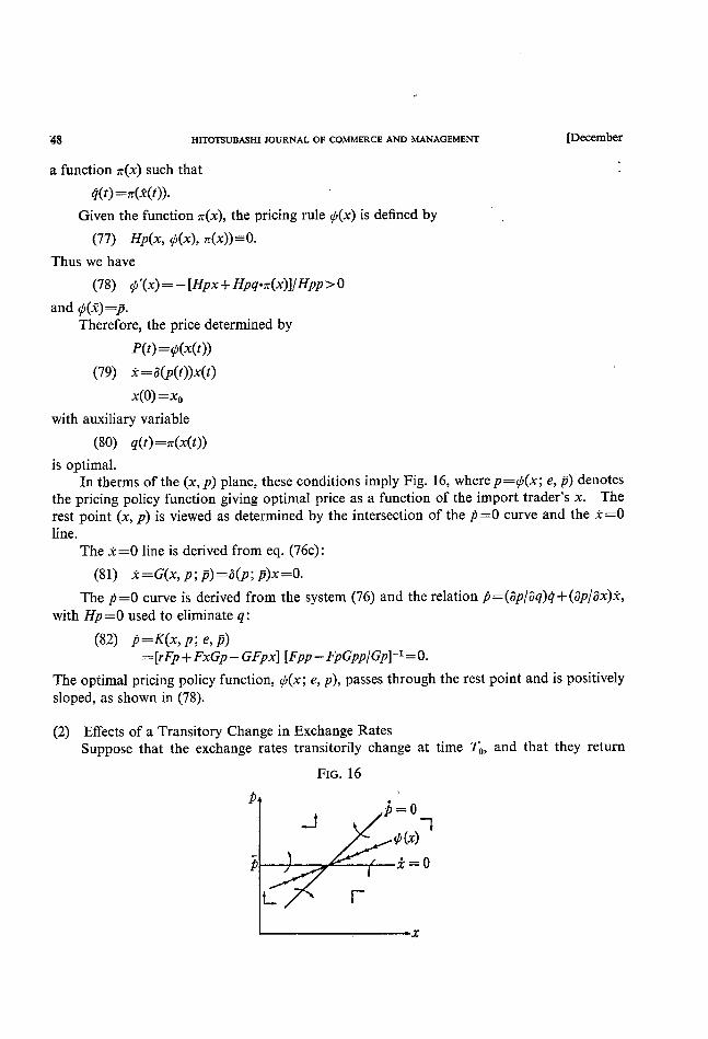
In therms of the (x, p) plane, these conditions imply Fig. 16, where p=c(x; e, p) denotes

the pricing policy function giving optimal price as a function of the import trader's x. The

rest point (x, p) is viewed as determined by the intersection of the p =0 curve and the Jt =0

line.

The ;t=0 Iine is derived from eq. (76c) :

(81) ,t=G(x,p;p)=~(p;p)x=0.

The p=0 curve is derived from the system (76) and the relation p=(aplaq)q +(ap/ax);t,

with Hp=0 used to eliminate q:

(82) p=K(x, p;e, p) =[rFp + FXGp - GFpx] [Fpp - FpGpp/Gp]~1 = O.

The optimal pricing policy function, 9'!(x; e, p), passes through the rest point and is positively

sloped, as shown in (78).

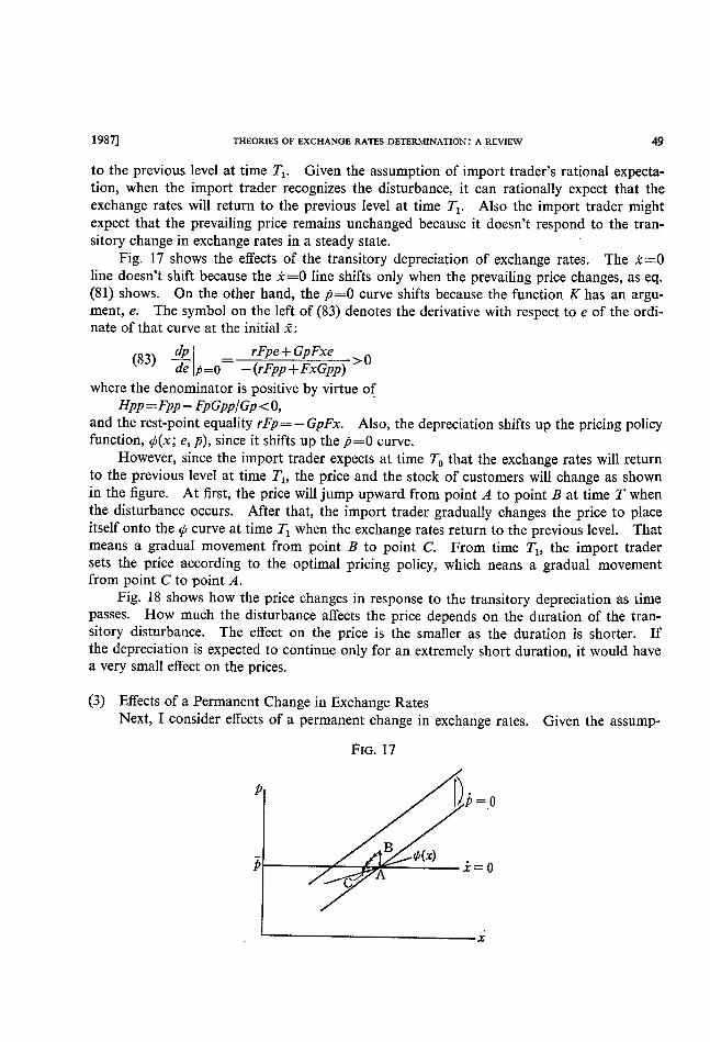
(2) Effects of a Transitory Change in Exchange Rates Suppose that the exchange rates transitorily change at time To' and that they return

FIG. 16

1

i=0

x

1987] THEORJES OF EXCHANGE RATES DETERMINATION : A REVIEW 49

to the previous level at time T1' Given the assumption of import trader's rationa] expecta-

tion, when the import trader recognizes the disturbance, it can rationally expect that the

exchange rates will return to the previous level at time Tl ' Also the import trader might

expect that the prevailing price remains unchanged because it doesn't respond to the tran-

sitory change in exchange rates in a steady state.

Fig. 1 7 shows the effects of the transitory depreciation of exchange rates. The ;t =0

line doesn't shift because the ;t=0 Iine shifts only when the prevailing price changes, as eq.

(81) shows. On the other hand, the p=0 curve shifts because the function K has an argu-

ment, e. The symbol on the left of (83) denotes the derivative with respect to e of the ordi-

nate of that curve at the initial j~ :

(83) ~~ _ rFpe+GpFxe >0 de p=0~ -(rFpp+FxGpp)

where the denominator is positive by virtue of

Hpp =Fpp - FpGpp/Gp and the rest-point equality rFp=-GpFx. Also, the depreciation shifts up the pricing policy

function, ip(x; e, p), since it shifts up the p=0 curve.

However, since the import trader expects at time To that the exchange rates will return

to the previous level at time T1' the price and the stock of customers will change as shown

in the figure. At first, the price will jump upward from point A to point B at time T when

the disturbance occurs. After that, the import trader gradually changes the price to place

itself onto the c curve at time T1 when the exchange rates return to the previous level. That

means a gradual movement from point B to point C. From time T1' the import trader sets the price according to the optimal pricing policy, which neans a gradual movement from point C to point A.

Fig. 18 shows how the price changes in response to the transitory depreciation as time

passes. How much the disturbance affects the price depends on the duration of the tran-sitory disturbance. The effect on the price is the smaller as the duration is shorter. If

the depreciation is expected to continue only for an extremely short duration, it would have

a very small effect on the prices.

(3) Effects of a Permanent Change in Exchange Rates

Next, I consider effects of a permanent change in exchange rates. Given the assump-

FIG. 17

p

f)b = o

~

B c(x)

c A i=0

x

50 HITOTSUBASHI JOURNAL OF COMMERCE AND MANAGEMENT [December

tion of import trader's expectation, the import trader perfectly foresees that the prevailing

price in' the steady state will be affected by the permanent change in exchange rates Given

the law of one price in a steady state, the steady state effect on the prevailing price is :

(84) dp~ =1 (~

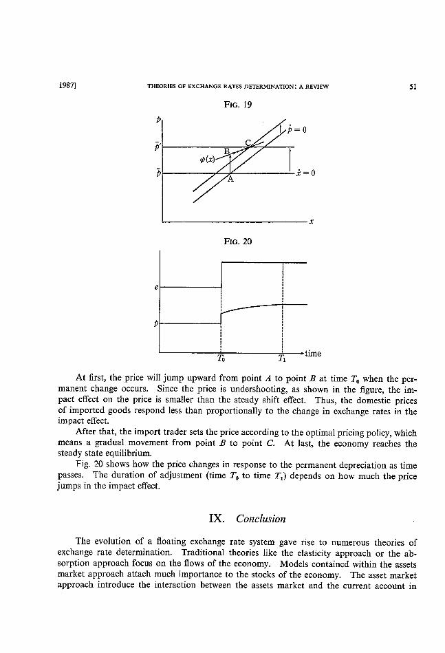
Fig. 19 shows effects of a permanent depreciation of exchange rates. The depreciation

shifts both ,t=0 Iine and p=0 curve upward.

(85) ~li=0=1

(86) dp dp dp dp~ = p=0 + '=0 de dp~=0 dp~ de p=0 dep rFpe+GpFxe + GppFx-Gp(Fpx-Fx/p~) rFpp + FXGpp rFpp + FXGpp r(Fpp + Fpe) + Gp(Fpx + Fex - Fx/p)

1 rFpp + FXGpp

Eq. (85) shows the size and direction of the shift of the ;t=0 Iine. Since eq. (85) is equal

to eq. (84), the ;t=0 Iine shifts as much as the steady state effect on the prevailing price. On

the other hand, eq. (86) shows the size and direction of the shift of the p=0 curve. Since

the second term is positive, eq. (86) is less than one. That is, the upward shift of ;t=0 Iine

is greaier than that of p =0 curve.

Though there is probability that dp/del;=0

should shift upward in response to the permanent change in exchange rates. Eq. (87) denotes the derivative with respect to e of the ordinate of the function at the initial j~:

dp dp dpdp~ (87) = ep(x) + de ip(*) de dp~'=0 dp~ de ip(x)

_ Fpe+ Fp(Gpp/Gp+ l/p~) >0 ~ ~ Fpp - FpGpp/Gp

Therefore, the movements of exchange rates and the stock of customers are shown in Fig.

FIG. 18

e

p -

.._ _-To --' '--_ __.T2- - time

.. Tl---- -

1987] THEORIES OF EXCHANGE RATES DETERMINA11:ON : A REVIEW

FIG. 19

カ一グ一力

1トOC

Bψ（功

1、工＝1

A

■

x:=0

x

51

FIG. 20

e

p

To Tl time

At first, the price will jump upward from point A to point B at time To when the per-

manent change occurs. Since the price is undershooting, as shown in the figure, the im-

pact effect on the price is smaller than the steady shift effect. Thus, the domestic prices

of imported goods respond less than proportionally to the change in exchange rates in the

impact effect.

After that, the import trader sets the price according to the optimal pricing policy, which

means a gradual movement from point B to point C. At last, the economy reaches the steady state equilibrium.

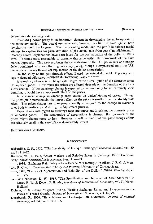
Fig. 20 shows how the price changes in response to the permanent depreciation as time

passes. The duration of adjustment (time To to time T1) depends on how much the price jumps in the impact effect.

IX. Conclusion

The evolution of a floating exchange rate system gave rise to numerous theories of

exchange rate determination. Traditional theories like the elasticity approach or the ab-

sorption approach focus on the flows of the economy. Models contained within the assets

market approach attach much importance to the stocks of the economy. The asset market

approach introduce the interaction between the assets market and the current account in

52 HrroTSUBASHI JOURNAL OF COMMERCE ANI)'MANAGEMENT [December

determining the exchange rate. ' _ Purchasing power parity is an important element in determiping the exchange rate in

the monetary model. The actual exchange rate, however, is often off from ppp in both

the short-run and the long-run. the 9ve~shooting model and t~e portfolio-balance model

attempt to explain this long-run -deviation of the -actual fate ftol~1 ppp ("misalightment").

Recently several explanations have been giveh .for th~'pvervaluation of the dollar in 1981-

1985. It seems most reasonable_ _tp__examjn=e' 'this issup wi;hin_the framework of the asset

market approach. This view attributes the overvaluation to the ~J.S. policy mix of a budget

deficit combined with an offsetting monetary policy; though I :emphasized only the U.S.

budget deficit in my theoretical explanation of the dollar appreciation.

On the study of the pass-through effects, I used the extended model of pricing with

lags in demand adjustment to~~de~r"I'~v~e~~~fh-e~fio~dl:~o~Wi~r~r~e~ults r~~ ~~ ~'~~

A transitory change in exchange rates might cause a small jump of the domestic prices

of imported goods. How much the prices are ~affected depends on the duration of the tran-

sitory change. If the transitory qh~nge is expected to continue only for an extremely short

duration, it would have a vefy'~mall ~effect ~n~{he prices. . A permanent change in exchange rates causes an undersh~oting of prices. Though

the prices jump immediately, the iippact effect on the prices is smaller than the stready state

effect. The prices change lpSs than proportionally in respond to the change in exchange

rates both immediately and duringi the adjustment process. , Expectations with regard to eichange rates afe important in pricing the domestic prices

of imported goods. If the assu~rption of expectations is changed, the dynamics of the prices might change more or less: However, it iv, ill be true that the pass-through effects

are relatively small in the case ~of-~low demand-'aidj~stment.

HITOTSUBASHI UNIVERSITY

REFERENCES

Bickerdike, C. F., 1920, "The Instability of Foreign Exchange," Economic Jou,'nal, vol. 30,

no. 1: 118-22. Branson, W. H. 1977, "Asset Markets and Relative Prices in Exchange Rate Determina-

'

tion," Sozialwissenschaftlic/1e Annalen, Band I : 69-89.

1984 "Exchange Rate Policy after a Decade of Floatmg"' m Bilson J F. O. & Mars-

ton, R. C. eds., Exchange Rate Theory and Practice, University of Chicago Press.

1985, "Causes of Appreciation and Volatility of the Dollar," NBER Working Paper,

no. 1777. & Henderson. D. W., 1985, "The Specification and Influence of Asset Markets," in

Jones. R. W. & Kenen, P. B. eds., Handbook oflnternationa/ Economics, vol. II, North-

Dohner R S (1984) "Export Pncmg Flexible Exchange Rates and Drvergence m the Prices of Traded Goods," Journal of Internatlonal Economics, vol. 16, 79-lOl.

Dornbusch, R., 1976, "Expectations and Exchange Rate Dynamics," Journal of Political

' Economy, vol. 84, no. 6: 1 161-76.

19871　　　　　　　　　　丁朋0R皿≡s0HxcHANGE　M1珊D飢駅MIMTI0N　A　REwEw　　　　　　　　　　　　53

’［，1980，0ρθ〃万ω〃o加γ〃oぴoθω〃o〃fω，Basib　Books．一

＿r1983，“Excha㎎e　Rate　Economics：Where　Do　We　Stand？，”in　Bhandari，J．．S．＆Put－

　　nam，B．H．eds．，及oわo〃c〃2〃％〃此〃cθo〃例2肋1ε瓜c乃伽φRo蜘，MIT　Press．’

＿＿＿，1985，“Purchasing　Power　Parity，”W万ER肌o欣加gアψ〃，no．1591。．一’．

r＆Fischer，S．，1980，、“Exchange　Rateζand　the　Current　Account，’一ノ閉αたα〃肋o〃o〃c

　　－Rε切εw，vo1．70，no．51960－71．　　　　　　1、　．　　　．　　　　　　，．　　　　　　　ピ

≒＆i，1984，“The　Open　Economy：Implication　for　M6neta正y　and　Fisca1Policy，！三　　jV二8万1～肌orた加91〕αρε1‘，no．1422．

Feldstein，M．S．，1986，“The　Budget　De丘cit　and　the．Do11ar；”W万万R〃6ぴoεcoκo〃ωルー

。＝’1〃〃α11986，MIT　Press．一

F1eming，J．M。，1962，“Domestic　Financial　Poucies　unde正Fixed　and廿nder　F1oating　Ex－

　　change　Rates，”1〃FαψP卯〃，vo1．9：369＿79．

Frankel，J．A．，1983，“Monetary　and　Port㎞lio－Balance　Models　of　Excha㎎e　Rate　Deter一

　　工1ユinallion，”　in　Bhandari＆Putnam，eds．，1北o〃o〃一た1〃胞r∂ξρεη63〃c8αηゴFZεx必1ε万x－

　　c〃α〃9θ火”θふ

一，1985，“Six　Possible　Meani㎎s　of‘0vervaluation’：The1981－85Dollar，”万∬oγ3加　　11〃’21・〃o〃o〃α11サ〃o〃c3，no．159．

Frenkel，J．A．，1983，“F1rxible　Exchange　Rates，Prices，and仙e　Role　of‘News’：Lessons

　　耐om　the1970s，”in　Bhanda正i＆Putnam　eds。，肋o〃o〃c肋τε〃％ε〃帥cθα〃〃α〃ε

　　亙xo乃伽9εR〃ω。

＿＆Mussa，M．L．，1985，“AssetMarkets，Excha㎎e　Rates，andtheBalancc　ofPayments，”

　　in　Jones＆Kenen　eds．，H伽必ooκgμ〃〃〃α〃o〃o1及o〃o〃ω，vo1．II．

Fukao，M．，1983，Kαw伽ε一〃o’o　K柳狐物o（Exchange　Rates　and　Financial　Markets），Toyo－

　　keizaishinposha．

Harberger，A．C．，1950，“Currency　Depreciation，Income，and　the　Balance　ofTrade，”Jo〃閉α1

　　qグ1〕o1〃たα1万co〃o〃一γ，vol．58，no．1：47－60．

Ishii，N．，McKibbin，W．J．，＆Sachs，J．D．，1985，“Macroeconomic　Interdependence　of

　　Japan　and　the　Ul■ited　States：Some　Simulation　Results，”W万ER肋枇加g　Pηεr，no．

　　1637．

Kenen，P．B．，1985，“Macroeconomic　Theory　and　Po1icy：How　the　C1osed　Economy　was　　Opened，”Jones＆Kenen　eds．，∬閉励ooんg1肋仰〃o〃o”α1五coκo〃ω，vo1，II．

Kouri，P．J．K．，1976，“T11e　Exchange　Rate　and　the　Balance　of　Payments　in　the　Short　Run

　　andintheLongRun：AMonetaryApproach，”8c伽砺〃〃わ〃∫o〃閉olgグZω〃o〃c3，　　vo1．78，no．2：280＿304．

McKbbin，W．J．＆Sachs，J．D．，1986，“Comparing　the　G1oba1Performance　of舳emativc　　ExchaIige　Arrangements，”」V丑ER肋脈加g　Pη〃，no．2024．

Munde1l，R．A．，1963，“Capita1Mobi1ity　and　Stabi1ization　Policy　under　Fixed　and　F1exible

　　E・ch・㎎eRat・・，”Cα・α励伽■・・閉α1ぴ肋…〃・”〃P・1肋6α18・加・oε，vo1129，m．

　　4：475＿85．

Niehans，J．，1984，肋炊〃α〃o〃α1〃o〃θ〃γ及o〃o〃c3，Johns　Hopkins　University　Press．

Obst㈲d，M．，1985，“Hoating　Excha㎎e　Rates：Experience　and　Prospects，”〃oo〃〃g∫P螂r∫

　　0〃1；c0腕0〃2た■4cガ切’γ，2：369－450．

＿＆Stockman，A．C。，1985，“Exchange－Rate　Dynamics，”in　Jones＆Kenen　eds．，亙伽4　　ろ00κψ〃θ閉α〃0〃α1肋0”0〃C8，VO1．II．

Phelps，E．S。＆Winter，S，G．（1970），“0ptiml　Price　Po1icy㎜derAtomistic　Competition，”

54 HITOTSUBAsru JouRNAL OF COMMERCE AND MANAGEMENT

Phelps, Microeconomic Foundations of Employment and Inflation Theory, Norton, New

York. Sachs, J. D., 1985, "The Dollar and the Policy Mix: 1985," Brookings Papers on Economic

Activity, I : I17-85.

& McKibbin, W. J., 1985 "Macroeconormc Policres m the OECD and LDC External adjustment," NBER Working Paper, no. 1534. & Roubini, N., 1987, "Sources of Macroeconomic Imbalances in the World Economy: A Simulation Approach," The Third International Conference, Institute for Monetary

and Economics Studies, Bank of Japan.

Williamson, J., 1985, The Exchange Rate System, Institute for International Economics,

Policy Analysis in International Economics, 5.