Embed Size (px)
Citation preview

THEORIES OF ECONOMIC GROWTH AND SOME
APPLICATIONSDr. Iñaki Erauskin
January 2016
Course materials atpaginaspersonales.deusto.es/ineraus/PhD.htm 1

For inspiration
• “Is there some action a government of India could take that would lead the Indian economy to grow like Indonesia’s or Egypt’s? If so, what, exactly? If not, what is it about the “nature of India” that makes it so? The consequences for human welfare involved in questions like this are staggering: once one starts to think about them, it is hard to think about anything else”.Robert E. Lucas Jr. (1988) “The mechanics of economic
development”, Journal of Monetary Economics, 22:3-42 (p. 5). Nobel Prize winner in Economics 1995. 2
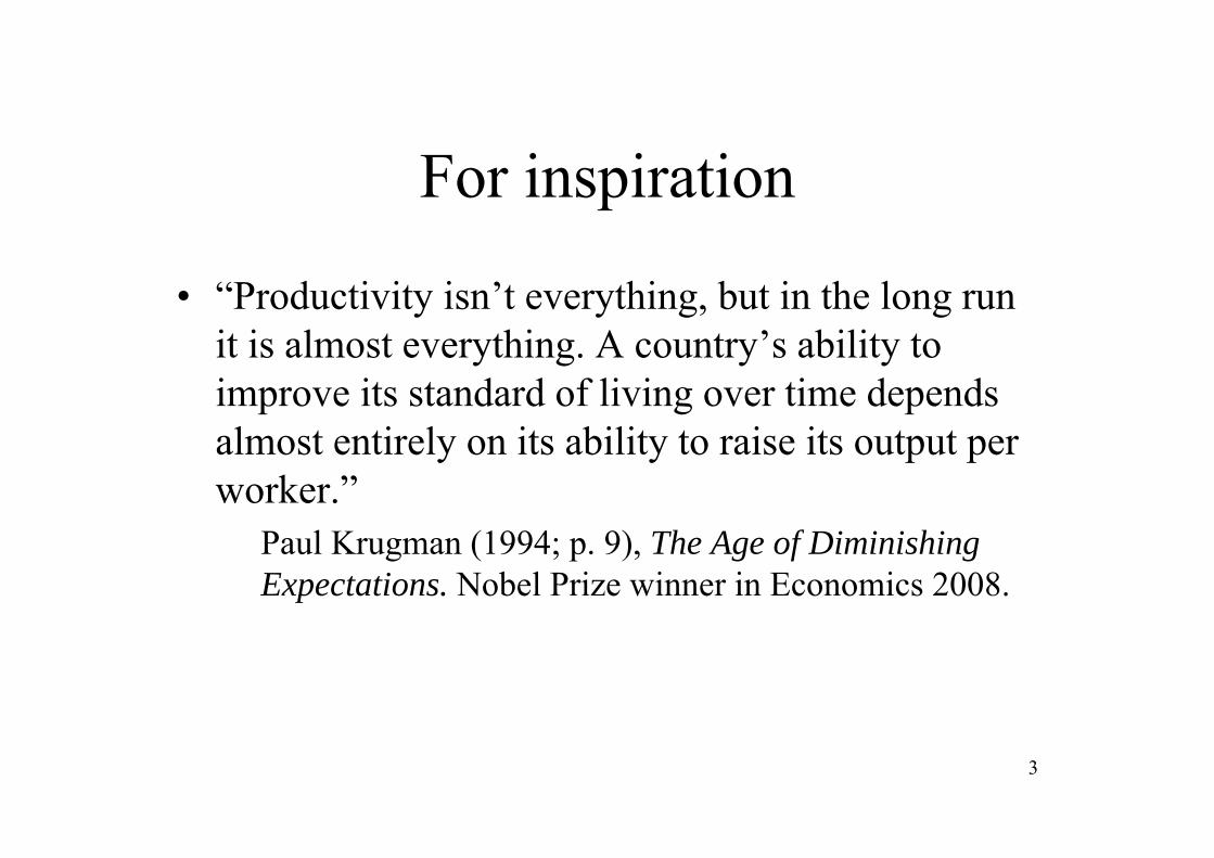
For inspiration
• “Productivity isn’t everything, but in the long run it is almost everything. A country’s ability to improve its standard of living over time depends almost entirely on its ability to raise its output per worker.”
Paul Krugman (1994; p. 9), The Age of Diminishing Expectations. Nobel Prize winner in Economics 2008.
3

INDEX
1. Introduction2. Some facts3. Three waves (Five models):
– 1st wave: The Harrod-Domar model (1)– 2nd wave: The neoclassical model (2)– 3rd wave: Endogenous models
• Investment based: The AK endogenous model (3)• Innovation based:
– The product variety model (4)– The Schumpeterian model (5) 4

INDEX
4. Empirical evidence5. Two (personal) practical examples:
– Growth accounting– Current account behavior
6. Conclusions
5

1. INTRODUCTION
6

INTRODUCTION
• Economic growth is a fundamental branch of (macro)economics.
• It focuses on the long-run trend performance of GDP growth (as opposed to business cycles).
• The literature is vast, intuitively quite simple, but mathematically demanding.
7
2. SOME FACTS
8
9
10

For discussion
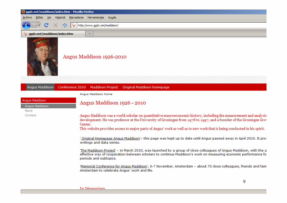
• Please look at the data provided by Angus Maddison.
• Which are the main trends shown by thedata?
• Please note “The rule of 70”: a country growing at a g rate, will double GDP per capita in 70/g years.
11

Source: Clark, Gregory (2008). A farewell to alms. A brief economic history of the world. Princeton University Press.
12

Important sources of data
• OECD: http://www.oecd.org/• IMF: http://www.imf.org/• World Bank: http://www.worldbank.org/• Eurostat: ec.europa.eu/eurostat• National Statistical Offices.
– For instance, Instituto Nacional de España (INE) for Spain: http://www.ine.es/
13
Important sources of data
• Central Banks.– For instance, European Central Bank:
www.ecb.int• EUKLEMS growth and productivity
accounts: http://www.euklems.net/– WorldKLEMS: http://www.worldklems.net/
14

Important sources of data
• Penn World Table: https://pwt.sas.upenn.edu/
• The Conference Board: http://www.conference-board.org/
15
Motivation
• OECD November 2012: “Looking to 2060: Long term global growth prospects?” – Main Paper: http://www.oecd-
ilibrary.org/economics/looking-to-2060-long-term-global-growth-prospects_5k8zxpjsggf0-en
– Short paper (policy note): http://www.oecd.org/economy/economicoutlookanalysisandforecasts/2060policynote.pdf
– Video: http://youtu.be/fnIl212tBPk
• What is your opinion, based on the data? 16
Motivation
• Robert J. Gordon: “Is US economic growth over? Faltering innovation confronts the six headwinds” (2012) – Paper:
http://www.cepr.org/pubs/PolicyInsights/PolicyInsight63.pdf– Shorter reference: http://www.voxeu.org/article/us-economic-
growth-over
• What do you think about his views?
17

Motivation
Robert J. Gordon (2012)18

Motivation
• Peter C. Evans & Marco Annunziata “Industrial internet: Pushing the boundaries of minds and machines” (2012)– Paper: http://files.gereports.com/wp-content/uploads/2012/11/ge-
industrial-internet-vision-paper.pdf– Shorter reference: http://www.voxeu.org/article/next-productivity-
revolution-industrial-internet
• Erik Brynfolsson & Andrew McAfee, “The Second Machine Age: Work, Progress, and Prosperity in a Time of Brilliant Technologies” (2014). 19
Motivation
• Kenneth Rogoff: “Rethinking the growth imperative” (2012)– Opinion: http://www.project-
syndicate.org/commentary/rogoff88/English
• What do you think about his views?
20
Motivation
• Growth versus degrowth: “Living better with less”– My own paper (2012):
http://paginaspersonales.deusto.es/ineraus/Files/ArticuloI%C3%B1akiErauskin_Decrecimiento_Completo.pdf
– Kallis, Kerschner, and Martinez-Alier: “The economics of degrowth” (2012): http://www.sciencedirect.com/science/article/pii/S0921800912003333
21
SOME FACTS
• Some facts (there are many):– Differences in the level of income, and
differences in the rate of income growth among countries.
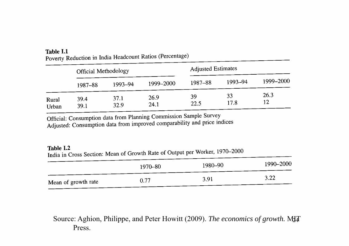
– Growth is a recent phenomenon.– “Club convergence”.– Poverty reduction. – Inequality reduction, for the world as a whole.
• But more inequality in the developed world (Piketty). 22

Source: Aghion, Philippe, and Peter Howitt (2009). The economics of growth. MIT Press.
23
Source: Aghion, Philippe, and Peter Howitt (2009). The economics of growth. MIT Press.
24
25

26

27
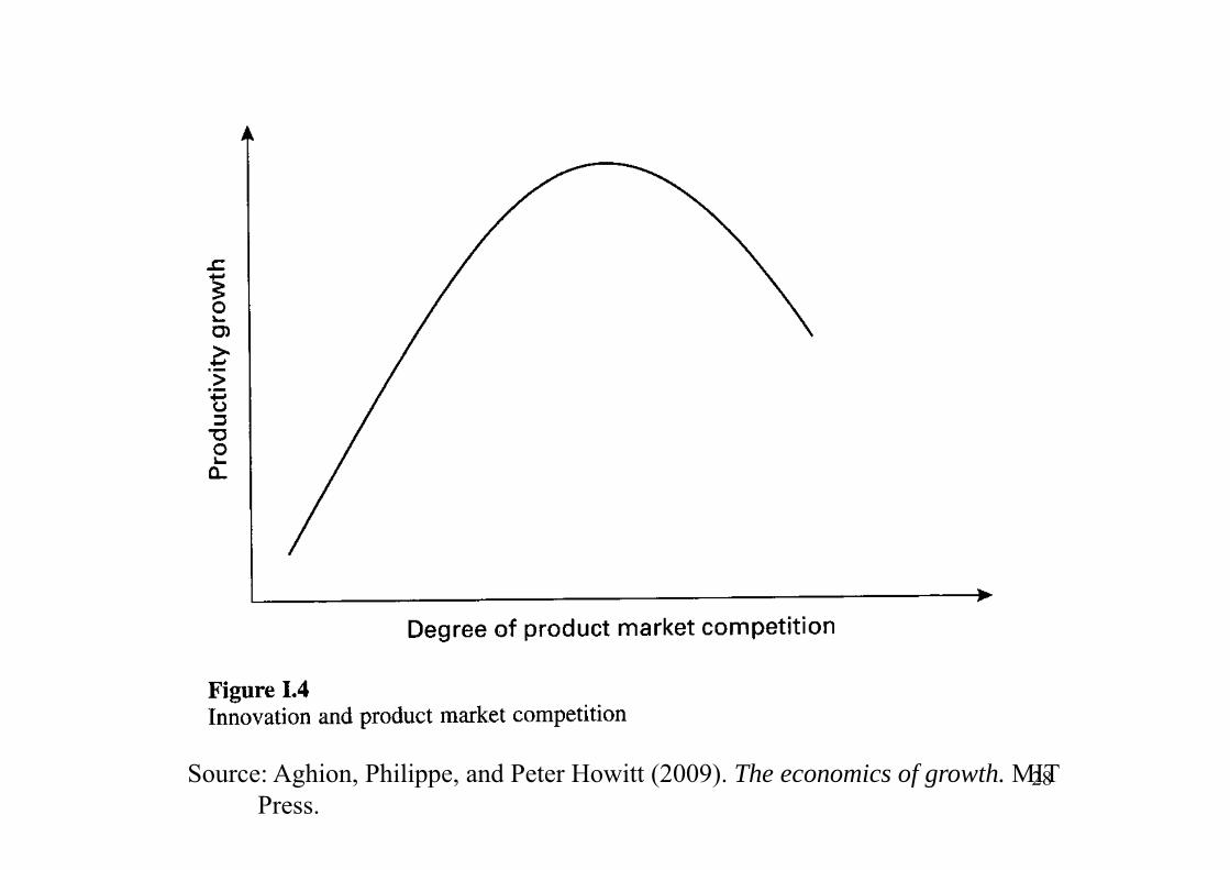
Source: Aghion, Philippe, and Peter Howitt (2009). The economics of growth. MIT Press.
28
3. THREE WAVES(FIVE MODELS)
29
THREE WAVESFIVE MODELS
• There are many frameworks to analyze economic growth. The “correct” model depends on the issue one wants to focus on.
• This module will be focused on the five main models.
• Aghion and Howitt (2009; mainly Introduction and Part I) will be the main reference in Sections 3 and 4 in this presentation. 30
3.1: THE HARROD-DOMAR MODEL
31

THE HARROD-DOMAR MODEL
• This pertains to the “first wave” in modern economic growth (Harrod 1939, Domar 1946).
• It is a Keynesian inspired growth model.– “Domar was writing in the aftermath of the Great
Depression that made many people running the machines lose jobs. Domar and many other economists expected a repeat of the Depression after World War II unless the government did something to avoid it. Domar took high unemployment as a given, so there were always people available to run any additional machines that you built.” (Easterly, 2001)
32
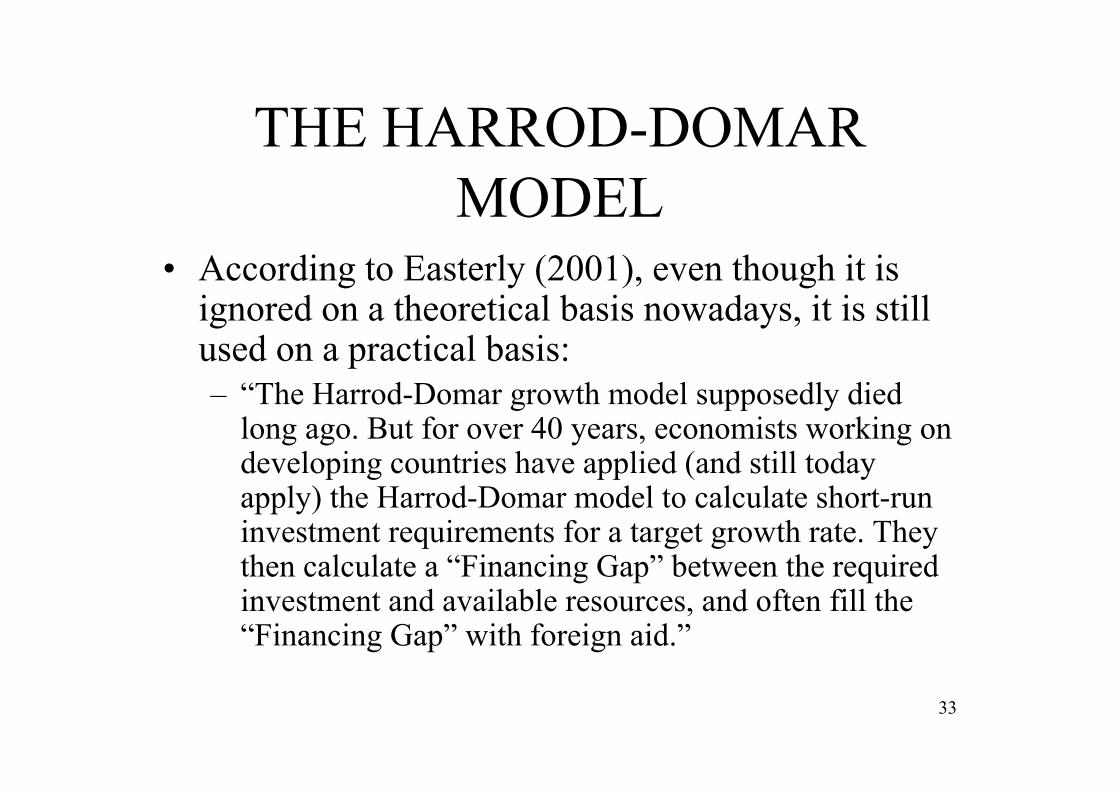
THE HARROD-DOMAR MODEL
• According to Easterly (2001), even though it is ignored on a theoretical basis nowadays, it is still used on a practical basis:– “The Harrod-Domar growth model supposedly died
long ago. But for over 40 years, economists working on developing countries have applied (and still today apply) the Harrod-Domar model to calculate short-run investment requirements for a target growth rate. They then calculate a “Financing Gap” between the required investment and available resources, and often fill the “Financing Gap” with foreign aid.”
33
THE HARROD-DOMAR MODEL
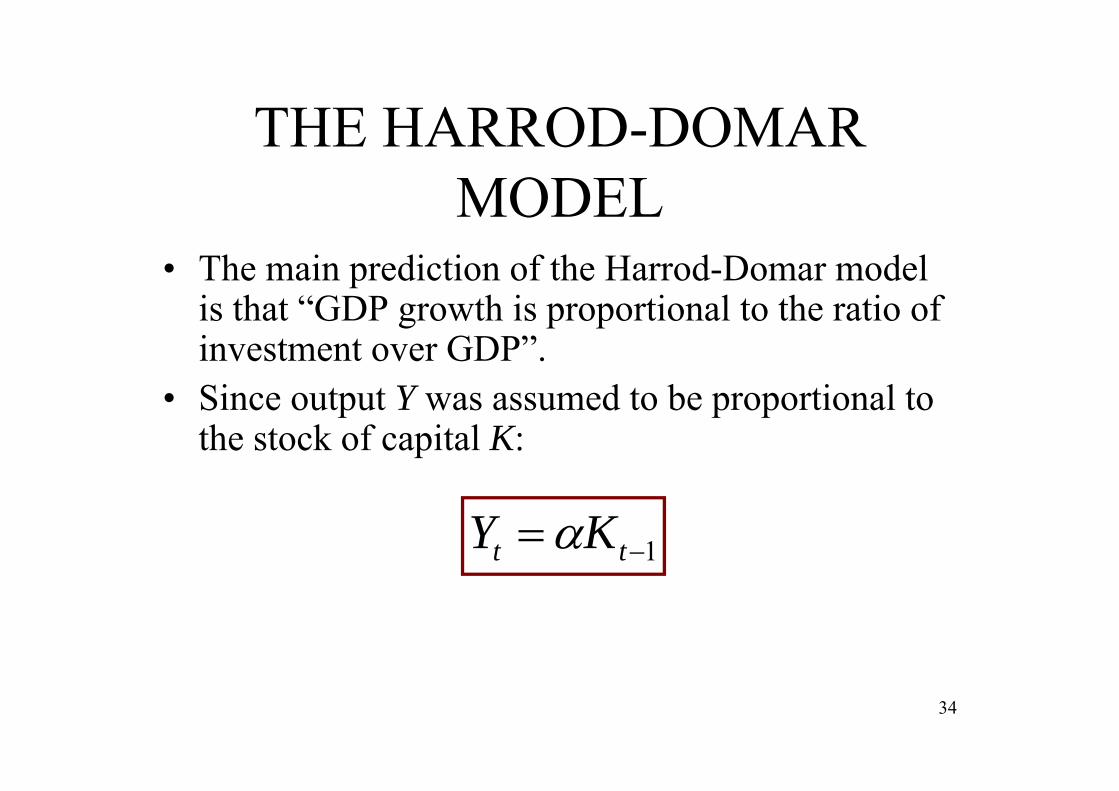
• The main prediction of the Harrod-Domar model is that “GDP growth is proportional to the ratio of investment over GDP”.
• Since output Y was assumed to be proportional to the stock of capital K:
1 tt KY
34
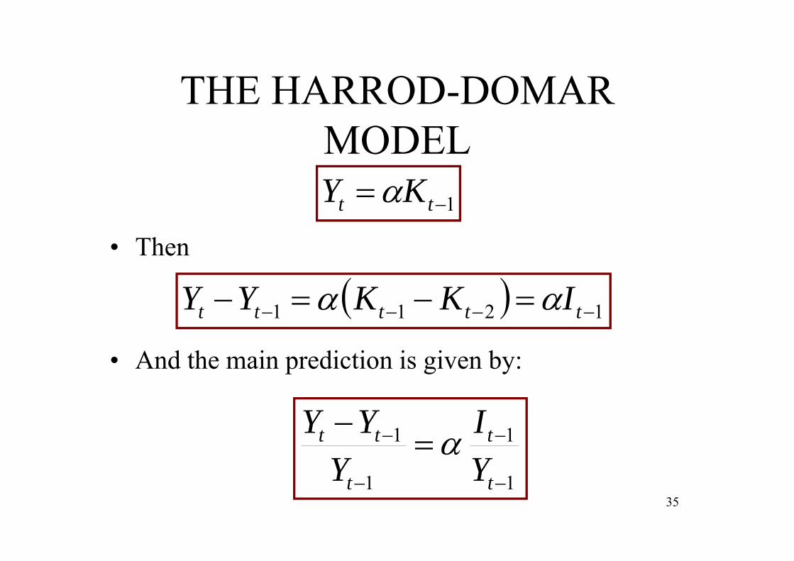
THE HARROD-DOMAR MODEL
1 tt KY • Then
1211 ttttt IKKYY
1
1
1
1
t
t
t
tt
YI
YYY
• And the main prediction is given by:
35
THE HARROD-DOMAR MODEL
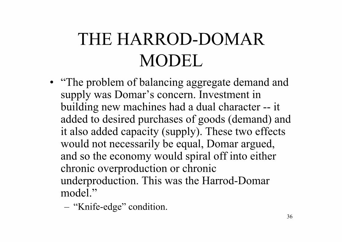
• “The problem of balancing aggregate demand and supply was Domar’s concern. Investment in building new machines had a dual character -- it added to desired purchases of goods (demand) and it also added capacity (supply). These two effects would not necessarily be equal, Domar argued, and so the economy would spiral off into either chronic overproduction or chronic underproduction. This was the Harrod-Domarmodel.”– “Knife-edge” condition.
36

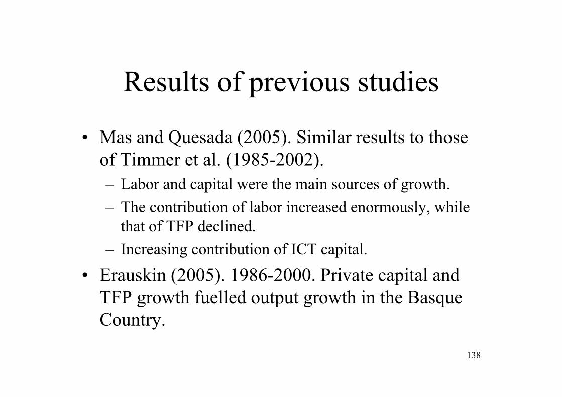
THE HARROD-DOMAR MODEL
• As we will show below, the Harrod-Domarmodel can also be seen as a special case of the AK model.
• The empirical evidence is at odds with the main predictions of the model.
37

3.2: THE NEOCLASSICAL MODEL
38
THE NEOCLASSICAL MODEL
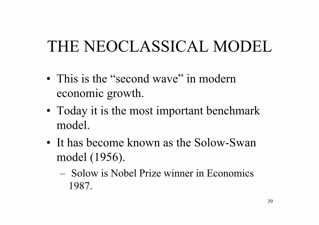
• This is the “second wave” in modern economic growth.
• Today it is the most important benchmark model.
• It has become known as the Solow-Swan model (1956).– Solow is Nobel Prize winner in Economics
1987.39

40
THE NEOCLASSICAL MODEL
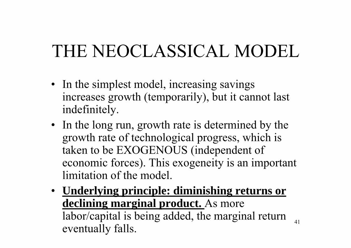
• In the simplest model, increasing savings increases growth (temporarily), but it cannot last indefinitely.
• In the long run, growth rate is determined by the growth rate of technological progress, which is taken to be EXOGENOUS (independent of economic forces). This exogeneity is an important limitation of the model.
• Underlying principle: diminishing returns or declining marginal product. As more labor/capital is being added, the marginal return eventually falls.
41
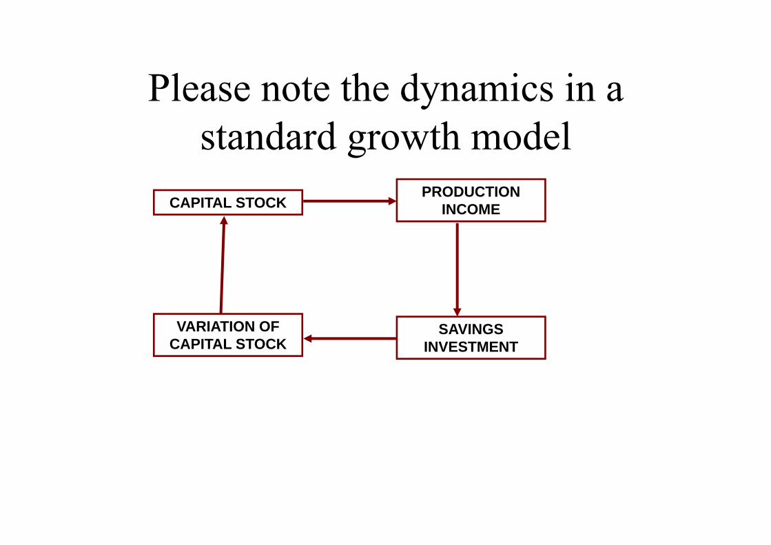
Please note the dynamics in a standard growth model
CAPITAL STOCK PRODUCTION
INCOME
SAVINGSINVESTMENT
VARIATION OF CAPITAL STOCK
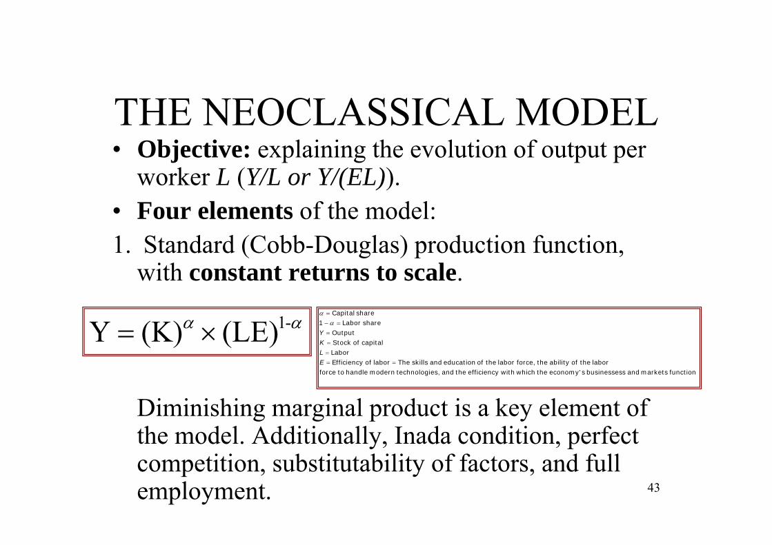
THE NEOCLASSICAL MODEL• Objective: explaining the evolution of output per
worker L (Y/L or Y/(EL)).• Four elements of the model:1. Standard (Cobb-Douglas) production function,
with constant returns to scale.
Diminishing marginal product is a key element of the model. Additionally, Inada condition, perfect competition, substitutability of factors, and full employment. 43
-1(LE)(K)Y function markets and sbusinesses seconomy' the which with efficiency the and es,technologi modern handle to force
labor the of ability the force,labor the of education and skills Thelabor of EfficiencyLabor
capital ofStock Output
shareLabor 1share Capital
ELKY
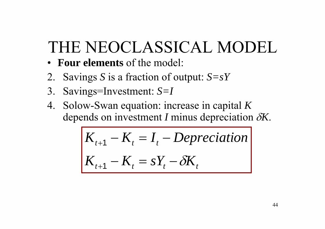
THE NEOCLASSICAL MODEL• Four elements of the model:2. Savings S is a fraction of output: S=sY3. Savings=Investment: S=I4. Solow-Swan equation: increase in capital K
depends on investment I minus depreciation K.
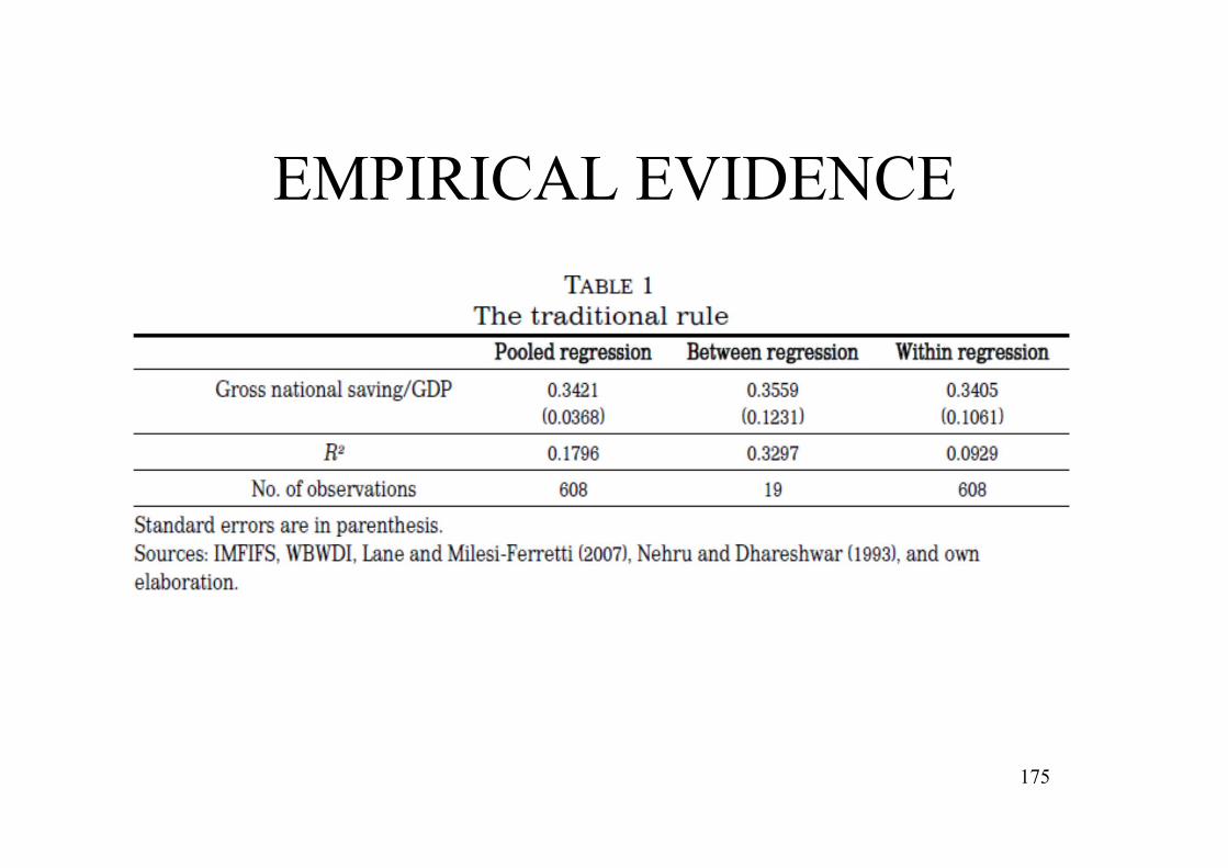
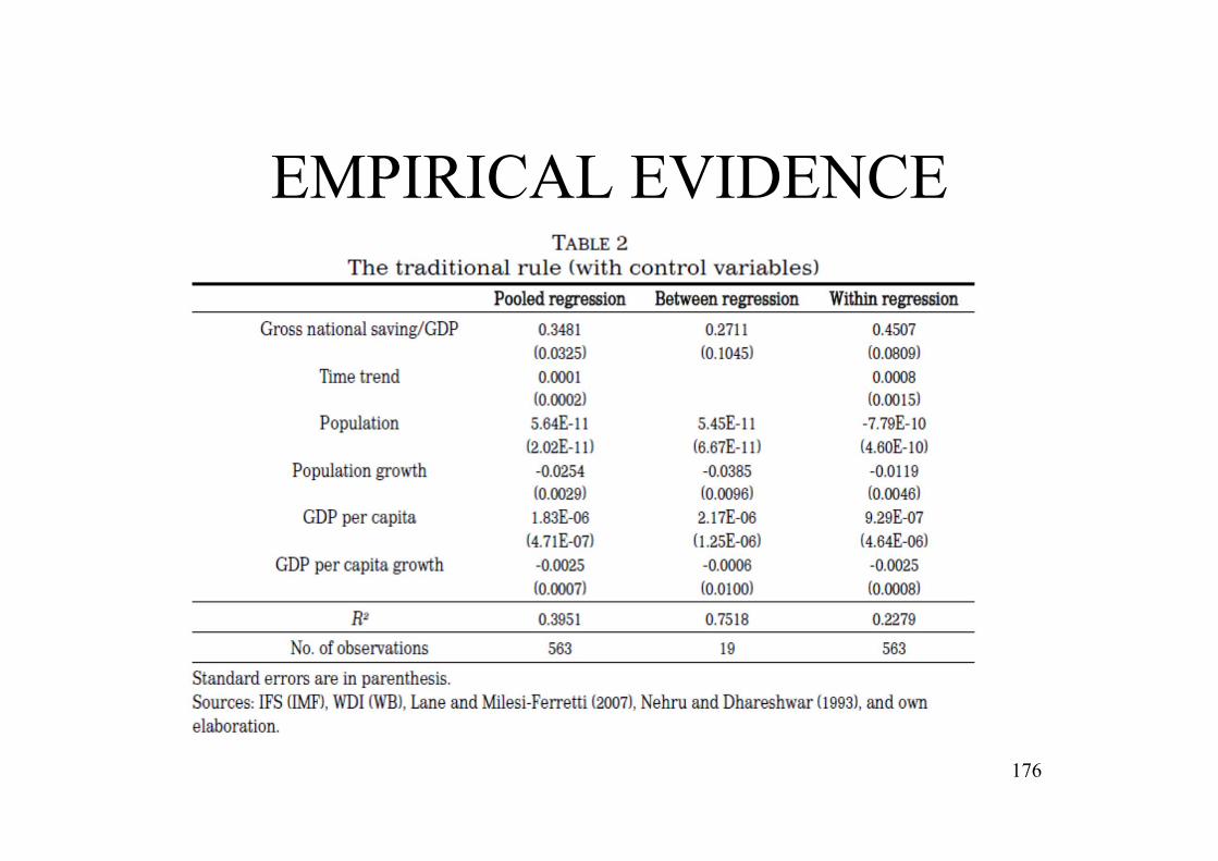
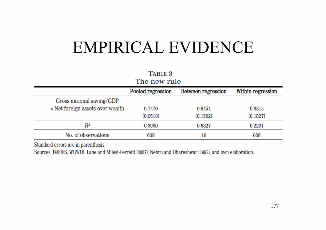
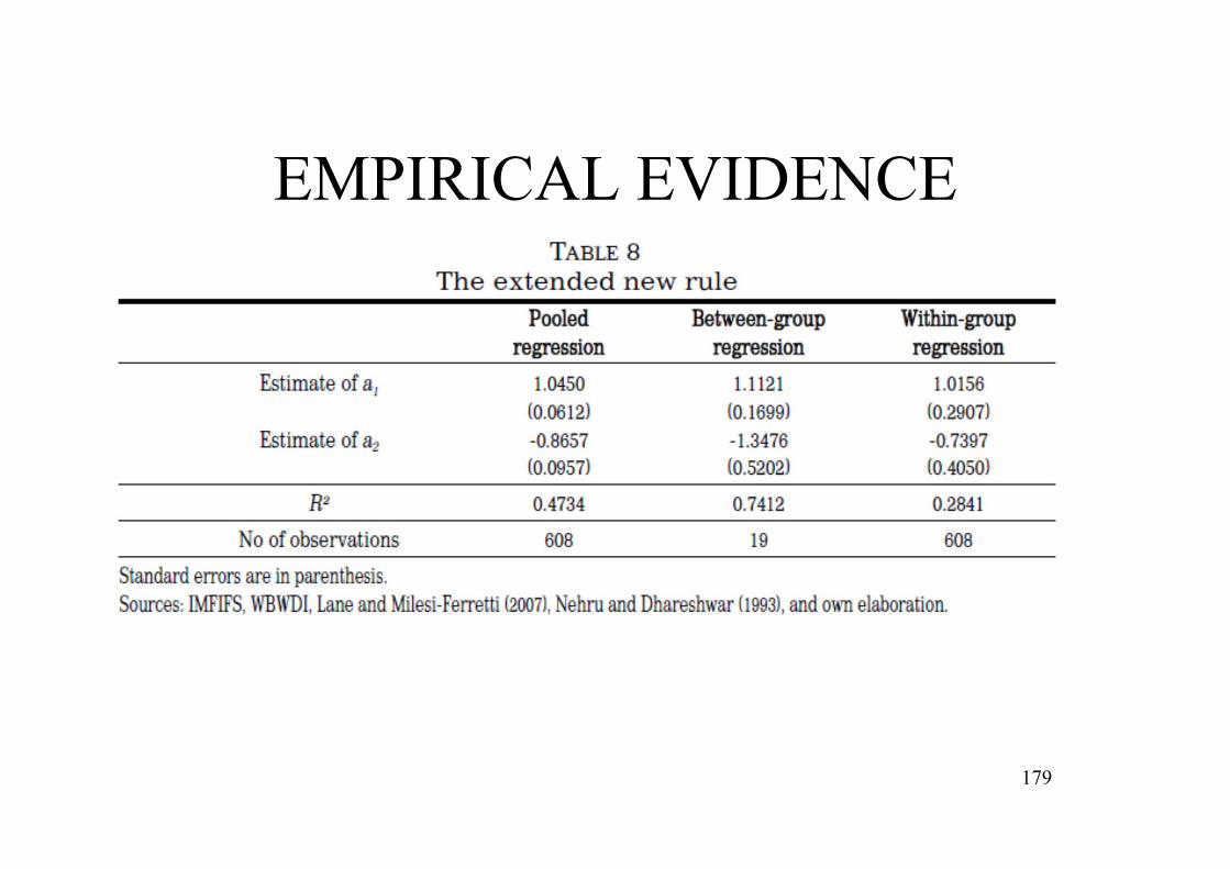
44
tttt
ttt
KsYKK
onDepreciatiIKK
1
1

THE NEOCLASSICAL MODEL
tttt kgnyskk ˆˆˆˆ1
• Then, in intensive terms (dividing by theunits of effective workers, EL), we get, after some algebra, that
tttt KsYKK 1
where n is population growth and g is therate of technological progress.
n denotes the growth rate of population N and g the growth rate of the level of technology (or efficiency of labor) E
A “hat” denotes the level of a variable in intensive terms: 45
tt
tt LE
Kk ˆ
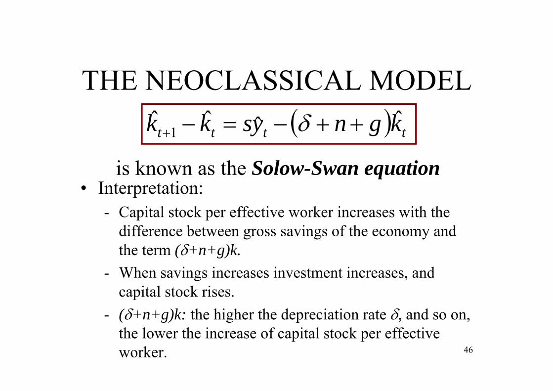
THE NEOCLASSICAL MODEL
• Interpretation:- Capital stock per effective worker increases with the
difference between gross savings of the economy and the term (+n+g)k.
- When savings increases investment increases, and capital stock rises.
- (+n+g)k: the higher the depreciation rate , and so on, the lower the increase of capital stock per effective worker.
tttt kgnyskk ˆˆˆˆ1
is known as the Solow-Swan equation
46
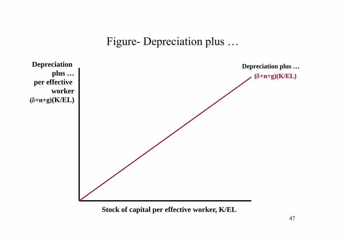
Figure- Depreciation plus …
Stock of capital per effective worker, K/EL
Depreciationplus …
per effectiveworker
(+n+g)(K/EL)
(+n+g)(K/EL)Depreciation plus …
47
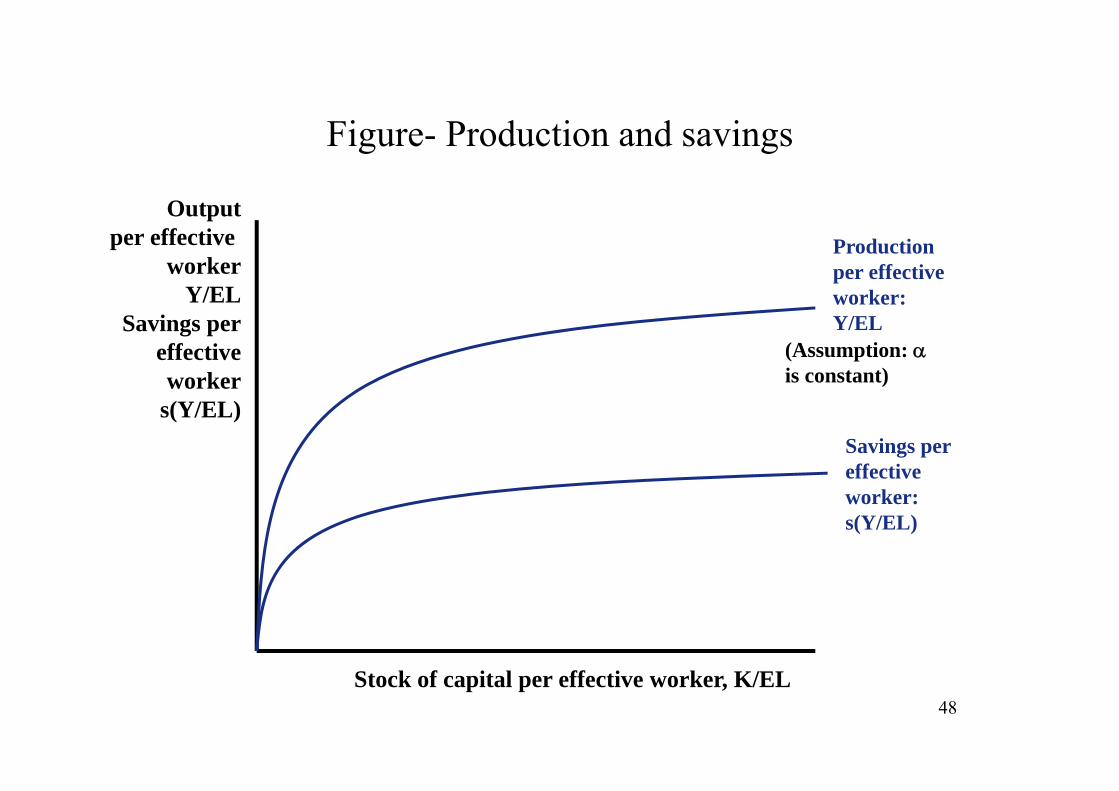
Figure- Production and savings
Stock of capital per effective worker, K/EL
Outputper effective
workerY/EL
Savings pereffectiveworker
s(Y/EL)
Productionper effectiveworker:Y/EL
(Assumption: is constant)
Savings per effective worker:s(Y/EL)
48
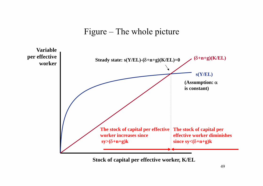
Figure – The whole picture
Stock of capital per effective worker, K/EL
Variableper effective
worker
s(Y/EL)
(+n+g)(K/EL)
(Assumption: is constant)
The stock of capital per effectiveworker increases sincesy>(+n+g)k
The stock of capital per effective worker diminishessince sy<(+n+g)k
Steady state: s(Y/EL)-(+n+g)(K/EL)=0
49

THE NEOCLASSICAL MODEL
• In a balanced equilibrium (steady state):
tttt kgnyskk ˆˆˆˆ1
gns
YK
• This implies that, after some algebra, thestock of capital per effective worker and capital-output ratio reach a steady state:
50
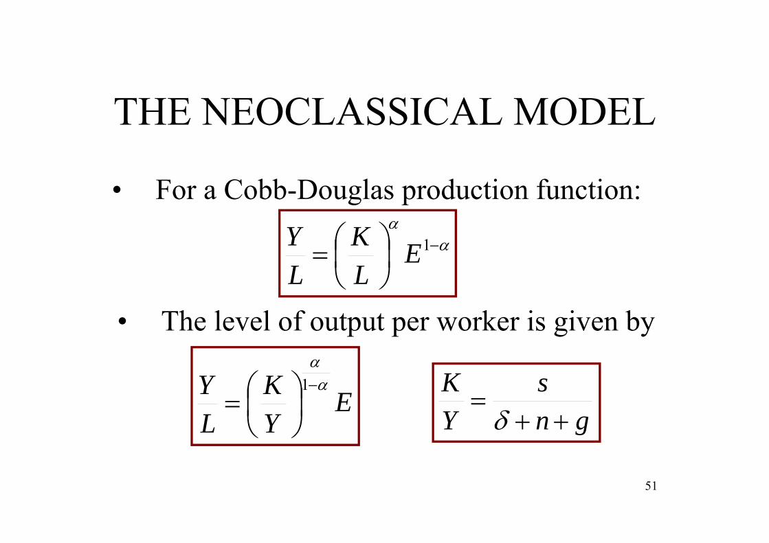
THE NEOCLASSICAL MODEL
• For a Cobb-Douglas production function:
1E
LK
LY
• The level of output per worker is given by
gns
YK
EYK
LY
1
51
THE NEOCLASSICAL MODEL
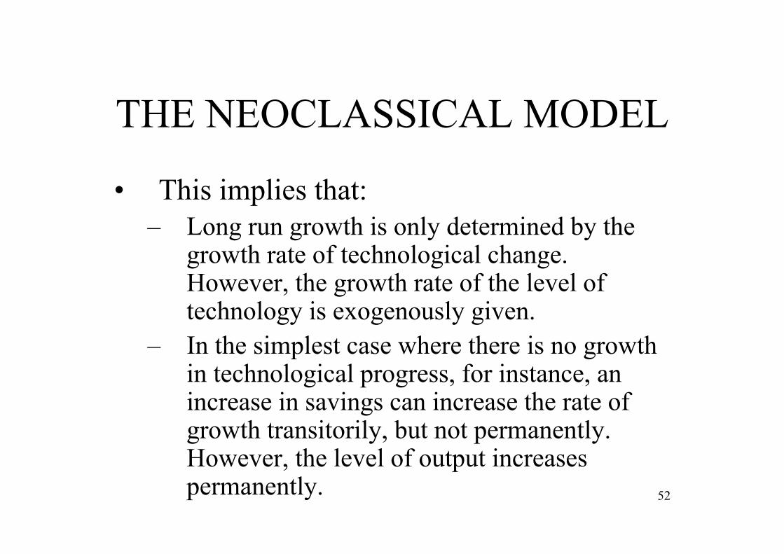
• This implies that:– Long run growth is only determined by the
growth rate of technological change. However, the growth rate of the level of technology is exogenously given.
– In the simplest case where there is no growth in technological progress, for instance, an increase in savings can increase the rate of growth transitorily, but not permanently. However, the level of output increases permanently. 52

THE NEOCLASSICAL MODEL• Based on these results, the model suggests
a testable prediction: Are poor countries likely to catch up with rich ones?
• This has become known as conditional convergence.
• If countries have the same characteristics (technology, ...), the answer is YES for the neoclassical growth model, since they will converge on the same steady state.
53

THE NEOCLASSICAL MODEL• There is a vast literature on this issue,
when compared to the AK model (more on this below).
54

THE NEOCLASSICAL MODEL
• Additionally, the neoclassical growth model offers a growth accounting framework to quantify the contribution of inputs to output growth (Solow, 1957). More on this will be shown below in Sections 4 and 5.
55
THE NEOCLASSICAL MODEL
• Please note that this model can be easily extended to incorporate an endogenous savings rate a la Cass-Koopmans-Ramsey. This is the benchmark model in advanced and PhD macroeconomics courses today.
56

3.3: THE AK MODEL
57
THE AK MODEL
• In the neoclassical growth model the rate of technological change was exogenously given. However, that was clearly unsatisfactory.
• Now this is endogenously derived.
58
THE AK MODEL
• The AK growth model pertains to the third wave (and, in turn, to the “first family” (investment based) of third-wave-models; since there are others in modern economic growth.
59

THE NEOCLASSICAL MODEL
• The neoclassical model assumes that technological change is exogenously given (determined by non-economic forces).
60
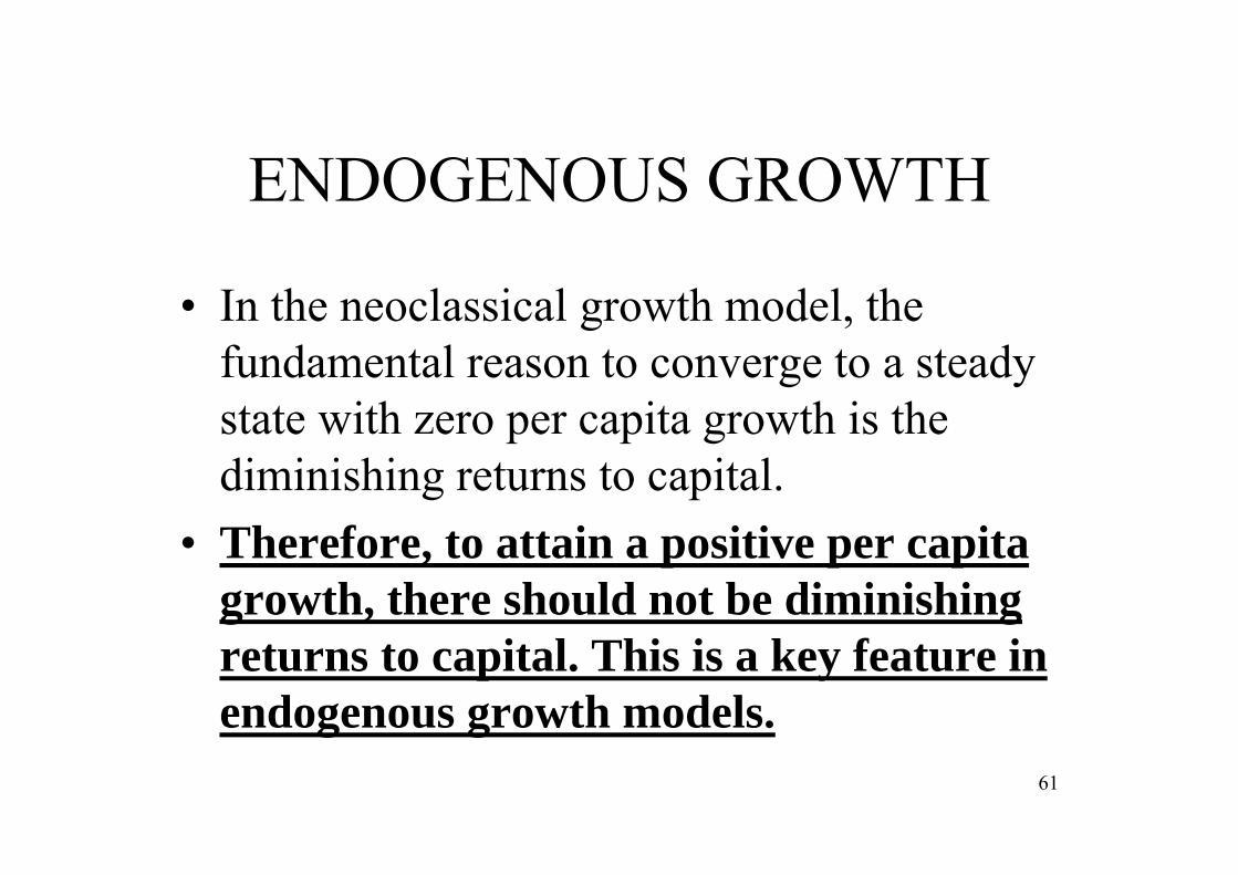
ENDOGENOUS GROWTH
• In the neoclassical growth model, the fundamental reason to converge to a steady state with zero per capita growth is the diminishing returns to capital.
• Therefore, to attain a positive per capita growth, there should not be diminishing returns to capital. This is a key feature in endogenous growth models.
61
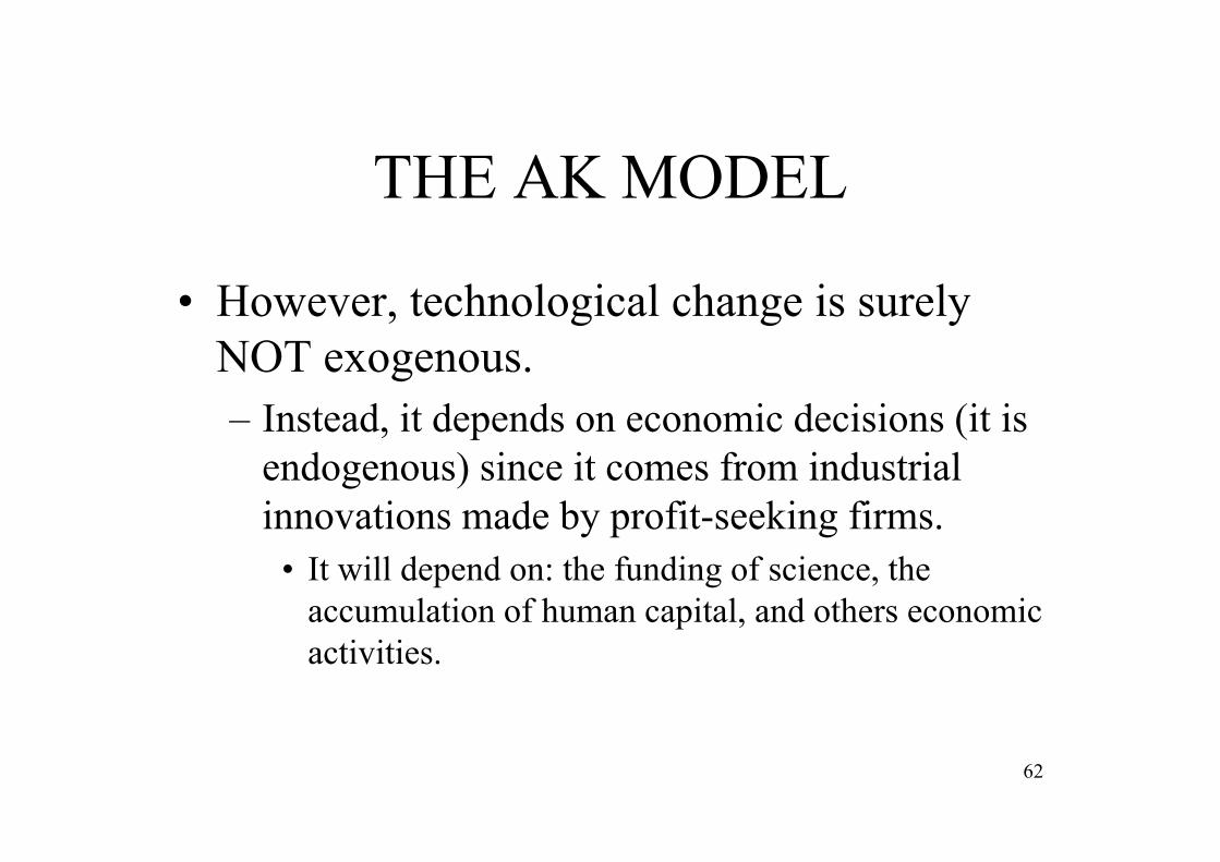
THE AK MODEL
• However, technological change is surely NOT exogenous. – Instead, it depends on economic decisions (it is
endogenous) since it comes from industrial innovations made by profit-seeking firms.
• It will depend on: the funding of science, the accumulation of human capital, and others economic activities.
62

ENDOGENOUS GROWTH
• Incorporating endogenous technology into growth theory forces us to deal with the difficult phenomenon of increasing returns to scale: people must be given an incentive to improve technology.– With constant returns to scale, inputs are paid
according to their marginal products. Then there is nothing to pay for the resources used in improving technology.
– Endogenous theory cannot be based on the usual theory of competitive equilibrium. 63

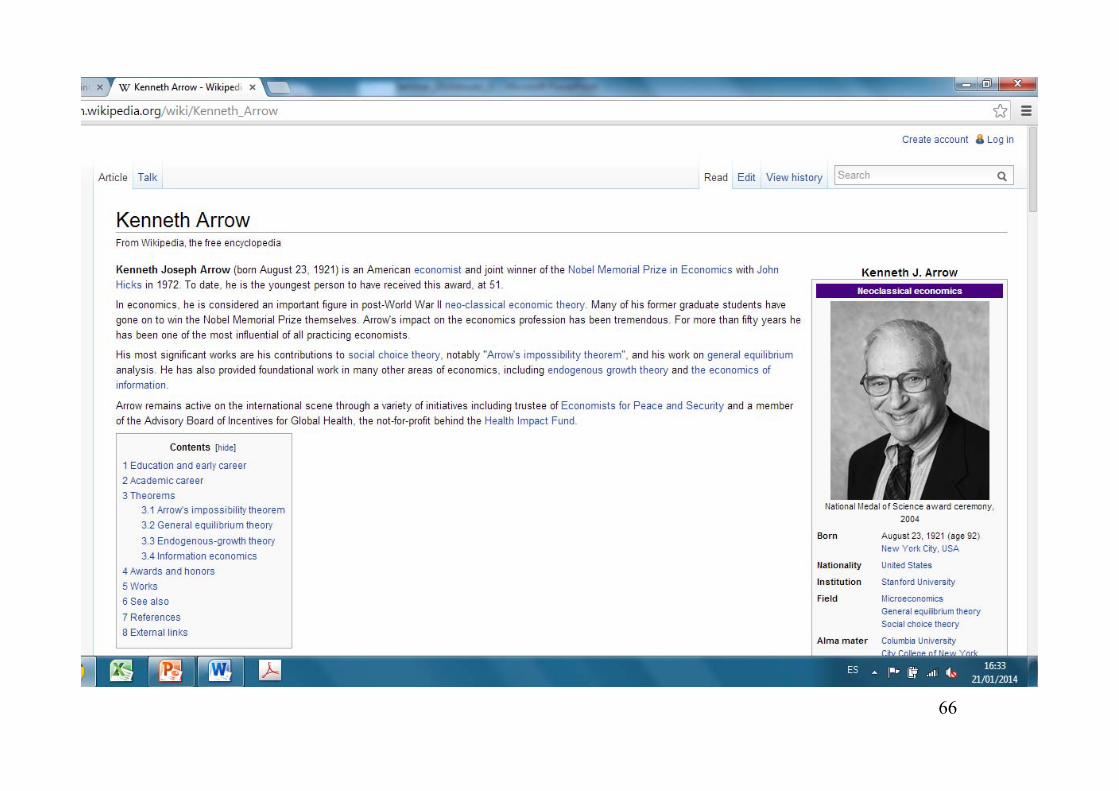
ENDOGENOUS GROWTH• Arrow (1962) proposed a solution:
technological progress is supposed to be an unintended consequence of producing new capital goods, named as “learning by doing” (e.g. airframe manufacturing, shipbuilding, ...). Knowledge creation is a side product of investment. A firm that increases its physical capital learns simultaneously how to produce more efficiently. This positive effect of experience on productivity is called learning by doing (or investing).– Arrow is Nobel Prize winner in Economics 1972.
64
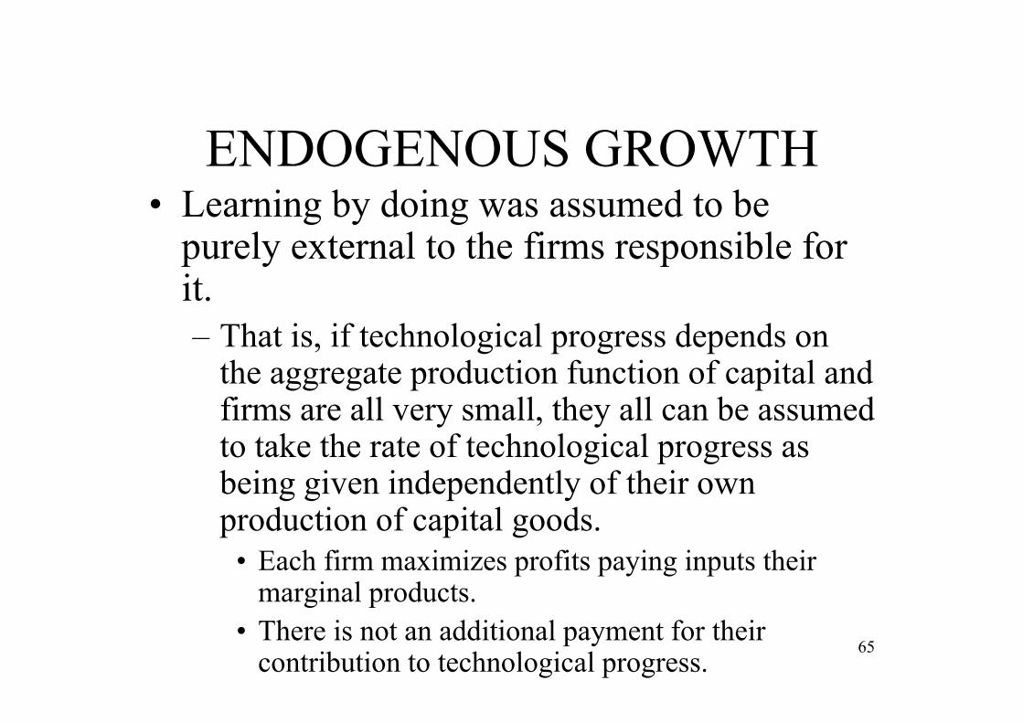
ENDOGENOUS GROWTH• Learning by doing was assumed to be
purely external to the firms responsible for it. – That is, if technological progress depends on
the aggregate production function of capital and firms are all very small, they all can be assumed to take the rate of technological progress as being given independently of their own production of capital goods.
• Each firm maximizes profits paying inputs their marginal products.
• There is not an additional payment for their contribution to technological progress.
65
ENDOGENOUS GROWTH
66
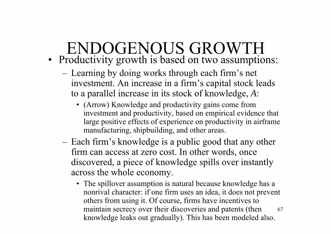
ENDOGENOUS GROWTH• Productivity growth is based on two assumptions:
– Learning by doing works through each firm’s net investment. An increase in a firm’s capital stock leads to a parallel increase in its stock of knowledge, A:
• (Arrow) Knowledge and productivity gains come from investment and productivity, based on empirical evidence that large positive effects of experience on productivity in airframe manufacturing, shipbuilding, and other areas.
– Each firm’s knowledge is a public good that any other firm can access at zero cost. In other words, once discovered, a piece of knowledge spills over instantly across the whole economy.
• The spillover assumption is natural because knowledge has a nonrival character: if one firm uses an idea, it does not prevent others from using it. Of course, firms have incentives to maintain secrecy over their discoveries and patents (then knowledge leaks out gradually). This has been modeled also.
67

THE AK MODEL
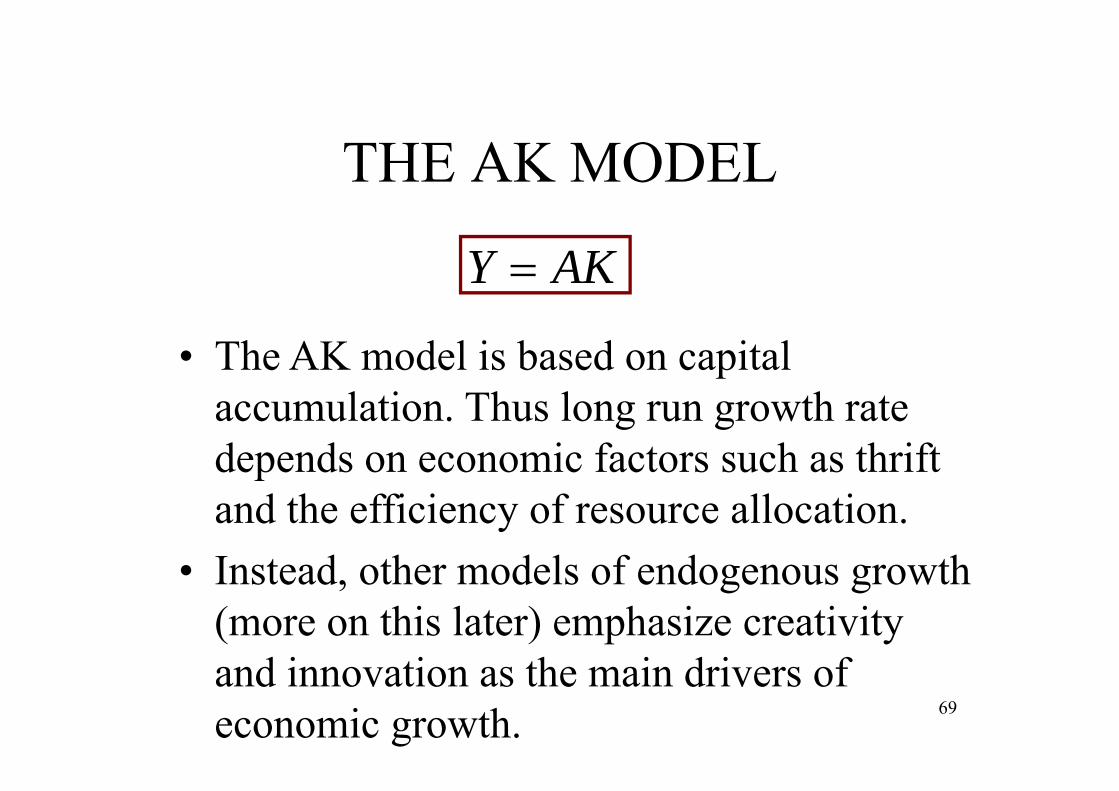
• The AK model assumes that when people accumulate capital, learning by doing generates technological progress that tends to raise the marginal product of capital, thus offsetting the law of diminishing marginal product (when technology is unchanged). Then the marginal product is constant, A:
AKY 68
THE AK MODEL
AKY
• The AK model is based on capital accumulation. Thus long run growth ratedepends on economic factors such as thriftand the efficiency of resource allocation.
• Instead, other models of endogenous growth(more on this later) emphasize creativityand innovation as the main drivers of economic growth. 69

THE HARROD-DOMAR MODEL
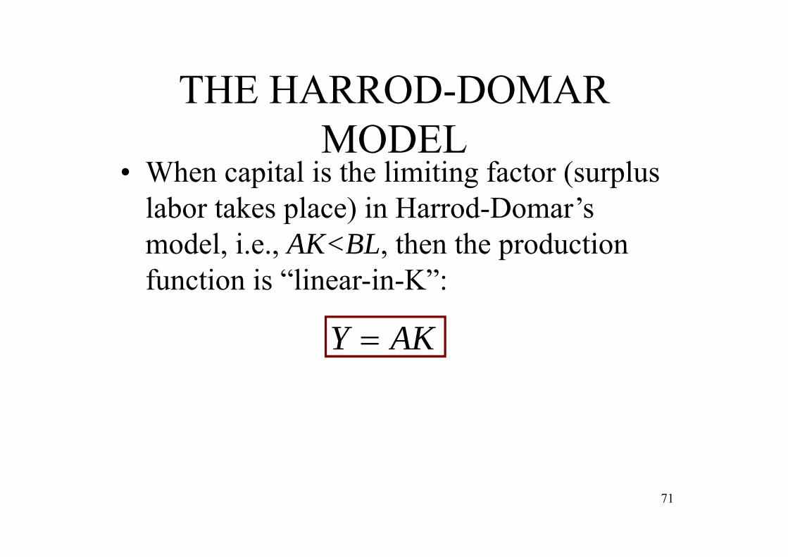
BLAKLKFY ,min),(
• An early precursor of the AK model was that of Harrod-Domar. If the production function has fixed technological coefficients (Leontiev):
• Due to the non-substitutability of inputs, thethere will probably be surplus capital orlabor.
70
THE HARROD-DOMAR MODEL
• When capital is the limiting factor (surplus labor takes place) in Harrod-Domar’smodel, i.e., AK<BL, then the productionfunction is “linear-in-K”:
AKY
71

THE HARROD-DOMAR MODEL
• Then the Solow-Swan equation becomes
• The growth rate of capital will be:tttt KsAKKK 1
sAK
KKgt
tt 1
72
• Since output is linear-in-K, then the rate of growth of output will also be g.
• The growth rate is increasing in the savingsrate s.

THE HARROD-DOMAR MODEL
• The problem with the Harrod-Domar modelis that it cannot explain the sustainedgrowth in output per person exhibited sincethe industrial revolution.• Growth rate of output per worker = g-n• But if this is positive, the growth rate of capital
per worker K/L, g-n, is also positive. • A point will be reached where capital is not the
limiting factor. Then Y=BL, both Y and Lgrowing at the same rate: output per workerceases to grow.
73

NEOCLASSICAL VERSIONOF HARROD-DOMAR
• The first AK model accounting for sustained growth in output per capita is Frankel (1962). His model encompasses:– Solow: perfect competition, substitutability of
factors, and full employment.– Harrod-Domar: long run growth rate depends
on the savings rate.
74

NEOCLASSICAL VERSIONOF HARROD-DOMAR
• The model is based on “Learning by doing”: individual firms contribute to the accumulation of technological knowledge (development) when they accumulate capital (spillover effects: aggregate productivity depends on firms’ specific-sectoral productivity).
1jjj LkAy
N
jjkAA
10
reflects the extent of the knowledge externalities generatedamong firms (if =0 there are not externalities)
75
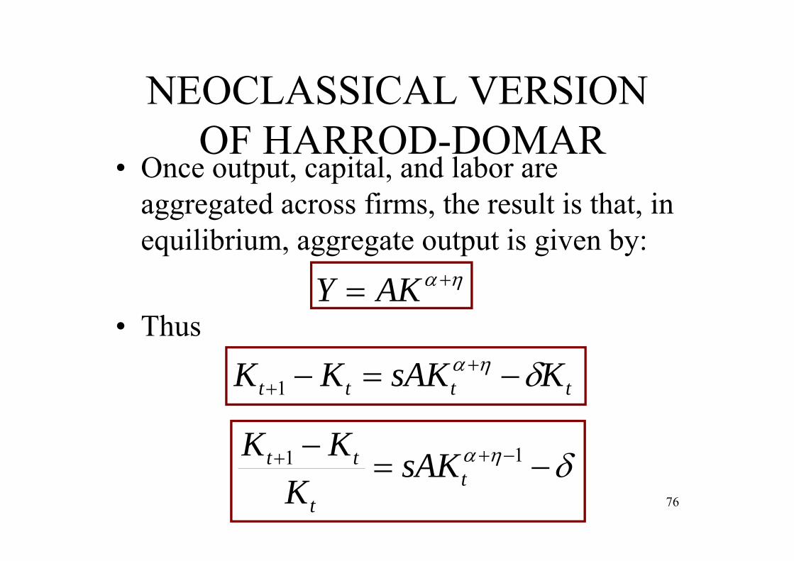
NEOCLASSICAL VERSIONOF HARROD-DOMAR
• Once output, capital, and labor are aggregated across firms, the result is that, in equilibrium, aggregate output is given by:
AKY
tttt KsAKKK 1
• Thus
11
tt
tt sAKK
KK76

NEOCLASSICAL VERSIONOF HARROD-DOMAR
• And the growth rate of capital is given by
11t
t
tt sAKK
KKg
77
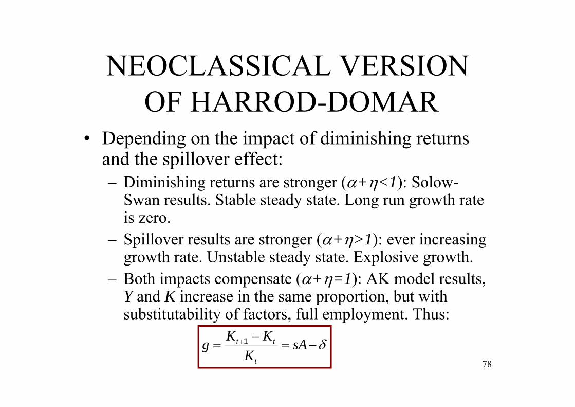
NEOCLASSICAL VERSIONOF HARROD-DOMAR
• Depending on the impact of diminishing returns and the spillover effect: – Diminishing returns are stronger (+<1): Solow-
Swan results. Stable steady state. Long run growth rate is zero.
– Spillover results are stronger (+>1): ever increasing growth rate. Unstable steady state. Explosive growth.
– Both impacts compensate (+=1): AK model results, Y and K increase in the same proportion, but with substitutability of factors, full employment. Thus:
78
sAK
KKgt
tt 1
NEOCLASSICAL VERSIONOF HARROD-DOMAR
• Please note that intertemporal utility maximization can be easily incorporated to the model.
79
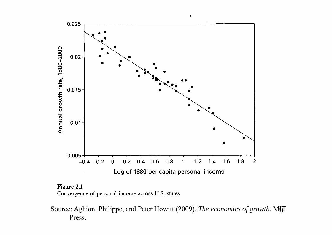
THE AK MODEL
• There is a vast literature on the empirical debate between between neoclassical and AK growth models:– Persistent positive growth rates of per capita GDP in
most countries worldwide. This fact can be explained by the AK growth model, but not by the neoclassical model.
– Cross-country or cross- regional convergence, either absolute (irrespective of their characteristics) or conditional (given similar characteristics). This runs in favor of the neoclassical model. Club convergence.
80
Source: Aghion, Philippe, and Peter Howitt (2009). The economics of growth. MIT Press.
81

THE AK MODEL
• An underlying difficulty for the AK modelis that there is no explicit distinctionbetween capital accumulation and technological progress.
• The next models focus mainly oninnovation-based models that make thatdistinction explicit.
82
3.4: THE PRODUCT VARIETY MODEL
83

THE PRODUCT VARIETY MODEL
• This is the third wave (“second family”) in modern economic growth: innovation-based growth models related to product variety (Romer, 1990).
• Innovation causes productivity growth by creating new, but not necessarily improved, varieties of products.
84

THE PRODUCT VARIETY MODEL
• Productivity comes from an expanding variety of specialized intermediate products. Product variety expands gradually because discovering how to produce a large range of products takes real resources, including time.
• Growth is induced and sustained by increased specialization (A.A. Young, 1928). 85
THE PRODUCT VARIETY MODEL
• For each new product there is a sunk cost of product innovation that must be incurred just once, when the product is first introduced, and never again. The sunk costs can be taken as costs of research, an activity that adds to the stock of technological knowledge.
86

THE PRODUCT VARIETY MODEL
• Technological knowledge consists of a list of blueprints, each of them describing how to produce a different product, and every innovation adds one more blueprint to the list (understood as basic innovation, as if a new industry were opened up). Identifying the state of the technology with the number of varieties should be seen as a metaphor.
87
THE PRODUCT VARIETY MODEL
• Differences with AK model:– Sunk cost of product development, AND– Fixed costs make product markets
monopolistically competitive rather than perfectly competitive. Imperfect competition creates profits, and these profits act as a reward for the creation of new products.
• This allows to “solve” the problem created by Euler’s theorem (given that perfect competition exhausts income). 88

THE PRODUCT VARIETY MODEL
• Elements of the basic model:– Consumers. Utility maximizers.– Firms. Profit maximizers.
• Research sector. Perfect competition. Spending on researchcreates new blueprints (that is, expands the number of varieties). A blueprint has a value for its inventor.
• Producers of intermediate goods, which are different fromeach other. Each interm. good is monopolized by the personwho created the blueprint.
• Producers of final goods. Perfect competition. Intermediategoods are used as inputs. The final good is devoted toconsumption, production of blueprints, and production of interm. goods.
89
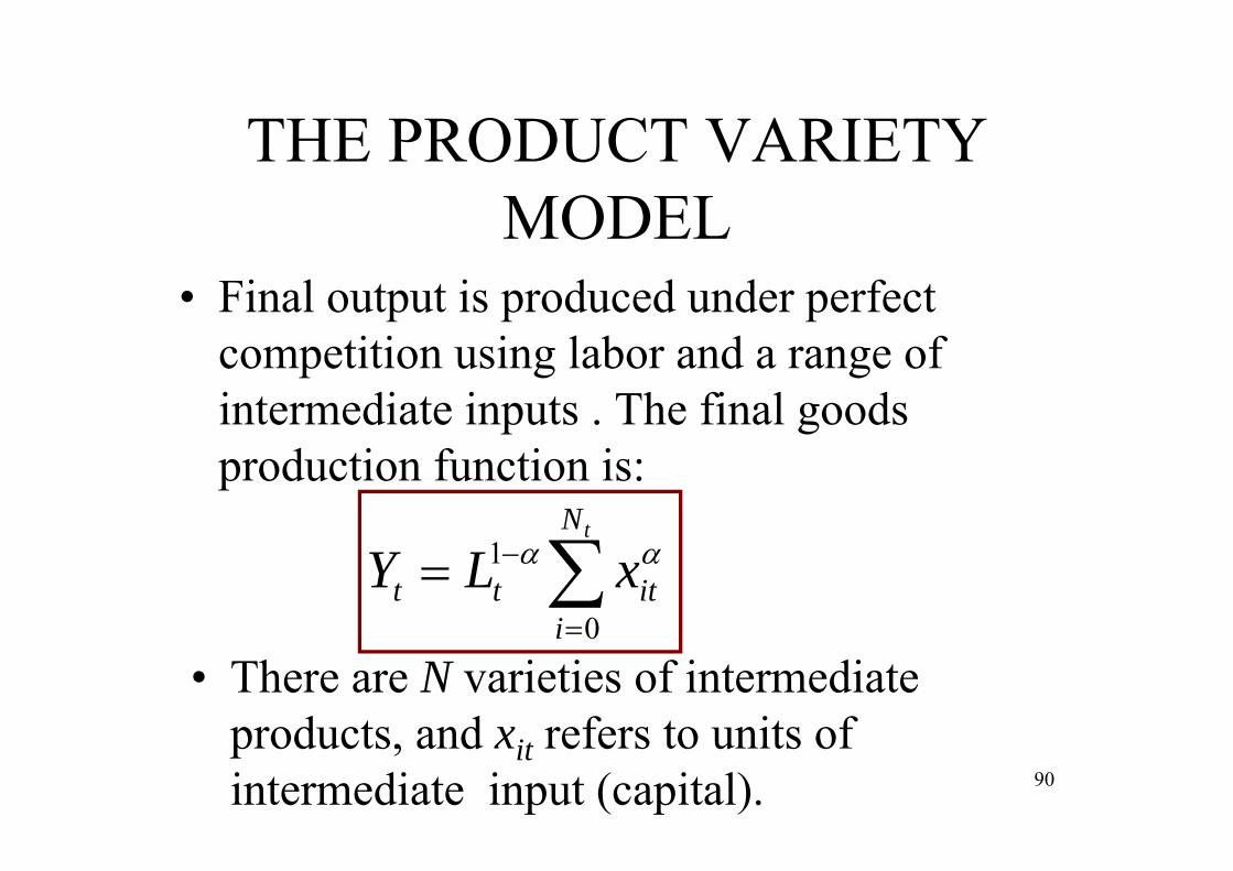
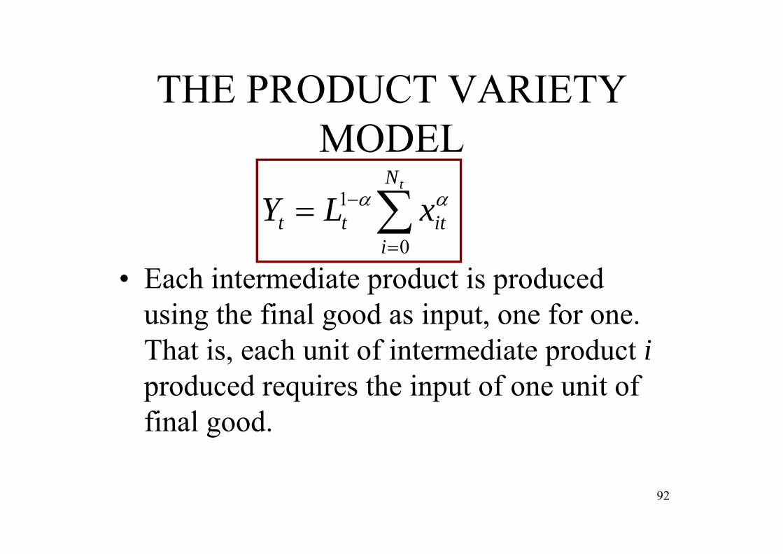
THE PRODUCT VARIETY MODEL
• Final output is produced under perfect competition using labor and a range of intermediate inputs . The final goods production function is:
tN
iittt xLY
0
1
• There are N varieties of intermediateproducts, and xit refers to units of intermediate input (capital). 90

THE PRODUCT VARIETY MODEL
• The production function exhibits diminishing marginal products of each input but constant returns to scale in all inputs together.
• The function is additively separable: marginal products of intermediate goods are independent. New discoveries do not convert others obsolete.
tN
iittt xLY
0
1
91
THE PRODUCT VARIETY MODEL
tN
iittt xLY
0
1
• Each intermediate product is producedusing the final good as input, one for one. That is, each unit of intermediate product iproduced requires the input of one unit of final good.
92
THE PRODUCT VARIETY MODEL
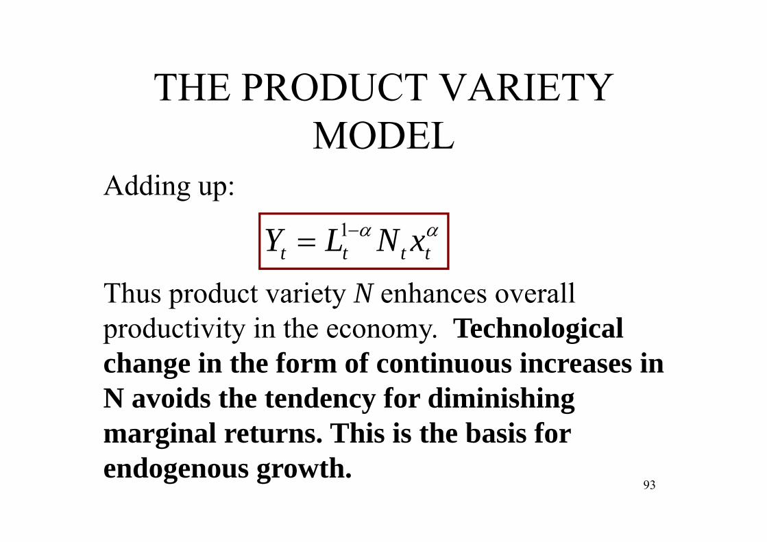
tttt xNLY 1
93
Thus product variety N enhances overall productivity in the economy. Technological change in the form of continuous increases in N avoids the tendency for diminishing marginal returns. This is the basis for endogenous growth.
Adding up:

THE PRODUCT VARIETY MODEL
tN
iit xX
0
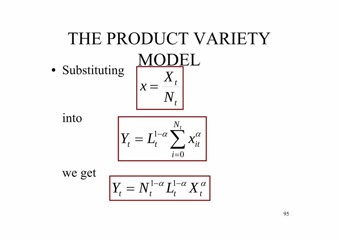
Xt is the total amount of final good used in producingintermediate products.
• Suppose that each intermediate product isproduced in the same amount x (in equilibrium). Then
t
t
NXx
94
By symmetry, aggregate stock of capital Xt is divided into the Ntvarieties evenly.
THE PRODUCT VARIETY MODEL
• Substituting
tttt XLNY 11
95
t
t
NXx
into
tN
iittt xLY
0
1
we get

THE PRODUCT VARIETY MODEL
• Given L, if intermediates Nx expand:– Taking the form of increases in x, diminishing
returns are found.– However, with increases in N diminishing
returns do not arise.• Increasing N encompasses technological
change: diminishing returns do not take place. Endogenous growth occurs. 96
tttttttt xNLNXLNY 1111

THE PRODUCT VARIETY MODEL
• The degree of product variety is the economy’s aggregate productivity parameter, and its growth is the long-run growth rate of per capita worker.
• More product variety raises output potential because a given capital stock is spread over a large number of uses, each of which shows diminishing returns. 97
tttttttt xNLNXLNY 1111

THE PRODUCT VARIETY MODEL
• Increasing product variety sustains growth.• New varieties (new innovations) themselves
result from R&D investments by research-entrepreneurs, who are motivated by the prospect of (perpetual) monopoly rents if they successfully innovate.
• There is only one kind of innovation, which always results in the same kind of new product.
98

THE PRODUCT VARIETY MODEL
• The empirical evidence does not seem to provide a strong support for this model.
• In addition, there is no role for exit and turnover in the economy.
99
3.5: THE SCHUMPETERIAN MODEL
100
101

THE SCHUMPETERIAN MODEL
• This is the third wave (“third family”) in modern economic growth. Again this is an innovation-based growth model, also known as the Schumpeterian model since it involves “creative destruction” (Schumpeter, 1942): quality-improving innovations created by new technologies render old products obsolete (Aghion and Howitt, 1992, 1998).
102
THE SCHUMPETERIAN MODEL
103
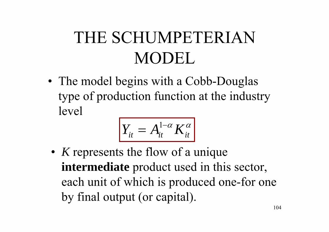
THE SCHUMPETERIAN MODEL
• The model begins with a Cobb-Douglas type of production function at the industry level
ititit KAY 1
104
• K represents the flow of a unique intermediate product used in this sector, each unit of which is produced one-for one by final output (or capital).
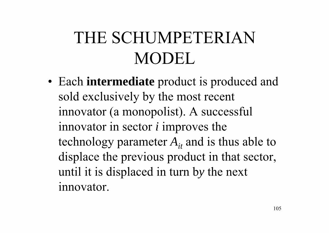
THE SCHUMPETERIAN MODEL
• Each intermediate product is produced and sold exclusively by the most recent innovator (a monopolist). A successful innovator in sector i improves the technology parameter Ait and is thus able to displace the previous product in that sector, until it is displaced in turn by the next innovator.
105
THE SCHUMPETERIAN MODEL
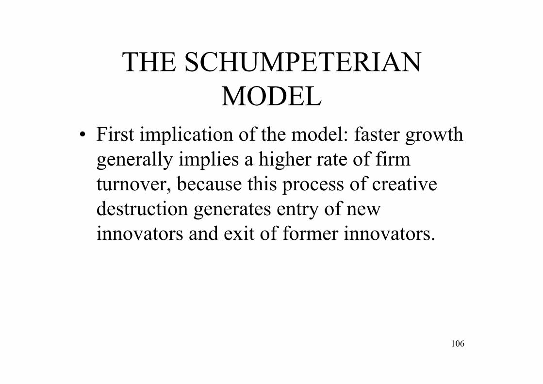
• First implication of the model: faster growth generally implies a higher rate of firm turnover, because this process of creative destruction generates entry of new innovators and exit of former innovators.
106
THE SCHUMPETERIAN MODEL
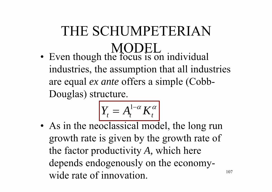
• Even though the focus is on individual industries, the assumption that all industries are equal ex ante offers a simple (Cobb-Douglas) structure.
ttt KAY 1
107
• As in the neoclassical model, the long run growth rate is given by the growth rate of the factor productivity A, which here depends endogenously on the economy-wide rate of innovation.

THE SCHUMPETERIAN MODEL
• There are two main inputs to innovation:– The private expenditures made by the
prospective innovator, and– The stock of innovations that have already been
made by past innovators: publicly available stock of knowledge (current innovators can add to it).
ttt KAY 1
108

THE SCHUMPETERIAN MODEL
– (Cont.) Stock of innovations available:• An innovation that leapfrogs (“salto de rana”) the best
available technology available before the innovation, resulting in a new technology parameter Ait in the innovating sector i, which is some multiple of its preexisting value: LEADING-EDGE INNOVATION.
• An innovation that catches up to a global technology frontier Ât(the stock of global technological knowledge available to innovators in all sectors in all countries). IMPLEMENTING (IMITATING) INNOVATION
ttt KAY 1
109
THE SCHUMPETERIAN MODEL
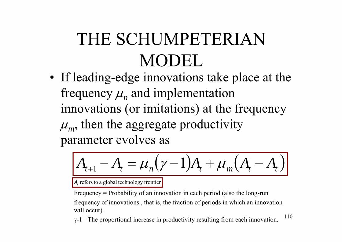
• If leading-edge innovations take place at the frequency n and implementation innovations (or imitations) at the frequency m, then the aggregate productivity parameter evolves as
ttmtntt AAAAA 11
110
Frequency = Probability of an innovation in each period (also the long-run frequency of innovations , that is, the fraction of periods in which an innovation will occur).γ-1= The proportional increase in productivity resulting from each innovation.
frontiery technologglobal a torefers tA
THE SCHUMPETERIAN MODEL
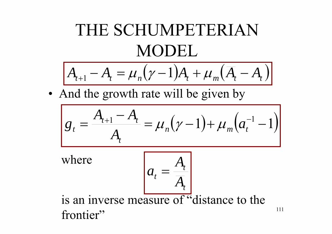
• And the growth rate will be given by
11 11
tmn
t
ttt a
AAAg
ttmtntt AAAAA 11
where
t
tt A
Aa
is an inverse measure of “distance to thefrontier” 111
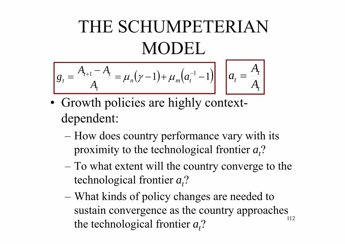
THE SCHUMPETERIAN MODEL
• Growth policies are highly context-dependent:– How does country performance vary with its
proximity to the technological frontier at?– To what extent will the country converge to the
technological frontier at?– What kinds of policy changes are needed to
sustain convergence as the country approaches the technological frontier at?
11 11
tmn
t
ttt a
AAAg
t
tt A
Aa
112
THE SCHUMPETERIAN MODEL
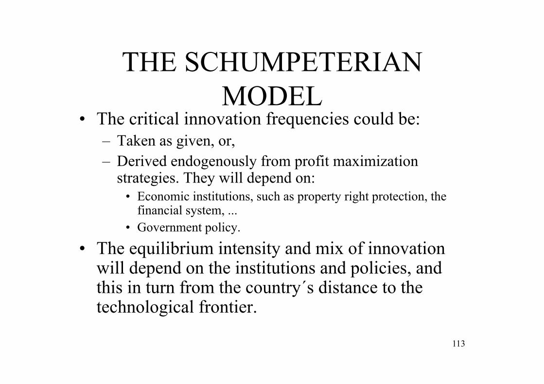
• The critical innovation frequencies could be:– Taken as given, or,– Derived endogenously from profit maximization
strategies. They will depend on:• Economic institutions, such as property right protection, the
financial system, ...• Government policy.
• The equilibrium intensity and mix of innovation will depend on the institutions and policies, and this in turn from the country´s distance to the technological frontier.
113

THE SCHUMPETERIAN MODEL
• This is Gerschenkron´s “advantage from backwardness” (1962): the further the distance, the faster the growth rate, given the frequencies.
• Appropriate institutions can also be easily incorporated in the framework. If institutions favoring imitation are not the same as those favoring leading-edge innovation:– If far from the frontier: imitation. – If close to the frontier: leading-edge innovation.
11 11
tmn
t
ttt a
AAAg
114
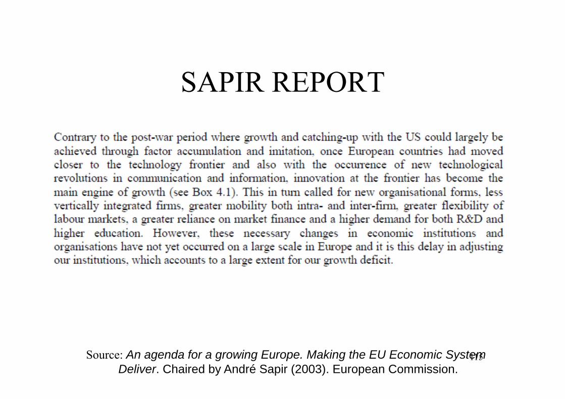
SAPIR REPORT
Source: An agenda for a growing Europe. Making the EU Economic System Deliver. Chaired by André Sapir (2003). European Commission.
115

SAPIR REPORT
Source: An agenda for a growing Europe. Making the EU Economic System Deliver. Chaired by André Sapir (2003). European Commission.
116
TO RECAP: MODELS• First wave: Harrod-Domar (capital accum.).• Second wave: Solow-Swan (capital
accum.).• Third wave:
– First family: AK model (based on capital accumulation).
– Second family: Product variety (innovationbased).
– Third family: Schumpeterian model (innovationbased).
117
4. EMPIRICAL EVIDENCE
118
EMPIRICAL EVIDENCE
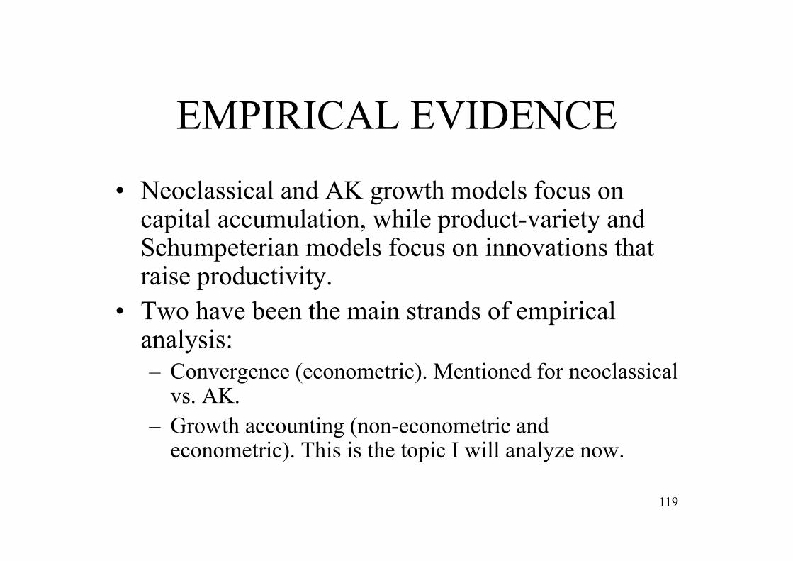
• Neoclassical and AK growth models focus on capital accumulation, while product-variety and Schumpeterian models focus on innovations that raise productivity.
• Two have been the main strands of empirical analysis:– Convergence (econometric). Mentioned for neoclassical
vs. AK.– Growth accounting (non-econometric and
econometric). This is the topic I will analyze now.
119
EMPIRICAL EVIDENCE
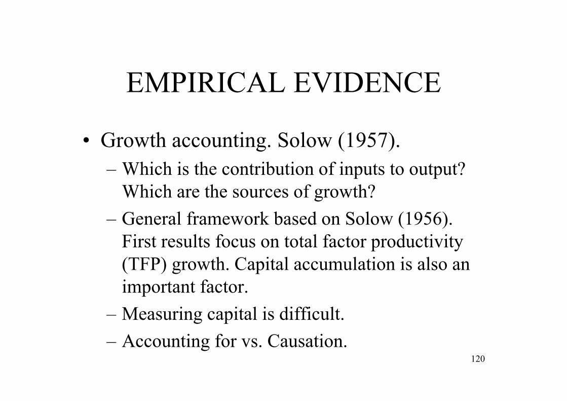
• Growth accounting. Solow (1957). – Which is the contribution of inputs to output?
Which are the sources of growth?– General framework based on Solow (1956).
First results focus on total factor productivity (TFP) growth. Capital accumulation is also an important factor.
– Measuring capital is difficult.– Accounting for vs. Causation.
120

Source: Aghion, Philippe, and Peter Howitt (2009). The economics of growth. MIT Press.
121

EMPIRICAL EVIDENCE
• Directions of new research in growth accounting: – Human capital, – Information and Communication Technologies
capital, and– Intangible assets.
• I will focus on the basic framework in the next section in more detail.
122

5. TWO (PERSONAL) PRACTICAL EXAMPLES
123
TWO (PERSONAL) PRACTICAL EXAMPLES
• Broad recommendation for research: provide a coherent mix of theory and empirical evidence. It makes it much easier to “sell”.
124
5.1: GROWTH ACCOUNTING
125
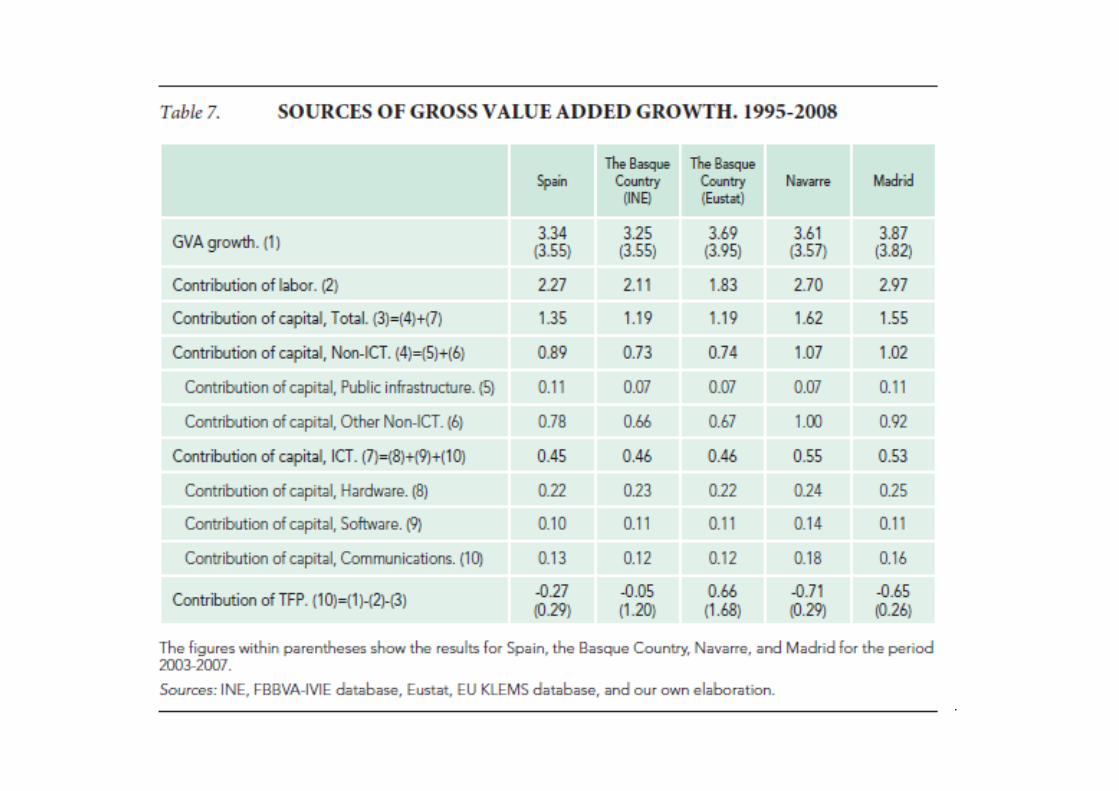
GROWTH ACCOUNTING
• What follows is mostly based on Erauskin(2011): “ACCOUNTING FOR GROWTH IN SPAIN, THE BASQUE COUNTRY (AND ITS THREE HISTORIC TERRITORIES), NAVARRE, AND MADRID SINCE 1965”. – An older paper in 2008 on this issue as well.
126
Introduction
• Motivation:– Post-war period has been a fruitful period as far
as economic progress is concerned.– However, growth did not proceed at a steady
pace.– Territories throughout Spain have performed
unevenly.– Few studies on the whole period 1965-2008.
127
Introduction
• This paper provides a long term analysis on the proximate causes of economic growth for 1965-2008.– Spain, the Basque Country, Navarre, Madrid,
the EU, and the US.
128

The growth accounting methodology
• How does it work? Proximate sources of economic growth (vs. Deep determinants of growth).
• Growth accounting decomposes the growth rate of output into:– Contribution of labor growth.– Contribution of capital growth.– Everything else: “black box”; “measure of our
ignorance”, growth in total factor productivity, …• Origins: Solow (1957).
129
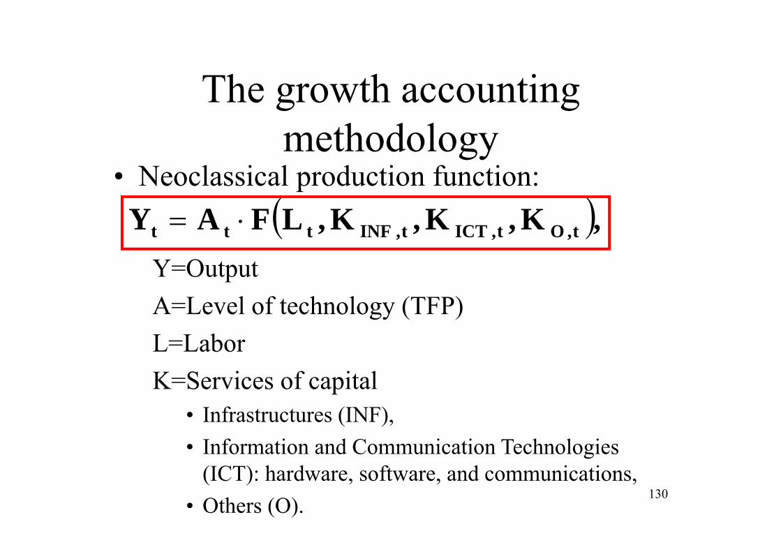
The growth accounting methodology
• Neoclassical production function: ,K,K,K,LFAY t,Ot,ICTt,INFttt
Y=OutputA=Level of technology (TFP)L=LaborK=Services of capital
• Infrastructures (INF),• Information and Communication Technologies
(ICT): hardware, software, and communications, • Others (O).
130
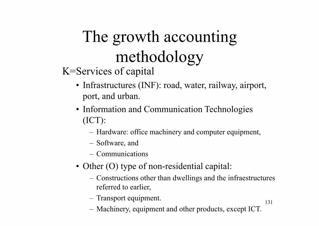
The growth accounting methodology
K=Services of capital• Infrastructures (INF): road, water, railway, airport,
port, and urban.• Information and Communication Technologies
(ICT): – Hardware: office machinery and computer equipment,– Software, and– Communications
• Other (O) type of non-residential capital:– Constructions other than dwellings and the infraestructures
referred to earlier,– Transport equipment.– Machinery, equipment and other products, except ICT.
131
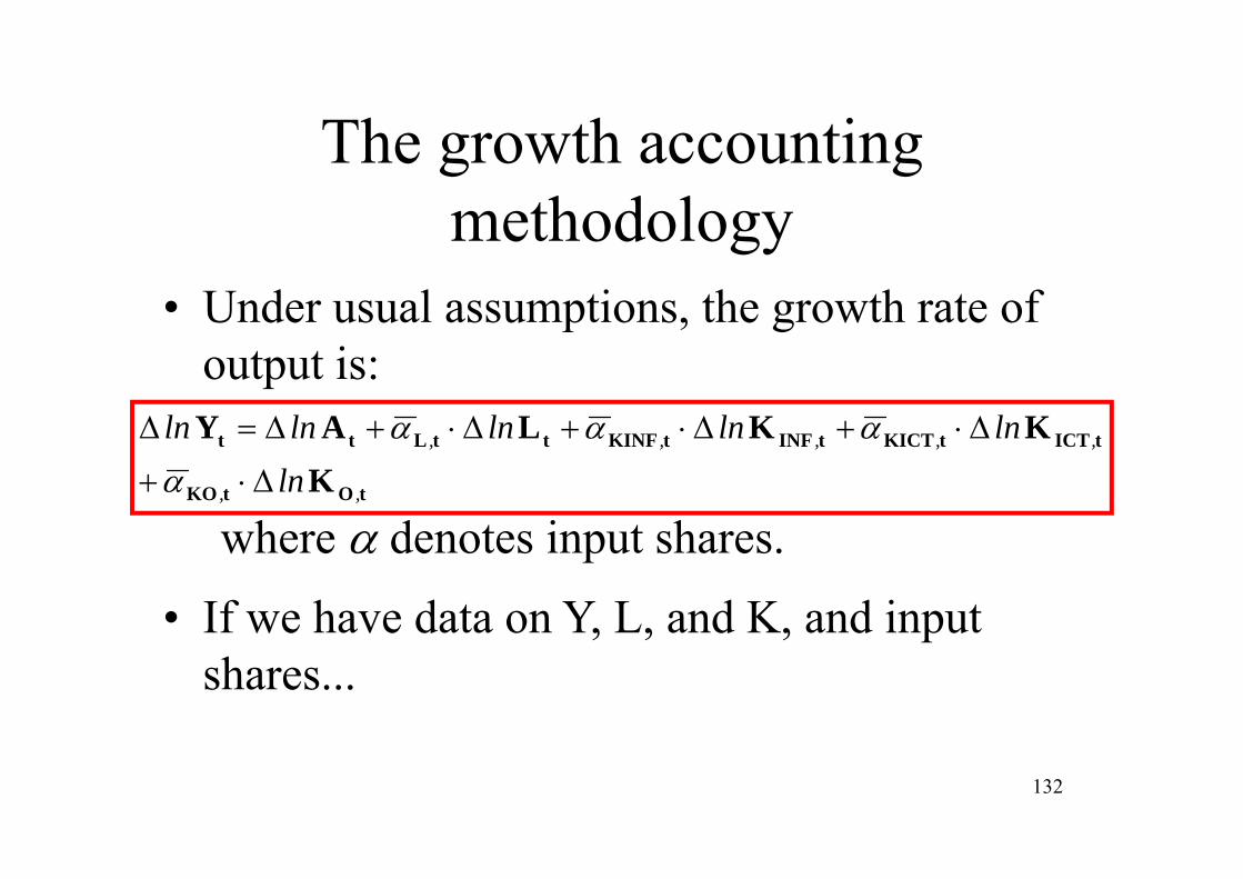
The growth accounting methodology
• Under usual assumptions, the growth rate of output is:
tOtKO
tICTtKICTtINFtKINFttLtt
KKKLAY
,,
,,,,,
lnlnlnlnlnln
where denotes input shares.
• If we have data on Y, L, and K, and input shares...
132

The growth accounting methodology
Then ...
tOtKO
tICTtKICTtINFtKINFttLtt
KKKLYA
,,
,,,,,
lnlnlnlnlnln
= the growth rate of output that cannot beattributed to the (weighted) growth rate of inputs=“Solow residual”=“a measure of ourignorance”=technical innovations, organizational and institutional changes, changes in societal attitudes, fluctuations in demand, changes in factor shares, omittedvariables, and errors of measurement.
133

The growth accounting methodology
• Alternatively:
ttOtKOttICTtKICT
ttINFtKINFttt
LKLKLKALYlnlnlnln
lnlnlnlnln
,,,,
,,
which is very useful to analyze the growth rate of output per hour (or per worker).
134

The growth accounting methodology
• The above equations have been obtained using non-econometric procedures:– They are the most frequently used.– Important advantages over econometric
procedures.
135
Results of previous studies
• Several studies for Spain, but very few for the Autonomous Communities, or provinces in Spain.
• Escriba and Murgui (1998). Growth in TFP and private capital were the sources of growth (1980-1993).
• Gallastegui (2000). Period 1985-1994. 60% was explained by the evolution of private and public capital, employment, training of workers, and expenditure in R+D. 30% was explained by technological change. 136

Results of previous studies
• Goerlich and Mas (2001). Growth in TFP was the main source of growth, followed by private capital (1965-1996).
• Timmer, Ypma and van Ark (2003). 1980-2001– EU: Growth in TFP and capital during 1980-1995.
Increasing contribution of labor during 1995-2001. ICT contribution increased, but not much.
– US: Growth in labor and capital during 1980-1995, and capital and labor during 1995-2001. ICT contribution increased notably.
– Spain: similar sources to those of the EU. Growth in TFP during 1980-1995, and labor during 1995-2001. ICT contribution did not increase.
137
Results of previous studies
• Mas and Quesada (2005). Similar results to those of Timmer et al. (1985-2002).– Labor and capital were the main sources of growth.– The contribution of labor increased enormously, while
that of TFP declined. – Increasing contribution of ICT capital.
• Erauskin (2005). 1986-2000. Private capital and TFP growth fuelled output growth in the Basque Country.
138

Results of previous studies
139

Results of previous studies
140
Results of previous studies• Van Ark, O’Mahony, & Timmer (2008).
– “the European productivity slowdown is attributable to the slower emergence of the knowledge economy in Europe compared to the United States”.
• Lower contribution of ICT capital.• Lower share of technology-producing industry in the
EU.• Lower TFP.
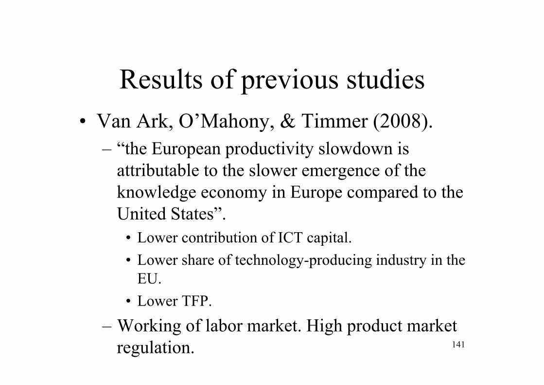
– Working of labor market. High product market regulation. 141
Results of previous studies• Pérez & Robledo (2010). Spain, 1970-2007
– Contribution of capital and labor.– Difference: Declining role of TFP growth.
Causes:• Too much investment in the building sector.• Additional orientation of investment: services.• Deficiencies in education and inadequate working of
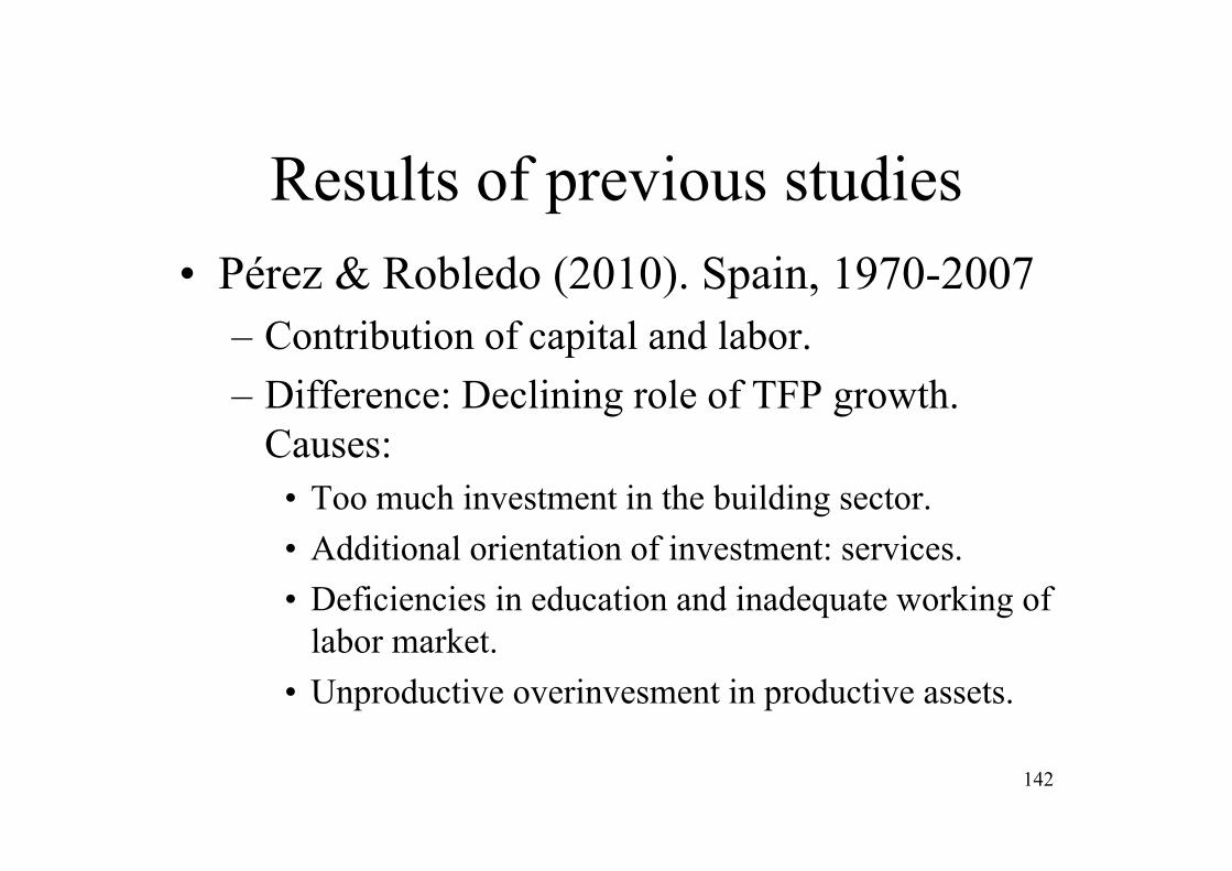
labor market.• Unproductive overinvesment in productive assets.
142
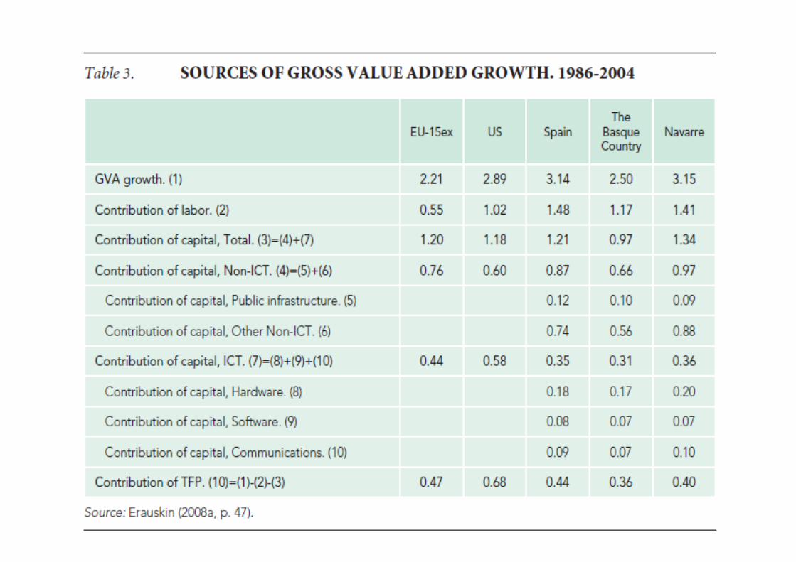
Results of previous studies• Erauskin (2008). Spain, the Basque
Country, and Navarre, 1986-2004.– Higher growth rates for 1995-2004.– Labor and capital growth rates were the main
engines of growth. – TFP growth was residual and it was declining,
even reaching negative figures.
143
Results of previous studies
144
Data sources• Data for the EU and the US: EU KLEMS.
From 1970 (1980) onwards.• Data for Spain:
– National Accounts.• INE.• FBBVA. For data before 1986.
– FBBVA and IVIE: new capital database from 2007 onwards (period 1964-2008).
• Data for the Basque Country (GVA, employment). Independent data from 1980 onwards. 145
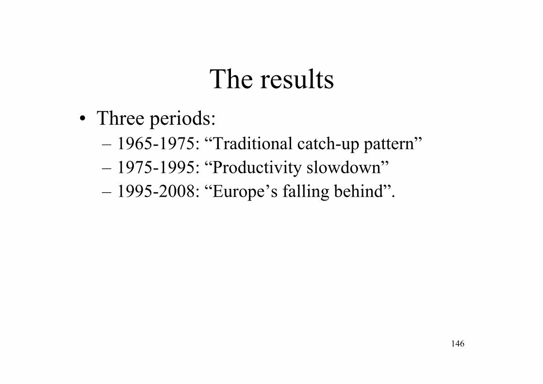
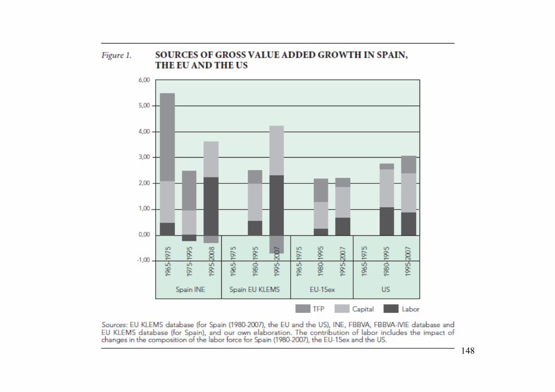
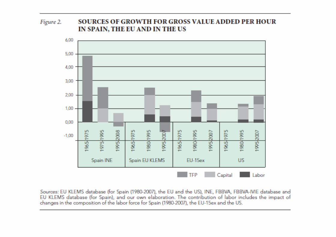
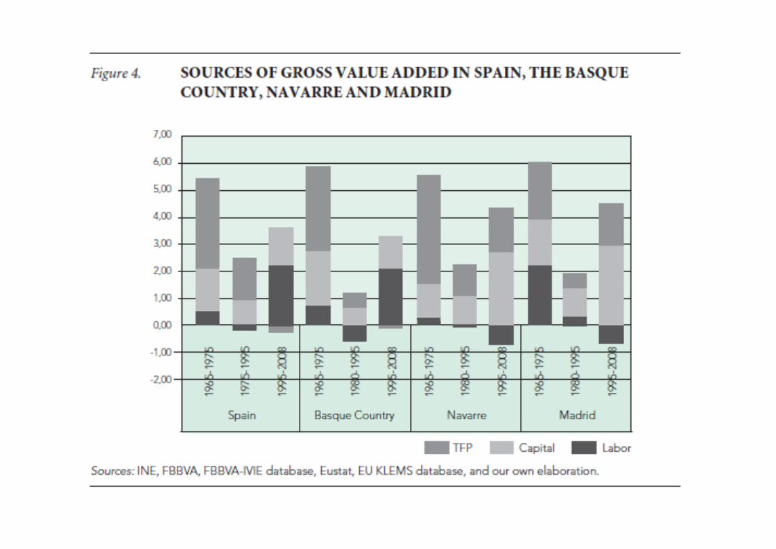
The results• Three periods:
– 1965-1975: “Traditional catch-up pattern”– 1975-1995: “Productivity slowdown”– 1995-2008: “Europe’s falling behind”.
146

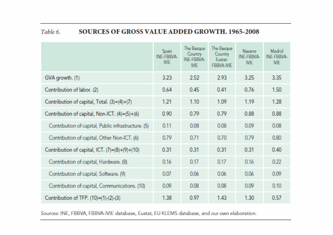
147
148
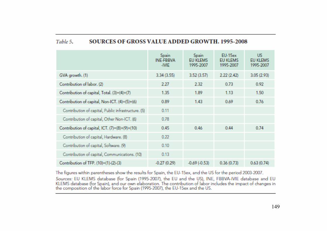
149
150

Different sources of data for the Basque Country
151
152
153
154

Conclusions
1. Growth rates of output.• They were high in the whole period 1965-
2008.2. They were spectacular during 1965-1975.
Sources of economic growth. • Capital and TFP were the main sources of
growth during 1965-2008.• TFP growth played a residual and declining
role in the most recent period 1995-2008.155

Conclusions
3. Some caution on the results for the Basque Country.
• The annual average growth rate of GVA is between 0.25 and 1 % higher if data from Eustat are used, due to differences in GVA deflators (mainly recently) and values in current prices.
156

Conclusions
4. There was an important improvement in the economic performance during 2003-2007, especially for the Basque Country. A “golden-four-year-growth-period”
5. The recent crisis has broken with the expansion period.
157

5.2: CURRENT ACCOUNT BEHAVIOR
158
CURRENT ACCOUNT BEHAVIOR
• Erauskin (2009): “THE CURRENT ACCOUNT AND THE NEW RULE IN A NOT-SO-SMALL OPEN ECONOMY”
159
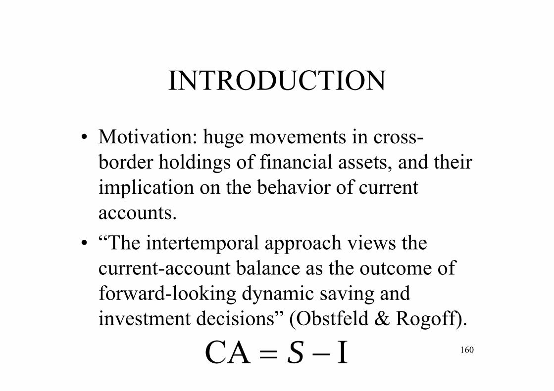
INTRODUCTION
• Motivation: huge movements in cross-border holdings of financial assets, and their implication on the behavior of current accounts.
• “The intertemporal approach views the current-account balance as the outcome of forward-looking dynamic saving and investment decisions” (Obstfeld & Rogoff).
ICA S 160
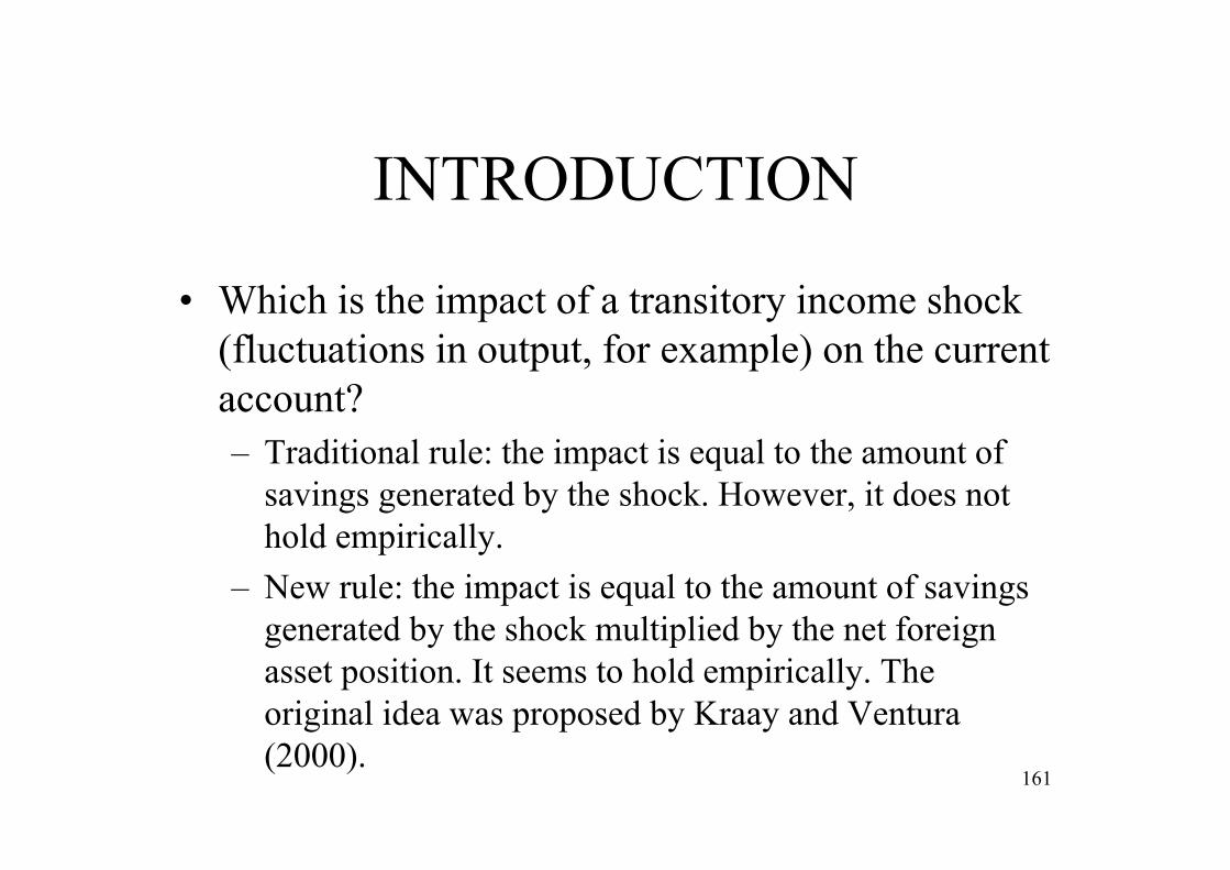
INTRODUCTION
• Which is the impact of a transitory income shock (fluctuations in output, for example) on the current account?– Traditional rule: the impact is equal to the amount of
savings generated by the shock. However, it does not hold empirically.
– New rule: the impact is equal to the amount of savings generated by the shock multiplied by the net foreign asset position. It seems to hold empirically. The original idea was proposed by Kraay and Ventura (2000).
161

INTRODUCTION
• However, it is assumed that the country is a small open economy.
• Contribution of the paper:– Extending the new rule to a not-so-small open
economy: which is the impact of transitory income shocks on the current account in a not-so-small open economy (i.e. in a two-country world)?
– Empirically test the main predictions: how does the theory fit with the empirical data? 162

THEORY
• Endogenous growth: domestic and foreign capital is subject to diminishing returns to capital. Aggregate capital stock has an external effect on labor productivity, but the firm faces decreasing returns to capital. – “We motivate diminishing returns to domestic capital
bluntly as the result of congestion effects or negative externalities. Since the representative consumer is infinitesimal, he/she understands that his/her actions have no influence on the aggregate stock of capital.” (Kraay and Ventura, 2000). 163
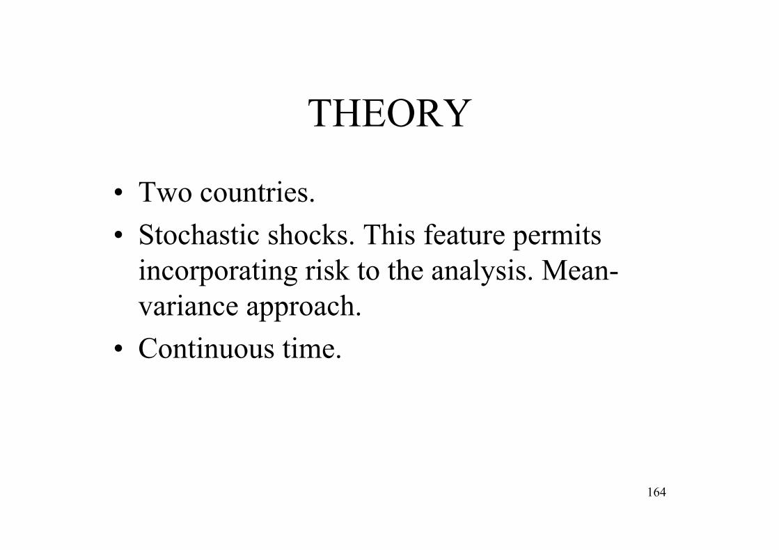
THEORY
• Two countries.• Stochastic shocks. This feature permits
incorporating risk to the analysis. Mean-variance approach.
• Continuous time.
164
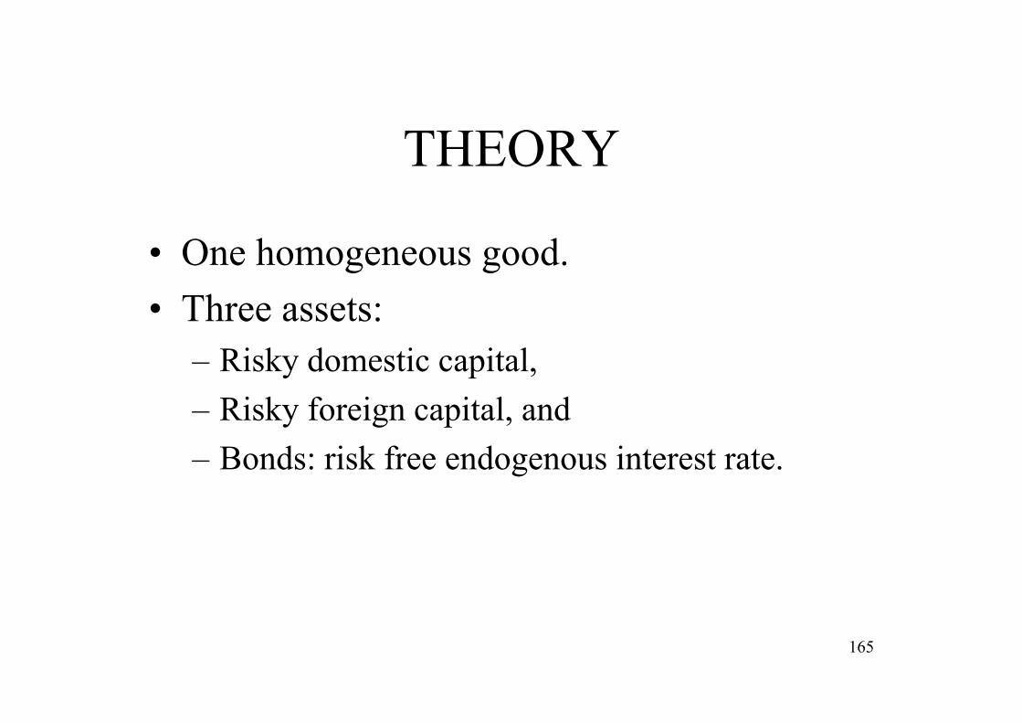
THEORY
• One homogeneous good.• Three assets:
– Risky domestic capital,– Risky foreign capital, and– Bonds: risk free endogenous interest rate.
165

THEORY
BKKW
BKKW
ff
dd
**
*• Domestic and foreign wealth:
166
• Domestic wealth:• Domestic capital in the hands of the domestic economy.• Foreign capital in the hands of the domestic economy.• Net position of risk-free loans.
• Foreign wealth:• Domestic capital in the hands of the foreign economy.• Foreign capital in the hands of the foreign economy.

THEORY• Net foreign asset position:
BKKP fd *
• The current account is equal the variation in its net foreign asset position:
dBdKdKdPCA fd *
167

THEORY
• The current account balance is equal to the variation in domestic wealth (that is, savings ) minus the variation in domestic capital (domestic net investment).
**
WK
dWWKdWdWdKdWISCA fd
168
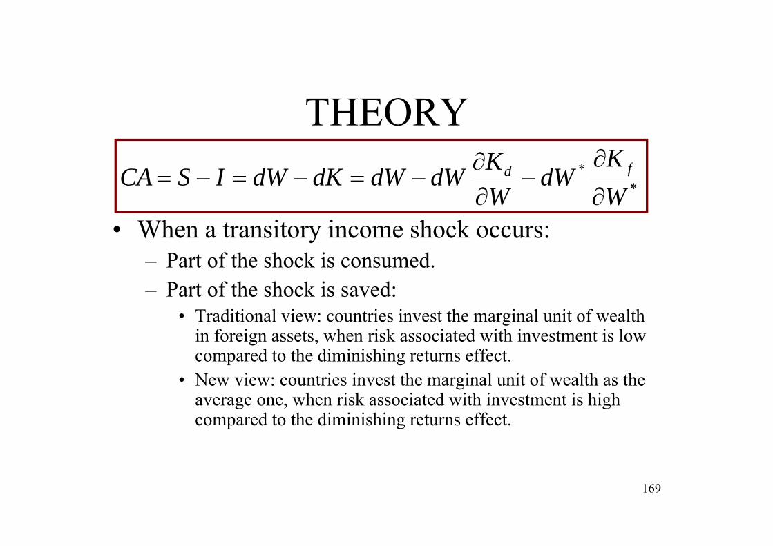
THEORY
• When a transitory income shock occurs:– Part of the shock is consumed.– Part of the shock is saved:
• Traditional view: countries invest the marginal unit of wealth in foreign assets, when risk associated with investment is low compared to the diminishing returns effect.
• New view: countries invest the marginal unit of wealth as the average one, when risk associated with investment is high compared to the diminishing returns effect.
**
WK
dWWKdWdWdKdWISCA fd
169

THEORY: The three results
**
WK
dWWKdWdWCA fd
1) Traditional view: 0
WKd
2) New view:WK
WK dd
0fdK• Small open economy:
3) Not-so-small open economy: ** WK
WK ff
170

TRADITIONAL RULE
dWCA
• Traditional view: 0
WKd
• Result: the impact of transitory income shocks on the current account is equal to the saving generated by the shock.
• Small open economy: 0fdK
171

NEW RULE
WBKdW
WKdWdWCA dd
*
• New view: WK
dWdK dd
• Result: the impact of transitory income shocks on the current account is equal to the saving generated by the shock multiplied by the net foreign asset position of the country.
• Small open economy: 0fdK
172
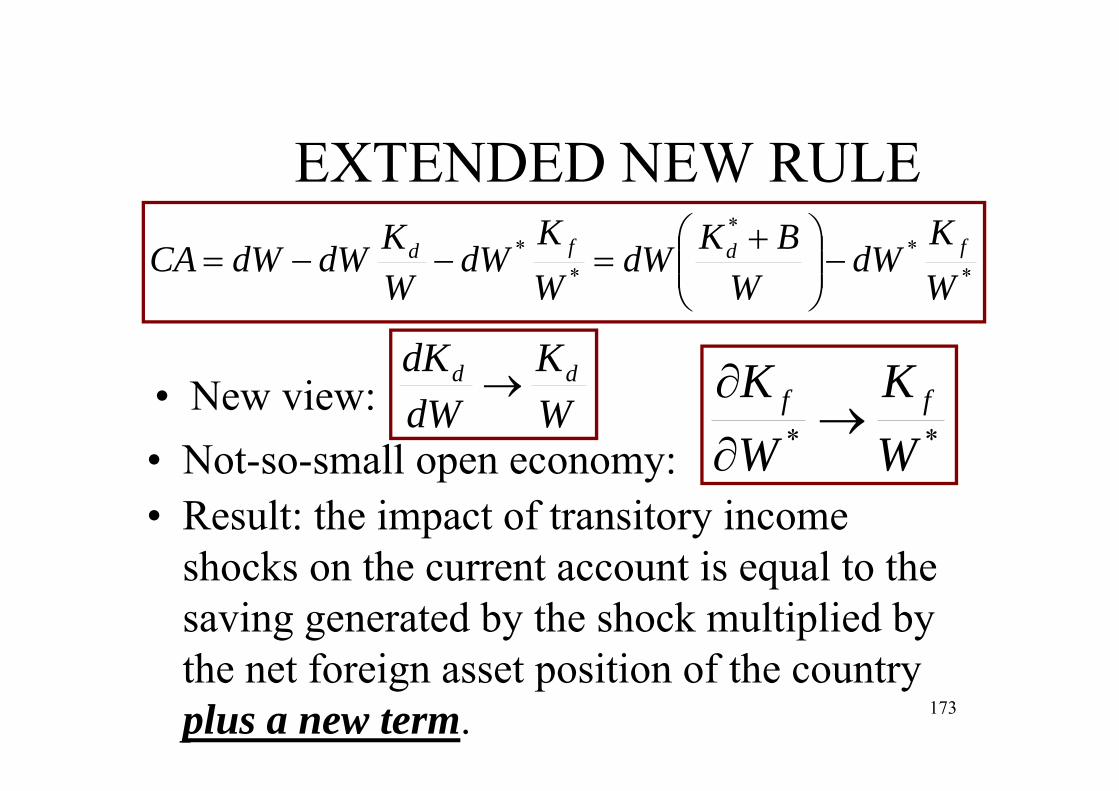
EXTENDED NEW RULE
**
*
**
WK
dWW
BKdWWK
dWWKdWdWCA fdfd
• New view: WK
dWdK dd
** WK
WK ff
• Not-so-small open economy:• Result: the impact of transitory income
shocks on the current account is equal to the saving generated by the shock multiplied by the net foreign asset position of the country plus a new term. 173

DATA SOURCES
• Complex issue• Sample: 19 OECD countries (1970-2004).• The data are based on:
– International Monetary Funds´s International Financial Statistics
– World Bank´s World Development Indicators, and
– Lane and Milesi-Ferretti (2007).174
EMPIRICAL EVIDENCE
175
EMPIRICAL EVIDENCE
176
EMPIRICAL EVIDENCE
177

EMPIRICAL EVIDENCE
178
EMPIRICAL EVIDENCE
179

EMPIRICAL EVIDENCE
180
CONCLUSIONS
• Increasing financial integration has important implications for the current account.
• The traditional rule has failed to account for the empirical evidence on current accounts.
• KV provided an insightful departure from the traditional rule: the new rule. Moreover, the empirical evidence seemed to validate the new rule. However, it is based on a small open economy assumption. 181
CONCLUSIONS
• The paper has suggested an extension to the new rule rule abandoning the small open economy assumption. It is broadly supported by the empirical evidence, which seems to reject the new rule.
182

CURRENT ACCOUNT BEHAVIOR
• Erauskin (2015): “SAVINGS, THE SIZE OF THE NET FOREIGN ASSET POSITION AND THE DYNAMICS OF CURRENT ACCOUNTS”.
MOTIVATION
• Big current account imbalances in recentyears.
• Huge variations in gross and net international investment positions.– Consequences for current accounts are
straightforward.

INTRODUCTION
“The intertemporal approach views thecurrent-account balance as the outcome of forward-looking dynamic saving and investment decisions”.
ICA S
INTRODUCTION
• Which is the impact of a transitory income shock (fluctuations in output, for example) on the current account? There are two main views: – Traditional rule (standard benchmark model):
• This view is appropriate when domestic capital is subject to diminishing returns and risk associated to investment is low.
• The marginal unit of wealth (savings) is invested in foreign bonds.
– Then the impact on the current account is equal to the amount of savings generated by the shock.
• However, the traditional rule does not hold empirically. Feldstein-Horioka puzzle. 186
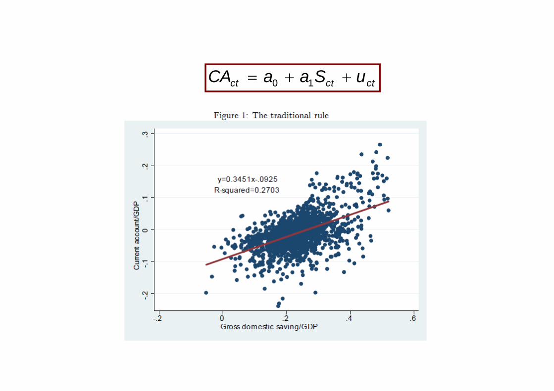
ctctct uSaaCA 10
INTRODUCTION
• Two main views (cont.):– New rule:
• The original idea was proposed by Kraay and Ventura (2000).• This view is appropriate when risk associated to investment is
high compared to the diminishing returns effect. • The marginal unit of wealth (savings) is invested as the
average unit of wealth.• Please note:
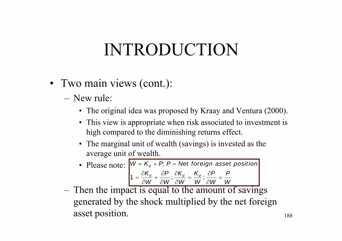
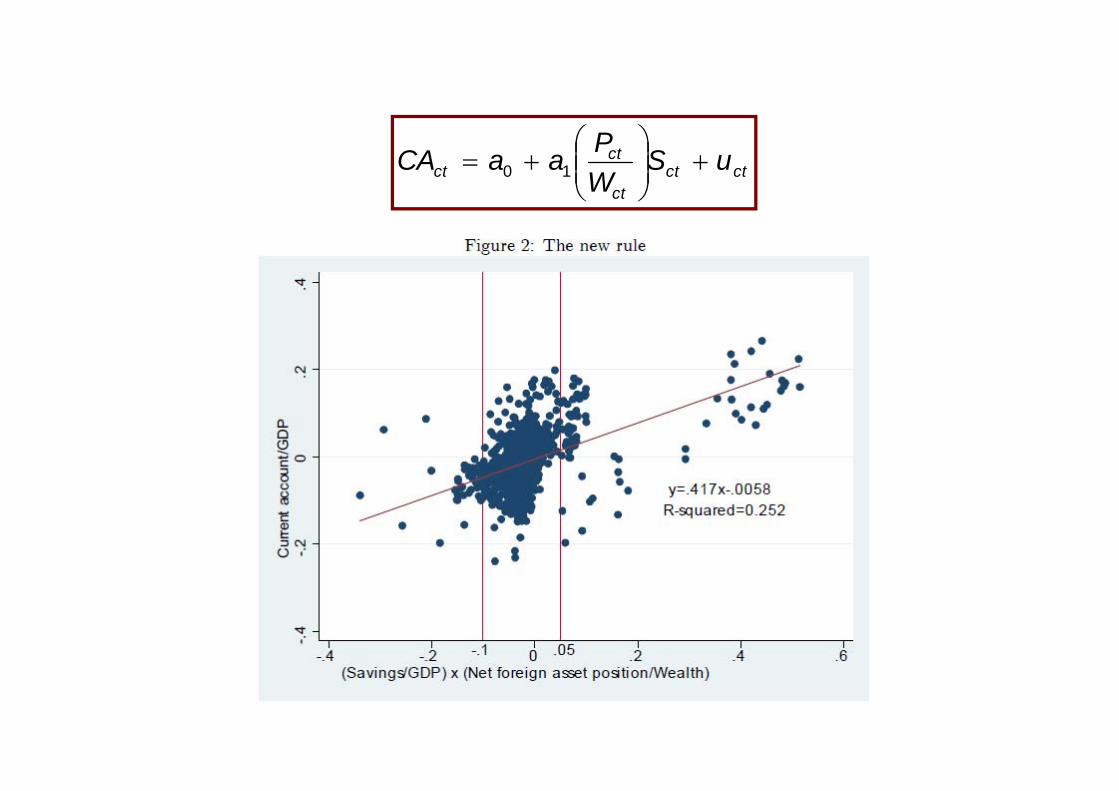
– Then the impact is equal to the amount of savings generated by the shock multiplied by the net foreign asset position. 188
WP
WP
WK
WK
WP
WK
onset positiforeign asNetPPKW
ddd
d
;;1
;
ctctct
ctct uS
WPaaCA
10
INTRODUCTION• This paper offers three main contributions:
– We adapt the new rule to distinguish between gross and net foreign asset positions, because both matter.
– We combine both the new view and the traditional rule.– The empirical evidence suggests that the support for the
traditional rule or the new view depends crucially on the size of the net foreign asset position.
• Intermediate case: the new view dominates.• “Big” creditor (+15% domestic wealth) case: the traditional
rule dominates.• “Big” debtor case (-15% wealth) case: the traditional rule
dominates, but the impact is much weaker than for creditors. 190
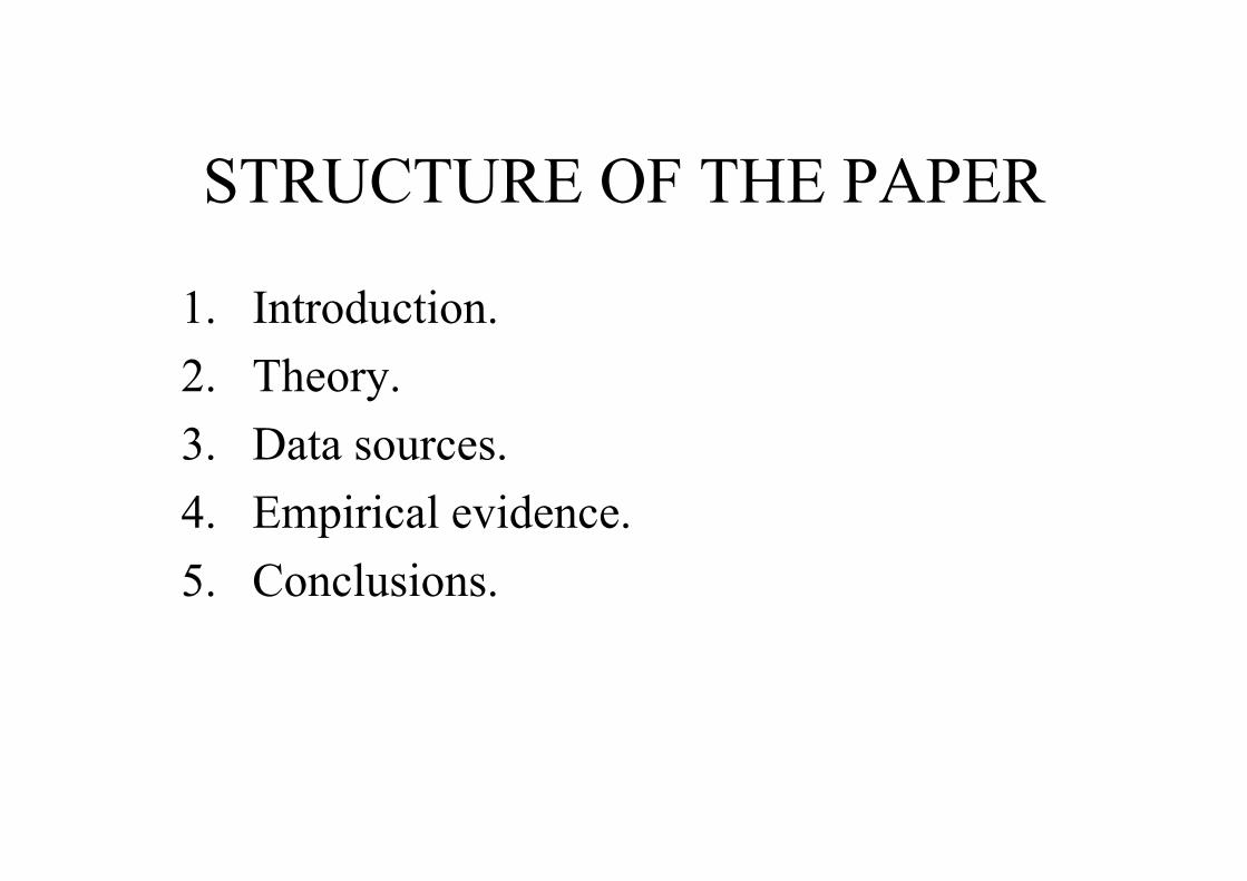
STRUCTURE OF THE PAPER
1. Introduction.2. Theory.3. Data sources.4. Empirical evidence.5. Conclusions.
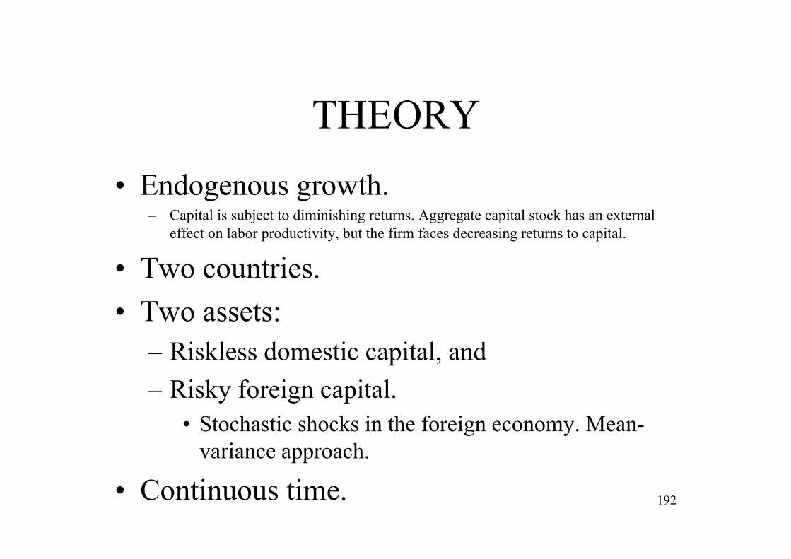
THEORY• Endogenous growth.
– Capital is subject to diminishing returns. Aggregate capital stock has an external effect on labor productivity, but the firm faces decreasing returns to capital.
• Two countries.• Two assets:
– Riskless domestic capital, and– Risky foreign capital.
• Stochastic shocks in the foreign economy. Mean-variance approach.
• Continuous time. 192
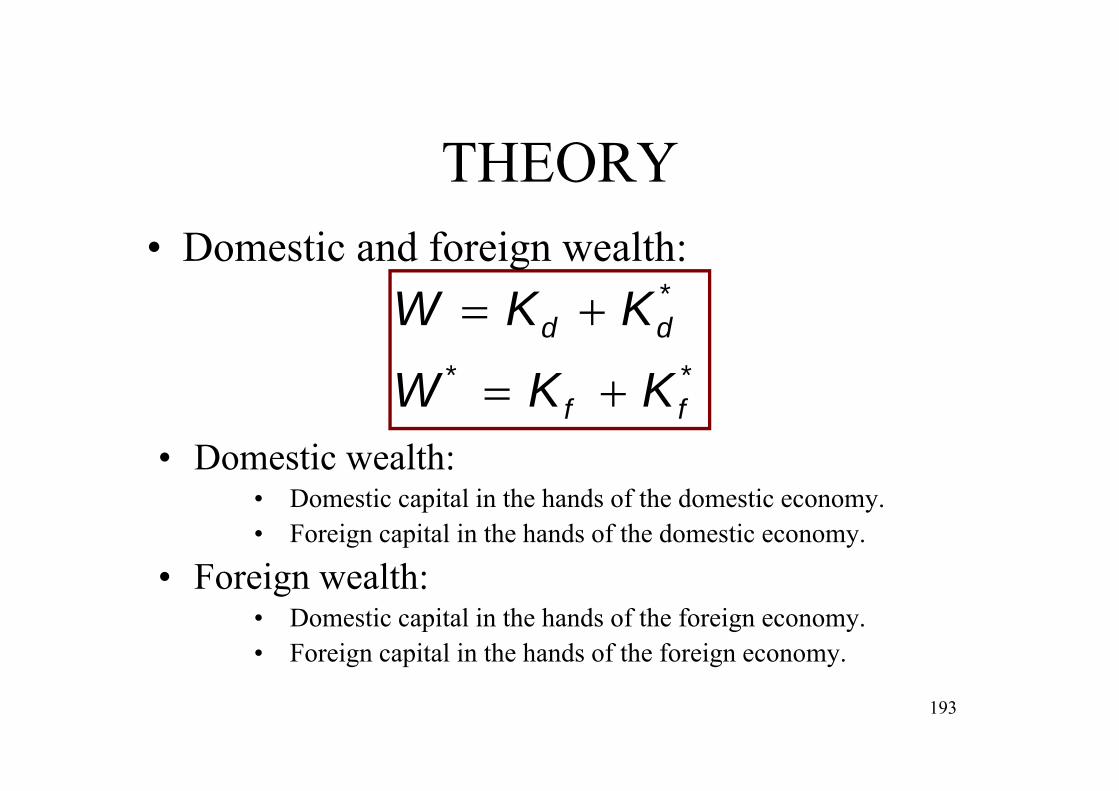
THEORY
**
*
ff
dd
KKWKKW
• Domestic and foreign wealth:
193
• Domestic wealth:• Domestic capital in the hands of the domestic economy.• Foreign capital in the hands of the domestic economy.
• Foreign wealth:• Domestic capital in the hands of the foreign economy.• Foreign capital in the hands of the foreign economy.

THEORY
,;0,;1 0 11
11
0
CdteCEMax t
• Preferences (Stone-Geary):
194
subject to:
dtCdyKdtKKdW ddd*****

THEORY
1/12
*
*
WWK
y
d
• Solution for the domestic economy:
195
2
2*
2
2*
*
*
15.0
115.0
y
y
WC
• Analogous for the foreign economy.

THEORY• Net foreign asset position:
fd KKP *
• The current account is equal the variation in its net foreign asset position (savings minusinvestment):
**
* 1 dWWKdW
WKdKdKdPCA fd
fd
196

THEORY
w
K
WKWK d
y
d
d
2*
/1
1
197
• How do countries react?
2*
/
y
dK
is key.
– If big, – If small,
0WKd
w
KWK dd

THEORY
**
WKdW
WKdWdWCA fd
WK
WK dd
Then:
198
** WK
WK ff
**
*
1 dWWKdW
WKdWCA fd
• How do countries react?
10
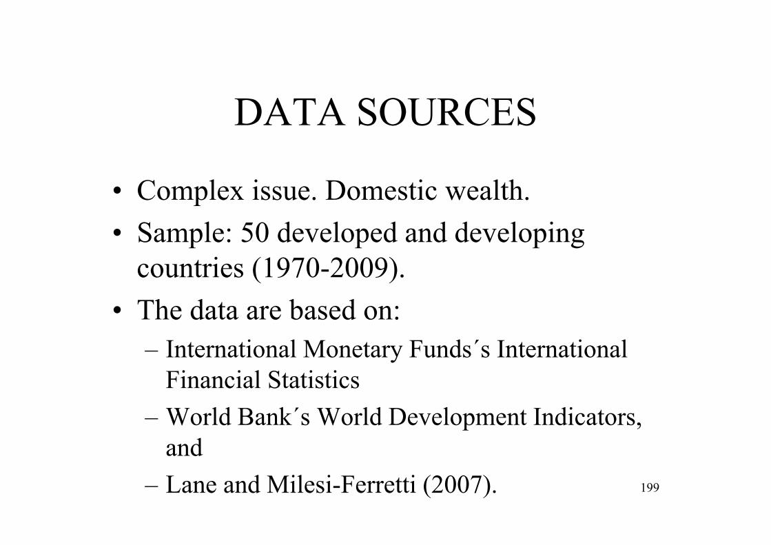
DATA SOURCES
• Complex issue. Domestic wealth.• Sample: 50 developed and developing
countries (1970-2009).• The data are based on:
– International Monetary Funds´s International Financial Statistics
– World Bank´s World Development Indicators, and
– Lane and Milesi-Ferretti (2007). 199
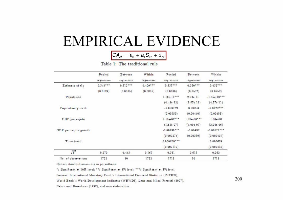
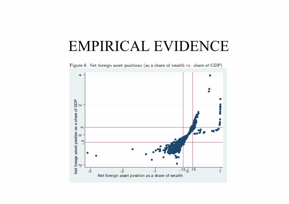
EMPIRICAL EVIDENCE
200
ctctct uSaaCA 10

EMPIRICAL EVIDENCE
201
ctctct
ctct uS
WPaaCA
10

EMPIRICAL EVIDENCE
202
EMPIRICAL EVIDENCE
203
ctctct
ctct uS
WPaaCA
10
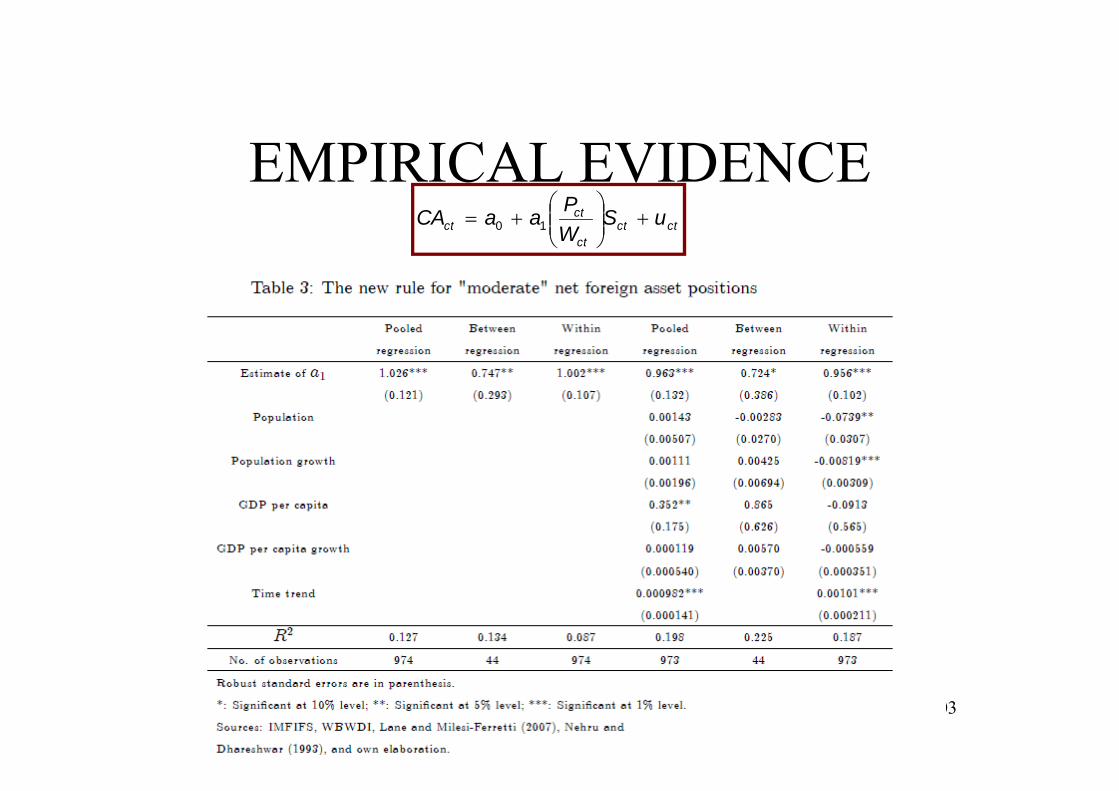
EMPIRICAL EVIDENCE

EMPIRICAL EVIDENCE
205
ctctct
ctct uS
WPaaCA
10
EMPIRICAL EVIDENCE
206
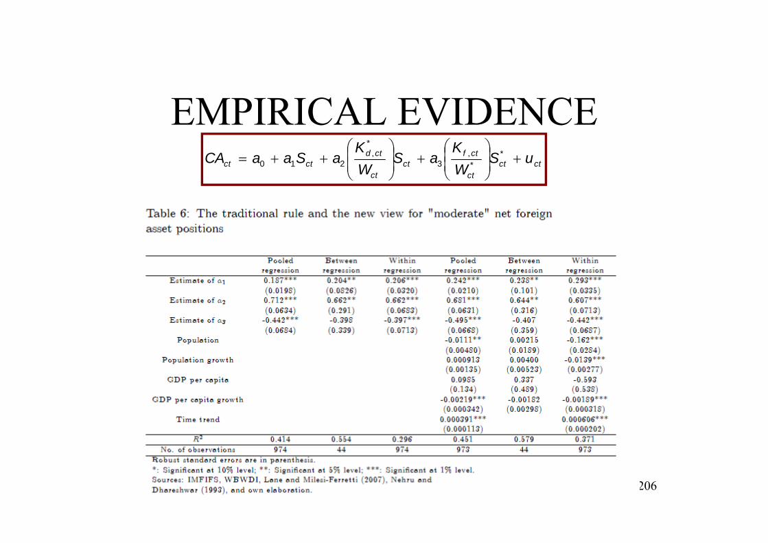
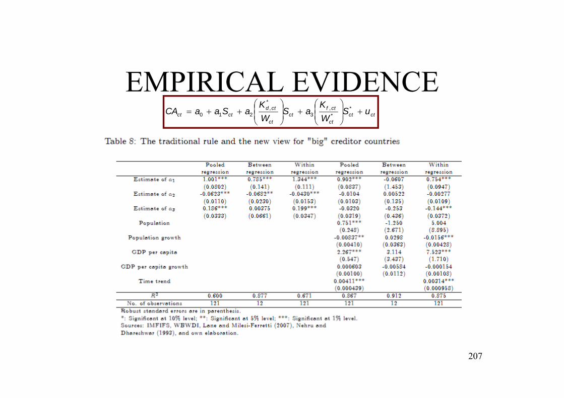
ctctct
ctfct
ct
ctdctct uS
WK
aSWK
aSaaCA
*
*,
3
*,
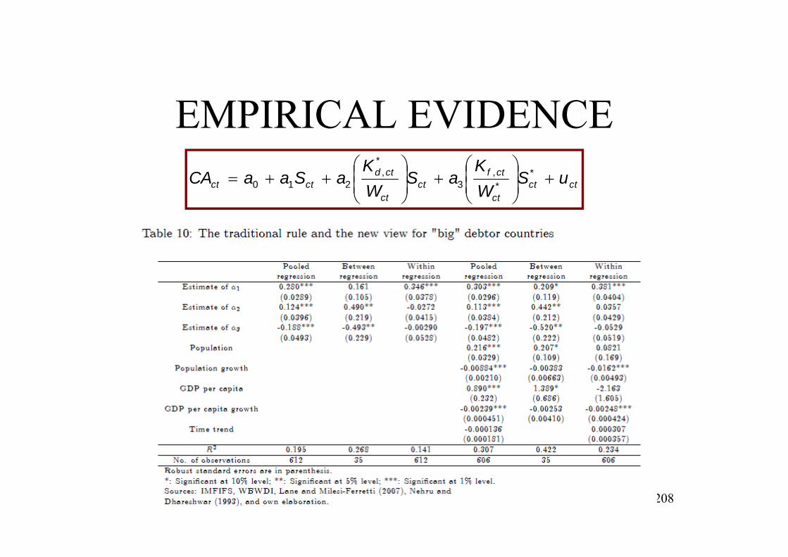
210
EMPIRICAL EVIDENCE
207
ctctct
ctfct
ct
ctdctct uS
WK
aSWK
aSaaCA
*
*,
3
*,
210
EMPIRICAL EVIDENCE
208
ctctct
ctfct
ct
ctdctct uS
WK
aSWK
aSaaCA
*
*,
3
*,
210
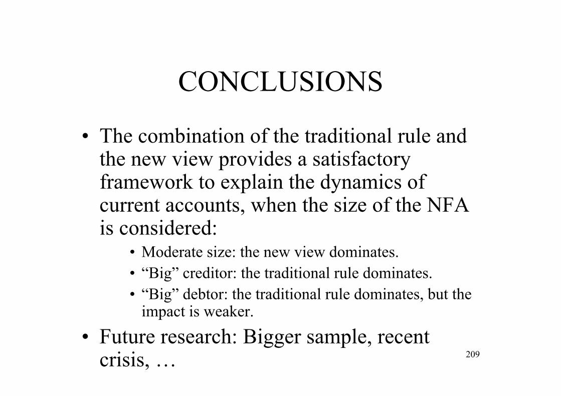
CONCLUSIONS
• The combination of the traditional rule and the new view provides a satisfactory framework to explain the dynamics of current accounts, when the size of the NFA is considered:
• Moderate size: the new view dominates.• “Big” creditor: the traditional rule dominates. • “Big” debtor: the traditional rule dominates, but the
impact is weaker.
• Future research: Bigger sample, recent crisis, … 209
6. CONCLUSIONS
210
CONCLUSIONS
• The literature on economic growth has provided many fruitful insights on many issues.
• However, many others remain unanswered, suggesting avenues for future research.
• When addressing an issue for research, I would recommend an appropriate mix of theoretical (adopting a model suitable for the objectives planned) and empirical contents.
211

REFERENCES
212
REFERENCES (Textbooks)
• Aghion, Philippe and Peter Howitt (1998), Endogenous growth theory, MIT Press.
• Aghion, Philippe and Peter Howitt (2009), Economics of growth, MIT Press.
• Barro, Robert and Xavier Sala i Martín (2004), Economic growth. Second edition,McGraw-Hill. Also in Spanish.
213
REFERENCES (Textbooks)
• Easterly, W. (2001), The Elusive Quest for Growth : Economists ’ Adventures and Misadventures in the Tropics, MIT Press. Also in Spanish.
• Weil, David N. (2009), Economic growth.Second edition, Pearson Addison Wesley.
214
REFERENCES (Others)
• Aghion, Philippe and Peter Howitt (1992), “A model of growth through creative destruction”, Econometrica, 60: 323-351.
• Arrow, Kenneth J. (1962), “The economic implications of learning by doing”, Review of Economics Studies, 29:155-173.
• Domar, Evsey (1946), “Capital expansion, rate of growth, and unemployment”, Econometrica, 14: 137-147.
215
REFERENCES (Others)
• Frankel, M. (1962), “The production function in allocation of growth: a synthesis”, American Economic Review, 52:995-1022.
• Harrod, Roy F. (1939), “An essay in dynamic theory”, Economic Journal, 49:14-33.
216
REFERENCES (Others)
• Lucas, Robert E., Jr (1988), “The mechanics of economic development”, Journal of Monetary Economics, 22:3-42.
• Romer, Paul M. (1990), “Endogenous technological change”, Journal of Political Economy, 98:71-102.
• Schumpeter, Joseph A. (1942). The theory of economic development. Harvard University Press.
• Solow, Robert M. (1956), “A contribution to the theory of economic growth”, Quarterly Journal of Economics, 70:65-94. 217
REFERENCES (Others)
• Solow, Robert M. (1957), “Technical change and the aggregate production function”, Review of Economics and Statistics, 39:312-320.
218

REFERENCES (Personal work)
• Kraay, Aart and Jaume Ventura (2000), “Current accounts in creditor and debtor countries”, Quarterly Journal of Economics 115:1137-1166.
• Lane, Philip R., and Gian Maria Milesi-Ferretti (2007), “The external wealth of nations mark II: revised and extended estimates of foreign assets and liabilities, 1970-2004”, Journal of International Economics 73: 223-250.
219

REFERENCES (Personal work)
• Erauskin, Iñaki (2008), “The sources of economic growth in Spain, the Basque Country, and Navarre during 1986-2004”, Investigaciones Regionales, 12:35-58.
• Erauskin, Iñaki (2011), “Accounting for growth in Spain, the Basque Country (and its three historic territories), Navarre, and Madrid since 1965”. Ekonomiaz, 78:272-309. 220
REFERENCES (Personal work)
• Erauskin, Iñaki (2009), “The current account and the new rule in a not-so-small open economy”, InvestigacionesEconómicas, vol. XXXIII(3):529-557.
• Erauskin, Iñaki (2015), “Savings, the size of the net foreign asset position, and the dynamics of current accounts”, International Review of Economics and Finance, 39: 353-370. 221


![Evaluación de tecnología Java para la implantación de …paginaspersonales.deusto.es/dipina/publications/ADIS-2003.pdf · más extendidos son Rational Unified Process (RUP) [13]](https://img.pdfslide.us/doc/110x75/5bb4993309d3f2317c8dbe24/evaluacion-de-tecnologia-java-para-la-implantacion-de-mas-extendidos-son.jpg)