Theories and Methods of First Order Ferroelectric Phase ...cdn.intechweb.org/pdfs/12502.pdf · barium titanate, lead zirconium titanate, ... kind of theory is often called Landau

16

Theories and Methods of First Order Ferroelectric Phase Transitions

C L Wang Shandong University

P R China

1. Introduction

Most ferroelectrics in practical applications are of first order phase transition, such as

barium titanate, lead zirconium titanate, etc. However, theoretical investigation of first order

phase transition is much more complicated than that of second order phase transitions.

Therefore in the chapter, theoretical treatments of ferroelectric phase transition of first order

are summarized. In the next section, results from thermodynamic theory are discussed. This

kind of theory is often called Landau theory, Landau-Devonshire theory or Landau–

Devoshire–Ginzburg theory in literatures. Basic concepts and definitions such as

characteristic temperatures, thermal hysteresis and field induced phase transition are

presented. In the third section, effective field approach for first order phase transition is

formulised. Even though this approach is a very simple statistic physics method, it supplies

a very helpful approach to understand many physical phenomena of first order phase

transitions. In the fourth section, results from Ising model in a transverse field under mean

field approximation are discussed. Then the equivalence of the model with effective field

approach is demonstrated. Also application of Monte Carlo simulation on Ising model with

four-spin couplings is included. In the last part, understanding of physical property of

relaxor ferroelectrics from point view of first order phase transition is addressed.

2. Thermodynamic theory of ferroelectrics

In this section, thermodynamic theory of first order ferroelectric phase transition is

formalized. Free energy is analyzed at first. Then definition of characteristic temperatures is

discussed. Afterwards temperature dependence of polarization and hysteresis loops are

shown for static situation. At last dynamic behavior of polarization under external electric

field is presented.

Formalism of thermodynamic description, or Landau theory for ferroelectrics can be found in many classical books (Blinc & Zeks ,1974; Lines & Glass, 1977), or from website like wikipedia (http://en.wikipedia.org/wiki/Ferroelectricity). Based on Landau theory, the free energy of a ferroelectric material, in the absence of an electric field and applied stress may be written as a Taylor expansion in terms of the order parameter, polarization (P). If a sixth order expansion is used (i.e. eighth order and higher terms truncated), the free energy is given by:

www.intechopen.com

Ferroelectrics

276

( )( ) ( ) ( )( ) ( ) ( ) ( )

2 2 2 4 4 4 2 2 2 2 2 40 0 11 12

6 6 6 4 2 2 4 2 2 4 2 2111 112

2 2 2123

1 1 1

2 4 21 1

6 61

6

Δ = α − + + + α + + + α + +⎡ ⎤+ α + + + α + + + + +⎣ ⎦

+ α

x y z x y z x y y z z x

x y z x y z y z x z x y

x y z

G T T P P P P P P P P P P P P

P P P P P P P P P P P P

P P P

(1)

where ΔG stands for the free energy difference of ferroelectric phase and that of paraelectric phase, Px, Py, and Pz are the components of the polarization vector in the x, y, and z directions respectively. The coefficients, αi,αij,αijk must be consistent with the crystal symmetry. To investigate domain formation and other phenomena in ferroelectrics, these equations are often used in the context of a phase field model. Typically, this involves adding a gradient term, an electrostatic term and an elastic term to the free energy. In all known ferroelectrics, α0 and α111 are of positive values. These coefficients may be obtained experimentally or from ab-initio simulations. For ferroelectrics with a first order phase transition, α11 is negative, and α11 is positive for a second order phase transition. The ferroelectric properties for a cubic to tetragonal phase transition may be obtained by considering the one dimension expression of the free energy which is:

( ) 2 4 60 0 11 111

1 1 1

2 4 6x x xG T T P P PΔ = α − + α + α (2)

The shape of above free energy is schematically shown in Fig. 1 at different temperatures for first order phase transitions. In the following numerical calculations, parameter values are

set as α0=1, T0=1, α11=-1and α111=1 in arbitrary unit for simplicity.

Fig. 1. Free energy for a first order ferroelectric phase transition at different temperatures

There are four characteristic temperatures in the phase transition process, i.e., Curie-Weiss temperature T0, Curie temperature Tc, ferroelectric limit temperature T1 and limit temperature

www.intechopen.com


277

of field induced phase transition T2. The Curie-Weiss temperature can be easily accessed

experimentally from the Curie-Weiss law of dielectric constant ε at paraelectric phase, i.e.,

0

p

C

T Tε = − (3)

In above expression, C is the Curie-Weiss constant, subscript p of ε stands for paraelectric phase. However the Curie temperature is less accessible experimentally. This temperature measures the balance of the ferroelectric phase and the paraelectric phase. At this temperature, the free energy of ferroelectric phase is the same as that of paraelectric phase. When temperature is between T0 and Tc, ferroelectric phase is stable and paraelectric phase is meta-stable, this can be easily seen in Fig.1. When the temperature is between Tc and T1, ferroelectric phase is in meta-stable state while paraelectric phase is stable. When the temperature is higher than T1, ferroelectric phase disappears. Normally, this temperature is corresponding to the peak temperature of dielectric constant when measured in heating cycle. In other words, peak temperature of dielectric constant measured in heating cycle is the ferroelectric limit temperature T1, not the Curie temperature Tc in a more precise sense. Between temperature T1 and T2, ferroelectric state still can be induced by applying an external electric field. The polarization versus the electric field strength is a double hysteresis loop, which is very similar with that observed in anti-ferroelectric materials. When the temperature is higher than T2, only paraelectric phase can exist. The characteristic temperatures Tc, T1 and T2 can be easily determined from Eq.(2) of free energy as following. The Curie temperature Tc can be obtained from the following two equations;

( ) 2 4 60 0 11 111

1 1 10

2 4 6c x x xG T T P P PΔ = α − + α + α = (4)

( ) 3 50 0 11 111 0c x x x

x

GT T P P P

P

∂Δ = α − +α +α =∂ (5)

The first equation means that the free energy of ferroelectric phase is same as that of paraelectric phase, and the second equation implies that the free energy of ferroelectric phase is in minimum. From above two equations, we can have the expression of the Curie temperature Tc as

211

0

0 111

3

16cT T

α= + α α (6)

At the ferroelectric limit temperature T1, free energy has an inflexion point at Ps, the spontaneous polarization. As can be seen from Fig. 1, when temperature is below T1, free

energy has are three minima, i.e., at P=±Ps, and P=0. Above temperature T1, there is only one minimum at P=0. The spontaneous polarization can be obtained from the minimum of the free energy as,

( )( )

3 50 0 11 111

2 40 0 11 111

0

0

x x x

x

x x x

GT T P P P

P

P T T P P

∂Δ = α − +α +α =∂⎡ ⎤α − +α +α =⎣ ⎦

(7)

www.intechopen.com

Ferroelectrics

278

Since Px = 0 corresponds to a free energy maxima in the ferroelectric phase, the spontaneous polarization Ps is obtained from the solution of the equation:

( ) 2 40 0 11 111 0x xT T P Pα − +α +α = (8)

which is

( )2 211 11 0 111 0

111

14

2xP T T⎡ ⎤= −α ± α − α α −⎣ ⎦α (9)

Hence at temperature T1, we have

( )211 0 111 1 04 0T Tα − α α − = (10)

In a more explicitly form,

211

1 0

0 111

1

4T T

α= + α α (11)

Between temperature T1 and T2, there are still inflexion points, which means ferroelectric phase can be induced by an external electric field. When temperature is above T2, the inflexion points disappear. By taking the second derivative of the free energy Eq.(2), we can have the solution of the inflexion points,

( )22 4

0 2 0 11 11123 5 0x x

x

GT T P P

P

∂ Δ = α − + α + α =∂ (12)

( ) ( )2211 11 0 111 0

111

13 3 20

10xP T T⎡ ⎤= − α ± α − α α −⎢ ⎥⎣ ⎦α (13)

That is the polarization at the inflexion points. The limit temperature of the induced phase

transition T2 can be determined by

( ) ( )2

11 0 111 2 03 20 0T Tα − α α − = (14)

or

211

2 0

0 111

9

20T T

α= + α α (15)

The temperature dependence of the spontaneous can be calculated from Eq.(9) by

elimination of solutions yielding a negative square root (for either the first or second order

phase transitions) gives:

( )211 11 0 111 0

111

14

2xP T T⎡ ⎤= −α ± α − α α −⎣ ⎦α (16)

The temperature dependence of the spontaneous polarization from above equation is shown in Fig. 2. The four characteristic temperatures are denoted by light arrows. The dark arrows

www.intechopen.com


279

indicate the temperature cycles. Theoretical temperature hysteresis is ΔT=T1-T0. Experimentally, the temperature hysteresis could be larger than this value because of the polarization relaxation process. The hysteresis loop (Px versus Ex) may be obtained from the free energy expansion by adding an additional electrostatic term, Ex Px, as follows:

( ) 2 4 60 0 11 111

1 1 1

2 4 6x x x x xG T T P P P E PΔ = α − + α + α − (17)

( ) 3 50 0 11 111 0x x x x

x

GT T P P P E

P

∂Δ = α − +α +α − =∂ (18)

( ) 3 50 0 11 111x x x xE T T P P P= α − +α +α (19)

Fig. 2. Temperature dependence of the spontaneous polarization

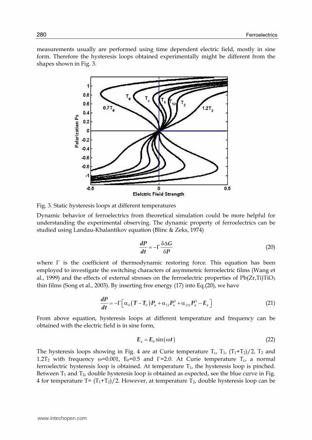
Plotting Ex as a function of Px and reflecting the graph about the 45 degree line gives an 'S' shaped curve when temperature is much lower than the transition temperatures, as can be seen from curves in Fig. 3. The central part of the 'S' corresponds to a free energy local

maximum, since the second derivative of the free energy ΔG respect polarization Px is negative. Elimination of this region and connection of the top and bottom portions of the 'S' curve by vertical lines at the discontinuities gives the hysteresis loop. Temperatures are labeled by each curve, label of 0.7T0 in Fig. 3 is for temperature T=0.7T0, and 1.2T2 is for T=1.2T2, T12 stands for T=(T1+T2)/2. When the temperature is below Curie temperature Tc, normal ferroelectric hysteresis loops can be obtained. When the temperature is between T1 and T2, double hysteresis loop or pinched loop could be observed. That means ferroelectric state is induced by the applied electric field. When the temperature is higher than T2, the polarization versus electric field becomes a non-linear relation, see 1.2T2 curve in Fig. 3. It should point out that curves in Fig. 3 are obtained under static electric field. Experimental

www.intechopen.com

Ferroelectrics

280

measurements usually are performed using time dependent electric field, mostly in sine form. Therefore the hysteresis loops obtained experimentally might be different from the shapes shown in Fig. 3.

Fig. 3. Static hysteresis loops at different temperatures

Dynamic behavior of ferroelectrics from theoretical simulation could be more helpful for understanding the experimental observing. The dynamic property of ferroelectrics can be studied using Landau-Khalantikov equation (Blinc & Zeks, 1974)

dP G

dt P

δΔ= −Γ δ (20)

where Γ is the coefficient of thermodynamic restoring force. This equation has been

employed to investigate the switching characters of asymmetric ferroelectric films (Wang et

al., 1999) and the effects of external stresses on the ferroelectric properties of Pb(Zr,Ti)TiO3

thin films (Song et al., 2003). By inserting free energy (17) into Eq.(20), we have

( ) 3 50 0 11 111x x x x

dPT T P P P E

dt⎡ ⎤= −Γ α − +α +α −⎣ ⎦ (21)

From above equation, hysteresis loops at different temperature and frequency can be obtained with the electric field is in sine form,

( )0 sinxE E t= ω (22)

The hysteresis loops showing in Fig. 4 are at Curie temperature Tc, T1, (T1+T2)/2, T2 and

1.2T2 with frequency ω=0.001, E0=0.5 and Γ=2.0. At Curie temperature Tc, a normal ferroelectric hysteresis loop is obtained. At temperature T1, the hysteresis loop is pinched. Between T1 and T2, double hysteresis loop is obtained as expected, see the blue curve in Fig. 4 for temperature T= (T1+T2)/2. However, at temperature T2, double hysteresis loop can be

www.intechopen.com


281

still observed because of the finite value of relaxation time. Higher than T2, no hysteresis can be observed, but a non-linear P-E relation curve. Similar shapes of hysteresis loops have been observed in PbxSr1-xTiO3 ceramics recently(Chen et al., 2009).

Fig. 4. Dynamic hysteresis loops at different temperatures with frequency ω=0.001. Dark loop is at Curie temperature Tc, red curve is for T1, blue curve for (T1+T2)/2, green curve for T2, and dark line for T=1.2T2.

To get insight understanding of the influence of the frequency on the shape of the hysteresis,

more hysteresis loops are presented in Fig. 5. The frequency is set as ω=0.001 for green

curves, ω=0.01 for red curves and ω=0.03 for blue curves at Curie temperature Tc, T1, (T1+T2)/2 and at T2 respectively. At Curie temperature Tc, see Fig. 5(a), the coercive field increases with increasing of measure frequency, but the spontaneous polarization is less influenced by the frequency. At temperature T1, this temperature corresponding to the peak temperature of dielectric constant when measured in heating cycle, pinched hysteresis loop can be observed at low frequency, see the green curve in Fig. 5(b). At higher frequency, the loop behaves like a normal ferroelectric loop, see blue curve in Fig.5(b). When temperature is between T1 and T2, as shown in Fig. 5(c) for temperature at T=(T1+T2)/2, typical double hysteresis loop can be observed at low frequency. When the frequency is higher, it becomes a pinched loop. This trend of loop shape can be kept even when temperature is up to T2, see curves in Fig. 5(d). Temperature dependence of polarization at different temperature cycles can be also obtained from Eq.(21) with a constant electric field E=0.01. The results are shown in shown

in Fig. 6 with different Γ, the coefficient of thermodynamic restore force. The dark line is for the static polarization, red curves are field heating, blue curves are field cooling. Solid lines

are for Γ=100, and dash-dotted lines are for Γ=10. The temperature hysteresis from the static theory, as indicated by the two dark dash lines, is smaller than that from Landau-

Khalanitkov theory. In other words, temperature hysteresis ΔT measured experimentally would be usual larger than that from static Landau theory. Also the temperature hysteresis

ΔT depends on Γ, since Γ is related with the relaxation time. A larger Γ represents small

www.intechopen.com

Ferroelectrics

282

relaxation time, or quick response of polarization with electric field. Hence ferroelectrics

with long relaxation time, i.e., small Γ, would expect a very larger temperature hysteresis.

Fig. 5. Hysteresis loops with frequency ω=0.001 for green curves, ω=0.01 for red curves and

ω=0.03 for blue curves at temperature (a) Tc; (b) T1; (c) (T1+T2)/2, (d) T2

Fig. 6. Temperature dependence of polarization at different temperature cycles. Dark line is for the static polarization. Red curves are field heating, blue curves are field cooling. Solid lines

are for short relaxation time(larger Γ), and dash-dot lines are for lone relaxation time (small Γ).

www.intechopen.com


283

3. Effective field approach

The effective field approach has proved to be a simple statistic physics method but valuable way to describe phase transitions (Gonzalo, 2006). The main supposition of this model is that each individual dipole is influenced, not only by the applied electric field, but by every dipole of the system. In its simplest form, which takes into account only dipole interactions, describes fairly well the main features of continuous ferroelectric phase transitions, i.e. second order phase transition. The inclusion of quadrupolar and higher order terms into the effective field expression is necessary for describing the properties of discontinuous or first order phase transitions (Gonzalo et al., 1993; Noheda et al., 1993, 1994). The effective field approach has turned out to be successful explaining the composition dependence of the Curie temperature in mixed ferroelectrics systems (Ali et al., 2004; Arago et al., 2006). A quantum effective field approach has also been developed for phase transitions at very low temperature (Gonzalo, 1989; Yuan et al., 2003; Arago et al., 2004) in ferro-quantum paraelectric mixed systems. In this section, quantum effective field approach is adopted to reveal the influence of the zero point energy on first order phase transitions (Wang et al., 2008). We can see that when the zero point energy of the system is large enough and the ferroelectric phase is suppressed, a phase transition-like temperature dependence of the polarization can be observed by applying an electric field. The effective field, as described in detail in Gonzalo’s book (Gonzalo, 2006), can be expressed as

3 5effE E P P P= +β + γ + δ +A (23)

where E is the external electric field, and the following terms correspond to the dipolar, quadrupolar, octupolar, etc., interaction. By keeping the first two terms, i.e. dipolar and quadrupolar interaction, gives account of the first order transition. From statistical considerations, the equation of state is,

3( )

tanh tanheff

B B

E E P PP N N

k T k T

μ⎛ ⎞ ⎛ ⎞+β + γ μ= μ = μ⎜ ⎟ ⎜ ⎟⎝ ⎠ ⎝ ⎠ (24)

where N is the number of elementary dipoles per unit volume, μ is the electric dipole moment, kB is the Boltzmann constant, and T is the absolute temperature. The Curie temperature is given by

2

C

B

NT

k

β μ=

The explicit form of the equation of state can be rewritten from Eq.(24),

1 3tanhBk T PE P P

N− ⎛ ⎞= −β − γ⎜ ⎟μ μ⎝ ⎠ (25)

In order to handle easier this expression, following normalization quantities are introduced,

2 2

2; ; ; B

C

k TE P T Ne p t g

N N T N

γ μ≡ ≡ ≡ = ≡β μ μ β μ β

www.intechopen.com

Ferroelectrics

284

so Eq. (25) is rewritten as

3

tanhe p g p

pt

⎛ ⎞+ + ⋅= ⎜ ⎟⎝ ⎠ (26)

or

1 3tanhe t p p gp−= ⋅ − − (27)

and as in absence of external field e = 0, p = pS

3

1tanhS S

S

p gpt

p−+= (28)

Fig.7 shows the plot of the normalized spontaneous polarization pS versus normalized temperature t obtained from Eq. (28) for several values of the parameter g. As it is shown in the discussion of the role of the quadrupolar interaction in the order of the phase transition (see Gonzalo et al., 1993; Noheda et al., 1993; Gonzalo, 2006), values of g smaller than 1/3 correspond to a second order, or continuous phase transition, and values larger than 1/3 indicate that the transition is discontinuous, that is, first order. In this case, a spontaneous

polarization pθ exists at temperature Tθ>TC, and then τθ>1, being Δt = tθ -1 the corresponding reduced thermal hysteresis, which is the signature of the first order transitions.

Fig. 7. Temperature dependence of the spontaneous polarization for different quadrupolar

interaction coefficient g. The inset shows the polarization discontinuity pθ(g) and the thermal

hysteresis temperature Δt(g) in a first order transition.(Wang et al., 2008)

In order to determine pθ(g), deriving in Eq. (28),

0S p

t

pΘ

∂ =∂

www.intechopen.com


285

and pθ(g) can be obtained from

( )( ) ( )2 2 1 31 1 3 tanh 0p gp p p gp−θ θ θ θ θ− + − + = (29)

Substituting pθ(g) in Eq. (28) again we obtain tθ(g). The inset of Fig.7 shows pθ(g) and Δt(g)

respectively. It can be seen that Δt grows almost linearly with g and that pθ approaches to a

saturation value that, resolving Eq.(29), turns out to be pθ = 0.8894 when g→ ∞. When a phase transition takes place at very low temperature it is necessary to consider quantum effect. The energy of the system is no longer the classical thermal energy kBT, but the corresponding energy of the quantum oscillator,

0

1

2E n

⎛ ⎞= ω +⎜ ⎟⎝ ⎠¥

being E0= ħω0/2 the zero point energy, and <n> the average number of states for a given temperature T. From this quantum energy expression we can obtain a new temperature scale TQ (see Arago et al., 2004) defined as,

( )0

00 /

0

1 1

2 1 2 tanh /2B

Q QBk T

B B

k T Te k k Tω

ω⎛ ⎞ω + ≡ ⇒ ≡⎜ ⎟− ω⎝ ⎠¥

¥¥¥

(30)

and then, the corresponding quantum normalized temperature, tQ ≡ TQ/TC. If we introduce a new normalization for the zero point energy

0 02

/2

B C

E

k T N

ωΩ ≡ = β μ¥

so we can rewrite,

( )tanh /Qt

t

Ω≡ Ω (31)

and Eq. (27) and (28) become respectively,

1 3tanhQe t p p gp−= − − (32)

( )3

1, e 0

tanh / tanhQ S S

S

p gpt

t p−+Ω≡ = =Ω (33)

The temperature dependence of the spontaneous polarization can be found from above equation for a given value of g and different values of the parameter Ω. Fig. 8 plots pS(t) with g = 0.8 to ensure it is a first order transition. The influence of the zero-point energy is quite obvious: when it is small, the phase transition is still of normal first order one. As the zero point energy increases, both the transition temperatures and the spontaneous polarization

decrease. The Curie temperature goes to zero for Ω = 1, but no yet tθ, neither the saturation spontaneous polarization does. From the definition of the normalized zero point energy Ω, we can see then that the Curie temperature goes to zero when the zero point energy is the same as the classical thermal energy kBTC. Imposing again the condition of the zero slope,

www.intechopen.com

Ferroelectrics

286

(∂t/∂pS)pθ= 0, we can obtain pθ(Ω), and then tθ(Ω), which must be zero when the ferroelectric behavior will be completely depressed. In this way we work out the zero point energy critical value (Ωcf = 1.1236 for g=0.8) that would not allow any ordered state. Furthermore,

from the condition tθ(Ωcf, g) = 0, we will find the relationship between the critical zero point energy Ωcf and the strength of the quadrupolar interaction given by the coefficient g. Fig. 9 plots Ωcf (g) that indicates that Ωcf grows almost linearly with g, specially for larger values of g. This means that ferroelectrics with strong first order phase transition feature needs a relative large critical value of zero point energy to depress the ferroelectricity.

Fig. 8. Temperature dependence of the spontaneous polarization at different zero point energy. All curves correspond to a quadrupolar interaction coefficient g=0.8. (Wang et al., 2008)

Above results prove that a ferroelectric material, with strong quadrupolar interaction, undergoes a first order transition (g>1/3) unless its zero point energy reaches a critical

value, Ωcf, because in such case the phase transition is inhibited. However, an induced phase transition must be reached by applying an external electric field. Let be a system with g= 0.8,

and Ω=1.6, that is a first order ferroelectric with a zero point energy above the critical value and, hence, no phase transition observed. And let us apply a normalized electric field e that will produce a polarization after Eq. (32). Fig. 10 plots p(t) for different values of the electric field. It can be seen that when it is weak (see curves corresponding to 0.01 and 0.02), the polarization attains quickly a saturation value, similar to what is found in quantum paraelectrics. The curve of e=0.03 (see the dashed line) is split into two parts. The lower part would represent a quantum paraelectric state, but the upper part stands for a kind of ferroelectric state. Therefore there exists a critical value between e=0.02 and 0.03, which is the minimum electric field for inducting a phase transition. For 0.04<e<0.06 the induced polarization curve shows a discontinuous step, but as the electric field increases, 0.07, 0.08 and so on, the polarization changes continuously from a large value at low temperature to a relative small value at high temperature, showing a continuous step. So there is another critical electric field somewhere in between 0.05<e<0.07, separates the discontinuous step

www.intechopen.com


287

and the continuous step of the induced polarization. In fact, this tri-critical point would be around e=0.06. It is also important to remark that the above-mentioned features of the field induced phase transitions have been observed in lead magnesium niobate (Kutnjak et al., 2006), which is a well-known ferroelectric relaxor.

Fig. 9. Quadrupolar interaction dependence of the critical zero point energy Ωcf that depress ferroelectricity. (Wang et al., 2008)

Fig. 10. Temperature dependence of the field induced polarization for Ω=1.15 and g=0.8. The parameter is the strength of the electric field. (Wang et al., 2008)

www.intechopen.com

Ferroelectrics

288

For further understanding the field induced phase transitions, Fig. 11 shows the hysteresis loops obtained numerically from Eq. (32) and corresponding to the curves displayed in Fig. 10. Double hysteresis loops can be observed when the temperature is lower than a critical point, around t=0.6, suggesting that ferroelectricity can always be induced at very low temperature. When the temperature is higher than this critical value, there is no hysteresis loop and we can just observe a non-linear p–e behaviour (see for instance the case for t=0.7).

However, when the electric field is lower than e≈0.025, as indicated by the dashed arrow in Fig. 11, no hysteresis loop can be observed. That is the case corresponding to the curves e =0.01 and 0.02 in Fig. 10. The critical electric field able to induce a phase transition logically increases with the increasing of temperature, so at lower temperature region in Fig. 10, we can always have field induced ferroelectricity when the applied electric field is strong enough.

Fig. 11. Hysteresis loops at different temperatures for Ω=1.15 and g=0.8. The dashed arrow indicates the minimum electric field needed to induce a ferroelectric state at t=0. (Wang et al., 2008)

To understand the influence of the zero point energy on the shape of hysteresis loop, here we take the case of g=0.8 at t=0 as example. The corresponding quantum temperature, after Eq. (31), is

( )0Qt t = = Ω

and then, Eq. (32) becomes

1 3tanhe p p gp−= Ω − − (34)

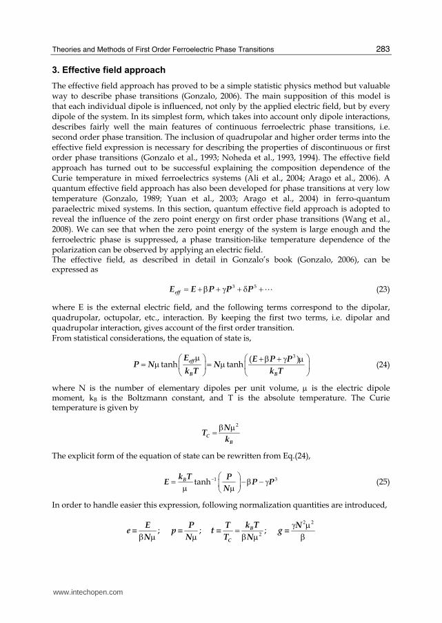
Fig. 12 plots the hysteresis loops calculated after Eq. (34). When the zero point energy is smaller than the critical value Ωcf (Ωcf=1.1236, in this case) a normal hysteresis loop is obtained, where the coercive field decreases as zero point energy increases. For the critical value, a double hysteresis loop with zero coercive field is found. But if we continue

www.intechopen.com


289

increasing the zero point energy, we arrive to a point where no hysteresis loop is found at all. That suggests that above this other critical value, be Ωcp, there is no way to induce a phase transition, even applying a strong field, and the system remains always in a paraelectric state.

Fig. 12. Hysteresis loops at zero temperature for different zero point energy values. The critical value of Ωcf is the minimum zero point energy for the system to have ferroelectricity, while the critical value of Ωcp is the maximum zero point energy for the system to get field induced ferroelectricity. (Wang et al., 2008)

From the analysis of the hysteresis loops in Fig.12 we can determine the critical electric field needed to induce phase transition imposing the conditions,

2

20, 0

cp

e e

p p

⎛ ⎞ ⎛ ⎞∂ ∂= >⎜ ⎟ ⎜ ⎟∂ ∂⎝ ⎠ ⎝ ⎠

and deriving in Eq. (34) we get,

( )2

22 2

21 3 0, 6 0

1 1c c

c c

gp g pp p

⎛ ⎞Ω Ω⎜ ⎟− − = − >⎜ ⎟− −⎝ ⎠ (35)

hence we obtain,

( ) ( ) ( )2

23 1 3 1 6 2

6c

g g gp

g

− + − Ω−= (36)

Substituting pc (g, Ω) obtained after Eq. (36) into Eq. (34) we can get the coercive field ec (pc) at zero temperature. Besides, as it is showed in Fig. 12, when the zero point energy attains its critical value Ωcf, the coercive field turns out to be zero, so this is another way to check

www.intechopen.com

Ferroelectrics

290

the quadrupolar interaction dependence of the critical zero point energy Ωcf(g) as displayed in Fig.9. It must be noted the full accordance between the two calculations. At the second critical value of the zero point energy, Ωcp, the hysteresis loop becomes an inflexion e-p curve as it can also be observed in Fig.12, so in this case both Eq. (35) must be equal to zero, and by solving the system of equations, it results,

( )23 1 3 1

,12 6

cp cp

g gp

g g

+ −Ω = = (37)

The phase diagram at zero temperature is shown in Fig. 13. It displays the role of both the quadrupolar interaction strength and the zero point energy on first order phase transitions. On the top of this diagram we find just paraelectric state (PE), while on the bottom left it appears only second order phase transitions (FE: 2nd order) that correspond to g < 1/3 and Ω ≤ 1. On the bottom right (g > 1/3) there are the first order transitions (FE: 1st order) as the critical values of the zero point energy (Ωcf >1) that depress the ferroelectricity grow monotonously with g. Above the curve Ωcf(g) there are induced electric field phase transitions (first order also). They are limited by another curve Ωcp(g) given by Eq. (37) indicating that no phase transition can be observed when the zero point energy of the system is greater than this value.

Fig. 13. Phase diagram of zero point energy critical value Ωc versus quadrupolar interaction coefficient g at zero temperature. The second order phase transition region is denoted as “FE:2nd order”, “FE:1st order” indicates a normal first order transition, “iFE” is the region of induced ferroelectric phase and on the top, “PE” corresponds to the paraelectric phase. (Wang et al., 2008)

From above calculations in the framework of effective field approach, it can be seen that a phase transition can be induced by applying an electric field in a first order quantum paraelectric material. There exist two critical values of the zero point energy, one is Ωcf that depress ferroelectricity, and another is Ωcp above which it is impossible to induce any kind

www.intechopen.com


291

of phase transition independently of the value of the electric field applied. Phase diagram is presented to display the role of both the quadrupolar interaction strength and the zero point energy on the phase transitions features.

4. Ising model with a four-spin interaction

Ising model in a transverse field with a four-spin interaction has been used to study the first-order phase transition properties in many ferroelectric systems. Under the mean-field approximation, first-order phase transition in ferroelectric thin films (Wang et al., 1996; Jiang et al., 2005) or ferroelectric superlattices (Qu, Zhong & Zhang, 1997; Wang, Wang & Zhong, 2002) have been systematically studied. Using the Green’s function technique, the first-order phase transition properties in order-disorder ferroelectrics (Wang et al., 1989) and ferroelectric thin films (Wesselinowa, 2002) have been investigated. Adopting the higher-order approximation to the Fermi-type Green’s function, the first-order phase transition properties have been studied in the parameter space with respect to the ratios of the transverse field and the four-spin interaction to the two-spin interaction for ferroelectric thin films with the uniform surface and bulk parameters (Teng & Sy,2005). These works prove that Ising model with four-spin interaction is a successful model for studying first order phase transition of ferroelectrics. In the following, basic formulism under mean-field approximations and Monte Carlo simulation are presented, and the results are discussed.

4.1 Mean field approximation

The Hamiltonian of the transverse field Ising model with a four-spin interchange interaction

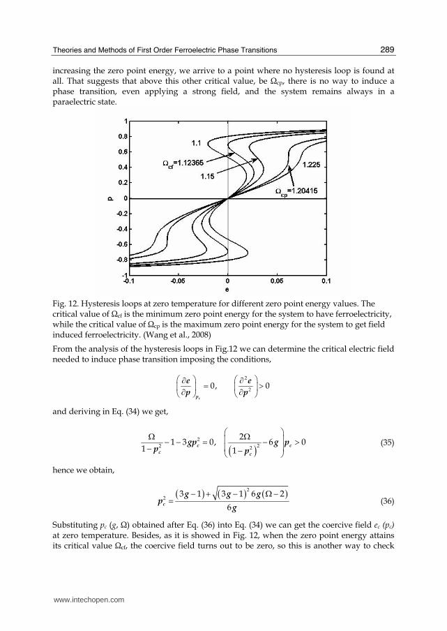
term is (Wang et al., 1989; Teng & Sy, 2005):

( ) ( )2 4

, , , ,

x z z z z z zi i ij i j ijkl i j k l

i i j i j k l

H S J S S J S S S S= − Ω − −∑ ∑ ∑ (38)

where Ω is the transverse field, Sx and Sz are the x and z components of pseudospin-1/2

operator, J(2) and J(4) are the two-spin and four-spin exchang interaction, subscript i,j,k,l are

site number, summation run over only the nearest-neighbor sites. Under the mean field

approximation (Blinc & Zeks ,1974), solutions of Hamiltonian Eq.(38) is,

34

tanh2 2

0

2tanh

2 2

x ii

i B

yi

z zi iz i

i

i B

FS

F k T

S

J S J S E FS

F k T

⎧ ⎛ ⎞Ω⎪ = ⎜ ⎟⎪ ⎝ ⎠⎪⎪ =⎨⎪⎪ + + μ ⎛ ⎞=⎪ ⎜ ⎟⎪ ⎝ ⎠⎩

where

2

2 4 2z z z zi ij j ijkl j k l

ij ijkl

F J S J S S S E< > < >⎛ ⎞= Ω + + − μ⎜ ⎟⎜ ⎟⎝ ⎠∑ ∑

For a homogenous system

www.intechopen.com

Ferroelectrics

292

z z z z zi j k lS S S S S= = = =

4, ' ,ij ijkl ij jkl

J J J J F F= = =∑ ∑

Therefore we have,

' 3 2

tanh2 2

zi

B

JR J R E FR S

F k T

⎛ ⎞+ + μ= = ⎜ ⎟⎝ ⎠ (39)

( )22 3' 2F JR J R E= Ω + + + μ (40)

The polarization is related to the z-component spin average as,

2 2ziP N S N R= μ = μ (41)

Following normalizations are introduced to handle easier this expression,

4' 4' , , , , , 2Bk TJ F E Pg t e p R

J J J J J N

Ω μ= ω = = τ = = = =μ

Eq.(39) and (40) can be rewritten as,

' 3 /4 2

tanh2

p g p ep

t

+ + τ⎛ ⎞= ⎜ ⎟τ ⎝ ⎠ (42)

232 '

2 8 2

p p eg

⎛ ⎞τ = ω + + +⎜ ⎟⎝ ⎠ (43)

In the absence of transverse field, i.e., ω=0 in Eq.(43), and by defining quadrupolar contribution factor g as,

4'

4 4

g Jg

J= = ⋅

Eq.(42) can be rewritten in the same form in Eq. (26), which is obtained from effective field approach. The equivalence of effective field approach and Ising model with four spin couplings under mean field approximation is completely approved. Therefore the critical value of relative quadrupolar contribution is gc=1/3 under mean field approximation for occurrence of first order phase transition.

4.2 Monte Carlo simulation

A well known and useful method to study phase transitions is by means of the Monte Carlo simulations (Binder, 1984). In particular, phase transitions in Ising systems of relatively low dimensions are sufficient to carry out numerical simulations in the vicinity of the transition temperature, providing a good empirical basis to investigate the asymptotic behavior at the phase transition (Gonzalo & Wang, 2008). Here Monte Carlo simulation is applied to the

www.intechopen.com


293

Ising model with four-spin coupling for studying the phase transition behavior, especially checking the critical value from the four-spin coupling strength, or quadrupolar contribution (Wang et al., 2010). Monte Carlo method with metropolis algorithm has been used to simulate 3D Ising cubic lattice. The Hamiltonian is same as in Eq.(38), but without the first term, i.e., without including the tunneling term. In this case, the critical value of the four-spin coupling contribution under mean field approximation is

( )12 ' 2 ' 1, '/ 1/6

3c c

J Jg J J

J J= = = =

The critical four-spin coupling strength is J’/J=1/6 from mean field theory, which is a reference value for the Monte Carlo simulations. Periodic boundary condition has been used

in the simulations. The lattice size is denoted as N=L×L×L, where L is edge length. In the Monte Carlo simulation, edge length L=20, 30, 100 are used. Monte Carlo steps are chosen different for different lattices size to achieve an adequate accurate of the results.

Fig. 14. Temperature dependence of spin average (a) and reduced average energy of cubic lattice with edge length L=20 and 30 for different four-spin coupling strength J’/J. (Wang et al., 2010)

Simulation is started with relative small lattice size, with edge length L=20 and 30. The temperature dependence of the spin average and the reduced average energy with different four-spin coupling strength are presented in Fig.14. The reduced average energy is defined as the energy with respective to the ground state energy E0 in the temperature of zero Kelvin. The curve for lattice size L=20 is marked by solid symbols, and that for L=30 is marked by open symbols. The temperature is in the scale of two-site coupling J. As the four-spin coupling strength increases from J’/J =0 to J’/J =1, the transition temperature is shifted to higher temperature. The decreasing of the average spin and the increasing of the reduced average energy, with increasing temperature around the transition temperature becomes more rapidly as J’/J increases. The general difference between L=20 and that of L=30 is marginal except around the transition temperatures. Even though the four-spin coupling

www.intechopen.com

Ferroelectrics

294

strength (J’/J) is much larger than that of the mean field value 1/6, the first order transition characteristic is not such obvious in these two lattice sizes. The temperature dependence of spin average and the reduced average energy of lattice size 100 is shown in Fig.15 for different four-spin coupling strength J’/J. The value of J’/J increases from 0.0 to 1.1 with increment of 0.1, corresponding the curves from left to right. The general behavior seems similar with that for L=20 and 30 as shown in Fig.14. However, with increasing of the four-spin coupling strength J’/J, as can be seen in the most right side curve of J’/J=1.1 in Fig.15(a), the spin average drops down around the transition temperature very quickly, showing a discontinuous feature. Similar discontinuous feature can be also seen in the reduced average energy curves in Fig.15(b). The reduced average energy goes up very sharply around the transition temperature for J’/J=1.1, as shown in the most right side curve in Fig.15(b). From Fig.15(b), we also notice that there is an inflexion point around the transition temperatures. The reduced average energy at this point is about 1/3 of the ground state energy when J’/J is larger. This condition could supply a criterion for determine the transition temperature in the first order phase transition.

Fig. 15. Temperature dependence of spin average (a) and reduced average energy (b) of lattice size L =100 for with different four-spin coupling strength J’/J. (Wang et al., 2010)

To determine the transition temperature, we appeal the calculation of the Binder cumulant.

The temperature dependence of the Binder cumulant for J’/J= 1.0 with different lattice size

are shown in Fig.16. For lattice size of L=10, 20, 25, 30 and 40, the Binder cumulant does

cross the point at Tc=8.148J. For lattice size L is larger, see L= 50, 70, 100 and 150, the Binder

cumulant misses the cross point, and drops down from 2/3 to a very small value at higher

temperatures. That means that the transition temperature can not be obtained from the

Binder cumulant when the four-spin coupling strength J’/J is larger. It is believed that the

Binder cumulants in Fig.16 suggesting the transition is of second order when the lattice size

is smaller than L=40, and the transition is of first order when the lattice size is larger than

L=40. The lattice size L=40 is around the critical lattice size for four-spin coupling strength

J’/J =1. This also implies that the transition temperature of first order transition is lattice size

dependent.

www.intechopen.com


295

Fig. 16. Binder cumulants for J’/J= 1.0 with different lattice sizes. The circle indicates the cross point of the Binder cumulants for lattice size L<40. (Wang et al/, 2010)

0.980 0.985 0. 990 0.995 1.000 1. 005 1.010

0.0

0.1

0.2

0.3

0.4

0.5

0.6

0.7

0.8

0.9

J '=0. 00 J '=0. 10 J '=0. 20

J '=0. 30 J '=0. 40

J'=0.50 J '=0. 60

J'=0.70 J '=0. 75

J '=0. 80 J '=0. 90

J '=1. 00 J '=1. 10

Sp

in A

ve

rag

e 2

<S

>

Te mperature T /Tc

0. 980 0.985 0.990 0. 995 1.000 1.005 1. 010-0.8

-0.7

-0.6

-0.5

-0.4

-0.3

<E

>/E

0

Tempe rature T /Tc

J'=0 .00 J'=0 .10

J'=0 .20 J'=0 .30

J'=0 .40 J '=0 .50

J'=0 .60 J '=0 .70

J'=0 .75 J'=0 .80

J'=0 .90 J'=1 .00

J'=1 .10

Fig. 17. Temperature dependence of spin average of lattice sizes L=100 for different J’/J around the transition temperature. Temperature is scaled by the transition temperature determined by the criterion <E>/E0=1/3. (Wang et al., 2010)

Fig.17 shows the temperature dependence of spin average and the reduced average energy of lattice size 100 as shown in Fig.15, but with temperature rescaled by the transition temperature TC. The transition temperature TC is determined by the criterion of the averaged energy being one third of the ground state energy, i.e., temperature at <E>/E0=1/3 being the transition temperature, as circled in Fig.17(b). Results from Monte Carlo simulations on Ising cubic lattices with four spin couplings suggest that, (1) critical value of four-spin coupling strength for occurrence of first order

www.intechopen.com

Ferroelectrics

296

phase transition is larger than that of mean field theory; (2) the critical value is lattice dependence. When lattice size is smaller, the phase transition is still of second order; (3) when the phase transition is of first order, the transition temperature can be determined by the average energy being a third of the ground state energy. However, this criterion has not been justified rigorously.

5. Ferroelectric relaxors

Ferroelectric relaxors have been drawn much attention because of their high electromechanical performance and unusual ferroelectric properties. Two review articles (Ye, 1998; Bokov & Ye, 2006) have summarized the achievements of recent researches on ferroelectric relaxors, especially for lead magnesium nibate (PMN). Basically, there are two categories of explanations about the fundamental physics of their unusual properties. One is based upon the randomness of their compositions and structures, such as Smolenskii’s theory and spherical random bond random field model. Another is presumably based upon the experimental phenomenon, such as macro-micro-domain and super-paraelectric model. In this section, a general explanation of the properties observed in ferroelectric relaxors is proposed after analysis of the later category models (Wang et al., 2009). Field induced phase transition and diffused phase transition are reproduced within the framework of effective field approach. Interpretation is started with the experimental results of field induced phase transition in PMN. The temperature dependence of the polarization under different electric field strengths has been obtained (Ye & Schmid, 1993; Ye, 1998). From this relation we can understand that (1) there is no ferroelectric phase transition in the whole temperature range, since there is no spontaneous polarization as the temperature goes down to zero Kelvin; (2) ferroelectricity can be induced by an external electric field. These imply that the phase transition in PMN is of first order, but the ferroelectricity is depressed in the whole temperature range. To understand these characteristics of ferroelectric relaxors, we can recall the temperature dependence of the spontaneous polarization in a typical normal first order ferroelectric phase transition is shown in Fig. 2. This implies that PMN is in a paraelectric state, but not far from the ferroelectric state. Apart from the field induced phase transition, the following features should be also found within this temperature range in a normal first order ferroelectric phase transition: (1) a very long relaxation time, because of the critical slow down as the temperature is near the critical temperature. (2) super-paraelectric behavior. Normally there should be a double hysteresis loop observed in this temperature range. However, the double hysteresis loop could be reduced to a super-paraelectric shape because of the long relaxation time of the critical slow down. (3) macro-micro-domain crossover. As the temperature is much lower than the critical temperature, single domain or macro-domain is expected since it is in ferroelectric state; as the temperature is much higher than the critical temperature, no domain will be observed as it is in paraelectric state. Around the critical temperature, macro-micro-domain crossover is expected, i.e., polar nano-regions are forming in this temperature range. All these features have been observed in the ferroelectric relaxors like PMN. The depression of the ferroelectricity in PMN reminds us of the case of quantum paraelectrics SrTiO3. Therefore the field induced phase transition in a first order phase transition depressed by quantum fluctuation has been investigated within the framework of effective field approach by inclusive of zero point energy (Wang et al., 2008). The

www.intechopen.com


297

temperature dependence of the induced polarization under different electric field is shown in Fig.10. The polarization p and temperature t are in dimensionless unit, the numbers marked in the Fig.10 are the strength of electric field. The major difference between the temperature dependence of the polarization in PMN (Ye & Schmid, 1993; Ye, 1998) and Fig.10 appears at lower temperature range. The polarization of PMN is still difficult to recover by an external field. This suggests that the zero point energy at lower temperature could be much larger than that in the higher temperature. In other words, the zero point energy might be increased with decreasing of temperature. Another evidence of the existence of larger zero point energy can be found from the diffused phase transition in PMN. For the quantum temperature scale with constant zero point energy, the temperature dependence of the dielectric constant has been obtained from Monte Carlo simulation on a Ising model (Wang et al., 2002). As the zero point increases, the transition temperature or the peak temperature of the dielectric constant shifts to a lower temperature. As the zero point energy is larger than the critical value, quantum paraelectric feature is obtained. When the zero point energy increases further, the dielectric constant decreases at low temperature. Therefore if the zero point energy changes with temperature and has a larger value only at lower temperature, the dielectric constant will increase as the temperature increases at lower temperature side, and decreases as the temperature increases at higher temperature side. A round dielectric peak will be formed around the temperature of zero point energy dropping down. From above analysis, a temperature dependent form of zero point energy is proposed in the following form (Wang et al., 2009)

0

( )1 XT Teα −ωω = +

¥¥ (44)

where the zero point energy ω changes around temperature Tx from ω0 at lower temperature

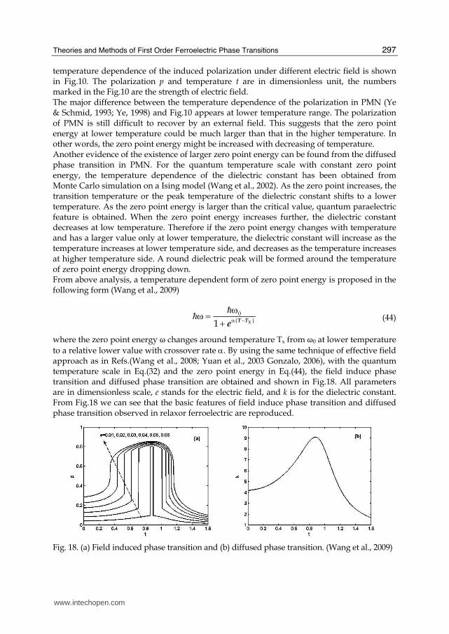
to a relative lower value with crossover rate α. By using the same technique of effective field approach as in Refs.(Wang et al., 2008; Yuan et al., 2003 Gonzalo, 2006), with the quantum temperature scale in Eq.(32) and the zero point energy in Eq.(44), the field induce phase transition and diffused phase transition are obtained and shown in Fig.18. All parameters are in dimensionless scale, e stands for the electric field, and k is for the dielectric constant. From Fig.18 we can see that the basic features of field induce phase transition and diffused phase transition observed in relaxor ferroelectric are reproduced.

Fig. 18. (a) Field induced phase transition and (b) diffused phase transition. (Wang et al., 2009)

www.intechopen.com

Ferroelectrics

298

The dimensionless quantum temperature scale used in Fig.18 is shown in Fig.19. The solid line represents the quantum temperature scale, and the dashed line is for the real temperature scale. The phase transition temperature is marked by the arrow. That means that the state evolution of relaxor ferroelectric misses the phase transition temperature as the temperature decreases, and re-entry of the paraelectric state. The kind of non-ergodic behavior is schematically shown in Fig.19(b) for better understanding.

Fig. 19. (a) Quantum temperature scale and (b) non-ergodic behavior. (Wang et al., 2009)

Overall, relaxor ferroelectrics like PMN are in a tri-critical state of long range ferroelectric order, thermal fluctuations and quantum fluctuations. This critical state can be described by a quantum temperature scale. Following features can be understood from this issue: diffuse phase transition, field induced phase transition, long relaxation time, as well as super-paraelectric state, micro-macro-domain crossover and nonergodic behavior. However, a more adequate expression of temperature dependence of zero point energy is still needed for better description of the physical behavior in the relaxor ferroelectrics.

6. Final remarks

Theoretical methods and models for studying ferroelectric with first order phase transition are definitely not limited to the contents in this chapter. Hopefully results from these theoretical techniques can provide useful information for understanding experimental observations. Heavy-computer relying methods, such as first-principle calculations and molecular dynamic simulations etc, have been applied to investigate the physical properties of ferroelectrics. However, fully understanding of the origin of ferroelectrics might need more efforts from both theoretical and experimental side.

7. References

Ali, R.A.; Wang, C.L.; Yuan, M.; Wang, Y. X. & Zhong, W. L. (2004). Compositional dependence of the Curie temperature in mixed ferroelectrics: effective field approach. Solid State Commun., 129, 365 -367

Arago, C.; Garcia, J.; Gonzalo, J. A.; Wang, C. L.; Zhong, W. L. & Xue, X. Y. (2004). Influence of quantum zero point energy on the ferroelectric behavior of isomorphous systems. Ferroelectrics, 301, 113 -119

www.intechopen.com


299

Aragó, C.; Wang, C. L. & Gonzalo, J. A. (2006). Deviations from Vegard’s law in the Curie temperature of mixed ferroelectric solid solutions. Ferroelectrics, 337, 233-237

Binder, K. (1984). Applications of Monte Carlo Method in Statistical Physics, 2nd Edition, Springer-Verlag, ISBN 038712764X, Berlin

Blinc, R. & Zeks, B. (1974). Soft modes in ferroelectrics and antiferroeletrics, North-Holland Publishing Company, ISBN 0 7204 1462 8, Amsterdam

Bokov, A. A. & Ye, Z. G. (2006). Recent progress in relaxor ferroelectrics with perovskite structure. Journal of Materials Science, 41, 31-52

Chen, H. W.; Yang, C.R.; Zhang, J.H.; Pei, Y.F. & Zhao, Z. (2009). Microstructure and antiferroelectric-like behavior of PbxSr1−xTiO3 ceramics. J Alloys and Compounds, 486, 615-620

Gonzalo, J. A. (1989). Quantum effects and competing interactions in crystals of the mixed rubidium and ammonium dihydrogen phosphate systems. Phys. Rev. B, 39, 12297-12299

Gonzalo, J. A.; Ramírez, R.; Lifante, G. & Koralewski, M. (1993). Dielectric discontinuities and multipolar interactions in ferroelectric perovskites, Ferroelectrics Letters Section, 15, 9-16

Gonzalo, J. A. (2006). Effective Field Approach to Phase Transitions and Some Applications to Ferroelectrics, World Scientific Press, ISBN 981-256-875-1, Singapore

Gonzalo, J. A. & Wang, C. L. (2008). Monte Carlo approach to Phase Transitions, Asociacion Espanola Ciencia y Cultura, ISBN 978-84-936537-9-8，Madrid

Jiang, Q. & Tao, Y. M. (2005). Critical line between the first-order and the second-order phase transition for ferroelectric thin films described by TIM. Phys. Lett. A, 336, 216-222

Kutnjak, Z.; Petzelt, J. & Blinc, R. (2006). The giant electromechanical response in ferroelectric relaxors as a critical phenomenon. Nature, 441, 956-959

Lines, M. E. & Glass A. M. (1997). Principles and Applications of Ferroelectrics and Related Materials, Clarendon Press, ISBN 0 19 851286 4, Oxford

Noheda, B.; Lifante, G. & Gonzalo, J.A. (1993). Specific heat and quadrupole interactions in uniaxial ferroelectrics, Ferroelectrics Letters Section, 15 , 109-114

Noheda, B.; Koralewski, M.; Lifante, G. & Gonzalo J. A. (1994). Dielectric discontinuities and multipolar interactions in ferroelectric perovskites, Ferroelectrics Letters Section, 17, 25-31

Qu, B. D.; Zhong, W. L. & Zhang, P. L. (1997). Ferroelectric superlattice with first-order phase transition. Ferroelectrics, 197, 23-26

Song, T. K.; Kim, J. S.; Kim, M.H.; Lim, W.; Kim, Y. S. & Lee, J. C. (2003). Landau-Khalatnikov simulations for the effects of external streese on the ferroelectric properties of Pb(Zr,Ti)O3 thin films. Thin Soild Films, 424, 84 -87

Teng, B. H. & Sy, H. K. (2005). Transition regions in the parameter space based on the transverse Ising model with a four-spin interaction. Europhys. Lett., 72, 823-829

Wang, C. L.; Qin, Z. K. & Lin, D. L. (1989). First order phase transition in order-disorder ferroelectrics. Phys. Rev. B, 40, 680-685

Wang, C. L.; Zhang, L.; Zhong, W. L. & Zhang, P.L. (1999). Switching characters of asymmetric ferroelectric films. Physics Letters A, 254, 297-300

www.intechopen.com

Ferroelectrics

300

Wang, C. L.; Garcia, J.; Arago, C., Gonzalo, J. A. & Marques, M. I. (2002). Monte Carlo simulation of quantum effects in ferroelectric phase transitions with increasing zero-point energy, Physica A, 312, 181-186

Wang, C. L.; Li, J.C.; Zhao, M.L.; Zhang, J.L.; Zhong, W.L.; Aragó, C.; Marqués, M.I. & Gonzalo, J.A. (2008). Electric field induced phase transition in first order ferroelectrics with large zero point energy. Physica A, 387, 115-122

Wang, C. L.; Li, J. C.; Zhao, M. L.; Liu, J. & Zhang, J. L. (2009). Ferroelectric relaxor as a critical state. Science in China Series E: Technological Sciences, 52, 123-126

Wang, C. L.; Li, J.C.; Zhao, M. L.; Marqués, M.I.; Aragó, C. & Gonzalo, J. A. (2010). Monte Carlo simulation of first order phase transitions, Ferroelectrics, (in press)

Wang, X. S.; Wang, C. L. & Zhong, W. L. (2002). First-order phase transition in ferroelectric superlattice described by the transverse Ising model. Solid State Commun. 122, 311-315

Wang, Y. G.; Zhong, W. L. & Zhang, P. L. (1996). Surface effects and size effects on ferroelectrics with a first-order phase transition. Phys. Rev. B, 53, 11439-11443

Wesselinowa, J. M. (2002). Properties of ferroelectric thin films with a first order phase transitions. Solid State Commun., 121, 89-92

Ye, Z. G. & Schmid, H. (1993). Optical, Dielectric and Polarization Studies of the Electric Field-Induced Phase Transition in Pb(Mg1/3Nb2/3)O3 [PMN] Ferroelectrics, 145, 83-108

Ye, Z. G. (1998). Relaxor Ferroelectric Complex Perovskites: Structure, Properties and Phase Transition, Key Engineering Materials, 155-156, 81-122

Yuan, M.; Wang, C. L.; Wang, Y. X.; Ali, R. A. & Zhang, J. L. (2003). Effect of zero-point energy on the dielectric behavior of strontium titanate. Solid State Commun., 127, 419-421

www.intechopen.com

FerroelectricsEdited by Dr Indrani Coondoo

ISBN 978-953-307-439-9Hard cover, 450 pagesPublisher InTechPublished online 14, December, 2010Published in print edition December, 2010

InTech EuropeUniversity Campus STeP Ri Slavka Krautzeka 83/A 51000 Rijeka, Croatia Phone: +385 (51) 770 447 Fax: +385 (51) 686 166www.intechopen.com

InTech ChinaUnit 405, Office Block, Hotel Equatorial Shanghai No.65, Yan An Road (West), Shanghai, 200040, China

Phone: +86-21-62489820 Fax: +86-21-62489821

Ferroelectric materials exhibit a wide spectrum of functional properties, including switchable polarization,piezoelectricity, high non-linear optical activity, pyroelectricity, and non-linear dielectric behaviour. Theseproperties are crucial for application in electronic devices such as sensors, microactuators, infrared detectors,microwave phase filters and, non-volatile memories. This unique combination of properties of ferroelectricmaterials has attracted researchers and engineers for a long time. This book reviews a wide range of diversetopics related to the phenomenon of ferroelectricity (in the bulk as well as thin film form) and provides a forumfor scientists, engineers, and students working in this field. The present book containing 24 chapters is a resultof contributions of experts from international scientific community working in different aspects of ferroelectricityrelated to experimental and theoretical work aimed at the understanding of ferroelectricity and their utilizationin devices. It provides an up-to-date insightful coverage to the recent advances in the synthesis,characterization, functional properties and potential device applications in specialized areas.

How to referenceIn order to correctly reference this scholarly work, feel free to copy and paste the following:

Chunlei Wang (2010). Theories and Methods of First Order Ferroelectric Phase Transitions, Ferroelectrics, DrIndrani Coondoo (Ed.), ISBN: 978-953-307-439-9, InTech, Available from:http://www.intechopen.com/books/ferroelectrics/theories-and-methods-of-first-order-ferroelectric-phase-transitions

Documents

Theories and Methods of First Order Ferroelectric Phase ...cdn.intechweb.org/pdfs/12502.pdf · barium titanate, lead zirconium titanate, ... kind of theory is often called Landau