Théorie des grandes déviations: Des mathématiques à la ...cermics.enpc.fr/cermics-seminaires/seminaires/cermics/ldt-cermics1.pdf · The generator of the Markovian process defined

Theorie des grandes deviations:Des mathematiques a la physique

Hugo Touchette

National Institute for Theoretical Physics (NITheP)Stellenbosch, Afrique du Sud

CERMICS, Ecole des PontsParis, France

30 novembre 2015

Hugo Touchette (NITheP) Grandes deviations Novembre 2015 1 / 22

Plan

Themes• Typical states

• Fluctuations around typicality

• Many components

Outline• A bit of history

• Basics of large deviations

• Equilibrium systems

• Nonequilibrium systems

......

Lewis (80s) Ellis (1984)Graham (80s)

Gartner (1977)

Freidlin-Wentzell (70s)Lanford (1973)

Donsker-Varadhan (70s)

Sanov (1957)Onsager (1953)

Cramer (1938)

Einstein (1910)

Boltzmann (1877)


Boltzmann (1877)

En

erg

yle

vels

j... — — — — —4 — — — —• —3 — — — — · · · —•2 — —• —• — —1 —• — — — —

1 2 3 4 · · · NParticles i

• Energy distribution:

wj = # particles in level j

• Multinomial distribution:

lnN!∏j wj !

≈ −N∑j

wj lnwj = Ns(w)

• P(w) ≈ eNs(w)


Einstein (1910)

• Generalize Boltzmann

• Macrostate: MN

• Density of states (complexion):

W (m) = # microstates with MN = m

Einstein’s postulate

W (m) = eNs(m)

• Probability:

P(m) = eN[s(m)−s(m∗)]

• Equilibrium: s(m∗) is max


Cramer (1938)

• Sample mean:

Sn =1

n

n∑i=1

Xi , Xi ∼ p(x) IID

• Cumulant:

λ(k) = lnE [ekX ] =

∫Rp(x) ekx dx

• Probability density:

P(Sn = s) = e−nI (s) 1√n

(b0 +

b1

n+ · · ·

)• Rate function:

I (s) = maxk∈Rks − λ(k)

Harald Cramer (1893-1985)


Sanov (1957)

• Sequence of IID RVs:

X1,X2, . . . ,Xn Xi ∼ p(x)

• Empirical distribution:

Ln(x) =1

n

n∑i=1

δXi ,x

P(Ln = ρ) ≈ e−nD(ρ||p)

• Relative entropy:

D(ρ||p) =

∫dx ρ(x) ln

ρ(x)

p(x)

• Law of Large Numbers: Ln → ρ

(1919-1968)

Ivan Nikolaevich Sanov (1919-1968)


Large deviation theory

• Random variable: An

• Probability density: P(An = a)

Large deviation principle (LDP)

P(An = a) ≈ e−nI (a)

• Meaning of ≈:lnP(a) = −nI (a) + o(n)

limn→∞

−1

nlnP(a) = I (a)

• Rate function: I (a) ≥ 0

Goals of large deviation theory

1 Prove that a large deviation principle exists

2 Calculate the rate function


Varadhan’s Theorem

• LDP:P(An = a) ≈ e−nI (a)

• Exponential expectation:

E [enf (An)] =

∫enf (a) P(An = a) da

• Limit functional:

λ(f ) = limn→∞

1

nlnE [enf (An)]

S. R. Srinivasa Varadhan

Abel Prize 2007

Theorem: Varadhan (1966)

λ(f ) = maxaf (a)− I (a)

Special case: f (a) = ka

λ(k) = maxaka− I (a)


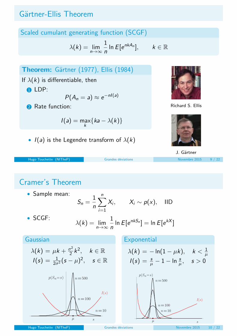
Gartner-Ellis Theorem

Scaled cumulant generating function (SCGF)

λ(k) = limn→∞

1

nlnE [enkAn ], k ∈ R

Theorem: Gartner (1977), Ellis (1984)

If λ(k) is differentiable, then

1 LDP:P(An = a) ≈ e−nI (a)

2 Rate function:

I (a) = maxkka− λ(k)

• I (a) is the Legendre transform of λ(k)

Richard S. Ellis

J. Gartner


Cramer’s Theorem

• Sample mean:

Sn =1

n

n∑i=1

Xi , Xi ∼ p(x), IID

• SCGF:λ(k) = lim

n→∞

1

nlnE [enkSn ] = lnE [ekX ]

Gaussian

λ(k) = µk + σ2

2 k2, k ∈ RI (s) = 1

2σ2 (s − µ)2, s ∈ R

p(S =s)

I(s)

n

s

n=10

n=100

n=500

µ

Exponential

λ(k) = − ln(1− µk), k < 1µ

I (s) = sµ − 1− ln s

µ , s > 0

I(s)

s

n=10

n=100

n=500

µ

p(S =s)n


Sanov’s Theorem

• n IID random variables:

ω = ω1, ω2, . . . , ωn, P(ωi = j) = pj

• Empirical frequencies:

Ln,j =1

n

n∑i=1

δωi ,j =# (ωi = j)

n, Ln = (Ln,1, Ln,2, . . .)

Gartner-Ellis• SCGF:

λ(k) = limn→∞

1

nlnE [enk·Ln ] = ln

q∑j=1

pj ekj

• Rate function:

D(µ) = infkk · µ− λ(k) =

q∑j=1

µj lnµjpj


Beyond IID

Markov processes

XtTt=0

AT = 1T

∫ T0 f (Xt) dt

• P(AT = a) ≈ e−TI (a)

• Long time limit

• Donsker & Varadhan (1975)

SDEs

x(t) = f (x(t)) +√ε ξ(t)

• P[x ] ≈ e−I [x]/ε

• Low noise limit

• Freidlin & Wentzell (1970s)

• Onsager & Machlup (1953)

Applications

• Noisy dynamical systems

• Interacting SDEs

• Stochastic PDEs

• Interacting particle systems

• RWs random environments

• Queueing theory

• Statistics, estimation

• Information theory


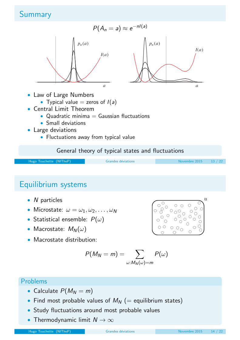
Summary

P(An = a) ≈ e−nI (a)

I(a)

a a

I(a)

p (a)n p (a)n

• Law of Large Numbers• Typical value = zeros of I (a)

• Central Limit Theorem• Quadratic minima = Gaussian fluctuations• Small deviations

• Large deviations• Fluctuations away from typical value

General theory of typical states and fluctuations


Equilibrium systems

• N particles

• Microstate: ω = ω1, ω2, . . . , ωN

• Statistical ensemble: P(ω)

• Macrostate: MN(ω)

u

• Macrostate distribution:

P(MN = m) =∑

ω:MN(ω)=m

P(ω)

Problems

• Calculate P(MN = m)

• Find most probable values of MN (= equilibrium states)

• Study fluctuations around most probable values

• Thermodynamic limit N →∞Hugo Touchette (NITheP) Grandes deviations Novembre 2015 14 / 22

Equilibrium large deviations

MicrocanonicalEinstein (1910)

u

Pu(MN = m) = eS(u,m)/kB

• Extensivity: S ∼ N

• LDP:

Pu(MN = m) ≈ e−NIu(m)

CanonicalLandau (1937)

T

Pβ(MN = m) = e−F (β,m)

• Extensivity: F ∼ N

• LDP:

Pβ(MN = m) ≈ e−NIβ(m)

• Exponential concentration of probability

• Equilibrium states = minima and zeros of I


Maxwell distribution

v

ρ(v

)

• Velocity distribution:

LN(v) =# particles with vi ∈ [v , v + ∆v ]

N∆v

Sanov’s Theorem

Pu(LN = ρ) ≈ e−NIu(ρ)

• Equilibrium distribution:

ρ∗(v) = c v2e− mv2

2kBT


Entropy and free energy

• Density of states:

Ω(u) = # ω with U/N = u

• Large deviation form: Ω(u) ≈ eNs(u)

u

Gartner-Ellis Theorem

s(u) = minββu − ϕ(β)

• Free energy:

ϕ(β) = limN→∞

− 1

NlnZ (β), Z (β) =

∫dω e−βU(ω)

• Z (β) = partition function = generating function

• ϕ(β) = free energy = SCGF

• Basis of Legendre transform in thermodynamics


Sources and applications

• Finite-range systemsLanford (1973)

• Spin systemsEllis (1980s)

• Bose condensationLewis (1980s)

• 2D turbulence

• Long-range systems

• Quantum systemsLenci, Lebowitz (2000)

• Spin glasses

• Large deviation structure

• Typical states and fluctuations

Oscar Lanford III (1940-2013)

John T. Lewis (1932-2004)


Nonequilibrium systems

• Process: Xt

• One or many particles• Markov process• External forces• Boundary reservoirs

• Trajectory: xtTt=0

• Path distribution: P[x ]

• Observable: AN,T [x ]

Ta Tb

J

Problems

• Calculate P(AN,T = a)

• Find most probable values of AN,T (= stationary states)

• Study fluctuations around typical values

• Scaling limits:

N →∞ T →∞ noise→ 0


Example: Pulled Brownian particle

• Glass bead in water

• Laser tweezers

• Langevin dynamics:

mx(t) = −αx︸︷︷︸drag

−k[x(t)− vt]︸︷︷︸spring force

+ ξ(t)︸︷︷︸noise

• Fluctuating work:

WT︸︷︷︸work

= ∆U︸︷︷︸potential

+ QT︸︷︷︸heat T

vtQ

U

LDP

P(WT = w) ≈ e−TI (w)

Fluctuation relation

P(WT = w)

P(WT = −w)= eTcw


Applications

• Driven nonequilibrium systems

• Interacting particle models• Current, density fluctuations• Macroscopic, hydrodynamic limit

• Thermal activation• Kramers escape problem

• Disorded systems

• Multifractals

• Chaotic systems

• Quantum systems

Ta Tb

J

56 H. Touchette / Physics Reports 478 (2009) 1–69

a b

Fig. 20. (a) Exclusion process on the lattice Zn and (b) rescaled lattice Zn/n. A particle can jump to an empty site (black arrow) but not to an occupied site(red arrow). The thin line at the bottom indicates the periodic boundary condition (0) = (1).

interest for these models comes from the fact that their macroscopic or hydrodynamic behavior can be determined fromtheir ‘‘microscopic’’ dynamics, sometimes in an exact way. Moreover, the typicality of the hydrodynamic behavior canbe studied by deriving large deviation principles which characterize the probability of observing deviations in time fromthe hydrodynamic evolution [164]. The interpretation of these large deviation principles follows the Freidlin–Wentzelltheory, in that a deterministic dynamical behavior—here the hydrodynamic behavior—arises as the global minimum andzero of a given (functional) rate function. From this point of view, the hydrodynamic equations, which are the equations ofmotion describing the hydrodynamic behavior, can be characterized as the solutions of a variational principle similar to theminimum dissipation principle of Onsager [214].

Two excellent review papers [113,215] have appeared recently on interacting particle models and their large deviations,so we will not review this subject in detail here. The next example illustrates in the simplest way possible the gist ofthe results that are typically obtained when studying these models. The example follows the work of Kipnis, Olla andVaradhan [216],whowere the first to apply large deviation theory for studying the hydrodynamic limit of interacting particlemodels.

Example 6.11 (Simple Symmetric Exclusion Process). Consider a system of k particles moving on the lattice Zn of integersranging from 0 to n, n > k; see Fig. 20(a). The rules that determine the evolution of the particles are assumed to be thefollowing:

• A particle at site iwaits for a random exponential time with mean 1, then selects one of its neighbors j at random.• The particle at i jumps to j if j is unoccupied; if j is occupied, then the particle stays at i and goes to a waiting period again

before choosing another neighbor to jump to (exclusion principle).

We denote by t(i) the occupation of the ‘‘site’’ i 2 Zn at time t , and by t = (t(0), t(1), . . . , t(n 1)) the wholeconfiguration ormicrostate of the system. Because of the exclusion principle, t(i) 2 0, 1. Moreover, we impose boundaryconditions on the lattice by identifying the first and last site.

The generator of the Markovian process defined by the rules above can be written explicitly by noting that there can bea jump from i to j only if (i) = 1 and (j) = 0. Therefore,

(Lf )() = 12

X

|ij|=1

(i)[1 (j)][f (i,j) f ()], (276)

where f is any function of , and i,j is the configuration obtained after one jump, that is, the configuration obtained byexchanging the occupied state at i with the unoccupied state at j:

i,j(k) =(

(i) if k = j(j) if k = i(k) otherwise.

(277)

To obtain a hydrodynamic description of this dynamics, we rescale the lattice spacing by a factor 1/n, as shown in Fig. 20(b),and take the limit n ! 1 with r = k/n, the density of particles, fixed. Furthermore, we speed-up the time t by a factorn2 to overcome the fact that the diffusion dynamics of the particle system ‘‘slows’’ down as n ! 1. In this limit, it can beproved that the empirical density of the rescaled dynamics, defined by

nt (x) = 1

n

X

i2Zn

n2t(i) (x i/n), (278)

where x is a point of the unit circle C , weakly converges in probability to a field t(x) which evolves on C according to thediffusion equation

@tt(x) = @xxt(x). (279)

It can also be proved that the fluctuations of nt (x) around the deterministic field t(x) follows a large deviation principle,

expressed heuristically as

Pn[nt = t ] = Pn(n

t (x) = t(x)t=0) enI[t ]. (280)

x

F(x

)

∆F

• Exponentially rare fluctuations

• Exponential concentration of typical states

• Same theory for equilibrium and nonequilibrium systems


Summary

• Random variables — ensembles — stochastic systems• Most probable values — equilibrium states — typical states• Fluctuations — rare events• Rate function = entropy• Cumulant function = free energy• Scaling limit: N →∞, T →∞, ε→ 0• Unified language for statistical mechanics

H. TouchetteThe large deviation approach to statistical mechanicsPhysics Reports 478, 1-69, 2009

www.physics.sun.ac.za/~htouchette

Prochain expose

• Markov processes conditioned on large deviations

• When a fluctuation happens, how does it happen?


Documents

Théorie des grandes déviations: Des mathématiques à la ...cermics.enpc.fr/cermics-seminaires/seminaires/cermics/ldt-cermics1.pdf · The generator of the Markovian process defined