Theoretical Foundations of Spatially-Variant Mathematical ...nbouayna/PAMI1.pdf · Theoretical Foundations of Spatially-Variant Mathematical Morphology Part I: Binary Images Nidhal

1

Theoretical Foundations of Spatially-Variant

Mathematical Morphology Part I: Binary

Images

Nidhal Bouaynaya, Student Member, IEEE, Mohammed Charif-Chefchaouni

and Dan Schonfeld, Senior Member, IEEE

Abstract

We develop a general theory of spatially-variant (SV) mathematical morphology for binary images in

the Euclidean space. The basic SV morphological operators (i.e., SV erosion, SV dilation, SV opening and

SV closing) are defined. We demonstrate the ubiquity of SV morphological operators by providing a SV

kernel representation of increasing operators. The latter representation is a generalization of Matheron’s

representation theorem of increasing and translation-invariant operators. The SV kernel representation

is redundant, in the sense that a smaller subset of the SV kernel is sufficient for the representation of

increasing operators. We provide sufficient conditions for the existence of the basis representation in terms

of upper-semi-continuity in the hit-or-miss topology. The latter basis representation is a generalization of

Maragos’ basis representation for increasing and translation-invariant operators. Moreover, we investigate

the upper-semi-continuity property of the basic SV morphological operators. Several examples are used to

demonstrate that the theory of spatially-variant mathematical morphology provides a general framework

for the unification of various morphological schemes based on spatially-variant geometrical structuring

elements (e.g., circular, affine and motion morphology). Simulation results illustrate the theory of the

proposed spatially-variant morphological framework and show its potential power in various image

processing applications.

Index Terms

N. Bouaynaya was with the Department of Electrical and Computer Engineering, University of Illinois at Chicago, Chicago,

IL 60607, USA. She is now with the Department of Systems Engineering, University of Arkansas at Little Rock, Little Rock,

Arkansas 72204, USA (e-mail: [email protected]). D. Schonfeld is with the University of Illinois at Chicago, Chicago, IL

60607, USA (e-mail: [email protected]). M. Charif-Chefchaouni is with the Institut National des Postes et Telecommunications,

Rabat, Morocco (e-mail: [email protected]).

DRAFT

Digital Object Indentifier 10.1109/TPAMI.2007.70754 0162-8828/$25.00 © 2007 IEEE

IEEE TRANSACTIONS ON PATTERN ANALYSIS AND MACHINE INTELLIGENCEThis article has been accepted for publication in a future issue of this journal, but has not been fully edited. Content may change prior to final publication.

2

mathematical morphology, spatially-variant morphology, adaptive morphology, circular morphology,

affine morphology, median filter, kernel representation, basis representation, upper-semi-continuity, hit-

or-miss transform.

I. INTRODUCTION

Since it was first developed in the 1970’s by Matheron [46] and Serra [53], mathematical morphology

emerged as a powerful tool in signal and image processing applications [25], [41], [43], [44]. Mathematical

morphology uses concepts from set theory, geometry and topology to analyze geometrical structures

in signals and images. It introduces the concept of structuring element (SE), which is a geometrical

pattern used to probe the input image. The theory has been used in a wide range of applications

including biomedical image processing [21], [1], shape analysis [31], coding and compression [34], [42],

automated industrial inspection [19], texture analysis [22], [60], radar imagery [30], and multiresolution

techniques and scale-spaces [26], [27], [49]. Morphological operators have been efficiently implemented

in numerous commercial softwares products and computer architectures for digital signal and image

processing applications [23]. The ubiquity of morphological operators has been captured by Matheron’s

kernel representation theorem which asserts that any increasing and translation-invariant operator can

be exactly represented in terms of elementary morphological operators (i.e., morphological erosions and

dilations) using a collection of structuring elements in their kernel (i.e. a set of structuring elements

that characterizes the operator) [46]. Maragos, in his doctoral thesis [37], [39], has provided sufficient

conditions under which the increasing and translation-invariant operators have basis representations.

Initially, the focus of mathematical morphology was devoted to translation-invariant operators (i.e., the

structuring element remains fixed in the entire space). However, the translation-invariance assumption

is not appropriate in many applications. One of the earliest examples of adaptive (or spatially-variant)

structuring elements is given by Beucher et al. [5] in the analysis of images from traffic control cameras.

Because of the perspective effect, vehicles at the bottom of the image are closer and appear larger than

those higher in the image. Hence, the structuring element (SE) should follow a law of perspective, e.g.,

vary linearly with its vertical position in the image. In range imagery techniques, the grayscale value of

each pixel is proportional to its distance to the imaging device. Hence, the apparent length of a feature in

such images is a function of its gray value range. One can therefore process (e.g., extract or eliminate) all

the differently scaled instances of the object of interest by adapting the structuring element to the local

range. Verly and Delanoy [58] developed an algorithm to design and apply adaptive structuring elements

for object extraction in range images. The need for spatially-variant morphological image processing

DRAFT


3

arises even in the most basic applications in image processing, namely image smoothing and denoising.

In morphological image denoising, there is a tradeoff between noise removal and detail preservation

in the image. Moreover, translation-invariant morphological filters are inherently incapable of restoring

image structures that are smaller than the structuring element used [18], [43], [44], [52]. Thus, some

geometric information of the image may be lost while reducing the noise. Many researchers proposed

different adaptive smoothing algorithms, which consist of removing noise while preserving image features

by adapting the structuring elements to local features of the image. We cite, in chronological order, some

application-oriented algorithms for adaptive morphological denoising and smoothing. Morales [47] used

a SE that changes adaptively according to the variance of the input signal in order to remove artifacts

and noise from images. In [12], a family of SEs, which is closed under translation, is used to efficiently

implement the maximum opening filter. The size of the SE is determined by the image characteristics

and the noise patterns. This method allows for the elimination of more impulsive noise without blurring

the edges compared to the conventional translation-invariant maximum opening filter. In [10], the SE

changes with respect to the edge strength of the signal. That is, the line SE is shorter for a strong edge

and longer for a weak one. So, the edges are not blurred by this method much as they are blurred by

a conventional fixed SE. Chen et al [11] developed the progressive umbra-filling (PUF) algorithm for

adaptive signal smoothing. Their algorithm gradually fills the umbra of a signal with a set of overlapping

SEs that vary from larger to smaller in scale. The PUF algorithm is shown to successfully reduce the

bumping noise without oversmoothing the signal. In [45], a locally adaptive structuring element is used for

contour extraction in ultrasound images corrupted by speckle noise. In [56], adaptive elliptical structuring

elements were used in a morphological edge linking algorithm, where the size and orientation of the SE

is adjusted according to the local properties of the image, such as slope and curvature. Based on distance

transformation, Cuisenaire [14] developed efficient algorithms for the implementation of the adaptive

erosion, dilation, opening and closing using ball structuring elements of varying sizes. Debayle et al. [15],

[16] used the concept of Adaptive Neighborhood (AN) that was proposed by Gordon and Rangayyan

[20] to define AN-based structuring elements. The latter SEs depend on a morphological or geometrical

criterion with a homogeneity tolerance so as to take into account the local features of the image. Lerallut

et al. [36] proposed amoeba structuring elements, which adapt their size and shape to the content of the

image.

Adaptive mathematical morphology for shape representation and image decomposition has been scarcely

investigated. In [57], an adaptive decomposition of binary images into a number of simple shapes based on

homothetics of a set of structuring elements was proposed in order to minimize the number of points in the

DRAFT


4

representation of the image. In [61], eight structuring elements were used to generalize the morphological

skeleton representation. In this representation, the number of points needed to represent a given shape

is significantly lower than that in the standard morphological skeleton transform. In [7], we extended

the morphological skeleton representation framework presented in [51] to the spatially-variant case. We

also provided a practical algorithm to construct the optimal structuring elements, which minimize the

cardinality of the spatially-variant morphological skeleton representation.

The examples cited above clearly illustrate the need to develop a unified spatially-variant mathematical

morphology theory. The objective of this paper is, thus, to present a general theory of spatially-variant

(SV) mathematical morphology in the Euclidean space, which will unify all the techniques proposed

thus far into a comprehensive mathematical framework. The proposed theory preserves the concept of

structuring element, which is crucial in the design of geometrical signal and image processing applications.

This paper is the first in a sequence of two papers (Parts I and II). In this part, we will investigate the

foundations of the theory of spatially-variant mathematical morphology in the Euclidean space for binary

signals and images. The treatment of the graylevel case will be explored in Part II.

This paper is organized as follows: In Section II, we review the previous work related to the extension

of mathematical morphology to transformations that do not commute with the translation operator. In

Section III, we define the basic spatially-variant morphological operators (i.e. SV erosion, SV dilation,

SV opening and SV closing). The properties of the basic SV morphological operators are enumerated in

Appendix A. Subsequently, we provide several examples of non-translation-invariant morphology such as

affine morphology and adaptive neighborhood morphology, which establish our representation as a unified

theory of spatially-variant mathematical morphology. Matheron’s representation theorem is extended to

the spatially-variant case in Section IV. The spatially-variant kernel representation is a powerful theoret-

ical result since it demonstrates the ubiquity of the SV morphological operators by representing every

increasing operator in terms of SV erosions or dilations. However, as was the case in translation-invariant

mathematical morphology [37], the practical importance of the SV kernel representation is limited since

it requires an infinite number of SV erosions or SV dilations to implement the operator. Following the

development of Maragos’ basis representation for translation-invariant operators presented in [2], [17]

and [37], we provide, in Section V, sufficient conditions under which the SV basis representation exists.

These sufficient conditions are expressed in terms of upper-semi-continuity in the hit-or-miss topology.

We subsequently investigate some topological properties of the SV erosion and SV dilation and provide,

as an example, a basis representation of the adaptive median filter. In Section VI, we provide simulation

results to show the power of the SV mathematical morphology theory in image reconstruction, pattern

DRAFT


5

segmentation and shape representation. A summary of the paper and concluding remarks are provided in

Section VII.

II. RELATED WORK

An extension of the theory of mathematical morphology from the Euclidean space to complete lattices

was initiated by Matheron [46] and Serra [54]. Heijmans and Ronse further pursued their work on lattice

morphology in [28] and [29]. Lattice morphology is a powerful tool that provides an abstraction of

mathematical morphology based on lattice theory, a topic devoted to the investigation of the algebraic

properties of partially-ordered sets [6], [25]. The general properties of lattice morphological operators

depend only on the characteristics of the order relation and the supremum and infimum of the complete

lattice. Although lattice morphology is an extremely powerful theory, it relies on abstract mathematical

concepts for the representation of the morphological operators and is, therefore, not accessible to engineers

in the development of signal and image processing systems. In particular, the general theory of lattice

morphology cannot be used to convey the notion of a structuring element, which is critical in the

development of morphological image analysis applications. Thus, it is interesting to focus on special

cases of the general lattice morphology theory, which convey the intuition provided by the translation-

invariant theory of mathematical morphology in the Euclidean space.

Earlier efforts to extend mathematical morphology theory to non-translation-invariant operators while

preserving the notion of the structuring element have been presented in special cases. A generalization

of Euclidean morphology to arbitrary abelian symmetry groups was investigated in [24] and [50]. This

concept provides, for example, for the representation of morphological operators in terms of a family of

circular structuring elements (i.e, rotation and scaling of an elementary SE). Maragos, in [40], extended the

notion of circular morphology by introducing the affine morphology framework. Heijmans and Ronse [28],

[29] characterized morphological operators in complete lattices having a certain type of abelian group of

automorphisms generalizing translations. Subsequently, they extended Matheron’s theorem to increasing

operators that are invariant under the group operator. Roedrink [48] extended Euclidean morphology

by including invariance under more general groups of transformations (not necessarily abelian) such as

the Euclidean motion group, the similarity group, the affine group and the projective group. The most

general representation, in the Euclidean space, was introduced by Serra in [54, Chap.2-4]. He defined

the concept of a structuring function that associates to each point in space a local structuring element.

This representation generalizes all prior efforts in the Euclidean space while preserving the concept of

the structuring element. In his work, Serra uses the basic spatially-variant morphological operators to

DRAFT


6

analyze the notion of connectivity and induced metrics. Chefchaouni and Schonfeld [8], [9] extended

Serra’s work on spatially-variant mathematical morphology and illustrated the concept of a spatially-

variant kernel representation for binary increasing systems.

In this paper, we elaborate on Serra’s and Chefchaouni and Schonfeld’s work on spatially-variant

mathematical morphology, in the Euclidean space, to provide a comprehensive theory of spatially-variant

mathematical morphology, which captures the geometrical interpretation of the structuring element.

The proposed theory is the most general framework of spatially-variant mathematical morphology that

preserves the notion of the structuring element. For example, our approach unifies the work of Heijmans

and Ronse on T -invariant operators, where T is an abelian group of automorphisms of a complete lattice

[28] and the work of Maragos on affine morphology [40]. Through our work, we hope to provide a sound

mathematical foundation to past and future research in spatially-variant morphological signal and image

processing, which captures the geometrical intuition of practitioners in the engineering community.

Throughout the paper, we provide reference to known results and limit the presentation of proofs to

new contributions.

III. SPATIALLY-VARIANT MATHEMATICAL MORPHOLOGY

A. Preliminaries

In this paper, we consider the continuous or discrete Euclidean space E = Rn or Z

n for some n > 0

1. The set P(E) denotes the set of all subsets of E. Elements of the set E will be denoted by lower-case

letters; e.g., a, b, c. Elements of the set P(E) will be denoted by upper-case letters; e.g., A,B,C. An

order on P(E) is imposed by the inclusion ⊆. We use ∪ and ∩ to denote the union and intersection in

P(E), respectively. “ ⇒,⇔,∀,∃” denote, respectively, “implies,” “if and only if (iff)”, “for all” and

“there exist(s)”. Xc denotes the complement of X. The translate of the set X by the element a ∈ E is

defined by X + a = {x + a : x ∈ X}. The cardinality, |X|, of a set X is the total number of elements

contained in the set. X B,X ⊕B denote the translation-invariant erosion and dilation, respectively, of

the set X by the structuring element B. We use O = P(E)P(E) to denote the set of all operators mapping

P(E) into itself. Elements of the set O will be denoted by lower case Greek letters; e.g., α, β, γ. An

order on O is imposed by the inclusion ⊆; i.e., α ⊆ β if and only if α(X) ⊆ β(X) for every X ∈ P(E).

We shall restrict our attention to non-degenerate operators, i.e., ψ(E) = E and ψ(∅) = ∅ for every ψ ∈ O

(the set ∅ ∈ P(E) is used to denote the empty set).

1The work presented in this paper is valid for complete atomic Boolean lattices except in Section V where specific conditions

on the space E will be provided.

DRAFT


7

An operator ψ ∈ O is

• increasing if X ⊆ Y =⇒ ψ(X) ⊆ ψ(Y ) (X,Y ∈ P(E));

• translation-invariant if ψ(X + a) = ψ(X) + a (X ∈ P(E), a ∈ E);

• idempotent if ψ(ψ(X)) = ψ(X) (X ∈ P(E));

• extensive (resp. anti-extensive) if X ⊆ ψ(X) (resp. ψ(X) ⊆ X) (X ∈ P(E)).

The mapping ψ∗ in O is the dual of the mapping ψ in O iff ψ∗(X) = (ψ(Xc))c (X ∈ P(E)).

B. Erosions and Dilations

Consider the spatially-variant structuring element θ given by a mapping from E into P(E). The class of

all such mappings inherits the complete lattice structure of P(E) by setting θ1 ≤ θ2 ⇐⇒ θ1(z) ⊆ θ2(z)

for every z ∈ E. The transposed spatially-variant structuring element θ ′ is given by a mapping from E

into P(E) such that

θ′(y) = {z ∈ E : y ∈ θ(z)} (y ∈ E). (1)

In the translation-invariant case, the mapping θ is the translation operator by a fixed set B, i.e., θ(y) =

B + y, for every y ∈ E. So, z ∈ θ′(y) ⇔ y ∈ θ(z) ⇔ y ∈ (B + z) ⇔ z ∈ (B + y), where B = −B

is the reflected set of B. Hence, the transposed mapping reduces, in the translation-invariant case, to the

translation by the reflected set B. As in the translation-invariant mathematical morphology, the choice of

the structuring element mapping is application oriented.

Definition 1: The spatially-variant erosion Eθ ∈ O is defined as

Eθ(X) = {z ∈ E : θ(z) ⊆ X} =⋂

x∈Xc

θ′c(x) (X ∈ P(E)). (2)

Definition 2: The spatially-variant dilation Dθ ∈ O is defined as

Dθ(X) = {z ∈ E : θ′(z) ∩ X �= ∅} =⋃

x∈X

θ(x) (X ∈ P(E)). (3)

The right hand-side equalities in definitions 2 and 3 can be easily verified and thus their proof will

be omitted. The SV erosion and SV dilation are increasing and form an adjunction. Hence, the basic

properties of translation-invariant erosion and dilation can be transposed to the SV erosion and dilation.

These properties are enumerated in Appendix A.

As in the translation-invariant mathematical morphology, a large class of SV binary operators can be

built from the two basic SV operators. We give here only the spatially-variant version of the morphological

opening and closing operators. The spatially-variant opening γθ is given by

γθ(X) = Dθ(Eθ(X)) =⋃

{θ(y) : θ(y) ⊆ X; y ∈ E}, (4)

DRAFT


8

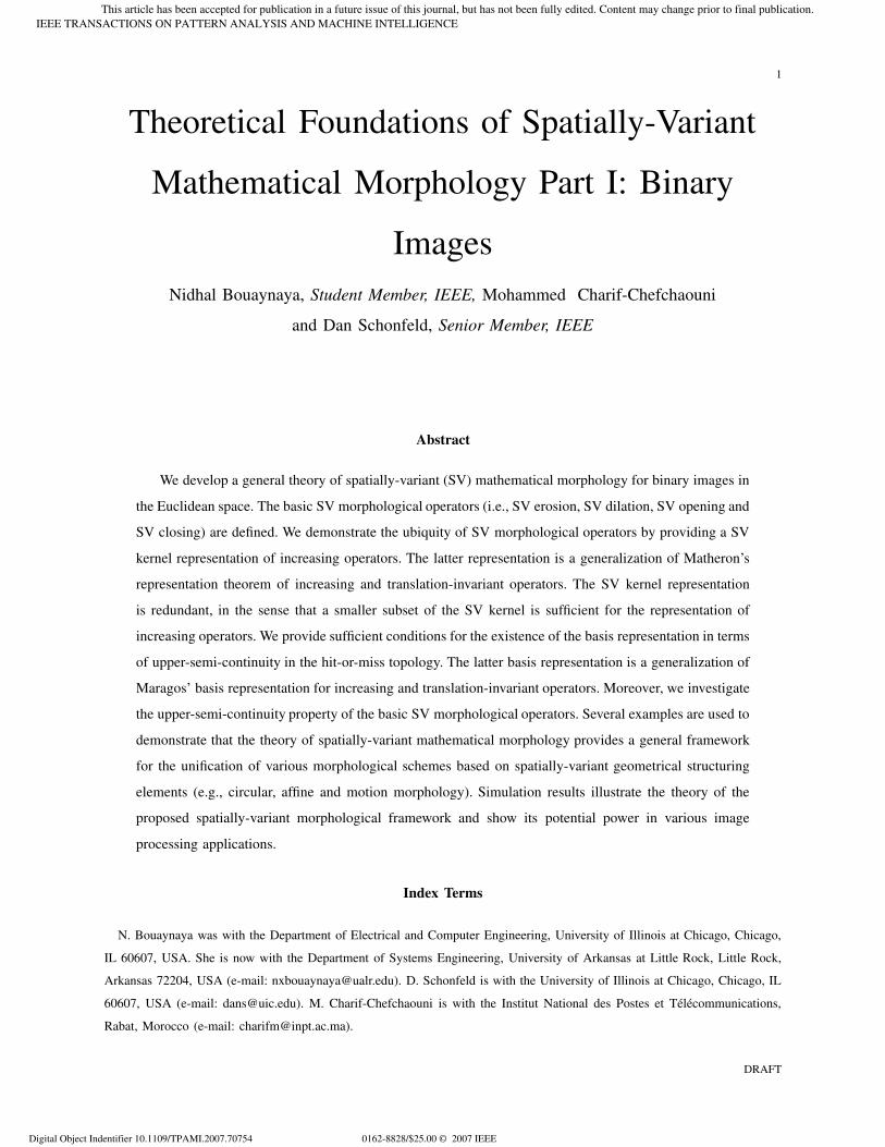
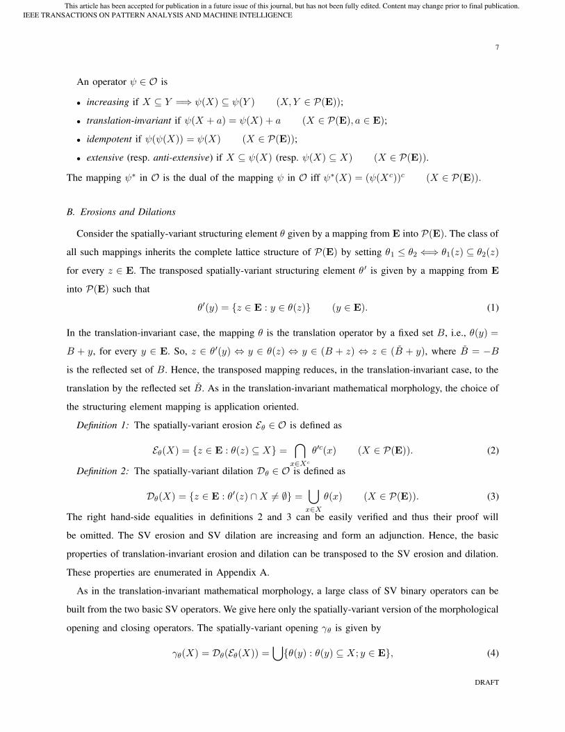
(a) (b) (c) (d)

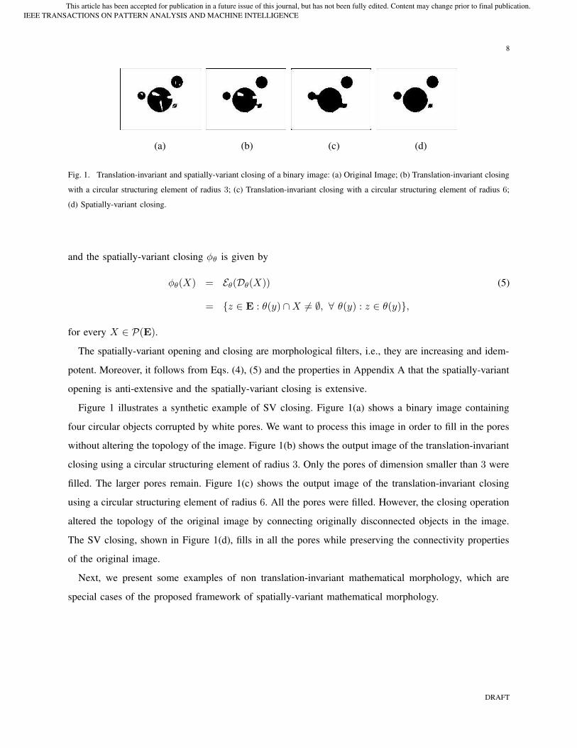
Fig. 1. Translation-invariant and spatially-variant closing of a binary image: (a) Original Image; (b) Translation-invariant closing

with a circular structuring element of radius 3; (c) Translation-invariant closing with a circular structuring element of radius 6;

(d) Spatially-variant closing.

and the spatially-variant closing φθ is given by

φθ(X) = Eθ(Dθ(X)) (5)

= {z ∈ E : θ(y) ∩ X �= ∅, ∀ θ(y) : z ∈ θ(y)},

for every X ∈ P(E).

The spatially-variant opening and closing are morphological filters, i.e., they are increasing and idem-

potent. Moreover, it follows from Eqs. (4), (5) and the properties in Appendix A that the spatially-variant

opening is anti-extensive and the spatially-variant closing is extensive.

Figure 1 illustrates a synthetic example of SV closing. Figure 1(a) shows a binary image containing

four circular objects corrupted by white pores. We want to process this image in order to fill in the pores

without altering the topology of the image. Figure 1(b) shows the output image of the translation-invariant

closing using a circular structuring element of radius 3. Only the pores of dimension smaller than 3 were

filled. The larger pores remain. Figure 1(c) shows the output image of the translation-invariant closing

using a circular structuring element of radius 6. All the pores were filled. However, the closing operation

altered the topology of the original image by connecting originally disconnected objects in the image.

The SV closing, shown in Figure 1(d), fills in all the pores while preserving the connectivity properties

of the original image.

Next, we present some examples of non translation-invariant mathematical morphology, which are

special cases of the proposed framework of spatially-variant mathematical morphology.

DRAFT


9

C. Examples

a) Circular morphology [28]: Consider E = R2 − 0. Let (ra, ϕa) be the polar coordinates of a

given a ∈ E. We define the operation � by

a � b = (rarb, ϕa + ϕb), (a, b ∈ E). (6)

Observe that the operation � on E corresponds to the multiplication in the complex plane if we associate

the complex number r expjϕ to each (r, ϕ) ∈ E. Consider a non empty set A ∈ P(E). Define the

mapping θ as follows

θ(z) = A � z = {a � z : a ∈ A} (z ∈ E). (7)

That is, to each point z ∈ E, the mapping θ associates the scaled and rotated version of the set A by the

magnitude of the point z, rz , and its angle ϕz . Then, θ′(z) = A−1 � z, where A−1 = { 1a

: a ∈ A}. The

SV erosion and dilation defined in (2) and (3), respectively, become

X c A = {z ∈ E : (A � z) ⊆ X} (X ∈ P(E)), (8)

and

X ⊕c A = {z ∈ E : (A−1 � z) ∩ X �= ∅} (X ∈ P(E)). (9)

Equations (8) and (9) are the circular erosion and dilation, respectively, defined in [28]. Therefore, circular

morphology is a special case of the proposed spatially-variant mathematical morphology.

b) Affine morphology [40]: Let E = R2 and let G be the set defined by

G = {(M, t) : M ∈ R2×2, det(M) �= 0, t ∈ R

2}. (10)

Consider a subset S ⊆ G. Define the structuring element mapping θ : E → P(E) as

θ(z) = {Mz + t : (M, t) ∈ S}. (11)

The transposed structuring element is then given by θ ′(z) = {M−1(z− t) : (M, t) ∈ S}. Hence, one can

easily show that the spatially-variant erosion and dilation defined in (2) and (3), respectively, reduce to

X a S =⋂

(M,t)∈S

{M−1(x − t) : x ∈ X}, (12)

and

X ⊕a S =⋃

(M,t)∈S

{Mx + t : x ∈ X}. (13)

DRAFT


10

Equations (12) and (13) are the affine erosion and dilation, respectively, defined in [40]. This establishes

the affine morphology framework as a special case of the spatially-variant morphology theory. Observe

that the affine group is not an abelian group and therefore, the theory of Heijmans and Ronse on T -

invariant operators presented in [28] does not apply.

c) Amoeba morphology [36]: Consider E = Z2. Denote by I(x) the value of the image at position

x. Let d be a distance defined between the values of the image. Let σ = (x = x0, x1, · · · , xn = y) be a

path between the points x and y. Let λ > 0 and r > 0. The length of the path σ is defined as

L(σ) =

n∑i=1

[1 + λ d(I(xi), I(xi+1))]. (14)

The amoeba distance with parameter λ is defined by dλ(x, y) = minσ L(σ). Define the structuring

element mapping θ as

θ(x) = Bλ,r(x) = {y : dλ(x, y) ≤ r}. (15)

Then, the SV erosion and dilation defined in Eqs. (2) and (3), respectively, reduce to

Eθ(X) = {z ∈ E : Bλ,r(z) ⊆ X}, and Dθ(X) =⋃

x∈X

Bλ,r(x). (16)

Equation (16) coincides with the definitions of the amoeba erosion and dilation introduced in [36]. Thus,

amoeba morphology is another special case of the proposed spatially-variant mathematical morphology

framework.

d) Adaptive neighborhood morphology [15], [16]: Consider E = R2. Let h : R

2 → R be a criterion

mapping such as luminance or contrast. Let m > 0. For each x ∈ E, define the connected set V hm(x) by

V hm(x) = {y : |h(y) − h(x)| ≤ m}. Choose the SE mapping θ as follows:

θ(x) =⋃z∈E

{V hm(z) : x ∈ V h

m(z)}. (17)

The SV erosion and dilation defined in Eqs. (2) and (3), respectively, reduce to

Eθ(X) = {z ∈ E : ∃y ∈ E such that z ∈ V hm(y) and V h

m(y) ⊆ X}, (18)

and

Dθ(X) =⋃

x∈X

⋃z∈E

{V hm(z) : x ∈ V h

m(z)}. (19)

Equations (18) and (19) are, respectively, the adaptive neighborhood erosion and dilation presented in [15].

Thus, adaptive neighborhood morphology is yet another special case of the spatially-variant mathematical

morphology theory.

DRAFT


11

The above examples are practical special cases of the proposed theory of spatially-variant mathematical

morphology. Each example corresponds to a special choice of the structuring element mapping θ that is

application oriented. For example, affine signal transformations are useful for modelling self-similarities

in fractal images and shape deformations in visual motion [40]. Circular morphology is useful for circular-

invariant material structure such as radar displays and echographic images [28]. Amoeba morphology

is effective for denoising [36] and adaptive neighborhood morphology was illustrated for multi-scale

representation and segmentation [15].

In the next section, we demonstrate the ubiquity of the basic SV operators, i.e., SV erosion and SV

dilation, by proving that every increasing operator can be exactly represented in terms of SV erosions or

SV dilations.

IV. SPATIALLY-VARIANT KERNEL REPRESENTATION

A. Theoretical Analysis

We extend the concept of the kernel introduced by Matheron, for translation-invariant operators [46],

to the spatially-variant case as follows;

Definition 3: The kernel, Ker(ψ), of a spatially-variant operator ψ ∈ O is given by

Ker(ψ) = {θ : z ∈ ψ(θ(z)), for every z ∈ E}. (20)

The SV kernel of a non-degenerate operator is non-trivial as the following proposition shows;

Proposition 1: Ker (ψ) �= ∅, ∀ψ ∈ O .

An important property of the SV kernel of an increasing operator is that it is unique. Furthermore, the

mapping that associates each operator ψ ∈ O to its kernel is an isomorphism.

Proposition 2: Given two operators ψ1, ψ2 ∈ O, we have ψ1 ⊆ ψ2 if and only if ker (ψ1) ⊆ ker (ψ2).

We now provide the kernel representation of increasing operators based on SV erosions and SV dilations.

Theorem 1: An operator ψ ∈ O is increasing if and only if ψ can be exactly represented as union

of spatially-variant erosions by mappings in its kernel or equivalently as intersection of spatially-variant

dilations by the transposed mappings in the kernel of its dual ψ∗, i.e.,

ψ(X) =⋃

θ∈Ker(ψ)

Eθ(X) =⋂

θ∈Ker(ψ∗)

Dθ′(X), (X ∈ P(E)). (21)

B. Examples

e) Circular morphology [28]: We say that a mapping ψ ∈ O is circular-invariant if for every

X ∈ P(E) and for every z ∈ E, ψ(X � z) = ψ(X) � z. It is straightforward to verify that the union

DRAFT


12

and intersection of circular invariant operators are circular invariant. The following proposition shows

that the circular erosion and dilation, defined in Eqs. (8) and (9), are circular-invariant.

Proposition 3: Given a set A ∈ P(E), the circular erosion and the circular dilation, defined in Eqs.

(8) and (9) respectively, are circular invariant, i.e., for every z ∈ E, we have

(X � z) c A = (X c A) � z, (X ∈ P(E)), (22)

and

(X � z) ⊕c A = (X ⊕c A) � z, (X ∈ P(E)). (23)

Therefore, from Theorem 1 and the kernel representation of group-operators in [25, Theorem 5.35],

every increasing and circular-invariant operator can be exactly represented as union of circular erosions,

or equivalently, as intersection of circular dilations [28].

f) Affine morphology [40]: Let E = R2. Consider the set G defined in Eq. (10), and S ⊂ G.

Define the affine transformation of a set X ∈ P(E) by the pair (A, b) ∈ G as the point by point affine

transformation, i.e., AX + b = {Ax + b : x ∈ X}. We say that an operator ψ ∈ O is affine-invariant

if and only if for every (A, b) ∈ G, ψ(AX + b) = Aψ(X) + b. We show, using a counter example,

that the affine erosion and dilation defined in Eqs. (12) and (13), respectively, are not affine-invariant

operators. Consider the set S = {(I, t)}, where I is the identity matrix and t �= 0. Then, from Eq. (12),

we observe that, for every A �= I , (AX + b) a S = {y − t : y ∈ (AX + b)} = AX + b − t, whereas

A(X a S) + b = A(X − t) + b = AX + b − At. Hence the affine erosion and affine dilation are not

affine-invariant. Nevertheless, Theorem 1 provides a sufficient condition for an operator to be represented

as union of affine erosions; namely, if all the mappings in the kernel of an increasing operator ψ are

of the form given by equation (11), then ψ can be exactly represented as union of affine erosions or

equivalently as intersection of affine dilations.

V. BASIS REPRESENTATION

A. Motivation

The SV kernel representation, given in Eq. (20), is redundant, in the sense that a smaller subset of

the kernel is sufficient for the representation of increasing operators. This can be seen, in the case of

the representation by SV erosions, as follows: if θ1, θ2 ∈ Ker(ψ) are such that θ1 ≤ θ2, then Eθ2⊆ Eθ1

.

Therefore, if the above θ1 and θ2 are contained in the kernel of an increasing operator ψ, its corresponding

kernel representation will be redundant.

In the following proposition, we demonstrate that the kernel of an increasing operator is actually infinite.

DRAFT


13

Proposition 4: Let ψ ∈ O be an increasing operator. Then the kernel of ψ is infinite.

In order to derive minimal representations for increasing operators, we need the notion of a basis of the

kernel, which was first introduced by Maragos [37], [39] for translation-invariant operators.

Definition 4: Let ψ ∈ O be an increasing operator. The basis Bψ of Ker (ψ) is the collection of

minimal kernel mappings, formally defined as

Bψ = {θM ∈ Ker(ψ) : θ ∈ Ker(ψ) and θ ≤ θM =⇒ θ = θM}.

Observe that definition 4 corresponds to the definition of a minimal basis. A more general definition

of the basis as a subcollection of the kernel that is sufficient for representation can be found in [2]. If

the basis of an increasing operator exists, then the kernel representation of the operator reduces to a

representation by the elements of the basis, which will allow in some cases a drastic reduction in the

number of elements in the representation of the operator, as we will show in the examples.

Before proving that increasing and upper-semi-continuous operators have a basis representation, we

briefly recall the definition of upper-semi-continuity in the hit-or-miss topology and study the topological

properties of the SV basic morphological operators. For a comprehensive algebraic and topological

background, we refer the reader to [4], [6], [37], [46], [53].

B. Upper-semi-continuity in the hit-or-miss topology

From now on, E is assumed to be a locally compact, Hausdorff and second countable topological

space. We denote by F the set of all closed subsets of E, by G the set of all open subsets of E and by

K the set of all compact subsets of E. Matheron defined a topology on F called the hit-or-miss topology

[46]. We denote by O′

the set of all operators mapping F into itself. From now on, we consider only

mappings in O′

. In particular, the SV structuring element is now a mapping from E to F .

A mapping ψ in O′

is upper-semi-continuous (u.s.c) if and only if for any K ∈ K, the set ψ−1(FK) is

open in F [46], where FK is the class of the closed sets disjoint of K, i.e., FK = {F : F ∈ F , F ∩K =

∅}. A useful characterization of increasing u.s.c. mappings in F is given by the following proposition

due to Matheron:

Proposition 5: [46] Let ψ be an increasing mapping in O′

. ψ is upper-semi-continuous if and only if

for every sequence {Xn}n∈N of elements of F such that Xn ↓ X in F (i.e., X1 ⊇ X2 ⊇ · · · ⊇ Xn ⊇ · · ·

and X =⋂

n≥1 Xn), we have ψ(Xn) ↓ ψ(X) in F .

Observe that continuity implies upper-semi-continuity but the converse is not true in general [46]. It

is well known that the translation-invariant erosion of a closed set by a compact structuring element

DRAFT


14

is upper-semi-continuous and the translation-invariant dilation of a closed set by a compact structuring

element is continuous [46], [54]. We generalize this result to the spatially-variant case. We say that the

mapping θ is closed (resp. compact) if θ(z) is a closed (resp. compact) set, for every z ∈ E. θ : E → F

(resp. K) is continuous if and only if for every sequence {zn}n∈N ⊂ E converging towards z ∈ E, the

sequence of sets {θ(zn)}n∈N in F (resp. K) converges towards the set θ(z) in F (resp. K) in the sense

of [46, Theorem 1-2-2] (resp. [46, Theorem1-4-1]) and we write θ(xn)F−→ θ(x) (resp. θ(xn)

K−→ θ(x)).

First, we prove that, under specific conditions on the SE mapping, the SV erosion and SV dilation are

mappings from F into itself.

Proposition 6: Consider the SE mapping θ .

a) If θ is continuous from E to F , then F ∈ F ⇒ Eθ(F ) ∈ F ;

b) If θ′ is continuous from E to K, then F ∈ F ⇒ Dθ(F) ∈ F .

Proposition 7: (a) If the mapping θ is continuous from E to F , then the spatially-variant erosion Eθ

is upper-semi-continuous from F to F .

(b) If the mappings θ′ is continuous from E to K, then the spatially-variant dilation is upper-semi-

continuous from F to F .

For a general set mapping ψ, the property of upper-semi-continuity is not easily tractable. We provide

the following easy test for upper-semi-continuity;

Proposition 8: Let ψ1 and ψ2 be two increasing and upper-semi-continuous operators from F to F .

Then their union ψ = ψ1 ∪ ψ2 and their intersection ψ′ = ψ1 ∩ ψ2 are also increasing and upper-semi-

continuous operators from F to F .

An obvious conclusion from Proposition 8 is that any finite union or intersection of increasing and

upper-semi-continuous operators is also increasing and upper-semi-continuous. In particular, if a family

of mappings {θi}i=1,··· ,N and its transpose {θ′i}i=1,··· ,N are continuous from E to K 2, any finite union

or intersection of SV erosions and SV dilations by mappings in {θi}i=1,··· ,N is an upper-semi-continuous

increasing operator from F to F .

C. Spatially-Variant Basis Representation

In order to prove that the SV kernel of an u.s.c. increasing operator has a minimal element, we need

the following lemma;

2If a mapping θ is continuous from E to K, then θ is also continuous from E to F because every compact subset of a

Hausdorff space is closed.

DRAFT


15

Lemma 1: If L is a linearly ordered subset of F , then there exists a sequence {Xn}n∈N of elements

of L such that Xn ↓⋂

L for the hit-or-miss topology defined on F .

Theorem 2: Let ψ ∈ O′

be an increasing operator. If ψ is upper-semi-continuous, then the kernel of

ψ has a minimal element.

We now show that the minimal elements of the kernel are sufficient to represent the increasing and u.s.c.

operator ψ.


be an upper-semi-continuous increasing operator. For every θ ∈ Ker(ψ), there

exists a minimal element θM ∈ Bψ such that θM ≤ θ.

Finally, we provide the representation of an increasing u.s.c. operator by its minimal elements.


be an increasing upper-semi-continuous operator. Then, ψ is exactly repre-

sented as a union of spatially-variant erosions by mappings in its basis Bψ, i.e.,

ψ(X) =⋃

θ∈Bψ

Eθ(X) (X ∈ F). (24)

A minimal representation of an increasing upper-semi-continuous operator as an intersection of SV

dilations is obtained by duality as follows:

Corollary 1: If ψ is increasing from G to G and has an upper-semi-continuous dual ψ∗ from F to

F , then ψ can be exactly represented as an intersection of spatially-variant dilations by the transposed

mappings in the basis of its dual, i.e.,

ψ(X) =⋂

θ∈Bψ∗

Dθ′(X) (X ∈ G). (25)

In the discrete Euclidean space Zn, the set of open sets and closed sets are equivalent to the power set

P(Zn). Therefore, every mapping ψ from F to F has a dual mapping ψ∗ from F to F . Hence, if ψ (resp.,

ψ∗) is increasing and upper-semi-continuous, then the basis representation as union of spatially-variant

erosions (resp. intersection of spatially-variant dilations) exists.

D. Examples

SV erosion: Consider the SV erosion by the continuous SE mapping λ : E → F . Then the smallest

mapping in the kernel of the SV erosion is λ, i.e., BEλ= {λ}.

SV dilation: Consider the SV dilation by the continuous SE mapping λ : E → K. Then the smallest

mappings in the kernel of the SV dilation are the mappings that associate to each point z ∈ E a singleton

{tz}, where tz ∈ λ(z), i.e.,

BDλ= {θ : θ(z) = {tz}, for some tz ∈ λ(z), ∀ z ∈ E}. (26)

DRAFT


16

Thus the SV erosion has only one basis set. If the cardinality of the mapping λ is finite, i.e., |λ(z)| ≤

∨z∈E|λ(z)| = n, then, for each z ∈ E, there are at most n mappings θ satisfying θ(z) = {tz}, for some

tz ∈ λ(z). Define the support of the mapping λ as Spt(λ) = {z ∈ E : λ(z) �= ∅}. If Spt(λ) is infinite,

then there are an infinite number of mappings in the basis of the SV dilation even though λ has a finite

cardinality. If, however, Spt(λ) is finite, then the basis of the SV dilation, by the mapping λ, is finite. In

this case, let N = |Spt(λ)|, then Nn is an upper bound for the number of elements in the basis of the

SV dilation Dλ.

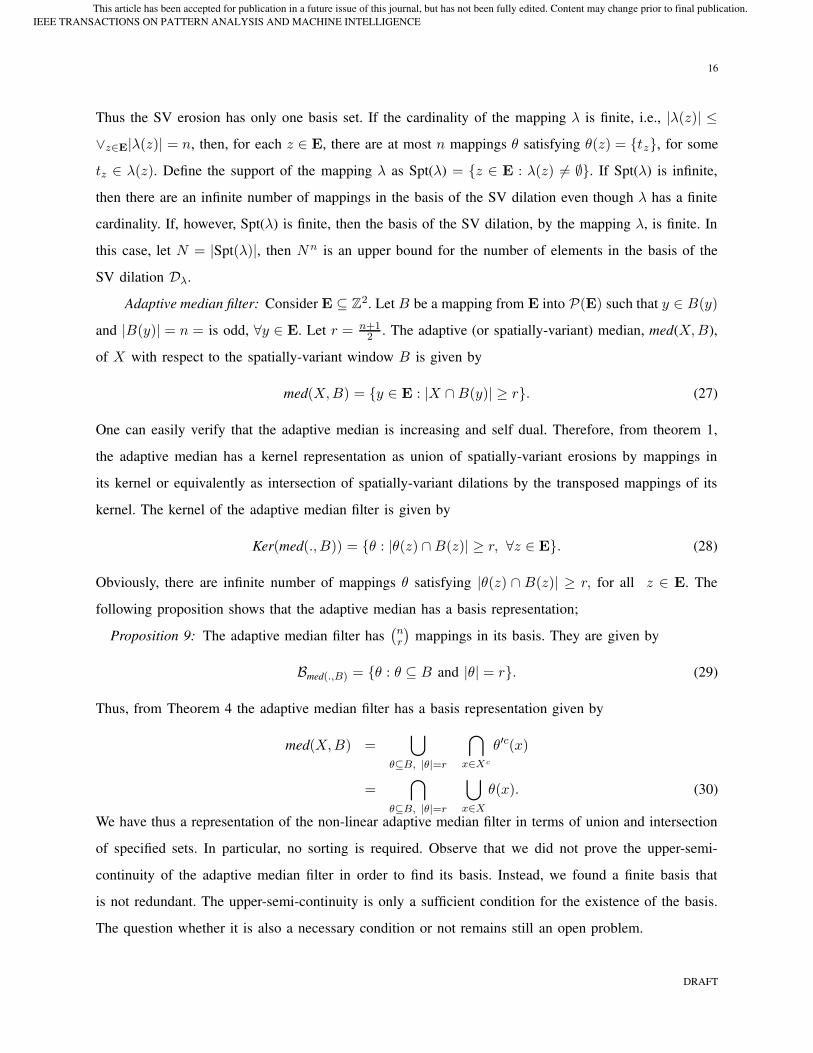
Adaptive median filter: Consider E ⊆ Z2. Let B be a mapping from E into P(E) such that y ∈ B(y)

and |B(y)| = n = is odd, ∀y ∈ E. Let r = n+12 . The adaptive (or spatially-variant) median, med(X,B),

of X with respect to the spatially-variant window B is given by

med(X,B) = {y ∈ E : |X ∩ B(y)| ≥ r}. (27)

One can easily verify that the adaptive median is increasing and self dual. Therefore, from theorem 1,

the adaptive median has a kernel representation as union of spatially-variant erosions by mappings in

its kernel or equivalently as intersection of spatially-variant dilations by the transposed mappings of its

kernel. The kernel of the adaptive median filter is given by

Ker(med(., B)) = {θ : |θ(z) ∩ B(z)| ≥ r, ∀z ∈ E}. (28)

Obviously, there are infinite number of mappings θ satisfying |θ(z) ∩ B(z)| ≥ r, for all z ∈ E. The

following proposition shows that the adaptive median has a basis representation;

Proposition 9: The adaptive median filter has(nr

)mappings in its basis. They are given by

Bmed(.,B) = {θ : θ ⊆ B and |θ| = r}. (29)

Thus, from Theorem 4 the adaptive median filter has a basis representation given by

med(X,B) =⋃

θ⊆B, |θ|=r

⋂x∈Xc

θ′c(x)

=⋂

θ⊆B, |θ|=r

⋃x∈X

θ(x). (30)

We have thus a representation of the non-linear adaptive median filter in terms of union and intersection

of specified sets. In particular, no sorting is required. Observe that we did not prove the upper-semi-

continuity of the adaptive median filter in order to find its basis. Instead, we found a finite basis that

is not redundant. The upper-semi-continuity is only a sufficient condition for the existence of the basis.

The question whether it is also a necessary condition or not remains still an open problem.

DRAFT


17

Spatially-Variant Hit-or-Miss transform: The spatially-variant hit-or-miss transform . ⊗ (θ1, θ2) is

given by

X ⊗ (θ1, θ2) = {z ∈ ξ : θ1(z) ⊆ X ⊆ θ2(z)} (X ∈ P(ξ)). (31)

Consider mappings θ1 and θ2 from E into P(E). Let us use [θ1, θ2] to denote the mapping segment

given by [θ1, θ2] = {θ : θ1 ⊆ θ ⊆ θ2}. In the following theorem we provide the spatially-variant

kernel representation of operators in O (not necessarily increasing) based on spatially-variant hit-or-miss

transforms.

Theorem 5: Given a mapping ψ ∈ O, we have

ψ(X) =⋃

[θ1,θ2]⊆Ker(ψ)

(X ⊗ (θ1, θ2)) (X ∈ P(ξ)). (32)

The representation in Theorem 5 is redundant. To see this, let [θ1, θ2] and [θ3, θ4] be two segments

such that [θ1, θ2] ⊆ [θ3, θ4], i.e., θ3 ≤ θ1 ≤ θ2 ≤ θ4. Then, X ⊗ [θ1, θ2] ⊆ X ⊗ [θ3, θ4], for every

X ∈ P(E). Therefore, in the representation of an operator by SV hit-or-miss transforms, if the above

segments [θ1, θ2] and [θ3, θ4] are contained in Ker(ψ), the mapping . ⊗ (θ1, θ2) will be redundant.

The basis of ψ, in this representation, is defined as the set of all the maximal intervals contained in

Ker(ψ). An interval is maximal if no other interval contained in Ker(ψ) properly contains it. Bannon and

Barrera [2] have a similar definition of the basis in the special case of translation-invariant operators.

The extension of the derivation of the existence of the minimal basis to the spatially-variant case can

be carried out based on the development in [2] and is out of the scope of this paper. One can verify

that under the same sufficient condition of upper-semi-continuity, an operator, the domain of which is

the collection of closed subsets of an Euclidean space, has a minimal kernel representation in terms of

spatially-variant hit-or-miss transforms.

VI. SIMULATIONS

The simulation results presented in this section are intended to illustrate the general theory of SV

mathematical morphology and show its power in image analysis applications. For more practical examples

of specific application-oriented spatially-variant structuring elements, we refer the reader to the references

cited in the introduction.

A. Spatially-Variant Opening by Reconstruction and Segmentation

Morphological filters by reconstruction [13], [55], [59], use an image, called a “marker” (usually a

filtered version of the original image) to reconstruct objects or features of interest in the original image

DRAFT


18

called the “mask”. Thus, filters by reconstruction can be used for segmentation. However, a deceptive

problem arises when dealing with noisy images: The reconstruction process reconnects portions of the

noise along with the useful information in the image. This problem is intolerable in some applications

such as contour extraction from noisy 2-D and 3-D medical images. We illustrate the morphological

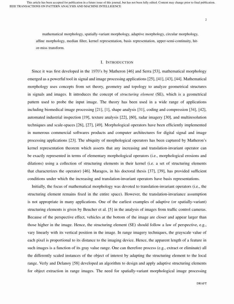
opening by reconstruction scheme in noisy environments using the binary image of blobs in Fig. 2(a)

and its corrupted version by a germ-grain noise model [53] in Fig. 2(b). In morphological opening by

reconstruction, the eroded image is used as the marker image. Then, the reconstruction process restores,

through iterative dilations, the blobs that have not been totally removed by the erosion. Figure 2(c) shows

the output of the translation-invariant opening by reconstruction using the rhombus SE. Since the erosion

by the rhombus SE is unable to eliminate the structures of noise bigger than the rhombus, most of the

noise is reconstructed along with the original blobs. So, in a second experiment, we eroded the noisy

image by the rhombus SE dilated 3 times to eliminate all the noise in the marker image. Nevertheless,

the reconstructed image is still noisy as shown in Fig. 2(d). The noise persists in the reconstructed image

because it is connected to the original blobs and hence is viewed by the reconstruction algorithm as

part of the blobs. A simple solution to avoid the noise reconstruction problem is to spatially-vary the

structuring element while eroding to form the marker image. The strategy adopted here is quite intuitive

and can be summarized as follows:

1) At each pixel z of the image, decide, by exploring its neighborhood, whether it belongs to a noise-

grain or not (the germ-grain noise model is assumed to be known, a priori). The detection of the

presence of a noise-grain C(z) centered at the pixel z is determined by selecting the largest possible

grain C which is present or absent in the degraded image Y (i.e., C +{z} ⊆ Y or C +{z} ⊆ Y c).

The SE mapping of the SV erosion is then selected as follows:

θ(z) =

⎧⎨⎩

C(z) ⊕ S, if z is detected as a noisy pixel;

S, otherwise,(33)

where S denotes the rhombus structuring element. This choice of the SE mapping ensures that all

noise-grains are removed completely (since the local SE is larger than the size of the noise-grain),

while preserving the small main blobs in the image (which have size bigger than the rhombus).

The marker image is then obtained by SV erosion of the noisy image or the mask.

2) Label the pixels in the mask image as follows: If a pixel was detected as noisy in step 1), label it

differently from the main blobs (even if it is connected to a main blob). Each main blob is assigned

a unique number.

3) Determine the labels which contain at least a pixel of the marker image.

DRAFT


19

4) the reconstructed image is obtained by removing all the pixels whose label is not one of the previous

ones.

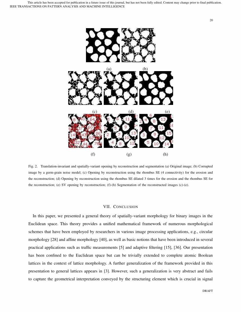
The result of SV opening by reconstruction is displayed in Fig. 2(e). The noise is not reconstructed with

the original blobs. This is important not only for denoising but also for segmentation. A persisting noise

in the reconstructed image has deleterious consequences for segmentation as it is either classified as main

blobs (see Fig. 2(f)) or merges originally disconnected blobs (see Fig. 2(g)) and, in both cases, results

in erroneous segmentation and blob detection. The third row of Fig. 2 displays the segmentation results.

For visual display, we labelled each segmented blob by a number. The opening by reconstruction using

the rhombus SE (resp. the rhombus SE dilated 3 times) detected 104 different blobs (resp. 15 blobs)

whereas the SV opening by reconstruction resulted in the correct segmentation of the original 18 blobs.

B. Spatially-Variant Morphological Skeleton Representation

The translation-invariant morphological skeleton representation [35], [53] is known to be redundant,

in the sense that a smaller subset of the morphological skeleton is sufficient for perfect reconstruction of

the original image [7], [33], [38]. It has been shown that efficient encoding of the skeleton representation

using run-length type codes can be used to provide an efficient compression routine for binary images

[34], [42]. For practical purposes, we can assume that the coding efficiency of the skeleton depends only

on the number of its points [42]. Therefore, minimizing the cardinality of the morphological skeleton

representation, under the constraint of exact reconstruction, is crucial for efficient compression of binary

images. In [7], we extended the morphological skeleton representation framework presented in [51] to the

spatially-variant case. The theoretical properties of the SV morphological skeleton representation and the

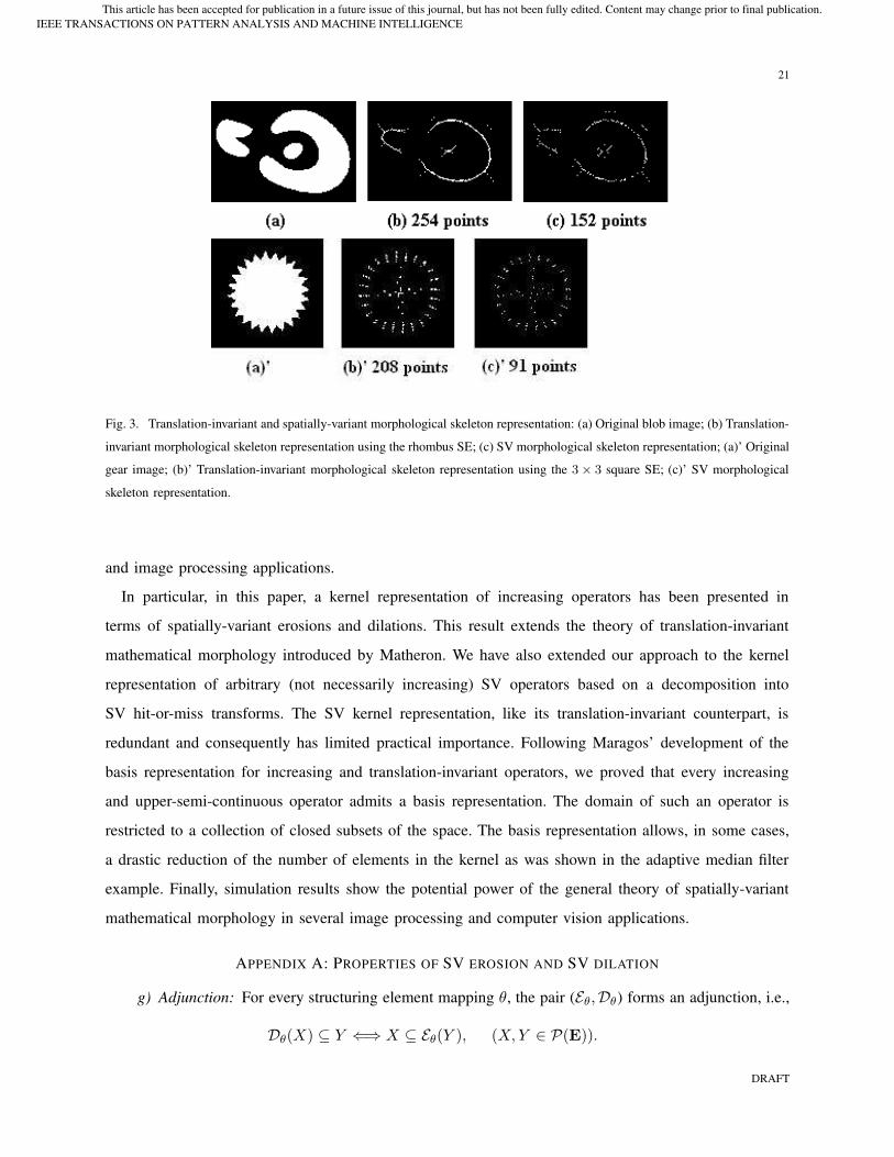
conditions for its invertibility were investigated in [7]. Figure 3 shows the results of SV morphological

skeleton representation compared to its translation-invariant counterpart for two binary images. The SV

morphological skeleton representation has a cardinality that is less than 60% of the cardinality of its

translation-invariant counterpart. Given an initial SE, B, the algorithm iteratively selects the center of

the dilated structuring element, nB = B ⊕B · · · ⊕B (n times), that maximally intersects the image, for

some integer n. The union of these center points forms the SV morphological skeleton representation.

The exact reconstruction of the original image is guaranteed given the SE B, the set of center points and

their corresponding integer n.

DRAFT


20

(a) (b)

(c) (d) (e)

(f) (g) (h)

Fig. 2. Translation-invariant and spatially-variant opening by reconstruction and segmentation (a) Original image; (b) Corrupted

image by a germ-grain noise model; (c) Opening by reconstruction using the rhombus SE (4 connectivity) for the erosion and

the reconstruction; (d) Opening by reconstruction using the rhombus SE dilated 3 times for the erosion and the rhombus SE for

the reconstruction; (e) SV opening by reconstruction; (f)-(h) Segmentation of the reconstructed images (c)-(e).

VII. CONCLUSION

In this paper, we presented a general theory of spatially-variant morphology for binary images in the

Euclidean space. This theory provides a unified mathematical framework of numerous morphological

schemes that have been employed by researchers in various image processing applications, e.g., circular

morphology [28] and affine morphology [40], as well as basic notions that have been introduced in several

practical applications such as traffic measurements [5] and adaptive filtering [15], [36]. Our presentation

has been confined to the Euclidean space but can be trivially extended to complete atomic Boolean

lattices in the context of lattice morphology. A further generalization of the framework provided in this

presentation to general lattices appears in [3]. However, such a generalization is very abstract and fails

to capture the geometrical interpretation conveyed by the structuring element which is crucial in signal

DRAFT


21

Fig. 3. Translation-invariant and spatially-variant morphological skeleton representation: (a) Original blob image; (b) Translation-

invariant morphological skeleton representation using the rhombus SE; (c) SV morphological skeleton representation; (a)’ Original

gear image; (b)’ Translation-invariant morphological skeleton representation using the 3 × 3 square SE; (c)’ SV morphological

skeleton representation.

and image processing applications.

In particular, in this paper, a kernel representation of increasing operators has been presented in

terms of spatially-variant erosions and dilations. This result extends the theory of translation-invariant

mathematical morphology introduced by Matheron. We have also extended our approach to the kernel

representation of arbitrary (not necessarily increasing) SV operators based on a decomposition into

SV hit-or-miss transforms. The SV kernel representation, like its translation-invariant counterpart, is

redundant and consequently has limited practical importance. Following Maragos’ development of the

basis representation for increasing and translation-invariant operators, we proved that every increasing

and upper-semi-continuous operator admits a basis representation. The domain of such an operator is

restricted to a collection of closed subsets of the space. The basis representation allows, in some cases,

a drastic reduction of the number of elements in the kernel as was shown in the adaptive median filter

example. Finally, simulation results show the potential power of the general theory of spatially-variant

mathematical morphology in several image processing and computer vision applications.

APPENDIX A: PROPERTIES OF SV EROSION AND SV DILATION

g) Adjunction: For every structuring element mapping θ, the pair (Eθ,Dθ) forms an adjunction, i.e.,

Dθ(X) ⊆ Y ⇐⇒ X ⊆ Eθ(Y ), (X,Y ∈ P(E)).

DRAFT


22

h) Duality: The SV erosion Eθ and SV dilation Dθ are dual operators, i.e.,

E∗θ (X) = Dθ′(X) (X ∈ P(E)).

i) Increasingness: For every structuring element mapping θ, the SV erosion Eθ and SV dilation Dθ

are increasing operators from P(E) to P(E).

j) Extensivity and anti-extensivity: If z ∈ θ(z), for all z ∈ E, then the SV erosion Eθ is anti-extensive

and the SV dilation Dθ is extensive, i.e.,

Eθ(X) ⊆ X, and X ⊆ Dθ(X) (X ∈ P(E)).

Observe that in the translation-invariant case with fixed structuring element B, i.e., θ(z) = B + z, the

condition z ∈ θ(z) reduces to 0 ∈ B.

k) Scaling with respect to the SE mapping: If θ1 ⊆ θ2, then

Eθ2(X) ⊆ Eθ1

(X), and Dθ1(X) ⊆ Dθ2

(X) (X ∈ P(E)).

l) Serial composition: Consider the mappings θ1 and θ2 from E into P(E). Let us use Eθ1(θ2) and

Dθ1(θ2) to denote the mappings from E into P(E) given by (Eθ1

(θ2))(z) = Eθ1(θ2(z)) and (Dθ1

(θ2))(z) =

Dθ1(θ2(z)), for every z ∈ E. Then, we have

Eθ2(Eθ1

) = EDθ1(θ2), and Dθ2

(Dθ1) = DDθ2

(θ′

1),

for every X ∈ P(E).

VIII. APPENDIX B: PROOF OF LEMMAS AND COROLLARIES

Proof: [Proof of Lemma 1] Let L be a linearly ordered subset of F . From [2, Lemma 4.1],⋂

L

is adherent to L. Since F is second countable, there exists a sequence {Xn}n∈N of elements of L

converging to⋂

L. The sequence {Xn}n∈N is itself a linearly ordered subset of L. Therefore, from [2,

Lemma 4.1],⋂

n∈NXn is adherent to the sequence {Xn}n∈N. The converging sequence {Xn}n∈N has a

unique adherent point and therefore⋂

L =⋂

n∈NXn. From the fact that the sequence {Xn}n∈N is itself

a linearly ordered subset of L, we conclude that Xn ↓⋂

L.

Proof: [Proof of Corollary 1] Consider an increasing operator ψ from G to G. Then, the dual mapping

ψ∗ is also increasing and maps F to F . Since ψ∗ is u.s.c., it admits a basis representation as union of

SV erosions (theorem 4). The result follows then easily by duality.

DRAFT


23

IX. APPENDIX C: PROOF OF PROPOSITIONS

Proof: [Proof of Proposition 1] Consider the mapping θX from E into P(E) given by

θX(z) =

⎧⎨⎩

X, z ∈ ψ(X);

E, z /∈ ψ(X),(34)

for some X ∈ P(E). Then, we have for any non-degenerate ψ ∈ O

ψ(θX(z)) =

⎧⎨⎩

ψ(X), z ∈ ψ(X);

E, z /∈ ψ(X).(35)

Therefore, we observe that z ∈ ψ(θX(z)), for every z ∈ E. So, from Definition 3, θX ∈ Ker(ψ).

Proof: [Proof of Proposition 2] Assume that ψ1(X) ⊆ ψ2(X) for every X ∈ P(E). From Definition

3, we observe that

θ ∈ ker (ψ1) =⇒ z ∈ ψ1(θ(z)),∀ z ∈ E

=⇒ z ∈ ψ2(θ(z)),∀ z ∈ E

=⇒ θ ∈ ker (ψ2).

Therefore, we notice that ker (ψ1) ⊆ ker (ψ2).

Assume now that ker (ψ1) ⊆ ker (ψ2). Let us consider the mapping θX from E into P(E) given by Eq.

(34) (with ψ −→ ψ1). From Eq. (35) we observe that z ∈ ψ1(θX(z)), for every z ∈ E. From Definition

3, we have

z ∈ ψ1(θX(z)),∀ z ∈ E =⇒ θX ∈ ker (ψ1)

=⇒ θX ∈ ker (ψ2)

=⇒ z ∈ ψ2(θX(z)),∀ z ∈ E.

Let us consider z ∈ ψ1(X). From Eq. (34) we observe that θX(z) = X. Therefore, z ∈ ψ2(θX(z)) =

ψ2(X). So, ψ1(X) ⊆ ψ2(X), for every X ∈ E. This completes the proof.

DRAFT


24

Proof: [Proof of Proposition 3]

(X c A) � z = {y : (A � y) ⊆ X} � z

= {y � z : (A � y) ⊆ X}

= {y : [A � (y �1

z)] ⊆ X}

= {y : [(A � y) �1

z] ⊆ X}

= {y : (A � y) ⊆ (X � z)}

= (X � z) c A.

Therefore, we proved equation (22). A similar argument can be used to prove equation (23).

Proof: [Proof of Proposition 4] Let ψ ∈ O be an increasing operator. Consider the mapping θX

defined in Eq. (34). θX ∈ Ker(ψ). Since ψ is increasing, we observe that every mapping θ from E into

P(E) such that θX ≤ θ is also in the kernel of ψ. This proves that Ker (ψ) is infinite.


a) Consider F ∈ F and let {xn}n∈N ⊂ Eθ(F ) be a sequence converging toward x ∈ E . By definition

of the SV erosion, we have θ(xn) ⊆ F , ∀n ∈ N. Since the mapping θ is continuous, θ(xn)F−→ θ(x). By

[46, Corollary 3(e)], we obtain θ(x) ⊆ F , which is equivalent to x ∈ Eθ(F ). Therefore, every convergent

sequence in Eθ(F ) has its limit point in Eθ(F ). Hence Eθ(F ) is closed.

b) Consider F ∈ F and let {xn}n∈N ⊂ Dθ(F ) be a sequence converging toward x ∈ E. By definition

of the SV dilation, we have θ′(xn) ∩ F �= ∅, ∀n ∈ N. So, for each n, there exists fn ∈ F such that

fn ∈ θ′(xn). Since θ′ is continuous and compact, we have θ′(xn)K−→ θ′(x). By [46, Theorem1-4-1],

there exists K0 ∈ K such that θ′(xn) ⊆ K0, ∀n and thus fn ∈ K0. By compactness of K0, there exists

a convergent subsequence fnk−→ f ∈ F (since F is closed). By condition 2 in [46, Theorem1-2-2],

fnk∈ F . Also, since fnk

is a convergent subsequence in θ′(xnk), f ∈ θ′(x). Hence, f ∈ θ′(x) ∩ F ,

which is equivalent to x ∈ Dθ(F ). Therefore, every convergent sequence in Dθ(F ) has its limit point in

Dθ(F ). Hence Dθ(F ) is closed.


a) Let {Fn}n∈N be a sequence in F converging toward F ∈ F . Let x ∈ lim Eθ(Fn). Then, by [46,

Proposition 1-2-3 (b)], there exists a subsequence xnp∈ Eθ(Fnp

) converging toward x. By definition

of the SV erosion, θ(xnp) ⊆ Fnp

. By continuity of the mapping θ, we have θ(xnp)

F−→ θ(x). Using

[46, Corollary 3(e)], we have θ(x) ⊆ F , which is equivalent to x ∈ Eθ(F ). Therefore, every point

x ∈ lim Eθ(Fn) belongs also to Eθ(F ). Hence lim(Eθ(Fn)) ⊆ Eθ(F ). By [46, Proposition 1-2-4 (a)], we

DRAFT


25

conclude that Eθ is upper-semi-continuous.

b) Let {Fn}n∈N be a sequence in F converging toward F ∈ F . Let x ∈ limDθ(Fn). Then, by [46,

Proposition 1-2-3(b)], there exists a subsequence xnp∈ Dθ(Fnp

) converging toward x. So, there exists

fnp∈ Fnp

such that fnp∈ θ′(xnp

). Since θ′ is continuous and compact, we have θ′(xnp)

K−→ θ′(x) and

by [46, Theorem 1-4-1], there exists K0 ∈ K such that K0 ⊃ θ′(xnp), ∀np. In particular, fnp

∈ K0.

By compactness of K0, the sequence {fnp} admits a convergent subsequence toward a point f ∈ F .

Without loss of generality, we can assume that the latter subsequence is fnp. By Criterion 2 of [46,

Theorem1-2-2], f ∈ θ′(x). Hence, we have f ∈ θ′(x)∩F , which is equivalent to x ∈ Dθ(F ). Therefore,

every point x ∈ limDθ(Fn) belongs also to Dθ(F ). Hence lim(Dθ(Fn)) ⊆ Dθ(F ). By [46, Proposition

1-2-4(a)], we conclude that Dθ is upper-semi-continuous.


a) Consider first the union of two increasing and upper-semi-continuous operators, ψ = ψ1 ∪ ψ2. We

have, for X,Y ∈ F such that X ⊆ Y , ψ(X) = ψ1(X) ∪ ψ2(X) ⊆ ψ1(Y ) ∪ ψ2(Y ) = ψ(Y ). Thus, ψ

is increasing. To prove the upper-semi-continuity of ψ, we use proposition 5. Consider, then, a sequence

{Xn}n∈N ∈ F such that Xn ↓ X. We have, for every n,Xn ⊇ Xn+1 ⊇ X. Therefore, since ψ is

increasing, ψ(Xn) ⊇ ψ(Xn+1) ⊇ ψ(X). Thus, the sequence {ψ(Xn)} is decreasing. In particular, we

have ψ(Xn) ⊇ ψ(X), for every n ∈ N. Thus

⋂n∈N

ψ(Xn) ⊇ ψ(X). (36)

Consider now x ∈⋂

n ψ(Xn). That is x ∈⋂

n(ψ1(Xn)∪ψ2(Xn)). So, x ∈ ψ1(Xn)∪ψ2(Xn), for every

n. We distinguish 2 cases:

case 1: x ∈ ψ1(Xn) (or ψ2(Xn)) only for a finite number of integers n. Since the problem is symmetric

in ψ1 and ψ2, we can assume, without loss of generality, that x ∈ ψ1(Xn) only for a finite number of

integers n. That is there exists an integer N0 such that for every n ≥ N0, x /∈ ψ1(Xn). Thus, we have

for every n ≥ N0, x ∈ ψ2(Xn). Therefore x ∈⋂

n≥N0ψ2(Xn) =

⋂n∈N

ψ2(Xn) = ψ2(X), where the

1st equality follows from the fact that ψ2 is increasing and the 2nd equality follows from the upper-semi-

continuity of ψ2. Thus, x ∈ ψ2(X) ∪ ψ1(X) = ψ(X).

case 2: x ∈ ψ1(Xn) and ψ2(Xn) for an infinite (and countable) number of integers n. That is, for every

N0, we have x ∈ ψ1(Xn) ∩ ψ2(Xn), for some n ≥ N0. Due to the monotonicity property of ψ1 and

ψ2, we also have that x ∈ ψ1(Xn) ∩ ψ2(Xn), for every n ≤ N0. Hence, x ∈ ψ1(Xn) ∩ ψ2(Xn), for

every n ∈ N. Thus, x ∈⋂

n(ψ1(Xn) ∩ ψ2(Xn)) = (⋂

n ψ1(Xn))⋂

(⋂

n ψ2(Xn)) = ψ1(X) ∩ ψ2(X). In

DRAFT


26

particular, x ∈ ψ1(X) ∪ ψ2(X) = ψ(X). Finally, we have

ψ(X) ⊇⋂n∈N

ψ(Xn). (37)

Equations (36) and (37) and the increasing property of ψ are equivalent to ψ(Xn) ↓ ψ(X). Therefore,

ψ is upper-semi-continuous.

b) Consider now the intersection of two increasing and upper-semi-continuous operators, ψ ′ = ψ1∩ψ2.

We have, for X,Y ∈ F such that X ⊆ Y , ψ′(X) = ψ1(X) ∩ ψ2(X) ⊆ ψ1(Y ) ∩ ψ2(Y ) = ψ′(Y ). Thus,

ψ′ is increasing. Consider now a sequence {Xn}n∈N ∈ F such that Xn ↓ X. Since ψ′ is increasing, the

sequence {ψ′(Xn)}n∈N is decreasing. We have

x ∈⋂n

ψ′(Xn) ⇐⇒ x ∈⋂n

(ψ1(Xn) ∩ ψ2(Xn))

⇐⇒ x ∈ (⋂n

ψ1(Xn)) ∩ (⋂n

ψ2(Xn))

⇐⇒ x ∈ ψ1(X) ∩ ψ2(X) ⇐⇒ x ∈ ψ′(X).

So, ψ′(Xn) ↓ ψ′(X). Therefore, ψ′ is upper-semi-continuous.

Proof: [Proof of Proposition 9] Let A be the set of the(nr

)subsets of B containing exactly r points.

We denote by ker the kernel of the adaptive median filter. For every θ ∈ Ker, there exists λ ∈ A such

that λ ≤ θ. So, by property k) in Appendix A, Eθ ⊆ Eλ. Thus⋃

θ∈Ker Eθ ⊆⋃

λ∈A Eλ. Conversely, we

have A ⊆ Ker. So,⋃

λ∈A Eλ ⊆⋃

θ∈Ker Eθ. Therefore,⋃

λ∈A Eλ =⋃

θ∈Ker Eθ. We claim that the basis of

the kernel of the adaptive median filter is A. Otherwise, there exists θ ∈ Ker such that θ < λ, for every

λ ∈ A. In particular, |θ| < r. This contradicts the fact that θ ∈ ker and establishes A as the basis of the

adaptive median operator.

APPENDIX D: PROOF OF THEOREMS

Proof: [Proof of Theorem 1] Assume that ψ(X) =⋃

θ∈Ker(ψ) Eθ(X), for every X ∈ P(E). ψ is then

increasing as union of increasing operators. Assume now that ψ is increasing and consider X ∈ P(E).

Let z ∈ ψ(X). Let us also consider the mapping θX from E into P(E) given by Eq. (34). θX ∈ ker(ψ).

So, θX(z) = X. Hence, by definition of the SV erosion, z ∈ EθX(X) ⊆

⋃θ∈Ker(ψ) Eθ(X). Therefore,

ψ(X) ⊆⋃

θ∈Ker(ψ)

Eθ(X). (38)

Let us now consider z ∈⋃

θ∈Ker(ψ) Eθ(X). So, there exists θ ∈ Ker(ψ) such that z ∈ Eθ(X). From the

definition of the SV erosion, this is equivalent to the existence of θ ∈ Ker(ψ) such that θ(z) ⊆ X. Since,

DRAFT


27

θ ∈ Ker(ψ) and ψ is increasing, we observe that z ∈ ψ(θ(z)) ⊆ ψ(X). Finally, we have shown that

⋃θ∈Ker(ψ)

Eθ(X) ⊆ ψ(X). (39)

From Eqs. (38) and (39), we obtain the desired kernel representation of the increasing operator ψ. Since

the class of increasing operators is closed under duality, the representation of an increasing operator as

an intersection of SV dilations by the transposed mappings in the kernel of its dual is easily obtained by

duality from its representation as union of SV erosions by mappings in the kernel.

Proof: [Proof of Theorem 2] Let ψ ∈ O′

be an increasing and u.s.c. operator. From proposition 4,

the kernel of ψ is a non-empty partially ordered set. Consider a linearly ordered subset L of Ker (ψ).

For every z ∈ E,Lz = {θ(z) : θ ∈ L} is a linearly ordered subset of F . From Lemma 1, there exists

a sequence {θn(z) : n ∈ N, θn ∈ L} such that θn(z) ↓⋂

n∈Nθn(z) =

⋂Lz. From the fact that ψ is an

increasing u.s.c. operator, we have

ψ(θn(z)) ↓ ψ(⋂

Lz) (z ∈ E). (40)

By the uniqueness of limit points in Hausdorff spaces, we obtain

ψ(⋂

Lz) =⋂n∈N

ψ(θn(z)) (z ∈ E). (41)

From the above equation and using the fact that θn ∈ Ker(ψ), ∀n ∈ N, we observe that the operator

from E into F defined by

(∧L)(z) =⋂

Lz (z ∈ E), (42)

is an element of Ker (ψ), where ∧L is the infimum of the linearly ordered subset L. Finally, we have

showed that every linearly ordered subset of Ker (ψ) has an infimum in Ker (ψ). Using Zorn’s Lemma

[32], we conclude that the kernel of ψ has a minimal element.


be an increasing u.s.c. operator and let θA ∈ Ker(ψ).

Then, there exists θB ∈ Ker(ψ) such that θB ≤ θA, otherwise θA is a minimal element. Therefore, for

every θA ∈ Ker(ψ), we can construct a decreasing family L of Ker(ψ) containing θA. From the fact that

L is a linearly ordered subset of Ker(ψ) and from Hausdorff’s Maximality Principle [37], there exists a

maximal linearly ordered subset M of Ker(ψ) containing L. Let θM (z) = (∧M)(z) =⋂

θ∈M θ(z), for

every z ∈ E. From the proof of Theorem 2, θM ∈ Ker(ψ). We have θM ≤⋂

L ≤ θA. Therefore, θM

is a minimal element of Ker(ψ) for otherwise, there exists θY ∈ Ker(ψ) such that θY ≤ θM ; the subset

M∪{θY } is then a linearly ordered subset of Ker(ψ) containing M; this contradicts the maximality of

M. Finally we have shown that θM is a minimal element and θM ≤ θA. This completes the proof.

DRAFT


28


be an increasing and u.s.c. operator. From the fact that

Bψ ⊆ Ker(ψ), we have⋃

θM∈BψEθM

(X) ⊆⋃

θ∈Ker(ψ) Eθ(X), for every X ∈ F . From Theorem 3,

every θ ∈ Ker(ψ) contains a minimal element θM ∈ Bψ . Therefore, Eθ ⊆ EθM. So,

⋃θ∈Ker(ψ) Eθ(X) ⊆

⋃θM∈Bψ

EθM(X), for every X ∈ F . The result then follows by antisymmetry of the partial order ⊆.

Proof: [Proof of Theorem 5] Let ψ ∈ O. We know that any subset S of a partially ordered set P

can be properly covered by the union of the closed intervals of P contained in S (see [2, Lemma 2.1]

for a proof). Since Ker(ψ) is a partially-ordered set and the mapping segment [θ1, θ2] is a closed interval,

we have

Ker(ψ) =⋃

{[θ1, θ2] : [θ1, θ2] ⊆ Ker(ψ)}. (43)

On the other hand, we observe that

Ker(. ⊗ (θ1, θ2)) = [θ1, θ2]. (44)

Combining Eqs. (43) and (44), we obtain

Ker(ψ) =⋃

{Ker(. ⊗ (θ1, θ2)) : [θ1, θ2] ⊆ Ker(ψ)}. (45)

From Proposition 2, the mapping ψ �→ Ker(ψ) is an isomorphism. So, by applying the corresponding

inverse mapping to both sides of Eq. (45), we obtain the desired result.

REFERENCES

[1] J. Angulo and J. Serra, “Automatic analysis of DNA microarray images using mathematical morphology,” Bioinformatics,

vol. 19, no. 5, pp. 553–562, 2003.

[2] G. J. F. Banon and J. Barrera, “Minimal representation for translation-invariant set mappings by mathematical morphology,”

SIAM Journal on Applied Mathematics, vol. 51, pp. 1782–1798, Deceber 1991.

[3] ——, “Decomposition of mappings between complete lattices by mathematical morphology - part I: General lattices,”

Signal Processing, vol. 30, no. 3, pp. 299–327, February 1993.

[4] R. G. Bartle, The Elements of Real Analysis. New York: J. Wiley & Sons, Inc., 1976.

[5] S. Beucher, J. M. Blosseville, and F. Lenoir, “Traffic spatial measurements using video image processing,” in Proceedings

of SPIE in Intelligent Robots and Computer Vision, vol. 848, November 1987, pp. 648–655.

[6] G. Birkhoff, Lattice theory. Providence, Rhode Island: American Mathematical Society, 1984.

[7] N. Bouaynaya, M. Charif-Chefchaouni, and D. Schonfeld, “Spatially-variant morphological restoration and skeleton

representation,” IEEE Transactions on Image Processing, vol. 15, no. 11, pp. 3579–3591, November 2006.

[8] M. Charif-Chefchaouni, “Morphological representation of non-linear operators: Theory and applications,” Ph.D. dissertation,

University of Illinois at Chicago, 1993.

[9] M. Charif-Chefchaouni and D. Schonfeld, “Spatially-variant mathematical morphology,” in Proceedings of the IEEE

International Conference on Image Processing (ICIP), vol. 2, November 1994, pp. 555–559.

DRAFT


29

[10] C.-S. Chen, J.-L. Wu, and Y.-P. Hung, “Statistical analysis of space-varying morphological openings with flat structuring

elements,” IEEE Transactions On Signal Processing, vol. 44, no. 4, pp. 1010–1014, April 1996.

[11] ——, “Theoretical aspects of vertically invariant gray-level morphological operators and their application on adaptive signal

and image filtering,” IEEE Transactions On Signal Processing, vol. 47, no. 4, pp. 1049–1060, April 1999.

[12] F. Cheng and A. N. Venetsanopoulos, “An adaptive morphological filter for image processing,” IEEE Transactions on

Image Processing, vol. 1, no. 4, pp. 533–539, October 1992.

[13] J. Crespo, J. Serra, and R. W. Schafer, “Theoretical aspects of morphological filters by reconstruction,” Signal Processing,

vol. 47, no. 2, pp. 201–225, November 1995.

[14] O. Cuisenaire, “Locally adaptable mathematical morphology,” in IEEE International Conference on Image Processing

(ICIP), vol. 2, September 2005, pp. 125–128.

[15] J. Debayle and J. C. Pinoli, “General adaptive neighborhood image processing - part I: Introduction and theoretical aspects,”

Journal of Mathematical Imaging and Vision, vol. 25, no. 2, pp. 245–266, September 2006.

[16] ——, “General adaptive neighborhood image processing - part II: Practical application examples,” Journal of Mathematical

Imaging and Vision, vol. 25, no. 2, pp. 267–284, September 2006.

[17] E. R. Dougherty and C. R. Giardina, “A digital version of the matheron representation theorem for increasing τ -mappings

in terms of a basis for the kernel,” in IEEE Computer Vision and Pattern Recognition, Miami, June 1986, pp. 534–536.

[18] ——, Morphological Methods in Image Processing. Englewood Cliffs: Prentice-Hall, Inc., 1988.

[19] T. Fang, M. A. Jafari, S. C. Danforth, and A. Safari, “Signature analysis and defect detection in layered manufacturing of

ceramic sensors and actuators,” Machine Vision and Applications, vol. 15, no. 2, pp. 63–75, December 2003.

[20] R. Gordon and R. M. Rangayyan, “Feature enhancement of mammograms using fixed and adaptive neighborhoods,” Applied

Optics, vol. 23, no. 4, pp. 560–64, February 1984.

[21] J. Goutsias and S. Batman, “Morphological methods for biomedical image analysis,” in Handbook of Medical Imaging,

Progress in Medical Image Processing and Analysis, M. Sonka and J. M. Fitzpatrick, Eds., vol. 3. SPIE Optical Engineering

Press, 2000, pp. 175–272.

[22] A. G. Hanbury and J. Serra, “Analysis of oriented textures using mathematical morphology,” in Vision with Non-Traditional

Sensors, Austria, September 2002.

[23] J. C. Handley, “Minimal-memory bit-vector architecture for computational mathematical morphology using subspace

projections,” IEEE Transactions on Image Processing, vol. 14, no. 8, pp. 1088–1095, August 2005.

[24] H. J. A. M. Heijmans, “Mathematical morphology: an algebraic approach,” CWI Newsletter, vol. 14, pp. 7 – 27, 1987.

[25] ——, Morphological image operators. Boston: Academic Press, 1994.

[26] H. J. A. M. Heijmans and J. Goutsias, “Nonlinear multiresolution signal decomposition schemes -I: Morphological

pyramids,” IEEE Transactions on Image Processing, vol. 9, no. 11, pp. 1862–1876, November 2000.

[27] ——, “Nonlinear multiresolution signal decomposition schemes -II: Morphological wavelets,” IEEE Transactions on Image

Processing, vol. 9, no. 11, pp. 1897–1913, November 2000.

[28] H. J. A. M. Heijmans and C. Ronse, “The algebraic basis of mathematical morphology - I: Dilations and erosions,”

Computer Vision, Graphics and Image Processing: Image Understanding, vol. 50, no. 3, pp. 245–295, June 1990.

[29] ——, “The algebraic basis of mathematical morphology - II: Openings and closings,” Computer Vision, Graphics and

Image Processing: Image Understanding, vol. 54, no. 1, pp. 74–97, July 1991.

[30] S. Hou, S. Wu, and S. Ma, “Doppler frequency extraction of radar echo signal based on time-frequency analysis and

DRAFT


30

morphological operation,” in Proceedings of the International Conference on Signal Processing (ICSP), vol. 3, 2004, pp.

2017–2020.

[31] A. C. Jalba, M. H. F. Wilkinson, and J. B. T. M. Roerdink, “Shape representation and recognition through morphological

curvature scale spaces,” IEEE Transactions on Image Processing, vol. 15, no. 2, pp. 331–341, February 2006.

[32] A. N. Kolmogoroff and S. V. Fomin, Introductory Real Analysis. New York: Dover, 1975.

[33] R. Kresch and D. Malah, “Morphological reduction of skeleton redundancy,” Signal Processing, vol. 38, no. 1, pp. 143–151,

July 1994.

[34] ——, “Skeleton-based morphological coding of binary images,” IEEE Transactions on Image Processing, vol. 7, no. 10,

pp. 1387–1399, October 1998.

[35] C. Lantuejoul, “La squelettization et son application aux mesures topologuiques des mosaiques polycristallines,” Ph.D.

dissertation, School of Mines, Paris, France, 1978.

[36] R. Lerallut, M. Goehm, E. Decenciere, and F. Meyer, “Noise reduction in 3D images using morphological amoebas,” in

IEEE International Conference on Image Processing (ICIP), vol. 1, September 2005, pp. 109–112.

[37] P. A. Maragos, “A unified theory of translation-invariant systems with applications to morphological analysis and coding

of images,” Ph.D. dissertation, Georgia Institute of Technology, July 1985.

[38] ——, “Pattern spectrum and multiscale shape representation,” IEEE Transactions on Pattern Analysis and Machine

Intelligence, vol. 11, pp. 701–716, July 1989.

[39] ——, “A representation theory for morphological image and signal processing,” IEEE Transactions on Pattern Analysis

and Machine Intelligence, vol. 11, no. 6, pp. 586–599, June 1989.

[40] ——, “Affine morphology and affine signal models,” in Proceedings of SPIE in Image Algebra and Morphological Image

Processing, vol. 1350, 1990, pp. 31–43.

[41] ——, Morphological Filtering For Image Enhancement And Feature Detection. Elsevier Academic Press, 2005, ch. 3,

pp. 135–156.

[42] P. A. Maragos and R. W. Schafer, “Morphological skeleton representation and coding of binary images,” IEEE Transactions

on Acoustics, Speech, and Signal Processing, vol. 34, no. 5, pp. 1228–1244, October 1986.

[43] ——, “Morphological filters - part I: Their set-theoric analysis and relations to linear shift-invariant filters,” IEEE

Transactions on Acoustics, Speech, and Signal Processing, vol. 35, no. 8, pp. 1153–1169, August 1987.

[44] ——, “Morphological filters - part II: Their relation to median, order-statistics and stack filters,” IEEE Transactions on

Acoustics, Speech, and Signal Processing, vol. 35, 1987.

[45] I. Masayasu, T. Masayoshi, and N. Akira, “Morphological operations by locally variable structuring elements and their

applications to region extraction in ultrasound images,” Systems and Computers in Japan, vol. 34, no. 3, pp. 33–43,

February 2003.

[46] G. Matheron, Random Sets and Integral Geometry. New York: J Wiley & Sons, 1975.

[47] Morales, “Adaptive structuring element for noise and artifact removal,” in Proceedings of the Conference on Information

Sciences and Systems, March 1989.

[48] J. B. T. M. Roerdink, “Group morphology,” Pattern Recognition, vol. 33, no. 6, pp. 877–895, 2000.

[49] ——, “Multiresolution maximum intensity volume rendering by morphological adjunction pyramids,” IEEE Transactions

on Image Processing, vol. 12, no. 6, pp. 653–660, June 2003.

[50] J. B. T. M. Roerdink and H. J. A. M. Heijmans, “Mathematical morphology for structuring elements without translation

symmetry,” Signal Processing, vol. 15, no. 3, pp. 271–277, 1988.

DRAFT


31

[51] D. Schonfeld and J. Goutsias, “Morphological representation of discrete and binary images,” IEEE Transactions on Signal

Processing, vol. 39, no. 6, pp. 1369–1379, June 1991.

[52] ——, “Optimal morphological pattern restoration from noisy binary images,” IEEE Transactions on Pattern Analysis and

Machine Intelligence, vol. 13, no. 1, pp. 14–29, January 1991.

[53] J. Serra, Image Analysis and Mathematical Morphology. San Diego, Ca.: Academic Press, 1982.

[54] ——, Image Analysis and Mathematical Morphology Theoretical Advances. New York: Academic Press, 1988, vol. 2.

[55] J. Serra and P. Salembier, “Connected operators and pyramids,” in Proceedings of SPIE, vol. 2030, 1993, pp. 65–76.

[56] F. Y. Shih and S. Cheng, “Adaptive mathematical morphology for edge linking,” International Journal on Information

SciencesłInformatics and Computer Science, vol. 167, pp. 9–21, December 2004.

[57] K. Shoji, “Generalized skeleton representation and adaptive rectangular decomposition of binary images,” in Proceedings

of SPIE in Image Algebra and Morphological Image Processing, J. C. Serra, Ed., vol. 1769, June 1992, pp. 404–415.

[58] J. G. Verly and R. L. Delanoy, “Adaptive mathematical morphology for range imagery,” IEEE Transactions on Image

Processing, vol. 2, no. 2, pp. 272–275, April 1993.

[59] L. Vincent, “Morphological grayscale reconstruction in image analysis:applications and efficient algorithms,” IEEE

Transactions on Image Processing, vol. 2, no. 2, pp. 176–201, April 1993.

[60] Y. Xia, D. Feng, and R. Zhao, “Morphology-based multifractal estimation for texture segmentation,” IEEE Transactions

on Image Processing, vol. 15, no. 3, pp. 614–623, March 2006.

[61] J. Xu, “A generalized discrete morphological skeleton transform with multiple structuring elements for the extraction of

structural shape components,” IEEE Transactions on Image Processing, vol. 12, no. 2, pp. 1677–1686, December 2003.

Nidhal Bouaynaya received the B.S. degree in Electrical and Computer Engineering from the Ecole

Nationale Superieure de l’Electronique et de ses Applications (ENSEA), France, in 2002, the M.S. degree

in Electrical and Computer Engineering from the Illinois Institute of Technology, Chicago, IL, in 2002, the

Diplome d’Etudes Approfondies in signal and image processing from ENSEA, France, in 2003, the M.S.

degree in Mathematics and the Ph.D. degree in Electrical and Computer Engineering from the University

of Illinois at Chicago, Chicago, IL, in 2007.

In fall 2007, she joined the University of Arkansas at Little Rock where she is currently an Assistant Professor in the

Department of Systems Engineering. Her research interests are in signal, image and video processing; mathematical morphology

and genomic signal processing.

Dr. Bouaynaya won the Best Student Paper Award in Visual Communication and Image Processing 2006.

DRAFT


32

Mohammed Charif-Chefchaouni received the B.S. and M.S. degrees in electrical engineering and

computer science from the Ecole Nationale Suprieure de l’Aronautique et de l’Espace, Toulouse, France,

in 1978 and 1980, respectively.

From 1980 to 1990 he was a lecturer of applied mathematrics and control at the Institut des Postes et

Tlcommunications, Rabat, Morocco. He received the Ph.D. degree in electrical and computer engineering

from the University of Illinois at Chicago, Chicago, IL, in 1993. He is currently the director of the Institut

National des Postes et Tlcommunications, Rabat, Morocco. His research interests are image modeling and analysis.

Dan Schonfeld was born in Westchester, Pennsylvania, on June 11, 1964. He received the B.S. degree in

Electrical Engineering and Computer Science from the University of California at Berkeley, and the M.S.

and Ph.D. degrees in Electrical and Computer Engineering from the Johns Hopkins University, in 1986,

1988, and 1990, respectively.

In 1990, he joined the University of Illinois at Chicago, where he is currently a Professor in the

Department of Electrical and Computer Engineering. Dr. Schonfeld has authored over 100 technical

papers in various journals and conferences. His current research interests are in signal, image, and video processing; video

communications, retrieval, and networks; image analysis and computer vision; and genomic signal processing.

Dr. Schonfeld was co-author of papers that won the Best Student Paper Awards in Visual Communication and Image Processing

2006 and IEEE International Conference on Image Processing 2006. He is currently serving as associate editor of the IEEE

Transactions on Image Processing on Image and Video Storage, Retrieval and Analysis and associate editor of the IEEE

Transactions on Circuits and Systems for Video Technology on Video Analysis. He has served as an associate editor of the

IEEE Transactions on Signal Processing on Multidimensional Signal Processing and Multimedia Signal Processing as well as

an associate editor of the IEEE Transactions on Image Processing on Nonlinear Filtering.

DRAFT


Documents

Theoretical Foundations of Spatially-Variant Mathematical ...nbouayna/PAMI1.pdf · Theoretical Foundations of Spatially-Variant Mathematical Morphology Part I: Binary Images Nidhal