IAEA-TECDOC-1520

Theoretical and ExperimentalStudies of Heavy Liquid Metal

Thermal HydraulicsProceedings of a technical meeting

held in Karlsruhe, Germany, 28–31 October 2003

October 2006

IAEA-TECDOC-1520

Theoretical and ExperimentalStudies of Heavy Liquid Metal

Thermal HydraulicsProceedings of a technical meeting

held in Karlsruhe, Germany, 28–31 October 2003

October 2006

The originating Section of this publication in the IAEA was:

Radiation and Transport Safety Section International Atomic Energy Agency

Wagramer Strasse 5 P.O. Box 100

A-1400 Vienna, Austria

THEORETICAL AND EXPERIMENTAL STUDIES OF HEAVY LIQUID METAL THERMAL HYDRAULICS

IAEA, VIENNA, 2006 IAEA-TECDOC-1520 ISBN 92–0–111806–6

ISSN 1011–4289 © IAEA, 2006

Printed by the IAEA in Austria October 2006

FOREWORD

Through the Nuclear Energy Department’s Technical Working Group on Fast Reactors (TWG-FR), the IAEA provides a forum for exchange of information on national programmes, collaborative assessments, knowledge preservation, and cooperative research in areas agreed by the Member States with fast reactor and partitioning and transmutation development programmes (e.g. accelerator driven systems (ADS)). Trends in advanced fast reactor and ADS designs and technology development are periodically summarized in status reports, symposia, and seminar proceedings prepared by the IAEA to provide all interested IAEA Member States with balanced and objective information.

The use of heavy liquid metals (HLM) is rapidly diffusing in different research and industrial fields. The detailed knowledge of the basic thermal hydraulics phenomena associated with their use is a necessary step for the development of the numerical codes to be used in the engineering design of HLM components. This is particularly true in the case of lead or lead-bismuth eutectic alloy cooled fast reactors, high power particle beam targets and in the case of the cooling of accelerator driven sub-critical cores where the use of computational fluid dynamic (CFD) design codes is mandatory.

Periodic information exchange within the frame of the TWG-FR has lead to the conclusion that the experience in HLM thermal fluid dynamics with regard to both the theoretical/numerical and experimental fields was limited and somehow dispersed. This is the case, e.g. when considering turbulent exchange phenomena, free-surface problems, and two-phase flows. Consequently, Member States representatives participating in the 35th Annual Meeting of the TWG-FR (Karlsruhe, Germany, 22–26 April 2002) recommended holding a technical meeting (TM) on Theoretical and Experimental Studies of Heavy Liquid Metal Thermal Hydraulics.

Following this recommendation, the IAEA has convened the Technical Meeting on Theoretical and Experimental Studies of Heavy Liquid Metal Thermal Hydraulics (28–31 October 2003). The TM was hosted by the Forschungszentrum Karlsruhe, Germany.

The scope of the TM was to provide a global forum for information exchange on the most recent theoretical and experimental studies of HLM thermal hydraulics.

The main objective of the TM was to assess the shortcomings of the present CFD codes used for HLM simulation and to identify future research needs, in both the numerical and experimental area.

The IAEA would like to express its appreciation to all the participants, authors of papers, chairpersons, and to the hosts at Forschungszentrum Karlsruhe.

The IAEA officer responsible for this publication was A. Stanculescu of the Division of Nuclear Power.

EDITORIAL NOTE

The papers in these proceedings are reproduced as submitted by the authors and have not undergone rigorous editorial review by the IAEA.

The views expressed do not necessarily reflect those of the IAEA, the governments of the nominating Member States or the nominating organizations.

The use of particular designations of countries or territories does not imply any judgement by the publisher, the IAEA, as to the legal status of such countries or territories, of their authorities and institutions or of the delimitation of their boundaries.

The mention of names of specific companies or products (whether or not indicated as registered) does not imply any intention to infringe proprietary rights, nor should it be construed as an endorsement or recommendation on the part of the IAEA.

The authors are responsible for having obtained the necessary permission for the IAEA to reproduce, translate or use material from sources already protected by copyrights.

CONTENTS

SUMMARY ............................................................................................................................... 1

SESSION 1: REVIEW OF THE STATE OF ART OF PRESENT CDF CODES

Turbulence modeling issues in ADS thermal and hydraulic analyses ....................................... 9 G. Groetzbach

Two CFD applications to the design of the active zone of HLM spallation targets................................................................................................................... 33 P. Roubin

CFD analysis of the thermal-hydraulic performance of the ESS target ................................... 49 E.M.J. Komen, F. Roelofs, J. Wolters, G. Hansen

Validation of CFD models with respect to the thermal-hydraulic design of the ESS target................................................................................................................... 59 J. Wolters, G. Hansen, E.M.J. Komen, F. Roelofs

CFD analysis of the heavy liquid metal flow field in the MYRRHA pool.............................. 77 E.M.J. Komen, P. Kupschus, K. Van Tichelen, H. Aït Abderrahim, F. Roelofs

Comparative analysis of the benchmark activity results on the ADS target model.......................................................................................................................... 89 A. Sorokin, G. Bogoslovskaia, V. Mikhin, S. Marzinuk

Free surface fluid dynamics code adaptation by experimental evidence for the MYRRHA spallation target .................................................................................... 101 K. Van Tichelen, P. Kupschus, M. Dierckx, H. Aït Abderrahim, F. Roelofs

Thermohydraulic behaviour in an ADS target model ............................................................ 111 A. Peña, G.A. Esteban, J. Sancho

Development and application of CFD codes MASKA-LM and PORT 3D for investigation of thermal hydraulics of lead cooled fast reactor BREST ............................ 119 A.A. Veremeev, V.Ya. Kumayev, A.A. Lebezov

CFD simulation of X-ADS downcomer thermal stratification .............................................. 135 V. Anissimov, A. Alemberti

Experiences from using the STAR-CD code for Pb-Bi-coolant flows .................................. 151 J. Carlsson, H. Wider

CFD simulation of SINQ HETSS mercury experiments ....................................................... 165 T.V. Dury

SESSION 2: REVIEW OF CURRENT AND PLANNED EXPERIMENTAL

HLM PROGRAMS Thermal hydraulic research and development needs for lead fast reactors............................ 195

J.J. Sienicki, D.C. Wade, C.P. Tzanos Thermohydraulic research for the core of the BREST reactor............................................... 213

A.V. Zhukov, A.D. Efanov, A.P. Sorokin, J.A. Kuzina, V.P. Smirnov, A.I. Filin, A.G. Sila-Novitsky, V.N. Leonov

Pre-test analysis of the MEGAPIE integral test with RELAP5 ............................................. 227 W.H. Leung, B. Sigg

Experimental determination of the local heat transfer coefficient for MEGAPIE target window using infrared thermography ................................................... 243 J.A. Patorski, F. Gröschel, I. Platnieks

Thermal-hydraulic ADS lead bismuth loop (tall) and experiments on a heat exchanger ............................................................................................................ 259 B.R. Sehgal, W.M. Ma, A. Karbojian

HELIOS for thermal-hydraulic behaviour of Pb-Bi cooled fast reactor peacer..................... 271 I.S. Lee, K.Y. Suh

Void-fraction measurements in two-phase nitrogen-mercury flows...................................... 295 P. Satyamurthy, N.S. Dixit, P. Munshi

SESSION 3: ELABORATION OF FUTURE ACTIVITIES

Studies on heavy liquid metal thermal-hydraulics: Existing test facilities and test programs............................................................................ 307 J.U. Knebel, C. Fazio

LIST OF PARTICIPANTS .................................................................................................... 315

SUMMARY

1. INTRODUCTION

The use of heavy liquid metals (HLM) is rapidly diffusing in different research and industrial fields. The detailed knowledge of the basic thermal hydraulics phenomena associated with their use is a necessary step for the development of the numerical codes to be used in the R&D as well as in the engineering design of HLM components. This is particularly true in the case of high power particle beam targets and in the case of the cooling of accelerator driven sub-critical cores where the use of computational fluid dynamic (CFD) design codes is mandatory.

The scope of the topical Technical Meeting on Theoretical and Experimental Studies of Heavy Liquid Metal Thermal Hydraulics was to provide a global forum for information exchange on the most recent theoretical and experimental studies of HLM thermal hydraulics. The main objective of the technical meeting was the assessment of the shortcomings of the present CFD codes used for HLM simulation and to propose future research activities, in both the numerical and experimental area.

More specifically, the technical meeting:

(i) Reviewed the state of the art of present CFD codes by: — Assessing their degree of precision and accuracy; — Identifying open issues in current turbulence models; — Identifying open issues in free surface phenomena and two-phase flows; — Addressing development needs of adequate physical models for HLM flows; — Addressing code validation issues.

(ii) Reviewed the current and planned experimental HLM programmes: — Description of capabilities of existing and planned HLM facilities and work

programme; — Instrumentation and measurement techniques; — Description of existing and planned benchmark experiments and databases; — Thermal hydraulics applications to ongoing projects on spallation targets and

accelerator driven systems (ADS); — Prospects for international collaboration and coordination of the experimental

activities.

(iii) Elaborated the needs for future activities: — Definition of numerical and experimental benchmarks (including required

databases); — International collaboration (networking and coordination among institutions

involved in HLM thermal hydraulics).

(iv) Discussed IAEA’s potential role in meeting Member States’ needs for information exchange and collaborative R&D in the field of HLM thermal hydraulics.

Twenty-five participants from ten Member States and two international organizations attended the technical meeting, which heard twenty-three papers.

1

2. CONCLUSIONS

In reviewing present CFD codes, the papers addressed the key issues of CFD code characterization, i.e. modelling, material property data, numerical problems and code performance, as well as code usability. From the papers presented as well as from the ensuing in-depth discussions, the main conclusions reached by the technical meeting addressed the following areas: turbulence phenomena, two-phase and free-surface flows phenomena, as well as experiments and measurement techniques.

(i) Turbulence

─ HLM fluid dynamic phenomena can often be separated from thermal phenomena, except where buoyancy is significant.

─ Any investigation on improved modelling of heat transfer needs experimental data of the complementary flow field, sometimes requiring complementary experiments with different fluids.

─ In particular, there is a need for high accuracy data for detached and recirculating flows.

─ Modelling of flows near a wall is understood, but needs to be incorporated in best practice guidelines.

─ There is a need to categorise flow situations occurring in geometries typical for ADS and HLM cooled system and identify CFD validation requirements for the phenomena encountered.

─ Current commercial codes do not include state of the art knowledge of turbulent heat transfer in liquid metals (LM), or the incorporated physical models are not sufficiently validated.

─ For ADS and HLM cooled system applications a better realisation of turbulent transport of scalar quantities (e.g. concentration field) is required.

─ No single turbulence model covers all flow types present in ADS and HLM cooled systems, and the best model for a given physical system needs to be determined by suitable experiments.

─ Existing large eddy simulation (LES) models do not appear to be adequate for analysing problems of ADS and HLM cooled systems.

(ii) Two-phase flow

Two-phase flow problems are encountered and have a significant relevance in the design of ADS, fast reactors, and spallation targets. The main fields of application of two-phase flow phenomena are:

─ Enhancement (or inducement) of natural circulation; ─ Mitigation of pressure waves (for pulsed spallation sources); ─ Phenomena related to the rupture of water heat exchanger tubes: bubble

entrainment, pressure waves.

In HLM, the flow regime of interest is bubbly flow.

As far as two-phase flow phenomena are concerned, system codes and CFD codes are complementary. However, both numerical code categories have shortcomings:

— The correlations used in system codes need development and validation in HLM flows. In view of this, basic experimental data are needed on the fundamental global properties governing the correlations, i.e. void fraction, interfacial area concentration and phase velocities.

2

— As regards CFD codes, much effort is needed to enable the correct simulation of two-phase flows. Here, the description of drag, lift and virtual mass force are of primary importance. Both basic and technological experiments are needed. These should give local information on void fraction, bubble velocity, liquid-phase velocity, and bubble size spectrum as function of the position. Also the interaction between bubbles needs to be assessed (coalescence and breakup).

(iii) Free-surface flows

Free-surface flow effects are also of primary importance in the design of fast reactors and ADS. The main fields of application of these phenomena are:

— Design of a free surface configuration for the windowless spallation target; — Cover gas entrainment into the liquid pool; — Sloshing of the pool during earthquakes.

Currently, CFD codes are not able to tackle these problems while taking into account all relevant phenomena. Extensive code development work is necessary to improve the capabilities of CFD codes with regard to these problems. Experiments are needed to validate code development work. The experiments should provide:

— Free surface shape and position (incl. large scale motions, droplet formation); — Velocity and turbulence fields.

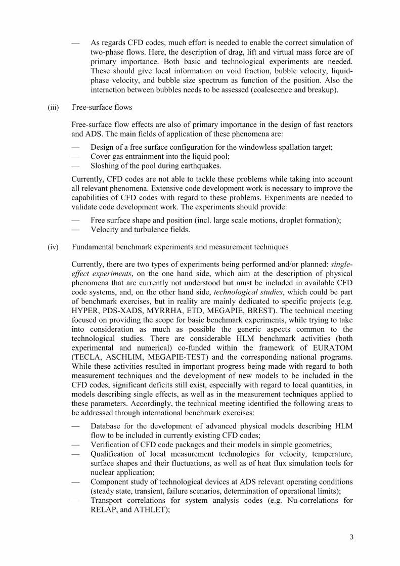
(iv) Fundamental benchmark experiments and measurement techniques

Currently, there are two types of experiments being performed and/or planned: single-effect experiments, on the one hand side, which aim at the description of physical phenomena that are currently not understood but must be included in available CFD code systems, and, on the other hand side, technological studies, which could be part of benchmark exercises, but in reality are mainly dedicated to specific projects (e.g. HYPER, PDS-XADS, MYRRHA, ETD, MEGAPIE, BREST). The technical meeting focused on providing the scope for basic benchmark experiments, while trying to take into consideration as much as possible the generic aspects common to the technological studies. There are considerable HLM benchmark activities (both experimental and numerical) co-funded within the framework of EURATOM (TECLA, ASCHLIM, MEGAPIE-TEST) and the corresponding national programs. While these activities resulted in important progress being made with regard to both measurement techniques and the development of new models to be included in the CFD codes, significant deficits still exist, especially with regard to local quantities, in models describing single effects, as well as in the measurement techniques applied to these parameters. Accordingly, the technical meeting identified the following areas to be addressed through international benchmark exercises:

— Database for the development of advanced physical models describing HLM flow to be included in currently existing CFD codes;

— Verification of CFD code packages and their models in simple geometries; — Qualification of local measurement technologies for velocity, temperature,

surface shapes and their fluctuations, as well as of heat flux simulation tools for nuclear application;

— Component study of technological devices at ADS relevant operating conditions (steady state, transient, failure scenarios, determination of operational limits);

— Transport correlations for system analysis codes (e.g. Nu-correlations for RELAP, and ATHLET);

3

— Identification of the physical effects those are relevant in technological configurations.

With regard to single-effect experiments, the technical meeting identified the following topics as being the most important ones to be covered in such experiments:

— Heat transfer experiments, both in HLM, and also in fluids with the same Pr-number, and considering the following conditions:

(i) Forced convective flow; (ii) Mixed convective flow;

(iii) Buoyant flows; (iv) Thermal shear flow instabilities;

— Free-surface flow phenomena, more specifically:

(i) Stability of the free surface; (ii) Position of free surface as a function of flow parameters;

(iii) Free surface heat transfer capability;

— Two-phase flow effects, more specifically:

(i) Rise of single bubbles; (ii) Form of single bubbles;

(iii) Mixing and coalescence of bubbles; (iv) Void fraction modeling.

3. RECOMMENDATIONS

The technical meeting formulated the following recommendations, expressing the view that their implementation would greatly support the efforts of the HLM R&D community in the various applications currently under consideration:

(i) HLM thermal hydraulics experiments being currently pursued should be brought to the level allowing their use as benchmarks. A coordinated pre- and post-analysis effort of selected experiments is essential.

(ii) Existing and planned experiments (e.g. HYPER, PDS-XADS, MYRRHA, ETD, MEGAPIE, BREST, etc) should be thoroughly evaluated with regard to their relevance as HLM thermal hydraulics benchmarks.

(iii) Best practice guidelines need to be formulated on the basis of knowledge available to enable users to select the suitable turbulence model from the catalogue of those available in commercial CFD codes.

(iv) Commercial CFD code developers must incorporate anisotropic modelling. (v) The HLM thermal hydraulics community should evaluate the newly available

combined turbulence models in some CFD codes. (vi) Suitable modelling to deal with thermal stratification should be included in

commercial CFD codes. (vii) Adequate formulations for the turbulent Prandtl number should be made

available in commercial CFD codes. (viii) Although the technical meeting has considered only CFD issues, it is recommended to

prepare the ground for the integration of CFD codes with all other codes needed for HLM systems development work, e.g. system codes, containment codes, stress analysis codes, etc.

4

(ix) The CFD code users should make use of existing grid computing resources, e.g. within GRID Computing.

(x) It is recommended to define and carry out appropriate benchmark exercises (as the consequence of a verification matrix) in conjunction with international experts groups.

(xi) It is recommended that the single effect experiments cover the following areas: — Heat transfer experiments (both in HLM and in fluids with same Prandtl-number)

in forced convective flow, mixed convective flow, buoyant flow, and thermal shear flow instabilities;

— Free-surface flow phenomena, specifically: stability of the free surface, position of free surface as a function of flow parameters, free surface heat transfer capability;

— Two-phase flow, specifically: rise and downward entrainment of single bubbles, formation of single bubbles mixing, coalescence and break-up of bubbles, void fraction modeling;

(xii) For future single effect experiments it is recommended to adopt the following guidelines: — Provide well-defined experimental conditions (inlet/outlet, geometry, structures,

etc.); — Ensure high degree of instrumentation, high degree of symmetry, and significant

effects to be measured; — Strictly concentrate on the investigation of single effects.

(xiii) The definition of the requirements for instrumentation/diagnostics, and the development of an instrumentation/diagnostics strategy should be, right from the beginning, part of the development and design of the experimental program.

(xiv) The development and design of the experiments and of the instrumentation/diagnostics strategy should also involve CFD and systems codes experts. Their involvement, e.g. in pre-test calculation exercises, is a way to further broaden international participation and ensure close collaboration between the HLM thermal hydraulics R&D community and the code developers.

(xv) Experts on HLM coolant technology should be involved in the design and development of HLM experiments to ensure that potential problems associated with the use of HLM are avoided (e.g. plugging by containments).

(xvi) It is recommended to perform scaling analysis and assessment of scaling distortions with help of dimensionless groups and pre-test simulations.

(xvii) Consideration should be given to the creation of a database to which the experimental data are contributed (basic requirements: format for identification of each sensor, its location and other information, use of EXCEL or other accessible file formats/data banks, data/information readable by all parties, etc).

(xviii) Considering the ongoing projects, it is recommended to give high priority to benchmarks in the area of: — Two-phase flow for pressure mitigation in pulsed spallation targets (ESS); — Free-surface flow for the windowless ADS targets;

(xix) The technical meeting underlined the importance of international collaboration, highlighting the following areas where both the need for international collaboration and the potential gain from international cooperation and coordination are high: — The implementation of an international “fundamental HLM benchmark

experiment and its analysis”, to be performed in the laboratory of one of the participants with the support (e.g. staff, test sections, instrumentation, pre- and post analyses CFD calculations, etc) of the other participants;

5

— The extension of existing databases, specifically the IAEA ADS R&D Database, with the objective of making it suitable to be used by CFD code developers for validation purposes;

— The transfer of the knowledge obtained within the frame of the various HLM R&D efforts to other liquid metal application fields, e.g. metal casting, material processing, semi-conductor production, etc.

6

SESSION 1

REVIEW OF THE STATES OF ART OF PRESENT CDF CODES

TURBULENCE MODELING ISSUES IN ADS THERMAL AND HYDRAULIC ANALYSES

G. GROETZBACH Forschungszentrum Karlsruhe (FZK), Germany

Abstract

Accelerator Driven nuclear reactor Systems (ADS) have in several respects a prototypical character of the flow and cooling conditions combined with narrow operating conditions due to the materials engaged. E.g. the high local thermal load in the liquid metal cooled spallation target requires a very careful analysis by experimental and numerical means. Some of the main goals of the numerical analyses of the thermal dynamics of those systems and of required experiments are discussed. The prediction of locally detached and recirculating flows suffers from insufficient turbulence modeling; this has to be compensated by using prototypical model experiments, e.g. with water, to select the adequate models and numerical schemes. Some sensitivities and model uncertainties are discussed; some of them are reduced by so-called layered models like in the SST turbulence model or the DES. The well known problems with the Reynolds analogy in predicting the heat transfer in liquid metals requires prototypic liquid metal experiments to select and adapt the turbulent heat flux models. The uncertainties in liquid metal experiments cannot be neglected; so it is necessary to perform CFD calculations and experiments always hand in hand and to develop improved turbulent heat flux models. One contribution to an improved 3 or 4-equation model is deduced from recent Direct Numerical Simulation data. Of course, the ADS community would need such extended heat flux models, but even realizing standard 3- or 4-equation ASM heat flux models in the commercial CFD codes would allow for an improved heat transfer modeling, especially when buoyancy is involved.

1. INTRODUCTION

Transmutation is considered a promising technology for significantly reducing the amount of highly radioactive waste. One of the designs of a transmutation reactor is the Accelerator Driven System, ADS, in which a spallation target and an accelerator are used to produce the missing neutrons for the weakly sub-critical reactor, called blanket, by a proton beam [1]. The protons are injected into the spallation target through a vacuum beam pipe that is closed at the end by a beam window, see Fig. 1.

heatexchanger

acceleratorproton beambeam pipe

target module

blanket

beamwindow

Pb or Pb-BiPb-Bispallation

ar a e

FIG. 1. Flow paths through the components of an ADS.

9

The issues in designing and analyzing local details in such a liquid metal cooled nuclear reactor are manifold: one needs detailed methods to describe the momentum and heat transfer to get the local maximum temperature e.g. in simple channels like in the piping system or annular channels, including forced, mixed, and buoyant convection. More complicated channel geometries need to be treated in the fuel elements with the axial flow between the fuel pin bundles and with the cross flow through the heat exchanger bundles. The detailed analysis of the locally time-dependent flow through the thermally stratified large pool areas gains increasing interest because of the thermal striping phenomenon which causes thermal fatigue in the structures; similarly it may be expected that the instantaneous pressure fluctuations in the heavy fluid could also lead to some mechanical problems. Similar problems have also to be investigated in T-junctions of the piping system. And the heat transfer by purely buoyant convection within the complete reactor system has to be considered for some decay heat removal situations, or in some rector concepts even for operating conditions.

Some of these thermal and hydraulic issues are obvious from considering the target. The proton beam will have some MWs that are deposited in a fluid volume of a few liters only. Thus, there are high thermal loads in such liquid metal cooled targets and the type of flow and cooling conditions are quite prototypical. In addition the technological challenges in working with Pb-Bi as spallation fluid needs a lot of development and testing to allow for the design of a target that can safely and reliably be operated. This requires a careful analysis by experimental and numerical means.

The steps which are in principle chosen by the international ADS research partners to develop an ADS target are explained in Ref. [2]: Loops are developed operating with Pb-Bi for the development of the special liquid metal cooling technology [3], and the related measurement techniques [4], to investigate the chemical interactions of the materials and develop new materials [5], to determine in single effect experiments the most important data for improvement of the required turbulent heat transfer models [6], and to analyze in larger loops complete target components or modules to demonstrate and validate the proper design [7, 8]. Supplemental water experiments are performed where more information is required on the velocity field [9, 10]. In parallel the Computational Fluid Dynamics tools (CFD), which are required for detailed heat transfer analyses [11–14] are investigated regarding their suitability for adequate predictions [15, 16], and model developments are ongoing basing on turbulence data from Direct Numerical Simulations (DNS) [17].

All these results are coming together in a project in which a model target, MEGAPIE, is developed and built [18]. It will be operated and irradiated at PSI in Switzerland at the SINQ accelerator, and will also be dismantled and decommissioned at the end. This model target has all prototypical features of an ADS target as shown in Fig. 1, except that the fluid and vacuum side of the target are exchanged, see Fig. 2.

Finally all the experimental and numerical data are used to investigate the heat transfer in an ADS reactor mainly by system codes and by CFD tools. Due to this key role of CFD in scaling up the results from model investigations to reactor applications and due to the narrow window of operating conditions for the allowed velocities and temperatures, a high accuracy and reliability of the CFD codes is required in nuclear reactor hydraulic and thermal analysis.

10

Bypass flow guide tube

Main flow guide tube

Inner beam window

Window cooling jet nozzle

1 MW proton beam

FIG. 2. Window and spallation zone in the MEGAPIE target.

The objectives of this contribution are to extend the discussion of the development procedure of a target in to the modeling issues in the ADS development [2]. The discussed special problems in the current CFD tools are related to the velocity field calculation, like (a) the not sufficiently accurate numerical predictions of a detached flow as it may occur in an ADS target, or (b) the strong deviations in stagnation point flow calculations for the target window for which water experiments are ongoing to select the adequate turbulence models. In a short chapter (c) the status of CFD regarding axial bundle flow predictions is discussed. The problems in calculating the temperature field are related to (d) that the turbulent heat transfer models basing on Reynolds analogy are not sufficiently accurate for liquid metals, which is demonstrated by two benchmark results; (e) this is found to be a serious problem especially for the large scale mixing by the buoyancy influenced flows in large plena. Finally (f) the ongoing model development activities basing on theoretical methods and DNS data are used to gain more accurate turbulent heat transfer models that avoid the Reynolds analogy.

2. MODELING ISSUES IN FLOW DISTRIBUTION PREDICTIONS

The calculation of the velocity field with sufficient accuracy should not be an ADS-specific problem, because in forced convection only the Reynolds number enters into the similarity analysis of the hydraulic problem. Nevertheless, one should get acquainted with the behavior of the current codes. This is required, because in the last years there was a change in the basic CFD tools used in the nuclear community: Several years ago mostly research codes were used, like AQUA, FLUTAN and TRIO, which were usually adapted in their physical models to the requirements of the nuclear applications and which were tested intensively in related benchmark comparisons. Meanwhile, mainly commercial codes are applied like CFX, FLUENT or Star-CD; those codes are multi-purpose codes that are not adapted to the special requirements of liquid metal heat transfer.

In order to gain experience with these codes and to find their practical limitations in ADS applications, a European Concerted Action was performed for the Assessment of CFD codes for Heavy Liquid Metals (ASCHLIM), in which benchmark calculations were performed and in which so far as possible the results were compared to experimental data [15] to find conclusions for the required model developments. Here we use published results of our FZK contributions to some benchmarks in ASCHLIM, combined with the results of additional investigations of target relevant flows from [2], to extend our conclusions on the required model developments and qualification on the hydraulic side, and on the thermal side in the next chapter, which are required for a successful detailed ADS analysis.

11

2.1. Detached flow predictions

The modeling issues on the fluid dynamics side of the ADS target development are due to the fact, that the flow geometry, which is optimized for the window cooling, may cause flow separation. This could be expected in the diffuser-type widening of the cross section around the window, see target sketch in Fig. 1. As it is well known that the standard k-ε turbulence model, which is the basis of most commercial and research codes, has serious problems in predicting the existence and extensions of detached recirculating flow areas [19], the benchmark WP3 was performed within the ASCHLIM project, in which the isothermal flow around an ADS typical target window had to be predicted and compared to data from the COULI water experiments [10]. In the preparation of this benchmark blind predictions for the experiments were performed by some of the partners. The geometry specifications are given in Refs [15, 20] in which also details of our blind predictions are presented.

The calculations were performed with the FLUTAN code that was developed at FZK [21, 22]. It is a code to simulate single-phase flows with heat transfer of several fluids with small compressibility in complex geometries using structured rectangular grids with additional discretization features like local grid refinement and body fitted grids. Several turbulence models are available in FLUTAN like models based on transport equations for some turbulence quantities. Two cases, one for a small Reynolds number at the inlet, Re = 2×104, and one for a realistically high one, Re = 9×105, were given. The water temperature is 60°C. Most calculations were performed with the standard k-ε turbulence model and with a first order upwind method of the convective terms in the equations for the momentum and turbulence quantities. The system of equations was solved on a structured rectangular grid.

The results for the high Reynolds number case are presented in terms of the calculated modulus of the velocity vector in the plotting plane normalized by the inlet velocity into the funnel, see Fig. 3.

FIG. 3. FLUTAN results for the COULI benchmark: Modulus of the velocity vector normalized by the axial inlet velocity Win, Re = 9×105.

12

FLUTAN simulates very low velocity values with a flow detachment at the inner wall downstream of the beam window. Calculations with second order discretisation methods like QUICK and LECUSSO were likewise performed with the same grid. The length of the recirculation zone increases downstream in going from first to second order schemes. However, a qualitative influence from the discretisation method on the occurrence and on the size of the recirculation zone can only be avoided when adequate iteration parameters are used as the higher order schemes need sharper criteria. All results are fully converged calculations and show a flow detachment at the inner wall.

The reliability of this result is doubtful because the standard k-ε model uses wall functions to approximate the wall shear stresses, but wall functions are not valid near stagnation points and in the detached flow area. Therefore, turbulence models without wall functions must be used for this case. Calculations for the smaller Reynolds number with a low-Reynolds number k-ε model, which contains additional terms in the transport equations for k and ε for the near wall area, do not need wall functions, but require fine grids near walls. Such calculations with FLUTAN show velocity fields with a strong reduction of the size of the detached area at the inner wall, but at the same time the area with small velocities increased at the outer wall, so that there may be a tendency to develop also a detached flow at the outer wall. However, this result is not representative for a reliable analysis because the used grid is near the walls too coarse for this kind of turbulence models.

The pre-test results from other codes presented at the first benchmark discussion showed in some cases the detached area not at the inner wall, but at the outer wall. Star-CD gave with a low-Reynolds number model at the larger Reynolds number the detached area near the outer wall and for the smaller Reynolds number in addition one near the inner wall. Finally, in the experiment a flow separation was found at the outer wall [10]. The pre-test calculations showed that no computer code participating in the COULI benchmark could reliably “predict” the location and the extension of the flow detachment at least with the used models. And even the post-test calculations showed that the physical models have to be carefully selected to gain acceptable results [15]. Therefore, already without heat transport a complex interaction turns out between physical models and code-dependent numerics in the simulation of typical ADS target flows which at the current status of the two-equation turbulence models always requires accompanying experiments which should provide detailed velocity and turbulence field information for choosing adequate models and for validation.

2.2. Recirculating flow predictions

Extensive recirculation is appearing in the MEGAPIE model target which is developed in an international cooperation and which is now under construction [18]. This model target has all important features of a typical ADS target except the vacuum and spallation sides are exchanged; see Figs 1 and 2. In MEGAPIE the downward flow in the annulus and the upward flow inside the guide tube are combined with a sideward flow across the window to remove the stagnation point from the hottest zone by using a nozzle to produce a jet flow across the beam window. In the conceptual design phase of the MEGAPIE target, several design concepts were proposed for effective cooling of the window and the target itself [13, 14]. In the first design configuration there is no bypass injection and the guide tube is cut horizontally. The numerical work by using CFX 4 and CFX 5.5 is focused on this first configuration that also was the topic of the first HYTAS experiment series [9]. The detailed specifications and computational results are summarized in [23].

The flow domain is geometrically axisymmetric. With axisymmetric inlet conditions and boundary conditions, a two-dimensional flow would be expected. Three different kinds of

13

computational configurations are selected, i.e. a 2D axisymmetric one, which is discussed here, a 3D half-scale (180°), and a 3D full-scale (360°) configuration. Five turbulence models are selected to assess their effect on the calculated velocity field, the k-ε, RNG k-ε, low-Re k-ε, k-ω and the SST model. The SST turbulence model (Shear Stress Transport) is a layered version of the k-ω model in CFX 5.5.1 [24]. Coupled with the turbulence models, the mesh sizes of the structured grid in the near wall region are adapted adequately. The flow Reynolds number is 10 000, where Re is based on the mean velocity and hydraulic diameter in the annular gap. The thermal properties of water at 20°C are used.

The axial velocity component W calculated with the standard k-ε model shows downward flow not only in the annular downcomer, but also near the centre of the widow and inside the guide tube near its lower end, see Fig. 4.

< 0.0

0.5

0.25

m/s

z

FIG. 4. Axial velocity W in half of a MEGAPIE target without bypass jet, standard k-ε model, Re = 104. Blue areas indicate zero velocities or downward flow (to the left).

The recirculation zone in the guide tube concentrates the upward flow into a narrow area around the axis of the target. With increasing height z the cross section that is available for the upward flow is increasing so that the maximum of the axial velocity component is decreasing. The maximum axial velocity values that are predicted by the five different turbulence models differ by about 10%, see Fig. 5.

0,0 0,2 0,4 0,6 0,8 1,0

-0,2

-0,1

0,0

0,1

0,2

0,3

0,4

0,5

0,6

STD k-ε RNG k-ε Low Re k-ε Low Re k-ω SSTW

[m/s

]

z [m]

FIG. 5. Axial velocity W along the vertical axis of the jet-less target calculated with different turbulence models, Re = 104.

14

However, there exist significant qualitative differences in the flow fields near the window centre and in the region downstream around z = 0.4 to 0.8 m. Near the window the SST turbulence model doesn’t predict any recirculation while the other turbulence models do. In the region downstream of the lower guide tube end, large differences in the flow fields exist. The steeper decrease of the axial velocity, which is at the upper end of the recirculation zone at the inside of the guide tube, is at different axial positions. This shows that the different turbulence models predict very different axial extensions of the recirculation area. In the target this recirculation would be exactly on the height of the spallation zone; therefore, these differences could have strong consequences on the calculated temperature distributions.

Thus, detailed experimental data for the velocity field and some turbulence data in the prototypic geometry with jet are strongly required for the selection of an adequate turbulence model and its validation, especially in certain regions, i.e. near the window and between z = 0.4 and 0.8 m. Other parameters, like the chosen mesh or the size of the computational domain, have compared to this sensitivity only a weak influence on the predicted results. It is shown that the type of the advection scheme has a strong influence on the temperature filed; as the advection scheme is influencing the temperature by means of the velocity field, the selection of an adequate scheme should be performed on the basis of velocity data from such detailed water experiments [25]. Performing the HYTAS experiments was found to be rather challenging. Therefore, there are currently no direct comparisons to the experimental data possible.

2.3. Other issues in flow field predictions

There exist no universal turbulence models that could be used for any type of turbulent flows at any Reynolds number. Therefore, our CFD codes provide a list of different models from which the user has to select the suitable one. One important difference occurs in the different modeling approaches in the near-wall area. Standard models use wall functions to calculate the wall shear stresses in the mean flow direction. With these models it is not required to use very fine grids near the wall to resolve the viscous sublayer; just the opposite is required: the grids must be coarse enough so that logarithmic wall functions can be applied. So, these models are the preferred ones for high Reynolds number flows, but they are not valid e.g. for detached and recirculating flows, because we do not have adequate wall functions for such flows. For detached flows one prefers the so-called low-Reynolds number models which need to resolve the viscous sublayer, but which then need special near-wall adaptations in the transport equations of the turbulence models. Those adaptations are expected to be more universal than the wall functions. So, such models are the preferred ones for flows at lower Reynolds numbers, or on powerful computer systems also for computations for somewhat larger Reynolds numbers. Of course, in practice there is a large sensitivity found in switching between these models and the adequate grids, which always requires verifying the calculated data on experimental data. So, what is needed is to achieve less sensitivity against this selection of the models. Or, as it is realized now in CFX 5, to develop intelligent methods which use a kind of blending between the different types of models so that this sensitivity can strongly be reduced because the resulting turbulence modeling, called SST [24], can be applied for a wide Reynolds number range.

The statistical turbulence models basing on the time-averaged Navier-Stokes equations, called Reynolds-Averaged Navier-Stokes models (RANS), are not the adequate tool when the consequences of the high energy containing low frequent turbulence has to be investigated, e.g. the consequences of thermal striping or of the pressure fluctuations in fluid-structure interaction. For such investigations Large Eddy Simulation (LES) is increasingly used which

15

simulates directly the large scales of turbulence and models by sub-grid scale models (SGS) only the small scales that cannot be resolved by the grid [26]. The results of such LES are in principal less sensitive against modeling assumptions; nevertheless, there exist also no universal SGS models and no universal wall modeling. Thus, we find in these promising field similar challenging problems regarding the universality of the models, regarding their applicability to near wall flows at all Reynolds numbers, and regarding the wall treatment. An attractive compromise, which was recently developed to avoid part of these problems especially for flows around air foils, is the Detached Eddy Simulation (DES), which combines low-Reynolds number RANS modeling near the walls and Large Eddy Simulation apart from walls [27]. This DES may also be a powerful method to investigate low-frequent time-dependent phenomena in an ADS. The method is realized in the actual CFX 5 version. What hinders usually the wider application of LES or DES is that one needs finer grids and more time steps to get sufficient data, and that in channels with an inlet and an outlet it is hard to specify meaningful time-dependent turbulence at least at the inlet. So, more efficient methods are required to provide suitable inlet data.

All these issues in modeling and calculating velocity fields are not ADS specific. Some of them are known since decades and could not be solved by the turbulence modeling community despite tremendous research. So, it is not expected that the ADS community could seriously contribute to new solutions. Thus, if one has to treat one of these problematic cases one has always carefully to select the adequate modeling by checking the results of the chosen method by means of experimental results for the underlying flow regime or by means of experimental data directly for this prototypical flow. Of course one should consider using the recent combinations of methods like the SST and the DES that are especially intended to reduce or even to avoid some of the general problems. Finally, these or similar combined models which should have a wide range of applicability should be made available in all typically applied CFD codes.

2.4. Development needs for bundle flow predictions

The fuel element analysis is an important application field; therefore, some specific requirements for calculating the axial flow through fuel bundles should be discussed shortly. There are already applications of CFD to study heat transfer in bundles [28] or even to optimize mixing vanes at the spacers of reactor fuel elements [29]. By using different variants of the k-ε model and a full second order closure model it was found that the k-ε models give more or less insufficient accuracy for the bundle flow, that some of them give good secondary currents (which are the induced flows in the plane perpendicular to the axial mean flow), and that the second order model gives better results. It is concluded, that the used models are inadequate to capture the anisotropy and that other models should be investigated or new models should be developed. To analyze this conclusion we shortly discuss what is known from historical experiments in bundle flows and from former numerical analyses.

Basic experiments with detailed flow, heat transfer, and turbulence measurements in bundles were performed at FZK between the eighties and the mid nineties, see e.g. in [30]. These experiments, in which e.g. the gas flow through a large 4-rod arrangement in a rectangular channel was investigated, are still the basis for code benchmarks. The main results which are of interest if one decides to use CFD are that the flow is strongly anisotropic, especially in the near wall zones, that the expected secondary currents are near the measurement accuracy and can therefore hardly be detected. In addition systematic periodic oscillations were found in the spanwise velocity components and in the pressure in densely packed bundles which cause intensive mixing between subchannels [31].

16

First experiences with numerical analyses of axial bundle flows were basing on two-dimensional mixing lengths approaches. It is found that such flows need at least the use of anisotropic eddy diffusivities to reproduce bundle flows adequately; especially the azimuthal turbulent diffusion of momentum and heat near walls needs special care [32, 33]. It is found that bundle flows need the modeling of the secondary currents to get the correct azimuthal variation of shear stresses and heat fluxes [34]. It is shown by means of LES that eddy diffusivities are a transportable quantity and that they are considerably influenced by secondary currents so that only transport equation models will have a chance to record adequately flows with secondary currents [35]. If densely packed bundles have to be considered, the highly intermittent periodic oscillations coming from the transport of coherent structures in the narrow gaps between fuel pins can well be treated by LES [36].

So, one has to expect that successful CFD applications can nowadays only be performed if the user of the CFD code is aware of the problematic physical background so that he can select the adequate models. From our nowadays knowledge we have to conclude that anisotropic turbulence modeling is required whereas the secondary currents are smaller than expected; they are usually automatically reproduced in a three-dimensional CFD. This means, it is known that there is no chance to record axial bundle flows with any isotropic eddy diffusivity and eddy conductivity model, i.e. all isotropic or standard k-ε models will fail. One has to use at least good Algebraic Stress Models (ASM) or sophisticated second order models. And for the strong inter-subchannel mixing in densely packed bundles one has to use either LES or DES. Whether the existing models are really sufficient, or whether further development of them is needed, cannot be deduced from the available investigations.

3. MODELING ISSUES IN TEMPERATURE DISTRIBUTION PREDICTIONS

3.1. Reynolds analogy and liquid metal heat transfer

To realize the challenges that we face when doing heat transfer predictions for liquid metal flows with RANS methods one should consider what are the methods that we use in our CFD tools on the momentum transfer side and on the heat transfer side. The conservation equations for mass, momentum, and thermal energy do not form a closed set of equations if the statistical or Reynolds approach is used to describe turbulence. In fact, unknown correlations between velocity fluctuations ui and uj called turbulent shear stresses jiuu and between velocity fluctuations and temperature fluctuations θ called turbulent heat fluxes θiu exist in these equations. These terms that represent the turbulent transport of momentum and heat have to be modeled.

A widely used class of turbulence models is based on the eddy viscosity/eddy heat diffusivity concept [37]. The eddy viscosity νt and eddy heat diffusivity Γt are respectively introduced by a mean gradient approach in terms representing the turbulent transport of momentum and heat. There was already tremendous research in how to model the eddy viscosity for the turbulent momentum transport. It is usually approximated by using any variant of the k-ε model. The much more complicated and nevertheless less investigated eddy heat diffusivity is approximated mostly much less sophisticated; it is assumed to be also isotropic and to be linked to the eddy viscosity by a fixed turbulent Prandtl number Prt = νt / Γt . This implies that the turbulent transport of heat is assumed to be strictly analogous to the turbulent momentum transport. These assumptions are the basis of the Reynolds analogy. This analogy works well for a wide class of flows but not for liquid metal flows. Due to the strongly different values of the relatively small molecular viscosity ν and the relatively large thermal diffusivity Γ, the statistical features of the turbulent velocity and temperature fields are not similar, like it is

17

indicated by the different thicknesses of the molecular wall layers or the differing positions of the fluctuation maximal of the velocities and temperatures. This means, the Reynolds analogy should not be applied because it has no basis for fluids with small molecular Prandtl numbers Pr = ν/Γ. At least for these fluids the turbulent Prandtl number is no longer a fixed value, but it depends on a number of parameters like Pr, Re, and wall distance [38, 39]. As the turbulent Prandtl number at all Pr below one is found to increase strongly near walls, and as the near-wall area is at a heated wall the most important area in heat flux modeling, any concept of using a spatially constant value of Prt will lead to insufficient results; nevertheless, this is the status quo of our current CFD tools in modeling liquid metal heat transfer.

In contrast to this modeling, formulations should be used which approximate the turbulent eddy conductivity Γt in liquid metals independent of νt, like in the first order 4-equation model [40]. Such 4-equation models based not only on k- and ε-equations, but in addition on transport equations for the temperature variance 2θ and its dissipation or destruction θε , allow also for different time scales in the turbulent velocity and temperature fields.

For buoyant flows one gets strong anisotropy in the turbulence field due to the orientation of the buoyancy force. In such flows even a second-order description of the turbulent transport of heat should be applied, which means the use of independent transport equations for the three components of the turbulent heat flux vector. Such models are not constrained by any of the above-mentioned problems. Therefore, in order to simulate turbulent flows in liquid metals with buoyancy influences it is reasonable to use a second-order model at least for the turbulent transport of heat. The Turbulence Model for Buoyant Flows (TMBF) [21, 41] which is developed and implemented in the CFD Code FLUTAN [22] belongs to this class of models. It is suitable for the simulation of the turbulent transport of heat in liquid metals because it uses a second order model for the turbulent heat transport with special model extensions. The model extensions are widely basing on DNS data [42, 43].

Similar turbulent heat flux models are missing in the commercial CFD tools that use at least some transport equations for statistical features of the thermal field. So, one has to live with the uncertainties of the Reynolds analogy, has to investigate from application to application which formulation for the turbulent Prandtl number is the more suited one, and has to verify carefully the finally computed results by comparisons to directly related liquid metal heat transfer experiments.

3.2. Heated annulus heat transfer predictions using Reynolds analogy

Here the limits of our current CFD capabilities are investigated by applying the Reynolds analogy to an experiment in our KALLA laboratory [44]. We use an annulus with a heated inner rod cooled by flowing liquid Pb-Bi. More detailed specifications and experimental as well as numerical results are given in [6, 45].

The rod with an outer diameter of d = 8.2 mm is installed concentrically in a pipe with D = 60 mm inner diameter in the THESYS loop of the KALLA laboratory. The rod has a total length of 2 500 mm, the heated length is 228 mm. The rod can be traversed axially in z-direction by 240 mm to measure with the radially traversable Pitot probe and thermocouple at different axial positions relative to the begin of the heated length, see Fig. 6.

18

FIG. 6. Heated rod experiment in the KALLA loop.

The helical Inconel heater inside the rod is DC current heated. In this experiment a maximum surface heat flux of q’’ = 34 W/cm2 was used. The inlet temperature is Tin = 300°C. This corresponds to a molecular Prandtl number of the fluid of Pr = 0.022. The mean Reynolds number in the pipe zone basing on mean velocity and hydraulic diameter is Re = 105.

The calculations have been performed using CFX 4.4. 2D and 3D structured grids were applied. Special attention has been paid to keep the first grid point from the wall in the range of 30≤y+≤50 because this is on one hand side required to work with wall functions in the velocity field; on the other hand side this is still in the conductive wall layer, so that it can be avoided to apply the thermal wall function formulation which is in this code version inadequate for liquid metals. The standard k-ε model has been used and the turbulent Prandtl number has been set to Prt = 0.9. A first order hybrid scheme has been selected for the advection terms. In order to examine the effect of buoyancy 3D calculations were performed including the full developing length of the flow as in the experiment. The thermal insulation has been taken into account using a constant temperature at the outer boundary.

The results of the first experiment series were the basis of ASCHLIM benchmark WP 4 [15]. The comparison of these results with the computational results leads to considerable discrepancies in the temperature field near the heated wall [45]. So, a systematic investigation was performed to learn about the most sensitive uncertainties in the modeling. By changing the effective thermal conductivity in the insulation in the calculation it could be excluded that support structures going through the insulation could have a considerable influence. By changing the turbulence level at the inlet into the computational box its influence could be excluded because with altered data the measured velocity profile could not be reproduced. Serious problems with an inadequate turbulent Prandtl number could be excluded because in increasing this value the deviations even increased. The near wall resolution was adequate because a further refinement had no effect on the results. And switching over to a low Reynolds number turbulence model and adapting the grid in the required manner lead to the same temperature profiles. With the full 3D calculation it could finally be excluded that buoyancy influences the results at this Reynolds number. Thus, after intensive discussions of possibly missing phenomena in the calculations and of possible uncertainties on the test section side it was expected that the fixation of the rod was not sufficient to avoid that an eccentricity of the rod in the pipe may have been built due to the swimming up of the light rod in the heavy fluid in the horizontal channel. So the construction of the test section was changed and additional spacers were introduced.

19

The new experiment series shows much better radial temperature profiles if one takes the data from the thermocouple array below or beneath the rod [6]; the data from above the rod indicate that the temperature field is still not fully axisymmetric. The originally calculated numerical results are now in much better agreement with the new experimental data, see Fig. 7.

0 0.01 0.02 0.03radial position [m]

0

10

20

30

40

50

tem

pera

ture

rise

[°C]

all TE rakes except topExperimentFit : PowerCFX

T - T i

n

r

FIG. 7. Measured and calculated radial temperature profiles at half heated length of the heated rod experiment, Re = 105, q’’ = 34 W/cm2.

Nevertheless, the agreement is not perfect: The computed fluid-wall interface temperature is for all axial positions larger than the measured one, e.g at half of the heated length by about 10%. The deviation would increase if more realistic turbulent Prandtl numbers with values above one would have been used; but this would not help to bring the calculated profile around r = 0.01 m nearer to the measured one.

This benchmark indicates that heat transfer investigations for Pb-Bi have considerable uncertainties on both sides, on the numerical as well as on the experimental side, even if simple channel configurations are used. The measured temperature profiles cannot be reproduced by using a constant turbulent Prandtl number; at least a radially varying value should be used to achieve a better agreement. To adapt higher order turbulent heat flux models requires additional experimental data for velocity-temperature cross correlations which can currently hardly been provided. On the other hand it gets obvious that not only CFD needs assistance, here by experiments, for quality assurance, but also vice versa the quality of experiments profits considerably from parallel CFD analyses.

3.3. Heated jet heat transfer predictions using a second order turbulent heat flux model

A number of experiments in literature provide data for time mean temperature fields in turbulent liquid metal flows, but reliable turbulence data of the temperature field in liquid metal flows are rare. Such data are required to investigate the performance of more sophisticated turbulent heat flux models basing on transport equations. One data set, that was already once used in an IAHR benchmark is the one of the TEFLU experiments [46]. There, the turbulent mixing of momentum and heat was investigated in the co-flow of a multi-jet arrangement using liquid sodium, Pr = 0.006 [47], see Fig. 8.

20

ΔU ΔT

U TCf Cf

D= 110 mm

d= 7.2 mm

x

r

FIG. 8. TEFLU geometry with a heated sodium jet in the co-flow from a multi-bore jet block.

Some of the TEFLU data were chosen also in ASCHLIM in work package WP 2 to investigate the performance of some codes and their models [15].

Here we show results that we got by using the latest version of the TMBF model [21]. This is a combination of a low-Reynolds number k-ε model and a second order turbulent heat flux model consisting of the transport equations for the three heat fluxes, for the temperature variance 2θ , and for its dissipation θε . The calculated turbulent stresses and heat fluxes are not related through a fixed turbulent Prandtl number Prt. Thus the TMBF represents a compromise between the classical k-ε-Prt model and a full Reynolds stress model. In addition, the TMBF contains a number of special model extensions for liquid metal heat transfer which were deduced by theoretical means and by using our DNS data for liquid metal buoyant convection [48].

The extended modeling is verified at small Prandtl numbers without and with buoyancy contributions by means of some TEFLU experiments. Using a free jet experiment in a highly turbulent multi-jet surrounding to analyze the performance of turbulence models has the advantage that the results are mainly governed by the turbulence models and do not suffer from any inadequate wall modeling. Three different buoyancy regimes were considered in the benchmark; they were classified as forced jet, buoyant jet, and plume. The FLUTAN calculations applied not only the TMBF but also the standard k-ε-Prt model in order to investigate the advantage of the TMBF compared to the k-ε-Prt model. The specifications of the calculations and a detailed discussion of the results are given in Ref. [21].

The radial temperature profiles predicted by the k-ε-Prt model for the forced jet case are flatter than the measured ones, see Fig. 9.

21

FIG. 9. Forced jet, radial temperature profiles at three different axial positions x/d, measurements and calculations with the k-ε-Prt model (left) and TMBF model (right).

The reason is the over-estimation of the radial heat transport from the axis to the outer flow. The mean temperature field is better predicted by the TMBF. This model calculates a smaller turbulent heat flux in the radial direction than the one calculated by the k-ε-Prt model.

In considering the velocity and temperature profiles for the buoyant jet and for the plume it was found that the results of both models, of the k-ε-Prt model and of the TMBF, agreed quite well with the experimental data. This astonishing result is caused by the fact that the local Reynolds numbers in these cases were too small so that the corresponding temperature fields were mainly governed by heat conduction and were only weakly influenced by turbulent convection. As many technical applications of liquid metal heat transfer are in the transition range between having mainly conduction dominated temperature fields and convection dominated ones, these cases were analyzed in more detail. Indeed, the results of the TMBF for the plume case indicate the need for further improvements in the TMBF model: Whereas the predicted temperature variances for the forced and buoyant jet agree with the experimental data, the results for the plume deviate considerably. So, the focus of further research was on the closure terms in the equations for the temperature variances and its dissipation; see Section 4.

The TMBF uses the full transport equations for the turbulent heat fluxes; thus, it is possible to analyze from its numerical results the turbulent Prandtl number which would be required to produce the same temperatures with the Reynolds analogy. The fields of such calculated Prt reaches values beyond 5, see Fig. 10.

Thus the values are locally much higher than the value of Prt = 0.9 which is usually applied in calculations with the k-ε-Prt model. Moreover, it is not constant. It depends not only on the fluid, but also on the flow regime and on the position. Indeed it was found that the k-ε-Prt model can only give good results by adjusting the value of Prt to reduce the turbulent heat flux perpendicular to the flow direction [41]. This is consistent with the findings of other partners in the ASCHLIM project that only those results were roughly acceptable which are based on physical models applying at least non-constant turbulent Prandtl numbers. The TMBF results were evaluated to be the most promising ones.

Cal. X/d= 11Cal. X/d= 19Cal. X/d= 39Exp. X/d= 11Exp. X/d= 19Exp. X/d= 39

r [m]

T [ C]0

Cal. X/d= 11Cal. X/d= 19Cal. X/d= 39Exp. X/d= 11Exp. X/d= 19Exp. X/d= 39

r [m]

T [ C]0

22

FIG. 10. Turbulent Prandtl number Prt calculated by the TMBF model for the forced jet(left),buoyant jet (middle), and plume (right). x-axis in the vertical direction along the centre line starting at begin of computational domain (6d behind jet block), -radial coordinate starting at jet axis.

3.4. Issues in buoyant flow predictions

Flows, which are influenced or exclusively driven by buoyancy forces, like in large reactor pools, have some peculiarities compared to forced flows. One is the fact that in such flows there is not only a coupling from the velocity field into the temperature field equation by means of the convective term, but also the coupling back from the temperature field by means of the buoyancy force into the momentum equation. As a consequence the velocity field is influenced by the Prandtl number and thus detailed experiments to study the turbulence in buoyant flows need model fluids with about the same Prandtl number as the operating fluid for which the investigation is performed. Thus, one is faced with the serious problem of finding sensors to measure e.g. the local turbulence in the velocity field in liquid metals. As there aren’t sufficient possibilities available, DNS is the standard tool to provide the data that are required for model development, see Section 4.

The other important peculiarity is that the turbulence in buoyant flows is not only anisotropic due to the presence of the walls, but also in the complete channel due to the presence of the directional buoyancy force. It is well known that such flows can only be calculated with sufficient accuracy by means of models which use additional transport equations for quantities of the thermal field, like for the temperature variance 2θ and in some cases also for its dissipation or destruction θε [49]. Such 3- or 4-equation models could also be extended to treat the influence not only of augmenting buoyancy but also of damping buoyancy in case of stable stratification.

In using recent DNS data for Rayleigh-Bénard convection in a liquid metal with Pr = 0.025 at a Rayleigh number of 105 we analyzed the turbulent heat flux which would be predicted by a standard k-ε model using a constant turbulent Prandtl number of 0.9 [50], see Fig. 11.

r [m]

X (m)

Forced Jet - TMBF Model

σT

5.04.03.02.01.0

r [m]

X (m)

Buoyant Jet - TMBF Model

σT

5.04.03.02.01.0

r [m]

X (m)

Plume - TMBF Model

σT

4.03.02.01.0

Prt Prt Prt

23

0,0 0,2 0,4 0,6 0,8 1,00,00

0,02

0,04

0,06

0,08

0,10

0,12

0,14 DNS data k-eps-Pr

t

<u3' θ

>

x3

FIG. 11. DNS data for the vertical profile of the turbulent heat flux θ3u in Rayleigh-Bénard convection and for the prediction by a k-ε-Prt model, Ra = 105, Pr = 0.025.

The DNS data for the upward directed heat flux shows thick conductive wall layers, whereas the profile which would be predicted by the Reynolds analogy has a much thinner conductive wall layer and large peaks near the walls. Any other spatially constant turbulent Prandtl number would also give such disastrous predictions, so that this concept is not applicable even for this simple buoyant heat transfer problem. A similar problematic experience was e.g. gained with practical applications of the k-ε-Prt model for the calculation of the cooling conditions in core melts, where it was decided to use DNS or LES instead [51]. So, indeed more extended models are required which base at least on 3 or 4 transport equations for turbulence quantities and which should be combined with ASM extensions to record the anisotropy of all turbulent fluxes. One example for such a new ASM heat flux model with 4 equations which is suited for liquid metal convection is discussed in Ref. [17]; part of its important extensions for liquid metals is discussed in Section 4. Unfortunately, such ASM or second order models which are suited for liquid metal heat transfer are up to now not available in commercial codes.

3.5. Other issues in temperature field predictions

As with the turbulence modeling for the velocity field, we also find that there exist no turbulent heat transfer models that are universal. Especially the additional parameter of the molecular Prandtl number of the fluid leads to large uncertainties for applications to liquid metal heat transfer. Most of the models do not have special adaptations as they are required to include the stronger influences of the molecular conduction in the equations for the temperature variances or the turbulent heat fluxes.

The influence of the molecular Prandtl number occurs also in the wall conditions. The ‘universal’ wall functions for the temperature profile in forced flows depend also on the Prandtl number, and so do also the thicknesses of the conductive wall layers. In liquid metals the conductive wall layer is much thicker than the viscous wall layer. E.g. at moderate Reynolds numbers it may be necessary for usual grids to use wall functions in the velocity field, but it may be possible to resolve with the same grid the conductive wall layer in a liquid metal. It is this fact, which needs separate modeling of both wall layers. Unfortunately this is

24

not correctly treated in most commercial CFD codes, and not all have suitable thermal wall functions for a wide Prandtl number range, so that in some CFD codes, like Star-CD, always coding is necessary to adapt the numerical treatment and the physical models to the ADS typical conditions. This problem is a further argument to use, wherever possible, low-Reynolds number modeling to avoid any problematic wall functions.

A peculiarity occurs e.g. in the stagnation flow at the target window, see Fig. 3. There we have a flow type similar to a wall impinging jet. For this flow type it is known that the turbulent heat transfer from or to the wall strongly depends on the turbulence model for the velocity field. Some k-ε models and even second order models are found to over-predict strongly the local turbulence level. As a consequence a too large heat transfer is predicted [52], so that a series of model extensions are required [53]. Again, this is a field of ongoing research in the turbulence modeling community that is not ADS specific. The CFD code developers follow the development and try to provide models that could also be used with limited success for this flow type. So, one has always carefully to check which one of the available more sophisticated models is really the better compromise.

In applying LES for time-dependent problems, like for the thermal striping phenomenon, the influence of the molecular Prandtl number needs also special consideration [26]. SGS heat flux models also depend on the molecular Prandtl number, but the turbulent Prandtl numbers for RANS models and SGS models are not the same. In considering the energy spectra for velocity and temperature fluctuations one can deduce that for fluids with Pr around one, Prt for the subgrid scales is around 0.45. For liquid metals Prt values can also be deduced from the spectra. Considering that the temperature spectra have vanishing energy at high frequencies with increasing thermal diffusivity or decreasing Pr leads to the result that even on coarse grids nearly all thermal fluctuations are resolved so that with finer grids no SGS heat flux models are required and Prt for the subgrid scales approaches infinity [54]. The arguments regarding the calculation of the wall heat fluxes are the same as for the RANS applications; one should avoid thermal wall functions, what is usually possible in ADS applications.

A further problem that is often underestimated is the verification of the complete setup of the numerical model consisting of the geometry specification, numerical grid, specification of the physical features of the involved fluids and structures and their interaction, and the physical model selection. With available computers one cannot reproduce completely the reality. So, simplifications are always introduced and some phenomena are neglected basing on engineering judgment. This holds also for the selection of the adequate models. The problem gets obvious if one considers e.g. buoyant flows: There one has to select which of the structures do thermally interact with the flow field, so that they have to be recorded, and which of the smaller support structures or instrumentation rods may be of second order relevant and can be neglected. In one example we had to learn that even for common fluids like water the engineering judgment could lead to wrong conclusions on what can be simplified and what has to be recorded in the numerical model because we did not expect that some thin support bolts and cooling pipes going through a large pool had to be recorded in the CFD model to get qualitatively and quantitatively sufficient results [55]. The verification of the assumptions that are done by the code user is the main reason that we will always need prototypical experiments in which a similar combination of the physical phenomena is occurring as in the final technical application. This experiment should be reproduced first by the code user to verify his engineering judgment before going to the prediction of the technically relevant flow and heat transfer problem. Unfortunately the selection of the adequate turbulence models needs some local and very detailed turbulence data of the

25

velocity and temperature field and some cross correlations, so that the instrumentation of such prototypic experiments is also a challenge.

4. ISSUES IN TURBULENT HEAT FLUX MODEL DEVELOPMENT

The results discussed above show that turbulent heat flux models that base on transport equations are superior to the Reynolds analogy using simple turbulent Prandtl number formulations. The challenge in developing the more sophisticated models is that the measurement capabilities are very limited to provide the required detailed local data, especially cross correlations between velocities, pressure, and temperature fluctuations in liquid metal flows. Direct Numerical Simulation of turbulence is the common tool to provide the required data at least for small turbulence Reynolds numbers. Examples for liquid metal forced flows are the data by [40, 56], and for liquid metal buoyant flows those from [43].

Our analysis of the closure terms in the transport equations for the temperature variance and its dissipation is aiming to use DNS data for Rayleigh-Bénard convection in several low-Prandtl number fluids. The required DNS data were not yet fully available because liquid metal simulations need extremely fine grids to resolve the small scales in the velocity field and to record a large computational domain because flow structures with long wavelengths exist in this flow type. The available DNS for liquid metal convection by Refs [43, 57] did not reach sufficiently high Rayleigh numbers to be in a fully developed turbulent regime in the thermal field. Thus a new simulation was performed for a higher Rayleigh number. Starting from earlier simulations in Ref. [57] we ran one with the TURBIT code from Ref. [43] for turbulent convection in mercury or lead-bismuth, Pr = 0.025, at Ra = 100 000. Ra is defined by the channel height D and the temperature difference between both horizontal walls ΔTw. The underlying grid consists of 400×400×75 mesh cells and uses a periodic computational box of 8×8×1 normalized by the channel height. The analyses of the simulation show that this Rayleigh number and even somewhat higher ones can be achieved with current computer systems and that the convection at this Rayleigh number gets now closer to the required fully turbulent regime. The data are used to analyze improvements of the TMBF or of the 3- and 4-equation models for ADS applications.

The statistical analyses of the DNS data show that several of the closure terms in the temperature variance and destruction of temperature variance equations should be the focus of improvements because the existing models lead to insufficient agreement with the data. In earlier work [48, 58] we concentrated on the destruction (or dissipation) of the temperature variance θε . It was found that the standard set of empirical coefficients for this transport equation is not sufficient for getting good agreement with the experimental field of the temperature variances at small Prandtl numbers.

The recent analyses of the DNS data concentrate on the other important closure term in these equations, here especially on the modeling of the turbulent diffusion term 2θii ux∂∂ in the transport equation for the temperature variance [50]. The standard modeling applies the scalar or isotropic Gradient Diffusion Hypothesis (GDH) for the triple correlation:

iSi x

kCu∂∂

−=22

2 θε

θ θ (1)

This is usually the approach when a k-ε model is used. The results are made dimensionless by using the following scaling measures: D is the length scale, u0 = (gβΔTwD)1/2 is the velocity

26

scale using g for the gravity acceleration and β for the volumetric expansion coefficient, and ΔTw is the temperature scale. In case of using algebraic or second order shear stress modeling, the anisotropic or tensorial form of the gradient diffusion hypothesis may be applied:

ijiDi x

uukCu∂∂

−=2

2 θε

θ θ (2)

None of these approaches contains any explicit dependence on the molecular Prandtl number. Consequently, analyzing these equations with the DNS data shows that none of the existing models gives sufficient agreement with the directly analyzed diffusion term, see Fig. 12.

0,0 0,2 0,4 0,6 0,8 1,0

-0,02

0,00

0,02

0,04

0,06 DNS tensorial GDH scalar GDH new model

X3

FIG. 12. Vertical profile of the turbulent diffusion in the temperature variance equation, Rayleigh-Bénard convection, Ra = 105, Pr = 0.025.

In contrast to these results we found sufficient agreement of both models for fluids with Prandtl numbers around one.

Using the two-point correlation technique a new model was developed for the triple correlation appearing in the diffusion term [50]. The model results in a Helmholtz equation and it explicitly depends on the molecular Prandtl number:

⎥⎥

⎦

⎤

⎢⎢

⎣

⎡

∂∂

+Δ−=i

jiixi xuukukCu

22

2

2/10

2

PrRe2 θ

εθ

εθ

εθ

θθ (3)

This model, in which Re0 is basing on the scaling data given above, reproduces the DNS data for the turbulent diffusion not only at the Prandtl number of 0.025 quite well (see Fig. 12), but also at Prandtl numbers around one. The model coefficient Cθ has been found to be independent on the Prandtl number. A Similar model has also been developed for the

θε equation with also convincing results. Thus, this new model is an important extension of the standard modeling used in the temperature variance equation. Combined with the former developments for the corresponding destruction terms one should get more reliable

27

CFD results over a wide range of Prandtl numbers. What should come in the future is to test these models, which were developed for buoyant flows, also for forced flows by using the DNS data from Ref. [56]. Then, they can be implemented in one of the basic CFD tools used in the ADS community and can be validated in practical applications.

5. CONCLUSIONS

Detailed numerical investigations of an ADS and its components require highly accurate tools on both sides, on the fluid dynamics side, as well as on the thermal dynamics side. The modeling issues on the fluid dynamics side are due to the fact, that the target geometry, which is optimized for cooling the window, may cause flow separation. This occurs especially in the MEGAPIE model target in which the downward flow in the annulus and the upward flow inside the guide tube is combined with a sideward flow across the window to remove the stagnation point from the hottest zone. Numerical parameterization indicates that the resulting recirculation cannot be accurately described by common CFD tools without the aid of detailed prototypical model experiments, e.g. in water, in which the velocity fields are measured so that the adequate turbulence model can be chosen. Examples are the COULI experiments at CEA for an ADS target and the HYTAS experiments at FZK for the MEGAPIE target. The corresponding recalculations with commercial and research codes show that even more detailed and more accurate measurements in water models are required to achieve an adequate numerical modeling. Other issues that need improved modeling are the sensitivities that are sometimes found in switching from high Reynolds number coarse grid calculations with wall functions to low Reynolds number fine grid calculations without wall functions. An adequate layered modeling as in the SST turbulence model, or the DES in case of time-dependent simulations e.g. for fluid-structure interactions, seems to be a feasible compromise for the future to overcome many of the current limitations and should therefore be made available in suitable forms in most commercial codes. Simple, accurate, and manageable anisotropic models are still missing, but these are absolutely necessary e.g. to investigate the axial flow in fuel bundles.

The modeling issues on the heat transfer side are due to the fact, that we don’t have adequate turbulent heat flux models for liquid metal flows in the commercial codes; all use at least the Reynolds analogy which means, similarity is assumed between the statistical features of the velocity and temperature fields. This does not hold for liquid metals. The more sophisticated models are usually not adapted to liquid metal flows. Thus, the capabilities of the available commercial CFD codes are beyond acceptable limits, and the sometimes physically better suited research codes are going out of operation. Therefore, also single effect experiments with detailed instrumentation are required with more realistic fluids. Calculations applying the Reynolds analogy for an experiment in the KALLA laboratory using an annulus with a heated inner rod cooled by liquid Pb-Bi indicate that such investigations have considerable uncertainties on both sides, on the numerical as well as on the experimental side. A turbulent Prandtl number concept that applies a spatially constant value for Prt will have no chance to reproduce adequately the recent, more accurate, experimental data. Some results of the sophisticated second order heat flux model TMBF were discussed, which is already in a number of terms extended for liquid metal heat transfer. The considered flow is the TEFLU benchmark, which is the spreading of a heated jet in a highly turbulent multi-jet environment in liquid sodium. Compared to all other benchmark contributions the TMBF results were found promising, but the model is still not adequate for the total investigated parameter range. Therefore, Data from improved basic research-type experiments and from our Direct Numerical Turbulence Simulations are used to develop more suited turbulent heat flux models. Such extended anisotropic models which at least are basing on the

28

temperature variance equation (3- or 4-equation models) are absolutely required if one has to include buoyancy phenomena as they occur at strongly heated surfaces or in large pools of an ADS. Therefore, such models should be realized in the CFD codes. The strong influence of the turbulence models on the predicted heat transfer in an impinging jet needs still further model developments.

Finally, due to all these methodological problems and numerical and experimental uncertainties, as well as due to the simplifications that are always introduced by engineering judgment in building the numerical representation of the ADS or its components there will be always realistic experiments required which contain the typical physical phenomena and interactions. The examples for target experiments are those going on in our KALLA laboratory combining the real target geometry with considerable heat input and the original cooling fluid. They use extensive instrumentation to allow for a detailed interpretation so that the selection is assisted of the adequate more sophisticated physical models in the CFD tools. Performing the numerical interpretation in parallel to the experimental activities ensures that the CFD team profits optimally from the experimental data and vice versa that the experimental team profits also from the complementing and often clarifying CFD field data.

REFERENCES

[1] RUBBIA, C., et al., Conceptual design of a fast neutron operated high power energy amplifier, CERN/AT/95-44 (ET) (1995).

[2] GROETZBACH, G., BATTA, A., LEFHALM, C.-H., OTIC, I., Challenges in thermal and hydraulic analyses of ADS target systems, submitted to 6th Int. Topical Meeting on Nuclear Reactor Thermal Hydraulics, Operations and Safety, NUTHOS-6, Nara, J., 4–8 October 2004.

[3] KNEBEL, J.U., et al., Design and corrosion study of a closed spallation target module of an accelerator-driven system (ADS), Nucl. Engng. Design 202 (2000) pp. 279–296.

[4] LEFHALM, C.-H., FELLMOSER, F., MACK, K.-J., STIEGLITZ, R., Heavy liquid metal instrumentation and control device development in the KALLA-laboratory, paper presented in the 10th Int. Topical Meeting on Nuclear Reactor Thermal Hydraulics (NURETH-10), Seoul, Republic of Korea, 5–9 October 2003.

[5] SONG, T.Y., et al., Static PbBi corrosion tests of 316LN and ferritic-martensitic steels, Proc. 4th MEGAPIE Technical Review Meeting, Forschungszentrum Karlsruhe, FZKA 6876 (2003) pp 219–225.

[6] LEFHALM, C.-H., TAK, N.-I., PIECHA, H., STIEGLITZ, R., Turbulent heavy liquid metal heat transfer along a heated rod in an annular duct, J. Nucl. Mat. (2004) in press.

[7] DAUBNER, M., et al Turbulent heat mixing of a heavy liquid metal flow within the MEGAPIE window geometry - The Heated Jet Experiments, J. Nucl. Mat. (2004), in press.

[8] LEUNG, W.H., SIGG, B., WELTE, J., JORAY, S., GROESCHEL, F., On the preparation of the MEGAPIE integral test, Proc. 4th MEGAPIE Technical Review Meeting, Forschungszentrum Karlsruhe, FZKA 6876 (2003) pp. 64–76.

[9] GNIESER, S., et al., Thermohydraulic investigations for MEGAPIE – The HYTAS, KILOPIE, and heated jet experiments, Proc. 4th MEGAPIE Technical Review Meeting, Forschungszentrum Karlsruhe, FZKA 6876 (2003) pp. 134–143.

[10] ROUBIN, P., Y., DOLIAS, COULI benchmark synthesis and conclusion – ASCHLIM WP 3, CEA report STH/LTA/2002-26 (2002).

29

[11] DURY, T., CFD analysis of lower target: Latest steady-state simulations, Proc. 4th MEGAPIE Technical Review Meeting, Forschungszentrum Karlsruhe, FZKA 6876 (2003) pp. 124–130.

[12] GROETZBACH, G., CARTECIANO, L.N., DORR, B., Analysis of the integral heat transfer characteristics of the MEGAPIE target, Jahrestagung Kerntechnik 2002, Stuttgart, Germany, 14–16 May 2002 (2002) pp. 559–63.

[13] ROUBIN, P., MEGAPIE Steady-state simulation of the lower target thermal hydraulics – Final optimization of the nozzle geometry. CEA report SMTM/LMTR/2004 (2004).

[14] TAK, N.I., CHENG, X., Numerical design of the active part of the MEGAPIE target. Forschungszentrum Karlsruhe, FZKA 6611 (2001).

[15] ARIEN, B., ASCHLIM: A 5th FP project for the assessment of CFD codes applied to heavy liquid metals, private communication 2003.

[16] SMITH, B., DURY, T.V., MACIOCCO, L., ROUBIN, P., TAK, N.I., A benchmark study based on a representative design of the MEGAPIE spallation source target, paper presented in the 10th Int. Topical Meeting on Nuclear Reactor Thermal Hydraulics (NURETH-10), Seoul, Republic of Korea, 5–9 October 2003.

[17] OTIC, I., GROETZBACH, G., Direct numerical simulation and RANS modelling ofturbulent natural convection for low Prandtl-number fluids, 5th Int. Bi-Annual ASME/JSME Symp. Computational Technology for Fluid/Thermal/Chemical/StressedSystems with Industrial Applications, San Diego/La Jolla, California, USA, 25–29 July 2004.

[18] FAZIO, C., KNEBEL, J.U., GROESCHEL, F., Proc. 4th MEGAPIE Technical Review Meeting, Forschungszentrum Karlsruhe, FZKA 6876 (2003).

[19] BREUER, M., LAKEHAL, D., RODI, W., Flow around a surface mounted cubical obstacle: Comparisons of LES and RANS results, M. Deville, S. Gavrilakis, I.L. Rhyming (Eds), Notes on Numerical Fluid Mechanics 53, Vieweg Braunschweig (1996) pp. 22–30.

[20] KNEBEL, J.U., et al., Thermalhydraulic and Material Specific Investigations into the Realisation of an Accelerator Driven System (ADS) to Transmute Minor Actinides – 1999 Status Report, Forschungszentrum Karlsruhe, FZKA 6506 (2000).

[21] CARTECIANO, L.N., GROETZBACH, G., Validation of turbulence models for a free hot sodium jet with different buoyancy flow regimes using the computer code FLUTAN, Forschungszentrum Karlsruhe, FZKA 6600 (2003).

[22] WILLERDING, G., BAUMANN, W., FLUTAN 2.0 input specifications, Forschungszentrum Karlsruhe, FZKA 5712 (1996).

[23] BATTA, A., TAK, N.I., GROETZBACH, G., CHENG, X., CFD analysis of the flow behaviour in a spallation target, Jahrestagung Kerntechnik 2003, Berlin, Germany, 20–22 May 2003, pp. 77–80.

[24] MENTER, F.R., Two-equation eddy-viscosity turbulence models for engineering applications, AIAA-Journal 32 (1994) pp. 269–289.

[25] BATTA, A., DAUBNER, M., CHENG, X., Investigation on turbulent mixing process in MEGAPIE target configuration, Jahrestagung Kerntechnik 2004, Duesseldorf, Germany, 25–27 May 2004.

[26] GROETZBACH, G., WOERNER, M., Direct numerical and large eddy simulations in nuclear applications, Int. J. Heat Fluid Flow 20 (1999) pp. 222–240.

[27] SQUIRES, K.D., Detached-eddy simulation: Current status and perspectives, Direct and Large Eddy Simulation V, R. Friedrich, B.J. Geurts, O. Métais (Eds), Kluwer Acad. Publ., Dordrecht (2004) pp. 465–480.

[28] BAGLIETTO, E., NINOKATA, H., Turbulence model evaluation for heat transfer simulation in tight lattice fuel bundles, paper presented in the 10th Int. Topical Meeting

30

on Nuclear Reactor Thermal Hydraulics (NURETH-10), Seoul, Republic of Korea, 5–9 October 2003.

[29] IN, W.K., OH, D.S., CHUN, T.H., Simulation of Turbulent Flow in Rod Bundles Using Eddy Viscosity Models and the Reynolds Stress Model, paper presented in the 10th Int. Topical Meeting on Nuclear Reactor Thermal Hydraulics (NURETH-10), Seoul, Republic of Korea, 5–9 October 2003.

[30] REHME, K., The structure of turbulence in rod bundles and the implications on natural mixing between the subchannels, Int. J. Heat Mass Transfer 35 (1992) pp. 567–581.

[31] MEYER, L., REHME, K., Large-scale turbulence phenomena in compound rectangular channels, Experimental Thermal and Fluid Science, 8 (1994) pp. 286–304.

[32] MEYDER, R., Turbulent velocity and temperature distribution in the central subchannel of rod bundles, Nucl. Eng. Design 35 (1975) pp. 181–189.

[33] RAMM, H., JOHANNSEN, K., A phenomenological turbulence model and its application to heat transport in infinite rod arrays with axial turbulent flow, J. Heat Trans. 97 (1975) pp. 231–237.

[34] NIJSING, R., EIFLER, W., Temperature fields in liquid-metal-cooled rod assemblies, Progress in Heat and Mass Transfer 7, Pergamon Press (1973) pp. 115–149.

[35] GROETZBACH, G., Direct numerical simulation of secondary currents in turbulent channel flows, Lect. Notes in Phys. 76, Springer (1978) pp. 308–319.

[36] BIEMUELLER, M., MEYER, L., REHME, K., Large Eddy Simulation and Measurement of the Structure of Turbulence in Two Rectangular Channels Connected by a Gap, Engng. Turbulence Modelling and Experiments 3, W. Rodi, G. Bergeles (Eds) Elsevier (1996) pp. 249–258.

[37] RODI, W., Turbulence models and their application in hydraulics - a state of the art review, IAHR-publication, 3rd Ed., Delft, Balkema Rotterdam (1993).

[38] JISCHA, M., RIEKE, H.B., About the prediction of turbulent Prandtl and Schmidt numbers from modeled transport equations, Int. J. Heat Mass Transfer 22 (1979) pp. 1547–1555.

[39] KAYS, W.M., Turbulent Prandtl number – Where are we? J. Heat Transfer 116 (1994) pp. 284–295.

[40] NAGANO, Y., SHIMADA, M., YOUSSEF, M.S., Progress in the development of a two equation heat transfer model based on DNS databases, Proc. Int. Symposium on Turbulence, Heat and Mass Transfer, Lisbon, Portugal, 9–12 August 1994, pp. 3.2.1–3.2.6.

[41] CARTECIANO, L.N., WEINBERG, D., MÜLLER, U., Development and analysis of a turbulence model for buoyant flows, Proc. 4th World Conf. Experimental Heat Transfer, Fluid Mechanics and Thermodynamics, Bruxelles, Belgium, 2-6 June 1997, Vol. 3, Edizioni ETS, Pisa, Italy (1997) pp. 1339–1347.

[42] NAGANO, Y., KIM, C., A two-equation model for heat transport in wall turbulent shear flows, J. Heat Transfer 110 (1988) pp. 583–589.

[43] WOERNER, M., GROETZBACH, G., DNS database of turbulent natural convection in horizontal fluid layers, World Wide Web-address http://www.fzk.de/irs/turbit (1997).

[44] KNEBEL, J.U., et al., Thermalhydraulic and Material Specific Investigations into the Realisation of an Accelerator Driven System (ADS) to Transmute Minor Actinides – Final Report, Forschungszentrum Karlsruhe, FZKA 6868 (2004).

[45] LEFHALM, C.H., TAK, N.I., GROETZBACH, G., PIECHA, H., STIEGLITZ, R., Turbulent heat transfer along a heated rod in heavy liquid metal flow, 10th Int. Topical Meeting on Nuclear Reactor Thermal Hydraulics (NURETH-10), Seoul, Republic of Korea, 5–9 October 2003.

31

[46] BAUMANN, W., CARTECIANO, L.N., WEINBERG, D., Thermal propagation effects in a vertical turbulent flow behind a jet block - A benchmark exercise, J. Hyd. Res. 35 (1997) pp. 843–864.

[47] KNEBEL, J.U., KREBS, L., MUELLER, U., AXCELL, B.P., Experimental investigations of a confined heated sodium jet in a co-flow, J. Fluid Mech. 368 (1998) pp. 51–79.

[48] WOERNER, M., YE, Q.-Y., GROETZBACH, G., Consistent modelling of fluctuating temperature-gradient-velocity-gradient correlations for natural convection, Engng. Turbulence Modelling and Experiments 4, W. Rodi, D. Laurence (Eds) Elsevier (1999) pp. 165–174.

[49] HANJALIC, K., Achievements and limitations in modelling and computation of buoyant turbulent flows and heat transfer, 10th Int. Heat Transfer Conf., 14-18 August 1994, Brighton, U.K., Vol. 1, pp. 1–18.

[50] OTIC, I., GROETZBACH, G., WOERNER, M., Analysis and modelling of the temperature variance equation in turbulent natural convection for low Prandtl number fluids, Submitted to J. Fluid Mech. (2004).

[51] DINH, T.N., NOURGALIEV, R.R., Turbulence modelling for large volumetrically heated liquid pools, Nucl. Eng. Design 169 (1997) pp. 131–150.

[52] CRAFT, T.J., GRAHAM, L.J.W., LAUNDER, B.E., Impinging jet studies for turbulence model assessment – II. An examination of the performance of four turbulence models, Int. J. Heat Mass Transfer 36 (1993) pp. 2685–2697.

[53] CRAFT, T.J., IACOVIDES, H., YOON, J.H., Progress in the use of non-linear two equation models in the computation of convective heat-transfer in impinging and separated flows, Flow Turb. Comb. 63 (2000) pp. 59–80.

[54] GROETZBACH, G., Numerical simulation of turbulent temperature fluctuations in liquid metals, Int. J. Heat Mass Transfer 24 (1981) pp. 475–490.

[55] GROETZBACH, G., Peculiarities of natural convective heat removal from complex pools. Advances in Flow Modeling and Turbulence Measurements, H. Ninokata, A. Wada, N. Tanaka (Ed.), World Scientific Publ. Co. Pte. Ltd., Singapore (2002) pp. 587–594.

[56] KAWAMURA, H., ABE, H., MATSUO, Y., DNS of turbulent heat transfer in channel flow with respect to Reynolds and Prandtl number effects, Int. J. Heat Fluid Flow 20 (1999) pp. 196–207.

[57] BUNK, M., WOERNER, M., Direkte numerische Simulation turbulenter Rayleigh-Bénard-Konvektion in Quecksilber, Forschungszentrum Karlsruhe, FZKA 5915 (1998).

[58] WOERNER, M., GROETZBACH, G., Analysis of the transport equation of temperature variance dissipation rate by direct numerical simulation data of natural convection, Engng. Turbulence Modelling and Experiments 3, W. Rodi, G. Bergeles (Eds) Elsevier (1996) pp. 229–238.

32

TWO CFD APPLICATIONS TO THE DESIGN OF THE ACTIVE ZONE OF HLM SPALLATION TARGETS

P. ROUBIN Commissariat à l’Energie Atomique (CEA), Cadarache, St. Paul-lez-Durance, France

Abstract

Depending on their ultimate use, HLM cooled spallation targets equipped with a solid window can be grouped into two main types of designs from the point of vie of thermalhydraulics, characterized by the convex or concave curvature of the surface that has to be cooled. For both cases the extreme conditions of heating and irradiation exerted on the containing structure, require an accurate prediction of the flow pattern and of the corresponding cooling performance. The reliability of the turbulence modelling is thus crucial for assessing such complex flows. Concerning ADS targets, the capability of the model to predict boundary layer detachment on a convex surface is at stake, as no optimisation of the funnel streamlining can be expected from models that would not catch this aspect. To that respect some model predictions are compared with the experimental data obtained on a water model operating at a representative Reynolds number. It is concluded that only non-standard, but advanced forms of the (k,ε) model (e.g. non linear) are needed to predict correctly the flow pattern. Concerning targets where the flow in the active zone is in a U-turn configuration and sweeps the concave side of the window, testing the merits of various turbulence models is still undergoing and requires to be compared with experiments before similar conclusions are drawn. Nevertheless CFD proves a flexible and invaluable tool to investigate the comparatively more complex flow pattern and the numerous associated design parameters, therefore contributing to bring useful information for orienting the design of such targets, as is illustrated by the MEGAPIE project.

1. INTRODUCTION

Considering cases where a solid material “window” is used to separate the flowing liquid metal from the void of the proton beam line, the designs of heavy liquid metal (HLM) spallation targets split into two main types.

In the first type, usually intended for installation in the core of an accelerator driven system (ADS), a one way and single flow branch achieves the heat removal from the “active zone”. In the second type, mostly intended as an autonomous neutron source, a U-turn configuration associated with several flow lines is employed like in the European Spallation Source or in the MEGAPIE designs.

Regarding thermalhydraulics, both types address the same challenging requirements. For instance, particular flow features such as boundary layer detachment, stagnation points and recirculation regions, have to be predicted with sufficient reliability and accuracy as they must be kept out of the “active zone” where spallation takes place, otherwise they would generate considerable temperature levels and fluctuations in the fluid, yielding potentially unacceptable mechanical loadings on the containment structures.

Additionally in the context of spallation, CFD is mandatory to simulate the flow heat up because no experimental simulation can account for the high level of heat deposited in the HLM, with the consequence that the first test of a target window in thermally realistic conditions is that of the actual target with the beam switched on!

The very different geometries of the two design types lead to specific flow characteristics, hence specific modelling efforts and associated experiments to validate the CFD predictions. An illustration of this fact is given by the following two CFD applications, which contribute to consolidate each type of design.

33

One deals with assessing the capabilities of some variants of the (k,ε) turbulence model in a geometry representative of a prototypical ADS target. The other is a contribution to the current MEGAPIE project, whose window cooling is obtained with the assistance of an auxiliary flow by-passed from the main flow that requires to be optimised.

2. ADS TARGET

In an ADS, the HLM target must be placed at the centre of the subcritical reactor core, and consequently is installed in a long vertical and cylindrical container (see Fig. 1), with the resulting geometry of the active zone shown in Fig. 2.

A single stream of liquid metal then flows through the spallation zone and subsequently impinges on and cools the hemispherical window on its outer convex face.

FIG. 1. Gas cooled ADS concept.

FIG. 2. ADS target concept.

As a first step before accounting for the simulation of heat transfer in the liquid metal, it is necessary to validate the prediction of the velocity field, a feature for which the performance of the turbulence model is crucial.

H+

Upward HLM flow

section 8

section 9

spallation zone

hemispherical steel window

convergent/divergent funnel

beam tube

34

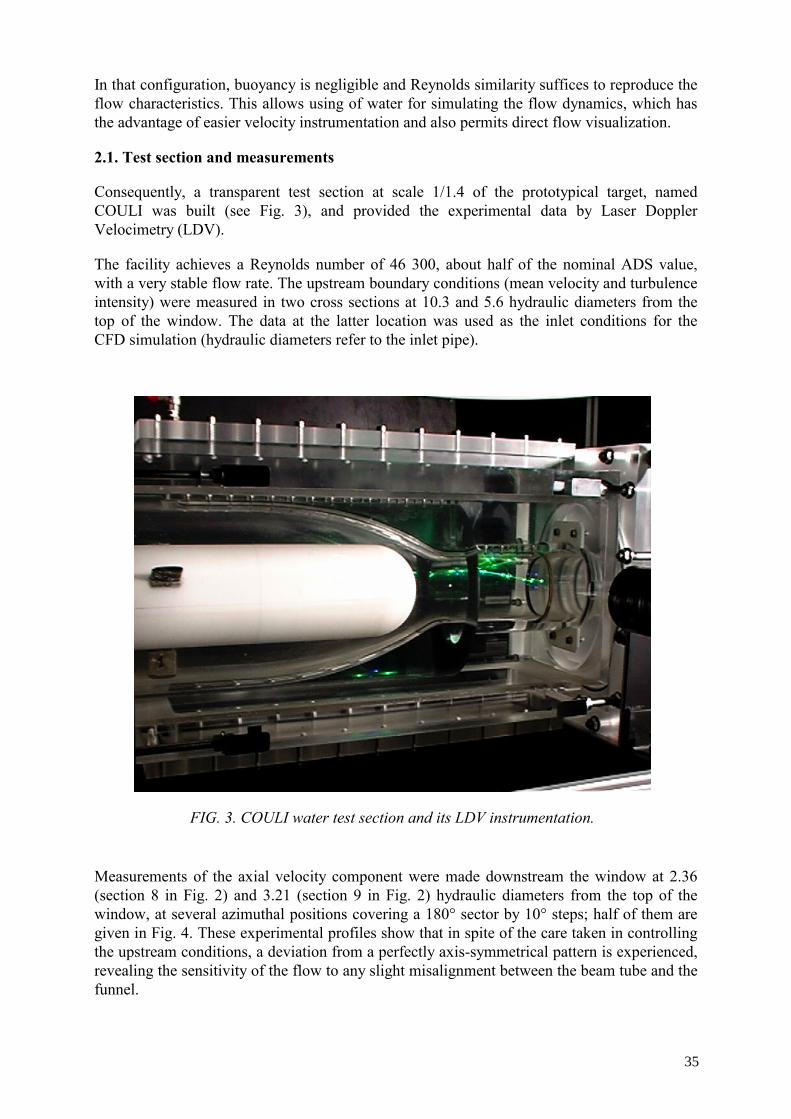
In that configuration, buoyancy is negligible and Reynolds similarity suffices to reproduce the flow characteristics. This allows using of water for simulating the flow dynamics, which has the advantage of easier velocity instrumentation and also permits direct flow visualization.

2.1. Test section and measurements

Consequently, a transparent test section at scale 1/1.4 of the prototypical target, named COULI was built (see Fig. 3), and provided the experimental data by Laser Doppler Velocimetry (LDV).

The facility achieves a Reynolds number of 46 300, about half of the nominal ADS value, with a very stable flow rate. The upstream boundary conditions (mean velocity and turbulence intensity) were measured in two cross sections at 10.3 and 5.6 hydraulic diameters from the top of the window. The data at the latter location was used as the inlet conditions for the CFD simulation (hydraulic diameters refer to the inlet pipe).

FIG. 3. COULI water test section and its LDV instrumentation.

Measurements of the axial velocity component were made downstream the window at 2.36 (section 8 in Fig. 2) and 3.21 (section 9 in Fig. 2) hydraulic diameters from the top of the window, at several azimuthal positions covering a 180° sector by 10° steps; half of them are given in Fig. 4. These experimental profiles show that in spite of the care taken in controlling the upstream conditions, a deviation from a perfectly axis-symmetrical pattern is experienced, revealing the sensitivity of the flow to any slight misalignment between the beam tube and the funnel.

35

a)

b)

FIG. 4a,b. Experimental profiles in sections 8 and 9.

More important, the region with negative values near the outer wall proves that the boundary layer detaches in the divergent, which is also evidenced by flow visualization.

36

2.2. CFD simulation

The main characteristics of the CFD model, built with the commercial software Star-CD® 3.10 B are given hereunder:

─ The two-dimensional flow domain extends from 5.6 hydraulic diameters upstream the window to 10 downstream.

─ In the outlet, the pressure is set constant; in the inlet, the values for the axial (streamwise) velocity component V, turbulent kinetic energy k and its dissipation ε were derived from the profiles measured on the test section, assuming a turbulent length scale of one tenth of the hydraulic diameter; other velocity components are zero.

─ Physical properties of water are constant and taken at 30°C, as in all experiments. ─ Several variants of the (k,ε) model were tested, linear and non-linear, with wall functions

for coarse grid cases or with a no slip condition applied at the wall when a low Reynolds number treatment was applied.

─ Hexahedral grid sizes varied from 4 331 cells for the coarsest resolution with wall functions to 20 206 cells for the finest one with the low Reynolds number treatment of the wall region.

─ All runs used the Quick convective scheme and were steady states solved with the SIMPLE algorithm in double precision. The convergence criterion on the residual error, set to 10-4, was always reached.

Regarding the effects of the grid or of the modelling at the wall boundary, no significant sensitivity was observed, but the most striking result of the computations was that the predictions of all different cases collapsed into two families:

(1) All computations using the quadratic-non linear-version of the (k,ε) model predicted a boundary layer detachment on the outer wall of the diverging section, as can be seen in Fig. 5. The associated recirculation extends on about 1.7 hydraulic diameter on the downstream two thirds of the concave outer wall.

(2) Contrarily, the standard linear form of the (k,ε) model did not show any significant detachment, whatever the resolution used to describe the boundary layer.

FIG. 5. Velocity vectors plot in the target funnel.

37

For comparison with the computations, an azimuthal average of the experimental profiles measured in the two sections downstream the window was made and then renormalized to match the flow rate.

Figure 6 makes it clear that the standard (k,ε) model is unable to predict the boundary layer detachment on the flow guide wall.

FIG. 6. Comparison of CFD prediction with experiment.

In spite of the experimental azimuthal discrepancy and although it overestimates the velocity close to the inner wall, the quadratic model prediction is close to the average flow behaviour.

Consequently when computing the flow in an ADS target whose streamlining is intended to avoid any steady boundary layer detachment, it is compulsory to use an advanced form of the (k,ε) model, as the standard version would ignore the problem.

3. MEGAPIE TARGET

3.1. General

The megawatt pilot experiment (MEGAPIE) is a lead-bismuth cooled target under construction that will be installed in the SINQ facility of the Paul Scherrer Institute in Switzerland (see Fig. 7).

In this second application, the flexibility of CFD is used to optimise the flow in the U-turn “active” region at the bottom of the target by modifying the geometry of some internal structures, especially the nozzle at the end of the by-pass tube.

38

FIG. 7. View of a 180° sector of MEGAPIE bottom end showing internal structures.

FIG. 8. Eight nozzle geometrical parameters.

δ

α

90°

H+

nozzle

by-pass tube

hull

instrumentation rod

flow guide (riser)

hemispherical window

COLD INFLOW IN ANNULAR DOWNCOMER

HEATED ZONE

HOT OUTFLOW IN RISER

39

In a perfectly axisymmetrical U-turn geometry, it is well known that a stagnation region would exist at the centre of the hemisphere, with poor cooling performance. In MEGAPIE, several arrangements were designed to promote a transverse flow on the hemispherical wall to achieve its effective cooling: the bottom edge of the flow guide tube is not horizontal but slanted and an auxiliary branch directs a cold by-pass flow on the heated wall.

Consequently, the role of several design parameters that influence the temperature and strength of this transverse flow has to be assessed; such parameters are:

─ The temperature distribution at the top of the downcomer and of the by-pass tube;

─ The heat transfer through the guide tube between riser and downcomer;

─ The value of the slant angle of the guide tube;

─ The amount of by-passed flow;

─ The shape, position and orientation of the nozzle outlet cross-section.

As it focuses on the window cooling, the present study deals with the last three items and assumes some modelling simplifications described in the next section.

3.2. Main modelling characteristics

─ Geometry: the half sector model extends up to 486 mm above the window inner face centre (model datum); the guide tube is slanted and the nozzle installed on the large gap side;

─ Structures: the central instrumentation rod is not modelled an the flow guide tube and by-pass tubes are represented by “baffles” (zero thickness elements); of course 3D conduction is accounted for in the window hemisphere;

─ Material physical properties depend on temperature for the HLM but do not for the solid;

─ Turbulence is accounted for with the standard linear (k,ε) model and the turbulent Prandtl number is 0.9;

─ Boundary conditions are:

(i) Uniform pressure at the riser outlet;

(ii) Total inlet flow rate 40 kg/s, 1.0 to 3.5 kg/s being bypassed;

(iii) Turbulence intensity 1% and turbulent length scale 2 mm at inlets;

(iv) Standard wall functions for dynamic quantities at structure walls;

(v) Norris&Reynolds two layer treatment at the window wall only;

(vi) Adiabatic outer surfaces and internal structures;

(vii) Temperatures at model inlets are extracted from full height computations that account for the heat transfer through all structures, such computations yield (see Tables 1 and 2).

─ Heat source distribution yields a power deposition is about 710 kW in the HLM and 5 400 W in the window; there is no heat source in internal structures. Note that the beam horizontal cross section is not circular but elliptical.

40

TABLE 1. DOWNCOMER TEMPERATURES

Radius (mm) 61.7 65.0 70.0 80.0 88.0

T downcomer (°C) 325 288 268 251 244

TABLE 2. NOZZLE TEMPERATURE AS FUNCTION OF BY-PASS FLOW

By-pass flow (kg/s) 1.0 1.75 2.5 3.5

T nozzle (°C) 251 246 243 240

3.3. Design parameters

The effect of the following parameters was examined:

─ By-pass flow rate of 1, 1.75, 2.5, and 3.5 kg/s;

─ Slant angle corresponding to a 25/12 mm or 30/10 mm max/min vertical gaps between the flow guide lower edge and the window inner wall;

─ Beam footprint orientation perpendicular or parallel to slant direction;

─ Nozzle angle along the window curvature α = 0, 30, or 40°;

─ Nozzle distance to the window wall δ = 2.5 or 5 mm

─ Shape of the nozzle outlet according to the Table 3.

TABLE 3. NOZZLE OUTLET SHAPES

Shape Height, mm

Width, mm

Aspect ratio

“Flat” ellipse 10 25.4 2.54

Rectangular 10 21.0 2.10

“Round” ellipse 13 19.5 1.50

The only geometrical requirement put on the nozzle is to have a “reference” cross section of 200 mm2. The reference nozzle position is α = 30° and δ = 2.5 mm.

It must be noted that for two configurations, the “round” nozzle and the “offset” rectangular nozzle (δ = 5mm), the nominal 25/15mm flow guide slant had to be increased to 30/10 mm otherwise these nozzles do not fit into the vertical gap between flow guide and window. The

41

so-called “vertical” nozzle, corresponding to α = 0°, is simply the same as the rectangular nozzle without the curved final section, it then ends 67 mm above the datum.

3.4. CFD Results

The results presented in this section were obtained with Star-CD® 3.15 steady states runs solved with the SIMPLE algorithm.

They led to stable and converged solutions (residuals less than 10-3). The total heat balance on the whole domain was of a few Watts.

The y+ range on the walls globally complied with the requirements of the boundary layer treatment employed.

3.5. Effect of the flow guide slant angle

Increasing the slant so that the vertical gap at the lower edge becomes 30/10 mm increases the pressure loss in the U-turn by about 10% and has a moderate effect on the velocity field, as seen in Fig. 10 that shows velocity vector plots in a cross section at the symmetry plane and in a layer of fluid at the window inner wall.

Consequently the gain on the window maximum temperature is only 3°C. Nevertheless the extra 5 mm provided on the larger gap side leave more flexibility to draw the nozzle shape if needed, so that the higher slant guide tube is a viable alternative to the reference 25/15 mm value.

FIG. 9. Effect of the guide tube slant in the U-turn region.

42

3.6. Effect of the flow split

Varying the bypass flow rate results in more or less efficiently sweeping the window wall, the higher its value the better the cooling but the stronger the backflow into the downcomer on the side opposite the nozzle (see Fig. 10).

FIG. 10. Effect of the by-pass flow rate on the window temperatures (nozzle jet sweeps from left to right).

3.7. Effect of the beam footprint orientation

Because buoyancy has no incidence in this type of flow, the velocity field is not affected, but as can be expected from a longer residence time of the HLM inside the spallation zone, an elliptical beam footprint oriented parallel to the jet yields higher temperatures and steeper gradients in the symmetry plane of the window.

The increase varies from 7 to 21°C depending on the type of nozzle tested (see Fig. 11).

Wall jet direction

43

FIG. 11. Effect of the orientation of the beam footprint on the window temperatures with a rectangular nozzle.

3.8. Effect of the nozzle geometry

Depending on how the nozzle jet interacts with the downcomer flow, impinges and spreads on the window concave wall, various temperature patterns are obtained, with the hottest spots either on the symmetry plane or aside of it.

Figure 12 shows the various temperature maps obtained on the window outer wall, its temperature scale ranges from 240 to 380°C by 10°C steps.

Temperature distributions for various nozzle types are given in Table 4. Temperature profiles along two perpendicular meridians of the window, one in plane [OXZ] and one in plane [OYZ], are shown in Fig. 13.

Wall jet direction

44

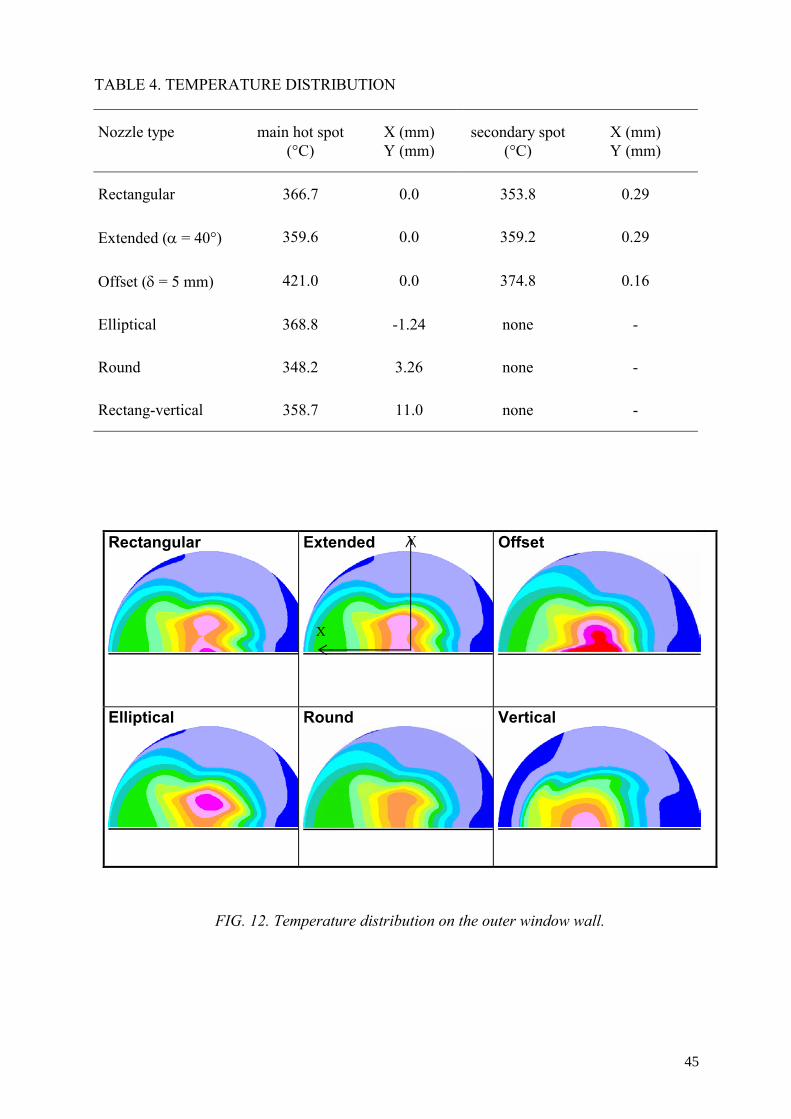
TABLE 4. TEMPERATURE DISTRIBUTION

Nozzle type main hot spot (°C)

X (mm) Y (mm)

secondary spot (°C)

X (mm) Y (mm)

Rectangular 366.7 0.0 353.8 0.29

Extended (α = 40°) 359.6 0.0 359.2 0.29

Offset (δ = 5 mm) 421.0 0.0 374.8 0.16

Elliptical 368.8 -1.24 none -

Round 348.2 3.26 none -

Rectang-vertical 358.7 11.0 none -

Rectangular Extended Offset

Elliptical Round Vertical

FIG. 12. Temperature distribution on the outer window wall.

Y

X

45

a)

b)

FIG. 13a,b. Temperature profiles along window curvature.

46

Principal observations are summarized as:

─ Maximum temperatures are in the 350 to 370°C range, except in the offset position where 420°C are reached, showing sensitivity to the parameter δ;

─ The best performance in terms of maximum window temperature is obtained with the elliptical nozzle of low aspect ratio (referred to as “round”) installed with the 30/10 mm slanted flow guide;

─ The vertical rectangular nozzle comes second, closely followed by the extended rectangular nozzle;

─ Temperature gradients parallel to the window surface remain under 6 000°C/m.

4. CONCLUSION

Depending on their ultimate use, HLM cooled spallation targets equipped with a solid window fall into two main types of designs. Because of the extreme conditions of heating and irradiation exerted on the containing structure, each type requires an accurate prediction of the flow pattern and its corresponding cooling performance, which primarily depends on the specific capabilities of the turbulence modelling.

Concerning ADS targets, the capability of the model to predict boundary layer detachment is at stake, as no optimisation of the funnel streamlining can be expected from models that would not catch this aspect. To that respect some model predictions were compared against the experimental data obtained on a water model operating at a representative Reynolds number. It was concluded that only non standard, but advanced forms of the (k,ε) model were needed to predict correctly the flow pattern.

Concerning targets where the flow in the active zone is in a U-turn configuration and sweeps the concave side of the window, testing the merits of various turbulence models is still undergoing and requiring to be compared with experiments before similar conclusions are drawn. Nevertheless CFD has proven a flexible and invaluable tool to investigate the comparatively more complex flow pattern and the numerous associated design parameters, therefore contributing to bring useful information for orienting the design of a HLM target, as was illustrated by the example of MEGAPIE.

47

CFD ANALYSIS OF THE THERMAL-HYDRAULIC PERFORMANCE OF THE ESS TARGET

E.M.J. KOMEN, F. ROELOFS Nuclear Research and Consultancy Group (NRG), Petten, Netherlands

J. WOLTERS, G. HANSEN Forschungszentrum Jülich (FZJ), Jülich, Germany A.1.1. Abstract

This paper presents the Computational Fluid Dynamics (CFD) analyses performed in order to determine the effects of the mass flow distribution within the target of the European Spallation Source on the window and the liquid mercury temperature. For flow distributions where less than about 23% of the total mass flow rate flows through the bottom ducts, the CFD analyses show that the: ─ Computed maximum window temperatures are 115 to 90 K below the maximum allowable temperature of

673 K for a 1.5 mm thick window; ─ Computed maximum liquid mercury temperatures are 5 to 30 K below the maximum allowable temperature

of 573 K; ─ Flow distribution where about 15% of the total mass flow rate passes through the bottom ducts yields the

optimal temperature distribution within the target. In addition, the effect of the diameter of the injected helium bubbles on the bubble trajectories has been determined. The CFD analyses show that 0.5, 0.25, and 0.1 mm diameter helium bubbles will accumulate in flow re-circulation zones that are present in the window region. However, in the CFD simulations, helium bubbles smaller than 0.05 mm do not accumulate in these re-circulation zones.

1. INTRODUCTION

The European Spallation Source (ESS) is based on the coupling of a linear accelerator with a liquid mercury spallation target. This linear accelerator generates a proton beam that penetrates into the so-called window region of the spallation target. Inside the target, accelerated protons react with mercury nuclei through a spallation reaction. Thereby, the desired fast neutrons are created. During the spallation process, the proton beam causes a pulsed heat deposition inside the liquid mercury. This pulsed heat deposition causes a pressure wave inside the target [10]. This pressure wave may violate the structural integrity of the target. A possible solution to mitigate the pressure wave is to inject small helium bubbles in the liquid mercury, thereby introducing compressibility in this flow.

Within the European Spallation Source (ESS) project, Forschungszentrum Jülich (FZJ, Germany) is responsible for the design of the spallation target. In a bilateral co-operation with FZJ, the Nuclear Research and Consultancy Group NRG (The Netherlands) performs Computational Fluid Dynamics (CFD) analyses [4–7, 11] in order to support FZJ with this. The objective of these CFD analyses is to determine suitable flow distributions and helium bubble diameters fulfilling the following three requirements [16]:

─ The window temperature should stay below 673 K; ─ The local liquid mercury temperatures within the target should stay below 573 K (a safety

margin of 50 K with respect to the evaporation temperature at 1 bar was stated, that will even increase for higher mercury pressure);

─ Accumulation of helium bubbles within the target should be avoided.

For this purpose, the window temperature, the liquid mercury temperature field, and the bubble trajectories during steady state time-averaged heat deposition were determined as a function of the

49

mass flow rate distribution inside the ESS target design using CFD. This mass flow rate distribution inside the target can be controlled using orifices in the inlet ducts of the target. This is the MS-Word template for preparing full-length manuscripts for review and final manuscript after review. Please follow the instructions as closely as possible.

2. CFD MODEL

2.1. Computer codes

The computations have been performed using the widely used commercial CFD codes STAR-CD 3.15 [23] and CFX-4.4 [2]. In Ref. [7], it is demonstrated that the differences between the STAR-CD 3.15 and CFX-4.4 results can be practically neglected for the current application when the same turbulence model and the same numerical settings are used. The results obtained using STAR-CD 3.15 are presented in this paper.

2.2. Mesh

The mesh for the complete model is presented in Fig. 1. This mesh consists of 1 860 000 hexahedral computational cells. In the current computations, symmetry has been used. As a result, half of the complete model could be used (930 000 computational cells). The mesh size sensitivity analysis performed in [11] indicates that the applied mesh is sufficiently fine. That is, the numerical errors resulting from the spatial discretization can be practically neglected.

The low Reynolds number k-ε turbulence model of [9] as implemented in STAR CD 3.15 has been selected for the current analyses. Therefore, the mesh has been refined near the walls in the window region such that the non-dimensional distance y+ is smaller than 1 in order to resolve the boundary layers.

FIG. 1. Mesh of the ESS liquid mercury target (1 860 000 hexahedral computational cells).

Inlet Manifold

Oultlet Manifold

Target Window

50

Concerning the modelling of the solid structures, the window wall is included in the current model. The presence of internal structures is taken into account. Figure 2 shows an internal view in the ESS model.

FIG. 2. View inside the ESS geometrical model. The window has been cut from the ESS target model.

The modelling of conduction through the internal structures is envisaged as a next step in the extension of the current model.

2.3. Main fluid dynamics model

The main fluid dynamics model describes a steady state time-averaged incompressible turbulent flow including heat transport and buoyancy. For computation of the trajectories of the helium bubbles, the Eulerian-Lagrangian two-phase flow modelling approach has been applied.

For the present application, the drag force due to the bubbles is negligible compared to the momentum flux of the liquid metal. Therefore, one-way momentum coupling between the two phases has been used in the applied Eulerian-Lagrangian two-phase flow model. That is, the influence of the presence of the bubbles on the continuous phase momentum transport is neglected.

Because the bubble volume fraction is smaller than 1%, bubble-bubble interaction (bubble-bubble collision, coalescence, or break-up) has been neglected. A perfect rebound model has been applied in order to model bubble-wall interaction.

51

2.4. Physical properties

For the density, conductivity, specific heat, and dynamic viscosity of liquid mercury, temperature dependent values have been used over the temperature range of 273 to 623 K, as obtained from [3]. For the steel window wall, the temperature dependent thermal conductivity of steel 1.4922 as obtained from [12] has been used, whereas constant values are used for the density and specific heat.

2.5. Boundary conditions

The inlet boundary conditions as used at the inlet of the computational domain, i.e. the inlet manifold, are specified in Table 1.

TABLE 1. INLET BOUNDARY CONDITIONS

Quantity Value

Velocity, m/s 1.0524

Temperature, K 373

Turbulence intensity, K 4

Turbulence length scale, M 0.0125

At the outlet of the computational domain, a static pressure of 0.1 MPa is used, whereas zero normal gradients are used for all remaining flow variables, corresponding to fully developed flow variables. The outer window wall is assumed to be adiabatic.

2.6. Heat deposition

The proton beam results in a pulsed heat deposition in the window wall and the liquid mercury coolant flow. However, a steady state heat deposition has been used as a first step in order to circumvent CPU-time consuming time-dependent analyses. Therefore, the pulsed heat deposition profile has been converted to a time averaged heat deposition profile. This time averaged heat deposition profile has been obtained from [14]. Using this heat deposition profile, a total thermal power of 9.1 kW is generated in the target window, whereas 2.9 MW is generated in the liquid mercury.

2.7. CFD Model validation

2.7.1. Turbulent momentum transport modelling

For turbulent momentum transport, the capabilities and limitations of k-ε based turbulence models for Heavy Liquid Metal (HLM) flows are comparable to those of common fluids. These capabilities and limitations are quite well known. However, in order to quantify the accuracy of the modelling of the turbulent momentum transport for ESS, FZJ will perform experiments in a full scale water loop model. Therefore, this accuracy will be quantified in the near future, following the availability of the experimental data.

52

2.7.2. Near wall heat transfer modelling

Concerning near wall heat transfer modelling, the major issue is that HLM’s are fluids with a very low Prandtl number compared to standard fluids (e.g. water). As a result, the thermal boundary layer thickness in HLM flows is much larger than the velocity boundary layer thickness.

For validation of the near wall heat transfer modelling, experimental correlations [1, 15] and experimental data from the ESS-HETSS experiment have been used. This experiment has been used as a benchmark within the ASCHLIM project (ASsessment of Computational fluid dynamics codes for Heavy Liquid Metals, EU 5th framework project) [17]. From the validation results presented in Refs [6, 17], it could be concluded that 2-equation low Reynolds number k-ε turbulence models as used in the present paper can compute the heat transfer coefficient for the ESS window cooling with engineering accuracy (typically within 30%) provided that the flow remains attached to the window wall.

2.7.3. Modelling of turbulent heat transport within the bulk

For the turbulent heat transport within the bulk of HLM flows, the major modelling issue is related to the application of a constant turbulent Prandtl number in the model for the turbulent mixing in 2-equation k-ε turbulence models. From the ESS-HETSS experiment which has been used as a benchmark within the ASCHLIM project, it could be concluded [17] that the default constant turbulent Prandtl number of 0.9 can be used for high Reynolds number flows of HLM’s, i.e., low Prandtl number fluids (Re > O(106); Pe > O(104)). More arguments for this conclusion are given in [8].

2.7.4. Modelling of helium bubble transport

Currently, there is no measuring technique available providing reliable information about the bubble shape and the bubble trajectories in HLM two-phase flows. As a result, there is no experimental database available for HLM two-phase flows. Therefore, it has not been possible to validate the applied Eulerian-Lagrangian two-phase flow model for the current purposes. However, in order to reach a certain level of verification/validation, the following two cases have been considered in [4]:

─ Mercury “bubble” in a liquid mercury solid body rotation (verification case); ─ Terminal rise velocity of spherical air bubbles in water (validation case).

Based on the results obtained for these cases, it could be concluded that:

─ The implementation of the steady state drag force, the pressure gradient force, and the gravitational body force in the applied two-phase flow model is correct;

─ The numerical results obtained for the terminal rise velocity of spherical air bubbles in water were in good agreement with the experimental result.

Based on the current status of the validation of the applied two-phase flow model, it can be concluded that only qualitative trends can be obtained for the computed bubbles trajectory.

3. RESULTS

The computed maximum window and liquid mercury temperatures are presented graphically in Fig. 3. As can be seen in this figure, the window temperatures have been computed for a 1.5 and 3.0 mm thick window. The allowable maximum window temperature of 673 K and the allowable maximum liquid mercury temperature of 573 K are also presented in Fig. 3. The maximum liquid mercury

53

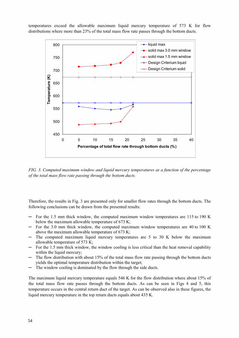
temperatures exceed the allowable maximum liquid mercury temperature of 573 K for flow distributions where more than 23% of the total mass flow rate passes through the bottom ducts.

FIG. 3. Computed maximum window and liquid mercury temperatures as a function of the percentage of the total mass flow rate passing through the bottom ducts.

Therefore, the results in Fig. 3 are presented only for smaller flow rates through the bottom ducts. The following conclusions can be drawn from the presented results:

─ For the 1.5 mm thick window, the computed maximum window temperatures are 115 to 190 K below the maximum allowable temperature of 673 K;

─ For the 3.0 mm thick window, the computed maximum window temperatures are 40 to 100 K above the maximum allowable temperature of 673 K;

─ The computed maximum liquid mercury temperatures are 5 to 30 K below the maximum allowable temperature of 573 K;

─ For the 1.5 mm thick window, the window cooling is less critical than the heat removal capability within the liquid mercury;

─ The flow distribution with about 15% of the total mass flow rate passing through the bottom ducts yields the optimal temperature distribution within the target;

─ The window cooling is dominated by the flow through the side ducts.

The maximum liquid mercury temperature equals 546 K for the flow distribution where about 15% of the total mass flow rate passes through the bottom ducts. As can be seen in Figs 4 and 5, this temperature occurs in the central return duct of the target. As can be observed also in these figures, the liquid mercury temperature in the top return ducts equals about 435 K.

450

500

550

600

650

700

750

800

0 5 10 15 20 25 30 35 40

Percentage of total flow rate through bottom ducts (%)

Tem

pera

ture

(K)

liquid maxsolid max 3.0 mm windowsolid max 1.5 mm windowDesign Criterium liquidDesign Criterium solid

54

FIG. 4. Computed liquid mercury temperature field in the horizontal mid-plane of the target for the flow distribution where 15% of the total mass flow rate flows through the bottom ducts.

FIG. 5. Computed liquid mercury temperature field in the horizontal mid-plane of the target for the flow distribution where 15% of the total mass flow rate flows through the bottom ducts.

The maximum liquid mercury temperature will be lower for the situation where the liquid mercury temperature in the top return ducts is equal to the liquid mercury temperature in the central return duct. Therefore, it is recommended to investigate partial blockage of the top return ducts in order to:

─ Reduce the mass flow rate through these top return ducts; ─ Increase the mass flow rate through the central return duct.

55

This way, a more homogeneous temperature field within the return ducts of the target is obtained, resulting in a lower maximum liquid mercury temperature.

FIG. 6. Liquid mercury flow paths in the ESS target.

The liquid mercury flow paths in the target are presented in Fig. 6. For the flow distributions analysed in this paper, the major part of the total mass flow rate flows through the side ducts. Due to this mass flow rate distribution, two re-circulation zones appear in the window region. Low static pressures occur in the core of these re-circulation zones. These low pressures result in a strong pressure gradient force acting on the helium bubbles. For bubble diameters of 0.5, 0.25, and 0.1 mm, this pressure gradient force drives almost all bubbles to the core of the two re-circulation zones. As a result, accumulation of almost all injected helium bubbles takes place in the window region (see Fig. 7). However, for sufficiently small bubbles (i.e. bubble diameter smaller that 0.05 mm in the CFD simulations), the drag force dominates the pressure gradient force. As a result, these small bubbles do not accumulate anymore in the re-circulation zones.

4. CONCLUSIONS

For total percentage bottom duct flows smaller than about 23%, the following conclusions have been drawn from the presented results:

─ For the 1.5 mm thick window, the computed maximum window temperatures are 115 to 90 K below the maximum allowable temperature of 673 K;

─ For the 3.0 mm thick window, the computed maximum window temperatures are 40 to 100 K above the maximum allowable temperature of 673 K;

─ The computed maximum liquid mercury temperatures are 5 to 30 K below the maximum allowable temperature of 573 K;

─ For the 1.5 mm thick window, the window cooling is less critical than the heat removal capability within the liquid mercury;

56

─ The flow distribution with about 15% of the total mass flow rate passing through the bottom ducts yields the optimal temperature distribution within the target.

─ The estimated error in the computed maximum window temperatures equals 20 K; ─ 0.5, 0.25, and 0.1 mm diameter helium bubbles accumulate in the re-circulation zones in the

window region; ─ Sufficiently small helium bubbles (i.e., bubble diameter smaller that 0.05 mm in the

CFD simulations) do not accumulate in these re-circulation zones. Coalescence of helium bubbles has not been analysed, but remains a subject for future analyses.

FIG. 7. Computed trajectories of 0.1 mm diameter helium bubbles. The helium bubbles are injected via the bottom inlet ducts.

REFERENCES

[1] BUCENIEKS, I., et al., ESS Mercury Target Model Experiments: Investigations on

the Heat Transfer, ESS 98-73-T, University of Latvia, Latvia (1998). [2] CFX 4.4 USER GUIDE, Computational Fluid Dynamics Services, AEA Technology,

Harwell laboratory, Oxfordshire OX11 0RA, United Kingdom (2001). [3] CORDS, H., A Literature Survey on Fluid Flow Data for Mercury – Constitutive

Equation-. ESS 98-81-T, Forschungszentrum Jülich GmbH, Germany (1998). [4] KOMEN, E.M.J., KONING, H., CFD Analysis of Helium Bubble Flow in the ESS

Target; initial Target Design without Orifices, NRG report 20619/01.39634/C, Petten, Netherlands (November 2001).

[5] KOMEN, E.M.J., KONING, H., CFD Analysis of Helium Bubble Flow in the ESS Target; Initial Target Design with Orifices. NRG report 20619/01.43740/C, Petten, Netherlands (December 2001).

[6] KOMEN, E.M.J., KONING, H., Determination of Flow Distributions with sufficient Heat Removal Capability within the ESS target; Reference Target Design with Orifices, NRG report 20619/01.43740/C, Petten, Netherlands (December 2001).

57

[7] KOMEN, E.M.J., KONING, H., Determination of suitable Flow Modes for operating the ESS Target; Initial Target Design with Orifices, NRG report 20913/02.47144/C, Petten, Netherlands (June 2002).

[8] KOMEN, E.M.J., KONING, H., ROELOFS, F., Determination of Flow Distributions with sufficient Heat Removal Capability within the ESS Target, NRG report 20913/02.50134/C, Petten, Netherlands (March 2003).

[9] LIEN, F.S., CHEN, W.L., LESCHZINER, M., Low Reynolds Number Eddy Viscosity Modelling based on non-linear Stress-Strain/Vorticity Relation, Proc. 3rd Symp. Engineering Turbulence Modelling and Measurements, Crete, Greece, 27–29 May 1996, Elsevier Science, ISBN 0444824634 (1996).

[10] PROBST, U., Numerical calculation on pressure pulses in the mercury tank of the ESS spallation target and aspects concerning its optimization, ESS 01-117-T, Forschungszentrum Jülich (2001).

[11] ROELOFS, F., et al., CFD Analyses on the ESS Mercury Target Unit; Single-phase, isothermal, incompressible flow, NRG report 20289/00.33125/C, Petten, Netherlands (June 2000).

[12] STAHL-EISEN-WERKSTOFFBLÄTTER DES VEREINS DEUTSCHER EISENHÜTTENLEUTE, SEW 310 – Physikalische Eigenschaften von Stählen (August 1992).

[13] STAR-CD 3.15 USER GUIDE, Computational Dynamics Limited, 200 Shephers Buch Road, London, W6 7NY, U.K. (2001).

[14] THE EUROPEAN SPALLATION SOURCE, Vol. III - The Technical Study, ESS Report 96-53-M, ISBN 090 237 6500 (November 1996).

[15] WHITE, F.M., Viscous Fluid Flow, McGraw-Hill Inc., second edition, York (1991). [16] WOLTERS, J., Preparations for Meeting 7-2-2002, E-mail from FZJ to NRG

(January 2002). [17] WOLTERS, J., (Ed.) ESS-HETSS Computational Benchmark Summary Report

Forschungszentrum Jülich GmbH, Germany (2003).

58

VALIDATION OF CFD MODELS WITH RESPECT TO THE THERMAL-HYDRAULIC DESIGN OF THE ESS TARGET

J. WOLTERS, G. HANSEN Forschungszentrum Jülich GmbH (FZJ), Jülich, Germany

E.M.J. KOMEN, F. ROELOFS Nuclear Research and Consultancy Group (NRG), Petten, Netherlands

Abstract

For the proposed next generation neutron source for Europe ESS (European Spallation Neutron Source), the thermal-hydraulic design of the target is one of the main issues. The design will concentrate on the heat removal capability of the target, flow stability, and active cooling of the target window by the mercury flow. Moreover the behaviour of gas bubbles, which will be necessary to mitigate the pressure pulse inside the target, will be considered in the thermal-hydraulic design. Because Computational Fluid Dynamics (CFD) is one of the main tools to be used for the thermal-hydraulic design, validation of corresponding models in available CFD codes is a very important matter within the ESS project. Up to now, a lot of validation work took place within the European Commission funded ASCHLIM project. From the analyses performed within this project and additional validation work performed by NRG and FZJ, it could be concluded, that CFD codes are in principal able to predict the wall cooling at the target window with engineering accuracy if certain ancillary conditions are considered. In order to quantify the accuracy of the RANS modelling of the turbulent momentum transport for the ESS target concept, an experiment with a prototype target, made of acrylic glass, in a water loop was set up. Velocity field measurements, using Particle Image Velocimetry (PIV), will be performed, and the measured flow field will be compared to CFD results. With respect to the transport of small gas bubbles in a mercury flow, up to now no suitable experiments are available for the validation work needed for the ESS target, and therefore, only some basic investigations took place.

1. INTRODUCTION

The European Spallation Neutron Source (ESS) is the proposed next generation neutron source for Europe. Two target stations were foreseen for ESS (long pulsed and short pulsed), with a time averaged proton beam power of 5 MW for each target. Mercury was chosen to be the target material, because of its favourable properties with regard to heat transfer and nucleonics. Forschungszentrum Jülich (FZJ, Germany) is responsible for the design of the targets. In a bilateral co operation with FZJ, the Nuclear Research and Consultancy Group NRG (Netherlands) supports FZJ regarding the thermal-hydraulic design of the target.

For the thermal-hydraulic design of the target and safety analyses, Computational Fluid Dynamics (CFD) is one of the main tools to be used. Investigations will concentrate on the heat removal capability of the target, flow stability, and active cooling of the target window by the mercury flow. In case helium bubbles will be used in the ESS target to mitigate the generated pressure pulses inside the liquid mercury, bubble transport will also be considered in the thermal-hydraulic design. Validation of corresponding CFD models is a main task within the project. This paper will summarize the validation work that has been done with respect to the thermal-hydraulic design of the ESS target.

2. VALIDATION WORK IN THE FIELD OF TURBULENT MOMENTUM TRANSPORT

In the RANS CFD approach, the Reynolds Averaged Navier Stokes (RANS) equations are solved. This way, time-averaged flow variables are obtained. Standard 2-equation RANS turbulence models have been validated for Heavy Liquid Metal (HLM) flows within the EU 5th framework ASCHLIM project (ASsessment of Computational fluid dynamics codes for Heavy Liquid Metals) [1]. It can be concluded, that the capabilities and limitations of standard RANS turbulence models for turbulent momentum transport in HLM flows are

59

comparable to those of common fluids. To quantify the accuracy of the RANS modelling of the turbulent momentum transport for the ESS target, experiments in a water loop model are sufficient. In Fig. 1a (left hand side) the corresponding plexiglass target, which was set up in a water loop at the central department of technology in FZJ, is shown. The flow field measurements are done using Particle Image Velocimetry (PIV). The velocity distribution in the plane spanned by the laser (see Fig. 1b, for a horizontal plane) is determined by photographically recording the motion of microscopic particles that follow the fluid flow.

1a) 1b)

FIG. 1. Flow measurement in the ESS plexiglass target using Particle Image Velocimetry (PIV).

The work in this field is still going on, and an assessment of results on the corresponding benchmark calculations in comparison to the experimental results are not available jet.

2.1. ESS mercury target model experiment

To gain the basic understanding on the heat transfer at the beam window of the ESS target, basic investigations were performed on a test section in a mercury loop, which was build up at the Institute of Physics at the University of Latvia. A detailed description of the experimental set up of the so-called ‘ESS mercury target model experiment’ or simply ‘ESS HETSS experiment’ is given in Ref. [2]. A sketch of the test section is given in Fig. 2 showing the distribution of Heat Emitting and Temperature Sensing Surfaces (HETSS) along the surfaces of the active part of the channel. The measuring principle of the HETSS is described in detail in Ref. [2].

60

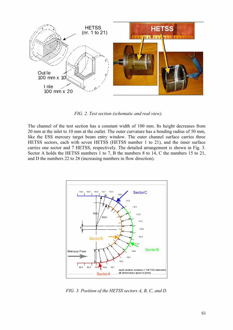
HETSS (nr. 1 to

Outle100 mm x 10

Inle100 mm x 20

HETSS (nr. 1 to 21)

Outle100 mm x 10

Inle100 mm x 20

FIG. 2. Test section (schematic and real view).

The channel of the test section has a constant width of 100 mm. Its height decreases from 20 mm at the inlet to 10 mm at the outlet. The outer curvature has a bending radius of 50 mm, like the ESS mercury target beam entry window. The outer channel surface carries three HETSS sectors, each with seven HETSS (HETSS number 1 to 21), and the inner surface carries one sector and 7 HETSS, respectively. The detailed arrangement is shown in Fig. 3. Sector A holds the HETSS numbers 1 to 7, B the numbers 8 to 14, C the numbers 15 to 21, and D the numbers 22 to 28 (increasing numbers in flow direction).

SectorD

SectorA

SectorB

SectorC

FIG. 3. Position of the HETSS sectors A, B, C, and D.

61

Figure 4 shows the test section mounted to the mercury loop.

FIG. 4. Test section mounted to the mercury loop.

Each sector could be heated separately in the experiment and different combinations of heated sectors were investigated. But the benchmark calculations were only done for the cases where all outer sector (A, B, and C) were heated with a constant heat flux of 6.9 W/cm2, because for this case experimental results are available even for higher Reynolds numbers. The mercury flow-rate is the major parameter that was varied during the sessions. A flow-rate of up to 1.5 L/s was used for the experiments.

2.2. CFD model for calculations on the ESS mercury target model experiment

The CFD model used for the calculations at FZJ and NRG is in principle shown in Fig. 5.

FIG. 5. CFD model of test section.

The fluid region of the test section, the inlet region, and the outlet region was modelled. The solid walls were not modelled explicitly, but were considered by adequate boundary conditions. Due to the symmetry regarding geometry and boundary conditions, most of the calculations were done with a half-model. For mercury, temperature dependant fluid properties according to [3] were considered.

62

2.3. Results

During the experiments only temperatures at the HETSS could be measured. There are no experimental data available for velocities or turbulence in the test section. Therefore, only calculated temperatures at the HETSS will be compared to the experiment. In order to look in detail to differences between the numerical results, a comparison of velocities, temperatures and turbulence was done for the CFD calculations [4].

2.3.1. Experimental results

The temperature increment for the HETSS with respect to the reference (inlet) temperature of 283 K is shown in Fig. 6 for different flow-rates.

0

2

4

6

8

10

12

14

16

18

1 6 11 16 21

HETSS

ΔT

[K]

.

0.1 l/s0.5 l/s1.0 l/s1.5 l/s

FIG. 6. Temperature increment along the HETSS for different volumetric flow-rates.

According to Ref. [4], the original measurement was slightly adjusted to clear small deviations due to calibration. It is obvious, that for higher flow-rates the heat transfer increases, and therefore the wall temperatures decrease significantly. For all cases, the lowest wall temperature occurs at the inlet of the test section (HETSS number 1), while the maximum wall temperature occurs close to HETSS number 6 within the bent channel. Further downstream the wall temperature decreases again.2.3.2. Numerical results CFD calculations were performed by FZJ and NRG with different CFD codes and different turbulence models. FZJ used Fluent 5.5 [5] and NRG used Star CD 3.15 [6] and CFX 4.4 [7]. Different aspects were investigated within this benchmark activity, which are described in the following sections.

2.3.2.1. Effect of flow rate

The calculations on the effect of the flow rate were performed with the standard k-ε model with a two-layer zonal approach for the near wall treatment and low Reynolds number turbulence models (low Re k-ε and low Re k-ω), respectively. With respect to the calculated temperatures, the results of the single codes and turbulence models lie within a margin of about 15% and therefore agree quite well. The agreement between calculations and

63

experiment strongly depends on the flow rate. The best agreement between calculations and experiment is achieved for a maximum flow rate of 1.5 L/s. Here, the shape of the temperature distribution along the HETSS and the absolute temperatures are predicted very well (see Fig. 7).

0

1

2

3

4

5

6

1 6 11 16 21

HETSS

ΔT [K

]

experiment

k-eps, two-layer zonal model

q = 1.5 l/s

FIG. 7. Temperature increment along the HETSS calculated with the k-ε model in fluent for a flow rate of 1.5 L/s, compared to the experimental results.

For lower flow rates the temperatures are overestimated by the CFD codes. In Fig. 8 the deviations are depicted for the standard k-ε model in Fluent for a minimum flow rate of 0.1 L/s.

0

5

10

15

20

25

1 6 11 16 21

HETSS

ΔT [K

]

Experimentk-eps, two-layer zonal model

q = 0.1 l/s

FIG. 8. Temperature increment along the HETSS calculated with the k-ε model in fluent for a flow rate of 0.1 L/s, compared to the experimental results.

64

The deviations for lower flow rates can partly be explained by the neglect of the heat transfer from the sensors to the duct walls next to the sensors [8] that is not considered in the CFD models. Furthermore, the turbulence models seem to underestimate the production of turbulence for low flow-rates [4].

Regarding the design of the ESS target, the poor agreement between experimental and numerical results for lower flow rates is not of great importance, because the Reynolds number of the mercury flow in the ESS target will even exceed the one of the mercury flow in the test section at 1.5 L/s.

2.3.2.2. Effect of near wall treatment

For high Reynolds numbers, the viscous sublayer of a boundary layer is very thin. A very fine mesh has to be used near the wall for the two-layer zonal model and the low Reynolds number turbulence models, respectively, where the near-wall behaviour is integrated down to the wall. This can be avoided by using wall functions, which rely on the existence of a linear and logarithmic region in the velocity profiles.

If wall functions are used, the non-dimensional distance of the first grid point to the wall has to be within the logarithmic region of the viscous boundary layer, i.e. y+ has to be greater than 30. The upper value for y+ depends on the Reynolds number. An upper value of 500 is recommended, but strictly, the logarithmic law of the wall should only be applied to a point whose y+ value is less than 130 [5].

Reynolds' analogy between momentum and energy transport is assumed also for the wall functions. As in the law-of-the-wall for mean velocity, the law-of-the-wall for temperature employed in FLUENT comprises the following two different laws: Linear law for the thermal conduction sublayer, where conduction is important, and a logarithmic law for the turbulent region, where effects of turbulence dominate conduction.

This analogy is questionable for low-Prandtl-number fluids (e.g. heavy liquid metal), where the thickness of the thermal sublayer is much larger than that of the momentum sublayer. With respect to the heated walls of the test section, the first grid point lying in the logarithmic region of the viscous boundary layer may lie in the linear region of the thermal boundary layer, where conduction dominates the effects of turbulent energy transport.

Detailed numerical investigations on wall functions were done with Fluent for a flow rate of 1.5 L/s. In Fluent the thermal sublayer thickness is computed by the point of intersection of the linear and logarithmic law-of-the-wall. In Fluent 5, for the logarithmic law a function is used, which is only valid for moderate to high-Prandtl-number fluids. For low-Prandtl-number fluids there is no point of intersection any more (see Fig. 9). In Fluent 6, a new function is used, which results in an intersection point with the linear law, even for low Prandtl number fluids (see Fig. 9). Considering the logarithmic law given in Fluent 6, the thermal sublayer thickness y*

T for mercury (Prandtl number 0.027) is about 260.

For the calculations with wall functions, two different grid sizes were investigated. In the case of 1.5 L/s the two grids lead to y+ values of less than 130 and less than 310, respectively, at the heated wall. This denotes, that the first grid point clearly lies within the thermal sublayer for the fine mesh, while for the coarse mesh the first grid point partly lies outside of the thermal sublayer.

65

-5

0

5

10

1 10 100 1000

y*

T*linear lawlogarithmic law (Fluent 6)T* (y*)logarithmic law (Fluent 5)

y*T = 256

FIG. 9. Thermal laws-of-the-wall for mercury (Prandtl number 0.027).

The temperature distribution along the HETTS is shown for the calculations with Fluent 5 and Fluent 6 in comparison to the experimental results in Fig. 10. For the fine mesh (y+ < 130) the numerical results agree quite well with the experimental result if Fluent 5 is used. But even in this case it is apparent, that for the second half of the bend the temperatures are slightly overestimated. For the calculations with the coarse mesh (y+ < 310) and Fluent 5, as well as for both calculations performed with Fluent 6, the agreement between the numerical and experimental results is quite poor.

0

1

2

3

4

5

6

7

8

9

1 6 11 16 2 1H ET SS

T [K

]

e xperim en t

k-eps ,wall functions, y+ < 310, Fluent 5

k-eps ,wall functions, y+ < 130, Fluent 5

k-eps ,wall functions, y+ < 310, Fluent 6

k-eps ,wall functions, y+ < 130, Fluent 6

q = 1.5 l/s

FIG. 10. Temperature distribution along the HETSS for the calculations with wall functions, compared to the experimental results, for a flow-rate of 1.5 L/s.

66

A more detailed analysis of the results has shown, that with respect to the calculated values for velocity, turbulent kinetic energy, and temperature within the computational cells, the agreement between the single calculations is quite satisfactory. The discrepancies with respect to the wall temperature, in particular for the coarse mesh, are mainly caused by the extrapolation. The calculated temperatures are shown along three paths, which start at the heated wall in the plane of symmetry and which are perpendicular to the walls at the starting point (see Fig. 11). One path named ‘Inlet’ is located in the inlet region of the test section, one is in the middle of the bent channel (named ‘Bend’), and the last one named ‘Outlet’ is in the outlet region.

0

1

2

3

4

5

6

7

0 0,5 1 1,5 2

distance to outer wall [mm]

ΔT [K

]

two-layer zonal modelOutletBendInletwall functions (coarse mesh)OutletBendInlet

extrapolatedwall temperature

fist cell

Fluent 5, q = 1.5 l/s

FIG. 11. Temperature profiles along three paths of the bent channel calculated with Fluent 5 and the coarse mesh, in comparison with the results for the two-layer zonal model.

To understand the discrepancies with respect to the extrapolated wall temperature, the extrapolation procedure was checked. It was found, that Fluent 5 used the linear law for the extrapolation in all cases, while Fluent 6 always used the logarithmic law, even if the first grid point clearly lies inside of the thermal sublayer. The problem with Fluent 6 could be fixed by using user defined functions to evaluate the wall temperature, so that similar results were achieved with Fluent 5 and Fluent 6 for the first grid point lying within the thermal sublayer. The following investigations will therefore concentrate on the deviations for Fluent 5.

For the considered test section at a flow rate of 1.5 L/s, the extrapolation based on the linear law should be correct for almost all regions of the heated wall if a thermal sublayer thickness of y*

T = 256 according to Fig. 9 is considered. But the deviations in the outlet region for the calculations with the fine mesh denote, that the near wall region, where conduction dominates turbulent effects, must be much smaller than assumed by the thermal wall functions shown in Fig. 9. This leads to the conclusion, that probably a smaller value for y*

T is appropriate. To verify this, the results achieved with the two-layer zonal model were used to derive a new wall function T*(y*). The new wall function for a flow rate of 1.5 L/s is shown in Fig. 12, in

67

comparison to the wall-functions implemented in Fluent. For lower flow-rates, roughly the same correlation was found.

As can be seen from Fig. 12, the deviations between the laws-of-the-wall and the calculated correlation T*(y*) is small for y* < 50. Significant deviations occur for y* > 100. From these results it can be concluded, that the thermal sublayer, where the energy transport is dominated by conduction, ends much closer to the walls than predicted by the laws-of-the-wall implemented in Fluent 6. Due to this, Fluent will underestimate the heat transport through the boundary layer and overestimates the wall temperature, respectively, if the normalized distance y* of the first grid point clearly exceeds the value 50.

If the increasing deviations for higher y*-values, shown in Fig. 12 is considered, the results shown in Fig. 10, using wall functions with a fine and coarse mesh, could be understood. Regarding the fine mesh, the normalized wall distance is less then 70 for the first half of the bend.

0

2

4

6

8

10

1 10 100 1000

y*

T*

T* (y*), Fluent 6

two-layer zonal model - inlet

two-layer zonal model - bendtwo-layer zonal model - outlet

q = 1.5 l/s

y* region of fine mesh

Inlet

Outlet

Inlet

Outlet

y* region of coarse mesh

deviations

FIG. 12. Calculated relationship between T* and y*, compared to the laws-of-the-wall implemented in Fluent 6.

Therefore, the deviations regarding T* are small. This results in a good agreement between the two-layer zonal model and wall functions in the fist half of the bent channel. For the second half of the bend, the normalized distance y* increases up to about 130. If wall functions are used, the overestimation of T* will also increase further downstream. Regarding the coarse mesh, the normalized distance y* is greater than 100 for the whole bend, and therefore significant differences occur for T*, even in the inlet region.

If a coarse mesh is use for the calculations, the new law-of-the-wall, based on the results of the two-layer-zonal model, can also be used to adjust the extrapolated wall temperatures. It should be noted, that for heat-flux boundary conditions this is possible, because the wall

68

temperature is just achieved by post-processing, and will not affect the results within the fluid cells. In Fig. 13 the adjusted results are shown for the fine and coarse mesh in comparison to the experimental results and the results for the two-layer zonal model.

1

1,5

2

2,5

3

3,5

4

4,5

5

1 6 11 16 21

HETSS

ΔT [K

]

experiment

k-eps, two-layer zonal model (y+ ~ 1)

k-eps, wall functions, y+ < 310, adjusted

k-eps, wall functions, y+ < 130, adjusted

q = 1.5 l/s

FIG. 13. Temperature increment along the HETSS for the k-ε model with adjusted wall functions (fine and coarse mesh), compared to the measured temperature incrementand the results for the two-layer zonal model (flow-rate: 1.5 L/s).

Similar investigations were carried out for the CFD codes Star CD and CFX 4 in Ref. [9]. It was concluded, that the wall-functions are implemented correct in CFX4, and that a good agreement to the low-Reynolds number turbulence model is achieved for y+ < 50. For Star CD similar problems occurred like in Fluent 6. Only the logarithmic thermal law-of-the-wall was considered, and therefore, the wall temperatures were overestimated even for a fine mesh. The problem could be overcome by an implementation of modified wall function.

2.3.2.3. Effect of turbulent Prandtl number

The turbulent heat transport in the standard k-ε model is modelled using the concept of Reynolds' analogy to turbulent momentum transfer. In the modelled energy equation an effective thermal conductivity is used, which is given by the thermal conductivity of the material, and the product of the turbulent viscosity and the heat capacity, divided by the turbulent Prandtl number. The standard value for the turbulent Prandtl number is 0.85 or 0.9, respectively.

In order to investigate the effect of the turbulent Prandtl number and for comparison purposes, calculations were performed with the RNG k-ε model, implemented in Fluent, and a k-ε model with variable turbulent Prandtl number, implemented in Star CD. In Fluent, the RNG k-ε model uses an inverse effective Prandtl number α to calculate the effective thermal conductivity. The inverse effective Prandtl number varies with μmol/μeff, which is consistent with experimental evidence, indicating that the turbulent Prandtl number varies with the molecular Prandtl number and turbulence [10]. This approach works well across a very broad

69

range of molecular Prandtl numbers, from liquid metals to paraffin oils [5]. In the calculations performed with the k-ε model in Star CD, the variable turbulent Prandtl number depends on the local Reynolds number according to Ref. [11].

Figure 14 shows the temperature distribution along the HETSS is shown for the RNG k-ε model of Fluent, in comparison to the experimental results and the results for the standard k-ε model.

1

1,5

2

2,5

3

3,5

4

4,5

5

5,5

1 6 11 16 21

HETSS

ΔT

[K]

experiment

k-eps, two-layer zonal model, Prt = 0.9

RNG k-eps, two-layer zonal model

q = 1.5 l/s

FIG. 14. Temperature increment along the HETSS for the RNG k-ε model in fluent,compared to the measured temperature increment and the results for the standard k-ε model (flow-rate: 1.5 L/s).

The calculated temperatures for the HETSS in the inlet region of the bend agree very well with the measured temperatures, but further downstream the temperatures are overestimated.

To assess, whether the deviations to the standard k-ε model occur due to the variable effective Prandtl number, a turbulent Prandtl number was derived from the effective thermal conductivity λeff and the turbulent viscosity μt. In Fig. 15 the calculated turbulent Prandtl number is shown for the three paths named ‘Inlet’, ‘Bend’ and ‘Outlet’, which are described in chapter 0. The turbulent Prandtl number is between 0.8 and 0.9 for the center-flow. Close to the walls, the turbulent Prandtl number increases rapidly, but here the effect of turbulence on the effective thermal conductivity is quite small.

Therefore, the deviations with respect to the HETSS temperature are probably not caused by the turbulent or effective Prandtl number, but could be caused by the predicted turbulence in the bulk flow. Further evaluations have shown, that further downstream from the inlet region, the turbulent kinetic energy calculated with the RNG k-ε model is lower than for the standard k-ε model.

70

0,5

1,0

1,5

2,0

0 5 10 15 20

distance to outer wall [mm]

turb

ulen

t Pra

ndtl

num

ber

Inlet

Bend

Outlet

FIG. 15. Calculated turbulent Prandtl number for the calculations with the RNG k-ε model (flow-rate: 1.5 L/s). The reason for these differences is an additional term in the ε-equation of the RNG k-ε model, which will reduce the turbulent kinetic energy in regions of high strain rates, and therefore, is more responsive to the effects of rapid strain and streamline curvature [5]. But in the end, the effect of the turbulent or effective Prandtl number on the results could not be assessed conclusively with Fluent. The results for Star CD are presented in detail in Ref. [9]. It was shown that there is no significant difference between the calculations with a constant and a variable turbulent Prandtl number (see Fig. 16). Due to the fact, that in Star CD the same turbulence model could be use for both calculations, the results indicate, that a constant turbulent Prandtl number of about 0.9 is suitable for calculations on the ESS mercury target model experiment and – due to the higher Reynolds number – also for the calculations on the real ESS target.

FIG. 16. Temperature increment along the HETSS for the low Reynolds number k-ε model in Star CD, with a constant and variable turbulent Prandtl number, compared to the measured temperature increments (flow-rate: 1.5 L/s) [9].

71

3. VALIDATION WORK IN THE FIELD OF BUBBLE BEHAVIOUR

The bubble trajectories within the ESS target will be calculated by using the Eulerian-Lagrangian two-phase flow modelling approach. The Lagrangian equation for the motion of a single bubble includes the following forces, acting on the bubbles:

─ Drag force; ─ Pressure gradient force; ─ Body force; ─ Lift force; ─ Virtual mass force; and ─ Basset force.

With respect to the single forces acting on a bubble and to the transport of small gas bubbles in a mercury flow, up to now, no suitable experiments are available for the validation work needed for the ESS target. Therefore, only some basic investigations took place, which are described in the following. For more complex questions, like bubble separation or coalescence, as well as contact of bubbles with the wall, new experiments are necessary in any case.

3.1. Terminal bubble rise velocity

The terminal bubble rise velocity is determined by the balance between the pressure gradient force on the one hand, and the steady state drag force and gravitational body force on the other hand. Experimental data for air bubbles in water are available in [12]. Computations have been performed only for the spherical bubble regime, i.e. bubbles diameters smaller than 1 mm. The computed and experimental terminal bubble rise velocities as a function of the bubble diameter are presented in Fig. 17.

0,2 0,4 0,6 0,8 1,00,00

0,02

0,04

0,06

0,08

0,10

0,12

0,14

Experiment (NGR) STAR-CD (NRG) TASCFLOW (NRG) FLUENT (FZJ, ZAT)bu

bble

rise

vel

ocity

(m/s

)

bubble diameter (mm)0,2 0,4 0,6 0,8 1,0

0,00

0,02

0,04

0,06

0,08

0,10

0,12

0,14

Experiment (NGR) STAR-CD (NRG) TASCFLOW (NRG) FLUENT (FZJ, ZAT)bu

bble

rise

vel

ocity

(m/s

)

bubble diameter (mm)

FIG. 17. Terminal bubble rise velocity computed by different CFD codes, compared to experimental results for spherical air bubbles in water.

72

From these results, it can be concluded that the implementation of the steady state drag force and the pressure gradient force is correct. The gravitational body force is of minor importance in the case of gas bubbles and can therefore not be assessed conclusively.

3.1.1. Bubbles in a shear flow

Within work-package 11 of the ASCHLIM project [13], benchmark calculations on a natural heat transfer experiment in mercury with gas injection, which is described in detail in Ref. [14] were performed. A vertical enclosure, heated on one face at constant heat flux and cooled on the opposite face, was used for the experiment (see Fig. 18). Local heat transfer and void fraction measurements were made with thermocouple and double-conductivity probes, and the heat transfer enhancement by the gas-bubbles was investigated. The gas bubbles were released close to the wall at the same height as the leading edge.

FIG. 18. Set-up for the natural convection heat transfer experiment in mercury with gas injection [14].

73

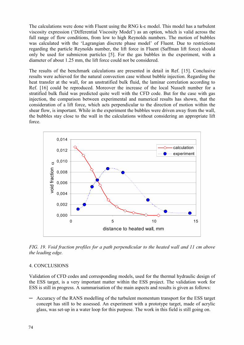
The calculations were done with Fluent using the RNG k-ε model. This model has a turbulent viscosity expression (‘Differential Viscosity Model’) as an option, which is valid across the full range of flow conditions, from low to high Reynolds numbers. The motion of bubbles was calculated with the ‘Lagrangian discrete phase model’ of Fluent. Due to restrictions regarding the particle Reynolds number, the lift force in Fluent (Saffman lift force) should only be used for submicron particles [5]. For the gas bubbles in the experiment, with a diameter of about 1.25 mm, the lift force could not be considered.

The results of the benchmark calculations are presented in detail in Ref. [15]. Conclusive results were achieved for the natural convection case without bubble injection. Regarding the heat transfer at the wall, for an unstratified bulk fluid, the laminar correlation according to Ref. [16] could be reproduced. Moreover the increase of the local Nusselt number for a stratified bulk fluid was predicted quite well with the CFD code. But for the case with gas injection, the comparison between experimental and numerical results has shown, that the consideration of a lift force, which acts perpendicular to the direction of motion within the shear flow, is important. While in the experiment the bubbles were driven away from the wall, the bubbles stay close to the wall in the calculations without considering an appropriate lift force.

0,000

0,002

0,004

0,006

0,008

0,010

0,012

0,014

0 5 10 15

distance to heated wall, mm

void

frac

tion

α

calculationexperiment

FIG. 19. Void fraction profiles for a path perpendicular to the heated wall and 11 cm above the leading edge.

4. CONCLUSIONS

Validation of CFD codes and corresponding models, used for the thermal hydraulic design of the ESS target, is a very important matter within the ESS project. The validation work for ESS is still in progress. A summarisation of the main aspects and results is given as follows:

─ Accuracy of the RANS modelling of the turbulent momentum transport for the ESS target concept has still to be assessed. An experiment with a prototype target, made of acrylic glass, was set-up in a water loop for this purpose. The work in this field is still going on.

74

─ With respect to heat transfer modelling, CFD codes are in principal able to predict the wall cooling for HLM flows with engineering accuracy if certain ancillary conditions are considered.

─ The Eulerian-Lagrangian two-phase flow modelling approach seems to be in principle suitable, to predict bubble trajectories within the ESS target. But to predict the bubble behaviour in the shear flow close to the wall correct, a suitable lift force is needed. More validation work is needed in this field. For more complex questions, like bubble separation or coalescence, as well as contact of bubbles with walls, new experiments are necessary in any case.

REFERENCES

[1] EUROPEAN COMMISSION, 5th Euratom Framework Programme 1998–2002, Key Action: Nuclear Fission, ASCHLIM, FIKW-CT2001-80121, 1 January–31 December 2002.

[2] BUCENIEKS, I., et al., ESS Mercury Target Model Experiment: Investigation on the Heat Transfer, European Spallation Source tech. Rep. ESS 98-73-T (1998).

[3] CORDS, H., A literature survey on fluid flow data for mercury, ESS 98-81-T (1998).[4] WOLTERS, J., Benchmark Activity on the ESS Mercury Target Model

Experiment, Forschungszentrum Jülich GmbH, Central Department of Technology, FZJ-ZAT-377, (December 2002).

[5] Fluent, release 5.5, Documentation Fluent Incorporated (2000), see also: http://www.fluent.com/news/pr/pr17.htm

[6] STAR-CD release 3.15: Methodology, Computational Dynamics (2001). [7] AEA Technology, CFX 4.2: Solver, CFX International, Harwell, U.K., (1997). [8] ARAGONESE, C., et al., Benchmark Calculation of Mercury Flow Experiments

Performed in Riga for the ESS Target, CRS4 Rechnical Report 99/21 (1999). [9] SICCAMA, N.B., KONING, H., Post-Test CFD Analysis of the ESS-HETSS

Experiment, NRG report 20923/02.49188/C. [10] KAYS, W.M., Turbulent Prandtl Number — Where Are We?, J. Heat Transfer, 116

(1994) pp. 284–295. [11] JISCHA, M., RIEKE, H.B., Modelling assumptions for turbulent heat transfer, Proc.

7th Int. Heat Transfer Conv., Munich (ed. U. Grigall et. al.), Vol. 4 (1982). [12] CLIFT, R., GRACE, J.R., WEBER, M.E., Bubbles, Drops and Particles, Academic

Press, San Diego, CA (1978). [13] WOLTERS, J., BULIGINS, L., ABÁNADES, A., ESTEBAN, G., PEÑA, A.,

Natural Convection Heat Transfer Enhancement in Mercury with Gas Injection & Benchmark ASCHLIM, 5th Euratom Framework Programme 1998–2002, Key Action: Nuclear Fission, April–August 2003 (to be published).

[14] TOKUHIRO, A., Natural Convection Heat Transfer Enhancement in Mercury with Gas Injection and in the Presence of a Transverse Magnetic Field, PH.D. Thesis, Purdue University, West Lafayette, IN (1991).

[15] WOLTERS, J., Benchmark Activity on Natural Convection Heat Transfer Enhancement in Mercury with Gas Injection, Forschungszentrum Jülich GmbH, Central Department of Technology, FZJ-ZAT-379 (2003).

[16] UOTANI, M., Natural Convection Heat Transfer in Thermally Stratified Liquid Metal, Journal of Nuclear Science and Technology, 24, Vol. 6 (June 1987) pp. 442–451.

75

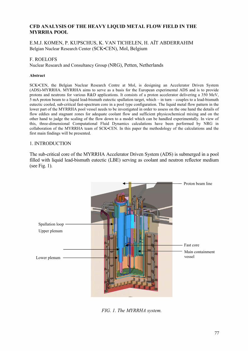
CFD ANALYSIS OF THE HEAVY LIQUID METAL FLOW FIELD IN THE MYRRHA POOL

E.M.J. KOMEN, P. KUPSCHUS, K. VAN TICHELEN, H. AÏT ABDERRAHIM Belgian Nuclear Research Center (SCK•CEN), Mol, Belgium

F. ROELOFS Nuclear Research and Consultancy Group (NRG), Petten, Netherlands

Abstract

SCK•CEN, the Belgian Nuclear Research Centre at Mol, is designing an Accelerator Driven System (ADS)-MYRRHA. MYRRHA aims to serve as a basis for the European experimental ADS and is to provide protons and neutrons for various R&D applications. It consists of a proton accelerator delivering a 350 MeV, 5 mA proton beam to a liquid lead-bismuth eutectic spallation target, which – in turn – couples to a lead-bismuth eutectic cooled, sub-critical fast-spectrum core in a pool type configuration. The liquid metal flow pattern in the lower part of the MYRRHA pool vessel needs to be investigated in order to assess on the one hand the details of flow eddies and stagnant zones for adequate coolant flow and sufficient physicochemical mixing and on the other hand to judge the scaling of the flow down to a model which can be handled experimentally. In view of this, three-dimensional Computational Fluid Dynamics calculations have been performed by NRG in collaboration of the MYRRHA team of SCK•CEN. In this paper the methodology of the calculations and the first main findings will be presented.

1. INTRODUCTION

The sub-critical core of the MYRRHA Accelerator Driven System (ADS) is submerged in a pool filled with liquid lead-bismuth eutectic (LBE) serving as coolant and neutron reflector medium (see Fig. 1).

FIG. 1. The MYRRHA system.

Proton beam line

Spallation loop Upper plenum

Lower plenum

Fast core Main containmentvessel

77

The roughly 60 m3 or 600 t of LBE fill a vessel of about 4 m inner diameter and 6 m height. Under full operation conditions, the LBE is “cold” at about 200°C in the lower part and flows through the central core upwards being heated to about 350°C on average. This “hot” zone is separated by a diaphragm (septum wall) from the “cold” zone, represented by the approximately 2 m high lower space. A total of 4 eccentrically positioned pumps force the circulating flow downwards through heat exchangers and provide the pressure head for the core cooling.

Since the lower pool is quite spacious to permit the loading of the core and exchange of fuel, the question arose whether the flow pattern in the lower part would behave benignly or contain unexpected flow eddies and/or stagnant zones. Such features could influence the cooling or the physico-chemistry of the LBE that is corrosive against the steel intended for use. The latter will be protected by proper dynamic oxygen control of the LBE whose concentration may not be controllable if sufficient mixing is not warranted.

2. OBJECTIVES

In the first instance, to assess the detailed flow pattern for adequate cooling and sufficient physico-chemical mixing, the basic isothermal flow pattern in the lower part of the vessel needs to be evaluated for the full size device in normal and abnormal operating conditions. This will already allow first conclusions to be drawn. The CFD analyses will be extended later on to cases where hot injection takes place – e.g. due to breakdown of the HEX cooling but continued pumping. And finally the full thermal cycle may be modeled.

Secondly, although the CFD results will be used as a guideline, according experiments are still necessary but are not economically possible at the scale of the planned device. Therefore, the lower part of the MYRRHA pool vessel needs to be scaled down by a linear factor of up to 10 which would enable to build a model which would contain now 60 L instead of 60 m3 of LBE. In view of this, a scaling method preserving the relevant flow features should be defined.

3. GEOMETRY

The lower pool space of MYRRHA to be modeled here is a cylindrical space of 4 m inner diameter and a height of approximately 2 m. The bottom surface is covered by a unit that provides electrical heating and process gas injection for oxygen control. Both functions are not of relevance here but the surface roughness of this structure has been taken into account. The same is true for top boundary which consists of grid to prevent detached objects to float into trapping spaces of the diaphragm.

The lower pool unit hangs from the diaphragm and the four support stanchions for pump and heat exchanger units are to be modeled in case they present obstacles to azimuthally developing flow by virtue of pump unbalances. A further asymmetric obstacle is introduced by the spallation loop. The coupling between the spallation loop and the lower pool through the spallation loop heat exchanger is not modelled. The inlet mass flow rate of the injecting pumps has been taken as 350 kg/s for each injecting pump through a nozzle of 200 mm diameter.

4. SCALING METHODS

The turbulent jets leaving the four pump units determine the flow pattern. Three different scaling methods are considered, based on different importance granted to the physical parameters characterizing a jet:

78

─ The turbulent jet is characterized by the Reynolds number with the pool diameter as characteristic length. In this case, the jets emerging from the down-scaled nozzles are equivalent to the jets emerging from the original nozzle when the velocity is increased.

─ The time a jet needs to reach the bottom of the MYRRHA pool is considered characteristic for the jet. The inlet velocity is now scaled by the same factor as the geometry.

─ The velocity of the jet at the pump outlet characterizes the jet. At the same time, the volume throughput time is kept constant.

The correct choice for the scaling method is not obvious and depends on the phenomena investigated. In case of physico-chemistry effects, time scales are of main importance and emphasis will be put on the correct representation of residence times. The three methods are summarized in Table 1.

TABLE 1. SCALING METHODS

Scaling

method

Inlet

diameter,

Pool

diameter,

Inlet

area,

Pool

volume,

Volume

flow,

Inlet

velocity,

Through-

put time,

Reynolds

number,

m m m² m³ m³/s m/s s -

Reynolds 1/f 1/f 1/f² 1/f³ 1/f f 1/f² 1

Characteristic

time

1/f 1/f 1/f² 1/f³ 1/f³ 1/f 1 1/f²

Inlet velocity 1/f3/2 1/f 1/f³ 1/f³ 1/f³ 1 1 1/f

5. CASES

The flow topology is analyzed for various scenarios, with special emphasis on the presence of stagnant zones. In the base case scenario, all four pumps have equal performance. For cases 1a through 1f, one or two pumps are stopped with no through-put permitted, the other pumps have equal performances per pump as compared to the base case. This is operationally not correct since the flow rates of the operating pumps would be increased. However, it will provide the design team with useful information about the residence times for each scenario.

The model is scaled down by a factor of 5 for the cases 2a and 2b. The scaling of the model is based on Reynolds numbers in case 2a, whereas the scaling of the model is based on a characteristic time in case 2b. The cases are summarized in Table 2.

79

TABLE 2. CASES

Case Case description

Base no pump tripping and no scaling 1a full scale, 1 pump close to the spallation loop tripped 1b full scale, 1 pump opposite of the spallation loop tripped 1c full scale, 2 pumps close to the spallation loop tripped 1d full scale, 2 pumps opposite of the spallation loop tripped

1e full scale, 1 pump close to the spallation loop and 1 pump opposite of the spallation loop, but close to the first pump, tripped

1f full scale, 1 pump close to the spallation loop and 1 pump opposite of the spallation loop, but diagonally opposite to the first pump, tripped

2a scaled down by a factor of 5, scaling based on Reynolds number 2b scaled down by a factor of 5, scaling based on characteristic time

6. CFD MODEL

6.1. Computer code

The computations have been performed using the widely used commercial CFD code CFX5.5 [2].

6.2. Mesh

The mesh for the lower MYRRHA pool model consists of 911 000 hexahedral computational cells. The k-ε turbulence model in combination with scalable wall functions as implemented in CFX5 has been selected for the current analyses. Therefore, the mesh refinement near the walls should ideally be such that the non-dimensionless distance y+ is larger than 12, in order to model the boundary layers. However, the wall friction is predicted with sufficient accuracy for this application, even for lower values of y+ [3]. For the full-scale model, the values of y+ are in the range of 20 to 200. For the scaled down model, the values of y+ are in the range of 4 to 20.

6.3. Main fluid dynamics model

The main fluid dynamics model describes a single-phase steady state time-averaged incompressible turbulent flow. The k-ε turbulence model in combination with scalable wall functions as implemented in CFX5 [2] has been selected in order to model turbulence. The MYRRHA core has been modeled by a porous medium, such that the pressure drop over the core is in accordance to the actual pressure drop [4] although this may cause a non-physical velocity profile at the core entrance which has to be considered with some prudence. It is judged, however, that the velocity profile at the core entrance has negligible influence on the locations in the flow field where the maximum residence times occur.

6.4. Properties

For the density and the dynamic viscosity of liquid lead-bismuth, constant properties have been used at a temperature of 473 K, as obtained from [5].

80

6.5. Boundary conditions

At the outlets of the pump sections, the inlet boundary conditions of the CFD model are specified. The prescribed mass flow rate of each pump in the full-scale model is 350 kg/s. At the outlet of the MYRRHA core, the static pressure is prescribed, whereas zero normal gradients are used for all remaining flow variables. In the full-scale model, at the bottom and upper plates of the lower MYRRHA pool, no-slip boundary conditions are specified with a wall roughness of 10 mm (for the full scale model). All other walls are considered as smooth walls with no-slip boundary conditions.

7. RESULTS

In the first instance, the flow topology of the heavy liquid metal is analyzed with emphasis on the presence of flow eddies and stagnant zones in order to evaluate the basic isothermal flow pattern in the lower part of the vessel for the full size device in normal and abnormal operating conditions. The maximum residence times of lead-bismuth in the MYRRHA pool as observed in the analyses are presented in Table 3.

TABLE 3. MAXIMUM RESIDENCE TIME FOR THE BASE CASE AND CASES 1a THROUGH 1f

Case Maximum residence time [s]

Base 280

1a 430

1b 360

1c 590

1d 560

1e 630

1f 600

The maximum residence time increases with the number of pumps that are stopped. For the base case, in which all pumps are functioning, the maximum residence time is 280 s (as compared to the nominal value of 190 s that one would arrive at in dividing the exchange volume of about 25 m3 by the through-put of all 4 pumps of 1400 kg/s). For 1 pump stopped, the maximum residence time increases to approximately 430 s, whereas for 2 pumps stopped, the maximum residence time increases to approximately 600 s. This increase of residence time with the number of pumps that are stopped is caused by the decreased total mass flow rate, since each stopped pump causes the total mass flow rate to decrease with 350 kg/s. Comparison of cases 1a and 1b on the one hand and cases 1c through 1f on the other hand, shows that the variation of the maximum residence time as a result of the mass flow rate distribution is approximately 15%. The occurrence of the physicochemical effects and precipitation has a typical time-scale of several days. Compared to this, the maximum residence times resulting from the analyses are more than a factor 100 lower. Iso-surfaces of residence time are presented in Fig. 2. This figure indicates which pumps are functioning and which are not functioning.

81

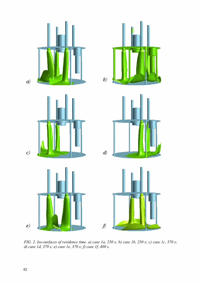
FIG. 2. Iso-surfaces of residence time. a) case 1a, 250 s; b) case 1b, 250 s; c) case 1c, 370 s; d) case 1d, 370 s; e) case 1e, 370 s; f) case 1f, 400 s.

82

In Fig. 3, iso-surfaces of residence time are presented, indicating the locations in the pool where the maximum residence times occur.

FIG. 3. Iso-surfaces of residence time. a) case 1a, 380 s; b) case 1b, 340 s; c) case 1c, 580 s; d) case 1d, 550 s; e) case 1e, 590 s; f) case 1f, 580 s.

83

Typically, the largest residence time occur in the upper corners of the pool, where the side-walls meet the upper grid, near the upper grid and near the target loop. The latter evidence might change for the better if the spallation loop heat exchanger were modeled because that flow does represent some 7% of the total through-put. Secondly, in order to compare results obtained with various scaling methods, a dimensionless velocity and dimensionless residence time are defined. The dimensionless velocity (v’) is obtained by dividing the velocity (v) by the inlet velocity (vinlet):

inletvvv ='

The inlet velocity is obtained from the specified mass flow rate at the pump outlets, the pump outlet area and the density of the applied fluid. The dimensionless residence time (t’res) is obtained by dividing the residence time (tres) by a characteristic time:

)/('

inletpool

resres vD

tt =

where

Dpool is the diameter of the pool.

The maximum dimensionless residence times of lead-bismuth in the MYRRHA pool as observed in the analyses are presented in Table 4. Where the characteristic time based scaling (case 2b) leads to practically equal maximum residence times compared to the base case, the maximum residence time for the Reynolds number based scaling (case 2a) exceeds the maximum residence time of the base case by approximately 22%. However, the occurrence of the physico-chemical effects and precipitation has a typical time-scale of several days. Compared to this, even the maximum residence times resulting from the Reynolds number based scaling analyses are much more than a factor 100 lower.

TABLE 4. MAXIMUM DIMENSIONLESS RESIDENCE TIME FOR THE BASE CASE AND CASES 2a and 2b

Case Maximum dimensionless residence time [-]

Base 73

2a 89

2b 72

The flow fields for the base case and cases 2a and 2b are presented in Fig. 4. Within this figure, figures a, c, and e present contours of dimensionless velocity, whereas the other figures present contours of dimensionless residence times. The flow direction is indicated using scaled velocity vectors. The flow fields of the base case and case 2a are comparable. The flow fields of the base case and case 2b are practically similar. However, the similarity between the base case and case 2a (Reynolds number based scaling) is less than the similarity between the base case and case 2b (characteristic time based scaling).

84

FIG. 4. Flow field of the base case (a & b), case 2a (c & d), and case 2b (e & f). The contours in figures a, c, and e indicate dimensionless velocity. The contours in figures b, d, and f indicate dimensionless residence time.

85

Iso-surfaces of dimensionless residence time are presented in Fig. 5.

FIG. 5. Iso-surfaces of dimensionless residence time of the base case (a & b), case 2a (c & d), and case 2b (e & f). The dimensionless residence time in figures a, c, and e equals 45.8. The dimensionless residence time in figure b equals 72.7, in figure d equals 83.0, and of figure f equals 68.0.

86

Within this figure, figures a, c, and e present iso-surfaces of a dimensionless residence time equal to 45.8, whereas the residence time in the other figures is chosen such that the figure indicates the locations of the largest residence times. The figure shows that the locations of maximum residence time are practically similar for the base case and case 2b. Compared to this, there is less similarity between the locations of maximum residence time of the base case and case 2a.

8. CONCLUSIONS AND OUTLOOK

From the isothermal calculations in the lower part of the MYRRHA pool vessel, it is clear that - even in abnormal operational conditions with two pumps failing - the flow pattern behaves well: it does not contain long-term flow eddies and/or stagnant zones which could influence the cooling or physico-chemistry of the LBE. In the future, the CFD analyses will be extended to cases were hot injection takes place and finally the full thermal cycle may be modeled.

From the present scaling analyses it is concluded that scaling all dimensions by a factor of 5 hardly changes the characteristic residence times with respect to the time-scales for physico-chemical effects, both for the Reynolds- and time-based strategies. It is expected that the same is true for the velocity based scaling. This will be confirmed in the near future. One can expect from the current results that even larger scaling factors, leading to smaller and thus less expensive experiments, are possible without affecting drastically the time scales. In view of this, a sensitivity study is planned. This will provide an optimal scaling factor for a ‘small’-size experiment in which physico-chemical effects will be studied.

REFERNCES

[1] AÏT ABDERRAHIM, et al., MYRRHA, A Multipurpose Accelerator Driven System for R&D. State-of-the-art mid 2003, Proc. International Workshop on P&T and ADS Development, SCK•CEN, BLG-959, ISBN 9076971072, Mol, Belgium (2003).

[2] CFX5 USER GUIDE, AEA Technology, Harwell, U.K. (1999). [3] VIESER, W., ESH, T. & MENTER, F., Heat Transfer Predictions using Advanced

Two-Equation Turbulence Models, CFX Validation Report CFX-VAL10/0602 (2002).[4] KUPSCHUS, P., Vessel layout c/w/ spallation, private communication 2003. [5] VAN TICHELEN, K., Lead-Bismuth Properties Database, SCK•CEN Report

RF&M/KVT/kvt/32.B043000/85/01-47, Mol, Belgium (2001).

87

COMPARATIVE ANALYSIS OF THE BENCHMARK ACTIVITY RESULTS ON THE ADS TARGET MODEL

A. SOROKIN, G. BOGOSLOVSKAIA, V. MIKHIN, S. MARZINUK State Scientific Center, Institute for Physics and Power Engineering (SSC RF-IPPE), Obninsk, Russian Federation

Abstract

Benchmark activity on the heat exchange in the Accelerator Driven System (ADS) target model had been conducted in the frame of the International Meeting of the Working Group on Advanced Nuclear Reactors Thermohydraulics in the frame of the International Association for Hydraulic Engineering and Research. The specialists of IPPE had prepared the task on the benchmark activity using the experimental data. The specialists of Japan, Spain and China had participated in the benchmark activity. Also the calculation results had been received by the specialists of Italy and Russia. There is a considerable divergence between the calculated membrane temperature distributions as well as between the calculated and experimental one. The more reliable approaches of simulating the distributing grid and heat generation and also turbulence generation due to the jet interactions behind the distributing grid are needed for precise prediction of the membrane temperature.

1. INTRODUCTION

Benchmark activity on the heat exchange in the Accelerator Driven System (ADS) target model had been conducted in the frame of the International Meeting of the Working Group on Advanced Nuclear Reactors Thermohydraulics of the International Association for Hydraulic Engineering and Research, which had taken place in 17–19 July 2001 in Obninsk, on the base of the IPPE. The specialists of IPPE had prepared the task on the benchmark activity using the experimental data of IPPE on the heat exchange in the ADS target model [1]. Tree researcher group had participated in the benchmark activity from: Japan [2], Spain [3], and China [4]. Later the calculation results of the specialists of Italy and Russia had been received also.

2. THE EXPERIMENTAL RESULTS AND CONDITIONS

The test model, representing it self as an axially symmetric construction installed on the liquid-metal test facility AP-1 was created for carrying out the experiments is shown in Fig 1.

1 - copper unit with nickel-chrom-heaters 2 - membrane of the target 3 - grid with profiling holes 4 - thermocouple block

FIG. 1. Experimental device.

Outlet Inlet

89

The coolant was directed upwards in the horizontal, outer, annular test-model channel. Striking against the membrane surface the coolant turned and passed through the distributing grid (see Fig. 2) into the inner channel (tube). Then it returned through the socket in the bottom part of the tube back on the inlet of the re-circulating pump.

FIG. 2. Distribution grid.

The membrane represented it self as a thin shaped plate with a thickness 1.5 mm and made of stainless steel. The heat flow on the membrane surface was created by means of the copper rod with the diameter 65 mm and with its butt-end soldered with silver to the membrane surface. The heating of the rod was realized by the wedge-shaped-heating method.

The heating block represented a copper pig of the diameter 130 mm and length 200 mm in which 19 holes with the diameter 19 mm and depth 200 mm were perforated. Ceramic bushes being 19 mm in diameter and made of magnesium oxide were inserted in the block holes. Every ceramic bush had four holes intended for installing the heating coils and having the diameter equal to 4 mm. The coils made of nichrome wire 1.2 mm in diameter could be engaged in the consecutive or parallel circuit. The heating block was in the chamber filled with helium that improved the heater performance due to the high heat conductivity and prevented the copper block oxidation at higher temperatures. The eutectic sodium-potassium alloy having the Prandtl number close to the lead-bismuth Prandtl number was used as the coolant.

90

In the experimental investigations the following parameters were measured: inlet and outlet flow temperature; coolant rate; energy-release power; heat flow conducted to the membrane; radial temperature distribution on the membrane surface from the coolant side; radial temperature distributions in the coolant in the inner tube; axial temperature distributions in the coolant in the inner tube and in the space between the membrane and distributing grid; coolant temperature fluctuations.

The radial temperature distributions in the inner tube were measured in two different directions: vertical and horizontal. The measurements were done with the help of the mobile thermocouple block [12] (see Fig. 1).

The mobile thermocouple block represented it self two orientated mutually perpendicular combs with the thermocouples arranged opposite the corresponding holes of the distributing grid [11] (see Fig. 2). Instantaneous temperature values were measured by placing the thermocouple block in the different cross-sections in the inner channel (as well as in the space between the membrane and distributing grid) away from the membrane surface at distances 15, 20, 40, 60, 80, 100, 150, 200, 250, and 300 mm. The narrow jet of the hot coolant as well as the large coolant temperature fluctuations was observed in the inner channel downstream from the distributive grid.

The radial temperature distribution on the membrane surface was measured with using the mobile thermocouple. The thermocouple was moved in a capillary of 0.6 mm in diameter placed in the special groove made on the membrane surface from the coolant side. These data were obtained by using the mobile thermocouple placed in the capillary in the vertical groove in the membrane surface adjacent with the coolant.

The data on the instantaneous values of the membrane surface temperature characterizing by the high level of the temperature fluctuations were obtained.

Measurements were realized with using the system of automatic data collection and processing.

3. CODES AND MODELS USED IN TEST CALCULATION [2–7]

Together with the three-dimensional approach [2, 3] the two-dimensional approximation of the problem assuming the axial symmetry of the system was used also [3–6]. The three-dimensional simulation of the problem had been performed by means of AQUA code [2] and commercial FLUENT code [2, 3].

Table 1 shows the codes and turbulence models used in test calculations.

91

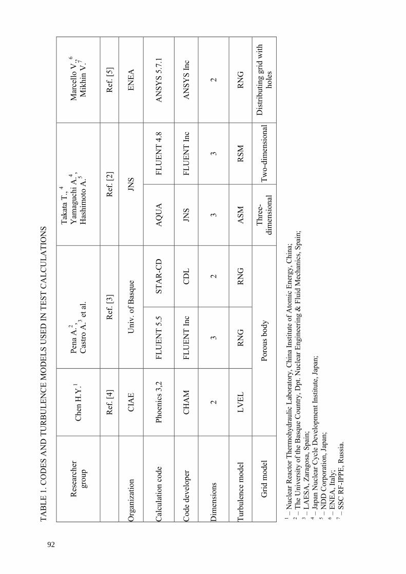
TAB

LE 1

. CO

DES

AN

D T

UR

BU

LEN

CE

MO

DEL

S U

SED

IN T

EST

CA

LCU

LATI

ON

S

Res

earc

her

grou

p C

hen

H.Y

.1 Pe

na A

.2 , C

astro

A.3 e

t al.

Taka

ta T

., 4

Yam

aguc

hi A

.4 , H

ashi

mot

o A

.5

Mar

cello

V.,6

Mik

hin

V.7

R

ef. [

4]

Ref

. [3]

R

ef. [

2]

Ref

. [5]

Org

aniz

atio

n C

IAE

Uni

v. o

f Bas

que

JNS

ENEA

Cal

cula

tion

code

Ph

oeni

cs 3

,2

FLU

ENT

5.5

STA

R-C

D

AQ

UA

FL

UEN

T 4.

8 A

NSY

S 5.

7.1

Cod

e de

velo

per

CH

AM

FL

UEN

T In

c C

DL

JNS

FLU

ENT

Inc

AN

SYS

Inc

Dim

ensi

ons

2 3

2 3

3 2

Turb

ulen

ce m

odel

LV

EL

RN

G

RN

G

ASM

R

SM

RN

G

Grid

mod

el

Poro

us b

ody

Thre

e-di

men

sion

al

Two-

dim

ensi

onal

Dis

tribu

ting

grid

with

ho

les

1 – N

ucle

ar R

eact

or T

herm

ohyd

raul

ic L

abor

ator

y, C

hina

Inst

itute

of A

tom

ic E

nerg

y, C

hina

;

2 – T

he U

nive

rsity

of t

he B

asqu

e C

ount

ry, D

pt. N

ucle

ar E

ngin

eerin

g &

Flu

id M

echa

nics

, Spa

in;

3 – L

AES

A, Z

arag

osa,

Spa

in;

4 – Ja

pan

Nuc

lear

Cyc

le D

evel

opm

ent I

nstit

ute,

Japa

n;

5 – N

DD

Cor

pora

tion,

Japa

n;

6 – E

NEA

, Ita

ly;

7 – S

SC R

F-IP

PE, R

ussi

a.

92

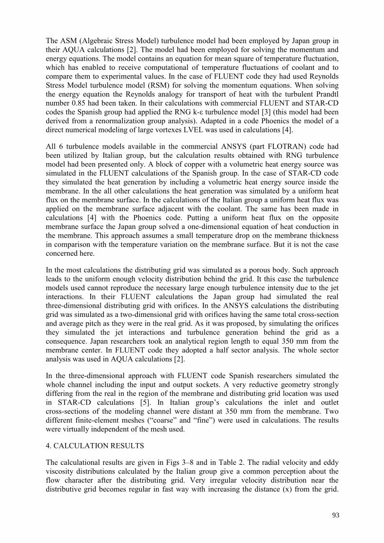
The ASM (Algebraic Stress Model) turbulence model had been employed by Japan group in their AQUA calculations [2]. The model had been employed for solving the momentum and energy equations. The model contains an equation for mean square of temperature fluctuation, which has enabled to receive computational of temperature fluctuations of coolant and to compare them to experimental values. In the case of FLUENT code they had used Reynolds Stress Model turbulence model (RSM) for solving the momentum equations. When solving the energy equation the Reynolds analogy for transport of heat with the turbulent Prandtl number 0.85 had been taken. In their calculations with commercial FLUENT and STAR-CD codes the Spanish group had applied the RNG k-ε turbulence model [3] (this model had been derived from a renormalization group analysis). Adapted in a code Phoenics the model of a direct numerical modeling of large vortexes LVEL was used in calculations [4].

All 6 turbulence models available in the commercial ANSYS (part FLOTRAN) code had been utilized by Italian group, but the calculation results obtained with RNG turbulence model had been presented only. A block of copper with a volumetric heat energy source was simulated in the FLUENT calculations of the Spanish group. In the case of STAR-CD code they simulated the heat generation by including a volumetric heat energy source inside the membrane. In the all other calculations the heat generation was simulated by a uniform heat flux on the membrane surface. In the calculations of the Italian group a uniform heat flux was applied on the membrane surface adjacent with the coolant. The same has been made in calculations [4] with the Phoenics code. Putting a uniform heat flux on the opposite membrane surface the Japan group solved a one-dimensional equation of heat conduction in the membrane. This approach assumes a small temperature drop on the membrane thickness in comparison with the temperature variation on the membrane surface. But it is not the case concerned here.

In the most calculations the distributing grid was simulated as a porous body. Such approach leads to the uniform enough velocity distribution behind the grid. It this case the turbulence models used cannot reproduce the necessary large enough turbulence intensity due to the jet interactions. In their FLUENT calculations the Japan group had simulated the real three-dimensional distributing grid with orifices. In the ANSYS calculations the distributing grid was simulated as a two-dimensional grid with orifices having the same total cross-section and average pitch as they were in the real grid. As it was proposed, by simulating the orifices they simulated the jet interactions and turbulence generation behind the grid as a consequence. Japan researchers took an analytical region length to equal 350 mm from the membrane center. In FLUENT code they adopted a half sector analysis. The whole sector analysis was used in AQUA calculations [2].

In the three-dimensional approach with FLUENT code Spanish researchers simulated the whole channel including the input and output sockets. A very reductive geometry strongly differing from the real in the region of the membrane and distributing grid location was used in STAR-CD calculations [5]. In Italian group’s calculations the inlet and outlet cross-sections of the modeling channel were distant at 350 mm from the membrane. Two different finite-element meshes (“coarse” and “fine”) were used in calculations. The results were virtually independent of the mesh used.

4. CALCULATION RESULTS

The calculational results are given in Figs 3–8 and in Table 2. The radial velocity and eddy viscosity distributions calculated by the Italian group give a common perception about the flow character after the distributing grid. Very irregular velocity distribution near the distributive grid becomes regular in fast way with increasing the distance (x) from the grid.

93

The large eddy viscosity produced by the jet interactions and making up a few order of the molecular one explains such behavior of the velocity distributions (Fig. 3).

0,00

0,02

0,04

0,06

0,08

X=0.023

0,00

0,02

0,04

0,06

0,08

X=048

0,00

0,04

0,08

0,12

X=0.1

μt

0,00

0,04

0,08

0,12

X=0.15

0,00 0,01 0,02 0,03 0,04 0,05 0,060,00

0,05

0,10

0,15

0,20

0,25

X=0.2

r0,00 0,01 0,02 0,03 0,04 0,05 0,06

0,00

0,05

0,10

0,15

0,20

0,25

X=0.35

r

FIG. 3. Profiles of the eddy viscosity in the inner tube at the different distances from the membrane.

The experimental data show non-monotone radial variation of the membrane temperature with the temperature increase in the membrane periphery direction (Fig. 4).

FIG. 4. Temperature distributions on the membrane surface (y is the distance from the membrane axis).

94

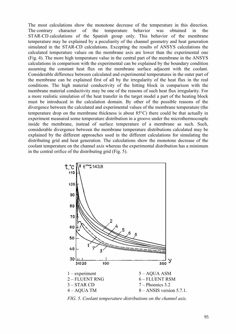
The most calculations show the monotone decrease of the temperature in this direction. The contrary character of the temperature behavior was obtained in the STAR-CD calculations of the Spanish group only. This behavior of the membrane temperature may be explained by a peculiarity of the channel geometry and heat generation simulated in the STAR-CD calculations. Excepting the results of ANSYS calculations the calculated temperature values on the membrane axis are lower than the experimental one (Fig. 4). The more high temperature value in the central part of the membrane in the ANSYS calculations in comparison with the experimental can be explained by the boundary condition assuming the constant heat flux on the membrane surface adjacent with the coolant. Considerable difference between calculated and experimental temperatures in the outer part of the membrane can be explained first of all by the irregularity of the heat flux in the real conditions. The high material conductivity of the hitting block in comparison with the membrane material conductivity may be one of the reasons of such heat flux irregularity. For a more realistic simulation of the heat transfer in the target model a part of the heating block must be introduced in the calculation domain. By other of the possible reasons of the divergence between the calculated and experimental values of the membrane temperature (the temperature drop on the membrane thickness is about 85°C) there could be that actually in experiment measured some temperature distribution in a groove under the microthermocouple inside the membrane, instead of surface temperature of a membrane as such. Such, considerable divergence between the membrane temperature distributions calculated may be explained by the different approaches used in the different calculations for simulating the distributing grid and heat generation. The calculations show the monotone decrease of the coolant temperature on the channel axis whereas the experimental distribution has a minimum in the central orifice of the distributing grid (Fig. 5).

1 – experiment 5 – AQUA ASM 2 – FLUENT RNG 6 – FLUENT RSM 3 – STAR CD 7 – Phoenics 3.2 4 – AQUA TM 8 – ANSIS version 5.7.1.

FIG. 5. Coolant temperature distributions on the channel axis.

95

But there is no considerable difference between the calculated and experimental radial coolant temperature distributions except the points at the channel axis. The heat flux irregularity in the real conditions leading to the relatively low temperature on the central point of the membrane may be a reason of such difference at the points on the channel axis with z ≤ 80 mm. Dissymmetry of the real flow in the inner tube is likely to be a reason of the difference in the distributions in the cross-sections with z ≥ 100 mm (z is a distance from the membrane).

The coolant temperature fluctuation near to membranes surface obtained by Japanese specialists with the AQUA-ТМ calculations are close to experimental (distance from the membrane 1 mm). The maximum temperature fluctuations on mid-channels obtained in experiment and in calculations, are equal 7.8 and 9.5°С, accordingly. However, computational data for an internal channel are much higher experimental. For example, on distance of 10 mm from a membrane the computational maximum temperature fluctuation (8.9°С) is approximately twice higher experimental (3.6°С) and approximately in 5 times above experimental for distance from a membrane of 300 mm-1.3 and 5.8°С, accordingly. While the experimental temperature fluctuations of decrease with increase of distance from a membrane, the computational values do not depend on this distance.

The coolant temperature distributions obtained by ANSYS code and Japanese specialists by FLUENT code are close one to other. The difference between the temperature values on the channel axis near the grid can be easily explained by the difference of heat fluxes simulated in the membrane center. There is also a similarity in the behavior of the membrane temperature distributions in spite of that the membrane temperatures calculated by the Japan group by FLUENT code are much lower than ones calculated by ANSYS code. The difference in values can be explained by errors in determination of the membrane temperature under an assumption that it meets a one-dimensional equation. This assumption is valid when the temperature drop on the membrane thickness is much smaller than the temperature variation on the membrane surface.

FIG. 6. Radial coolant temperature distributions: (distance between the membrane and thermocouple block is 1 mm).

96

The most interesting result of the ANSYS calculations probably is in the following. Only two turbulence models RNG and “Zero Equation Turbulence Model” had reproduced the necessary eddy viscosity generation due to the jet interactions behind the grid. The rest four available in the ANSYS code had given the zero eddy viscosity values nearly in the whole volume of the inner tube except a thin near-wall sub-layer.

Obtained by Spanish group the appreciably asymmetrical coolant temperature distributions even in the channel symmetry plane together with the temperature values about 5°C less than the inlet temperature show that they probably didn’t reach the convergent solution in the calculations with the FLUENT code.

FIG. 7. Radial coolant temperature distributions: (distance between the membrane and thermocouple block is 10 mm).

FIG. 8. Radial coolant temperature distributions: (distance between the membrane and thermocouple block is 100 mm).

97

TABLE 2. MEMBRANE TEMPERATURE (Y IS THE DISTANCE FROM THE MEMBRANE CENTER)

Y, mm EXPER FLUENТ RNG STAR-CD AQVA FLUENT

RSM Phoenics ANSYS

+30 11.8 72.9 143.6 70.8 57.4 68.6 67.4

+25 138.8 81.9 139.2 82.6 65.3 70.0 81.2

+20 119.8 86.9 125.1 89.1 72.2 78.2 89.6

+15 114.2 106 114.7 94.1 76.1 87.0 97.4

+10 108.4 107 109.6 95.1 85.1 99.8 110.4

+5 132.5 113 106.6 104.8 92.3 111.1 130.0

0 133.1 126 101.8 116.9 111.5 119.0 170.9

-5 121.3 123 106.6 102.6 92.1

-10 106.7 112 109.6 94.0 80.2

-15 110.3 104 114.7 93.7 76.3

-20 104.4 112 125.1 88.7 69.3

-25 131.5 86.9 139.2 82.5 63.1

-30 138.1 76.9 143.6 70.8 56.8

5. CONCLUSIONS

There is a considerable divergence between the calculated membrane temperature distributions as well as between the calculated and experimental one. The more reliable approaches of simulating the distributing grid and heat generation are needed for precise prediction of the membrane temperature. There is no considerable difference between the calculated and experimental values of the coolant temperature except the points at the channel axis. Dissymmetry of the real flow in the inner tube is likely to be a reason of such difference at the channel axis because the symmetric state of the flow in the inner tube seems to be extremely incredible. The benchmark participants have tested more turbulence models available in the codes than presented in Table 2.

Not all of the tested turbulence models have reproduced the turbulence generation due to the jet interactions behind the distributing grid.

98

REFERENCES

[1] ORLOV, YU., SOROKIN, A., BOGOSLOVSKAYA, G., et al., Specification on Benchmark Problem “Thermal Experiments in the ADS Target Model”, Proc. Meeting of International Working Group on Thermalhydraulics of Advanced Nuclear Reactors, Obninsk, Russia, 17–19 July 2001. In: Thermal hydraulics for Fast Reactors with Different Coolants, Obninsk, Russian Federation, IPPE (2003) pp. 207–235.

[2] TAKATA, T., YAMAGUCHI, A., HACHIMOTO, A., Benchmark Calculation of the Thermal Experiments in the ADS Target Model, Proc. Meeting of International Working Group on Thermalhydraulics of Advanced Nuclear Reactors, Obninsk, Russia, 17–19 July 2001. In: Thermal hydraulics for Fast Reactors with Different Coolants, Obninsk, Russian Federation, IPPE (2003) pp. 251–269.

[3] PEÑA, A., CASTRO, A., ESTEBAN, G.A., et al. Benchmark activities of UPV/EHU and LAESA concerning the TS-1 target system experiments, Proc. Meeting of International Working Group on Thermalhydraulics of Advanced Nuclear Reactors, Obninsk, Russia, 17–19 July 2001. In: Thermal hydraulics for Fast Reactors with Different Coolants, Obninsk, Russian Federation, IPPE (2003) pp. 236–250.

[4] CHEN, H.Y., Calculation results of the benchmark problem, Proc. Meeting of International Working Group on Thermalhydraulics of Advanced Nuclear Reactors, Obninsk, Russia, 17–19 July 2001. In: Thermal hydraulics for Fast Reactors with Different Coolants, Obninsk, Russian Federation, IPPE (2003) p. 270.

[5] MIKHIN, V., MARCELLO, V., Results of testing the ANSYS (part FLOTRAN) code in the ADS-target-model thermo-hydraulics calculations, ENEA, Italy, Bologna (2001).

[6] STAR-CD, version 3.1 User Manual. Computational Dynamics Limited (1999). [7] FLUENTS User’s guide. FLUENT Incorporated (1999), see also

http://www.me.mtu.edu/help/computing/docs/fluent/manuals/fluent5/ug/html/main_pre.htm

99

FREE SURFACE FLUID DYNAMICS CODE ADAPTATION BY EXPERIMENTAL EVIDENCE FOR THE MYRRHA SPALLATION TARGET

K. VAN TICHELEN Belgian Nuclear Research Center (SCK•CEN), Mol, Belgium Center for Nuclear Engineering, Leuven, Belgium

P. KUPSCHUS, M. DIERCKX, H. AÏT ABDERRAHIM Belgian Nuclear Research Center (SCK•CEN), Mol, Belgium

F. ROELOFS Nuclear Research and Consultancy Group (NRG), Petten, Netherlands

Abstract

For the spallation target of the MYRRHA Accelerator Driven System, under development at SCK•CEN, Mol, Belgium, a windowless design was chosen mainly for reasons of space limitations in the high-performance sub-critical core. This results in a challenging task for the MYRRHA spallation target design team: the design of a target nozzle in which a heavy liquid metal free surface flow is created within the geometrical constraints imposed by the sub-critical core, adequate to remove the heat deposited by the proton beam and compatible with the vacuum requirements of the beam transport system of the accelerator. A series of promising experiments have shown – in principle – the possibility of creation of an adequate flow pattern. The investigations, however, have also revealed a discrepancy between the experimental pattern and the one calculated with Computational Fluid Dynamics codes. These calculations are indispensable since proton beam heating cannot yet be simulated experimentally because of the lack of a suitable accelerator and neutron compatible experimental environment. Therefore, next to the experimental optimisation of the nozzle, the current research at SCK•CEN aims at reducing the discrepancy between code and experiment. This paper reports on the R&D program that takes this challenge.

1. BOUNDARY CONDITIONS FOR THE SPALLATION TARGET

At the heart of an Accelerator Driven System (ADS) is the spallation target. It is the source of primary neutrons that are multiplied by the surrounding sub-critical core. For the spallation target of the MYRRHA ADS [1] under development at SCK•CEN, liquid lead-bismuth eutectic (LBE) is chosen because of its good spallation neutron yield and low melting temperature allowing convective heat removal of the beam power at relatively low temperatures. Moreover, a windowless design was chosen, mainly for reasons of space limitations in the high-performance sub-critical core. These only permit a central hole of about Ø 120 mm, with about Ø 70 mm of target area. The proton current density of the 350 MeV, 5 mA beam therefore will exceed 150 µA/cm2. With a beam penetration depth of about 13 cm in the LBE, the deposited beam thermal power of 1.4 MW is dumped into 0.5 L from which it is removed by convection at a speed of 2.5 m/s, leading to an average temperature increase of less than 100°C, for an inlet flow of 10 L/s at 240°C.

The windowless target is formed from an annulus in the beam line in the centre of the sub-critical core through which the LBE flows a speed of 2.5 m/s (see Fig. 1). At the mid-level of the sub-critical core, the flow is directed into the central Ø 70 mm tube. The radially confluent flow forms secondary eddies on the free surface, of which the most fundamental eddy is a toroidal re-circulation with a central upwards component.

Since eddies are potential dead-water zones and have only limited exchange with the main flow, there is the danger that the beam will generate hot spots that are evaporating sufficient particles to jeopardize the beam transport vacuum (<10-3 mbar) and - in a subsequent run-away - the thermal capability of the beam transport system. In view of this, minimizing

101

the re-circulation zone is seen as a major tool to handle the surface hating. Moreover, the proton beam that comes from above, will be pencil-shaped and scans the target surface in the kHz-range in such a way that it best matches the re-circulation pattern of the free surface. It is suggested from estimates that the evaporation from ‘hot spots’ close to the free surface in the re-circulation zone is then still acceptable.

FIG. 1. Windowless spallation target.

2. INTRODUCTION TO THE PROBLEM

To gain insight in the characteristics and expertise in the creation of an adequate free surface flow, SCK•CEN has developed a roadmap of experiments supported and guided by Computational Fluid Dynamic (CFD) calculations. The CFD calculations are indispensable in order to investigate the flow pattern and temperature profile in the presence of beam heating which cannot be simulated experimentally at this stage due to the lack of a suitable accelerator and neutron compatible experimental environment.

Since to-scale experiments with LBE are more difficult to conduct, a series of promising experiments have been performed using the relatively easy-to-handle water and mercury as simulating fluids. (From hydrodynamic similarity considerations, these show far-going equivalence under the above target flow conditions. However, from the Prandtl number that describes the heath transfer capability of the liquids, it is clear that LBE experiments remain indispensable for analyzing the thermal aspects).

The experiments have shown – in principle – the possibility of creation of a stable and adequate free surface flow. The investigations, however, have also revealed a discrepancy between the experimentally observed free surface shape and flow pattern and the one calculated using CFD codes in relatively simple approximations (concerning surface and turbulent flow models).

In view of this, next to the experimental optimization of the nozzle, the aim of the current research at SCK•CEN is to reduce the discrepancy by widening the model options and adapting the codes by experimental evidence.

130

350 MeV × 5 mA BEAM (= 1.75 MW of which 80% is heat to be convectively removed)

120

Minimized recirculation zone (zone 1) (gets lower ‘tailored’ heat input)

Annular down-comer tube Beam line vacuum

72

High-speed zone (zone 2) (v ~ 2.5 m/s – permits effective heat removal)

102

3. EXPERIMENTS VERSUS COMPUTATIONS

3.1. First water experiments

3.1.1. Experimental observations

In June 1999 an R&D program started in collaboration with the thermal-hydraulics department of Université Catholique de Louvain (UCL, Belgium). Within this R&D program, water experiments on a one-to-one scale under atmospheric pressure were performed. Due to equipment limitations and the initial lower specification of the beam, most experiments were performed at a flow rate of 5 L/s. The velocity field was determined using LASER and ultrasonic Doppler measurements.

As result of the experimental investigations [2] a stable free surface at different fluid levels could be established. One could clearly observe two zones in the free surface region:

─ A conical zone with a relatively smooth free surface except for a small stochastic circumferential ripple on the surface with otherwise good axial symmetry (zone 2 in Fig. 1);

─ A recirculation zone with a whirling surface. A three-dimensional granular structure is apparent with fluid cells of about 5 mm in diameter moving over the surface at random with fluctuation frequencies in the order of 10 to 100 Hz (zone 1 in Fig. 1).

The water experiments did not allow optimization by minimizing the re-circulation zone as at a certain level, air from the atmosphere above is entrained in the flow leading to two-phase conditions with entirely different flow properties and patterns. This limited the usefulness of the water experiments under atmospheric pressure.

3.1.2. Computational observations - ASCHLIM

The first water experiments at UCL were subject of a benchmark activity within the 5th Framework Program of the European Commission – ASCHLIM [3]. The ASCHLIM project aimed at joining different experiences in the field of heavy liquid metals both in the experimental and numerical fields and creating an international collaboration to make an assessment of the main problems in the fields of turbulence, free surface and bubbly flow to coordinate future research activities.

Four different codes were used for the simulation of the water experiment with different approaches for free surface treatment: the interface-capturing or VOF (Volume of Fluid) codes FLOW-3D (single-fluid), FLUENT and COMET (two-fluids) and the interface-tracking codes for STAR-CD and COMET (moving-mesh). Axi-symmetry was assumed in all the cases. Turbulence was modelled using the k-ε method. Three test cases were calculated combining two different flow rates and two different free surface levels i.e. two different sizes of the re-circulation region.

Both interface-tracking methods appeared to be unable to simulate the low-surface case, for which the re-circulation zone is small and which is the desired one for the spallation target. They fail at the outer edge of the re-circulation zone where the mesh deformation is too large.

From the qualitative point of view, all VOF codes proved their ‘in-principle’ capability of simulating the global behaviour of the experiment, although they gave a somewhat smeared surface especially at the outer edge of the re-circulation zone. This is of course undesirable

103

since it will influence later on the temperature profile at the surface. The smearing was more pronounced for the two-fluid VOF codes. In view of this and due to the large density difference between the two fluids, it was concluded that one-fluid VOF codes are to be preferred.

A dome-shaped free surface was reproduced and the large re-circulation zone below the free surface appeared in all the calculations. However, the observed small-scale granular structure was not apparent, although it is of primary importance for the subsequent heat transfer calculations. Two possible causes for these shortcomings were identified: the reduction of the problem to an axi-symmetric case and inability of the k-ε turbulence model to capture the three-dimensional large-scale turbulent motions observed in reality.

From the quantitative point of view, the conclusions were not so positive. For the low-flow rate, high-level case, simulated with FLOW-3D, STAR-CD and FLUENT, the velocity profiles generally agreed rather well with the experimental results. Increasing the flow rate and/or lowering the surface level led to larger and larger discrepancies in the mean velocity profiles. In all cases, strong discrepancies in the turbulence intensity were observed. Again, the inability of the k-ε turbulence model to capture the large-scale turbulent motions and the reduction of the problem to an axi-symmetry might explain these discrepancies, but also the reliability of the measurements might be questionable and needs further attention. Predictions of the turbulent motions are of primary importance of the heat transfer in general and more specifically for the transfer between the re-circulation zone and the high-speed zone.

Figure 2a-d illustrates the findings of the benchmark for the low-level, low-velocity case calculated with FLOW-3D.

2a)

104

-0.4 -0.2 0.0 0.2 0.4 0.6 0.8 1.0

0.00 0.01 0.02 0.03 0.04 0.05 0.06 r (m)

experimentFLOW-3D

0.2 0.4 0.6 0.8 1.0

0.040 0.045 0.050 0.055 0.060 r (m)

ExperimentFLOW-3D

w(m

/s)

0.0 0.1 0.2 0.3 0.4

0.040 0.045 0.050 0.055 0.060 r (m)

ExperimentFLOW-3D

q (m

/s)

w(m

/s)

2c)

2b)

2d)

105

FIG. 2a-d. Flow-3D calculations compared to the LDV measurements for the water experiments.

Figure 2a shows contours of the velocity magnitude (cm/s). Figure 2c shows the mean velocity w (m/s) in the z-direction along the solid line in the contour plot, while the turbulent kinetic energy q (m2/s2) is shown in Fig. 2b. Figures 2d and 2e show the same parameters along the dashed line. Large discrepancies can be observed between the profiles measured by LDV and calculated by CFD, in particular for the turbulent kinetic energy. This needs to be resolved since the turbulent motions are expected to have a large influence on the dissipation of heat.

The ASCHLIM community recommended further benchmarking of the CFD codes. They asked for more detailed and reliable measurements of free surface shape, velocity and turbulence fields. The need for full 3-D simulations with adequate turbulence modelling-ideally Large Eddy Simulations (LES) - was expressed.

3.2. Mercury experiments

3.2.1. Experimental observations

To eliminate the possibility of air entrainment and to step forward in the approach towards the assessment, a to-scale experiment using liquid Hg at a flow rate of 10 L/s and under adequate vacuum conditions (typically les than 0.1 mbar) has been conceived by SCK•CEN and carried out at the Institute of Physics of the University of Latvia in Riga, Latvia (IPUL).

Lessons learned from the water experiments and the first mercury experiments led to a new nozzle design a double-gap feeder cross-section equal to the cross-section of the central tube and an arbitrarily chosen entrance angle of 16.5° presented in [4]. Experiments showed that this nozzle DG16.5 has indeed the desired potential. A conical shaped flow pattern with a velocity of 2.5 m/s and a reduced re-circulation zone at the centre can be obtained. Figure 3a shows the free surface in an intermediate position. Some droplet spitting occurs which is of course to be avoided as the droplet might evaporate and jeopardise the vacuum of the beam line. Also the re-circulation zone was slightly oval due to small asymmetries in the feeder

0.0 0.1 0.2 0.3 0.4 0.5

0.00 0.01 0.02 0.03 0.04 0.05 0.06 r (m)

experimentFLOW-3D

q (m

/s)

2e)

106

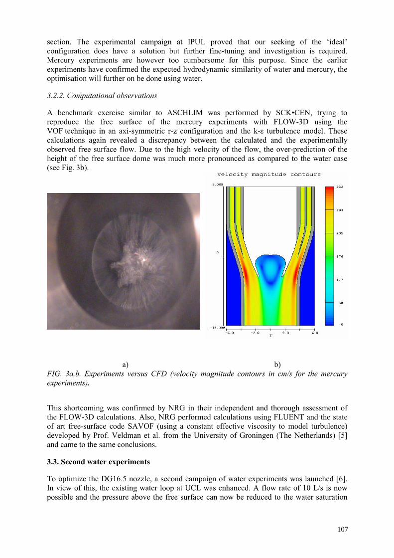
section. The experimental campaign at IPUL proved that our seeking of the ‘ideal’ configuration does have a solution but further fine-tuning and investigation is required. Mercury experiments are however too cumbersome for this purpose. Since the earlier experiments have confirmed the expected hydrodynamic similarity of water and mercury, the optimisation will further on be done using water.

3.2.2. Computational observations

A benchmark exercise similar to ASCHLIM was performed by SCK•CEN, trying to reproduce the free surface of the mercury experiments with FLOW-3D using the VOF technique in an axi-symmetric r-z configuration and the k-ε turbulence model. These calculations again revealed a discrepancy between the calculated and the experimentally observed free surface flow. Due to the high velocity of the flow, the over-prediction of the height of the free surface dome was much more pronounced as compared to the water case (see Fig. 3b).

a) b) FIG. 3a,b. Experiments versus CFD (velocity magnitude contours in cm/s for the mercury experiments).

This shortcoming was confirmed by NRG in their independent and thorough assessment of the FLOW-3D calculations. Also, NRG performed calculations using FLUENT and the state of art free-surface code SAVOF (using a constant effective viscosity to model turbulence) developed by Prof. Veldman et al. from the University of Groningen (The Netherlands) [5] and came to the same conclusions.

3.3. Second water experiments

To optimize the DG16.5 nozzle, a second campaign of water experiments was launched [6]. In view of this, the existing water loop at UCL was enhanced. A flow rate of 10 L/s is now possible and the pressure above the free surface can now be reduced to the water saturation

107

pressure of ca 20 mbar absolute. To be able to investigate the effects of various modifications, the nozzles are made exchangeable, with a high dimensional accuracy to avoid asymmetry and with a drag-limited inlet flow. A Plexiglas measurement section is present for optical analysis and cavitation detection.

A first similarity check showed the same results for the successful DG16.5 nozzle of the mercury experiments with the same features provided boiling of the water is avoided by raising the vacuum pressure up to around 22 mbar. The experimental set up and the obtained free surface are shown in Fig. 4a-c.

4a) 4b)

4c)

FIG. 4a-c. The DG16.5 nozzle and corresponding free surface in the second water experiments.

108

The optimisation process in water is still going on. The feeder section is redesigned. Also, the effects of a limited peripheral swirl flow are investigated. First experiments show that this kind of swirl clearly has a positive effect on the stability in the re-circulation zone.

In view of the benchmarking of CFD codes, elaborate measurement campaigns for velocity and turbulence field determination using Particle Image, LASER Doppler and Ultrasonic Doppler Velocimetry are foreseen. Only the latter technique can be used in the final experiments using the opaque LBE. The setup of the equipment is now under design.

3.4. Future experiments

As the spallation target design is a crucial point for the MYRRHA project, final confirmation experiments are foreseen to be performed with the LBE at similar temperatures.

In view of this, collaboration with Forschungszentrum Karlsruhe (FZK, Germany) has been negotiated and the technical interface has been agreed, aiming at inserting a to-scale model of the MYRRHA spallation target similar to the one in the Mercury loop in their KALLA-THEADES Pb-Bi loop. This Pb-Bi loop is in size similar to the mercury loop but in complexity closer to the MYRRHA spallation loop: it has two free surface levels and a mechanical impeller pump at nominal flow rate. These experiments may ultimately yield also data on loop control parameters and corrosion-like phenomena.

A second campaign of Pb-Bi loop experiments is foreseen to be performed in the CHEOPE loop in collaboration with ENEA (Bologna/Brasimone, Italy). A to-scale model of the MYRRHA spallation target will be inserted in the existing CHEOPE experimental vessel together with a MHD pump, a configuration that will correspond to the minimum closed loop configuration of a MYRRHA like spallation circuit with no detraction by other loop problems. Some experience yield on the dynamics of a magneto hydrodynamic pump is also expected from this experiment.

3.5. Future calculations

To reduce today’s discrepancy between experimental observations and CFD, a research project has been established to widen the model options to full 3-D with an adequate free surface model (VOF with interface reconstruction) and an adequate turbulence treatment (LES to capture the granular structure) and tune these by experimental evidence.

Preliminary calculations by NRG using the 3-D version of the SAVOF code, COMFLO [7], have shown promising results. Therefore, the capabilities of COMFLO will be further explored. One of the possible routes for future calculations could be the implementation of an LES turbulence model in COMFLO. Also a more recent version of FLOW-3D is considered for the tuning.

With a reasonable match of the self-consistent code data and the experimental values in the non-heated case, we will have a good chance of realistic heating results by the code producing the temperature field. From these we can then judge the fulfilment of our design criteria.

4. CONCLUSIONS

The challenge in the MYRRHA spallation target design is to create a heavy liquid metal flow pattern with a free surface within the geometrical constraints imposed by the sub-critical core, adequate to remove the heat deposited by the proton beam so that the vacuum requirements of the beam transport system are met.

109

A series of promising experiments have shown – in principle – the possibility of creation of an adequate flow pattern. Further experimental optimisation of the target nozzle in water is currently going on. Confirmation experiments with lead-bismuth eutectic are planned.

The investigations, however, have also revealed a discrepancy between the experimental pattern and the one calculated with Computational Fluid Dynamics codes. These calculations are indispensable since proton beam heating cannot yet be simulated experimentally because of the lack of a suitable accelerator and neutron compatible experimental environment. Therefore, next to the experimental optimisation of the nozzle, the current research at SCK•CEN aims at reducing the discrepancy between code and experiment by widening the model options in the CFD codes and adapting them by experimental evidence.

So far, there is no evidence that the ‘windowless’ design cannot be made to work and there is a solid optimism that the remaining issues can be resolved. In summary, the results of our design activities, although not yet totally conclusive, look very encouraging to yield the desired target configuration.

REFERENCES

[1] AÏT ABDERRAHIM, H., KUPSCHUS, P., MYRRHA, A Multipurpose Accelerator Driven System (ADS) for Research & Development, March 2002 Pre-Design Report, R-3595, SCK•CEN, Mol, Belgium (2002).

[2] SEYNHAEVE, J.-M., MYRRHA project: R&D Collaboration between SCK•CEN and UCL/TERM: Phase 3, Université Catholique de Louvain, Louvain-la-Neuve, Belgium (2000).

[3] ARIEN, B., ASCHLIM: a 5th FP Project for the Assessment of CFD Codes applied to Heavy Liquid Metals, Proceedings of the International Workshop on P&T and ADS Development, SCK•CEN, BLG-959, ISBN 9076971072, Mol, Belgium (2003).

[4] VAN TICHELEN, K., KUPSCHUS, P., ARIEN, B., AÏT ABDERRAHIM, H., Design and Verification Experiments for the Windowless Spallation Target of the ADS Prototype MYRRHA, Third International Workshop on Utilisation and Reliability of High Power Proton Accelerators, Santa Fe, New Mexico, USA, 2002, OECD/NEA, NEA#04310, ISBN 9264102116 (2003).

[5] SAVOF96 version 2.09 User Manual (Dutch), RUG Groningen (2001). [6] SEYNHAEVE, J.-M., MYRRHA project: R&D Collaboration between SCK•CEN

and UCL/TERM: Phase 4, Université Catholique de Louvain, Louvain-la-Neuve, Belgium (2002).

[7] GERRITS, J., Dynamics of Liquid-Filled Spacecraft, PhD Dissertation, Rijksuniversiteit Groningen, Groningen, Netherlands (2001).

110

THERMOHYDRAULIC BEHAVIOR IN AN ADS TARGET MODEL

A. PEÑA, G.A. ESTEBAN, J. SANCHO

Abstract

The window model of the Accelerator Driven System (ADS) target TS-1, under development in the State Scientific Center of Russian Federation Institute of Physics and Power Engineering (SSC RF IPPE) and Joint Design Burear “Gidropress” for accelerator LANSCE in Los Alamos National Laboratory, serves as model for the calculations done with the FLUENT CFD code presented in this paper. The experimental device represents a tube-to-tube structure. Sodium-potassium (NaK) coolant enters through the inlet connection, and then it flows in the annular channel of the model between tubes towards the membrane positioned at the end of the annular channel. Here, in the form of coming together streams the coolant runs to the center of the membrane, then it turns striking against the membrane surface and passes through the distributing grid. This paper shows calculations and conclusions of the numerical simulation of the ADS target model, from a work that began with a benchmark problem presented at the “10th International meetings of the working group on advanced nuclear reactors thermo hydraulics” in Obninsk, Russia in 2001.

1. INTRODUCTION

Following the benchmark problem presented at the “10th International meetings of the working group on advanced nuclear reactors thermo hydraulics” that took place in Obninsk, Russia, in 2001, a two year project was accepted by the University of the Basque Country in order to correctly finish the former calculations.

Previous preliminary results using the CFD (Computational Fluid Dynamics) codes STAR-CD and FLUENT were presented in the “7th international meeting on partitioning and transmutation” in Jeju, Korea, in 2002. Different mesh configurations and turbulence models were used in the calculations, but one aspect was not taken into account: the proper simulation of the distribution grid, because it was treated as a porous media, instead of drawing the holes. These were substituted by the head losses that they introduce in the flow through the distribution grid. A final effort with this ADS target model has been done with the complete grid geometry of the TS-1, although only half of the device has been represented due to an unreasonable computational effort with the whole geometry. These calculations have been done with the FLUENT V6.0 CFD code.

Important conclusions can be taken for these calculations. One of them is that using the porous media model, the temperature field is fairly enough well foreseen, although the velocity distribution is not properly calculated. Including the distribution grid, this velocity distribution is much more proper.

2. EXPERIMENT DESCRIPTION

The experimental device represents a tube-to-tube structure (Fig. 1). The Sodium-potassium eutectic (NaK) coolant enters through the inlet connection ∅ 68, at a variable temperature from 33 to 37.2°C, and then it flows in the annular channel of the model between tubes ∅ 185 and ∅ 136 toward to the membrane positioned at the end of the annular channel. Here, in the form of coming together streams the coolant runs to the center of the membrane, then it turns striking against the membrane surface and passes through the distributing grid (Fig. 2).

111

Universidad del País Vasco/Euskal Herriko Unibertsitatea, s/n Bilbao, Spain

1 - copper unit with nickel-chrom-heaters 2 - membrane of the target 3 - grid with profiling holes 4 - thermocouple block

FIG. 1. Experimental device.

FIG. 2. Distribution grid.

The coolant flow rate is Q = 7 m3/h. A copper block, simulating the energy deposited by a proton beam interacting with the target, heats the membrane. The heat flux at the membrane being q = 8.6 × 105 W/m2. In order to get an ax symmetric flow in the membrane, a sickle-shaped plate is installed in the upper part of the annular channel [1].

The temperatures are measured in several points of the device, by a mobile chrome-copper thermocouple (Fig. 3).

Outlet Inlet

112

FIG. 3. Mobile thermocouple.

The objective of the benchmark exercise is the comparison of the coolant and membrane temperature at different positions, analyzing the temperature behavior of liquid metal coolant and membrane of the target system, and examining the reliability of the thermal-hydraulics codes and their physical models.

3. NUMERICAL SIMULATION: GEOMETRY AND PHYSICAL MODELS

The geometry for the numerical simulation of the TS1 window model is the one shown in Fig. 4.

FIG. 4. FLUENT meshing of the TS-1 target model.

113

The meshing consists in 228 303 mixed cells. The inner tube cells are hexahedral, while the rest of them are tetrahedral or pyramidal. The computer in which the problem has been run, is a workstation with Microsoft windows 2000, 450 Mhz, and 216 MB of RAM memory. Half of the model has been modelled, and a symmetry boundary condition input in the longitudinal plane. The model is in principle, a symmetric device, in a horizontal plane, but the thermocouple measurements show that this assumption is not a good one. Anyways, due to the capacity of the computer no more complete geometry could be achieved. The turbulence model used for the calculations is the RNG k-ε, with the standard wall functions. Some validations were made with the Reynolds stress model showing better results, but not much difference was made, and the time for running the calculation was very high. Therefore, it was not worthy using them in the new calculations (see Fig. 5).

FIG. 5. Comparison between RSM and RNG k-ε.

These validations were done in the previous calculations, with the porous media model simulating the distribution grid. The discretization schemes in these calculations were QUICK for momentum and energy, and second order UPWIND for turbulence kinetic energy, and dissipation of the turbulence kinetic energy. The material properties for the NaK are shown in Table 1 [1].

TABLE 1. Na-K PROPERTIES

Property Relationship Units

Density T⋅−= 27.01.880ρ kg/m3

Heat capacity 2002.042.092.974 TTc p ⋅+⋅−= )/( KkgJ ⋅

Heat conductivity 200156.00088.0368.22 TT ⋅+⋅−=λ )( KmW ⋅

Dynamic viscosity 62 10)0094.02497.4162.807( −⋅⋅+⋅−= TTμ sPa ⋅

The boundary condition for the external walls is adiabatic, and the cooper block of the experiment has been simulated by a heat flux through the membrane wall.

Fluid temperature s=1

0

50

100

150

200

250

0 5 10 15 20

thermocouple number

tem

pera

ture

(ºC

)

FLUENT(RSM) FLUENT(RNG)

114

4. NUMERICAL SIMULATION: RESULTS

Using the thermocouple measurements, the results obtained with FLUENT were compared with them to validate the physical models of the code. Comparing the experimental measurements, with the computational ones, it can be observed that in the hotter part of the device (near the membrane), the results are worse than in the rest of it (see Fig. 6).

FIG. 6. FLUENT calculation versus experimental measurements.

Thermocouples s=1mm

30405060708090

100110120

0 5 10 15 20

Thermocouple

Tem

pera

ture

(ºC

)

ExperimentFLUENT

Thermocouples s=3mm

30405060708090

100110120

0 5 10 15 20

Thermocouple

Tem

pera

ture

(ºC

)

ExperimentFLUENT

Thermocouples s=10mm

30.0

40.0

50.0

60.0

70.0

80.0

90.0

0 5 10 15 20

Thermocouple

Tem

pera

ture

(ºC

)

ExperimentFLUENT

Thermocouples s=5mm

3040

506070

8090

100

110120

0 5 10 15 20

Thermocouple

Tem

pera

ture

(ºC

)

ExperimentFLUENT

Thermocouples s=60mm

30,0

35,0

40,0

45,0

50,0

55,0

60,0

0 5 10 15 20

Thermocouple

Tem

pera

ture

(ºC

)

Experiment

FLUENT

Thermocouples s=200mm

30,0

32,0

34,0

36,0

38,0

40,0

42,0

44,0

0 5 10 15 20

Thermocouple

Tem

pera

ture

(ºC

)

ExperimentFLUENT

115

The graphics represent the temperature of each thermocouple pitch, whose numbers can be seen in Fig. 3. From positions s = 1 to 5 mm (taken from the membrane), the temperature gradient along the longitudinal direction, in the 6th thermocouple position measurement is very high in the experimental device, compared with the FLUENT calculation. The observed temperature difference in the colder measurements are due to the fact that the computational calculations have been made with constant inlet temperature, while the experimental device suffered pulsations of temperature [1].

Velocity vectors in Figs 7 and 8 show that some recirculation is present after the distribution grid, and that there is a stagnant point in the middle of the membrane. The supposed horizontal symmetry in the computational simulation is not so, as the thermocouples and the previous calculations showed [2]. Therefore, the calculated temperatures in the calculation are not correct, although, in principle, the device seems to be symmetric.

The code is not able not reproduce properly the temperature field. It underestimates the heat transfer to the liquid metal from the membrane. One solution should be a change of the turbulence Prandtl number. The relation between turbulence heat and momentum transfer (indicated by the turbulence Prandtl number) is different in liquid metals compared with more usual fluids as water or air, and this experimental coefficient included in the codes, has been deduced, mainly, through experiments with water and air. A change in the turbulence Prandtl number leads to a change in the results [3], but this not the best model to prove this. Complexity in experimental measurements, as well as modelling of the distribution grid in the CFD code, does not allow doing many validation studies. Another point is the simulation of the boundary layer. This geometry was very complicated, and was not possible to use a very fine mesh in the wall. In the simulation there is an y + < 130.

Using the porous media model for the distribution grid seems to be a very helpful tool. Temperatures are a little bit higher, and the velocity field is not managed, but the need of less number of cells allows an easier study of the turbulence models, the grid independence, with this model [2].

FIG. 7. Velocity vectors near the membrane.

116

FIG. 8. Velocity vectors showing the recirculation after the distribution grid.

5. CONCLUSIONS AND SUMMARY

Since the benchmark was proposed, the simulation has been improved, by increasing the number of cells and by correctly drawing the distribution grid. This last modelling has improved the velocity field, and therefore the temperature one, but in this case, the temperature near the membrane is not good. It is well known that grid independence must be reached, and these results are an example of it. Due to computational limits, this is not an easy parameter to achieve. Commercial codes are worse prepared for working with liquids metals than with more usual fluids as water and air. Some validations must be done with the turbulence Prandtl number, in order to achieve a good coefficient for liquid metals. The thermal boundary layer modelling is another critical point that differs from code to code [2]. Porous media model is a good tool for managing quick calculations, above all with the new version of FLUENT that is able to calculate the superficial velocities corresponding to the ones of the fluid, flowing inside the holes or the tubes.

REFERENCES

[1] ORLOV, YU, et al., Specification of the Benchmark Problem. Thermal Experiments in the ADS Target Model, paper presented in the 10th International Meeting on the IAHR Working Group on the Advanced Nuclear Reactors Thermal Hydraulics, 17–19 July 2001, IPPE, Obninsk, Russian Federation.

[2] PEÑA, A., ABÁNADES, A., ESTEBAN, G.A., LEGARDA, F., SANCHO, J., Activities of UPV/EHU concerning the TS-1 Target System Experiments, paper presented in the 7th Information Meeting in Partitioning and Transmutation, 14–16 October 2002, Jeju, Republic of Korea.

[3] BUONO, S., MACIOCCO, L., MOREAU, V., SORRENTINO, L., CFD Simulation of Heated Round Jet of Sodium (TEFLU Benchmark), CRS4 Technical Report 00-86 (July 2001).

117

DEVELOPMENT AND APPLICATION OF CFD CODES MASKA-LM AND PORT 3D FOR INVESTIGATION OF THERMAL HYDRAULICS OF LEAD COOLED FAST REACTOR BREST

A.A. VEREMEEV, V.YA. KUMAYEV, A.A. LEBEZOV State Scientific Center, Institute of Physics and Power Engineering (SSC RF-IPPE), Obninsk, Russian Federation

Abstract

The report is devoted to the development and application of the two-dimensional MASKA-LM and three-dimensional PORT 3D computer codes intended for numerical calculations of lead coolant flows, temperatures and transport of impurities in reactors with integral design of BREST type. The set of governing equations to be solved is based on the porous body model and describes the thermal-hydraulic processes in the reactor as a whole. The numerical method for solution of the governing equations is discussed. Examples of calculation of the coolant flows, temperatures and impurities transport in the primary circuit of the BREST are presented. The three-dimensional calculations were performed using fine numerical grids consisting of more than 20 million computational cells. The numerical grid covered the whole primary circuit of the integral reactor, including the core, steam generators and pumps.

1. JOINT SIMULATION OF THERMAL-HYDRAULIC AND MASS TRANSFER PROCESSES BY MASKA-LM CODE

The description of heat and mass transfer in liquid metal systems, proceeding in the coolant and at the interface “coolant – structural materials”, is a complex problem involving the joint simulation of thermal-hydraulic, physical and chemical processes in view of the real configuration of the reactor circuit. The paper presents the state-of-the-art in the development of two-dimensional code MASKA-LM [1–3] and the results of trial calculations of heat and mass transfer in the primary circuit of the lead cooled reactor.

The chemical reaction rate constants, the values of saturation concentrations of impurities, which are known approximately so far, have a significant influence on the results of calculations of the processes under consideration. Therefore in calculations the specified values of constants were taken from the rated range of their possible values, and the results of calculations should be considered tentative and intended to estimate and check the workability of the technique and code.

1.1. Mathematical model

Processes of convective mass transfer are determined by spatial and non-stationary flow and heat exchange of coolant. A two-dimensional model of mass transfer in porous body approach has been developed at present, allowing one to simulate the global distribution of mass flows of impurities. Further extension of the developed approach on the general three-dimensional case is supposed.

Global mass transfer in the circulating loop is described by a set of non-stationary differential equations of convective-diffusive transfer of multicomponent impurity with sources and sinks. The equation of transfer in the Cartesian coordinates reads:

k

nn

k

N

p

np

k

knn

x

CD

xJ

x

uCC

∂

∂

∂

∂=−

∂

∂+

∂

∂∑=

εεε

τ

ε

1 (1)

119

Where: ku - components of velocity vector; nc - concentration of impurity component n; nD - diffusivity factor of component n in the coolant; ε - volumetric porosity of medium.

Porosity of medium is a spatially dependent function that varies in time due to deposition of solid phase of impurity on the surfaces of the loop. The mass source npJ can be represented as volumetric source np

vJ and surface source npsJ .

The momentum equation of coolant in porous medium, which models the structure and geometry of the loop element under consideration, and the continuity equation read:

−∂

∂

∂

∂+

∂

∂−=

∂

∂+

∂

∂

k

i

kiok

ik

i

x

u

xx

p

x

uu

uεν

ε

1

ρ

1

τ

( )o

iiiT

guud ρ

ρ

2

1

г+Λ (2)

0ε=

∂

∂

k

k

x

u (3)

Where: ρ - density; p - pressure; ν - kinematics viscosity; Λ - resistance factor of the porous medium; гd - hydraulic diameter.

The energy equations for coolant and porous body are:

( )SttKqx

t

xx

tuctcsv

kkk

kpp−++

∂

∂

∂

∂=

∂

∂+

∂

∂εελ

ερ

τ

ερ (4)

( )SttKqx

t

x

tcsvss

k

sss

k

spsss−−+

∂

∂

∂

∂=

∂

∂ελε

τ

ρε (5)

Where: t - coolant temperature; st - porous body temperature; ε1ε −=s - volumetric fraction of porous body (solid bodies) in the medium; sρ , ρ - density of coolant and porous body;

psp cc , - specific heat capacity of coolant and porous body; sλ , λ - conductivity of coolant and porous body; vsv qq , - volumetric density of heat generation in coolant and porous body; S - surface of heat exchange between coolant and porous body in unit medium; K - heat transfer coefficient between coolant and porous body.

The equations for determination of the sources of the impurities of iron, magnetite, and oxygen are as:

⎟⎟

⎠

⎞

⎜⎜

⎝

⎛ −=

ov A

CCCJ 4O3Fe

4PbO

3Fe

(6)

г

PbOPbOPbO χ44

d

CCAJJ w

v

−+−=

(7)

120

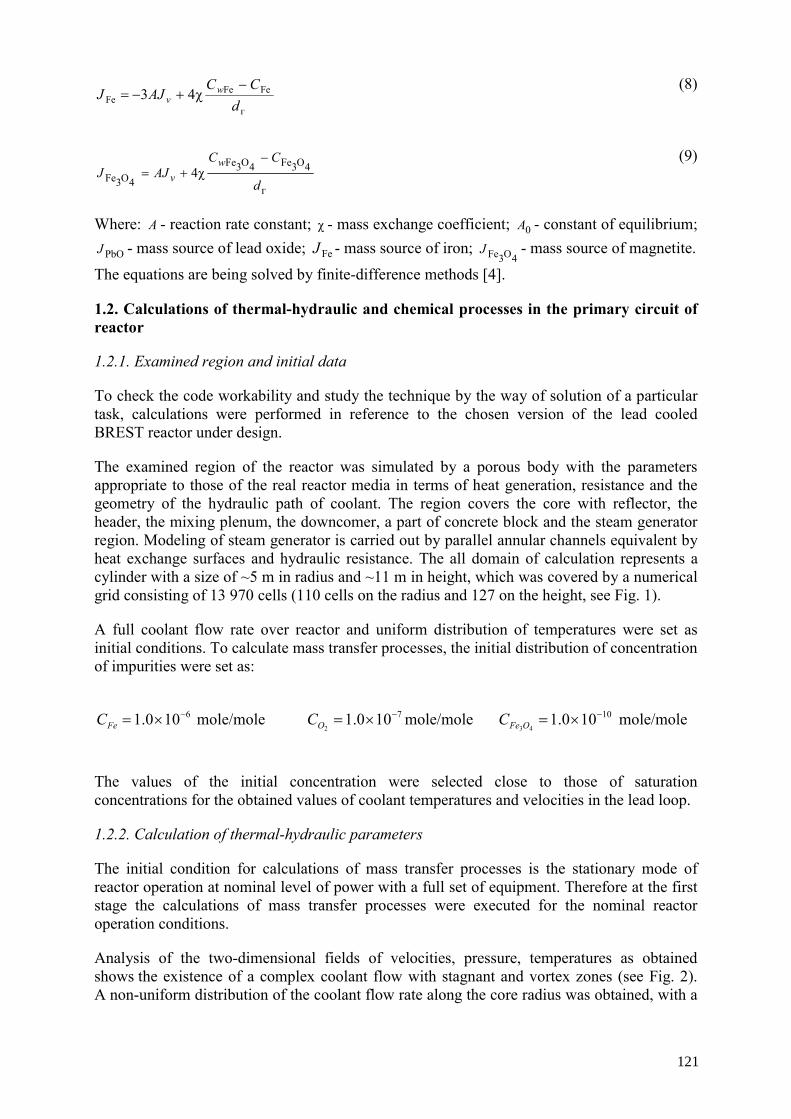
г

FeFeFe χ43

dCC

AJJ wv

−+−= (8)

г

4O3Fe4O3Fe

4O3Fe χ4d

CCAJJ

wv

−+=

(9)

Where: A - reaction rate constant; χ - mass exchange coefficient; 0A - constant of equilibrium;

PbOJ - mass source of lead oxide; FeJ - mass source of iron; 4O3FeJ - mass source of magnetite.

The equations are being solved by finite-difference methods [4].

1.2. Calculations of thermal-hydraulic and chemical processes in the primary circuit of reactor

1.2.1. Examined region and initial data

To check the code workability and study the technique by the way of solution of a particular task, calculations were performed in reference to the chosen version of the lead cooled BREST reactor under design.

The examined region of the reactor was simulated by a porous body with the parameters appropriate to those of the real reactor media in terms of heat generation, resistance and the geometry of the hydraulic path of coolant. The region covers the core with reflector, the header, the mixing plenum, the downcomer, a part of concrete block and the steam generator region. Modeling of steam generator is carried out by parallel annular channels equivalent by heat exchange surfaces and hydraulic resistance. The all domain of calculation represents a cylinder with a size of ~5 m in radius and ~11 m in height, which was covered by a numerical grid consisting of 13 970 cells (110 cells on the radius and 127 on the height, see Fig. 1).

A full coolant flow rate over reactor and uniform distribution of temperatures were set as initial conditions. To calculate mass transfer processes, the initial distribution of concentration of impurities were set as:

6100.1 −×=FeC mole/mole 7100.12

−×=OC mole/mole

10100.143

−×=OFeC mole/mole

The values of the initial concentration were selected close to those of saturation concentrations for the obtained values of coolant temperatures and velocities in the lead loop.

1.2.2. Calculation of thermal-hydraulic parameters

The initial condition for calculations of mass transfer processes is the stationary mode of reactor operation at nominal level of power with a full set of equipment. Therefore at the first stage the calculations of mass transfer processes were executed for the nominal reactor operation conditions.

Analysis of the two-dimensional fields of velocities, pressure, temperatures as obtained shows the existence of a complex coolant flow with stagnant and vortex zones (see Fig. 2). A non-uniform distribution of the coolant flow rate along the core radius was obtained, with a

121

non-uniformity span at its outlet of ~9% of the average velocity. In particular, the presence of non-uniform velocity profile was detected at the core inlet, which influenced the increase of non-uniform coolant heating over profiling zones. The coolant flow rate through the core was ~91.3%. The coolant flow rate through lateral reflector equaled ~7.2% and through inner storage of fuel ~1.5% of the total flow rate.

The average coolant temperature at the core outlet was by ~20°C higher than the average temperature at the reactor outlet. The non-uniformity of coolant temperature distribution that was obtained along the outlet pipe diameter amounted to 55°C. The evaluation of the external surface of fuel pin claddings revealed that the maximum temperature is achieved in the central part of the core.

0 1 2 3 4 5

Радиус, м

0

1

2

3

4

5

6

7

8

9

10

11

Высота

, м

1

3

2

2

4

5

6

7

8

0 1 2 3 4 5

Радиус, м

0

1

2

3

4

5

6

7

8

9

10

11

Высота

, м

1 – core 2 – face reflector 3 – lateral reflector 4 – inner storage of spent fuel subassemblies 5 – lower plenum 6 – upper plenum 7 – downcomer 8 – steam generation

FIG. 1. Examined region for reactor modeling. FIG. 2. Coolant velocity field.

Hei

ght,

m

Hei

ght,

m

Radius, m Radius, m

122

1.2.3. Calculations of impurity mass transfer processes

Calculations were performed of the impurity transport of iron, oxygen and magnetite in the primary reactor circuit. At the initial moment, a uniform distribution of concentration of impurities was set over the whole examined region, with a steady-state field of coolant velocity and temperature. For subsequent moments, propagation of impurities over the reactor due to transport of coolant by flow and diffusion was evaluated, with the chemical interaction of impurities between each other considered. In the given statement of the problem, possible formation of solid particles of impurities was not taken into account. In Fig. 3, the distribution of concentration of iron dissolved in lead coolant is shown. In Fig. 4, the distribution of concentration of oxygen dissolved in lead coolant is given.

0 1 2 3 4 5

Радиус, м

0

1

2

3

4

5

6

7

8

9

10

11

Высота

, м

0 1 2 3 4 5

Радиус, м

0

1

2

3

4

5

6

7

8

9

10

11

Высота

, м

FIG. 3. Distribution of iron concentration, FeC mole/mole.

FIG. 4. Distribution of oxygen concentration,

2OC mole/mole.

The duration of the calculated process of impurity mass transfer in reactor loop was 10 hours. For this time, a quasi-stationary distribution of impurity concentration has been established. The established distribution is not uniform in this case because of the permanent action of impurity sources and sinks. With long-time consideration of mass transport process, the concentration profile will not undergo essential variations; however, the average concentration values will vary slowly due to the effect of the physical and chemical processes proceeding in the coolant. The maximal concentrations obtained in trial calculations for oxygen 1010OC −= mole/mole and iron 610FeC −= mole/mole are observed in the zone with maximum temperature (the top part of the core and the upper plenum), the minimal concentrations - in stagnant zones 1310OC −= mole/mole and 710FeC −= mole/mole.

Hei

ght,

m

Hei

ght,

m

Radius, m Radius, m

123

2. CALCULATION INVESTIGATIONS OF THREE-DIMENSIONAL THERMO-HYDRAULICS OF LEAD COOLANT OF FAST REACTOR

2.1. Specific features of PORT 3D code

For calculation of the three-dimensional single-phase coolant flow and the temperature fields in the primary circuit of the reactor with integral design, the PORT 3D code has been developed at SSC RF IPPE [5, 6]. To describe the global hydrodynamics and heat exchange, a generalized porous body model was used, which allows a combined simulation of processes in the core, in the regions containing lattices, fuel bundles as well as in chambers and cavities with complicated geometry. The solution of the equations of hydrodynamics and energy is carried out by the finite-differences method by using a triangular-prismatic grid of a large number of cells [7, 8] (see Fig. 5). The bases of cells (of triangular-prisms) are in the planes parallel to plane XY. The sizes of the cells of the computation grid were chosen as small as possible and were restricted from bottom by the available computer memory. In the present calculations, the lengths of cells sides were 50 mm in plane XY and 100 mm along the Z axis.

u u u

u

u u

u u

u u u u

u u u u

v

v

v

v

v

v v

v

u

u

u

u

u

u

w

w

XZ

X Y

X

Y

1 2 3 4 5 6 7 8 9

1 3 5 7 9 11 15 17 1913 21

w

w

i

j

S

M

M

M

X

YZ

A. Grid and cell indexing in XY plane

B. Grid fragment in

XZ plane

C. Grid fragment in XY plane D. Three-dimensional view of grid cells

FIG. 5. Triangular-prismatic grid and variable localization.

124

To specify the examined region simulating the reactor as a system of structures with given properties, a text interface of code was developed. A typical scheme of specifying the examined region and the types of modeled structures of the object are given below.

A BC

Initial object Allocation of typical structures

Allocation of elementary bodies

Synthesis of object model: 1. Modelling elementary bodies using calculation grid; 2. Modelling typical structures; 3. Selective combining elementary bodies; 4. Automatic connection of structure functions.

ε porosity; dг hydraulic diameter; kф form factor; s pitch of rods; d rod diameter; Nр number of spacer ribs; Y height of ribs; X thickness of ribs; H the period winding; λk resistance factors; αk heat transfer coefficient; P thermophysical properties

Types of modeled structures Determining parameters of model

1. Modelling elementary bodies on a grid – – – – – – – – P

2. Continuous impenetrable bodies – – – – – – – – P

3. Systems of parallel isolated channels ε dг kф – – – – – P

4. Bundles of rods with triangular arrangement – – s d Nр Y X H P

5. Bundles of rods with square arrangement – – s d Nр Y X H P

6. Abstract porous bodies of other structure ε λ1 λ2 λ3 α1 α2 α3 – P

125

2.2. Use of PORT3D code for researches of the three-dimensional thermohydraulics of a reactor with integrated configuration

Improvement of the technology of using the PORT 3D code for numerical studies of the three-dimensional fields of coolant velocities and temperatures was exemplified by calculating of the full closed primary circuit of one of intermediate variant of BREST reactor with integral design. The calculation model represents a ½ part of reactor, separated by a vertical plane of symmetry (see Fig. 6).

V1 V2

V3

2

3 1

4

V4

Plane of symmetry

Y

X

(r, ϕ)

Switched-off loop

modules of steam generators and pumps

FIG. 6. The examined model of reactor in plane XY.

Two modes of reactor operation are examined: the nominal one at a level of 100% power and a mode of operation with one switched-off loop. The purpose of work is to produce three-dimensional distributions of coolant velocities and temperatures in the core, the upper plenum with outlet pipes, in the primary circuit as a whole. The results of calculations can be used in designing reactor components.

The nominal mode of operation is considered as a base mode for which the design values of all basic thermal and hydraulic characteristics of reactor components are known. The accuracy of numerical calculations of the thermal hydraulic characteristics is checked just against this mode of operation. In the nominal mode of operation, four loops of the reactor work symmetrically. Therefore with reference to heat and mass transfer processes in the core and upper plenum, the results of calculations for the full model practically do not differ from the results of pre-computations in which blocks of pumps and steam generators were not considered.

126

In the full model of the primary circuit, the flow rate of coolant is predetermined only in pumps. In branches of the flowing path of the primary circuit the flow rate is established in the course of solving the hydrodynamics problem and depends on hydraulic resistances and flow patterns in all set of branches. With a given flow rate through pumps, the deviation from the required design values of flow rates (owing to calculation uncertainly) can take place only in the parallel branches of the hydraulic path. At symmetric work of loops, the deviation takes place only in parallel branches not identical in design. Distribution of heat sink in steam generator was set to simulate heat exchange between the primary and secondary circuits.

In operation conditions with one switched-off loop, the flow rate through the core varies due to the action of the following major factors:

− Switching-off one pump results in general reduction of flow rates in the primary circuit; − Bypass of the coolant through pumps connection collector reduces the share of flow rate

through the core; − Variation of free levels results in increase of the flow rate of working pumps and

compensates in part the reduction of the flow rate through the core.

In numerical calculations reactor power was reduced proportionally to the flow rate through the core, and the total sink of heat in steam generators was equal to the aggregate power generation.

As a result of calculations it was found, that the values of flow rate in various branches of the flowing path of the primary circuit are different for the nominal mode of operation and a mode of operation with the switched-off loop. However, this difference is rather insignificant. In Figs 7–10, velocity and temperature fields in the most typical sections of the reactor are shown for the switched-off loop operation mode.

Coolant passes to the lower plenum over the annular downcomer from the loop pressure head level as well as over connecting pipes from the bottom past of pump – steam generator modules. The coolant passes the core up to the top of the upper plenum. In this section of the flow path the coolant flow and the temperature distribution are like those in the nominal operation condition at 100% power. An annular zone of recirculation flow is formed in the periphery of the lower part of the upper plenum. A part of coolant is taken off from the periphery of the upper plenum and comes directly to the pump – steam generator modules and from these to the pump inlet.

As in the nominal mode of operation, the flow in the upper plenum is stratified in temperature. The stream of the hottest coolant from the core moves upwards in the central part of the plenum, rises up to the top level and enters the outlet pipes in their top part. Streams of the least heated coolant from reflectors and fuel store rise upwards and go out in to the outlet pipes in their bottom part.

Temperature distributions in over the inlet sections of the outlet pipes are shown in Fig. 11. It is seen, that the average and the maximal values of temperature at the entrance of the outlet pipes of working loops 2 and 3 almost coincide, whereas the minimal ones considerably differ. The hot layers of coolant are pushed aside from the entrance section of the outlet pipe of the switched – off loop 1, therefore the temperature drop in this section is insignificant.

127

-10

-9-8

-7-6

-5-4

-3-2

-10

12

34

56

78

910

м

2 м

/с

FIG

. 7. M

ode

of o

pera

tion

with

switc

hed-

off l

oop.

Vel

ocity

fiel

d in

XZ

plan

e.

128

-10

-9-8

-7-6

-5-4

-3-2

-10

12

34

56

78

910

м

FIG

. 8. M

ode

of o

pera

tion

with

switc

hed-

off l

oop.

Vel

ocity

fiel

d at

the

mid

dle

leve

l of o

utle

t pip

es o

f rea

ctor

.

129

-10

-9-8

-7-6

-5-4

-3-2

-10

12

34

56

78

910

м

FI

G. 9

. Mod

e of

ope

ratio

n w

ith sw

itche

d-of

f loo

p. T

empe

ratu

re fi

eld

in X

Z pl

ane.

130

-10

-9-8

-7-6

-5-4

-3-2

-10

12

34

56

78

910

м

FIG

. 10.

Mod

e of

ope

ratio

n w

ith sw

itche

d-of

f loo

p. T

empe

ratu

re fi

eld

at th

e m

iddl

e le

vel o

f out

let p

ipes

of r

eact

or.

131

Coolant passes to the lower plenum over the annular downcomer from the loop pressure head level as well as over connecting pipes from the bottom past of pump – steam generator modules. The coolant passes the core up to the top of the upper plenum. In this section of the flow path the coolant flow and the temperature distribution are like those in the nominal operation condition at 100% power. An annular zone of re-circulation flow is formed in the periphery of the lower part of the upper plenum. A part of coolant is taken off from the periphery of the upper plenum and comes directly to the pump – steam generator modules and from these to the pump inlet.

As in the nominal mode of operation, the flow in the upper plenum is stratified in temperature. The stream of the hottest coolant from the core moves upwards in the central part of the plenum, rises up to the top level and enters the outlet pipes in their top part. Streams of the least heated coolant from reflectors and fuel store rise upwards and go out in to the outlet pipes in their bottom part.

Temperature distributions in over the inlet sections of the outlet pipes are shown in Fig. 11.

Loop 1Loop 3 Loop 2Loop 3 Loop 2 Loop 1

FIG. 11. Mode of operation with switched-off loop. Temperature distribution at outlet pipes inlet.

It is seen, that the average and the maximal values of temperature at the entrance of the outlet pipes of working loops 2 and 3 almost coincide, whereas the minimal ones considerably differ. The hot layers of coolant are pushed aside from the entrance section of the outlet pipe of the switched – off loop 1, therefore the temperature drop in this section is insignificant.

3. CONCLUSION

The developed code MASKA-LM allows one to calculate the issue of components of structural materials into coolant as impurities, their interaction with oxygen, the formation of a disperse phase, transport of impurity round the circuit in view of the spatial distribution of coolant flows and temperatures.

The calculations as performed using the MASKA-LM code of heat and mass transfer processes over the circuit with lead coolant have shown its workability and qualitative conformity of the results of calculations to the physics of the modeled processes.

132

Using the PORT 3D code, three-dimensional calculations have been performed of coolant flows and temperatures for the primary circuit of BREST reactor. Temperature stratification at the inlet of outlet pipes is determined.

It is shown, that the relative values of flows rates through different branches of the primary circuit differ a little bit for the nominal mode of operation and for the mode of operation with switched-off loop. Distributions of temperature at the entrance of outlet pipes are different and depend on their position relative to the outlet pipe of the switched-off loop. The average and maximal values of temperature at the entrance of the outlet pipes of working loops 2 and 3 almost coincide, whereas minimal ones considerably differ.

REFERENCES

[1] KUMAYEV, V.Y., LEBEZOV, A.A., Numerical Modeling of Hydrodynamics and Heat Transfer in the Primary Circuit of BREST-OD-300 Reactor, Mathematical models for research and substantiation of the characteristics of equipment and reactor as a whole at their creation and operation, Collection of theses of seminar, Sosnoviy Bor, NITI (2000) p. 72.

[2] KUMAYEV, V.Y., et al., Development of Code MASKA-LM for Modelling Heat and Mass Transfer and Corrosion of Steels in Reactors with Liquid Metal Coolant, Thermophysical properties of substances (liquid metals and alloys), Theses of report at International Seminar, Nalchik (2001) p. 57.

[3] KUMAYEV, V.Y., et al., MASKA-LM- a Code for Calculation of Heat and Mass Transfer of Impurity in Liquid Metal Loops, Heat and mass transfer and properties of liquid metals, Proc. Conf., Vol. 1, Obninsk, Russian Federation (2002) p. 295.

[4] PATANKAR, C., Numerical Methods for Solving the Problems of Heat Exchange and Dynamics of Liquid, Energoatomizdat (1984).

[5] VEREMEEV, A.A., Three–dimensional Thermohydraulic Code PORT3D. The Concept and Realization of Objective Model of Anisotropic Porous Body, Preprint IPPE-2852, Obninsk, Russian Federation (2000).

[6] VEREMEEV, A.A., Modelling of Flows and Heat Exchange in Porous Structures and Direct Local Modelling in Thermohydraulic Code PORT3D, Thermophysics-2001, Thermo-hydraulic codes for power reactors, Obninsk, Russian Federation (2001) p. 235.

[7] KUMAYEV, V.Y., LEONCHUK, M.P., Numerical Modeling of Three-dimensional Calculations of Coolant Flows in Rod Bundles, Preprint IPPE-1773, Obninsk, Russian Federation (1985).

[8] KUMAYEV, V.Y., LEONCHUK, M.P., Numerical Modeling of Three-dimensional Coolant Flows in Fuel Rod Bundles, M., J. Atomic Energy, V.60, issue 6 (1986).

133

CFD SIMULATION OF X-ADS DOWNCOMER THERMAL STRATIFICATION

V. ANISSIMOV Ente Nuove Technologie, Energia e Ambiente (ENEA), Bologna, Italy

A. ALEMBERTI Ansaldo Energia S.p.A, Genoa, Italy

Abstract

This work presents a numerical simulation using CFX 4.4 of the Energy Amplifier Experimental Facility (X-ADS) downcomer channel. The simulation is focused on the Steady-State Analysis. The Intermediate Heat exchangers (IHX) of the X-ADS reference configuration are immersed in the lead-bismuth eutectic of the downcomer. Due to the absence of a physical separation between the primary coolant hot and cold collectors, two different flow paths are available in the downcomer region: inside the IHX and outside it (IHX by-pass flow). The amount of IHX by-pass flow is determined by the balance between the driving force due to buoyancy (originated by the weight difference between the cooled fluid inside the IHX and the hot outside downcomer fluid) and the IHX pressure losses. At the IHX exit the two flow paths are mixed before the core inlet. This fact provides a potential for a downcomer thermal stratification, which is influenced by the actual value of coolant flow rate outside the IHX. The amount and extension of the thermal stratification phenomena is the object of this study. The simulation allowed studying the position and intensity of the thermal stratification phenomena. Several runs have been performed. However, to limit the extension of the paper, we deal with the results of only one of the calculations performed, which resulted in the worst condition from the point of view of thermal loads on the structure. Other results obtained will be shortly recalled when needed.

1. THE X-ADS DOWNCOMER SUB-SYSTEM

The simplified scheme of the primary coolant flow paths is shown in Fig. 1.

FIG. 1. Primary coolant flow paths.

135

The IHXs are of the “bayonet” type, with arrays of straight tubes contained within a vertical shell, anchored to an upper support tube sheet. A single bayonet assembly consists of a pair of concentric tubes to allow the inversion of the secondary coolant flow from downward to upward (see Fig. 2).

Fig. 2. Intermediate heat exchanger.

Only one IHX is shown, but there are four IHXs immersed in the primary coolant located in the hot pool annular region between the cylindrical inner vessel and reactor vessel. No solid structure separates the primary coolant hot and cold collectors. The reactor vessel is a cylindrical shell with a hemispherical bottom. The internal structure is not axially symmetrical but has a transversal symmetry plane (see Fig. 3).

136

3a)

CFXCOMPUT.DOMAIN

90°

58°

3b)

Fig. 3a,b. CFX Computational domain.

137

The IHX is enclosed in a 1 cm steel shell, except for the upper 60 cm, which serve as inlet region. The skirt (lower part of the shell) goes 1.4 m deeper than the tubes to enhance the natural circulation driving force.

2. NUMERICAL SIMULATION GENERAL CHARACTERISTICS

The computational domain used for the CFX simulation is evidenced by the outline shown in Fig. 3 on the mechanical drawing cross sections. The simulation involves only about one eighth of the whole downcomer. This approximation has been made due to the limited amount of computational resources (Silicon Graphics OCTANE: RAM, 1 GB; CPU MIPS R12000, 300 MHz), which is a very critical point for this analysis. A symmetry boundary condition has been imposed on the cutting sections. The computational model is presented in details in Fig. 4.

FIG. 4. CFX downcomer model (model isometric view).

138

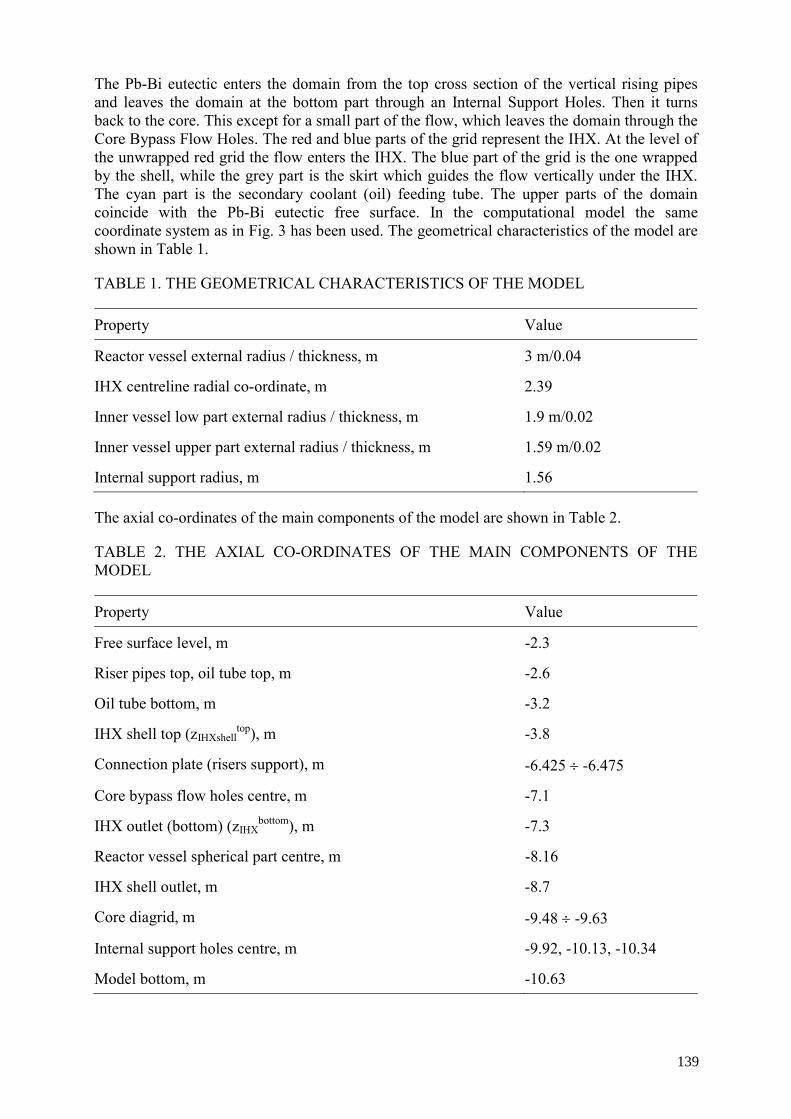
The Pb-Bi eutectic enters the domain from the top cross section of the vertical rising pipes and leaves the domain at the bottom part through an Internal Support Holes. Then it turns back to the core. This except for a small part of the flow, which leaves the domain through the Core Bypass Flow Holes. The red and blue parts of the grid represent the IHX. At the level of the unwrapped red grid the flow enters the IHX. The blue part of the grid is the one wrapped by the shell, while the grey part is the skirt which guides the flow vertically under the IHX. The cyan part is the secondary coolant (oil) feeding tube. The upper parts of the domain coincide with the Pb-Bi eutectic free surface. In the computational model the same coordinate system as in Fig. 3 has been used. The geometrical characteristics of the model are shown in Table 1.

TABLE 1. THE GEOMETRICAL CHARACTERISTICS OF THE MODEL

Property Value

Reactor vessel external radius / thickness, m 3 m/0.04

IHX centreline radial co-ordinate, m 2.39

Inner vessel low part external radius / thickness, m 1.9 m/0.02

Inner vessel upper part external radius / thickness, m 1.59 m/0.02

Internal support radius, m 1.56

The axial co-ordinates of the main components of the model are shown in Table 2.

TABLE 2. THE AXIAL CO-ORDINATES OF THE MAIN COMPONENTS OF THE MODEL

Property Value

Free surface level, m -2.3

Riser pipes top, oil tube top, m -2.6

Oil tube bottom, m -3.2

IHX shell top (zIHXshelltop), m -3.8

Connection plate (risers support), m -6.425 ÷ -6.475

Core bypass flow holes centre, m -7.1

IHX outlet (bottom) (zIHXbottom), m -7.3

Reactor vessel spherical part centre, m -8.16

IHX shell outlet, m -8.7

Core diagrid, m -9.48 ÷ -9.63

Internal support holes centre, m -9.92, -10.13, -10.34

Model bottom, m -10.63

139

The computational domain inlet consists of the outlet of 2 rising pipes. The area of the simulated pipes has been adjusted due to the fact that the riser tubes numbers for each IHX is 6 rising pipes (3 rising pipes for half IHX).

As a consequence the pipes in the computational domain have been transformed into pipes with an ellipsoidal cross section with semiaxis 10 cm×12.61 cm instead of a circular cross section with radius of 10 cm.

The inlet-imposed velocity is about 0.88 m/s, which gives the desirable mass flow rate. This velocity is a slightly higher than the expected mean velocity in the real rising pipes, but it is consistent with a bubbly flow with a void fraction of about 14% at the rising pipes outlets. The regions with bubbly flow rising pipes have not been included in the computational domain to save computer resources. The model includes only external surfaces of the rising pipes.

The inlet turbulent intensity τinlet and the turbulent length linlet must be specified when applying the RNG κ−ε turbulence model. We assigned linlet = 0.2 m, equal to the inner diameter of the riser tubes, and τinlet = 0.037. The inlet temperature of the computational domain is Tinlet = 400 C.

The computational domain outlet consists of three annular slots in the Internal Support. They are representative of the three series of holes in the real geometry.

Pb-Bi eutectic lives the domain also through an annular slot in the Inner Vessel, which represents the Core Bypass Flow Holes in the real geometry. An inlet boundary condition with negative velocity has been used at this boundary.

The appropriate velocity value has been chosen to obtain the design value of the core bypass flow rate. The height of each annular slot is set to the minimum value that allows four cells in the axial direction.

The free surface at the top of the coolant is not simulated precisely. In most runs the free surface was represented by a symmetry plane. This is for a number of reasons ranging from the additional computational cost associated with the free surface simulation to the fact that in reality the riser outlet is characterised by a bubbly flow regime. It has anyway to be pointed out that the effect of the presence of the free surface is expected to be localised in the upper part of the domain and should have a minimum influence on the thermal-hydraulic field in the rest of the domain. In fact, some runs using different free surface models (solid wall or moving free surface in the transient run) produced very similar results, at least in the regions far from free surface.

The Reactor Vessel Spherical Part has been simulated using CFX User Fortran routines, introducing a region with a very high resistance in place of a solid wall (see Fig. 4).

The IHX has been simulated as a porous media. The porosity is constant and is taken directly from the bundle geometrical structure. The relevant IHX characteristics used by the numerical simulation are given in Table 3.

140

TABLE 3. THE IHX CHARACTERISTICS USED BY THE NUMERICAL SIMULATION

Property Value

Outer tube external diameter, d 25.4 mm

Outer tube thickness, t 1.2446 mm

Inner tube external diameter, d1 19.05 mm

Number of tubes, ntubes 1072

Number of rods, nrods 24

Pitch, s 32.5 mm

Roughness of surfaces, Δ 0.05 mm

Hydraulic diameter, dh 20.45 mm

Porosity, α 0.4666

Superficial area 1.041 m2

Height 4.1 m

IHX shell external dimensions 675×1 750×4 900 mm

The porous media resistance is modelled in CFX User Fortran routines as additional body forces in the momentum equations and comes from pressure drop correlations applied locally. Different correlations have been used for the axial and cross flow directions in the bundle. Localised pressure losses have been also taken into account. In particular localised pressure losses of the sets of sustaining grids have been simulated. Each set, has a pressure loss coefficient ς of 0.23 based on the actual velocity inside the IHX. We have considered three of these sets. Numerically, the corresponding losses have been distributed on the part of the IHX enclosed in the shell.

The heat exchange in IHX between primary and secondary coolant has been simulated as a source term in the enthalpy equation using CFX User Fortran routines. The Pb-Bi eutectic side heat exchange coefficient are calculated locally, while oil side heat exchange coefficient is assumed as constant. In order to simulate the secondary coolant behaviour IHX has been logically subdivided in two parts. In each part the oil temperature changes linearly with axial coordinate (see Fig. 8). The slope of the changes depends on the heat transmitted from Pb-Bi eutectic to oil and has been calculated in each iteration. The Oil inlet temperature is also calculated in each iteration to provide a boundary condition fulfilling the correct power balance of the system.

Apart from the primary-secondary coolant heat transfer, many other heat exchanges have been taken into account across walls in the computational domain. The appropriated features of the code have been used to implement these boundary conditions. In the following a short description of the heat transfer implementation is given. The location of the walls is shown in Fig. 4.

141

Conducting walls, which has been actually meshed through their thickness are: IHX shell, reactor and inner vessels, connection plate (or risers support), core diagrid. Conjugate heat transfer is calculated on the surfaces of these walls bounded by Pb-Bi eutectic.

The X-ADS can release heat through a safety device called RVACS, which is external to the Reactor Vessel and is based on the natural convection of external air. The heat flux, q’’, depends on the Reactor Vessel outer wall temperature (tw, expressed in C) according to the following law:

q’’ = -158. + 1.57×tw - 1.52×10-2 ×tw2 in W/m2

This law is used to set the local heat flux on the Reactor Vessel outer wall.

The heat flux through the walls listed below are simulated by setting an external heat exchange coefficient (or thermal resistance rth) and an external temperature.

Risers support bottom wall, inner vessel lower part 1 internal wall:

─ external temperature, 400°C ─ thermal resistance, rth = 1.4×10-4 m2K/W Inner vessel lower part 2 internal wall, core diagrid top wall:

─ external temperature, 300°C ─ thermal resistance, rth = 1.8×10-2 m2K/W

The following structures have zero thickness in the model: riser pipes, oil tube, oil tube top and bottom, oil tube cilindrical part, internal support.

The heat flux through the walls listed below are simulated by setting a fixed external temperature with a given thermal resistance rth corresponding to the wall characteristics (conductivity and thickness) and external heat exchange coefficient.

Risers internal walls:

─ external temperature 400°C ─ thermal resistance, rth = 1.4×10-4 m2K/W

Lateral and top of IHX feeding tube connection (oil tube, oil tube top):

─ external temperature, 320°C ─ thermal resistance, rth = 8.9×10-4 m2K/W Oil tube cylindrical part:

─ external temperature, 320°C ─ thermal resistance, rth = 2.1×10-3 m2K/W

All other walls are treated as adiabatic.

142

3. MAIN SIMULATION PARAMETERS

The values of the parameters are reported for one IHX, for half of the IHX effectively simulated, and for the whole vessel under following conditions:

─ Primary coolant: lead-bismuth eutectic; ─ Primary coolant mass flow rate: M1 = 4×1450 = 8×725 = 5800 kg/s; ─ Secondary coolant: diphyl THT oil; ─ Secondary coolant mass flow rate: M2 = 4×206.7 = 8×103.35 = 827 kg/s; ─ Nominal power: Pw = 4×20 = 8×10 = 80 MW; ─ The following coolant properties have been used for the analysis: reference

temperature for lead-bismuth eutectic fluid and steel: tref = 350°C.

The main parameters of the primary circuit are shown in Table 4.

TABLE 4. THE MAIN PARAMETERS OF THE PRIMARY CIRCUIT

Property Lead-bismuth eutectic Diphyl THT

Density ρ = 10270 kg/m3 ρoil = 822 kg/m3

Thermal exp. coefficient Β = 1.216×10-4 1/K

Laminar kinematic viscosity ν = 17.38×10-8 m2/s

Laminar dynamic viscosity μ = 1.784×10-3 kg/m/s μoil = 4.6×10-4 kg/m/s

Thermal conductivity k = 13.2 W/m/K koil = 0.102 W/m/K

Specific heat Cp = 146 J/kg/K Cp oil = 2510 J/kg/K

The steel properties are shown in Table 5.

TABLE 5. STEEL PROPERTIES

Property Value

Density ρsteel = 7824 kg/m3

Thermal conductivity ksteel = 18.67 W/m/K

Specific heat Cp steel = 539 J/kg/K

143

4. RESULTS OF THE CFD ANALYSIS

Several runs using different meshes have been performed. The following discussion is based on one “reference” run of our analysis, although main results of other simulations are briefly cited when strictly needed.

Figure 3 presents the domain of the calculation with reference to the reactor block assembly. The grid used in the final calculation is shown in Figs 4 and 5 where the main components are detailed. This grid is characterised by about 800 thousands nodes.

Fig. 5. CFX downcomer model (mesh top view).

The grid nodes have been distributed in order to obtain a sufficient level of detail in the zone of interest for the calculation. Values of the y+

nw (non-dimensionalised distance from wall of the nearest-to-wall cell center) have also been checked with the aim to verify that they fall into the range of values suitable for the simulation using the wall function concept. The zone were thermal stratification takes place is located at the exit of the IHX skirt. In this region the flow coming from IHX mixes with the flow bypassing it, with a consequent generation of a thermal stratification phenomena.

Figures 6 and 7 presents the result of the calculation in terms of velocity field and temperature distribution respectively.

144

Fig. 6. Velocity field.

Such results are related to a steady state mode of the numerical calculation. It has to be noted that all calculations we performed using different grid sizes and time steps in both steady state (false time steps) and full transient mode of the numerical calculation confirmed that the main thermal stratification gradient is located at the outlet of the IHX skirt, when the amount of the IHX by-pass flow is higher then 4% of the total flow (note that the expected design conditions are close to 7–8%).

145

In particular the gradient was also found stable restarting the calculation in full transient mode from steady state conditions although some oscillations in terms of maximum gradient elevation were found. Such oscillations have not been analysed in detail due to the inherent limitation of the model used for the simulation. They are justified by the rather unstable nature of the vortices developed in the upper and lower part of the downcomer, which interacts at the thermal stratification level. Figure 6 shows clearly the complicated flow pattern developed in both the upper and lower part of the downcomer.

Figure 7 presents the temperature distribution on the reactor and inner vessel and puts in evidence the rather small extension of the region with high thermal gradient as shown in detail in Fig. 8. Such extension can be easily evaluated.

Fig. 7. Vessels temperature distribution.

146

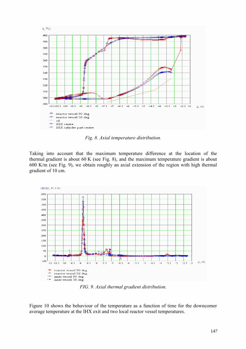
Fig. 8. Axial temperature distribution.

Taking into account that the maximum temperature difference at the location of the thermal gradient is about 60 K (see Fig. 8), and the maximum temperature gradient is about 600 K/m (see Fig. 9), we obtain roughly an axial extension of the region with high thermal gradient of 10 cm.

FIG. 9. Axial thermal gradient distribution.

Figure 10 shows the behaviour of the temperature as a function of time for the downcomer average temperature at the IHX exit and two local reactor vessel temperatures.

147

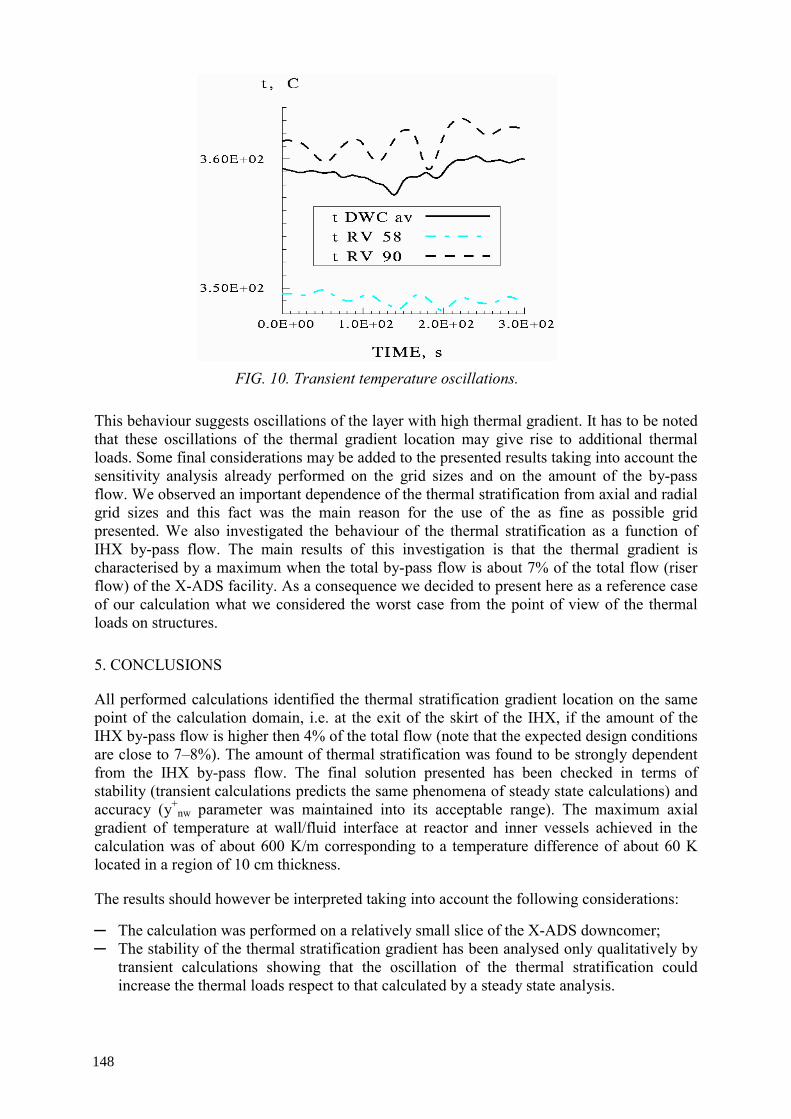
FIG. 10. Transient temperature oscillations.

This behaviour suggests oscillations of the layer with high thermal gradient. It has to be noted that these oscillations of the thermal gradient location may give rise to additional thermal loads. Some final considerations may be added to the presented results taking into account the sensitivity analysis already performed on the grid sizes and on the amount of the by-pass flow. We observed an important dependence of the thermal stratification from axial and radial grid sizes and this fact was the main reason for the use of the as fine as possible grid presented. We also investigated the behaviour of the thermal stratification as a function of IHX by-pass flow. The main results of this investigation is that the thermal gradient is characterised by a maximum when the total by-pass flow is about 7% of the total flow (riser flow) of the X-ADS facility. As a consequence we decided to present here as a reference case of our calculation what we considered the worst case from the point of view of the thermal loads on structures.

5. CONCLUSIONS

All performed calculations identified the thermal stratification gradient location on the same point of the calculation domain, i.e. at the exit of the skirt of the IHX, if the amount of the IHX by-pass flow is higher then 4% of the total flow (note that the expected design conditions are close to 7–8%). The amount of thermal stratification was found to be strongly dependent from the IHX by-pass flow. The final solution presented has been checked in terms of stability (transient calculations predicts the same phenomena of steady state calculations) and accuracy (y+

nw parameter was maintained into its acceptable range). The maximum axial gradient of temperature at wall/fluid interface at reactor and inner vessels achieved in the calculation was of about 600 K/m corresponding to a temperature difference of about 60 K located in a region of 10 cm thickness.

The results should however be interpreted taking into account the following considerations:

─ The calculation was performed on a relatively small slice of the X-ADS downcomer; ─ The stability of the thermal stratification gradient has been analysed only qualitatively by

transient calculations showing that the oscillation of the thermal stratification could increase the thermal loads respect to that calculated by a steady state analysis.

148

Having in mind the above limitations of the present calculations we can say that:

─ The existence of a thermal stratification gradient has been confirmed by the calculations, its location and value determined;

─ The steady state thermal loads as calculated in this analysis have been found acceptable for the reactor and inner vessels;

─ In the case that more refined thermal-hydraulic analysis give rise to unacceptable loads, the introduction of adequate design modifications (for example thermal shields) may be chosen as a final solution.

REFERENCES

[1] RUBBIA, C., et al., Conceptual Design of a Fast Neutron Operated High Power Energy Amplifier, Technical Report CERN/AT/95-44(ET), CERN, Geneva, Switzerland (1995).

[2] ANSALDO, CRS4, ENEA, INFN, Energy Amplifier Demonstration Facility Reference Configuration. Summary Report, Ansaldo Nucleare Report EAB0.001200, Genova, Italy (1999).

[3] CINOTTI, L., Lead-bismuth: critical points for the demo. Tech. R., Ansaldo Nucleare, Genova, Italy (2000).

[4] CORSINI, S., Primary coolant temperature profiles in the downcomer of the ADS-DF, Technical report ADS 5 TRLX 0275, Ansaldo, Genova, Italy (1999).

[5] ARAGONESE, C., et al., A thermal fluid-dynamic steady state analysis of the EADF downcomer channel, Technical Report 00/07, CRS4, Center for Advanced Studies, Research and Development in Sardinia, Cagliari, Italy (2000).

[6] ARAGONESE, C., et al., A thermal fluid-dynamic transient analysis of the EADF downcomer channel, Technical Report 00/84, CRS4, Center for Advanced Studies, Research and Development in Sardinia, Cagliari, Italy (2000).

[7] KIRILLOV, P.L., BOGOSLOVSKAIA, G.P., Heat and Mass Transfer in Nuclear Power Installations. Energoatomizdat, Moscow, Russian Federation (2000) (in Russian).

[8] KIRILLOV, P.L., YURIEV, YU.S., BOBKOV, V.P., Handbook of Thermohydraulic Calculations. Energoatomizdat, Moscow, Russian Federatin (1990) (in Russian).

[9] SUBBOTIN, V.I., IBRAGIMOV, M.X., USHAKOV, P.A., BOBKOV, V.P., YRIEV, Y.S., Hydrodynamics and Heat Transfer in Nuclear Power Installations (basic of calculations), Atomizdat, Moscow, Russia (1975) (in Russian).

[10] KUTATELADZE, S.S., BORISHANSKII, V.M., A Concise Encyclopedia of Heat Transfer, Pergamon Press (1966).

149

EXPERIENCES FROM USING THE STAR-CD CODE FOR Pb/Bi-COOLANT FLOWS

J. CARLSSON, H. WIDER European Commission (EC), Joint Research Centre (JRC), Petten, Netherlands

Abstract

The influence from using different turbulence models for two types of calculations has been investigated. The standard k-ε, the RNG k-ε, the Chen k-ε, the Cubic k-ε, and the Quadratic k-ε turbulence models were examined for a pin bundle and a reactor vessel air-cooling system. It was investigated how the turbulence models affect the heat removal rate from the reactor vessel during a Total-Loss-Of-Power accident in an 80 MW(thermal) Pb/Bi-cooled Accelerator-Driven System. The temperature and velocity profiles in the boundary layer next to the reactor vessel wall were in all three cases modeled with a standard law for the wall function. It was concluded from these STAR-CD calculations that the choice of turbulence model affects the heat transfer rate very weakly for this type of problem. Thereafter, one calculation was run in which the turbulence equations were not solved and yet another one in which the Two-Layer model in the boundary layer was used together with a RNG k-ε turbulence model. These two latter showed reasonably similar results, however, they had about a 20 K lower maximum temperature at core outlet during the transient evolution than the calculations using the law of the wall function. This discrepancy was attributed to the different heat transfer modes used from the liquid to the wall. Earlier two computational fluid dynamics codes, STAR-CD and FLUENT, has been compared for the air-cooling of the reactor vessel. The results for a Total-Loss of Power accident for the 80 MW(thermal) ANSALDO design showed that the temperature peak from these codes differed about 10 K. Furthermore, in the European project called Preliminary Design Study of and Accelerator-Driven System the STAR-CD outcome appears to be in good agreement with other codes like RELAP5/PARCS, SIMMER-ADS, TRAC-M etc. In the pin bundle calculation a discrepancy of about 20% was found with regard to maximum turbulence dissipation and turbulence kinetic energy at core outlet of the Pb/Bi-coolant when different turbulence models were used. The maximum temperature difference at core outlet varies only by 0.8 K for the examined turbulence models. The computational fluid dynamics code STAR-CD was used for all calculations presented in this paper.

1. INTRODUCTION

In 1997 Rubbia et al. used the Computational Fluid Dynamics (CFD) code STAR-CD [1] for thermal hydraulics calculations on the Energy Amplifier (EA) [2]. The code was used to calculate the emergency decay heat removal by air circulation around the guard vessel [3]. Currently CFD codes are used for designing many of the components of heavy metal-cooled reactors or ADSs, e.g., the beam target, to estimate the natural circulation in the primary circuit, and also pin bundle calculations. All the mentioned areas are presently investigated within the European integrated project called Preliminary Design Study of and Accelerator-Driven Systems (PDS-XADS). The PDS-XADS examines both a Pb/Bi-cooled and a He-cooled reactor, both of 80 MW(thermal) power. There are 27 transients examined for the thermal hydraulics calculations, e.g., protected and unprotected Loss-Of-Flow (LOF) and Loss-Of-Heat-Sink (LOHS) accidents. Even though the results are not finalized it is clear that STAR-CD predicts temperatures comparable other codes like RELAP5/PARCS, SIMMER-ADS, TRAC-M. In Sect 0 the theory of the turbulence models employed in this paper is presented. Section 0 contains the geometrical set-up and the modeling tools. The results from calculations on the primary circuit are presented in Sect 0 and the results from the pin bundle calculations in Sect 0. Finally the conclusions are contained in Sect 0.

2. TURBULENCE MODELS

Codes that employ the turbulent Prandtl number to describe the turbulent heat transport (thereby assuming the Reynolds analogy) will compute erroneous results for liquid metals. Each turbulence model has a distinct description of the turbulent heat transport, which

151

contains many parameters whose values depend both on the type of fluid and the flow conditions. Standard values for these parameters are available for common fluids like gases and water but not for liquid metals. Preliminary benchmarks on experiments using liquid metals show that the turbulent parameters contained in CFD codes could be unsuitable for liquid metals [4]. Therefore, measurements of the turbulent quantities in liquid metal flows are needed in order to adjust the turbulence parameters.

Calculations were performed with five turbulence models, i.e., the standard k-ε, RNG k-ε, Chen k-ε, the Cubic k-ε, and the Quadratic k-ε models. The turbulence kinetic energy, k, is estimated with the same equation for all models, see Eqs 1-6 [1].

( ) ( )i

i

i

itBt

jk

effj

j xu

kxu

PPxkku

xkg

tg ∂∂

⎟⎟⎠

⎞⎜⎜⎝

⎛+

∂∂

−−+=⎟⎟⎠

⎞⎜⎜⎝

⎛

∂∂

−∂∂

+∂∂ ρμρεμ

σμ

ρρ32~1

(1)

where

teff μμμ += (2)

ερ

μ μμ

2kCft =

(3)

j

iij x

usP

∂∂

≡ 2 (4)

ith

iB x

gP

∂∂

−≡ρ

ρσ1

, (5)

( )j

iijjiNL x

usuuP

∂∂

−−= 2 (6)

2.1. Turbulence dissipation for standard k-ε model

The turbulence dissipation is modeled for the standard k-ε model as is described in Eq. (7). Cμ,,σk, σε, Cε1, Cε2, Cε3, and Cε4 are constants [1].

( )

( ) NLi

i

i

i

i

itB

j

effj

j

Pk

Cxu

Ck

Cxu

kxu

PCPCk

xu

xg

tg

ερεερρμε

εσμ

ερρε

εεεεε

ε

14

2

231 32

~1

+∂∂

+−⎥⎦

⎤⎢⎣

⎡

∂∂

⎟⎟⎠

⎞⎜⎜⎝

⎛+

∂∂

−+=

=⎟⎟⎠

⎞⎜⎜⎝

⎛

∂∂

−∂∂

+∂∂

(7)

152

2.2. Turbulence dissipation with RNG k-ε model

For the RNG k-ε model the turbulence dissipation is determined with Eqs 8-10. Cμ,,σk,,σε,,Cε1, Cε2, Cε3, Cε4, η0, and β are constants [1].

( )

( )

( )k

C

xu

Ck

Cxu

kxu

PCPCk

xu

xg

tg

i

i

i

i

i

itB

j

effj

j

2

3

03

4

2

231

1

1

32

~1

ρεβη

ηηη

ρεε

ρρμε

εσ

μερρε

μ

εεεε

ε

+

−−

−∂∂

+−⎥⎥⎦

⎤

⎢⎢⎣

⎡

∂∂

⎟⎟⎠

⎞⎜⎜⎝

⎛+

∂∂

−+=

=⎟⎟⎠

⎞⎜⎜⎝

⎛

∂∂

−∂∂

+∂∂

(8)

where

εη kS≡

(9)

( ) 212 ijij ssS ≡ (10)

The last term in the dissipation equation differs from the standard k-ε relative the RNG k-ε model. It represents the effect of mean flow distortion on ε and is supposed to have a more general representation of the turbulence dissipation.

2.3. Turbulence dissipation with Chen’s k-ε model

In Chen’s k-ε turbulence dissipation equation the last term is also different, see Eq. (11) [1].

( )

( )k

PCxu

Ck

Cxu

kxu

PCPCk

xu

xg

tg

ti

i

i

i

i

itB

j

effj

j

2

54

2

231 32

~1

μρεερρμε

εσμ

ερρε

εεεεε

ε

+∂∂

+−⎥⎥⎦

⎤

⎢⎢⎣

⎡

∂∂

⎟⎟⎠

⎞⎜⎜⎝

⎛+

∂∂

−+=

=⎟⎟⎠

⎞⎜⎜⎝

⎛

∂∂

−∂∂

+∂∂

(11)

In the Chen model the production time scale, k/P, and the dissipation time scale, k/ε, are used to close the ε equation. This extra time scale is claimed to allow the energy transfer mechanism of turbulence to respond to the mean strain rate more efficiently.

2.4. Relations for linear models

In the linear models mentioned above the Reynolds stresses are linked to the averaged flow properties analogously to their laminar flow counterparts [1].

ijk

ktijtji k

xu

suu ∂⎟⎟⎠

⎞⎜⎜⎝

⎛+

∂∂

−=− ρμμρ322// (12)

153

jth

tj x

hhu∂∂

−=−,

//

σμ

ρ (13)

j

c

tm

tmj x

mmu

∂∂

−=,

//

σμ

ρ (14)

where

2

//ii uu

k ≡ (15)

the turbulence viscosity is linked to k and ε via

ερ

μ μμ

2kCft = (16)

2.5. Relations for the non-linear equations

Non-linear models can account for anisotropy by adopting non-linear relationships between Reynolds stresses and the rate of strain [1].

For the quadratic model the Reynolds stresses are computed as shown in Eqs (17–25).

[ ] ⎥⎦⎤

⎢⎣⎡ ΩΩ−ΩΩ+Ω+Ω

+⎥⎦⎤

⎢⎣⎡ −+−⎟⎟

⎠

⎞⎜⎜⎝

⎛+

∂∂

=

klklijjkikt

kijkkjikt

klklijkjikt

ijt

ijk

ktji

CSSC

SSSSCSkx

ukk

uu

δεμ

εμ

δεμμδρμρ

31

31

32

32

1

//

(17)

( ) ( ) μμ CScccC

CScccC

NLNL

NL

NLNL

NL3

76

223

76

11 ;

+=

+= (18,19)

( ) μCScccC

NLNL

NL3

76

33 += (20)

and

Ω++=

321

0

ASAAACμ

(21)

where

A0, A1, A2, A3, cNL1, cNL2, cNL3, cNL6, cNL7 are empirical coefficients.

The turbulent viscosity μt is defined in Eq. (16).

i

j

j

iij x

uxuS

∂

∂+

∂∂

= (22)

154

i

j

j

iij x

uxu

∂

∂−

∂∂

=Ω (23)

ijijSSkS21

ε= (24)

ijijk

ΩΩ=Ω21

ε (25)

For the cubic model the Reynolds stresses are computed according to Eq. (16).

[ ]

( ) ( ) ijklklklkltkllikjljkit

klklijjkikt

kijkkjikt

klklijkjikt

ijt

ijk

ktji

SSSkCSSSkC

CSSC

SSSSCSkx

ukk

uu

ΩΩ−+Ω+Ω

+⎥⎦⎤

⎢⎣⎡ ΩΩ−ΩΩ+Ω+Ω

+⎥⎦⎤

⎢⎣⎡ −+−⎟⎟

⎠

⎞⎜⎜⎝

⎛+

∂∂

=

2524

32

1

//

31

31

32

εμ

εμ

δεμ

εμ

δεμμδρμρ

(26)

where

255

244 ; μμ CcCCcC NLNL == (27,28)

where cNL4, and cNL5 are empirical coefficients. S and Ω are calculated according to Eqs (24–25). The turbulent viscosity μt is defined in Eq. (16).

3. GEOMETRICAL SET-UP AND MODELING TOOLS

The CFD code STAR-CD is used for all calculations presented. A second order MARS scheme [1] is used for spatial, turbulence, temperature and density discretization. Time stepping is performed with an implicit scheme.

For the calculations on the Reactor Vessel Air Cooling System (RVACS) the boundary layers were modeled with a standard law of the wall function [1] and three different turbulence models. One RVACS calculation incorporated the Two-Layer model [1] that analytically compute the velocity and temperature profiles. Finally one calculation was performed without solving the turbulence equations. For the pin bundle the Two-Layer model together with the RNG k-ε turbulence models were used for all calculations.

3.1. The Pb/Bi-cooled Accelerator-Driven System of ANSALDO

The Pb/Bi-cooled PDS-XADS design of ANSALDO was used for these investigations. It has a pool-type vessel with a height of 9 m and a 6 m diameter. This design has a low pressure drop core of 80 MW(thermal) power, which is fed by a 3 MW accelerator. The reactor vessel is contained in a guard vessel [5]. In the case of failure of all active heat removal systems the ultimate heat sink for this reactor design is an RVACS. This particular

155

RVACS design is physically separated from the guard vessel in order to minimize the risk for release of radioactive particles to the atmosphere [5]. The heat transfer is by thermal radiation and natural air convection. The computational mesh has about 1200 cells and can be seen in Fig. 1.

FIG. 1. The computational mesh for the Pb/Bi-cooled PDS-XADS of ANSALDO.

3.2. Pin bundle of the Pb/Bi-cooled accelerator driven system of ANSALDO

Also for the pin bundle calculations the PDS-XADS design of ANSALDO is used. The average linear power is 85.2 W/cm. The pin diameter is 8.5 mm and the pitch-to-diameter (PTD) is 13.4 mm. The flow rate at normal operation is ~0.42 m/s through a core channel [5].

Figure 2 illustrates a pin bundle of the PDS-XADS design seen from above. About 15 000 cells are used in the following calculations.

156

FIG. 2. Calculational mesh of a pin bundle from the PDS-XADS design of ANSALDO.

4. RESULTS FROM CALCULATIONS ON THE PRIMARY CIRCUIT

The turbulence models’ affect on the heat removal from the reactor vessel wall has been investigated. The turbulence models examined were the standard k-ε, RNG k-ε, and Chen k-ε models and then the maximum temperatures at core outlet were compared to the heat removal rate. Both a standard wall function and a Two-Layer model were used to estimate the temperature and velocity profiles in the boundary layers. For one case the turbulence equations were not solved, then the energy equations in the solid and the fluid were solved simultaneously at the same time as continuity of the heat flux is enforced.

Figure 3 shows an example of the turbulent kinetic energy using the standard k-ε in the primary circuit. It can be seen that the turbulence kinetic energy maximums are located in the core and in the riser, the latter due to that a swirl has developed there.

Figure 4 illustrates the velocities and normal operation in the primary circuit.

157

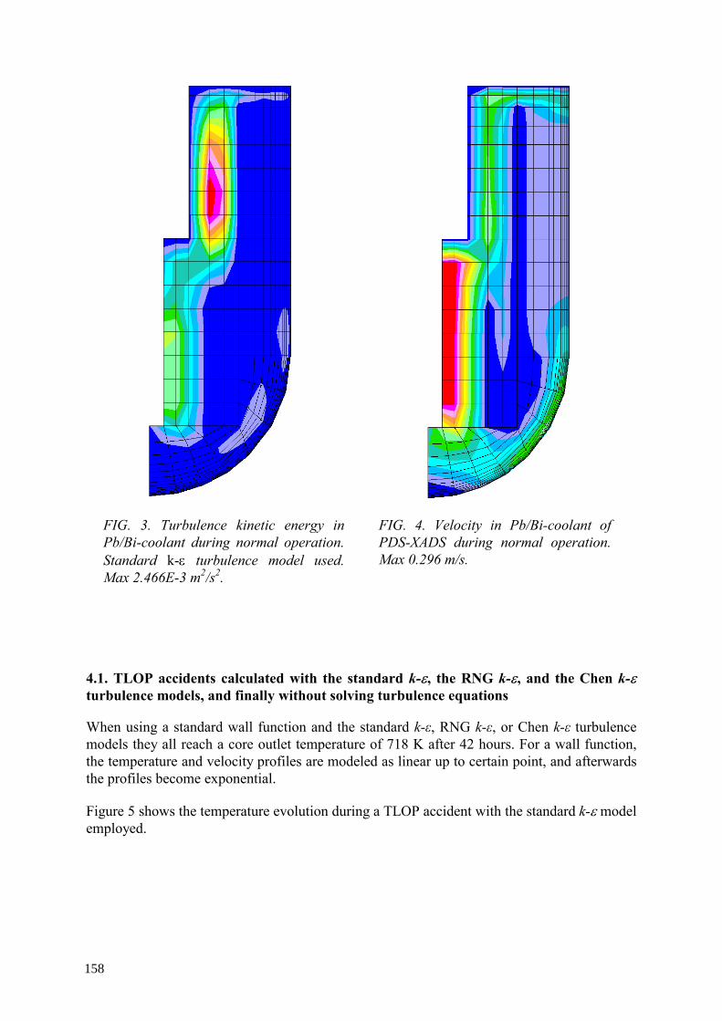
FIG. 3. Turbulence kinetic energy in Pb/Bi-coolant during normal operation. Standard k-ε turbulence model used. Max 2.466E-3 m2/s2.

FIG. 4. Velocity in Pb/Bi-coolant of PDS-XADS during normal operation. Max 0.296 m/s.

4.1. TLOP accidents calculated with the standard k-ε, the RNG k-ε, and the Chen k-ε turbulence models, and finally without solving turbulence equations

When using a standard wall function and the standard k-ε, RNG k-ε, or Chen k-ε turbulence models they all reach a core outlet temperature of 718 K after 42 hours. For a wall function, the temperature and velocity profiles are modeled as linear up to certain point, and afterwards the profiles become exponential.

Figure 5 shows the temperature evolution during a TLOP accident with the standard k-ε model employed.

158

FIG. 5. Temperature and velocity evolution during a TLOP accident without solving the turbulence equations in the Pb/Bi-coolant.

For reasons of comparison a TLOP accident was calculated without solving the turbulence equations too. Then the core outlet temperature peaks at 696 K after about 42 hours (see Fig. 6).

FIG. 6. Temperature and velocity evolution for a TLOP accident. Turbulence equations are switched off.

The Two-Layer model calculates the temperature and velocity profiles in the boundary layers next to walls analytically. A requisite to achieve with acceptable accuracy are refined meshes in the boundary layers, i.e. about 15 cell layers normal to the wall [1].

159

The RNG k-ε turbulence model was used for the turbulence. Figure 7 illustrates the temperature evolution for a TLOP accident. It is to be noted that the temperature evolution matches very well for the case where the turbulence equations were not solved. This is probably only true for cases where the temperature difference between the wall surface and the bulk of the flow are small, in this case they were only about 6 K.

FIG. 7. Temperature and velocity evolution during a TLOP accident using a two layer heat transfer model and the RNG turbulence model.

The results from the calculations are compiled in Table 1.

TABLE 1. MAXIMAL TURBULENCE ENERGY AND DISSIPATION IN THE Pb/Bi-COOLANT DURING NORMAL OPERATION

Heat transfer model

Turbulence model

Max. turbulence

energy, m2/s2

Max. turb. dissipation,

m2/s3

Max. temperature,

K

Standard wall function

Standard k-ε 2.466E-3 2.880E-4 718

Standard wall function

RNG k-ε 1.442E-3 1.362E-4 718

Standard wall function

Chen k-ε 1.375E-3 1.689E-4 718

Two-layer model RNG k-ε 1.445E-3 1.360E-4 696

Static enthalpy - - - 696

160

5. RESULTS FROM THE PIN BUNDLE CALCULATIONS

For all pin bundle calculations the Two-Layer model was used to calculate the heat transfer from the cladding wall to the coolant. Five turbulence models were tried on the same geometry, i.e. the standard k-ε turbulence model, RNG k-ε, Chen k-ε, Cubic k-ε, and finally the Quadratic k-ε turbulence model. Figure 8 illustrates a typical temperature field at core outlet. The standard k-ε turbulence model was used. Next to the cladding surface the maximal temperature is 760.7 K whereas in the bulk of the flow the temperature is about 730 K.

FIG. 8. The temperature field in a coolant at core outlet using the standard k-ε turbulence model.

Figures 9 and 10 show the turbulence kinetic energy and the turbulence dissipation at core outlet while using the standard k-ε turbulence model.

FIG. 9. The turbulence kinetic energy at core outlet using the standard k-ε turbulence.

161

FIG. 10. The turbulence dissipation calculated with the standard k-ε turbulence model.

The results, with regard to the maximum turbulence kinetic energy, turbulence dissipation, and temperature at core outlet, for the standard k-ε, RNG k-ε, Chen k-ε, Cubic k-ε, and the Quadratic k-ε models are compiled in Table 2. The maximum turbulence kinetic energy and turbulence dissipation varies ~20% for the models investigated. The maximum temperature in the Pb/Bi coolant varies with about 0.8 K.

TABLE 2. THE TURBULENCE KINETIC ENERGY AND DISSIPATION CALCULATED WITH THE STANDARD k-ε, RNG k-ε, CHEN k-ε, CUBIC k-ε, AND THE QUADRATIC k-ε MODELS

Max. turbulence kinetic energy,

m2/s2

Max. turbulence dissipation,

m2/s3

Max. temperature, K

Standard k-ε 2.090E-3 0.5505 760.7

RNG k-ε 1.976E-3 0.4319 761.2

Chen k-ε 2.016E-3 0.5171 760.4

Cubic k-ε 2.042E-3 0.4149 761.0

Quadratic k-ε 2.041E-3 0.4142 761.0

162

6. CONCLUSIONS

The standard k-ε, RNG k-ε, and Chen k-ε turbulence models have been used for calculating reactor vessel air cooling by natural convection during a Total-Loss-Of-Power accident. It was shown that all turbulence models give very similar results for this case, i.e. all turbulence models show a temperature peak at core outlet of 718 K. For all these cases the standard law of the wall function was used to model the temperature and velocity profiles in the boundary layers.

If the turbulence equations are not solved the temperature will instead peak at 696 K. And if the Two-Layer model, which solves the temperature and velocity profiles analytically, together with the RNG k-ε turbulence equations the core outlet temperature peaks at 696 K too. The difference in temperature compared to the cases where the law of the wall function is employed is not due to the turbulence models, but due to the heat transfer modes.

The standard k-ε, RNG k-ε, and Chen k-ε, the Cubic k-ε, and the Quadratic k-ε turbulence models were used for the pin bundle calculations. The maximum turbulence energy and the turbulence dissipation vary by ~20%, and the coolant maximum temperature at core outlet varies with ~0.8 K.

REFERENCES

[1] Computational Dynamics Ltd., Methodology Volume 3.10 (1999) and http://www.cd-adapco.com/products/starsolver.htm

[2] RUBBIA, C., et al., Conceptual design of a fast neutron operated high power every amplifier, CERN/AT/95-44, Geneva, Switzerland (1995).

[3] BUONO, S., RUBBIA, C., Simulation of a Total Loss of Power accident in the Energy Amplifier, CERN/ET Internal note 96-015, Geneva, Switzerland (1996).

[4] ARIEN, B., ASCHLIM: A 5th FP Project for the assessment of CFD codes applied to heavy liquid metals, Proc. Int. Workshop on P&T and ADS Development 6-8 October 2003, SCK•CEN, BLG-959, ISBN 9076971072, Mol, Belgium (2003).

[5] ANSALDO NUCLEARE, XADS Pb-Bi Cooled Experimental Accelerator Driven System – Reference configuration, Summary report, ADS 1 SIFX 0500 – Rev 0 (June 2001).

163

CFD SIMULATION OF SINQ HETSS MERCURY EXPERIMENTS

T.V. DURY Paul Scherrer Institut (PSI), Villigen, Switzerland

Abstract

The SINQ HETSS target experiments were designed to study the heat transfer process between flowing mercury and a heated surface, in the spallation target geometry suitable for installation in the PSI SINQ neutron source. The basic test-section consisted of a vertical cylinder containing an outer annulus for downward inlet fluid flow, with a hemispherical dome at the bottom (the window), through which a proton beam would pass vertically upwards into the target when installed in SINQ. Return fluid flow was upwards through the central region of the cylinder. In this experimental series, the target window was equipped with a strip of HETSS (Heat Emitting Temperature Sensing Surface) devices, to enable local heat transfer coefficients to be measured on the inner window surface. Using a different window construction, velocity profiles of mercury within the dome region were obtained by the use of the Ultrasonic Doppler method (UVP), which provides time-averaged local velocities as well as local flow fluctuation information. The goal of this present study was to examine the ability of the commercial CFD code CFX-4.4 to predict the velocity fields within the lower region of the target, and assess the performance of standard turbulence models in simulating the heat transfer between the internal fluid and the target window when used for this typical heavy liquid metal. The layout of internal geometry was one with a slanted end at the bottom of the guide tube, which separates the annulus and riser regions of the target. Mercury flows simulated were 1.2 and 3.6 L/s. Comparison is made between experimental and CFD-derived window heat transfer and velocity patterns. Different turbulence models and turbulent Prandtl Number were employed in CFX-4.4, with meshes with a different degree of refinement, in particular at the window. Results give an indication of the best turbulence models and degrees of mesh refinement to use in this particular situation. This is of current relevance to the MEGAPIE target, which is currently being designed and constructed for insertion in SINQ, using lead-bismuth eutectic as the coolant fluid, and for the general application of this target design n Accelerator Driven Systems (ADS), an innovative design of nuclear reactor which can be used for the production of energy as well as the burning and reduction of toxic reactor waste.

1. INTRODUCTION

The SINQ HETSS (Heat Emitting Temperature Sensing Surface) target experiment was performed at the Institute of Physics, University of Latvia, Riga. It was designed to measure velocity fields and heat transfer in the window region of a spallation target geometry suitable for installation at the PSI SINQ neutron source.

The basic test-section consisted of a vertical cylinder containing an outer annulus for downward inlet fluid flow, with a hemispherical dome at the bottom (the window), through which a proton beam would pass vertically upwards into the target when installed in SINQ. Return fluid flow was upwards through the central region of the cylinder – the riser. The tests studied here had an internal design in which the end of the shell separating the annulus fluid and that in the riser (called the guide tube) was slanted at its bottom edge.

Although the target fluid in SINQ would have to be another material than mercury, because of its poor neutronic absorption characteristics for a source providing a constant supply of neutrons, such as SINQ or a target functioning as an integral part of an Accelerator Driven

System reactor (ADS), mercury has the great benefit that it is liquid at room temperature, thereby greatly simplifying experimentation. It also has physical properties that are similar enough to enable it to be a suitable alternative for heat transfer study and fluid velocity measurements.

The goal of this study was to examine the ability of the CFD code CFX-4.4 to predict the velocity fields measured within the lower region of the target, and assess the performance of

165

standard turbulence models in simulating the heat transfer between the target window and the internal fluid when used for a typical heavy liquid metal.

A sketch of the test-section, including upper manifolds, is shown in Fig. 1. A detailed cross-section of the lower target region is given in Fig. 2, but without the flanges connecting the window dome to the cylindrical body of the test-section.

5

00

Outlet chamberHg Out

Inlet chamberHg InHg In

300

1

623

Bypass Tube

2.87

94

.0 1

029.

0

2.0

5.0

5

5.025

.0

207.0

207.0

mm

6.0

50

0.0

R103.5

126.0

126.0

FIG. 1. Complete test-section. FIG. 2. Cross-section through

lower test-section with 20-mm guide-tube/window gap.

It was considered unnecessary to model these as all calculations were for steady-state conditions, and the tests were essentially isothermal, with only a small amount heat added through the HETSS devices (bulk fluid temperature, with a mercury flow of 1.2 L/s, only rose by 0.26°C, on average, as a result of the heat added by the HETSS). The inlet manifold is shown in close-up in Figs 3 and 4.

Incoming flow enters through the radial pipes, into a ring annulus that is closed at the bottom. The fluid expands upwards, passes over the inner wall of the annulus, is redistributed as it passes by blockage cylinders hanging vertically inside the inner annulus, and passes vertically downwards into the annular inlet to the lower test-section. The lower end of each hanging cylinder is sealed, preventing fluid entering the cylinders.

166

InletInletO

utlet

ø300ø490

500

ca. 150 ca. 150ø410

50

5

77

ø8960°

150

ø89

245

205

5.0

32.0

Cylinders sealed at bottom

Y

Z

FIG. 3. Side view cross-section of manifold,with outer walls.

FIG. 4. Plan view cross-section of manifold, with outer walls.

2. EXPERIMENTAL SETUP AND CONDITIONS

The test-section window was equipped with a strip of HETSS [1, 2] devices (Fig. 5), to enable local heat transfer coefficients to be calculated on the inner window surface.

Pump

Target

Orientation 120 deg.

Electricalconections

91112

1314

1516

1718

1920

21

Sealing(insures turnability)

TurnableHETSSinsert

1357

Orientation of theturnableHETSS insert 0 deg.

Orientation 60 deg.

Orientation 90 deg.

g

vertical gap between the central tube end and hemisphericasurface

FIG. 5. 3-D view of HETSS installation.

167

Using a different window construction, velocity profiles of mercury within the dome region were obtained by the use of the Ultrasonic Doppler method (UVP), which provides time-averaged local velocities as well as local flow fluctuation information [3].

The inlet temperature and heat flux conditions on each HETSS device were 10°C and 70 000 W/m2, respectively. Total flows of 1.2 and 3.6 L/s were imposed during tests. The vertical separation distance between the end of the guide tube and the window was in the range 40 mm ± 15 mm.

The corresponding physical properties were taken either directly from values at 10°C listed in [4], or obtained by linear interpolation from tabulated values at 0 and 20°C. The values used for these CFD simulations, performed with constant properties, are given in Table 1.

TABLE 1. PHYSICAL PROPERTIES OF MERCURY AT 10°C

Physical parameter Symbol Magnitude

Density, kg/m3 ρ 13570.4

Dynamic viscosity, kg/ms μ 1.6215×10-3

Thermal conductivity, W/mK λ 8.3125

Specific heat, J/kgK Cp 140.0

Thermal expansion coefficient, 1/K β 1.813×10-4

Prandtl number Pr = Cp⋅μ / λ 0.027

3. CFD MODEL

Examination of velocity profiles measured around the annulus during experiments with a flat end to the guide tube revealed that the profile was not flat as the fluid approached the bottom of the test-section. Thus, for the majority of these CFD simulations, the inlet manifold system was also modelled and fluid mass flow was equally distributed to the six inlet pipes (each of which was modelled as 150 mm in length), with a flat velocity profile applied at each inlet plane. It was considered unnecessary to model the outer test-section walls and its flanges (Figs 6 and 7), as the total heat deposition was very low in the HETSS measurement tests, which were preconditioned and performed under steady-state conditions, and the experiments for velocity measurement were carried out under isothermal conditions, as far as possible. However, the guide-tube wall thickness and the thicknesses of all internal components within the inlet manifold were represented.

The HETSS strip was located along the angle of maximum slant of the end of the guide tube, with the elements numbered from 1 at the end with the smallest gap to 21 at the side with the largest gap. Each HETSS element was 10 mm in length (measured along the strip) and 40 mm in width (across the strip).

168

2.0

5.0

5

5.025

.0

207.0

207.0

10.0

mm

11

23.0

50

0.0

R103.5

126.0

126.0

HETSS 1HETSS 21

HETSS Strip

FIG. 6. Cross-section of lower target, in plane of HETSS strip; no hull thickness.

2.0

5.0

207.0

207.0

40.0 4 0

.0

mm

50

0.0

11

23.0

HETSS

R103.5

126.0

126.0

FIG. 7. HETSS strip aligned in direction of view; no hull thickness.

The requirement of CFX-4.4 of a structured mesh meant that the mesh distribution across each pipe diameter could not be as fine as necessary to obtain a high accuracy of velocity profile, otherwise an unacceptably high number of mesh cells for the whole model would have resulted. Nevertheless, it was considered that a profile with 4 cells across a diameter was adequate, as the effect on the flow of the upstream bends in the experimental facility, together with the redistribution of the flow caused by striking the vertical wall immediately inside the manifold, would make further refinement of less importance than having a fine fluid cell thickness at the surface of this vertical wall (the fluid cell thickness at the wall where the inlet fluid impinged was 1.5 mm, in all models). The model mesh is shown in Figs 8 and 9, in vertical cross-section through the inlet manifold region and in horizontal cross-section through the centre of the inlet pipes, respectively.

Due to the structured mesh required for this model, the relative sizes of meshes shown in Figs 8 and 9 vary by a large factor. This is particularly evident as the effect of radius makes the cells further from the vertical target axis larger than those nearer the axis. Also, the requirement of fine meshes in the lower region of the target results in a very fine mesh close to the target axis.

In order to determine the effect of fluid mesh size next to the HETSS devices and in the annulus, models with different degrees of mesh refinement were generated. These are listed in Table 2, together with the turbulence models applied with the different meshes.

169

FIG. 8. Vertical section on centreline of model: inlet manifold region.

FIG. 9. Horizontal section through centre of inlet pipes.

Target window cell distributions for Models A, B and C are shown in Figs 10 - 12, respectively, to show the relative sizes of the fluid cell thicknesses adjacent to the HETSS. Cutaway perspectives of the whole and lower regions of the test-section for Model C are shown in Figs 13 and 14, respectively.

TABLE 2. MODEL MESHES, y+ RANGE AND TURBULENCE MODELS APPLIED; 1.2 L/s FLOWRATE

Calculation Mesh

designation Total cells y+ range over HETSS strip Turbulence model

1 A 239 256 10 → 100 Standard k-ε ( PrTurb = 0.9 )

2 B 336 120 14 → 52 Standard k-ε ( PrTurb = 0.9 )

3 C 451 800 6 → 28 Standard k-ε ( PrTurb = 0.9 )

4 C 451 800 8 → 26 Standard k-ε ( PrTurb = 2.0 )

5 C 451 800 1 → 10 Menter-modified k-ω

For all of the calculations reported here, the advection terms were determined using a hybrid differencing scheme which is the default in CFX-4.4. This has the advantage of robustness, but is only first-order accurate. However, it is slightly better than an upwind differencing method, because second-order central differencing is used across streams and in regions of low flow, an important aspect of some regions in this facility.

170

FIG. 10. Model A. FIG. 11. Model B. FIG. 12. Model C.

FIG. 13. Sectional view of test-section.

FIG. 14. Sectional close-up of lower target showing HETSS strip (shaded red) and guide tube with slanted end.

171

4. RESULTS

4.1. Flow-rate 1.2 L/s

Calculations 1 to 5 were performed with a flow of 1.2 L/s using the following turbulence models, depending on the level of refinement of the mesh model employed:

─ Standard k-ε model, with standard coefficients [6] (in particular, PrTurb = 0.9); ─ Standard k-ε model, but with PrTurb = 2.0; ─ Menter-modified k-ω model [9, 10].

To examine the influence of the turbulent Prandtl Number for enthalpy (PrTurb) incorporated in the standard k-ε model, it was changed from the standard value of 0.9 to 2.0, for one simulation with Mesh C. For all calculations, the influence of buoyancy was incorporated by using the Boussinesq approximation.

The Menter-modified k-ω model incorporated as an option in CFX-4.4 is a development of the standard k-ω model of Wilcox [11], with the modification introduced to switch from the standard k-ω model close to walls to equations equivalent to the standard k-ε model away from walls, but using the independent variables k and ω. This treatment is more robust than the standard low-Reynolds number k-ε model, and requires a less-fine distribution of fluid cells normal to heating or cooling surfaces.

For simplicity, heat transfer results are compared with experimental data in the form of temperature difference between the HETSS patches on the target window and the bulk fluid (taken to be the same as that of the inlet fluid). In the experiment, temperatures are averaged over the surface area of each individual HETSS device. However, it was not possible to define a separate patch for each individual HETSS element in the CFD model, due to the geometrical complexity at the bottom of the target, and the strip was thus divided into 5 separate axial zones. This allowed temperatures from the CFX-4.4 calculation to be picked up across the HETSS width at each location of model mesh cells along the length of the HETSS patch strip, and a width-average for each cell position along its length to be calculated. This resulted in a more continuously varying distribution of temperature along the length than indicated by the HETSS measurements themselves, where each HETSS element temperature was an averaged over the area covered by the 4 cm width and 1 cm length of each unit. Otherwise, results are comparable, and the CFD values show the temperature profile along the strip in finer detail than with the subdivision of the HETSS.

4.1.1. Standard k-ε turbulence model, PrTurb = 0.9 or 2.0

Examining the results of CFD simulations using the standard k-ε model, with turbulent Prandtl Number of 0.9 and 2.0, temperature distributions at the bottom of the target, in a vertical section through the length of the HETSS strip (through its centre), are shown as shaded contours for calculations 1 to 4, in Figs 15 to 18, respectively.

172

FIG. 15. Temperatures on HETSS centreline plane: 1.2 L/s, k-ε model,

Calc. 1, PrTur = 0.9.

FIG. 16. Temperatures on HETSS centreline plane: 1.2 L/s, k-ε model,

Calc. 2, PrTurb = 0.9.

FIG. 17. Temperatures on HETSS centreline plane: 1.2 L/s, k-ε model,

Calc. 3, PrTur = 0.9.

FIG. 18. Temperatures on HETSS centreline plane: 1.2 L/s, k-ε model,

Calc. 4, PrTurb = 2.0.

With PrTurb = 0.9 (Figs 15 to 17), two effects of mesh refinement on the temperature distribution are visible in these cross-sectional plots. The first is that the hot fluid layer next to the wall along the length of the HETSS strip, with the coarse mesh (A), is of almost constant thickness (effective thermal diffusion), but with the finest mesh (C) the thickness of the hot fluid layer varies considerably along the strip. Secondly, tongues of fluid that are visibly hotter than the bulk emanate from the regions on the strip inside the guide-tube radius. The penetration of these tongues into the riser region increases as the mesh is refined. With the finest mesh, the penetration is approximately twice as far as with the coarse mesh. Thus, refining the mesh appears to significantly prevent numerical diffusion of enthalpy, and should allow more accurate simulation of reality.

The influence of increasing the value of PrTurb to 2.0, with the finest mesh, is to reduce the extent of penetration of the tongues of hotter fluid into the riser, while also causing the maximum wall temperature to rise (i.e. decrease the heat transfer coefficient into the fluid). Otherwise, the general thermal pattern is similar to that shown for the case when PrTurb = 0.9.

The temperature distributions over the HETSS surface, viewed from below, with the wide gap on the right-hand side of the plot, are shown for the cases with PrTurb of 0.9 in Figs 19 to 21, for the coarse, intermediate and fine mesh cases, respectively. To aid interpretation, the

173

outline of the guide tube is superimposed on the temperature plot, and is visible as two concentric rings. The largest gap between guide tube and window is on the right-hand side of each of these figures. The calculation with PrTurb of 2.0 is shown in Fig. 22.

FIG. 19. Temperatures on HETSS surface: 1.2 L/s, k-ε model, Calc. 1, PrTurb = 0.9.

FIG. 20. Temperatures on HETSS surface: 1.2 L/s, k-ε model, Calc. 2, PrTurb = 0.9.

FIG. 21. Temperatures on HETSS surface:

1.2 L/s, k-ε model, Calc. 3, PrTurb = 0.9. FIG. 22. Temperatures on HETSS surface:

1.2 L/s, k-ε model, Calc. 4, PrTurb = 2.0.

The cylindrical and spherical geometry of the annulus and window cause a horse-shoe temperature distribution on the HETSS under the largest gap, with Mesh C. This shape is slightly asymmetrical, as is the distribution over the rest of the strip, showing that the flow in the dome is not perfectly symmetrical. In practice, this would be expected to be a region of unstable equilibrium in the flow, and the numerical simulation also appears to exhibit similar behaviour. There is also an asymmetric tongue of hotter fluid leaving the side of the HETSS strip under the edge of the guide tube near the small gap. This indicates clockwise swirl in the fluid in this region (viewed from below), which is just hinted at below the edge of

174

the guide tube at the opposite side of the strip. The presence of asymmetry in the fluid flow distribution will be looked at later in this section.

With the other meshes, the behaviour of the fluid is not entirely consistent as mesh refinement decreases. The intermediate mesh shows a reduced tongue of higher temperature above the HETSS but a strongly enhanced one below it, while both tongues almost disappear with the coarse mesh. On the strip itself, the contours of highest temperature (under the large gap) are modified in both cases, with asymmetry across the strip tending to increase as the mesh becomes coarser. The effect of raising the value of PrTurb is primarily seen as larger temperature gradients on the HETSS strip.

Temperatures along the strip, for the three meshes and with PrTurb of 0.9, are plotted in Fig. 23, together with the experimental data. Both are evaluated as average values over the width of each HETSS device. The experimental data measured over each separate device are plotted as single points at the centre of each, while the CFD results are area-weighted averages over the cells across the HETSS units at every mesh-model cell position along the strip. With the CFD models, there is finer subdivision of the strip than with the HETSS themselves, even with the coarse-mesh model, but results ought not to be significantly different between experiment and simulation.

0

5

10

15

20

25

30

35

0 1 2 3 4 5 6 7 8 9 10 11 12 13 14 15 16 17 18 19 20 21

Distance along HETSS strip [cm]

Tem

pera

ture

diff

eren

ce [º

C]

Finest meshIntermediate meshCoarse meshExperimentHETSS 1

FIG. 23. Temperatures along HETSS strip, 1.2 L/s, Standard k-ε turbulence model.

The experimental data plotted in Fig. 23 show that there is better heat transfer near the centre of the dome than under the edge of the guide tube, where the fluid velocity is higher, at the end of the strip with the low-number HETSS. However, there is not significant evidence from the measured data that such a reduction of heat transfer occurs near the other end of the strip.

With the fine-mesh model, CFD simulation gives a wall temperature that is about 20% higher at the first HETSS unit (i.e. 20% poorer heat transfer) than indicated experimentally. Agreement is quite close in the region from the narrow gap to around two-thirds of the strip

175

length, but major disagreement appears where the fluid passes under the largest gap, where predicted HETSS temperatures are about 50% higher than those measured. This tendency occurs with all degrees of mesh refinement, though the shape of the profile is not consistent with the different meshes.

With the intermediate mesh the peak is sharper, while with the coarse mesh it is flatter. The effect of mesh distribution on surface heat transfer is very obvious, with the temperature difference between the HETSS and the bulk fluid calculated using the coarse mesh being on average about twice as large as that when the fine mesh was used. All the CFD-generated curves show roughly the same trend of shape of distribution, but the fine-mesh case is closest to the experimental data.

4.1.2. Standard k-ε and Menter-modified k-ω turbulence models vs. experiment

Studies reported in [10] suggest that, with a mesh as fine as that used here, the fluid cell size next to the heated strip should be in the correct range to allow this k-ω model to function as intended. Results are compared in Fig. 24 for this model, the standard k-ε model and the experimental data. Agreement of the measured data and the k-ω model is almost perfect at the first HETSS unit along the heated strip, but further along it the k-ω temperatures are always below the measured values and generally below those from the k-ε model. The peak under the narrowest gap is almost captured, but the heat transfer is too high over the remainder of the strip. The flatter profile of the k-ω results agrees better with the measured data over the range HETSS 8 to 21, although the temperatures are too low, and the large temperature peak of the k-ε model under the large gap is almost absent. Nevertheless, it is not obvious why the neat transfer under the guide tube with the k-ω model should differ so significantly between one end of the strip and the other.

0

5

10

15

20

25

0 1 2 3 4 5 6 7 8 9 10 11 12 13 14 15 16 17 18 19 20 21

Distance along HETSS strip [cm]

Tem

pera

ture

diff

eren

ce [º

C]

Menter modified k-omega

Standard k-eps

ExperimentHETSS 1

FIG. 24. Temperatures along HETSS strip, 1.2 L/s (k-ε and Menter-modified k-ω models).

176

Plotting the temperature on a vertical cross-section near the window (Fig. 25), and comparing with the results illustrated in Fig. 17 for the standard k-ε model, it can be seen that there are many differences between the temperature distributions generated by the two models. Firstly, the thickness of the hot fluid layer next to the surface is much greater with the k-ω model over the regions that previously were very thin with the k-ε model (i.e. near the bottom of the dome). This suggests that there has been a modification to the velocity field. Secondly, and confirming a change in the velocity field, there is now much stronger penetration of hot fluid up into the riser on the side of the small gap, driven by fluid entering from the opposite side. Thirdly, the previous tongue of hot fluid rising from below the large gap is now missing completely, showing that there is stronger transverse flow from the large gap, and the flow does not turn as rapidly upwards into the riser. This reinforces the tongue rising from the small-gap side. Comparing the plot of window surface temperature (Fig. 26) with the previous results (Fig. 21), it is clearly seen that the temperature pattern is now symmetrical and the peaks occur on the axial centre-line of the HETSS strip. The symmetry suggests that boundary layer temperatures calculated with the k-ω model are more damped than with the k-ε model. However, velocity patterns with both models will be examined in Section 4.1.4 to check whether there has been any damping of the flow pattern in the annulus to create or assist this stabilisation. The region of high temperature near the narrow gap is now displaced a little towards the centre of the target and is broader and flatter than with the k-ε model.

FIG. 25. Temperatures on HETSS centreline plane: 1.2 L/s, k-ω model, Calc. 5.

FIG. 26. Temperatures on HETSS surface: 1.2 L/s, k-ω model, Calc. 5.

In general, the surprising result from both CFD simulation and experiment is that the heat transfer in the centre of the window dome is better than under the edges of the guide tube, and under the narrow-gap edge in particular. Nevertheless, comparing results between fine-mesh predictions and experiment, the behaviour of neither turbulence model gives what can be assessed as good agreement, over the whole length of the heated strip.

Application of a low-Re turbulence model could show if the currently most accurate two-equation models can accurately simulate the thermal process at the window surface in this target geometry. However, this could not be attempted in the present study because of the limitation of computing resources available to deal with the very high number of model mesh cells necessary when refining the mesh to the level needed for applying the low-Re model, for which it is recommended [7] that there should be between five and ten mesh points between the wall and the dimensionless wall distance 20=+y , giving an order of magnitude more cells than for a mesh with which the standard k-ε model can be used.

177

4.1.3. Boundary layer cell thickness

The thickness of the boundary layer fluid cell has a very strong influence on the heat transfer from the surface to the fluid. This can be seen from observation of the temperatures along the HETSS in Figs 15 to 17. According to the CFD Best Practice Guidelines [7], the logarithmic wall functions used with the standard k-ε turbulence model can only be applied with confidence when the fluid cell adjacent to a surface fulfils the criterion that the dimensionless wall distance +y of the centre of the cell from the wall is in the range:

12030 << +y (1)

This has been defined for both momentum and thermal boundary layers, on the basis that both are similar (Reynolds’ Analogy). However, for a low-Prandtl-Number fluid, such as a liquid metal, this basis is not fulfilled, hence the goal of this study, which was to assess the validity of a current CFD code and its turbulence models when used to simulate such a fluid. CFX-4.4 calculates the value of +y in the model, and the results can be plotted on all fluid/solid interfaces. These values are based on the shear stress and turbulent kinetic energy calculated at the wall, and are thus values to be associated with the momentum boundary layer.

The lower limit for the thermal boundary layer was calculated by CFX-4.4 for these experimental conditions to be 267.5, and for the momentum boundary layer to be 11.22. It can thus be seen that there is a significant difference between these two dimensionless distances, and the condition cannot be satisfied for the thermal boundary layer for the standard k-ε turbulence model if the condition for the momentum boundary layer is also satisfied.

To examine the boundary layer thickness in these models, values of +y were first taken from the recorded CFX-4.4 results at the cross-section indicated A to D in Fig. 27.

FIG. 27. Location of model zones at which +y values are evaluated, HETSS centreline plane, 1.2 L/s flow.

178

The points at which the values were evaluated are all in the same vertical plane, through the centre of the target in the direction of maximum slant angle of the end of the guide tube (i.e. in the plane through the centre of the HETSS strip), and are:

─ At the outer wall of the annulus, at the level where the curved window joins the vertical, cylindrical test-section wall, above the highest point of the slanted edge;

─ In the riser, at the same vertical level and at both sides, to enable comparison to be made between CFX-4.4 values at the two points and the mean value for the whole riser calculated by Eq. (2);

─ At the outer wall, where the area of cross-section for flow at the smallest gap (over the window, on the centreline along the length of the HETSS strip) is a minimum;

─ At the outer wall, at the area of minimum flow cross-section at the largest gap.

The values of +y calculated by the code are listed in Tables 4 to 6 for the three meshes used,

along with the actual cell thickness at these points and the values of +y calculated on the basis of an analytical treatment by Smith [8], which uses the mean flow through a duct section (assuming a thin boundary layer and flow parallel to the wall) and the equation:

μρ BVyyy 42.0)9ln( =++ (2)

where =ρ fluid density, =V free-stream fluid velocity parallel to the wall, =By distance from the wall to the centre of the CFX fluid cell adjacent to the wall, and =μ fluid dynamic viscosity.

It has been assumed in calculating the values using Eq. (2) that =V mean fluid velocity through the cross-sections A to D, with the additional assumption that the vertical flow-rate per unit flow area in the annulus is the same everywhere around the target. This last assumption is an approximation, but due to the relatively large apertures for flow out of the annulus it is accurate enough to enable qualitative comparison to be made between the CFX-4.4 values and those obtained from Eq. (2).

TABLE 4. COMPARISON OF +y VALUES FOR CALCULATION 1, 1.2 L/s FLOW, STANDARD k-ε TURBULENCE MODEL: COARSE MESH MODEL

Position A B C D

Wall cell thickness (mm) 6.59 2.89 3.04 5.87

+y (CFX-4.4) 37 19 (D side)

50 (C side)

29 39

+y (from (Eq.) 2) 97 75 96 99

179

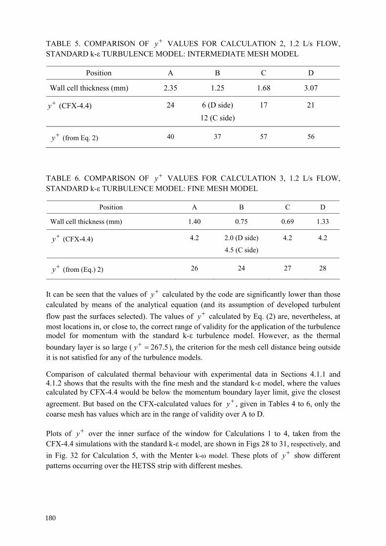
TABLE 5. COMPARISON OF +y VALUES FOR CALCULATION 2, 1.2 L/s FLOW, STANDARD k-ε TURBULENCE MODEL: INTERMEDIATE MESH MODEL

Position A B C D

Wall cell thickness (mm) 2.35 1.25 1.68 3.07

+y (CFX-4.4) 24 6 (D side)

12 (C side)

17 21

+y (from Eq. 2) 40 37 57 56

TABLE 6. COMPARISON OF +y VALUES FOR CALCULATION 3, 1.2 L/s FLOW, STANDARD k-ε TURBULENCE MODEL: FINE MESH MODEL

Position A B C D

Wall cell thickness (mm) 1.40 0.75 0.69 1.33

+y (CFX-4.4) 4.2 2.0 (D side)

4.5 (C side)

4.2 4.2

+y (from (Eq.) 2) 26 24 27 28

It can be seen that the values of +y calculated by the code are significantly lower than those calculated by means of the analytical equation (and its assumption of developed turbulent flow past the surfaces selected). The values of +y calculated by Eq. (2) are, nevertheless, at most locations in, or close to, the correct range of validity for the application of the turbulence model for momentum with the standard k-ε turbulence model. However, as the thermal boundary layer is so large ( 5.267=+y ), the criterion for the mesh cell distance being outside it is not satisfied for any of the turbulence models.

Comparison of calculated thermal behaviour with experimental data in Sections 4.1.1 and 4.1.2 shows that the results with the fine mesh and the standard k-ε model, where the values calculated by CFX-4.4 would be below the momentum boundary layer limit, give the closest agreement. But based on the CFX-calculated values for +y , given in Tables 4 to 6, only the coarse mesh has values which are in the range of validity over A to D.

Plots of +y over the inner surface of the window for Calculations 1 to 4, taken from the CFX-4.4 simulations with the standard k-ε model, are shown in Figs 28 to 31, respectively, and in Fig. 32 for Calculation 5, with the Menter k-ω model. These plots of +y show different patterns occurring over the HETSS strip with different meshes.

180

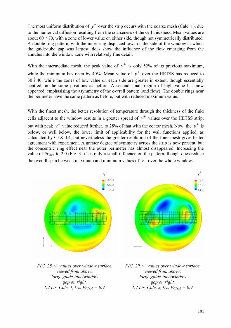
The most uniform distribution of +y over the strip occurs with the coarse mesh (Calc. 1), due to the numerical diffusion resulting from the coarseness of the cell thickness. Mean values are about 60 ⎬ 70, with a zone of lower value on either side, though not symmetrically distributed. A double ring pattern, with the inner ring displaced towards the side of the window at which the guide-tube gap was largest, does show the influence of the flow emerging from the annulus into the window zone with relatively fine detail.

With the intermediate mesh, the peak value of +y is only 52% of its previous maximum,

while the minimum has risen by 40%. Mean value of +y over the HETSS has reduced to 30 ⎬ 40, while the zones of low value on each side are greater in extent, though essentially centred on the same positions as before. A second small region of high value has now appeared, emphasising the asymmetry of the overall pattern (and flow). The double rings near the perimeter have the same pattern as before, but with reduced maximum value.

With the finest mesh, the better resolution of temperature through the thickness of the fluid cells adjacent to the window results in a greater spread of +y values over the HETSS strip,

but with peak +y value reduced further, to 28% of that with the coarse mesh. Now, the +y is below, or well below, the lower limit of applicability for the wall functions applied, as calculated by CFX-4.4, but nevertheless the greater resolution of the finer mesh gives better agreement with experiment. A greater degree of symmetry across the strip is now present, but the concentric ring effect near the outer perimeter has almost disappeared. Increasing the value of PrTurb to 2.0 (Fig. 31) has only a small influence on the pattern, though does reduce the overall span between maximum and minimum values of +y over the whole window.

FIG. 28. y+ values over window surface, viewed from above;

large guide-tube/window gap on right,

1.2 L/s, Calc. 1, k-ε, PrTurb = 0.9.

FIG. 29. y+ values over window surface, viewed from above;

large guide-tube/window gap on right,

1.2 L/s, Calc. 2, k-ε, PrTurb = 0.9.

y+ y+

181

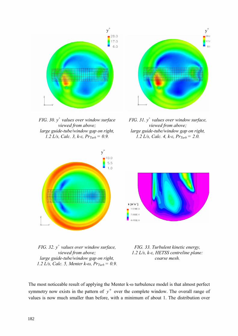
FIG. 30. y+ values over window surface viewed from above;

large guide-tube/window gap on right, 1.2 L/s, Calc. 3, k-ε, PrTurb = 0.9.

FIG. 31. y+ values over window surface, viewed from above;

large guide-tube/window gap on right, 1.2 L/s, Calc. 4, k-ε, PrTurb = 2.0.

FIG. 32. y+ values over window surface, viewed from above;

large guide-tube/window gap on right, 1.2 L/s, Calc. 5, Menter k-ω, PrTurb = 0.9.

FIG. 33. Turbulent kinetic energy, 1.2 L/s, k-ε, HETSS centreline plane:

coarse mesh.

The most noticeable result of applying the Menter k-ω turbulence model is that almost perfect symmetry now exists in the pattern of +y over the complete window. The overall range of values is now much smaller than before, with a minimum of about 1. The distribution over

y+ y+

y+

182

most of the strip ranges from 1 to about 6, but at the low-gap side it approaches the peak of 10, due to the higher velocity of the fluid passing over it. Plots of turbulent kinetic energy for calculations with different meshes, using the standard k-ε turbulence model and the standard value of 0.9 for PrTurb (Figs 33 to 35), show that there are large differences in the distributions in the region over the window.

FIG. 34. Turbulent kinetic energy, 1.2 L/s, k-ε, HETSS centreline plane:

intermediate mesh.

FIG. 35. Turbulent kinetic energy, 1.2 L/s, k-ε, HETSS centreline plane:

fine mesh.

Without further, detailed investigation of both the evaluation of +y in such regions of complex flows and geometry, as well as of the behaviour of numerical diffusion with these meshes, it is not possible to say more at this stage than to compare experimental and calculated temperature distributions. However, this is an area where further research study appears to be required.

4.1.4. Flow at the bottom of the target

The pattern of the flow field in close-up at the window is shown in Fig. 36, for the k-ε model, and Fig. 37, for the k-ω model, which can be compared qualitatively with the experimental results shown in Fig. 38, where all plots are in the plane through the maximum slant of the end of the guide tube. The maximum value of fluid velocity is almost the same for each turbulence model, but the detail of the flow distribution does differ. The profile across the annulus is more peaked with the k-ω model, giving slightly more penetration into the riser, at both sides of the guide tube. This leads to a longer recirculation region in the riser, above the small gap. On the window surface, on the other hand, the k-ε model causes a region of higher velocity inside the radius of the guide tube, at the small-gap side. This is detail that is not possible to see in the coarser distribution of experimental data. It is most likely the result of fluid penetrating from directions at right angles to the plane shown.

183

FIG. 36. Velocity vectors near the window, 1.2 L/s, k-ε, plane Z = 0 m:

fine mesh.

FIG. 37. Velocity vectors near the window, 1.2 L/s, k-ω, plane Z = 0 m:

fine mesh.

200 mm/s

FIG. 38. Experimental velocity vectors near the window, 1.2 L/s, plane Z = 0 m.

Due to the length of time it took to record the ultrasonic velocity measurements, the experimental grid matrix is relatively sparse compared with the CFD mesh distribution. However, there is good agreement in the vector field at the centre of the riser. The trends towards flow vortex production inside the edges of the guide tube are visible in the UVP results, but the instability and the high transverse gradients in these regions make it extremely difficult to resolve the field with the accuracy of these steady-state CFD results. Nevertheless, it can be concluded that there is quite good agreement between experiment and simulation, with CFX-4.4 being able to reproduce the flow field with no apparent problem.

From visual observation of the complexity of the flow under the edges of the guide tube, at the beginning of the HETSS strip, it appears necessary for the CFD mesh to be at least as fine as the finest mesh used here, in order to resolve the strong transverse velocity gradients and to model the momentum boundary layer accurately enough. As fluid passes from the annulus to the riser region, the flow expands and turns through 180°, generating a vortex of reversed flow up the inside of the guide tube, at the large-gap side (Fig. 39, for the fine mesh calculation).

184

FIG. 39. Velocity vectors in lower target, 1.2 L/s, k-ε, Z = 0 m, fine-mesh.

As far as the effect of the flow field on heat transfer at the HETSS strip is concerned, the tendency expected would be for the fluid velocity to be lower at the window surface under the largest gap, which would result in reduced heat transfer coefficient at this end of the strip, and hence higher wall temperatures. This would agree with the code predictions using the k-ε model, but not with the evidence from the experimental measurements, where there is inconclusive evidence that there is any significant change in heat transfer rate in this zone from that at the centre of the dome.

4.2. Flow-rate 3.6 L/s

With identical geometry and the same three degrees of mesh refinement, simulations were repeated with flow-rate in the target increased to 3.6 L/s, but only using the standard k-ε model (Table 7). The same trend of increasing accuracy of resolution in moving from the coarse to the fine mesh was observed as before, and consequently only the fine-mesh results will be looked at in detail here.

185

TABLE 7. MODEL MESHES AND TURBULENCE MODELS, 3.6 L/S FLOW-RATE

Calculation Mesh designation Total cells y+ range over

HETSS strip Turbulence model

7 A 239 256 30 → 210 Standard k-ε ( PrTurb = 0.9 )

8 B 336 120 20 → 110 Standard k-ε ( PrTurb = 0.9 )

9 C 451 800 12 → 76 Standard k-ε ( PrTurb = 0.9 )

4.2.1. Temperature distributions

Comparing the temperature distribution obtained using the k-ε model and the same mesh (Fig. 40) with that through the same vertical plane at the low flow-rate case (Fig. 17); it is immediately obvious that the hot boundary region next to the HETSS is significantly reduced in depth at higher flow-rate. There continues to be some penetration of hot fluid into the riser from the surface below the small gap, but the tongue of hot fluid has fully disappeared from under the large gap. This suggests that the increased velocity has caused fluid to reach further down to the HETSS surface in this region and cool the surface more efficiently, as well as dissipating heat more widely into the regions at the sides of the HETSS strip.

FIG. 40. Temperature contours, 3.6 L/s, plane Z = 0 m, k-ε model: fine mesh.

FIG. 41. Temperature contours, 3.6 L/s, window surface, k-ε model: fine mesh.

186

Comparison of Figs 41 and 21 shows that there remains a hotter zone on the HETSS strip under the large gap, but that it is smaller in extent and has been displaced to one side of the strip centreline, thus consequently having a smaller influence on the distribution shown in Fig. 40. What is also clear from Fig. 41 is that the peak that previously existed in surface temperature under the small gap has almost disappeared. The surface temperature alone is thus not responsible for the presence of the tongue of hot fluid into the riser. The higher fluid velocity in general has distorted the surface temperature distribution to a greater extent than at lower flow-rate, but with some swirl now visible in the opposite direction at the small-gap side, and with greater effect than before.

Averaged CFD temperatures, with all three-mesh models, and the HETSS experimental data are compared in Fig. 42. First of all, it is clear that the experimental distribution is both flatter than with a flow-rate of 1.2 L/s, is lower at the centre of the dome by some 33%, and now exhibits no significant peak under the small-gap edge of the guide tube. This latter could be expected from the increased penetration of fluid from the annulus into the bottom of the dome, creating more turbulence over the whole dome and smoothing out surface temperatures. What is significant about all of the CFD results, however, is that there continues to be a broad peak in temperature under the large gap, for all meshes, which the experimental data does not show.

Nevertheless, there remains a large difference between the window heat transfer obtained using the different meshes. The discrepancy using the coarse mesh continues to be very large, at both ends of the heated strip, and is of the order of 450%. The over-prediction ‘improves’ to a level of some 250% in the centre of the strip. However, the fine mesh again gives good agreement with the experiment over HETSS 1 to 8, and over HETSS 20 and 21. Between these zones a broad peak occurs, rising to about 55% at HETSS 15 and 16.

All the meshes generate this temperature rise, but the ramp is smoothest with the fine mesh. However, as the same HETSS strip was used as with the 1.2 L/s case, and the same effect occurred in this simulation (though to a lesser extent), it is possible that the HETSS units on this side could be inaccurate, but this would need further investigation of other test cases — which was beyond the scope of this present investigation.

0

5

10

15

20

25

30

0 1 2 3 4 5 6 7 8 9 10 11 12 13 14 15 16 17 18 19 20 21

Distance along HETSS strip [cm]

Tem

pera

ture

diff

eren

ce [º

C]

Finest mesh

Intermediate mesh

Coarse mesh

Experiment

HETSS 1

FIG. 42. Temperatures along HETSS strip, 3.6 L/s, k-ε turbulence model.

187

4.2.2. Boundary layer cell thickness: flow-rate 3.6 L/s

The validity of the application of the turbulence model can be assessed as before by looking at the values of +y calculated by the code. These are listed for the three cases in Tables 8 to 10.

TABLE 8. COMPARISON OF +y VALUES, 3.6 L/s FLOW, STANDARD k-ε TURBULENCE MODEL: COARSE MESH MODEL

Position A B C D

Wall cell thickness (mm) 6.59 2.89 3.04 5.87

+y (CFX-4.4) 96 45 (D side)

150 (C side)

82 101

+y (from (Eq.) 2) 254 196 251 258

TABLE 9. COMPARISON OF +y VALUES, 3.6 L/s FLOW, STANDARD k-ε TURBULENCE MODEL: INTERMEDIATE MESH MODEL

Position A B C D

Wall cell thickness (mm) 2.35 1.25 1.68 3.07

+y (CFX-4.4) 57 15 (D side)

35 (C side)

46 52

+y (from (Eq.) 2) 103 94 149 146

TABLE 10. COMPARISON OF +y VALUES, 3.6 L/s FLOW, STANDARD k-ε TURBULENCE MODEL: FINE MESH MODEL

Position A B C D

Wall cell thickness (mm) 1.40 0.75 0.69 1.33

+y (CFX-4.4) 30 15 (D side)

48 (C side)

25 16

+y (from (Eq). 2) 66 61 69 70

188

The poor performance of the coarse-mesh model is to be expected, as the +y values there (Table 8) are now well above the range of applicability for the momentum boundary layer, and the mesh is inadequate for picking up enough detail of the velocity profile at the window. The intermediate mesh appears to be just within the range of applicability for the k-ε model, but, with a higher flow-rate and subsequently thinner momentum boundary layer, again it is reasonable to assume that the mesh is not fine enough to adequately resolve the temperature profile through this layer.

The +y values with the fine mesh lie midway within the range of applicability of the turbulence model, and the temperature results confirm that this has led to the closest agreement with the experimental data. Nevertheless, the CFX-4.4 values for +y are between a factor of 2.8 and 4.4 lower than those from Eq. (2) at points C and D, respectively, at the ends of the HETSS strip.

A plot of +y over the inner surface of the window for Calculation 9, taken from the CFX-4.4 simulations with the standard k-ε model, is given in Fig. 43.

FIG. 43. y+ values over window surface, viewed from above; large guide-tube/window gap on right, 3.6 L/s ,Calc. 8, k-ε , PrTurb = 0.9.

The pattern of +y is very similar to that at the lower flow-rate and with the same mesh (Fig. 30), but with a rotational movement of about 60° in a clockwise direction when viewed from above. This rotation is most probably the result of the design of the inlet manifold system, and the difference in position has been caused by the higher velocity compared with the low flow-rate case. Values of +y have risen by a factor of 2 at the minimum and by 2.7 at the peak. The mean over the HETSS strip is now about 50.

y+

189

Examining the distribution of turbulent kinetic energy in the fine-mesh results (Fig. 44), and comparing with those for the low flow case (Fig. 35), it can be seen that the gradient of turbulent energy normal to the heated surface below the large gap is now much lower than at lower flow-rate.

The lowest turbulent energy level is higher by a factor of 2.4 than with the low flow, but is still lower by some 3 orders of magnitude than the maximum in this region. Nevertheless, the difference in the normal gradient at the wall under the large gap is a possible cause for the larger discrepancy between CFX-4.4 and Eq. (2) +y values in this region. The patterns of turbulent energy distribution under the small gap are similar for both flow-rates, which is consistent with the similar behaviour of the CFD heat transfer distribution in both cases.

FIG. 44. Turbulent kinetic energy, 3.6 L/s, plane Z = 0 m, k-ε model, fine mesh.

4.1.7. Velocity distributions: flow-rate 3.6 L/s

Comparison of velocity distribution shown in Fig. 45 with the distribution at low flow-rate, shown in Fig. 36, confirms that there is stronger unidirectional flow with the higher flow-rate over the lowest surface of the dome, in the plane of the HETSS strip. Previously, the flows from both ends of the slant generated two zones of near stagnation of the fluid – one a little right of centre near the bottom of the dome, and the second, smaller zone just inside a vertical line passing through the guide-tube wall at the smallest gap. Now only the stagnation zone near the smallest gap exists, and this is extremely small. However, the velocity over the wall is still low enough under the large gap that the heat transfer from wall to fluid could be reduced and the peak in the temperatures produced by the CFD code could be expected, though no temperature peak is seen in the experimental data.

There is a region of significantly higher velocity at the surface, to the right of the small gap, compared with the velocity pattern with the lower flow-rate of 1.2 L/s, and this is the most likely cause of the elimination of the peak in the CFD calculations in this region (and would also be expected to be the reason for the same result in the experiment).

190

FIG. 45. Velocity vectors, 3.6 L/s, plane Z = 0 m, k-ε model, fine mesh.

5. CONCLUSIONS

5.1. Flow-rate 1.2 L/s

(1) The mesh must be refined sufficiently to give +y values close to the lower limit for applicability for the standard k-ε turbulence model. This both improves convergence and gives most accurate results for heat transfer between fluid and wall.

(2) The standard k-ε model gives closer agreement with the experimental temperature data than the Menter-modified k-ω model (using the same mesh), although the influence of even finer mesh cells in the fluid next to the wall with this latter model was not tested.

(3) Trends in variation of heat transfer over the surface of the window from the annulus to the target centreline were amplified in the CFD simulation, with the k-ε model, but it has not been possible to confirm if the effect is damped in the experiment in some way, as CFD results show a symmetry that is logical, whereas the experimental data shows some asymmetry. This could point to a lack of sensitivity of the HETSS at the large-gap end of the instrumented strip. But this limited data is insufficient to prove if this is really the case, or not.

(4) There is quite good qualitative agreement between experimental and CFD-generated velocity vector patterns in the centre of the window region of the test-section, though less good elsewhere. However, more extensive analysis of this and other tests is necessary in order to be able to accurately assess the agreement of measurement and prediction.

5.2. Flowrate 3.6 L/s

(1) Using the standard k-ε model and the same fine mesh as for the 1.2 L/s case also showed the best agreement with experiment, and this agreement was good at the beginning of heating, on both sides, and in the region under the smallest gap below the edge of the guide tube.

(2) A decrease in heat transfer under the larger gap, and from this region over the centre of the window, was present in the CFD simulation but not repeated in the experiment. This could also indicate a lack of sensitivity of the HETSS in this zone to the fluid flow, as noted for the lower flow-rate case, but would need further comparison, with data from different tests, before any firm conclusions can be made.

191

REFERENCES

[1] PLATNIEKS, I., BAUER, G.S., LIELAUSIS, O., TAKEDA, Y., Measurements of Heat Transfer at the Beam Window in a Mockup Target for SINQ Using Mercury, Proc. 14th Meeting of the International Collaboration on Advanced Neutron Sources, (ICANS XIV), Starved Rock Lodge, Argonne National Laboratory (1998) pp. 382–395.

[2] PLATNIEKS, I., BAUER, G.S., LIELAUSIS, O., TAKEDA, Y., Measurements of Heat Transfer at the Beam Window in a Mockup Target for SINQ Using Mercury, Proc. 14th Meeting of the International Collaboration on Advanced Neutron Sources (ICANS XIV), Starved Rock Lodge, Argonne National Laboratory (1998) pp. 382–395.

[3] TAKEDA, Y., Velocity profile measurement by ultrasonic Doppler method, Exp. Therm. & Fluid Sci., Vol. 10 (1995) pp. 444–453.

[4] VARGAFTIK, N.B., Handbook of Physical Properties of Liquids and Gases, Pure Substances and Mixtures, Springer-Verlag, Berlin, ISBN 3-540-16972-5 (1983).

[5] TAKEDA, Y., KIKURA, H., Measurement of Mercury Flow by Ultrasonic Doppler Method, Proc. FEDSM’98, FEDSM98-5074, ASME Fluids Engineering Division Summer Meeting, 21–25 June1998, Washington, DC, USA (1998).

[6] CFX-4.3, User Documentation Volume 3: Solver (Part 1), AEA Technology, Harwell, Oxford, UK (1999) pp. 3-180–3-182.

[7] CASEY, M., WINTERGERSTE, T., (Eds), Special Interest Group on Quality and Trust in Industrial CFD, Best Practice Guidelines, ERCOFTAC, Version 1.0, Fluid Dynamics Laboratory, Sulzer Innotec, Winterthur, Switzerland (2000).

[8] SMITH, B.L., On Boundary Layer Modelling Using the ASTEC Code, PSI Bericht Nr. 101, Paul Scherrer Institute, Switzerland (1991) p. 16.

[9] CFX-4.3, User Documentation Volume 3: Solver (Part 2), AEA Technology, Harwell, Oxford, UK (1999) pp. 3-685–3-686.

[10] VIESER, W., ESCH, T., MENTER, F., Heat Transfer Predictions using Advanced Two Equation Turbulence Models, CFX Technical Memorandum CFX-VAL10/0602 (May 2002).

[11] WILCOX, D.C., Turbulence Modelling for CFD, DCW Industries, Inc., La Canada, CA (1993).

192

SESSION 2

REVIEW OF CURRENT AND PLANNED EXPERIMENTAL HLM PROGRAMS

THERMAL HYDRAULIC RESEARCH AND DEVELOPMENT NEEDS FOR LEAD FAST REACTORS

J.J. SIENICKI, D.C. WADE, C.P. TZANOS Argonne National Laboratory, Argonne, Illinois, United States of America

Abstract

Lead-cooled fast reactors (LFRs) have the potential to meet the future needs of developed and developing nations for proliferation resistant, passively safe, autonomous, modular battery plants that provide electricity or hydrogen and potable water. The Secure Transportable Autonomous Reactor (STAR) project at Argonne National Laboratory has developed 400 MWt reactor concepts cooled by molten lead. In the course of work on the concepts, extensive research and development needs have been identified. Thermal hydraulic R&D needs have been identified in the areas of: Pb temperatures and velocities in large open-lattice cores; stability of autonomous power-driven natural circulation; flow stratification and other 3-D effects with natural circulation during operational transients and postulated accidents; transient void and coolant dynamics and interactions following heat exchanger (HX) tube rupture, startup strategy and 3-D thermal hydraulic conditions during startup; HX thermal hydraulics; removal of reactor afterheat; fundament heat transfer tests; and supercritical CO2 Brayton cycle power conversion.

1. INTRODUCTION

Lead-cooled fast reactors (LFRs) have the potential to meet the future needs of developed and developing nations for proliferation resistant, passively safe, autonomous, modular battery plants that provide electricity or hydrogen and potable water. The Secure Transportable Autonomous Reactor (STAR) project at Argonne National Laboratory has developed 400 MWt reactor concepts cooled by molten Pb-lead: STAR-LM (Liquid Metal) for production of electricity utilizing a gas turbine Brayton cycle with supercritical carbon dioxide (S-CO2) as the working fluid, and potable water production using reject heat; and STAR-H2 for hydrogen generation via thermochemical water cracking, and water production. In the course of work on the concepts, extensive research and development (R&D) needs have been identified. This paper discusses those specific R&D needs that relate to the thermal hydraulics of the lead primary coolant system and the S-CO2 balance of plant.

2. OVERVIEW OF STAR-LM DESIGN FEATURES

STAR-LM is a 400 MWt proliferation resistant, modular, factory-fabricated, fully transportable, autonomous load following, and passively safe lead-cooled fast reactor [1–6] (see Fig. 1 and Tables 1 and 2).

Recent development of STAR-LM has replaced the traditional Rankine steam cycle with a gas turbine recompression Brayton cycle that utilizes supercritical carbon dioxide (S-CO2) as the working fluid [7–9].

Consistent with the higher operating temperatures of the S-CO2 Brayton cycle, Pb (Tmelt = 327 ΕC; Tboil = 1740 ΕC) has been selected at the primary coolant. Lead is less corrosive to unprotected steel than lead-bismuth eutectic (LBE) and has a two to three orders of magnitude lower activity from formation of Po210. The STAR-H2 reactor system is similar but operates at higher temperatures required for water cracking.

195

FIG. 1. Illustration of STAR-LM reactor.

196

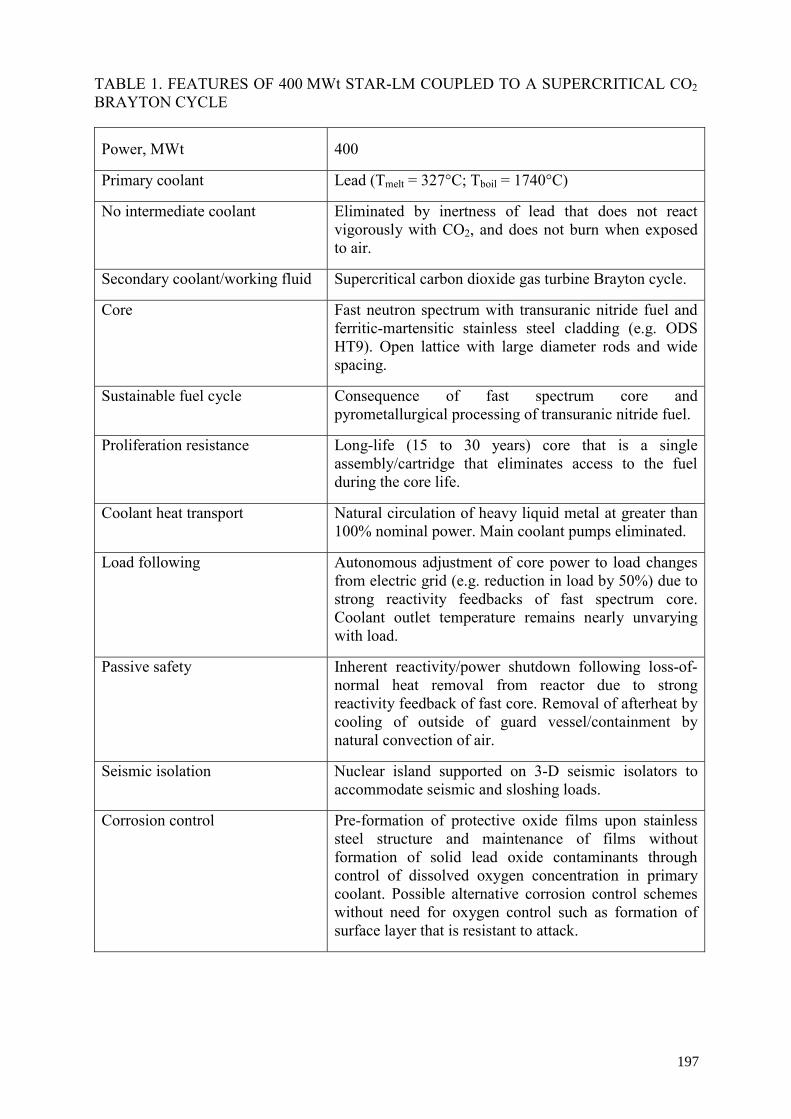
TABLE 1. FEATURES OF 400 MWt STAR-LM COUPLED TO A SUPERCRITICAL CO2 BRAYTON CYCLE

Power, MWt 400

Primary coolant Lead (Tmelt = 327°C; Tboil = 1740°C)

No intermediate coolant Eliminated by inertness of lead that does not react vigorously with CO2, and does not burn when exposed to air.

Secondary coolant/working fluid Supercritical carbon dioxide gas turbine Brayton cycle.

Core Fast neutron spectrum with transuranic nitride fuel and ferritic-martensitic stainless steel cladding (e.g. ODS HT9). Open lattice with large diameter rods and wide spacing.

Sustainable fuel cycle Consequence of fast spectrum core and pyrometallurgical processing of transuranic nitride fuel.

Proliferation resistance Long-life (15 to 30 years) core that is a single assembly/cartridge that eliminates access to the fuel during the core life.

Coolant heat transport Natural circulation of heavy liquid metal at greater than 100% nominal power. Main coolant pumps eliminated.

Load following Autonomous adjustment of core power to load changes from electric grid (e.g. reduction in load by 50%) due to strong reactivity feedbacks of fast spectrum core. Coolant outlet temperature remains nearly unvarying with load.

Passive safety Inherent reactivity/power shutdown following loss-of-normal heat removal from reactor due to strong reactivity feedback of fast core. Removal of afterheat by cooling of outside of guard vessel/containment by natural convection of air.

Seismic isolation Nuclear island supported on 3-D seismic isolators to accommodate seismic and sloshing loads.

Corrosion control Pre-formation of protective oxide films upon stainless steel structure and maintenance of films without formation of solid lead oxide contaminants through control of dissolved oxygen concentration in primary coolant. Possible alternative corrosion control schemes without need for oxygen control such as formation of surface layer that is resistant to attack.

197

TABLE 2. DESIGN AND OPERATING CONDITIONS OF 400 MWt STAR-LM COUPLED TO A SUPERCRITICAL CARBON DIOXIDE BRAYTON CYCLE

Core thermal power, MWt 400

Coolant Pb

Core diameter, m 2.41

Core active (heated) zone height, m 2.0

Fission gas plenum height, m 0.5

Fuel rod cladding outer diameter, cm 1.91

Fuel rod triangular pitch-to-diameter ratio 1.50

Core hydraulic diameter, cm 2.82

Cladding thickness, mm 1.0

Transuranic fuel outer diameter, cm 1.51

Transuranic fuel smeared density 0.78

Number of grid spacers 3

Secondary coolant Supercritical

CO2

Height difference between heat exchanger (HX) and core thermal centers, m

7.53

Height difference between top of HX tubes and bottom of core, m 12.0

HX tube height, m 6.94

HX inner diameter, m 2.98

HX outer diameter, m 5.14

HX tube inner diameter, cm 1.0

HX tube outer diameter, cm 1.4

HX tube triangular pitch-to-diameter ratio 1.6

HX primary coolant hydraulic diameter, cm 2.55

Total number of HX tubes in all HXs 25 500

Fuel doppler reactivity feedback coefficient, cents/°C -0.153

Fuel and cladding axial expansion reactivity feedback coefficient, cents/°C

-0.05384

Coolant density reactivity feedback coefficient, cents/°C 0.1489

Core radial expansion reactivity feedback coefficient, cents/°C -0.5484

198

Ctd’

Enhancement of core radial expansion relative to grid spacer thermal expansion

4.0

Core coolant inlet temperature, °C 420

Core coolant outlet temperature, °C 560

Mean temperature rise through core, °C 140

Peak cladding outer surface temperature, °C 632

Peak cladding inner surface temperature, °C 650

Peak fuel centerline temperature, °C 773

Pb coolant mass flowrate, kg/s 19 700

Mean Pb coolant velocity in core, m/s 0.697

Mean Pb coolant density, kg/m3 10 440

Supercritical CO2 pressure at top of HX, MPa 19.9

CO2 Temperature at bottom of HX, °C 392

CO2 Temperature at top of HX, °C 545

CO2 Mass flowrate, kg/s 2 100

Total CO2 circulating inventory, kg 32 900

Brayton cycle efficiency, % 44.2

Plant efficiency, % 43.8

The STAR-LM concept takes advantage of the benefits of inert lead coolant to eliminate the need for an intermediate heat transport circuit. In addition, 100+ % of the core full power is transferred by natural circulation from a low power density/low pressure drop core, which is located at the bottom of the reactor vessel, to in-vessel modular heat exchangers (HXs) at the top of the vessel.

The HXs are in the outer annular region between an above-core cylindrical shroud and a cylindrical liner situated immediately inside of the vessel. Natural circulation heat transport eliminates the need for main circulation pumps and thereby eliminates the entire class of accidents associated with the loss of forced flow. The core and HX thermal centers are separated by a distance of 7.5 m.

The core utilizes a fast neutron spectrum with transuranic nitride fuel and ferritic-martensitic stainless steel cladding combined with pyrometallurgical reprocessing thus providing for a sustainable fuel cycle. Nitride fuel has a high melting temperature and high thermal conductivity, and offers the prospect of low release of fission gas. The open lattice, low-power density core has an extremely long refueling interval of 15 years or longer. In addition, the core is designed as a single large assembly/cartridge that is not composed of individual removable fuel assemblies.

199

The long core lifetime, coupled with the single assembly design, eliminates access to the fuel during the core life thereby contributing to proliferation resistance. Large diameter (e.g. 1.9 cm OD) fuel rods are arranged on a square or triangular pitch of large spacing (triangular p/d = 1.5); separation is maintained by grid spacers similar to a LWR fuel bundle. The open-lattice core eliminates the entire class of accidents associated with the blockage of a fuel assembly. The core active (heated) height is 2.0 m. Strong radial and axial power profiles (Ppeak/Pavg ~1.7) combined with low natural circulation velocities (~0.7 m/s) result in strong temperature and velocity variations across the core.

For STAR-LM, corrosion control of the stainless steel structures may be achieved through the Russian-based approach of pre-formation of a protective Fe3O4 layer upon the steel structure and maintenance of the layer through control of the dissolved oxygen level in the lead coolant. The oxygen concentration is actively controlled at a level above that required for the formation of the Fe3O4 protective oxide films upon the structures while avoiding the buildup of solid PbO oxide contaminant in the coolant. Alternative corrosion control schemes are also under investigation for STAR-LM and STAR-H2; development of an alternative approach is essential for the higher temperatures at which STAR-H2 operates (e.g. Tinlet ~650°C; Toutlet ~800°C). Usage of SiC and SiC composites is being investigated. The reactor is situated below grade inside of a silo (see Fig. 1) enhancing the resistance to the effects of an aircraft crash; if needed, the depth of the silo can be further increased. A nuclear island is supported on three-dimensional seismic isolators to accommodate seismic and sloshing loads in regions of significant seismicity. Startup and shutdown are implemented through removal/insertion of shutdown rods. In the case of initial startup, the system must be externally heated and a suitable initial flow pattern established prior to the initiation of fission power.

Recent development of STAR-LM has coupled the reactor to an advanced power conversion system that incorporates a gas turbine Brayton cycle utilizing supercritical carbon dioxide (S-CO2) as the working fluid. Figure 2 shows a schematic illustration of STAR-LM coupled to its S-CO2 Brayton cycle. The S-CO2 Brayton cycle offers significantly improved cycle efficiency relative to a traditional Rankine water/steam cycle; an efficiency of 44% is calculated for the nominal operating condition of Fig. 2. The plant footprint is reduced due to fewer, simpler, and smaller-sized components. This offers the prospect of reduced capital and operating costs as well as reduced plant staffing requirements from radical plant simplification and elimination of costly Rankine cycle components. In particular, the turbine and compressors optimally designed for the STAR-LM 400 MWt cycle conditions have a remarkably small size due to the high S-CO2 density (468 kg/m3 at the critical point). The four-stage turbine has a length of only 0.8 m and diameter of 1.25 m without the casing.

The strong reactivity feedback from the fast neutron spectrum core enables autonomous load following whereby the reactor power adjusts itself to match heat removal from the primary coolant solely as a consequence of inherent physical processes. Brayton cycle conditions are altered during load following by means of a control scheme that seeks to maintain unvarying maximum and minimum S-CO2 pressures (i.e. 20 and 7.4 MPa) as well as unvarying turbine and compressor shaft speeds (3 600 rpm). The scheme is implemented by:

200

(i) venting S-CO2 from the circuit to a reservoir/tank should the maximum pressure exceed a setpoint or the turbine shaft speed exceed a setpoint; and

(ii) adding S-CO2 to the circuit from the reservoir should the minimum pressure fall below a setpoint or either compressor shaft exceed a setpoint.

The system temperatures that are attained following an autonomous power change from the nominal steady state can be optimized through design of the core clamping and restraint approach to enhance the negative reactivity feedback from core radial expansion/flowering. In particular, an approximately unvarying core outlet temperature can be achieved; this results in an approximately unvarying maximum temperature to which the S-CO2 is heated and, hence, an approximately unvarying Brayton cycle efficiency during load following.

100 % Power

545.5 269.9 175.3CO2 19.91 2103 Kg/s 422.8

7.502392.119.98

Pb 176.11 atm Eff = 44.3 % 20559.6 396 178.7

T, C T,C 20 178.7Air Q,MW P,MPa 7.451RVACS 174.7

420 4 48.9 20Avg

421.4 Hot400 Coolnt

703.7 629.4 603.3 589.3 559.6 31.25 84.2 85773.3 682.6 650.0 632.3 594.3 7.4 20.00 7.405

420.0 420.0 742.3 610.7 564.3 539.5 489.8820.0 659.4 601.4 570.3 507.1 39

19727 Kg/s 564.2 485.4 459.7 445.8 420.0599.0 501.7 469.5 452.3 420.0 65%

Tcl Tfo Tci Tco Tc 35%

CORE

STAR-LM TEMPERATURES AND PRESSURES

In

Fuel Cladding

Out

Mid

TURBINEHTR

CORE

RHX

COOLANT MODULE VESSEL

LTR

COMP. #1

COMP. #2

COOLER

FIG. 2. Thermal hydraulic conditions for STAR-LM coupled to S-CO2 Brayton cycle.

201

As a consequence of the reactivity feedback, the core power passively decreases to low power levels typical of decay heat levels, in the event of an accident such as the complete loss of normal heat removal through the in-reactor heat exchangers. The reactor afterheat is passively removed by the Reactor Exterior Cooling System that cools the outside of the containment/guard vessel by the natural convection of air flowing upwards over the vessel. This concept is illustrated in Fig. 1.

3. RESEARCH AND DEVELOPMENT NEEDS

3.1. Open-lattice core thermal hydraulics

The LFR core is refueled at the factory at long-term (15 to 30 year) intervals. Therefore, the core is not composed of individual removable fuel assemblies but is a single large cassette/assembly. Elimination of the need for removable fuel assemblies eliminates the need for flow ducts/hexcans that had been a feature of traditional sodium-cooled fast reactors (SFRs). The absence of fuel assembly ducts allows for cross-flows and eliminates potential events involving blockage of a single assembly. Because of the relatively low power density (relative to traditional SFRs) as well as the high nitride fuel density, the core can be designed as a single large assembly of large diameter fuel rods laid out as a square or triangular lattice having a large pitch-to-diameter ratio. The resulting large hydraulic diameter reduces the core pressure drop and enables natural circulation heat transport of more than 100 percent of the full core power. Grid spacers support the fuel rods similar to a Western design pressurized water reactor (square lattice) or Soviet-designed VVER reactor (triangular lattice).

The velocities through the core from natural circulation are low (e.g. umean ~0.7 meter per second) relative to a forced flow system. A LFR core design can have a significant power spatial distribution (Ppeak/Pavg = 1.7) that gives rise to significant temperature and velocity profiles across the core. The temperature field induces buoyancy effects that drive significant cross-flows between the channels giving rise to coolant intermixing. In addition, intermixing of the lead liquid metal coolant is enhanced by liquid metal turbulent transport.

The importance of the cross-flows and turbulent transport is made even greater by the relatively low coolant axial velocities. Crossflow and intermixing are important because they reduce the value of the peak cladding temperature for a fixed core outlet temperature. The peak cladding temperature is related to the potential for oxide layer growth/penetration into the cladding material over the core lifetime, for corrosion control based upon pre-formation of a Fe3O4 layer and active control of the oxygen potential in the lead. Grid spacers may be an effective means of further reducing the peak cladding temperatures through enhancement of coolant intermixing.

Scoping calculations were carried out of the velocities and temperatures across the STAR-LM core using the porous medium model of the STAR-CD computational fluid dynamics code [10]. A three-dimensional hexagonal prismatic nodalization of a one-twelfth core segment was employed; this nodalization corresponds to the three-dimensional power distribution obtained from a DIF3D neutronics calculation. The k-, model for turbulent transport was employed. Grid spacers were not modeled. The flow boundary condition at the bottom of the active core inlet was different from that corresponding to the velocity in Table 2.

Figures 3 and 4 show the calculated velocity and temperature distributions at the top of the 2 meter active core at the beginning of life. Significant velocity and temperature profiles are

202

calculated by the scoping analysis. The temperature at the top of the hot channel in the active core exceeds the core outlet temperature by 32 ΕC versus 37 ΕC calculated by a one-dimensional hot channel analysis without intermixing due to cross-flow and turbulent transport and without channel-to-channel thermal conduction.

Because of the large channel hydraulic diameter, entrance effects can encompass a significant fraction of the active core height. A scoping analysis of the hot channel at beginning-of-life was carried out using STAR-CD [10].

The low-Re number k-, model was employed with an adaptive mesh in which the mesh size in the radial direction from the fuel rod grows by a ratio of about 1.2. One-sixth of the channel surrounding the rod over the 2 meter active core height was simulated with 660 000 computational cells. Figure 5 shows the calculated heat transfer coefficient. The calculated entrance effect is observed to extend over half of the active core height. More detailed STAR-CD analyses of cross-flow and intermixing are underway. Research and development needs include the development of a reliable code capability to calculate three-dimensional thermal hydraulic conditions in open lattice rod arrays that incorporate grid spacers or other support or heat transfer enhancement structures. Experiments need to be designed and conducted to obtain definitive thermal hydraulic data with prototypic rod arrays having a prototypic height. Experiments should include tests with significant power distributions across the rod array. The effects of grid spacers upon coolant intermixing, frictional pressure drop, and heat transfer need to be measured. Specific tests should be performed with and without grid spacers. Data obtained must meet the requirements for validation of multidimensional thermal hydraulic computer codes including the measurement of local temperatures and velocities.

FIG. 3. Velocity distribution at the top of the active core at beginning of life.

PROSTAR 3.10

COMPONENT W

M/S

LOCAL MX= 0.4861

LOCAL MN= 0.3099

0.4861

0.4735

0.4609

0.4483

0.4357

0.4232

0.4106

0.3980

0.3854

0.3728

0.3602

0.3476

0.3351

0.3225

0.3099

203

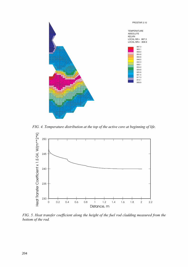
FIG. 4. Temperature distribution at the top of the active core at beginning of life.

0 0.2 0.4 0.6 0.8 1 1.2 1.4 1.6 1.8 2 2.2

Distance, m

230

235

240

245

250

He

atTr

ansfe

rC

oe

ffic

ientx

1.E

-04

,W

/(m

**2

*K)

FIG. 5. Heat transfer coefficient along the height of the fuel rod cladding measured from the bottom of the rod.

PROSTAR 3.10

TEMPERATURE

ABSOLUTE

KELVIN

LOCAL MX= 867.3

LOCAL MN= 808.9

867.3

863.1

859.0

854.8

850.6

846.5

842.3

838.1

834.0

829.8

825.6

821.5

817.3

813.1

808.9

204

3.2. Stability of autonomous power-driven natural circulation

The LFR fast spectrum core has strong reactivity feedbacks to changes in the coolant and fuel temperatures that enable autonomous changes in power in response to changes in load demand/heat removal. However, the coolant flow-rate as well as the temperature rise through the core (and, hence, the core coolant temperatures) are directly dependent upon the reactor power. Thus, a perturbation in coolant flow or temperature can cause a perturbation in the core power that, in turn, affects the fuel temperatures, coolant temperatures, and coolant flow-rate. Crucial questions therefore concern the potential for development of oscillations in power, system temperatures, and flow, and whether small perturbations in power, temperature, or flow can grow to significant magnitude. The desired behavior is for oscillations that may be caused by perturbations to rapidly decay away. The potential for oscillations and perturbation growth may be depend upon the reactor core power level or the natural circulation flow-rate. One-dimensional linear perturbation analyses have been formulated for the simpler case of fixed core power [11, 12]. The analyses can delineate the stability boundaries for forwards and backwards natural circulation. Extension to an autonomous power core is in progress. Research and development needs include analyses that determine the regimes of design conditions under which reactivity feedback results in the calculation of unstable behavior over the spectrum of possible power and flow conditions. It may turn out that the unstable regimes are far removed from the actual reactor design conditions. The purpose is to determine which design features may have the potential to result in instabilities so that they may be avoided by the designer.

Experiments need to be carried out to investigate the conditions under which natural circulation can become unstable when the heat source power depends upon the system temperatures. This could be achieved through computer control of the power source for the experiment (e.g. electrically heated fuel rod simulators) in response to on-line measurement of system temperatures. The data is needed to test and validate analysis methodologies employed to delineate regimes of stability. Experiments need to be able to establish both forwards and backwards flow configurations.

3.3. Stratification and other 3-D effects with natural circulation during operational transients and postulated accidents

One-dimensional first principles analyses provide a relationship between the steady state coolant flow-rate and core power, as well as between coolant temperature rise and core power. Experiments with heavy liquid metals are needed to determine the applicability of the steady state relationship over a range of power/flow under conditions where multidimensional effects are present. As discussed above, the strong power profile across the core gives rise to significant temperature and velocity profiles across the core. Thus, temperature and velocity profile effects should be present inside the simulated core and heat exchangers(s). This can be accomplished by simulating a core with a number of electrically heated fuel rod simulators and with a heat exchanger that incorporates a number of tubes. At low power levels, profile effects are expected to become more pronounced.

An example of an operational transient is a change in load/heat removal from the reactor. An example of an accident is the loss of normal heat removal through the heat exchangers. In operational transients and postulated accidents, multidimensional effects can occur such as flow stratification inside the reactor vessel lower plenum or the above-core riser; or where reverse/downward flow might conceivably occur through lower power portions of the core during a fast startup/rise in power from a shutdown condition.

205

A transient analysis code capability is required that incorporates the calculation of three dimensional effects including stratification but yet can be run efficiently with a short turnaround time. Experiment data are needed from a facility that can simulate the phenomena that occur during operational transients and postulated accidents. The multidimensional phenomena can be encompassed experimentally through the use of a tall vessel that incorporates models of the core, above-core shroud, heat exchanger(s), downcomer, and below-core flow distribution structure. A one-dimensional loop that is constructed out of piping is inadequate because it would exclude the multidimensional effects.

3.4. Transient void and coolant dynamics following heat exchanger tube rupture

In the case of CO2, chemical equilibrium calculations predict the absence of interaction between Pb and CO2 above about 250 ΕC which is well below the lead melting temperature. Thus, no reaction is expected between molten lead and CO2. However, when either a supercritical carbon dioxide Brayton cycle or Rankine steam cycle is utilized for the secondary side, the secondary coolant exists at much higher pressure than the low pressure lead or lead-bismuth eutectic (LBE) primary coolant. Failure of the lead-to-secondary coolant interfacing boundary inside an in-reactor heat exchanger will result in a high pressure blowdown of secondary coolant into the lead. Possible consequences include the transient growth of void inside the primary coolant and the potential, in some designs, for transport of void into the core region that might result in reactivity/power increase and degradation of core-to-coolant heat transfer. The consequences of void formation and transport into the core are dependent upon design features of the reactor system and the heat exchangers; the potential for void transport to the core can be significantly reduced or eliminated altogether by means of deliberate design measures. STAR-LM incorporates a pressure relief system for the reactor vessel and upper head/cover. A liner (i.e., a cylinder) is located interior to the reactor vessel inside surface. During operation, the lead coolant level inside the vessel-liner gap is below the top of the liner. The gap provides an escape path for CO2 to benignly rise to the lead free surface/cover gas region.

Thus transient dynamics of void growth and transport following rupture of a 1 cm inner diameter tube of the reference HX design was analyzed [13]. Growth of the large bubble was calculated with a one-dimensional equation for the bubble radius. It was determined that the blowdown involves the formation of large gas bubbles that penetrate minimally downwards into the lead coolant below the HX; a key feature is the heavy coolant density that retards bubble growth. Thus, it is concluded that the CO2 escapes to the free surface through the vessel-liner gap. Taylor instabilities at the surface of the growing large bubble result in intermixing of void and lead to form small bubbles. However, the fraction of CO2 intermixed with the lead by this process is calculated to be small (less than 3%) and the small bubbles formed to be of large diameters (d > 0.7cm) such that the terminal rise velocity exceeds the lead down-flow velocity beneath the HX. Thus, the smaller bubbles are not predicted for transportation through the core; they also rise benignly to the free surface.

An experiment facility needs to be designed and constructed to conduct experiments that simulate processes involved with CO2 and steam blowdown in lead and lead-bismuth eutectic coolants. It should be possible to simulate failure of a single tube to experimentally determine the transient void growth, breakup, and escape to the free surface as well as the chemical reaction products and the extents of their formation. Data is also needed to test and validate analysis methodologies.

206

3.5. Startup strategy and 3-D thermal hydraulic conditions during startup

During nominal operation, a LFR may operate autonomously with the primary coolant flow-rate driven solely by natural circulation. In ideal autonomous operation, the burnup-induced reactivity swing is small such that the requirement to compensate the associated reactivity change with control rods may be absent or small. Prior to startup and fission power production, power must be supplied by other means to maintain the coolant in a molten state and to establish a suitable flow pattern for transition to the desired natural circulation flow with fission heating. To initiate fission power, and to bring the reactor to nominal power, it is necessary to add significant reactivity to the core. This can be accomplished through the withdrawal of a safety rod or set of rods that take the reactor from deeply subcritical to near critical. Finer reactivity control is then required to encompass uncertainties in the additional reactivity needed to bring the core to criticality, and to raise the power to the desired level.

Sufficient heating of the reactor must be provided to compensate for heat losses. Heat may be carried away by natural convection of air flowing over the outside of the containment/guard vessel or the containment/reactor vessel cover/upper head. External heating of the containment vessel could be provided using heated air to raise the temperature of the lead coolant and reactor internal structures, and to compensate for heat losses. However, this could result in a reverse flow pattern in which heated lead flows upwards along the inside of the reactor vessel and downwards through the core. The flow direction could be changed to the desired one with upward flow through the core by one of a number of means. One could be to inject coolant downwards over the reactor vessel inner surface at a rate that is sufficient to overcome the effects of buoyancy induced by the externally heated wall. This capability could be part of an active system to control the concentration of dissolved oxygen in the coolant. To maintain a proper coolant level, lead would be withdrawn from the reactor. A second approach could be to include a propeller, say above the core, to establish upwards flow through the core. A third approach would be to temporarily inject non-condensable gas above the core (i.e. a lift pump) to drive the flow in the proper direction due to density differences between single-phase liquid in the heat exchanger and downcomer versus two-phase coolant above the core. A fourth approach could be to incorporate jet pumps into the primary circuit. A jet pump maintains an open configuration for flow and would therefore have a small effect upon natural circulation heat transport. After a flow-rate upwards through the core of sufficient size is established, then the reactor would be brought to criticality and power. The method used to provide flow assist (e.g. a lift pump) would then be terminated, as the coolant flow-rate from single-phase natural circulation alone transports energy from the core to the in-reactor heat exchangers.

Little work has been done to determine the size of the assisted flow-rate that would be required during startup of a natural circulation LFR. The steady state coolant flow-rate in natural circulation depends approximately upon the cube root of the core power. Thus, at 0.1% nominal power, the flow-rate is about one-tenth the nominal steady state value. Consequently, the flow-rate required to bring the reactor to even a small fraction of nominal power could be a significant fraction (e.g. tenths) of the nominal flow-rate.

The power profiles that have been calculated for LFR cores reveal a high peak-to-average ratio. Without assisted flow, it might be expected that a sudden increase in power might temporarily result in enhanced upwards flow in the higher power regions of the core and reduced or even downwards flow in the lower power regions. However, a multidimensional transient analysis remains to be undertaken. This raises the question of how large the assisted flow-rate would need to be to avoid significantly reduced or downwards flow through the core during a rapid startup or increase in power.

207

Thus, a research and development need involves the transient multidimensional velocities and temperatures within the core that result from a rate of increase in power. The R&D needs include determination of the assisted flow-rate that precludes the possible development of adverse multidimensional flow and temperature effects. The needs are obviously related to the needs of open-lattice core thermal hydraulics discussed above but also involve the calculation of transients. Thus, a multidimensional code capability is needed that can be run with short turnaround time. Design analyses of lift pump systems are needed to determine the regime of non-condensable gas injection rate that produces the desired flow-rate without gas entrainment throughout the circuit. Experiments are needed to validate lift pump modeling for gas injection into heavy liquid metal coolants. Operating regimes that avoid gas void entrainment throughout the circuit need to be determined.

3.6. Heat exchanger thermal hydraulics

The LFR is coupled to the S-CO2 Brayton cycle through modular lead-to-S-CO2 heat exchangers (HXs) immersed inside the lead primary coolant. The HXs must fit within the available space in the reactor vessel and must also efficiently heat the S-CO2 to a sufficiently high temperature, in order to achieve the desired high Brayton cycle efficiency. For the 400 MWt STAR-LM, the design of shell-and-tube HXs that meet the requirements is feasible but there is a definite benefit to the cycle efficiency if heat transfer could be enhanced by means of surface protrusions [14–16] on the tubes. A HX would be designed to attempt to achieve one-dimensional downwards flow of lead over the exterior of the tubes inside which S-CO2 flows upwards. Grid spacers may also be utilized to support the tubes and enhance intermixing of the lead coolant. However, multidimensional flow effects are unavoidable and will decrease the HX effectiveness.

Research and development needs include multidimensional code calculations of lead and S-CO2 velocities and temperatures within the HX as well as the S-CO2 mean outlet temperature. Experiments are needed that simulate the HX configuration with a number of tubes. Data is required for validation of multidimensional thermal hydraulic codes.

3.7. Removal of reactor afterheat

In the event of complete loss of normal heat removal through the in-reactor heat exchangers that are immersed in the lead coolant, the reactor afterheat must be removed by passive means. An attractive approach is passive cooling of the exterior of the containment/guard vessel by natural convection of air. Reactor vessel air cooling has been selected for the STAR-LM LFR concept. It was found necessary to enhance the heat transfer rate above that corresponding to an unmodified vessel surface finish. One approach is to provide surface protrusions/projections that enhance turbulent transport of energy from the wall to air. A relatively low cost means of providing protrusions is to weld a bead around the circumference of the vessel at successive heights. This approach was identified for the PRISM SFR. While the approach increases the effective wall-to-air heat transfer coefficient, the enhancement did not remain sufficient as the power level of the PRISM series was increased. For the Super-PRISM design variant, a perforated collector cylinder is also installed inside the channel for upwards flow of air over the containment vessel. The perforated collector catches part of the thermal radiation emitted by the vessel and heats up; energy is transferred to air from the heated collector by turbulent forced convection. The circular hole perforations enable thermal radiation to also heat the far wall of the annular air channel for upwards flow from which additional energy is transferred to air by forced convection. The net effect is an increase in surface area for forced convection heating of the air. Other configurations to enhance energy transfer may be devised. Typically, a gap exists between the reactor vessel and the

208

surrounding containment/guard vessel. A gap enables ultrasonic examination of the reactor vessel wall to be carried out. Inspectability of the reactor vessel is a code requirement. Elimination of the gap is, therefore, not practical. In earlier liquid metal reactor designs, the gap was filled with a non-condensable gas. Due to the low gas thermal conductivity, removal of the reactor afterheat was limited by thermal radiation from one vessel surface to the other across the gap.

It is not only necessary that the vessel cooling approach provide sufficiently high heat removal from the vessel surface. It is also essential that the channels for air flow provide a chimney effect that will not be compromised by adverse conditions. The latter include the effects of sandstorms, earthquakes, fires, tornadoes, hurricanes, aircraft impact, or external explosions. It is desired to design the air entrances and exits to provide resistance against the effects of sabotage.

Research and development needs include experiments that are designed, constructed, and conducted to determine or confirm the performance of specific enhanced vessel cooling approaches. Data must meet requirements for testing and validation of analysis methodologies that are used to evaluate specific cooling enhancement approaches.

3.8. Fundamental heat transfer tests

The detailed calculation of multidimensional velocities and temperatures requires the use of computational fluid dynamics (CFD) computer codes with models that can be reliably applied to heavy liquid metal coolants. Experiments are needed that incorporate simple configurations and that provide heavy liquid metal data that can be used to critically test and validate fundamental models in multidimensional CFD computer codes that are used for thermal hydraulic analysis in the design process.

3.9. Supercritical carbon dioxide Brayton cycle

There is no information that a commercial scale supercritical carbon dioxide (S-CO2) Brayton cycle has ever been constructed and operated. What is required is a S-CO2 Brayton Cycle Test Facility to test S-CO2 Brayton cycle components as well as demonstrate integral cycles. An important question concerns the scale for a test facility that will achieve testing and demonstration of individual components as well as the full cycle.

Turbines and compressors need to be developed for utilization in S-CO2 Brayton cycle tests. These developmental turbines and compressors need to be tested with S-CO2 to determine their performance and efficiency. Both, normal and off-normal operation need to be simulated. Performance of turbomachinery during transients needs to be investigated and measured. The recuperators in the cycle consist of Printed Circuit Heat Exchangers (PCHEs). Experiments need to be carried out with real PCHEs, for example, of the type manufactured by Heatric Division of Meggitt (UK) Ltd. [17] using S-CO2 under cycle conditions. The PCHEs need to have channel dimensions (length and diameter) and spacings representative of those in plant designs. The performance and efficiency of the heat exchangers need to be quantified. Heat rejection from the S-CO2 cycle needs to be performed in such a manner that the S-CO2 temperature is reduced to a value very close to the critical temperature at a pressure very close to the critical pressure, without the CO2 conditions falling below the critical temperature and pressure. If this is not accomplished, then the cycle efficiency is significantly degraded. The S-CO2 specific heat exhibits a pressure dependent peak immediately above the critical temperature that, in principle, can be used to achieve the desired temperature. Inside the peak, the temperature decreases by a smaller amount for a given reduction in specific

209

enthalpy, approximately like a phase transition. This approach needs to be investigated and tested by means of experiments. Suitable cooler designs need to be developed and tested.

A complete S-CO2 Brayton cycle including a heat source, turbine, load, high and low temperature recuperators, compressors, cooler, and supporting components required for operation and control needs to be constructed and tested. The appropriate scale of such a test facility needs to be determined such that the test cycle conditions are sufficiently representative of a full-scale plant. Experiments are needed to verify the operation of the components and to determine the cycle efficiency that is achieved. Experiments need to investigate the cycle response to load following as well as other transients including startup and shutdown. Control schemes for the complete cycle need to be tested. The cycle should also be constructed or subsequently modified to simulate postulated accidents such as pipe rupture.

Data from the S-CO2 Brayton Cycle Test Facility is needed to test and validate computer codes utilized for the design and performance assessment of specific components as well as steady state and transient analysis of the integrated cycle. Thus, data must meet the requirements of code validation such as system temperatures and pressures around the cycle. The S-CO2 mass flow-rate needs to be measured.

Carbon dioxide is a molecule and can potentially decompose when irradiated. The resulting species that are formed might conceivably attack structural materials more aggressively than S-CO2 itself. In the STAR-LM system, the source of irradiation would be the activity of lead flowing in the heat exchangers. Experiment data is needed on the behavior of flowing S-CO2 that is exposed to radiation at prototypic pressures and temperatures.

4. CONCLUSIONS

A common thread running through the identified thermal hydraulic R&D needs is the need for experiment data that includes multidimensional effects obtained with heavy liquid metal coolant, either lead or lead-bismuth eutectic. The needs for various types of data can be met most effectively with the development, construction, and operation of a Heavy Liquid Metal Multidimensional Flow and Heat Transfer Natural Convection Integral Test Facility. A key feature of such a facility would be a tall vessel filled with heavy liquid metal coolant inside of which are models of a core, above-core shroud, heat exchangers, and flow distribution structures. The core model should incorporate fuel rod simulators of prototypic size, spacing, and height that can be individually energized to provide power profile effects and to simulate autonomous core power feedback. A virtue of a vessel is that the core and other models incorporated can be changed to investigate other LFR designs or to conduct tests that address specific R&D needs such as fundamental heat transfer tests. Similarly, a Supercritical CO2 Brayton Cycle Test Facility is needed to facilitate development and demonstration of the S-CO2 Brayton cycle technology.

REFERENCES

[1] SPENCER, B.W., WADE, D.C., HILL, D.J., SIENICKI, J.J., FARMER M.T., Thermal-Hydraulic Development of a Small, Simplified, Proliferation-Resistant Reactor, 10th Annual Engineering and Science Conference, “From the World’s First NPP to the XXI Century Power”, Obninsk, Russian Federation, 28 June–2 July 1999, The Nuclear Society of Russia (1999).

[2] SPENCER, B.W., et al., An Advanced Modular HLMC Reactor Concept Featuring Economy, Safety, and Proliferation Resistance, Proc. ICONE-8, 8th International

210

Conference on Nuclear Engineering, Baltimore, USA, 2–6 April 2000, ICONE-8145 (2000).

[3] SIENICKI, J.J., PETKOV, P.V., Autonomous Load Following and Operational Aspects of the STAR-LM HLMC Natural Convection Reactor, Proc. ICONE-10, Tenth International Conference on Nuclear Engineering, Arlington, USA, 14–18 April 2002, ICONE 10-22291 (2002).

[4] SIENICKI, J.J., PETKOV, P.V., Passive Safety of the STAR-LM HLMC Natural Convection Reactor, Proc. ICONE-10, Tenth International Conference on Nuclear Engineering Arlington, 14–18 April 2002, ICONE 10-22290 (2002).

[5] SIENICKI, J.J., SPENCER, B.W., Power Optimization in the STAR-LM Modular Natural Convection Reactor System, Proc. ICONE-10, Tenth International Conference on Nuclear Engineering, Arlington, 14–18 April 2002, ICONE 10-22294 (2002).

[6] SIENICKI, J.J., PETKOV, P.V., Assessment of Reactivity Coefficient Uncertainty Effects Upon STAR-LM Autonomous Operation and Passive Safety, Proc. ICONE-11, 11th International Conference on Nuclear Engineering, Tokyo, Japan, 20–23 April 2003, ICONE 11-36025 (2003).

[7] SIENICKI, J.J., et al., The STAR-LM Lead-Cooled Closed Fuel Cycle Fast Reactor Coupled to a Supercritical Carbon Dioxide Brayton Cycle Advanced Power Converter, paper presented in the GLOBAL 2003, ANS/ENS International Winter Meeting, New Orleans, 16–20 November 2003 (2003).

[8] MOISSEYTSEV, A.V., SIENICKI, J.J., WADE, D.C., Cycle Analysis of Supercritical Carbon Dioxide Gas Turbine Brayton Cycle Power Conversion System for Liquid Metal-Cooled Fast Reactors, 11th International Conference on Nuclear Engineering, Tokyo, 20–23 April 2003, ICONE 11-36023 (2003).

[9] MOISSEYTSEV, A.V., SIENICKI, J.J., WADE, D.C., Turbine Design for a Supercritical Carbon Dioxide Gas Turbine Brayton Cycle, Proc. ICAPP’03, Int. Congress on Advances in Nuclear Power Plants, Cordoba, Spain, 4–7 May 2003, Paper 3064 (2003).

[10] TZANOS, C.P., SIENICKI, J.J., CFD Steady-State Thermal Hydraulic Analysis of STAR-LM Open Lattice Core, paper presented in GLOBAL 2003, ANS/ENS International Winter Meeting, New Orleans, USA, 16–20 November 2003.

[11] WU, Q., SIENICKI, J.J., Stability Analysis on Single-phase Natural Circulation in Argonne Lead Loop Facility, Nuclear Engineering and Design 224 (2003) pp. 23–32.

[12] YOU, Y.J., SABHARWALL, P., REYES, J.N., WU, Q., SIENICKI, J.J., Effects of Fluid Axial Conduction on Liquid Metal Natural Circulation and Linear Stability, paper presented in GLOBAL 2003, ANS/ENS International Winter Meeting, New Orleans, USA, 16–20 November 2003.

[13] FARMER, M.T., SIENICKI, J.J., Analysis of Transient Coolant Void Formation During a Guillotine-Type HX Tube Rupture Event in the STAR-LM System Employing a Supercritical CO2 Brayton Cycle, submitted to ICONE-12, 12th International Conference on Nuclear Engineering, Arlington, USA, 25–29 April 2004.

[14] RAVIGURURAJAN, T.S., BERGLES, A.E., General Correlations for Pressure Drop and Heat Transfer for Single-Phase Turbulent Flow in Internally Ribbed Tubes, Augmentation of Heat Transfer in Energy Systems, HTD-Vol. 52, P.J. Bishop (Ed.) New York, The American Society of Mechanical Engineers (1985).

[15] RAVIGURURAJAN, T.S., BERGLES, A.E., Development and Verification of General Correlations for Pressure Drop and Heat Transfer in Single-phase Turbulent Flow in Enhanced Tubes, Experimental Thermal and Fluid Science 13 (1996) pp. 55–70.

211

[16] ZUKAUSKAS, A.A., KALININ, E.K., (Eds) Hemisphere Publishing Corporation, New York (1990), Heat Transfer Soveity Reviews, Vol. 2, “Enhancement of Heat Transfer”, (English Translation of Uspekhi teploperedachi Intensifikatsiya teploobmena, Mokslas Publishing House, Vilnius, Lithuania (1988).

[17] DEWSON, S.J., THORNON, B., The Development of High Efficiency Heat Exchangers for Helium Gas Cooled Rectors, Proc. ICAPP’03, Int. Congress on Advances in Nuclear Power Plants, Cordoba, Spain, 4–7 May 2003, Paper 3213 (2003). See also www.heatric.com

212

THERMOHYDRAULIC RESEARCH FOR THE CORE OF THE BREST REACTOR

A.V. ZHUKOV, A.D. EFANOV, A.P. SOROKIN, J.A. KUZINA State Scientific Center, Institute of Physics and Power Engineering (SSC SRF-IPPE), Obninsk, Russian Federation

Federal State Unitary Enterprise Research and Development Institute of Power Engineering (NIKIET), Moscow, Russian Federation

Abstract

The results of experimental and computational thermohydraulic research for the experimental demonstration lead-cooled fast reactor BREST are considered. Method of experiments and design of the model subassembly are described. The generalized recommendations (formula, graphic dependence) to estimate the Nusselt numbers and temperature non-uniformities along a perimeter of fuel pins of this reactor for a number of cases representing the greatest practical interest for thermohydraulic substantiation of the reactor core are given.

1. PURPOSE OF RESEARCH

The conceptual studies of lead-cooled fast reactors have shown that this direction is perspective from a point of view of design of reactors, which have inherent advanced safety features [1, 2]. It was necessary to carry on experimental researches of thermohydraulics for the core. Taking into account a low level of heat-transfer coefficients of the lead coolant in contrast to sodium (BN-type reactors) and practically unexplored square rod arrangement used in these reactors, it was necessary to investigate how heat-transfer coefficients depend on the Peclet number (Pe), the rod pitch (s/d), spacer grids and other factors which are characteristic for the BREST-type reactor. The large attention was given to study of temperature non-uniformities of pins in the regular lattice, and pins located at the boundary of zones with different diameters and energy releases of pins.

2. ORGANIZATION OF RESEARCH AND MODELING

Experimental studies of heat-transfer coefficients and temperature fields of fuel rods for the BREST-type reactors have been carried out using three thermohydraulic models which have identical structures and are only distinguished by pitches (s/d = 1.46, 1.28, and 1.25) and also availability or absence of spacer grids. The models are the bundles of 25 model fuel rods with square arrangement of rods located into the rectangular cover (Fig. 1a,b). Along the central model fuel rod, which is rotary, the surface temperature measurements were conducted along perimeter and length of the model fuel rod by microthermocouples fixed in the surface or moved along energy release length. Coolant temperature was measured in all cells at the model bundle outlet and also at the model inlet and outlet in the headers.

As the modeling coolant the eutectic alloy sodium-potassium (22% Na + 78% K) is used because it has the Prandtl number close to the numerical value of the lead Prandtl number. It ensured identity of heat exchange processes occurring at the contact “fuel rod–coolant” interface in the case when coolants considered were “clear” and when there were not thermal-chemical phenomena at the heat exchange surface.

Thermal modeling of fuel rods of the BREST-type reactor (fissionable fuel is uranium or plutonium mononitride, the cover is stainless steel, the interlayer is lead) was rather strict (accuracy – 5%) for the fourth harmonics of temperature field Fourier series expansion (k0 = 4) being the main harmonics for the regular square rod arrangement.

213

V.P. SMIRNOV, A.I. FILIN, A.G. SILA-NOVITSKY, V.N. LEONOV

a) b)

1 - gasket obturating 9 - guiding vessel 2 - thermocouples outlet 11 - power supplier 3, 10 - upper and lower header 12 - power supplier obturating 4 - lattice of thermocouples 13 - square cover 5, 8 - upper and lower centering lattices 14 - rotary (measuring) model fuel rod 6 - model vessel 15 - support bolt 7 - model rods 16 - vessel

r1 – r9 - the radiuses, on which the thermocouples equidistant from center of bundle are located

FIG. 1. Construction (а) and cross-section (b) of model subassembly with the regular lattice of model pins.

214

Spacing of model rods was carried out by one or two spacer grids (Fig. 2a), located from a beginning of energy release on distance lp = 372 and 672 mm accordingly.

The construction of the spacer grid is characterized by a frame which is made of plates inserted one into another. The plates form square cells. The distance between spacer grids is 300 mm, it simulates a disposition of spacer grids in the core of the BREST reactor. Heated length of assembly was 960 mm.

a) b)

FIG. 2. Construction of the spacer grid (a); cross-section scheme of the model assembly with two groups of model rods with different diameters (d1 > d2) for different heat flows of groups of model rods (b).

3. EXPERIMENTAL RESULTS

3.1. Regular model bundle

The Nusselt numbers stabilized alone length for smooth pins are described by the Eqs (3) and (4):

Nu = 7.55 s/d – 14(s/d)-5 + 0.007 Pe0,64+0,246 s/d (1)

1.20 ≤ s/d ≤ 1.50; 10 ≤ Pe ≤ 2500

215

For pins with one spacer grid the equation for Nu numbers is similar to Eq. (1), but it has other factor for Pe number [4, 5]:

Nu = 7.55 s/d – 14(s/d)-5 + а Pe0,64+0,246 s/d (2)

where

а = 0.01 for overlapping of passage cross-section for the coolant εр = 10% and а = 0.009 for εр = 20%.

The important factor in temperature field along length of the model pin is the absence of overheating of a wall of the model pin under the spacer grid; moreover, in the region of the grid temperature decrease of the wall is observed, and for εр = 20% happens more noticeable than for εр = 10% temperature lowering of the wall of the model pin in the region of the spacer grid (Fig. 3).

FIG. 3. Comparison of temperature pressures in the region of the spacer grid ( mmlt 420=Δ α in

relation to the stabilized values of temperature pressures ( stabtαΔ )for various Pe numbers in the bundles with the spacer grids εр = 20 ( ) and 10% ( ).

216

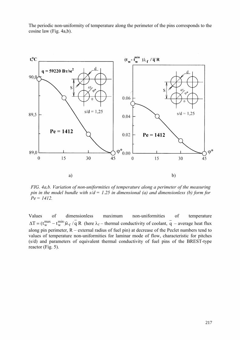
The periodic non-uniformity of temperature along the perimeter of the pins corresponds to the cosine law (Fig. 4a,b).

a) b)

FIG. 4a,b. Variation of non-uniformities of temperature along a perimeter of the measuring pin in the model bundle with s/d = 1.25 in dimensional (а) and dimensionless (b) form for Pe = 1412.

Values of dimensionless maximum non-uniformities of temperature Rq/)tt(T f

minw

maxw λ−=Δ (here λf – thermal conductivity of coolant, q – average heat flux

along pin perimeter, R – external radius of fuel pin) at decrease of the Peclet numbers tend to values of temperature non-uniformities for laminar mode of flow, characteristic for pitches (s/d) and parameters of equivalent thermal conductivity of fuel pins of the BREST-type reactor (Fig. 5).

217

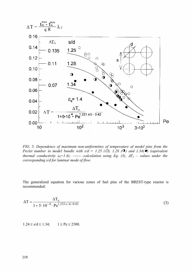
FIG. 5. Dependence of maximum non-uniformities of temperature of model pins from the Peclet number in model bundle with s/d = 1.25 ( ), 1.28 ( ) and 1.34( ) (equivalent thermal conductivity ε4=1.4); ⎯⎯ -calculation using Eq. (3), ΔTл – values under the corresponding s/d for laminar mode of flow.

The generalized equation for various zones of fuel pins of the BREST-type reactor is recommended:

42.0d/s233.14л

Pe1051TT −− ⋅⋅+

Δ=Δ (3)

1.24 ≤ s/d ≤ 1.34; 1 ≤ Pe ≤ 2300.

218

Values of TΔ are obtained from the calculated data.

Heat transfer of fuel pins with two spacer grids (εр = 20%) is a little bit higher (approximately 15%) then heat transfer for fuel pin with one spacer grid [6]. For an investigated range of Peclet numbers universal criteria dependence (2) is recommended in which factor a for considered case is 0.0115.

In the field of small Peclet numbers, there is a passage to the limit of Nusselt numbers to values of laminar mode of coolant flow in the subassembly without spacer grids. According to Eq. (2) growth of heat transfer in accordance with transition from smooth pins to pins with one and then with two spacer grids is the result of, as already it was marked, the turbulent component in the Nusselt number, that is reflected by values of the factor a for one (a = 0.009) or two (a = 0.0115) spacer grids on comparison with smooth pins (a = 0.007). For small flow rates of coolant the effect from availability of spacer grids (one or several) in the relation of heat transfer is absent practically.

3.2. Irregular model bundle with one spacer grid

Main regularities for temperature fields of the measuring model pin located on the boundary of zones with various diameters and powers of model pins (Fig. 2b) [7, 8] let us consider for an experiment with small flow rate of coolant (Re = 3030) and large ratio of power of zones (N15 / N10 = 2.0), when the characteristic regularities are exhibited most precisely (here N15 and N10 – power of model pins in zones of model assembly with an amount of model pins 15 and 10 accordingly).

3.2.1. Periodic non-uniformity of temperature

At small distances from a beginning of energy release (up to the spacer grid) coolant heating in cells round the measuring model pin differ weakly even for large distinction powers of model pins (N15 / N10 = 2.0) in zones with s/d1 = 1.25 and s/d2 = 1.46. It creates conditions for appearance of periodic non-uniformities of temperature along the perimeter of the model pin. The dimensionless non-uniformities of temperatures reduced to a cell 0–45° are changed under the cosine law (similarly to Fig. 4b) and do not reveal any certain dependence on value of jump of energy release. The dimensional non-uniformities depend on jump of energy release at zones as the modification of relative energy release N15 / N10 assumes modification of value of specific heat flux at the surface of adjacent model pins.

3.2.2. General non-uniformity of temperature

In an item of the thermocouple №3 (and further along zone of energy release) the general non-uniformity of temperature along the perimeter of model pin stipulated by a difference of heating of coolant at “boundary” cells for distinguished powers of pins in zones is exhibited.

The general non-uniformity of temperature along the perimeter of the measuring model pin is determined by temperature difference in points of the perimeter ϕ = 0° and 180° (maximum – at ϕ = 0°, minimum –at ϕ = 180°) (Fig. 6a).

219

FIG. 6. Comparison of temperature fields around the perimeter of the measuring model pin with one and two spacer grids (a); variation of surface temperature of the measuring model pin around the perimeter in the various cuts along length of the zone of energy release (thermocouple №8 – 12) for⎯Pe = 63 and N15 / N10 = 1,0 (b), R – external radius of the model pin,⎯q – average heat flux around the perimeter of the model pin.

220

And on the contrary, if the power in the zone with c s/d2 = 1.46 considerably exceeds power in the zone with s/d1 = 1.25 (N10 / N15 = 2 – “reverse” jump of energy release to considered jump), the general non-uniformity of temperature is determined by maximum at ϕ = 180° and minimum at ϕ = 0°.

In some operational modes of model assembly (especially for transitional current of coolant from laminar to turbulent) effect of “displacement” of temperature maximum along the perimeter of the model pin in different cross-sections along length of the zone of energy release (Fig. 6b)*) occurs: the thermocouple №8 fixes a profile with maximum at ϕ = 0°, thermocouple №9 –at ϕ = 60°; №10 – at ϕ = 120° etc. (increase of number of the thermocouple corresponds to increase of distance from a beginning of energy release).

Maximum general non-uniformities of the measuring model pin are illustrated in Fig. 7 (the dimensionless form) as the function of jump of energy release at fixed flow rate (Pe, Re numbers) of coolant (the field of temperature is shown in Fig. 6a). As it is visible, these are linear dependences (more strict – at greater flow rates of coolant), demonstrating increase of non-uniformities with increase of the relative jump of power N15 / N10 and with decrease of Pe (Re) number.

At “reverse” jumps of power when the redistribution of position of a maximum and minimum of temperature at the points ϕ = 0° and 180° happens, the non-uniformity of temperature is conditionally postponed downwards from zero on the ordinate axis and the sign “minus” is given to it.

The modification of relative energy release in adjacent zones of model pins of model subassembly is investigated in a more broad interval than it can be in the core of the BREST-type reactor; the experimental data for nominal Pe numbers of the reactor (~2000) are reproduced by a reliable extrapolation; the final recommendations for the reactor base on use of the greatest values of general non-uniformities of temperature from the indications of thermocouples located at the outlet of the zone of energy release of the model subassembly. In the core of the BREST-type reactor the greatest non-uniformities of temperature also will take place at the outlet of zone of energy release where distinction of heating in adjacent cells is maximum.

*) Pe and Re numbers used in Fig. 6b, and further (Figs 7 and 8) are calculated from average velocity w in the cross-section of assembly and from hydraulic diameter of a regular cell in the zone with s/d1 = 1.25. The velocity in the cell s/d1 = 1.25 is practically equal to the velocity to velocity w .

221

f

minw

maxw

1 RqttT λ

−=Δ

FIG. 7. Dependence of general non-uniformities of temperature around the Perimeter of the measuring model pin on jumps of energy release N15 / N10 and Peclet numbers (experiment with one spacer grid).

222

3.3. Irregular model bundle with two-spacer grid

“Interaction” of adjacent spacer grids can reduce temperature non-uniformities in the fuel subassembly (especially in irregular zones), increase heat transfer (it was noted above) and as a whole to have a positive effect on temperature modes of fuel pins of the BREST-type reactor.

Characteristics of a temperature field around the perimeter of the model pin (Fig. 6а) is (as well as in the experiments with one spacer grid) maximum of surface temperature of the model pin in the “narrow” zone of model assembly (s/d = 1.25, narrow gap between model pins – ϕ = 0°) and minimum in the “wide” zone of model assembly (s/d = 1.34, gap between model pins at ϕ = 180°)*). It determines general non-uniformity of temperature along the perimeter of the model pin stipulated by overheating of the coolant in the zone with s/d = 1.25 and underheating in the zone with s/d = 1.34.

In Fig. 6a the average temperature fields in the second half of model subassembly from the indications of several thermocouples are illustrated when the distributions are characterized by smaller value of temperature non-uniformity on comparison with non-uniformity at the outlet of the zone of energy release. The experiments have shown that a ratio between non-uniformities of temperature of compared variants (subassembly with one and with two spacer grids) is the same for various cross-sections of the bundle (including for the cross-section at the outlet of the zone of energy release representing the greatest practical interest). This ratio remains the same for illustrated in Fig. 6a average values of non-uniformities of temperature from indications of several thermocouples.

Determined from the experiments with one spacer grid the linear dependence of non-uniformity of temperature on relative power N15 / N10 in a broad band of a modification N15 / N10 (0.5 ÷ 2.0) in general is confirmed by experiments with two spacer grids, though the range of modification of relative powers in these experiments was essentially less (0.82 ≤ N15 / N10 ≤ 1.20). It allows to conduct recalculation of obtained regularities for relative power N15 / N10 = 1.0 to other values N15 / N10.

The dependence of dimensionless non-uniformity of temperature on Peclet number for using both one spacer grid (ΔT1) and two spacer grids (ΔT2) is shown in Fig. 8. It is visible, that the non-uniformities are not so hardly changed in the field of large Peclet numbers (Pe > 700), but sharply increase with decrease of Peclet number in the area Pe < 300 ÷ 400 (rate of increase ΔT1 and ΔT2 is about identical). The non-uniformity ΔT2 is ∼0.52ΔT1 for Pe ≅ 100 and ∼0.42ΔT1 for Pe ≅ 1300. Dependence ΔT2 / ΔT1 on Pe is approximately linear. It is possible to accept approximately ΔT2 ≅ 0.47ΔT1 in investigated range of modification of Peclet numbers (100 ≤ Pe ≤ 1300).

For analysis of the case under consideration for the core of the BREST-type reactor it is necessary to use the values of ΔT1 from the nomogram represented in Fig. 7.

The problems of further thermohydraulic research are to study various kind of thermohydraulic heterogeneities in the subassemblies caused by availability of fuel pins with different diameters and energy release, supporting tubes and displacers, contact of the core

*) The intermediate cell between zones s/d1 = 1.25 and s/d2 = 1.46 is considered as conditionally regular cell if its relative pitch s/d = 1.34 is calculated using average diameter⎯d = (d1+d2)/2.

223

with the side reflector, temperature fields of the deformed lattice of fuel pins, factors of overheating, influence of contact thermal resistance to temperature modes of fuel pins, etc.

FIG. 8. Dependence of dimensionless temperature non-uniformity on Peclet number for using one (ΔT1) and two (ΔT2) spacer grids.

REFERENCES

[1] ORLOV, V.V., New Stage of Nuclear Power and Fast Reactors Cooled by Lead, Information Newsletter №3 (10) Nuclear society USSR (1991) p. 6 (in Russian).

[2] ADAMOV, E.O., ORLOV, V.V., Development of nuclear power on the basis of the new concepts of nuclear reactors and fuel cycle, Proc. Conf. on Heavy Liquid Metal Coolants in Nuclear Technology (HMLC’98), 1998, Obninsk, Russian Federation, SSC RF, CRS4, TECH-REP-00/50 (1999) p. 15 (in Russian).

[3] KUZINA, J.A., SMIRNOV, V.P., ZHUKOV, A.V., SOROKIN, A.P., Research of temperature fields and heat transfer on the model fuel assembly for the lead cooled fast reactor, Proc. Scientific Session MIFI-2000, MIFI, Vol. 8, Moscow, Russian Federation (2000) pp. 108–110 (in Russian).

224

[4] KUZINA, J.A., Thermohydraulic problems of reactors with inherent safety features, Proc. XIII School-Seminar of Young Scientists and Specialists under the leadership of the Academician, Professor A.I. Leontiev “Physical Principles of Experimental and Mathematical Simulation of Heat and Mass Transfer and Gas Dynamics in Power Plants, Saint Petersburg, Vol. 2 (2001) pp. 469–472 (in Russian).

[5] ZHUKOV, A.V., KUZINA, J.A., SOROKIN, A.P., et al., Experimental Research of Heat Transfer in the Core of Lead Cooled BREST-OD-300 Reactor Using Models, Thermal Engineering, №3 (2002) pp. 2–10 (in Russian).

[6] KUZINA, J.A., SILA-NOVITSKY, A.G., Model Experiments and Calculations (TIGR-BRS code) for Study of Temperature and Velocity Fields in the Cores of the Reactors with Heavy Coolant, Thermal Engineering, №11 (2002) (in Russian).

[7] KUZINA, J.A., ZHUKOV, A.V., OREHOV, M.V., Research of Temperature Fields for Fuel Rods Located on the Interface of Subzones with Different Diameters and Energy Release of Fuel Rods (for Reactors such as BREST), Abstracts VII Int. Conf. NPP Safety and Personnel Training, Obninsk, Russian Federation (2001) pp. 24–25 (in Russian).

[8] KUZINA, J.A., ZHUKOV, A.V., OREHOV, M.V., et al., Temperature Fields of Fuel Pins in The Core of the BREST-OD-300 Reactor (Experiments Using Model Assemblies), Proc. Scientific Session MIFI-2002, MIFI, Vol. 8, Moscow, Russian Federation (2002) pp. 44–45 (in Russian).

225

PRE-TEST ANALYSIS OF THE MEGAPIE INTEGRAL TEST WITH RELAP5

W.H. LEUNG, B. SIGG Paul Scherrer Institute (PSI), Villigen, Switzerland

Abstract

MEGAPIE Integral Test is an experimental program for system integration and functional test of the newly designed liquid Lead-Bismuth Eutectic (LBE) target system to be performed before target irradiation. This LBE target is designed for spallation neutron generation by bombarding it with a high-energy proton beam and it also serves as experimental demonstration of the technical feasibility of using an LBE target in accelerator driven systems. A RELAP5 model is built to the specifications of the Integral Test, which by and large simulates the original configuration in the irradiation test. The heat-removing capacity is studied by using a detailed model of the target heat exchanger (THX) and by comparison with available experimental results. For the modeling of the friction loss, the best-known correlation available is being used. The study of the general thermal-hydraulic behavior of the target aims at ascertaining the effects of buoyancy on the flow characteristics. Scaled experiments are planned for the heated and transient tests. While the nominal power of the target is 581 kW, the electric heater for the Integral Test can provide only up to 200 kW because it depends on available heating technologies. The paper shows that, if operation conditions are scaled properly, buoyancy effects can correctly be accounted for and that the distortion of the dynamic behavior can be compensated if thermal-hydraulic effects are modeled accurately by RELAP5.

1. INTRODUCTION

The MEGAPIE Initiative [1] is a joint European research program for designing, manufacturing, operating, and decommissioning of a 1 MW spallation neutron target, i.e. for demonstrating its technical feasibility. The technical know-how building up in the process can help to assess the feasibility and to assist the design of a transmutation reactor for incinerating long-lived nuclear waste. Thus the MEGAPIE experiment is an important milestone towards realizing the Accelerator Driven Systems (ADS). A large array of research programs have been launched in the areas of nuclear assessments, thermal-hydraulics, structure mechanics, liquid metal technology, materials science, and radiation damage. The one especially aimed at the design, construction, and testing the target system is named MEGAPIE Test, in which extensive test programs of the components towards realizing the complete system are planned. The final test of the target system will be the irradiation test in the Spallation Neutron Source (SINQ) in Paul Scherrer Institute (PSI). But before the irradiation test can be conducted, all the ancillary systems and the target must be assembled together, integrated, and tested together in the Integral Test. During the Integral Test, the proton beam will be simulated by an electric heater. All the functions of the target and the ancillary systems will be tested together with the control system. The core of the Integral Test is to characterize the thermal-hydraulic system and its heat removal capacity. After all, the proton beam deposits 581 kW of thermal power into the target, which must be reliably removed.

One of the design constraints is that the new MEGAPIE target must fit into the existing target cavity of the SINQ facility. The schematic of the SINQ facility is presented in Fig. 1. The target is oriented vertically and the proton beam is inserted through the beam window at the bottom of the target. The target material LBE also serves as primary coolant. The target system has gone through an elaborated conceptual design study and many different options have been considered. The final design of the target presented in Fig. 2 shows that the target can be divided into two parts: the upper target and the lower target.

227

FIG

. 1. T

he s

ide

view

of t

he S

INQ

faci

lity.

The

targ

et is

inse

rted

from

the

top

into

th

e ca

vity

, and

the

activ

e re

gion

is a

t the

bot

tom

of t

he ta

rget

(ce

nter

poi

nt o

f the

fig

ure)

.

FIG

. 2.

The

MEG

APIE

liq

uid

met

al t

arge

t w

ith s

ome

deta

ils d

imen

sion

s of

the

uppe

r ta

rget

(i.e

., TH

X) a

nd th

e lo

wer

targ

et (i

.e. d

ownc

omer

, ris

er, a

nd c

entr

al ro

d.

228

The upper target consists of two submerged Electro-Magnetic Pumps (EMPs) and a 12-pin Target Heat eXchanger (THX). The two pumps are the main EMP that supplies the main flow for the target heat removal, and the bypass EMP that provides the LBE jet for beam window cooling. The lower target consists of the downcomer, beam window, riser, and central rod. The downcomer guides the colder fluid from the THX exit to the beam window. After the flow passing the beam window, it turns upward into the riser. The proton beam penetrates the liquid LBE to a depth of 250 mm. The region heated by the proton beam is called active zone. The downcomer and the riser are separated by a non-insulated, thin-wall guide tube. A substantial amount of heat is transferred from the riser to the downcomer, heating up the LBE in the downcomer before it reaches the beam window.

The target material LBE is also the coolant that transports the heat from the active zone to the THX. The secondary side of the THX is connected to the Intermediate Cooling Loop (ICL), which is filled with the organic coolant Diphyl THT (DTHT). DTHT is chosen for its favorable properties at the operating temperatures, i.e. its low vapor pressure (boiling point at 360°C) and stability in an irradiated environment. The ICL is a closed loop consisting of the Intermediate Heat eXchanger (IHX) that transfers the heat from the ICL to the Secondary Water Loop (SWL), which is sandwiched between the ICL and the building cooling plant. The Secondary Heat eXchanger (SHX) finally transfers the heat from the SWR to the building loop. This design has been chosen for protecting the cooling plant from DTHT contamination in case of a leak in the IHX. For safety reasons, the operating pressure in the ICL is higher than in the target and the SWR. The three loops together form the Heat Removal System (HRS) of the MEGAPIE target. A Schematic of the complete system is presented in Fig. 3.

FIG. 3. The schematic of the heat removal system.

The HRS is one of the ancillary systems and its thermal-hydraulic properties are one of the key interests of the planned tests of the MEGAPIE target. There are 3 more sub-systems dealing with the different needs before, during and after target irradiation which are the:

229

(a) Cover Gas System (CGS): to deal with the radioactive gas and volatile spallation products in the cover gas during the irradiation experiments,

(b) Fill and Drain System (F&D): to drain inactive LBE from the target for transportation and filling up the target after its installation in SINQ. It is required because the target must be tested for its functionality and operability outside SINQ,

(c) Insulation Gas System: to insulate between the hot target liquid metal containers and target enclosure.

Each of these ancillary systems is specially designed for a specific function. During most of the time they are operated independently and when the target is not being irradiated. The system that matters most during normal operation of the target is the HRS, because the heat deposited by the proton beam must be removed from the target.

2. THE MEGAPIE INTEGRAL TEST

Target and ancillary systems are each of them first of their kind and have not even been tested as separate systems. A control system is being developed independently for integrated operation of the combined system. There are needs for testing the component functions in the system and the combined functions of the target systems. Furthermore, it is necessary to prove to the safety authority as well as to the PSI-internal responsible body that the target and the ancillary systems are reliably operable as single systems and in combination. In this light, the Integral Tests are being planned. Very extensive tests will be conducted to investigate the main functions of the target system. It is however beyond the scope of this paper to discuss the details of the test plan, which can be found in the report of MEGAPIE Test [2]. The focus here is on the thermal-hydraulic experiments that will be conducted in the in the Integral Test. A special test facility, called the MEGAPIE Integral Test Stand (MITS), has been built to house the target system. Figure 4 is a 3-D sketch of the target system configuration on MITS.

FIG. 4 The target system on the MITS.

230

Note that this configuration is an exact replica of the system layout for SINQ, except for the HRS. The HRS has the SWL on the main floor that is below the Target Head and the ICL, but in SINQ, the SWL will be situated above the ICL. Furthermore, the pipes connecting the SWL to the IHX are much shorter in MITS than in SINQ, but pipe volumes are equal in both configurations. An important part of the Integral Test is the thermal-hydraulic experiments on the HRS. Since the electric heater cannot achieve the high power density of the proton beam, the heating power must either be reduced or the lower target has to be enlarged to accommodate sufficient heaters for making up the total power of the beam. Arguments put forth for determining the heater power are summarized in Table 1.

Since the heater is attached to the bottom of the Lower liquid-Metal Container (LMC), it is called LMC Heater.

It is clear that the mid-range is some kind of worse choice, because the time scale distortion is compounded by both volume increase and velocity reduction. If full power cannot be realized, the second best is the 150~250 kW range. Note that a heater power below 150 kW is not considered, because it is too low for any meaningful heated experiment. The lowest range has been selected for it entails the least distortion to the lower target geometry. A design of the heater is presented in Fig. 5. It is a 19-pin bindle that arranged hexagonally array with a pitch (between the pins) of 24 mm. The heater pins are measured 16 mm in diameter and 600 mm in total length with 100 mm non-heated length. The lower liquid metal container (LLMC) is modified. A new a double-flanged LLMC replaces the original one. A flanged connection is made so that the LMC Heater can be inserted from the bottom. A small semispherical calotte is fitted to the bottom when the heater is removed. In this way, the original geometry can be restored for the hydraulics test of the system. Figure 6 presents the lower target configuration with and without the LMC Heater during the Integral Test.

TABLE 1. THE OPTIONS OF LMC HEATER Heater power

(kW) Configuration/extra

LBE Vol. Scaling factors of mass flow rate/ temperature rise

Time distortion in transient events

> 500 External heater container/ + 23.4 L

0.95~1.0 / 0.90~1.0

Due to increased LBE volume

250~500 External heater container/

+ 14.7 L 0.75~0.95 / 0.57~0.90

Increase due to increasedvolume and reduced velocity of LBE

150~250 In main flow guide /

- 3.8 L 0.64~0.75 / 0.41~0.57

Increase due to reduced LBE velocity

231

FIG. 5. The iso and top views of the LMC heater.

FIG. 6. The configurations of the lower liquid metal container duringthe integral test.

3. MODELING THE TARGET SYSTEM IN MITS

The target system is a multi-loop, multi-fluid system, namely:

(i) The primary lead-bismuth eutectic (LBE) loop (target as well as coolant); (ii) The intermediate Diphyl THT (DTHT) cooling loop (ICL); and

(iii) The secondary water loop (SWL) sandwiched between the ICL and cooling plant of the experimental hall (see Fig. 3).

A model is developed for RELAP5/Mod 3.2 in the Integral Test configurations so that the actual system behavior can be studied. The nodalization of the MEGAPIE target HRS on the MITS is presented in Fig. 7. The SWL is installed below the ICL in the Integral Test, contrary to the SINQ. The pipes connected between SWL and ICL are also shorter on the Test-Stand, but the total volume of the system remains the same in order to preserve the hydraulic characteristics of the system.

RELAP5 is a system code developed for analyzing the Loss Of Coolant Accidents (LOCA) in a light water reactor (LWR) system [3]. The main working fluids are obviously water and steam. The thermal physical properties of water and steam are already available with the code, but those of the LBE and DTHT must be modeled and input to the code. The properties of LBE have been generated using the data of Lawrence Livermore Laboratory [4, 5]. Reference Diphyl-THT properties have been obtained from the manufacturer and generated using a model developed by Ansaldo [6].

Although there are 3 fluids in the system, they are separated in their own loops. Each one of them is a simple single-phase loop. Friction losses can be calculated by a simple model such as:

232

(1)

where ΔPfirc, Cf, L, D, Kloss, ρ, m and A are the frictional pressure drop, friction coefficient, channel length, hydraulics diameter, inlet loss, liquid density, reference mass flow rate, channel cross section area, respectively. The subscript n denotes the number of the channel. The friction coefficient, Cf, is well known and the same standard correlation can be applied to all fluids (including liquid metal). However, it is not the case for the loss coefficient, Kloss, which must be dealt with in a more elaborated way. Inside the target, there are inlets and outlets for which the loss coefficients cannot be taken from any standard designs. One good example is the entrance of the riser above the beam window, and another one is the bypass flow-channels. The details of how these entrance losses are modelled are reported in Ref. 7.

The RELAP5 code enables a pump model to be included by using its characteristic pump curve in the input deck. The pumping mechanism of an EMP is quite different from a centrifugal pump, but it is modeled in the same way as a mechanical pump. The Main EMP is modeled on the basis of the test results for the prototype [8]. As for the bypass EMP, only the design curve is available at this moment. The models of the centrifugal pumps in ICL and SWL are based on the curves supplied by the manufactures.

The other important component in the target is the THX. It is a 12-pin design arranged in 2 semicircles. All the pins are supposed to be identical. Single-pin tests have been conducted by Agostini [9]. The experimental heat transfer coefficients of LBE and DTHT are plotted in Fig. 8.

FIG. 7. Nodalization of the MEGAPIE target heat removal system in the MITS configuration.

FIG. 8. The experimental results the prototype EMP (for the target Main EMF).

nnlossffric A

mKD

CP ∑⎥⎥⎦

⎤

⎢⎢⎣

⎡⎟⎠⎞

⎜⎝⎛

⎟⎠⎞

⎜⎝⎛ +=Δ

2

21ρ

233

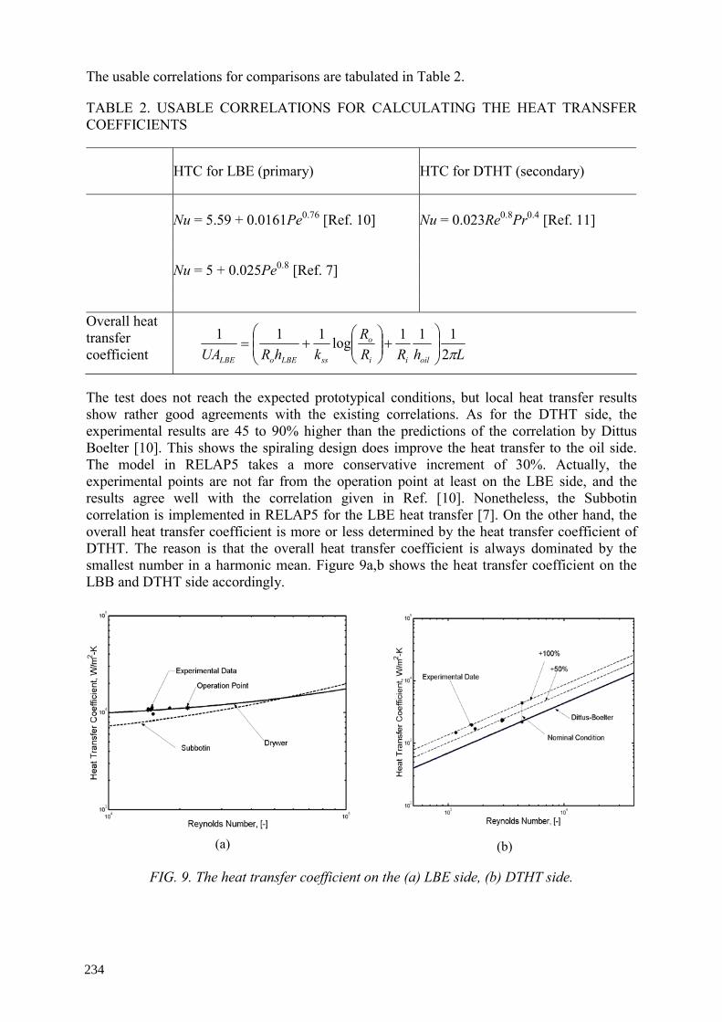
LhRRR

khRUA oilii

o

ssLBEoLBE π2111log111

⎟⎟⎠

⎞⎜⎜⎝

⎛+⎟⎟

⎠

⎞⎜⎜⎝

⎛+=

The usable correlations for comparisons are tabulated in Table 2.

TABLE 2. USABLE CORRELATIONS FOR CALCULATING THE HEAT TRANSFER COEFFICIENTS

HTC for LBE (primary) HTC for DTHT (secondary)

Nu = 5.59 + 0.0161Pe0.76 [Ref. 10] Nu = 0.023Re0.8Pr0.4 [Ref. 11] Nu = 5 + 0.025Pe0.8 [Ref. 7] Overall heat transfer coefficient

The test does not reach the expected prototypical conditions, but local heat transfer results show rather good agreements with the existing correlations. As for the DTHT side, the experimental results are 45 to 90% higher than the predictions of the correlation by Dittus Boelter [10]. This shows the spiraling design does improve the heat transfer to the oil side. The model in RELAP5 takes a more conservative increment of 30%. Actually, the experimental points are not far from the operation point at least on the LBE side, and the results agree well with the correlation given in Ref. [10]. Nonetheless, the Subbotin correlation is implemented in RELAP5 for the LBE heat transfer [7]. On the other hand, the overall heat transfer coefficient is more or less determined by the heat transfer coefficient of DTHT. The reason is that the overall heat transfer coefficient is always dominated by the smallest number in a harmonic mean. Figure 9a,b shows the heat transfer coefficient on the LBB and DTHT side accordingly.

(a) (b)

FIG. 9. The heat transfer coefficient on the (a) LBE side, (b) DTHT side.

234

3/2

⎟⎟⎠

⎞⎜⎜⎝

⎛=

ΔΔ

n

s

n

s

QQ

TT

4. SCALING RATIONALE AND RESULTING TEST CONDITION IN MITS

The proton beam heating is simulated by an electric heater attached to the bottom of the LMC. This electric heater cannot reach the power density of the proton beam, unless the lower target is expanded to a much larger tank. The question is whether the experiments conducted at a much lower heating power are relevant to nominal operation in the proton beam. It is difficult to answer this sort of question, because numerous parameters are distorted when heating and flow rates are changes.

Since the target is operated in a mix-convection mode (i.e., the buoyancy has a significant contribution to the driving head), it has been decided to scale the operating conditions in such a way that the relative contribution of the buoyancy head is preserved. The reasoning goes as the follows:

(i) The buoyancy head, ΔPgrv, is proportional to the temperature difference ΔT (Boussinesq approximation);

(ii) The temperature difference, ΔT, is directly proportional to the power input, Q, but inversely proportional to the mass flow rate m;

(iii) The flow resistance, ΔPfric which counteracts the buoyancy, is proportional to the square of the mass flow rate, m2;

(iv) All put them all together, the flow rate and the temperature can be scaled as:

and

respectively, (2)

where

the subscripts n and s are denoting the nominal and scaled conditions, respectively.

In order to determine the operating conditions of scaled-down experiments, the nominal conditions in SINQ must be specified first. Taking nominal operating conditions for 581 kW of proton beam heating from the study of Leung [12], the scale- down conditions for 200 kW in MITS can be computed. Note that the total power of the LMC Heater has yet to be fixed, but 200 kW is not too far from reality. This gives a power ratio of 0.34. Using the above relationships of flow rate and power, one can obtain the scaled-conditions for the 200 kW-operation. The scaling results of scaling are summarized in Table 3a and 3b.

3/1

⎟⎟⎠

⎞⎜⎜⎝

⎛=

n

s

n

s

QQ

mm

235

TABLE 3a. NOMINAL AND SCALED PUMP HEADS, PUMP POWERS AND FLOW RATES OF EACH LOOP IN THE HRS

Heating power, kW SINQ 581

Integral test 200

Main 40.0 28.03 LBE Target Bypass 2.5 1.75

ICL-DTHT 8.0 5.61 Mass flow rate, kg/s

SWL-H2O 8.0 5.61 Main 22.8 16.5 LBE Target, A Bypass 17.8 12.7

ICL-DTHT, rpm 2749. 2196. Pump current/speed

SWL-H2O, rpm 2390. 2047. ΔPpump .116 .0623 ΔPgrv .0343 .0166 Main, LBE ΔPgrv/ΔPfric .228 .210

Bypass, LBE, ΔPpump 0.175 0.089 ICL-DTHT, ΔPpump 5.21 2.83

Pressure head, bar

SWL-H2O, ΔPpump 2.47 0.735

TABLE 3b. NOMINAL AND SCALED FLOW RATES, AND INLET AND OUTLET TEMPERATURES OF THE HEXS IN HRS

Heating power, kW SINQ 581

Integral test 200

Flow Rate, kg/s 40. 28.03 Tin, °C 327.2 272.6

Hot side, LBE

Tout, °C 230.0 230.0 Flow Rate, kg/s 7.90 5.61 Tin, °C 137.6 199.2

Target heat exchanger (THX) Cold side,

DTHT Tout, °C 174.4 215.2 Flow rate, kg/s 4.62 3.24 Tin, °C 175.2 215.2

Hot side, DTHT

Tout, °C 109.4 186.1 Flow rate, kg/s 7.96 5.58 Tin, °C 49.5 157.8

Intermediate heat exchanger (IHX) Cold side,

H2O Tout, °C 67.4 165.6 Flow rate, kg/s 6.62 4.64 Tin, °C 67.9 153.7

Hot side, H2O

Tout, °C 46.3 105.5 Flow rate, kg/s 8.00 5.61 Tin, °C 30.0 30.0

Secondary heat exchanger (SHX) Cold side,

H2O Tout, °C 47.9 39.13

236

FFdt

dErrAdtErrAErrACV DIP +++= ∫

One problem is that the operating temperature of the water loop becomes higher than the boiling point at the design pressure. To avoid boiling, the SWL must be pressurized to roughly 8~10 bars. Based on these results, the scaling achieved the primary objective; the buoyancy contribution is kept at around 20% of the main flow. A small difference may be due to the heat transfer through the HEX is not correctly modeled.

5. THERMAL HYDRAULIC TRANSIENT: PROTECTED BEAM TRIP

One of the important transients in MEGAPIE target operation is the proton beam trip, because the proton beam suffers hundreds of trips in a week’s operation and roughly 1×104 in the target life-time (roughly a year operation). Since the high power source is taken out abruptly, the high capacity HRS may chill the LBE down too much during the transition. More importantly, the target must be protected from thermal shock, especially for the beam window, to avoid excess thermal stress in the structure material. One of the options is to regulate the LBE temperature at some point at a constant temperature in all conditions. A basic PID (Proportional, Integral, Derivative) control algorithm has been implemented in the RELAP5. This control sequence can be expressed as:

(3)

where CV denotes the control value which is, in this case, the fraction opening of the 3-way valve (3WV) in either of the ICL and of the SWL, Err is the difference between the control variable and the reference level, FF denotes the feed-forward signal, and AP, AI, and AD are the multiplication factors of the proportional, integral and derivative parts of the control, respectively. In this study, the control variable is the LBE temperature at the exit of THX, and the reference temperature is 230°C (i.e. Err = TLBE,out – 230°C). The FF is the time derivative of the LBE temperature at the inlet of the THX (i.e. FF = CFF dTLBE,in /dt). In essence, the inlet and outlet LBE temperatures of the THX, and their derivatives are fed to an integral controller to actuate the 3-way valve in the ICL to bypass the IHX in case of a beam trip. Since the LBE is protected from large temperature fluctuation, this thermal transient is called “protected beam trip”. Another important aspect of this study is to examine whether the control process would be modified in the scaled experiments.

The initial conditions and the input files are obtained from the steady-state calculations. In other words, the results presented in Table 3 are the initial conditions for these transient calculations. A normal beam trip transient is defined as the follows:

─ Beam power falls instantly to zero; ─ Beam is shut down for 10 s; ─ Proton beam ramps up to full power in 20 s time.

These transient times are given for the actual proton beam transient in SINQ. For the scaled case of 200 kW, those times are prolonged because of the reduced flow rate. Then, the beam trip transient times become 14.3 s shut down and 28.5 s power ramp. It is argued that the control function should be scaled in the similar way, but it is not clear at this point how this can be done. The CV is a function of the Err and the gain factors (i.e. AP, AI, AD and AFF). Furthermore, it is a function of sampling time because control function is going to be implemented by a digital system (i.e. discretized Err, and its derivative and integrate). In RELAP5, the sampling time is merely the time step, which is determined by the program

237

itself. All the gain factors are set according to sampling time, and cannot be changed independently. Besides, the studying the control system is beyond the scope of this paper.

In order to simulate the beam trip in the Integral Test, the LMC Heater must be installed in the target. The heater structure absorbs/releases heat during a thermal transient. The thermal inertia of the heater thus affects the temperature transient in the liquid. In this computation experiment, the following two models of heater are used:

(A) The heater structure has no thermal inertia and the heater channels are not modeled (i.e. the original lower target geometry is used);

(B) The heater structure is modeled as a bundle of solid stainless steel rods and the heater channels are also modeled.

The results of case A are compared with nominal beam trip in SINQ. The temperature transients in the target and IHX, and the 3WV regulating history during a beam trip are presented in Figs 10 - 12. The (a)s represent the results of the nominal case and the (b)s represent the results of the scaled case. The observations are summarized in the following paragraphs.

Figure 10 presents the LBE temperature transients during a beam trip for both nominal and scaled cases. One must remember that the time in the scaled case is stretched by a factor of 1.43. Within the period of beam trip, the temperature transient at the top of the active zone (TAZ) and at the entrance of THX (TLBE,in) are similar and the in proportion between the nominal and scaled cases. Taking the recovery time as the time to reach 98% of the original temperature, it takes a little longer for TLBE,in to recover in the scaled case. There are some observable differences in the TAZ and TLBE,in curves between two cases beyond the period of beam trip. These are possibly due to the feedback from the cooling loops. It becomes more obvious in the temperature transient at the exit of THX (TLBE,out). The TLBE,out curve of the scaled case has double peaks that is not found in the nominal curve.

(a) (b) FIG. 10 a,b. The temperature transient in the target during a beam trip transient (a) nominal case in SINQ, and (b) scaled case in MITS.

238

(a) (b) FIG. 11a,b. The transient regulation curves of the 3WV in a beam trip transient (a) nominal case in SINQ and (b) scaled case in MITS.

(a) (b)

Fig. 12 a,b. The temperature transients at the IHX (in both primary and secondary sides (a) nominal case in SINQ, and (b) scaled case in MITS.

239

To examine differences further, it is necessary to investigate what happens downstream of the THX. The transient curves of the 3-Way Valves (3WVs) are presented in Fig. 11. The 3WV-ICL curved in 11(b) is very different from the corresponding curve in 11(a). The feedback from the SWL is quite different. This becomes much clearer in the temperature transients in IHX that are shown in Fig. 12. One of the possible reasons is that a much smaller HEX is used instead of the SHX in the scaled case. The reason of using a smaller HEX is that the oversized SHX does not allow a large temperature difference to be obtained between the hot and cold side. While the building cooling plant is working at a constant temperature of 30°C, it is impossible to operate the SWL at higher temperatures than required by the scaled condition (see Table 3b). This small HEX does modify the transient conditions.

For case (B), the heater is modeled as solid steel. This probably exaggerates the effect quite a bit, but in this way the differences become more prominent. The scaled beam trip case is re-run and the results are presented along with the previous case in Figs 13 and 14, respectively. It clearly shows that the temperature transient at the top of the active zone is smoothed out quite a lot by the thermal inertia of the heater (see Fig. 13). This effect propagates upward to the inlet of the THX. A more diffused change of TLBE,in is felt by the control that regulates the ICL-3WV at a slower pace. This effect propagates downstream from the THX to the cooling loops. The temperature transients in the IHX are all shifted accordingly. The temperature transient in the IHX dose show the shifts due to a more diffused transient of TLBE,in. Of course the shift of the temperature transient in the ICL feeds back to the target through the THX and modifies TLBE,out.

FIG. 13. The target temperature transients during a scaled beam trip; the solid lines represent the heater without thermal inertia and the dashed line the heater modeled as steel rod bundle.

FIG. 14. The temperature transients in the IHX during a scaled beam trip; the solid lines represent the heater without thermal inertia and the dashed line the heater modeled as steel rod bundle.

Obviously, the thermal inertia of the heater and the changed size of the SHX modify the transient in a beam trip. The effect of the two components on the system behavior can however be visualized by comparing the numerical results of the different transients.

240

6. CONCLUSIONS

A general overview of the MEGAPIE Integral Test has been discussed. The original target and the ancillary systems will be tested as an integral system on the facility called MITS. Of major importance are the thermal-hydraulic experiments of target and HRS. A pre-test analysis conducted here shows that the scaling considerations provide a good basis for systematic investigations of the dynamic system behavior. The power of an LMC heater for simulating the proton beam heating is chosen to be in the range of 150~200 kW. For that range of the heater brings the least thermal-hydraulic distortion to the target. It is shown that inserting LMC heater to the riser brings negligible change to the hydraulic resistance of the target loop. The LMC heater slightly distorts the transient due to its thermal inertia, but by comparing numerical results obtained with RELAP5 with and without inertia this effect can be visualized. The thermal-hydraulic experiments will help to verify the used system models and to optimize the control function and control element behavior.

Currently, the thermal-hydraulic characteristics of the Integral Test studied with RELAP5 at the conditions of 200 kW. However, the actual heater power may be different from this work. If it is so, all the assessments will be redone for the power level of the actual LMC Heater.

REFERENCES

[1] BAUER, G.S., SALVATORES, M., HEUSENER, G., MEGAPIE, a 1 MW Pilot Experiment for a Liquid Metal Spallation Target, Proc. IWSMT-4 (J. Nucl. Mat.) and Proc. ICANS XV, JAERI-KEK Report (2001).

[2] LEUNG, W.H., SIGG, B., GROESCHEL, F., Report On Operational Procedures For Integral Test Of The MEGAPIE Target System, EU Report of Contract Nr. FIKW-CT-2001-00159 MEGAPIE Test, D19 (2003).

[3] RAMSOM, V.H., The RELAP5 Two-Fluid Model and Associated Numerical Method, Purdue University (1994).

[4] YOUNG, D.A., Soft Sphere Model for Liquid Metals, Lawrence LivermoreLaboratory University of California UCLR-52352.

[5] ANSALDO, Lead Bismuth Eutectic Physical Properties and Thermodynamic Tables, XADS 20 TRX 0003, Genoa, Italy (January 2002).

[6] ANSALDO, Mathematical Model and Thermophysical Properties Correlations forOrganic Heat Transfer fluids, ADS 1 TRIX 0244 rev.1, Genoa, Italy.

[7] PETRAZZINI, M., ALEMBERTI, A., Input and RELAP5 Model Description, Ansaldo Report MPIE 1 TRIX 200, Genoa, Italy (September 2002).

[8] DEMENTJEV, S., et al., EMPS for MEGAPIE Target − Testing of the Prototype, PSI Internal Report Nr: MPR-11-DS-34-005/0 (2003).

[9] AGOSTINI, P., Observations Resulting From MEGAPIE Cooling Pin Tests inBrasimone, ENEA Report: MP-T-R-001, ENEA, Brasimone, Italy (August 2002).

[10] FOUST, O.J., Sodium-Na-K Engineering Handbook, Vol. II, Gordon and Breach Inc., NY (1978).

[11] INCROPERA, F.P., DEWITT, D.P., Fundamentals of Heat and Mass Transfer, JohnWiley & Sons, 3rd edition, (1990) p. 496.

[12] LEUNG, W.H., On The MEGAPIE Target Thermal Hydraulics – A Relap5 Analysis, Submitted to, 12th International Conference on Nuclear Energy (ICONE-12),Arlington, Virginia, USA, 25–29 April 2004.

241

EXPERIMENTAL DETERMINATION OF THE LOCAL HEAT TRANSFER COEFFICIENT FOR MEGAPIE TARGET WINDOW USING INFRARED THERMOGRAPHY

J.A. PATORSKI, F. GRÖSCHEL Paul Scherrer Institute (PSI), Villigen, Switzerland

I. PLATNIEKS University of Latvia, Salaspils, Latvia

Abstract

In the scope of the Megawatt Pilot Experiment (MEGAPIE), i.e. a liquid metal target for a spallation neutron source, an experimental investigation (KILOPIE) of the target window cooling has to be performed. A reason to perform the KILOPIE experiment is that, in the area of the proton beam entry window, the values and distribution of the local convection heat transfer coefficient “α” for MEGAPIE conditions are unknown. The liquid metal, in this case lead-bismuth eutectic (LBE), is simultaneously used as target material and coolant. A hemispherical flow geometry made of T91 steel is used for the mockup of the proton beam entry window in an experimental set-up for a determination of the local convection heat transfer coefficient “α”. In KILOPIE two complementary methods are used for a determination of the local convection heat transfer coefficient “α”, the first one is the two dimensional Heat Emitting Temperature Sensitive Surface (2D-HETSS) method develop at PSI (Platnieks et al. [1]) and the second is an improved two-dimensional and dynamic infrared thermography (2DD-IRT) method, also developed at PSI (Patorski et al. [2]). In this paper only the methodology of improved 2DD-IRT will be presented. The experimental activities will be performed at the beginning of 2004 at Forschungszentrum Karlsruhe (FZK) using the THEADES loop of the KALLA laboratory and will be continued at Paul Scherrer Institute (PSI) using the new, consisting of two independent pumped circuits, PSI-LBE-Double-Loop. A specially tailored 0.053 mm thick Aluchrom YHf heating foil is used, which allows to apply a uniform and constant heat flux deposition on the outer surface of the hemispherical mockup-specimen of the target window. The optical non-contact IRT equipment measures the outer surface temperature of the mockup-specimen dish with a high space and time resolution, e.g. 1.25 mrad and 20 Hz. The 100 mm diameter of the mockup-specimen dish with approximately 5000 pixels, i.e. temperature measurement points, area of 1.6 mm2 is covering the area of interest, corresponding to the approx. 60 mm diameter of the proton beam footprint and results in temperature contour plots with good resolution. The dynamic capability of 2DD-IRT is essential for the investigation of the change of the local convection heat transfer coefficient “α” especially during transient load cases, i.e. during changes of the flow rate of the coolant. The accuracy of the temperature measurement is ±1%. The knowledge of constant heat flux and temperature differences between inner surface and coolant allow maks a two-dimensional dynamic determination and visualization of the local convection heat transfer coefficient “α”. In other words, the determination of the local convection heat transfer coefficient “α” is a result of ratio of the known local heat flux from the Aluchrom YHf heating foil to the difference between the local inner surface temperature and the bulk temperature of the LBE coolant.

1. INTRODUCTION

In scope of the long term R&D challenge to build an Accelerator Driven System (an industrial application of ADS is foreseen in year 2045), the creation of new concepts for spallation neutron sources with high neutron flux are the subject of world wide scientific investigations. A new concept of high power spallation source with liquid metal (LM) target is developed within the international MEGAPIE Project [3]. The experimental part of the MEGAPIE project will be performed in the spallation neutron source facility SINQ at Paul Scherrer Institute (PSI) in Switzerland. In the MEGAPIE target, the LM, in this case lead-bismuth eutectic (LBE) is simultaneously used as target material and coolant.

The general concept of the MEGAPIE target is shown in Fig. 1. Simplifying, a system of approx. 4 m long concentric cylindrical pipes and vessels, is fulfilling a LBE guiding and safety functions. The LBE flow-guiding part of the target consists of two steel pipes placed in the middle of the cross section of the target. The lower part of outer pipe is closed with a

243

hemispherical shell, forming a vertical, cylindrical liquid metal container (LMC) and causing a 180°-change of a downward LBE main flow “Q” into an upward flow in the inner riser pipe (RP). The 600 MeV proton beam comes through a lower enclosure of this system, the entry window. This window will be strongly heated; the heat deposition in the steel wall will produce a heat flux (q*) up to 140 W/cm2 [4]. (In one special case of wandering of the proton beam, the heat flux can be 200 W/cm2.)

� � � � � � � � � � � � � � �

� � � � � � � � � � � � � � � � �

� � � � � � � � � � � � � � � � � � � �

� � � � � � � � � � � � � � � � � � �

� � � � � � � � � � � � � � � � � � �

� � � � � ! � � " � � � � � � � � � �

# � � � � � � �

� ! � � � � � �

$ � � � � � � � � �

% � � � & � ! � � � �

� � � � � � � � � � ' � ( � � �

� � � � � � � � � � � �

� � � � � � � � � �

� � � � � � � � � � �

� � ) � � ) � � � � � �

��

( � �

� �

� � � � � # � � � � � � �

� � � � � � � � # � �

� � � � � � � � � � �

� � � � � � � � � � � �

� � � � � � � � �

� � � � � � � � �

� * � + , , � � $

FIG. 1. General concept of MEGAPIE liquid metal target for a spallation neutron source in SINQ facility at PSI.

This target window is cooled by an additional bypass pipe circuit so called the nozzle by-pass pipe (NBP). The open nozzle-end of the bypass tube forms an LBE jet flow “q” directly streaming onto the inner surface of the window.

Basic geometrical parameters of the assembled lower part of the target are displayed in Fig. 2 and represent the principal idea of pumped flow configuration: main flow “Q” and bypass jet flow “q” providing a transporting LBE to the spallation zone and a cooling for the hemispherical proton beam entrance window. The steel wall of the window will be cooled mostly by a LBE bypass nozzle jet flow “q” across the window area and additionally by main LBE flow “Q”. The main flow “Q” is responsible for recirculation and transporting the strongly heated LBE after spallation to the heat exchanger of the target, which is placed on the top of the whole target system.

244

������� ����*�������

��������

��� ���

���������

����

��

��

���

��

� �

� � � � � � � �

� � � � � � � � � � �

� � � � � �

� � � � � � �

$ � � � � � � � & � � � � � � � - � � � �

����������������������������� ���!���"��#�

. � � � � � � � � � � " � � � � � �

� � � � � � � � � � � � �

� � � � � � � � � � � ) � � � � � �

� � � � � � � � � � � � � � � � � � � �

������������/�0�11�

�!����������

�������2�2

# � � � � � � �

� � � � � � � � �

�����������������������

��� ���

� $ �

� �%

� &� �

� �%

��'��

��(�%

0 � 1 1 � � � � � � � � � � � � �

� � � � � � � � �

FIG. 2. Geometry of the lower part of the MEGAPIE target. Principal idea of the LBE-flow configuration.

2. GOALS OF THE EXPERIMENTAL INVESTIGATIONS

For a proper design and operation of the MEGAPIE target, the knowledge of the cooling characteristic of LBE flow for the specific geometrical flow configuration and for the real target window material, T91 (9Cr-1MoVNb) martensitic steel, is necessary. Therefore we have decided to perform a proper thermal hydraulic experiment

The main goal of the experiment is the determination of a local convection heat transfer coefficient α over the area of the proton beam entry window for different: ratios of characteristic LBE by-pass jet flow (q) and main flow (Q), geometrical flow configurations.

245

Other objectives are:

— Determination of optimal operating range for q and Q, similar to the work reported in Ref. [5].

— Validation of CFD calculations.

After performing the first phase experiments for the two different reference geometries (rectangular and round shape for the NBP and slanted RP) and small reference flow matrix; for Q (range 0.0–5.0 ) and q (range 0.0–1.0 ) the tuning and optimization of the reference configurations is planned. It could be done in a second phase, numerically as well as experimentally, by looking for the best configurations of easy changeable geometric parameters of the flow, labeled in Fig.2 as “A, B, C, D, E”. The angles “A”, “B” and dimensions “E” describe position, inclinations and shape of the NBP for bypass nozzle jet flow “q”. The angle “C” and the distance “D” are describing the slanted edge of the RP for the common “Q + q” upward flow.

With respect to the goals for planned experiments, we will simulate most conditions of MEGAPIE target: Materials (LBE and steel T91), the geometrical configuration (also with small variations), the bulk temperature of the LBE, local heat fluxes q* through the window, the main flow rate Q and bypass flow rate q. It should be especially mentioned here, that it is not necessary and above all not possible to simulate of full 1 MW power, resulting from the 600 MeV proton beam, that will be used for MEGAPIE target. Our pre–test estimations show that the heating power range that is necessary to achieve sufficient heat flux, is from 1 kW up to 10 kW. For this reason, we have named our investigation the KILOwatt PIlot Experiment (KILOPIE).

3. SET-UP OF KILOPIE IRT EXPERIMENT

As we know from our previous experimental activity, the use of Infrared Thermography (IRT) has been involved, with good results, within the Two-Dimensional and Dynamic Infrared Thermography (2DD-IRT) method, for the estimation of the flow characteristics in a convection boundary layer [2, 5]. The most interesting advantages of IRT are non-contact field temperature measurement techniques and high geometrical- (1.25 mrad) and time- (20 Hz) resolution. These advantageous features have been fully used for the visualizations produced by 2DD-IRT method.

With respect to our main goal, the expectation that IRT can open new insights into the phenomenology of the cooling process of the target window played a large role in the planning of the KILOPIE IRT-experiment. The entire set-up with all the instrumentation of the KILOPIE IRT -experiment is shown in Fig. 3.

The so-called “three flanged mock-up” of the lower part of the MGAPIE target (only inside dimensions) has been fabricated from stainless steel. The upper flange represents an interface to the THEADES loop of the KALLA laboratory at Forschungszentrum Karlsruhe (FZK) or an interface to the new double pumped circuits PSI-LBE loop at Paul Scherrer Institute (PSI). The second middle flange represents the interface to the so-called “vacuum chamber”, a device for realization of adiabatic boundary conditions for the IRT measured specimen. Controlling the surrounding ambient temperature reduces the radiation loss. And finally, a third small lower flange is fixing the intrinsic specimen, i.e. a simulation of the proton beam loaded area of the target window.

246

178

125122

40°

20 48

50

273.

526

4

TC TC

TC

TC

24/20

PC card thermocouplesTC measurement of LBEmain downwards flow "Q"bulk temperature

PC card thermo-couples TC mea-surement of LBEbypass jet flow q temperature

PC card thermo-couples TC tem-perature measu-rement of inner wall of the speci-men dish for IRTCalibration Pre-Test

Infrared Thermography (IRT)non contact temperatur field measuremnt of the heatingfoil with FLIR-AGEMAThermovision 900 IR Scanner

PC card measure-ment of DC powersupply(range 1 - 10 KW)

DC + 613

3 x Flangedmock-up of lower partof the target

Vacuumchamber & temperatur controledsurround-ing of IRTspecimen

Calcium FluorideIR window

Insertionsof RP and NBP

Specimendish &resistanceheating foil

AluminiumIR mirror

L > 1000 mm

FIG. 3. KILOPIE IRT experimental set-up and instrumentation.

The specimen (Fig.4) consists of a steel dish in the form of a 0.5 mm thin spherical cap manufactured from T91 (9Cr-1MoVNb) martensitic steel and a resistance heating foil glued on the outer surface of the dish with special procedure. The IRT scanner FLIR-AGEMA Thermovision 900 will measure the temperature field of the specimen from the distance of approx. 1 000 mm through the calcium fluoride crystal glass at the lowest part of the vacuum chamber. For safety reasons the IRT scanner is placed 90° out of the axis and take measurement from the reflected heat radiation in high quality polished aluminium IR mirror. It is necessary to save the expensive IRT scanner in the hypothetical accident case of the break of both the specimen dish and calcium fluoride IR window.

Also in the set-up schematic (Fig. 3) are shown the insertions, i.e. ending of the RP and NBP. As it was mentioned in Pt.2, these insertions are foreseen for easy change of geometrical flow parameters “A, B, C, D, E”. Additionally the 3-D view of an exemplary set of such insertions is shown in Fig. 5.

247

sphe

rical

Rin

n = 8

9.0

mm

75.50 mm1.0

mm

63.30 mm

0.5

mm

26.4

2 m

m

93 mm

88.8 mm

Specimen dish from T91 steel(9Cr-1MoVNb martensitic steel)in form of spherical capwith 0.5 mm thick wall

DC+

4 D

C P

ower

sup

plys

70 V

olt,

45 A

mpe

r

Aluc

hrom

YH

f hea

ting

foil,

δfo

il=0.

053

mm

To

tal h

eatin

g su

rface

of 6

6.4

cm2

Tota

l ele

ctric

resi

stan

ce o

f Rfo

il=5.

1 Ω

.

FIG. 4. KILOPIE IRT Specimen with resistance heating foil.

FIG. 5. Exemplary set of riser pipe (RP) and nozzle by-pass pipe (NBP) insertions .

248

4. RESISTANCE HEATING

A suitable heating mechanism for the window was chosen in view of optimizing the conditions for IRT- measurements and experimental goals. Thus the following measures and design choices were taken:

— To heat the target window by volumetric resistance heating inside the thin metallic foil glued to the outer surface of specimen. Such heating is well suited for use with IRT because heat reflection from the window surface is avoided. In the converse case of surface heating with an outside heat source the non-blackbody surface of the window reflects the external heat and disturbs the IRT measurements.

— To be able to realize the desirable and homogenous distributed heat flux value q* over the well known heating area.

— To screen the mockup with a surrounding anti-reflection vacuum chamber so as to avoid the effects of ambient heat sources at the sides (e.g. electric instruments/components or walking persons).

— To enhance the emissivity ε of the window surface (i.e. heating foil) and make it uniform. To this end the outer surface of the heating foil will be covered with special few micrometers thin alumina coating.

— To perform an exact calibration of the IRT equipment after each change of experimental configurations. The so-called emissivity chart technique will be used, which gives an individual value to the emissivity ε of each measurement pixel.

A temperature dependency of resistivity of candidate materials for the resistance heating foil as it is shown in Fig. 4. It is a big advantage to have the constant heat flux during the different cooling over whole area of observed temperature changes. The temperature distribution on the foil surface can differ in the range from LBE bulk temperature, e.g. 180°C, up to approx. 400°C, as in case of low efficiency cooling by the bypass jet stream. The comparison of possible condidate foils materials is shown in Fig. 6.

AlCr Steel

NiCr Steel

Lead

Iron

Tin

NickelPlatinum

Aluminium Gold

CooperSilver0.0E+00

3.0E-07

6.0E-07

9.0E-07

1.2E-06

1.5E-06

0 200 400 600 800 1000 1200Temperature [C°]

Res

istiv

ity [

Ohm

•m]

Aluchrom SteelNicrofer SteelLeadIronTinNickelPlatinumAluminiumGoldCooperSilver

FIG.6. Comparison of candidate materials for resistance heating foil.

249

Only one material has a constant value in this temperature range, namely the Aluchrom YHf ferritic steel (CrAl 20 5), with resistivity of 1.41E-6 Ω⋅m in the temperature range 200–400°C. Therefore we have used this material.

The suitable power supply has to cover the range from 332 W for the desired lowest heat flux of 5 W/cm2 up to 8300 W for the desired heat flux of 125 W/cm2. The gluing procedure to the steel dish has been done in two steps. The first one consists with covering the steel surface with a 0.050 mm thick layer of some kind of ceramic glue. The second step is the application of the steel foil with special epoxy glue. The thickness of this epoxy layer is 0.005 mm.

Most important for the determination of the local convection heat transfer coefficient “α” is precise determination of the heat flux. The meander tailoring of the heating foil with constant thickness 0.053 mm should guarantee the homogenous distribution of the total power generated in the foil over the whole heated specimen surface. The resistance of the foil is measured and known: foilR = 5.1Ω as well the area of the heated surface of the specimen

spherical cap laying under the foil: 239.66 cmAcap = . The desired heat fluxes, e.g. =*q 20, 40 and 60 W/cm2, allow for calculating the total power according the Eq. 4.1

captotal AqP ⋅= * (4.1)

The correspondings powers are,

=totalP 1327.8 W, 2655.6 W and 3983.4 W

According well known Ohm’s Law, Eq.4.2

foilfoiltotal R

URIP2

2 =⋅= (4.2)

where:

I DC current U DC voltage

we can calculate the desired current values that shoud be realised through the DC power supply units. The correspondings values are: 16.1 A, 82.3 V; 22.8 A, 116.4 V; 27.9A, and 142.5 V. The DC current values are simultanously measured and recorded with all other TC and IRT measurements.

5. INSTRUMENTATION OF KILOPIE IRT EXPERIMENTS

As shown in Fig. 3, the general instrumentation used in these experiments consists of two temperature measurement devices: the IRT equipment and the thermocouples TC scanning equipment.

The precise control that is needed to keep the pumping parameters of the loop at their prescribed values, to hold the heating constant and to maintain the security of the whole facility, will be assured by equipment belonging to FZK or PSI and which will not be described in this paper.

250

The IRT equipment of PSI (FLIR-AGEMA THV900 SWTE) is a non-contact measurement system, which allows 2D thermograms in the infrared short wave spectrum range (2–5.6 μm) to be registered. The IR- thermograms can be collected as single frames or as sequences. The time resolution for on-line recording by the IR-scanner and controller vary from 20 Hz for frames consisting of 128 lines at 204 pixels up to 3500 Hz for single lines of 204 pixels. The spatial resolution depends on the optic lens of the IR-scanner. In the SEH experiments a 10°-teleobjective lens with a spatial resolution of 1.25 mrad will be used. For a more detailed technical specification of FLIR-AGEMA THV900 SWTE, see User's Manual [6]

The data acquisition system for the TCs consists of a PC and a PC Kethley card. The data is recorded by special Testpoint® software created for both HETSS- and IRT-KILOPIE experiments [1].Very thin thermocouples (diameter 0.25 mm) of the “K” type, produced and calibrated at PSI by the group “Sensorik und Sonderverfahren” guaranteed response times shorter than 20 ms and reached the high accuracy of ± 0.2°C.

The data sets from the IRT and from the TC measurement must be recorded simultaneously. In order to achieve this synchronization, a special trigger unit was built and used to start each experiment.

6. IR CALIBRATION PRE-TESTS

The preparations described below are a part of the intense efforts that were made to measure the absolute temperature Tout.foil on the outer surface of the foil glued to the specimen dish. The difference to the absolute value Tbulk of the LBE bulk temperature is essential for the evaluation of the results.

The use of IR-thermography to derive absolute values of temperature requires the value of the emissivity ε, a radiative property of the surface, to be known. The emissive power E of the surface, which is the quantity directly measured in the IR-scanning, is less than the corresponding quantity Ebb of blackbody radiation at the same temperature and is given by the Stefan-Boltzmann law, Eq 6.1

4TE ⋅⋅= σε (6.1)

where:

ε - is emissivity; radiative property of the surface values in the range (0–1), σ - Stefan-Boltzman constant; (σ = 5.67 E-8 W/m² K4), T - absolute temperature in K.

For each measurement pixel, the emissivity can be expressed as a function of the spectral range λ , the temperature T, the direction of radiation φ (i.e. the angle between the view line and the normal to the radiating surface) and the roughness Ra :

( )aRTF ,,, φλε = (6.2)

Because the spectral λ-dependency of the IR scanner-detector is generally constant within the spectral range used (in our case λ = 2–5.6 μm), only the influence of the remaining three variables has to be considered for our experiments. These are: the cleanliness/roughness (Ra) of the surface, the position (i.e. the direction view angle φ) of the hemisphere relative to the

251

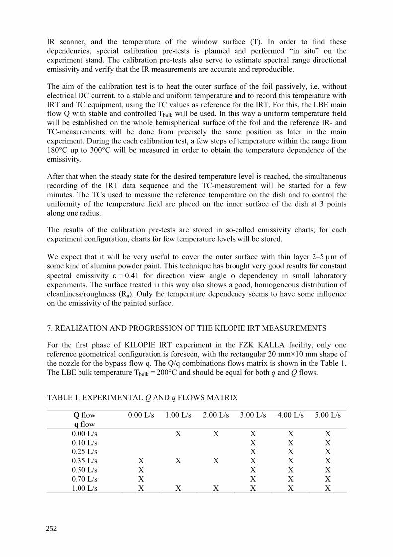
IR scanner, and the temperature of the window surface (T). In order to find these dependencies, special calibration pre-tests is planned and performed “in situ” on the experiment stand. The calibration pre-tests also serve to estimate spectral range directional emissivity and verify that the IR measurements are accurate and reproducible.

The aim of the calibration test is to heat the outer surface of the foil passively, i.e. without electrical DC current, to a stable and uniform temperature and to record this temperature with IRT and TC equipment, using the TC values as reference for the IRT. For this, the LBE main flow Q with stable and controlled Tbulk will be used. In this way a uniform temperature field will be established on the whole hemispherical surface of the foil and the reference IR- and TC-measurements will be done from precisely the same position as later in the main experiment. During the each calibration test, a few steps of temperature within the range from 180°C up to 300°C will be measured in order to obtain the temperature dependence of the emissivity.

After that when the steady state for the desired temperature level is reached, the simultaneous recording of the IRT data sequence and the TC-measurement will be started for a few minutes. The TCs used to measure the reference temperature on the dish and to control the uniformity of the temperature field are placed on the inner surface of the dish at 3 points along one radius.

The results of the calibration pre-tests are stored in so-called emissivity charts; for each experiment configuration, charts for few temperature levels will be stored.

We expect that it will be very useful to cover the outer surface with thin layer 2–5 μm of some kind of alumina powder paint. This technique has brought very good results for constant spectral emissivity ε = 0.41 for direction view angle φ dependency in small laboratory experiments. The surface treated in this way also shows a good, homogeneous distribution of cleanliness/roughness (Ra). Only the temperature dependency seems to have some influence on the emissivity of the painted surface.

7. REALIZATION AND PROGRESSION OF THE KILOPIE IRT MEASUREMENTS

For the first phase of KILOPIE IRT experiment in the FZK KALLA facility, only one reference geometrical configuration is foreseen, with the rectangular 20 mm×10 mm shape of the nozzle for the bypass flow q. The Q/q combinations flows matrix is shown in the Table 1. The LBE bulk temperature Tbulk = 200°C and should be equal for both q and Q flows.

TABLE 1. EXPERIMENTAL Q AND q FLOWS MATRIX

Q flow 0.00 L/s 1.00 L/s 2.00 L/s 3.00 L/s 4.00 L/s 5.00 L/s q flow

0.00 L/s X X X X X 0.10 L/s X X X 0.25 L/s X X X 0.35 L/s X X X X X X 0.50 L/s X X X X 0.70 L/s X X X X 1.00 L/s X X X X X X

252

The foil heating should be used for four different heat fluxes e.g.: q* = 10, 20, 40, 60 W/cm2. The corresponding DC currents will be approx. 11.4, 16.1, 22.8 and 27.9A (see Section 4). In general, a similar procedure will be followed for all geometrical configurations of the KILOPIE IRT experiments and for the pairs from the experiments flow matrix from Table 1.

— The inner geometrical configuration of the flow and three-flange mockup with: alumina painted specimen, power and TC signals measurements cabling and vacuum chamber will be mounted to the loop;

— The loop will be preheated and LBE fulfilled;

— The vacuum in the vacuum chamber and controlling of temperature of the chamber’s wall will be realized;

— Calibration pre-tests will be performed with only the main flow of Q = 1.0 for few temperature levels in the range expected on the surface during the KILOPIE IRT experiments e.g. Tbulk = 180, 200, 250, 300°C;

— The equalization of the bulk temperatures Tbulk for q and Q flows will be realized;

— The desired heat flux level with proper DC current value will be established;

— The joint IRT, TC and DC measurements will be simultaneously started with the triggering device. The recording time for steady state measurements will be 5 minutes. The measurements will be continued for 2 minutes after each switch-off of the heating and the end of the data-taking terminated the experiment.

8. THEORETICAL MODEL FOR EVALUATION OF THE DATA MEASURED IN THE KILOPIE IRT EXPERIMENT

In the convection heat transfer problem with predominate one dimensional heat flux trough a steel wall, the local heat flux q* may be expressed as

( )bulkinnsteel TTq −⋅= .* α (8.1)

where:

*q local heat flux, α local convection heat transfer coefficient,

innsteelT . temperature on the inner flow contact surface of the steel wall,

bulkT bulk temperature of the LBE flow medium.

The set-up of KILOPIE IRT Experiment is based on Eq. (8.2) directly calculated from Eq. (8.1)

( )bulkinnsteel TTq−

=.

*α (8.2)

The LBE bulk temperature bulkT will be directly measured by TC measurement (see Section 3, Fig. 3).

253

The values of desirable heat flux q* are determinated according Eq. 4.1 and Eq. 4.2, and controlled by DC current measurement.

A little more complicated will be determination of the inner wall temperature, innsteelT . . Because IRT can give only the values of the temperature Tout.foil of the outer surface of the heating foil, the problem arises of estimating the difference between this temperature and the temperature Tsteel,inn at the inner surface of the window. This aspect is discussed below. Knowledge of the behavior of ΔTwall = Tout.foil - Tsteel.inn during the KILOPIE IRT experiments is essential for the interpretation of the IRT measurements.

As mentioned in Pt.3 the specimen is surrounded by a vacuum chamber. Therefore only the radiation loss of the energy trough the outer surface of the foil can take place. The temperature Tamb of the wall of the vacuum chamber is controlled during the measurements by a special water channel; a difference between the ambient temperature Tamb and Tout.foil can be kept small, so that the energy radiation flux q*rad can be neglected, especially in comparison with the convective heat flux q*conv on the inner surface of the specimen dish. It therefore can be assumed that the average heat flux on the outer surface is zero. In conclusion, quasi adiabatic boundary conditions can be assumed on the outer surface of the heating foil.

As the wall thickness δ = 0.5mm of the dish is a small fraction of its diameter D = 178 mm, allows the considerations to be made in the context of the 1-D steady-state conduction model for heat flux with thickness in x-direction. This model can be applied to each small local area of the specimen wall because the predominant heat flux is normal to the surface of heated spherical cap. The main aspects of the model are shown in Fig. 7. As was mentioned in Section 4, the conversion from electrical to thermal energy will take place only within the thickness of the heating foil layer of the composite wall of the specimen dish and at a local volumetric rate denoted by qvol. The consequence of this heat generation is that the heat flux is no longer independent of x, and this must be considered in the model calculations.

The small ratio of the thickness δ to the diameter D of the spherical cap dish and as inward convective heat flux perpendicular to the wall predominates, the simple steady-state 1-D model Fig. 7 with uniform energy generation per unit volume in the first heating foil layer of composite wall qvol = constant and constant thermal conductivities kfoil, kepox, kcer, ksteel, through all layers can be used for the plane wall.

The appropriate heat equation for the foil layer is then

0)(2

2

=+foil

vol

kq

dxxTd (8.3)

where:

kfoil - is thermal conductivity of the steel foil, qvol - local energy generation per unit volume.

254

The general solution of equation (8.3) is

212

2)( CxCx

kqxT

foil

vol +⋅+⋅−= (8.4)

The constant of integration C1 = 0 results directly from the assumption of adiabatic boundary conditions (dT/dx)(x=0) = 0 on the outer surface of the mockup, as discussed above. The constant of integration C2 = Tout.foil is directly evaluated from the boundary conditions T(x=0) = Tout.foil , which are known from the IRT measurement. Consequently the temperature distribution is given by Eq. 8.5.

foiloutfoil

vol Tk

xqxT .

2

2)( +

⋅⋅

−= (8.5)

Inserting foilx δ= into Eq.8.5, the temperature epoxfoilx TTfoil .)( ==δ on the inner surface of the

wall is given by Eq.8.6.

foiloutfoil

foilfoilout

foil

foilvolepoxfoil T

kq

Tk

qT ..

2

, 2*

2+

⋅

⋅−=+

⋅

⋅−=

δδ (8.6)

where: volfoil qq ⋅= δ* is the local heat flux, other symbols see Eq. 8.3 and text.

The desired value for ΔTfoil = Tout,foil- Tfoil,epox is then given by Eq. 8.7 .

foil

foilepoxfoilfoiloutfoil k

qTTT

⋅

⋅=−=Δ

2*

,.

δ (8.7)

We can express the local heat flux in dependency of temperature

foil

foil

epoxfoilfoilout

k

TTq

2

* ,,

δ−

= (8.8)

255

�� � �� ��� �� ��� ��� �� !� ��� ��� ��� ����� � ���

� � � & �

�� � � � � �

�� �

, � , 3 4

, � , , 3

, � , 3 , � 3

������������� ������� ���

���5��!������ ���� ��� �67�8

'9��

7

. " �

.� " �

.� � � :

� � � � �

7 ; 4

7 ; <

7 ; 3

7 ; +

7 ; 7

7 ; ;

7 ; ,

7 , =

7 , >

7 ; ?

7 ; >

7 , ?

7 , +

7 , 3

7 , <

7 , 4

7 , 7

7 , ;

7 , ,

. "

� ; ,

� � � �

� � � � � �

5������!��

�������������

�����!��� �

5��6�'$6 @7&#�'$

.� � "

� � � � � � ! � � � � & � � A � 6 � �5 � � �

& � � � � � �

" � � A 6 7 , 8 ' � � 7

,

;

7

4

� ;

� 7

� <

� 3

<

3

+

>

=

; ,

; ;

; 7

� +

� ?

� >

� =

?

.� " � � �

����������� ��

����������������

������������������

: � � � � �

6 ; 4 � = � 8 ' � : �

: � � & �

� 6 ; � 7 > � 8 ' � :

! � � � � � � � � � � � � 5 � �

: �� � � � � �

� 6 3 � ? 7 � 8 ' � :

:� �

� 6 7 > � < 3 � 8 ' � :

� � � �, � 3 3 , � + ,, � , 3 , � ; , , � ; 3 , � 7 ,, � , ,

� 4

FIG .7. KILOPIE IRT; 1-D heat flux model for the multilayer wall of specimen dish with heating foil glued to the T91 steel. An example for approximately numerical values of temperature distribution within the wall. For this simplified calculation following input values are assumed: Tbulk=200°C, heat flux q* = 20 W/cm,2 and heat transfer coefficient a = 2 W/(Kcm2).

Because the heat flux is constant through the specimen wall, and for another layers, i.e. epoxy (glue), ceramic (electrical insulation) and dish steel, linear conduction takes place, the equations for heat flux for each layer expressed in dependency with temperature are:

For the epoxy layer:

epox

epox

cerepoxepoxfoil

k

TTq δ

,,*−

= , (8.9)

256

For the ceramic layer:

cer

cer

steelcercerepox

k

TTq δ

,,*−

= , (8.10)

For the shell dish wall layer:

steel

steel

innsteelsteelcer

k

TTq δ

,,*−

= , (8.11)

finally the same heat flux q* is going by convection to LBE bulk flow from the inner surface of the steel wall of the specimen dish, as it has been mentioned at the beginning of this chapter, see Eq. 8.1.

From Eq.8.8 -8.11 we can reduce all temperatures inside of the specimen wall, therefore

steel

steel

cer

cer

epox

epox

foil

foil

innsteelfoilout

kkkk

TTq

δδδδ+++

−=

2

* ,, , (8.12)

In this place it should be mentioned that the whole expression in denominator of Eq. 8.12 represent a thermal resistance of the multilayer wall for the simplified one-dimensional ideal conduction heat transfer model.

In the fact between the layers some additional so called a thermal contact resistance Rth,c can exist (e.g. see Chapter 3.1.4 and Ref. [7]). Therefore the whole thermal resistance totalthR , of the multilayer wall can be expressed as in Eq. 8.13.

steel

steelsteelcercth

cerl

cercerepoxcth

epox

epoxepoxfoilcth

foil

foiltotalth k

Rk

Rk

Rk

R δδδδ++++++= −−− ,,,,,,, 2

(8.13)

Because in particular the values of the thermal contact resistances between wall’s layers are unknown the total thermal resistance totalthR , can not be calculated only from known thicknesses/bulk conductivities of materials and has to be determined experimentally in a separate subtask of KILOPIE.

Therefore the Eq. 8.12 can be converted to the simple Eq. 8.14, which allows calculating the unknown temperature on the inner surface of the steel dish.

totalthfoiloutinnsteel RqTT ,,, * ⋅−= (8.14)

Finally, putting Eq.8.14 into Eq.8.2 we receive the Eq. 8.15 which allows the determination of the local convection heat transfer coefficientα

257

totalthbulkfoilout R

qTT

,,

*

1

−−

=α (8.15)

expressed with values measured during the KILOPIE IRT Experiment. In particular it should be accentuated, that the temperature values of the outer surface of the heating foil, obtain by IRT, can be used for the determination of the heat transfer coefficientα on the inner surface of the mock-up of the MEGAPIE target window.

9. CONCLUSIONS

1. The previous practical experience with IRT and now new preparation of the specimen heating allow the numerical work out of the 2DD-IRT data to the graphical representation of the local heat transfer coefficient “α”.

2. Preparations of the KILOPIE IRT experiment are completed, from both the hardware and software points of view. The performing of whole KILOPIE experiment, IRT- as well HETSS-part, both at FZK KALLA facility, will be done very likely at the beginning of the year 2004. The complementary KILOPIE investigation at the new two circuits PSI-LBE-Double-Loop will follow at the same year 2004.

REFERENCES

[1] PLATNIEKS, I., et al., Development of HETSS Measurement Procedure for the KILOPIE Experiment, PSI Scientific Report 2002, Vol. III, ISSN 1423-7326, Paul Scherrer Institute, CH-5232 Villigen-PSI, Switzerland (2002) pp. 149–150.

[2] PATORSKI, J.A. et al., Two-dimensional and dynamic method of visualization ofthe flow characteristics in a convection boundary layer using infrared thermography, Journal of Theoretical and Applied Mechanics, Vol. 39, ISSN 1429-2955 (2001)pp. 351–376.

[3] BAUER, G.S., SALVATORES, M., HEUSENER, G., MEGAPIE, a 1 MW Pilot Experiment for a Liquid Metal Spallation Target, J. Nucl. Mat. 296 (2001) pp. 17–35.

[4] DURY, T., Best-estimate fit for MEGAPIE Heat Deposition Profile Data of 19.2.01, PSI Memorandum, 22.03.2001, PSI, CH-5232 Villigen, Switzerland.

[5] PATORSKI, J.A., et al., Experimental estimation of optimum Bypass-jet-flow conditions for the cooling of the window of the SINQ liquid metal target, PSI Report 2000, ISSN 1423-7350, Vol. VI, PSI, CH-5232 Villigen, Switzerland (2000)pp. 42–44.

[6] AGEMA Infrared Sytems, “Thermovision®900 Series User's Manual” AGEMA Infrared Sytems Publication No.556960 (1993).

[7] INCROPERA, F.P., DeWITT D.P., “Fundamentals of Heat and Mass Transfer” (Fourth Editions), JOHN WILEY & SONS, New York (1996).

258

THERMAL-HYDRAULIC ADS LEAD BISMUTH LOOP (TALL) AND EXPERIMENTS ON A HEAT EXCHANGER

B.R. SEHGAL, W.M. MA, A. KARBOJIAN Royal Institute of Technology (KTH), Stockholm, Sweden

Abstract

Royal Institute of Technology (KTH) is participating in two specific research projects of the EURATOM Fifth Framework Programme, one named as TECLA and the other as PDS-XADS, both on Accelerator-driven Transmutation of Waste (ATW) using lead-bismuth eutectic (LBE) as spallation target as well as coolant in a subcritical reactor which is driven by an accelerator. According to the work-package profiles of TECLA and PDS-XADS, the Thermal-hydraulic ADS Lead-bismuth Loop (TALL) was designed and constructed at KTH to investigate the heat transfer performance of different heat exchangers, and the thermal-hydraulic characteristics of natural circulation and forced circulation flow under steady and transient conditions. The specifications of TALL are chosen to simulate prototypic thermal hydraulic conditions of an ADS reactor, with well-conditioned flow and controllable power for thermal-hydraulic tests. The facility is 6.8m tall and the placement of heaters and heat exchangers allows natural convection flows as should occur in the prototypic vessel. The LBE loop is of full height and has been scaled for prototypic (power/volume) ratio to represent all the components. Their LBE volume, pressure drops, flow velocity and heating rates correspond to one tube of the heat exchanger design chosen. The loop is re-configurable for thermal-hydraulic experiments with steady and transient conditions. Sections of the loop allow for easy replacement. The LBE flow and heat transfer characteristics of a straight-tube heat exchanger was presented in the present paper. The heat exchanger has counterflow arrangement, consisting of a pair of 1-meter-long concentric ducts, with LBE flowing in the inner tube of 10 mm ID and the secondary coolant flowing in the annulus.

1. INTRODUCTION

Accelerator-driven systems (ADS) have been proposed for the transmutation of the long-lived actinides in spent nuclear fuel and waste. Lead-bismuth eutectic (LBE) is likely to be a leading candidate for both coolant and target of ADS because LBE has exceptional chemical, thermo physical and neutronic properties well suited for nuclear coolant and spallation target applications [2–6]. In particular, LBE has a low melting temperature (~125°C) and a very high boiling temperature (~1 670°C). It is chemically inert and does not react with air and water violently, and its spallation can yield close to 30 neutrons per 1 GeV proton. However, LBE is not compatible with common steels used in nuclear installations, which therefore requires specific protective means. Due to its high atomic number, the understanding of LBE flow and heat transfer is also necessary for the thermal-hydraulic design of ADS. The project of Technology, Materials and Thermal-Hydraulics for Lead Alloys (TECLA) from European Commission 5th Framework Programme aims to validate the choice of LBE as the spallation material in the target and/or the coolant in a hybrid reactor. The key objective of TECLA is to investigate the corrosion phenomenon of the structural material with LBE and the thermal-hydraulic performance for LBE. Royal Institute of Technology (KTH) participates in the medium-scale experiments of TECLA on heat exchanger and immersion cooler. According to the program of the work-package, the Thermal-hydraulic ADS Lead-bismuth Loop (TALL) was designed and constructed at KTH. The present paper focuses on the description of TALL. The heat transfer characteristics of a straight tube heat exchanger is presented. The heat exchanger has counterflow arrangement, consisting of a pair of 1-meter-long concentric ducts, with LBE flowing in the inner tube of 10 mm ID and glycerol flowing in the annulus. The test matrix variations are as follows:

Inlet temperature: 230 to 450°C Temperature drop: 20 to 100°C LBE velocity: 0.5 to 2.5 m/s

259

The resistance characteristics of a straight tube in the heat exchanger is investigated as well for the LBE flow range: 104 < Re < 105.

2. DESCRIPTION OF TALL TEST FACILITY

Several concepts of ADS have been developed. ASALDO design is one of the reference systems in PDS-XADS. The test facility is mainly referred to the same design.

2.1. Specifications

TALL is a medium-scale facility designed to perform investigation on LBE flow and heat transfer with prototypic thermal-hydraulic conditions (as in conceptual ADS design). The flow can be forced convection or natural circulation in character. TALL can also be used to study the performance of a conceptual design during representative accident scenarios. The current objective of the TALL is to perform experiments for TECLA, i.e. to investigate the heat transfer performance of different heat exchangers. The near-term objective is to investigate the thermal-hydraulic characteristics of LBE natural circulation and forced circulation flow under steady and transient conditions. The specifications of TALL are set and modified to simulate prototypic thermal hydraulic conditions of an ADS reactor, with well-conditioned flow and controllable power for thermal-hydraulic tests. The facility consists of a primary loop (LBE loop) and a secondary loop (oil loop). The LBE loop consists of sump tank, core tank, expansion tank, heat exchanger, EM pump, EM flowmeter, electric heaters and instrumentation. It is 6.8 m tall and the placement of heaters and heat exchangers allows natural convection flows as should occur in the prototypic vessel. Scaling is based on two considerations: resources and conceptual ADS designs. The LBE loop is of full height and has been scaled for prototypic (power/volume) ratio to represent all the components, their LBE volume, and pressure drops, the flow velocity and the heating rates corresponding to one tube of the heat exchanger design chosen. For the final design, the partners and international collaborations provided the needed technological underpinning. The technical parameters are as follows:

─ All parts in contact with LBE are made of 316 or 316L stainless steel, and the internal surfaces are oxidized before filling with LBE;

─ The overall height of the facility is 6.8 m; ─ Total electric power is 55 kW (increasable); ─ LBE flow velocity up to 3 m/s in the heat exchanger; ─ LBE volume flow rate up to 2.5 m3/h; ─ Maximum LBE temperature is up to 500°C; ─ Maximum temperature difference along the heat exchanger is 150°C; ─ The pressure at the top is ~1bar and the bottom pressure is ~8 bar; ─ Maximum natural convection velocity is ≈50 cm/s; ─ The LBE has the composition of 45% Pb and 55% Bi in weight, with the melting point

of 123.5°C; ─ LBE purity is higher than 99.5%; ─ Oxygen level in LBE is measurable; ─ The working fluid in secondary loop is glycerol (C3H5(OH)3) with the boiling point of

290°C; ─ Configuration provides flexibility for different test sections; ─ Data acquisition and control is available.

260

2.2. Main components

TALL is composed of primary loop and secondary loop. The primary loop is a closed LBE loop consisting of a pump, flowmeter, oxygen meter, heaters, piping, heat exchangers, and tanks. In addition, the facility has data acquisition system, oxygen measurement system, cover gas system, vacuum system and exhaust system. The schematic of the facility is depicted in Fig. 1 and the picture is shown in Fig. 2. The LBE operation and main components of the facility are described in detail as follows.

For the first time only, LBE ingots are loaded into the melting tank and heated to 180°C and held 24 hours with argon flushing, then use a scoop (fine mesh stainless steel) to clean the slag off the top of LBE melt till the mirror surface shows, and then the molten LBE is transferred by drainage and argon pressure into the Sump Tank through the filter. During the routine operation, the LBE is melted in sump tank and pressurized to fill the loop with. EM pump is used to circulate the molten LBE through the loop. After leaving the pump, the LBE flows through the core tank and heated by immersion heaters to a specific temperature at the outlet that is connected to a long vertical pipe, through which the LBE keeps traveling up to the expansion tank and then turns to the oxygen sensor and then the heat exchanger where the LBE’s temperature is decreased to a certain value. The LBE leaves the heat exchanger, and keeps flowing down through the EM flowmeter that is placed on the long vertical pipe between the heat exchanger and the pump, finally returns to the pump.

2.2.1. Tanks The melting tank is designed to melt commercial LBE ingots and remove the impurities. It is a round vessel for the preparation of the melt LBE. The internal height of the vessel is 430 mm with the inside diameter of 303 mm. The melting tank was designed so that it can contain 150% of the loop’s total volume and a certain free volume is for cover gas plenum.

The sump tank collects the melt LBE from melting tank before the circulation. It has the same volume and diameter as the melting tank. It is placed under the loop so that it can collect and hold the LBE when the loop drains. An observation window is available on the top of the sump tank. During the operation, the LBE is melted in the sump tank and then transferred by cover gas pressure into the loop.

Two band heaters are employed to melt the LBE in each tank. The heaters are mounted around the outside surface of the vessel and are well insulated. The LBE’s temperature is controlled automatically by the controllable power supply system.

The highest located component of the loop is the expansion tank, which is used to collect the extra LBE from the loop due to heat expansion and balance the pressure variation. All the three tanks mentioned above are made of a 316 stainless steel.

The core tank is one of the complicated components in the loop. It holds the immersion heaters that give the main electric power supply. The core tank was scaled so that it can represent the reactor core of the ANSALDO conceptual design corresponding to one tube of the heat exchanger, especially from the aspects of flow resistance and coolant inventory. Multi-hole plates are placed in the tank in order to increase the flow resistance. The number of the multi-hole plates can be changed in order to obtain the prototypic ratio of the core tank resistance to the loop’s resistance.

261

FIG. 1. Schematic of the TALL test facility.

262

FIG

. 2. T

he p

ictu

res o

f TAL

L.

263

2.2.2. Heat exchanger According to the sub-task of TECLA, thermal-hydraulic performance of different types of heat exchangers will be investigated. As shown in Fig. 3, straight tube and U-tube heat exchangers were designed to perform the TECLA experiments.

(a) Straight tube (a) U- tube

FIG. 3. Schematic of the heat exchangers. The geometrical scaling is done in order to preserve relevant non-dimensional parameters (Re for forced circulation and Gr for natural convection), and also based on the resources (such as laboratory condition, instrumentation and budget). As a result, single tube heat exchangers were employed. Both heat exchangers are composed of an inner tube and an outer duct; with the primary fluid (LBE) flowing in the inner tube and the secondary fluid (glycerol) is flowing in the annulus. For the ease of fabrication, a square duct is chosen as the outer duct of the U-tube heat exchanger.

A 10-mm-I.D. and 1.5-mm-thickness steel tube is used as the inner tube in both the heat exchangers. LBE velocities and Re numbers similar to those in the heat exchanger of the conceptual ADS design are easy to reach in the experiments. The effective lengths of both heat exchangers are 1 meter, which was decided after comprehensive consideration of the inlet/outlet temperature, heat removal capacity, heat flux and flow resistance.

2.2.3. EM pump

The electromagnetic (EM) pump (Fig. 4) provides the driving head for the forced convection flow. The pump uses the system of rotating permanent magnets that can withstand the LBE temperature from 300 to 450°C as in our application. The LBE flows through the channel located in the gap between these magnets. An AC motor is employed to rotate the pump, on the shaft of which two magnetic disks are fixed.

264

FIG. 4. EM pump.

The pump can develop 1.6 bar pressure at the flowrate of 0.6 L/s. Productivity of the pump is controlled by adjusting the rotation speed of the motor using a standard frequency converter.

2.2.4. Secondary loop

As shown in Fig. 1, a secondary loop was designed to realize the heat transfer form LBE to an intermediate fluid, and finally to an oil-water heat exchanger. Glycerol (C3H5(OH)3) is chosen as the working fluid (intermediate fluid) in the secondary loop because it has a high boiling point, 290°C, and well known thermal properties. The glycerol’s boiling point is much higher than the melting point of LBE (125°C), which also can allow a higher operational temperature (≥125°C) so that the solidification of LBE in the heat exchanger is avoidable.

2.2.5. Instrumentation

The EM flowmeter is designed for measuring the flowrate of liquid LBE in a 316 stainless steel pipe with the diameter of 30 mm. The flow meter consists of a sensor, an electronic block and a cable connecting the sensor with the electronic block. The sensor is mounted vertically around the cold leg under the heat exchanger. The signal from the sensor is processed by the electronic block and the reading is shown on a PC monitor. The liquid LBE’s temperature at the sensor can be up to 400°C. The measuring range of the flowmeter varies from 0.01 to 1.0 L/s.

In order to monitor the oxygen level in the LBE, an oxygen measurement system is employed. The system consists of an oxygen sensor (from LANL) and Keithley 6514 Programmable Electrometer an electrometer.

265

A ROSEMOUNT 3051 Pressure transmitter in combination with the1199 Diaphragm Seal System is employed to measure the pressure drop of LBE flow.

Thermocouples, pressure transducers are used to measure the temperature and pressure, respectively. An electrical panel to control all operations of the heaters, pumps and valves are available. Data Acquisition System (DAS) is realized using National Instruments data input instrumentation and a computer program written in LabView. The readings are read through two SCXI-1102 32-channel amplifiers and a 6035E Analogue Input DAQ card.

3. TEST ON THE STRAIGHT TUBE HEAT EXCHANGER

The facility came into operation in September 2003. The heat transfer of a straight tube heat exchanger has been investigated since then. The ranges of main thermal-hydraulic parameters of LBE in the heat exchanger are the inlet temperature from 230 to 450°C, temperature drops from 20 to 100°C, and velocity from 0.5 to 2.5 m/s.

3.1. Preparatory tests

Prior to the heat transfer experiment, lots of preparatory tests were performed, which are concerned with the tightness of the loop, oxidization of the internal surface which contact LBE, handling and circulation of LBE, and commissioning of the instrumentation and data acquisition system.

The oxidization process took 10 days to keep the primary loop heated up to 380°C with slow air flow. After the oxidization, the tightness was checked and reinforced again if necessary, until the pressure loss is less than 3% during 24 hours. Prior to filling of LBE, the loop is evacuated with a mechanical vacuum pump to pressure less than 100 Pa, and then filled with argon gas. Repeat the above procedures 3 times. The argon contains 2% hydrogen. All these measures ensure the oxygen level (1.5×10-7 to 1.85×10-5 wt%) meets the requirement of oxygen control.

3.2. Pressure drop

Flow resistance is one of the important parameters in nuclear reactor design. The total pressure drop may be composed of the gravity pressure drop, frictional pressure drop, local loss and acceleration pressure drops. For single-phase liquid LBE flow, the major flow resistance results from frictional pressure drop. Method for predicting the frictional pressure drop is needed for system design and performance evaluation.

To date, rare frictional pressure drop data existing for LBE are published. In the present research, the frictional pressure drop of LBE flow through the straight tube is investigated, based on the pressure drop measured by a high temperature differential pressure measurement system mentioned above.

For LBE flow in straight tube, the variation of frictional pressure drop with Reynolds number is shown in Fig. 5, on which the pressure drops calculated with the:

266

Moody correlation (1) [1]

⎥⎥⎦

⎤

⎢⎢⎣

⎡⎟⎠⎞

⎜⎝⎛ ++×= −

3/13

Re1002544.21110375.1

df ε (1)

and

Techo et al. correlation (2) [1]

8215.3Re964.1Reln7372.11−

=f

(2)

are also presented. It appears that the present measured values are averagely 15% higher than those from Techo et al. correlation that is for fully developed turbulent flow and smooth surface condition. In our case, the roughness of the surface should be taken into account. For commercial stainless steel tube, if the roughness may be chosen as 0.018 mm, the pressure drop calculated by Moody correlation [1] is illustrated as the dashed line which is in reasonable agreement with the experimental data.

3.3. Heat transfer characteristics

Heat transfer performance of a heat exchanger is another important consideration in the system design. For the purpose of comparison, investigation is or will be carried out on heat exchangers with straight tube or U-tube, respectively. Some results for the straight tube heat exchanger are presented in this paper.

0

10000

20000

30000

40000

50000

60000

70000

10000 30000 50000 70000 90000 110000 130000 150000

Re

Pres

sure

Dro

p (P

a)

Experiment Moody [1] correlationTecho et al. [1] correlation

FIG. 5. Pressure drop of heat exchanger.

267

Enormous theoretical and experimental studies on fluid convection heat transfer have been performed, and many correlations for convection coefficient are available in heat transfer textbook and literatures. Most of them are concerned with constant wall temperature condition or constant heat flux condition. For heat exchanger configuration, the overall heat transfer coefficient is determined with the convection coefficients of hot fluid and cold fluid. In this investigation, it is difficult (if not impossible) to measure the convection coefficients of the hot and cold fluids, since the configuration of heat exchanger does not allow the availability of internal temperature distribution, as well as in many cases neither the constant wall temperature nor constant heat flux exists. As a result, the overall heat transfer coefficient is directly obtained by measured thermal-hydraulic parameters, from which the fluid convection coefficient may be estimated if necessary. The presentation focuses on the overall heat transfer coefficient, which may be concluded by the Eq.(3)

lmTAUq Δ= (3)

where q is the total rate of heat transfer between the LBE and glycerol, A is the heat transfer area, and lmTΔ is the log mean temperature difference which is determined by

[ ]0

0

)()(ln)()(

chLch

chLchlm TTTT

TTTTT

−−−−−

=Δ (4)

where L and 0 designate each end of the heat exchanger, respectively.

Figure 6 shows the overall heat transfer coefficient rises with increasing glycerol velocity, while keeping the LBE velocity and inlet temperature unchanged.

LBE : u=1.5m/s

500

1000

1500

2000

2500

3000

0 5000 10000 15000 20000Re of Glycerol

Ove

rall

Hea

t Tra

nsfe

r C

oeffi

cien

t (W

/m2 .o C

)

Tin of LBE=400 Deg.C Tin of LBE=280 Deg.C

FIG. 6. Effect of glycerol flow on the overall heat transfer coefficient.

268

Two different temperature levels of LBE are investigated. For the low temperature case (the inlet temperature of LBE is 280°C), laminar single-phase flow may take place at the low Reynolds number, which results in a low heat transfer coefficient. But for the high temperature case (Tin,LBE = 400°C), even the glycerol velocity is so low that laminar flow may prevail, the heat transfer coefficient remains higher. This may be that more significant subcooled boiling of glycerol will happen under the high temperature condition, which significantly contributes to the heat transfer performance.

In order to investigate the effect of LBE flow on the overall heat transfer coefficient of the heat exchanger, some tests are operated under constant inlet temperature and velocity for the cold fluid (glycerol). The result is the overall heat transfer coefficient will increase with the increasing LBE Reynolds number (see Fig. 7).

LBE:Tin=280oC, Glycerol: u=3.6m/s, Tin=150oC

500

1000

1500

2000

2500

3000

20000 40000 60000 80000 100000 120000Re of LBE

Ove

rall

Hea

t Tra

nsfe

r C

oeffi

cien

t (W

/m2 .o C

)

FIG. 7. Effect of LBE flow on the overall heat transfer coefficient.

However, the extent of the variation is not so significant, even in a very large Reynolds number range. Obviously, the heat transfer coefficient of secondary (glycerol) flow is much smaller than that of primary (LBE) flow, and hence dominates the determination of the overall heat transfer coefficient.

4. CONCLUDING REMARKS

TALL facility is designed to investigate the thermal-hydraulic performance of heat exchangers concerned with conceptual ADS subcritical reactor design. Two different heat exchangers are designed respectively with straight tube and U tube. The facility is scaled to represent all the components, their LBE volume, and pressure drops, the flow velocity, the heating rates and the height corresponding to one tube of the heat exchanger design chosen. The facility has come into operation since September 2003.

269

─ The loop is well controlled and thermal-hydraulic conditions can be adjusted properly;─ The operational parameters, such as LBE flowrate and temperature level, meet the

design requirement; ─ Pressure drop through the straight tube appears to be higher than that calculated by

Techo et al. correlation (2) for a smooth tube, but in good agreement with thatcalculated by Moody correlation (1) which takes the effect of surface roughness into account;

─ The heat transfer coefficient of secondary (glycerol) flow is much smaller than that ofprimary (LBE) flow, and hence dominates the determination of the overall heat transfer coefficient;

─ At high LBE temperature level, the heat transfer coefficient of glycerol in thesecondary side of the heat exchanger is much higher than that calculated by availablecorrelations. This might mainly results from subcooled boiling of glycerol;

─ More experiments, data check and analysis are to be performed. The test on theU-tube heat exchanger is on the way, which will be used to compare with the straighttube heat exchanger.

REFERENCES

[1] KAKAC, S., et al., Handbook of single-phase convective heat transfer, John Wiley&Sons, New York (1987) pp. 424–426.

[2] CONDÉ, H., (Ed.) Proc. 2nd Int. Conf. on Accelerator-Driven Transmutation Technologies and Applications (ADTT’96), 1996, Kalmar, Sweden, Uppsala University, ISBN 91-506-1220-4 (1997).

[3] GROMOV, B.F., Experience on development of molten lead-bismuth target for accelerator-driven systems, Proc. Conf. on Heavy Liquid Metal Coolants in NuclearTechnology (HMLC’98), 1998, Obninsk, Russian Federation, SSC RF, CRS4, TECH-REP-00/50 (1999).

[4] XADS Pb-Bi cooled experimental accelerator driven system reference configurationSummary report of ANSALDO Nucleare, ADS 1 SIFX 0500-Rev.0 (2001).

[5] Energy amplifier demonstration facility reference configuration, Summary report ofANSALDO Nucleare, EA B0.00 1 200-Rev.0 (1999).

[6] BUONGIORNO, J., et al., Thermal design of lead-bismuth cooled reactors for actinideburning and power production, Massachusetts Institute of TechnologyMIT-ANP-TR-066 (1999).

270

HELIOS FOR THERMAL-HYDRAULIC BEHAVIOR OF PB-BI COOLED FAST REACTOR PEACER

I.S. LEE, K.Y. SUH Seoul National University (SNU), Republic of Korea

Abstract

The liquid-metal-cooled fast reactor PEACER (Proliferation-resistant, Environmental-friendly, Accident-tolerant, Continual-energy, Economical Reactor) is being developed at the Seoul National University (SNU) with the metallic type U-Pu-Th fuel and the lead-bismuth (Pb-Bi) coolant, employing the steam-generating Rankine cycle without an intermediate loop. This work is concerned with the system analysis, pressure drop, natural circulation capacity of PEACER, and a large-scale test loop HELIOS (Heavy Eutectic Loop Integrated Operability & Safety) to support the analysis results for thermal-hydraulic and corrosive behaviour of Pb-Bi. The demonstration loop is being constructed for Pb-Bi natural circulation capability and operating procedure development. Electrically heated rods are used in the heating section and a water-cooling method is adopted in the cooling section. HELIOS has the same elevation, but reduced diameters. The natural circulation potential is a key ingredient of the liquid metal reactor design. PEACER consists of a pool type reactor vessel, which increases the thermal capacity and reduces pressure loss. Under natural circulation condition, flow is driven by buoyancy. In this calculation we followed the single-phase one-dimensional flow loop model.

1. INTRODUCTION

In fast reactors the decay heat is generally removed by the forced convection of the primary coolant pumps. Operation of the primary coolant pumps requires the electric power, which should be supplied by two or four independent trains. However, during a total loss of flow accident, the decay heat must be removed by the natural circulation alone. The primary system coolant was chosen as sodium (Na) in many of the liquid metal reactor (LMR) design. Particularly, the Na coolant has good heat transfer characteristics and high neutron economy.

The risks involving the Na activation and fire, however, have barred the Na cooled LMR from replacing the commercial PWRs. Other candidate materials have been considered for the coolant such as helium, molten salts, lead or lead-bismuth (Pb-Bi) alloy. Pb-Bi has the low chemical activity with air or water. The steam generating system can directly be coupled to the primary liquid metal coolant system without needing an intermediate loop in-between. In particular, Russia has an experience in operating the Pb coolant reactor for military purpose. In utilizing the Pb-bi coolant the pumping work and the structural design require a certain degree of engineering considerations. Pb-Bi also causes chemical corrosion to the structure materials [1].

PEACER is a liquid-metal-cooled fast reactor whose design goals include proliferation resistance, environmental friendliness, accident tolerance, continual energy, and economical reactor. In an earlier study, the conceptual design for PEACER was developed to meet the aforementioned goals. PEACER is being designed with the metallic type U-Pu-Th fuel and the Pb-Bi coolant, but without an intermediate loop. It not only produces power but also transmutes long-term radioactive materials. PEACER can transmute the minor actinides of two pressurized water reactors, 1000 MWe power each. The core design follows the basic Integral Fast Reactor burner of a 1 560 MWth core. It is a pancake type, which increases the neutron leakage and reduces the total fuel volume fraction. It thus increases burning of the transuranic isotopes. The inner reflector also increases the radial neutron leakage. PEACER has a low power density, a large pitch-to-diameter ratio, and a short fuel height design. The fuel assemblies are in a square array, which increases the flow area and the neutron leakage. The grid spacers support the fuel pins. There are two fuel types: inner low enriched fuel, and outer high enriched fuel. Two region configurations flatten the neutron flux. A large-scale loop HELIOS

271

(Heavy Eutectic Loop Integrated Operability & Safety) is being constructed to test the Pb-Bi natural circulation capability and develop the operating procedure. Electrically heated rods will be used in the heating section and a water-cooling method is used in the cooling section.

HELIOS has the same elevation but reduced diameters. General scaling laws for modeling nuclear reactor systems have been proposed in the literature. Most test facilities designs were based on the power-to-volume scaling philosophy. The important requirements for this scaling methodology were described. One of basic doctrines of this scaling methodology is the preservation of the elevation to be the same as that in the prototype. Thus, the test facility has a flow cross-sectional area scaled by the volume-scaling ratio.

2. ANALYSIS OF PEACER SYSTEM

2.1. Thermal efficiency of steam generator

In the PEACER system, the primary loop is directly connected to the secondary loop through two steam generators. The tubes of the steam generator are of the one-through type. The Pb-Bi coolant flows on the shell side, while the water coolant flows on the tube side. Figures 1 and 2 represent the PEACER system and its T-s diagram for the secondary side. The T-s diagram in Fig. 2 illustrates the thermodynamic state of the fluid at various points on the secondary cycle.

FIG. 1. Schematic diagram of PEACER system.

272

FIG. 2. T-s diagram for secondary loop.

The system adopted forced circulation by the main coolant pump (MCP) and the basic Rankine cycle for power generation. The pipes and valves were not considered in this simplified analysis. When there was no feedwater heater, the temperature difference was sizable between inlet and outlet of the steam generator (SG). The thermal expansion of the structural material would be severe in this situation. The steam at the turbine inlet is superheated at 633.15 K and 8 MPa. Steam is extracted from the high pressure turbine (HPT) at 0.345 MPa with quality of 0.855. A moisture separator is installed between the high pressure turbine and the low pressure turbine to minimize erosion of the low pressure turbine (LPT) blades. This cycle is somewhat difficult to show on a T-s diagram since the mass of steam flowing through a series of components vary.

Using the algorithm for the steam generator, thermal efficiency for the cycle at 8 MPa is 36.8% and the electric power is 619 MWe.

A flow chart of the thermal efficiency program for the steam generator is presented in Fig. 3.

273

FIG. 3. Calculation algorithm for steam generator efficiency.

2.2. Pressure drop in reactor core

According to the design of PEACER in 1998, the fuel diameter is 10 mm, and the pitch-to-diameter ratio is 1.46. The fuel assembly is divided into three parts: the lower part representing an axial blanket, the intermediate part an active fuel, and the upper part signifying the fission gas plenum. The temperature distribution in the core was calculated using the energy conservation equation. The fuel pins are assembled in a square array with honeycomb-type grid spacers in the upward vertical channel. Table 1 presents the design parameters for the reactor core.

274

TABLE 1. DESIGN PARAMETERS OF PEACER CORE

Parameter Value

Core pressure, MPa 1

Inlet/outlet temperature, K 300/400

Number of fuel pins 70 588

Core flow rate, kg/s 106 120

Fuel rod outside diameter, cm 1

Fuel rod height, cm 135.3

Active fuel height, cm 50.1

Total power, MWth 1 560

The total pressure drop in the core, excluding the form loss, is divided into three parts: acceleration, friction, and gravity.

PPPP gravfricacc ΔΔΔΔ ++= (1)

where

P accΔ = accelerational pressure drop

P fricΔ = frictional pressure drop

P gravΔ = gravitational pressure drop

In the upward vertical channel, as depicted in Fig. 4, and the steady-state, single-phase liquid flow condition, one may neglect variation in the physical properties along the heated channel, thereby decoupling the momentum equation from the energy equation. If, in addition, the flow area is axially constant, the mass flux is constant. For the case where ρm = ρl ≈ constant, the acceleration pressure drop is negligible. Hence, the governing equation can be approximated as

( ) ( )ZZgZZD

GGfinoutlinout

le

mm

oi PP −+−=− ρρ2 (2)

The PEACER fuel assembly is demonstrated in Fig. 5. To obtain the mass flow rate per unit area the flow area in each sub-channel must first be obtained. The rod-centered cell illustrated in Fig. 5 produces the same results.

275

FIG. 4. Surface heated flow channel. FIG. 5. Representative interior cells in PEACER fuel assembly.

2.3. Pressure drop at spacers

Next calculation deals with the pressure drop at spacers. The spacers are latticed in 196 fuel assemblies with five spacers per assembly, which is of 14×14 rod array. De Stordeur [2] measured the pressure drop characteristics of a variety of spacers and grids as shown in Fig. 6 for the honeycomb spacers. The pressure drop at the spacers of PEACER is correlated in term of a drag coefficient. The pressure drop across the spacer is given by Eq.(3)

⎟⎟⎠

⎞⎜⎜⎝

⎛⎟⎟⎠

⎞⎜⎜⎝

⎛=Δ A

AVcPv

ssss 2

2ρ (3)

The spacer drag coefficient is a function of the Reynolds number for a given spacer type. On the basis of tests of several spacers, Rehme [3] found that the effect of the ratio As/Av is more pronounced than was indicated by De Stordeur [2]. Referring to Fig. 7, Rehme concluded that the spacer pressure drop data are better correlated by Eq.(4)

⎟⎟⎠

⎞⎜⎜⎝

⎛⎟⎠

⎞⎜⎝

⎛=Δ AvAsV v

vs cP2

2

2ρ (4)

2.4. Flow loop analysis

The natural circulation potential is a key characteristic of the LMR design. PEACER consists of a pool type reactor vessel, which increases thermal capacity and reduces pressure loss. Under natural circulation conditions, the flow is driven by the buoyancy. The elevation between the core and the steam generator corresponds to the buoyancy pressure head. Also, the temperature difference between the inlet and outlet produces the coolant density change. In this calculation we followed the single-phase one-dimensional flow loop model due to

276

Todreas and Kazimi [4, 5], and Kazimi [6]. The pressure drop due to buoyancy is given by Eq.(5)

LgTP Ho ΔΔΔ = ρβ (5)

FIG. 6. Drag coefficient for rod bundle spacer [2].

FIG. 7. Modified drag coefficient [3].

277

The density was assumed to vary linearly with the temperature pursuant to the Boussinesq approximation in this calculation. The pressure drop due to friction is written out as:

ρ lR

mCP 2

2

=Δ (6)

)(mRC

n

R

−= (7)

For highly turbulent flow, n = 0.25, and for laminar flow, n = 1. The proportionality constant, R, can be determined from the normal operation condition.

We thus have

ρ l

nmΡ21P 2

2−

=Δ (8)

Combining Eqs (5) and (8) gives the mass flow rate as

⎟⎠⎞

⎜⎝⎛ ΔΔ −

= ρβ 2 )2(1

2o

n

RLgTm H (9)

We can derive the relation among the thermal power, the mass flow rate, and temperature difference. The mass flow rate is determined by the pressure drop. The flow velocity decreases while the pumping power reduces. If the pumping power approaches zero, there is the flow velocity of a natural circulation. We fixed the temperature difference between inlet and outlet. The temperature differences between inlet and outlet under natural circulation condition is greater than about 26°C during the normal operating condition. The elevation of 8 m between the thermal centers of the core and the steam generators can remove as much as 10% of the normal operating power when the flow is turbulent.

3. HELIOS EXPERIMENTAL STUDY FOR Pb-Bi EUTECTIC

Figure 8 demonstrates the schematic diagram of the HELIOS demonstration loop.

278

FIG. 8. Schematic diagram of HELIOS.

3.1. Scaling of demonstration loop

HELIOS demonstration loop is being designed for Pb-Bi natural circulation capability and operating procedure development. An electric heating rod will be used in the heating section and an oil cooling method will be used in the cooling section of HELIOS. The scaled test facility will be constructed to natural circulation behavior in a prototype plant, PEACER. HELIOS has the same elevations and the reduced diameters. General scaling laws for modeling nuclear reactor systems have been proposed by Ishii and Kataoka [7]. Most of the test facility designs were based on the power-to-volume scaling methodology. The important requirements for this scaling methodology were described by Zuber [8] and Karwat [9]. One of basic doctrines of this scaling methodology is preservation of the elevations between the model and the prototype. Thus, the test facility has a flow cross-sectional area scaled by the volume scaling ratio. Heisler [10] and Ishii and Kataoka [7] made an attempt to develop scaling laws for the natural circulation loops. Ishii and Kataoka method is adopted to design the HELIOS demonstration loop.

In this analysis, subscripts 0 and r denote the reference constant value and representative variable of a system. The i th component and solid are denoted by subscripts i and s. Using the Boussinesq assumption for a single phase natural convection system, the fluid is considered incompressible, except in the gravitational term in the momentum equation. Then the conservation laws can be expressed by the following set of simplified balance equations based on a one-dimensional formulation:

Continuity equation

Integral momentum equation

OCS

Mockup Core Pb-Bi Pump

SG

Pb-Bi

Freezing Valve

300℃, 6.83 kg/s

400℃, 6.83 kg/s

Instrumentation

Orifice Flowmeter Temperatur

e Flow

Orifice Flowmeter

Main Loop & Storage

OCS

Solid HeaterMelt & Storage

Tank

279

∑∑ ⎟⎟⎠

⎞⎜⎜⎝

⎛⎟⎠

⎞⎜⎝

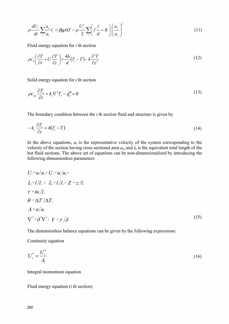
⎛+−Δ=

i i

o

i

r

ii

i

or

aa

Kdl

fU

Tglaa

dtdU

22

2ρρβρ (11)

Fluid energy equation for i th section

( ) 2

24zTkTT

dh

zTU

tTc sp ∂

∂−−=⎟

⎠⎞

⎜⎝⎛

∂∂

+∂∂ρ (12)

Solid energy equation for i th section

02 =′′′−∇+∂∂

ssss

ps qTkt

Tcρ (13)

The boundary condition between the i th section fluid and structure is given by

( )TThyTk s

ss −=∂∂

− (14)

In the above equations, ur is the representative velocity of the system corresponding to the velocity of the section having cross sectional area ao, and lh is the equivalent total length of the hot fluid sections. The above set of equations can be non-dimenzionalized by introducing the following dimensionless parameters:

uuU oii= , uuU orr

= ,

llL oii= , llL ohh

= , lzZ o=

ltu oo=τ

TT oΔΔ=θ

aaA oii=

∇∇ =222* δ , δyY = (15)

The dimensionless balance equations can be given by the following expressions:

Continuity equation

i

ri A

UU*

* = (16)

Integral momentum equation

Fluid energy equation (i th section)

280

( )i

iisii

i

i

ri

PeSt

ZAU θθθθ

τθ

−−=∂∂

+∂∂ *

(18)

Solid energy equation (i th section)

02** =−∇+∂∂

sisiisi QTt

θθ

(19)

Fluid-solid boundary condition (i th section)

( )isiis B

Yθθθ

−=∂∂

(20)

The similarity groups appearing in the above equations are defined as:

Richardson number

forceinertiabouyancy

UlTgRi

o

oo

2 =Δ

=β

(21)

and

Friction number

( ) forceinertiafriction

Kdfl

iFi

=+= (22)

In addition to the above defined physical similarity groups, several geometrical similarity groups are obtained. These are:

Axial scale

llL oii= , llL ohh

=

and

Flow area scale

aaA oii=

281

The similarity criteria between two different systems can be obtained from a detailed consideration of the similarity groups developed above together with necessary constitutive relations. In the following analysis, subscript R denotes the ratio between the model and prototype. Thus,

prototypefor modelfor

ψψ

=≡ψψψ

p

m

R

(23)

Table 2 shows the material properties of Pb-Bi in this analysis. The properties are referenced from Chu et al.’s report [11].

TABLE 2. MATERIAL PROPERTIES OF PB-BI [1]

Parameter Pb-Bi

Composition, weight, % 44.5% Pb 55.5% Bi

Melting point, °C 125

Density, kg/m3 10 240

Volumetric thermal expansion coefficient, K-1 2.2×10-5

Thermal conductivity, W/mK 11.9 Specific heat, J/kgK 146.4

Kinematic viscosity, m2/s 1.5×10-7

Viscosity, Pa s 0.00166 Pr 0.019

Table 3 presents typical thermal-hydraulic design parameters of PEACER.

282

TABLE 3. DESIGN PARAMETERS FOR 1 560 MWth PEACER [1]

Core

Fuel pin diameter, mm 10.0

Pitch-to-diameter ratio 1.46

Active fuel height, m 0.501

Total fuel height, m 1.353

Core diameter, m 4.896

Total 732

Fuel 360

Inner core 184

Outer core 176

Inner radial reflector 32

Outer radial reflector 100

Radial shield 192

Assembly

Control/shutdown 20

Inner core 196 (14×14) Fuel pin per assembly Outer core 196 (14×14)

Flow area at the core, m2 9.50538

Hydraulic diameter at the core, mm 17.13

Projected frontal area of the spacer, m2 4.37297

Steam generator (SG)- 2 loops

Number of secondary tube 17 965

Outer diameter of secondary tube, mm 20.3835

Hydraulic diameter of SG, mm 26.39

Flow area at SG, m2 15.27025

Projected frontal area of the spacer, m2 4.37297

Diameter of hot leg and cold leg, m 2

8

283

Table 4 presents the loss coefficients used in this analysis. The resistance coefficients for form losses are referenced from Crane [12] and Idelchik et al. [13]. The used equivalent diameter of the prototype is the same value of the hot leg pipe diameter (2 m) in PEACER.

TABLE 4. LOSS COEFFICIENTS IN THIS ANALYSIS

Paramater Loss coefficient (K)

From cold leg to core inlet 1.0

Core inlet 0.3727

Core outlet 0.7454

From core outlet to hot leg 0.5

From hot leg to SG 1.0

SG inlet 0.4187

SG outlet 0.8375

From SG to cold leg 0.5

Elbow (4 EA) 20.0 feq

Pump 4.0

Grid spacer (core: 5EA, SG: 10 EA) Rehme’s data [3]

Figure 9 shows the schematic diagram of HELIOS.

Heater

Cooler

Pump

EMFlowmeter

FIG. 9. Schematic diagram of HELIOS.

284

It has the same thermal center difference with much reduced diameters. Thus, the fraction of wall friction loss at HELIOS is much larger than that at PEACER.

Table 5 shows the results of natural circulation capability from the core of the PEACER. The heated power of prototype is about 10% of thermal power of PEACER. The total circulation length of HELIOS is assumed to 20 m. This analysis provides the important data for determination of the heating and pumping power in the heating section.

TABLE 5. NATURAL CIRCULATION CAPABILITY OF THE PEACER

Parameter Results

Decay heat, MW 156.14

Natural circulation flow rate, kg/s 8710.0

Temp. difference between hot leg and cold leg, K

126.2478

Equivalent flow length, m 5441.342

Flow velocity at pipe, m/s 0.1357350

Re at pipe 1 670 169

Friction factor at pipe 8.73453E-3

Richardson number 11.88189

Total loss coefficient 23.76

The most fundamental requirement for the similarity is concerned with the Richardson number, friction number and geometrical similarity criteria.

The scaling results of HELIOS are

8125.08/5.60.1 === RR HRi (24)

RRRRRR AHQTHu 5.05.0 1, === (25)

3.2. Demonstration loop description

Using the upper scaling results, HELIOS will be designed. The test loop consists of a heating section, a heat exchange with condenser, an electromagnetic pump, a data acquisition system and instrumental device such as electromagnetic flow meter, a pressure gage, and thermocouples.

The dimension of the loop is 5.08 cm (2 inches) in diameter, 6.5 m in height (from bottom to top), and 3.5 m in width (from left to right). The electric heater is cylindrical shape with a

285

surface loading of 400 W/in2. The coolant of a heat exchanger is a mineral oil, which is supplied with a water storage tank.

The test will consist of the pre-test with a water coolant and the test with a liquid metal coolant. When the working fluid is a liquid metal, the corrosion problem must be considered in building the test loop.

The operation temperature of the coolant is about 300~400°C. It is important that the whole surfaces of the test loop should be covered with insulation fiber during the natural circulation test.

Also, using the CAD system such as Pro-E, CATIA, Solidwork, etc, HELIOS is created by the digital mockup exported from a 3D CAD system in the 1:1 scale. These digital mockup products can be analyzed with the general computational analysis code such as CFX and ANSYS with respect to flow behaviour, stress and vibration.

4. RESULTS

Table 6 lists the inlet and outlet temperatures calculated using the energy balance equation, and the thermal efficiency for the steam generator spanning from 5 to 15 MPa.

TABLE 6. TEMPERATURE AND THERMAL EFFICIENCY FOR STEAM GENERATOR

Pressure

(MPa)

Superheated temperature

(°C)

Saturated temperature

(°C)

Sub-cooled temperature

(°C)

Efficiency

(%)

5 360.15 264.06 214.33 32.69

6 360.15 275.70 208.96 34.31

7 360.15 285.94 203.43 35.69

8 360.15 295.12 197.44 36.78

9 360.15 303.46 191.02 37.73

10 360.15 311.11 184.13 38.52

11 360.15 318.20 176.69 39.19

12 360.15 324.80 168.58 39.77

13 360.15 330.98 159.68 40.19

14 360.15 336.79 149.72 40.60

15 360.15 342.28 138.48 40.66

The pressure drop at the spacers of PEACER is calculated using Rehme’s model, which leads to a lower pressure drop. Table 7 presents the temperature and pressure drop results from the single channel analysis.

286

TABLE 7. SINGLE CHANNEL ANALYSIS RESULTS FOR PEACER

Parameter Results

Inlet/outlet temperature, °C 300/400

Mass flow rate, kg/s 106 120

Active fuel height, cm 50.1

Friction pressure drop, MPa 0.00825

Acceleration pressure drop, MPa 0

Gravity pressure drop, MPa 0.135

Grid spacer pressure drop, MPa 0.0385

Total pressure drop, MPa 0.18175

Figure 10 shows the decay heat fraction that can be removed by the natural circulation due to the distance between thermal centers and the temperature difference.

FIG. 10. Natural circulation heat removal capacity.

The elevation of 8 m between the thermal center of the core and steam generators can remove as much as 10% of the normal operating power when the flow is turbulent. Figure 11 and Table 8 present the results of the flow loop analysis.

287

Based on the result, we calculated the heat removal fractions of different cases. Figures 11 and 12 depict the fractional heat removal according to thermal center difference.

FIG. 11. Heat removal according to thermal center difference.

FIG. 12. Heat removal according to thermal center difference.

288

TABLE 8. NATURAL CIRCULATION IN PEACER

Parameter Full power

Natural circulation

Pressure (MPa) 1 1

Hydraulic resistance - 16.61

T outletinletΔ /(K) 100 126.5

Mass flow rate (kg/s) 106 120 8710.0

Power (MWth) 1 560 156.14

As the thermal center difference increases, the amount of heat removal rises. Turbulent flow is more effective in heat removal than laminar flow as expected. The increment of temperature difference between the inlet and the outlet makes density change, which supplies pressure head for the natural circulation.

Generally the temperature difference exceeds 100K in turbulent flow regime for decay heat removal as shown in Figs 13 and 14, respectively. In Fig. 14 large thermal center difference and high temperature difference produce excessive natural circulation effect.

FIG. 13. Heat removal according to temperature difference.

289

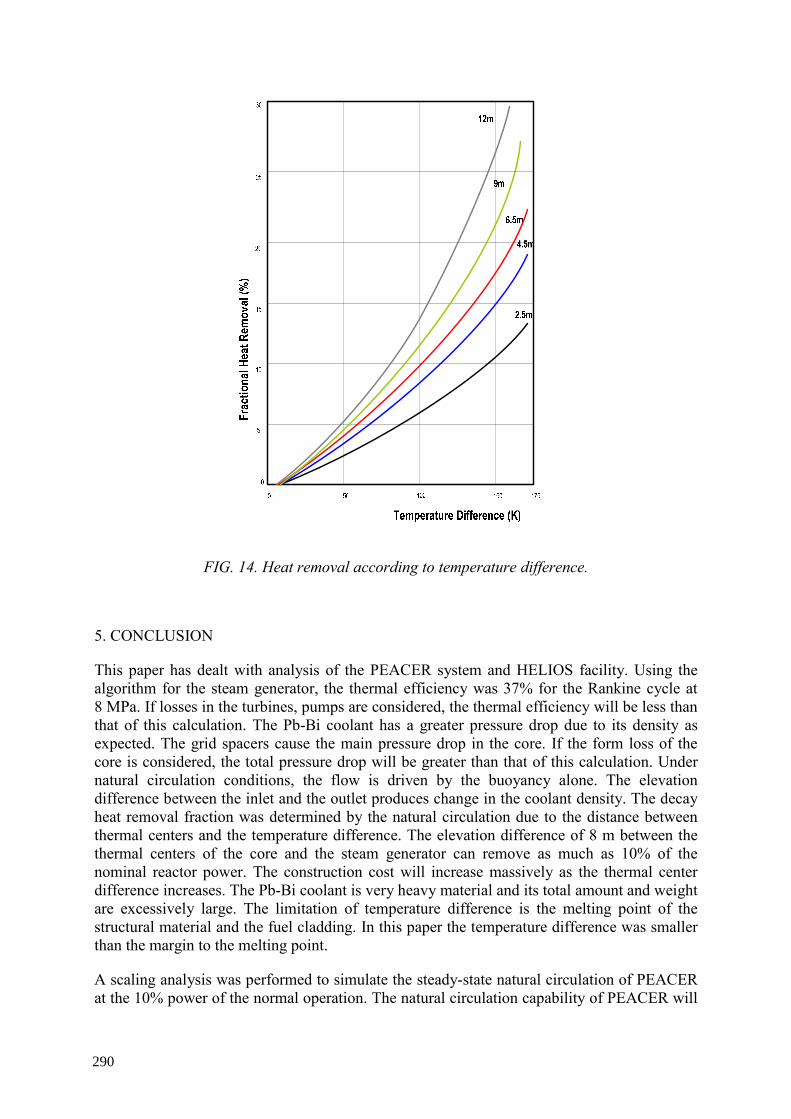
FIG. 14. Heat removal according to temperature difference.

5. CONCLUSION

This paper has dealt with analysis of the PEACER system and HELIOS facility. Using the algorithm for the steam generator, the thermal efficiency was 37% for the Rankine cycle at 8 MPa. If losses in the turbines, pumps are considered, the thermal efficiency will be less than that of this calculation. The Pb-Bi coolant has a greater pressure drop due to its density as expected. The grid spacers cause the main pressure drop in the core. If the form loss of the core is considered, the total pressure drop will be greater than that of this calculation. Under natural circulation conditions, the flow is driven by the buoyancy alone. The elevation difference between the inlet and the outlet produces change in the coolant density. The decay heat removal fraction was determined by the natural circulation due to the distance between thermal centers and the temperature difference. The elevation difference of 8 m between the thermal centers of the core and the steam generator can remove as much as 10% of the nominal reactor power. The construction cost will increase massively as the thermal center difference increases. The Pb-Bi coolant is very heavy material and its total amount and weight are excessively large. The limitation of temperature difference is the melting point of the structural material and the fuel cladding. In this paper the temperature difference was smaller than the margin to the melting point.

A scaling analysis was performed to simulate the steady-state natural circulation of PEACER at the 10% power of the normal operation. The natural circulation capability of PEACER will

290

be demonstrated from this experimental loop. Its transient temperature and flow velocity data are useful to test the predictability of thermal-hydraulic code for PEACER design. In addition, this experimental loop will provide the basic data for the operating procedure development. In the future, the heat transfer coefficient with various flow conditions will be measured in HELIOS. Testing temperatures and flow velocities will be determined after detailed parametric study of the PEACER conceptual design.

GREEK LETTERS

β Volumetric thermal expansion coefficient of Pb-Bi δ Conduction thickness ΔL Between the thermal center of the core and the steam generator ΔT Temperature difference between inlet and outlet θ Non-dimensional temperature μ Viscosity of Pb-Bi τ Non-dimensional time ρ Density of Pb-Bi

SUBSCRIPT

I i th section O Reference constant R Representative variable S Solid H Hot C Cold R Model-to-prototype ratio (…)m Model (…)p Prototype

291

NOMENCLATURE

A Flow area as Wall cross sectional area A Non-dimensional area As Projected frontal area of the spacer Av Unrestricted flow area away from the spacer Bi Biot number Cps Solid heat capacity Cs Modified drag coefficient Cv Modified drag coefficient CR Hydraulic resistance coefficient D Hydraulic diameter De Equivalent diameter F Friction factor F Friction number G Gravitational acceleration Gm Mass flux H Heat transfer coefficient H Thermal center difference of prototype K Orifice coefficient L Axial length lh Length of hot fluid section P Pressure Ps Pressure at spacers q” Heat flux Qs Heat source number Ri Richardson number R Proportionality constant Re Reynolds number T Time T Temperature of Pb-Bi To Reference temperature of Pb-Bi Ts Solid temperature T* Characteristic time ratio U Velocity U Dimensional velocity Vs Velocity in the spacer region Vv Average bundle fluid velocity W Mass flow rate Y Transverse distance Y Non-dimensional axial distance Z Axial distance

292

REFERENCES

[1] CHANG, J.E., Natural Circulation Heat Removal Characteristics of the Liquid Metal Coolant, M.S. Thesis, Department of Nuclear Engineering, Seoul National University, Seoul, Republic of Korea (2000).

[2] DE STORDEUR, A.M., Drag Coefficients for Fuel Elements Spacers, Nucleonics, 19:74 (1961).

[3] REHME, K., Pressure Drop Correlations for Fuel Elements Spacers, Nuclear Technology, 43:17 (1973).

[4] TODREAS, N.E., KAZIMI, M.S., Nuclear Systems I Thermal Hydraulic Fundamentals, Hemisphere Publishing Co., New York, NY, USA (1990) pp. 382–406.

[5] TODREAS, N.E., KAZIMI, M.S., Nuclear Systems� Elements of Thermal Hydraulic Design, Hemisphere Publishing Corp., New York, NY, USA (1990) pp. 73–92

[6] KAZIMI, M.S., et al., A Condensed Review of the Technology of Post-Accident Heat Removal for the Liquid Metal Fast Breeder Reactor, Nuclear Technology (1978).

[7] ISHII, M., KATAOKA, I., Scaling laws for thermal-hydraulic systems under single-phase and two-phase natural circulation, Nuclear Engineering and Design, 81, 411 (1984).

[8] ZUBER, N., Problems in Modeling of Small Break LOCA, Report NUREG-0724 (1980).

[9] KARWAT, H., Principal characteristics of experimental simulators suitable for SBLOCA events of LWRs and scaling principles adopted in their design, Proc. Spec. Meet. Small Break LOCA Analysis in LWRS, Pisa, Italy, 23–27 June 1985, p. 399.

[10] HEISLER, M.P., Development of scaling requirements for natural convection liquid-metal fast breeder reactor shutdown heat removal facilities, Nuclear Science and Engineering, 80, 347 (1982).

[11] CHU, H.S., KIM, C.S., SUH, K.Y., Analysis and experiment for natural circulation in the liquid metal reactor PEACER, Intl Congress on Advanced Nuclear Power Plants (ICAPP), Hollywood, FL, USA, 9–13 June 2002, ICAPP-1086 (2002).

[12] Flow of Fluids through Valves, Fittings, and Pipe, Crane Co., New York, NY, USA (1985).

[13] IDELCHIK, I.E., MALYAVSKAYA, G.R., MARTYNENKO, O.G., FRIED, E., Handbook of Hydraulic Resistance, 2nd edition, Hemisphere Pub. Corp., New York, NY, USA (1986).

293

VOID-FRACTION MEASUREMENTS IN TWO-PHASE NITROGEN-MERCURY FLOWS

P. SATYAMURTHY, N.S. DIXIT Bhabha Atomic Research Centre (BARC), Mumbai, India

P. MUNSHI Indian Institute of Technology, Kanpur, India

Abstract

Gas driven circulating spallation targets and reactor coolants based on high-density molten liquid metals like lead and Lead-Bismuth-Eutectic (LBE) have been proposed recently. To design these systems, it is required to understand two-phase flows under various regimes and develop suitable CFD codes, which have to be properly bench marked. The two-phase flow regimes (bubbly, Churn, Slug) are governed by void fraction distribution and the accurate measurement of void fraction in these systems is complicated in view of high-density and opacity. A mercury facility has been set up to study two-phase nitrogen and mercury flows at ambient temperature. The flow circulation is achieved by creating two-phase flow in the riser. The flow regime obtained in the facility (bubbly and Churn) is similar to the flows expected in the gas-driven spallation targets. Both single beam and 7-beam gamma ray systems have been developed for void fraction measurement based on high-energy gamma rays. Suitable MART (Multiplicative Algebraic Reconstruction Technique) algorithms have been developed to reconstruct the void distribution based on the measured line averaged void-fraction. Void-fraction distribution is obtained for a typical flow conditions.

1. INTRODUCTION

High-density liquid metals like lead, Lead-Bismuth-Eutectic (LBE) and mercury have been proposed as spallation target for intense neutron source [1]. One of the options to circulate liquid metal is by injecting suitable gas at the entrance of the riser [2, 3]. Gas driven reactor coolant based on LBE/lead have also been proposed [2]. The main advantage of these systems as compared to liquid metal pumps arises due to its simplicity, less maintenance and ease of operation.

To design these systems, it is required to understand two-phase high-density flows in the riser of the loop under various regimes and develop suitable CFD codes, which are to be validated with experimental data. The two-phase flow regimes (bubbly, Churn, Slug) are governed by void fraction distribution and the accurate measurement of void fraction in these systems is complicated in view of high-density and opacity.

Void fraction in liquid metal flows can be measured by intrusive probes based on electromagnetic principle (potential, micro-magnetic) and opto-mechanical principle [4, 5] or by non-intrusive methods using Gamma rays for high density [6] and X-rays for low-density systems [4].

Non-intrusive probes have the advantage of being used under all process conditions (high temperature, corrosive fluid, etc.) and do not interfere with the flow system. In this paper, details of high-energy gamma-ray attenuation system developed to measure two-dimensional void distribution in the nitrogen-mercury flow based on:

(i) Single-detector parallel beam; and

(ii) Seven-detector fan-beam systems are presented.

295

2. EXPERIMENTAL FACILITY

A 6.5 m high mercury facility has been set up in our institute to study two-phase nitrogen and mercury flows at ambient temperature. The flow is upward and co-current. The flow circulation is achieved by creating two-phase flow in the riser. The flow regime obtained in the facility (bubbly and Churn) is similar to the flows expected in the gas-driven spallation targets. The loop consists of mixer, riser pipe (internal diameter 79.0 mm), separator, downcomer etc. Nitrogen is introduced through the mixer at ~6 kg/cm2 pressure. A two-phase mixture is established in the riser, which gives rise to density difference between the riser and downcomer leading to the circulation of liquid metal in the loop. Nitrogen is separated and is let out to the ambient. Mercury alone flows through the downcomer. A maximum of 60 kg/s mercury flow rate has been achieved. Void fraction is measured using Fan beam gamma ray source at 1.2 m from the mixer and with single beam parallel chords at 2.9 m from the mixer (photograph of the facility is shown in Fig. 1).

FIG. 1. Mercury-nitrogen liquid metal MHD experimental facility at BARC.

296

2.1. Single beam gamma ray system

Single beam gamma ray system is located at 2.9 m above the mixer. The photograph of this system is shown in Fig. 2.

FIG. 2. Photograph of parallel and rotational single beam scanning gamma ray system (60Co of 50 mCi).

The gamma ray source having 3mm window for the beam along with the detector system was installed on a horizontally movable-and rotating platform. 60Co of activity 50 mCi was used as gamma ray source and 1.33 MeV photons were chosen for measurements. NaI (Th) detector (located at a distance 225 mm from the source) with PMT, Pre-amplifier etc. are mounted along with source to collect the projection data from single gamma ray beam. The measurements were taken at 14 chord lengths (parallel to one another by moving source and detector) at a given orientation when the pipe was filed with mercury, when empty and during two-phase flow. This was repeated for every 30° of rotation covering 180° (6-views). One set of experiment generated 84 line averaged void fraction values for the given flow conditions.

297

2.2. Fan-beam gamma ray system

Fan-beam gamma ray system is installed at distance 1.2 m from the mixer. 60Co of 100 mCi gamma ray source is housed in an appropriate lead container. The radioactive source container consists of three lead blocks with one blind, the second one with 7 windows each of 3 mm diameter and the third housing the source, which can be moved in front of the window to obtain fan beam. NaI (Th) detectors (located at a distance 725 mm from the source) with PMT, Pre-amplifier etc. are mounted along with source to receive fan beam gamma rays (the angle between two adjacent rays is 3.5° and equally spaced from the centre line). These rays pass through various chords of the flow in a circular pipe on a rotating platform. Gamma ray attenuation was measured along the 7 chord lengths for every 10° interval up to 170°, when the pipe was filed with mercury, when empty and during two-phase flow. Based upon this data, void distribution was determined with appropriate reconstruction algorithms. 1.33 MeV beam of photons was chosen for these measurements. One set of experiment generated 126 line averaged void fraction values for given set of flow conditions. The photograph of Fan-beam gamma ray system is shown in Fig. 3.

FIG. 3. Photograph of the multi detector high energy gamma ray system for the measurement of void distribution.

298

3. EXPERIMENT

Experiments were carried out for 4.7 g/s flow rate of nitrogen with corresponding 43.0 kg/s flow rate of mercury. Photon counts for each measurement were taken in excess of 3 000 to reduce the Poisson corruption [7]. The size of the gamma ray beam was chosen to be 3 mm so that the error due to finite beam size was negligible [8].

3.1. Determination of line averaged void fraction

From the measured data, the line averaged void fraction, iα for each ray was obtained from the following relation.

( ) ( )ligi

li

tii NNlnNNln=α (1)

Where N corresponds to the number of photon counts per unit time, superscripts t, l, and g correspond to two-phase flow, mercury alone and nitrogen alone and subscript i represents ith ray.

3.2. Multiplicative Algebraic Reconstruction Techniques (MART)

We have studied in detail many variants of MART algorithms (GBH, GH, Lent etc) for reconstruction of void fraction distribution [9]. Here we are presenting the results of Gordon Bender Herman MART (GBH-MART) [10]. In all these methods, the flow region is divided in to square cells and void-fraction is assumed constant within the cell. Void fraction is assumed zero in all those cells, which are outside the flow region. Schematic of the discretization of the physical domain has been presented in Fig. 4.

NDetector

Source Wi,j

1 2 3

ith ray

FIG. 4. Discretization of two-phase flow field.

299

The length of intersection of ith ray and jth cell, denoted by Wi,j (for I = 1, 2 …M and j = 1, 2 ...N) represents the contribution of jth cell to the total void fraction along the ith ray. By accounting the contribution of each cell into the average void fraction along a ray, the result in a system of linear equations is as shown in Eq. (2).

( ) ∑ α⎟⎟⎟⎟

⎠

⎞

⎜⎜⎜⎜

⎝

⎛

∑=α

=

=

N

1jiN

1kk,i

j,iexpi

w

w (2)

From the given Wi,j and measured line averaged void-fractions (left hand side of the above equation) the αis are determined. The different MART algorithms essentially vary in method of updating the new values of void-fraction in each cell. In the case of GBH-MART the updating of void-fraction values are carried as shown in Eq. (3):

( )( )∏ ⎥

⎦

⎤⎢⎣

⎡⎟⎟⎠

⎞⎜⎜⎝

⎛α

α−λ−×α=α

=

cjM

1i theo

expoldj

newj 11 (3)

Here, the Mcj refers to number rays passing through the jth cell. ( )theoiα is the calculated line averaged void fraction of ith ray based on the estimated void fractions in the cells passing through ith ray. The iteration is continued until the required convergence is obtained. λ is the relaxation parameter and the range of its value for convergence of the solution for GBH-MART vary in the range of 0.01 to 0.02. In general it depends on the distribution to be reconstructed.

4. ANALYSIS OF GBH-MART WITH SIMULATED VOID FRACTION

In order to verify the reconstructive capability of GBH-MART, we have studied the reconstruction of this algorithm on a simulated void-fraction configuration as shown in Fig. 5a. For this simulation we have taken 61 rays and 12 angles. As can be seen the reconstruction by GBH-MART (see Fig. 5b) is quite good. The average value is very nearly same as original value. However the reconstructed void-fraction predicts marginally higher void fraction in the outer zone (0.85 as against 0.8) and lower values in the inner core.

300

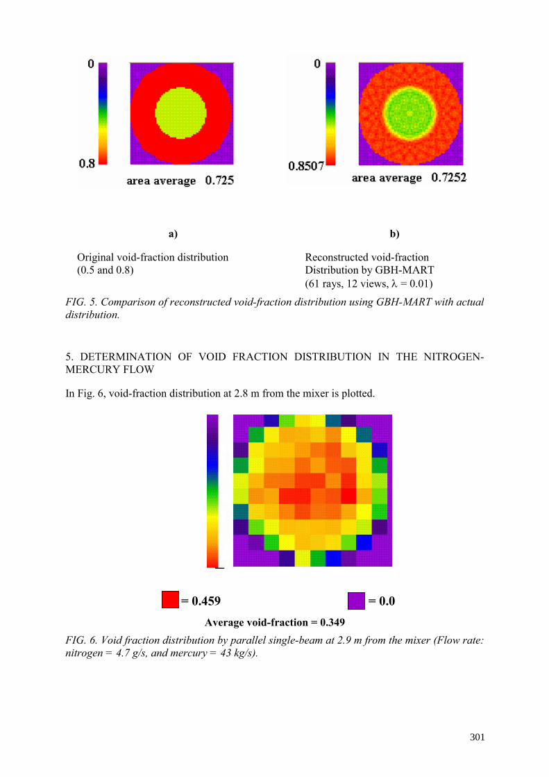
a) b)

Original void-fraction distribution Reconstructed void-fraction (0.5 and 0.8) Distribution by GBH-MART

(61 rays, 12 views, λ = 0.01)

FIG. 5. Comparison of reconstructed void-fraction distribution using GBH-MART with actual distribution.

5. DETERMINATION OF VOID FRACTION DISTRIBUTION IN THE NITROGEN-MERCURY FLOW

In Fig. 6, void-fraction distribution at 2.8 m from the mixer is plotted.

= 0.459

= 0.0

Average void-fraction = 0.349 FIG. 6. Void fraction distribution by parallel single-beam at 2.9 m from the mixer (Flow rate: nitrogen = 4.7 g/s, and mercury = 43 kg/s).

301

The maximum value of the void-fraction was obtained at the central region with a value of 0.46 and the lower value near the wall region. The average value across the cross-section comes out to be 0.35. As expected the flow is essentially approaching the fully developed flow [11].

The measured void distribution using fan beam system for the same flow rates at the location 1.1 m from mixer exit is shown in Fig. 7.

= 0.578

= 0.0

Average Void-fraction = 0.175 FIG. 7. Void fraction distribution by fan-beam at 1.2 m from the mixer (Flow rate: nitrogen = 4.7 g/s, and mercury = 43 kg/s).

The average value obtained was 0.175. We can also see from the figure that overall the void-fraction is much lower as compared to upper location for the same flow rate. This is due to higher pressure at this location leading to higher gas density. Further we see that highest void-fraction obtained was 0.578 in one cell. This value may be spurious due to limitation of number of rays. This has to be further analyzed.

6. CONCLUSIONS

Accurate prediction of void-fraction enables to design gas driven target and reactor circulating systems with optimum gas flow (argon or helium) configuration. In addition, detailed void-fraction distribution enables the estimation of amount of gas that will be carried in to the proton beam pipe in the case of windowless target configuration (Carry-under phenomena). In view of non-intrusive method, high-energy gamma-ray attenuation technique is ideal for measurement of void fraction distribution in high-density two-phase liquid metal flows.

302

REFERENCES

[1] BAUER, G.S., Physics and technology of spallation neutron sources, Nuclear Instruments and Methods in Physics Research A 463 (2001) pp. 505–543.

[2] ENERGY AMPLIFIER DEMONSTRATION FACILITY REFERENCE CONFIGURATION, Summary Report, ANSALDO, EAB0.00 1200-Rev.0, Italy (January 1999).

[3] SATYAMURTHY, P., BISWAS, K., Design of a LBE spallation target for fast-thermal accelerator driven sub-critical system (ADS), paper presented in the 7th

Information Exchange Meeting, Jeju, Republic of Korea, 14–16 October 2002. [4] ECKERT, S., GERBETH, G., GUTTEK, B., STRECHEMESSER, H., LIELAUSIS,

O., Investigations of liquid metal two-phase flow characteristics by means of local resistivity probes and X-ray screening techniques, paper presented in the International Workshop on Measuring Techniques for Liquid Metal Flows, Rossendorf, Germany, 11–13 October 1999.

[5] CARTELLIER, A., Optical probes for local void fraction measurements: Characterization of performance, Rev. Sci. Instruments, 61(2) (1990) pp. 874–886.

[6] THIYAGARAJAN, T.K., et al., Void fraction profile measurements in two-phase mercury - nitrogen flows using gamma ray attenuation method, Experimental Thermal and Fluid Science, Vol. 10 (1995) pp. 347–354.

[7] MUNSHI, P., VAIDYA, M.S., A Sensitivity Study of Poisson Corruption in Tomographic Measurements in Air Water Flows”, Trans. Am. Nucl Soc. 68 (June 1993) pp. 234–235.

[8] SATYAMURTHY, P., THIYAGARAJAN, T.K., DIXIT, N.S., VENKATRAMANI, N., Void fraction measurement in two-phase liquid metal flows: correction for finite beam size of the gamma rays, Proc. 2nd Int. Conf. On Energy Transfer in Magneto Hydro Dynamic Flows, Aussois, France (1994) pp. 597–606.

[9] DEBASHISH, M., MURLIDHAR, K., MUNSHI, P., A Robust Mart Algorithm for Tomographic Applications, Numerical Heat Transfer part B 35 (1999) pp. 485–506.

[10] GORDON, R., BENDER, R., HERMAN, G.T., Algebraic reconstruction technique (ART) for three-dimensional microscopy and X-ray photography, J. Theor. Biol., Vol. 29 (1970) 471–481.

[11] NEAL, L.G., BANKOFF, S.G., Local parameters in co-current mercury-nitrogen flows, AIChE Journal, Vol. 11 (1965) pp. 624–635.

303

SESSION 3

ELABORATION OF FUTURE ACTIVITIES

STUDIES ON HEAVY LIQUID METAL THERMAL-HYDRAULICS: EXISTING TEST FACILITIES AND TEST PROGRAMS

J.U. KNEBEL, C. FAZIO Forschungszentrum Karlsruhe GmbH (FZK), Karlsruhe, Germany

Abstract

The present paper summarises the existing Heavy Liquid Metal (HLM) test facilities available worldwide, devoted to thermal – hydraulics studies. In Europe these studies are becoming important in the field of nuclear waste transmutation. For this application, specific experimental programs were defined and hereafter summarised in order to show their relevance and potential impact.

1. INTRODUCTION

The utilisation of Heavy Liquid Metals (HLM), as cooling medium and as neutron spallation target has been considered advantageous in the field of Accelerator Driven systems (ADS), which are devoted to transmute and reduce the radiotoxicity of nuclear waste. An increasing interest of the HLM use can be identified also in other research and industrial fields, as for instance the energy production with advanced nuclear systems, the hydrogen production with nuclear power plants, and the development of spallation neutron sources for medical applications and materials investigation. It is therefore evident that the rising attention on HLM in these fields, needs a scientific and technological support to thoroughly characterise the HLM applications. The R&D needs are focussed mainly on compatibility of materials with the liquid metal and thermal–hydraulics issues.

Although in the past the experience in HLM thermal fluid dynamics in both the theoretical/numerical and experimental fields was limited and somehow dispersed, the increasing interest for this cooling medium, resulted in a large effort to built and operate HLM facilities worldwide and to develop synergies between the different laboratories involved.

At European level the numerical and experimental activities on HLM thermal–hydraulics issues were mostly conducted within the EC 5th Framework programme (1998–2002) in the frame of transmutation studies. The focus of the studies was on preliminary designs for an Experimental ADS (PDS-XADS project). The objectives of this project were to perform design studies of a low-power system (60-100 MWth) for the demonstration of the principal feasibility of an ADS. These design studies contemplated the HLM and gas options as cooling medium for the subcritical core and the use of HLM as neutron spallation material. Moreover, two liquid metal spallation target solutions, i.e., the “window” and “windowless” concept were evaluated. The outcome of the PDS-XADS project was the definition of the relative merits and open issues of the HLM cooled and the gas-cooled options and of the “window” and “windowless” target design options.

An important experimental international project involving HLM studies is the MEGAPIE project. This project has been launched with the aim to design, build and operate a 1 MW HLM “window” neutron spallation target.

The layout of the MEGAPIE target design has been defined with the support of nuclear physics simulation and thermal fluid dynamics models and tools. In this perspective the needs to select appropriate models and to validate the calculations have been well acknowledged. Indeed, several thermal-hydraulics experiments were carried out on the test facilities, which will be described later on, to support the MEGAPIE design selections and assessment. Presently the MEGAPIE target is in the manufacturing phase and it will be irradiated in the

307

proton beam SINQ facility at PSI presumably in 2006. The MEGAPIE experiment would benefit both, the neutron source SINQ by increasing the neutron yield and the ADS community in their request for a demonstration of the feasibility of such a system.

The existing test programmes dealing with HLM thermal–hydraulics issues were carried out to start studies related to the previously mentioned field of applications. The most relevant phenomena investigated were the free surface flow, the turbulent heat transfer and the two phase flow.

The aim of the present work is to summarise the facilities available worldwide and the experimental programmes and their relevance for the applications indicated above, and in particular in the ADS-based transmutation field. The description of the results pertinent to the different phenomena and applications is the objective of the specific presentations and discussions in the three sessions of this workshop.

In the last chapter an outlook to the future programmes is given. In particular, the European status is discussed, where the HLM activities will be continued in the frame of transmutation related studies. The future activities proposed to the EC for the 6th Framework programme were streamlined towards the implementation of a European Transmutation Demonstrator (ETD) and at the same time they will benefit from the scientific results and technological achievements so far obtained.

2. EXISTING TEST FACILITIES

The large effort made to built and operate HLM test facilities for thermal-hydraulics issues can be recognised in the number of loops worldwide available and listed in Table 1. In this table the Laboratories and Countries where the loops are located are described together with the objectives for which the facilities have been built and their main characteristics.

It can be seen that the facilities are of different dimensions and they are devoted to the studies of the different thermal – hydraulics topics as for instance:

─ Single effects investigation of ADS components;

─ Cooling characterisation of the beam window;

─ Studies of the flow pattern of a windowless neutron spallation target configuration;

─ Simulation of cooling fuel elements in stationary and transient conditions;

─ Heat transfer characteristics of HLM/secondary coolant heat exchanger under natural; and forced circulation, where the secondary coolant can be HLM, organic oil, water or air.

308

TAB

LE 1

. IN

TER

NA

TIO

NA

L H

LM T

EST

FAC

ILIT

IES

DEV

OTE

D T

O T

HER

MA

L–H

YD

RA

ULI

CS

STU

DIE

S

Ass

ocia

tion/

co

untry

N

ame

of th

e fa

cilit

y Ty

pe o

f fa

cilit

y O

bjec

tives

O

CS

- O

2 pro

be

T max

Fl

ow ra

te

Oth

er in

form

atio

n R

ef.

FZK

/D

THEA

DES

Lo

op

Sing

le e

ffec

ts, b

eam

win

dow

, win

dow

le

ss, f

uel e

lem

ents

, hea

t tra

nsfe

r H

2/H2O

ye

s 45

0°C

100

m3 /h

H

eigh

t of t

he te

st se

ctio

ns

3.4

m

[3]

FZK

/D

THES

YS

Loop

D

evel

opm

ent a

nd te

stin

g of

m

easu

rem

ent t

echn

ique

s H

2/H2O

ye

s 55

0°C

3.5

m3 /h

H

eate

d pi

pe e

xper

imen

t H

eate

d ro

d ex

perim

ent

[3]

ENEA

/I C

HEO

PE I

Loop

Th

erm

al –

hyd

raul

ics,

cool

ing

pin

50

0°C

90

0 L

of L

BE

[4]

ENEA

/I C

IRC

E Po

ol

Ther

mal

– h

ydra

ulic

s, co

mpo

nent

de

velo

pmen

t, la

rge-

scal

e ex

p. a

nd

liqui

d m

etal

che

mis

try in

poo

l con

fig.

OC

S ye

s no

O2 p

robe

45

0°C

8

540

L of

LB

E [4

]

CEA

/F

STEL

LA

Loop

O

xyge

n se

nsor

and

Dip

sam

plin

g sy

stem

val

idat

ion,

OC

S de

velo

pmen

t Pb

O

yes

550°

C1

m3 /h

[5]

SCK

/BE

VIC

E St

irrin

gG

as tr

ansp

ort i

n th

e be

am li

ne, o

utga

s, m

etal

eva

pora

tion,

sim

ulat

ion

of

spal

latio

n pr

oduc

ts

50

0°C

M

ain

oper

atin

g pr

essu

re 1

0-

7 mba

r. St

udie

s dev

oted

to

the

win

dow

less

solu

tion.

[6

]

RIT

/SE

TALL

Lo

op

Ther

mal

hyd

raul

ics a

nd h

eat t

rans

fer

mea

sure

men

ts

No

OC

S –

yes s

enso

r 55

0°C

2.5

m3 /h

H

eigh

t of t

he te

st se

ctio

n:

6.8

m

[7]

JAER

I/JP

JLB

L-2

Loop

Fl

ow st

udie

s in

horiz

onta

l LB

E ta

rget

N

o <

450°

C50

L/m

in

Proo

f tes

t of T

arge

t – I

[8]

MES

/JP

MES

-LO

OP2

001

Loop

C

oola

nt p

urifi

catio

n, th

erm

al –

hy

drau

lic a

nd c

orro

sion

test

s H

2/H2O

ye

s sen

sor

550°

C15

L/m

in

[9

]

KA

ERI/K

R

Not

nam

ed

Loop

O

CS,

cor

rosi

on, T

herm

al-h

ydra

ulic

s ye

s OC

S ye

s sen

sor

650°

C3.

6 m

3 /h

[1

0]

LAN

L/U

S D

ELTA

Lo

op

Ther

mal

-hyd

raul

ics,

corr

osio

n, O

CS

yes

650°

C

[1

1]

309

Some of the facilities were called “technology loop” since one of the most critical issue in thermal – hydraulics studies is the development of appropriate measurement techniques for the quantities to be measured. These techniques include heat flux simulation tools, flow meter devices, pressure measurement systems, local velocity measurement systems, and tools to measure locally and globally the free surfaces to be applied for the windowless target characterisation.

Moreover, the thermal – hydraulics experiments are strongly linked also to materials characterisation and to the chemistry of the liquid metal. Indeed, a column of Table 1 has been devoted to the availability of the oxygen control and monitoring system on the facilities. This system is of particular importance since it has been demonstrated that with a sufficient quantity of oxygen dissolved in the liquid metal, the metallic structures can be oxidised. Further, it has been postulated that these oxide layers might act as HLM corrosion barrier. Activities are ongoing to assess the effectiveness of the oxide layer as corrosion barrier. However, the oxide layer that develops on the surfaces of the materials, affects strongly the interaction between the structural material and the liquid metal, as for instance by reducing the wetting ability of the liquid metal and therefore affecting heat transfer characteristics of the system or the efficiency of measurement techniques. Additionally, an excess of oxygen content in the liquid metal can cause the formation of solid oxides which can induce plugging of parts of the HLM based device. Therefore, it is evident that the installation and the understanding of the performance of such oxygen monitoring and control system is of high importance in running an HLM facility.

The experiences gathered in building and operating these facilities will be significant for the HLM technology development in terms of efficient operating of valves, pumps, flow-meters, pressure transducers, purification systems such as filters for the liquid metal and the gas phases, besides the understanding of thermal–hydraulics phenomena.

3. ONGOING TEST PROGRAMS

The specific contributions presented to the topical sessions of this workshop give an accurate overview of the experimental and numerical activities performed worldwide. In this chapter a summary of the existing test programmes will be given by pointing out the main objectives of the programmes. Test programmes to investigate thermal – hydraulic topics are conducted at national and international level in Europe and other countries. The most relevant international and European projects are the ASCHLIM and TECLA projects, defined in the EC 5th Framework programme and the already mentioned international initiative MEGAPIE.

(1) The ASCHLIM project (ASsessment of Computational fluid dynamics codes for Heavy LIquid Metals) had the aim to assess the state of the art on thermal–hydraulics models and numerical tools to be applied in the HLM field. Within this project an international group of experts has evaluated CFD tools on the basis of existing experiments. Three main fields were investigated, i.e. the turbulence heat transfer modelling, the free surface and the two-phase flows.

For the assessment of the turbulence heat transfer modelling six benchmark experiments were performed with different fluids (Hg, Na, water and Lead Bismuth Eutectic (LBE)). These experiments were aimed at the study of turbulences and heat transfer in different flow configurations. In the frame of the free surface modelling, one water experiment has been performed simulating a windowless spallation target and for analysing the two-phase flow two HLM experiments were performed by injecting gas in LBE.

310

All these experiments were used to define shortcomings of current CFD models adopted for the simulation of HLM systems and to propose possible modifications in order to improve the performances of these models.

(2) The “TEChnologies, material and thermal–hydraulics for Lead Alloy” project

(TECLA) has been defined in the frame of ADS studies to support the activities of the PDS-XADS and the MEGAPIE-TEST projects. In this frame the thermal–hydraulics part of the TECLA project was devoted to the:

─ Creation of a fundamental thermal-hydraulic data base for code validation in the field of local heat transfer, turbulence and thermally highly-loaded surfaces such as the beam window,

─ Demonstration of design-critical flow configurations for an ADS, simulating natural circulation, two-phase flow and mixing phenomena in a geometrically similar geometry,

─ Assessment of pool type LBE system by identifying instabilities in natural circulation, in transient conditions and in case of loss of heat sink, and to determine the efficiency of heat removal due to natural circulation.

The thermal–hydraulics experiments performed in the TECLA project were conducted on facilities of different sizes. Therefore they were defined small, medium and large-scale experiments. The Small scale experiments were performed to:

─ Evaluate the heat transfer in laminar and turbulent regimes and to validate thermal-hydraulic codes,

─ Study the basic physical process of bubbling gas phases into liquid LBE by investigating the gas injection modes using different nozzles, and to evaluate the size, velocity and distribution of the bubbles in the different cases,

─ Investigate the hydraulics of an ADS typical been window in a modular water test facility,

─ Develop measurement techniques for the two-phase flow.

The medium-scale experiments were performed to:

─ Simulate experimentally 1:1 scaled window geometry in LBE by investigating the cooling of the window as function of several parameters variations (grid for flow conditioning, inlet and outlet geometries, etc.)

─ Support design selections for the heat exchanger by performing experiments on parallel tubes and U tubes in different flow combination (parallel/ countercurrent), with free and guided inlet/outlet flows and with forced and natural circulation.

The Large scale experiments were performed to:

─ Verify the performance of the enhanced HLM circulation obtained by means of gas injection in the liquid metal. This system has been studied since it was one design option foreseen in the PDS-XADS concepts to cool the subcritical core.

311

The final goal of the thermal–hydraulics activities performed in the frame of TECLA was to set-up and accomplish well defined HLM benchmark experiments for the thermal-hydraulics code validation performed in the ASCHLIM project and to carry out preliminary experiments for the optimisation of window geometries for neutron spallation target, these latter activities where also in support to the MEGAPIE-TEST project.

(3) The MEGAWATT PILOT EXPERIMENT (MEGAPIE) Project has the aim to design, build and operate a LBE neutron spallation module. The general objectives of the project are:

─ Development of a complete design of a HLM spallation target with ancillary systems by carrying out extensive design support and validation work in the fields of: neutronics, materials, thermal-hydraulics, mass and heat transfer, structure mechanics, liquid metal technology, safety and licensing.

─ Solution of target specific critical issues. Selection of best design options according to evaluation criteria. Assessment of safety and reliability aspects that might endanger the integrity and operability of the target.

─ Characterisation of target subsystems / components by separate-effects tests and numerical modelling. Assessment of operational limits. Identification of single subsystems / components performance and reliability.

─ Characterisation of complete target system by integral tests and numerical modelling under beam-off conditions.

─ Assessment of overall target operation characteristics. Performance of enhanced numerical calculations and analytical work using existing code systems. Identification of safety margins and reliability of complete system.

─ Feedback from the MEGAPIE development and testing work on ADS spallation target design in general (design hand book).

─ Elaboration of irradiation phase, strategy for the post-irradiation examination and strategy for the decommissioning phase.

─ Reporting on the commissioning and the first operation period of the MEGAPIE spallation target under beam-on conditions, including beam start-up, steady-state operation and beam-trips.

As it is evident, the thermal–hydraulics activities performed in this project were design oriented and they were both experimental and analytical/numerical in character. Some specific research and development work as for instance CFD modelling and FEM calculations were used to design the beam window cooling system. Different designs of cooling systems have been investigated finally leading to a reference design [1]. However, an experimental validation of the cooling system is under preparation and will be performed in the near future [2].

312

4. SUMMARY AND OUTLOOK

As summarised in the previous paragraphs a large effort has been made to design, build and operate successfully HLM facilities. In Europe, this effort has been done mainly to support the ADS studies. However, the interest on HLM technologies can be recognised also in other fields as for instance energy and hydrogen production, intense neutron sources for materials studies etc.

Since the design and layout of HLM systems usually make use of CFD tools and physical models, the validation and assessment of theoretical and numerical thermal fluid dynamic tools are mandatory activities before deploying safely and efficiently HLM systems in industrial and research fields. To satisfy these conditions international test programmes, were defined and preliminary HLM experimental activities were performed mainly in the field of turbulent heat transfer, free surface and two-phase flows. These activities were accompanied also by the development of measurement techniques that are indispensable for the thermal-hydraulics studies. The most important results obtained so far, are the effective operation of HLM of facilities of different sizes, the execution of experimental campaign in support to ongoing projects as the MEGAPIE project and the definition of an international expert group, which analyses the theoretical and numerical tools in parallel to the experiments. This expert group has pointed out shortcomings of current CFD models adopted for the simulation of HLM systems and has proposed possible modifications in order to improve the performances of the models. At present more specific experiments are also proposed by the expert group, which are needed to complete their tasks.

Considering the future activities on HLM issues, in Europe they will be performed in the frame of ADS studies. The future activities proposed to the EC for the 6th Framework programme were streamlined towards the implementation of a European Transmutation Demonstrator (ETD). This machine is of an industrial type and its design will be supported by R&D activities. In particular in the field of thermal-hydraulics studies, new experiments have been planned to characterise the free surface flow and to evaluate the heat transfer under both forced and natural convection conditions. In parallel, the continuous development of physical models and CFD validation has been foreseen as well as further development of measurement techniques. Finally, “large-scale tests” to characterise some relevant component of a sub-critical ADS reactor block will be also performed. The focus will be on single pin and fuel bundle validation. Complementary activities, with respect to the European programme, are also proposed in the USA to support transmutation related activities in the frame of US-DOE Advanced Fuel Cycle Initiative programme.

313

REFERENCES

[1] GROESCHEL, F., et al., The MEGAPIE 1 MW Target in Support to ADSDevelopment: Status of R&D and Design, submitted to Journal of Nuclear Materials inOctober 2003.

[2] GNIESER, S., et al Thermohydraulic investigations for MEGAPIE: The HYTAS-KILOPIE and Heated Jet experiments, FZK report No FZKA 6876 (December 2003)p. 134.

[3] STIEGLITZ, R., Single effects, beam window, window less, fuel elements, heat transferForschungszentrum Karlsruhe. Development and testing of measurementtechniques.Insitute for Nuclear Energy Technologies (IKET), KALLA Laboratory,Karlsruhe, Germany. Private communication 2003.

[4] AIELLO, A., Thermal–hydraulics, cooling pin. Thermal–hydraulics, componentdevelopment, large-scale exp. and liquid metal chemistry in pool config. Ente per leNuove Technologie e l’Ambiente (ENEA), CR Brasimone, Italy. Private communication2003.

[5] COUROUAU, J.L., Oxygen sensor and Dip sampling system validation, OCSdevelopment, Commissariat à L’Energie Atomique CEA/Cadarache, France. Privatecommunication 2003.

[6] SCHUURMANS, P., Gas transport in the beam line, outgas, metal evaporation,simulation of spallation products. Studiecentrum Voor Kernenergie Centre d’etude del’energie nucleaire, SCK-CEN, Belgium. Private communication 2003.

[7] MA, W., Thermal hydraulics and heat transfer measurements. Royal Institute ofTechnology (RIT / KTH). Private communication 2003.

[6] SCHUURMANS, P., Gas transport in the beam line, outgas, metal evaporation,simulation of spallation products. Studiecentrum Voor Kernenergie Centre d’etude del’energie nucleaire, SCK-CEN, Belgium. Private communication 2003.

[8] KIKUCHI, K., Flow studies in horizontal LBE target. Japan Atomic Energy ResearchInstitute (JAERI), Japan. Private communication 2003.

[9] KITANO, T., Coolant purification, thermal–hydraulic and corrosion tests, TamanoTechnology Center (Japan). Private communication 2003.

[10] CHA, J.E., OCS, corrosion, Thermal-hydraulics, Korea Atomic Energy ResearchInstitute (KAERI), Rep. of Korea. Private communication 2003.

[11] LI, N., Thermalhydraulics, corrosion, OCS, Los Alamos National Laboratory, USA,Private communication 2003.

314

LIST OF PARTICIPANTS

Alemberti, A. Ansaldo Nucleare Corso Perrone, 25 Genoa, Italy

Batta, A.

Forschungszentrum Karlsruhe (FZK) Institut fuer Kern- und Energietechnik (IKET) Karlsruhe, Germany

Carlsson, J.

Joint Research Centre of the European Commission Westerduinweg 3 Petten, Netherlands

Chen, A.

Forschungszentrum Karlsruhe Institut fuer Kern- und Energietechnik (IKET) Karlsruhe, Germany

Dury, T.

Paul Scherrer Institute OVGA/426 Villigen – PSI, Switzerland

Fazio, C.

Forschungszentrum Karlsruhe GmbH (FZK) Programm Nukleare Sicherheitsforschung (NUKLEAR) Karlsruhe, Germany

Grötzbach, G.

Forschungszentrum Karlsruhe GmbH (FZK) Institut fuer Kern- und Energietechnik (IKET) Karlsruhe, Germany

Hansen, G.

Forschungszentrum Jülich GmbH (FZJ) Central Division of Technology Jülich, Germany

Knebel, J.

Forschungszentrum Karlsruhe GmbH (FZK) Programm Nuklear Sicherheitsforschung (NUKLEAR) Karlsruhe, Germany

Kumayer, V.Y.

Institute of Physics & Power Engineering (IPPE) Bondarenko sq. 1, Obninsk Kaluga Region, 249 033, Russian Federation

Leung. W.M.

Paul Scherrer Institute WMHA/B22 Villigen – PSI, Switzerland

Ma, W.

Royal Institute of Technology Drotting Kristinas väg 33A Stockholm, Sweden

Menter, F.

CFX-ANSYS Staudenfeldweg 12 Otterfing, Germany

315

Patorski, J.A.

Paul Scherrer Institute WMHA/B22 Villigen – PSI, Switzerland

Peña, A.

Universidad del Pais Vasco E.S.I. Bilbao, C/Alameda de Urquijo s/n Bilbao 48013, Spain

Roubin, P.

CEA/DEN, DTP/STH/LTA bat 219 CE Cadarache BP no 1 St. Paul lez Durance, France

Satyamurthy, P.

Bhabha Atomic Research Centre (BARC) Laser & Plasma Technology Division Mumbai, India-400085

Sienicki, J.J.

Argonne National Laboratory 9700 South Cass Avenue, Building 208 Argonne, Illionois 60439, USA

Sorokin, A.P.

State Scientific Center Institute for Physics & Power Engineering Bondarenko sq. 1, Obninsk Kaluga Region, 249 033, Russian Federation

Stanculescu, A.

International Atomic Energy Agency (IAEA) Nuclear Power Technology Development Section Wagramer Strasse 5, Post Office Box 100 Vienna, Austria

Stieglitz, R.

Forschungszentrum Karlsruhe GmbH (FZK) Institut fuer Kern- und Energietechnik (IKET) Karlsruhe, Germany

Tak, N.

Forschungszentrum Karlsruhe GmbH (FZK) Institut fuer Kern- und Energietechnik (IKET) Karlsruhe, Germany

Van Tichelen, K. Belgian Nuclear Research Center (SCK•CEN) Reactor Physics & MYRRHA Dept. Mol, Belgium

Wolters, J. Forschungszentrum Jülich GmbH (FZJ) Central Division of Technology Jülich, Germany

316