Embed Size (px)
Citation preview

Machine Learning Journal (2003) 53:23-69
Theoretical and Empirical Analysis of ReliefF and RReliefF
Marko Robnik-Sikonja ([email protected])
Igor Kononenko ([email protected])
University of Ljubljana,Faculty of Computer and Information Science,Trzaska 25,1001 Ljubljana,Sloveniatel.: + 386 1 4768386fax: + 386 1 4264647
Abstract. Relief algorithms are general and successful attribute estimators. They are able todetect conditional dependencies between attributes and provide a unified view on the attributeestimation in regression and classification. In addition, their quality estimates have a naturalinterpretation. While they have commonly been viewed as feature subset selection methodsthat are applied in prepossessing step before a model is learned, they have actually been usedsuccessfully in a variety of settings, e.g., to select splits or to guide constructive induction inthe building phase of decision or regression tree learning, as the attribute weighting methodand also in the inductive logic programming.
A broad spectrum of successful uses calls for especially careful investigation of variousfeatures Relief algorithms have. In this paper we theoretically and empirically investigate anddiscuss how and why they work, their theoretical and practical properties, their parameters,what kind of dependencies they detect, how do they scale up to large number of examples andfeatures, how to sample data for them, how robust are they regarding the noise, how irrelevantand redundant attributes influence their output and how different metrics influences them.
Keywords: attribute estimation, feature selection, Relief algorithm, classification, regression

2 Robnik Sikonja and Kononenko
1. Introduction
A problem of estimating the quality of attributes (features) is an importantissue in the machine learning. There are several important tasks in the pro-cess of machine learning e.g., feature subset selection, constructive induction,decision and regression tree building, which contain the attribute estimationprocedure as their (crucial) ingredient.
In many learning problems there are hundreds or thousands of potentialfeatures describing each input object. Majority of learning methods do notbehave well in this circumstances because, from a statistical point of view,examples with many irrelevant, but noisy, features provide very little infor-mation. A feature subset selection is a task of choosing a small subset offeatures that ideally is necessary and sufficient to describe the target concept.To make a decision which features to retain and which to discard we need areliable and practically efficient method of estimating their relevance to thetarget concept.
In the constructive induction we face a similar problem. In order to en-hance the power of the representation language and construct a new knowl-edge we introduce new features. Typically many candidate features are gen-erated and again we need to decide which features to retain and which todiscard. To estimate the relevance of the features to the target concept iscertainly one of the major components of such a decision procedure.
Decision and regression trees are popular description languages for rep-resenting knowledge in the machine learning. While constructing a tree thelearning algorithm at each interior node selects the splitting rule (feature)which divides the problem space into two separate subspaces. To select anappropriate splitting rule the learning algorithm has to evaluate several pos-sibilities and decide which would partition the given (sub)problem most ap-propriately. The estimation of the quality of the splitting rules seems to be ofthe principal importance.
The problem of feature (attribute) estimation has received much attentionin the literature. There are several measures for estimating attributes’ quality.If the target concept is a discrete variable (the classification problem) theseare e.g., information gain (Hunt et al., 1966), Gini index (Breiman et al.,1984), distance measure (Mantaras, 1989), j-measure (Smyth and Goodman,1990), Relief (Kira and Rendell, 1992b), ReliefF (Kononenko, 1994), MDL(Kononenko, 1995), and also χ2 and G statistics are used. If the target con-cept is presented as a real valued function (numeric class and the regressionproblem) then the estimation heuristics are e.g., the mean squared and themean absolute error (Breiman et al., 1984), and RReliefF (Robnik Sikonjaand Kononenko, 1997).

Theoretical and Empirical Analysis of ReliefF and RReliefF 3
The majority of the heuristic measures for estimating the quality of theattributes assume the conditional (upon the target variable) independence ofthe attributes and are therefore less appropriate in problems which possiblyinvolve much feature interaction. Relief algorithms (Relief, ReliefF and RRe-liefF) do not make this assumption. They are efficient, aware of the contextualinformation, and can correctly estimate the quality of attributes in problemswith strong dependencies between attributes.
While Relief algorithms have commonly been viewed as feature subsetselection methods that are applied in a prepossessing step before the modelis learned (Kira and Rendell, 1992b) and are one of the most successful pre-processing algorithms to date (Dietterich, 1997), they are actually generalfeature estimators and have been used successfully in a variety of settings:to select splits in the building phase of decision tree learning (Kononenkoet al., 1997), to select splits and guide the constructive induction in learningof the regression trees (Robnik Sikonja and Kononenko, 1997), as attributeweighting method (Wettschereck et al., 1997) and also in inductive logicprogramming (Pompe and Kononenko, 1995).
The broad spectrum of successful uses calls for especially careful investi-gation of various features Relief algorithms have: how and why they work,what kind of dependencies they detect, how do they scale up to large numberof examples and features, how to sample data for them, how robust are theyregarding the noise, how irrelevant and duplicate attributes influence theiroutput and what effect different metrics have.
In this work we address these questions as well as some other more the-oretical issues regarding the attribute estimation with Relief algorithms. InSection 2 we present the Relief algorithms and discuss some theoretical is-sues. We conduct some experiments to illustrate these issues. We then turn(Section 3) to the practical issues on the use of ReliefF and try to answerthe above questions (Section 4). Section 5 discusses applicability of Reliefalgorithms for various tasks. In Section 6 we conclude with open problemson both empirical and theoretical fronts.
We assume that examples I1, I2, ..., In in the instance space are describedby a vector of attributes Ai, i = 1, ...,a, where a is the number of explanatoryattributes, and are labelled with the target value τ j. The examples are thereforepoints in the a dimensional space. If the target value is categorical we call themodelling task classification and if it is numerical we call the modelling taskregression.
4 Robnik Sikonja and Kononenko
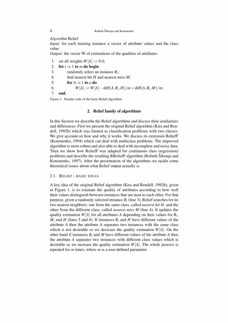
Algorithm ReliefInput: for each training instance a vector of attribute values and the classvalueOutput: the vector W of estimations of the qualities of attributes
1. set all weights W [A] := 0.0;2. for i := 1 to m do begin3. randomly select an instance Ri;4. find nearest hit H and nearest miss M;5. for A := 1 to a do6. W [A] := W [A]−diff(A,Ri,H)/m+diff(A,Ri,M)/m;7. end;
Figure 1. Pseudo code of the basic Relief algorithm
2. Relief family of algorithms
In this Section we describe the Relief algorithms and discuss their similaritiesand differences. First we present the original Relief algorithm (Kira and Ren-dell, 1992b) which was limited to classification problems with two classes.We give account on how and why it works. We discuss its extension ReliefF(Kononenko, 1994) which can deal with multiclass problems. The improvedalgorithm is more robust and also able to deal with incomplete and noisy data.Then we show how ReliefF was adapted for continuous class (regression)problems and describe the resulting RReliefF algorithm (Robnik Sikonja andKononenko, 1997). After the presentation of the algorithms we tackle sometheoretical issues about what Relief output actually is.
2.1. RELIEF - BASIC IDEAS
A key idea of the original Relief algorithm (Kira and Rendell, 1992b), givenin Figure 1, is to estimate the quality of attributes according to how welltheir values distinguish between instances that are near to each other. For thatpurpose, given a randomly selected instance Ri (line 3), Relief searches for itstwo nearest neighbors: one from the same class, called nearest hit H, and theother from the different class, called nearest miss M (line 4). It updates thequality estimation W [A] for all attributes A depending on their values for Ri,M, and H (lines 5 and 6). If instances Ri and H have different values of theattribute A then the attribute A separates two instances with the same classwhich is not desirable so we decrease the quality estimation W [A]. On theother hand if instances Ri and M have different values of the attribute A thenthe attribute A separates two instances with different class values which isdesirable so we increase the quality estimation W [A]. The whole process isrepeated for m times, where m is a user-defined parameter.

Theoretical and Empirical Analysis of ReliefF and RReliefF 5
Algorithm ReliefFInput: for each training instance a vector of attribute values and the classvalueOutput: the vector W of estimations of the qualities of attributes
1. set all weights W [A] := 0.0;2. for i := 1 to m do begin3. randomly select an instance Ri;4. find k nearest hits H j;5. for each class C 6= class(Ri) do6. from class C find k nearest misses M j(C);7. for A := 1 to a do
8. W [A] := W [A] -k∑j=1
diff(A,Ri,H j)/(m · k) +
9. ∑C 6=class(Ri)
[ P(C)1−P(class(Ri))
k∑j=1
diff(A,Ri,M j(C))]/(m · k);
10. end;Figure 2. Pseudo code of ReliefF algorithm
Function diff(A, I1, I2) calculates the difference between the values of theattribute A for two instances I1 and I2. For nominal attributes it was originallydefined as:
diff(A, I1, I2) ={
0 ;value(A, I1) = value(A, I2)1 ;otherwise (1)
and for numerical attributes as:
diff(A, I1, I2) =|value(A, I1)− value(A, I2)|
max(A)−min(A)(2)
The function diff is used also for calculating the distance between instancesto find the nearest neighbors. The total distance is simply the sum of distancesover all attributes (Manhattan distance).
The original Relief can deal with nominal and numerical attributes. How-ever, it cannot deal with incomplete data and is limited to two-class problems.Its extension, which solves these and other problems, is called ReliefF.
2.2. RELIEFF - EXTENSION
The ReliefF (Relief-F) algorithm (Kononenko, 1994) (see Figure 2) is notlimited to two class problems, is more robust and can deal with incompleteand noisy data. Similarly to Relief, ReliefF randomly selects an instance Ri(line 3), but then searches for k of its nearest neighbors from the same class,

6 Robnik Sikonja and Kononenko
called nearest hits H j (line 4), and also k nearest neighbors from each ofthe different classes, called nearest misses M j(C) (lines 5 and 6). It updatesthe quality estimation W [A] for all attributes A depending on their valuesfor Ri, hits H j and misses M j(C) (lines 7, 8 and 9). The update formula issimilar to that of Relief (lines 5 and 6 on Figure 1), except that we averagethe contribution of all the hits and all the misses. The contribution for eachclass of the misses is weighted with the prior probability of that class P(C)(estimated from the training set). Since we want the contributions of hits andmisses in each step to be in [0,1] and also symmetric (we explain reasonsfor that below) we have to ensure that misses’ probability weights sum to 1.As the class of hits is missing in the sum we have to divide each probabilityweight with factor 1−P(class(Ri)) (which represents the sum of probabilitiesfor the misses’ classes). The process is repeated for m times.
Selection of k hits and misses is the basic difference to Relief and ensuresgreater robustness of the algorithm concerning noise. User-defined parameterk controls the locality of the estimates. For most purposes it can be safely setto 10 (see (Kononenko, 1994) and discussion below).
To deal with incomplete data we change the diff function. Missing valuesof attributes are treated probabilistically. We calculate the probability that twogiven instances have different values for given attribute conditioned over classvalue:
− if one instance (e.g., I1) has unknown value:
diff(A, I1, I2) = 1−P(value(A, I2)|class(I1)) (3)
− if both instances have unknown value:
diff(A, I1, I2) = 1−#values(A)
∑V
(P(V |class(I1))×P(V |class(I2))
)(4)
Conditional probabilities are approximated with relative frequencies from thetraining set.
2.3. RRELIEFF - IN REGRESSION
We finish the description of the algorithmic family with RReliefF (Regres-sional ReliefF) (Robnik Sikonja and Kononenko, 1997). First we theoreticallyexplain what Relief algorithm actually computes.
Relief’s estimate W [A] of the quality of attribute A is an approximation ofthe following difference of probabilities (Kononenko, 1994):
W [A] = P(diff. value of A|nearest inst. from diff. class)− P(diff. value of A|nearest inst. from same class) (5)

Theoretical and Empirical Analysis of ReliefF and RReliefF 7
The positive updates of the weights (line 6 in Figure 1 and line 9 in Figure2) are actually forming the estimate of probability that the attribute discrim-inates between the instances with different class values, while the negativeupdates (line 6 in Figure 1 and line 8 in Figure 2) are forming the probabilitythat the attribute separates the instances with the same class value.
In regression problems the predicted value τ(·) is continuous, therefore(nearest) hits and misses cannot be used. To solve this difficulty, instead ofrequiring the exact knowledge of whether two instances belong to the sameclass or not, a kind of probability that the predicted values of two instancesare different is introduced. This probability can be modelled with the relativedistance between the predicted (class) values of two instances.
Still, to estimate W[A] in (5), information about the sign of each con-tributed term is missing (where do hits end and misses start). In the followingderivation Equation (5) is reformulated, so that it can be directly evaluatedusing the probability that predicted values of two instances are different. Ifwe rewrite
Pdi f f A = P(different value of A|nearest instances) (6)
Pdi f fC = P(different prediction|nearest instances) (7)
and
Pdi f fC|di f f A = P(diff. prediction|diff. value of A and nearest instances) (8)
we obtain from (5) using Bayes’ rule:
W [A] =Pdi f fC|di f f APdi f f A
Pdi f fC− (1−Pdi f fC|di f f A)Pdi f f A
1−Pdi f fC(9)
Therefore, we can estimate W [A] by approximating terms defined by Equa-tions 6, 7 and 8. This can be done by the algorithm on Figure 3.
Similarly to ReliefF we select random instance Ri (line 3) and its k nearestinstances I j (line 4). The weights for different prediction value τ(·) (line 6),different attribute (line 8), and different prediction & different attribute (line9 and 10) are collected in NdC, NdA[A], and NdC&dA[A], respectively. The finalestimation of each attribute W [A] (Equation (9)) is computed in lines 14 and15.
The term d(i, j) in Figure 3 (lines 6, 8 and 10) takes into account thedistance between the two instances Ri and I j. Rationale is that closer instancesshould have greater influence, so we exponentially decrease the influence ofthe instance I j with the distance from the given instance Ri:
d(i, j) =d1(i, j)
∑kl=1 d1(i, l)
and (10)

8 Robnik Sikonja and Kononenko
Algorithm RReliefFInput: for each training instance a vector of attribute values x and predictedvalue τ(x)Output: vector W of estimations of the qualities of attributes
1. set all NdC, NdA[A], NdC&dA[A], W [A] to 0;2. for i := 1 to m do begin3. randomly select instance Ri;4. select k instances I j nearest to Ri;5. for j := 1 to k do begin6. NdC := NdC +diff(τ(·),Ri, I j) ·d(i, j);7. for A := 1 to a do begin8. NdA[A] := NdA[A]+diff(A,Ri, I j) ·d(i, j);9. NdC&dA[A] := NdC&dA[A]+diff(τ(·),Ri, I j)·
10. diff(A,Ri, I j) ·d(i, j);11. end;12. end;13. end;14. for A := 1 to a do15. W [A] := NdC&dA[A]/NdC - (NdA[A]−NdC&dA[A])/(m−NdC);Figure 3. Pseudo code of RReliefF algorithm
d1(i, j) = e−
(rank(Ri,I j)
σ
)2
(11)
where rank(Ri, I j) is the rank of the instance I j in a sequence of instancesordered by the distance from Ri and σ is a user defined parameter controllingthe influence of the distance. Since we want to stick to the probabilistic in-terpretation of the results we normalize the contribution of each of k nearestinstances by dividing it with the sum of all k contributions. The reason forusing ranks instead of actual distances is that actual distances are problemdependent while by using ranks we assure that the nearest (and subsequent aswell) instance always has the same impact on the weights.
ReliefF was using a constant influence of all k nearest instances I j fromthe instance Ri. For this we should define d1(i, j) = 1/k.
Discussion about different distance functions can be found in followingsections.
2.4. COMPUTATIONAL COMPLEXITY
For n training instances and a attributes Relief (Figure 1) makes O(m · n ·a) operations. The most complex operation is selection of the nearest hit

Theoretical and Empirical Analysis of ReliefF and RReliefF 9
and miss as we have to compute the distances between R and all the otherinstances which takes O(n ·a) comparisons.
Although ReliefF (Figure 2) and RReliefF (Figure 3) look more compli-cated their asymptotical complexity is the same as that of original Relief,i.e., O(m · n · a). The most complex operation within the main for loop isselection of k nearest instances. For it we have to compute distances fromall the instances to R, which can be done in O(n · a) steps for n instances.This is the most complex operation, since O(n) is needed to build a heap,from which k nearest instances are extracted in O(k logn) steps, but this isless than O(n ·a).
Data structure k-d (k-dimensional) tree (Bentley, 1975; Sefgewick, 1990)is a generalization of the binary search tree, which instead of one key uses kkeys (dimensions). The root of the tree contains all the instances. Each inte-rior node has two successors and splits instances recursively into two groupsaccording to one of k dimensions. The recursive splitting stops when there areless than a predefined number of instances in a node. For n instances we canbuild the tree where split on each dimension maximizes the variance in thatdimension and instances are divided into groups of approximately the samesize in time proportional to O(k · n · logn). With such tree called optimizedk-d tree we can find t nearest instances to the given instance in O(logn) steps(Friedman et al., 1975).
If we use k-d tree to implement the search for nearest instances we can re-duce the complexity of all three algorithms to O(a ·n · logn) (Robnik Sikonja,1998). For Relief we first build the optimized k-d tree (outside the main loop)in O(a · n · logn) steps so we need only O(m · a) steps in the loop and thetotal complexity of the algorithm is now the complexity of the preprocessingwhich is O(a ·n · logn). The required sample size m is related to the problemcomplexity (and not to the number of instances) and is typically much morethan logn so asymptotically we have reduced the complexity of the algorithm.Also it does not make sense to use sample size m larger than the number ofinstances n.
The computational complexity of ReliefF and RReliefF using k-d trees isthe same as that of Relief. They need O(a ·n · logn) steps to build k-d tree, andin the main loop they select t nearest neighbors in logn steps, update weightsin O(t ·a) but O(m(t ·a+ logn)) is asymptotically less than the preprocessingwhich means that the complexity has reduced to O(a · n · logn). This analy-sis shows that ReliefF family of algorithms is actually in the same order ofcomplexity as multikey sort algorithms.
Several authors have observed that the use of k-d trees becomes ineffi-cient with increasing number of attributes (Friedman et al., 1975; Deng andMoore, 1995; Moore et al., 1997) and this was confirmed for Relief family ofalgorithms as well (Robnik Sikonja, 1998).

10 Robnik Sikonja and Kononenko
Kira and Rendell (Kira and Rendell, 1992b) consider m an arbitrary chosenconstant and claim that the complexity of Relief is O(a ·n). If we accept theirargument than the complexity of ReliefF and RReliefF is also O(a · n), andthe above analysis using k-d trees is useless. However, if we want to obtainsensible and reliable results with Relief algorithms then the required samplesize m is related to the problem complexity and is not constant as we willshow below.
2.5. GENERAL FRAMEWORK OF RELIEF ALGORITHMS
By rewriting Equation (5) into a form suitable also for regression
W [A] = P(diff. value of A|near inst. with diff. prediction)− P(diff. value of A|near inst. with same prediction) (12)
we see that we are actually dealing with (dis)similarities of attributes andprediction values (of near instances). A generalization of Relief algorithmswould take into account the similarity of the predictions τ and of the attributesA and combine them into a generalized weight:
WG[A] = ∑I1,I2∈I
similarity(τ, I1, I2) · similarity(A, I1, I2) (13)
where I1 and I2 were appropriate samples drawn from the instance populationI . If we use [0,1] normalized similarity function (like e.g., diff) than withthese weights we can model the following probabilities:
• P(similar A|similar τ), P(dissimilar A|similar τ), and
• P(similar A|dissimilar τ), P(dissimilar A|dissimilar τ).
In the probabilistic framework we can write:
P(similar A|similar τ)+P(dissimilar A|similar τ) = 1 (14)P(similar A|dissimilar τ)+P(dissimilar A|dissimilar τ) = 1 (15)
so it is sufficient to compute one of the pair of probabilities from above andstill to get all the information.
Let us think for a moment what we intuitively expect from a good attributeestimator. In our opinion good attributes separate instances with differentprediction values and do not separate instances with close prediction values.These considerations are fulfilled by taking one term from each group ofprobabilities from above and combine them in a sensible way. If we rewriteRelief’s weight from Equation (12):
W [A] = 1−P(similar A|dissimilar τ)−1+P(similar A|similar τ)
Theoretical and Empirical Analysis of ReliefF and RReliefF 11
= P(similar A|similar τ)−P(similar A|dissimilar τ)
we see that this is actually what Relief algorithms do: they reward attributefor not separating similar prediction values and punish it for not separatingdifferent prediction values.
The similarity function used by Relief algorithms is
similarity(A, I1, I2) =−diff(A, I1, I2)
which enables intuitive probability based interpretation of results. We couldget variations of Relief estimator by taking different similarity functions andby combining the computed probabilities in a different way. For example,the Contextual Merit (CM) algorithm (Hong, 1997) uses only the instanceswith different prediction values and therefore it takes only the first term ofEquation (12) into account. As a result CM only rewards attribute if it sep-arates different prediction values and ignores additional information, whichthe similar prediction values offer. Consequently CM is less sensitive thanRelief algorithms are, e.g., in parity problems with three important attributesCM separates important from unimportant attributes for a factor of 2 to 5 andonly 1.05-1.19 with numerical attributes while with ReliefF under the sameconditions this factor is over 100. Part of troubles CM has with numericalattributes also comes from the fact that it does not take the second term intoaccount, namely it does not punish attributes for separating similar predictionvalues. As numerical attributes are very likely to do that CM has to use othertechniques to confront this effect.
2.6. RELIEF AND IMPURITY FUNCTIONS
Estimations of Relief algorithms are strongly related to impurity functions(Kononenko, 1994). When the number of nearest neighbors increases i.e.,when we eliminate the requirement that the selected instance is the nearest,Equation (5) becomes
W ′[A] = P(different value of A|different class)− P(different value of A|same class) (16)
If we rewritePeqval = P(equal value of A)
Psamecl = P(same class)
Psamecl|eqval = P(same class|equal value of A)
we obtain using Bayes’ rule:
W ′[A] =Psamecl|eqvalPeqval
Psamecl− (1−Psamecl|eqval)Peqval
1−Psamecl
12 Robnik Sikonja and Kononenko
For sampling with replacement in strict sense the following equalitieshold:
Psamecl = ∑C
P(C)2
Psamecl|eqval = ∑V
(P(V )2
∑V P(V )2 ×∑C
P(C|V )2
)
Using the above equalities we obtain:
W ′[A] =Peqval ×Ginigain′(A)Psamecl(1−Psamecl)
(17)
where
Ginigain′(A) = ∑V
(P(V )2
∑V P(V )2 ×∑C
P(C|V )2
)−∑
CP(C)2 (18)
is highly correlated with the Gini-index gain (Breiman et al., 1984) for classesC and values V of attribute A. The difference is that instead of factor
P(V )2
∑V P(V )2
the Gini-index gain usesP(V )
∑V P(V )= P(V )
Equation (17) (which we call myopic ReliefF), shows strong correlation ofRelief’s weights with the Gini-index gain. The probability Pequal = ∑V P(V )2
that two instances have the same value of attribute A in Equation (17) is a kindof normalization factor for multi-valued attributes. Impurity functions tend tooverestimate multi-valued attributes and various normalization heuristics areneeded to avoid this tendency (e.g., gain ratio (Quinlan, 1986), distance mea-sure (Mantaras, 1989), and binarization of attributes (Cestnik et al., 1987)).Equation (17) shows that Relief exhibits an implicit normalization effect.Another deficiency of Gini-index gain is that its values tend to decrease withthe increasing number of classes. Denominator, which is constant factor inEquation (17) for a given attribute, again serves as a kind of normalizationand therefore Relief’s estimates do not exhibit such strange behavior as Gini-index gain does. This normalization effect remains even if Equation (17) isused as (myopic) attribute estimator. The detailed bias analysis of variousattribute estimation algorithms including Gini-index gain and myopic ReliefFcan be found in (Kononenko, 1995).
The above derivation eliminated from the probabilities the condition thatthe instances are the nearest. If we put it back we can interpret Relief’s es-timates as the average over local estimates in smaller parts of the instance

Theoretical and Empirical Analysis of ReliefF and RReliefF 13
space. This enables Relief to take into account the context of other attributes,i.e. the conditional dependencies between the attributes given the predictedvalue, which can be detected in the context of locality. From the global pointof view, these dependencies are hidden due to the effect of averaging overall training instances, and exactly this makes the impurity functions myopic.The impurity functions use correlation between the attribute and the classdisregarding the context of other attributes. This is the same as using theglobal point of view and disregarding local peculiarities. The power of Reliefis its ability to exploit information locally, taking the context into account,but still to provide the global view.
-0.1
0
0.1
0.2
0.3
0.4
0.5
0 10 20 30 40 50 60 70 80 90
Number of nearest neighbors
Rel
iefF
's e
stim
ate
Informative
Random
Figure 4. ReliefF’s estimates of informative attribute are deteriorating with increasing numberof nearest neighbors in parity domain.
We illustrate this in Figure 4 which shows dependency of ReliefF’s esti-mate to the number of nearest neighbors taken into account. The estimatesare for the parity problem with two informative, 10 random attributes, and200 examples. The dotted line shows how the ReliefF’s estimate of one ofinformative attributes is becoming more and more myopic with the increasingnumber of the nearest neighbors and how the informative attribute eventuallybecomes indistinguishable from the unimportant attributes. The negative esti-mate of random attributes with small numbers of neighbors is a consequenceof slight asymmetry between hits and misses. Recall that Relief algorithm(Figure 1) randomly selects an instance R and its nearest instance from thesame class H and from different class M. Random attributes with differentvalues at R and H get negative update. Random attributes with different valuesat R and M get positive update. With larger number of nearest neighbors thepositive and negative updates are equiprobable and the quality estimates ofrandom attributes is zero. The miss has different class value therefore therehas to be at least some difference also in the values of the important attributes.The sum of the differences in the values of attributes forms the distance, there-fore if there is a difference in the values of the important attribute and also inthe values of some random attributes, such instances are less likely to be in the

14 Robnik Sikonja and Kononenko
nearest neighborhood. This is especially so when we are considering only asmall number of nearest instances. The positive update of random attributes istherefore less likely than the negative update and the total sum of all updatesis slightly negative.
2.7. RELIEF’S WEIGHTS AS THE PORTION OF EXPLAINED CONCEPTCHANGES
We analyze the behavior of Relief when the number of the examples ap-proaches infinity i.e., when the problem space is densely covered with theexamples. We present the necessary definitions and prove that Relief’s qualityestimates can be interpreted as the ratio between the number of the explainedchanges in the concept and the number of examined instances. The exact formof this property differs between Relief, ReliefF and RReliefF.
We start with Relief and claim that in a classification problem as the num-ber of examples goes to infinity Relief’s weights for each attribute convergeto the ratio between the number of class label changes the attribute is re-sponsible for and the number of examined instances. If a certain change canbe explained in several different ways, all the ways share the credit for itin the quality estimate. If several attributes are involved in one way of theexplanation all of them get the credit in their quality estimate. We formallypresent the definitions and the property.
DEFINITION 2.1. Let B(I) be the set of instances from I nearest to theinstance I ∈I which have different prediction value τ than I:
B(I) = {Y ∈I ;diff(τ, I,Y ) > 0∧Y = arg minY∈I
δ (I,Y )} (19)
Let b(I) be a single instance from the set B(I) and p(b(I)) a probability thatit is randomly chosen from B(I). Let A(I,b(I)) be a set of attributes withdifferent values at instances I and b(I).
A(I,b(I)) = {A ∈A ; b(I) ∈ B(I)∧diff(A, I,b(I)) > 0} (20)
We say that attributes A ∈ A(I,b(I)) are responsible for the change of thepredicted value of the instance I to the predicted value of b(I) as the changeof their values is one of the minimal number of changes required for changingthe predicted value of I to b(I). If the sets A(I,b(I)) are different we say thatthere are different ways to explain the changes of the predicted value of Ito the predicted value b(I). The probability of certain way is equal to theprobability that b(I) is selected from B(I).
Let A(I) be a union of sets A(I,b(I)):
A(I) =⋃
b(I)∈B(I)
A(I,b(I)) (21)
Theoretical and Empirical Analysis of ReliefF and RReliefF 15
We say that the attributes A ∈ A(I) are responsible for the change of thepredicted value of the instance I as the change of their values is the minimalnecessary change of the attributes’ values of I required to change its predictedvalue. Let the quantity of this responsibility take into account the change ofthe predicted value and the change of the attribute:
rA(I,b(I)) = p(b(I)) ·diff(τ, I,b(I)) ·diff(A, I,b(I)) (22)
The ratio between the responsibility of the attribute A for the predicted valuesof the set of cases S and the cardinality m of that set is therefore:
RA =1m ∑
I∈S
rA(I,b(I)) (23)
PROPERTY 2.1. Let the concept be described with the attributes A ∈ Aand n noiseless instances I ∈I ; let S ⊆I be the set of randomly selectedinstances used by Relief (line 3 on Figure 1) and let m be the cardinalityof that set. If Relief randomly selects the nearest instances from all possiblenearest instances then for its quality estimate W [A] the following propertyholds:
limn→∞
W [A] = RA (24)
The quality estimate of the attribute can therefore be explained as the ratio ofthe predicted value changes the attribute is responsible for to the number ofthe examined instances.
Proof. Equation (24) can be explained if we look into the spatial represen-tation. There are a number of different characteristic regions of the problemspace which we usually call peaks. The Relief algorithms selects an instanceR from S and compares the value of the attribute and the predicted value ofits nearest instances selected from the set I (line 6 on Figure 1), and thanupdates the quality estimates according to these values. For Relief this mean:W [A] := W [A] + diff(A,R,M)/m− diff(A,R,H)/m, where M is the nearestinstance from the different class and H is the nearest instance from the sameclass.
When the number of the examples is sufficient (n→ ∞), H must be fromthe same characteristic region as R and its values of the attributes convergeto the values of the instance R. The contribution of the term −diff(A,R,H) toW [A] in the limit is therefore 0.
Only terms diff(A,R,M) contribute to W [A]. The instance M is randomlyselected nearest instance with different prediction than R, therefore in noise-less problems there must be at least some difference in the values of theattributes and M is therefore an instance of b(R) selected with probabilityp(M). As M has different prediction value than R the value diff(τ,R,M) = 1.

16 Robnik Sikonja and Kononenko
The attributes with different values at R and M constitute the set A(R,M).The contribution of M to W [A] for the attributes from the A(R,M) equalsdiff(A,R,M)/m = diff(τ,R,M)) ·diff(A,R,M))/m with probability p(M)).
Relief selects m instances I ∈S and for each I randomly selects its nearestmiss b(I) with probability p(b(I)). The sum of updates of W [A] for each at-tribute is therefore: ∑I∈S p(b(I))diff(τ,R,b(I))diff(A,R,b(I))/m) = RA, andthis concludes the proof.
Let us show an example, which illustrates the idea. We have a Booleanproblem where the class value is defined as τ = (A1∧A2)∨ (A1∧A3). TableI gives a tabular description of the problem. The right most column showswhich of the attributes is responsible for the change of the predicted value.
Table I. Tabular description of the concept τ = (A1∧A2)∨ (A1∧A3) and the responsibility ofthe attributes for the change of the predicted value.
line A1 A2 A3 τ responsible attributes1 1 1 1 1 A12 1 1 0 1 A1 or A23 1 0 1 1 A1 or A34 1 0 0 0 A2 or A35 0 1 1 0 A16 0 1 0 0 A17 0 0 1 0 A18 0 0 0 0 (A1, A2) or (A1, A3)
In line 1 we say that A1 is responsible for the class assignment becausechanging its value to 0 would change τ to 0, while changing only one of A2 orA3 would leave τ unchanged. In line 2 changing any of A1 or A2 would changeτ too, so A1 and A2 represent two manners how to change τ and also share theresponsibility. Similarly we explain lines 3 to 7, while in line 8 changing onlyone attribute is not enough for τ to change. However, changing A1 and A2 orA1 and A3 changes τ . Therefore the minimal number of required changes is2 and the credit (and updates in the algorithm) goes to both A1 and A2 or A1and A3. There are 8 peaks in this problem which are equiprobable so A1 gets
the estimate 4+2· 12 +2· 1
28 = 3
4 = 0.75 (it is alone responsible for lines 1, 5, 6,and 7, shares the credit for lines 2 and 3 and cooperates in both credits for
line 8). A2 (and similarly A3) gets estimate 2· 12 + 1
28 = 3
16 = 0.1875 (it shares theresponsibility for lines 2 and 4 and cooperates in one half of line 8).
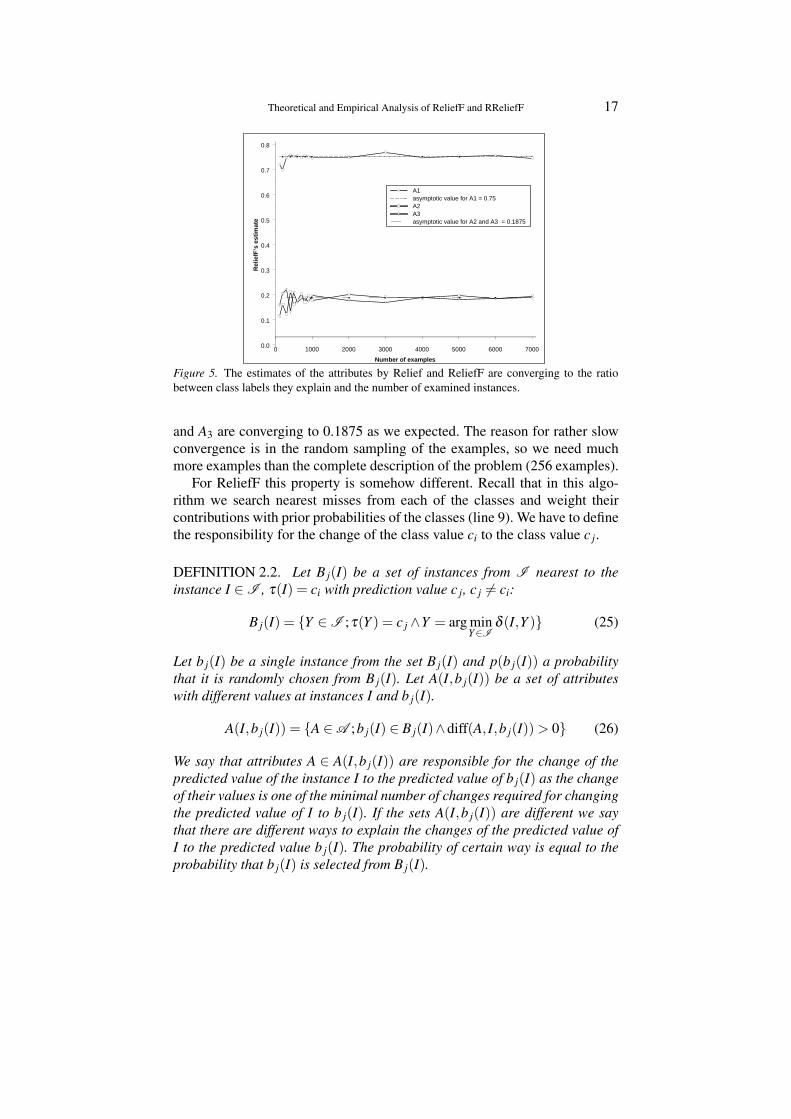
Figure 5 shows the estimates of the quality of the attributes for this prob-lem for Relief (and also ReliefF). As we wanted to scatter the concept weadded besides three important attributes also five random binary attributes tothe problem description. We can observe that as we increase the number of theexamples the estimate for A1 is converging to 0.75, while the estimates for A2
Theoretical and Empirical Analysis of ReliefF and RReliefF 17
0 1000 2000 3000 4000 5000 6000 7000
Number of examples
0.0
0.1
0.2
0.3
0.4
0.5
0.6
0.7
0.8
Rel
iefF
’s e
stim
ate
A1asymptotic value for A1 = 0.75A2A3asymptotic value for A2 and A3 = 0.1875
Figure 5. The estimates of the attributes by Relief and ReliefF are converging to the ratiobetween class labels they explain and the number of examined instances.
and A3 are converging to 0.1875 as we expected. The reason for rather slowconvergence is in the random sampling of the examples, so we need muchmore examples than the complete description of the problem (256 examples).
For ReliefF this property is somehow different. Recall that in this algo-rithm we search nearest misses from each of the classes and weight theircontributions with prior probabilities of the classes (line 9). We have to definethe responsibility for the change of the class value ci to the class value c j.
DEFINITION 2.2. Let B j(I) be a set of instances from I nearest to theinstance I ∈I , τ(I) = ci with prediction value c j, c j 6= ci:
B j(I) = {Y ∈I ;τ(Y ) = c j ∧Y = arg minY∈I
δ (I,Y )} (25)
Let b j(I) be a single instance from the set B j(I) and p(b j(I)) a probabilitythat it is randomly chosen from B j(I). Let A(I,b j(I)) be a set of attributeswith different values at instances I and b j(I).
A(I,b j(I)) = {A ∈A ;b j(I) ∈ B j(I)∧diff(A, I,b j(I)) > 0} (26)
We say that attributes A ∈ A(I,b j(I)) are responsible for the change of thepredicted value of the instance I to the predicted value of b j(I) as the changeof their values is one of the minimal number of changes required for changingthe predicted value of I to b j(I). If the sets A(I,b j(I)) are different we saythat there are different ways to explain the changes of the predicted value ofI to the predicted value b j(I). The probability of certain way is equal to theprobability that b j(I) is selected from B j(I).

18 Robnik Sikonja and Kononenko
Let A j(I) be a union of sets A(I,b j(I)):
A j(I) =⋃
b j(I)∈B j(I)
A(I,b j(I)) (27)
We say that the attributes A ∈ A j(I) are responsible for the change of pre-dicted value ci of the instance I to the value c j 6= ci as the change of theirvalues is the minimal necessary change of the attributes’ values of I requiredto change its predicted value to c j. Let the quantity of this responsibility takeinto account the change of the predicted value and the change of the attribute:
rA j(I,b(I)) = p(b j(I)) ·diff(τ , I,b j(I)) ·diff(A, I,b j(I)) (28)
The ratio between the responsibility of the attribute A for the change of pre-dicted values from ci to c j for the set of cases S and the cardinality m of thatset is thus:
RA(i, j) =1m ∑
I∈S
rA j(I,b j(I)) (29)
PROPERTY 2.2. Let p(ci) represent the prior probability of the class ci.Under the conditions of Property 2.1, algorithm ReliefF behaves as:
limn→∞
W [A] =c
∑i=1
c
∑j=1j 6=i
p(ci)p(c j)1− p(ci)
RA(i, j) (30)
We can therefore explain the quality estimates as the ratio of class valueschanges the attribute is responsible for to the number of the examined in-stances weighted with the prior probabilities of class values.
Proof is similar to the proof of Property 2.1. Algorithm ReliefF selects aninstance R∈S (line 3 on Figure 2). Probability of R being labelled with classvalue ci is equal to prior probability of that value p(ci). The algorithm thansearches for k nearest instances from the same class and k nearest instancesfrom each of the other classes (line 6 on Figure 2) and and than updates thequality estimates W [A] according to these values (lines 8 and 9 on Figure 2).
As the number of the examples is sufficient (n → ∞), instances H j mustbe from the same characteristic region as R and their values of the attributesconverge to the values of the attributes of the instance R. The contribution ofnearest hits to W [A] in the limit is therefore 0.
Only nearest misses contribute to W [A]. The instances M j are randomlyselected nearest instances with different prediction than R, therefore in thenoiseless problems there must be at least some difference in the values of theattributes and all M j are therefore instances of b j(R) selected with probabilityp j(M). The contributions of k instances are weighted with the probabilitiesp(b j(R)).

Theoretical and Empirical Analysis of ReliefF and RReliefF 19
As M j have different prediction value than R the value diff(τ ,R,M j) = 1.The attributes with different values at R and M j constitute the set A j(R,b j(R)).The contribution of the instances M j to W [A] for the attributes from theA j(R,b j(R)) equals ∑c
j=1j 6=i
p(c j)1−p(ci)
p(b j(R))diff(A,Ri,b j(R))/m.
ReliefF selects m instances I ∈S where p(ci) ·m of them are labelled withci. For each I it randomly selects its nearest misses b j(I), j 6= i with probabil-ities p(b j(I)). The sum of updates of W [A] for each attribute is therefore:
W [A] = ∑I∈S
c
∑j=1j 6=i
p(c j)1− p(ci)
p(b j(I))diff(C, I,b j(I))diff(A, I,b j(I))/m
= ∑I∈S
c
∑j=1j 6=i
p(c j)1− p(ci)
rA j(I,b(I))/m,
This can be rewritten as the sum over the class values as only the instanceswith class value ci contribute to the RA(i, j):
=c
∑i=1
p(ci)c
∑j=1j 6=i
p(c j)1− p(ci)
RA(i, j)
=c
∑i=1
c
∑j=1j 6=i
p(ci)p(c j)1− p(ci)
RA(i, j),
which we wanted to prove.
COROLLARY 2.3. In two class problems where diff function is symmetric:diff(A, I1, I2) = diff(A, I2, I1) Property 2.2 is equivalent to Property 2.1.
Proof. As diff is symmetric also the responsibility is symmetric RA(i, j) =RA( j, i). Let us rewrite Equation (30) with p(c1) = p and p(c2) = 1− p.By taking into account that we are dealing with only two classes we getlimn→∞W [A] = RA(1,2) = RA.
In a Boolean noiseless case as in the example presented above the fastestconvergence would be with only 1 nearest neighbor. With more nearest neigh-bors (default with the algorithms ReliefF and RReliefF) we need more ex-amples to see this effect as all of them has to be from the same/nearestpeak.
The interpretation of the quality estimates with the ratio of the explainedchanges in the concept is true for RReliefF as well, as it also computes Equa-tion (12), however, the updates are proportional to the size of the differencein the prediction value. The exact formulation and proof remain for furtherwork.

20 Robnik Sikonja and Kononenko
Note that the sum of the expressions (24) and (30) for all attributes isusually greater than 1. In certain peaks there are more than one attributeresponsible for the class assignment i.e., the minimal number of attributechanges required for changing the value of the class is greater than 1 (e.g.,line 8 in Table I). The total number of the explanations is therefore greater(or equal) than the number of the inspected instances. As Relief algorithmsnormalize the weights with the number of the inspected instances m and notthe total number of possible explanations, the quality estimations are not pro-portional to the attributes’s responsibility but present rather a portion of theexplained changes. For the estimates to represent the proportions we wouldhave to change the algorithm and thereby lose the probabilistic interpretationof attributes’ weights.
When we omit the assumption of the sufficient number of the examplesthen the estimates of the attributes can be greater than their asymptotic val-ues because the instances more distant than the minimal number of requiredchanges might be selected into the set of nearest instances and the attributesmight be positively updated also when they are responsible for the changeswhich are more distant than the minimal number of required changes.
The behavior of the Relief algorithm in the limit (Equation (2.1)) is thesame as the the asymptotic behavior of the algorithm Contextual Merit (CM)(Hong, 1997) which uses only the contribution of nearest misses. In multiclass problems CM searches for nearest instances from different class disre-garding the actual class they belong, while ReliefF selects equal number ofinstances from each of the different classes and normalizes their contributionwith their prior probabilities. The idea is that the algorithm should estimatethe ability of attributes to separate each pair of the classes regardless of whichtwo classes are closest to each other. It was shown (Kononenko, 1994) thatthis approach is superior and the same normalization factors occur also inasymptotic behavior of ReliefF given by Equation (2.2).
Based solely on the asymptotic properties one could come to, in our opin-ion, the wrong conclusion that it is sufficient for estimation algorithms toconsider only nearest instances with different prediction value. While thenearest instances with the same prediction have no effect when the num-ber of the instances is unlimited they nevertheless play an important role inproblems of practical sizes.
Clearly the interpretation of Relief’s weights as the ratio of explained con-cept changes is more comprehensible than the interpretation with the dif-ference of two probabilities. The responsibility for the explained changes ofthe predicted value is intuitively clear. Equation 24 is non probabilistic, un-conditional, and contains a simple ratio, which can be understood taking theunlimited number of the examples into account. The actual quality estimates
Theoretical and Empirical Analysis of ReliefF and RReliefF 21
of the attributes in given problem are therefore approximations of these idealestimates which occur only with abundance of data.
3. Parameters of ReliefF and RReliefF
In this section we address different parameters of ReliefF and RReliefF: theimpact of different distance measures, the use of numerical attributes, howdistance can be taken into account, the number of nearest neighbors used andthe number of iterations.
The datasets not defined in the text and used in our demonstrations andtests are briefly described in the Appendix.
3.1. METRICS
The diff(Ai, I1, I2) function calculates the difference between the values of theattribute Ai for two instances I1 and I2. Sum of differences over all attributes isused to determine the distance between two instances in the nearest neighborscalculation.
δ (I1, I2) =a
∑i=1
diff(Ai, I2, I2) (31)
This looks quite simple and parameterless, however, in instance based learn-ing there are a number of feature weighting schemes which assign differentweights to the attributes in the total sum:
δ (I1, I2) =a
∑i=1
w(Ai)diff(Ai, I1, I2) (32)
ReliefF’s estimates of attributes’ quality can be successfully used as suchweights (Wettschereck et al., 1997).
Another possibility is to form a metric in a different way:
δ (I1, I2) = (a
∑i=1
diff(Ai, I2, I2)p)1p (33)
which for p = 1 gives Manhattan distance and for p = 2 Euclidean distance.In our use of Relief algorithms we never noticed any significant difference inthe estimations using these two metrics. For example, on the regression prob-lems from the UCI repository (Murphy and Aha, 1995) (8 tasks: Abalone,Auto-mpg, Autoprice, CPU, Housing, PWlinear, Servo, and Wisconsin breastcancer) the average (linear) correlation coefficient is 0.998 and (Spearman’s)rank correlation coefficient is 0.990.
22 Robnik Sikonja and Kononenko
3.2. NUMERICAL ATTRIBUTES
If we use diff function as defined by (1) and (2) we run into the problemof underestimating numerical attributes. Let us illustrate this by taking twoinstances with 2 and 5 being their values of attribute Ai, respectively. If Ai isthe nominal attribute, the value of diff(Ai,2,5) = 1, since the two categoricalvalues are different. If Ai is the numerical attribute, diff(Ai,2,5) = |2−5|
7 ≈0.43. Relief algorithms use results of diff function to update their weightstherefore with this form of diff numerical attributes are underestimated.
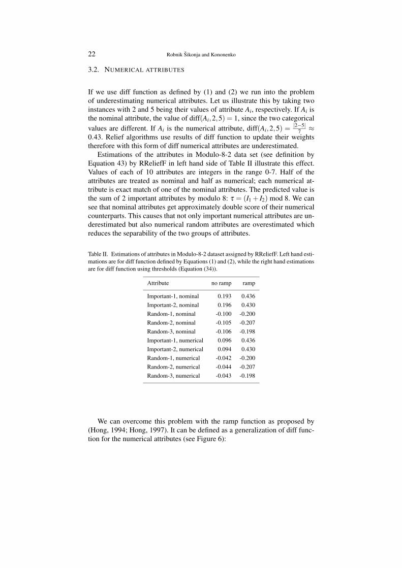
Estimations of the attributes in Modulo-8-2 data set (see definition byEquation 43) by RReliefF in left hand side of Table II illustrate this effect.Values of each of 10 attributes are integers in the range 0-7. Half of theattributes are treated as nominal and half as numerical; each numerical at-tribute is exact match of one of the nominal attributes. The predicted value isthe sum of 2 important attributes by modulo 8: τ = (I1 + I2) mod 8. We cansee that nominal attributes get approximately double score of their numericalcounterparts. This causes that not only important numerical attributes are un-derestimated but also numerical random attributes are overestimated whichreduces the separability of the two groups of attributes.
Table II. Estimations of attributes in Modulo-8-2 dataset assigned by RReliefF. Left hand esti-mations are for diff function defined by Equations (1) and (2), while the right hand estimationsare for diff function using thresholds (Equation (34)).
Attribute no ramp ramp
Important-1, nominal 0.193 0.436Important-2, nominal 0.196 0.430Random-1, nominal -0.100 -0.200Random-2, nominal -0.105 -0.207Random-3, nominal -0.106 -0.198Important-1, numerical 0.096 0.436Important-2, numerical 0.094 0.430Random-1, numerical -0.042 -0.200Random-2, numerical -0.044 -0.207Random-3, numerical -0.043 -0.198
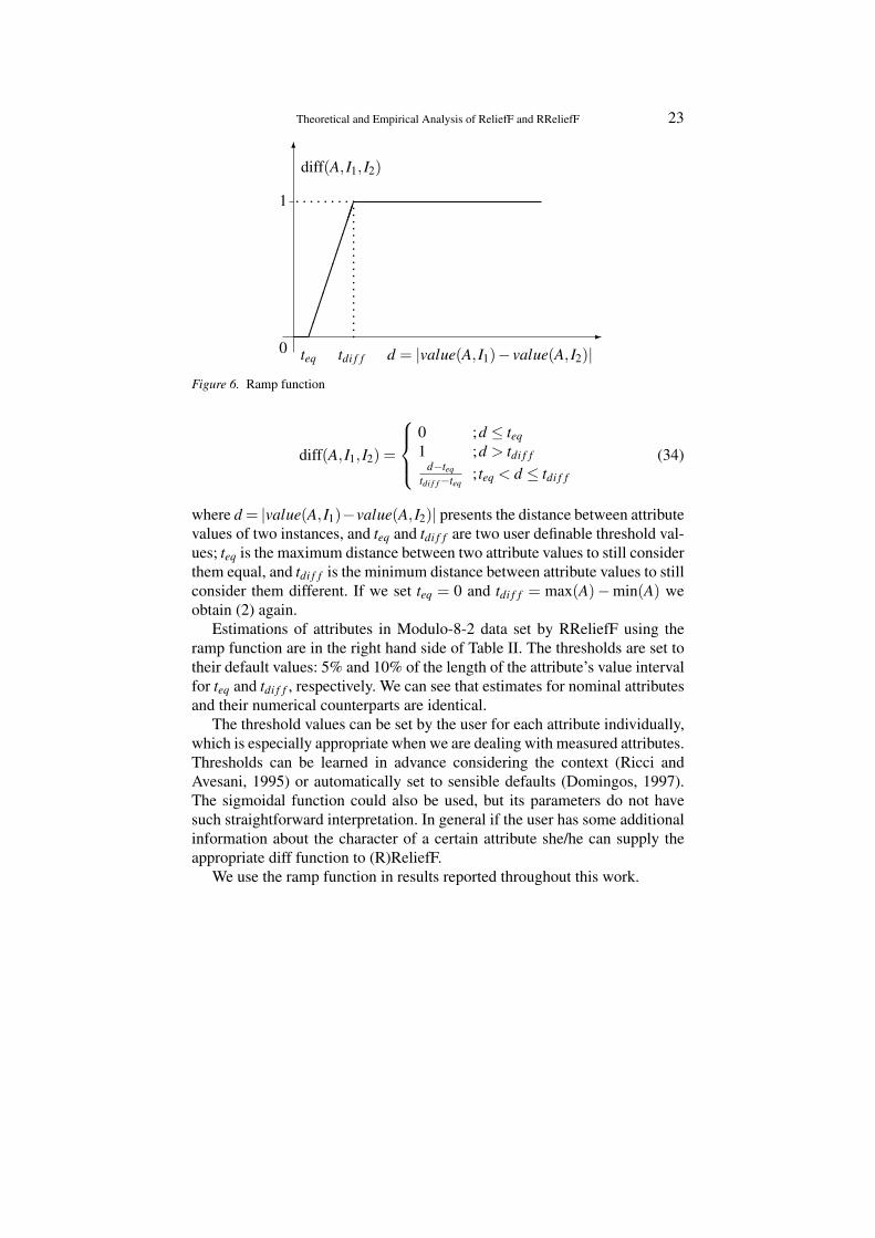
We can overcome this problem with the ramp function as proposed by(Hong, 1994; Hong, 1997). It can be defined as a generalization of diff func-tion for the numerical attributes (see Figure 6):
Theoretical and Empirical Analysis of ReliefF and RReliefF 23
0
1
teq tdi f f d = |value(A, I1)− value(A, I2)|££££££££££.....................
.........
6
-
diff(A, I1, I2)
Figure 6. Ramp function
diff(A, I1, I2) =
0 ;d ≤ teq1 ;d > tdi f f
d−teqtdi f f−teq
; teq < d ≤ tdi f f
(34)
where d = |value(A, I1)−value(A, I2)| presents the distance between attributevalues of two instances, and teq and tdi f f are two user definable threshold val-ues; teq is the maximum distance between two attribute values to still considerthem equal, and tdi f f is the minimum distance between attribute values to stillconsider them different. If we set teq = 0 and tdi f f = max(A)−min(A) weobtain (2) again.
Estimations of attributes in Modulo-8-2 data set by RReliefF using theramp function are in the right hand side of Table II. The thresholds are set totheir default values: 5% and 10% of the length of the attribute’s value intervalfor teq and tdi f f , respectively. We can see that estimates for nominal attributesand their numerical counterparts are identical.
The threshold values can be set by the user for each attribute individually,which is especially appropriate when we are dealing with measured attributes.Thresholds can be learned in advance considering the context (Ricci andAvesani, 1995) or automatically set to sensible defaults (Domingos, 1997).The sigmoidal function could also be used, but its parameters do not havesuch straightforward interpretation. In general if the user has some additionalinformation about the character of a certain attribute she/he can supply theappropriate diff function to (R)ReliefF.
We use the ramp function in results reported throughout this work.
24 Robnik Sikonja and Kononenko
3.3. TAKING DISTANCE INTO ACCOUNT
In instance based learning it is often considered useful to give more impactto the near instances than to the far ones i.e., to weight their impact inverselyproportional to their distance from the query point.
RReliefF is already taking the distance into account through Equations(10) and (11). By default we are using 70 nearest neighbors and exponen-tially decrease their influence with increasing distance from the query point.ReliefF originally used constant influence of k nearest neighbors with k setto some small number (usually 10). We believe that the former approach isless risky (as it turned out in a real world application (Dalaka et al., 2000))because as we are taking more near neighbors we reduce the risk of thefollowing pathological case: we have a large number of instances and a mixof nominal and numerical attributes where numerical attributes prevail; it ispossible that all the nearest neighbors are closer than 1 so that there are nonearest neighbors with differences in values of a certain nominal attribute. Ifthis happens in a large part of the problem space this attribute gets zero weight(or at least small and unreliable one). By taking more nearest neighbors withappropriately weighted influence we eliminate this problem.
ReliefF can be adjusted to take distance into account by changing the wayit updates it weights (lines 8 and 9 in Figure 2):
W [A] := W [A]− 1m
k
∑j=1
diff(A,R,H j)d(R,H j)
+1m ∑
C 6=class(R)
P(C)1−P(class(R))
k
∑j=1
diff(A,R,M j(C))d(R,M j(C)) (35)
The distance factor of two instances d(I1, I2) is defined with Equations(10) and (11).
The actual influence of the near instances is normalized: as we want prob-abilistic interpretation of results each random query point should give equalcontribution. Therefore we normalize contributions of each of its k nearestinstances by dividing it with the sum of all k contributions in Equation (10).
However, by using ranks instead of actual distances we might lose theintrinsic self normalization contained in the distances between instances ofthe given problem. If we wish to use the actual distances we only changeEquation (11):
d1(i, j) =1
∑al=1 diff(Al,Ri, I j)
(36)
We might use also some other decreasing function of the distance, e.g., squareof the sum in the above expression, if we wish to emphasize the influence of

Theoretical and Empirical Analysis of ReliefF and RReliefF 25
the distance:d1(i, j) =
1(∑a
l=1 diff(Al,Ri, I j))2 (37)
The differences in estimations can be substantial although the average cor-relation coefficients between estimations and ranks over regression datasetsfrom UCI obtained with RReliefF are high as shown in Table III.
Table III. Linear correlation coefficients between estimations and ranks over 8 UCI regressiondatasets. We compare RReliefF using Equations (11), (36) and (37).
Eqs. (11) and (36) Eqs. (11) and (37) Eqs. (36) and (37)Problem ρ r ρ r ρ r
Abalone 0.969 0.974 0.991 0.881 0.929 0.952Auto-mpg -0.486 0.174 0.389 -0.321 0.143 0.357Autoprice 0.844 0.775 0.933 0.819 0.749 0.945CPU 0.999 0.990 0.990 0.943 1.000 0.943Housing 0.959 0.830 0.937 0.341 0.181 0.769Servo 0.988 0.999 0.985 0.800 1.000 0.800Wisconsin 0.778 0.842 0.987 0.645 0.743 0.961
Average 0.721 0.798 0.888 0.587 0.678 0.818
The reason for substantial deviation in Auto-mpg problem is sensibility ofthe algorithm concerning the number of nearest neighbors when using actualdistances. While with expression (11) we exponentially decreases influenceaccording to the number of nearest neighbors, Equations (36) and (37) useinverse of the distance and also instances at a greater distance may have asubstantial influence. With actual distances and 70 nearest instances in thisproblem we get myopic estimate which is uncorrelated to non-myopic esti-mate. So, if we are using actual distances we have to use a moderate numberof the nearest neighbors or test several settings for it.
3.4. NUMBER OF NEAREST NEIGHBORS
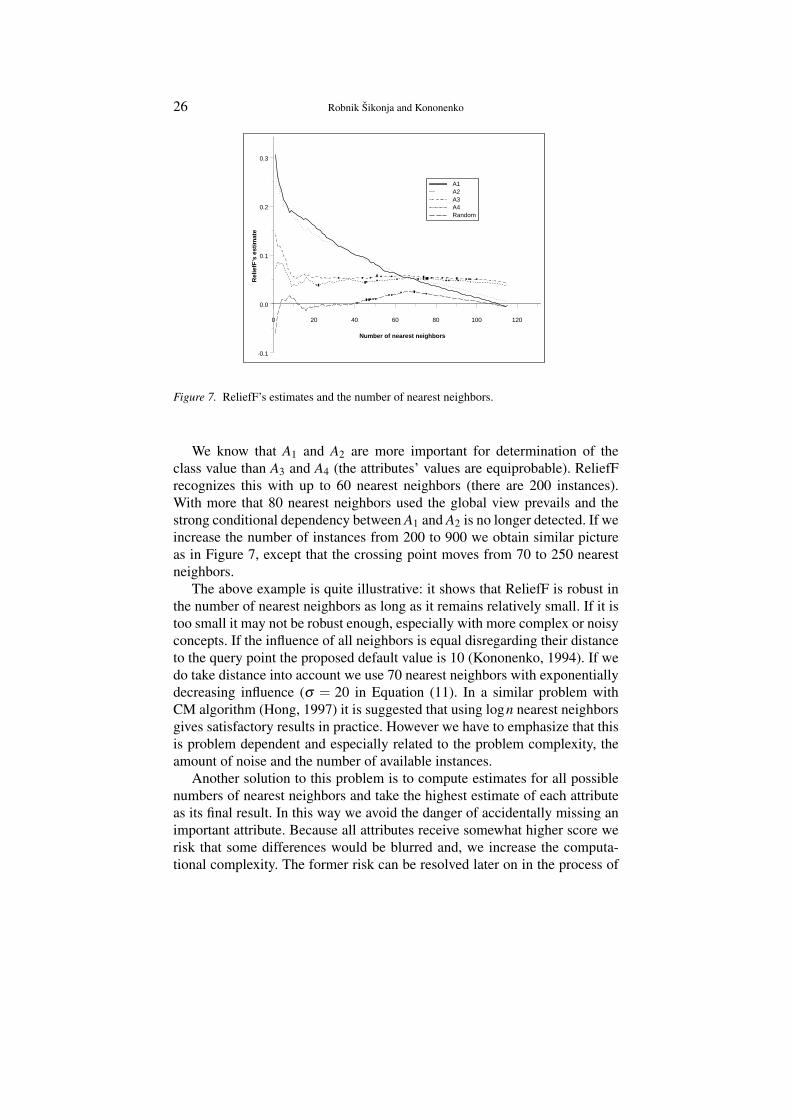
While the number of nearest neighbors used is related to the distance asdescribed above there are still some other issues to be discussed, namelyhow sensitive Relief algorithms are to the number of nearest neighbors used(lines 4,5, and 6 in Figure 2 and line 4 in Figure 3). The optimal number ofthe nearest neighbors used is problem dependent as we illustrate in Figure 7which shows ReliefF’s estimates for four important and one of the randomattributes in Boolean domain defined as:
Bool−Simple : C = (A1⊕A2)∨ (A3∧A4). (38)
26 Robnik Sikonja and Kononenko
0 20 40 60 80 100 120
Number of nearest neighbors
-0.1
0.0
0.1
0.2
0.3
Rel
iefF
’s e
stim
ate
A1A2A3A4Random
Figure 7. ReliefF’s estimates and the number of nearest neighbors.
We know that A1 and A2 are more important for determination of theclass value than A3 and A4 (the attributes’ values are equiprobable). ReliefFrecognizes this with up to 60 nearest neighbors (there are 200 instances).With more that 80 nearest neighbors used the global view prevails and thestrong conditional dependency between A1 and A2 is no longer detected. If weincrease the number of instances from 200 to 900 we obtain similar pictureas in Figure 7, except that the crossing point moves from 70 to 250 nearestneighbors.
The above example is quite illustrative: it shows that ReliefF is robust inthe number of nearest neighbors as long as it remains relatively small. If it istoo small it may not be robust enough, especially with more complex or noisyconcepts. If the influence of all neighbors is equal disregarding their distanceto the query point the proposed default value is 10 (Kononenko, 1994). If wedo take distance into account we use 70 nearest neighbors with exponentiallydecreasing influence (σ = 20 in Equation (11). In a similar problem withCM algorithm (Hong, 1997) it is suggested that using logn nearest neighborsgives satisfactory results in practice. However we have to emphasize that thisis problem dependent and especially related to the problem complexity, theamount of noise and the number of available instances.
Another solution to this problem is to compute estimates for all possiblenumbers of nearest neighbors and take the highest estimate of each attributeas its final result. In this way we avoid the danger of accidentally missing animportant attribute. Because all attributes receive somewhat higher score werisk that some differences would be blurred and, we increase the computa-tional complexity. The former risk can be resolved later on in the process of

Theoretical and Empirical Analysis of ReliefF and RReliefF 27
investigating the domain by producing a graph similar to Figure 7 showingdependencies of ReliefF’s estimates on the number of nearest neighbors. Thecomputational complexity increases from O(m ·n ·a) to O(m ·n · (a + logn))due to sorting of the instances with decreasing distance. In the algorithm wehave to do also some additional bookkeeping, e.g., keep the score for eachattribute and each number of nearest instances.
3.5. SAMPLE SIZE AND NUMBER OF ITERATIONS
Estimates of Relief algorithms are actually statistical estimates i.e., the al-gorithms collect the evidence for (non)separation of similar instances by theattribute across the problem space. To provide reliable estimates the coverageof the problem space must be appropriate. The sample has to cover enoughrepresentative boundaries between the prediction values. There is an obvioustrade off between the use of more instances and the efficiency of computa-tion. Wherever we have large datasets sampling is one of possible solutionsto make problem tractable. If a dataset is reasonably large and we want tospeed-up computations we suggest selection of all the available instances (nin complexity calculations), and rather to control the number of iterationswith parameter m (line 2 in Figures 2 and 3). As it is non trivial to select arepresentative sample of the unknown problem space our decision is in favorof the (possibly) sparse coverage of the more representative space rather thanthe dense coverage of the (possibly) non-representative sample.
0 100 200 300 400
Number of iterations
-0.2
-0.1
0.0
0.1
0.2
0.3
RR
elie
fF’s
est
imat
e
A1A2A3Random1Random2
Figure 8. RReliefF’s estimates and the number of iterations (m) on Cosinus-Lin dataset.
Figure 8 illustrates the behavior of RReliefF’s estimates changing withthe number of iterations on Cosinus-Lin dataset with 10 random attributes

28 Robnik Sikonja and Kononenko
and 1000 examples. We see that after the initial variation at around 20 itera-tions the estimates settle to stable values, except for difficulties at detectingdifferences e.g., the quality difference between A1 and A3 is not resolveduntil around 300 iterations (A1 within the cosine function controls the signof the expression, while A3 with the coefficient 3 controls the amplitude ofthe function). We should note that this is quite typical behavior and usuallywe get stable estimates after 20-50 iterations. However if we want to refinethe estimates we have to iterate further on. The question of how much moreiterations we need is problem dependent. We try to answer this question forsome chosen problems in Section 4.5.
4. Analysis of performance
In this Section we investigate some practical issues on the use of ReliefFand RReliefF: what kind of dependencies they detect, how do they scaleup to large number of examples and features, how many iterations we needfor reliable estimation, how robust are they regarding the noise, and howirrelevant and duplicate attributes influence their output. For ReliefF someof these questions have been tackled in a limited scope in (Kononenko, 1994;Kononenko et al., 1997) and for RReliefF in (Robnik Sikonja and Kononenko,1997).
Before we analyze these issues we have to define some useful measuresand concepts for performance analysis, comparison and explanation.
4.1. USEFUL DEFINITIONS AND CONCEPTS
4.1.1. Concept variationWe are going to examine abilities of ReliefF and ReliefF to recognize andrank important attributes for a set of different problems. As Relief algo-rithms are based on the nearest neighbor paradigm they are capable to detectclasses of problems for which this paradigm holds. Therefore we will definea measure of concept difficulty, called concept variation, based on the nearestneighbor principle.
Concept variation (Rendell and Seshu, 1990) is a measure of problem dif-ficulty based on the nearest neighbor paradigm. If many pairs of neighboringexamples do not belong to the same class, then the variation is high and theproblem is difficult (Perez and Rendell, 1996; Vilalta, 1999). It is defined ona-dimensional Boolean concepts as
Va =1
a2a
a
∑i=1
∑neigh(X ,Y,i)
diff(C,X ,Y ) (39)
where the inner summation is taken over all 2a pairs of the neighboring in-stances X and Y that differ only in their i-th attribute. Division by a2a converts
Theoretical and Empirical Analysis of ReliefF and RReliefF 29
double sum to average and normalizes the variation to [0,1] range. The twoconstant concepts (which have all class values 0 and 1, respectively) havevariation 0, and the two parity concepts of order a have variation 1. Randomconcepts have variation around 0.5, because the neighbors of any given ex-ample are approximately evenly split between the two classes. The variationaround 0.5 can be thus considered as high and the problem as difficult.
This definition of the concept variation is limited to Boolean problems anddemands the description of the whole problem space. The modified definitionby (Vilalta, 1999) encompasses the same idea but is defined also for numericand non-binary attributes. It uses only a sample of examples, which makesvariation possible to compute in the real world problems as well. Insteadof all pairs of the nearest examples it uses a distance metric to weight thecontribution of each example to the concept variation. The problem with thisdefinition is that it uses the contributions of all instances and thereby loosesthe information on locality. We propose another definition which borrowsfrom both mentioned above.
V =1
m ·am
∑i=1
a
∑j=1
diff(C,neigh(Xi,Y, j)) (40)
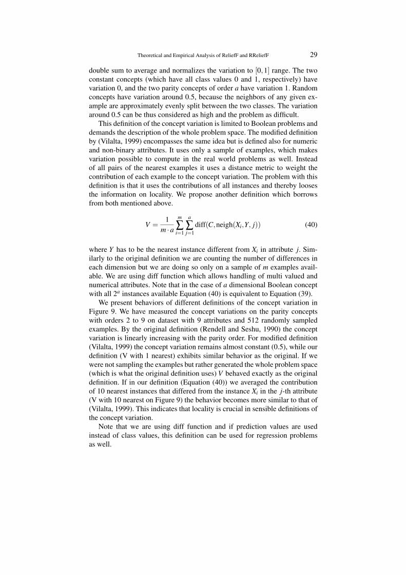
where Y has to be the nearest instance different from Xi in attribute j. Sim-ilarly to the original definition we are counting the number of differences ineach dimension but we are doing so only on a sample of m examples avail-able. We are using diff function which allows handling of multi valued andnumerical attributes. Note that in the case of a dimensional Boolean conceptwith all 2a instances available Equation (40) is equivalent to Equation (39).
We present behaviors of different definitions of the concept variation inFigure 9. We have measured the concept variations on the parity conceptswith orders 2 to 9 on dataset with 9 attributes and 512 randomly sampledexamples. By the original definition (Rendell and Seshu, 1990) the conceptvariation is linearly increasing with the parity order. For modified definition(Vilalta, 1999) the concept variation remains almost constant (0.5), while ourdefinition (V with 1 nearest) exhibits similar behavior as the original. If wewere not sampling the examples but rather generated the whole problem space(which is what the original definition uses) V behaved exactly as the originaldefinition. If in our definition (Equation (40)) we averaged the contributionof 10 nearest instances that differed from the instance Xi in the j-th attribute(V with 10 nearest on Figure 9) the behavior becomes more similar to that of(Vilalta, 1999). This indicates that locality is crucial in sensible definitions ofthe concept variation.
Note that we are using diff function and if prediction values are usedinstead of class values, this definition can be used for regression problemsas well.

30 Robnik Sikonja and Kononenko
2 3 4 5 6 7 8 9
parity order
0.0
0.2
0.4
0.6
0.8
1.0
con
cep
t va
riat
ion
(Rendell & Seshu, 1990)(Vilalta, 1999)V with 1 nearestV with 10 nearest
Figure 9. Concept variation by different definitions on parity concepts of orders 2 to 9 and512 examples.
4.1.2. Performance measuresIn our experimental scenario below we run ReliefF and RReliefF on a numberof different problems and observe
− if their estimates distinguish between important attributes (conveyingsome information about the concept) and unimportant attributes and
− if their estimates rank important attributes correctly (attributes whichhave stronger influence on prediction values should be ranked higher).
In estimating the success of Relief algorithms we use the following measures:
Separability s is the difference between the lowest estimate of the importantattributes and the highest estimate of the unimportant attributes.
s = WIworst −WRbest (41)
We say that a heuristics is successful in separating between the importantand unimportant attributes if s > 0.
Usability u is the difference between the highest estimates of the importantand unimportant attributes.
u = WIbest −WRbest (42)
We say that estimates are useful if u is greater than 0 (we are gettingat least some information from the estimates e.g., the best importantattribute could be used as the split in tree based model). It holds thatu≥ s.

Theoretical and Empirical Analysis of ReliefF and RReliefF 31
4.1.3. Other attribute estimators for comparisonFor some problems we want to compare the performance of ReliefF andRReliefF with other attribute estimation heuristics. We have chosen the mostwidely used. For classification this is the gain ratio (used in e.g., C4.5 (Quin-lan, 1993)) and for regression it is the mean squared error (MSE) of averageprediction value (used in e.g., CART (Breiman et al., 1984)).
Note that MSE, unlike Relief algorithms and gain ratio, assigns lowerweights to better attributes. To make s and u curves comparable to that ofRReliefF we are actually reporting separability and usability with the signreversed.
4.2. SOME TYPICAL PROBLEMS AND DEPENDENCIES
We use artificial datasets in the empirical analysis because we want to con-trol the environment: in real-world datasets we do not fully understand theproblem and the relation of the attributes to the target variable. Thereforewe do not know what a correct output of the feature estimation should beand we cannot evaluate the quality estimates of the algorithms. We mostlyuse variants of parity-like problems because these are the most difficult prob-lems within the nearest neighbor paradigm. We try to control difficulty ofthe concepts (which we measure with the concept variation) and therefore weintroduce many variants with various degrees of the concept variation. We usealso some non-parity like problems and demonstrate performances of Reliefalgorithms on them. We did not find another conceptually different class ofproblems on which the Relief algorithms would exhibit significantly differentbehavior.
4.2.1. Sum by modulo conceptsWe start our presentation of abilities of ReliefF and RReliefF with the con-cepts based on summation by modulo. Sum by modulo p problems are integergeneralizations of parity concept, which is a special case where attributesare Boolean and the class is defined by modulo 2. In general, each Modulo-p-I problem is described by a set of attributes with integer values in therange [0, p). The predicted value τ(X) is the sum of I important attributesby modulo p.
Modulo−p−I : τ(X) = (I
∑i=1
Xi) mod p (43)
Let us start with the base case i.e., Boolean problems (p = 2). As an illus-trative example we will show problems with parity of 2-8 attributes (I ∈ [2,8])on the data set described with 9 attributes and 512 examples (a completedescription of the domain). Figure 10 shows s curve for this problem (u curve

32 Robnik Sikonja and Kononenko
is identical as we have a complete description of a domain). In this and allfigures below each point on the graph is an average of 10 runs.
We can see that separability of the attributes is decreasing with increasingdifficulty of the problem for parity orders of 2,3, and 4. At order 5 when morethan half of the attributes are important the separability becomes negativei.e., we are no longer capable of separating the important from unimportantattributes. The reason is that we are using more than one nearest neighbor(one nearest neighbor would always produce positive s curve on this noise-less problem) and as the number of peaks in the problem increases with2I , and the number of examples remains constant (512) we are having lessand less examples per peak. At I = 5 when we get negative s the numberof nearest examples from the neighboring peaks with distance 1 (differentparity) surpasses the number of nearest examples from the target peak. Aninteresting point to note is when I = 8 (there is only 1 random attribute left)and s becomes positive again. The reason for this is that the number of nearestexamples from the target peak and neighboring peaks with distance 2 (withthe same parity!) surpasses the number of nearest examples from neighboringpeaks with distance 1 (different parity).
2 3 4 5 6 7 8
parity order-0.10
0.00
0.10
0.20
0.30
0.40
0.50
sep
arab
ility
Figure 10. Separability on parity concepts of orders 2 to 8 and all 512 examples.
A sufficient number of examples per peak is crucial for reliable estima-tions with ReliefF as we show in Figure 11. The bottom s and u curves showexactly the same problem as above (in Figure 10) but in this case the problemis not described with all 512 examples but rather with 512 randomly generatedexamples. The s scores are slightly lower than in Figure 10 as we have ineffect decreased the number of different examples (to 63.2% of the total). Thetop s and u curves show the same problem but with 8 times more examples

Theoretical and Empirical Analysis of ReliefF and RReliefF 33
2 3 4 5 6 7 8
parity order-0.10
0.00
0.10
0.20
0.30
0.40
0.50
sep
arab
ility
, usa
bili
ty
separability on 4096examplesusability on 4096 examplesseparability on 512 examplesusability on 512 examples
Figure 11. Separability and usability on parity concepts of orders 2 to 8 and randomly sampled512 or 4096 examples.
(4096). We can observe that with that many examples the separability for allproblems is positive.
In the next problem p increases while the number of important attributesand the number of examples are fixed (to 2 and 512, respectively).
0 10 20 30 40 50
modulo-0.10
0.00
0.10
0.20
0.30
0.40
0.50
sep
arab
ility
regression problem with nominal attributesregression problem with numerical attributesclassification problem with nominal attributesclassification problem with numerical attributes
Figure 12. Separability for ReliefF and RReliefF on modulo classification and regressionproblems with changing modulo.
Two curves at the bottom of Figure 12 show separability (usability is verysimilar and is omitted due to clarity) for the classification problem (there are

34 Robnik Sikonja and Kononenko
0 1 2 3 4 5 6Number of important attributes
0.00
0.10
0.20
0.30
0.40
0.50
sep
arab
ility
Classification problemsRegression problems
Figure 13. Separability for ReliefF and RReliefF on modulo 5 problems with changing thenumber of important attributes.
p classes) and thus we can see the performance of ReliefF. The attributes canbe treated as nominal or numerical, however, the two curves show similarbehavior i.e., separability is decreasing with increasing modulo. This is ex-pected as the complexity of problems is increasing with the number of classes,attribute values, and peaks. The number of attributes values and classes is in-creasing with p, while the number of peaks is increasing with pI (polynomialincrease). Again, more examples would shift positive values of s further to theright. A slight but important difference between separability for nominal andnumerical attributes shows that numerical attributes convey more informationin this problem. Function diff is 1 for any two different nominal attributeswhile for numerical attributes diff returns the relative numerical differencewhich is more informative.
The same modulo problems can be viewed as regression problems and theattributes can be again interpreted as nominal or numerical. Two curves atthe top of Figure 12 shows separability for the modulo problem formulatedas regression problem (RReliefF is used). We get positive s values for largermodulo compared to the classification problem and if the attributes are treatedas numerical the separability is not decreasing with modulo at all. The reasonis that classification problems were actually more difficult. We tried to predictp separate classes (e.g., results 2 and 3 are completely different in classifica-tion) while in regression we model numerical values (2 and 3 are differentrelatively to the scale).
Another interesting problem arises if we fix modulo to a small number(e.g., p = 5) and vary the number of important attributes. Figure 13 shows
Theoretical and Empirical Analysis of ReliefF and RReliefF 35
s curves for 4096 examples and 10 random attributes. At modulo 5 there areno visible differences in the performance for nominal and numerical attributestherefore we give curves for nominal attributes only. The s curves are decreas-ing rapidly with increasing I. Note that the problem complexity (number ofpeaks) is increasing with pI (exponentially).
Modulo problems are examples of difficult problems in the sense that theirconcept variation is high. Note that impurity-based measures such as Gainratio, are not capable of separating important from random attributes for anyof the above described problems.
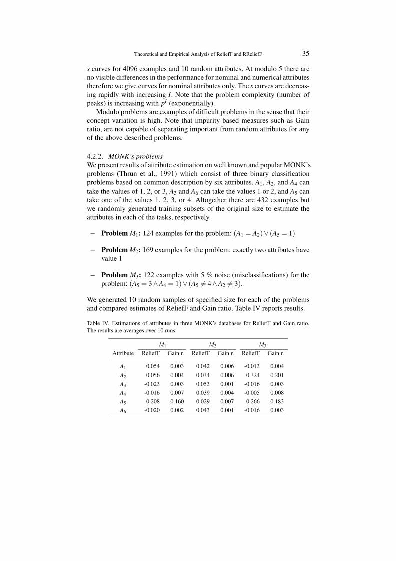
4.2.2. MONK’s problemsWe present results of attribute estimation on well known and popular MONK’sproblems (Thrun et al., 1991) which consist of three binary classificationproblems based on common description by six attributes. A1, A2, and A4 cantake the values of 1, 2, or 3, A3 and A6 can take the values 1 or 2, and A5 cantake one of the values 1, 2, 3, or 4. Altogether there are 432 examples butwe randomly generated training subsets of the original size to estimate theattributes in each of the tasks, respectively.
− Problem M1: 124 examples for the problem: (A1 = A2)∨ (A5 = 1)
− Problem M2: 169 examples for the problem: exactly two attributes havevalue 1
− Problem M3: 122 examples with 5 % noise (misclassifications) for theproblem: (A5 = 3∧A4 = 1)∨ (A5 6= 4∧A2 6= 3).
We generated 10 random samples of specified size for each of the problemsand compared estimates of ReliefF and Gain ratio. Table IV reports results.
Table IV. Estimations of attributes in three MONK’s databases for ReliefF and Gain ratio.The results are averages over 10 runs.
M1 M2 M3
Attribute ReliefF Gain r. ReliefF Gain r. ReliefF Gain r.
A1 0.054 0.003 0.042 0.006 -0.013 0.004A2 0.056 0.004 0.034 0.006 0.324 0.201A3 -0.023 0.003 0.053 0.001 -0.016 0.003A4 -0.016 0.007 0.039 0.004 -0.005 0.008A5 0.208 0.160 0.029 0.007 0.266 0.183A6 -0.020 0.002 0.043 0.001 -0.016 0.003

36 Robnik Sikonja and Kononenko
For the first problem we see that ReliefF separates the important attributes(A1, A2, and A5) from unimportant ones while Gain ratio does not recognizeA1 and A2 as important attributes in this task.
In the second problem where all the attributes are important ReliefF as-signs them all positive weights. It favors attributes with less values as theyconvey more information. Gain ratio does the opposite: it favors attributeswith more values.
In the third problem ReliefF and gain ratio behave similarly: they separateimportant attributes from unimportant ones and rank them equally (A2, A5,and A4).
4.2.3. Linear and nonlinear problemsIn typical regression problems linear dependencies are mixed with some non-linear dependencies. We investigate problems of such type. The problemsare described with numerical attributes with values from the [0,1] intervaland 1000 instances. Besides I important attributes there are also 10 randomattributes in each problem.
We start with linear dependencies and create problems of the form:
LinInc−I : τ =I
∑j=1
j ·A j (44)
The attributes with larger coefficient have stronger influence on the pre-diction value and should be estimated as more important.
Table V. Estimations of the best random attribute (Rbest ) and all informative attributes inLinInc-I problems for RReliefF (RRF) and MSE. RReliefF assigns higher scores and MSEassigns lower scores to better attributes.
LinInc-2 LinInc-3 LinInc-4 LinInc-5Attr. RRF MSE RRF MSE RRF MSE RRF MSE
Rbest -0.040 0.424 -0.023 1.098 -0.009 2.421 -0.010 4.361A1 0.230 0.345 0.028 1.021 -0.018 2.342 -0.007 4.373A2 0.461 0.163 0.154 0.894 0.029 2.093 0.014 4.181A3 0.286 0.572 0.110 1.833 0.039 3.777A4 0.180 1.508 0.054 3.380A5 0.139 2.837
Table V reports quality estimates of attributes for RReliefF and MSE. Wesee that for small differences between importance of attributes both RReliefFand MSE are successful in recognizing this and ranking them correctly. When

Theoretical and Empirical Analysis of ReliefF and RReliefF 37
1 2 3 4 5 6 7 8 9
number of important attributes I
0.00
0.20
0.40
0.60
0.80
1.00
sep
arab
ility
, usa
bili
ty
separability for RReliefFusability for RReliefFseparability for MSEusability for MSE
Figure 14. Separability and usability on LinInc concepts for 1000 examples.
the differences between the importance of attributes become larger (in LinInc-4 and LinInc-5) it is possible due to random fluctuations in the data one of therandom attributes is estimated as better than the least important informativeattribute (A1). This happens in LinInc-4 for RReliefF and in LinInc-5 forMSE. The behavior of s and u are illustrated in Figure 14.
Another form of linear dependencies we are going to investigate is
LinEq−I : τ =I
∑j=1
A j (45)
Here all the attributes are given equal importance and we want to see howmany important attributes can we afford. Figure 15 shows separability andusability curves for RReliefF and MSE.
We see that separability is decreasing for RReliefF and becomes negativewith 10 important attributes. This is not surprising considering properties ofRelief: each attribute gets its weight according to the portion of explainedfunction values (see Section 2.7) so by increasing the number of importantattributes their weights decrease and approaches zero. The same is true forRReliefF’s usability which, however, becomes negative much later. MSE es-timates each attribute separately and is therefore not susceptible to this kind ofdefects, however, by increasing the number of important attributes the prob-ability to assign one of them a low score increases and so s curve becomesnegative. If we increase the number of examples to 4000, RReliefF’s s curvebecomes negative at 16 important attributes while the behavior of MSE doesnot change.
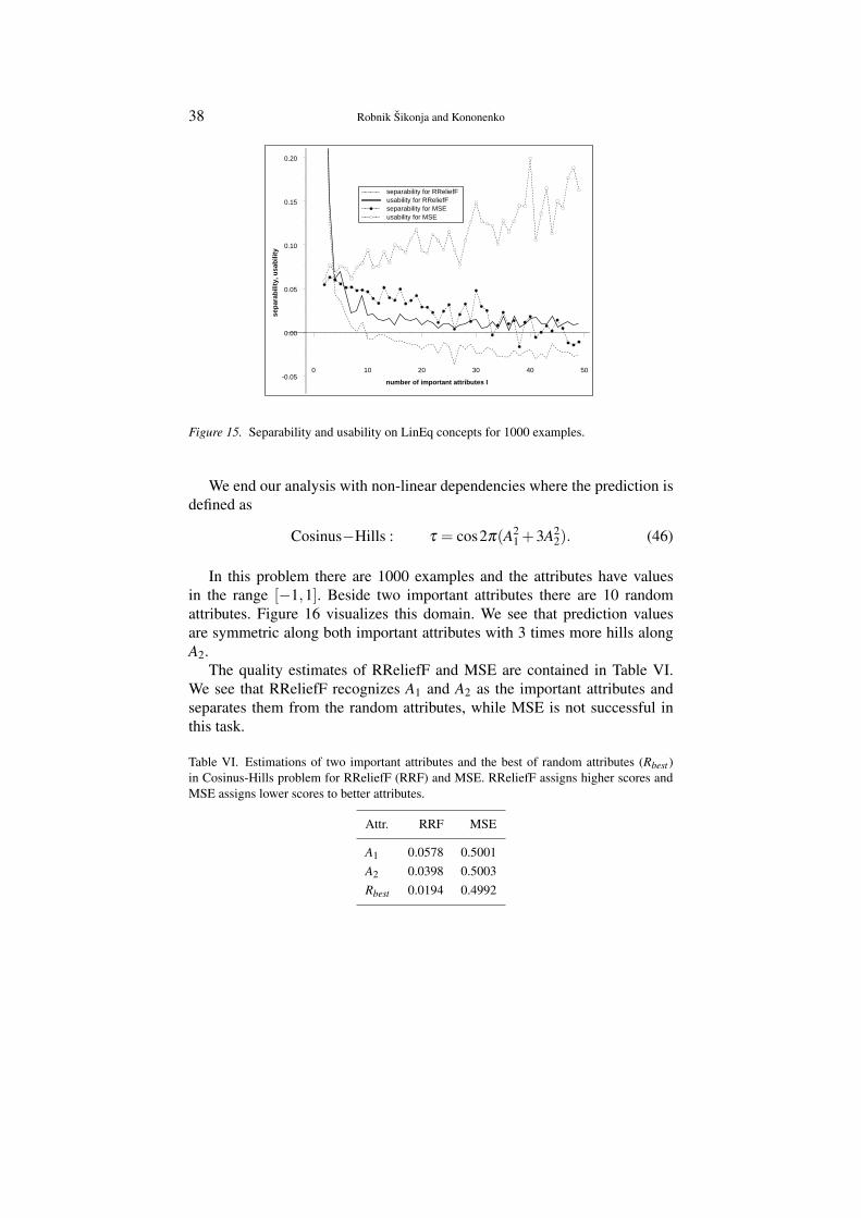
38 Robnik Sikonja and Kononenko
0 10 20 30 40 50
number of important attributes I-0.05
0.00
0.05
0.10
0.15
0.20
sep
arab
ility
, usa
bili
ty
separability for RReliefFusability for RReliefFseparability for MSEusability for MSE
Figure 15. Separability and usability on LinEq concepts for 1000 examples.
We end our analysis with non-linear dependencies where the prediction isdefined as
Cosinus−Hills : τ = cos2π(A21 +3A2
2). (46)
In this problem there are 1000 examples and the attributes have valuesin the range [−1,1]. Beside two important attributes there are 10 randomattributes. Figure 16 visualizes this domain. We see that prediction valuesare symmetric along both important attributes with 3 times more hills alongA2.
The quality estimates of RReliefF and MSE are contained in Table VI.We see that RReliefF recognizes A1 and A2 as the important attributes andseparates them from the random attributes, while MSE is not successful inthis task.
Table VI. Estimations of two important attributes and the best of random attributes (Rbest )in Cosinus-Hills problem for RReliefF (RRF) and MSE. RReliefF assigns higher scores andMSE assigns lower scores to better attributes.
Attr. RRF MSE
A1 0.0578 0.5001A2 0.0398 0.5003Rbest 0.0194 0.4992
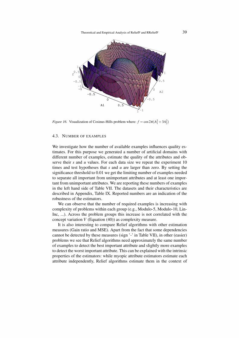
Theoretical and Empirical Analysis of ReliefF and RReliefF 39
-1
-0.5
0
0.5
1
A1
-1
-0.5
0
0.5
1
A2
-1
-0.5
0
0.5
1
f
-1
-0.5
0
0.5A1
Figure 16. Visualization of Cosinus-Hills problem where: f = cos2π(A21 +3A2
2)
4.3. NUMBER OF EXAMPLES
We investigate how the number of available examples influences quality es-timates. For this purpose we generated a number of artificial domains withdifferent number of examples, estimate the quality of the attributes and ob-serve their s and u values. For each data size we repeat the experiment 10times and test hypotheses that s and u are larger than zero. By setting thesignificance threshold to 0.01 we get the limiting number of examples neededto separate all important from unimportant attributes and at least one impor-tant from unimportant attributes. We are reporting these numbers of examplesin the left hand side of Table VII. The datasets and their characteristics aredescribed in Appendix, Table IX. Reported numbers are an indication of therobustness of the estimators.
We can observe that the number of required examples is increasing withcomplexity of problems within each group (e.g., Modulo-5, Modulo-10, Lin-Inc, ...). Across the problem groups this increase is not correlated with theconcept variation V (Equation (40)) as complexity measure.
It is also interesting to compare Relief algorithms with other estimationmeasures (Gain ratio and MSE). Apart from the fact that some dependenciescannot be detected by these measures (sign ’-’ in Table VII), in other (easier)problems we see that Relief algorithms need approximately the same numberof examples to detect the best important attribute and slightly more examplesto detect the worst important attribute. This can be explained with the intrinsicproperties of the estimators: while myopic attribute estimators estimate eachattribute independently, Relief algorithms estimate them in the context of

40 Robnik Sikonja and Kononenko
Table VII. Results of varying the number of examples and noisy prediction value.
Number of examples NoiseReliefF Gain r. ReliefF Gain r.
Name s u s u s u s u
Bool-Simple 100 50 - 40 10 45 - 20Modulo-2-2-c 70 60 - - 30 50 - -Modulo-2-3-c 170 110 - - 5 50 - -Modulo-2-4-c 550 400 - - 20 50 - -Modulo-5-2-c 150 130 - - 5 5 - -Modulo-5-3-c 950 800 - - 15 35 - -Modulo-5-4-c 5000 4000 - - 10 50 - -Modulo-10-2-c 400 400 - - 20 20 - -Modulo-10-3-c 4000 3000 - - 25 55 - -Modulo-10-4-c 25000 22000 - - 10 40 - -MONK-1 100 30 - 20 30 70 - 55MONK-3 250 10 250 20 25 75 5 75
RReliefF MSE RReliefF MSEModulo-5-2-r 60 50 - - 25 50 - -Modulo-5-3-r 400 350 - - 20 45 - -Modulo-5-4-r 2000 1600 - - 15 40 - -Modulo-10-2-r 90 80 - - 25 40 - -Modulo-10-3-r 800 600 - - 10 40 - -Modulo-10-4-r 7000 4000 - - 5 40 - -Fraction-2 80 70 - - 20 40 - -Fraction-3 650 400 - - 15 35 - -Fraction-4 4000 3000 - - 10 35 - -LinInc-2 60 10 70 20 15 50 10 50LinInc-3 400 20 150 10 10 65 20 70LinInc-4 2000 40 450 10 5 80 35 85LinEq-2 50 40 20 20 30 60 25 45LinEq-3 180 50 50 20 25 40 30 50LinEq-4 350 70 70 30 10 40 30 45Cosinus-Lin 300 40 - 200 15 50 - 40Cosinus-Hills 550 300 4000 2000 5 20 - -
other attributes, i.e., all important attributes share the positive estimate andbetter attributes get more.

Theoretical and Empirical Analysis of ReliefF and RReliefF 41
4.4. ADDING NOISE BY CHANGING PREDICTED VALUE
We check robustness of Relief algorithms concerning by using the same set-ting as before with the number of examples from the first s column in theleft-hand side of Table VII. We added noise to the data sets by changingcertain percent of predicted values to a random value. We varied the noisefrom 0 to 100% in 5% steps.
The right-hand side of Table VII gives the maximal percentage of cor-rupted prediction values where s and u were still positive with high probabil-ity (> 0.99).
We can observe that Relief algorithms are quite concerning the noise inall the problems. When we increase the number of examples 10 times we areable to randomly set more than 80% of values in every problem. Comparisonwith myopic measures (Gain ratio and MSE) is included in two right-handcolumns. We see that in problems where these measures are successful theirnoise tolerance is comparable with Relief algorithms.
4.5. NUMBER OF ITERATIONS
We check how many iterations Relief algorithms need to compute by usingthe same setting as above. The left-hand side of Table VIII gives a minimalnumber of iterations needed in each problem so that s and u are positive withprobability > 0.99. The columns labelled ’#Ex’ are results for the number ofexamples fixed to the number of examples from the first s column in TableVII, and two columns labelled ’10× #Ex’ contain results for 10 times thatmany examples.
There are two interesting observations. The first is that even with the min-imal number of examples needed for distinguishing two sets of attributes wedo not need to do that many iterations and the actual number of iterations issometimes quite low. And secondly, if we have an abundance of examplesavailable than we can afford to do only very little iterations as seen from the’10× #Ex’ columns in Table VIII.
4.6. ADDING MORE RANDOM ATTRIBUTES
ReliefF and RReliefF are context sensitive and take all attributes into accountwhen estimating their quality. They are therefore more sensitive to abundanceof random attributes than myopic measures, which estimate each attributeseparately. We test this sensitivity with similar settings as before (defaultparameters, the number of examples from the first s column in Table VII)and add various numbers of randomly generated attributes.
Right-hand side of Table VIII summarizes results (we consider MONK’sdata sets fixed and did not include them in this test - label NA). The twocolumns give the maximal number of random attributes that can be added
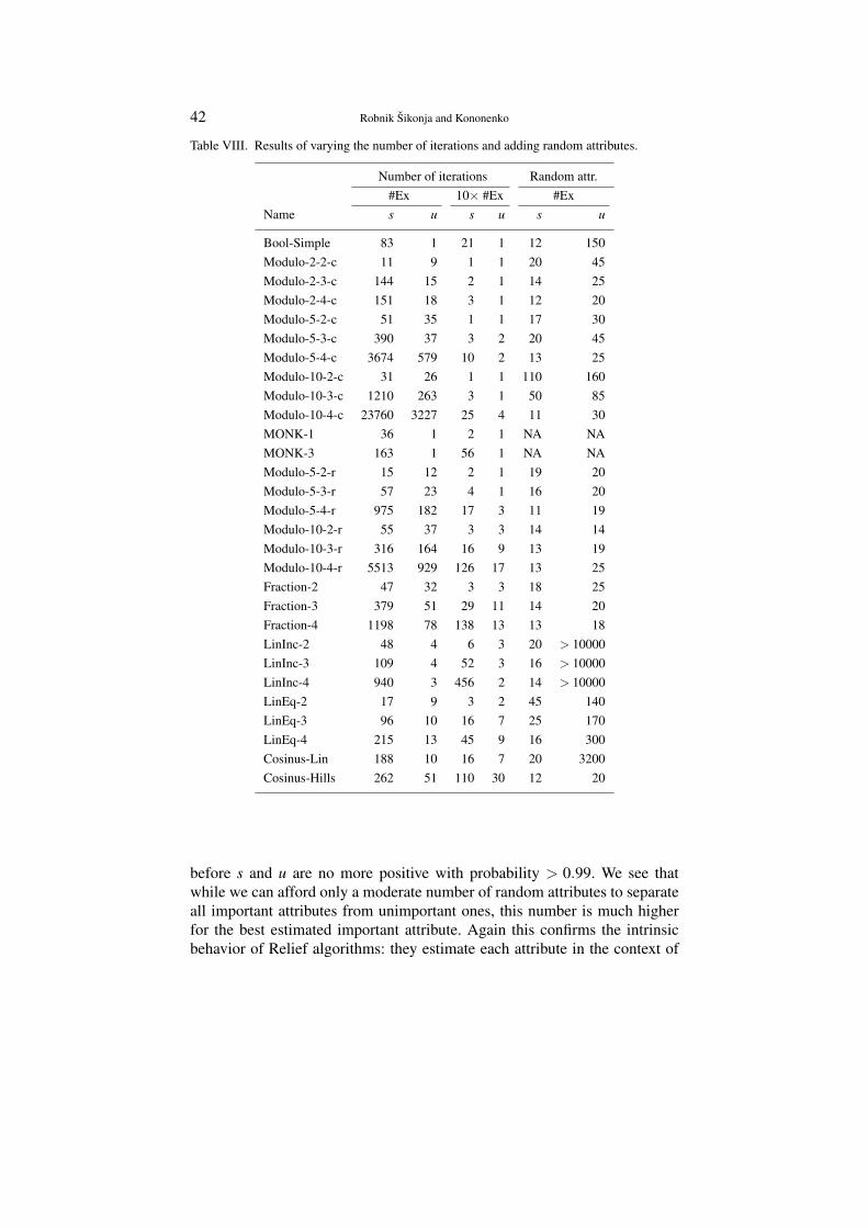
42 Robnik Sikonja and Kononenko
Table VIII. Results of varying the number of iterations and adding random attributes.
Number of iterations Random attr.#Ex 10× #Ex #Ex
Name s u s u s u
Bool-Simple 83 1 21 1 12 150Modulo-2-2-c 11 9 1 1 20 45Modulo-2-3-c 144 15 2 1 14 25Modulo-2-4-c 151 18 3 1 12 20Modulo-5-2-c 51 35 1 1 17 30Modulo-5-3-c 390 37 3 2 20 45Modulo-5-4-c 3674 579 10 2 13 25Modulo-10-2-c 31 26 1 1 110 160Modulo-10-3-c 1210 263 3 1 50 85Modulo-10-4-c 23760 3227 25 4 11 30MONK-1 36 1 2 1 NA NAMONK-3 163 1 56 1 NA NAModulo-5-2-r 15 12 2 1 19 20Modulo-5-3-r 57 23 4 1 16 20Modulo-5-4-r 975 182 17 3 11 19Modulo-10-2-r 55 37 3 3 14 14Modulo-10-3-r 316 164 16 9 13 19Modulo-10-4-r 5513 929 126 17 13 25Fraction-2 47 32 3 3 18 25Fraction-3 379 51 29 11 14 20Fraction-4 1198 78 138 13 13 18LinInc-2 48 4 6 3 20 > 10000LinInc-3 109 4 52 3 16 > 10000LinInc-4 940 3 456 2 14 > 10000LinEq-2 17 9 3 2 45 140LinEq-3 96 10 16 7 25 170LinEq-4 215 13 45 9 16 300Cosinus-Lin 188 10 16 7 20 3200Cosinus-Hills 262 51 110 30 12 20
before s and u are no more positive with probability > 0.99. We see thatwhile we can afford only a moderate number of random attributes to separateall important attributes from unimportant ones, this number is much higherfor the best estimated important attribute. Again this confirms the intrinsicbehavior of Relief algorithms: they estimate each attribute in the context of
Theoretical and Empirical Analysis of ReliefF and RReliefF 43
other attributes and better attributes get higher score. This can be clearly seenin Lin-Inc and Cosinus-Lin domains where the important attributes are not allequally important.
Since MSE and Gain ratio are less sensitive to this kind of noise (only tothe extent that the probability of virtually ’good’ random attribute increaseswith more random attributes) we did not include them into this experiment.
4.7. NUMBER OF IMPORTANT ATTRIBUTES
Although the answer to the question, how many important attributes in do-main Relief algorithms can handle, is already contained in previous sec-tions we will summarize the results here and give some explanations for thisimportant practical issue.
If important attributes are not equally important then Relief algorithmsideally would share the credit among them in proportion of the explainedconcept (see Eq. (24)). In practice (with limited number of examples) lessimportant attributes get less than this. The reason for this is that the dif-ferences in predicted value caused by less important attribute (see Eq. 12)are overshadowed by larger changes caused by more important attributes.The example of such behavior can be seen in Figure 14 and Table V whereattributes are not equally important. With four attributes in such conditionsthe separability was no longer positive for RReliefF. Usability on the otherhand is robust and remains positive even with several hundred of importantattributes.
If all attributes are equally important then we can afford somewhat largernumber of attributes still to get positive separability as illustrated in Figure 15.Note, however, that the exact number is strongly dependent on sufficient num-ber of examples to cover the problem space adequately. Again the usabilitystays positive even for several hundreds of important attributes.
In short, Relief algorithms tend to underestimate less important attributeswhile recognition of more important attributes in not questionable even indifficult conditions.
4.8. DUPLICATE ATTRIBUTES
We demonstrate behaviors of Relief algorithms in the presence of duplicateattributes. As a baseline we take a simple Boolean XOR problem with 2important and 10 random attributes with 1000 examples for which ReliefFreturns the following estimates:
I1 I2 Rbest
0.445 0.453 -0.032
Now we duplicate the first important attribute I1 and get:
44 Robnik Sikonja and Kononenko
I1,C1 I1,C2 I2 Rbest
0.221 0.221 0.768 -0.015
Both copies of I1 now share the estimate and I2 gets some additional credit.Before we explain these estimates we try with 3 copies of the first importantattribute:
I1,C1 I1,C2 I1,C3 I2 Rbest
0.055 0.055 0.055 0.944 -0.006
and also with 10 copies:
I1,C1 I1,C2 ... I1,C10 I2 Rbest
0.000 0.000 ... 0.000 1.000 0.006
The reason for this behavior is that the additional copies of the attributechange the problem space in which the nearest neighbors are searched. Recallthat for each instance the algorithm searches nearest neighbors with the sameprediction and nearest neighbors with different prediction and then updatesthe estimates according to the values of diff function (see Equation 1). Theupdates occur only when values of diff is non-zero i.e., when the attribute’svalues are different. The difference in c times multiplied attribute causes thatthe instances are now at least on the distance c which causes that this instancewill slip out of the near neighborhood of the observed instance. As a conse-quence the odds of the multiplied attribute to get any update are diminishingand its quality estimate converges towards zero. The reverse is true for non-multiplied attributes: they get more frequently into the near neighborhoodand are more frequently updated so the important attributes get higher scoreas deserved.
If all important attributes are multiplied (not very likely in practical prob-lems) then this effect disappears because the distances are symmetricallystretched. Here is an example with 10 copies of both important attributes:
I1,C1 ... I1,C10 I2,C1 ... I2,C10 Rbest
0.501 ... 0.501 0.499 ... 0.4999 -0.037
The conclusion is that Relief algorithms are sensitive to duplicated at-tributes because they change the problem space. We can also say that Reliefalgorithms give credit to attributes according to the amount of explained con-cept and if several attributes have to share the credit it is appropriately smallerfor each of them. Of course, myopic estimators such as Gain ratio and MSE,are not sensitive to duplicate attributes.

Theoretical and Empirical Analysis of ReliefF and RReliefF 45
5. Applications
In previous sections we browsed through theoretical and practical issues onthe use of Relief algorithms. In this section we try to give a short overviewof their applications. We begin with the feature subset selection and featureweighting which were the initial purposes of Relief algorithm and then con-tinue with the use of ReliefF and RReliefF in tree based models, discretizationof attributes, and in inductive logic programming.
5.1. FEATURE SUBSET SELECTION AND FEATURE WEIGHTING
Originally, the Relief algorithm was used for feature subset selection (Kiraand Rendell, 1992b; Kira and Rendell, 1992a) and it is considered one of thebest algorithms for this purpose (Dietterich, 1997). Feature subset selectionis a problem of choosing a small set of attributes that ideally is necessary andsufficient to describe the target concept.
To select the set of the most important attributes (Kira and Rendell, 1992a)introduced significance threshold θ . If weight of a given attribute is below θ itis considered unimportant and is excluded from the resulting set. Bounds forθ were proposed i.e., 0 < θ ≤ 1√
αm , where α is the probability of acceptingan irrelevant feature as relevant and m is the number of iterations used (seeFigure 1). The upper bound for θ is very loose and in practice much smallervalues can be used.
Feature weighting is an assignment of a weight (importance) to each fea-ture and can be viewed as a generalization of feature subset selection in thesense that it does not assign just binary weights (0-1, include-exclude) to eachfeature but rather an arbitrary real number can be assigned to it. If Relief algo-rithms are used in this fashion then we do not need a significance threshold butrather use their weights directly. ReliefF was tested as the feature weightingmethod in the lazy learning (Wettschereck et al., 1997) and was found to bevery useful.
5.2. BUILDING TREE BASED MODELS
In learning tree based models (decision or regression trees) in a top downmanner we need an attribute estimation procedure in each node of the tree todetermine the appropriate split. Commonly used estimators for this task areimpurity based e.g., Gini index (Breiman et al., 1984) or Gain ratio (Quin-lan, 1993) in classification and mean squared error (Breiman et al., 1984)in regression. While these estimators are myopic and cannot detect condi-tional dependencies between attributes they also have inappropriate bias con-cerning multi-valued attributes (Kononenko, 1995). ReliefF was successfully

46 Robnik Sikonja and Kononenko
employed in classification (Kononenko and Simec, 1995; Kononenko et al.,1997) and RReliefF in regression problems (Robnik Sikonja and Kononenko,1996; Robnik Sikonja and Kononenko, 1997)1. Relief algorithms perform asgood as myopic measures if there are no conditional dependencies amongthe attributes and clearly surpass them if there are strong dependencies. Weclaim that when faced with an unknown data set it is unreasonable to assumethat it contains no strong conditional dependencies and rely only on myopicattribute estimators. Furthermore, using impurity based estimator near thefringe of the decision tree leads to unoptimal splits concerning accuracy andswitch to accuracy has been suggested as a remedy (Brodley, 1995; Lubinsky,1995). It was shown (Robnik Sikonja and Kononenko, 1999) that ReliefF indecision trees as well as RReliefF in regression trees do not need such switchas they contain it implicitly.
We also employ Relief algorithms to guide the constructive inductionprocess during growing of the trees. Only the most promising attributes areselected for construction and various operators were applied on them (con-junction, disjunction, summation, product). The results are good and in somedomains the obtained constructs provided additional insight into the domain(Dalaka et al., 2000).
We also observe in our experiences with machine learning applications(medicine, ecology) that trees produced with Relief algorithms are more com-prehensible for human experts. Splits selected by them seem to mimic hu-man’s partition of the problem which we explain with the interpretation ofRelief’s weights as the portion of the explained concept (see Section 2.7).
5.3. DISCRETIZATION OF ATTRIBUTES
Discretization divides the values of a numerical attribute into a number ofintervals. Each interval can then be treated as one value of the new nomi-nal attribute. The purpose of discretization, which is viewed as an importantpreprocessing step in machine learning is multiple: some algorithms cannothandle numerical attributes and need discretization, it reduces computationalcomplexity and the splits may convey important information. While Reliefalgorithms are used for discretization in our tree learning system, the dis-cretization capability was analyzed separately for ReliefF in (Robnik, 1995).The discretization on artificial datasets showed that conditionally dependentattributes might have important boundaries, which cannot be detected bymyopic measures.
1 A learning system that contains ReliefF and RReliefF is freely available upon e-mailrequest to the authors.

Theoretical and Empirical Analysis of ReliefF and RReliefF 47
5.4. USE IN ILP AND WITH ASSOCIATION RULES
In inductive logic programming a variant of ReliefF algorithm was used toestimate the quality of literals, which are candidates for augmenting the cur-rent clause under construction when inducing the first order theories witha learning system (Pompe and Kononenko, 1995). To adjust to specifics ofestimating literals diff function has to be changed appropriately. The modifieddiff function is asymmetric. The learning system, which uses this version ofReliefF, obtains good results on many learning problems.
The use of ReliefF together with an association rules based classifier (Jo-vanoski and Lavrac, 1999) is connected also with feature subset selection.The adaptation of the algorithm to association rules changes diff function ina similar way as ReliefF in ILP.
6. Further work
Although there has been a lot of work done with Relief algorithms we thinkthat there are plenty left to do. In this Section we will discuss some ideasconcerning parallelization, use as anytime algorithm, applications in timeseries, in cost-sensitive problems, and in meta learning.
6.1. PARALLELIZATION OF RELIEF ALGORITHMS
While Relief algorithms are computationally more complex than some other(myopic) attribute estimation measures they also have a possible advantagehat they can be naturally split into several independent tasks which is a pre-requisite for successful parallelization of an algorithm. Each iteration of thealgorithm is a natural candidate for a separate process, which would turnRelief into the fine-grained parallel algorithm.
6.2. ANYTIME ALGORITHM AND TIME SERIES
Anytime algorithm is an algorithm, which has a result available at any timeand with more time or more data it just improves the result. We think that Re-lief algorithms can be viewed as anytime algorithms, namely in each iterationthey refine the result. As our experiments show (e.g., left-hand side of TableVIII) even after only few little iterations Relief algorithms already producesensible results. The problems we may encounter if we add more data duringthe processing, are in proper normalizations of updated weights.
Another idea worth considering is to observe changes in quality weightswhen we add more and more data. In this way it might be possible to detectsome important phases in the time series e.g., a change of context.
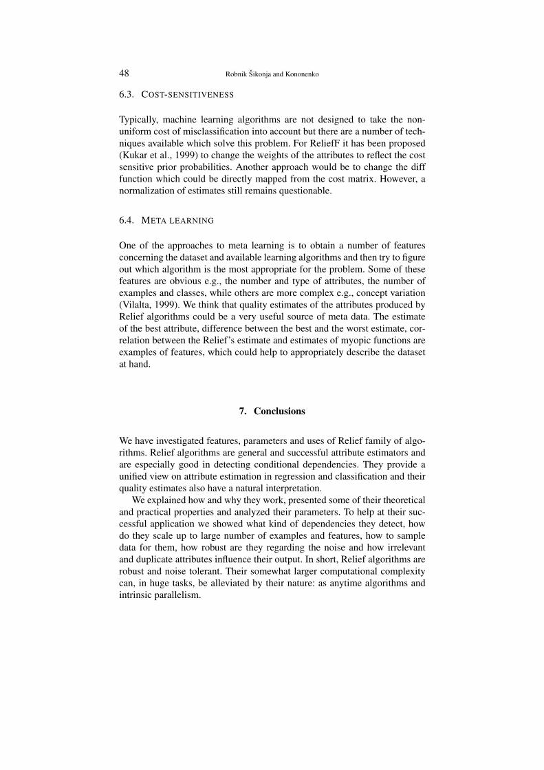
48 Robnik Sikonja and Kononenko
6.3. COST-SENSITIVENESS
Typically, machine learning algorithms are not designed to take the non-uniform cost of misclassification into account but there are a number of tech-niques available which solve this problem. For ReliefF it has been proposed(Kukar et al., 1999) to change the weights of the attributes to reflect the costsensitive prior probabilities. Another approach would be to change the difffunction which could be directly mapped from the cost matrix. However, anormalization of estimates still remains questionable.
6.4. META LEARNING
One of the approaches to meta learning is to obtain a number of featuresconcerning the dataset and available learning algorithms and then try to figureout which algorithm is the most appropriate for the problem. Some of thesefeatures are obvious e.g., the number and type of attributes, the number ofexamples and classes, while others are more complex e.g., concept variation(Vilalta, 1999). We think that quality estimates of the attributes produced byRelief algorithms could be a very useful source of meta data. The estimateof the best attribute, difference between the best and the worst estimate, cor-relation between the Relief’s estimate and estimates of myopic functions areexamples of features, which could help to appropriately describe the datasetat hand.
7. Conclusions
We have investigated features, parameters and uses of Relief family of algo-rithms. Relief algorithms are general and successful attribute estimators andare especially good in detecting conditional dependencies. They provide aunified view on attribute estimation in regression and classification and theirquality estimates also have a natural interpretation.
We explained how and why they work, presented some of their theoreticaland practical properties and analyzed their parameters. To help at their suc-cessful application we showed what kind of dependencies they detect, howdo they scale up to large number of examples and features, how to sampledata for them, how robust are they regarding the noise and how irrelevantand duplicate attributes influence their output. In short, Relief algorithms arerobust and noise tolerant. Their somewhat larger computational complexitycan, in huge tasks, be alleviated by their nature: as anytime algorithms andintrinsic parallelism.

Theoretical and Empirical Analysis of ReliefF and RReliefF 49
Appendix
The datasets
Some characteristics of the datasets, we used to demonstrate the features ofRelief algorithms, are contained in Table IX. For each domain we presentthe name, reference to where it was defined, number of classes or label thatit is regressional (r), number of important attributes (I), number of randomattributes (R), type of the attributes (nominal or numerical) and concept vari-ation V as a measure of concept difficulty (defined with Equation (40) andmeasured on 1000 examples - except for MONK-1 and MONK-3, where weused all 432 examples).
Some datasets are not explicitly defined in the text and we provide defini-tions here.
Cosinus-Lin is a non-linear dependency with cosine stretched over two pe-riods, multiplied by the linear combination of two attributes:
Cosinus−Lin : f = cos(4πA1) · (−2A2 +3A3) (47)
The attributes are numerical with values from 0 to 1.
Fraction-I is the same as the Modulo-∞-I domain with prediction and at-tributes normalized to [0,1]. It can be described as floating point gen-eralization of the parity concepts of order I with predicted values beingthe fractional part of the sum of I important attributes:
Fraction−I : f =I
∑j=1
A j−bI
∑j=1
A jc (48)
References
Bentley, J. L.: 1975, ‘Multidimensional Binary Search Trees Used for Associative Searching’.Communications of the ACM 15(9), 509–517.
Breiman, L., J. H. Friedman, R. A. Olshen, and C. J. Stone: 1984, Classification and regressiontrees. Belmont, California: Wadsworth Inc.
Brodley, C. E.: 1995, ‘Automatic Selection of Split Criterion during Tree Growing Basedon Node Location’. In: Machine Learning: Proceedings of the Twelfth InternationalConference (ICML’95). pp. 73–80, Morgan Kaufmann.
Cestnik, B., I. Kononenko, and I. Bratko: 1987, ‘ASSISTANT 86: A Knowledge-ElicitationTool for Sophisticated Users’. In: I. Bratko and N. Lavrac (eds.): Progress in MachineLearning, Proceedings of European Working Session on Learning EWSL’87. Wilmslow,pp. 31–36, Sigma Press.

50 Robnik Sikonja and Kononenko
Table IX. Short description of datasets.
Name Definition #class I R Attr. type V
Bool-Simple Equation (38) 2 4 10 nominal 0.283Modulo-2-2-c Equation (43) 2 2 10 nominal 0.278Modulo-2-3-c Equation (43) 2 3 10 nominal 0.379Modulo-2-4-c Equation (43) 2 4 10 nominal 0.444Modulo-5-2-c Equation (43) 5 2 10 nominal 0.651Modulo-5-3-c Equation (43) 5 3 10 nominal 0.748Modulo-5-4-c Equation (43) 5 4 10 nominal 0.790Modulo-10-2-c Equation (43) 10 2 10 numerical 0.808Modulo-10-3-c Equation (43) 10 3 10 numerical 0.891Modulo-10-4-c Equation (43) 10 4 10 numerical 0.902MONK-1 Section 4.2.2 2 3 3 nominal 0.213MONK-3 Section 4.2.2 2 3 3 nominal 0.145
Modulo-5-2-r Equation (43) r 2 10 nominal 0.658Modulo-5-3-r Equation (43) r 3 10 nominal 0.755Modulo-5-4-r Equation (43) r 4 10 nominal 0.803Modulo-10-2-r Equation (43) r 2 10 numerical 0.801Modulo-10-3-r Equation (43) r 3 10 numerical 0.885Modulo-10-4-r Equation (43) r 4 10 numerical 0.892Fraction-2 Equation (48) r 2 10 numerical 0.777Fraction-3 Equation (48) r 3 10 numerical 0.845Fraction-4 Equation (48) r 4 10 numerical 0.869LinInc-2 Equation (44) r 2 10 numerical 0.642LinInc-3 Equation (44) r 3 10 numerical 0.707LinInc-4 Equation (44) r 4 10 numerical 0.709LinEq-2 Equation (45) r 2 10 numerical 0.660LinEq-3 Equation (45) r 3 10 numerical 0.693LinEq-4 Equation (45) r 4 10 numerical 0.726Cosinus-Lin Equation (47) r 3 10 numerical 0.588Cosinus-Hills Equation (46) r 2 10 numerical 0.848
Dalaka, A., B. Kompare, M. Robnik-Sikonja, and S. Sgardelis: 2000, ‘Modeling the effectsof environmental conditions on apparent photosynthesis of Stipa bromoides by machinelearning tools’. Ecological Modelling 129, 245–257.
Deng, K. and A. W. Moore: 1995, ‘Multiresolution Instance-Based Learning’. In: Proceedingsof the International Joint Conference on Artificial Intelligence (IJCAI’95). pp. 1233–1239,Morgan Kaufmann.

Theoretical and Empirical Analysis of ReliefF and RReliefF 51
Dietterich, T. G.: 1997, ‘Machine Learning Research: Four Current Directions’. AI Magazine18(4), 97–136.
Domingos, P.: 1997, ‘Context-sensitive feature selection for lazy learners’. ArtificialIntelligence Review 11, 227–253.
Friedman, J. H., J. L. Bentley, and R. A. Finkel: 1975, ‘An algorithm for finding best matchesin logarithmic expected time’. Technical Report STAN-CS-75-482, Stanford University.
Hong, S. J.: 1994, ‘Use of contextual information for feature ranking and discretization’.Technical Report RC19664, IBM.
Hong, S. J.: 1997, ‘Use of Contextual Information for Feature Ranking and Discretization’.IEEE transactions on knowledge and data engineering 9(5), 718–730.
Hunt, E. B., J. Martin, and P. J. Stone: 1966, Experiments in Induction. New York: AcademicPress.
Jovanoski, V. and N. Lavrac: 1999, ‘Feature Subset Selection in Association Rules LearningSystems’. In: M. Grobelnik and D. Mladenic (eds.): Prooceedings of the ConferenceAnalysis, Warehousing and Mining the Data (AWAMIDA’99). pp. 74–77.
Kira, K. and L. A. Rendell: 1992a, ‘The feature selection problem: traditional methods andnew algorithm’. In: Proceedings of AAAI’92.
Kira, K. and L. A. Rendell: 1992b, ‘A practical approach to feature selection’. In: D.Sleemanand P.Edwards (eds.): Machine Learning: Proceedings of International Conference(ICML’92). pp. 249–256, Morgan Kaufmann.
Kononenko, I.: 1994, ‘Estimating attributes: analysis and extensions of Relief’. In: L.De Raedt and F. Bergadano (eds.): Machine Learning: ECML-94. pp. 171–182, SpringerVerlag.
Kononenko, I.: 1995, ‘On Biases in Estimating Multi-Valued Attributes’. In: Proceedings ofthe International Joint Conference on Aartificial Intelligence (IJCAI’95). pp. 1034–1040,Morgan Kaufmann.
Kononenko, I. and E. Simec: 1995, ‘Induction of decision trees using ReliefF’. In: G.Della Riccia, R. Kruse, and R. Viertl (eds.): Mathematical and Statistical Methods inArtificial Intelligence, CISM Courses and Lectures No. 363. Springer Verlag.
Kononenko, I., E. Simec, and M. Robnik-Sikonja: 1997, ‘Overcoming the Myopia of InductiveLearning Algorithms with RELIEFF’. Applied Intelligence 7, 39–55.
Kukar, M., I. Kononenko, C. Groselj, K. Kralj, and J. Fettich: 1999, ‘Analysing and improvingthe diagnosis of ischaemic heart disease with machine learning’. Artificial Intelligence inMedicine 16, 25–50.
Lubinsky, D. J.: 1995, ‘Increasing the performance and consistency of classification trees byusing the accuracy criterion at the leaves’. In: Machine Learning: Proceedings of theTwelfth International Conference (ICML’95). pp. 371–377, Morgan Kaufmann.
Mantaras, R. L.: 1989, ‘ID3 revisited: A distance based criterion for attribute selection’.In: Proceedings of Int. Symp. Methodologies for Intelligent Systems. Charlotte, NorthCarolina, USA.
Moore, A. W., J. Schneider, and K. Deng: 1997, ‘Efficient Locally Weighted PolynomialRegression Predictions’. In: D. H. Fisher (ed.): Machine Learning: Proceedings of theFourteenth International Conference (ICML’97). pp. 236–244, Morgan Kaufmann.
Murphy, P. M. and D. W. Aha: 1995, ‘UCI Repository of machine learning databases’.http://www.ics.uci.edu/ mlearn/MLRepository.html.
Perez, E. and L. A. Rendell: 1996, ‘Learning Despite Concept Variation by Finding Struc-ture in Attribute-based Data’. In: Machine Learning: Proceedings of the ThirteenthInternational Conference (ICML’96). pp. 391–399.
Pompe, U. and I. Kononenko: 1995, ‘Linear space induction in first order logic with ReliefF’.In: G. Della Riccia, R. Kruse, and R. Viertl (eds.): Mathematical and Statistical Methodsin Artificial Intelligence, CISM Courses and Lectures No. 363. Springer Verlag.

52 Robnik Sikonja and Kononenko
Quinlan, J. R.: 1986, ‘Induction of decision trees’. Machine Learning 1(1), 81–106.Quinlan, J. R.: 1993, C4.5: Programs for Machine Learning. Morgan Kaufmann.Rendell, L. A. and R. Seshu: 1990, ‘Learning hard concepts through constructive induction:
Framework and rationale’. Computational Intelligence 6, 247–270.Ricci, F. and P. Avesani: 1995, ‘Learning a local similarity metric for case-based reasoning’.
In: Proceedings of the international conference on case-based reasoning (ICCBR-95).Sesimbra, Portugal.
Robnik, M.: 1995, ‘Constructive induction in machine learning’. Electrotehnical Review62(1), 43–49. (in Slovene).
Robnik Sikonja, M.: 1998, ‘Speeding up Relief algorithm with k-d trees’. In: Proceedingsof Electrotehnical and Computer Science Conference (ERK’98). Portoroz, Slovenia, pp.B:137–140.
Robnik Sikonja, M. and I. Kononenko: 1996, ‘Context sensitive attribute estimation in regres-sion’. In: M. Kubat and G. Widmer (eds.): Proceedings of ICML’96 workshop on Learningin context sensitive domains. pp. 43–52, Morgan Kaufmann.
Robnik Sikonja, M. and I. Kononenko: 1997, ‘An adaptation of Relief for attribute estimationin regression’. In: D. H. Fisher (ed.): Machine Learning: Proceedings of the FourteenthInternational Conference (ICML’97). pp. 296–304, Morgan Kaufmann.
Robnik Sikonja, M. and I. Kononenko: 1999, ‘Attribute dependencies, understandability andsplit selection in tree based models’. In: I. Bratko and S. Dzeroski (eds.): Machine Learn-ing: Proceedings of the Sixteenth International Conference (ICML’99). pp. 344–353,Morgan Kaufmann.
Sefgewick, R.: 1990, Algorithms in C. Addison-Wesley.Smyth, P. and R. M. Goodman: 1990, ‘Rule induction using information theory’. In: G.
Piatetsky-Shapiro and W. J. Frawley (eds.): Knowledge Discovery in Databases. MITPress.
Thrun, S. B., J. W. Bala, E. Bloedorn, I. Bratko, B. Cestnik, J. Cheng, K. De Jong, S. Dzeroski,S. E. Fahlman, D. H. Fisher, R. Hamann, K. A. Kaufman, S. F. Keller, I. Kononenko, J.Kreuziger, R. S. Michalski, T. Mitchell, P. W. Pachowicz, Y. Reich, H. Vafaie, W. Van deWelde, W. Wenzel, J. Wnek, and J. Zhang: 1991, ‘The MONK’s Problems - A PerformanceComparison of Different Learning Algorithms’. Technical Report CS-CMU-91-197,Carnegie Mellon University.
Vilalta, R.: 1999, ‘Understanding Accuracy Performance Through Concept Characterizationand Algorithm Analysis’. In: Proceedings of the ICML-99 Workshop on Recent Advancesin Meta-Learning and Future Work. pp. 3–9.
Wettschereck, D., D. W. Aha, and T. Mohri: 1997, ‘A Review and Empirical Evaluation of Fea-ture Weighting Methods for a Class of Lazy Learning Algorithms’. Artificial IntelligenceReview 11, 273–314.