Embed Size (px)
Citation preview

sid.inpe.br/mtc-m21b/2014/09.03.12.43-TDI
THEORETICAL ANALYSIS OF DIFFUSION FLAME
ESTABLISHED IN AN INERT POROUS MEDIUM
Max Akira Endo Kokubun
Doctorate Thesis Course Graduatein Engineering and Space Technol-ogy/Combustion and Propulsion,guided by Dr. Fernando FachiniFilho, approved in September 19,2014.
URL of the original document:<http://urlib.net/8JMKD3MGP5W34M/3GUMQDH>
INPESão José dos Campos
2014
PUBLISHED BY:
Instituto Nacional de Pesquisas Espaciais - INPEGabinete do Diretor (GB)Serviço de Informação e Documentação (SID)Caixa Postal 515 - CEP 12.245-970São José dos Campos - SP - BrasilTel.:(012) 3208-6923/6921Fax: (012) 3208-6919E-mail: [email protected]
BOARD OF PUBLISHING AND PRESERVATION OF INPE INTEL-LECTUAL PRODUCTION (RE/DIR-204):Chairperson:Marciana Leite Ribeiro - Serviço de Informação e Documentação (SID)Members:Dr. Gerald Jean Francis Banon - Coordenação Observação da Terra (OBT)Dr. Amauri Silva Montes - Coordenação Engenharia e Tecnologia Espaciais (ETE)Dr. André de Castro Milone - Coordenação Ciências Espaciais e Atmosféricas(CEA)Dr. Joaquim José Barroso de Castro - Centro de Tecnologias Espaciais (CTE)Dr. Manoel Alonso Gan - Centro de Previsão de Tempo e Estudos Climáticos(CPT)Dra Maria do Carmo de Andrade Nono - Conselho de Pós-GraduaçãoDr. Plínio Carlos Alvalá - Centro de Ciência do Sistema Terrestre (CST)DIGITAL LIBRARY:Dr. Gerald Jean Francis Banon - Coordenação de Observação da Terra (OBT)DOCUMENT REVIEW:Maria Tereza Smith de Brito - Serviço de Informação e Documentação (SID)Yolanda Ribeiro da Silva Souza - Serviço de Informação e Documentação (SID)ELECTRONIC EDITING:Maria Tereza Smith de Brito - Serviço de Informação e Documentação (SID)André Luis Dias Fernandes - Serviço de Informação e Documentação (SID)
sid.inpe.br/mtc-m21b/2014/09.03.12.43-TDI
THEORETICAL ANALYSIS OF DIFFUSION FLAME
ESTABLISHED IN AN INERT POROUS MEDIUM
Max Akira Endo Kokubun
Doctorate Thesis Course Graduatein Engineering and Space Technol-ogy/Combustion and Propulsion,guided by Dr. Fernando FachiniFilho, approved in September 19,2014.
URL of the original document:<http://urlib.net/8JMKD3MGP5W34M/3GUMQDH>
INPESão José dos Campos
2014
Cataloging in Publication Data
Kokubun, Max Akira Endo.K829t Theoretical analysis of diffusion flame established in an inert
porous medium / Max Akira Endo Kokubun. – São José dos Cam-pos : INPE, 2014.
xviii + 124 p. ; (sid.inpe.br/mtc-m21b/2014/09.03.12.43-TDI)
Thesis (Doctorate in Engineering and Space Technol-ogy/Combustion and Propulsion) – Instituto Nacional dePesquisas Espaciais, São José dos Campos, 2014.
Guiding : Dr. Fernando Fachini Filho.
1. Diffusion flames 2. Porous materials 3. Liquid fuelsI.Título.
CDU 544.452
Esta obra foi licenciada sob uma Licença Creative Commons Atribuição-NãoComercial 3.0 NãoAdaptada.
This work is licensed under a Creative Commons Attribution-NonCommercial 3.0 Unported Li-cense.
ii

“The science of today is the technology of tomorrow.”.
Edward Teller
“Research is what I’m doing when I don’t know what I’m doing.”.
Wernher von Braun
“Don’t believe a result unless you understand it.”.
Forman A. Williams
v

ACKNOWLEDGEMENTS
This thesis could not be done without the help and support of some people. Partic-
ularly, I acknowledge the contribution of the following people:
Professors Marcio Teixeira Mendonca (IAE) and Fernando Marcelo Pereira
(UFRGS), whom helped me greatly with the numerical method and with physi-
cal discussions regarding the problems treated in this thesis.
My colleagues and friends from LCP, who along the years were important in the
everyday-life at INPE.
My family, that always taught me the importance of a good education.
My friends across Brazil and across the world, whom are fundamental part of my
life, in good and in bad moments. “SEMPRE DE BOA”.
Professor Moshe Matalon, from the University of Illinois at Urbana-Champaign,
whom welcomed me in his group during my stay in USA and with whom I’ve learned
a lot regarding combustion theory. The results presented in the Appendix were
obtained during my stay at Urbana-Champaign.
My advisor Fernando Fachini, whom along the five-years-period that I’ve stayed at
INPE taught me and encouraged me in a field of research that I knew nothing.
At last, I thank with all my heart the patience, friendship and love of my girlfriend
Grazi, who was by my side during most part of this long journey. Her support and
companionship was essential to my life in the last years. This thesis is dedicated to
her.
vii

ABSTRACT
In this work we analyze a steady, planar diffusion flame established in an inertporous matrix. The geometry under consideration is a stagnation-point flow againsta condensed (liquid) phase, with all the system (gas and liquid) immersed in aninert porous matrix. In order to better understand the coupled physical processesthat occur in this confined problem, we divide the present work in three distinct,but closely related, parts. In the first part we analyze the frozen impinging flowagainst a hot, impermeable wall (the gas is confined in an inert porou matrix). Thisconfiguration allow us to study the heat transfer problem occurring inside the porousmatrix. In the second part we replace the impermeable wall by a pool of liquid andanalyze the steady vaporization regime that is established when the impinging flowis at a higher temperature than the liquid boiling temperature. In this case, the heatand mass transfer confined problem is analyzed. Then, in the third part we considerthe impinging jet to be oxidant and the liquid to be fuel. By considering that theconditions are such that a diffusion flame is established, we analyze the influenceof the porous matrix in the overall flame properties. Finally, in the Appendix weperform an asymptotic analysis of the extinction of a diffusion flame established inan inert porous chamber. This analysis is made in order to shed some light on howthe gas-solid heat exchange modifies the extinction limits of such confined flames.
ix

ANALISE TEORICA DE UMA CHAMA DIFUSIVAESTABELECIDAE EM UM MEIO POROSO INERTE
RESUMO
Nesse trabalho, nos analisamos uma chama difusiva estacionaria e plana, estabe-lecida dentro de uma matriz porosa inerte. A geometria considerada e a de umescoamento de ponto de estagnacao contra uma fase lıquida. Todo o sistema e consi-derado imerso na matriz porosa. Para que os processos fısicos acoplados que ocorremdentro da matriz porosa possam ser melhor compreendidos, o presente problema edividido em tres partes distintas, mas relacionadas. Na primeira parte, analisamoso escoamento congelado que impinge contra uma parede quente impermeavel. O es-coamento ocorre dentro da matriz porosa. Essa configuracao nos permite estudar oproblema de transferencia de calor entre gas e solido no do escoamento estabelecidodentro da matriz porosa inerte. Na segunda parte, substituımos a parede impermea-vel por uma piscina de lıquido e analisamos o regime estacionario de evaporacaoque se estabelece quando o gas impingente esta a uma temperatura maior do que atemperatura de ebulicao do lıquido. Nesse caso, os processos de transporte de massae calor do problema confinado sao analisados. Na terceira parte, consideramos queo jato impingente e oxidante e o lıquido e combustıvel. Entao, considerando que ascondicoes sao tais que uma chama difusiva e estabelecida, analisamos a influencia damatriz porosa nas propriedades gerais da chama. No Apendice, apresentamos umaanalise assintotica da extincao de uma chama difusiva estabelecida dentro de umacamara porosa. Essa analise foi realizada para que se possa elucidar como a interacaotermica entre gas e solido afeta os limites de extincao de tal chama confinada.
xi

LIST OF FIGURES
Pag.
1.1 Heat recirculation in a premixed flame established in an inert porous
medium. . . . . . . . . . . . . . . . . . . . . . . . . . . . . . . . . . . . . 1
1.2 Chemical and thermal speed (SF and ST , respectively) in a porous tube. 2
1.3 Transport processes for diffusion flames established in porous media. . . 4
1.4 Problem analyzed by Raju and Tien. . . . . . . . . . . . . . . . . . . . . 5
1.5 Problem analyzed Chao et al. . . . . . . . . . . . . . . . . . . . . . . . . 6
1.6 Geometry of the present problem. . . . . . . . . . . . . . . . . . . . . . . 7
1.7 Diffusion flame established in a porous chamber. . . . . . . . . . . . . . . 9
2.1 Local (pore-level) problem. . . . . . . . . . . . . . . . . . . . . . . . . . . 12
2.2 Schematic of the REV approach . . . . . . . . . . . . . . . . . . . . . . . 14
2.3 Schematic of the present problem. . . . . . . . . . . . . . . . . . . . . . . 18
2.4 Schematic of the bubble formation for increasing heat fluxes. . . . . . . . 21
3.1 Schematic of the problem. . . . . . . . . . . . . . . . . . . . . . . . . . . 31
3.2 Vertical velocities with and without thermal expansion with β∗ = 1.08,
Pr = ϕ = 0.7, Ng = 1.0, T0 = {1.6, 2.0, 10.0} and Γ = 50.0. . . . . . . . . 33
3.3 Horizontal velocities with and without thermal expansion with β∗ = 1.08,
Pr = ϕ = 0.7, Ng = 1.0, T0 = {1.6, 2.0, 10.0} and Γ = 50.0. . . . . . . . . 34
3.4 Temperature profiles with and without thermal expansion with β∗ =
1.08, Pr = ϕ = 0.7, Ng = 1.0, T0 = 1.6 and Γ = 50.0. . . . . . . . . . . . 35
3.5 Pressure profiles with and without thermal expansion with β∗ = 1.08,
Pr = ϕ = 0.7, Ng = 1.0, T0 = 1.6 and Γ = 50.0 T0 = 1.6. . . . . . . . . . 36
3.6 Velocity overshoot for different porosities and with β∗ = 1.08, Pr = 0.7,
Ng = 1.0, T0 = 1.6 and Γ = 50.0 T0 = 1.6. . . . . . . . . . . . . . . . . . 37
3.7 Temperatures difference with and without thermal expansion with β∗ =
1.08, Pr = ϕ = 0.7, Ng = 1.0, T0 = 1.6 and Γ = 50.0 . . . . . . . . . . . 38
3.8 Pressure profiles for ϕ = 0.3 with β∗ = 1.08, Pr = 0.7, Ng = 1.0, T0 = 1.6
and Γ = 50.0 . . . . . . . . . . . . . . . . . . . . . . . . . . . . . . . . . 39
3.9 Wall shear × wall temperature, for different porosities with β∗ = 1.08,
Pr = 0.7, Ng = 1.0 and Γ = 50.0. . . . . . . . . . . . . . . . . . . . . . . 40
3.10 Heat transfer at the wall × wall temperature, for different porosities with
β∗ = 1.08, Pr = 0.7, Ng = 1.0 and Γ = 50.0. . . . . . . . . . . . . . . . . 41
3.11 Heat transfer at the wall × porosity, for different wall temperatures with
β∗ = 1.08, Pr = 0.7, Ng = 1.0 and Γ = 50.0. . . . . . . . . . . . . . . . . 42
xiii
3.12 Wall shear × porosity, for different wall temperatures with β∗ = 1.08,
Pr = 0.7, Ng = 1.0 and Γ = 50.0. . . . . . . . . . . . . . . . . . . . . . . 43
3.13 Heat transfer at the wall × Ng with β∗ = 1.08, Pr = 0.7, ϕ = 0.7,
T0 = 1.6 and Γ = 50.0. . . . . . . . . . . . . . . . . . . . . . . . . . . . . 44
3.14 Temperature difference for Ng = 1.0 and Ng = 5.0 with β∗ = 1.08,
Pr = ϕ = 0.7, T0 = 1.6 and Γ = 50.0 . . . . . . . . . . . . . . . . . . . . 45
3.15 Heat transfer at the wall × Γ with β∗ = 1.08, Pr = ϕ = 0.7, Ng = 1.0
and T0 = 1.6 . . . . . . . . . . . . . . . . . . . . . . . . . . . . . . . . . . 46
3.16 ηTBL × (1−ϕ) with β∗ = 1.08, Pr = 0.7, Ng = 1.0, T0 = 1.6 and Γ = 50.0 46
4.1 Schematic of the problem. . . . . . . . . . . . . . . . . . . . . . . . . . . 49
4.2 Temperature profiles with and without thermal expansion for β∗ = 1.08,
Ng = Nl = LF = 1.0, Pr = ϕ = 0.7, Γ = 50.0 and TB = 0.333. . . . . . . 54
4.3 Velocities profiles with and without thermal expansion for β∗ = 1.08,
Ng = Nl = LF = 1.0, Pr = ϕ = 0.7, Γ = 50.0 and TB = 0.333. . . . . . . 55
4.4 Vapor mass fraction profiles with and without thermal expansion for
β∗ = 1.08, Ng = Nl = LF = 1.0, Pr = ϕ = 0.7, Γ = 50.0 and TB = 0.333. 56
4.5 {m, YF0} × Nl with β∗ = 1.08, Ng = LF = 1.0, Pr = ϕ = 0.7, Γ = 50.0
and TB = 0.333. . . . . . . . . . . . . . . . . . . . . . . . . . . . . . . . . 57
4.6 Temperature profiles for Nl = {1.0, 100.0}, with β∗ = 1.08, Ng = LF =
1.0, Pr = ϕ = 0.7, Γ = 50.0 and TB = 0.333. . . . . . . . . . . . . . . . . 58
4.7 {m, Ts0, YF0} × ϕ, with β∗ = 1.08, Ng = Nl = LF = 1.0, Pr = 0.7,
Γ = 50.0 and TB = 0.333. . . . . . . . . . . . . . . . . . . . . . . . . . . 59
4.8 {Qg, Qs} × ϕ, with β∗ = 1.08, Ng = Nl = LF = 1.0, Pr = 0.7, Γ = 50.0
and TB = 0.333. . . . . . . . . . . . . . . . . . . . . . . . . . . . . . . . . 60
4.9 {m, Ts0, YF0} × (1 − TB), with β∗ = 1.08, Ng = Nl = LF = 1.0, Pr =
ϕ = 0.7 and Γ = 50.0. . . . . . . . . . . . . . . . . . . . . . . . . . . . . 61
4.10 {m, Ts0, YF0} × Γ, with β∗ = 1.08, Ng = Nl = LF = 1.0, Pr = ϕ = 0.7
and TB = 0.333. . . . . . . . . . . . . . . . . . . . . . . . . . . . . . . . . 62
4.11 {Qg, Qs} × Γ, with β∗ = 1.08, Ng = Nl = LF = 1.0, Pr = ϕ = 0.7 and
TB = 0.333. . . . . . . . . . . . . . . . . . . . . . . . . . . . . . . . . . . 63
4.12 {m, Ts0, YF0} × Ng, with β∗ = 1.08, Nl = LF = 1.0, Pr = ϕ = 0.7,
TB = 0.333 and Γ = 50.0. . . . . . . . . . . . . . . . . . . . . . . . . . . 64
4.13 {Qg, Qs} ×Ng with β∗ = 1.08, Nl = LF = 1.0, Pr = ϕ = 0.7, TB = 0.333
and Γ = 50.0. . . . . . . . . . . . . . . . . . . . . . . . . . . . . . . . . . 65
4.14 YF0 × LF , with β∗ = 1.08, Ng = Nl = 1.0, Pr = ϕ = 0.7, TB = 0.333
and Γ = 50.0. . . . . . . . . . . . . . . . . . . . . . . . . . . . . . . . . . 66
5.1 Schematic of the present problem. . . . . . . . . . . . . . . . . . . . . . . 70
xiv
5.2 Temperature and mass fraction profiles for β∗ = 1.08, Ng = Nl = LF =
LO = 1.0, l = 4.32, φ = 8.0, Pr = ϕ = 0.7, q = 100.0, Da = 107,
Γ = 50.0 and TB = 2.5. . . . . . . . . . . . . . . . . . . . . . . . . . . . . 74
5.3 Velocities profiles for β∗ = 1.08, Ng = Nl = LF = LO = 1.0, l = 4.32,
φ = 8.0, Pr = ϕ = 0.7, q = 100.0, Da = 107, Γ = 50.0 and TB = 2.5. . . . 75
5.4 Velocities profiles for ϕ = {0.5, 0.7, 1.0} and β∗ = 1.08, Ng = Nl = LF =
LO = 1.0, l = 4.32, φ = 8.0, Pr = 0.7, q = 100.0, Da = 107, Γ = 50.0
and TB = 2.5. . . . . . . . . . . . . . . . . . . . . . . . . . . . . . . . . . 76
5.5 Velocity profile and Darcy resistance for ϕ = 0.7, β∗ = 1.08, Ng = Nl =
LF = LO = 1.0, l = 4.32, φ = 8.0, Pr = 0.7, q = 100.0, Da = 107,
Γ = 50.0 and TB = 2.5. . . . . . . . . . . . . . . . . . . . . . . . . . . . . 77
5.6 Darcy resistance × porosity, for β∗ = 1.08, Ng = Nl = LF = LO = 1.0,
l = 4.32, φ = 8.0, Pr = 0.7, q = 100.0, Da = 107, Γ = 50.0 and TB = 2.5. 78
5.7 Flame position and stagnation-point position × ϕ for β∗ = 1.08, Ng =
Nl = LF = LO = 1.0, l = 4.32, φ = 8.0, Pr = 0.7, q = 100.0, Da = 107,
Γ = 50.0 and TB = 2.5. . . . . . . . . . . . . . . . . . . . . . . . . . . . . 79
5.8 Temperature and mass fraction profiles for ϕ = {0.5, 1.0} and β∗ = 1.08,
Ng = Nl = LF = LO = 1.0, l = 4.32, φ = 8.0, Pr = 0.7, q = 100.0,
Da = 107, Γ = 50.0 and TB = 2.5. . . . . . . . . . . . . . . . . . . . . . . 80
5.9 {Tf , m} × ϕ for β∗ = 1.08, Ng = Nl = LF = LO = 1.0, l = 4.32, φ = 8.0,
Pr = 0.7, q = 100.0, Da = 107, Γ = 50.0 and TB = 2.5. . . . . . . . . . . 81
5.10 {Qg, Qs} × ϕ for β∗ = 1.08, Ng = Nl = LF = LO = 1.0, l = 4.32,
φ = 8.0, Pr = 0.7, q = 100.0, Da = 107, Γ = 50.0 and TB = 2.5. . . . . . 82
5.11 Expected variations of flame temperature and vaporization rate with re-
spect to the porosity ϕ. . . . . . . . . . . . . . . . . . . . . . . . . . . . 83
A.1 Schematic of the present problem. . . . . . . . . . . . . . . . . . . . . . . 97
A.2 Representative profiles in the two length-scales. . . . . . . . . . . . . . . 100
A.3 Temperature profiles in the far field. . . . . . . . . . . . . . . . . . . . . 114
A.4 Profiles in the consumption zone. . . . . . . . . . . . . . . . . . . . . . . 115
A.5 Porosity influence. . . . . . . . . . . . . . . . . . . . . . . . . . . . . . . 116
A.6 {N,K} × ϕ. . . . . . . . . . . . . . . . . . . . . . . . . . . . . . . . . . 117
A.7{Tf , T
gf , Tsf
}× V . . . . . . . . . . . . . . . . . . . . . . . . . . . . . . . 119
A.8 Reactants leakage × ϕ for V = 20, 100, 500 mm/s. . . . . . . . . . . . . 120
A.9 {γ, ηf} × ϕ for V = 20, 100, 500 mm/s. . . . . . . . . . . . . . . . . . . . 121
A.10 {Tf , D} × V for ϕ = 0.7. . . . . . . . . . . . . . . . . . . . . . . . . . . . 122
A.11 Reactants leakage × N1/(m′−1). . . . . . . . . . . . . . . . . . . . . . . . 122
A.12 {γ, ηf} × N1/(m′−1). . . . . . . . . . . . . . . . . . . . . . . . . . . . . . 123
A.13 Low-velocity extinction points. . . . . . . . . . . . . . . . . . . . . . . . 123
xv

A.14 High-velocity extinction points for N1/(m′−1). . . . . . . . . . . . . . . . . 124
xvi
CONTENTS
Pag.
1 INTRODUCTION . . . . . . . . . . . . . . . . . . . . . . . . . . . 1
2 MATHEMATICAL FORMULATION . . . . . . . . . . . . . . . . 11
2.1 General conservation equations and the local-average method . . . . . . 11
2.2 Semi-heuristic formulation . . . . . . . . . . . . . . . . . . . . . . . . . . 16
2.3 Formulation for the present work . . . . . . . . . . . . . . . . . . . . . . 17
2.3.1 Variable change and non-dimensional formulation . . . . . . . . . . . . 22
2.3.2 Numerical method . . . . . . . . . . . . . . . . . . . . . . . . . . . . . 26
2.4 Physical discussion . . . . . . . . . . . . . . . . . . . . . . . . . . . . . . 26
3 HEAT AND MOMENTUM TRANSFER PROBLEM:
STAGNATION-POINT FLOW AGAINST AN IMPERME-
ABLE WALL . . . . . . . . . . . . . . . . . . . . . . . . . . . . . . 29
3.1 Physical problem . . . . . . . . . . . . . . . . . . . . . . . . . . . . . . . 30
3.2 Mathematical formulation . . . . . . . . . . . . . . . . . . . . . . . . . . 32
3.3 Results . . . . . . . . . . . . . . . . . . . . . . . . . . . . . . . . . . . . . 33
3.4 Conclusions . . . . . . . . . . . . . . . . . . . . . . . . . . . . . . . . . . 41
4 PHASE CHANGE PROBLEM: STAGNATION-POINT FLOW
AGAINST A LIQUID POOL . . . . . . . . . . . . . . . . . . . . . 47
4.1 Physical problem . . . . . . . . . . . . . . . . . . . . . . . . . . . . . . . 49
4.2 Mathematical formulation . . . . . . . . . . . . . . . . . . . . . . . . . . 50
4.2.1 Liquid-solid region . . . . . . . . . . . . . . . . . . . . . . . . . . . . . 52
4.3 Results . . . . . . . . . . . . . . . . . . . . . . . . . . . . . . . . . . . . . 53
4.4 Conclusions . . . . . . . . . . . . . . . . . . . . . . . . . . . . . . . . . . 59
5 REACTIVE PROBLEM: DIFFUSION FLAME ESTABLISHED
IN A STAGNATION-POINT FLOW CONFIGURATION . . . . 67
5.1 Physical problem . . . . . . . . . . . . . . . . . . . . . . . . . . . . . . . 69
5.2 Mathematical formulation . . . . . . . . . . . . . . . . . . . . . . . . . . 71
5.3 Results . . . . . . . . . . . . . . . . . . . . . . . . . . . . . . . . . . . . . 73
5.4 Conclusions . . . . . . . . . . . . . . . . . . . . . . . . . . . . . . . . . . 81
6 CONCLUSIONS . . . . . . . . . . . . . . . . . . . . . . . . . . . . 85
xvii
6.1 Future works . . . . . . . . . . . . . . . . . . . . . . . . . . . . . . . . . 87
REFERENCES . . . . . . . . . . . . . . . . . . . . . . . . . . . . . . . 89
APPENDIX A: ASYMPTOTIC ANALYSIS OF EXTINCTION OF
A DIFFUSION FLAME IN A POROUS CHAMBER . . . . . . . . . 97
A.1 Mathematical formulation . . . . . . . . . . . . . . . . . . . . . . . . . . 98
A.2 Far-field, convective region . . . . . . . . . . . . . . . . . . . . . . . . . . 104
A.3 Convective-diffusive region . . . . . . . . . . . . . . . . . . . . . . . . . . 106
A.4 Burke-Schumann limit . . . . . . . . . . . . . . . . . . . . . . . . . . . . 113
A.5 Reactant leakage curves . . . . . . . . . . . . . . . . . . . . . . . . . . . 116
A.6 Conclusions . . . . . . . . . . . . . . . . . . . . . . . . . . . . . . . . . . 120
xviii
1 INTRODUCTION
Since the work of Takeno and Sato (1979), in which they applied Weinberg’s pioneer-
ing idea of heat recirculation (WEINBERG, 1971), combustion in porous media has
attracted much attention from scientists and engineers. Applications ranging from
compact combustion chambers, food baking, drying of paper and wood (HOWELL
et al., 1996; MUJEEBU et al., 2010), heavy-oil thermal recovery (BRANCH, 1979; ALI,
2003; CASTANIER; BRIGHAM, 2003; AKKUTLU; YORTSOS, 2003; MAILYBAEV et al.,
2011), stability of solid propellants decomposition (TELENGATOR et al., 2000) and
attenuation of detonations (RADULESCU; MAXWELL, 2011) are some examples of
the wide range of possibilities for combustion in porous media. The heat recircu-
lation caused by the solid-phase conduction (BARRA; ELLZEY, 2004) enhances the
pre-heating of reactants, which may lead to an increase in the flame temperature
and the possibility of burning ultra-lean mixtures for premixed flames (WOOD; HAR-
RIS, 2008; PEREIRA et al., 2010). It has been shown also that when an impinging
premixed flame is established in an inert porous medium, stretch may extend the
low flammability limit even further (KOKUBUN et al., 2013), a result opposed to what
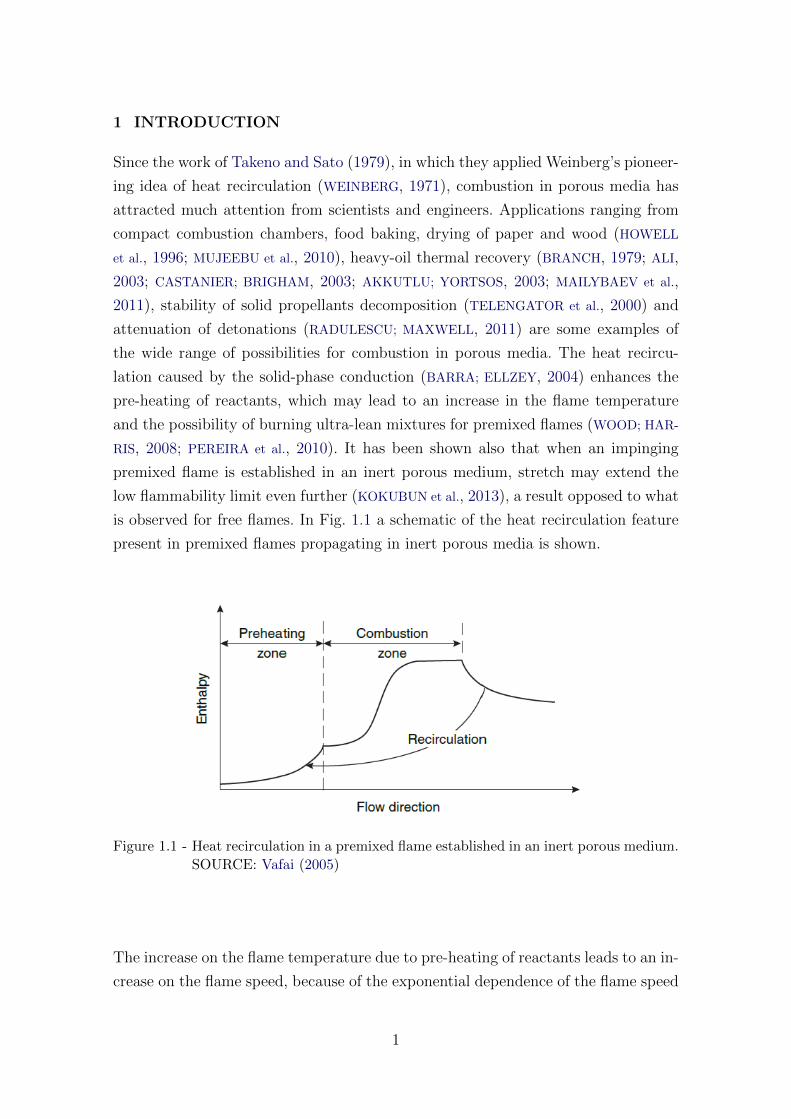
is observed for free flames. In Fig. 1.1 a schematic of the heat recirculation feature
present in premixed flames propagating in inert porous media is shown.
Figure 1.1 - Heat recirculation in a premixed flame established in an inert porous medium.
SOURCE: Vafai (2005)
The increase on the flame temperature due to pre-heating of reactants leads to an in-
crease on the flame speed, because of the exponential dependence of the flame speed
1
with the flame temperature, as flame structure analyses show (YARIN; SUKHOV, 1992;
KAKUTKINA, 2006; LAEVSKII; BABKIN, 2008; PEREIRA et al., 2009). If the constant
flame speed is different from the constant flow speed, there is a speed associated with
the heating of the solid, i.e., thermal speed. When the flame speed and the thermal
speed have the same constant value, the superadiabatic effect (flame temperature
above the adiabatic value) is maximum because these processes sustain each other.
If the problem is stationary or if the characteristic time of the thermal speed is very
short, the solid is considered to be instantaneously heated in the flame propagation
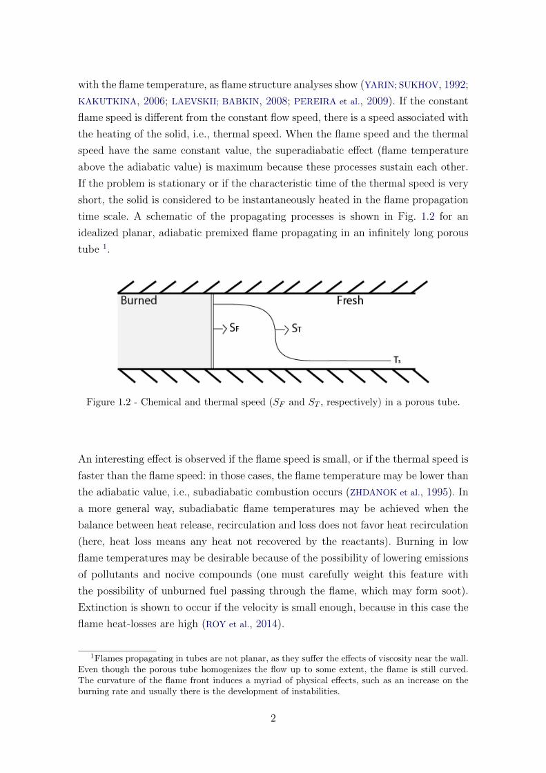
time scale. A schematic of the propagating processes is shown in Fig. 1.2 for an
idealized planar, adiabatic premixed flame propagating in an infinitely long porous
tube 1.
Figure 1.2 - Chemical and thermal speed (SF and ST , respectively) in a porous tube.
An interesting effect is observed if the flame speed is small, or if the thermal speed is
faster than the flame speed: in those cases, the flame temperature may be lower than
the adiabatic value, i.e., subadiabatic combustion occurs (ZHDANOK et al., 1995). In
a more general way, subadiabatic flame temperatures may be achieved when the
balance between heat release, recirculation and loss does not favor heat recirculation
(here, heat loss means any heat not recovered by the reactants). Burning in low
flame temperatures may be desirable because of the possibility of lowering emissions
of pollutants and nocive compounds (one must carefully weight this feature with
the possibility of unburned fuel passing through the flame, which may form soot).
Extinction is shown to occur if the velocity is small enough, because in this case the
flame heat-losses are high (ROY et al., 2014).
1Flames propagating in tubes are not planar, as they suffer the effects of viscosity near the wall.Even though the porous tube homogenizes the flow up to some extent, the flame is still curved.The curvature of the flame front induces a myriad of physical effects, such as an increase on theburning rate and usually there is the development of instabilities.
2
When it comes to nonpremixed combustion in porous media, the literature is not
vast as for premixed flames. The first attempts on modelling liquid fuel burning in
porous media focused on droplet injection inside the solid matrix (TSENG; HOWELL,
1996). For burning of liquid fuels, the intense radiation field generated by the heated
solid enhances the evaporation of fuel droplets in the confined medium. For situations
such that the droplets vaporize and mix with oxidant prior to the combustion zone
(MARTYNENKO et al., 1998; KAYAL; CHAKRAVARTY, 2005), essentially a premixed
flame is established. Liquid-fuel-fired porous burners (non-spraying) were proposed
as a way of burning liquid fuels without resorting to injection nozzles (which are
energy-consuming) (JUJGAI et al., 2002; JUJGAI; POLMART, 2003; JUGJAI; PONGSAI,
2007). Such burners have the advantage of compactness and efficiency when com-
pared to the usual spray configuration. Low emissions of pollutants are also described
for such burners.
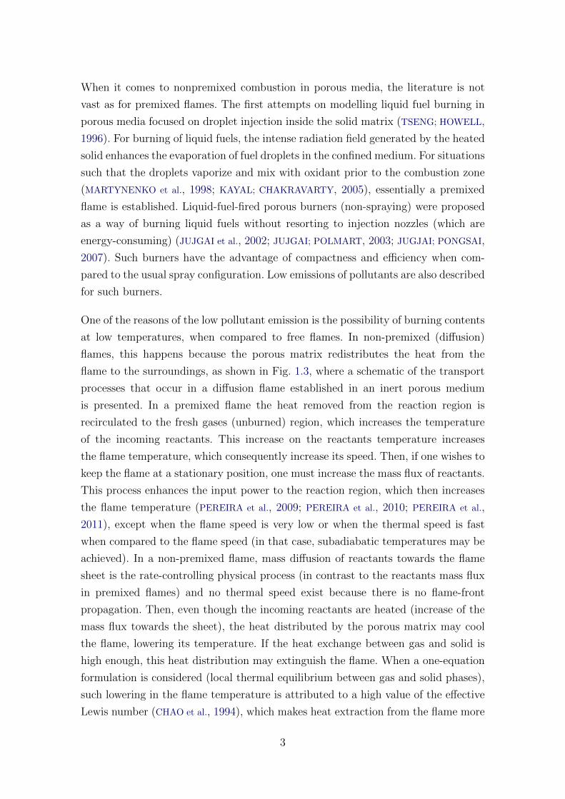
One of the reasons of the low pollutant emission is the possibility of burning contents
at low temperatures, when compared to free flames. In non-premixed (diffusion)
flames, this happens because the porous matrix redistributes the heat from the
flame to the surroundings, as shown in Fig. 1.3, where a schematic of the transport
processes that occur in a diffusion flame established in an inert porous medium
is presented. In a premixed flame the heat removed from the reaction region is
recirculated to the fresh gases (unburned) region, which increases the temperature
of the incoming reactants. This increase on the reactants temperature increases
the flame temperature, which consequently increase its speed. Then, if one wishes to
keep the flame at a stationary position, one must increase the mass flux of reactants.
This process enhances the input power to the reaction region, which then increases
the flame temperature (PEREIRA et al., 2009; PEREIRA et al., 2010; PEREIRA et al.,
2011), except when the flame speed is very low or when the thermal speed is fast
when compared to the flame speed (in that case, subadiabatic temperatures may be
achieved). In a non-premixed flame, mass diffusion of reactants towards the flame
sheet is the rate-controlling physical process (in contrast to the reactants mass flux
in premixed flames) and no thermal speed exist because there is no flame-front
propagation. Then, even though the incoming reactants are heated (increase of the
mass flux towards the sheet), the heat distributed by the porous matrix may cool
the flame, lowering its temperature. If the heat exchange between gas and solid is
high enough, this heat distribution may extinguish the flame. When a one-equation
formulation is considered (local thermal equilibrium between gas and solid phases),
such lowering in the flame temperature is attributed to a high value of the effective
Lewis number (CHAO et al., 1994), which makes heat extraction from the flame more
3
intense than mass reactants transport to the flame sheet. The effective Lewis number
is considered as the ratio between the effective thermal diffusivity and the mass
diffusivity. Since the effective thermal diffusivity is the sum of the gas and solid
thermal diffusivities, the effective Lewis number is usually high.
Figure 1.3 - Transport processes for diffusion flames established in porous media.
The difficulty in having optical access inside porous material makes it a challenge
to obtain experimental measurements. One can insert a thermocouple inside the
matrix if the porous material is carefully constructed, however, it is impossible to
distinguish between gas and solid temperature profiles because the thermocouple
will measure an average temperature. Some works have used laser measurements,
also depending on a carefully constructed porous matrix, but in these works only the
gas temperature could be measured (STELZNER et al., 2014). Indirect measurements
as combustion products emission and overall temperature profiles are usually made
(MITAL et al., 1997; JUJGAI et al., 2002; JUJGAI; POLMART, 2003; KAMAL; MOHAMAD,
2006; JUGJAI; PONGSAI, 2007) in experimental works. In this scenario, theoretical
works are important in order to better understand the confined physical processes, to
shed some light on the results that are obtained experimentally and to even provide
guidance to future experiments.
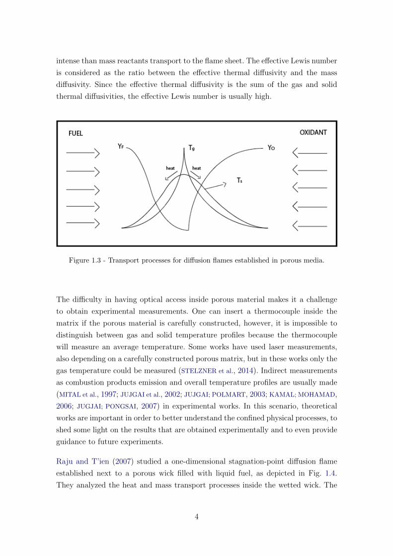
Raju and T’ien (2007) studied a one-dimensional stagnation-point diffusion flame
established next to a porous wick filled with liquid fuel, as depicted in Fig. 1.4.
They analyzed the heat and mass transport processes inside the wetted wick. The
4
diffusion flame imposes a heat flux towards the porous wick, which then is used
on the liquid-fuel phase change. Conceptually, two regimes may exist in the porous
wick: funicular, in which a two-phase vapor-liquid region exist above a purely liq-
uid region, and evaporative, in which a single phase vapor region exist, followed by
the two-phase region above the purely liquid fuel region. Intuitively, the evaporative
regime must occur for high heat fluxes. It has been shown that this regime is un-
stable (ZHAO; LIAO, 2000). Also, in their work, Raju and T’ien (2007) showed that
some fraction of liquid vapor that does not goes to combustion condensates inside
the porous wick, creating a liquid-vapor counterflow right below the wick surface.
This happens because they considered liquid ethanol. Since their focus was on the
transport processes in the two-phase region, a confined flame was not considered.
Figure 1.4 - Problem analyzed by Raju and Tien.
SOURCE: Raju and T’ien (2007)
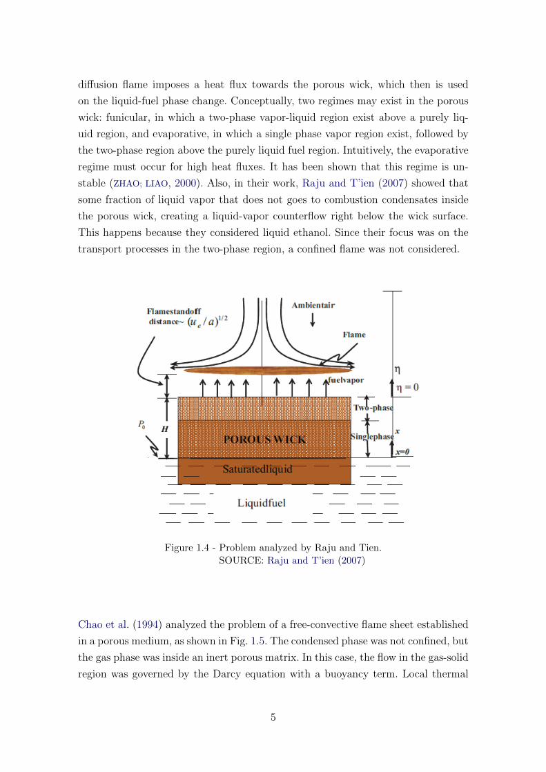
Chao et al. (1994) analyzed the problem of a free-convective flame sheet established
in a porous medium, as shown in Fig. 1.5. The condensed phase was not confined, but
the gas phase was inside an inert porous matrix. In this case, the flow in the gas-solid
region was governed by the Darcy equation with a buoyancy term. Local thermal
5
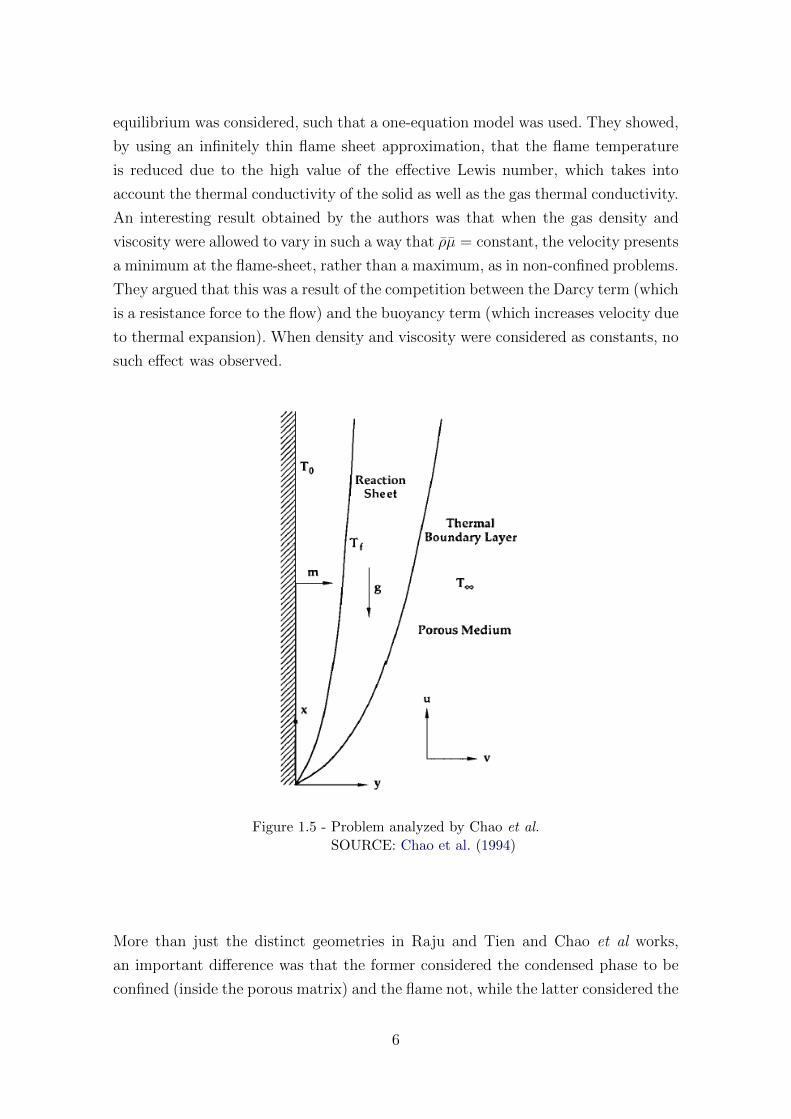
equilibrium was considered, such that a one-equation model was used. They showed,
by using an infinitely thin flame sheet approximation, that the flame temperature
is reduced due to the high value of the effective Lewis number, which takes into
account the thermal conductivity of the solid as well as the gas thermal conductivity.
An interesting result obtained by the authors was that when the gas density and
viscosity were allowed to vary in such a way that ρµ = constant, the velocity presents
a minimum at the flame-sheet, rather than a maximum, as in non-confined problems.
They argued that this was a result of the competition between the Darcy term (which
is a resistance force to the flow) and the buoyancy term (which increases velocity due
to thermal expansion). When density and viscosity were considered as constants, no
such effect was observed.
Figure 1.5 - Problem analyzed by Chao et al.
SOURCE: Chao et al. (1994)
More than just the distinct geometries in Raju and Tien and Chao et al works,
an important difference was that the former considered the condensed phase to be
confined (inside the porous matrix) and the flame not, while the latter considered the
6
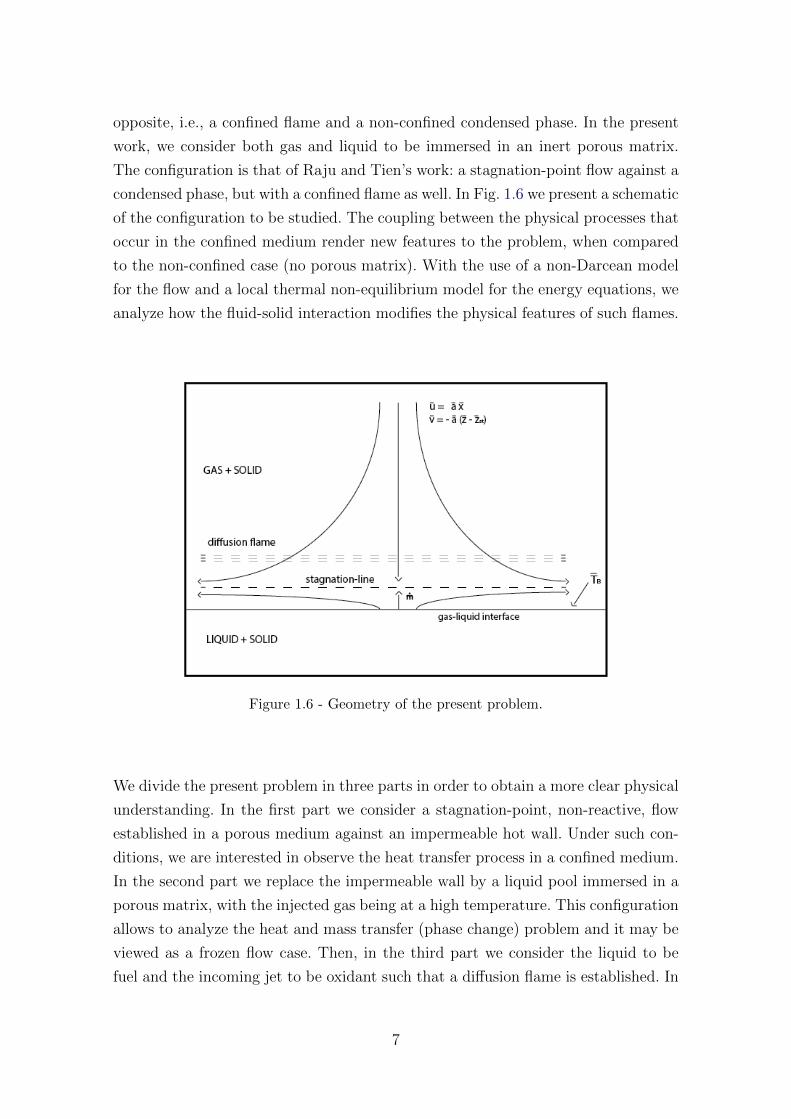
opposite, i.e., a confined flame and a non-confined condensed phase. In the present
work, we consider both gas and liquid to be immersed in an inert porous matrix.
The configuration is that of Raju and Tien’s work: a stagnation-point flow against a
condensed phase, but with a confined flame as well. In Fig. 1.6 we present a schematic
of the configuration to be studied. The coupling between the physical processes that
occur in the confined medium render new features to the problem, when compared
to the non-confined case (no porous matrix). With the use of a non-Darcean model
for the flow and a local thermal non-equilibrium model for the energy equations, we
analyze how the fluid-solid interaction modifies the physical features of such flames.
Figure 1.6 - Geometry of the present problem.
We divide the present problem in three parts in order to obtain a more clear physical
understanding. In the first part we consider a stagnation-point, non-reactive, flow
established in a porous medium against an impermeable hot wall. Under such con-
ditions, we are interested in observe the heat transfer process in a confined medium.
In the second part we replace the impermeable wall by a liquid pool immersed in a
porous matrix, with the injected gas being at a high temperature. This configuration
allows to analyze the heat and mass transfer (phase change) problem and it may be
viewed as a frozen flow case. Then, in the third part we consider the liquid to be
fuel and the incoming jet to be oxidant such that a diffusion flame is established. In
7
this third configuration we are able to study heat and mass transfer in reacting flows
inside an inert porous medium. Therefore, the division of the problem in three parts
allows for a deeper level of physical insight into the coupled processes that occur
in the presence of the inert porous matrix. In each Chapter we present a specific
introduction and physical discussion.
In the context of an incompressible flow (constant-density) and in the limit of
an asymptotically large solid-to-gas thermal conductivities ratio (defined as Γ ≡λs/λg >> 1), these three problems were analyzed previously (KOKUBUN; FACHINI,
2011; KOKUBUN; FACHINI, 2012; KOKUBUN; FACHINI, 2013). In those cases, a Darcy
flow was considered to be the leading-order flow equation and thermal equilibrium
between phases was admitted for the leading-order temperature equations. The con-
sideration of an asymptotically large Γ leads to well separated length-scales due to
the very large difference between the phases thermal conductivities. Then, in those
cases, analytical profiles were obtained in each length-scale and matched in order to
build the complete solution for each problem. Despite some minor changes in the
assumptions made, the present work can be viewed as a natural extension of these
previous works. The consideration of variables fluid properties is more realistic and
allow us to obtain a clearer picture of the physical processes that occur in these
confined problems, while the consideration of general values of Γ allow us to as-
sess more precisely the influence of the solid-to-gas thermal conductivities ratio on
the overall aspects of each problem. For instance, for the case where we consider a
stagnation-point against an impermeable wall, thermal expansion greatly modifies
wall properties, which are of interest of Engineering, such as wall shear and wall
heat flux. Consideration of thermal expansion (coupling between flow and energy
equations) and general values of Γ demands a numerical solution for the present
problem.
Since the three problems to be considered are closely related, their mathematical
formulations are similar. In the next Chapter we develop the complete mathematical
formulation (dimensional and non-dimensional) to be used in this work. Then, in
the subsequent Chapters the appropriate formulation for each problem is given and
their solutions are obtained and discussed.
In Appendix A we present an asymptotic analysis of the extinction limits of a diffu-
sion flame in a porous chamber. The geometry studied is shown in Fig. 1.7. The gen-
eral asymptotic formulation derived by Cheatham and Matalon (2000) for diffusion
flames applicable to this case is used. This analysis is made in order to clarify how
8
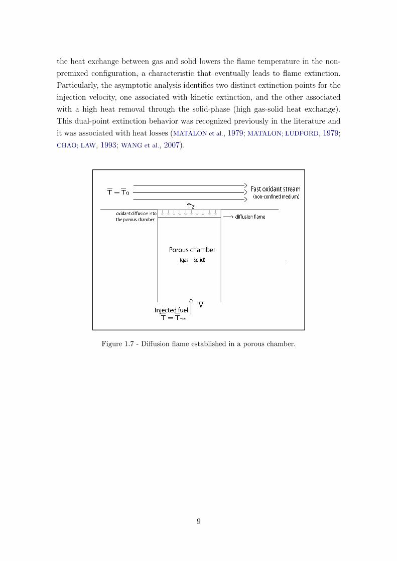
the heat exchange between gas and solid lowers the flame temperature in the non-
premixed configuration, a characteristic that eventually leads to flame extinction.
Particularly, the asymptotic analysis identifies two distinct extinction points for the
injection velocity, one associated with kinetic extinction, and the other associated
with a high heat removal through the solid-phase (high gas-solid heat exchange).
This dual-point extinction behavior was recognized previously in the literature and
it was associated with heat losses (MATALON et al., 1979; MATALON; LUDFORD, 1979;
CHAO; LAW, 1993; WANG et al., 2007).
Figure 1.7 - Diffusion flame established in a porous chamber.
9

2 MATHEMATICAL FORMULATION
In this Chapter we present the mathematical formulation to be used in this work.
The fundamental equations in the pore-scale (with the usual simplifications) are
first presented and the difficulties that arise in solving the complete problem are
exhibited. Then, the local-average procedure is briefly explained, and in the light
of such, the semi-heuristic formulation is shown. At last, the further simplifications
made in order to study the present problem are stated and the general formulation
is given.
The notation used is defined right after its first appearance. Throughout this
manuscript some symbols are repeated, but they should be clear from the context,
such that no confusion is expected.
2.1 General conservation equations and the local-average method
The conservation equations that govern the behavior of reactive flows are well-
established (WILLIAMS, 1985). In the presence of a porous matrix, these governing
equations are still valid at the pore-scale, but the energy equation in the solid phase
must be taken into account. At the interface between fluid and solid a diversity of
effects occurs, such as heat exchange, elimination of radicals, viscous attachment,
etc.
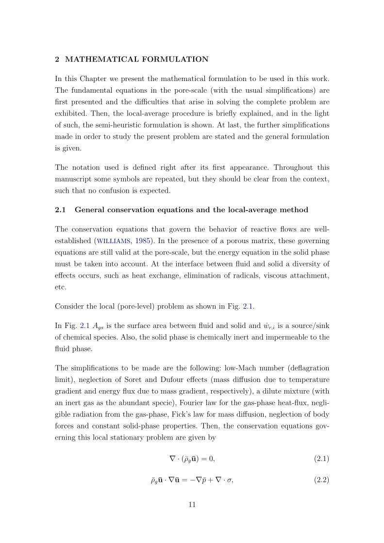
Consider the local (pore-level) problem as shown in Fig. 2.1.
In Fig. 2.1 Ags is the surface area between fluid and solid and wr,i is a source/sink
of chemical species. Also, the solid phase is chemically inert and impermeable to the
fluid phase.
The simplifications to be made are the following: low-Mach number (deflagration
limit), neglection of Soret and Dufour effects (mass diffusion due to temperature
gradient and energy flux due to mass gradient, respectively), a dilute mixture (with
an inert gas as the abundant specie), Fourier law for the gas-phase heat-flux, negli-
gible radiation from the gas-phase, Fick’s law for mass diffusion, neglection of body
forces and constant solid-phase properties. Then, the conservation equations gov-
erning this local stationary problem are given by
∇ · (ρgu) = 0, (2.1)
ρgu · ∇u = −∇p+∇ · σ, (2.2)
11
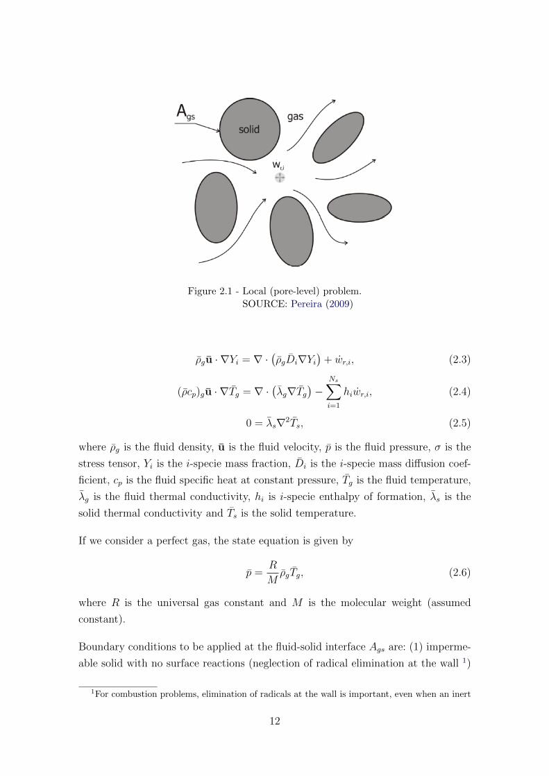
Figure 2.1 - Local (pore-level) problem.
SOURCE: Pereira (2009)
ρgu · ∇Yi = ∇ ·(ρgDi∇Yi
)+ wr,i, (2.3)
(ρcp)gu · ∇Tg = ∇ ·(λg∇Tg
)−
Ns∑i=1
hiwr,i, (2.4)
0 = λs∇2Ts, (2.5)
where ρg is the fluid density, u is the fluid velocity, p is the fluid pressure, σ is the
stress tensor, Yi is the i-specie mass fraction, Di is the i-specie mass diffusion coef-
ficient, cp is the fluid specific heat at constant pressure, Tg is the fluid temperature,
λg is the fluid thermal conductivity, hi is i-specie enthalpy of formation, λs is the
solid thermal conductivity and Ts is the solid temperature.
If we consider a perfect gas, the state equation is given by
p =R
MρgTg, (2.6)
where R is the universal gas constant and M is the molecular weight (assumed
constant).
Boundary conditions to be applied at the fluid-solid interface Ags are: (1) imperme-
able solid with no surface reactions (neglection of radical elimination at the wall 1)
1For combustion problems, elimination of radicals at the wall is important, even when an inert
12
and no-slip conditions
− ρgDi∇Yi = 0 and u = 0, (2.7)
and (2) continuity of temperature and heat flux
Tg = Ts, and λg∇Tg · ngs = (−λs∇Ts − qr,s) · ngs, (2.8)
where ngs is the unitary normal vector on Ags pointing to the solid-phase and qr,s
is the radiant heat flux at the solid surface, that is due to the radiation exchange
between solid surfaces. The equality of fluid-solid temperatures at the surface is
justified by the zero-velocity boundary condition at the pore walls.
A priori, one can solve the above set of equations and account for the solid-fluid
interaction at the pore walls. However, with the exception of the consideration of
simple geometries, this task demands an enormous computational effort. In this case,
a Direct Numerical Simulation (DNS) must be performed.
The DNS approach becomes unpractical for most cases because of the small-scale
processes imposed by the pores. Then, the method more frequently utilized is the
application of the volume averaging, in which we obtain a set of conservation equa-
tions averaged over certain representative volume containing both fluid and solid
phases. In this method, the conservation equations are averaged over some represen-
tative elementary volume (REV), or, the smallest volume that represents the local
average properties, such that addition of more pores in this volume does not change
the system properties.
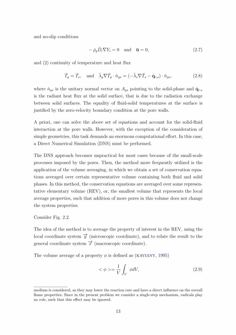
Consider Fig. 2.2.
The idea of the method is to average the property of interest in the REV, using the
local coordinate system −→y (microscopic coordinate), and to relate the result to the
general coordinate system −→x (macroscopic coordinate).
The volume average of a property φ is defined as (KAVIANY, 1995)
< φ >=1
V
∫V
φdV, (2.9)
medium is considered, as they may lower the reaction rate and have a direct influence on the overallflame properties. Since in the present problem we consider a single-step mechanism, radicals playno role, such that this effect may be ignored.
13
Figure 2.2 - Schematic of the REV approach
SOURCE: Pereira (2009)
where V is the volume of the REV. Then, the average of a gas-phase property φg
over the gas-phase volume (gas-phase intrinsic volume average) is
< φg >g=
1
Vg
∫Vg
φgdV =< φg > /ϕ. (2.10)
Where ϕ ≡ Vg/(Vg + Vs) is the porosity, or the void volume, ranging from 0 to 1.
The theorem of the intrinsic volume-averaging of the gradient of a function φg is
(KAVIANY, 1995)
< ∇φg >g= ∇ < φg >g +
1
Vg
∫Ags
φgdA. (2.11)
Analogously, the theorem of the intrinsic volume-averaging of the divergent of a
vector bg is
< ∇ · bg >g= ∇· < bg >g +
1
Vg
∫Ags
bg · ngsdA. (2.12)
One important key-point to the volume-averaging treatment is the requirement of
scales separation, which can be stated as
lp � lREV � L, (2.13)
in which lp is the pore characteristic length scale, lREV is the REV characteristic
14
length scale and L is the largest characteristic scale of the problem. Also, phe-
nomenological scales have to be separated as well. For example, for conductive heat
transfer, it is required that
∆Tlp � ∆TlREV� ∆TL, (2.14)
where ∆T represents the maximum temperature difference across the respective
length-scale. This condition represents a severe limitation to the volume-averaging
modelling of combustion in porous media. It is usually not possible to define a REV
that fulfills the separation of scales requirement since flames are characterized by a
narrow region where the fuel is consumed and the chemical energy is released (the
flame thickness) that is often of the order of a fraction of the length-scale of a single
pore.
However, despite of this limitation, with these theorems one can proceed to evaluate
the averaged conservation equations. This lengthy process is not to be reproduced
here, as it is not our focus. Relevant works are given by Kaviany (1995), Vafai (2005),
Duval et al. (2004) and Whitaker (1996).
From the theorems, it is easy to see that several terms will appear from the area
integrals. These terms can be grouped into coefficients that are to be obtained from
DNS calculations or experimental correlations. For instance, the volume-averaged
gas-phase energy equation is given by
vgg · ∇ < Tg >g +vgs · ∇ < Ts >
s= ∇ ·Dgg · ∇ < Tg >g +
∇.Dgs · ∇ < Ts >s +
AgsVg
hc(ρcp)g
(< Ts >
s − < Tg >g)
+ < sr >g, (2.15)
where the convective velocity vectors vgg and vgs are the coefficients of the terms
containing the first-order derivatives, the total thermal diffusivity tensors Dgg and
Dgs are the coefficients of the terms containing second-order derivatives, hc is the
interfacial conduction heat transfer coefficient, that is independent from the fluid
velocity, and < sr >g is an energy source term.
The derivation of the volume-averaged momentum conservation equation in a form
equivalent to the Navier-Stokes equation is still an open problem. Some simplified
forms are proposed in the literature (KAVIANY, 1995).
Since the conservation equations obtained from the volume-averaging procedure still
depends on DNS calculations or experimental correlations and are quite compli-
15
cated, it is common to resort to a semi-heuristic approach. In this approach, the
conservation equations take into account the fluid-solid interaction through phys-
ical arguments, but can not be obtained from the first principles. Although less
complete, this semi-heuristic approach is useful in capturing the relevant physical
aspects of the fluid-solid interaction. For instance, the superadiabatic temperatures
achieved in combustion in porous media have been reproduced with the aid of such
semi-heuristic formulation (PEREIRA et al., 2009; PEREIRA et al., 2010; PEREIRA et al.,
2011; KOKUBUN et al., 2013). Such superadiabatic temperatures enhance the flamma-
bility limit of premixed flames, allowing burning of ultra-lean mixtures (WOOD; HAR-
RIS, 2008). In opposition to the superadiabtic flames, so-called subadiabatic flames
have been predicted theoretically (MIN; SHIN, 1991) and later obtained experimen-
tally (VOGEL; ELLZEY, 2005). Low flame temperatures in the diffusion-flame regime
were also predicted theoretically with the use of a simple semi-heuristic formulation
(CHAO et al., 1994). Burning in low flame temperatures is an useful feature in low-
ering emissions of pollutants and formation of hazardous compounds, like NOx, for
instance (JUGJAI; PONGSAI, 2007; JUGJAI; PHOTHIYA, 2007).
2.2 Semi-heuristic formulation
The semi-heuristic equations of mass, mass fractions and energies are given by
∇ · ρgu = 0, (2.16)
ρgu · ∇Yi = ϕ∇ · (ρgDi · ∇Yi)− ϕwr,i, (2.17)
ρgcp,gu · ∇Tg = ϕ∇ ·(λg · ∇Tg
)+ hg
(Ts − Tg
)+ ϕwr,i, (2.18)
0 = (1− ϕ)∇ ·(λs · ∇Ts
)− hg
(Ts − Tg
)+∇ · qr, (2.19)
in which Di is the mass diffusivity tensor of specie i, which contains mass disper-
sion effects, λg is the thermal conductivity tensor of the gas-phase, which contains
thermal dispersion effects, qr is the radiant heat flux vector and hg is the volumetric
interphase heat exchange coefficient.
For simplicity, it is usual to model the reaction source term as measured with its
averaged properties. Hence, for a single-step, second order reaction-rate, we have
wr,F = Bρ2gT
ag YF YO exp
(− EaRTg
), (2.20)
where Ea is the activation energy, B is the frequency factor and a is a constant (that
16
will be taken as a = 1 in Chapters 2 and 5, and as a = 0 in Appendix A).
The semi-heuristic momentum conservation equation is written as
ρgu · ∇u = −ϕ∇p+∇ (µ∇u)− ϕ µK
u− ϕ CE
K1/2ρg|u|u, (2.21)
where K is the permeability tensor and CE is the Ergun constant. The left-hand side
are the macroscopic inertia forces. The first term in the right-hand-side is the pore
pressure gradient, the second term is the macroscopic shear stress diffusion term
(Brinkman viscous term), the third term is the microscopic viscous shear stress
(Darcy term) and the fourth term is the microscopic inertial force term (Ergun
inertial term).
For closure, the ideal gas equation of state is given by
p =R
MρgTg. (2.22)
This set of equations is simpler than that obtained from the rigorous application
of the volume average method to the local problem. Here, the effects of the many
coefficients that appear in the original equations are accounted for using fewer coef-
ficients, namely the thermal conductivity tensors of both phases, the mass diffusion
tensor and the superficial convection heat transfer coefficient. For the momentum
conservation equation, the resistance force due to the tortuous porous channels is
accounted through the last two terms in Eq. 2.21.
2.3 Formulation for the present work
In the present work we consider a stagnation-point flow of oxidant against a pool
of liquid fuel, with the whole system immersed in an inert porous medium. In the
region where the mass fluxes are nearly in a stoichiometric proportion, a diffusion
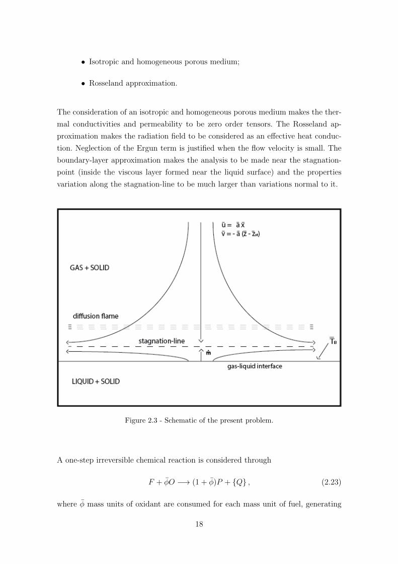
flame is established. A schematic of the problem is shown in Fig. 2.3.
To solve this problem we consider some additional simplifications in order to obtain
the set of equations to be used. These simplifications are
• Two-dimensional problem;
• Boundary-layer approximation;
• Neglect of the Ergun term;
17
• Isotropic and homogeneous porous medium;
• Rosseland approximation.
The consideration of an isotropic and homogeneous porous medium makes the ther-
mal conductivities and permeability to be zero order tensors. The Rosseland ap-
proximation makes the radiation field to be considered as an effective heat conduc-
tion. Neglection of the Ergun term is justified when the flow velocity is small. The
boundary-layer approximation makes the analysis to be made near the stagnation-
point (inside the viscous layer formed near the liquid surface) and the properties
variation along the stagnation-line to be much larger than variations normal to it.
Figure 2.3 - Schematic of the present problem.
A one-step irreversible chemical reaction is considered through
F + φO −→ (1 + φ)P + {Q} , (2.23)
where φ mass units of oxidant are consumed for each mass unit of fuel, generating
18
(1 + φ) mass units of product and releasing an amount Q of heat.
The two spatial coordinates are x (tangential to the liquid surface) and z (normal
to the liquid surface). Below z = 0 the porous matrix is filled with liquid fuel.
For z > 0 we have a pure gas flow and the conservation equations, with the simpli-
fications stated previously, are given by
ρ∂u
∂x+∂ρv
∂z= 0, (2.24)
ρu∂u
∂x+ ρv
∂u
∂z= −ϕ∂p
∂x+
∂
∂z
(µ∂u
∂z
)− ϕµ u
K, (2.25)
ρu∂v
∂x+ ρv
∂v
∂z= −ϕ∂p
∂z+
∂
∂z
(µ∂v
∂z
)− ϕµ v
K, (2.26)
ρvdYFdz− ϕ d
dz
(ρDF
dYFdz
)= −ϕBρ2TgYF Y0e
−Ea/RTg , (2.27)
ρvdYOdz− ϕ d
dz
(ρDO
dYOdz
)= −ϕφBρ2TgYF Y0e
−Ea/RTg , (2.28)
ρvcpdTgdz− ϕ d
dz
(λgdTgdz
)= ϕQBρ2TgYF Y0e
−Ea/RTg + hg(Ts − Tg), (2.29)
− (1− ϕ)λsd2Tsdz2
= −hg(Ts − Tg
), (2.30)
where u and v are the Darcy velocities, related with the local velocities ulo and vlo
through {u, v} = ϕ {ulo, vlo}, where ϕ is the porosity.
The relation between the permeability K and the porosity ϕ depends on the model
utilized for the porous matrix. In the present work we consider a bed of particles, or
fibers, which gives the permeability K as (KAVIANY, 1995)
K =d2p
180
ϕ3
(1− ϕ)2, (2.31)
where dp is the mean particle diameter.
For simplicity, we consider the liquid fuel to be at its boiling temperature, such that
Tl = TB and the only equations needed in the liquid-solid region, z < 0, are the
mass conservation and the solid energy equation, given by
ρlvl = ¯m, (2.32)
19
− (1− ϕ)λsd2Tsdz2
= −hl(Ts − TB). (2.33)
For z → +∞ (far from the viscous boundary-layer) the flow is potential-like, gas
and solid phases are at thermal equilibrium and only oxidant is observed. Those
conditions are expressed as
u = ax, v = −a(z − zst), Tg = Ts = T∞, YO = YO∞, YF = 0, (2.34)
in which a is the strain-rate and zst is the position of the stagnation-point (which is
determined by the vaporization rate ¯m).
The boundary conditions for the liquid-fuel reservoir, z → −∞, are given by
vl = vl−∞, Ts = TB. (2.35)
The injection velocity vl−∞ is such that the interface remains fixed at z = 0.
At the liquid-gas interface, z = 0, we consider ρ/ρl � 1 such that the no-slip
condition u = 0 may be used, as shown previously (SESHADRI et al., 2008). The
vertical velocity v(0) is an unknown related with the vaporization rate ¯m. We assume
that gas and liquid are at equilibrium at the interface, such that Tg(0+) = TB. The
solid conducts heat from the gas-solid region and at the interface it is at a higher
temperature than the gas, at Ts(0) > TB.
Since the liquid is at its boiling temperature and the solid temperature is higher
(Ts(0) > TB), below the gas-liquid interface there is a three-phase (liquid-gas-solid)
region with a high heat flux from above imposed by the flame sheet. Zhao and Liao
(2000) have shown that for low heat flux, the evaporation process occurs uniformly
at the surface. For increasing heat fluxes, a three-phase region is observed below
the surface. This three-phase region is characterized by the appearance of gaseous
bubbles at the pore walls, which decreases the effective heat transfer from solid to
liquid. A schematic of the bubble formation in the three-phase region, when the heat
flux is high, is shown in Fig. 2.4.
Modeling this three-phase region is quite complicated, with the need of considering
the interaction between gas, liquid and solid in this zone (RAJU; T’IEN, 2007). Since
our focus is mainly on how the porous medium affect the flame, when compared
to the non-confined case, a detailed model of this three-phase region is not needed.
For our purposes it is enough to model this phase-change region, denoted as boiling
20
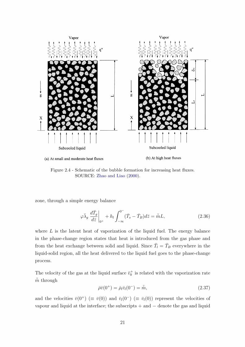
Figure 2.4 - Schematic of the bubble formation for increasing heat fluxes.
SOURCE: Zhao and Liao (2000).
zone, through a simple energy balance
ϕλgdTgdz
∣∣∣∣0+
+ hl
∫ 0−
−∞(Ts − TB)dz = ¯mL, (2.36)
where L is the latent heat of vaporization of the liquid fuel. The energy balance
in the phase-change region states that heat is introduced from the gas phase and
from the heat exchange between solid and liquid. Since Tl = TB everywhere in the
liquid-solid region, all the heat delivered to the liquid fuel goes to the phase-change
process.
The velocity of the gas at the liquid surface v+0 is related with the vaporization rate
¯m through
ρv(0+) = ρlvl(0−) = ¯m, (2.37)
and the velocities v(0+) (≡ v(0)) and vl(0−) (≡ vl(0)) represent the velocities of
vapour and liquid at the interface; the subscripts + and − denote the gas and liquid
21
sides of the interface, respectively.
At the interface, integration of Eq. 2.27 gives the fuel mass fraction conservation as
ϕρDFdYFdz
∣∣∣∣0+
= −(1− YF0
)(ρv)|0+ . (2.38)
For closure of the problem, we have the state equation
p = ρRTg. (2.39)
2.3.1 Variable change and non-dimensional formulation
The non-dimensional variables are defined as u ≡ u/vc, v ≡ v/vc, p ≡ p/(ρ∞v2c ),
ρ ≡ ρ/ρ∞, ρl ≡ ρl/ρ∞, x ≡ x/lc, z ≡ z/lc, Tg ≡ Tg/T∞, Ts ≡ Ts/T∞, Tl ≡ Tl/T∞
and YO ≡ YO/YO∞, YF ≡ YF , in which vc ≡ a lc is a characteristic velocity of
the problem related with the characteristic length scale lc ≡ λg∞/(ρ∞cpvc). The
characteristic length scale lc is then given by lc =√λg∞/(ρ∞cpa).
For z → +∞, momentum equations with 2.34 give the pressure distribution as
p0 − p =ρ∞a
2
2ϕ
[x2 + (z − zst)2]+
aµ∞2K
[x2 − (z − zst)2] . (2.40)
For the limit ϕ→ 1 we recover the usual pressure distribution for the non-confined
stagnation-point flow (SCHLICHTING, 1968). From the model used for the perme-
ability, Eq. 2.31, ϕ → 1 leads to K → ∞. The second term in the right-hand side
of the expression 2.40 is the modification on the pressure distribution due to the
presence of the porous matrix. Note that the lower the medium permeability, the
higher the influence of the porous medium on the pressure field.
We introduce the following transformed variables in the gas-solid region
u = xU(η), ρv = −f(η), η =
∫ρdz,
p0 − p =1
2ϕ
[x2 + 2F (η)
]+Pr
2K
[x2 − 2F (η)
], (2.41)
where Pr is the Prandtl number, assumed constant, K ≡ K/l2c is the non-
dimensional permeability (Darcy number) and η is a mass-weighted coordinate. We
consider a temperature dependence of the viscosity, gas-phase thermal conductivity
22
and mass diffusion such that ρµ/µ∞ = ρλg/λg∞ = ρ2Di/Di∞ = 1. This temperature-
dependence was chosen to simplify the analysis, but extension to more realistic de-
pendences can be easily considered. The first two variable transformations in 2.41
satisfies the mass conservation equation through U = df/dη.
Non-dimensional governing equations are then given by
Prd3f
dη3+ f
d2f
dη2−(df
dη
)2
− βT 2g
df
dη= −Tg (1 + β) , (2.42)
Prd2(fTg)
dη2+ f
d(fTg)
dη− βT 3
g f = (1− β)dF
dη, (2.43)
− f dYFdη− ϕ
LF
d2YFdη2
= −ϕDaYFYOe−Ta/Tg , (2.44)
− f dYOdη− ϕ
LO
d2YOdη2
= −ϕφDaYFYOe−Ta/Tg , (2.45)
− f dTgdη− ϕd
2Tgdη2
= ϕqDaYFYOe−Ta/Tg + TgNg (Ts − Tg) , (2.46)
− Γ(1− ϕ)d
dη
(1
Tg
dTsdη
)= −TgNg (Ts − Tg) , (2.47)
where we defined Ng ≡ hg/(ρ∞cpa), β ≡ ϕPr/K (inversely proportional to the
Darcy number), Γ ≡ λs/λg∞, Da ≡ AYO∞pc/(aR) (Damkohler number, where pc
is some characteristic pressure), Ta ≡ Ea/(RT∞), φ ≡ φ/YO∞, q ≡ Q/(cpT∞) and
if we assume that the average molecular weight is constant in our domain, we have
ρ = 1/Tg, i.e., variations in pressure are higher-order.
Since we consider Tl = TB everywhere in the liquid region, the only equation needed
is the solid energy equation, which is given by
− Γ(1− ϕ)d2Tsdz2
= −Nl(Ts − TB), (2.48)
where Nl ≡ hl/(ρ∞cpa). Note that in the liquid-solid region the spatial coordinate
is only made non-dimensional. This is because the flow in the liquid-solid region is
trivial.
Boundary conditions for η →∞ become
df
dη= 1, Ts = Tg = 1, YF = 0, YO = 1. (2.49)
23
At the surface η = 0, we have
df
dη= 0, Tg = TB, YO = 0. (2.50)
The relation between velocities at the interface and the liquid mass conservation
gives
− f(0) = m, (2.51)
where m ≡ ¯m/(ρ∞√aαg) is the vaporization rate, which determines the mass flux
f(0) at the interface η = 0+. The solid temperature at the surface Ts(0) > TB is
an unknown to be obtained from the continuity of the solid phase heat flux at the
gas-liquid interface, given by
1
TB
dTsdη
∣∣∣∣0+
=dTsdz
∣∣∣∣0−. (2.52)
The term 1/TB appears in the left-hand side of the above equality because of the
use of different spatial coordinates in the gas-solid and in the liquid-solid regions.
Note that TB = Tg(0).
Reservoir condition, z → −∞, is given by
Ts = TB. (2.53)
At the interface η = z = 0, fuel mass fraction and energy conservation gives
ϕ
LF
dYFdη
∣∣∣∣0
= (1− YF0)f(0), (2.54)
ϕdTgdη
∣∣∣∣0+
+Nl
∫ 0−
−∞(Ts − TB)dz = m l TB, (2.55)
where l ≡ L/(cpTB) is the dimensionless latent heat of vaporization. The effective
latent heat is given by l TB because we define l with TB instead of T∞. Species
conservation at the interface 2.54 determines YF0, while energy conservation 2.55
determines the vaporization rate m.
From the definition of β and the model used for K we have
β = 180
(δ2
d2p
)(1− ϕϕ
)2
, (2.56)
24
where δ =√ν/a is the thickness of the macroscopic viscous boundary-layer, with
ν = µ∞/ρ∞ the gas kinematic viscosity far from the boundary-layer. Hence, β is
proportional to the square of the ratio between the thickness of the macroscopic
viscous boundary-layer δ and the mean particle diameter dp and to the square of the
ratio between the solid phase volume (1−ϕ) and the gas phase volume ϕ. With some
modifications, this discussion for β was made by Wu et al. (2005), who also showed
that for low enough permeability (high enough β), convective effects are negligible
and in this case the flow is determined by a balance between the Darcy pressure
term and viscous effect. For simplification, we define β∗ ≡ 180δ2/d2p, which results
in β = β∗[(1− ϕ)/ϕ]2. Then, β varies with the porosity, but β∗ no.
If β � 1, then the flow is leading-order governed by the Darcy equation (modified
in order to account for thermal expansion). On the other hand, if β � 1, then
the Darcy term is a correction to the flow. In the energy conservation equations, if
Ng � 1, then leading-order thermal equilibrium between gas and solid is observed.
In this case, thermal non-equilibrium will be restricted to small regions near the
gas-liquid surface and around the flame sheet. If Ng � 1, then gas and solid phases
have a weak thermal coupling. The same discussion is valid for Nl.
From the momentum equation, Eq. 2.43, we can see that β = 1 represents a turning
point for the pressure distribution. For β > 1 we observe a maximum pressure above
the stagnation-point, while for β < 1 the maximum pressure is at the stagnation-
point, as in a non-confined problem. This feature was discussed previously (WU et
al., 2005) and the explanation was that for β > 1 the fiber-level viscous dissipation
was high, such that a higher pressure could be achieved above the stagnation-point.
When β = 1, Eq. 2.41 shows that p0 − p = ϕx2 (1 + β) /2. Particularly, at x = 0,
p = p0, which shows that no flow would occur for β = 1, as the pressure is constant
along the stagnation-line. By examining Eq. 2.43 we see that β = 1 is a singular
point. Hence, we do not consider it in our calculations. This result suggest that the
model may not be valid for β ≥ 1.
The term 1/Tg in the left-hand side of Eq. 2.47 appears from the coordinate trans-
formation η =∫ρdz. Then, this transformation leads to an effective solid thermal
conductivity Γ(1−ϕ)/Tg in the η plane. When Tg < 1, the solid has a larger effective
thermal conductivity in the transformed coordinate η, while the opposite holds when
Tg > 1. This happens because η is a mass-weighted coordinate, and when Tg > 1,
from the state equation ρ = 1/Tg, η < z, while for Tg < 1, η > z. Then, in order
to correctly account for the solid thermal conductivity, a correction must be made
25
for the solid energy equation in the η plane. Far enough from the surface, when
Tg ∼ 1, η ∼ z, such that the solid thermal conductivity in the η plane is equal to
the conductivity on the physical z plane.
The term Tg in the right-hand side of Eqs. 2.46 and 2.47 is also a consequence of
the coordinate transformation. When η > z (Tg < 1), the flow residence time in
the η plane is greater than in the physical z plane, increasing the interphase heat
exchange. The opposite holds when η < z (Tg > 1). In order to correctly account for
the heat exchange term, the Tg appears in the governing equations in the η plane.
2.3.2 Numerical method
In order to numerically solve the set of conservation equations, we use a finite-
difference method with a pseudo-time marching technique. We first guess initial
profiles that satisfies the boundary conditions and then add a fictitious unsteady
term to the equations and the steady-state solution is obtained by marching in the
pseudo-time (we use an explicit method for the pseudo-time derivatives). Conver-
gence is said to be achieved when the transient terms ∂/∂t are less than 10−5. We
solve the flow for U = df/dη and then obtain f by integrating the solution for U
(T’IEN et al., 1978). The conservation equation for U is second-order, then easily
integrated.
For the first problem (Hiemenz flow), a higher-order central difference scheme is
used for the first derivatives, such that the error ∼ ∆η2, where ∆η is the constant
mesh spacing. For the two remaining problems (vaporization and combustion), an
upwind scheme is used for the convective terms, such that care must be taken when
f < 0. The free stream is considered to be achieved when dTs/dη ∼ 10−4, i.e., there
is no heat flux to outside the domain.
The constant mesh spacing for the first two problems is considered as ∆η = 0.05,
while for the third part we consider ∆η = 2.5× 10⁻². For the first part we compare
our results (with the appropriate parameters) with the results obtained by Howarth
(1938), and it was shown that ∆η = 0.05 gives an error of less than 1%. For the
second and third part, the constant mesh spacing was such that lowering this value
in half showed no significant variation in the vaporization rate (burning rate) −f(0).
2.4 Physical discussion
The interaction between gas, liquid and solid renders complexities to the problem.
The tortuous channels of the porous matrix imposes a resistive force to the flow.
26
This resistance force imposed to the flow by the porous matrix is accounted through
the parameter β in Eqs. 2.42 and 2.43. Thermal expansion of the gas increases the
gas velocity, which increases the Darcy resistance force. This feature is accounted
through the term T 2g in Eq. 2.42. When ϕ → 1, β → 0 and if N → 0 the usual
reactive boundary-layer equations for the non-confined stagnation-point flow are
recovered.
If β � 1, the flow is leading-order given by the Darcy equation (modified in order to
account for thermal expansion). For the model used for K, the limit of β � 1 can be
achieved for low porosities - see Eq. 2.56. In this case, a high pressure gradient must
be imposed in order establish a flow due to the low value of the medium permeability
(recall that β ∼ 1/K). Then, when β � 1, high hydraulic losses are expected. Also,
when the pores are large, the Rosseland approximation is no longer valid and in this
case one must consider heat transport through radiation by the solid phase.
In the energy equations, the coupling is given by the heat exchange between phases
(right-hand side of Eqs. 2.46 and 2.47). When a heat source is present (in the present
case, such heat source is the flame), considering the local thermal non-equilibrium
between phases is essential. Heat is released at the flame sheet by the exothermic
reaction and is conducted away from the sheet by the gas, which then exchanges it
with the solid. Since the solid has a higher thermal conductivity, when compared to
the gas, the heat is transported to large regions from the flame sheet, and in the
process, it heats the incoming reactants. However, as discussed in the previous Sec-
tion, the heat distribution by the solid matrix cools the flame, as the rate-controlling
process for this flame is mass diffusion, rather than mass flux as in premixed flames.
27

3 HEAT AND MOMENTUM TRANSFER PROBLEM:
STAGNATION-POINT FLOW AGAINST AN IMPERMEABLE
WALL
In this Chapter we analyze a stagnation-point flow established in an inert porous
medium with heat exchange. We consider an impinging jet against an impermeable
hot wall. Then, only the frozen equations for η > 0 are necessary (Eqs. 2.42, 2.43,
2.46 and 2.47), such that the reaction term in the gas energy equation is set to
zero. Liquid equations are not necessary. The equations for YF and YO are neglected
(YF does not exist in this case, and the equation for YO does not add any relevant
information).
The influence of the wall temperature T0, porosity ϕ, gas-solid heat exchange Ng
and solid-to-gas thermal conductivities ratio Γ on the wall properties and profiles
is analyzed. The results presented here have applications on the context of heat
exchangers.
Porous media that have a higher permeability whilst having a large thermal conduc-
tivity (compared to the gas thermal conductivity), are widely used as heat exchang-
ers as they increase heat dissipation (VAFAI; KIM, 1990; JENG; TZENG, 2007). This
enhancement occurs due to the heat conduction through the solid phase and the gas-
solid heat exchange. While the majority of heat transfer problems in porous media
consider local thermal equilibrium, such that a single energy conservation equation
is used, porous heat exchangers must be analyzed with the use of the two-equation
formulation: gas and solid are at thermal non-equilibrium. The local thermal non-
equilibrium feature is essential in determining the characteristics and to assess the
efficiency of heat exchangers.
When a non-isothermal problem is considered, heat and momentum transfer are
coupled. If a constant-density model is used, the temperature field is obtained a
posteriori from the flow field. Attia (2007) studied the effect of the porosity in a
stagnation-point flow impinging on a permeable surface by using a porosity param-
eter (inversely proportional to the porosity). At the impermeable wall, suction or
injection could be admitted as the boundary condition for the velocity. Results in-
dicated that increasing the porosity parameter, i.e., reducing the medium porosity,
causes a decrease on the thickness of both thermal and velocity boundary-layers and
an increase in the heat transfer at the permeable surface.
For simple geometries and flows, analytical solutions may be obtained. Lee and
29
Vafai (1999) provided an extensive analytical characterization of forced convective
flow through a channel filled with a porous material. A heated wall was considered
to provide heat flux transversely to the flow. They obtained exact solutions for the
transverse temperature profiles of solid and fluid phases, and classified heat transfer
characteristics into three regimes, each of them dominated by a different physical
heat transfer mechanism: fluid conduction, solid conduction and internal heat ex-
change between solid and fluid phases. Based on the results obtained, a complete
electrical thermal network representative of transport through porous media was
established.
Kokubun and Fachini (2011) analyzed a stagnation-point flow in a porous medium
against an impermeable wall with heat exchange with a constant-density model,
and hence, obtained analytical solutions for the profiles. The asymptotic limit of
Γ ≡ λs/λg >> 1 (large solid-to-gas thermal conductivities ratio) was considered.
In that limit, two regions of interest exist: a large, outer region, in which the flow
is potential and an inner region, near-wall, where viscous effect balance the Darcy
pressure term. The interphase heat exchange was considered of the order of Γ, i.e.,
very large, such that in the outer region thermal equilibrium was admitted, with
thermal non-equilibrium being observed only in the inner region.
For non-isothermal problems the constant-density assumption is not realistic. The
deviations in the density field modifies the flow field, which may result in errors in
the calculation of the parameters of interest, such as the wall heat transfer and the
wall shear. The disparity between gas and solid thermal conductivities also adds
complexity to the problem, as heat transfer may occur in different length scales for
each phase, as discussed previously (KOKUBUN; FACHINI, 2011).
Here, we extend the previous results (KOKUBUN; FACHINI, 2011) by allowing gas
thermal expansion (variable density) and general values of Γ. Hence, a numerical
solution is sought to the coupled heat and momentum transfer problem.
3.1 Physical problem
The geometry to be studied is a two-dimensional stagnation-point flow established
in an inert porous medium against an impermeable wall at a constant temperature
T0, higher than T∞ (temperature of the incoming jet). Due to the hot wall, ther-
mal expansion decreases the gas density and couples flow and energy equations. A
schematic of the problem is shown in Fig. 3.1, where x is the spatial coordinate tan-
gential to the impermeable wall and z is the normal coordinate. The impermeable
30
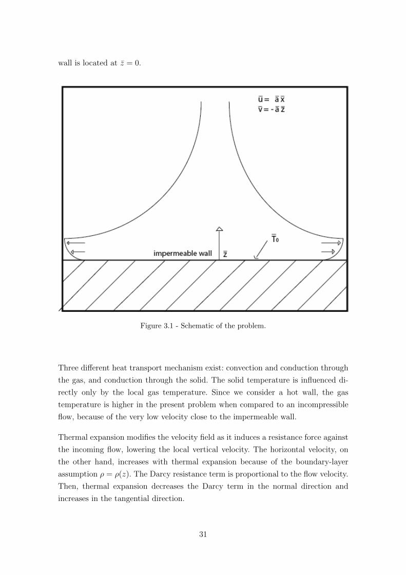
wall is located at z = 0.
Figure 3.1 - Schematic of the problem.
Three different heat transport mechanism exist: convection and conduction through
the gas, and conduction through the solid. The solid temperature is influenced di-
rectly only by the local gas temperature. Since we consider a hot wall, the gas
temperature is higher in the present problem when compared to an incompressible
flow, because of the very low velocity close to the impermeable wall.
Thermal expansion modifies the velocity field as it induces a resistance force against
the incoming flow, lowering the local vertical velocity. The horizontal velocity, on
the other hand, increases with thermal expansion because of the boundary-layer
assumption ρ = ρ(z). The Darcy resistance term is proportional to the flow velocity.
Then, thermal expansion decreases the Darcy term in the normal direction and
increases in the tangential direction.
31
3.2 Mathematical formulation
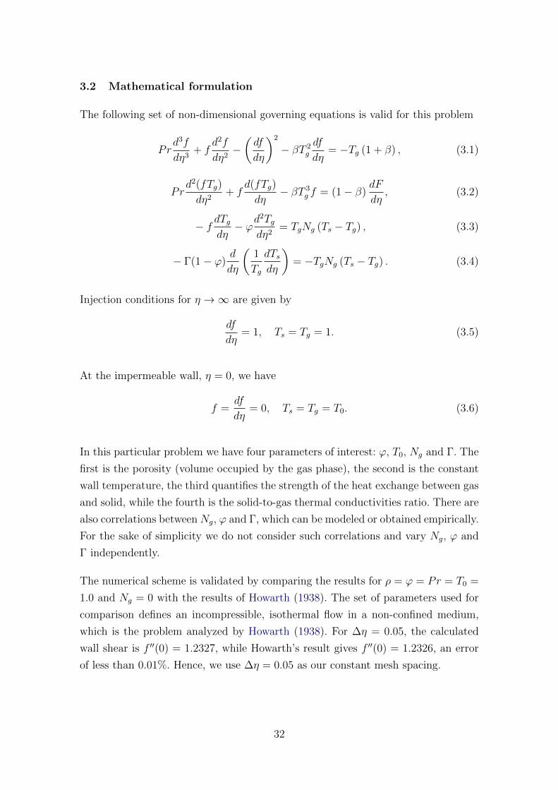
The following set of non-dimensional governing equations is valid for this problem
Prd3f
dη3+ f
d2f
dη2−(df
dη
)2
− βT 2g
df
dη= −Tg (1 + β) , (3.1)
Prd2(fTg)
dη2+ f
d(fTg)
dη− βT 3
g f = (1− β)dF
dη, (3.2)
− f dTgdη− ϕd
2Tgdη2
= TgNg (Ts − Tg) , (3.3)
− Γ(1− ϕ)d
dη
(1
Tg
dTsdη
)= −TgNg (Ts − Tg) . (3.4)
Injection conditions for η →∞ are given by
df
dη= 1, Ts = Tg = 1. (3.5)
At the impermeable wall, η = 0, we have
f =df
dη= 0, Ts = Tg = T0. (3.6)
In this particular problem we have four parameters of interest: ϕ, T0, Ng and Γ. The
first is the porosity (volume occupied by the gas phase), the second is the constant
wall temperature, the third quantifies the strength of the heat exchange between gas
and solid, while the fourth is the solid-to-gas thermal conductivities ratio. There are
also correlations between Ng, ϕ and Γ, which can be modeled or obtained empirically.
For the sake of simplicity we do not consider such correlations and vary Ng, ϕ and
Γ independently.
The numerical scheme is validated by comparing the results for ρ = ϕ = Pr = T0 =
1.0 and Ng = 0 with the results of Howarth (1938). The set of parameters used for
comparison defines an incompressible, isothermal flow in a non-confined medium,
which is the problem analyzed by Howarth (1938). For ∆η = 0.05, the calculated
wall shear is f ′′(0) = 1.2327, while Howarth’s result gives f ′′(0) = 1.2326, an error
of less than 0.01%. Hence, we use ∆η = 0.05 as our constant mesh spacing.
32
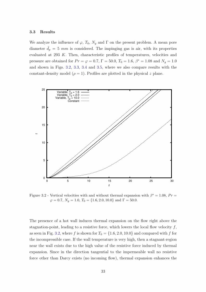
3.3 Results
We analyze the influence of ϕ, T0, Ng and Γ on the present problem. A mean pore
diameter dp = 5 mm is considered. The impinging gas is air, with its properties
evaluated at 293 K. Then, characteristic profiles of temperatures, velocities and
pressure are obtained for Pr = ϕ = 0.7, Γ = 50.0, T0 = 1.6, β∗ = 1.08 and Ng = 1.0
and shown in Figs. 3.2, 3.3, 3.4 and 3.5, where we also compare results with the
constant-density model (ρ = 1). Profiles are plotted in the physical z plane.
0
5
10
15
20
25
0 5 10 15 20 25 30
f
z
Variable, T0 = 1.6Variable, T0 = 2.0
Variable, T0 = 10.0Constant
Figure 3.2 - Vertical velocities with and without thermal expansion with β∗ = 1.08, Pr =ϕ = 0.7, Ng = 1.0, T0 = {1.6, 2.0, 10.0} and Γ = 50.0.
The presence of a hot wall induces thermal expansion on the flow right above the
stagnation-point, leading to a resistive force, which lowers the local flow velocity f ,
as seen in Fig. 3.2, where f is shown for T0 = {1.6, 2.0, 10.0} and compared with f for
the incompressible case. If the wall temperature is very high, then a stagnant-region
near the wall exists due to the high value of the resistive force induced by thermal
expansion. Since in the direction tangential to the impermeable wall no resistive
force other than Darcy exists (no incoming flow), thermal expansion enhances the
33
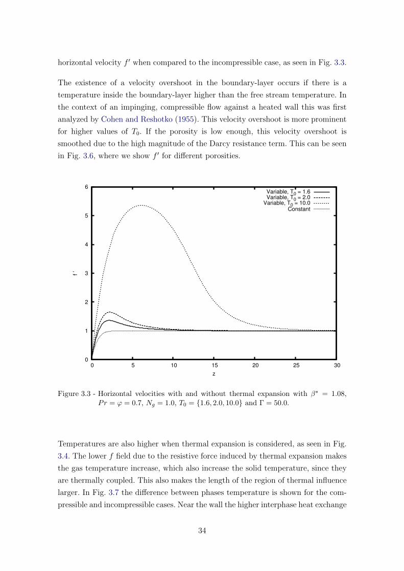
horizontal velocity f ′ when compared to the incompressible case, as seen in Fig. 3.3.
The existence of a velocity overshoot in the boundary-layer occurs if there is a
temperature inside the boundary-layer higher than the free stream temperature. In
the context of an impinging, compressible flow against a heated wall this was first
analyzed by Cohen and Reshotko (1955). This velocity overshoot is more prominent
for higher values of T0. If the porosity is low enough, this velocity overshoot is
smoothed due to the high magnitude of the Darcy resistance term. This can be seen
in Fig. 3.6, where we show f ′ for different porosities.
0
1
2
3
4
5
6
0 5 10 15 20 25 30
f ’
z
Variable, T0 = 1.6Variable, T0 = 2.0
Variable, T0 = 10.0Constant
Figure 3.3 - Horizontal velocities with and without thermal expansion with β∗ = 1.08,Pr = ϕ = 0.7, Ng = 1.0, T0 = {1.6, 2.0, 10.0} and Γ = 50.0.
Temperatures are also higher when thermal expansion is considered, as seen in Fig.
3.4. The lower f field due to the resistive force induced by thermal expansion makes
the gas temperature increase, which also increase the solid temperature, since they
are thermally coupled. This also makes the length of the region of thermal influence
larger. In Fig. 3.7 the difference between phases temperature is shown for the com-
pressible and incompressible cases. Near the wall the higher interphase heat exchange
34
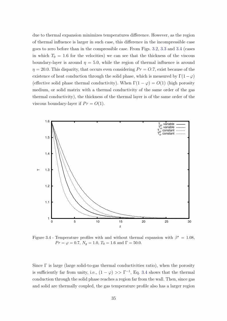
due to thermal expansion minimizes temperatures difference. However, as the region
of thermal influence is larger in such case, this difference in the incompressible case
goes to zero before than in the compressible case. From Figs. 3.2, 3.3 and 3.4 (cases
in which T0 = 1.6 for the velocities) we can see that the thickness of the viscous
boundary-layer is around η = 5.0, while the region of thermal influence is around
η = 20.0. This disparity, that occurs even considering Pr = O.7, exist because of the
existence of heat conduction through the solid phase, which is measured by Γ(1−ϕ)
(effective solid phase thermal conductivity). When Γ(1 − ϕ) = O(1) (high porosity
medium, or solid matrix with a thermal conductivity of the same order of the gas
thermal conductivity), the thickness of the thermal layer is of the same order of the
viscous boundary-layer if Pr = O(1).
1
1.1
1.2
1.3
1.4
1.5
1.6
0 5 10 15 20 25 30
T
z
Tg, variableTs, variable
Tg, constantTs, constant
Figure 3.4 - Temperature profiles with and without thermal expansion with β∗ = 1.08,Pr = ϕ = 0.7, Ng = 1.0, T0 = 1.6 and Γ = 50.0.
Since Γ is large (large solid-to-gas thermal conductivities ratio), when the porosity
is sufficiently far from unity, i.e., (1 − ϕ) >> Γ−1, Eq. 3.4 shows that the thermal
conduction through the solid phase reaches a region far from the wall. Then, since gas
and solid are thermally coupled, the gas temperature profile also has a larger region
35
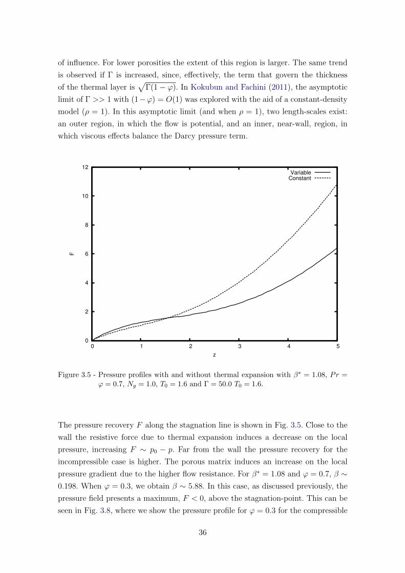
of influence. For lower porosities the extent of this region is larger. The same trend
is observed if Γ is increased, since, effectively, the term that govern the thickness
of the thermal layer is√
Γ(1− ϕ). In Kokubun and Fachini (2011), the asymptotic
limit of Γ >> 1 with (1−ϕ) = O(1) was explored with the aid of a constant-density
model (ρ = 1). In this asymptotic limit (and when ρ = 1), two length-scales exist:
an outer region, in which the flow is potential, and an inner, near-wall, region, in
which viscous effects balance the Darcy pressure term.
0
2
4
6
8
10
12
0 1 2 3 4 5
F
z
VariableConstant
Figure 3.5 - Pressure profiles with and without thermal expansion with β∗ = 1.08, Pr =ϕ = 0.7, Ng = 1.0, T0 = 1.6 and Γ = 50.0 T0 = 1.6.
The pressure recovery F along the stagnation line is shown in Fig. 3.5. Close to the
wall the resistive force due to thermal expansion induces a decrease on the local
pressure, increasing F ∼ p0 − p. Far from the wall the pressure recovery for the
incompressible case is higher. The porous matrix induces an increase on the local
pressure gradient due to the higher flow resistance. For β∗ = 1.08 and ϕ = 0.7, β ∼0.198. When ϕ = 0.3, we obtain β ∼ 5.88. In this case, as discussed previously, the
pressure field presents a maximum, F < 0, above the stagnation-point. This can be
seen in Fig. 3.8, where we show the pressure profile for ϕ = 0.3 for the compressible
36
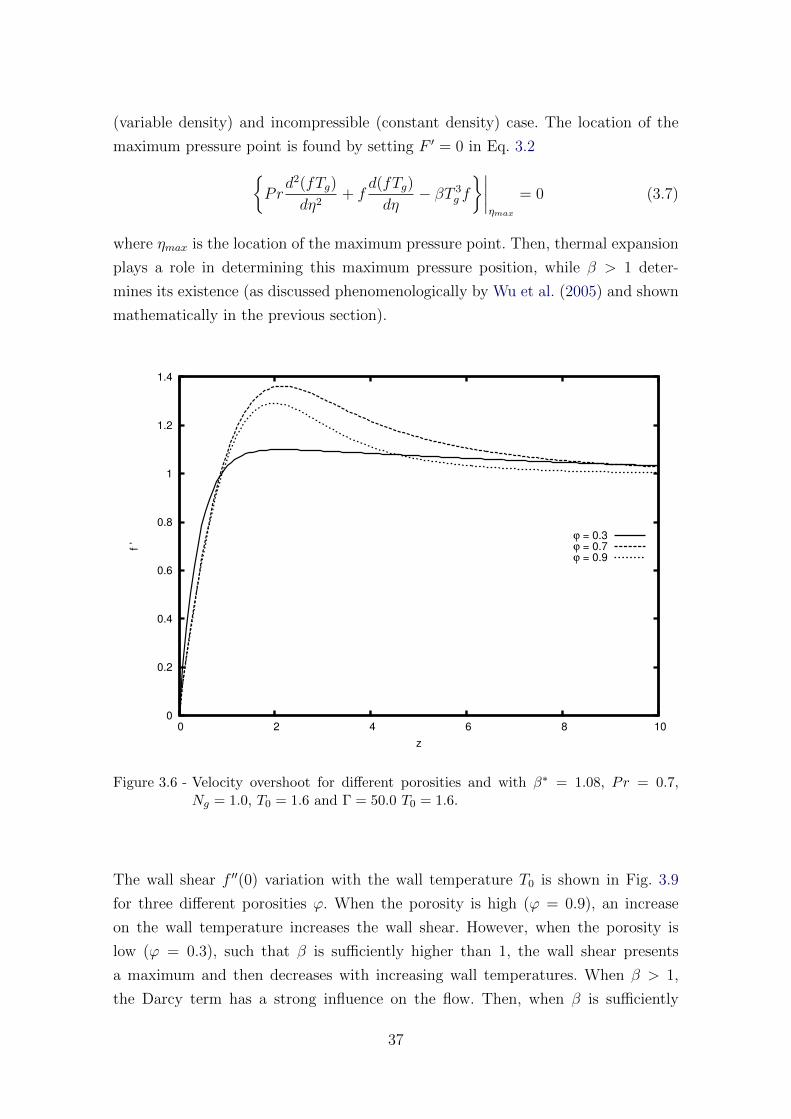
(variable density) and incompressible (constant density) case. The location of the
maximum pressure point is found by setting F ′ = 0 in Eq. 3.2{Pr
d2(fTg)
dη2+ f
d(fTg)
dη− βT 3
g f
}∣∣∣∣ηmax
= 0 (3.7)
where ηmax is the location of the maximum pressure point. Then, thermal expansion
plays a role in determining this maximum pressure position, while β > 1 deter-
mines its existence (as discussed phenomenologically by Wu et al. (2005) and shown
mathematically in the previous section).
0
0.2
0.4
0.6
0.8
1
1.2
1.4
0 2 4 6 8 10
f ’
z
ϕ = 0.3ϕ = 0.7ϕ = 0.9
Figure 3.6 - Velocity overshoot for different porosities and with β∗ = 1.08, Pr = 0.7,Ng = 1.0, T0 = 1.6 and Γ = 50.0 T0 = 1.6.
The wall shear f ′′(0) variation with the wall temperature T0 is shown in Fig. 3.9
for three different porosities ϕ. When the porosity is high (ϕ = 0.9), an increase
on the wall temperature increases the wall shear. However, when the porosity is
low (ϕ = 0.3), such that β is sufficiently higher than 1, the wall shear presents
a maximum and then decreases with increasing wall temperatures. When β > 1,
the Darcy term has a strong influence on the flow. Then, when β is sufficiently
37
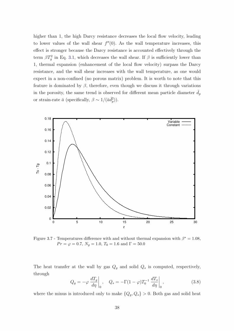
higher than 1, the high Darcy resistance decreases the local flow velocity, leading
to lower values of the wall shear f ′′(0). As the wall temperature increases, this
effect is stronger because the Darcy resistance is accounted effectively through the
term βT 2g in Eq. 3.1, which decreases the wall shear. If β is sufficiently lower than
1, thermal expansion (enhancement of the local flow velocity) surpass the Darcy
resistance, and the wall shear increases with the wall temperature, as one would
expect in a non-confined (no porous matrix) problem. It is worth to note that this
feature is dominated by β, therefore, even though we discuss it through variations
in the porosity, the same trend is observed for different mean particle diameter dp
or strain-rate a (specifically, β ∼ 1/(ad2p)).
0
0.02
0.04
0.06
0.08
0.1
0.12
0.14
0.16
0.18
0 5 10 15 20 25 30
Ts -
Tg
z
VariableConstant
Figure 3.7 - Temperatures difference with and without thermal expansion with β∗ = 1.08,Pr = ϕ = 0.7, Ng = 1.0, T0 = 1.6 and Γ = 50.0
The heat transfer at the wall by gas Qg and solid Qs is computed, respectively,
through
Qg = −ϕ dTgdη
∣∣∣∣0
, Qs = −Γ(1− ϕ)T−10
dTsdη
∣∣∣∣0
, (3.8)
where the minus is introduced only to make {Qg, Qs} > 0. Both gas and solid heat
38
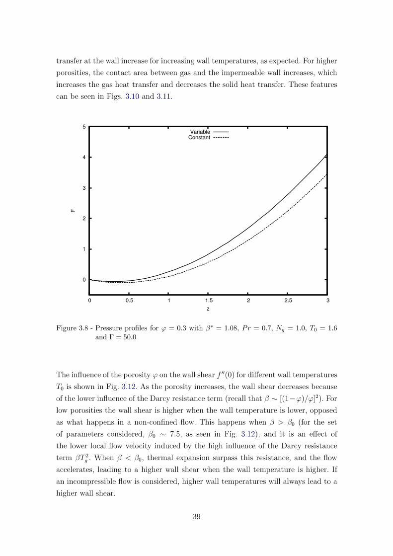
transfer at the wall increase for increasing wall temperatures, as expected. For higher
porosities, the contact area between gas and the impermeable wall increases, which
increases the gas heat transfer and decreases the solid heat transfer. These features
can be seen in Figs. 3.10 and 3.11.
0
1
2
3
4
5
0 0.5 1 1.5 2 2.5 3
F
z
VariableConstant
Figure 3.8 - Pressure profiles for ϕ = 0.3 with β∗ = 1.08, Pr = 0.7, Ng = 1.0, T0 = 1.6and Γ = 50.0
The influence of the porosity ϕ on the wall shear f ′′(0) for different wall temperatures
T0 is shown in Fig. 3.12. As the porosity increases, the wall shear decreases because
of the lower influence of the Darcy resistance term (recall that β ∼ [(1−ϕ)/ϕ]2). For
low porosities the wall shear is higher when the wall temperature is lower, opposed
as what happens in a non-confined flow. This happens when β > β0 (for the set
of parameters considered, β0 ∼ 7.5, as seen in Fig. 3.12), and it is an effect of
the lower local flow velocity induced by the high influence of the Darcy resistance
term βT 2g . When β < β0, thermal expansion surpass this resistance, and the flow
accelerates, leading to a higher wall shear when the wall temperature is higher. If
an incompressible flow is considered, higher wall temperatures will always lead to a
higher wall shear.
39
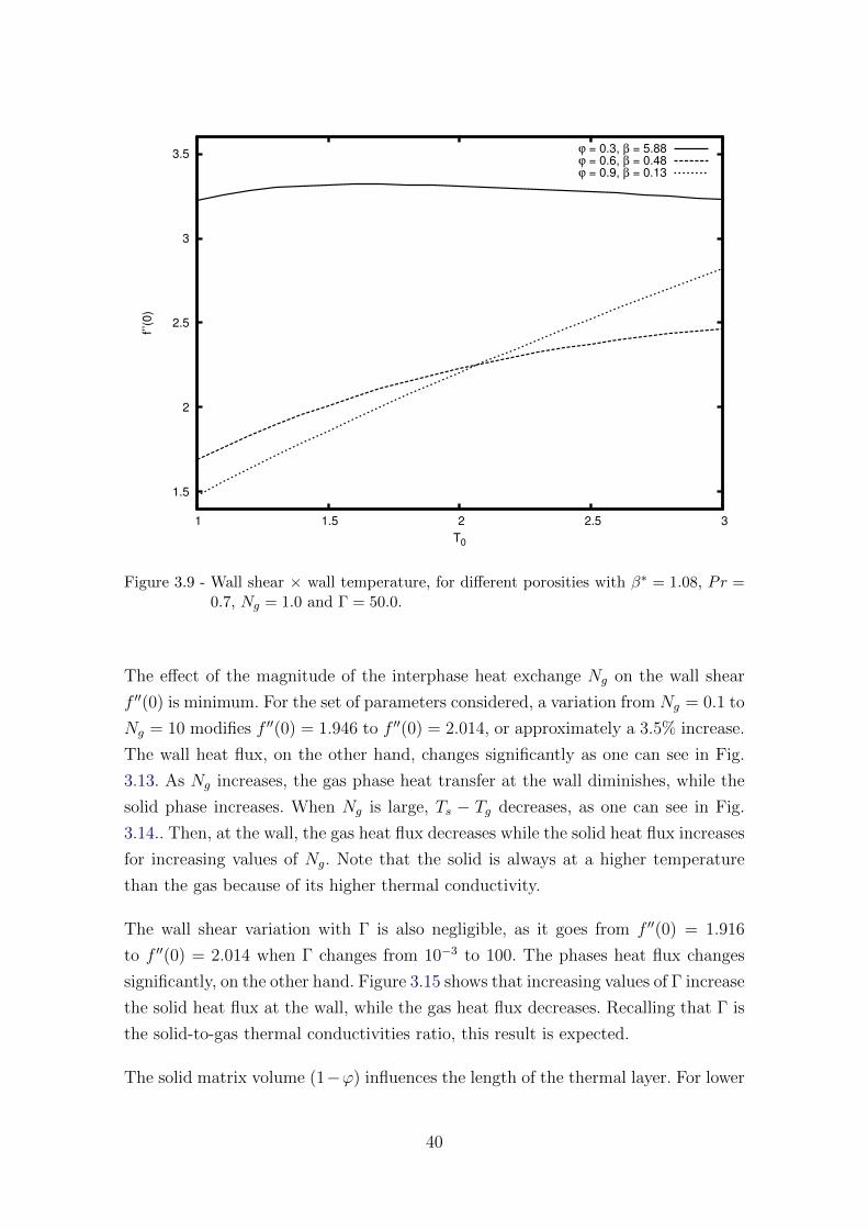
1.5
2
2.5
3
3.5
1 1.5 2 2.5 3
f’’(0)
T0
ϕ = 0.3, β = 5.88ϕ = 0.6, β = 0.48ϕ = 0.9, β = 0.13
Figure 3.9 - Wall shear × wall temperature, for different porosities with β∗ = 1.08, Pr =0.7, Ng = 1.0 and Γ = 50.0.
The effect of the magnitude of the interphase heat exchange Ng on the wall shear
f ′′(0) is minimum. For the set of parameters considered, a variation from Ng = 0.1 to
Ng = 10 modifies f ′′(0) = 1.946 to f ′′(0) = 2.014, or approximately a 3.5% increase.
The wall heat flux, on the other hand, changes significantly as one can see in Fig.
3.13. As Ng increases, the gas phase heat transfer at the wall diminishes, while the
solid phase increases. When Ng is large, Ts − Tg decreases, as one can see in Fig.
3.14.. Then, at the wall, the gas heat flux decreases while the solid heat flux increases
for increasing values of Ng. Note that the solid is always at a higher temperature
than the gas because of its higher thermal conductivity.
The wall shear variation with Γ is also negligible, as it goes from f ′′(0) = 1.916
to f ′′(0) = 2.014 when Γ changes from 10−3 to 100. The phases heat flux changes
significantly, on the other hand. Figure 3.15 shows that increasing values of Γ increase
the solid heat flux at the wall, while the gas heat flux decreases. Recalling that Γ is
the solid-to-gas thermal conductivities ratio, this result is expected.
The solid matrix volume (1−ϕ) influences the length of the thermal layer. For lower
40
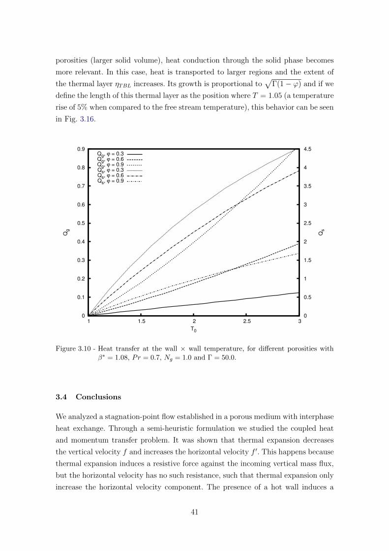
porosities (larger solid volume), heat conduction through the solid phase becomes
more relevant. In this case, heat is transported to larger regions and the extent of
the thermal layer ηTBL increases. Its growth is proportional to√
Γ(1− ϕ) and if we
define the length of this thermal layer as the position where T = 1.05 (a temperature
rise of 5% when compared to the free stream temperature), this behavior can be seen
in Fig. 3.16.
0
0.1
0.2
0.3
0.4
0.5
0.6
0.7
0.8
0.9
1 1.5 2 2.5 3 0
0.5
1
1.5
2
2.5
3
3.5
4
4.5
Qg
Qs
T0
Qg, ϕ = 0.3Qg, ϕ = 0.6Qg, ϕ = 0.9Qs, ϕ = 0.3Qs, ϕ = 0.6Qs, ϕ = 0.9
Figure 3.10 - Heat transfer at the wall × wall temperature, for different porosities withβ∗ = 1.08, Pr = 0.7, Ng = 1.0 and Γ = 50.0.
3.4 Conclusions
We analyzed a stagnation-point flow established in a porous medium with interphase
heat exchange. Through a semi-heuristic formulation we studied the coupled heat
and momentum transfer problem. It was shown that thermal expansion decreases
the vertical velocity f and increases the horizontal velocity f ′. This happens because
thermal expansion induces a resistive force against the incoming vertical mass flux,
but the horizontal velocity has no such resistance, such that thermal expansion only
increase the horizontal velocity component. The presence of a hot wall induces a
41
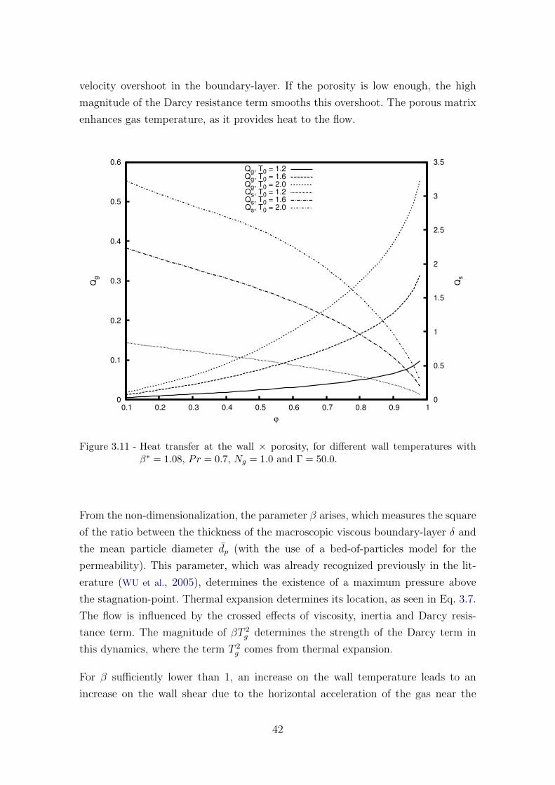
velocity overshoot in the boundary-layer. If the porosity is low enough, the high
magnitude of the Darcy resistance term smooths this overshoot. The porous matrix
enhances gas temperature, as it provides heat to the flow.
0
0.1
0.2
0.3
0.4
0.5
0.6
0.1 0.2 0.3 0.4 0.5 0.6 0.7 0.8 0.9 1 0
0.5
1
1.5
2
2.5
3
3.5
Qg
Qs
ϕ
Qg, T0 = 1.2Qg, T0 = 1.6Qg, T0 = 2.0Qs, T0 = 1.2Qs, T0 = 1.6Qs, T0 = 2.0
Figure 3.11 - Heat transfer at the wall × porosity, for different wall temperatures withβ∗ = 1.08, Pr = 0.7, Ng = 1.0 and Γ = 50.0.
From the non-dimensionalization, the parameter β arises, which measures the square
of the ratio between the thickness of the macroscopic viscous boundary-layer δ and
the mean particle diameter dp (with the use of a bed-of-particles model for the
permeability). This parameter, which was already recognized previously in the lit-
erature (WU et al., 2005), determines the existence of a maximum pressure above
the stagnation-point. Thermal expansion determines its location, as seen in Eq. 3.7.
The flow is influenced by the crossed effects of viscosity, inertia and Darcy resis-
tance term. The magnitude of βT 2g determines the strength of the Darcy term in
this dynamics, where the term T 2g comes from thermal expansion.
For β sufficiently lower than 1, an increase on the wall temperature leads to an
increase on the wall shear due to the horizontal acceleration of the gas near the
42
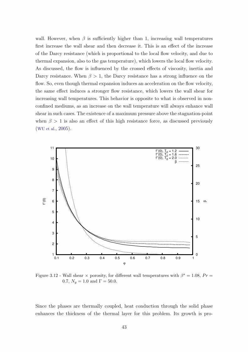
wall. However, when β is sufficiently higher than 1, increasing wall temperatures
first increase the wall shear and then decrease it. This is an effect of the increase
of the Darcy resistance (which is proportional to the local flow velocity, and due to
thermal expansion, also to the gas temperature), which lowers the local flow velocity.
As discussed, the flow is influenced by the crossed effects of viscosity, inertia and
Darcy resistance. When β > 1, the Darcy resistance has a strong influence on the
flow. So, even though thermal expansion induces an acceleration on the flow velocity,
the same effect induces a stronger flow resistance, which lowers the wall shear for
increasing wall temperatures. This behavior is opposite to what is observed in non-
confined mediums, as an increase on the wall temperature will always enhance wall
shear in such cases. The existence of a maximum pressure above the stagnation-point
when β > 1 is also an effect of this high resistance force, as discussed previously
(WU et al., 2005).
1
2
3
4
5
6
7
8
9
10
11
0.1 0.2 0.3 0.4 0.5 0.6 0.7 0.8 0.9 1 0
5
10
15
20
25
30
f’’(0)
β
ϕ
f’’(0), T0 = 1.2f’’(0), T0 = 1.6f’’(0), T0 = 2.0
β
Figure 3.12 - Wall shear × porosity, for different wall temperatures with β∗ = 1.08, Pr =0.7, Ng = 1.0 and Γ = 50.0.
Since the phases are thermally coupled, heat conduction through the solid phase
enhances the thickness of the thermal layer for this problem. Its growth is pro-
43
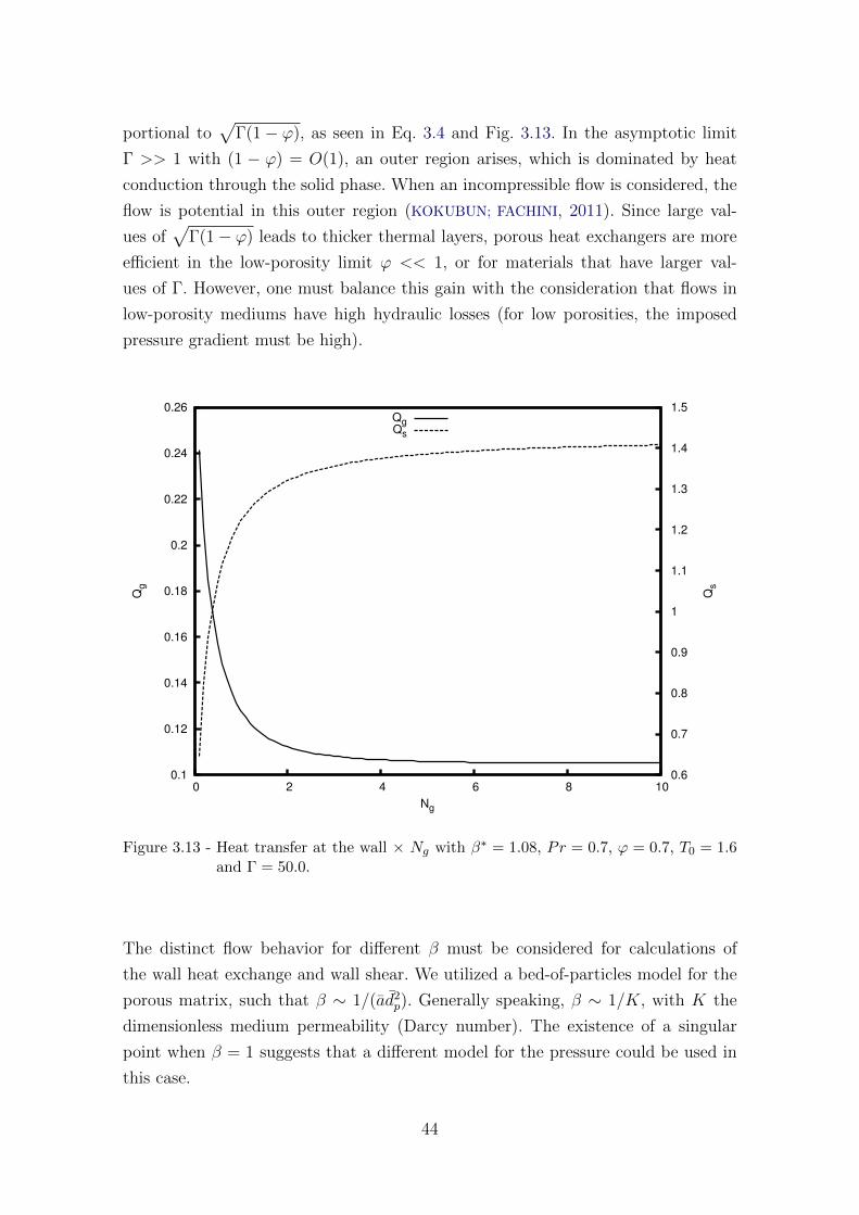
portional to√
Γ(1− ϕ), as seen in Eq. 3.4 and Fig. 3.13. In the asymptotic limit
Γ >> 1 with (1 − ϕ) = O(1), an outer region arises, which is dominated by heat
conduction through the solid phase. When an incompressible flow is considered, the
flow is potential in this outer region (KOKUBUN; FACHINI, 2011). Since large val-
ues of√
Γ(1− ϕ) leads to thicker thermal layers, porous heat exchangers are more
efficient in the low-porosity limit ϕ << 1, or for materials that have larger val-
ues of Γ. However, one must balance this gain with the consideration that flows in
low-porosity mediums have high hydraulic losses (for low porosities, the imposed
pressure gradient must be high).
0.1
0.12
0.14
0.16
0.18
0.2
0.22
0.24
0.26
0 2 4 6 8 10 0.6
0.7
0.8
0.9
1
1.1
1.2
1.3
1.4
1.5
Qg
Qs
Ng
QgQs
Figure 3.13 - Heat transfer at the wall × Ng with β∗ = 1.08, Pr = 0.7, ϕ = 0.7, T0 = 1.6and Γ = 50.0.
The distinct flow behavior for different β must be considered for calculations of
the wall heat exchange and wall shear. We utilized a bed-of-particles model for the
porous matrix, such that β ∼ 1/(ad2p). Generally speaking, β ∼ 1/K, with K the
dimensionless medium permeability (Darcy number). The existence of a singular
point when β = 1 suggests that a different model for the pressure could be used in
this case.
44
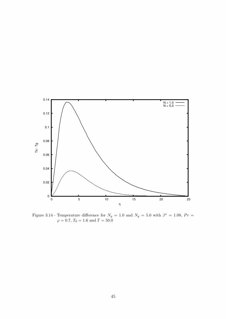
0
0.02
0.04
0.06
0.08
0.1
0.12
0.14
0 5 10 15 20 25
Ts -
Tg
η
N = 1.0N = 5.0
Figure 3.14 - Temperature difference for Ng = 1.0 and Ng = 5.0 with β∗ = 1.08, Pr =ϕ = 0.7, T0 = 1.6 and Γ = 50.0
45
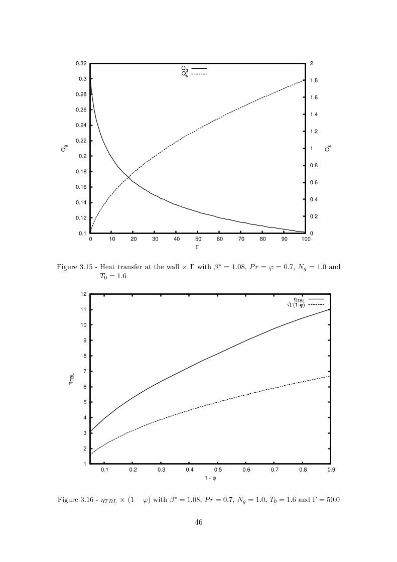
0.1
0.12
0.14
0.16
0.18
0.2
0.22
0.24
0.26
0.28
0.3
0.32
0 10 20 30 40 50 60 70 80 90 100 0
0.2
0.4
0.6
0.8
1
1.2
1.4
1.6
1.8
2Q
g
Qs
Γ
QgQs
Figure 3.15 - Heat transfer at the wall × Γ with β∗ = 1.08, Pr = ϕ = 0.7, Ng = 1.0 andT0 = 1.6
1
2
3
4
5
6
7
8
9
10
11
12
0.1 0.2 0.3 0.4 0.5 0.6 0.7 0.8 0.9
ηT
BL
1 - ϕ
ηTBL√Γ(1-ϕ)
Figure 3.16 - ηTBL × (1− ϕ) with β∗ = 1.08, Pr = 0.7, Ng = 1.0, T0 = 1.6 and Γ = 50.0
46
4 PHASE CHANGE PROBLEM: STAGNATION-POINT FLOW
AGAINST A LIQUID POOL
In this Chapter we replace the impermeable wall by a pool of liquid. The injected
gas is at a higher temperature than the liquid, that is at its boiling temperature.
Then, a steady vaporization regime is analyzed. Since we do not consider chemical
reaction to take place, the case analyzed here may be viewed as a frozen flow limit.
Studies concerning phase change in porous media are also extensively found in the
literature due to its vast amount of possible applications (YORTSOS; STUBOS, 2001).
Drying processes (DAURELLE et al., 1998), geothermal systems (WOODS, 1999) and
nuclear safety issues are some examples of such system. The evaporation of a thin
film of liquid water within a heated porous bed subjected to a stagnation-point flow
was studied analytically (ZHAO, 1999). In that work, the coupled heat and mass
transfer problem was analyzed in the proposed geometry. Local thermal equilibrium
was considered, and the focus was on the parameters influence on the heat and mass
transfer properties. The obtained results are of significance for the design of indirect
evaporative air cooler systems.
Boiling in a saturated porous medium was analyzed by Ramesh and Torrance (1993)
by considering a heat supply from below and a cooling from above. Using numer-
ical methods, they analyzed the possible flow regimes with the consideration of a
moving liquid/two-phase interface. The authors conducted a parametric study con-
sidering the liquid-phase Rayleigh number and the non-dimensional bottom heat
flux. Their results recognized three different regimes: conduction-dominated for low
Rayleigh number, convection-dominated for intermediary Rayleigh number, and os-
cillatory convection for high Rayleigh number. In the convection-dominated regime,
as the non-dimensional bottom heat flux increases, transitions to multiple cell pat-
terns were observed. The stability of the obtained solutions to perturbations was
also conducted. The interphase heat exchange was considered fixed as a heat loss
parameter.
Effects of local thermal non-equilibrium on the infiltration of a hot fluid into a cold
porous medium was analyzed by Rees et al. (2008). In order to study this flow
configuration, the moving thermal front resultant from the thermal non-equilibrium
was analyzed. By performing a scale analysis and numerical simulations, the dif-
ferent manners in which the temperature fields evolve in time were discussed. It
was found that the thickness of the thermal front is a function of the governing
parameters (namely, the non-dimensional interphase heat transfer parameter, the
47
porosity-modified conductivity ratio and the diffusivity ratio). This has the implica-
tion that local thermal equilibrium is not equivalent to a single equation formulation
of the energy equation. Their results for a large-time analysis showed that local ther-
mal equilibrium is achieved in such limit, but in a solution different from that which
would be obtained by an one-equation modeling. It was also observed the formation
of a shock wave when the velocity of the infiltrating fluid was sufficiently large.
There is also a good amount of studies in the open literature concerning natural
evaporation, specially concerning the analysis of drying of porous media. Such prob-
lem finds applications to areas such as wood, paper, and the textile industry. Il´ichev
et al. (2008) studied the gravitational instability of the salinity profile during the
evaporation of saline groundwater. The stability analysis concluded that the most
significant effect controlling the stability is the permeability of the soil. The effects
of the different characteristic length scales in the problem of evaporative drying of
a porous medium was analyzed by Lehmann et al. (2008). By comparing the roles
of gravity, capillarity and viscous dissipation forces, they deduced the characteristic
length for the maximum hydraulically connected film region between the drying front
and the surface. The characteristic lengths depend on the size range between the
smallest and largest pores within the film region. For media with large pores sizes,
the characteristic length is dominated by gravity and capillarity, and the viscous dis-
sipation is negligible. For media with small pores sizes (fine-textured) it was shown
that viscous dissipation may limit the maximum hydraulically connected distance
between the drying front and the evaporating surface. The authors also conducted
experiments with two types of sand in order to determine the characteristic lengths
and the extent of the film region.
The situation when heat is supplied to the condensed phase by a hot impinging gas
arise, for instance, in the steam injection process of thermal oil recovery (NARAYAN;
WALSH, 1988; JABBOUR et al., 1996). When a well contains heavy oil, its recovery may
be achieved by means of heat addition in the reservoir, increasing its temperature
and lowering the oil viscosity and hence increasing its mobility. The initial (injection)
temperature of the steam must be high.
Heavy-oils have low volatility, such that the enhancement of the vaporization rate
caused by heat transport through the solid phase is the main responsible for its
phase change. In the context of a constant-density model and in the limit Γ >>
1 (asymptotically large solid-to-gas thermal conductivities ratio), a liquid of l =
O(Γ) >> 1 (very low volatility) was considered previously (KOKUBUN; FACHINI,
48
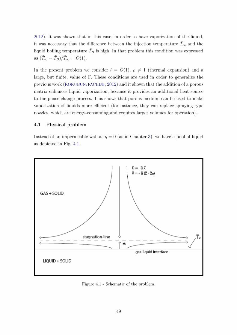
2012). It was shown that in this case, in order to have vaporization of the liquid,
it was necessary that the difference between the injection temperature T∞ and the
liquid boiling temperature TB is high. In that problem this condition was expressed
as (T∞ − TB)/T∞ = O(1).
In the present problem we consider l = O(1), ρ 6= 1 (thermal expansion) and a
large, but finite, value of Γ. These conditions are used in order to generalize the
previous work (KOKUBUN; FACHINI, 2012) and it shown that the addition of a porous
matrix enhances liquid vaporization, because it provides an additional heat source
to the phase change process. This shows that porous-medium can be used to make
vaporization of liquids more efficient (for instance, they can replace spraying-type
nozzles, which are energy-consuming and requires larger volumes for operation).
4.1 Physical problem
Instead of an impermeable wall at η = 0 (as in Chapter 3), we have a pool of liquid
as depicted in Fig. 4.1.
Figure 4.1 - Schematic of the problem.
49
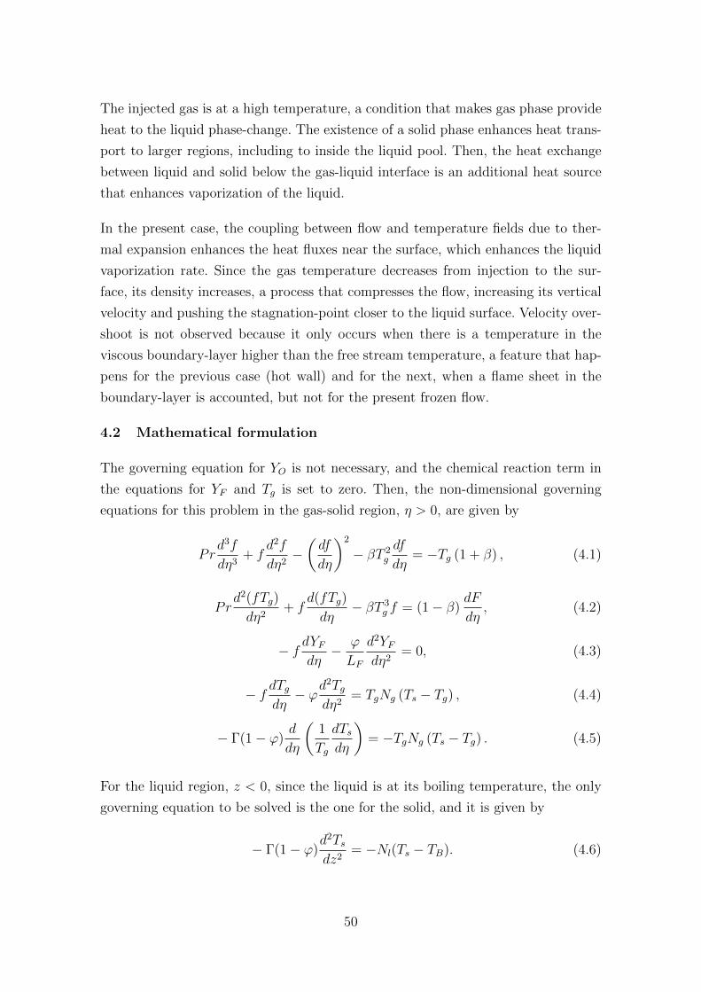
The injected gas is at a high temperature, a condition that makes gas phase provide
heat to the liquid phase-change. The existence of a solid phase enhances heat trans-
port to larger regions, including to inside the liquid pool. Then, the heat exchange
between liquid and solid below the gas-liquid interface is an additional heat source
that enhances vaporization of the liquid.
In the present case, the coupling between flow and temperature fields due to ther-
mal expansion enhances the heat fluxes near the surface, which enhances the liquid
vaporization rate. Since the gas temperature decreases from injection to the sur-
face, its density increases, a process that compresses the flow, increasing its vertical
velocity and pushing the stagnation-point closer to the liquid surface. Velocity over-
shoot is not observed because it only occurs when there is a temperature in the
viscous boundary-layer higher than the free stream temperature, a feature that hap-
pens for the previous case (hot wall) and for the next, when a flame sheet in the
boundary-layer is accounted, but not for the present frozen flow.
4.2 Mathematical formulation
The governing equation for YO is not necessary, and the chemical reaction term in
the equations for YF and Tg is set to zero. Then, the non-dimensional governing
equations for this problem in the gas-solid region, η > 0, are given by
Prd3f
dη3+ f
d2f
dη2−(df
dη
)2
− βT 2g
df
dη= −Tg (1 + β) , (4.1)
Prd2(fTg)
dη2+ f
d(fTg)
dη− βT 3
g f = (1− β)dF
dη, (4.2)
− f dYFdη− ϕ
LF
d2YFdη2
= 0, (4.3)
− f dTgdη− ϕd
2Tgdη2
= TgNg (Ts − Tg) , (4.4)
− Γ(1− ϕ)d
dη
(1
Tg
dTsdη
)= −TgNg (Ts − Tg) . (4.5)
For the liquid region, z < 0, since the liquid is at its boiling temperature, the only
governing equation to be solved is the one for the solid, and it is given by
− Γ(1− ϕ)d2Tsdz2
= −Nl(Ts − TB). (4.6)
50
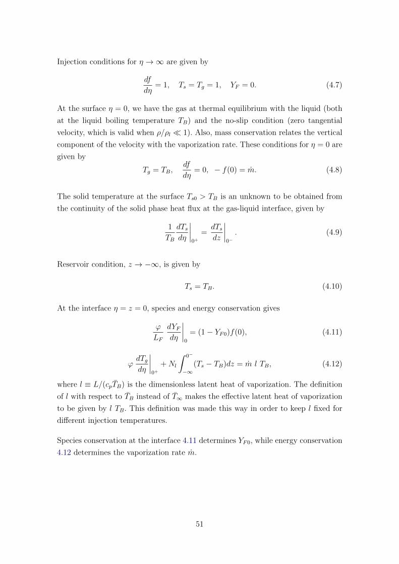
Injection conditions for η →∞ are given by
df
dη= 1, Ts = Tg = 1, YF = 0. (4.7)
At the surface η = 0, we have the gas at thermal equilibrium with the liquid (both
at the liquid boiling temperature TB) and the no-slip condition (zero tangential
velocity, which is valid when ρ/ρl � 1). Also, mass conservation relates the vertical
component of the velocity with the vaporization rate. These conditions for η = 0 are
given by
Tg = TB,df
dη= 0, − f(0) = m. (4.8)
The solid temperature at the surface Ts0 > TB is an unknown to be obtained from
the continuity of the solid phase heat flux at the gas-liquid interface, given by
1
TB
dTsdη
∣∣∣∣0+
=dTsdz
∣∣∣∣0−. (4.9)
Reservoir condition, z → −∞, is given by
Ts = TB. (4.10)
At the interface η = z = 0, species and energy conservation gives
ϕ
LF
dYFdη
∣∣∣∣0
= (1− YF0)f(0), (4.11)
ϕdTgdη
∣∣∣∣0+
+Nl
∫ 0−
−∞(Ts − TB)dz = m l TB, (4.12)
where l ≡ L/(cpTB) is the dimensionless latent heat of vaporization. The definition
of l with respect to TB instead of T∞ makes the effective latent heat of vaporization
to be given by l TB. This definition was made this way in order to keep l fixed for
different injection temperatures.
Species conservation at the interface 4.11 determines YF0, while energy conservation
4.12 determines the vaporization rate m.
51
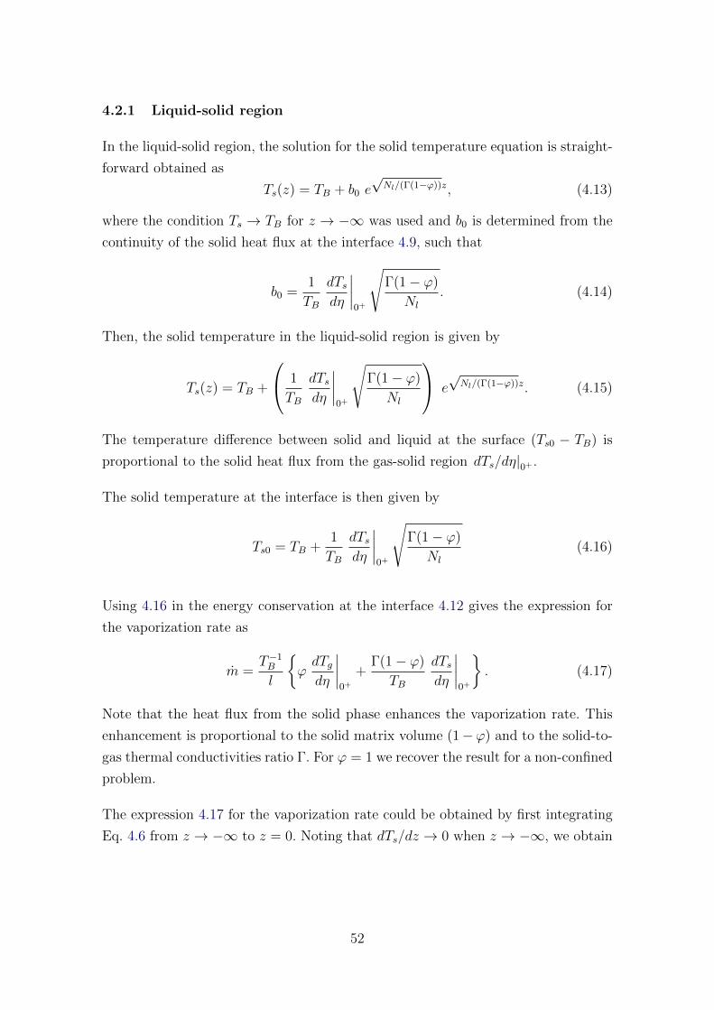
4.2.1 Liquid-solid region
In the liquid-solid region, the solution for the solid temperature equation is straight-
forward obtained as
Ts(z) = TB + b0 e√Nl/(Γ(1−ϕ))z, (4.13)
where the condition Ts → TB for z → −∞ was used and b0 is determined from the
continuity of the solid heat flux at the interface 4.9, such that
b0 =1
TB
dTsdη
∣∣∣∣0+
√Γ(1− ϕ)
Nl
. (4.14)
Then, the solid temperature in the liquid-solid region is given by
Ts(z) = TB +
1
TB
dTsdη
∣∣∣∣0+
√Γ(1− ϕ)
Nl
e√Nl/(Γ(1−ϕ))z. (4.15)
The temperature difference between solid and liquid at the surface (Ts0 − TB) is
proportional to the solid heat flux from the gas-solid region dTs/dη|0+ .
The solid temperature at the interface is then given by
Ts0 = TB +1
TB
dTsdη
∣∣∣∣0+
√Γ(1− ϕ)
Nl
(4.16)
Using 4.16 in the energy conservation at the interface 4.12 gives the expression for
the vaporization rate as
m =T−1B
l
{ϕdTgdη
∣∣∣∣0+
+Γ(1− ϕ)
TB
dTsdη
∣∣∣∣0+
}. (4.17)
Note that the heat flux from the solid phase enhances the vaporization rate. This
enhancement is proportional to the solid matrix volume (1−ϕ) and to the solid-to-
gas thermal conductivities ratio Γ. For ϕ = 1 we recover the result for a non-confined
problem.
The expression 4.17 for the vaporization rate could be obtained by first integrating
Eq. 4.6 from z → −∞ to z = 0. Noting that dTs/dz → 0 when z → −∞, we obtain
52
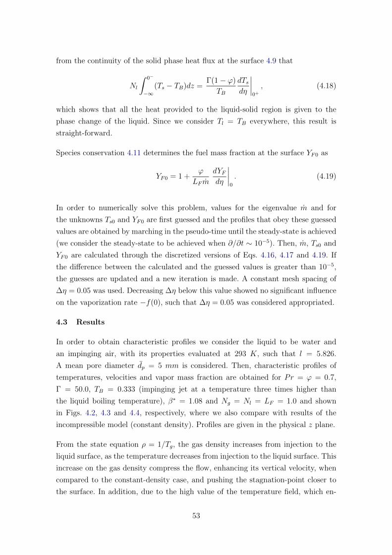
from the continuity of the solid phase heat flux at the surface 4.9 that
Nl
∫ 0−
−∞(Ts − TB)dz =
Γ(1− ϕ)
TB
dTsdη
∣∣∣∣0+, (4.18)
which shows that all the heat provided to the liquid-solid region is given to the
phase change of the liquid. Since we consider Tl = TB everywhere, this result is
straight-forward.
Species conservation 4.11 determines the fuel mass fraction at the surface YF0 as
YF0 = 1 +ϕ
LF m
dYFdη
∣∣∣∣0
. (4.19)
In order to numerically solve this problem, values for the eigenvalue m and for
the unknowns Ts0 and YF0 are first guessed and the profiles that obey these guessed
values are obtained by marching in the pseudo-time until the steady-state is achieved
(we consider the steady-state to be achieved when ∂/∂t ∼ 10−5). Then, m, Ts0 and
YF0 are calculated through the discretized versions of Eqs. 4.16, 4.17 and 4.19. If
the difference between the calculated and the guessed values is greater than 10−5,
the guesses are updated and a new iteration is made. A constant mesh spacing of
∆η = 0.05 was used. Decreasing ∆η below this value showed no significant influence
on the vaporization rate −f(0), such that ∆η = 0.05 was considered appropriated.
4.3 Results
In order to obtain characteristic profiles we consider the liquid to be water and
an impinging air, with its properties evaluated at 293 K, such that l = 5.826.
A mean pore diameter dp = 5 mm is considered. Then, characteristic profiles of
temperatures, velocities and vapor mass fraction are obtained for Pr = ϕ = 0.7,
Γ = 50.0, TB = 0.333 (impinging jet at a temperature three times higher than
the liquid boiling temperature), β∗ = 1.08 and Ng = Nl = LF = 1.0 and shown
in Figs. 4.2, 4.3 and 4.4, respectively, where we also compare with results of the
incompressible model (constant density). Profiles are given in the physical z plane.
From the state equation ρ = 1/Tg, the gas density increases from injection to the
liquid surface, as the temperature decreases from injection to the liquid surface. This
increase on the gas density compress the flow, enhancing its vertical velocity, when
compared to the constant-density case, and pushing the stagnation-point closer to
the surface. In addition, due to the high value of the temperature field, which en-
53
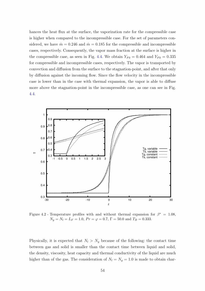
hances the heat flux at the surface, the vaporization rate for the compressible case
is higher when compared to the incompressible case. For the set of parameters con-
sidered, we have m = 0.246 and m = 0.185 for the compressible and incompressible
cases, respectively. Consequently, the vapor mass fraction at the surface is higher in
the compressible case, as seen in Fig. 4.4. We obtain YF0 = 0.464 and YF0 = 0.335
for compressible and incompressible cases, respectively. The vapor is transported by
convection and diffusion from the surface to the stagnation-point, and after that only
by diffusion against the incoming flow. Since the flow velocity in the incompressible
case is lower than in the case with thermal expansion, the vapor is able to diffuse
more above the stagnation-point in the incompressible case, as one can see in Fig.
4.4.
0.3
0.4
0.5
0.6
0.7
0.8
0.9
1
-30 -20 -10 0 10 20 30
T
z
Tg, variableTs, variable
Tg, constantTs, constant
0.3
0.4
0.5
0.6
0.7
0.8
0.9
-1 -0.5 0 0.5 1 1.5 2 2.5 3
Figure 4.2 - Temperature profiles with and without thermal expansion for β∗ = 1.08,Ng = Nl = LF = 1.0, Pr = ϕ = 0.7, Γ = 50.0 and TB = 0.333.
Physically, it is expected that Nl > Ng because of the following: the contact time
between gas and solid is smaller than the contact time between liquid and solid,
the density, viscosity, heat capacity and thermal conductivity of the liquid are much
higher than of the gas. The consideration of Nl = Ng = 1.0 is made to obtain char-
54
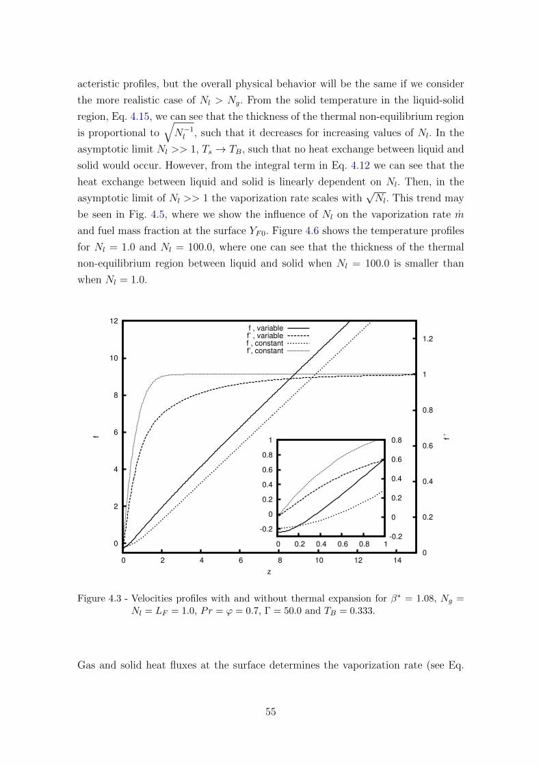
acteristic profiles, but the overall physical behavior will be the same if we consider
the more realistic case of Nl > Ng. From the solid temperature in the liquid-solid
region, Eq. 4.15, we can see that the thickness of the thermal non-equilibrium region
is proportional to√N−1l , such that it decreases for increasing values of Nl. In the
asymptotic limit Nl >> 1, Ts → TB, such that no heat exchange between liquid and
solid would occur. However, from the integral term in Eq. 4.12 we can see that the
heat exchange between liquid and solid is linearly dependent on Nl. Then, in the
asymptotic limit of Nl >> 1 the vaporization rate scales with√Nl. This trend may
be seen in Fig. 4.5, where we show the influence of Nl on the vaporization rate m
and fuel mass fraction at the surface YF0. Figure 4.6 shows the temperature profiles
for Nl = 1.0 and Nl = 100.0, where one can see that the thickness of the thermal
non-equilibrium region between liquid and solid when Nl = 100.0 is smaller than
when Nl = 1.0.
0
2
4
6
8
10
12
0 2 4 6 8 10 12 14 0
0.2
0.4
0.6
0.8
1
1.2
f
f ’
z
f , variablef’ , variablef , constantf’, constant
-0.2
0
0.2
0.4
0.6
0.8
1
0 0.2 0.4 0.6 0.8 1-0.2
0
0.2
0.4
0.6
0.8
Figure 4.3 - Velocities profiles with and without thermal expansion for β∗ = 1.08, Ng =Nl = LF = 1.0, Pr = ϕ = 0.7, Γ = 50.0 and TB = 0.333.
Gas and solid heat fluxes at the surface determines the vaporization rate (see Eq.
55
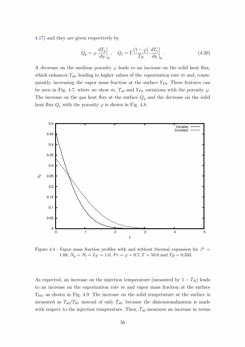
4.17) and they are given respectively by
Qg = ϕdTgdη
∣∣∣∣0
, Qs = Γ(1− ϕ)
TB
dTsdη
∣∣∣∣0
. (4.20)
A decrease on the medium porosity ϕ leads to an increase on the solid heat flux,
which enhances Ts0, leading to higher values of the vaporization rate m and, conse-
quently, increasing the vapor mass fraction at the surface YF0. These features can
be seen in Fig. 4.7, where we show m, Ts0 and YF0 variations with the porosity ϕ.
The increase on the gas heat flux at the surface Qg and the decrease on the solid
heat flux Qs with the porosity ϕ is shown in Fig. 4.8.
0
0.05
0.1
0.15
0.2
0.25
0.3
0.35
0.4
0.45
0.5
0 1 2 3 4 5
YF
z
VariableConstant
Figure 4.4 - Vapor mass fraction profiles with and without thermal expansion for β∗ =1.08, Ng = Nl = LF = 1.0, Pr = ϕ = 0.7, Γ = 50.0 and TB = 0.333.
As expected, an increase on the injection temperature (measured by 1 − TB) leads
to an increase on the vaporization rate m and vapor mass fraction at the surface
YF0, as shown in Fig. 4.9. The increase on the solid temperature at the surface is
measured as Ts0/TB, instead of only Ts0, because the dimensionalization is made
with respect to the injection temperature. Then, Ts0 measures an increase in terms
56
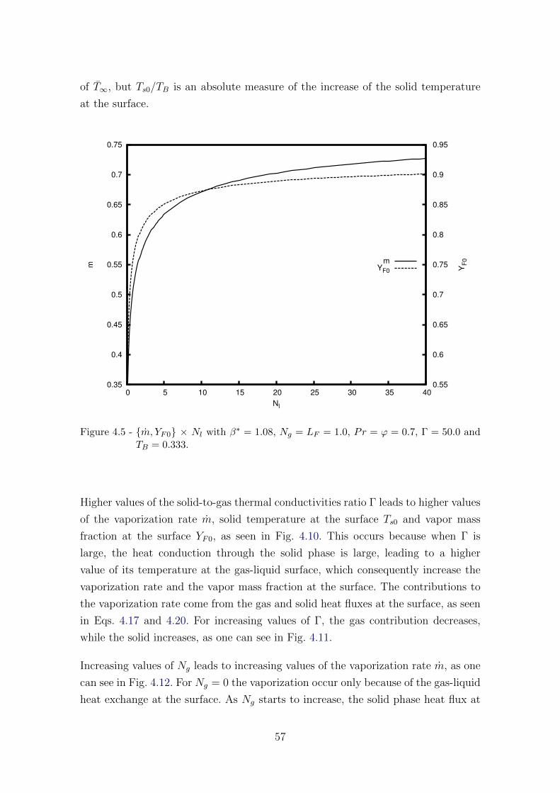
of T∞, but Ts0/TB is an absolute measure of the increase of the solid temperature
at the surface.
0.35
0.4
0.45
0.5
0.55
0.6
0.65
0.7
0.75
0 5 10 15 20 25 30 35 40 0.55
0.6
0.65
0.7
0.75
0.8
0.85
0.9
0.95
m YF
0
Nl
mYF0
Figure 4.5 - {m, YF0} × Nl with β∗ = 1.08, Ng = LF = 1.0, Pr = ϕ = 0.7, Γ = 50.0 andTB = 0.333.
Higher values of the solid-to-gas thermal conductivities ratio Γ leads to higher values
of the vaporization rate m, solid temperature at the surface Ts0 and vapor mass
fraction at the surface YF0, as seen in Fig. 4.10. This occurs because when Γ is
large, the heat conduction through the solid phase is large, leading to a higher
value of its temperature at the gas-liquid surface, which consequently increase the
vaporization rate and the vapor mass fraction at the surface. The contributions to
the vaporization rate come from the gas and solid heat fluxes at the surface, as seen
in Eqs. 4.17 and 4.20. For increasing values of Γ, the gas contribution decreases,
while the solid increases, as one can see in Fig. 4.11.
Increasing values of Ng leads to increasing values of the vaporization rate m, as one
can see in Fig. 4.12. For Ng = 0 the vaporization occur only because of the gas-liquid
heat exchange at the surface. As Ng starts to increase, the solid phase heat flux at
57
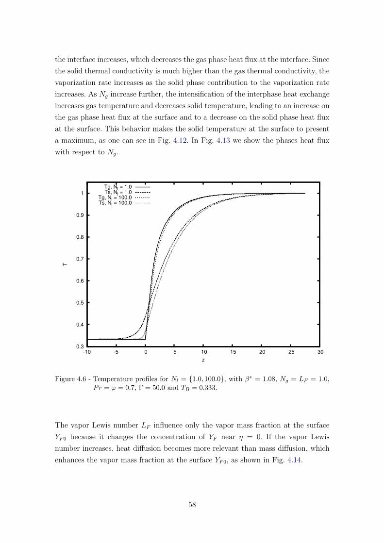
the interface increases, which decreases the gas phase heat flux at the interface. Since
the solid thermal conductivity is much higher than the gas thermal conductivity, the
vaporization rate increases as the solid phase contribution to the vaporization rate
increases. As Ng increase further, the intensification of the interphase heat exchange
increases gas temperature and decreases solid temperature, leading to an increase on
the gas phase heat flux at the surface and to a decrease on the solid phase heat flux
at the surface. This behavior makes the solid temperature at the surface to present
a maximum, as one can see in Fig. 4.12. In Fig. 4.13 we show the phases heat flux
with respect to Ng.
0.3
0.4
0.5
0.6
0.7
0.8
0.9
1
-10 -5 0 5 10 15 20 25 30
T
z
Tg, Nl = 1.0Ts, Nl = 1.0
Tg, Nl = 100.0Ts, Nl = 100.0
Figure 4.6 - Temperature profiles for Nl = {1.0, 100.0}, with β∗ = 1.08, Ng = LF = 1.0,Pr = ϕ = 0.7, Γ = 50.0 and TB = 0.333.
The vapor Lewis number LF influence only the vapor mass fraction at the surface
YF0 because it changes the concentration of YF near η = 0. If the vapor Lewis
number increases, heat diffusion becomes more relevant than mass diffusion, which
enhances the vapor mass fraction at the surface YF0, as shown in Fig. 4.14.
58
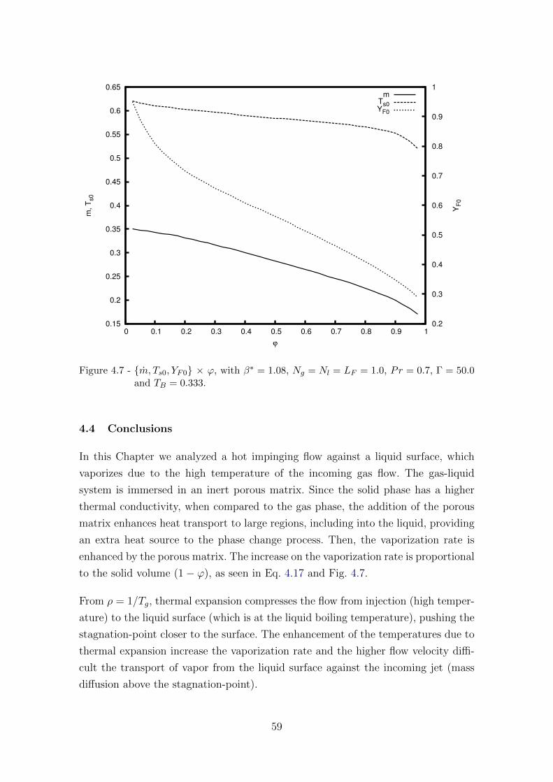
0.15
0.2
0.25
0.3
0.35
0.4
0.45
0.5
0.55
0.6
0.65
0 0.1 0.2 0.3 0.4 0.5 0.6 0.7 0.8 0.9 1 0.2
0.3
0.4
0.5
0.6
0.7
0.8
0.9
1m
, T
s0
YF
0
ϕ
mTs0YF0
Figure 4.7 - {m, Ts0, YF0} × ϕ, with β∗ = 1.08, Ng = Nl = LF = 1.0, Pr = 0.7, Γ = 50.0and TB = 0.333.
4.4 Conclusions
In this Chapter we analyzed a hot impinging flow against a liquid surface, which
vaporizes due to the high temperature of the incoming gas flow. The gas-liquid
system is immersed in an inert porous matrix. Since the solid phase has a higher
thermal conductivity, when compared to the gas phase, the addition of the porous
matrix enhances heat transport to large regions, including into the liquid, providing
an extra heat source to the phase change process. Then, the vaporization rate is
enhanced by the porous matrix. The increase on the vaporization rate is proportional
to the solid volume (1− ϕ), as seen in Eq. 4.17 and Fig. 4.7.
From ρ = 1/Tg, thermal expansion compresses the flow from injection (high temper-
ature) to the liquid surface (which is at the liquid boiling temperature), pushing the
stagnation-point closer to the surface. The enhancement of the temperatures due to
thermal expansion increase the vaporization rate and the higher flow velocity diffi-
cult the transport of vapor from the liquid surface against the incoming jet (mass
diffusion above the stagnation-point).
59
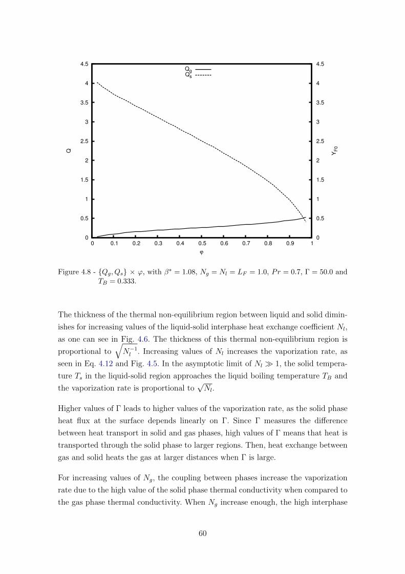
0
0.5
1
1.5
2
2.5
3
3.5
4
4.5
0 0.1 0.2 0.3 0.4 0.5 0.6 0.7 0.8 0.9 1 0
0.5
1
1.5
2
2.5
3
3.5
4
4.5Q YF
0
ϕ
QgQs
Figure 4.8 - {Qg, Qs} × ϕ, with β∗ = 1.08, Ng = Nl = LF = 1.0, Pr = 0.7, Γ = 50.0 andTB = 0.333.
The thickness of the thermal non-equilibrium region between liquid and solid dimin-
ishes for increasing values of the liquid-solid interphase heat exchange coefficient Nl,
as one can see in Fig. 4.6. The thickness of this thermal non-equilibrium region is
proportional to√N−1l . Increasing values of Nl increases the vaporization rate, as
seen in Eq. 4.12 and Fig. 4.5. In the asymptotic limit of Nl � 1, the solid tempera-
ture Ts in the liquid-solid region approaches the liquid boiling temperature TB and
the vaporization rate is proportional to√Nl.
Higher values of Γ leads to higher values of the vaporization rate, as the solid phase
heat flux at the surface depends linearly on Γ. Since Γ measures the difference
between heat transport in solid and gas phases, high values of Γ means that heat is
transported through the solid phase to larger regions. Then, heat exchange between
gas and solid heats the gas at larger distances when Γ is large.
For increasing values of Ng, the coupling between phases increase the vaporization
rate due to the high value of the solid phase thermal conductivity when compared to
the gas phase thermal conductivity. When Ng increase enough, the high interphase
60
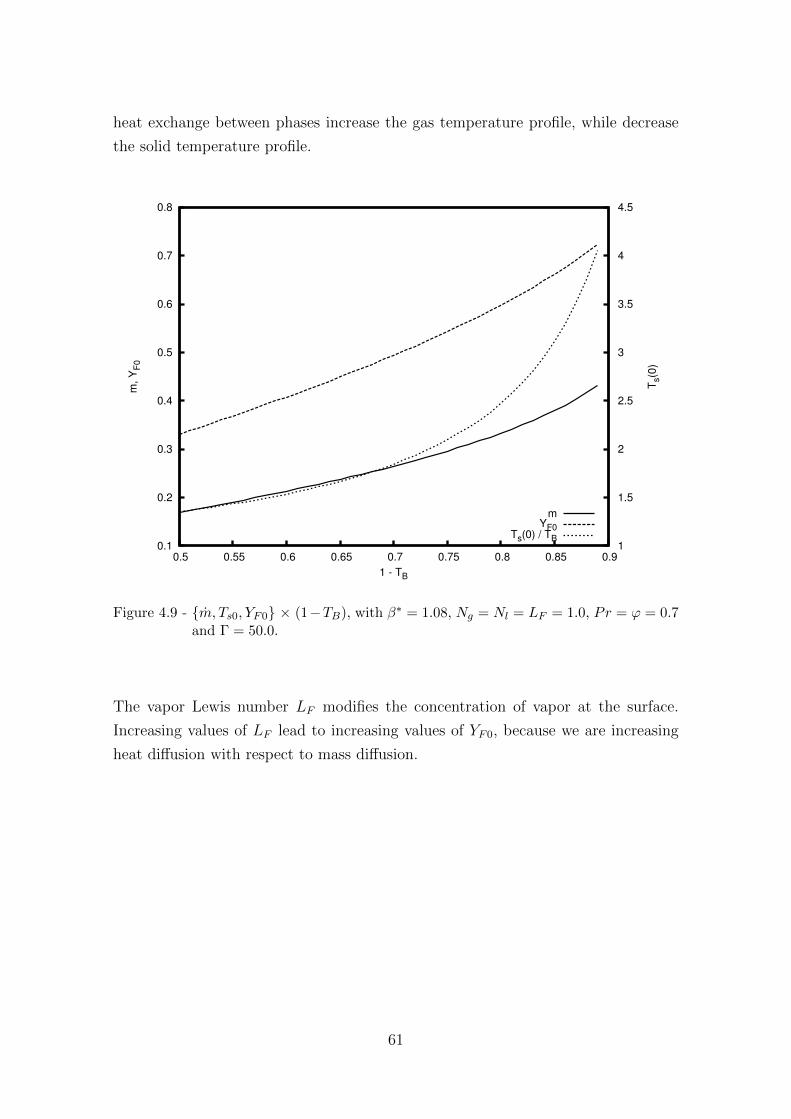
heat exchange between phases increase the gas temperature profile, while decrease
the solid temperature profile.
0.1
0.2
0.3
0.4
0.5
0.6
0.7
0.8
0.5 0.55 0.6 0.65 0.7 0.75 0.8 0.85 0.9 1
1.5
2
2.5
3
3.5
4
4.5
m, Y
F0
Ts(0
)
1 - TB
mYF0
Ts(0) / TB
Figure 4.9 - {m, Ts0, YF0} × (1−TB), with β∗ = 1.08, Ng = Nl = LF = 1.0, Pr = ϕ = 0.7and Γ = 50.0.
The vapor Lewis number LF modifies the concentration of vapor at the surface.
Increasing values of LF lead to increasing values of YF0, because we are increasing
heat diffusion with respect to mass diffusion.
61
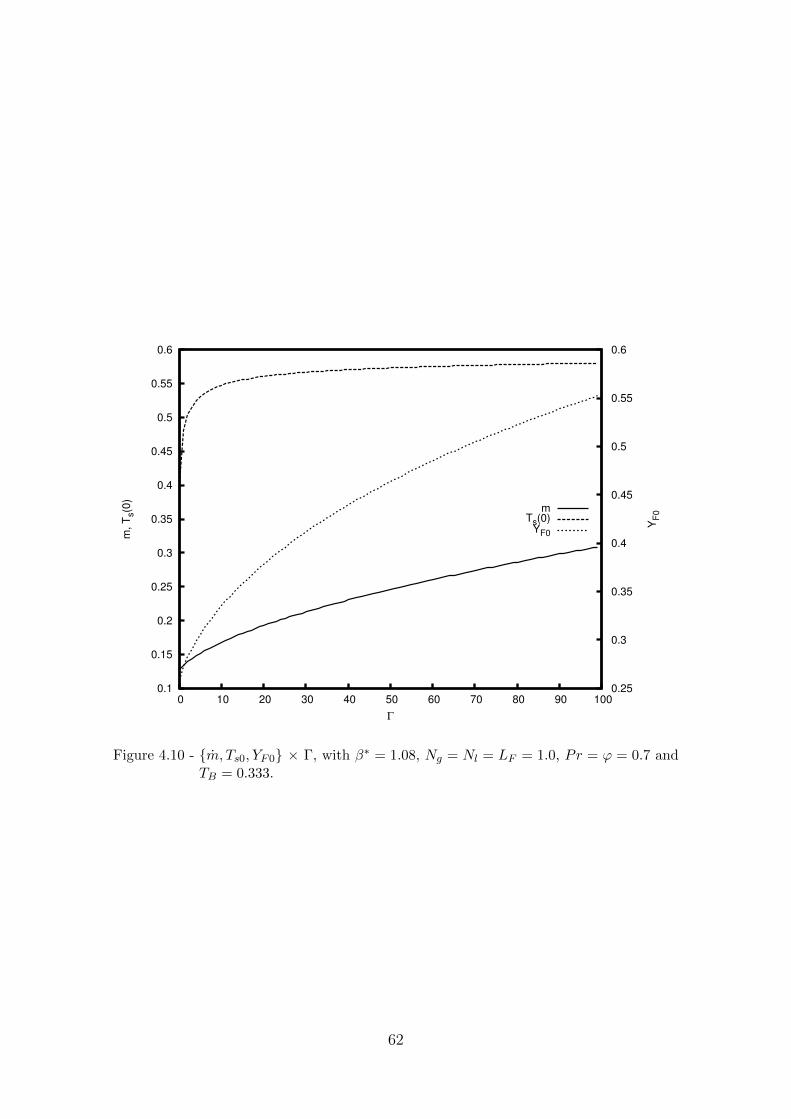
0.1
0.15
0.2
0.25
0.3
0.35
0.4
0.45
0.5
0.55
0.6
0 10 20 30 40 50 60 70 80 90 100 0.25
0.3
0.35
0.4
0.45
0.5
0.55
0.6
m, T
s(0
)
YF
0
Γ
mTs(0)
YF0
Figure 4.10 - {m, Ts0, YF0} × Γ, with β∗ = 1.08, Ng = Nl = LF = 1.0, Pr = ϕ = 0.7 andTB = 0.333.
62
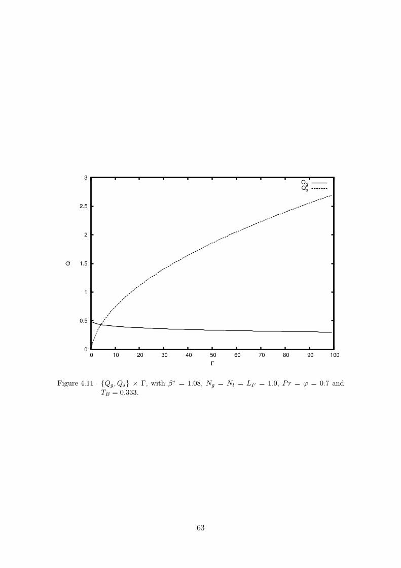
0
0.5
1
1.5
2
2.5
3
0 10 20 30 40 50 60 70 80 90 100
Q
Γ
QgQs
Figure 4.11 - {Qg, Qs} × Γ, with β∗ = 1.08, Ng = Nl = LF = 1.0, Pr = ϕ = 0.7 andTB = 0.333.
63
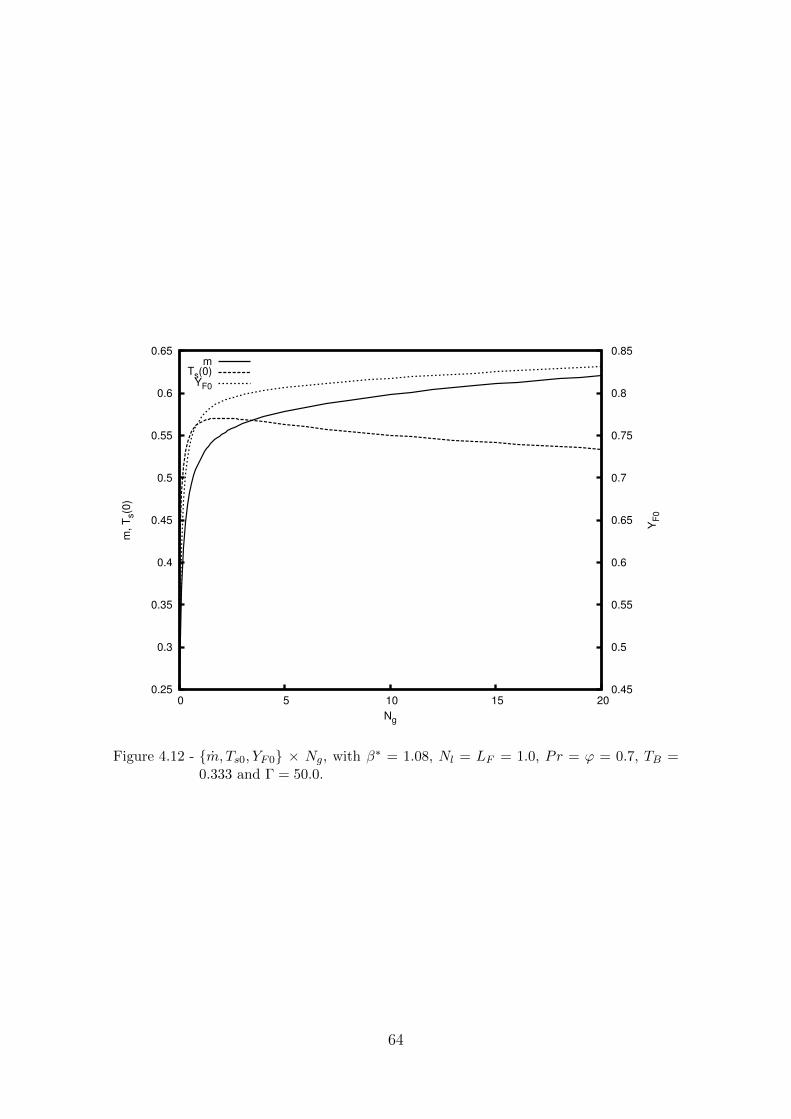
0.25
0.3
0.35
0.4
0.45
0.5
0.55
0.6
0.65
0 5 10 15 20 0.45
0.5
0.55
0.6
0.65
0.7
0.75
0.8
0.85
m, T
s(0
)
YF
0
Ng
mTs(0)
YF0
Figure 4.12 - {m, Ts0, YF0} × Ng, with β∗ = 1.08, Nl = LF = 1.0, Pr = ϕ = 0.7, TB =0.333 and Γ = 50.0.
64
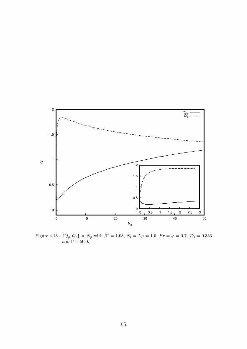
0
0.5
1
1.5
2
0 10 20 30 40 50
Q
Ng
QgQs
0
0.5
1
1.5
2
0 0.5 1 1.5 2 2.5 3
Figure 4.13 - {Qg, Qs} × Ng with β∗ = 1.08, Nl = LF = 1.0, Pr = ϕ = 0.7, TB = 0.333and Γ = 50.0.
65
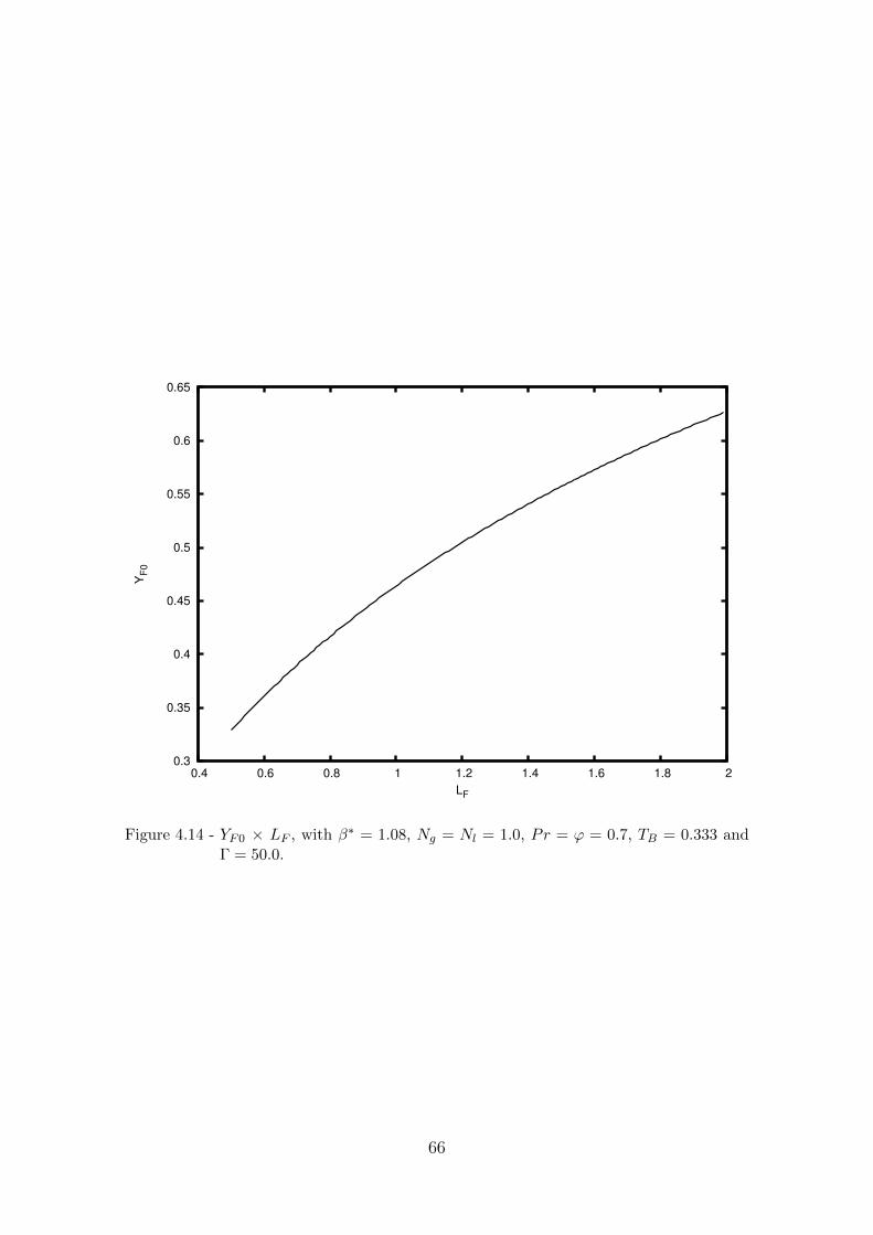
0.3
0.35
0.4
0.45
0.5
0.55
0.6
0.65
0.4 0.6 0.8 1 1.2 1.4 1.6 1.8 2
YF
0
LF
Figure 4.14 - YF0 × LF , with β∗ = 1.08, Ng = Nl = 1.0, Pr = ϕ = 0.7, TB = 0.333 andΓ = 50.0.
66
5 REACTIVE PROBLEM: DIFFUSION FLAME ESTABLISHED IN A
STAGNATION-POINT FLOW CONFIGURATION
In this Chapter we extend the previous Chapters by considering that the liquid
is a fuel and the impinging jet is an oxidant. A flame sheet is established in the
region where the mass fluxes are at stoichiometric proportion, inside the viscous
region around the plane that contains the stagnation-point. The exothermic reaction
releases heat, which is conducted to both sides of the flame sheet. In the fuel side,
this heat is used to vaporize the liquid fuel, a process that supplies the necessary
vapor to sustain the diffusion flame.
For liquid fuels, it has been shown that porous medium burner have some advan-
tages over the conventional spray systems (MUJEEBU et al., 2009). The intense radi-
ation field generated by the heated solid enhances the evaporation of fuel droplets
in the confined medium. For situations such that the droplets vaporize and mix
with oxidant prior to the combustion zone (MARTYNENKO et al., 1998; KAYAL;
CHAKRAVARTY, 2005), essentially a premixed flame is established.
The burning of fuels in non-premixed configurations has not received large atten-
tion, which can be measured by the small number of studies found in the literature.
However, potentially low emissions of NOx and CO for the burning of liquid fu-
els have been addressed (HOWELL et al., 1996). Hence, the study of non-premixed
flames in porous media deserves some attention. The evaporation and combustion of
ethanol from a porous surface when subjected to a boundary-layer-type flow of air
were studied experimentally (BOYARSHINOV et al., 1994). It has been found that the
flow velocity has a considerable effect on the flame temperature and the distribution
of mass flows over the wall. Also, heat and mass transfer coefficients decreased in
combustion. In addition, a similar boundary-layer-type reactive flow was considered
in analytical and numerical studies (LIU et al., 2008). The developed analytical model
investigates the dynamics of non-premixed flames in a shear layer established be-
tween a mainstream flow of fuel-rich combustion products and a porous surface with
an angled injection of air. The results were compared with numerical simulations
and a qualitative agreement in the surface temperature was observed. Furthermore,
comparison of the stability limits predicted by the model with the experimental data
was performed and a good qualitative agreement was obtained.
The problem of a free-convective diffusive flame in a porous media was also analyzed
by Chao et al. (1994). A similarity solution was considered in the infinitely thin
flame sheet limit of the reaction of a condensed fuel with an oxidizer flow driven by
67
the buoyancy force. The results showed that the temperature and species profiles
are qualitatively similar to those of the conventional, non-confined, free convection
flow. However, the flame temperature is lower as a result of a high value for the
effective Lewis number. This elevation on the effective Lewis number causes the
flame to moves towards the wall. It was also shown that the velocity field may have
a maximum at the reaction sheet or two maxima depending upon the temperature
dependence of the flow viscosity.
The specific case of stagnation-point diffusion flames stabilized next to a porous wick
was analyzed numerically by Raju and T’ien (2007). The porous wick was dipped
inside the liquid fuel reservoir and through capillary action the liquid is transported
to the surface of the wick and then evaporates and diffuses to the flame. Two regimes
beneath the flame, in the porous wick, were characterized: funicular and evaporative
regime. In the funicular regime a vapor-liquid (two-phase) region exists close to the
surface, with a single-phase liquid region below. In the evaporative regime there is
a single vapor phase above the two-phase region. It was shown that the funicular
regime was the only stable solution in the porous wick.
In the context of the in-situ combustion, Akkutlu and Yortsos (2003) studied the
conditions in which the flame propagation in a porous reservoir is stable. They have
considered weak heat losses to the ambient and derived expressions for temperature
and concentration profiles and the velocity of the combustion front, under both
adiabatic and non-adiabatic conditions. A coefficient that express the effective heat
transfer was obtained in terms of the reservoir thickness and front propagation speed.
Mailybaev et al. (2011) analyzed the in-situ combustion of oil with pyrolysis and
vaporization. By considering injection of air into a porous medium filled with inert
gas, medium or high viscosity oil and water, they analyzed the one-dimensional flow
generated by a combustion wave. Three pseudo-components were distinguished in the
oil: asphaltenes, medium and light oil. At high temperatures, the heavy components
were converted to coke, which undergoes combustion. The medium components of
the oil cracks and releases gaseous oil, while the light components and water are
vaporized. They considered that the condense phase was fixed in the reservoir and
analyzed the global problem of the propagating combustion front, then they obtained
solutions as a series of traveling waves.
The analysis of the in-situ combustion phenomenon through the propagating com-
bustion wave neglects diffusion as the analysis is focused on the global aspects of the
front. In those cases, the condensed fuel is considered to be at a fixed position inside
68
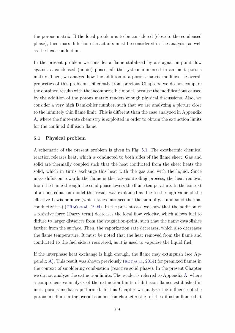
the porous matrix. If the local problem is to be considered (close to the condensed
phase), then mass diffusion of reactants must be considered in the analysis, as well
as the heat conduction.
In the present problem we consider a flame stabilized by a stagnation-point flow
against a condensed (liquid) phase, all the system immersed in an inert porous
matrix. Then, we analyze how the addition of a porous matrix modifies the overall
properties of this problem. Differently from previous Chapters, we do not compare
the obtained results with the incompressible model, because the modifications caused
by the addition of the porous matrix renders enough physical discussions. Also, we
consider a very high Damkohler number, such that we are analyzing a picture close
to the infinitely thin flame limit. This is different than the case analyzed in Appendix
A, where the finite-rate chemistry is exploited in order to obtain the extinction limits
for the confined diffusion flame.
5.1 Physical problem
A schematic of the present problem is given in Fig. 5.1. The exothermic chemical
reaction releases heat, which is conducted to both sides of the flame sheet. Gas and
solid are thermally coupled such that the heat conducted from the sheet heats the
solid, which in turns exchange this heat with the gas and with the liquid. Since
mass diffusion towards the flame is the rate-controlling process, the heat removal
from the flame through the solid phase lowers the flame temperature. In the context
of an one-equation model this result was explained as due to the high value of the
effective Lewis number (which takes into account the sum of gas and solid thermal
conductivities) (CHAO et al., 1994). In the present case we show that the addition of
a resistive force (Darcy term) decreases the local flow velocity, which allows fuel to
diffuse to larger distances from the stagnation-point, such that the flame establishes
farther from the surface. Then, the vaporization rate decreases, which also decreases
the flame temperature. It must be noted that the heat removed from the flame and
conducted to the fuel side is recovered, as it is used to vaporize the liquid fuel.
If the interphase heat exchange is high enough, the flame may extinguish (see Ap-
pendix A). This result was shown previously (ROY et al., 2014) for premixed flames in
the context of smoldering combustion (reactive solid phase). In the present Chapter
we do not analyze the extinction limits. The reader is referred to Appendix A, where
a comprehensive analysis of the extinction limits of diffusion flames established in
inert porous media is performed. In this Chapter we analyze the influence of the
porous medium in the overall combustion characteristics of the diffusion flame that
69
is generated by the stagnation-point flow against the condensed (liquid) phase.
Figure 5.1 - Schematic of the present problem.
The expressions for the solid temperature at the surface Ts0, vaporization rate m and
fuel mass fraction at the surface YF0 are the same as the ones obtained for the pure
vaporization case, given by Eqs. 4.16, 4.17 and 4.19. However, in the present case
we have the existence of an additional heat source and reactants sink, namely the
flame. This new heat source enhances the gas temperature, which by consequence
enhances the solid temperature because they are thermally coupled. The increase of
the temperature in the gas and solid phases enhances the vaporization rate because
of the higher value of the heat fluxes (gas and solid) towards the liquid-solid region
(recall that the vaporization rate is given by Eq. 4.17).
Thermal expansion enhances the local flow velocity, which increases the magnitude
of the Darcy resistance term (which is proportional to the local flow velocity, as
one can see from Eq. 2.42). Hence, at the flame this resistance is high (because
of the high local temperature, which by thermal expansion increases the local flow
velocity. Note that the Darcy resistance is effectively accounted by βT 2g ). If the
70
Darcy resistance is high enough, the flow decrease its local velocity at the flame,
rather than to increase it as in a non-confined problem. This makes the horizontal
flow velocity present a two-peak behavior, similar to the one reported by Chao et
al. (1994) in the context of a free-convective flame sheet established in an inert
porous media. If the Darcy resistance term is low enough, the flow resembles that
of the non-confined problem, with a local maximum horizontal velocity near the
flame and caused by gas acceleration due to the heat release at the flame sheet.
The Darcy term is proportional to the square of the local gas temperature T 2g and
to β ∼ [(1 − ϕ)/ϕ]2/(ad2p), such that its magnitude can be changed by considering
different values of the heat of combustion q (which modifies the flame temperature),
strain-rate a, medium porosity ϕ and particle sizes dp (which modify β).
5.2 Mathematical formulation
The full mathematical formulation derived in Chapter 2 is considered now. Then,
for the gas-solid region η > 0 the governing equations are given by
Prd3f
dη3+ f
d2f
dη2−(df
dη
)2
− βT 2g
df
dη= −Tg (1 + β) , (5.1)
Prd2(fTg)
dη2+ f
d(fTg)
dη− βT 3
g f = (1− β)dF
dη, (5.2)
− f dYFdη− ϕ
LF
d2YFdη2
= −ϕDaYFYOe−Ta/Tg , (5.3)
− f dYOdη− ϕ
LO
d2YOdη2
= −ϕφDaYFYOe−Ta/Tg , (5.4)
− f dTgdη− ϕd
2Tgdη2
= ϕqDaYFYOe−Ta/Tg + TgNg (Ts − Tg) , (5.5)
− Γ(1− ϕ)d
dη
(1
Tg
dTsdη
)= −TgNg (Ts − Tg) . (5.6)
For the liquid-solid region z < 0, we have
− Γ(1− ϕ)d2Tsdz2
= −Nl(Ts − TB). (5.7)
The boundary conditions are the same as the ones used in Chapter 4, but now we
must consider the additional boundary conditions for the oxidant mass fraction YO.
71
The boundary conditions for η →∞ are then given by
df
dη= 1, Ts = Tg = 1, YF = 0, YO = 1. (5.8)
At the surface η = 0, we have
df
dη= 0, Tg = TB, YO = 0. (5.9)
The relation between velocities at the interface and the liquid mass conservation
gives
− f(0) = m. (5.10)
The solid temperature at the surface Ts(0) > TB is an unknown to be obtained from
the continuity of the solid phase heat flux at the gas-liquid interface, given by
1
TB
dTsdη
∣∣∣∣0+
=dTsdz
∣∣∣∣0−. (5.11)
Reservoir condition, z → −∞, is given by
Ts = TB. (5.12)
At the interface η = z = 0, fuel mass fraction and energy conservation gives
ϕ
LF
dYFdη
∣∣∣∣0
= (1− YF0)f(0), (5.13)
ϕdTgdη
∣∣∣∣0+
+Nl
∫ 0−
−∞(Ts − TB)dz = m l TB. (5.14)
The solid phase temperature profile in the liquid-solid region is the same as the one
given by Eq. 4.15
Ts(z) = TB +
1
TB
dTsdη
∣∣∣∣0+
√Γ(1− ϕ)
Nl
e√Nl/(Γ(1−ϕ))z. (5.15)
The vaporization rate and the fuel mass fraction at the surface are also given by
Eqs. 4.17 and 4.19
m =T−1B
l
{ϕdTgdη
∣∣∣∣0+
+Γ(1− ϕ)
TB
dTsdη
∣∣∣∣0+
}, (5.16)
72
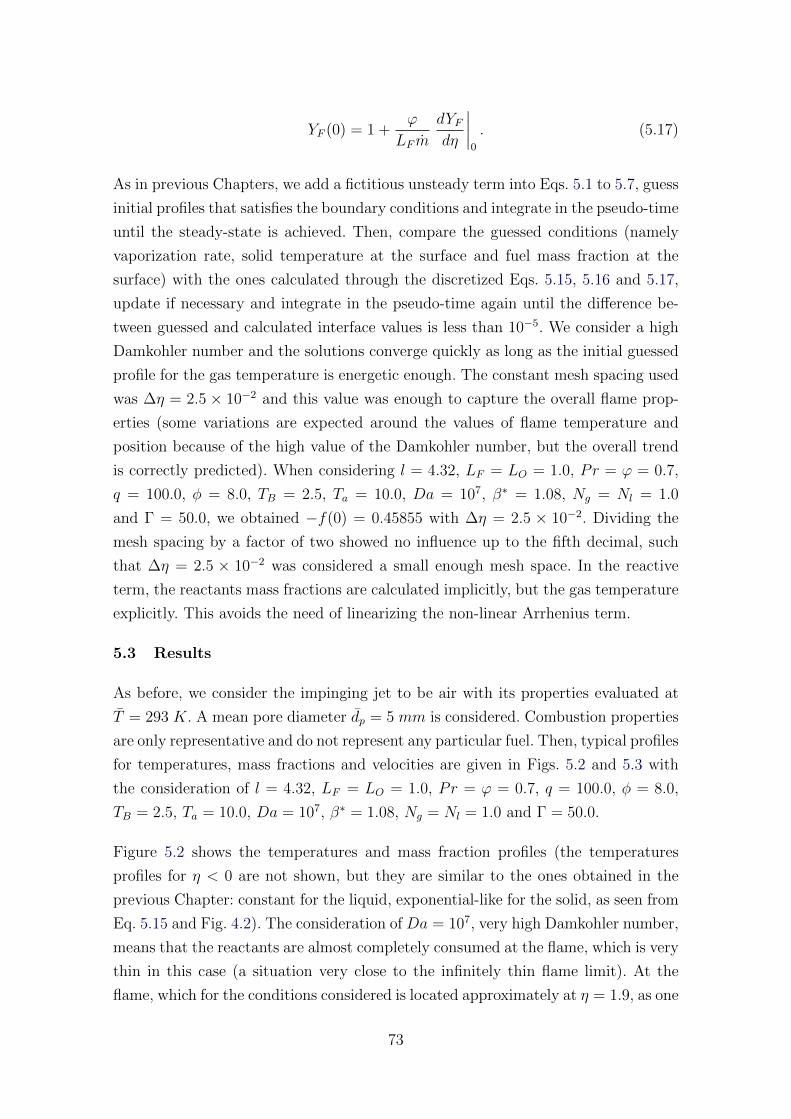
YF (0) = 1 +ϕ
LF m
dYFdη
∣∣∣∣0
. (5.17)
As in previous Chapters, we add a fictitious unsteady term into Eqs. 5.1 to 5.7, guess
initial profiles that satisfies the boundary conditions and integrate in the pseudo-time
until the steady-state is achieved. Then, compare the guessed conditions (namely
vaporization rate, solid temperature at the surface and fuel mass fraction at the
surface) with the ones calculated through the discretized Eqs. 5.15, 5.16 and 5.17,
update if necessary and integrate in the pseudo-time again until the difference be-
tween guessed and calculated interface values is less than 10−5. We consider a high
Damkohler number and the solutions converge quickly as long as the initial guessed
profile for the gas temperature is energetic enough. The constant mesh spacing used
was ∆η = 2.5 × 10⁻² and this value was enough to capture the overall flame prop-
erties (some variations are expected around the values of flame temperature and
position because of the high value of the Damkohler number, but the overall trend
is correctly predicted). When considering l = 4.32, LF = LO = 1.0, Pr = ϕ = 0.7,
q = 100.0, φ = 8.0, TB = 2.5, Ta = 10.0, Da = 107, β∗ = 1.08, Ng = Nl = 1.0
and Γ = 50.0, we obtained −f(0) = 0.45855 with ∆η = 2.5 × 10⁻². Dividing the
mesh spacing by a factor of two showed no influence up to the fifth decimal, such
that ∆η = 2.5 × 10⁻² was considered a small enough mesh space. In the reactive
term, the reactants mass fractions are calculated implicitly, but the gas temperature
explicitly. This avoids the need of linearizing the non-linear Arrhenius term.
5.3 Results
As before, we consider the impinging jet to be air with its properties evaluated at
T = 293 K. A mean pore diameter dp = 5 mm is considered. Combustion properties
are only representative and do not represent any particular fuel. Then, typical profiles
for temperatures, mass fractions and velocities are given in Figs. 5.2 and 5.3 with
the consideration of l = 4.32, LF = LO = 1.0, Pr = ϕ = 0.7, q = 100.0, φ = 8.0,
TB = 2.5, Ta = 10.0, Da = 107, β∗ = 1.08, Ng = Nl = 1.0 and Γ = 50.0.
Figure 5.2 shows the temperatures and mass fraction profiles (the temperatures
profiles for η < 0 are not shown, but they are similar to the ones obtained in the
previous Chapter: constant for the liquid, exponential-like for the solid, as seen from
Eq. 5.15 and Fig. 4.2). The consideration of Da = 107, very high Damkohler number,
means that the reactants are almost completely consumed at the flame, which is very
thin in this case (a situation very close to the infinitely thin flame limit). At the
flame, which for the conditions considered is located approximately at η = 1.9, as one
73
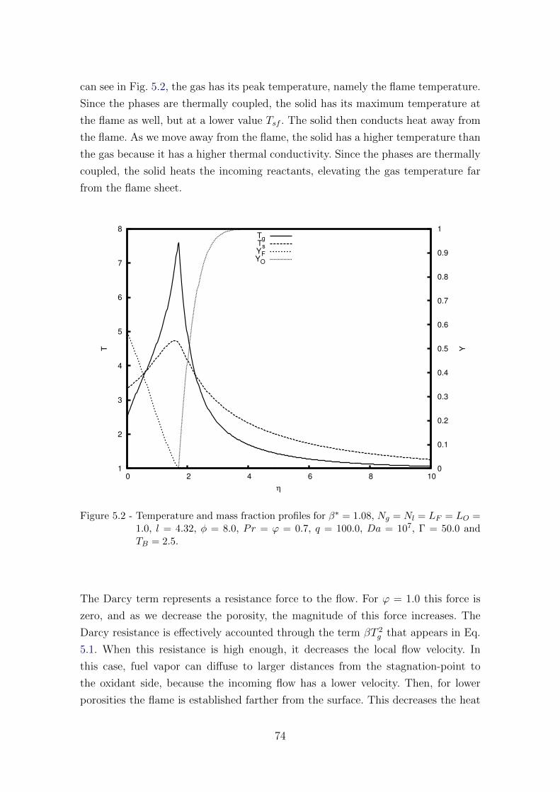
can see in Fig. 5.2, the gas has its peak temperature, namely the flame temperature.
Since the phases are thermally coupled, the solid has its maximum temperature at
the flame as well, but at a lower value Tsf . The solid then conducts heat away from
the flame. As we move away from the flame, the solid has a higher temperature than
the gas because it has a higher thermal conductivity. Since the phases are thermally
coupled, the solid heats the incoming reactants, elevating the gas temperature far
from the flame sheet.
1
2
3
4
5
6
7
8
0 2 4 6 8 10 0
0.1
0.2
0.3
0.4
0.5
0.6
0.7
0.8
0.9
1
T Y
η
TgTsYFYO
Figure 5.2 - Temperature and mass fraction profiles for β∗ = 1.08, Ng = Nl = LF = LO =1.0, l = 4.32, φ = 8.0, Pr = ϕ = 0.7, q = 100.0, Da = 107, Γ = 50.0 andTB = 2.5.
The Darcy term represents a resistance force to the flow. For ϕ = 1.0 this force is
zero, and as we decrease the porosity, the magnitude of this force increases. The
Darcy resistance is effectively accounted through the term βT 2g that appears in Eq.
5.1. When this resistance is high enough, it decreases the local flow velocity. In
this case, fuel vapor can diffuse to larger distances from the stagnation-point to
the oxidant side, because the incoming flow has a lower velocity. Then, for lower
porosities the flame is established farther from the surface. This decreases the heat
74
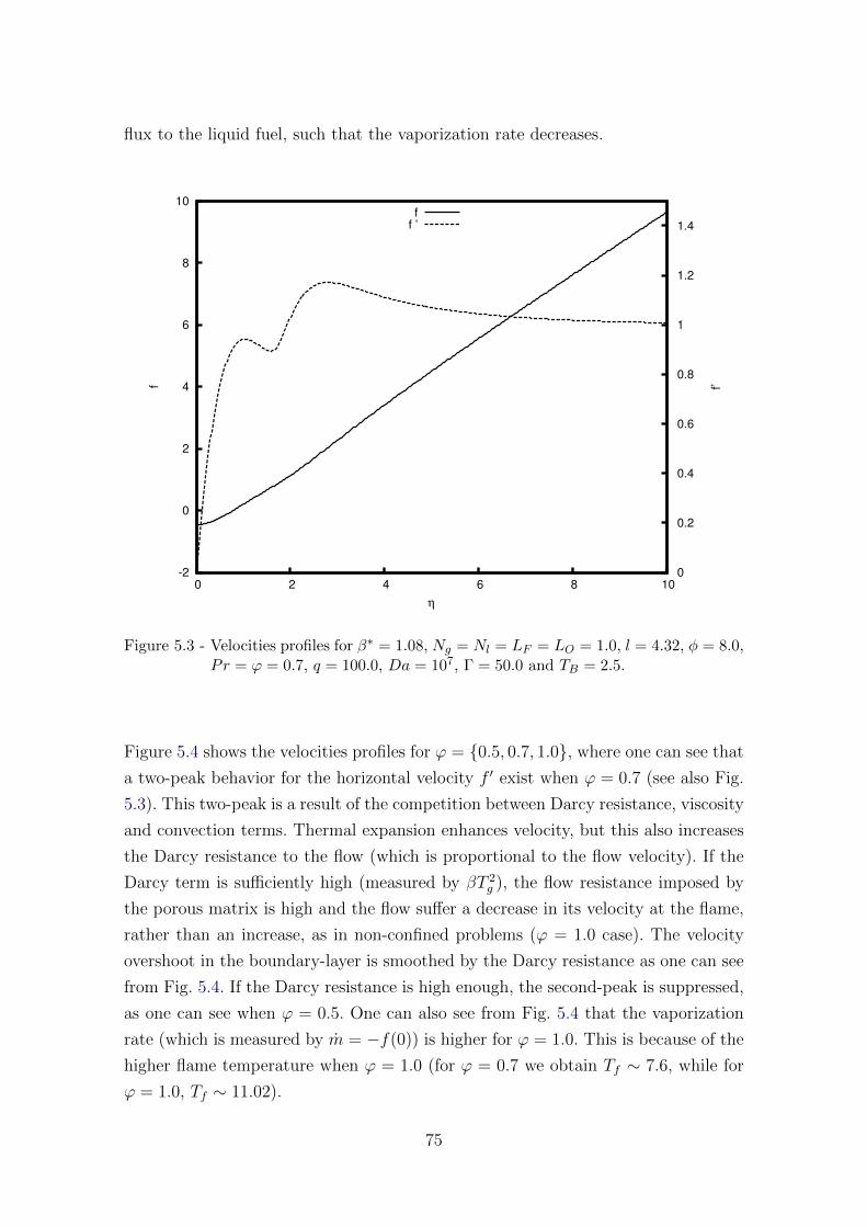
flux to the liquid fuel, such that the vaporization rate decreases.
-2
0
2
4
6
8
10
0 2 4 6 8 10 0
0.2
0.4
0.6
0.8
1
1.2
1.4
f f’
η
ff ’
Figure 5.3 - Velocities profiles for β∗ = 1.08, Ng = Nl = LF = LO = 1.0, l = 4.32, φ = 8.0,Pr = ϕ = 0.7, q = 100.0, Da = 107, Γ = 50.0 and TB = 2.5.
Figure 5.4 shows the velocities profiles for ϕ = {0.5, 0.7, 1.0}, where one can see that
a two-peak behavior for the horizontal velocity f ′ exist when ϕ = 0.7 (see also Fig.
5.3). This two-peak is a result of the competition between Darcy resistance, viscosity
and convection terms. Thermal expansion enhances velocity, but this also increases
the Darcy resistance to the flow (which is proportional to the flow velocity). If the
Darcy term is sufficiently high (measured by βT 2g ), the flow resistance imposed by
the porous matrix is high and the flow suffer a decrease in its velocity at the flame,
rather than an increase, as in non-confined problems (ϕ = 1.0 case). The velocity
overshoot in the boundary-layer is smoothed by the Darcy resistance as one can see
from Fig. 5.4. If the Darcy resistance is high enough, the second-peak is suppressed,
as one can see when ϕ = 0.5. One can also see from Fig. 5.4 that the vaporization
rate (which is measured by m = −f(0)) is higher for ϕ = 1.0. This is because of the
higher flame temperature when ϕ = 1.0 (for ϕ = 0.7 we obtain Tf ∼ 7.6, while for
ϕ = 1.0, Tf ∼ 11.02).
75
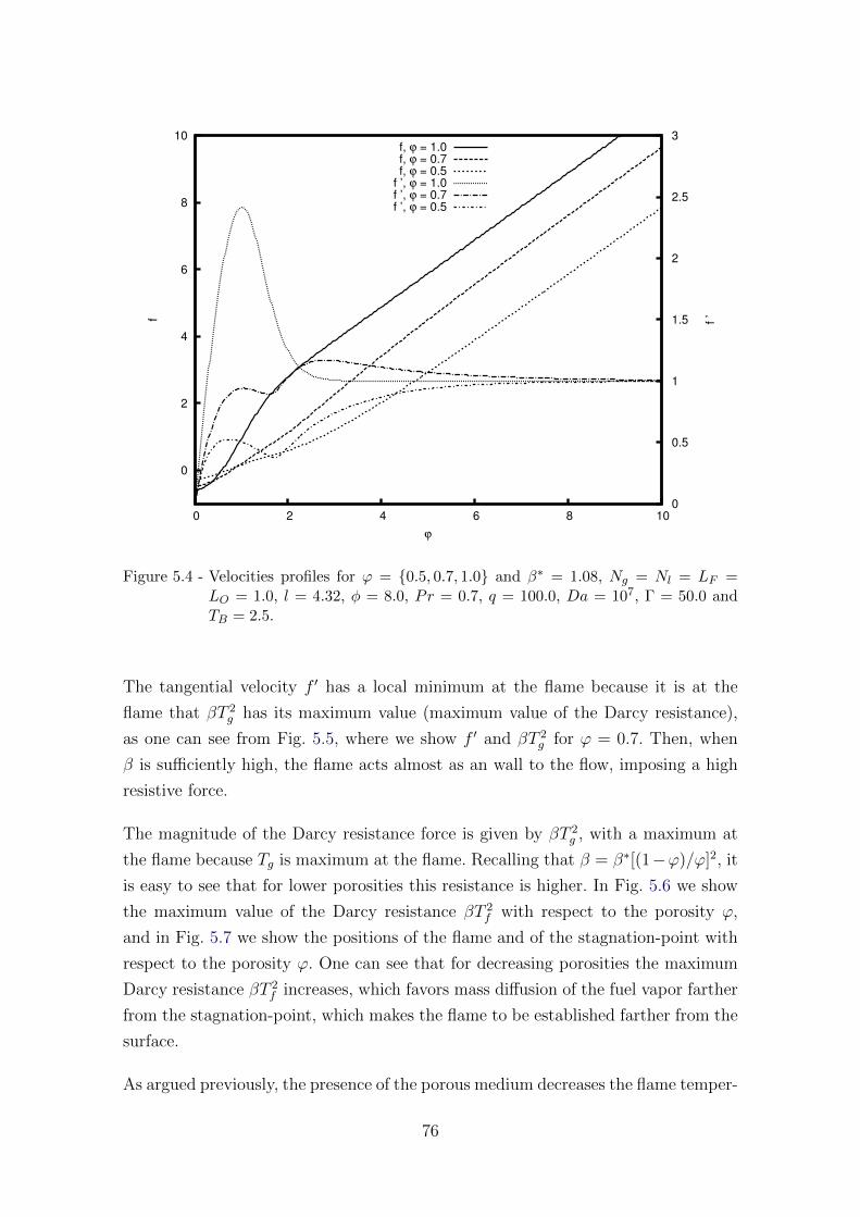
0
2
4
6
8
10
0 2 4 6 8 10 0
0.5
1
1.5
2
2.5
3
f f ’
ϕ
f, ϕ = 1.0f, ϕ = 0.7f, ϕ = 0.5
f ’, ϕ = 1.0f ’, ϕ = 0.7f ’, ϕ = 0.5
Figure 5.4 - Velocities profiles for ϕ = {0.5, 0.7, 1.0} and β∗ = 1.08, Ng = Nl = LF =LO = 1.0, l = 4.32, φ = 8.0, Pr = 0.7, q = 100.0, Da = 107, Γ = 50.0 andTB = 2.5.
The tangential velocity f ′ has a local minimum at the flame because it is at the
flame that βT 2g has its maximum value (maximum value of the Darcy resistance),
as one can see from Fig. 5.5, where we show f ′ and βT 2g for ϕ = 0.7. Then, when
β is sufficiently high, the flame acts almost as an wall to the flow, imposing a high
resistive force.
The magnitude of the Darcy resistance force is given by βT 2g , with a maximum at
the flame because Tg is maximum at the flame. Recalling that β = β∗[(1−ϕ)/ϕ]2, it
is easy to see that for lower porosities this resistance is higher. In Fig. 5.6 we show
the maximum value of the Darcy resistance βT 2f with respect to the porosity ϕ,
and in Fig. 5.7 we show the positions of the flame and of the stagnation-point with
respect to the porosity ϕ. One can see that for decreasing porosities the maximum
Darcy resistance βT 2f increases, which favors mass diffusion of the fuel vapor farther
from the stagnation-point, which makes the flame to be established farther from the
surface.
As argued previously, the presence of the porous medium decreases the flame temper-
76
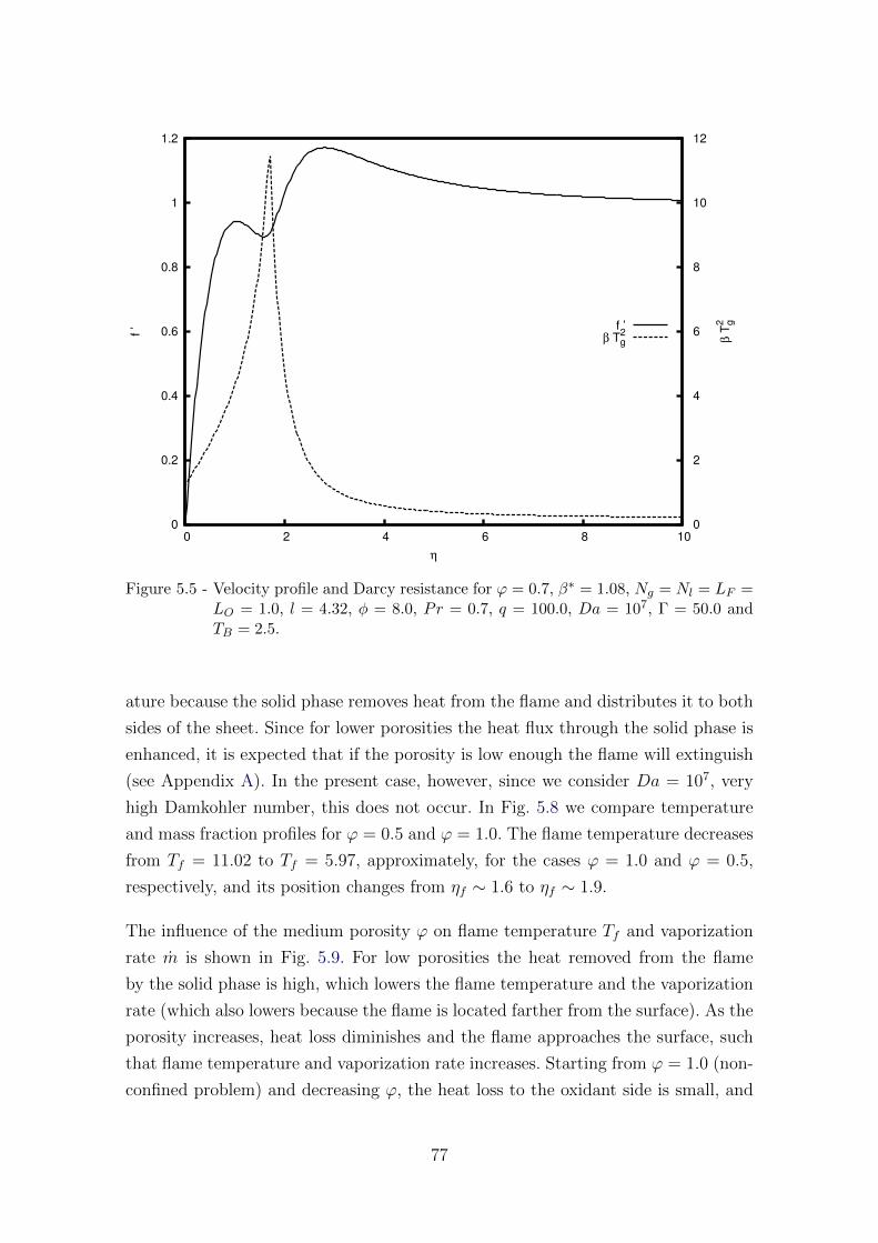
0
0.2
0.4
0.6
0.8
1
1.2
0 2 4 6 8 10 0
2
4
6
8
10
12f ’
β T
g2
η
f ’β Tg
2
Figure 5.5 - Velocity profile and Darcy resistance for ϕ = 0.7, β∗ = 1.08, Ng = Nl = LF =LO = 1.0, l = 4.32, φ = 8.0, Pr = 0.7, q = 100.0, Da = 107, Γ = 50.0 andTB = 2.5.
ature because the solid phase removes heat from the flame and distributes it to both
sides of the sheet. Since for lower porosities the heat flux through the solid phase is
enhanced, it is expected that if the porosity is low enough the flame will extinguish
(see Appendix A). In the present case, however, since we consider Da = 107, very
high Damkohler number, this does not occur. In Fig. 5.8 we compare temperature
and mass fraction profiles for ϕ = 0.5 and ϕ = 1.0. The flame temperature decreases
from Tf = 11.02 to Tf = 5.97, approximately, for the cases ϕ = 1.0 and ϕ = 0.5,
respectively, and its position changes from ηf ∼ 1.6 to ηf ∼ 1.9.
The influence of the medium porosity ϕ on flame temperature Tf and vaporization
rate m is shown in Fig. 5.9. For low porosities the heat removed from the flame
by the solid phase is high, which lowers the flame temperature and the vaporization
rate (which also lowers because the flame is located farther from the surface). As the
porosity increases, heat loss diminishes and the flame approaches the surface, such
that flame temperature and vaporization rate increases. Starting from ϕ = 1.0 (non-
confined problem) and decreasing ϕ, the heat loss to the oxidant side is small, and
77
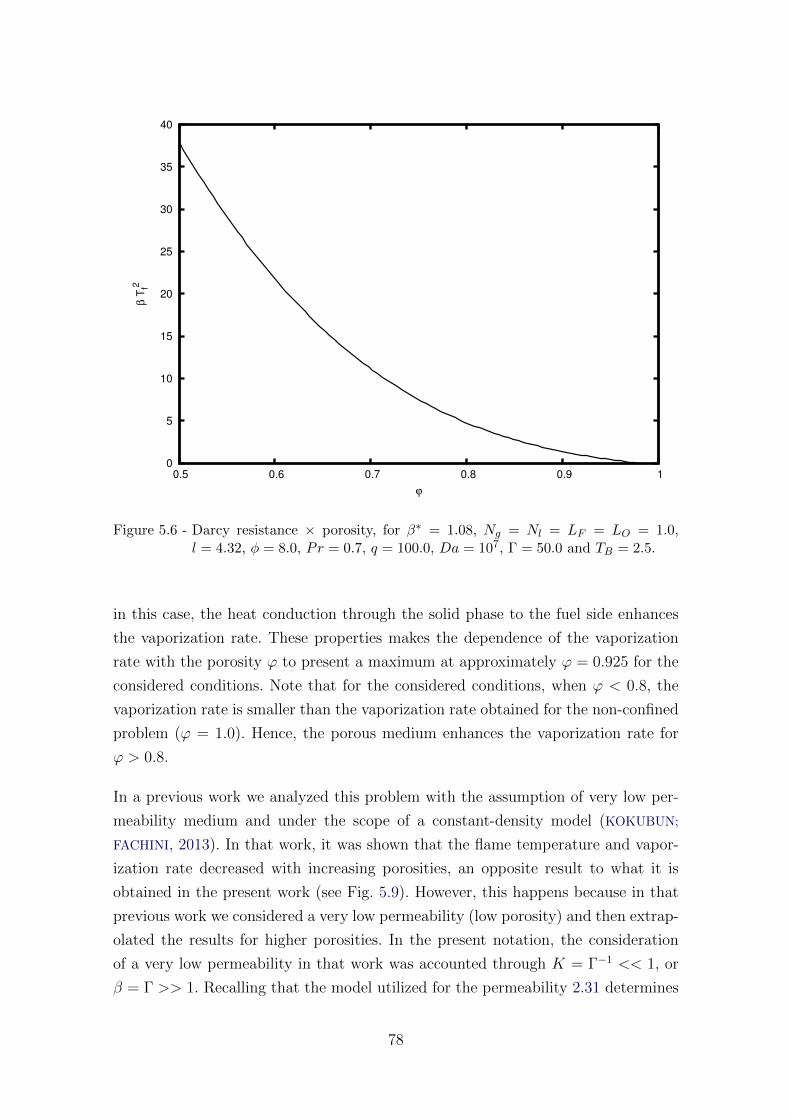
0
5
10
15
20
25
30
35
40
0.5 0.6 0.7 0.8 0.9 1
β T
f2
ϕ
Figure 5.6 - Darcy resistance × porosity, for β∗ = 1.08, Ng = Nl = LF = LO = 1.0,l = 4.32, φ = 8.0, Pr = 0.7, q = 100.0, Da = 107, Γ = 50.0 and TB = 2.5.
in this case, the heat conduction through the solid phase to the fuel side enhances
the vaporization rate. These properties makes the dependence of the vaporization
rate with the porosity ϕ to present a maximum at approximately ϕ = 0.925 for the
considered conditions. Note that for the considered conditions, when ϕ < 0.8, the
vaporization rate is smaller than the vaporization rate obtained for the non-confined
problem (ϕ = 1.0). Hence, the porous medium enhances the vaporization rate for
ϕ > 0.8.
In a previous work we analyzed this problem with the assumption of very low per-
meability medium and under the scope of a constant-density model (KOKUBUN;
FACHINI, 2013). In that work, it was shown that the flame temperature and vapor-
ization rate decreased with increasing porosities, an opposite result to what it is
obtained in the present work (see Fig. 5.9). However, this happens because in that
previous work we considered a very low permeability (low porosity) and then extrap-
olated the results for higher porosities. In the present notation, the consideration
of a very low permeability in that work was accounted through K = Γ−1 << 1, or
β = Γ >> 1. Recalling that the model utilized for the permeability 2.31 determines
78
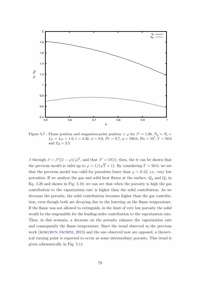
0.4
0.6
0.8
1
1.2
1.4
1.6
1.8
2
0.5 0.6 0.7 0.8 0.9 1
ηf ,
ηst
ϕ
ηfηst
Figure 5.7 - Flame position and stagnation-point position × ϕ for β∗ = 1.08, Ng = Nl =LF = LO = 1.0, l = 4.32, φ = 8.0, Pr = 0.7, q = 100.0, Da = 107, Γ = 50.0and TB = 2.5.
β through β = β∗[(1− ϕ)/ϕ]2, and that β∗ = O(1), then, the it can be shown that
the previous model is valid up to ϕ ∼ 1/(√
Γ + 1). By considering Γ = 50.0, we see
that the previous model was valid for porosities lower than ϕ ∼ 0.12, i.e., very low
porosities. If we analyze the gas and solid heat fluxes at the surface, Qg and Qs in
Eq. 4.20 and shown in Fig. 5.10, we can see that when the porosity is high the gas
contribution to the vaporization rate is higher than the solid contribution. As we
decrease the porosity, the solid contribution becomes higher than the gas contribu-
tion, even though both are decaying due to the lowering on the flame temperature.
If the flame was not allowed to extinguish, in the limit of very low porosity the solid
would be the responsible for the leading-order contribution to the vaporization rate.
Then, in this scenario, a decrease on the porosity enhance the vaporization rate
and consequently the flame temperature. Since the trend observed in the previous
work (KOKUBUN; FACHINI, 2013) and the one observed now are opposed, a theoret-
ical turning point is expected to occur at some intermediary porosity. This trend is
given schematically in Fig. 5.11.
79
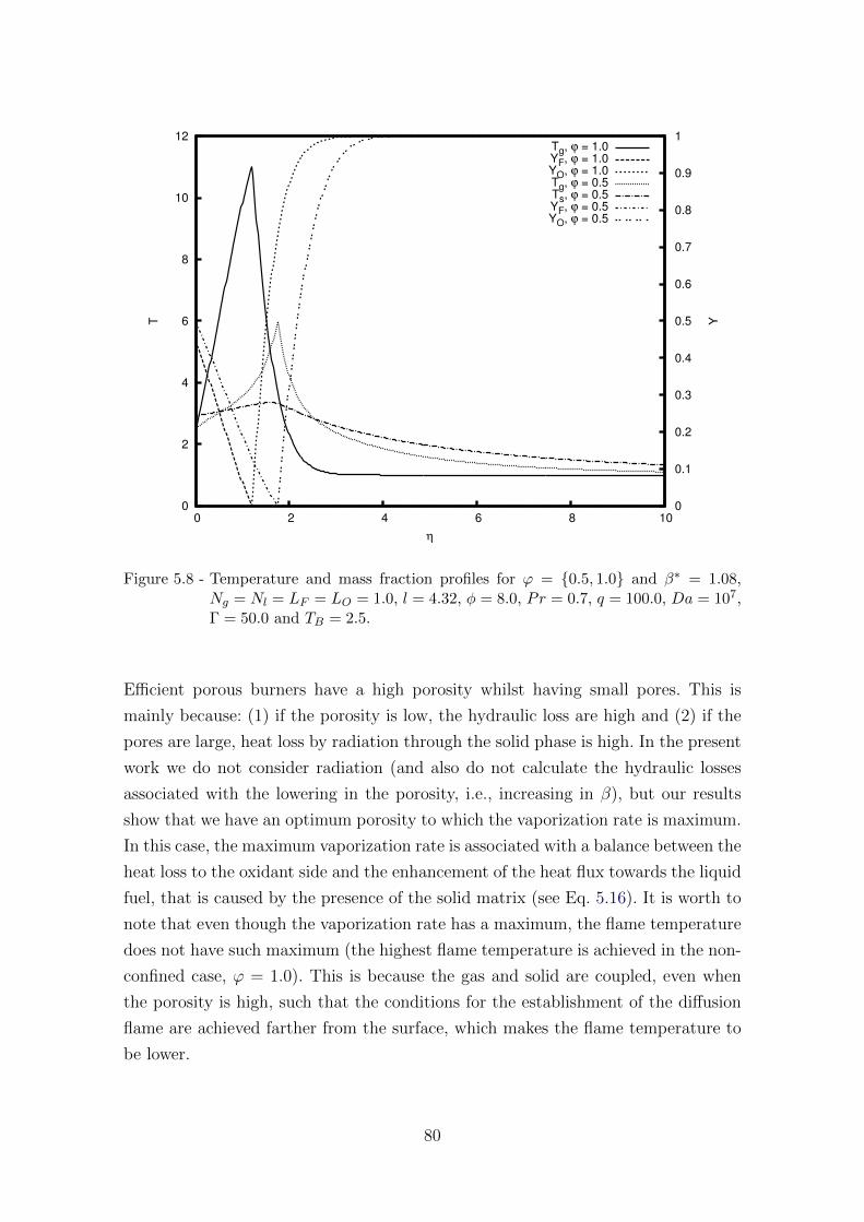
0
2
4
6
8
10
12
0 2 4 6 8 10 0
0.1
0.2
0.3
0.4
0.5
0.6
0.7
0.8
0.9
1
T Y
η
Tg, ϕ = 1.0YF, ϕ = 1.0YO, ϕ = 1.0Tg, ϕ = 0.5Ts, ϕ = 0.5YF, ϕ = 0.5YO, ϕ = 0.5
Figure 5.8 - Temperature and mass fraction profiles for ϕ = {0.5, 1.0} and β∗ = 1.08,Ng = Nl = LF = LO = 1.0, l = 4.32, φ = 8.0, Pr = 0.7, q = 100.0, Da = 107,Γ = 50.0 and TB = 2.5.
Efficient porous burners have a high porosity whilst having small pores. This is
mainly because: (1) if the porosity is low, the hydraulic loss are high and (2) if the
pores are large, heat loss by radiation through the solid phase is high. In the present
work we do not consider radiation (and also do not calculate the hydraulic losses
associated with the lowering in the porosity, i.e., increasing in β), but our results
show that we have an optimum porosity to which the vaporization rate is maximum.
In this case, the maximum vaporization rate is associated with a balance between the
heat loss to the oxidant side and the enhancement of the heat flux towards the liquid
fuel, that is caused by the presence of the solid matrix (see Eq. 5.16). It is worth to
note that even though the vaporization rate has a maximum, the flame temperature
does not have such maximum (the highest flame temperature is achieved in the non-
confined case, ϕ = 1.0). This is because the gas and solid are coupled, even when
the porosity is high, such that the conditions for the establishment of the diffusion
flame are achieved farther from the surface, which makes the flame temperature to
be lower.
80
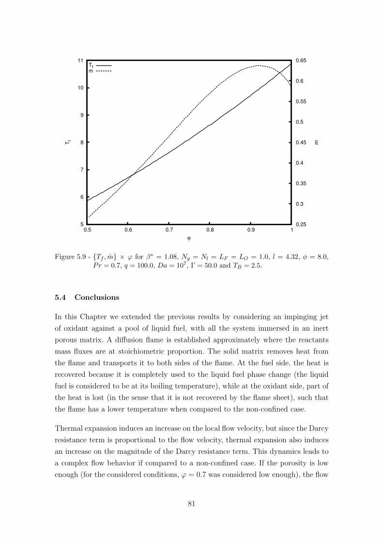
5
6
7
8
9
10
11
0.5 0.6 0.7 0.8 0.9 1 0.25
0.3
0.35
0.4
0.45
0.5
0.55
0.6
0.65
Tf
m
ϕ
Tfm
Figure 5.9 - {Tf , m} × ϕ for β∗ = 1.08, Ng = Nl = LF = LO = 1.0, l = 4.32, φ = 8.0,Pr = 0.7, q = 100.0, Da = 107, Γ = 50.0 and TB = 2.5.
5.4 Conclusions
In this Chapter we extended the previous results by considering an impinging jet
of oxidant against a pool of liquid fuel, with all the system immersed in an inert
porous matrix. A diffusion flame is established approximately where the reactants
mass fluxes are at stoichiometric proportion. The solid matrix removes heat from
the flame and transports it to both sides of the flame. At the fuel side, the heat is
recovered because it is completely used to the liquid fuel phase change (the liquid
fuel is considered to be at its boiling temperature), while at the oxidant side, part of
the heat is lost (in the sense that it is not recovered by the flame sheet), such that
the flame has a lower temperature when compared to the non-confined case.
Thermal expansion induces an increase on the local flow velocity, but since the Darcy
resistance term is proportional to the flow velocity, thermal expansion also induces
an increase on the magnitude of the Darcy resistance term. This dynamics leads to
a complex flow behavior if compared to a non-confined case. If the porosity is low
enough (for the considered conditions, ϕ = 0.7 was considered low enough), the flow
81
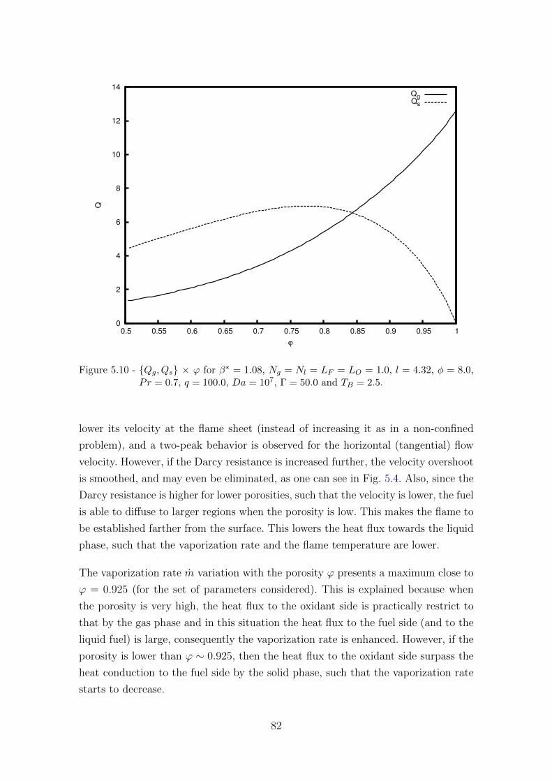
0
2
4
6
8
10
12
14
0.5 0.55 0.6 0.65 0.7 0.75 0.8 0.85 0.9 0.95 1
Q
ϕ
QgQs
Figure 5.10 - {Qg, Qs} × ϕ for β∗ = 1.08, Ng = Nl = LF = LO = 1.0, l = 4.32, φ = 8.0,Pr = 0.7, q = 100.0, Da = 107, Γ = 50.0 and TB = 2.5.
lower its velocity at the flame sheet (instead of increasing it as in a non-confined
problem), and a two-peak behavior is observed for the horizontal (tangential) flow
velocity. However, if the Darcy resistance is increased further, the velocity overshoot
is smoothed, and may even be eliminated, as one can see in Fig. 5.4. Also, since the
Darcy resistance is higher for lower porosities, such that the velocity is lower, the fuel
is able to diffuse to larger regions when the porosity is low. This makes the flame to
be established farther from the surface. This lowers the heat flux towards the liquid
phase, such that the vaporization rate and the flame temperature are lower.
The vaporization rate m variation with the porosity ϕ presents a maximum close to
ϕ = 0.925 (for the set of parameters considered). This is explained because when
the porosity is very high, the heat flux to the oxidant side is practically restrict to
that by the gas phase and in this situation the heat flux to the fuel side (and to the
liquid fuel) is large, consequently the vaporization rate is enhanced. However, if the
porosity is lower than ϕ ∼ 0.925, then the heat flux to the oxidant side surpass the
heat conduction to the fuel side by the solid phase, such that the vaporization rate
starts to decrease.
82
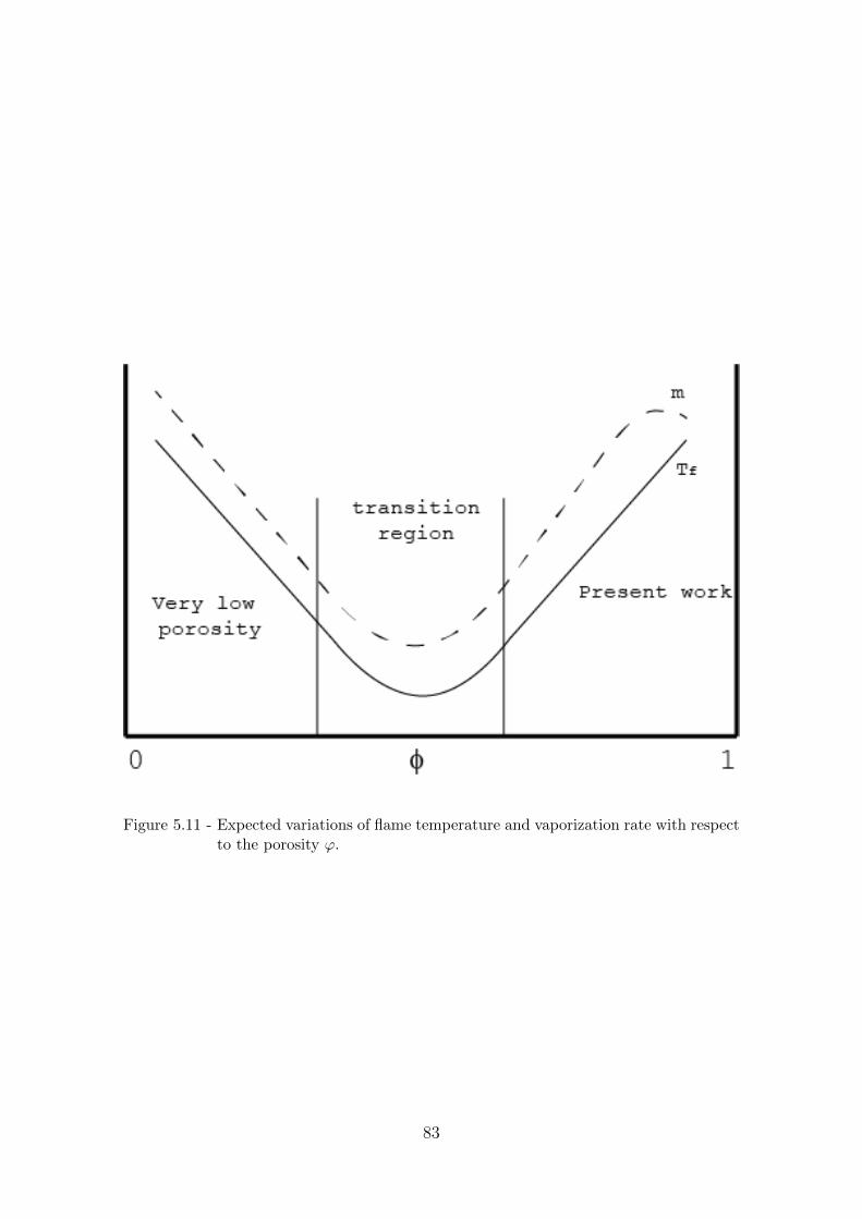
Figure 5.11 - Expected variations of flame temperature and vaporization rate with respectto the porosity ϕ.
83

6 CONCLUSIONS
In this work we analyzed a diffusion flame established inside an inert porous medium.
An impinging jet of oxidant against a liquid fuel pool, with all the system (gas and
liquid phases) immersed inside the porous matrix, was the considered geometry. A
semi-heuristic formulation was utilized, in which the Darcy term was added to the
usual compressible Navier-Stokes equations for the momentum components. The
thermal interaction between phases was accounted through an interphase heat ex-
change term, that couples gas and solid; and liquid and solid energy equations. In
order to obtain a better understanding of the physical features that occurr in such
system, we divided the problem in three parts.
In the first, we analyze a frozen impinging flow of gas against a hot impermeable
wall (the gas is confined in the porous matrix): heat transfer problem. The results
obtained, which are relevant for the study of porous heat exchangers, shows the
existence of velocity overshoot in the viscous boundary-layer, like in a non-confined
problem. However, if the porosity is low enough, the Darcy resistance to the flow
smooth this overshoot. The presence of the solid phase enhances heat transport to
large regions because the solid has a higher thermal conductivity compared to gas.
This increases the length of the thermal boundary-layer (a growth that is propor-
tional to√
Γ(1− ϕ), i.e., the square root of the product between the solid-to-gas
thermal conductivities ratio Γ and the solid volume (1−ϕ)). Comparing the obtained
results with results obtained for an incompressible model (constant density), it is
shown that thermal expansion usually enhances the wall shear. However, if the wall
temperature is high enough, the Darcy resistance term may be high (as it is mea-
sured by βT 2g ), which may lowers the local flow velocity, leading to a decrease on the
wall shear for high values of the wall temperature, a behavior not captured by incom-
pressible models (which measures the Darcy resistance only through β). Depending
on the value of β (inverse of the Darcy number, which is based on the viscous length-
scale), the pressure field may present a maximum above the stagnation-point due
to the high pore-level dissipation. The existence of a singular point for β = 1 might
point to the need of using a different model for the pressure when the permeability
is low (β > 1).
In the second part we replace the impermeable wall by a liquid pool and consider
that the incoming jet is hot, such that a vaporization problem was analyzed. In this
case, the heat and mass transfer properties in the confined problem were analyzed
by considering a frozen flow (chemical term set to zero). Velocity overshoot was
85
not observed because this demands the existence of a temperature in the viscous
boundary-layer higher than the free-stream temperature. The addition of a porous
matrix enhances heat transport towards the liquid, which increases the vaporization
rate. The consideration of thermal expansion leads to higher values of the vaporiza-
tion rate, solid temperature at the surface and vapor mass fraction at the surface.
Also, since the flow velocity is enhanced, vapor transport from the surface to above
the stagnation-point is more difficult. The liquid vaporization rate increases with
increasing values of the liquid-solid heat exchange coefficient Nl. In the asymptotic
limit of Nl � 1 the vaporization rate growth is proportional to√Nl. An increase on
the solid-to-gas thermal conductivities ration Γ also increases the vaporization rate
because it increases heat transport through the solid phase. For increasing values of
the gas-solid heat exchange coefficient Ng the vaporization rate increases. From Fig.
4.13 one can see that for small Ng the solid has a greater influence on the vaporiza-
tion rate than the gas. As Ng increases, the lowering on the temperatures difference
leads to the phases contributing more equally to the vaporization rate. Since the
solid has a much larger thermal conductivity than the solid, when Ng is small the
growth of the vaporization rate is much more prominent than the growth when Ng
is greater, as one can see from Fig. 4.12.
Finally, in the third part we consider the incoming jet to be oxidant and the liquid to
be fuel. The chemical reaction was then taken into account and a confined diffusion
flame was analyzed. The solid matrix removes heat from the flame and conducts it
to oxidant and fuel sides. For the fuel side, this heat is recovered because it is used
to vaporize the liquid fuel, which is at its boiling temperature. For the oxidant side,
part of this heat is lost (in the sense that it is not recovered at the flame sheet).
Then, the porous matrix lowers the temperature of the confined diffusion flame. The
increase of the Darcy resistance term when the porosity is low makes the flow velocity
decrease at the flame, which leads the flow to present a two-peak behavior, with a
local minimum at the flame. The lower local flow velocity due to the high Darcy
resistance also allows the fuel to diffuse to larger regions beyond the stagnation-
point, which makes the flame to establish farther from the surface. Even though
the flame temperature only decreases with decreasing porosities, the vaporization
rate presents a maximum with the porosity. This occur because when the porosity
is high, the heat transport to the fuel side is enhanced by the solid matrix, such
that the vaporization rate increases accordingly. However, if the porosity is lowered
enough, the heat loss to the oxidant side becomes more relevant, such that the
heat flux towards the liquid fuel diminishes, lowering the vaporization rate. The low
temperatures achieved for the confined diffusion flames makes this system to have
86
potentially lower emissions of pollutants.
In Appendix A we perform an asymptotic analysis of the extinction limits of a dif-
fusion flame established in a porous chamber, in order to clarify the influence of
the gas-solid heat exchange on the extinction behavior of such confined flame. It
was shown that low porosities may extinguish this flame because of the increase of
the heat exchange coefficient N . The reactant that is more consumed at extinction
depends on the injection velocity V (which modifies the interphase heat exchange
coefficient). When the extinction diagram is shown with respect to the dimensionless
injection velocity, we can see that two extinction points exist: one for low injection
velocities and the other for high injection velocities. The extinction point associated
with the high injection velocity is the usual kinetic extinction point, which is associ-
ated with a low residence time of the reactants in the reaction region. The extinction
point associated with the low injection velocity is associated with a high value of the
heat loss (heat exchange between gas and solid phases). This low-velocity extinction
point was already observed previously in the literature (MATALON et al., 1979; MAT-
ALON; LUDFORD, 1979; TIEN, 1986; SIBULKIN, 1988; CHAO et al., 1990; CHAO; LAW,
1993; WANG et al., 2007), but differently from those cases, the Damkohler number
for the low-velocity extinction point is low, instead of high. This occur because the
injection velocity modifies the Burke-Schumann solutions in this confined problem,
as it changes the interphase heat exchange coefficient N , which modifies the stoichio-
metric flame temperature T sf (temperature associated with complete combustion).
If the heat exchange is high enough, namely N = O(ε−1) (where ε� 1 is the inverse
of the dimensionless activation energy), then the interphase heat exchange becomes
important in the reaction region. In this case, the leakage of reactants through the
flame sheet become of order of unity and the flame will fall into Linan’s premixed
flame regime (LINAN, 1974), such that a different asymptotic treatment is required.
6.1 Future works
Even though we attempted to cover a wide range of physical situations when we
divided the problem into three distinct, but closely related, parts, some simplifica-
tions that were considered when constructing the mathematical model deserve some
attention.
The consideration of constant interphase heat exchange coefficients Ng and Nl is
not realistic. These coefficients have no closed-form expression, but instead their
expressions rely on empirical correlations (in Appendix A we utilize one of such
correlations). For increasing flow velocities, these coefficients decrease, because the
87
higher contact time between fluid and solid decreases the heat exchange between
phases. This is expected to have a significant influence in the gas-solid region, which
have a complex flow profile. Also, if the pores are large, the Rosseland approxima-
tion fails and one must take into consideration heat transfer by radiation through
the solid phase. This will have a significant effect on the vaporization rate and on
the flame temperature. In the realistic case where a three-phase region below the
interface exists, the formation of bubbles at the pore walls decrease the local heat
transfer between solid and liquid, which will decrease the vaporization rate. Then,
the consideration of a constant-temperature, two-phase zone in which the liquid fuel
undergoes phase change overpredicts the vaporization rate. If the heat transfer is
intense, there is a dramatic reduction in the vaporization rate (ZHAO; LIAO, 2000).
For diffusion flames, the rate-controlling process is the mass diffusion of reactants
towards the flame sheet. Then, the pre-heating of the reactants caused by the solid
phase should be significant only if the mass diffusion of reactants towards the flame
increases. Since we consider ρ2Di = 1, this effect is minimum (if not completely
negligible). If we consider the more realistic case of ρ2Di ∼ T ag (where a > 0), it is
expected that the pre-heating of the reactants becomes relevant, as it will influence
directly the mass diffusion of reactants towards the flame sheet. In this case, results
for the flame temperature will be higher than the ones obtained in the present work.
Nevertheless, the proposed model can shed some light into the heat and mass transfer
processes that occur in confined media. The work presented here form the basis
for future researches that can be performed. We anticipate some of the possible
extensions:
• Consideration of proper models for Ng and Nl, i.e., the interphase heat
exchange coefficients;
• Consideration of radiation through the solid-phase;
• More realistic temperature-dependences for the gas viscosity and for the
mass-diffusion coefficients;
• Proper modelling of the three-phase region right below the gas-liquid sur-
face (using the model developed by Raju and T’ien (2007) as basis, for
instance);
• Ignition conditions for the problem analyzed in Chapter 4;
• Extinction limits for the problem analyzed in Chapter 5.
88
REFERENCES
AKKUTLU, I. Y.; YORTSOS, Y. C. The dynamics of in-situ combustion fronts in
porous media. Combust. Flame, v. 134, p. 229–247, 2003. 1, 68
ALI, S. M. F. Heavy oil - evermore mobile. J. Petroleum Sci. Engng, v. 37,
p. 5–9, 2003. 1
ATTIA, H. On the effectiveness of porosity on stagnation point flow with heat
transfer over a permeable surface. J. Porous Media, v. 10, p. 625–631, 2007. 29
BARRA, A.; ELLZEY, J. Heat recirculation and heat transfer in porous burners.
Combust. Flame, v. 137, p. 230–241, 2004. 1
BOYARSHINOV, B. F.; VOLCHKOV, E. P.; TEREKHOV, V. I. Heat and mass
transfer in a boundary layer with the evaporation and combustion of ethanol.
Combust. Expl. Shock Waves, v. 30, p. 1–8, 1994. 67
BRANCH, M. C. In-situ combustion retorting of oil shale. Prog. En. Combust.
Sci., v. 5, p. 193–206, 1979. 1
CASTANIER, L. M.; BRIGHAM, W. E. Upgrading of crude oil via in situ
combustion. J. Petroleum Sci. Engng, v. 39, p. 125–136, 2003. 1
CHAO, B. H.; CHENG, P.; LE, T. Free-convective diffusion flame sheet in porous
media. Combust. Sci. Tech, v. 99, p. 37–41, 1994. 3, 5, 6, 16, 67, 69, 71
CHAO, B. H.; LAW, C. K. Asymptotic theory of flame extinction with surface
radiation. Combust. Flame, v. 92, p. 1–24, 1993. 9, 87, 119
CHAO, B. H.; LAW, C. K.; TIEN, J. S. Structure and extinction of diffusion
flames with flame radiation. Symposium (International) on Combustion,
v. 23, p. 523–531, 1990. 87, 119
CHEATHAM, S.; MATALON, M. A general asymptotic theory of diffusion flames
with application to cellular instability. J. Fluid Mech., v. 414, p. 105–144, 2000.
8, 100, 102, 112, 113, 120
COHEN, C. B.; RESHOTKO, E. Similar solutions for the compressible laminar
boundary layer with heat transfer and pressure gradient. Naca Technical
Report, n. 3325, 1955. 34
89
DAURELLE, J. V.; TOPIN, F.; OCCELLI, R. Modeling of coupled heat and mass
transfers with phase change in a porous medium: application to superheated steam
drying. Numer. Heat Transf. Part A, v. 33, p. 39–63, 1998. 47
DUVAL, F.; FICHOT, F.; QUINTARD, M. A local thermal non-equilibrium model
for two-phase flows with phase-change in porous media. Int. J. Heat Mass
Transf., v. 47, p. 613–639, 2004. 15
FU, X.; VISKANTA, R.; GORE, J. P. Measurement and correlation of volumetric
heat transfer coefficients of cellular ceramics. Exp. Thermal Fluid Sci., v. 17, p.
285–293, 1998. 104
HOWARTH, L. On the solution of the laminar Boundary-layer equations. Proc.
Roy. London A, v. 164, p. 547–579, 1938. 26, 32
HOWELL, J. R.; HALL, M. J.; ELLZEY, J. L. Combustion of hydrocarbon fuels
within porous inert media. Prog. En. Combust. Sci., v. 22, p. 121–145, 1996. 1,
67
IL´ICHEV, A. T.; TSYPKIN, G. G.; PRITCHARD, D.; RICHARDSON, C. N.
Instability of the salinity profile during the evaporation of saline groundwater. J.
Fluid Mech., v. 614, p. 87–104, 2008. 48
JABBOUR, C.; M, Q.; BERTIN, H.; ROBIN, M. Oil recovery by steam injection:
three-phase flow effects. J. Petroleum Sci. Engng, v. 16, p. 109–130, 1996. 48
JENG, T. M.; TZENG, S. C. Experimental study of forced convection in metallic
porous block subject to a confined slot jet. Int. J. Heat Mass Transf., v. 46, p.
1242–1250, 2007. 29
JUGJAI, S.; PHOTHIYA, C. Liquid fuels-fired porous combustor-heater. Fuel,
v. 86, p. 1062–1068, 2007. 16
JUGJAI, S.; PONGSAI, C. Liquid fuels-fired porous burner. Combust. Sci.
Tech, v. 179, p. 1823–1840, 2007. 3, 4, 16
JUJGAI, S.; POLMART, N. Enhancement of evaporation and combustion of liquid
fuels through porous media. Exp. Thermal Fluid Sci., v. 27, p. 901–909, 2003.
3, 4
JUJGAI, S.; WONGPANIT, N.; LAOKETKAN, T.; NOKKAEW, S. The
combustion of liquid fuels using a porous medium. Exp. Thermal Fluid Sci.,
v. 26, p. 15–23, 2002. 3, 4
90
KAKUTKINA, N. A. Some stability aspects of gas combustion in porous media.
Combust. Expl. Shock Waves, v. 41, p. 395–404, 2006. 2
KAMAL, M. M.; MOHAMAD, A. A. Development of a cylindrical porous-medium
burner. J. Porous Media, v. 9, p. 469–481, 2006. 4
KAVIANY, M. Principles of heat transfer in porous media. 2. ed. [S.l.]:
Springer, 1995. 13, 14, 15, 19
KAYAL, T. K.; CHAKRAVARTY, M. Combustion of liquid fuel inside inert
porous media: an analytical approach. Int. J. Heat Mass Transf., v. 48, p.
331–339, 2005. 3, 67
KOKUBUN, M. A. E.; FACHINI, F. F. An analytical approach for a Hiemenz flow
in a porous medium with heat exchange. Int. J. Heat Mass Transf., v. 54, p.
3613–3621, 2011. 8, 30, 36, 44
. Asymptotic analysis of a Hiemenz flow in a low-porosity medium with
phase change. J. Fluid Mech., v. 698, p. 185–210, 2012. 8, 49
. Flame sheet model for the burning of a low-volatility liquid fuel in a
low-permeability medium under low rates of strain. Combust. Flame, v. 160, p.
2783–2799, 2013. 8, 78, 79
KOKUBUN, M. A. E.; PEREIRA, F. M.; FACHINI, F. F. Analytical study of
stretched ultra-lean premixed flames within porous inert media. Proc. Combust.
Institute, v. 34, p. 839–845, 2013. 1, 16
KUKUCK, S.; MATALON, M. The onset of oscillations in diffusion flames.
Combust. Theory Modelling, v. 5, p. 217–240, 2001. 113
LAEVSKII, Y. M.; BABKIN, V. S. Stabilized gas combustion wave in an inert
porous medium. Combust. Expl. Shock Waves, v. 44, p. 502–508, 2008. 2
LEE, D.; VAFAI, K. Analytical characterization and conceptual assessment of
solid and fluid temperature differentials in porous media. Int. J. Heat Mass
Transf., v. 42, p. 423–435, 1999. 30
LEHMANN, P.; ASSOULINE, S.; OR, D. Characteristic length scales affecting
evaporative drying of porous media. Phys. Rev. E, v. 77, 2008. 48
LINAN, A. The asymptotic structure of counterflow diffusion flames for large
activation energies. Acta Astronautica, v. 1, p. 1007–1039, 1974. 87, 103, 120
91
LIU, S.; FOTACHE, C. G.; CHAO, B. H.; HAUTMAN, D. J.; OCHS, S. S.
Boundary layer modeling of reactive flow over a porous surface with angled
injection. Combust. Flame, v. 154, p. 378–386, 2008. 67
MAILYBAEV, A. A.; BRUINING, J.; MARCHESIN, D. Analysis of in situ
combustion of oil with pyrolysis and vaporization. Combust. Flame, v. 158, p.
1097–1108, 2011. 1, 68
MARTYNENKO, V. V.; ECHIGO, R.; YOSHIDA, H. Mathematical model of
self-sustaining combustion in inert porous medium with phase change under
complex heat transfer. Int. J. Heat Mass Transf., v. 41, p. 117–126, 1998. 3, 67
MATALON, M.; LUDFORD, G. S. S. Chambered diffusion flames for different
supply temperatures. Acta Astronautica, v. 6, p. 1377–1386, 1979. 9, 87, 118
MATALON, M.; LUDFORD, G. S. S.; BUCKMASTER, J. Diffusion flames in a
chamber. Acta Astronautica, v. 6, p. 943–959, 1979. 9, 87, 118
METZENER, P.; MATALON, M. Diffusive-thermal instabilities of diffusion flames:
onset of cells and oscillations. Combust. Theory Modelling, v. 10, p. 701–725,
2006. 113
MIN, D. K.; SHIN, H. D. Laminar premixed flame stabilized inside a honeycomb
ceramic. Int. J. Heat Mass Transf., v. 34, p. 341–356, 1991. 16
MITAL, R.; GORE, J. P.; VISKANTA, R. A Study of the Structure of Submerged
Reaction Zone in Porous Ceramic Radiant Burners. Combust. Flame, v. 111, p.
175–184, 1997. 4
MUJEEBU, M. A.; ABDULLAH, M. Z.; BAKAR, M. Z. A.; MOHAMAD, A. A.;
ABDULLAH, M. K. A review of investigations on liquid fuel combustion in porous
inert media. Prog. En. Combust. Sci., v. 35, p. 216–230, 2009. 67
MUJEEBU, M. A.; ABDULLAH, M. Z.; MOHAMAD, A.; BAKAR, M. A. Trends
in modelling of porous media combustion. Prog. En. Combust. Sci., v. 36, p.
627–650, 2010. 1
NARAYAN, K. A.; WALSH, B. W. An experimental investigation of hydrocarbon
recovery from a porous medium by continuous steam injection. Fuel, v. 67, p.
215–220, 1988. 48
92
PEREIRA, F.; OLIVEIRA, A.; FACHINI, F. Asymptotic analysis of stationary
adiabatic premixed flames in porous inert media. Combust. Flame, v. 156, p.
152–165, 2009. 2, 3, 16
. Theoretical analysis of ultra-lean premixed flames in porous inert media. J.
Fluid Mech., v. 657, p. 285–307, 2010. 1, 3, 16
PEREIRA, F. M. Estudo analıtico da estrutura de chamas adiabaticas
pre-misturadas em meios porosos inertes e desenvolvimento de um
modelo de curvas de nıvel para simulacoes numericas. PhD Thesis (PhD)
— Universidade Federal de Santa Catarina, 2009. 12, 14
PEREIRA, F. M.; OLIVEIRA, A. A. M.; FACHINI, F. F. Maximum
superadiabatic temperature for stabilized flames within porous inert media.
Combust. Flame, v. 158, p. 2283–2288, 2011. 3, 16
RADULESCU, M. I.; MAXWELL, B. M. The mechanism of detonation
attenuation by a porous medium and its subsequent re-initiation. J. Fluid Mech.,
v. 667, p. 96–134, 2011. 1
RAJU, M. P.; T’IEN, J. S. Heat and Mass Transports in a One-Dimensional
Porous Wick Driven by a Gas-Phase Diffusion Flame. J. Porous Media, v. 10, p.
327–342, 2007. 4, 5, 20, 68, 88
RAMESH, P. S.; TORRANCE, K. E. Boiling in a porous layer heated from below:
effects of natural convection and a moving liquid/two-phase interface. J. Fluid
Mech., v. 257, p. 289–309, 1993. 47
REES, D. A. S.; BASSOM, A. P.; SIDDHESHWAR, P. G. Local thermal
non-equilibrium effects arising from the injection of a hot fluid into a porous
medium. J. Fluid Mech., v. 594, p. 379–398, 2008. 47
ROY, N. C.; HOSSAIN, A.; NAKAMURA, Y. A universal model of opposed flow
combustion of solid fuel over an inert porous medium. Combust. Flame, v. 161,
p. 1645–1658, 2014. 2, 69
SCHLICHTING, H. Boundary-layer theory. New York: McGraw-Hill, 1968.
81–86 p. 22
SESHADRI, K.; HUMER, S.; SEISER, R. Activation-energy asymptotic theory of
autoignition of condensed hydrocarbon fuels in non-premixed flows with
comparison to experiment. Combust. Theory Modelling, v. 12, p. 831–855,
2008. 20
93
SIBULKIN, M. Free convection diffusion flames from burning solid fuels. Prog.
En. Combust. Sci., v. 14, p. 195–212, 1988. 87, 119
STELZNER, B.; KERAMIOTIS, C.; VOSS, S.; FOUNTI, M. A.; TRIMIS, D.
Analysis of the flame structure for lean methane-air combustion in porous inert
media by resolving the hydroxyl radical. Proc. Combust. Institute, In Press,
2014. 4
TAKENO, T.; SATO, K. An excess enthalpy flame theory. Combust. Sci. Tech.,
v. 20, p. 73–84, 1979. 1
TELENGATOR, A. M.; MARGOLIS, S. B.; WILLIAMS, F. A. Stability of
quasi-steady deflagrations in confined porous energetic materials. Combust. Sci.
Tech, v. 160, p. 259–315, 2000. 1
TIEN, J. S. Diffusion flame extinction at small stretch rates: the mechanism of
radiative loss. Combust. Flame, v. 65, p. 31–34, 1986. 87, 119
T’IEN, J. S.; SINGHAL, S. N.; HARROLD, D. P.; PRAHL, J. M. Combustion and
Extinction in the Stagnation-Point Boundary Layer of a Condensed Fuel.
Combust. Flame, v. 33, p. 55–68, 1978. 26
TSENG, C.; HOWELL, J. Combustion of liquid fuels in a porous radiant burner.
Combust. Sci. Tech., v. 112, p. 141–161, 1996. 3
VAFAI, K. Handbook of porous media. Boca Raton, FL: CRC Press, 2005.
607–645 p. 1, 15
VAFAI, K.; KIM, S. K. Analysis of surface enhancement by a porous substrate. J.
Heat Transfer, v. 112, p. 700–706, 1990. 29
VOGEL, B. J.; ELLZEY, J. L. Subadiabatic and superadiabatic performance of a
two-section porous burner. Combust. Sci. Tech, v. 177, p. 1323–1338, 2005. 16
WANG, H. Y.; CHEN, W. H.; LAW, C. K. Extinction of counterflow diffusion
flames with radiative heat loss and nonunity Lewis numbers. Combust. Flame,
v. 148, p. 100–116, 2007. 9, 87, 119
WEINBERG, F. Combustion temperatures: the future? Nature, v. 233, p.
239–241, 1971. 1
WHITAKER, S. The Forchheimer equation: a theoretical development. Transport
in Porous Media, v. 25, p. 27–61, 1996. 15
94
WILLIAMS, F. A. Combustion theory. 2. ed. [S.l.]: The Benjamin/Cummings
Publishing Company, 1985. 11
WOOD, S.; HARRIS, A. T. Porous burners for lean-burn applications. Prog. En.
Combust. Sci., v. 34, p. 667–684, 2008. 1, 16
WOODS, A. W. Liquid and vapour flow in superheated rock. Annu. Rev. Fluid
Mech., v. 31, p. 171–199, 1999. 47
WU, Q.; WEINBAUM, S.; ANDREOPOULOS, Y. Stagnation-point flows in a
porous medium. Chem. Engng Sci., v. 60, p. 123–134, 2005. 25, 37, 42, 43
YARIN, L. P.; SUKHOV, G. S. On filtration combustion reactor theory.
Combust. Sci. Tech., v. 84, p. 15–32, 1992. 2
YORTSOS, Y. C.; STUBOS, A. K. Phase change in porous media. Curr. Opin.
Colloid Interface Sci., v. 6, p. 208–216, 2001. 47
ZHAO, T. S. Coupled heat and mass transfer of a stagnation point flow in a
heated porous bed with liquid film evaporation. Int. J. Heat Mass Transf.,
v. 42, p. 861–872, 1999. 47
ZHAO, T. S.; LIAO, Q. On capillary-driven flow and phase-change heat transfer in
a porous structure heated by a finned surface: measurements and modeling. Int. J.
Heat Mass Transf., v. 43, p. 1141–1155, 2000. 5, 20, 21, 88
ZHDANOK, S.; KENNEDY, L. A.; KOESTER, G. Superadiabatic combustion of
methane air mixtures under filtration in a packed bed. Combust. Flame, v. 100,
p. 221–231, 1995. 2
95

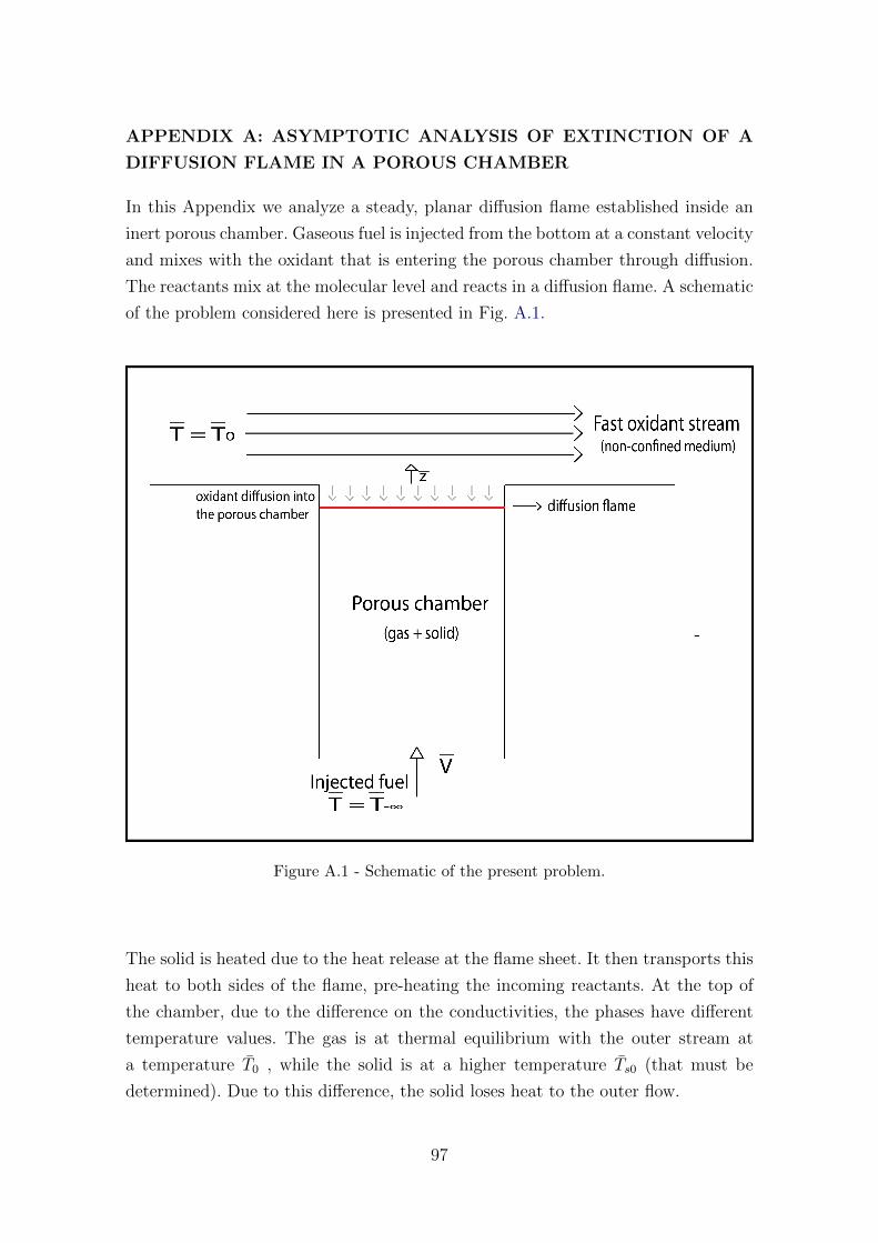
APPENDIX A: ASYMPTOTIC ANALYSIS OF EXTINCTION OF A
DIFFUSION FLAME IN A POROUS CHAMBER
In this Appendix we analyze a steady, planar diffusion flame established inside an
inert porous chamber. Gaseous fuel is injected from the bottom at a constant velocity
and mixes with the oxidant that is entering the porous chamber through diffusion.
The reactants mix at the molecular level and reacts in a diffusion flame. A schematic
of the problem considered here is presented in Fig. A.1.
Figure A.1 - Schematic of the present problem.
The solid is heated due to the heat release at the flame sheet. It then transports this
heat to both sides of the flame, pre-heating the incoming reactants. At the top of
the chamber, due to the difference on the conductivities, the phases have different
temperature values. The gas is at thermal equilibrium with the outer stream at
a temperature T0 , while the solid is at a higher temperature Ts0 (that must be
determined). Due to this difference, the solid loses heat to the outer flow.
97
We consider a single-step chemical reaction of the Arrhenius type. Due to the energy
generation in the gas phase we must consider a two-equation model for the gas-solid
system. The porous medium is considered isotropic and dispersion effects are ne-
glected, such that the effective thermal conductivities are order zero tensors. Hence,
the gas and solid conservation equations are coupled only through the interfacial
convective heat transfer coefficient h.
The major findings are related with the low flame temperatures achieved, when
compared to non-confined problems, and with the extinction limits. The extinction
diagram, when presented as a function of the injection velocity, shows the existence
of two distinct extinction points, one associated with a high velocity, and the other
associated with a low velocity. The high-injection-velocity extinction point is as-
sociated with kinetic extinction (low residence time for the reactants in the flame
sheet). The low-injection-velocity extinction point is associated with high values of
the interphase heat exchange.
It is interest to point that the existence of two extinction points was already rec-
ognized in the literature, and the low extinction point was associated with heat
losses with a high Damkohler number. In the present case, on the other hand, the
low extinction point (low injection velocity) is associated with a low value of the
Damkohler number. This occurs because the stoichiometric temperature is reduced
when the injection velocity is large (due to the enhancement of the interphase heat
exchange), which leads to a decrease on the reactive Damkohler number.
The results to be presented in the following were obtained in partnership with Pro-
fessor Moshe Matalon, from the University of Illinois at Urbana-Champaign.
A.1 Mathematical formulation
We consider a characteristic length1 given by ls = λs/(ρcpV ), with λs the thermal
conductivity of the solid, ρ the gas density, cp the gas specific heat capacity at
constant pressure and V the injection velocity of the gaseous fuel. Mass fractions
are non-dimensionalized with respect to their initial values YF−∞ and YO0 , for fuel
and oxidant, respectively. The temperatures are non-dimensionalized with respect
to q/cp , with q ≡ QYF−∞ being the heat released per unit mass of fuel.
The non-dimensional governing equations are then given by
1Note that the characteristic length scale given here is different than the one used in previousChapters.
98
dYFdz− 1
ΓLF
d2YFdz2
= −ΓDa YF YO e−Ta/Tg , (A.1)
dYOdz− 1
ΓLO
d2YOdz2
= −Γφ Da YF YO e−Ta/Tg , (A.2)
dTgdz− 1
Γ
d2Tgdz2
= Γ Da YF YO e−Ta/Tg + ΓN(Ts − Tg), (A.3)
− pd2Tsdz2
= −ΓN (Ts − Tg), (A.4)
where LF and LO are the fuel and oxidant Lewis numbers, respectively, φ ≡φYF−∞/YO0 is the initial mixture strength, Da ≡ BλgYO0/(cpV
2) is the Damkohler
number with B the frequency factor and we define N ≡ λgh/(ϕ(ρcpV )2) as the heat
exchange parameter and p ≡ (1−ϕ)/ϕ as the porosity parameter, with ϕ being the
porosity and h the volumetric surface-convection coefficient.
The non-dimensionalization process introduces the parameter Γ ≡ λs/λg, the solid-
to-gas thermal conductivities ratio. In this problem we consider the asymptotic limit
Γ � 1. Hence, one can see that we introduce a far-field length-scale, in which
convection is dominant and a region of the order of Γ−1 from the top of the chamber
in which convection and diffusion transport balance. Since in the convective, far-
field region, the solution for the oxidant mass fraction is given by YO = 0 (due
to the boundary condition for z → −∞), the chemical reaction is negligible in this
region. Chemical reaction occurs in the convective-diffusive region, which is analyzed
through the re-scaled spatial coordinate z = Γz. In the limit of very high porosity,
such that p = O(Γ−1) � 1, its easy to show that up to all orders Ts = Tg = T−∞
in the far-field. In this case, the consideration of the far-field length scale is not
necessary and we can simply analyze the problem in the usual viscous length scale
for non-confined problems (in this case, Γ−1ls). In Fig. A.2 we show a representative
picture of the profiles in each length-scale.
Boundary conditions for z → −∞ are given by
YF = 1, YO = 0, Ts = Tg = T−∞. (A.5)
For the top of the chamber z = 0,
YF = 0, YO = 1, Tg = T0, (A.6)
99
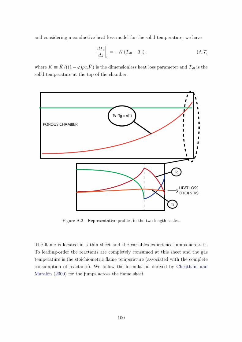
and considering a conductive heat loss model for the solid temperature, we have
dTsdz
∣∣∣∣0
= −K (Ts0 − T0) , (A.7)
where K ≡ K/((1−ϕ)ρcpV ) is the dimensionless heat loss parameter and Ts0 is the
solid temperature at the top of the chamber.
Figure A.2 - Representative profiles in the two length-scales.
The flame is located in a thin sheet and the variables experience jumps across it.
To leading-order the reactants are completely consumed at this sheet and the gas
temperature is the stoichiometric flame temperature (associated with the complete
consumption of reactants). We follow the formulation derived by Cheatham and
Matalon (2000) for the jumps across the flame sheet.
100
To leading-order the following jump relations must be satisfied across the flame sheet
[YF (0)
]=[YO(0)
]=[Tg(0)
]= 0,
[dTg(0)
dz
]= − 1
LF
[dYF (0)
dz
]= − 1
φLO
[dYO(0)
dz
],
(A.8)
in which [ F ] = F (z+f ) − F (z−f ) denotes the jump across the flame sheet which is
located at zf (z+f and z−f denotes the oxidant and fuel sides of the flame, respectively)
and F(0) is the leading-order term of the expansion F = F(0) + εF(1) + o(ε).
Also, complete combustion is required for the leading-order reactants, such that
YF (0)
∣∣zf
= YO(0)
∣∣zf
= 0. (A.9)
To O(ε) the the following jump relations must be satisfied across the flame
[Tg(1)
]= −L−1
F
[YF (1)
]= − (φLO)−1 [YO(1)
], (A.10)[
Tg(1) −dTg(1)
dz
]= −
[YF (1) − L−1
F
dYF (1)
dz
]= −
[YO(1) − (φLO)−1 dYO(1)
dz
], (A.11)
in which ε ≡ cpR(T sf)2/(qEa) is the inverse of the activation energy parameter,
with R the gas constant, Ea the activation energy and T sf the dimensional flame
temperature associated with complete combustion (or stoichiometric temperature).
For the solid phase, we must consider continuity of the temperature and its flux up
to all orders
[Ts] =
[dTsdz
]= 0. (A.12)
Leakage of reactants through the flame sheet is given by the higher-order terms,
such that
YF (1)(z+f ) = LF SF (γ, δ), YO(1)(z
−f ) = φ LO SO(γ, δ), (A.13)
where SF and SO are the fuel and oxidant leakage functions, respectively. This
leakage of reactants modifies the flame position. It is not so straight-forward to define
the correction for the flame position ηf . The first choice would be the point where
the temperature reach its peak, but in this case ηf must be determined numerically.
Then, if we define ηf as the point where the correction for the flame temperature is
continuous, we have [Tg(1)
]+ ηf
[dTg(0)
dz
]= 0, (A.14)
as the relation that defines the flame position correction ηf .
101
The auxiliary parameters that characterizes the internal flame structure are
γ ≡dTg(0)/dz
∣∣z+f
+ dTg(0)/dz∣∣z−f[
dTg(0)/dz] , δ ≡ 4φLFLO[
dTg(0)/dz]2 D exp
{1 + γ
2h∗O +
1− γ2
h∗F
},
(A.15)
where γ is a parameter that depends on the temperature profiles for complete com-
bustion and h∗O and h∗F are the excess/deficient enthalpy at the flame, given by
h∗O = T−f1 +1
φLOY −O , h∗F = T+
f1 +1
LFY +F , (A.16)
where Tf1 is the dimensionless correction of the flame temperature, which is ex-
panded as Tf = T sf + εTf1 + o(ε).
The modified (reactive) Damkohler number D is given by
D = ε3Da e−Ta/Tsf , (A.17)
where the usual distinguish limit of D = O(1) is considered for the asymptotic
analysis of the flame structure.
One can see that the excess enthalpy at the flame makes the relation between δ and
D non-trivial. For zero excess enthalpy at the flame they are directly proportional
to each other (a case that occurs for Li = 1 in an adiabatic, non-confined problem),
such that they represent the same physical state. In the present case, the excess
enthalpy at the flame is induced by non-unitary Lewis numbers and by the heat
exchange between gas and solid phases.
Cheatham and Matalon (2000) provided approximations for the leakage curves SF
and SO. For the lower branch (solutions that tend to the Burke-Schumann limit of
complete combustion when δ → +∞) we have
SO = a0 δ−4/3exp {−a1 (δ − δc)a2} , (A.18)
SF = b0 δ−4/3exp
{−b1 (δ − δc)b2
}, (A.19)
with
a0 = 0.61923 + 3.2523|γ|+ 0.52069|γ|2,
a1 = 1.9077− 1.901|γ|+ 1.055|γ|2,
a2 = 0.46137− 0.15374|γ| − 0.06769|γ|4 − 0.23288|γ|6,
102
b0 = 0.61923(1− |γ|)15exp {10.469|γ|} ,
b1 = 1.9077 + 11.588|γ|2 − 17.014|γ|4 + 55.865|γ|6,
b2 = 0.46137 + 0.27706|γ| − 0.2029|γ|2.
For the upper branch (solutions that corresponds to states with increasingly large
leakage of reactants and which become invalid when δ is sufficiently large)
SO = δ−1/3 {q0 + q1 (δ − δc)q2} , (A.20)
SF = δ−1/3 {r0 + r1 (δ − δc)r2} , (A.21)
q0 = 0.72704 (1− |γ|)−0.63858 exp{
1.4311|γ|0.5696},
q1 = 2.7108 +10.788tan (π|γ|/2)
1 + 2.5459|γ| − 2.8114|γ|2,
q2 = 0.625,
r0 = 0.72704 (1− |γ|)15 exp {10.451|γ|} ,
r1 = 2.7108 (1− |γ|)5.8507 ,
r2 = 0.625− 0.49221|γ|+ 2.0203|γ|2 − 4.2464|γ|3 + 4.2286|γ|4.
It is worth to note that the above approximations were obtained for −1 < γ ≤ 0,
which is the case when more heat is transported to the fuel side. When 0 ≤ γ < 1,
the roles of SF and SO must be interchanged.
In the above expressions, the critical δc was obtained by Linan (1974) and it is given
by
δc = e{
(1− |γ|)− (1− |γ|)2 + 0.26(1− |γ|)3 + 0.055(1− |γ|)4}. (A.22)
When N � 1, gas and solid temperature approach each other. In this case,
[dTg/dz] ∼ [dTs/dz] and it can be shown from the addition of Eqs. A.3 and A.4
that
γ = −[dT(0)
dz
](1 + Γp) . (A.23)
Then, unless p = O(Γ−1) (high-porosity) or[dT(0)/dz
]= O(Γ−1) (small heat re-
lease), γ will be large because Γ � 1. For |γ| > 1, there is O(1) reactant leakage
from the flame. Hence, when N � 1 the flame will fall into Linan’s premixed flame
regime (LINAN, 1974) and a different asymptotic treatment is required.
103
The dimensional heat exchange coefficient h is modeled following Fu et al. (1998)
and gives a dimensionless parameter N as
N = ϕ(m′−4)/2
(λgcp
)2C ′
µm′
(ρV
√4
π
1
39.37ϕ
)m′−2
, (A.24)
in which C ′ and m′ are experimentally-determined constants, µ is the gas-phase
kinematic viscosity and ϕ is the linear-pore density. Note that in this Appendix we
consider the correlations between the interphase heat exchange coefficient h, the
porosity ϕ and the flow velocity V , differently than in the previous Chapters. We
do so here because the flow field is trivial and given by the constant value V of the
injection velocity, and in the previous Chapters the flow field is more complex.
It is important to note that the formulation introduces two different perturbation
parameters, ε and Γ−1 , the first being associated with incomplete combustion and
leakage of reactants through the flame-sheet, and the second being associated with
the difference between gas and solid heat transport. For the sake of simplicity, we
analyze the distinguished limit of Γ−1 ∼ ε, such that we consider ε = cΓ−1 , with
c = O(1) being a proportionality constant.
A.2 Far-field, convective region
It is easy to show that mass fraction solutions in the far-field, convective region,
are simply given by YF (z) = 1 and YO(z) = 0 when the asymptotic limit of Γ � 1
is considered. Hence, chemical reaction is negligible in the convective region. Then,
one can manipulate energy equations and obtain
dTgdz− 1
Γ
d2Tgdz2− pd
2Tsdz2
= 0, (A.25)
− pd2Tsdz2
= −ΓN(Ts − Tg). (A.26)
One can see that the leading-order term for both phases is equal, as the heat exchange
term is dominant in the second equation. Hence, we expand gas and solid solutions
in series as
Ts(z) = T(0) + Γ−1Ts(1) + o(Γ−1), (A.27)
Tg(z) = T(0) + Γ−1Tg(1) + o(Γ−1), (A.28)
where we emphasize that the temperature difference arises only in the higher-order
terms.
104
Substituting the proposed solutions into the set of governing equations, we obtain
leading and higher-order equations as
dT(0)
dz− p
d2T(0)
dz2= 0, (A.29)
dTg(1)
dz−d2T(0)
dz2− p
d2Ts(1)
dz2= 0, (A.30)
− pd2T(0)
dz2= −N(Ts(1) − Tg(1)). (A.31)
Leading-order solution is given by
T(0)(z) = T−∞ + c0 ez/p, (A.32)
where c0 is a constant. If we integrate the higher-order equation for the gas-phase
and apply the result for z → −∞, we have the relation
Tg(1) = T ′(0) + pT ′s(1), (A.33)
where the prime denotes differentiation with respect to z. Substituting this in the
higher-order equation for the solid-phase we obtain
pT ′s(1) − Ts(1) = −c0
p
(1 +
1
N
)ez/p. (A.34)
Hence, the higher-order solution for the solid is given by
Ts(1)(z) = c1 ez/p − c0
(1 +
1
N
)z
p2ez/p, (A.35)
where c1 is a constant. Higher-order solution for the gas-phase is straight-forward
obtained as
Tg(1)(z) = c1 ez/p − c0
N pez/p − c0
(1 +
1
N
)z
p2ez/p. (A.36)
Then, temperature solutions in the convective region are given by
Tg(z) = T−∞ + c0 ez/p + Γ−1
{c1 e
z/p − c0
N pez/p − c0
(1 +
1
N
)z
p2ez/p}
+ o(Γ−1),
(A.37)
Ts(z) = T−∞ + c0 ez/p + Γ−1
{c1 e
z/p − c0
(1 +
1
N
)z
p2ez/p}
+ o(Γ−1). (A.38)
It is easy to see that when N � 1 (very intense interphase heat exchange), Ts → Tg,
while for p � 1 (very high porosity), {Ts, Tg} → T−∞. The unknown constants c0
105
and c1 are to be determined.
A.3 Convective-diffusive region
In a length scale of the order of Γ−1 close to z = 0, consumption of reactants is
observed, as it is in this region that convection and diffusion reactants transport
balance. Hence, in order to analyze this region we stretch the spatial coordinate as
z = Γz and obtain the following governing equations
dYFdz− 1
LF
d2YFdz2
= −Da YF YO e−Ta/Tg , (A.39)
dYOdz− 1
LO
d2YOdz2
= −φ Da YF YO e−Ta/Tg , (A.40)
dTgdz− d2Tg
dz2= Da YF YO e−Ta/Tg +N (Ts − Tg), (A.41)
− Γpd2Tsdz2
= −N(Ts − Tg). (A.42)
Boundary conditions for z = 0 are given by
Tg = Tg(0), YF = 0, YO = 1, ΓdTsdz
∣∣∣∣0
= −K (Ts(0)− Tg(0)) . (A.43)
We seek solutions in powers of ε = cΓ−1, or
YF (z) = YF (0) + εYF (1) + o(ε), (A.44)
YO(z) = YO(0) + εYO(1) + o(ε), (A.45)
Tg(z) = Tg(0) + εTg(1) + o(ε), (A.46)
Ts(z) = Ts(0) + εTs(1) + o(ε). (A.47)
For the mass fractions we have the following solutions (utilizing the boundary con-
106
ditions and jumps at the flame sheet shown previously)
YF (z) =
1− e(z−zf )LF
+
ε{
1 + SO/SF −{
LF /LO
φ+(1−φ)ezf LO
}(1−ezf LO
1−ezf LF
)}LF SF e(z−zf )LF , for z < zf
εLF SF(1− ezLF
)/(1− ezfLF
), for z > zf
,
(A.48)
YO(z) =
ε φ LO SO e(z−zf )LO , for z < zf
1−(
1−ezLO
1−ezf LO
)+ ε LF SF
φ
φ+(1−φ)ezf LO
(1−eLOz
1−eLOzf
)for z > zf .
.
(A.49)
Note that YF = O(ε) for z > zf and YO = O(ε) for z < zf , which denotes the small
leakage of reactants across the flame sheet.
Leading-order solution for the solid is given by
Ts(0)(z) = (c0 + T−∞), (A.50)
where matching with the far-field region was imposed.
Leading-order equation for the gas is given by
T ′g(0) − T ′′g(0) +N Tg(0) = N(c0 + T−∞). (A.51)
where prime denotes differentiation with respect to z. This equation must be solved
for both sides of the flame.
The general solution is given by
Tg(0)(z) = (c0 + T−∞) + ez/2(K1 e
Az/2 +K2 e−Az/2) , (A.52)
where A ≡√
4N + 1 comes from the characteristic equation of the homogeneous
solution.
For the fuel side, z < zf , matching with the far-field solution gives K−2 = 0. Then,
leading-order solution of the gas in the fuel side is given by
Tg(0)(z < zf ) = (c0 + T−∞) + c2 e(1+A)z/2, (A.53)
107
where c2 = K−1 is to be determined.
For the oxidant side, condition at the top of the chamber gives K+2 = −K+
1 −c0+∆T ,
where ∆T = T0−T−∞ is the temperature differential across the chamber. Then, we
have
Tg(0)(z > zf ) = (c0 + T−∞) + c3 e(1+A)z/2 − (c0 −∆T + c3) e(1−A)z/2, (A.54)
where K+1 = c3 is to be determined.
Higher-order equation for the solid is given by
c p T ′′s(1) +NTg(0) −N(c0 + T−∞) = 0. (A.55)
For the fuel side the following equation holds
c pd2Ts(1)
dz2+N c2 e
(1+A)z/2 = 0. (A.56)
Then, higher-order solution for the solid on the fuel side is given by
Ts(1)(z < zf ) =c0
c pz +
c1
c− 4N c2
c p(1 + A)2e(1+A)z/2, (A.57)
where matching with the far-field was imposed.
For the oxidant side, z > zf , we have the following governing equation
c pT ′′s(1) −N(c0 −∆T + c3) e(1−A)z/2 +N c3 e(1+A)z/2 = 0. (A.58)
General solution is given by
Ts(1)(z > zf ) = K+1 +K+
2 z +e(1−A)z/2
4Nc p
{(c0 −∆T + c3) (1 + A)2 − c3 e
Az(1− A)2}.
(A.59)
Up to leading-order the solid is at a constant temperature c0 + T−∞. At the top of
the chamber, we have Ts(0) = (c0 + T−∞) + Γ−1Ts1 + o(Γ−1). The correction of the
order of Γ−1 (Ts1) would have to be obtained from the heat loss condition at the
top of the chamber for the O(Γ−1) terms. For the present problem and discussion,
it is enough to consider Ts1 = 0, such that the condition at the top of the chamber
108
Ts(1)(0) = 0 determines
K+1 = − 1
4Ncp
{(c0 −∆T + c3)(1 + A)2 − c3(1− A)2
}, (A.60)
such that
Ts(1)(z > zf ) = K+2 z−
1
4Ncp
{(c0 −∆T + c3)(1 + A)2
(1− e(1−A)z/2
)− c3(1− A)2
(1− e(1+A)z/2
)}.
(A.61)
Applying the heat loss condition at the top of the chamber and collecting O(1)
terms, we have
cdTs(1)
dz
∣∣∣∣0
= −K(c0 −∆T ), (A.62)
which determines the constant K+2 in terms of c3 and c0 as
K+2 = −K
c(c0−∆t)− 1
4Ncp
{(c0 −∆T + c3)(1 + A)2 (1− A)
2− c3(1− A)2 (1 + A)
2
}.
(A.63)
Then we have the following solution
Ts(1)(z > zf ) = −Kc
(c0−∆T )z− 1
4Ncp
{(c0 −∆T + c3)(1 + A)2
(1− e(1−A)z/2 +
(1− A)z
2
)−
c3(1− A)2
(1− e(1+A)z/2 +
(1 + A)z
2
)}. (A.64)
Higher-order equation for the gas is given by
T ′g(1) − T ′′g(1) +NTg(1) = NTs(1), (A.65)
which must be solved for both sides of the flame.
For the fuel side we have the following governing equation
T ′g(1) − T ′′g(1) +NTg(1) = N
{c1
c+
c0
c pz − 4N c2
c p(1 + A)2e(1+A)z/2
}. (A.66)
109
General solution (discarding the exponentially large term) is given by
Tg(1)(z < zf ) = c4 e(1+A)z/2+
(c1
c− c0
Ncp+
c0
c pz
)+
4N2 c2
A2(1 + A)2c p(Az−1) e(1+A)z/2.
(A.67)
One can see that this solution matches properly with the far-field solution. The
integration constant c4 = K−1 is determined from the condition of continuity at the
flame (higher-order terms).
For the oxidant side, we have the following governing equation
T ′g(1) − T ′′g(1) +NTg(1) =
N
{−Kc
(c0 −∆T )z − 1
4Ncp
{(c0 −∆T + c3)(1 + A)2
(1− e(1−A)z/2 +
(1− A)z
2
)−
c3(1− A)2
(1− e(1+A)z/2 +
(1 + A)z
2
)}}. (A.68)
For the sake of compactness, we express the above in a general equation of the form
T ′g(1) − T ′′g(1) +NTg(1) = N{f1z + f2 e
(1−A)z/2 + f3 e(1+A)z/2 + f4
}, (A.69)
where
f1 = −Kc
(c0−∆T )− 1
4Ncp
{(c0 −∆T + c3)(1 + A)2 (1− A)
2− c3(1− A)2 (1 + A)
2
},
(A.70)
f2 =1
4Ncp(c0 −∆T + c3)(1 + A)2, f3 = − 1
4Ncpc3(1− A)2, (A.71)
f4 = − 1
4Ncp
{(c0 −∆T + c3)(1 + A)2 − c3(1− A)2
}. (A.72)
We have a general solution given by
Tg(1)(z > zf ) =(N f4 − f1)
N+ f1z+
N
A2f2(1 + Az) e(1−A)z/2 +
N
A2f3(1− Az) e(1+A)z/2 + ez/2
{K+
1 eAz/2 +K+2 e−Az/2
}.
(A.73)
Again, for a matter of simplicity, we consider as a boundary condition at the top of
the chamber Tg(1)(0) = 0. Hence, we obtain K+2 in terms of K+
1 as
K+2 = −(N f4 − f1)
N− (f2 + f3)
N
A2−K+
1 . (A.74)
110
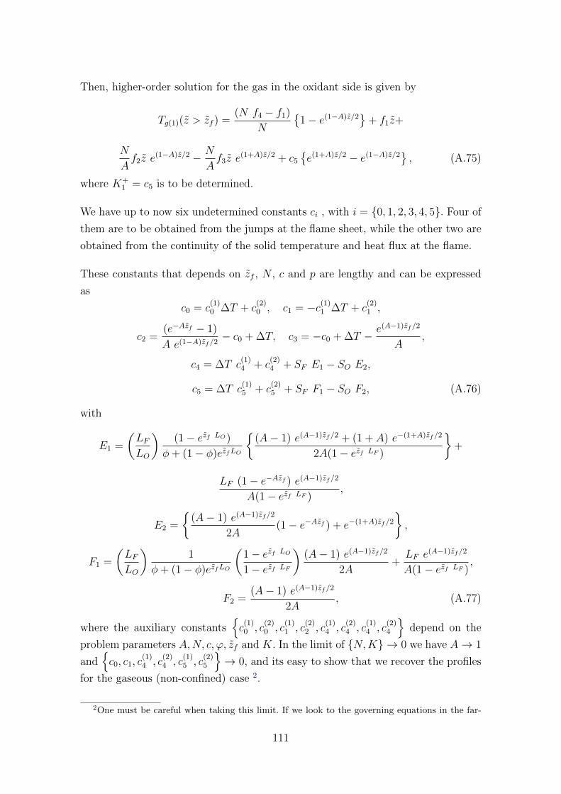
Then, higher-order solution for the gas in the oxidant side is given by
Tg(1)(z > zf ) =(N f4 − f1)
N
{1− e(1−A)z/2
}+ f1z+
N
Af2z e
(1−A)z/2 − N
Af3z e
(1+A)z/2 + c5
{e(1+A)z/2 − e(1−A)z/2
}, (A.75)
where K+1 = c5 is to be determined.
We have up to now six undetermined constants ci , with i = {0, 1, 2, 3, 4, 5}. Four of
them are to be obtained from the jumps at the flame sheet, while the other two are
obtained from the continuity of the solid temperature and heat flux at the flame.
These constants that depends on zf , N , c and p are lengthy and can be expressed
as
c0 = c(1)0 ∆T + c
(2)0 , c1 = −c(1)
1 ∆T + c(2)1 ,
c2 =(e−Azf − 1)
A e(1−A)zf/2− c0 + ∆T, c3 = −c0 + ∆T − e(A−1)zf/2
A,
c4 = ∆T c(1)4 + c
(2)4 + SF E1 − SO E2,
c5 = ∆T c(1)5 + c
(2)5 + SF F1 − SO F2, (A.76)
with
E1 =
(LFLO
)(1− ezf LO)
φ+ (1− φ)ezfLO
{(A− 1) e(A−1)zf/2 + (1 + A) e−(1+A)zf/2
2A(1− ezf LF )
}+
LF (1− e−Azf ) e(A−1)zf/2
A(1− ezf LF ),
E2 =
{(A− 1) e(A−1)zf/2
2A(1− e−Azf ) + e−(1+A)zf/2
},
F1 =
(LFLO
)1
φ+ (1− φ)ezfLO
(1− ezf LO
1− ezf LF
)(A− 1) e(A−1)zf/2
2A+LF e(A−1)zf/2
A(1− ezf LF ),
F2 =(A− 1) e(A−1)zf/2
2A, (A.77)
where the auxiliary constants{c
(1)0 , c
(2)0 , c
(1)1 , c
(2)2 , c
(1)4 , c
(2)4 , c
(1)4 , c
(2)4
}depend on the
problem parameters A,N, c, ϕ, zf and K. In the limit of {N,K} → 0 we have A→ 1
and{c0, c1, c
(1)4 , c
(2)4 , c
(1)5 , c
(2)5
}→ 0, and its easy to show that we recover the profiles
for the gaseous (non-confined) case 2.
2One must be careful when taking this limit. If we look to the governing equations in the far-
111
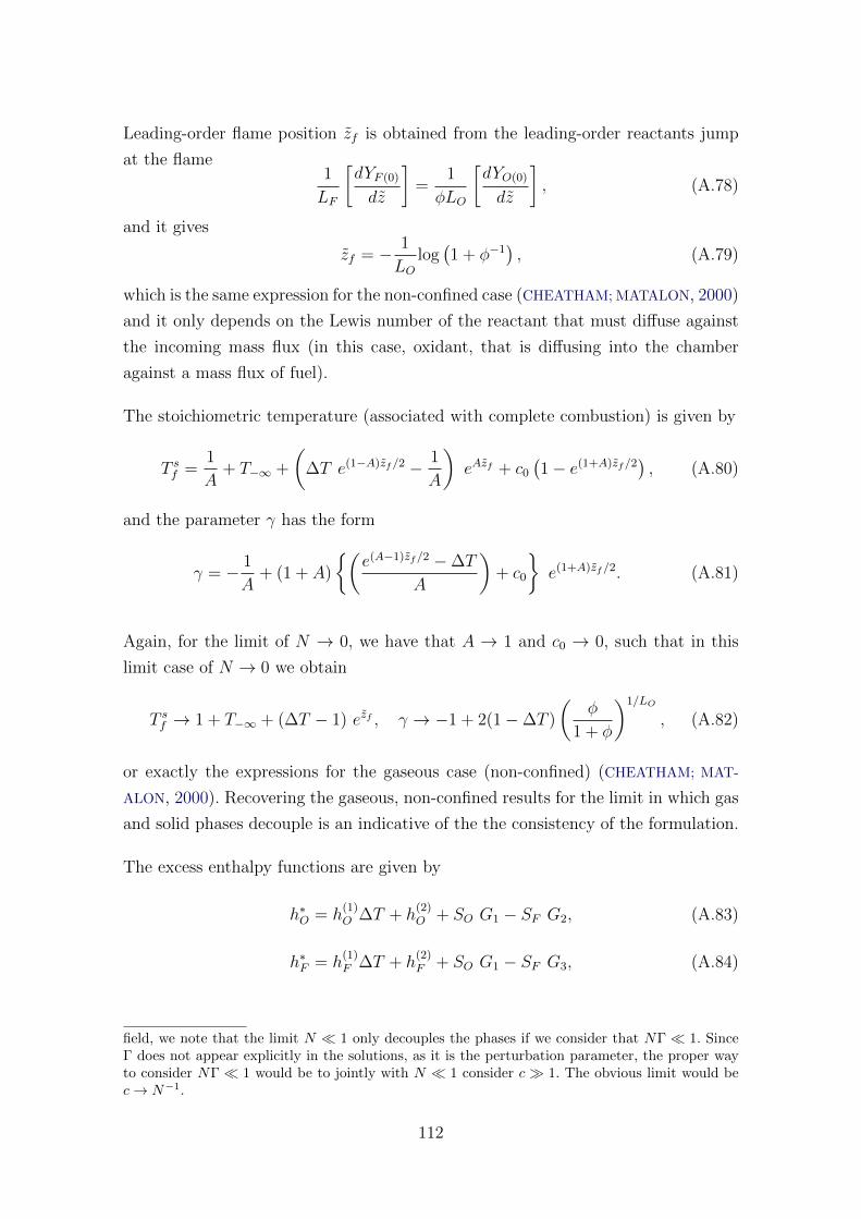
Leading-order flame position zf is obtained from the leading-order reactants jump
at the flame1
LF
[dYF (0)
dz
]=
1
φLO
[dYO(0)
dz
], (A.78)
and it gives
zf = − 1
LOlog(1 + φ−1
), (A.79)
which is the same expression for the non-confined case (CHEATHAM; MATALON, 2000)
and it only depends on the Lewis number of the reactant that must diffuse against
the incoming mass flux (in this case, oxidant, that is diffusing into the chamber
against a mass flux of fuel).
The stoichiometric temperature (associated with complete combustion) is given by
T sf =1
A+ T−∞ +
(∆T e(1−A)zf/2 − 1
A
)eAzf + c0
(1− e(1+A)zf/2
), (A.80)
and the parameter γ has the form
γ = − 1
A+ (1 + A)
{(e(A−1)zf/2 −∆T
A
)+ c0
}e(1+A)zf/2. (A.81)
Again, for the limit of N → 0, we have that A → 1 and c0 → 0, such that in this
limit case of N → 0 we obtain
T sf → 1 + T−∞ + (∆T − 1) ezf , γ → −1 + 2(1−∆T )
(φ
1 + φ
)1/LO
, (A.82)
or exactly the expressions for the gaseous case (non-confined) (CHEATHAM; MAT-
ALON, 2000). Recovering the gaseous, non-confined results for the limit in which gas
and solid phases decouple is an indicative of the the consistency of the formulation.
The excess enthalpy functions are given by
h∗O = h(1)O ∆T + h
(2)O + SO G1 − SF G2, (A.83)
h∗F = h(1)F ∆T + h
(2)F + SO G1 − SF G3, (A.84)
field, we note that the limit N � 1 only decouples the phases if we consider that NΓ � 1. SinceΓ does not appear explicitly in the solutions, as it is the perturbation parameter, the proper wayto consider NΓ � 1 would be to jointly with N � 1 consider c � 1. The obvious limit would bec→ N−1.
112
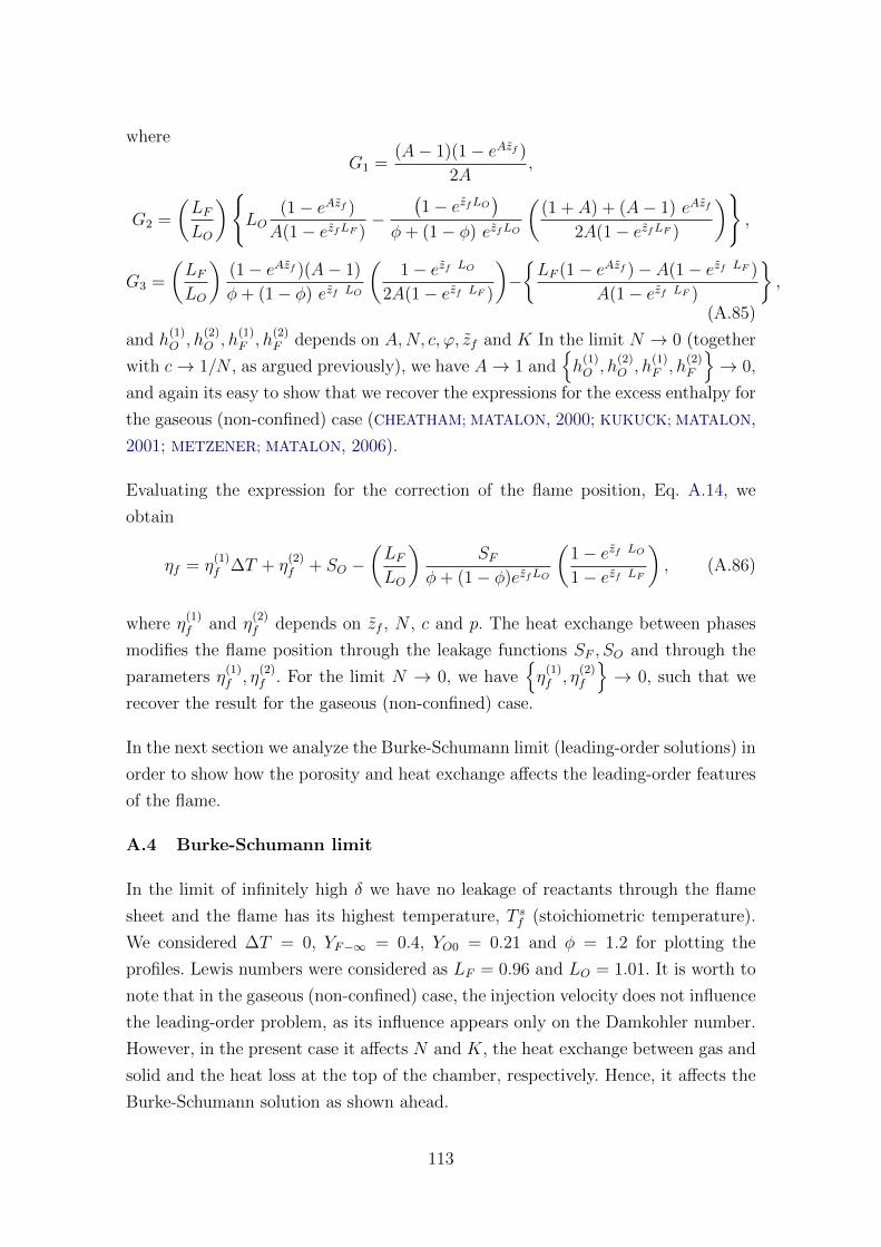
where
G1 =(A− 1)(1− eAzf )
2A,
G2 =
(LFLO
){LO
(1− eAzf )
A(1− ezfLF )−
(1− ezfLO
)φ+ (1− φ) ezfLO
((1 + A) + (A− 1) eAzf
2A(1− ezfLF )
)},
G3 =
(LFLO
)(1− eAzf )(A− 1)
φ+ (1− φ) ezf LO
(1− ezf LO
2A(1− ezf LF )
)−{LF (1− eAzf )− A(1− ezf LF )
A(1− ezf LF )
},
(A.85)
and h(1)O , h
(2)O , h
(1)F , h
(2)F depends on A,N, c, ϕ, zf and K In the limit N → 0 (together
with c→ 1/N , as argued previously), we have A→ 1 and{h
(1)O , h
(2)O , h
(1)F , h
(2)F
}→ 0,
and again its easy to show that we recover the expressions for the excess enthalpy for
the gaseous (non-confined) case (CHEATHAM; MATALON, 2000; KUKUCK; MATALON,
2001; METZENER; MATALON, 2006).
Evaluating the expression for the correction of the flame position, Eq. A.14, we
obtain
ηf = η(1)f ∆T + η
(2)f + SO −
(LFLO
)SF
φ+ (1− φ)ezfLO
(1− ezf LO
1− ezf LF
), (A.86)
where η(1)f and η
(2)f depends on zf , N , c and p. The heat exchange between phases
modifies the flame position through the leakage functions SF , SO and through the
parameters η(1)f , η
(2)f . For the limit N → 0, we have
{η
(1)f , η
(2)f
}→ 0, such that we
recover the result for the gaseous (non-confined) case.
In the next section we analyze the Burke-Schumann limit (leading-order solutions) in
order to show how the porosity and heat exchange affects the leading-order features
of the flame.
A.4 Burke-Schumann limit
In the limit of infinitely high δ we have no leakage of reactants through the flame
sheet and the flame has its highest temperature, T sf (stoichiometric temperature).
We considered ∆T = 0, YF−∞ = 0.4, YO0 = 0.21 and φ = 1.2 for plotting the
profiles. Lewis numbers were considered as LF = 0.96 and LO = 1.01. It is worth to
note that in the gaseous (non-confined) case, the injection velocity does not influence
the leading-order problem, as its influence appears only on the Damkohler number.
However, in the present case it affects N and K, the heat exchange between gas and
solid and the heat loss at the top of the chamber, respectively. Hence, it affects the
Burke-Schumann solution as shown ahead.
113
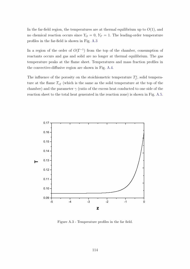
In the far-field region, the temperatures are at thermal equilibrium up to O(1), and
no chemical reaction occurs since YO = 0, YF = 1. The leading-order temperature
profiles in the far-field is shown in Fig. A.3
In a region of the order of O(Γ−1) from the top of the chamber, consumption of
reactants occurs and gas and solid are no longer at thermal equilibrium. The gas
temperature peaks at the flame sheet. Temperatures and mass fraction profiles in
the convective-diffusive region are shown in Fig. A.4.
The influence of the porosity on the stoichiometric temperature T sf , solid tempera-
ture at the flame Tsf (which is the same as the solid temperature at the top of the
chamber) and the parameter γ (ratio of the excess heat conducted to one side of the
reaction sheet to the total heat generated in the reaction zone) is shown in Fig. A.5.
-5 -4 -3 -2 -1 00.09
0.10
0.11
0.12
0.13
0.14
0.15
0.16
0.17
T
z
Figure A.3 - Temperature profiles in the far field.
114
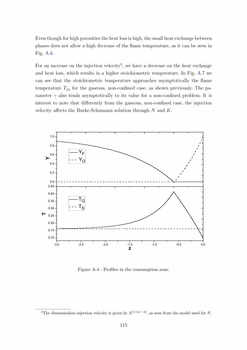
Even though for high porosities the heat loss is high, the small heat exchange between
phases does not allow a high decrease of the flame temperature, as it can be seen in
Fig. A.6.
For an increase on the injection velocity3, we have a decrease on the heat exchange
and heat loss, which results in a higher stoichiometric temperature. In Fig. A.7 we
can see that the stoichiometric temperature approaches asymptotically the flame
temperature Tfg for the gaseous, non-confined case, as shown previously. The pa-
rameter γ also tends asymptotically to its value for a non-confined problem. It is
interest to note that differently from the gaseous, non-confined case, the injection
velocity affects the Burke-Schumann solution through N and K.
0.0
0.2
0.4
0.6
0.8
1.0
-3.0 -2.5 -2.0 -1.5 -1.0 -0.5 0.0
0.10
0.15
0.20
0.25
0.30
0.35
0.40
0.45
Y
YF YO
T
z
TG TS
Figure A.4 - Profiles in the consumption zone.
3The dimensionless injection velocity is given by N1/(m′−2), as seen from the model used for N .
115
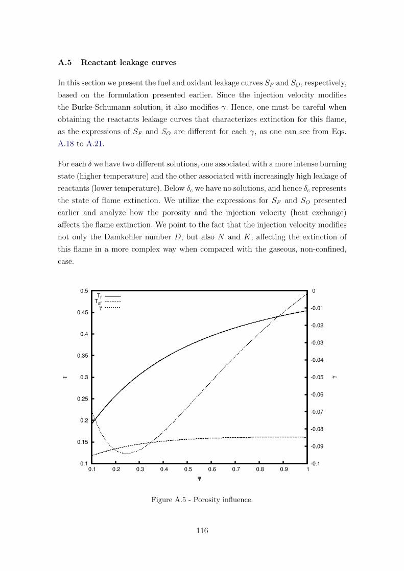
A.5 Reactant leakage curves
In this section we present the fuel and oxidant leakage curves SF and SO, respectively,
based on the formulation presented earlier. Since the injection velocity modifies
the Burke-Schumann solution, it also modifies γ. Hence, one must be careful when
obtaining the reactants leakage curves that characterizes extinction for this flame,
as the expressions of SF and SO are different for each γ, as one can see from Eqs.
A.18 to A.21.
For each δ we have two different solutions, one associated with a more intense burning
state (higher temperature) and the other associated with increasingly high leakage of
reactants (lower temperature). Below δc we have no solutions, and hence δc represents
the state of flame extinction. We utilize the expressions for SF and SO presented
earlier and analyze how the porosity and the injection velocity (heat exchange)
affects the flame extinction. We point to the fact that the injection velocity modifies
not only the Damkohler number D, but also N and K, affecting the extinction of
this flame in a more complex way when compared with the gaseous, non-confined,
case.
0.1
0.15
0.2
0.25
0.3
0.35
0.4
0.45
0.5
0.1 0.2 0.3 0.4 0.5 0.6 0.7 0.8 0.9 1-0.1
-0.09
-0.08
-0.07
-0.06
-0.05
-0.04
-0.03
-0.02
-0.01
0
T γ
ϕ
TfTsf
γ
Figure A.5 - Porosity influence.
116
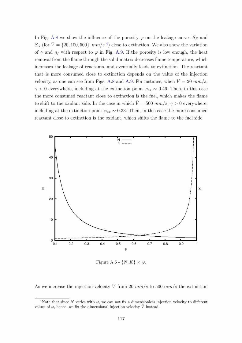
In Fig. A.8 we show the influence of the porosity ϕ on the leakage curves SF and
SO (for V = {20, 100, 500} mm/s 4) close to extinction. We also show the variation
of γ and ηf with respect to ϕ in Fig. A.9. If the porosity is low enough, the heat
removal from the flame through the solid matrix decreases flame temperature, which
increases the leakage of reactants, and eventually leads to extinction. The reactant
that is more consumed close to extinction depends on the value of the injection
velocity, as one can see from Figs. A.8 and A.9. For instance, when V = 20 mm/s,
γ < 0 everywhere, including at the extinction point ϕex ∼ 0.46. Then, in this case
the more consumed reactant close to extinction is the fuel, which makes the flame
to shift to the oxidant side. In the case in which V = 500 mm/s, γ > 0 everywhere,
including at the extinction point ϕex ∼ 0.33. Then, in this case the more consumed
reactant close to extinction is the oxidant, which shifts the flame to the fuel side.
0
10
20
30
40
50
0.1 0.2 0.3 0.4 0.5 0.6 0.7 0.8 0.9 1
N K
ϕ
NK
Figure A.6 - {N,K} × ϕ.
As we increase the injection velocity V from 20 mm/s to 500 mm/s the extinction
4Note that since N varies with ϕ, we can not fix a dimensionless injection velocity to differentvalues of ϕ, hence, we fix the dimensional injection velocity V instead.
117
porosity decreases and then increases. In a non-confined problem, an increase on the
injection velocity only decreases the Damkohler number. One could expect that a
similar behavior would occur for the confined case, but that is not the case. In the
present case, increasing the injection velocity first increase the Damkohler number up
to a maximum (as opposed to what happens in a non-confined problem), and further
increasing the injection velocity decrease the Damkohler number. Since for low V
we have a high value of the interphase heat exchange N , the intense heat transfer
between gas and solid decreases the stoichiometric flame temperature T sf , which
decreases exponentially the reactive Damkohler number D (from A.17, D ∼ e−Ta/Tsf ).
These features may be seen in Fig. A.10, where we show T sf and D as a function of
V for ϕ = 0.7.
The influence of the dimensionless injection velocity N1/(m′−2) on the reactants leak-
age is presented in Fig. A.11 with ϕ = 0.7, while in Fig. A.12 we present γ and ηf
variations with respect to the dimensionless injection velocity (as no porosity vari-
ation is considered here, the dimensionless velocity V ≡ N1/(m′−2) may be used). It
can be seen that the flame presents high leakage of reactants for both low and high
values of the injection velocity (Fig. A.13 show the low-velocity extinction point,
while Fig. A.14 show the high-velocity extinction point).
For the lower extinction point (low injection velocity and high heat exchange), more
heat is conducted from the flame sheet towards the fuel side, such that fuel is the
more consumed reactant, while for the higher extinction point (high injection velocity
and low heat exchange) the opposite holds, as seen in Figs. A.13 and A.14. For
N → 0, γ tends to its value on the gaseous, non-confined case, as shown in a
previous section. For high porosities, such that p = O(Γ−1), it can be shown that
the low extinction point (low injection velocity and high heat exchange) may be
eliminated. In other words, in this case, the flame supports higher amounts of heat
loss. However, when N = O(ε−1) � 1 the formulation breaks down, as the heat
exchange now occurs in the reaction region, and in this case the jumps at the flame
sheet must be modified, as the flame structure equations must consider the gas-solid
heat exchange.
It is interest to point that the existence of two extinction points was observed earlier
in the gaseous, non-confined case, when a finite chamber was considered (MATALON et
al., 1979; MATALON; LUDFORD, 1979), with a lower boundary through which gaseous
fuel was injected. In those works, when the fuel injection rate was low enough, the
flame was established close to the lower boundary, allowing high heat losses, such
118
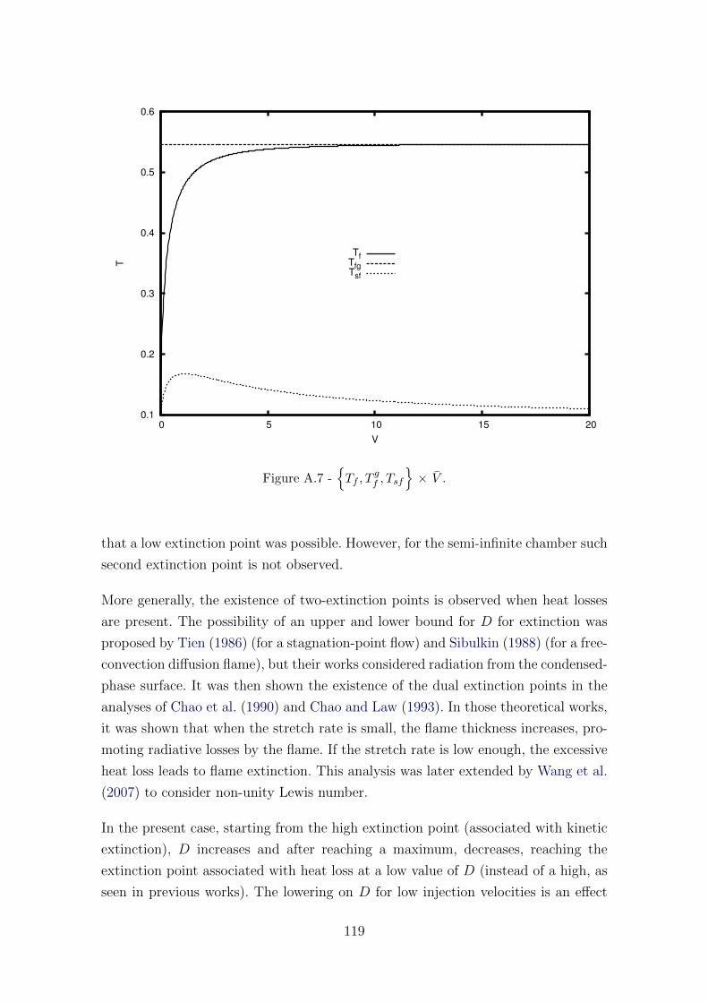
0.1
0.2
0.3
0.4
0.5
0.6
0 5 10 15 20
T
V
TfTfgTsf
Figure A.7 -{Tf , T
gf , Tsf
}× V .
that a low extinction point was possible. However, for the semi-infinite chamber such
second extinction point is not observed.
More generally, the existence of two-extinction points is observed when heat losses
are present. The possibility of an upper and lower bound for D for extinction was
proposed by Tien (1986) (for a stagnation-point flow) and Sibulkin (1988) (for a free-
convection diffusion flame), but their works considered radiation from the condensed-
phase surface. It was then shown the existence of the dual extinction points in the
analyses of Chao et al. (1990) and Chao and Law (1993). In those theoretical works,
it was shown that when the stretch rate is small, the flame thickness increases, pro-
moting radiative losses by the flame. If the stretch rate is low enough, the excessive
heat loss leads to flame extinction. This analysis was later extended by Wang et al.
(2007) to consider non-unity Lewis number.
In the present case, starting from the high extinction point (associated with kinetic
extinction), D increases and after reaching a maximum, decreases, reaching the
extinction point associated with heat loss at a low value of D (instead of a high, as
seen in previous works). The lowering on D for low injection velocities is an effect
119
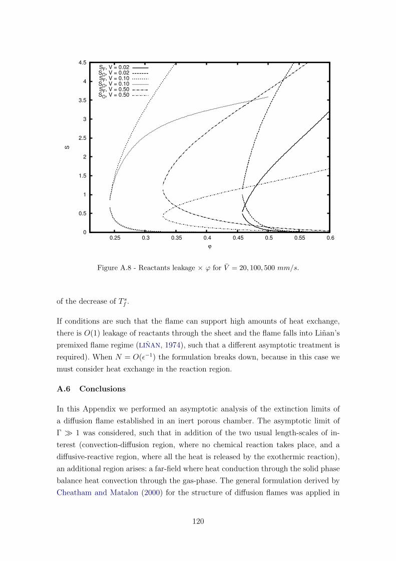
0
0.5
1
1.5
2
2.5
3
3.5
4
4.5
0.25 0.3 0.35 0.4 0.45 0.5 0.55 0.6
S
ϕ
SF, V = 0.02SO, V = 0.02SF, V = 0.10SO, V = 0.10SF, V = 0.50SO, V = 0.50
Figure A.8 - Reactants leakage × ϕ for V = 20, 100, 500 mm/s.
of the decrease of T sf .
If conditions are such that the flame can support high amounts of heat exchange,
there is O(1) leakage of reactants through the sheet and the flame falls into Linan’s
premixed flame regime (LINAN, 1974), such that a different asymptotic treatment is
required). When N = O(ε−1) the formulation breaks down, because in this case we
must consider heat exchange in the reaction region.
A.6 Conclusions
In this Appendix we performed an asymptotic analysis of the extinction limits of
a diffusion flame established in an inert porous chamber. The asymptotic limit of
Γ � 1 was considered, such that in addition of the two usual length-scales of in-
terest (convection-diffusion region, where no chemical reaction takes place, and a
diffusive-reactive region, where all the heat is released by the exothermic reaction),
an additional region arises: a far-field where heat conduction through the solid phase
balance heat convection through the gas-phase. The general formulation derived by
Cheatham and Matalon (2000) for the structure of diffusion flames was applied in
120
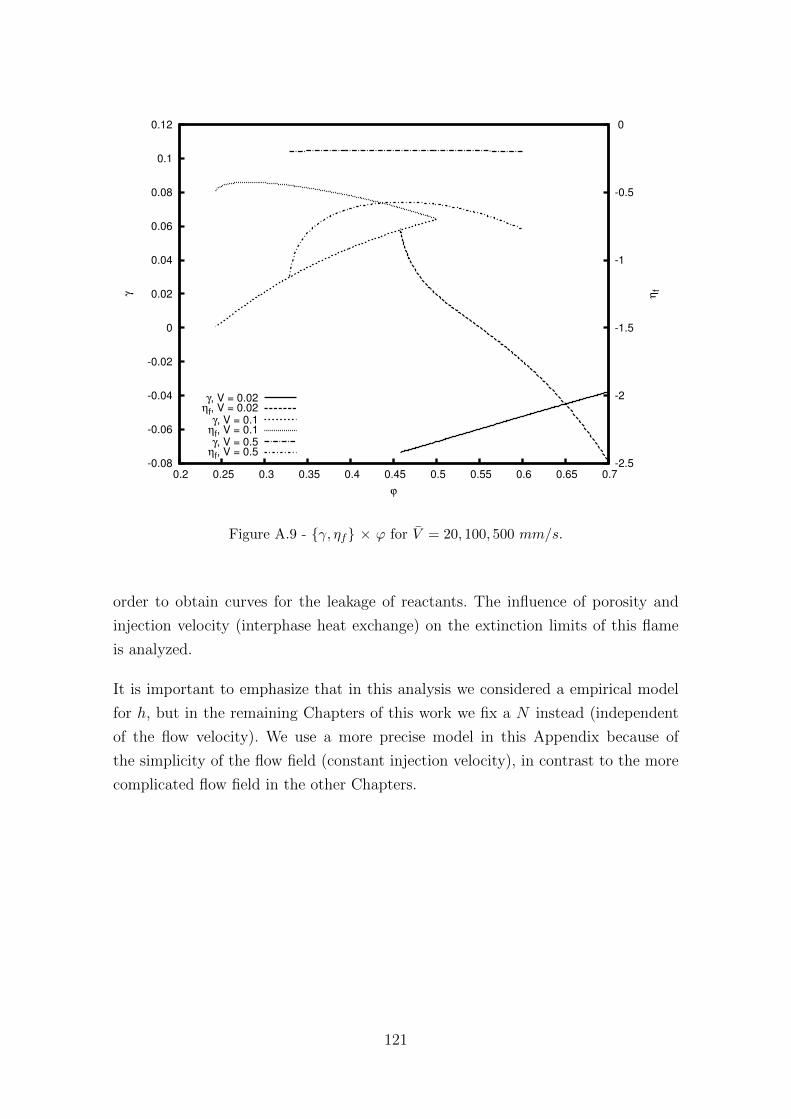
-0.08
-0.06
-0.04
-0.02
0
0.02
0.04
0.06
0.08
0.1
0.12
0.2 0.25 0.3 0.35 0.4 0.45 0.5 0.55 0.6 0.65 0.7-2.5
-2
-1.5
-1
-0.5
0γ ηf
ϕ
γ, V = 0.02ηf, V = 0.02
γ, V = 0.1ηf, V = 0.1γ, V = 0.5
ηf, V = 0.5
Figure A.9 - {γ, ηf} × ϕ for V = 20, 100, 500 mm/s.
order to obtain curves for the leakage of reactants. The influence of porosity and
injection velocity (interphase heat exchange) on the extinction limits of this flame
is analyzed.
It is important to emphasize that in this analysis we considered a empirical model
for h, but in the remaining Chapters of this work we fix a N instead (independent
of the flow velocity). We use a more precise model in this Appendix because of
the simplicity of the flow field (constant injection velocity), in contrast to the more
complicated flow field in the other Chapters.
121
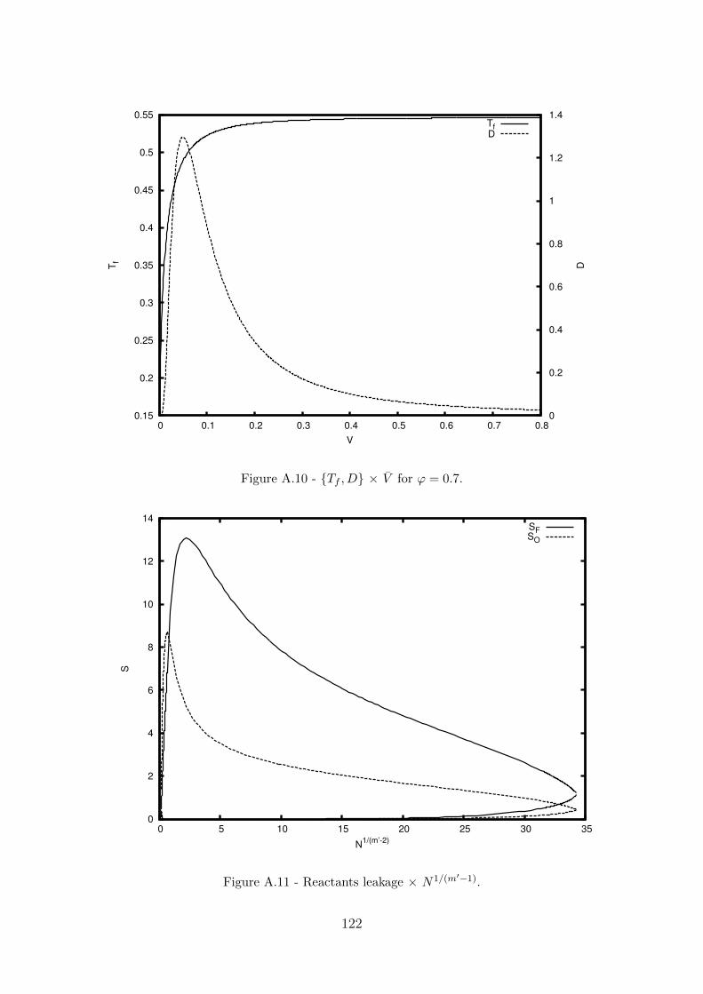
0.15
0.2
0.25
0.3
0.35
0.4
0.45
0.5
0.55
0 0.1 0.2 0.3 0.4 0.5 0.6 0.7 0.8 0
0.2
0.4
0.6
0.8
1
1.2
1.4T
f
D
V
TfD
Figure A.10 - {Tf , D} × V for ϕ = 0.7.
0
2
4
6
8
10
12
14
0 5 10 15 20 25 30 35
S
N1/(m’-2)
SFSO
Figure A.11 - Reactants leakage × N1/(m′−1).
122
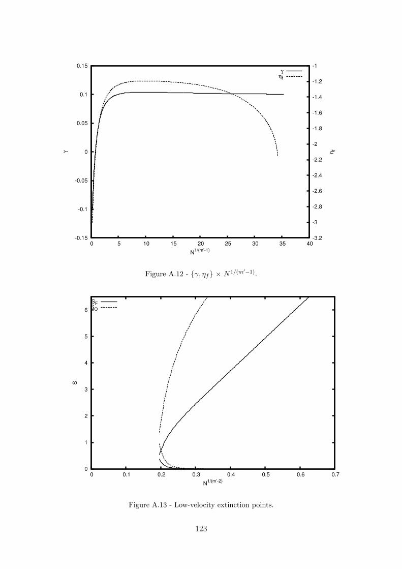
-0.15
-0.1
-0.05
0
0.05
0.1
0.15
0 5 10 15 20 25 30 35 40-3.2
-3
-2.8
-2.6
-2.4
-2.2
-2
-1.8
-1.6
-1.4
-1.2
-1γ ηf
N1/(m’-1)
γηf
Figure A.12 - {γ, ηf} × N1/(m′−1).
0
1
2
3
4
5
6
0 0.1 0.2 0.3 0.4 0.5 0.6 0.7
S
N1/(m’-2)
SFSO
Figure A.13 - Low-velocity extinction points.
123
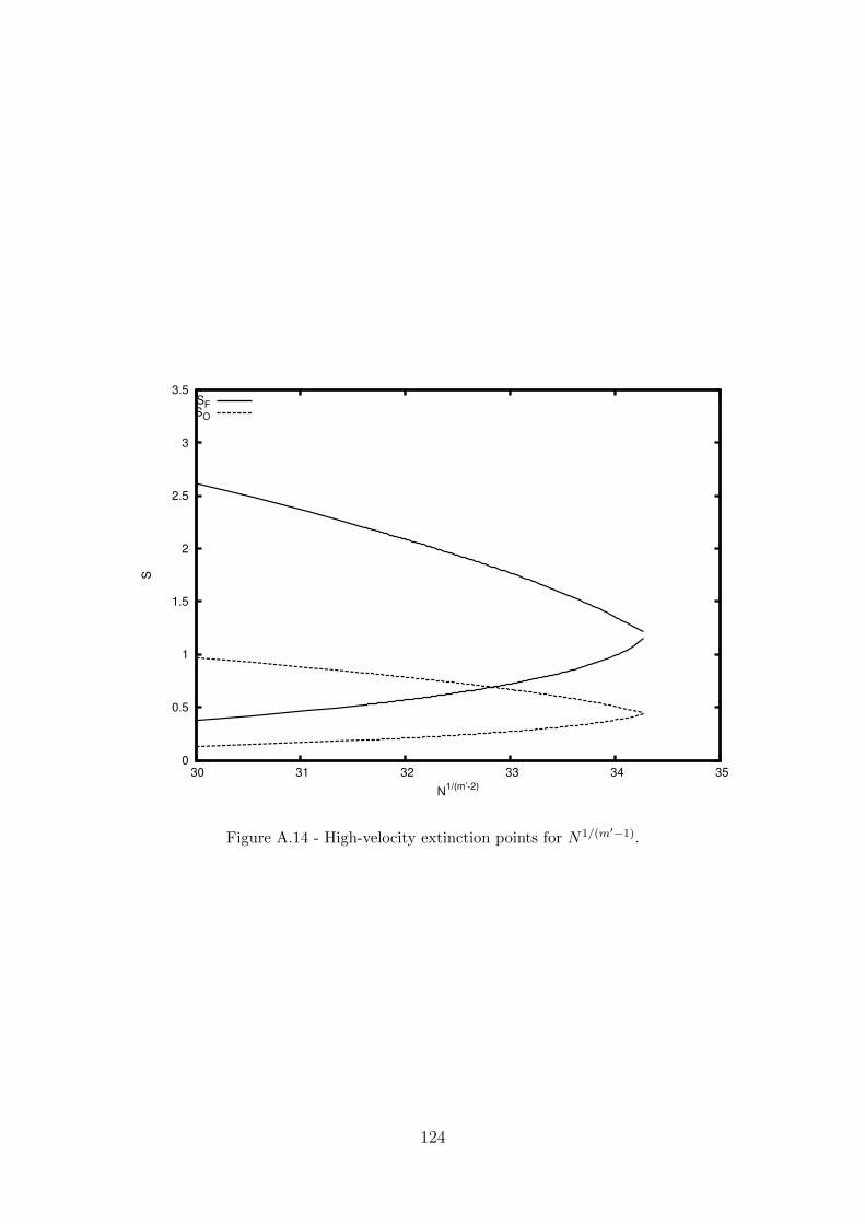
0
0.5
1
1.5
2
2.5
3
3.5
30 31 32 33 34 35
S
N1/(m’-2)
SFSO
Figure A.14 - High-velocity extinction points for N1/(m′−1).
124
PUBLICACOES TECNICO-CIENTIFICAS EDITADAS PELO INPE
Teses e Dissertacoes (TDI) Manuais Tecnicos (MAN)
Teses e Dissertacoes apresentadas nosCursos de Pos-Graduacao do INPE.
Sao publicacoes de carater tecnico queincluem normas, procedimentos, in-strucoes e orientacoes.
Notas Tecnico-Cientıficas (NTC) Relatorios de Pesquisa (RPQ)
Incluem resultados preliminares depesquisa, descricao de equipamentos,descricao e ou documentacao de progra-mas de computador, descricao de sis-temas e experimentos, apresentacao detestes, dados, atlas, e documentacao deprojetos de engenharia.
Reportam resultados ou progressos depesquisas tanto de natureza tecnicaquanto cientıfica, cujo nıvel seja com-patıvel com o de uma publicacao emperiodico nacional ou internacional.
Propostas e Relatorios de Projetos(PRP)
Publicacoes Didaticas (PUD)
Sao propostas de projetos tecnico-cientıficos e relatorios de acompan-hamento de projetos, atividades e con-venios.
Incluem apostilas, notas de aula e man-uais didaticos.
Publicacoes Seriadas Programas de Computador (PDC)
Sao os seriados tecnico-cientıficos: bo-letins, periodicos, anuarios e anais deeventos (simposios e congressos). Con-stam destas publicacoes o InternacionalStandard Serial Number (ISSN), que eum codigo unico e definitivo para iden-tificacao de tıtulos de seriados.
Sao a sequencia de instrucoes ou codi-gos, expressos em uma linguagem deprogramacao compilada ou interpre-tada, a ser executada por um computa-dor para alcancar um determinado obje-tivo. Aceitam-se tanto programas fontequanto os executaveis.
Pre-publicacoes (PRE)
Todos os artigos publicados em periodi-cos, anais e como capıtulos de livros.