THEORY OF MARTENSITIC MICROSTRUCTURE

AND THE SHAPE-MEMORY EFFECT

KAUSHIK BHATTACHARYADivision of Engineering & Applied Science104-44 California Institute of Technology

Pasadena, CA 91125 USAEmail: bhatta@cco.caltech.edu

Keywords: Shape-memory eect, Martensitic phase transformation, Crystallography, Microstruc-ture, Twinning, Habit Plane, Self-accommodation, Recoverable strain, Polycrystal.

Abstract

This chapter describes a theory of martensitic microstructure. The theory explains why marten-sites form microstructure and describes how this microstructure depends, often delicately, on thecrystalline symmetry and the lattice parameters. The shape-memory eect is analyzed with thistheory and it is shown that only very special materials those that satisfy signicant restrictonson their symmery and lattice parameters can display this eect.

1 Introduction

Martensitic phase transformation is observed in various metals, alloys, ceramics and even biologicalsystems. In this solid to solid phase transformation, the lattice or molecular structure changesabruptly at some temperature. The change is sudden, so a graph of lattice parameter vs. tempera-ture shows a marked discontinuity. Further, there is no diusion or rearrangement of atoms duringthis transformation. Therefore, this transformation is often said to be a displacive rst-order phasetransformation.

Martensitic phase transformations have many important technological implications. The oldest,and by far the most signicant, is its role in strengthening steel. A recent volume edited by Olsonand Owen [1] provides an interesting overview of the history, signicance and scientic interestin this phase transformation. The shape-memory eect is one technological manifestation of thistransformation that has received much attention in the recent years. A recent proceeding of theInternational Conference on Martensitic Transformations [2] gives a glimpse of the interest in theshape-memory eect.

The most characteristic observable feature of a martensitic transformation is the microstruc-ture it produces. In a typical transformation, the high-temperature austenite phase has greatercrystallographic symmetry than the low-temperature martensite phase. This gives rise to multiplesymmetry-related variants of martensite. These variants of martensite form complex patterns at alength-scale much smaller than the size of the specimen. The actual length-scale can range froma few nanometers to tenths of millimeters and it depends on a variety of factors including thematerial, specimen size, grain size and history. The microstructure endows the material with itsproperties.

The goal of this chapter is to present a theory that explains the formation and describes variousimportant aspects of this microstructure. This is a continuum theory, built on the framework of

2

thermoelasticity. It is phenomenological to the extent that it starts with the observation of thetransformation. The change in symmetry and the transformation strain are its only inputs. Itshows that the microstructure arises as a consequence of energy minimization. More importantly,it predicts various aspects of the microstructure, and consequently the macroscopic properties, withno further assumptions.

A particular point of interest is the shape-memory eect. A whole host of materials undergomartensitic transformation; however, negligibly few display the shape-memory eect. This chapterexplores the crystallographic reasons that make shape-memory alloys special amongst martensites.We will see that the shape-memory eect requires special changes in symmetry and also verydelicate relations between the lattice parameters. This issue has important technological relevance.Despite the vast potential, the incorporation of shape-memory alloys into applications has beenslow. Though a sizable number of alloys are known, applications have essentially been limitedto Nickel-Titanium (at compositions close to equiatomic) for a variety of reasons. The high costof NiTi as well as the narrow temperature range in which it can be used have placed additionallimitations. Therefore, it is important to improve and stabilize the shape-memory eect in knownmaterials and develop new materials.

This chapter draws heavily on the recent advances in the mathematical modeling and analysisof martensites. These unfortunately have often been inaccessible to some. This chapter is anattempt to overcome this. Therefore, it is not a comprehensive or up-to-date review. Instead, it isan attempt to explain the main ideas and give a avor of the results.

I have assumed only a college-level knowledge of mathematics. I believe that the essentialconcepts can be explained at this level and I have tried to do so. Consequently, I have taken someliberties with the jargon and some technical details. Also, some of the calculations are longer thatthey need to be. However, I have consciously decided not to hide the mathematics. I hope that Ihave been able to convey the benets of a mathematical approach through this.

This is a very good point to refer to some related literature outside of this book and the originalpapers. Saburi and Nenno [3], Tadaki, Otsuka and Shimizu [4], Miyazaki and Otsuka [5] andWayman [6] are excellent reviews of the shape-memory eect. The book by Wayman [7] is a classicsummary of the crystallographic theory. The theory presented in this chapter builds on the ideaspresented in these and attempts to make them quantitative and consequently predictive. The bookby Ball and James [8] is a detailed exposition of the theory presented here and its results.

The rest of the introduction is a road map through this chapter. I have tried to begin everysection with the simplest and the most essential elements; so a reader stuck at one point canmove over to the next subsection during the rst reading. We begin with a brief introduction tovector algebra and the continuum description of deformation in Sec. 2. Sec. 3 provides a generalintroduction to a continuum theory of crystalline solids.

The martensitic phase transformation is introduced in Sec. 4. It discusses the transformationor Bain matrix, the variants, the energy wells and other important concepts. I have tried to keepthis section self-contained to the extent that a reader familiar with martensitic transformations candirectly proceed to Sec. 4 and refer back to Secs. 2 and 3 whenever necessary.

Sec. 5 discusses twinning. It shows that all the twinning modes and their crystallographic detailscan be obtained as a consequence of symmetry and the transformation matrix. This gives a glimpseof how much one can predict from the easily measurable quantities symmetry and transformationmatrix.

Sec. 6 shows that energy minimization with many variants naturally results in microstructure.This section also introduces a very nice way of describing a microstructure through a sequence ofdeformations with ner and ner details.

Some important examples of microstructure are discussed in Sec. 7. These examples show that

3

the theory can accurately predict various crystallographic details of the microstructure. The rst isthe austenite-martensite interface. We show that we can derive the well-known crystallographic orphenomenological theory of martensite. This theory proposed independently by Wechsler, Lieber-man and Read[9] as well as Bowles and Mackenzie[10], arguably far ahead of its time, is one ofthe most signicant results in this subject. The current presentation following Ball and James [11]derives it as a consequence of energy minimization and does not require the a priori knowledge ofthe twinning modes etc. Further, putting these ideas in a systematic framework allows us to extendthem to other situations. We do so with the wedge-like microstructure. This is a very interestingexample. We will see that only very special materials, those whose lattice parameters satisfy somerather strict restrictions, can form this microstructure. This shows us that the microstructure andconsequently the macroscopic properties can depend very delicately on the lattice parameters.

Following these methods one can construct a whole host of microstructures. However, we cannot address the following question can a material form a microstructure which satises some givenboundary condition? An example of such a question is, can a material form a self-accommodatingmicrostructure? If we are lucky or suciently innovative, we can successfully construct one. On theother hand, if we are unable to do so, we can never decide whether such a microstructure is simplynot possible or whether we should try harder. Further, constructing a complicated microstructurerequires very cumbersome calculations. All this points to the need for more general tools to addresssuch questions. We discuss the average compatibility conditions or the minors relations in Sec. 8.These are simple algebraic restrictions that all microstructures must satisfy. Therefore, it providesa very easy check for deciding whether some microstructure is possible.

We discuss the shape-memory eect in single crystals in Sec. 9. We begin with self-accommodation.The results show that a material with a cubic austenite that undergoes a volume-preserving trans-formation can always form a self-accommodating microstructure. A material whose symmetry isnot cubic, on the other hand, has to satisfy some impossibly strict restriction on its lattice parame-ters in order to be self-accommodating. This explains why all the shape-memory alloys have cubicaustenite and undergo volume-preserving transformation. We then discuss recoverable strains un-der both load and displacement control. We see that relatively little is known under displacementcontrol. Sec. 10 brie y discusses polycrystals. Sec. 11 gathers the important ideas and resultsincluding the implications for the shape-memory eect.

2 Review of Linear Algebra and Continuum Mechanics

In this section, we quickly review some basic aspects of linear algebra and some basic kinematicconcepts of continuum mechanics. A reader who nds this review insucient is referred to somestandard books on continuum mechanics like [12, 13, 14]. We conne our attention to three dimen-sions.

2.1 Vectors and Matrices

We denote vectors using bold lower-case Roman letters and their components with respect toa \rectangular Cartesian basis" using plain lower-case Roman letters with one subscript. Forexample,

a = fa1; a2; a3g: (2.1)

We denote the dot product or inner product between two vectors a and b as a b. Recall that

a b = a1b1 + a2b2 + a3b3: (2.2)

4

Rather than writing such long formulas, we use the summation convention where repeated indicesare summed. Using this convention,

a b = aibi: (2.3)

We denote 3 3 matrices using bold upper-case Roman letters and their components usingplain upper-case Roman letters with two subscripts. For example,

A =

0B@ A11 A12 A13

A21 A22 A23

A31 A32 A33

1CA : (2.4)

From now on, whenever we say matrix, we mean a 33 matrix. In any xed rectangular Cartesianbasis, a matrix denes a linear transformation or a tensor. Therefore, it maps one vector intoanother. For example, consider the equation

b = Aa (2.5)

which can be written in standard matrix notation as0B@ b1b2b3

1CA =

0B@ A11 A12 A13

A21 A22 A23

A31 A32 A33

1CA0B@ a1a2a3

1CA : (2.6)

This equation says that the matrix A takes the vector a to vector b or the the matrix A acts onthe vector a to give us vector b. We can use the summation convention to rewrite Eq. (2.6) as

ai = Aijbj for i = 1; 2; 3: (2.7)

According to the summation convention, the repeated index j is summed. Thus, we have threeequations

b1 = A11a1 +A12a2 + A13a3b2 = A21a1 +A22a2 + A23a3b3 = A31a1 +A32a2 + A33a3

(2.8)

where the rst line corresponds to i = 1, the second to i = 2 and the third to i = 3. Whenever itis clear from the context, we will omit the phrase \for i = 1; 2; 3".

We now dene a matrix which will play a crucial role in the discussion of coherence. Givenany two vectors a and b, the matrix a b (pronounced a tensor b or a dyadic b) has components(a b)ij = aibj for i; j = 1; 2; 3, or

a b =

0B@ a1b1 a1b2 a1b3a2b1 a2b2 a2b3a3b1 a3b2 a3b3

1CA : (2.9)

To understand this matrix, let it act on any vector v. It is easy to verify that

(a b)v = (b v)a (2.10)

Therefore, it takes any vector v to a vector which is parallel to a and whose magnitude is propor-tional to (b v). In particular, if v is perpendicular to b, the result is the zero vector.

5

F1 denotes the inverse of the matrix F, FT denotes the transpose and FT the inverse of thetranspose or the transpose of the inverse. detF denotes the determinant of F while cof F denotesthe cofactor matrix of F. All thes have their usual meaning. In particular, if detF 6= 0, then

cof F = (detF)FT : (2.11)

We say that Q is a rotation if QQT = QTQ = I and detQ = 1 where I is the identity matrix.We say that Q is a re ection or inversion if QQT = QTQ = I and detQ = 1.

We say that U is symmetric if U = UT . A symmetric matrix has three real eigenvaluesf1; 2; 3g; further we can choose eigenvectors fe1; e2; e3g corresponding to the eigenvalues abovesuch that they are mutually perpendicular unit vectors. We say that U is positive-denite ifa Ua > 0 (or aiUijaj > 0 in components) for all vectors a 6= 0. All eigenvalues of a symmetricpositive-denite matrix are positive.

We are now in a position to state a very important result. We will use this result in the nextsection to decompose any deformation into a pure stretch and a rotation.

Theorem 2.1. Polar decomposition theorem. Consider any matrix F with detF > 0. There existsan unique rotation Q and an unique positive-denite symmetric matrix U such that

F = QU: (2.12)

In fact, U =pFTF and Q = FU1. We can calculate these using the following procedure.

Procedure 2.2. Procedure to calculate the polar decomposition.

1. Calculate the matrix C = FTF. It is possible to verify that C is symmetric and positive-denite.

2. Calculate the eigenvalues f 1; 2; 3g of C and the corresponding mutually perpendiculareigenvectors fu1; u2; u3g. Automatically, i > 0 because C is positive-denite.

3. Calculate i =p i; i = 1; 2; 3 taking care to choose the positive root so that i > 0.

4. U is the matrix with eigenvalues f1; 2; 3g and corresponding eigenvectors fu1; u2; u3g, or

U = 1u1 u1 + 2u2 u2 + 3u3 u3: (2.13)

5. Finally calculateQ = FU1: (2.14)

Notice above that we have introduced the idea of the square-root of a positive-denite symmetricmatrix. U =

pC is the unique positive-denite symmetric matrix with the property that U2 = C.

U has the same eigenvectors as C, but the eigenvalues of U are the square-roots of those of C.

2.2 Continuum Kinematics

2.2.1 Deformation

Consider a body occupying a region in three-dimensional space IR3 as shown in Fig. 2.1. Let uschoose this to be the reference conguration; in other words, we use this conguration to describe

6

q

xn

dx

dV

rdA

dv

y(x)

dyda

m

y

Ω y(Ω)

p

y(q)

y(p)y(r)

Figure 2.1: The deformation y takes the reference conguration on the left to the deformed con-guration on the right.

2

1

0 1 2 3

x (y )2 2

x (y )1 1

Figure 2.2: Example of a homogeneous deformation. The reference conguration on the left deformsto the deformed conguration on the right under the deformation described in Eq. (2.15).

7

x (y )2 2

x (y )1 1

1

0 1 2 3

Figure 2.3: Example of an inhomogeneous deformation. The reference conguration on the leftdeforms to the deformed conguration on the right under the deformation described in Eq. (2.16).Notice that under sucient magnication, an inhomogeneous deformation can be approximatedlocally by a homogeneous deformation.

the body. Let x = fx1; x2; x3g be a typical point in . We call the particle occupying the position x,the particle x. Now, deform the body. The deformation may be described as a function y : ! IR3

where y(x) = fy1(x); y2(x); y3(x)g denotes position of the particle x in the deformed conguration.

Fig. 2.2 shows a simple deformation

y1 = (1p2)x1

p2x2 + 3; y2 = (

1p2)x1 +

p2x2; y3 = x3: (2.15)

We choose the reference conguration to be an unit cube as shown on the left. Notice that thisdeformation is planar because y3 = x3 and we can draw it on a sheet of paper. To completelyunderstand the deformation, we have placed a grid in the reference conguration and followed itsdeformation. This deformation translates the body to the right, stretches it in the \x2" directionand then rotates it counter-clockwise by 45o. Notice that in this deformation, each part of thebody has undergone the same distortion; such deformations are known as uniform or homogeneous

deformations.

Fig. 2.3 shows another planar deformation,

y1 = x1 + 0:1 sin(2x2) + 2; y2 = x2 + 0:1x1; y3 = x3: (2.16)

of the unit cube. Once again, we follow the deformation of a grid. Notice that in this case, thedeformation is not uniform; so we call this an inhomogeneous deformation.

2.2.2 Deformation Gradient

Given any deformation y, the deformation gradient ry is the matrix of partial derivatives; i.e., itis the matrix with components

(ry)ij = @yi@xj

i; j = 1; 2; 3: (2.17)

For convenience, we often use F to denote the deformation gradient, i.e., we set F(x) = ry(x).

8

For example, in the deformations Eq. (2.15) shown in Fig. 2.2 and Eq. (2.16) shown in Fig. 2.3,the deformation gradients are easily calculated to be

F(x) =

0BBBBBB@

1p2

p2 0

1p2

p2 0

0 0 1

1CCCCCCA

(2.18)

and

F(x) =

0B@ 1 0:2 cos(2x2) 0

0:1 1 00 0 1

1CA (2.19)

respectively. Notice that the deformation gradient is constant in the homogeneous deformation,but it is not constant in the inhomogeneous deformation. In fact, any homogeneous deformationcan be written as

y = Fx+ c (2.20)

for some constant matrix F and constant vector c. For example, we obtain the deformation Eq.(2.15) if we take F as in Eq. (2.18) and c = f3; 0; 0g.

The deformation gradient plays a very important role in describing the \local" or \innitesimal"nature of the deformation. Suppose we consider a very small region of the body and magnify it. Forexample, let us take a little square and magnify it as shown in Fig. 2.3. Let us once again put a gridon it and then look at this square after deformation: it looks like a parallelopiped. However, noticethat at this magnication, the deformation looks almost homogeneous. Indeed, F(x) describes thisalmost homogeneous deformation close to the material point x.

The deformation gradient also gives us information on the deformation of innitesimal elementsof length, area and volume. We will now show that innitesimal line elements near a material pointx deform according to F(x), surface elements deform according to cof F(x) while volume elementsdeform according to detF(x). Thus, the deformation gradient F(x) provides a full characterizationof the deformation of innitesimal elements of length, area and volume near a particle x.

Consider an innitesimal line element dx at the point p in the reference conguration as shownin Fig. 2.1. dx = fdx1; dx2; dx3g is a vector with innitesimally small length in some direction.After deformation, this goes to the element dy. It is possible to show1 that

dy = F(p)dx: (2.21)

For example, consider the deformation Eq. (2.15) shown in Fig. 2.2. Since this is a homogeneousdeformation, the statement above is true not only for an innitesimal line element, but also for anite line. Consider the vector v = f1; 1; 0g in the reference conguration (this is the vector whichgoes from the lower left to the upper right corner). According to Eq. (2.21), it goes to the vector

Fv =

0BBBBBB@

1p2

p2 0

1p2

p2 0

0 0 1

1CCCCCCA

0BBBBB@

1

1

0

1CCCCCA =

1p2

0BBBBB@

1

3

0

1CCCCCA (2.22)

1Write down the Taylor expansion of y(x) near the point p and use the denition of the deformation gradient.

9

As expected, this is the vector that goes from the bottom to top corner in the deformed congura-tion.

Therefore, we can use the deformation gradient to calculate the strain in any direction. We willnow show that the

strain in the direction e =

qe (FTFe)

1: (2.23)

Consider an innitesimal line element dx in the direction e in the reference conguration. Afterdeformation, it goes to dy = Fdx according to Eq. (2.21). Therefore,

strain =nal length initial length

initial length

=jdyj jdxj

jdxj =jdyjjdxj 1 =

pdy dyjdxj 1

=

p(Fdx) (Fdx)

jdxj 1 =

sFdx

jdxjFdx

jdxj !

1 (2.24)

=

q(Fe) (Fe)

1 =

qe (FTFe)

1:

Let us go back to our example Eq. (2.15) shown in Fig. 2.2 and consider the direction v =f1; 1; 0g=p2 in the reference conguration which points from the lower left to the upper rightcorner. It is easy to use the formula above to calculate the strain to be

p5=2 1. This is easily

veried from the gure: notice that the length of the diagonal in the reference conguration isp2

while that in the deformed conguration isp5 so that the strain is (

p5p2)=p2 = p

5=2 1.Now consider a dierential material volume dV at the material point q in the reference con-

guration in Fig. 2.1. After deformation, this goes to the dierential volume dv. It is possible toshow that

dv = (detF(q))dV: (2.25)

Thus, the determinant of the deformation gradient describes the local change in volume. Once againconsider the deformation Eq. (2.15) shown in Fig. 2.2. As before, we may look at nite rather thaninnitesimal volumes because this deformation is homogeneous. According to Eq. (2.25) and Eq.(2.18), the ratio of the deformed to reference volumes is equal to detF = 2.

We are interested in only those deformations where a nite volume is not compressed to a pointor where a point is not expanded to a nite volume. Further, we we are interested in only thosedeformations where the body does not penetrate itself. Therefore, we will assume that detF > 0at all points within the body.

Finally consider the dierential material area dA with unit normal n in the reference congu-ration. After deformation, this goes to the dierential area da with unit normal m (see Fig. 2.1).It turns out that

m =FT njFT nj while da = dAj(cof F)nj: (2.26)

In fact, there is an easier way of writing these relations. Let us introduce the idea of an \area vector"for any planar surface. The area vector a of any planar surface is the vector whose magnitude jajis equal to the surface area and whose direction a=jaj is the normal. Therefore, (dAn) is the areavector of the innitesimal surface element in the reference conguration while (dam) is the areavector in the deformed conguration. We can summarize the relations in Eq. (2.26) above as

dam = (cof F)(dAn): (2.27)

10

Thus, the cofactor of the deformation gradient describes the local change in area. Let us nowexamine this for the deformation Eq. (2.15) shown in Fig. 2.2. Consider the plane with normaln = 1p

2f1; 1; 0g which goes through the bottom-right and the top-left corners of the reference

conguration. After deformation, this plane goes to the plane which passes through the left andright corners in the deformed conguration. Let us see what Eq. (2.27) gives us.

(cof F)n =

0BBBBBB@

p2 1p

20

p2 1p

20

0 0 2

1CCCCCCA

0BBBBBB@

1p2

1p2

0

1CCCCCCA=

1

2

0BBBBB@

1

3

0

1CCCCCA ; (2.28)

so that the ratio of deformed to reference area is j(cof F)nj =p5p2as expected. Further, the normal

to the deformed plane is m = 1p10f1; 3; 0g which is easily veried in the gure.

Let us conclude with one nal observation. Notice that line segments and normals to planesdeform quite dierently. In the example above, we picked v and n to be parallel, but Fv and mare not.

2.2.3 Rotation and Stretch

We now show that we can decompose any deformation locally into a stretch or pure distortionfollowed by a pure rotation. We will use this decomposition later in our discussion of frame-indierence.

It is very easy to see this decomposition for the the homogeneous deformation Eq. (2.15) shownin Fig. 2.2. Notice that we can decompose the deformation gradient F given in Eq. (2.18) as follows:

0BBBBBB@

1p2

p2 0

1p2

p2 0

0 0 1

1CCCCCCA=

0BBBBBB@

1p2

1p2

0

1p2

1p2

0

0 0 1

1CCCCCCA

0BBBBB@

1 0 0

0 2 0

0 0 1

1CCCCCA : (2.29)

It is clear that the rst matrix on the right is a rotation (of 45o about the 3-axis) while the secondis positive-denite and symmetric . We will call the rst Q and the second U. U stretches thereference conguration in the x2 direction and Q rotates it by 45o in the counter-clockwise manner.Therefore, this deformation is a stretch or distortion by U followed by a rotation by Q.

In general, we use the polar decomposition theorem (Theorem 2.1) to decompose the de-formation gradient F(x) into a rotation Q(x) and a positive-denite symmetric matrix U(x):F(x) = Q(x)U(x). Consider an innitesimal sphere near the material point x. U(x) stretches thissphere by the amounts equal to its eigenvalues i in the direction of its eigenvectors ui to obtain anellipsoid; Q(x) then rotates this to become the nal deformed ellipsoid. U is called the stretch andQ is called the rotation associated with the deformation gradient. U(x) describes the \distortion"in a small region near x while Q(x) describes the \orientation".

2.2.4 Kinematic Compatibility

We now turn to another crucial aspect of deformation. Consider the deformation shown in Fig.2.4. The bottom part of the body has been sheared one way while the top part has been sheared in

11

m

y = Fx + c

y = Gx + d

Ω1

2Ω

n

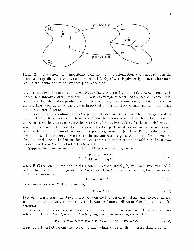
Figure 2.4: The kinematic compatibility condition. If the deformation is continuous, then thedeformation gradients on the two sides must satisfy Eq. (2.31). Equivalently, coherent interfacesrequire the satisfaction of an invariant plane condition.

another; yet the body remains unbroken. Notice that a straight line in the reference conguration iskinked, but unbroken after deformation. This is an example of a deformation which is continuous,but where the deformation gradient is not. In particular, the deformation gradient jumps acrossthe interface. Such deformations play an important role in the study of martensites; in fact, theydescribe coherent interfaces.

If a deformation is continuous, can the jump in the deformation gradient be arbitrary? Lookingat the Fig. 2.4, it is easy to convince ourself that the answer is no. If the body has to remainunbroken, then the plane separating the two sides of the body should suer the same deformationwhen viewed from either side. In other words, the two parts must contain an \invariant plane".Alternately, recall that the deformation of the plane is governed by (cof F)n. Thus, if a deformationis continuous, then this quantity must remain unchanged as we go across the interface. Therefore,the jump or change in the deformation gradient across the surface can not be arbitrary. Let us nowcharacterize the restrictions that it has to satisfy.

Suppose the deformation shown in Fig. 2.4 is piecewise homogeneous:

y =

(Fx+ c x 2 1

Gx+ d x 2 2(2.30)

where F;G are constant matrices, c;d are constant vectors and 1;2 are two distinct parts of .Notice that the deformation gradient is F in 1 and G in 2. If y is continuous, then it necessarythat F and G satisfy

FG = a n (2.31)

for some vectors a; n. Or in components,

Fij Gij = ainj : (2.32)

Further, it is necessary that the interface between the two regions is a plane with reference normaln. This condition is known variously as the Hadamard jump condition or kinematic compatibilitycondition.

We conclude by showing that this is exactly the invariant plane condition. Consider any vectorv lying on the interface. Clearly, v n = 0. Using the equation above, we see that

FvGv = (a n)v = a(v n) = 0 or Fv = Gv: (2.33)

Thus, both F and G deform this vector v equally which is exactly the invariant plane condition.

12

3 Continuum Theory of Crystalline Solids

In this section, we develop the basic ideas of deformation, symmetry and energy for crystallinesolids. This presentation draws heavily on the ideas of Ericksen [15, 16, 17, 18]. We begin with adiscussion of the lattice and then link it to the continuum using the Cauchy-Born hypothesis.

3.1 Bravais Lattice

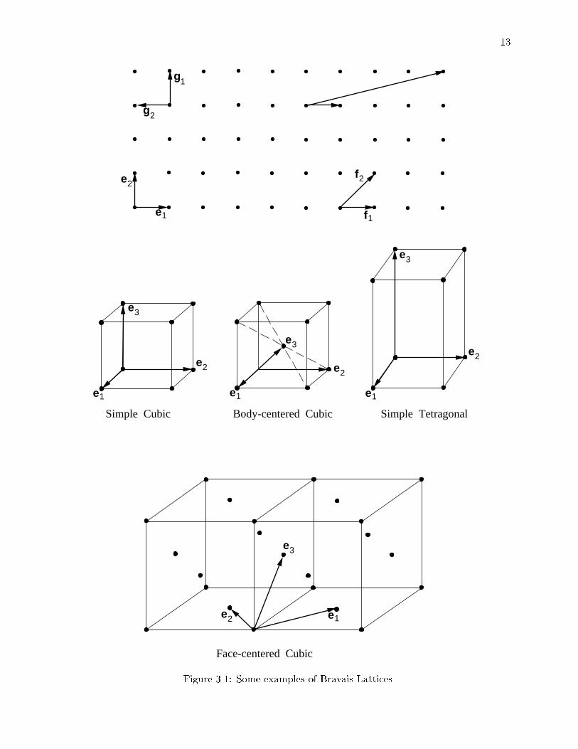
A Bravais lattice L(ei; o) is an innite set of points in three-dimensional space generated by thetranslation of a single point o through three linearly independent lattice vectors fe1; e2; e3g, i.e.,

L(ei; o) =nx : x = iei + o where 1; 2; 3 are integers:

o: (3.1)

Here we continue to use the summation convention: we sum any repeated indices so that iei =1e1 + 2e2 + 3e3. The lattice vectors fe1; e2; e3g dene an \unit cell". See Fig. 3.1 for a fewexamples.

Let us introduce some terminology that we will use later. It is conventional to denote a directionin a lattice by [uvw] where u, v and w are numbers. A comma or a space may or may not be usedto separate them. It denotes the direction given by the vector

d = ue1 + ve2 + we3: (3.2)

Fig. 3.2 shows a few examples on the left. It is conventional to write negative numbers usingan overhead bar. Notice that a direction remains unchanged if we multiply each of u, v andw with a positive constant, since the magnitude of the vector d is not important. A class ofcrystallographically equivalent directions is denoted by huvwi. For example, in a simple cubic latticewith lattice vectors chosen parallel to the edges, h100i = f[100]; [100]; [010]; [010]; [001]; [001]g.

It is conventional to denote a plane with its normal (hkl); once again h, k and l are numbers,a comma or a space may or may not separate them and a bar denotes a negative. To understandthis notation, it is necessary to introduce \reciprocal vectors". Dene vectors fe1; e2; e3g such that

ei ej =(

0 if i 6= j1 if i = j

for any i; j = 1; 2; 3: (3.3)

In other words, e1 is chosen to be perpendicular to e2 and e3 and its length is chosen such thate1 e1 = 1 and so on. See Fig. 3:3 for two examples. Notice that if the lattice vectors are mutuallyperpendicular, the reciprocal vectors are parallel to the lattice vectors. Now, the (hkl) plane is theplane with normal

n = he1 + ke2 + le3 (3.4)

Fig. 3.2 shows a few examples on the right. Once again the magnitude of the vector n as well asthe sense (+ or ) is not meaningful; therefore, the plane remains unchanged if we multiply eachof h, k and l with a constant. Finally, fhklg denotes a class of equivalent planes. For example,f110g = f(110); (110); (101); (101); (011); (011)g in a simple cubic lattice.

If each of u, v and w are rational numbers (ratio of integers like 12 , but not

p2), it is possible

to multiply them with the smallest common multiple of the denominators and express each as aninteger. Then, the direction is called a rational direction. These are exactly those directions thatgo through lattice points. Similarly a rational plane is one where h, k and l may be expressed asintegers. These are exactly those planes on which it is possible to nd a net or a two-dimensionalsub-lattice. A note of warning is worth bearing in mind while using this terminology. In practice,

13

g

g

f

f

e

e1

2

1

2

1

2

e3

e2 e1

e1

e2

e3

e1 e1

e2 e2

e3

e3

Simple Cubic Body-centered Cubic Simple Tetragonal

Face-centered Cubic

Figure 3.1: Some examples of Bravais Lattices.

14

[120]

[111]

[120]

(121)(111)

(121)

Figure 3.2: Some directions (left) and planes (right) in a lattice.

e2

e1

e1

e2

L

1/L

e2

e1e1 =

e2

1

Figure 3.3: Two examples of reciprocal basis.

15

one can measure directions (or planes) only up to a nite accuracy and consequently u, v and w(h, k and l) may be each be approximated by an integer within the accuracy of the measurement.Therefore, in practice, a rational direction (plane) typically denotes one where u, v and w (h, k andl) may be reduced to small integers where as an irrational direction (plane) denotes those wherethey can not.

3.2 Deformation of Lattices and Symmetry

Consider two Bravais lattices L(ei; o) and L(fi; o) generated by lattice vectors feig and ffig re-spectively. There is a matrix F with detF 6= 0 such that

fi = Fei: (3.5)

Therefore, we may regard, the lattice L(fi; o) as a deformation of the lattice L(ei; o) through F.There are some deformations which map a Bravais lattice back to itself. This is a consequence

of the symmetry in a lattice. For example, see the lattice at the top in Fig. 3.1 and consider theshear which maps feig to ffig. Notice that this shear maps the lattice back to itself. Similarly,notice that the rotation which maps feig to fgig in the same gure also maps the lattice back toitself. In order to understand the set of all deformations that map a lattice back to itself, we needthe following result.

Result 3.1. Two sets of lattice vectors fe1; e2; e3g and ff1; f2; f3g generate the same lattice, i.e.,L(ei; o) = L(fi; o), if and only if

ei = ji fj (3.6)

for some3 3 matrix of integers j

i such that det jj ji jj = 1: (3.7)

We have used the summation convention in Eq. (3.6) so that it actually represents three equations

ei = 1i f1 + 2

i f2 + 3i f3 i = 1; 2; 3: (3.8)

For example, take feig and ffig shown in the Fig. 3.1. It is easy to verify that they are relatedas

f1 = e1; f2 = e1 + e2; f3 = e3: (3.9)

Therefore,

jj ji jj =

0B@ 1 0 0

1 1 00 0 1

1CA : (3.10)

Similarly, feig and fgig in Fig. 3.1a are related through

jj ji jj =

0B@ 0 1 01 0 00 0 1

1CA : (3.11)

Using this result, we see that a matrix H maps the lattice back to itself if and only if

Hei = ji ej (3.12)

16

°e1

e2

e1

e = Fe

e = Fe

e = Fe

F = ∇ y(x)

°12

3

°°

1

2

3

e2°

yx y(x)

Figure 3.4: Lattice-continuum link using the Cauchy-Born Hypothesis. The lattice vectors deformaccording to the deformation gradient.

for some ji satisfying Eq. (3.7). Therefore, the set of deformations that map a lattice back into

itself is given by

G(ei) =nH :Hei = j

i ej for some ji satisfying Eq. (3.7)

o: (3.13)

G(ei) is a group and we call it the symmetry group of the lattice.This set G(ei) contains both shears and rotations as we saw earlier. However, notice that the

shears cause large distortions of the lattice and are associated with plasticity and slip. On the otherhand, rotations do not distort the lattice (see Section 2.2.3 for a precise meaning of distortion).In martensitic phase transformations, especially those in shape-memory alloys, plasticity is verylimited. Therefore, we would like to exclude these large shears by dening a smaller group.

The point group P is the set of rotations1 that map a lattice back to itself:

P(ei) =nR : R is a rotation and Rei = j

i ej for some ji satisfying Eq. (3.7)

o: (3.14)

For example, the point group of a simple cubic lattice is the group of 24 rotations that map theunit cube back to itself. It is easy to verify that the point group depends on the lattice and noton the particular choice of lattice vectors. It can be shown that there are only 11 distinct pointgroups which may be divided into 7 symmetry types.

3.3 Lattice-Continuum Link: The Cauchy-Born Hypothesis

We have so far been been discussing the lattice. Our goal, however, is to obtain a continuumtheory. Therefore, it is time to link the lattice picture to the continuum picture. We do so using

1Usually point groups include rotations and re ections. However, only the rotations play a role in a continuumtheory which we will soon develop and hence we conne ourself to rotations in this denition.

17

the Cauchy-Born hypothesis [18]. This is explained pictorially in Fig. 3.4. Consider a crystallinesolid. Let it occupy a region in the reference conguration. Assume that at each point x 2 ,there is a Bravais lattice with lattice vectors feoi (x)g. Conceptually, one can think of this as pickinga point in the body and then looking at it using some high powered microscope. Now suppose thatthe solid undergoes some deformation y(x) perhaps due to the application of some force or due toa change in temperature. Let F(x) be the deformation gradient. Now look at the lattice at thesame material point x after deformation. It is likely that it is distorted; so let fei(x)g be the latticevectors of this deformed lattice. The Cauchy-Born hypothesis says that the lattice vectors deformaccording the deformation gradient:

ei(x) = F(x) eoi : (3.15)

In other words, the lattice vectors behave like \material laments".

3.4 Energy Density in Crystalline Solids

Let us go back to our Bravais lattice L(ei; o). We assume that the Helmholtz free energy densityor simply the stored energy density of this lattice at a temperature is given by

'(ei; ) (3.16)

In other words, we assume that the energy density depends on the lattice vectors and the temper-ature. We require that the energy density satisfy two properties.

1. Frame-indierence. We assume that a rigid rotation of the lattice, or a change of frame, doesnot change the free energy density:

'(Qei; ) = '(ei; ) for all rotations Q: (3.17)

2. Material symmetry. We already know that more than one set of lattice vectors can describethe same Bravais lattice. We assume that the free energy density does not depend on thechoice of lattice vectors. In other words, two sets of lattice vectors that generate the samelattice must have the same free energy density:

'( ji ej ; ) = '(ei; ) for all j

i that satisfy Eq. (3.7) : (3.18)

We now use the Cauchy-Born hypothesis to obtain a continuum energy density. Let us choosea reference conguration and subject it to a deformation. We know that lattice vectors deformaccording to the deformation gradient. Therefore, we obtain a continuum free energy density'(F; ) from Eq. (3.16) by setting

'(F; ) = '(Feoi ; ): (3.19)

Since we dene the ' through ', it inherits all important properties of '.

1. Frame-indierence. It follows from Eq. (3.19) and Eq. (3.17) that

'(QF) = '(F) for all rotations Q: (3.20)

Therefore, a rigid-body rotation or a change in observer does not change the energy.

18

2. Material Symmetry. It follows from Eq. (3.19) and Eq. (3.18) that

'(FR; ) = '(F; ) for all rotations R 2 P(eoi ): (3.21)

Before we look at the derivation, let us understand this equation. It simply says that thecontinuum free energy should re ect the fact that the properties of a crystalline solid areidentical in crystallographically equivalent directions. Consider the following experiment.Take a reference crystal, deform it and look at its energy '(F). Now, rotate the referencecrystal through R and then apply the identical deformation. The corresponding deformationgradient is FR and the energy density is '(FR). If R is an element of the point group, therotated crystal is identical to the reference crystal; so the energy must be the same in bothexperiments or '(FR) = '(F).

For future use, we also note that we can combine this with frame-indierence Eq. (3.20) toobtain

'(RTFR; ) = '(F; ) for all rotations R 2 P(eoi ): (3.22)

At times it is convenient to use this, rather than Eq. (3.21) as the statement of materialsymmetry.

We now turn to the derivation of Eq. (3.21). This is easy though long, successively using Eq.(3.19), Eq. (3.16) and Eq. (3.18):

'(F; ) = '(F(x)eoi ; )= '(ei; )

= '( ji ej ; )

= '( ji Fe

oj ; )

= '(F( ji e

oj); )

= '(FHeoi ; )= '(FH; )

(3.23)

for all H in G(eoi ). However, we are interested in deformations that are small compared tolattice shears. Therefore, we conne H to the point group P(eoi ), rather than G(eoi ), to obtainEq. (3.21). This nal step is rather subtle and follows from a very nice result due to Pitteri[19] (also see [15, 20, 21, 22]).

3.5 Multi-Lattice

Consider the lattices shown in Fig. 3.5. Notice that neither can be described as a Bravais lattice.However, notice that each can be described as a collection of two identical or congruent Bravaislattices which are \shifted" from one another. In fact, any lattice can be described as a a collectionof a nite number (+1) of congruent Bravais lattices. Following Pitteri [23], we call such a latticea ( + 1)lattice or multi-lattice1. For simplicity, we will conne our discussion here to 2-lattices.The main ideas should be clear from this and the extension to the general case is conceptuallystraight-forward [23].

We describe a 2-lattice using three linearly independent lattice vectors fe1; e2; e3g and onevector p which we call shift. The lattice vectors describe the Bravais lattice and the shift describesthe oset or shift between the Bravais lattices:

L(ei;p; o) = L(ei; o)SL(ei; o+ p)

=x : x = iei + p+ o where 1; 2; 3 are integers and = 0 or 1

:

(3.24)

1Some books call a Bravais lattices simply a \lattice" and a multi-lattice a \crystal".

19

Two sets of lattices vectors and shift generate the same 2-lattice i.e., L(ei;p; o) = L(ei;q; o) if

ei = ji fj and q = iei + p (3.25)

where ji satises Eq. (3.7); i are any three integers and

=

(1 if the two Bravais lattices contain like atoms+1 if the two Bravais lattices contain unlike atoms

:

(3.26)

Given a 2-lattice L(ei;p; o), we dene the point group, P(ei;p) as the set of rotations that mapthe lattice back to itself:

P(ei;p) =(R 2 SO(3) :

Rei = j

i fjRp = iei + p

!for some j

i ; i; satisfying Eq. (3.26)

):

(3.27)The point group of the 2-lattice is smaller than or equal to the point group of the constituentBravais lattice; for example, see the lattice at the bottom of Fig. 3.5. The Bravais lattice is asquare lattice which is invariant under 90o rotations; but the 2-lattice is not.

We use the Cauchy-Born hypothesis to link the lattice and the continuum points of view.Consider a crystalline solid which undergoes a deformation y(x). Suppose the lattice vectors andshift at the material point x in the reference and deformed congurations are feoi ;pog and fei;pgrespectively. Then, the Cauchy-Born hypothesis says that the lattice vectors deform according tothe deformation gradient:

ei(x) = F(x)eoi : (3.28)

However, it does not relate the change in the shifts to the continuum deformation. In other words,each constituent Bravais lattice deforms according to continuum deformation, but their relativemovement is not related to the continuum deformation.

We assume that the Helmholtz free energy density of multi-lattice depends on the lattice vectors,shift and temperature and is given by

~'(ei;p; ): (3.29)

In the subsequent sections, we will study a theory in which we will minimize the total energy ofa crystalline body subject to some boundary conditions. However, according to the Cauchy-Bornhypothesis, the shifts are not linked to the continuum deformation. Therefore, the shift adjustsitself locally in order to minimize the energy for any given deformation and we can minimize theshifts out of the problem [24]. For any set of lattice vectors feig and any temperature , let ~p(ei; )be a shift that minimizes the energy density ~'. Let

'(ei; ) = ~'(ei; ~p(ei; ); ): (3.30)

This is the energy density of the lattice after we have minimized with respect to the shift. Noticethat this is identical to the energy density of the Bravais lattice discussed in Sec 3.4 and we proceedas before.

In summary, we can ignore the shifts by minimizing them out of the problem. The goodagreement between experiments in shape-memory alloys most of which are multi-lattices and thetheoretical predictions that we will see in the subsequent chapters shows that this is quite sat-isfactory when we are studying static microstructure using a framework of energy minimization.However, the shifts can have a profound eect in metastable and dynamic problems (see for example[24, 25, 26]).

20

e2

e1

qf2

f1

e2

e1

q

f1

f2

p

p

Figure 3.5: Two examples of multi-lattices.

4 Martensitic Phase Transformation

We are interested in developing a continuum theory for materials that undergo the martensiticphase transformation. In particular, we are interested in understanding the origin and the natureof the microstructure that is observed in these materials. In this section, we introduce the basicconcepts of the theory. We conne ourselves for now to specimens that are single crystals in theaustenite state. We describe dierent states of this specimen using deformations. The total energyof a specimen subjected to a deformation y at a temperature is given by

Z'(ry; )dV: (4.1)

Here ' is the stored energy density (or the Helmholtz free energy density). We assume thatit depends on the local distortion in the lattice measured by the deformation gradient and thetemperature following the discussion in Sec. 3.4. Our basic modeling postulate is the following:the specimen will occupy the state that minimizes this total energy. Therefore, the behavior of thespecimen - including its microstructure - is completely determined by the energy density '. In this

21

e3

e2 e1a

a°

a°a

a

(a)

a

a

c

e1m

e2m

e3m

(b)

a°1 3

2

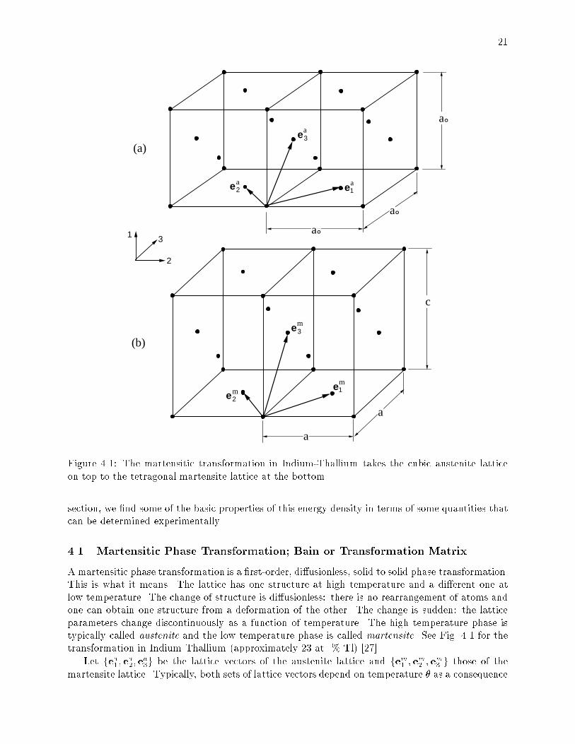
Figure 4.1: The martensitic transformation in Indium-Thallium takes the cubic austenite latticeon top to the tetragonal martensite lattice at the bottom.

section, we nd some of the basic properties of this energy density in terms of some quantities thatcan be determined experimentally.

4.1 Martensitic Phase Transformation; Bain or Transformation Matrix

A martensitic phase transformation is a rst-order, diusionless, solid to solid phase transformation.This is what it means. The lattice has one structure at high temperature and a dierent one atlow temperature. The change of structure is diusionless: there is no rearrangement of atoms andone can obtain one structure from a deformation of the other. The change is sudden: the latticeparameters change discontinuously as a function of temperature. The high temperature phase istypically called austenite and the low temperature phase is called martensite. See Fig. 4.1 for thetransformation in Indium Thallium (approximately 23 at. % Tl) [27].

Let fea1; ea2; ea3g be the lattice vectors of the austenite lattice and fem1 ; em2 ; em3 g those of themartensite lattice. Typically, both sets of lattice vectors depend on temperature as a consequence

22

of thermal expansion. However thermal expansion is much smaller than the distortion due totransformation in the range of temperatures that we are interested in. Therefore, we will neglect itin this presentation for simplicity. We point out that the presentation can be readily modied totake thermal expansion into account.

We can describe the transformation from the austenite lattice to the martensite lattice as adeformation because there is no diusion. Therefore, we can nd a matrix U1 such that

emi = U1eai : (4.2)

U1 describes the homogeneous deformation that takes the lattice of the austenite to that of themartensite. This is called the Bain matrix or the transformation matrix.

Consider for example the transformation in InTl [27] shown in Fig. 4.1. It undergoes a cubic

to tetragonal transformation. InTl is a disordered alloy (which means the Indium and Thalliumatoms are randomly distributed on the lattice), and we can describe it as a Bravais lattice both inthe austenite and the martensite phase. It has a face-centered cubic lattice in the austenite statewhile it has a face-centered tetragonal lattice in the martensite state. The lattice vectors of theaustenite and martensite are

ea1 =12f0; ao; aog; em1 = 1

2f0; a; ag;ea2 =

12f0;ao; aog; em2 = 1

2f0;a; ag;ea3 =

12fao; 0; aog; em3 = 1

2fc; 0; ag(4.3)

in an orthonormal basis parallel to the edges of the cubic unit cell. Therefore, it is easy to verifythat the transformation matrix is given by

U1 =

0B@ 0 0

0 00 0

1CA (4.4)

(where = a=a0 and = c=ao) with respect to the basis parallel to the edges of the cubic unit cell(see Fig. 4.1). In InTl, the quantities ao = 4:7445 A, a = 4:6919 A, c = 4:8451 A, so that = 0:9889and = 1:0221. There are many alloys which undergo a cubic to tetragonal transformation. Thetransformation matrix is always of the form shown in Eq. (4.4) where ; depend on the latticeparameters of the material. We will see some examples later.

Copper-Aluminum-Nickel (approximately 14 wt. % Al and 4 wt. % Ni) [28] undergoes acubic to orthorhombic transformation as shown in Fig. 4.2. CuAlNi is an ordered lattice and it issucient to look only at the copper atoms in order to describe the transformation. The latticeof copper atoms is face-centered cubic in the austenite state. The lattice in the martensite stateis almost body-centered orthorhombic; the atom at the center is slightly displaced away from thebody center. The transformation may be described as follows. Cut a body-centered tetragonal cellfrom two adjacent cubic austenite cells and then stretch it unequally along the three edges of thistetragonal cell to obtain the orthorhombic martensite cell. Therefore, notice the austenite lattice isstretched unequally along three mutually perpendicular directions: two of these are face-diagonalsof the cubic while the third is an edge. Therefore, the transformation matrix

U1 =

0BBBBBBBB@

+

20

2

0 0

20

+

2

1CCCCCCCCA

(4.5)

23

a°a°

a°

1

3

2

b

ca

Figure 4.2: The martensitic transformation in Copper-Aluminum-Nickel takes the cubic austenitelattice on the left to the orthorhombic martensite lattice on the right.

(where =p2a=ao, = b=a0 and =

p2a=ao) in an orthonormal basis parallel to the edges of

the cubic unit cell. In CuAlNi, the quantities ao = 5:836 A, a = 4:3823 A, b = 5:3563 A, c = 4:223A, so that = 1:0619; = 0:9178; = 1:0231. Notice that in this transformation, two of the threeaxes of orthorhombic symmetry are obtained from h110icubic axes. In any cubic to orthorhombictransformation where this is true, the transformation matrix is of the form shown in Eq. (4.5);; ; are obtained from the lattice parameters. We will see some other examples later.

There is another type of cubic to orthorhombic transformation here all the axes of orthorhom-bic symmetry are obtained from h100icubic axes. However, I do not know of any material thatundergoes such a transformation and hence we do not consider this case any further. Henceforth,a cubic to orthorhombic transformation will refer to the type of transformation in CuAlNi.

Before we proceed, there are two important points to keep in mind about the transformationmatrix. First, the transformation matrix describes the overall deformation of the lattice, but notnecessarily every atom in the lattice. Notice that the atom at the center of the martensite unitcell in CuAlNi shown in Fig. 4.2 does not follow the homogeneous deformation described by thetransformation matrix. In fact, we need to describe both the austenite and the martensite as multi-lattices (see Sec. 3.5) in order to fully describe the transformation in CuAlNi. The transformationmatrix describes the deformation of the lattice vectors, but not necessarily the shifts. Therefore,one should be very careful in choosing the lattice vectors of both the austenite and the martensitelattices in order to get an accurate description of the transformation. The correct choice is the onedened by the \lattice correspondence".

Second, the transformationmatrix obtained through Eq. (4.2) is symmetric in both the examplesabove. However, there are materials like NiTi where this is not so [29]. Instead, a matrix T1 whichis not symmetric satises

emi = T1eai : (4.6)

In such cases, we slightly modify the denition of transformation matrix. We use Procedure 2.2to decompose T1 = QU1 where Q is a rotation and U1 is positive-denite and symmetric. Wecall U1 (and not T1) the transformation matrix. Notice that T1 and U1 are related through a

24

e ia

(U )2 (I) 1(U )

θ > θ

θ = θ

θ < θ

°

°

°

e i

e im(F)

ϕ

Figure 4.3: The energy density at various temperatures.

rotation. According to the idea of frame-indierence, rotations do not change the state of a lattice,and hence this modication does not aect the development1. Therefore, we will assume in generalthat the transformation matrix is symmetric and positive-denite.

4.2 Energy Density

The austenite state is stable at high temperatures while the martensite state is stable at lowtemperatures. Therefore, the energy density ' introduced in Eq. (3.16) has the behavior shownschematically in Fig. 4.3. The austenite lattice vectors feai gminimizes it at high temperatures whilethe martensite lattice vectors femi g minimizes it at low temperatures. Therefore, there must be atemperature at which both feai g and femi g have equal energy. We will call this the transformation

1It is also possible to proceed without making this modication as in Bhattacharya [30].

25

temperature o. Therefore, we have

'(eai (); ) '(ei; ) > o'(eai (); ) = '(emi (); ) '(ei; ) = o'(emi (); ) '(ei; ) < o

(4.7)

for all lattice vectors ei.We now pass to the continuum theory using the Cauchy-Born hypothesis. Let us choose an

undistorted crystal of austenite at the transformation temperature as our reference conguration.Thus the reference lattice is the austenite lattice or eoi = eai . We invoke the Cauchy-Born hypothesis(see Fig. 3.4) and use the deformation gradient to identify the states of the body. Clearly, givenour choice of reference conguration, a deformation gradient equal to identity I corresponds to theaustenite state while a deformation gradient equal to the the transformation matrix or Bain matrixU1 corresponds to the undistorted martensite lattice. Therefore according to Eq. (3.19) and Eq.(4.7) the continuum energy density satises the following:

'(I; ) '(F; ) > o'(I; o) = '(U1; o) '(F; o) = o'(U1; ) '(F; ) < o

(4.8)

for all matrices F. This is also shown schematically in Fig. 4.3. Let us now examine the consequencesof frame-indierence and material symmetry on these equations.

4.3 Material Symmetry: Variants of Martensite

In the examples of InTl and CuAlNi that we saw above, the austenite lattice has greater symmetrythan the martensite lattice. This is the case in most martensitic transformations and shape-memoryalloys. We assume henceforth that the austenite has strictly greater symmetry than the martensite.Precisely, we will assume that the point group of the martensite Pm is a subgroup of the pointgroup of the austenite Pa. This assumption has very important consequences. In particular, itgives rise to symmetry related variants of martensite.

Let us go back to the example of InTl shown in Fig. 4.1. We chose to elongate the austenitelattice along one of the three cubic axes to obtain the martensite lattice. Instead, we could havechosen any of the other two. Then, we would once again obtain a tetragonal lattice; however, theorientation of this lattice would be dierent relative to the austenite lattice as shown in Fig. 4.4.We will call these the variants of martensite. The three variants of martensite in this case havetransformation matrices U1;U2 or U3 shown in Table 4.1.

Let us try to understand it in a more general setting, we can think of the example above asfollows. We rotate the austenite lattice through a rotation R in its point group Pa and thentransform it. This gives us a variant of martensite. Notice that the transformation matrix of thisvariant is RTU1R. Doing this for all the rotations R in Pa we obtain all the dierent variants ofmartensite. However, for some rotations R in Pa, it may turn out that RTU1R = U1. Indeed,this happens if R is also in the point group of the martensite Pm (for example, consider the 90o

rotation about the vertical axis in our example above). In such a case we do not obtain a dierentvariant. Thus,

the number of martensite variants, N =the number of rotations in Pathe number of rotations in Pm : (4.9)

(In the example of the cubic to tetragonal transformation,N = 24=8 = 3.) Further, letU1;U2; : : : ;UN

be the distinct matrices of the form RTU1R. These are the transformation matrices of the variants

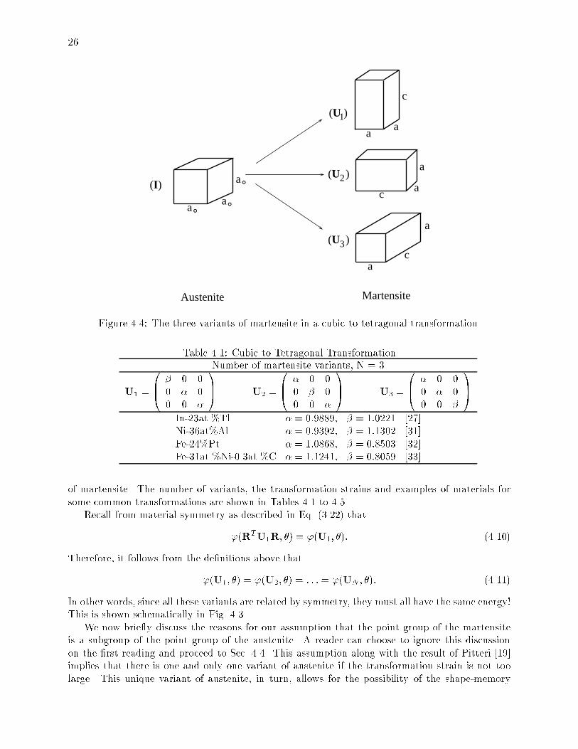
26

aa

c

c

a

a

a

a

c

a°a°a°

(I)

(U )1

(U )2

(U )3

Austenite Martensite

Figure 4.4: The three variants of martensite in a cubic to tetragonal transformation.

Table 4.1: Cubic to Tetragonal TransformationNumber of martensite variants, N = 3

U1 =

0B@ 0 0

0 00 0

1CA U2 =

0B@ 0 0

0 00 0

1CA U3 =

0B@ 0 0

0 00 0

1CA

In-23at.%Tl = 0:9889; = 1:0221 [27]Ni-36at%Al = 0:9392; = 1:1302 [31]Fe-24%Pt = 1:0868; = 0:8503 [32]Fe-31at.%Ni-0.3at.%C = 1:1241; = 0:8059 [33]

of martensite. The number of variants, the transformation strains and examples of materials forsome common transformations are shown in Tables 4.1 to 4.5.

Recall from material symmetry as described in Eq. (3.22) that

'(RTU1R; ) = '(U1; ): (4.10)

Therefore, it follows from the denitions above that

'(U1; ) = '(U2; ) = : : : = '(UN ; ): (4.11)

In other words, since all these variants are related by symmetry, they must all have the same energy!This is shown schematically in Fig. 4.3.

We now brie y discuss the reasons for our assumption that the point group of the martensiteis a subgroup of the point group of the austenite. A reader can choose to ignore this discussionon the rst reading and proceed to Sec. 4.4. This assumption along with the result of Pitteri [19]implies that there is one and only one variant of austenite if the transformation strain is not toolarge. This unique variant of austenite, in turn, allows for the possibility of the shape-memory

27

Table 4.2: Tetragonal to Orthorhombic TransformationNumber of martensite variants, N = 2

U1 =

0B@ 0 0

0 00 0

1CA U2 =

0B@ 0 0

0 00 0

1CA

YBa2Cu3O7 = 0:9898; = 1:0068 = 0:9887 [34]

Table 4.3: Cubic to Orthorhombic TransformationNumber of martensite variants, N = 6

U1 =

0BBBBBBBB@

+

20

2

0 0

2

0+

2

1CCCCCCCCAU2 =

0BBBBBBBB@

+

20

2

0 0

20

+

2

1CCCCCCCCAU3 =

0BBBBBBBB@

+

2

2

0

2

+

20

0 0

1CCCCCCCCA

U4 =

0BBBBBBBB@

+

2

20

2

+

20

0 0

1CCCCCCCCAU5 =

0BBBBBBBB@

0 0

0+

2

2

0

2

+

2

1CCCCCCCCAU6 =

0BBBBBBBB@

0 0

0+

2

2

0 2

+

2

1CCCCCCCCA

Cu-14.2wt%Al-4.3wt.%Ni = 1:0619; = 0:9278 = 1:0230 [28]Au-47.5%Cd = 1:0138; = 0:9491 = 1:0350 [35; 36]

Table 4.4: Cubic to Monoclinic-I TransformationNumber of martensite variants, N = 12

U1 =

0B@

1CA U2 =

0B@

1CA U3 =

0B@

1CA U4 =

0B@

1CA

U5 =

0B@

1CA U6 =

0B@

1CA U7 =

0B@

1CA U8 =

0B@

1CA

U9 =

0B@

1CA U10 =

0B@

1CA U11 =

0B@

1CA U12 =

0B@

1CA

Ni-50.6at.%Ti = 1:0243; = 0:9563 = 0:058 = 0:0427 [29]Note: There are two types of cubic to monoclinic transformations; in monoclinic-I, the axis ofmonoclinic symmetry corresponds to a h110icubic direction.

28

Table 4.5: Cubic to Monoclinic-II TransformationNumber of martensite variants, N = 12

U1 =

0B@ 0

00 0

1CA U2 =

0B@ 0 00 0

1CA U3 =

0B@ 0 00 0

1CA U4 =

0B@ 0 00 0

1CA

U5 =

0B@ 0

0 0 0

1CA U6 =

0B@ 0

0 0 0

1CA U7 =

0B@ 0

0 0 0

1CA U8 =

0B@ 0

0 0 0

1CA

U9 =

0B@ 0 0

0 0

1CA U10 =

0B@ 0 0

0 0

1CA U11 =

0B@ 0 0

0 0

1CA U12 =

0B@ 0 0

0 0

1CA

Cu-15at.%Zn-17at.%Al = 1:0101; = 1:0866 = 0:9093 = 0:0249 [37]Note: There are two types of cubic to monoclinic transformations; in monoclinic-II, the axis ofmonoclinic symmetry corresponds to a h100icubic direction.

eect as we will see in Sec. 9. On the other hand, a failure of this assumption leads to an an innitenumber of variants of both austenite and martensite. This is easily seen in the face-centered cubicto body-centered cubic transformation in say pure Iron. We obtain such a transformation if weset a

c=p2 in the cubic to tetragonal transformation in Fig. 4.1. Let us start from an fcc lattice

and transform to a bcc lattice; as discussed earlier, we can do so in three equivalent ways. Let uschoose one. We can transform back to an fcc lattice by elongating an edge of the bcc unit cell however, we nd that there are three equivalent ways of doing so. One of the three ways bringsus back to the fcc lattice that we started from; but the other two do not bring us back, insteadthey take us to other fcc lattices. But each of these in turn have three equivalent bcc lattices andso on. We thus nd that there are an innite number of symmetry-related fcc and bcc lattices oran innite number of fcc and an innite number of bcc variants. This has serious consequences asa sequence of forward and reverse transformation can lead to strains as we go from one variant ofaustenite to another. Indeed, fcc twins are observed in some ferrous alloys that undergo a fcc tohcp transformation [38]; these twins reveal the fact that there are more than one variants of thefcc austenite. This is in fact one of the diculties in making a good ferrous shape-memory alloy.Further, a theory based on energy minimization is quite unsatisfactory in a situation when one hasan innite number of variants [39].

4.4 Frame Indierence: Energy Wells

Consider a crystal in the austenite state and rotate it. It continues to remain in the austenite state.In other words, a rigid rotation does not change the state of the crystal. Therefore, the austenitecorresponds not only to the identity matrix I, but to all rotation matrices Q. Similarly, the rstvariant of martensite corresponds to all matrices of the form QU1 where Q is a rotation and so on.

29

N QU

NU

3U

QU3

QU

1

Q

U

I

1

2U

QU2

Figure 4.5: The energy wells. Consider the plane of the paper to be the space of all matrices.The circles schematically represent pre-multiplication with all rotations. The dashed circle is theaustenite well and the rest are the martensite wells.

Therefore, let us dene

A = fF : F = Q for some rotation Qg ;M1 = fF : F = QU1 for some rotation Qg ;M2 = fF : F = QU2 for some rotation Qg ;

...MN = fF : F = QUN for some rotation Qg :

(4.12)

The set A consists of all matrices that correspond to the austenite and we call it the austenite

well. This is shown schematically in Fig. 4.5 as a circle. Similarly, MI consists of all matrices thatcorrespond to the Ith variant of martensite. We call it the Ith martensite well. Finally, let M bethe collection of all martensite wells:

M =M1

[M2

[: : :[MN (4.13)

These are also shown in Fig. 4.5.

Since a rigid rotation does not change the state of a crystal, it does not change the energy. This

30

Q QU

U

R U RTU

R

RT

Figure 4.6: The dierence between rotations that are considered in frame-indierence and materialsymmetry.

is the idea of frame-indierence as described in Eq. (3.20). Therefore,

'(QI; ) = '(I; )'(QU1; ) = '(U1; )

...'(QUN ; ) = '(UN ; )

(4.14)

for all rotations Q. In other words, all matrices in a given well have the same energy.Finally, it is worth clarifying one important point. Both material symmetry and frame-indierence

involve rotations. However, the way they act is very dierent. This is shown in Fig. 4.6. Let U bea stretch in the vertical direction and Q = R be a clockwise rotation of 90o. Notice the dierencebetween QU and RTUR. In material symmetry, the rotation acts in the reference congurationand in frame-indierence, the rotation acts in the deformed conguration. Therefore, it is notpossible to rigidly rotate one variant to obtain another. In other words, it is not possible to nd arotation Q such that QU1 = U2. This would violate the uniqueness aspect of the polar decompo-sition theorem. Therefore, the energy wells dened in Eq. (4.12) are indeed disjoint, i.e. they donot intersect each other.

4.5 Summary of the Energy Density

Let us now put all of this together. We use the lattice correspondence and the lattice parameters tond the transformation matrix U1. Using the polar decomposition theorem if necessary, we ensurethat this matrix is symmetric and positive-denite. We then nd the transformation strains of thedierent variants of martensite as the distinct matrices U1;U2; : : :UN of the form RTU1R whereR is a rotation in the point group of the austenite Pa. The number of variants N depends onthe change in symmetry and is given by Eq. (4.9). It important to emphasize that for any givenmaterial, the number of variants as well as the transformation is completely determined by thelattice structures of the austenite and the martensite and can be determined experimentally.

Having determined these, we can say the following about the energy. According to materialsymmetry, Eq. (4.10), all the variants have the same energy. According to frame-indierence theaustenite and the variants of martensite are described by wells, Eq. (4.12). Putting these togetherwith Eq. (4.8), we can say the following about the behavior of the energy density. The energy

31

density ' is minimized on the austenite well A at high temperatures, it is minimized on themartensite wells M at low temperatures and on both the austenite and the martensite wells M atthe transformation temperature o:

'(G; ) '(F; ) for all G 2 A and for all F > o'(G; ) '(F; ) for all G 2 ASM and for all F = o'(G; ) '(F; ) for all G 2 M and for all F < o:

(4.15)

Therefore, if we are looking for energy minimizing congurations of our specimen, we should lookfor deformations y where the deformation gradient ry belong to the relevant energy wells.

4.6 Multiple Transformations

In certain compositions, NiTi transforms from the cubic austenite to a rhombohedral \R-phase"before transforming to the martensite. In such a transformation, we will use the austenite stateas the reference conguration for both transformations [30]. Thus, we have two transformationmatrices, UR

I which describes the deformation from the austenite to the R-phase and UmI which

describes the deformation from the austenite to the martensite. We calculate the number of variantsof the R-phase using Eq. (4.9) with the point group of the austenite and the point group of theR-phase this gives us 24=6 = 4 variants. We calculate the number of variants of the martensiteusing Eq. (4.9) with the point group of the austenite and the point group of the martensite thisgives us 24=2 = 12 variants. We just use the relevant wells depending on the temperature of ourinterest. The alternative approach of treating these two transformations separately requires changesof reference conguration; this is rather laborious and can easily lead to incorrect conclusionsconcerning the symmetry.

5 Twinning in Martensite

In this section, we study a very important energy minimizing deformation twins in the marten-site. The purpose is two-fold. First, it gives a glimpse of the richness of the energy minimizingdeformations in these martensitic materials. Second, it shows that the possible twinning modes inthe martensite are determined as a consequence of the energy well structure. In other words, inthis theory, one does not need to know the twinning modes a priori; instead, they are obtained asa result.

5.1 Deformation Involving Two Variants

Let us begin by trying to nd a deformation which involves two wells, say those correspondingto variants I and J of the martensite. In other words, we are looking for a deformation y of thetype shown in Fig. 5.1a: the deformation gradient is in the Ith martensite well MI in one part ofthe body 1 and in the Jth martensite well MJ in the other part of the body 2. Recalling thestructure of the energy wells from Eq. (4.12), we seek a deformation y such that

ry =

8><>:Q1UI in 1

Q2UJ in 2

for some rotations Q1;Q2. (5.1)

Remark 5.1. Notice that we have taken the rotations Q1 and Q2 to be constant. It appearsthat we would obtain a more general deformation involving these two variants if we assume that

32

n

y = Q U1 I y = Q U2 J

MartensiteVariant I

MartensiteVariant J

Q U1 I

Q U2 J

UI UJ

(a) (b)

Figure 5.1: (a) A deformation with two variants or a twin. (b) Schematic representation of a twin.

they are functions of x. However, this is not possible and the constant rotation is the most generalsituation. To understand this, consider a smooth deformation y with ry(x) = Q(x), or

Qij =@yi@xj

: (5.2)

Therefore, the equality of second derivatives requires

@Qij

@xk=@Qik

@xj: (5.3)

It is easy to show appealing to the fact that Q(x) is a rotation that the only possibility consistentwith this equation is Q = constant. This argument can also be generalized to non-smooth defor-mations [40]. In some sense, this is equivalent to the statement that bodies can not bend with zerodistortion. Thus, the deformation shown in Eq. (5.1) is the most general deformation involving twowells.

Clearly, the deformation gradient suers a jump in this deformation and we have to satisfy thekinematic compatibility condition described in Eq. (2.31), or

Q1UI Q2UJ = b n (5.4)

for some vectors b and n. Furthermore, the interface between the two regions is necessarily a planewith normal n in the reference conguration.

Fig. 5.1b is a schematic representation of this deformation. We join two matrices with a straightline if they can form an interface between them. Recall from Fig. 4.5 that we represent the energywells as circles. Q1UI and Q2UJ are the matrices on the Ith and Jth martensite wells respectively.Since they satisfy the condition Eq. (5.4), they can form an interface; we show this by joining themwith a straight line.

Premultiplying this equation by QT2 and setting Q = QT

2Q1 and a = QT2 b, we can rewrite Eq.

(5.4) asQUI UJ = a n: (5.5)

We call this the twinning equation anticipating the interpretation that follows.

33

5.2 Interpretation as a Twin

A twin is a visible coherent interface in a crystal which satises the following1:

1. The lattice on one side can be obtained by a simple shear of the lattice on the other.

2. The lattice on one side can also be obtained by a rotation of the lattice on the other.

We now show that the deformation described in Sec. 5.1 can be interpreted as a transformationtwin involving variants I and J . Let ffig, fgig be the lattice vectors on the two sides of theinterface. According to the Cauchy-Born hypothesis,

fi = QUIeai and gi = UJe

ai (5.6)

where feai g are the lattice vectors of the reference austenite lattice. According to Eq. (5.5),

QUI = (UJ + a n) = (I+ a (U1J n))UJ : (5.7)

Operating this on eai and using Eq. (5.6), we obtain

fi = (I+ a (U1J n))gi (5.8)

But (I + a (U1J n)) is a simple shear. This is seen by taking the determinant of Eq. (5.7) andusing a result from matrix algebra,

detUI = det(QUI) = det(I+ a (U1J n)) detUJ = (1 + a (U1J n)) detUJ : (5.9)

However, detUI = detUJ and it follows that a (U1J n) = 0. Therefore, (I + a (U1J n)) is asimple shear and Eq. (5.8) says that the lattice vectors on one side can be obtained by a simpleshear of the other side, satisfying the rst requirement.

To see the second, recall that UI is related to UJ by some rotation R in the point group of theaustenite Pa:

UI = RTUJR where R is a rotation that satises Reai = jie

aj (5.10)

for some ji consistent with Eq. (3.7). Therefore,

fi = QUIeai = QRTUJRe

ai = QRTUJ

jie

aj = jiQR

TUJeaj = jiQ

0gj (5.11)

where Q0 = QRT is a rotation. Therefore, the lattice vectors ffig and fQ0gig describe the samelattice according to Theorem 3.1. In other words, a rotation of fgig gives lattice vectors which arecrystallographically equivalent to ffig. Thus, we satisfy the second requirement and the deformationin Sec. 5.1 describes a twin.

The twinning elements the twinning shear s, the direction of shear 1 and the shearing plane(relative to the lattice on one side) K1 are given by

s = jaj jU1J nj; 1 =a

jaj ; K1 =U1J n

jU1J nj : (5.12)

1There are many denitions of a twin [41, 42, 43, 44]; we have chosen one which is most convenient for our purpose.

34

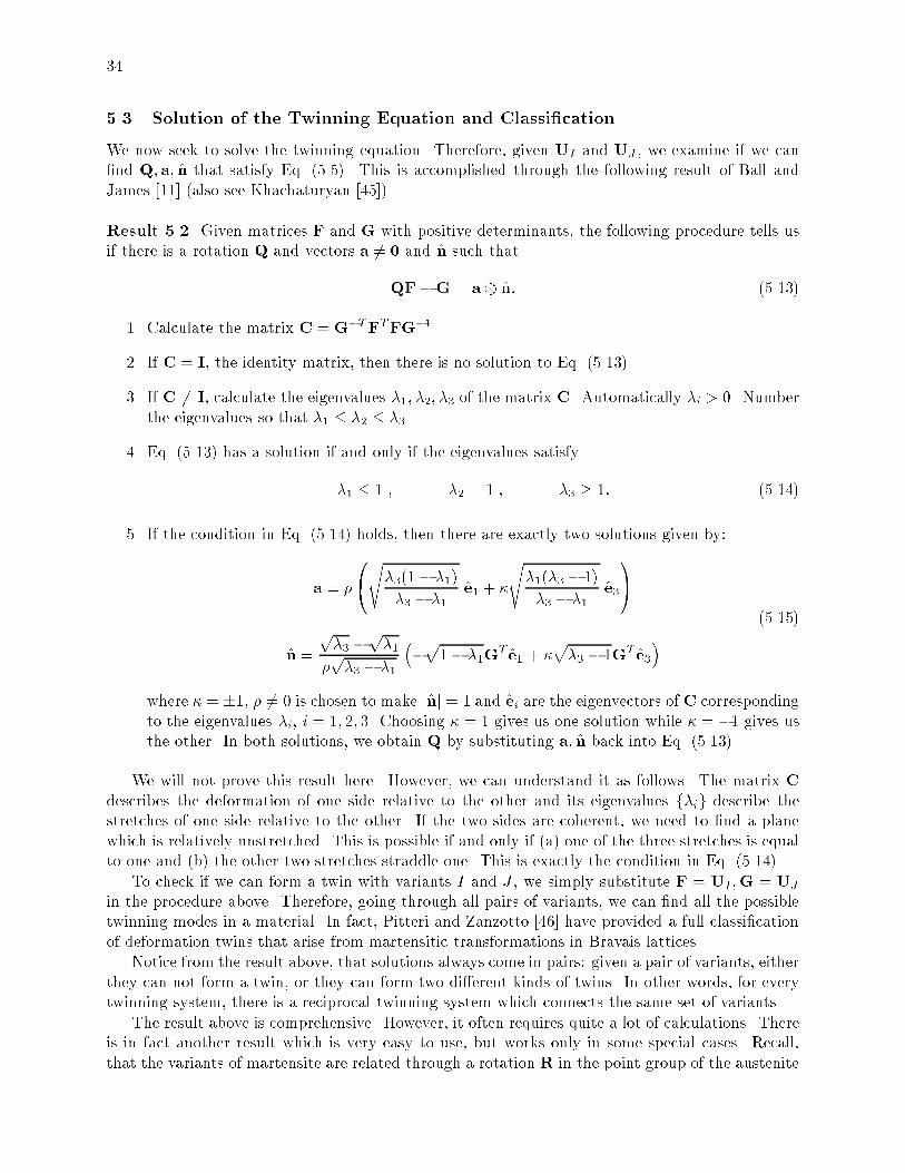
5.3 Solution of the Twinning Equation and Classication

We now seek to solve the twinning equation. Therefore, given UI and UJ , we examine if we cannd Q; a; n that satisfy Eq. (5.5). This is accomplished through the following result of Ball andJames [11] (also see Khachaturyan [45]).

Result 5.2. Given matrices F and G with positive determinants, the following procedure tells usif there is a rotation Q and vectors a 6= 0 and n such that

QFG = a n: (5.13)

1. Calculate the matrix C = GTFTFG1.

2. If C = I, the identity matrix, then there is no solution to Eq. (5.13).

3. If C 6= I, calculate the eigenvalues 1; 2; 3 of the matrix C. Automatically i > 0. Numberthe eigenvalues so that 1 2 3.

4. Eq. (5.13) has a solution if and only if the eigenvalues satisfy

1 1 ; 2 = 1 ; 3 1: (5.14)

5. If the condition in Eq. (5.14) holds, then there are exactly two solutions given by:

a =

0@s3(1 1)3 1

e1 +

s1(3 1)

3 1e3

1A

n =

p3

p1

p3 1

p1 1G

T e1 + p3 1GT e3

(5.15)

where = 1, 6= 0 is chosen to make jnj = 1 and ei are the eigenvectors of C correspondingto the eigenvalues i, i = 1; 2; 3. Choosing = 1 gives us one solution while = 1 gives usthe other. In both solutions, we obtain Q by substituting a; n back into Eq. (5.13).

We will not prove this result here. However, we can understand it as follows. The matrix Cdescribes the deformation of one side relative to the other and its eigenvalues fig describe thestretches of one side relative to the other. If the two sides are coherent, we need to nd a planewhich is relatively unstretched. This is possible if and only if (a) one of the three stretches is equalto one and (b) the other two stretches straddle one. This is exactly the condition in Eq. (5.14).

To check if we can form a twin with variants I and J , we simply substitute F = UI ;G = UJ

in the procedure above. Therefore, going through all pairs of variants, we can nd all the possibletwinning modes in a material. In fact, Pitteri and Zanzotto [46] have provided a full classicationof deformation twins that arise from martensitic transformations in Bravais lattices.

Notice from the result above, that solutions always come in pairs: given a pair of variants, eitherthey can not form a twin, or they can form two dierent kinds of twins. In other words, for everytwinning system, there is a reciprocal twinning system which connects the same set of variants.

The result above is comprehensive. However, it often requires quite a lot of calculations. Thereis in fact another result which is very easy to use, but works only in some special cases. Recall,that the variants of martensite are related through a rotation R in the point group of the austenite

35

Pa: UI = RTUJR. If this rotation R is a 180o rotation, then Eq. (5.5) has solutions and they canbe obtained very easily through the following result [47, 48, 49, 50].

Result 5.3. Suppose R is a 180o rotation about some axis e and the matrices F and G satisfy

1: F = QGR for some rotation Q, or equivalently, FTF = RTGTGR

2: FTF 6= GTG(5.16)

Then, there are two solutions to Eq. (5.13) and they are

1: a = 2

GT ejGT ej2 Ge

!; n = e

2: a = Ge ; n =2

e GTGe

jGej2! (5.17)

where 6= 0 is chosen to make jnj = 1. In both solutions, we obtain Q by substituting a; n backinto Eq. (5.13).

It is easy to verify Result 5.3 using the representation R = I + 2e e for a 180o rotation.

Note that this result is not comprehensive. The failure of condition Eq. (5.16) does not rule outa solution. Therefore, if this condition is not satised, we have to use Result 5.2 to check if thereare any solutions.

This result tells us that a lost element of two-fold symmetry a 180o rotation which is in Pa butnot in Pm gives rise to a twinning system in the martensite. This is often called Mallard's law.Most twins in the martensite are of this kind, but there are exceptions as pointed out by Simha[51] as well as Pitteri and Zanzotto [46].

This Result 5.3 allows us to classify the twins. Notice in the rst solution, Eq. (5.17)1, thetwinning plane is a plane of symmetry in the austenite. Therefore, this plane is rational and thissolution describes a Type I twin. Next, notice that the shearing direction in the second solution,Eq. (5.17)2 is a direction of symmetry in the austenite and hence rational. Therefore, this solutiondescribes a Type II twin. Finally, there are occasions in which there are two 180o rotations thatsatisfy Eq. (5.16); call them R1 and R2. Thus, it appears that Result 5.3 gives us four solutionsto the twinning equation: two using R1 and two using R2. However, Result 5.2 tells us that therecan be at most two solutions. It turns out that the Type I solution Eq. (5.17)1 using R1 coincideswith the Type II solution Eq. (5.17)2 using R2 and vice-versa. Consequently, there are only twosolutions. However, each solution can be described as both a Type I and a Type II twin and boththe twinning plane and shearing direction are rational. These are called Compound twins.

5.4 Twins in a Cubic to Tetragonal Transformation

Let us now nd all the possible twins in a cubic to tetragonal transformation. We begin withvariants 1 and 2. Let R be a 180o rotation about e = 1p

2f1; 1; 0g. It is easy to verify that

RTU1R = U2. Therefore, these matrices satisfy Eq. (5.16) for F = U2;G = U1 and these twovariants are related by a twin according to Result 5.3. The solutions to the twinning equationare given by Eq. (5.17). Substituting e;G in this equation, a little calculation shows that the two

36

solutions are

1: a =

p2(2 2)2 + 2

f; ; 0g n =1p2f1; 1; 0g

2: a =

p2(2 2)2 + 2

f;; 0g n =1p2f1;1; 0g

(5.18)

in the cubic basis. It turns out that these two variants also satisfy Eq. (5.16) for the 180o rotationabout the axis 1p

2f1;1; 0g. This rotation also gives us the same solutions. Therefore, we conclude

that these twins are compound. Similarly, if we pick variants 1 and 3, we nd that they satisfy Eq.(5.16) with 180o rotations about 1p

2f1; 0;1g. Therefore they can also form twins and the solution

can obtained by switching the 2 and the 3 components in Eq. (5.18). Finally, variants 2 and 3 arealso twin-related and the solution is obtained by switching the 1 and the 3 components in equationEq. (5.18).

Thus each pair of variants in a cubic to tetragonal transformation can form a twin. Further, allthe twins are compound and the twin planes are f110gcubic.

5.5 Twins in a Cubic to Orthorhombic Transformation

We now nd all the possible twins in a cubic to orthorhombic transformation. Let us begin withvariants 1 and 2. Let R be a 180o rotation about e = f1; 0; 0g. It is easy to verify that RTU1R =U2. So these matrices satisfy the Eq. (5.16) for F = U2;G = U1. Therefore, these two variantsare related by a twin according to Result 5.3 and we can nd the solution to the twinning equationusing Eq. (5.17). Substituting e;G in this equation, a little calculation shows that the two solutionsare

1: a = 2 2

2 + 2f( ); 0; (+ )g n = f1; 0; 0g

2: a = 2 2 2 + 2

f(+ ); 0; ( )g n = f0; 0; 1g(5.19)

in the cubic basis. It turns out that these two variants also satisfy Eq. (5.16) for the 180o rotationabout the axis f0; 0; 1g. This rotation also gives us the same solutions. Therefore, these twins arecompound.

Now consider variants 1 and 3. It is easy to verify that RTU1R = U3 where R is a 180o

rotation about e = 1p2f1; 0; 1g. Therefore, these matrices satisfy Eq. (5.16) for F = U3;G = U1

and we can nd the solution to the twinning equation using Eq. (5.17). The algebra now gets quiteinvolved and gives long formulas. Rather than displaying these, we give the solutions for the specialcase of CuAlNi (whose parameters ; ; are given in Table 4.3):

1: a = f0:187; 0:164;0:052g n =1p2f1; 1; 0g

2: a = f0:192; 0:169; 0:004g n = f0:688; 0:688;0:228g(5.20)

in the cubic basis. There is no other 180o rotations that satisfy Eq. (5.16) for this pair of variants.Therefore we conclude that the twins described by Eq. (5.20)1 are Type I while those described byEq. (5.20)2 are Type II.

We can similarly go through all possible pairs of variants and conclude the following. Each pairof variants is twin-related. If the pair of variants share a common \c-axis" (the pairs 1 & 2, 3 &

37

Q U1 I Q U1 I Q U1 I Q U2 J Q U2 J

n

Figure 5.2: Parallel twins that separate two alternating variants.

4 and 5 & 6 satisfy this condition), then they form compound twins with a f100gcubic twin plane.If on the other hand, the pair of variants do not share a common \c-axis", then they form Type Itwins with a f110gcubic twin plane and the reciprocal Type II twin. Thus there are three distincttwinning modes in a cubic to orthorhombic transformation.

5.6 Parallel Twins

The calculations above study a single twin interface separating two homogeneous regions. Wenow look at a few deformations which involve more than one twin interfaces. First, consider theconguration shown in Fig. 5.2. Here, we have many parallel twin planes separating alternatingregions of two variants. Notice that the compatibility conditions is the same (up to a sign) asEq. (5.5). Thus, if Eq. (5.5) has a solution, i.e., if it is possible to construct one twin interface, thenit is immediately possible to construct alternating twins like in Fig. 5.2. In fact, such structuresare very commonly observed. We will return to them in Sec. 6.3.

5.7 Zig-zag Twins

Second, let us examine the deformation shown in Fig. 5.3. Here, we also alternate between twovariants; but unlike Fig. 5.2, we alternately use the two dierent twinning systems that connectthe variants (See Ball and James [21] and Bhattacharya [52] for further details). As far as I know,such a structure has not been observed.

5.8 Crossing Twins

It is not uncommon to observe structures like the one shown in Fig. 5.4a see for example Chu [53]and Nishida et al. [54]. It appears as though one twin laminate is crossing another. The crucialparts of this structure are the four-fold corners. At any such corner, four interfaces separating fourvariants meet along a line which goes into the plane of the paper. Let us now study such a four-foldcorner.

Apart from the nice result we will obtain, we will use this example to emphasize a very importantpoint about kinematic compatibility. We will nd that just satisfying the compatibility conditionor the twinning equation on the four interfaces is not sucient. We need an additional conditionin order to prevent a dislocation at the corner. Unfortunately, this condition is often forgotten andthis leads to incorrect results.

38

n2

UI QUI

1n

RUJ Q RU2J

Q RU2I

UI

QUI

RUJ

Q RU2J

Q U2I

(a)

(b)

Figure 5.3: (a) Zig-zag twins that separate two alternating variants. (b) Schematic representation.

n

y = Q U1 I y = Q U2 J

MartensiteVariant I

MartensiteVariant J

Q U1 I

Q U2 J

UI UJ

(a) (b)

Figure 5.4: (a) A crossing twin structure that involves four variants. (b) A general deformationwhere four variants meet at a point. (c) Schematic representation. (d) The geometry predicted byResult 5.4.

39

Let us begin with a very general four-fold deformation involving four variants shown in Fig.5.4b. Notice that we do not make any assumptions about the geometry of the interfaces. Kinematiccompatibility requires that the gradients satisfy the following conditions.

1: Q1UJ UI = b1 n12: Q1Q2UK Q1UJ = b2 n23: Q1Q2Q3UL Q1Q2UK = b3 n34: UI Q1Q2Q3UL = b4 n45: n1; n2; n3 and n4 lie on a plane

(5.21)

for some rotations Q1;Q2;Q3 and vectors b1; : : :b4; n1 : : : n4. These relations are shown schemat-ically in Fig. 5.4c. To understand these, let us introduce the rotation Q4 = (Q1Q2Q3)

T . Aftersome manipulations premultiplying Eq. (5.21)2 with QT

1 and setting a2 = QT1 b2 etc. we can

rewrite Eq. (5.21) as follows:

1: Q1UJ UI = a1 n12: Q2UK UJ = a2 n23: Q3UL UK = a3 n34: Q4UI UL = a4 n45: Q1Q2Q3Q4 = I

6: n1; n2; n3 and n4 lie on a plane

(5.22)

for some rotations Q1;Q2;Q3;Q4 and vectors a1; a2; a3; a4; n1; n2; n3; n4. The conditions 1 4 arethe twinning equations for each adjacent pair of variants. However, just satisfying these is notsucient. We must ensure that the rotations all add up to identity as required in condition 5. Thiscondition is essential to prevent a dislocation along the line of intersection. Finally, condition 6assures us that all four planes meet along a line. The following result due to Bhattacharya [55]gives us some conditions under which we can have solutions to Eq. (5.22).

Result 5.4. Suppose R1 is a 180o rotation about e1 and R2 is a 180o rotation about e2 wheree1 e2 = 0. Let e3 be perpendicular to both e1 and e2. Suppose variants I; J;K; L satisfy thefollowing conditions

1: All the four variants are dierent, i.e., I 6= J; J 6= K etc.2: UJ = RT

1UIR1; UK = RT2UJR2; UL = RT

2UIR2

3: e3 U2I e2 6= 0:

(5.23)

Then, there are two solutions to Eq. (5.22). In either solution, the geometry is necessarily as shownin Fig. 5.4d. We alternate between a Type I and Type II twin interface1. Further, the two TypeI interfaces are the same plane while the Type II interfaces are obtained by a re ection across it.Finally, if condition Eq. (5.23) holds, it is possible to have a \I-K-J-L" and a \I-J-L-K" structure.

Thus, even if we start with a general geometry shown in Fig. 5.4b, our result forces the geometryshown in Fig. 5.4d.

In a cubic to tetragonal transformation, we can not have such an interface. Notice from condi-tion Eq. (5.23)1 that we need four distinct variants and in this case there are only three variants.In a cubic to orthorhombic transformation as in CuAlNi, we can have a Type II twin crossing aCompound twin or a Compound twin crossing a Type I twin. These agree very well with observa-tions [53]. In a cubic to monoclinic transformation as in NiTi, we can have a variety of crossings[55] which agree with observations [54].

1Of course, we can replace either with a compound twin interface!

40

-1 1

ϕ

f0

Figure 6.1: The energy density in the simple one-dimensional example.

6 Origin of Microstructure

In the previous section, we saw that deformation twins can be obtained as energy minimizing de-formations. However, it is unusual to see isolated twin interfaces in martensitic materials. Instead,a typical section of a martensitic material shows a complex pattern with many interfaces. Further-more, the length-scale of these patterns is much smaller than that of the specimen. We saw thatwe can obtain deformations like those in Fig. 5.2, where the twin interfaces can be very closelyspaced, as energy minimizing deformations. However, that does not answer the question why is

a typical picture in martensite a complex pattern at a ne length-scale why does the martensite

form microstructure?

We argue in this section that this ne-scale microstructure is a consequence of the multi-wellstructure of the energy density '. Heuristically, the idea is the following. Consider a single crystalsubjected to a boundary condition. Energetically, it prefers to be at or close to the bottom ofthe energy wells. So if the boundary condition corresponds to one of the energy wells, then thematerial can easily accommodate it. If on the other hand, the applied boundary condition doesnot correspond to any of the energy wells, but to the average value of a few, then the materialcan satisfy both requirements by making a mixture of the dierent wells. However, the mixturecan not be arbitrary because of kinematic compatibility or the requirement that the deformationbe coherent. We will soon see that making very ne mixtures greatly enhances the ability ofthe material to satisfy the kinematic compatibility restrictions. Therefore, a typical picture of amartensitic material contains microstructure, or a complex pattern of dierent variants at a veryne scale.

In this section, we look at three examples. The rst is a very famous example in the calculusof variations due to Young [56]. It is in one dimension. Unfortunately, coherence is not a seriousconstraint in one dimension; so we have to articially enhance the problem. However, this exampleis a very useful mathematical exercise in understanding the higher dimensional problems. Thesecond is in two dimension and the third in three. Finally, we collect the salient features of theseexamples.

6.1 Simplied Example in One Dimension

Consider a bar of unit length capable of simple longitudinal deformation. In other words, our refer-ence region is one-dimensional interval (0; 1) with a typical particle x 2 (0; 1) and our deformationy is a scalar-valued function y(x). The deformation gradient is the scalar

f =dy

dx: (6.1)

41

We assume that the energy density

'(f) = (f2 1)2: (6.2)

This is shown in Fig. 6.1. It has two \variants" characterized by the wells f = 1 and f = 1. Letus assume that the total energy is given by:

E [y] =Z 1

0

n'(f(x)) + (y(x))2

odx =

Z 1

0

(f(x))2 1

2+ (y(x))2

dx (6.3)

Notice that this has an additional term y2 compared to Eq. (4.1). As mentioned earlier, we need toadd this term to bring out the full mathematical structure of higher dimensions because coherence isnot a serious restriction in one dimension. It is possible to nd the following physical interpretationfor this term. Assume that our bar is bonded to an elastic foundation and the second term is theenergy of the foundation. Alternately, we may just regard this example as a mathematical exerciseto gear up for the more realistic examples that follow.

We seek to minimize this total energy over all possible continuous deformations y. We now showthat this automatically leads to a ne scale mixture between the two variants f = 1 and f = 1.Notice that the absolutely minimum value of the total energy is equal to zero. Therefore let us tryto nd a deformation with zero total energy. This requires that both the terms in the integrand ofEq. (6.3) be equal to zero. In other words, we must nd a deformation y that satises

dy

dx(x) = f(x) = 1 and y(x) = 0: (6.4)

But, if y = 0 almost everywhere, then f(x) = dydx(x) = 0 and this violates the rst requirement.

Therefore, we conclude that we can not nd a function where both these requirements are simul-taneously satised and consequently there is no deformation y with E [y] = 0.

However, we can get as close to zero as we wish! In fact, we can nd a sequence of deformationsyn; n = 1; 2; 3; : : : which has smaller and smaller energy going to zero in the limit as n goes toinnity. We now construct one such sequence. Let us begin by making the rst term in Eq. (6.3)equal to zero. Therefore, let us consider the deformation

y1(x) =

(x if 0 < x < 1

21 x if 1

2 x < 1(6.5)

shown in Fig. 6.2. It looks like one big roof, with slopes f1 = dy1

dx= 1 on left half and f1 = dy1

dx= 1

on the right half. Therefore,

E [y1] =Z 1

2

0x2dx+

Z 1

1

2

(1 x)2dx = 1

12(6.6)

This deformation respected the constraints dydx = 1, but did not worry about the value of y and we

end up with some energy. However, notice that we can reduce the value of the y while preservingthe slopes by making two roofs. In fact, we can reduce the value further by making three roofs,and even further with four as so on. Therefore, for any integer n let yn be the deformation with nroofs as shown in Fig. 6.2:

yn(x) =

(x if 0 < x < 1

2n1n x if 1

2n x < 22n

(6.7)

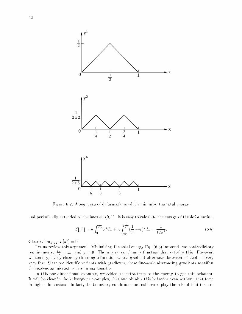
42

y

x

1

12

12

10

y

x

2

12 x 2

112

14

34

0

y

x

6

12 x 6

116

0 13

23

Figure 6.2: A sequence of deformations which minimize the total energy.

and periodically extended to the interval (0; 1). It is easy to calculate the energy of the deformation,

E [yn] = n

Z 1

2n

0x2dx+ n

Z 2

2n

1

2n

(1

n x)2dx =

1

12n2: (6.8)

Clearly, limn!1 E [yn] = 0.Let us review this argument. Minimizing the total energy Eq. (6.3) imposed two contradictory

requirements: dydx

= 1 and y = 0. There is no continuous function that satises this. However,we could get very close by choosing a function whose gradient alternates between +1 and 1 veryvery fast. Since we identify variants with gradients, these ne-scale alternating gradients manifestthemselves as microstructure in martensites.

In this one-dimensional example, we added an extra term to the energy to get this behavior.It will be clear in the subsequent examples, that one obtains this behavior even without that termin higher dimensions. In fact, the boundary conditions and coherence play the role of that term in

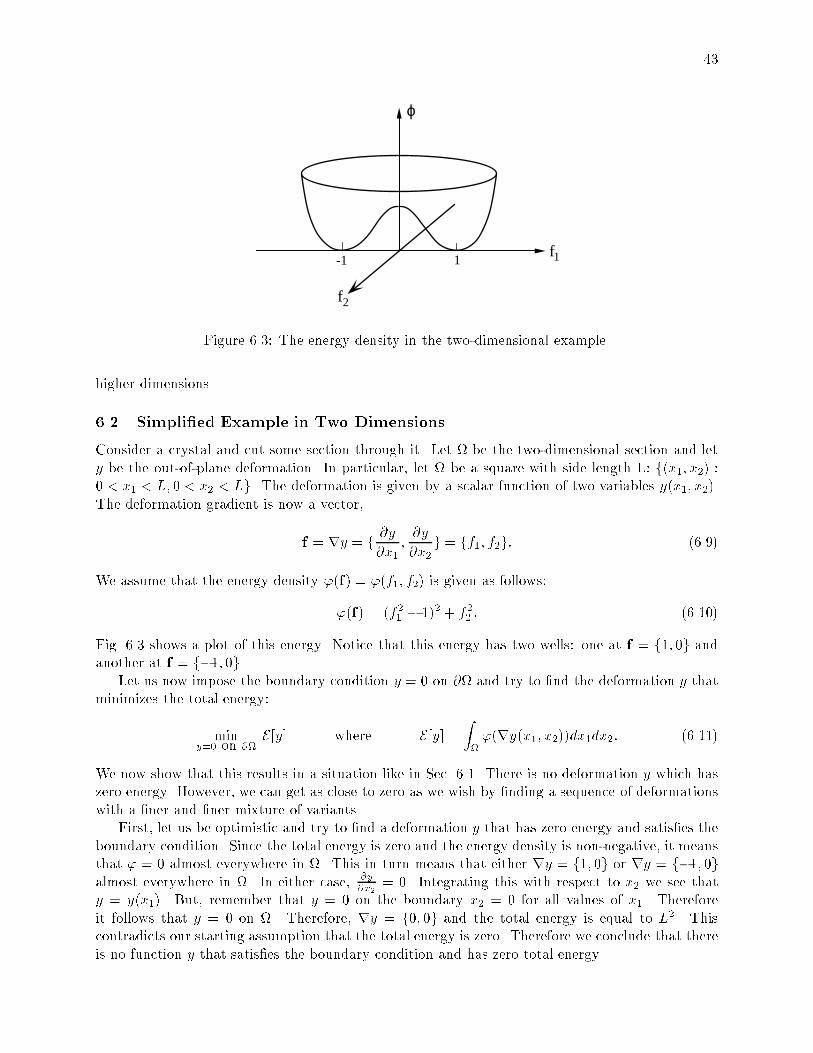
43

-1 1 1

ϕ

f

f

2

Figure 6.3: The energy density in the two-dimensional example.

higher dimensions.

6.2 Simplied Example in Two Dimensions

Consider a crystal and cut some section through it. Let be the two-dimensional section and lety be the out-of-plane deformation. In particular, let be a square with side length L: f(x1; x2) :0 < x1 < L; 0 < x2 < Lg. The deformation is given by a scalar function of two variables y(x1; x2).The deformation gradient is now a vector,

f = ry = f @y@x1

;@y

@x2g = ff1; f2g: (6.9)

We assume that the energy density '(f) = '(f1; f2) is given as follows:

'(f) = (f21 1)2 + f22 : (6.10)

Fig. 6.3 shows a plot of this energy. Notice that this energy has two wells: one at f = f1; 0g andanother at f = f1; 0g.

Let us now impose the boundary condition y = 0 on @ and try to nd the deformation y thatminimizes the total energy:

miny=0 on @

E [y] where E [y] =Z'(ry(x1; x2))dx1dx2: (6.11)

We now show that this results in a situation like in Sec. 6.1. There is no deformation y which haszero energy. However, we can get as close to zero as we wish by nding a sequence of deformationswith a ner and ner mixture of variants.

First, let us be optimistic and try to nd a deformation y that has zero energy and satises theboundary condition. Since the total energy is zero and the energy density is non-negative, it meansthat ' = 0 almost everywhere in . This in turn means that either ry = f1; 0g or ry = f1; 0galmost everywhere in . In either case, @y

@x2= 0. Integrating this with respect to x2 we see that

y = y(x1). But, remember that y = 0 on the boundary x2 = 0 for all values of x1. Thereforeit follows that y = 0 on . Therefore, ry = f0; 0g and the total energy is equal to L2. Thiscontradicts our starting assumption that the total energy is zero. Therefore we conclude that thereis no function y that satises the boundary condition and has zero total energy.

44

10

-1 0

-1 0

-1 0

10

10

12 x 3

31x2

x 1

z3

x

x1

2

(a) (b)

Figure 6.4: (a) A roof-like deformation with alternating gradients. (b) The gradients of the defor-mation shown in (a).

Second we show that there is a sequence of functions yn such that the total energy of yn goesto zero as n goes to innity. In other words, we can nd a deformation whose energy is as smallas necessary. We want to construct a deformation whose energy is small. So let us start withdeformations whose energy is zero. That means that we have to start with deformations whosegradients are either f1; 0g or f1; 0g. See the \roof-like" functions shown in Fig. 6.4. Given anyinteger n, we divide into 2n strips and construct a deformation zn where the gradient alternatesbetween rzn = f1; 0g and rzn = f1; 0g.

Each of these deformations have zero energy, but none of them satises the boundary condition.So we have to modify them. In fact, let us do so as shown in Fig. 6.5 by cutting o the roofs in atriangular region in the front and the back to obtain the deformation yn. Since the gradients in thesetriangular regions do not belong to the wells, the deformations yn do not have zero energy. However,notice something. As n becomes larger, the heights of the roofs become smaller. Therefore, theinterpolating triangles become smaller. So, let us now calculate the energy of these deformations:

E [yn] =

Ztop triangles

'(0;1)dx1dx2 +Zbottom triangles

'(0; 1)dx1dx2

+Zrest of

'(1; 0)dx1dx2

= '(0;1) (area of top triangles) (no. of top triangles) (6.12)

+ '(0; 1) (area of bottom triangles) (no. of bottom triangles)

= 2 L2

4n2 n+ 2 L2

4n2 n

=L2

n

45

10

-1 0

-1 0

-1 0

10

10

12 x 3

31

x2

x 1

01

0-1

0-1

0-1

01

01

1

1

10

-1 0

12 x 6

61

x2

x 1

0-1

10

-1 0

10

-1 0

10

-1 0

10

-1 0

10

-1 0

0-1

0-1

0-1

0-1

0-1

0 1

0 1

0 1

0 1

0 1

0 1

y 3x2

x1

y 6x2

x1

(a)

(b)

Figure 6.5: A sequence of deformations that minimize the total energy. The third and sixth elementsof this sequence are shown in (a) and (b) respectively. The deformations are shown on the left andtheir gradients are shown on the right.

46

Thus we see that the energy goes to zero as n goes to innity. In summary, when subjected tozero boundary condition, the material prefers to make a very ne mixture of the two variants in anattempt to reduce its energy.

We quickly review the argument. Energy minimization forces the gradients to take the valuesat the wells f1; 0g while the boundary condition forces the average gradient to be f0; 0g. Thematerial achieves this by making a mixture of the two wells. This causes the deformation gradientto be piecewise constant and the deformation to have a zig-zag nature. Because of the zig-zagnature of the deformation, it can not meet the boundary conditions unless they are very very ne.Therefore, the microstructure arises as the material tries to minimize the energy on the one handand tries to satisfy imposed boundary condition on the other.

The following is also clear from this example. If there were only one well, energy minimizationwould not force mixtures and therefore would not force microstructure. Thus, microstructure is adirect consequence of the multi-well nature of the energy density.

6.3 Example in Three Dimensions: Fine Twins

We now turn to an example in three dimensions which is very similar to the two-dimensionalexample above. Consider two matrices A;B which satisfy

AB = a n (6.13)

for some vectors a and n. Set

F = A+ (1 )B for some 2 (0; 1): (6.14)

Assume that we have a material whose stored energy density has the following properties:

'(A) = '(B) = 0; but '(F) > 0 for every 0 < < 1: (6.15)

Notice that we have such a situation in Fig. 5.1b if we set A = Q1UI ;B = Q2UJ .Suppose we take this material and subject it to the boundary condition y = Fx on @ for

some given . What microstructure do we expect to see? Let us rst look at the energy of thehomogeneous deformation y = Fx:

E [y] =Z'(ry)dx=

Z'(F)dx = Vol()'(F) > 0: (6.16)

Therefore, the homogeneous deformation corresponding to the boundary condition has positiveenergy. However, we will now show that we can reduce the energy to zero by making a ne-scalemixture or microstructure of A and B. In other words, we can nd a sequence of deformationsfyng such that the total energy goes to zero in the limit: limn!0 E [yn] = 0. The idea is very similarto the examples above.

Since '(A) = '(B) = 0, let us rst construct a deformation with gradients A and B. For anypositive integer n, consider the deformation zn shown in Fig. 6.6a. This deformation is continuousbecause A;B satisfy the compatibility condition Eq. (6.13). It consists of alternating layers withdeformation gradientsA and B. Therefore, the deformed shape resembles the roof-like deformationFig. 6.4 in our previous example. Clearly, E [zn] = 0. Further, the spacing between the interfacesdecreases with increasing n so that we have many many roofs and the function zn approaches thehomogeneous deformation y = Fx. In fact, it is easy to show that

jzn Fxj c

n(6.17)

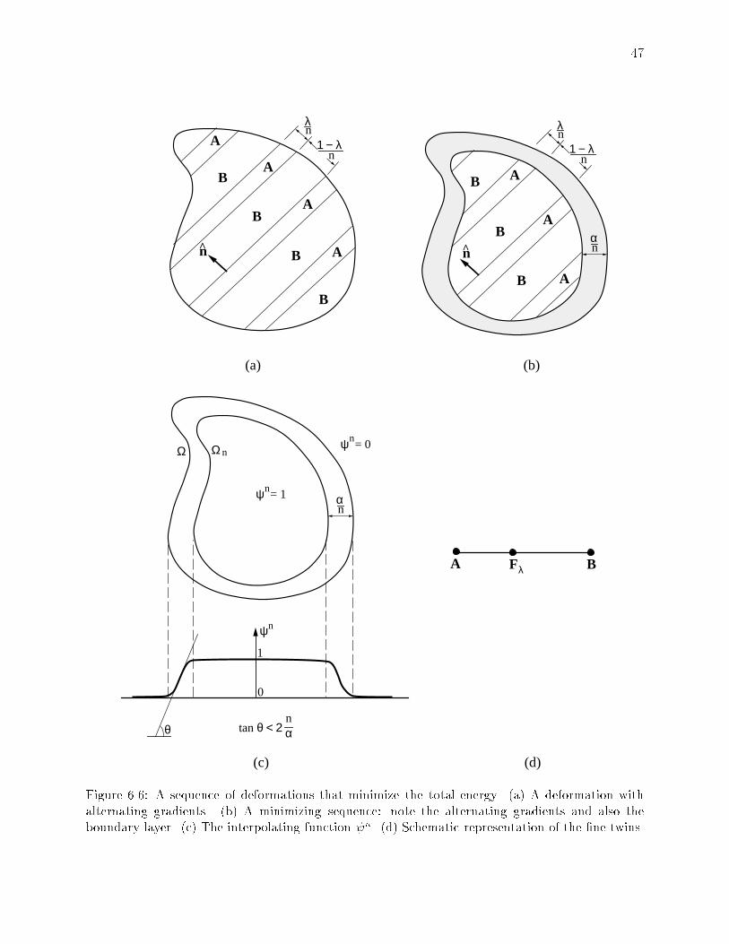
47

(c) (d)

n

A

A

A

A

B

B

B

λn

1 − λn

Ω

ψ = 1

Ω nψ = 0

αn

ψ

1

0

θ tan θ < 2αn

B

n

A

A

A

B

B

B

λn

1 − λn

αn

A F Bλ

(a) (b)

n

n

n

Figure 6.6: A sequence of deformations that minimize the total energy. (a) A deformation withalternating gradients. (b) A minimizing sequence: note the alternating gradients and also theboundary layer. (c) The interpolating function n. (d) Schematic representation of the ne twins.

48

for some constant c. Unfortunately, no matter what n we choose, we never satisfy the boundarycondition exactly; instead, it is always jagged. We x this with a boundary layer or interpolationlayer as before. This gives us a sequence of deformations yn shown in Fig. 6.6b. Since the gradientsin the interpolation layer take values other than A and B, the energy is not zero in this layer.However, as n becomes large, the volume of the interpolation layer goes to zero while the gradientsdo not blow up. Therefore, the total energy goes to zero. Thus we have a sequence which satisesthe boundary condition and whose energy goes to zero in the limit. It consists of layers of A andB alternating at a very small length-scale with a volume fraction .

Let us now discuss the construction of the interpolation layer. In the example in Sec. 6.2, wedid so by introducing the triangles and guessing the gradients. However, such a specic construc-tion becomes more and more dicult in complicated examples. Therefore we introduce a generalconstruction following Chipot and Kinderlehrer [57]. For any n, consider the region n obtainedby removing a layer of thickness

nfrom the boundary of ,

n =

x 2 : distance(x; @)>

n

: (6.18)

We wish to keep the deformation zn inside n, but change it in the annular region n sothat it satises the requisite boundary condition. We have to do so in such a manner that thegradient of the resulting deformation does not blow up as n!1. Here is a rather general way ofaccomplishing this. Consider a scalar function n shown in Fig. 6.6c with the following properties:

1: n(x) =

8><>:

0 outside

1 inside n

and 2: jr nj 2n

everywhere: (6.19)

Now setyn(x) = n(x)zn(x) + (1 n(x))Fx: (6.20)

Clearly, yn = zn inside n and it satises the boundary condition, i.e., yn = Fx on @. We justhave to check that the ryn does not blow up. Dierentiating the above,

ryn = r n zn + nrzn r n (Fx) + (1 n)F

= r n (zn Fx) + nrzn + (1 n)F:(6.21)

Therefore,jrynj jr njjzn Fxj+ j njjrznj+ j1 njjFj

2n

cn+ j njjrznj+ j1 njjFj

constant independent of n:(6.22)

Above we have used Eq. (6.19)2 and Eq. (6.17) in the rst term. In the second and the third, wehave used j nj 1, j1 nj 1 (see Eq. (6.19)1) and also rzn = A or B. Therefore,

E [yn] =Z'(ryn)dx =

Zn

'(ryn)dx CVol( n) (6.23)

which goes to zero as n goes to innity. Therefore, yn is a minimizing sequence. It consists oflayers of gradient A and B alternating at a very ne length-scale. In summary, we conclude thatwhen subjected to this boundary condition, our material makes a microstructure of A and B.

We represent this schematically as shown in Fig. 6.6d. Recall (Fig. 5.1b) that we join matriceswhich are compatible with a straight line. Therefore, we join A and B. We mark F as a point onthis line because we obtain it as a mixture of A and B. Further, the position of the point on the

49

line depends on the volume fraction according to Eq. (6.14); we are close to A if is close to 1and close to B if is close to 0. Thus, points on the straight line joining two matrices represent ane-scale mixture at the correct volume fraction.

We close with two comments. First, notice that we can not construct this sequence for any pairof matrices A and B. Instead, they must satisfy the compatibility condition Eq. (6.13). Second,it is very important that the deformation gradient does not blow up in the interpolation region.Notice in this example that the sequence of alternating gradients is compatible in some averagesense with the imposed boundary condition F as a consequence of Eq. (6.17). This allows usto construct the boundary layer which satises Eq. (6.23). If instead, we had tried to interpolatewith some other boundary condition F, the mismatch would increase with increasing n, and thegradient would go to innity. This in turn would cost innite energy even though the volume ofthe interpolation region goes to zero. Therefore, we can interpolate with diminishing energy onlybetween functions where the mismatch is decreasing with increasing n.

6.4 Weakly Converging Sequences and Microstructure

We will see more examples of sequences and microstructure in Sec. 7. Before we do so, let us collecta few of the salient features of the examples above. In each example, energy minimization led us toconstruct a sequence of deformations. Here are some of the general properties of these sequences.

1. Each deformation in the sequence is continuous.

2. The sequence of deformations converges uniformly as n goes to innity. Notice that yn ! 0in the one and two dimensional examples, while yn ! Fx in the three dimensional example.

3. The deformation gradients do not converge at any point. In the one-dimensional example, letus pick some point x and look at the gradient fn at this point. It jumps around between thevalues +1 or 1 and does not converge. Similarly, the gradient jumps around between f1; 0gand f1; 0g in the two-dimensional example, and between A and B in the three-dimensionalexample.

4. The deformation gradients converge in the average. In other words, if we pick any point andconsider any small region around it, then the average value of the deformation gradient in thisregion converges as n ! 1. Take for example, a small interval (a; b) in the one-dimensionalexample. We can divide the interval (a; b) into two regions: one where the gradient fn = 1and another where the gradient fn = 1. As n becomes large, the length of these tworegions become almost equal. Therefore the average value of the deformation gradient in thisinterval (a; b) approaches the limit 1

2(+1) +12(1) = 0. Similarly, the average value of the

deformation converges to 12f+1; 0g+ 1

2f1; 0g = f0; 0g in the two-dimensional example andto A+ (1 )B = F in the three-dimensional example.

5. The deformation gradients remain uniformly bounded. In other words, they do not becomelarger and larger as n! 1. Notice that this is true even in the triangle of the two-dimensionalexample and interpolation region in the three-dimensional example.

We call any sequence with these properties a weakly converging sequence. It is clear from theexamples above, that such sequences can be regarded as a description of the microstructure that isobserved in these materials.

Let us now try to understand the circumstances in which energy minimization forces a ma-terial to form microstructure. Let us go back to the one-dimensional example. The sequence

50

of deformations that we considered has a limit y1 = 0. The energy of this limit deformationE [y1] = R 1

0 '(ry1)dx = '(0) = 1. On the other hand, the limit of the energy limn!1 E [yn] = 0according to Eq. (6.8). Therefore, the energy of the limit is greater than the limit of the energy:

E [y1] > limn!1 E [y

n]: (6.24)

This is because the deformation gradient is equal to 0 in the limit, but has the values 1 for anyn; thus by forming a sequence we can take advantage of the fact that the fact that

'(0) > '(1) (6.25)

for our two well energy. Thus, the microstructure arises as the material takes advantage of themulti-well energy. If on the other hand, we have a material which satises

E [y1] limn!1 E [y

n] = 0 (6.26)

for each weakly converging sequence. Then, making alternating gradients does not help the ma-terial to minimize the energy. A one-well structure gives us this property which is called lowersemi-continuity of the energy. In fact, notice that we do not see any microstructure above thetransformation temperature where we have only one well the austenite well. We refer the readerto [58, 59, 60] for further discussion of these mathematical issues.

6.5 Length-Scale of the Microstructure

Let us conclude with a short discussion of what controls the length-scale of the microstructure.In the theory presented above, the microstructure is innitely ne. However, in reality, the mi-crostructure is not innitely ne, but has some distinct length-scale. So what determines the lengthscale? The answer to this is not completely clear, though we have a few guesses.

The rst and the most obvious is the interfacial or the twin-boundary energy [11, 45, 61, 62, 63].Let us go back to the two-dimensional example. Suppose that in addition to the bulk energy, we havean interfacial energy. Suppose for simplicity that this is a constant o per unit length. Thereforethe total energy bulk plus interfacial for the deformation yn is given by

Total Energy = bulk energy according to Eq. (6.12)+ o (length of each interface) (number of interfaces)

=L2

n+ o (L) (n)

=L2

n+ 2Ln o

(6.27)

Notice that this is not minimized at n = 1. As n becomes large, the bulk energy goes downbut the interfacial energy goes up. The sum is in fact minimized at n = C

pL for some constant

C. Therefore, the length-scale of the minimizing microstructure is proportional topL where L

is the length of the specimen. This is in general qualitative agreement with experiments, see forexample Arlt [62]. However, there are some deciencies. We took a minimizing sequence of thebulk energy and applied the surface energy to it. What we should do instead is to minimize thesum of the bulk and the surface energy. Kohn and Muller [63] show in an example that this leads toa microstructure which renes near the boundary, but is coarse in the interior. Once again, thereis general qualitative agreement with experiments [61].

51

m

Single Variant ofMartensiteI

QUI

Austenite

Ω

Ω2

1

Figure 7.1: An exact austenite-martensite interface.

The second factor in determining the length-scale is dynamics. While energy minimization isa good way to understand some aspects of microstructure, microstructure forms by some dynamicprocess. There is some evidence that dynamic evolutionary processes might impose some length-scale [64].

Finally, we are using a continuum theory. This is good only up to some length-scale; beyondthat, we have to use some more complete theory.

In any case, despite the failure of the theory presented above to capture the length-scale, thetheory is very successful in capturing many aspects of the microstructure as we will see in the nextsection.

7 Special Microstructures

In this section we study some important microstructures. We use two key ideas. The rst is thata microstructure can be represented using a sequence of deformations with ner and ner details.The second is that that energy minimization forces the gradients of these sequences to take valuesonly in the energy wells. Therefore, we construct sequences of deformations whose gradients belongto the energy wells. Based on these constructions, we will see that we can predict various aspectsof the microstructure.

7.1 Austenite-Martensite Interface

Perhaps the most signicant microstructure in the study of martensites is the austenite-martensiteinterface or habit plane. Therefore, let us look at this interface. Let us begin with the simplestsituation shown in Fig. 7.1 where a planar interface separates the austenite and the Ith variantof martensite. We call this an exact austenite-martensite interface. To form such an interface, weseek a continuous deformation y such that

ry =

(I in 1

QUI in 2for some rotation Q. (7.1)

If the deformation has to be continuous, we have to satisfy the compatibility or coherence condition

QUI I = b m (7.2)

for some vectors b and m. We appeal to Result 5.2 to see if this is possible. Substituting F =QUI ;G = I in step 1 of this result, we see that

C = GTFTFG1 = I(QUI)T (QUI)I = UIQ

TQUI = U2I : (7.3)

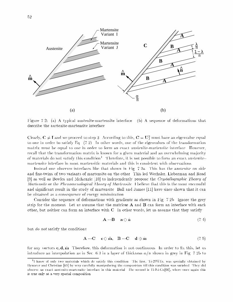
52

m

MartensiteVariant I

MartensiteVariant JAustenite

m

αn

A

A

A

B

B

B

λn

1 − λn

A

n

C

(a) (b)

Figure 7.2: (a) A typical austenite-martensite interface. (b) A sequence of deformations thatdescribe the austenite-martensite interface.

Clearly, C 6= I and we proceed to step 3. According to this, C = U2I must have an eigenvalue equal

to one in order to satisfy Eq. (7.2). In other words, one of the eigenvalues of the transformationmatrix must be equal to one in order to form an exact austenite-martensite interface. However,recall that the transformation matrix is known for a given material and an overwhelming majorityof materials do not satisfy this condition1 . Therefore, it is not possible to form an exact austenite-martensite interface in most martensitic materials and this is consistent with observations.

Instead one observes interfaces like that shown in Fig. 7.2a. This has the austenite on sideand ne-twins of two variants of martensite on the other. This led Wechsler, Lieberman and Read[9] as well as Bowles and McKenzie [10] to independently propose the Crystallographic Theory of

Martensite or the Phenomenological Theory of Martensite. I believe that this is the most successfuland signicant result in the study of martensite. Ball and James [11] have since shown that it canbe obtained as a consequence of energy minimization.

Consider the sequence of deformations with gradients as shown in Fig. 7.2b. Ignore the greystrip for the moment. Let us assume that the matrices A and B can form an interface with eachother, but neither can form an interface with C. In other words, let us assume that they satisfy

AB = a n (7.4)

but do not satisfy the conditions

AC = c m; B C = d m (7.5)

for any vectors c;d; m. Therefore, this deformation is not continuous. In order to x this, let usintroduce an interpolation as in Sec. 6.3 in a layer of thickness =n shown in grey in Fig. 7.2b to

1I know of only two materials which do satisfy this condition. The rst, Ti-29%Ta, was specially obtained byBywater and Christian [65] by very carefully manipulating the composition till this condition was satised. They didobserve an exact austenite-martensite interface in this material. The second is Ti-Ni-Cu[66], where once again thisis true only at a very special composition.

53

Q'QUJ

UJ

UI

λ Q'QU + (1- λ) Q'UIJQ'UI

I

Figure 7.3: The schematic representation of an austenite-martensite interface.

obtain a continuous deformation yn. Now, let n ! 1. Clearly, the volume of the interpolationregion goes to zero. But we want to make sure that the gradients in this region does not blow up.This is possible if and only if the average deformation on both sides are compatible, i.e., if and onlyif

(A+ (1 )B)C = b m (7.6)

for some vectors b; m. Therefore, the sequence of deformations in Fig. 7.2b is a minimizing sequenceif and only if A;B;C belong to the energy wells and

1: AB = a n2: (A+ (1 )B)C = b m:

(7.7)

Let us now see if it is possible to obtain an austenite-martensite interface as shown in Fig. 7.2aas a minimizing sequence described above. We set

C = I; B = Q2UI ; A = Q1UJ (7.8)

so that these matrices belong to the relevant energy wells. Substituting these in Eq. (7.7) andrewriting it, we obtain

1: QUJ UI = a n2: Q0(QUJ + (1 )UI) = I+ b m

(7.9)

where Q = QT2Q1 and Q0 = Q2 are rotations. These relations are shown schematically in Fig. 7.3.

Therefore, we conclude that we can form an interface between the austenite and ne twins of theIth and Jth variants of martensite if and only if we can satisfy Eq. (7.9) for some rotations Q;Q0,vectors a;b; n; m and some scalar satisfying 0 1. Notice that the rst of the equationsabove is the twinning equation. We call the second the austenite-martensite interface equation.

Before we try to solve these, let us us show that we can obtain the crystallographic theory ofmartensite from Eq. (7.9). Substituting Eq. (7.9)1 in Eq. (7.9)2, we can rewrite Eq. (7.9)2 as

I+ b m = Q0(UI + a n) = Q0(I+ a (U1I n))UI (7.10)

Recall from Sec. 5.2 that a (U1I n)) = 0 and hence, the (I + a (U1I n)) describes a simpleshear. Introducing the notation

p = b; d = m; R = Q0; S = (I+ a (U1I n)); B = UI (7.11)

54

we can rewrite the above in the traditional manner:

RSB = I+ pd: (7.12)

In other words, we obtain an invariant plane by applying a Bain distortion B, a lattice-invariantshear S and a rotation R. This is one statement of the crystallographic theory [7].

Let us now try to solve Eq. (7.9). We already know how to solve the twinning equation, Eq.(7.9)1. Let us assume that it has a solution and we have determined Q; a; n. Based on it, we cansolve the austenite-martensite interface equation using the following result of Ball and James [11].

Result 7.1 Given a matrix UI and vectors a; n which satisfy the twinning equation, Eq. (7.9)1, wecan obtain a solution to the austenite-martensite interface equation, Eq. (7.9)2, using the followingprocedure.

1. Calculate

= a UI (U2I I)1n and = tr(U2

I) det(U2I) 2 +

jaj22

: (7.13)

The austenite martensite interface equation has a solution if and only if

2 and 0: (7.14)

2. To nd the solutions, calculate

=1

2

1

r1 +

2

!: (7.15)

3. Calculate

C = (UI + n a)(UI + a n): (7.16)

Find the eigenvalues 1 2 3 and the corresponding eigenvectors e1; e2; e3 of C. Auto-matically, 2 = 1. The following solve the austenite-martensite interface equation:

b =

0@s3(1 1)3 1

e1 +

s1(3 1)

3 1 e3

1A

m =

p3

p1

p3 1

p1 1e1 +

p3 1e3

(7.17)

where is chosen to make jmj = 1 and = 1. Notice that by choosing = +1 we obtainone solution (b+; m+) while by choosing = 1 we obtain another (b; m). For eachsolution, we can obtain Q0 from Eq. (7.9)2.

4. If < 2, repeat step (3) after replacing with (1 ).Notice that for each UI ; a; n, the result above yields up to 4 solutions to Eq. (7.9)2. Further, recallthat for each pair of variants I; J , it is possible to have two solutions to the twinning equation.Therefore, for any given pair of variants, it is possible to form up to eight austenite-martensiteinterfaces.

55

7.1.1 Cubic to Tetragonal Transformation

The transformation matrices for this case are given in Table 4.1, and the possible twinning modeswere obtained in Sec. 5.4. Let us now study the austenite-martensite interfaces. Let us begin withthe variants 1 and 2. Substituting U1 according to Table 4.1 and a; n according to Eq. (5.18)1 inResult 7.1, we conclude that it is possible to form an austenite martensite interface if and only if

< 1 < and1

2+

1

2 2

or < 1 < and 2 + 2 2:

(7.18)

If equality holds, then = 12 . Otherwise,

=1

2

1

s1 +

2(2 1)(2 1)(2 + 2)

(2 2)2!: (7.19)

The two solutions with are given by

b = 1 2

1 + 2

+

2;

2;

;

m =1

+

2;

2; 1

;

where

=

s2 + 2 2

1 2 ; =

s222 2 2

1 2 ;

(7.20)

is a non-zero constant chosen to make jmj = 1. The two solutions with (1 ) are obtained byinterchanging the rst two components of b; m above. Further, if we choose the other twinningsolution Eq. (5.18)2 for this pair of variants, we would obtain four more solutions by changingthe sign of the rst component in Eq. (7.20). Thus, we obtain up to eight austenite-martensiteinterfaces for this pair of variants. Since there are three such pairs of variants, there are a total ofup to 8 3 = 24 dierent austenite-martensite interfaces in this case.

In summary, we can form an austenite-martensite interface if and only if Eq. (7.18) is satised.Then, we can have up to 24 austenite-martensite interfaces which can be obtained by permutingthe components of the vectors in Eq. (7.20).

7.1.2 Cubic to Orthorhombic transformation

The transformation matrices for this case are given in Table 4.3 and we have studied the dierenttwins in Sec. 5.5. Recall that some pairs of variants form compound twins while the other pairsform Type I and the reciprocal Type II twins.

According to Result 7.1, we can form an austenite-martensite interface using the compoundtwins if and only if

< 1; ( 1)( 1) < 0; and1

2+

1

2 2

or > 1; ( 1)( 1) < 0; and 2 + 2 2:

(7.21)

56

CB

A

AB

A

C

A

BC

m

n

D

D

n

λn

2

1 − λn

2

αn

1 − λn

1

λn

1

22

1λ A + (1- λ ) B1

2λ C + (1- λ ) D2

A

B

C

D

(a) (b)

Figure 7.4: (a) A twin within a twin. (b) Schematic representation of this microstructure.

We omit the details of the solution because common materials including CuAlNi do not satisfythese conditions. This is consistent with experimental observations.

The algebra becomes too dicult to obtain the general results for the Type I and Type IItwins. Therefore, we specialize to the case of CuAlNi. Using Result 7.1, we nd that we can forman austenite-martensite interface with either of these twins and the solutions are as follows.Interfaces using Type I twin:

= 0:2906b+ = f0:06565; 0:06573; 0:02379g; m+ = f0:6355;0:7484; 0:1897g;b = f0:05763;0:07473; 0:01700g; m = f0:7154; 0:6497; 0:2572g:

(7.22)

Interfaces using Type II twin:

= 0:3011b+ = f0:05599;0:07068; 0:02359g; m+ = f0:7306; 0:6679; 0:1420g;b = f0:06531; 0:06538; 0:01211g; m = f0:6350;0:7275; 0:2599g:

(7.23)

These solutions are for the case of for the pair of variants 1 and 3. We obtain 4 more for the case1 for this same pair of variants. Further, there are 12 pairs of variants which can form thesetwins. Therefore there are 12 (4+4) = 96 austenite-martensite interfaces. It turns out that these

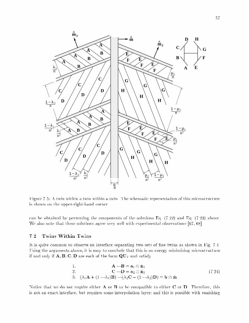
57

C

B

A

AB

A

A

m

D

αn

µn

3

2

FE

FE

FE

C

DC D H

G

H

G

H

G

B

A

A BA

A

B

C

D

C

DC D

H

G

HG

H

G

FE

FE

FE

1 − µn

3

λn

3

1 − λn

3

1 − λn

2

λn

12

21 − µ

n2µ

n22 2

λn

22

1 − λn

12

µn

12

1 − µn

12

E

m

m

1

B A

B

C

D

E

H

F

G

Figure 7.5: A twin within a twin within a twin. The schematic representation of this microstructureis shown on the upper-right-hand corner.

can be obtained by permuting the components of the solutions Eq. (7.22) and Eq. (7.23) above.We also note that these solutions agree very well with experimental observations [67, 68].

7.2 Twins Within Twins

It is quite common to observe an interface separating two sets of ne twins as shown in Fig. 7.4.Using the arguments above, it is easy to conclude that this is an energy minimizing microstructureif and only if A;B;C;D are each of the form QUI and satisfy

1: AB = a1 n12: CD = a2 n23: (1A+ (1 1)B) (2C+ (1 2)D) = b m

(7.24)

Notice that we do not require either A or B to be compatible to either C or D. Therefore, thisis not an exact interface, but requires some interpolation layer; and this is possible with vanishing

58

energy if the two sides are compatible on average, i.e., if Eq. (7.24)3 holds. It is possible to ndmany solutions to Eq. (7.24) which are consistent with observations see for example Chu andJames [69].

Let us contrast this situation with that in Sec. 5.8 where we also have four matrices. In Sec. 5.8,all four matrices meet at one point and there is no interpolation region. Therefore, notice that thecompatibility conditions Eq. (5.21) are much stricter than here Eq. (7.24). Therefore, approximateinterfaces, where only the average quantities are coherent, impose smaller restrictions.

Proceeding on similar lines, it is possible to make more and more complicated microstructure.Let us consider the twins within twins within twins as shown in Fig. 7.5. This requires that thematrices A;B;C;D;E;F;G;H are each of the form QUI and they satisfy

1: AB = a1 n12: CD = a2 n23: E F = a3 n34: GH = a4 n45: (1A+ (1 1)B) (2C+ (1 2)D) = b1 m1

6: (1E+ (1 1)F) (2G+ (1 2)H) = b2 m2

7: (3(1A+ (1 1)B) + (1 3)(2C+ (1 2)D)) (3(1E + (1 1)F) + (1 3)(2G+ (1 2)H))

= b m:(7.25)

It is important to make one comment. Notice in the Fig.7.5 that the twins (say, A and B)alternate in bands of thickness proportional to 1=n2 while the twins within twins (say, AB andCD) alternate in bands of thickness proportional to 1=n. This means that the length-scale of thetwins are much smaller than that of the twins within twins which in turn in much smaller thanthat of the macroscopic specimen. In other words, there must be a wide separation of length-scalesin order to make this successive levels of microstructure.

7.3 Wedge-like Microstructure

It is very common to observe a wedge-like or spear-like microstructure in many martensitic alloys[33, 68, 69, 70, 71, 72, 73]. When the alloy is cooled from above the transformation temperature,wedge-shaped regions of martensite grow into the austenite. As shown in Fig. 7.6, the wedgeconsists of two sets of ne twins separated by a midrib. This microstructure provides an easy wayfor the initiation of transformation and is thus important for thermoelasticity and reversibility oftransformation. It is shown in Bhattacharya [74] that only very special materials whose latticeparameters satisfy certain highly restrictive conditions can form the wedge-like microstructure.The lattice parameters of common shape-memory alloys satisfy this relation and their morphologyshows good agreement with the predictions. This suggests that microstructure and consequentlythe macroscopic behavior of martensites may depend very delicately on the lattice parameters.

Let us review the argument in [74]. The wedge-like microstructure can be represented by thesequence of deformations shown in Fig. 7.7. This minimizes the energy if and only if A;B;C;Dare each of the form QUI and they satisfy

1: AB = a1 n12: CD = a2 n23: (1A+ (1 1)B) I = b1 m1

4: (2C+ (1 2)D) I = b2 m2

5: (1A+ (1 1)B) (2C+ (1 2)D) = b m

(7.26)

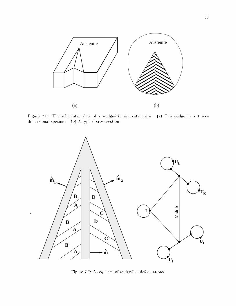
59

Austenite Austenite

(a) (b)

Figure 7.6: The schematic view of a wedge-like microstructure. (a) The wedge in a three-dimensional specimen. (b) A typical cross-section.

UJ

UI

UK

UL

Mid

rib

I

2m1m

m

A

B

C

D

AB

C

D

BA

Figure 7.7: A sequence of wedge-like deformations.

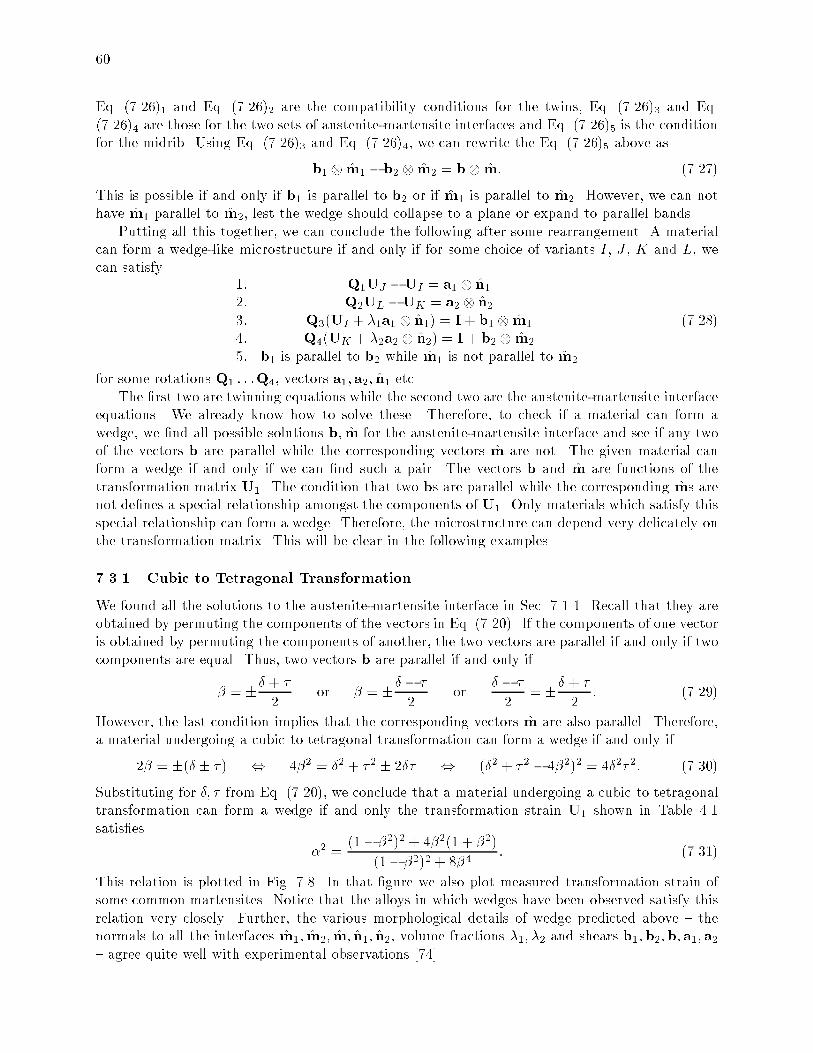
60

Eq. (7.26)1 and Eq. (7.26)2 are the compatibility conditions for the twins, Eq. (7.26)3 and Eq.(7.26)4 are those for the two sets of austenite-martensite interfaces and Eq. (7.26)5 is the conditionfor the midrib. Using Eq. (7.26)3 and Eq. (7.26)4, we can rewrite the Eq. (7.26)5 above as

b1 m1 b2 m2 = b m: (7.27)

This is possible if and only if b1 is parallel to b2 or if m1 is parallel to m2. However, we can nothave m1 parallel to m2, lest the wedge should collapse to a plane or expand to parallel bands.

Putting all this together, we can conclude the following after some rearrangement. A materialcan form a wedge-like microstructure if and only if for some choice of variants I , J , K and L, wecan satisfy

1: Q1UJ UI = a1 n12: Q2UL UK = a2 n23: Q3(UI + 1a1 n1) = I+ b1 m1

4: Q4(UK + 2a2 n2) = I+ b2 m2

5: b1 is parallel to b2 while m1 is not parallel to m2

(7.28)

for some rotations Q1 : : :Q4, vectors a1; a2; n1 etc.The rst two are twinning equations while the second two are the austenite-martensite interface

equations. We already know how to solve these. Therefore, to check if a material can form awedge, we nd all possible solutions b; m for the austenite-martensite interface and see if any twoof the vectors b are parallel while the corresponding vectors m are not. The given material canform a wedge if and only if we can nd such a pair. The vectors b and m are functions of thetransformation matrix U1. The condition that two bs are parallel while the corresponding ms arenot denes a special relationship amongst the components of U1. Only materials which satisfy thisspecial relationship can form a wedge. Therefore, the microstructure can depend very delicately onthe transformation matrix. This will be clear in the following examples.

7.3.1 Cubic to Tetragonal Transformation

We found all the solutions to the austenite-martensite interface in Sec. 7.1.1. Recall that they areobtained by permuting the components of the vectors in Eq. (7.20). If the components of one vectoris obtained by permuting the components of another, the two vectors are parallel if and only if twocomponents are equal. Thus, two vectors b are parallel if and only if

= +

2or =

2or

2= +

2: (7.29)

However, the last condition implies that the corresponding vectors m are also parallel. Therefore,a material undergoing a cubic to tetragonal transformation can form a wedge if and only if

2 = ( ) , 42 = 2 + 2 2 , (2 + 2 42)2 = 422: (7.30)

Substituting for ; from Eq. (7.20), we conclude that a material undergoing a cubic to tetragonaltransformation can form a wedge if and only the transformation strain U1 shown in Table 4.1satises

2 =(1 2)2 + 42(1 + 2)

(1 2)2 + 84: (7.31)

This relation is plotted in Fig. 7.8. In that gure we also plot measured transformation strain ofsome common martensites. Notice that the alloys in which wedges have been observed satisfy thisrelation very closely. Further, the various morphological details of wedge predicted above thenormals to all the interfaces m1; m2; m; n1; n2, volume fractions 1; 2 and shears b1;b2;b; a1; a2 agree quite well with experimental observations [74].

61

α

0.8 0.9 1.1 1.2

0.8

0.9

1.1

1.2

ab

cd

e

fg

hi

β

_ _ _ _ Wedge possible______ No volume change

(Self-accommodating)

a -- NiMnb -- NiZnCuc -- NiAld -- NiZnSie -- InTlf -- FeAlCg -- FePth -- FeCrCi -- FeNiC

Figure 7.8: The special relations that the transformation strain has to satisfy in order to form awedge, or in order to be self-accommodating. The measured lattice parameters of some alloys arealso shown. Wedges have been observed in alloys b,d,f and i while alloys a-e and g are shape-memoryalloys.

7.3.2 Cubic to Orthorhombic Transformation

Recall that a material undergoing this type of transformation can form compound, Type I andType II twins. We can form a wedge using compound twins on both sides if and only if the latticeparameters satisfy Eq. (7.21) and

2 =2a2 2

22 2+ 2 + 2 2or 2 =

2a2 2

42 2 2 2 : (7.32)

Most common materials including CuAlNi do not satisfy these conditions.The algebra gets too complicated for the Type I and Type II twins. So, the rest of the calculation

has to be carried out numerically. Bhattacharya [74] found that

We can form wedges with Type I twins on 2 surfaces in the space

We can form wedges with Type II twins on 2 surfaces in the space

CuAlNi lies extremely closely to two surfaces one with Type I twins and Type II twins [74, 75].Further, the solutions above give us various morphological details about the wedge. In particular,wedges with Type I twin resemble Fig. 7.9a while those with Type II twins resemble Fig. 7.9b. Allof these agree well with experimental observations [74].

8 Analysis of Microstructure

We understood why martensitic materials form microstructure in Sec. 6 and we studied some veryinteresting examples in Sec. 7. In the process, we developed a description of microstructure and amethod for constructing them. Using these, we can construct as many dierent examples as wish.

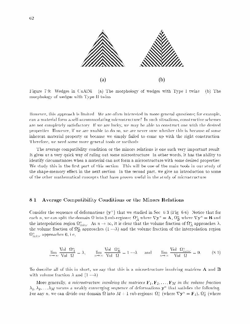
62

(a) (b)

Figure 7.9: Wedges in CuAlNi. (a) The morphology of wedges with Type I twins. (b) Themorphology of wedges with Type II twins.

However, this approach is limited. We are often interested in more general questions; for example,can a material form a self-accommodating microstructure? In such situations, constructive schemesare not completely satisfactory. If we are lucky, we may be able to construct one with the desiredproperties. However, if we are unable to do so, we are never sure whether this is because of someinherent material property or because we simply failed to come up with the right construction.Therefore, we need some more general tools or methods.

The average compatibility condition or the minors relations is one such very important result.It gives us a very quick way of ruling out some microstructure. In other words, it has the ability toidentify circumstances when a material can not form a microstructure with some desired properties.We study this in the rst part of this section. This will be one of the main tools in our study ofthe shape-memory eect in the next section. In the second part, we give an introduction to someof the other mathematical concepts that have proven useful in the study of microstructure.

8.1 Average Compatibility Conditions or the Minors Relations

Consider the sequence of deformations fyng that we studied in Sec. 6.3 (Fig. 6.6). Notice that foreach n, we can split the domain into 3 sub-regions: n

A where ryn = A, nB where ryn = B and

the interpolation region ninter . As n!1, it is clear that the volume fraction of n

A approaches ,the volume fraction of n

B approaches (1 ) and the volume fraction of the interpolation regionninter approaches 0, i.e,

limn!1

Vol. nA

Vol. = ; lim

n!1Vol. n

B

Vol. = 1 and lim

n!1Vol. n

inter

Vol. = 0: (8.1)

To describe all of this in short, we say that this is a microstructure involving matrices A and Bwith volume fraction and (1 ).

More generally, a microstructure involving the matrices F1;F2; : : : ;FM in the volume fraction

1; 2; : : :M means a weakly converging sequence of deformations yn that satises the following.For any n, we can divide our domain into M + 1 sub-regions: n

1 (where ryn = F1), n2 (where

63

ryn = F2), . . . , nM (where ryn = FM) and an interpolation region n

inter . Further,

limn!1

Vol. n1

Vol. = 1; lim

n!1Vol. n

2

Vol. = 2; : : : lim

n!1Vol. n

M

Vol. = M ;

limn!1

Vol. ninter

Vol. = 0;

where m 0; andMXm=1

m = 1:

(8.2)

We use this terminology to state a very important result.

Result 8.1. Average compatibility conditions or the minors relations. Morrey [76]Suppose we have a microstructure involving the matrices F1;F2; : : : ;FM in the volume fraction1; 2; : : :M . Suppose further that the microstructure satises the boundary condition corre-sponding to the matrix F; i.e., yn = Fx on the boundary @. Then, the following are true.

1: F =MX

m=1

mFm

2: cof F =MXm=1

m(cof Fm)

3: detF =MXm=1

m(detFm)

(8.3)

Further, if detF1 = detF2 = : : := detFM 6= 0, then we can rewrite the second relation above, Eq.(8.3)2 as

FT =MX

m=1

mFTm : (8.4)

We will soon see that these relations have the following interpretation. The rst relation, Eq.(8.3)1, says in some average way that lines remain unbroken in a coherent microstructure, thesecond relation, Eq. (8.3)2, says that planes or surfaces remain unbroken and the third relation,Eq. (8.3)3, says that volumes remain unbroken. Therefore, we call these the average compatibilitycondition.

We will use these extensively in the next section. Notice that these relations impose very severerestrictions on the matrices that can participate in a microstructure. Suppose we have some matricesF1;F2; : : : ;FM for which we can not satisfy these relations for any volume fractions m, then wecan immediately say that we can not construct a microstructure with these matrices. The rst ofthese relations is widely known and used even in the materials science literature (see for exampleSaburi and Wayman [77]). The other two are relatively unknown in this literature, but have playeda very central role in the recent mathematical treatments see for example, [21, 50, 78, 79]. Infact, these relations in one form or the other have been very used in a variety of subjects includingnonlinear elasticity and composite materials (see for example, [58, 76, 80, 81, 82]).

We now turn to understanding and proving these conditions. We begin with a simple argumentin a special case. This gives us the physical interpretation. We take the reference crystal to

64

F

x

2 3FF

x x x

1

0 2 k1

y(x )01y(x )

y(x )ky

Figure 8.1: A continuous piece-wise homogeneous deformation that satises homogeneous boundaryconditions. Notice that a straight line in the reference conguration becomes jagged but remainsunbroken after deformation.

be an unit cube see Fig. 8.1. Let us ignore the interpolation region; so we have a continuousdeformation y which satises the boundary condition y = Fx on @ and whose gradients take thevalues F1;F2; : : : ;FM with volume fraction 1; 2; : : :M . We choose our coordinate system to beparallel to the edges of the cube.

We begin with the rst relation, Eq. (8.3)1. Consider any point xo = f0; x2; x3g on the left faceof the reference cube and consider a line parallel to the x1 axis that passes through it. Let us marksome K points x1;x2; : : : ;xK on the reference line in such a manner that any segment (xk1;xk)lies completely in a region with constant gradient. After deformation, this straight line goes to ajagged, but unbroken, line as shown in Fig. 8.1. Since the line remains unbroken after deformation,we can obtain the vector joining the end points by simply taking the vector sum of the dierentsegments:

y(xK) y(xo) =KXk=1

(y(xk) y(xk1)) : (8.5)

This is the key idea behind Eq. (8.3)1. The rest is just a matter of calculation to express this interms of the gradients. First, notice that both xo and xK are on the boundary @; so we can usethe boundary condition to calculate

y(xK) y(xo) = FxK Fxo = F(xK xo) = Fe1 (8.6)

where e1 is the unit vector parallel to the x1 axis. Second, the gradient is constant in the linesegment (xk1;xk),

y(xk) y(xk1) = Fk(xk xk1) = Fk(ke1) = kFke1: (8.7)

Above, we have used the fact that (xkxk1) is parallel to e1 and has length k. Substituting Eq.(8.6) and Eq. (8.7) in Eq. (8.5), we obtain

Fe1 =KXk=1

(kFk e1) =

KXk=1

kFk

!e1: (8.8)

65

This relation is in fact true for any line parallel to the x1 axis though the number of segments Kand their lengths k may depend on the coordinates (x2; x3) of the starting point xo. If we averagethis relation over all such lines, i.e., if we integrate this relation over all x2; x3, we obtain,

Fe1 =

Z 1

0

Z 1

0

KXk=1

kFk

!e1dx2dx3 =

Z 1

0

Z 1

0

KXk=1

kFkdx2dx3

!e1 =

MX

m=1

mFm

!e1 (8.9)

where m are the volume fractions of the dierent gradients. Above, we have used the fact thatintegrating the length fractions over an area gives us the volume fractions. We can similarly obtainthe relations,

Fe2 =

MX

m=1

mFm

!e2 and Fe3 =

MXm=1

mFm

!e3 (8.10)

using lines parallel to the x2 and the x3 axes. Since fe1; e2; e3g is a basis, these three relations givethe required result, Eq. (8.3)1. Once again, the key idea is that lines remain unbroken as expressedby Eq. (8.5).

Let us now turn to the second relation, Eq. (8.3)2. Consider the plane P = fx1 = constantg inthe reference conguration. We can now split this plane into K pieces, P1;P2; : : :Pk : : :PK , suchthat the gradient is constant in each of these pieces. Let k be the area fraction of the piece Pk.After deformation, this plane transforms to a \hilly landscape". Since the deformation gradientis constant in each piece Pk, these pieces remain planar even after deformation though their areaand their orientation may have changed. Since the deformation is continuous, there are no tears inthe landscape. Therefore, the area enclosed by the boundary of the plane P is given by the vectorsum of the the areas of the sub-regions Pk. This is the key idea. The rest is calculation. Recallthat from Sec. 2 that areas transform as the cof ry. Therefore, the area enclosed by the boundaryof P after deformation is given by (cof F)e1 using the boundary condition while the area of thesub-regions Pk is given by k(cof Fk)e1. Therefore, we obtain,

(cof F)e1 =

KXk=1

kcof Fk

!e1 (8.11)

where k are the area fractions. Averaging this relation over all parallel planes, i.e., integratingthis relation over all x1, we obtain

cof Fe1 =

MXm=1

mcof Fm

!e1: (8.12)

Above, we have used the fact that integrating the area fractions over a length gives us the volumefractions. We can obtain similar relations for e2 and e3, and therefore we obtain Eq. (8.3)2. Onceagain, the key idea is that planes remain unbroken after continuous deformation.

The third relation, Eq. (8.3)3 is even simpler. Recall from Sec. 2 that volume changes asthe determinant of the deformation gradient. Therefore, the volume of any subregion m afterdeformation is given by

Vol. y(m) = (detFm)(Vol. m): (8.13)

However, the boundary of the body deforms according to the boundary condition. Therefore, wecan calculate the total volume of the body after deformation as

Vol. y() = (detF)(Vol. ): (8.14)

66

Since the deformation of the body is continuous, the volume of the body is equal to the sum of thevolume of the parts:

(detF)(Vol. ) =MXm=1

(Vol. m)(detFm): (8.15)

Dividing this equation by (Vol. ) and using the denition of volume fraction, we obtain therequired relation, Eq. (8.3)3. Thus, this relation tells us that the volume of the body is equal tothe sum of the volume of the parts.

We now turn to a more general proof which uses the divergence theorem. We consider anygeneral domain and any microstructure involving the matrices F1;F2; : : : ;FM in the volumefraction 1; 2; : : :M described by a sequence, possibly with interpolation regions.

We begin with Eq. (8.3)1. For any n, consider the integral of ryn over . We can evaluate thisin two ways. The rst uses the knowledge of the values of ryn:

Zryn(x)dV =

MXm=1

Znm

ryn(x)dV +Zninter

ryn(x)dV

=MX

m=1

Znm

FmdV +

Zninter

ryn(x)dV (8.16)

=MX

m=1

(Vol. nm)Fm +

Zninter

ryn(x)dV

since we know that ryn = Fm in nm. The second uses the divergence theorem and the boundary

data. Zryn(x)dV =

Z@yn ndA

=

Z@Fx ndA

=

Zr(Fx)dV (8.17)

=

ZFdV = (Vol. )F:

We have used the divergence theorem in the rst line, the boundary condition yn = Fx on @ togo from the rst to the second line, the divergence theorem once again to go from the second tothe third and the fact that r(Fx) = F where F is a constant matrix to go from the third to thefourth. Comparing these two equations and dividing them by (Vol. ), we obtain,

F =MX

m=1

Vol. nm

Vol. Fm +

1

Vol.

Zninter

ryn(x)dV: (8.18)

Take the limit as n ! 1. Notice that the last term drops out (the volume of the interpolationregion goes to zero while the integrand remains uniformly bounded) and this equation reduces toEq. (8.3)1 using the volume fractions dened in Eq. (8.2).

Let us skip the second relation momentarily and look at the third, Eq. (8.3)3. We use thefact that the determinant is a \null-lagrangean", i.e., the integral of the determinant of a gradient

67

depends only on the boundary values. This is because we can express the determinant of a gradientas the divergence of some vector-valued function: for each y, we can nd a function fy such that

detry = r fy : (8.19)

(Here, we use the superscript y to remind us that this function is associated with the deformationy.) We will show this in a moment. We use this and the divergence theorem twice (as in Eq. (8.17))to obtainZ

detryndV =

Zr fyndV =

Z@fy

n ndA =

Z@fFx ndA

=Zr fFxdV =

ZdetFdV = (detF)(Vol. ):

(8.20)

On the other hand, we can use the knowledge of the gradients as in Eq. (8.16) to calculate

ZdetrydV =

MXm=1

(detFm)(Vol. nm) +

Zninter

detrydV: (8.21)

Comparing Eq. (8.20) and Eq. (8.21), we obtain

(Vol. )(detF) =MXm=1

(Vol. nm)(detFm) +

Zninter

detrydV: (8.22)

Dividing this relation by (Vol. ) and taking the limit as n!1, we obtain Eq. (8.3)3 as desired.We now return to Eq. (8.19). Let us introduce the permutation symbol ijk . For i; j; k = 1; 2; 3,

ijk =

8>>>>><>>>>>:

0 if i = j or j = k or i = k

+1 if i; j; k is an even permutation of 1; 2; 3, e.g. if ijk = 231

1 if i; j; k is an odd permutation of 1; 2; 3, e.g. if ijk = 213

: (8.23)

Using this symbol and the summation convention, we have a very simple formula for the determinantof any matrix A:

detA = ijkA1iA2jA3k : (8.24)

This is very easily veried, for example, by simply expanding it. Therefore,

detry = ijk@y1@xi

@y2@xj

@y3@xk

: (8.25)

Let us hold this for a moment. Notice that

@

@xi

ijky1

@y2@xj

@y3@xk

!= ijk

@y1@xi

@y2@xj

@y3@xk

+ ijky1@2y2@xi@xj

@y3@xk

+ ijky1@y2@xj

@2y3@xi@xk

: (8.26)

We claim that the last two terms are zero. Let us consider the second term. Notice that inter-changing the i and j changes the sign of ijk but leaves @2y2

@xi@xjunchanged (because of the equality

of second derivatives). Therefore, when we sum over all i and j this term reduces to zero. To see

68

this, consider the k = 3 term: summing over all i and j and writing only the non-zero terms, weobtain

ij3y1@2y2@xi@xj

@y3@x3

= 123y1@2y2@x1@x2

@y3@x3

+ 213y1@2y2@x2@x1

@y3@x3

= 123y1@2y2@x1@x2

@y3@x3

123y1@2y2@x1@x2

@y3@x3

= 0:

(8.27)

The terms for k = 1; 2 are similarly zero, and therefore the second term in Eq. (8.26) is zero. Weuse a similar argument for the third term. Therefore, comparing Eq. (8.26) and Eq. (8.25), we seethat

detry =@

@xi

ijky1

@y2@xj

@y3@xk

!: (8.28)

This is exactly the same as Eq. (8.19) if we dene the vector-valued function fy using its componentsfyi :

fyi = ijky1@y2@xj

@y3@xk

i = 1; 2; 3: (8.29)

Let us now turn to the remaining condition, Eq. (8.3)2. Using the permutation symbol ijk , thesummation convention and the formula for the cofactor of a matrix, we have

(cof ry)ij = 1

2ikljpr

@yk@xp

@yl@xr

: (8.30)

Therefore, it is possible to verify as before that

(cof ry)ij = @

@xp

1

2ikljpryk

@yl@xr

(8.31)

so that the cofactor of the gradient is the divergence of some third-order tensor eld. Thereforeusing the divergence theorem, we can conclude that the cofactor of the deformation gradient is anull-lagrangean and its integral depends only on the boundary values:Z

cof ryndV =

Zcof FdV = (cof F)(Vol. ): (8.32)

On the other hand, we can evaluate this integral using the knowledge of the gradients as in Eq.(8.16) Z

cof ryndV =

MXm=1

(cof Fm)(Vol. nm) +

Zninter

cof rydV: (8.33)

Comparing these two, we obtain

(Vol. )(cof F) =MX

m=1

(Vol. nm)(cof Fm) +

Zninter

cof rydV: (8.34)

Dividing this relation by (Vol. ) and taking the limit as n!1, we obtain the desired result, Eq.(8.3)2.

69

Finally, let us look at Eq. (8.4). By assumption, detF1 = detF2 = : : : = detFM 6= 0. We usethis in Eq. (8.3)3 to conclude that detF = detF1 6= 0. Therefore, we can use the formula for thecofactor in Eq. (2.11) to rewrite Eq. (8.3)2 as

(detF)FT =MXm=1

m(detFm)F

Tm

= (detF1)

MXm=1

mFTm : (8.35)

However, detF = detF1 and we obtain Eq. (8.4).

8.2 Young Measure and Generalizations

In the previous section, we looked at a very important result in the case of microstructures thatsatisfy homogeneous boundary condition. However, not all microstructures satisfy such boundaryconditions see for example the austenite-martensite interface or the wedge-like microstructure.Therefore, let us study some properties of some more general microstructures.

Consider any weakly convergent sequence of deformations fyng. It has the ve properties listedin Sec. 6.4. In particular, the gradients converge in some average sense. In fact, if we look in a smallregion around any point, we nd a very denite statistical distribution of the gradients as n! 1[83]. For example, consider the ne twins we studied in Sec. 6.3. If we pick any point and look ata small region near it, we nd that we have a probability of nding A and a probability (1 )of nding B as n becomes large. Or consider for example, the wedge-like microstructure shown inFig. 7.8. Here, the distribution of the gradients depend on the point that we pick. If we pick thepoint outside the wedge, we have a probability 1 of nding the gradient I; if we pick the point inthe left side of the wedge, we have a probability 1 of nding the gradient A and (11) of ndingthe gradient B; and if we pick the point on the right side of the wedge, we have a probability 2 ofnding the gradient C and a probability of (1 2) of nding the gradient D.

TheYoung measure x is the probability measure that describes this distribution of gradients in asmall region around the point x [83, 84, 85]. It is very important to emphasize one point. The Youngmeasure describes only those distributions that can be obtained from a weakly converging sequence.For example, in the ne twins in Sec. 6.3, if A;B do not satisfy the compatibility condition, thatsequence would not be weakly converging, and we would not obtain a Young measure with A andB. Therefore, the Young measure has buried within itself all information concerning compatibilityor coherence. Therefore, it is a very convenient and useful accounting device.

We can describe the dierence between classical deformations and microstructure as follows.In a classical deformation, we have only one matrix as the value of the gradient at any point.In contrast, the value of the gradient is not a single matrix in a microstructure; instead it is aprobability distribution. Further, in a coherent microstructure, this probability distribution isdescribed by a Young measure.

We conclude with a generalization of the average compatibility conditions or minors relations.Consider some weakly convergent sequence fyng whose limiting deformation is y. Suppose theYoung measure at the point x consists ofM matrices F1;F2; : : : ;FM with probability 1; 2; : : : ; M

70

a

bc

Cool Heat

deform

Temperature

Figure 9.1: The shape-memory eect.

respectively. Then,

1: ry(x) =MX

m=1

mFm

2: cof ry(x) =MXm=1

m(cof Fm)

3: detry(x) =MX

m=1

m(detFm):

(8.36)

Thus, these average compatibility conditions hold not only for the entire body, but in every smallregion of the body.

9 The Shape-Memory Eect

Shape-memory behavior is the ability of certain materials to recover, on heating, apparently plasticdeformation sustained below a critical temperature. Below the critical temperature, the alloy isextremely malleable - undergoing apparently plastic deformations with strains as large as 10%under very small forces. It is therefore possible to easily deform a piece of shape-memory materialinto a variety of new shapes. However, all the strain is recovered when it is heated to above thecritical temperature. Cooling from above to below the critical temperature does not cause anymacroscopic shape change and the cycle can be repeated. This is shown schematically in Fig. 9.1.Intensive experimental and crystallographic investigation during the 1960s and the 70s revealedthat the heart of the eect lies in the reversible or \thermoelastic" martensitic transformationthat these crystalline solids undergo. The critical temperature of the shape-memory eect is thetransformation temperature.

Consider a single crystal specimen of a given shape in Fig. 9.1a. It is in the austenite phase. Oncooling, the austenite transforms to the martensite. However, the variants of martensite arrangethemselves in such a manner that there is no macroscopic change in shape (Fig. 9.1b). This isknown as self-accommodation. When loads are applied to the martensite, it deforms by convertingone variant to another and forming a new microstructure (Fig. 9.1c). Consequently, the resultingdeformation appears macroscopically plastic: there is no restoring force since all the variants areenergetically equivalent. But in fact, this deformation is recoverable: heating the specimen abovethe transformation temperature turns each variant of martensite back to the unique variant ofaustenite and the specimen springs back to its original shape.

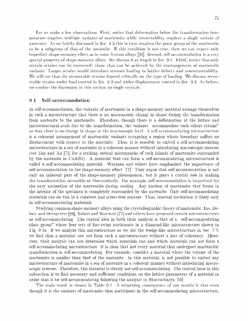
71

Let us make a few observations. First, notice that deformation below the transformation tem-perature requires multiple variants of martensite while recoverability requires a single variant ofaustenite. As we brie y discussed in Sec. 4.3 this in turn requires the point group of the martensiteto be a subgroup of that of the austenite. If this condition is not true, then we can expect onlyimperfect shape-memory eect as in some ferrous alloys [38]. Second, self-accommodation is a veryspecial property of shape-memory alloys. We discuss it at length in Sec. 9.1. Third, notice that onlycertain strains can be recovered: those that can be achieved by the rearrangement of martensitevariants. Larger strains would introduce stresses leading to lattice defects and nonrecoverability.We will see that the recoverable strains depend critically on the type of loading. We discuss recov-erable strains under load control in Sec. 9.2 and under displacement control in Sec. 9.3. As before,we conne the discussion in this section to single crystals.

9.1 Self-accommodation

In self-accommodation, the variants of martensite in a shape-memory material arrange themselvesin such a microstructure that there is no macroscopic change in shape during the transformationfrom austenite to the martensite. Therefore, though there is a deformation at the lattice andmicrostructural scale due to the transformation, the variants \accommodate each others strains"so that there is no change in shape at the macroscopic level. A self-accommodating microstructureis a coherent arrangement of martensitic variants occupying a region whose boundary suers nodisplacement with respect to the austenite. Thus, it is possible to embed a self-accommodatingmicrostructure in a sea of austenite in a coherent manner without introducing macroscopic stresses(see Tan and Xu [71] for a striking optical micrographs of such islands of martensite surroundedby the austenite in CuAlNi). A material that can form a self-accommodating microstructure iscalled a self-accommodating material. Wayman and others have emphasized the importance ofself-accommodation to the shape-memory eect [77]. They argue that self-accommodation is notonly an inherent part of the shape-memory phenomenon, but it plays a crucial role in makingthe transformation reversible or thermoelastic. For example, self-accommodation is important forthe easy nucleation of the martensite during cooling. Any nucleus of martensite that forms inthe interior of the specimen is completely surrounded by the austenite. Only self-accommodatingmaterials can do this in a coherent and stress-free manner. Thus, internal nucleation is likely onlyin self-accommodating materials.

Studying common shape-memory alloys using the crystallographic theory of martensite, Tas, De-laey and Deruyterre [86], Saburi and Wayman [77] and others have proposed certain microstructuresas self-accommodating. The central idea in both their analysis is that of a \self-accommodatingplate group" where four sets of ne-twins participate in a diamond-like microstructure shown inFig. 9.2a. If we analyze this microstructure as we did the wedge-like microstructure in Sec. 7.3,we nd that a material can not form such a microstructure without a loss of coherence. More-over, their analysis can not determine which materials can and which materials can not form aself-accommodating microstructure. It is clear that not every material that undergoes martensitictransformation is self-accommodating. For example, consider a material where the volume of themartensite is smaller than that of the austenite. In this material, is not possible to embed anymicrostructure of martensite in a sea of austenite in a coherent manner without introducing macro-scopic stresses. Therefore, this material is clearly not self-accommodating. The central issue in thissubsection is to nd necessary and sucient conditions on the lattice parameters of a material inorder that it be self-accommodating following the analysis in Bhattacharya [50].

The main result is shown in Table 9.1. A surprising consequence of our results is that eventhough it is the variants of martensite that participate in the self-accommodating microstructure,

72

Mismatchhere

2U1U

4U 3U

I

(a) (b)

Figure 9.2: Self-accommodating microstructures. (a) The commonly discussed diamond microstruc-ture. Unfortunately, this is not coherent. (b) Schematic representation of the microstructure con-structed to prove the result in Table 9.1.

the conditions for self-accommodation depend only on the symmetry of the austenite. As ex-plained above, volume preservation during transformation is necessary for self-accommodation. Itturns out that volume preservation during transformation is also sucient for self-accommodationif the symmetry of the austenite is cubic. In fact, in the case of cubic austenite, it is always possibleto construct a microstructure which is a pure dilatation with respect to the austenite. The amountof dilatation, of course, depends on the transformation volume change. However, if the symmetryof the austenite is not cubic, the lattice parameters of the material have to satisfy additional re-strictions which are extremely stringent and \non-generic". For example consider the tetragonal toorthorhombic transformation. Self-accommodation requires that dened in Table 4.2 be exactlyequal to one (i.e., there is no stretch along the \c-axis" of the tetragonal lattice during the trans-formation) in addition to the condition of no volume change during transformation. In summary,materials with cubic austenite have to satisfy a rather easy constraint while materials with non-cubic austenite have to satisfy very restrictive conditions in order to be self-accommodating. Thismay be the reason why every shape-memory material that I have found in the literature has cubicaustenite and undergoes very small volume change during transformation. In particular consideralloys that undergo the cubic to tetragonal transformation. The transformation is volume preserv-ing if and only the parameters ; dened in Table 4.1 satisfy the relation 2 = 1. This relationis plotted in Fig. 7.8, along with the measured lattice parameters of some shape-memory alloys.See [50] for more comparison with experimental observations. We now examine the proof of thisresult for a couple of cases.

9.1.1 Cubic Austenite

Any material with a cubic austenite can form a self-accommodating microstructure if and only ifdetU1 = 1 according to Table 9.1. We brie y sketch a proof of this result.

First consider a material that can form a self-accommodating microstructure. Suppose thismicrostructure involves the matrices F1;F2; : : : ;FM in the volume fraction 1; 2; : : :M . Sincethis is a microstructure of martensite, each of the matrices F1;F2; : : : ;FM belongs to the martensitewells M and consequently is of the form QUI . Therefore, for each m,

detFm = det(QUI) = (detQ)(detUI) = detUI = detU1: (9.1)

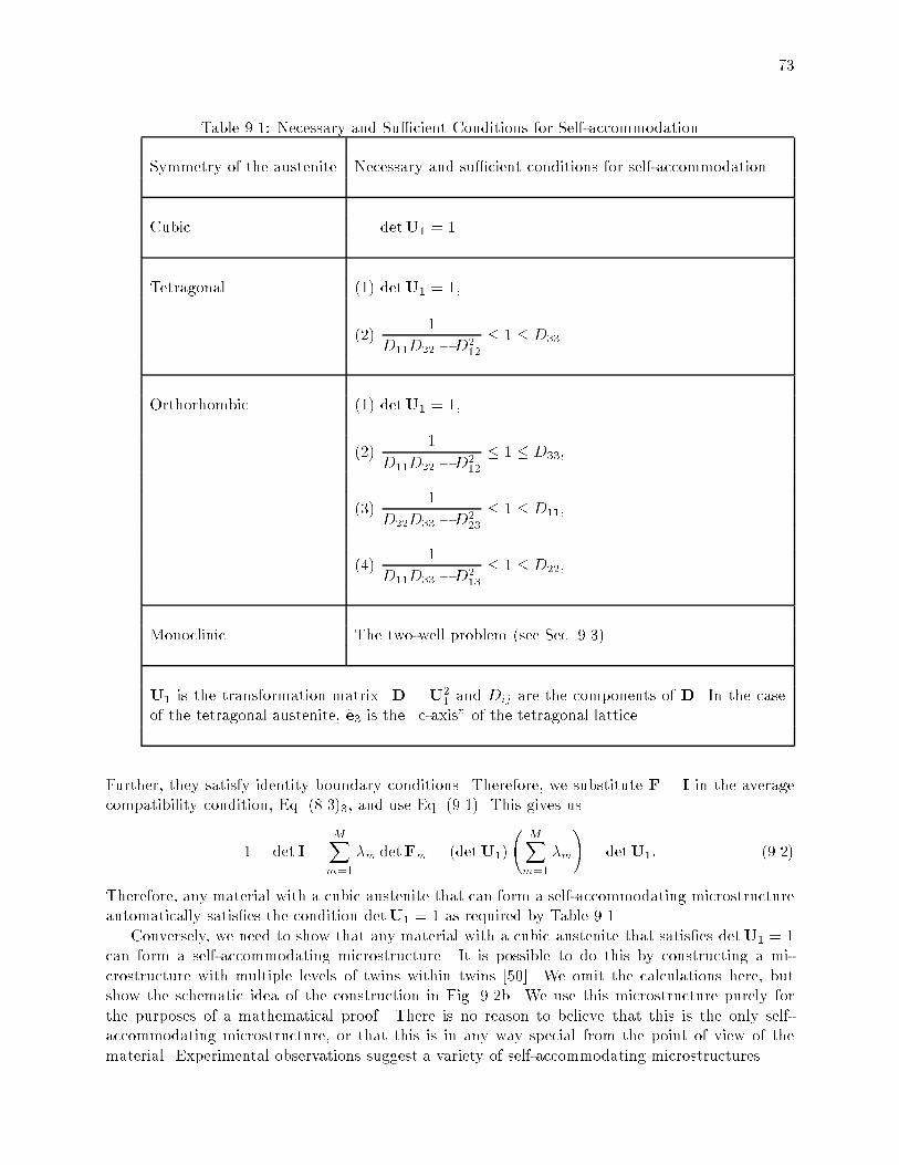
73

Table 9.1: Necessary and Sucient Conditions for Self-accommodation

Symmetry of the austenite Necessary and sucient conditions for self-accommodation

Cubic detU1 = 1

Tetragonal (1) detU1 = 1,

(2)1

D11D22 D212

1 D33

Orthorhombic (1) detU1 = 1,

(2)1

D11D22 D212

1 D33,

(3)1

D22D33 D223

1 D11,

(4)1

D11D33 D213

1 D22,

Monoclinic The two-well problem (see Sec. 9.3)

U1 is the transformation matrix. D = U21 and Dij are the components of D. In the case

of the tetragonal austenite, e3 is the \c-axis" of the tetragonal lattice.

Further, they satisfy identity boundary conditions. Therefore, we substitute F = I in the averagecompatibility condition, Eq. (8.3)3, and use Eq. (9.1). This gives us

1 = det I =MX

m=1

m detFm = (detU1)

MXm=1

m

!= detU1: (9.2)

Therefore, any material with a cubic austenite that can form a self-accommodating microstructureautomatically satises the condition detU1 = 1 as required by Table 9.1.

Conversely, we need to show that any material with a cubic austenite that satises detU1 = 1can form a self-accommodating microstructure. It is possible to do this by constructing a mi-crostructure with multiple levels of twins within twins [50]. We omit the calculations here, butshow the schematic idea of the construction in Fig. 9.2b. We use this microstructure purely forthe purposes of a mathematical proof. There is no reason to believe that this is the only self-accommodating microstructure, or that this is in any way special from the point of view of thematerial. Experimental observations suggest a variety of self-accommodating microstructures.

74

9.1.2 Tetragonal Austenite

Consider a material with tetragonal austenite. Let e3 be the axis of 4-fold symmetry or the \c-axis" of the tetragonal austenite lattice. Therefore, for each rotation R in the point group of theaustenite Pa,

Re3 = e3: (9.3)

According to Table 9.1, this material can form a self-accommodating microstructure if and only if

detU1 = 1 and1

D11D22 D212

1 D33: (9.4)

Above, we use the notation D = U21 and Dij are the components of D.

We now show that if a material is self-accommodating, then Eq. (9.4) holds. The rst part,detU1 = 1, follows from the average compatibility condition, Eq. (8.3)3, as in the cubic case. There-fore, we conne ourselves to the inequalities in Eq. (9.4)2. Let the self-accommodating microstruc-ture involve the matrices F1;F2; : : : ;FM in the volume fraction 1; 2; : : :M . Since we are lookingfor a self-accommodating microstructure of martensite, each of the matrices F1;F2; : : : ;FM be-longs to the martensite wellsM and consequently is of the form QUI . Further, this microstructuresatises identity boundary condition. Therefore, we can write the average compatibility condition,Eq. (8.3)1, as

I =MX

m=1

mFm; and hence e3 =MXm=1

mFme3: (9.5)

Therefore,

1 = je3j2 =

MXm=1

mFme3

!

MXm=1

mFme3

!: (9.6)

Now notice that the following inequality is true for any vectors a1; a2; : : :aM ,MXm=1

mam

2

=

MX

m=1

mam

!

MXm=1

mam

!

MXm=1

mjamj2: (9.7)

Therefore,

1 MX

m=1

mjFme3j2: (9.8)

However, for any m,

jFme3j2 = e3 (FTmFme3) = e3 (U2

I e3) = e3 (RTU21Re3) = (Re3) (U2

1Re3) = D33: (9.9)

Above we have used the fact that UI = RTU1R for some R 2 Pa and Eq. (9.3). Substituting thisin Eq. (9.8), we obtain

1 MXm=1

mD33 = D33 (9.10)

which is the right side of Eq. (9.4)2. We prove the other part of Eq. (9.4)2 using a very similarargument. First notice that detFm = detU1, so we can use Eq. (8.4). Since we satisfy identityboundary conditions,

I = IT =MXm=1

mFTm ; so that e3 =

MXm=1

mFTm e3 and 1

MXm=1

me3 (F1m FTm e3):

(9.11)

75

However,e3 (F1m FTm e3) = e3 (U2I e3) = e3 (U21 e3) = (D1)33: (9.12)

But,

(D1)33 =1

detD(D11D22 D2

12) =D11D22 D2

12

(detU1)2= D11D22 D2

12: (9.13)

Putting these together,

1 D11D22 D212 or

1

D11D22 D212

1 (9.14)

which is the left half of the inequality in Eq. (9.4)2. Thus, we conclude that any self-accommodatingmaterial with a tetragonal austenite satises Eq. (9.4). The converse of the result can once againbe demonstrated using a construction shown schematically in Fig. 9.2b [50].

9.2 Recoverable Strains under Load Control

Consider a single crystal that has just been transformed from the austenite to the martensite (Fig.9.1b). Therefore, it is at a temperature below the transformation temperature and is in the self-accommodated state. We are interested in nding the maximum deformation that the single crystalcan undergo by rearranging its variants. We will see that this depends critically on the type of load load control or displacement control and on the orientation.

In this section we assume the crystal is deformed under load control (or dead loads). In otherwords, we assume that t, the applied force per unit reference area on the boundary of the body, isheld constant as the specimen deforms. Let us further assume that the applied load corresponds toa constant matrix S: i.e., t = Sn where n is the unit outward normal in the reference conguration.We claim following James [87] that the state of crystal subjected to this load is described by thedeformation y that minimizes the energyZ

('(ry) S ry)dV: (9.15)

We can interpret the integrand as a generalization of the Gibbs free energy for multiaxial loading.Notice that the integrand depends only on ry and does not explicitly depend on x. Therefore,we just have to nd the matrix F that minimizes the integrand '(F) S F. The minimizingdeformation is then given by the homogeneous deformation y = Fx.

We are interested in deformations that involve only the martensite wells. Therefore, we assumethat the applied load S is small enough that the minimizing F lies close to the wells. In fact, asan approximation, let us assume that the minimizing F lies on the martensite wells M. Therefore,F = QUI for some rotation Q and for some I = 1; : : : ; N and '(F) = 0. Putting all of thistogether, we can nd the variant that is formed by applying the load S by solving the followingproblem:

maxI=1;2;:::N

max

all rotations QS (QUI)

!: (9.16)

9.2.1 Uniaxial Loading

Consider a single crystal subjected to an uniaxial tension in the direction e. In this case, weshow the formula

Maximum recoverable strain = maxI=1;2;:::N

qe U2

I e

1

: (9.17)

76

Saburi and Nenno [3] have calculated the maximum recoverable strain for various alloys and foundexcellent agreement with experimental results.

We now derive the formula Eq. (9.17) from Eq. (9.16). First let us construct the stress matrixS. Clearly, the \e e" component is equal to while the rest are equal to zero, or

S = e e: (9.18)

Therefore, the problem Eq. (9.16) reduces to

maxI=1;2;:::N

max

all rotations Qe (QUI)e

!= max

I=1;2;:::N

max

all rotations QQTe UI e

!: (9.19)

Let us x I and look at the problem of maximizing over all rotations inside the parenthesis. Clearly,the maximizing rotation is the one that makesQT e parallel toUI e orQ

T e = UI e for some positive

. Since QT is a rotation, jQT ej = jej. Therefore, 1 = jQT ej2 = 2jUI ej2 or =q1=(e U2

I e).Therefore, the maximal rotation satises

QT e =

s1

(e U2I e)

!UI e: (9.20)

Substituting this back to Eq. (9.19), we are left to solve

maxI=1;2;:::N

q(e U2

I e) (9.21)

to nd the maximal or optimal variant I . Thus we obtain the optimal variant and rotation. Toobtain the maximum recoverable strain in the direction e for the crystal, we simply calculate thestrain associated with this optimal variant and rotation. Substituting the optimal F = QUI in Eq.(2.23), we obtain

Maximum recoverable strain =qe U2

I e 1 (9.22)

where this is evaluated at the optimal I . However, using Eq. (9.21), we see that this is exactlyequal to the Eq. (9.17).

9.2.2 Biaxial Loading

Consider a single crystal in the shape of a square plate subjected to the biaxial tension shown inFig. 9.3a. Chu and James [53] constructed a rather sophisticated loading device to apply such abiaxial tension. The key feature of the device is that the load remains constant even as the specimensuers large deformations including shear. In this situation, the applied stress

S = 1e1 e1 + 2e2 e2: (9.23)

Arguing as above, it is possible to show [53] that the variant that is induced for a given load (1; 2)can be obtained by studying the following problem:

maxI=1;2;:::N

p 1 +

p 2 +

p 3 where f 1; 2; 3g are the eigenvalues of the matrix SU2

IS: (9.24)

The results depend on the applied loads (1; 2) as well as the orientation of the plate. A typicalresult is shown in Fig. 9.3b. For a given plate, dierent variants say I and J are induced fordierent applied loads (1; 2). The exchange of stability takes place along a line that goes throughthe origin (1; 2) = (0; 0). Chu and James [53] studied CuAlNi with various loading programs inspecimens with many dierent orientation and found good agreement with the predictions of Eq.(9.24).

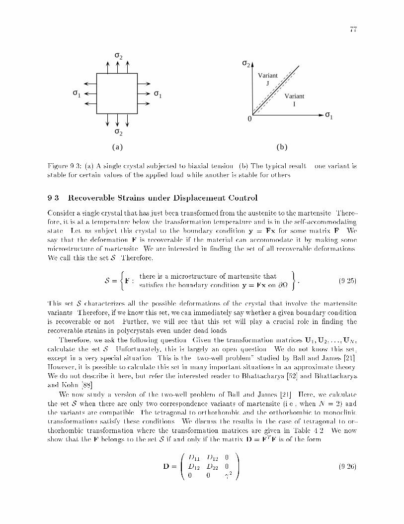
77

σ2

0σ1

σ2

σ1

VariantJ

VariantI

σ2

σ1

(a) (b)

Figure 9.3: (a) A single crystal subjected to biaxial tension. (b) The typical result one variant isstable for certain values of the applied load while another is stable for others.

9.3 Recoverable Strains under Displacement Control

Consider a single crystal that has just been transformed from the austenite to the martensite. There-fore, it is at a temperature below the transformation temperature and is in the self-accommodatingstate. Let us subject this crystal to the boundary condition y = Fx for some matrix F. Wesay that the deformation F is recoverable if the material can accommodate it by making somemicrostructure of martensite. We are interested in nding the set of all recoverable deformations.We call this the set S. Therefore,

S =

(F :

there is a microstructure of martensite thatsatises the boundary condition y = Fx on @

): (9.25)

This set S characterizes all the possible deformations of the crystal that involve the martensitevariants. Therefore, if we know this set, we can immediately say whether a given boundary conditionis recoverable or not. Further, we will see that this set will play a crucial role in nding therecoverable strains in polycrystals even under dead loads.

Therefore, we ask the following question. Given the transformation matrices U1;U2; : : : ;UN ,calculate the set S. Unfortunately, this is largely an open question. We do not know this set,except in a very special situation. This is the \two-well problem" studied by Ball and James [21].However, it is possible to calculate this set in many important situations in an approximate theory.We do not describe it here, but refer the interested reader to Bhattacharya [52] and Bhattacharyaand Kohn [88].

We now study a version of the two-well problem of Ball and James [21]. Here, we calculatethe set S when there are only two correspondence variants of martensite (i.e., when N = 2) andthe variants are compatible. The tetragonal to orthorhombic and the orthorhombic to monoclinictransformations satisfy these conditions. We discuss the results in the case of tetragonal to or-thorhombic transformation where the transformation matrices are given in Table 4.2. We nowshow that the F belongs to the set S if and only if the matrix D = FTF is of the form

D =

0B@ D11 D12 0D12 D22 00 0 2

1CA (9.26)

78

D

D - D

12

11 22α − β2 β − α2 2 2

F+λ

F -λ

Fλ,µ(U )1 (U )2

Figure 9.4: The shaded region shows all the boundary conditions that can be satised by mi-crostructures of the two variants of martensite in a tetragonal to orthorhombic transformation.

and D11; D12; D22 satisfy the following conditions

D11D22 D212 = 22

D11 +D22 + 2D12 2 + 2

D11 +D22 2D12 2 + 2

: (9.27)

The numbers D11; D12; D22 that satisfy these conditions lie on a portion of a surface in D11 D12 D22 space. A projection of this set is shown in Fig. 9.4. Notice that Eq. (9.27)1 describessome innite surface in this space while the inequalities in Eq. (9.27)2;3 place some restrictionson it. Consequently, this set looks like an orange peel or half an \American football". We haveshown a attened version of this set in Fig. 9.4 by projecting it onto the (D11D22)D12 plane.The shaded region describes the set of all deformations that can obtained using microstructures ofmartensite. The left-most corner corresponds to the pure variant U1 while the right-most cornercorresponds to the pure variant U2.

Let us now try to prove this result. We begin by showing that any matrix F in S satises theconditions stated above. We do so by using the average compatibility conditions derived in Sec. 8.1.Let the microstructure that meets the boundary condition F involve the matrices F1;F2; : : : ;FM

in the volume fraction 1; 2; : : :M . Since this is a microstructure of martensite, each matrixFm = QmUI ; I = 1 or 2 for some rotation matrix Qm. We begin by showing that D is of the formEq. (9.26). We obtain from Eq. (8.3)1 that

Fe3 =MXm=1

(mFme3) (9.28)

However, each matrix Fm = QmUI and U1e3 = U2e3 = e3. Therefore,

Fe3 = Me3 where M =MX

m=1

mQm: (9.29)

79

Let us hold this information for a while. Notice that detFm = detU1 for each m and hence wecan use Eq. (8.4) to conclude that

FT e3 =MX

m=1

mFTm e3: (9.30)

However,

FTm e3 = (QmUI)T e3 = QmU

1I e3 =

1

Qme3: (9.31)

Therefore,

FT e3 =1

Me3 (9.32)

where the matrix M is dened earlier in Eq. (9.29). Putting Eq. (9.29) and Eq. (9.32) together, weconclude that

De3 = FTFe3 = FT ( Me3) = FT ( 2FT e1) = 2e3: (9.33)

This implies that D33 = 2; D13 = D23 = 0 which is the same as Eq. (9.26).We now turn to Eq. (9.27)1. Since detFm = U1 = for each m, it follows from Eq. (8.3)3

thatdetF = so that detD = 22 2: (9.34)

However, taking the determinant of D in Eq. (9.26),

detD = 2(D11D22 D212) (9.35)

and we obtain Eq. (9.27)1.We nally turn to Eq. (9.27)2 and Eq. (9.27)3. For any vector e we obtain from Eq. (8.3)1 that

Fe =MX

m=1

(mFme); and hence, e De = jFej2 MX

m=1

(mjFmej2) = maxI=1;2

(e U2I e) (9.36)

as in Sec. 9.1. We obtain Eq. (9.27)2 by substituting e =1p2(e1+e2) and Eq. (9.27)3 by substituting

e = 1p2(e1 e2). Therefore, we have shown that every matrix F 2 S satises Eq. (9.26) and Eq.

(9.27).We now show the converse. In other words, we show that every matrix F that satises Eq.

(9.26) and Eq. (9.27) is automatically in S. In other words, if F satises these conditions, we cannd a microstructure of martensite that satises homogeneous boundary conditions y = Fx. Wedo so by constructing twins within twins. Here, we present the ideas behind the calculation, butomit the details.

According to Sec. 5.6, there are two solutions to the twinning equation QU2 U1 = a n.Let us call these solutions fQ1; a1; n1g and fQ2; a2; n2g. Let us form ne twins between the twovariants using the rst solution. This has average deformation gradient equal to

F+ = (Q1U2) + (1 )U1 = U1 + a1 n1: (9.37)

As goes from 0 to 1, the point corresponding to F+ in Fig. 9.4, travels from the left corner to

the right corner using the upper boundary. Similarly, if we construct ne twins using the secondsolution, the average deformation

F = U1 + a2 n2: (9.38)

80

travels from the left to the right corner using the lower boundary. Further, it is possible to showthat for each , there is a solution to the equation

QF F+

= a n: (9.39)

Therefore we can form a twin-within-twin microstructure using alternating bands of F+ and F in

the volume fraction . This has average deformation gradient

F(;) = QF + (1 )F+

: (9.40)

As goes from 0 to 1, the point corresponding to F(;) in Fig. 9.4, travels from the point corre-

sponding to F+ on the upper boundary to the point corresponding to F on the lower boundary.

Therefore, by varying and between 0 and 1, we can cover the entire shaded region in Fig. 9.4.

10 Polycrystals

So far, we have studied the martensitic transformation and the shape-memory eect in singlecrystals. However, typical commercial specimens are polycrystalline. Experimental observationssuggest that there can be signicant dierence in the shape-memory eect between single andpolycrystals. Some materials have a large recoverable strain as single crystals, but little or noneas polycrystals; while others have a large recoverable strain even as polycrystals. Here are threeexamples.

1. Ni-37Al (at.%) Transformation: Cubic to tetragonal. Enami et al. [90] report that singlecrystals can recover tensile strains ranging from 0 to 13% depending on orientation. However,polycrystals are greatly susceptible to intergranular fracture in tension, while in compressionKim and Wayman [91] report that polycrystals can recover only about 0.2% strains.

2. Cu-14Al-4Ni (wt.%) Transformation: Cubic to orthorhombic or monoclinic-II. Eucken andHirsch [92] report that polycrystalline ribbons with uncontrolled texture recover only about2.5% tensile strain while specially textured polycrystalline ribbons fully recover about 6.5%tensile strain. Single crystals recover tensile strains ranging from 2 to 9% depending onorientation.

3. Ti-50.6Ni (at.%) Transformation: Cubic to monoclinic-I. This material is very widely usedcommercially. Ling and Kaplow [93, 94] report that drawn polycrystalline wires fully recoverfrom 4 to 8% strain depending on deformation mode, processing and manufacturer. Similarobservations have been published by others [95, 96, 97, 98]. Single crystals recover tensilestrains ranging from 3 to 10% depending on orientation [98, 99].

Bhattacharya and Kohn [88] studied this problem using an approximate theory. In particular,they estimated the recoverable strains in polycrystals. They found that the set of recoverabledeformations in a polycrystal depends not only on the transformation strain and the texture of thepolycrystal, but critically on the change of symmetry during the transformation. Brie y, greaterthe change in symmetry during the underlying transformation, greater the recoverable strains.Notice that this is consistent with the examples above: NiAl undergoes a cubic to tetragonaltransformation, CuAlNi undergoes a cubic to orthorhombic or monoclinic transformation and NiTiundergoes a cubic to monoclinic transformation. We now give a brief overview of their analysis byextending the theory we have developed to polycrystals.

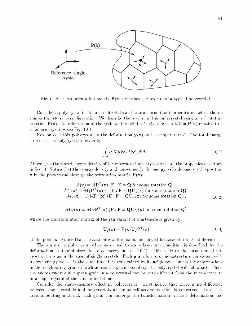
81

P(x)

Reference singlecrystal

x

Figure 10.1: An orientation matrix P(x) describes the texture of a typical polycrystal.

Consider a polycrystal in the austenite state at the transformation temperature. Let us choosethis as the reference conguration. We describe the texture of this polycrystal using an orientationfunction P(x): the orientation of the grain at the point x is given by a rotation P(x) relative to areference crystal see Fig. 10.1.

Now subject this polycrystal to the deformation y(x) and a temperature . The total energystored in this polycrystal is given by Z

'(ry(x)P(x); )dV: (10.1)

Above, ' is the stored energy density of the reference single crystal with all the properties describedin Sec. 4. Notice that the energy density and consequently the energy wells depend on the positionx in the polycrystal through the orientation matrix P(x):

A(x) = APT (x) fF : F = Q for some rotation Qg ;M1(x) =M1P

T (x) = fF : F = QU1(x) for some rotation Qg ;M2(x) =M2P

T (x) fF : F = QU2(x) for some rotation Qg ;...

MN(x) =MNPT (x) fF : F = QUN (x) for some rotation Qg

(10.2)

where the transformation matrix of the Ith variant of martensite is given by

UI(x) = P(x)UIPT (x) (10.3)

at the point x. Notice that the austenite well remains unchanged because of frame-indierence.The state of a polycrystal when subjected to some boundary condition is described by the

deformation that minimizes the total energy in Eq. (10.1). This leads to the formation of mi-crostructures as in the case of single crystals. Each grain forms a microstructure consistent withits own energy wells. At the same time, it is constrained by its neighbors unless the deformationsin the neighboring grains match across the grain boundary, the polycrystal will fall apart. Thus,the microstructure in a given grain in a polycrystal can be very dierent from the microstructurein a single crystal of the same orientation.

Consider the shape-memory eect in polycrystals. First notice that there is no dierencebetween single crystals and polycrystals as far as self-accommodation is concerned. In a self-accommodating material, each grain can undergo the transformation without deformation and

82

hence the polycrystal can undergo the transformation without deformation. Furthermore, there isno mismatch between the grains. This in turn implies that self-accommodation prevents residualstresses in a polycrystalline material. This rules out the possibility of using texture as a means ofcreating a \two-way shape-memory eect".

On the other hand, recoverable strains can be signicantly dierent. Consider a self-accommodatedpolycrystal of martensite and deform it. Each grain tries to accommodate the deformation by form-ing its own microstructure. However, it is constrained by its neighbors. Therefore, the situation ismuch more complicated than in the single crystals. For example, consider uniaxial tension underload control as in Sec. 9.2.1. In a single crystal, we obtained the recoverable strain by simply ndingthe variant with the maximal extension in the direction of loading. So in a polycrystal, we couldnd the strain of the optimal variant in each grain and take the average over all grains. However,this procedure leads to a wrong answer. In particular, it overestimates the actual recoverable strain.Consider two neighboring grains. Assume that each forms its optimal variant. Unless the orien-tations of the grains are related in a very special way, there will be a mismatch across the grainboundary. In order to prevent this mismatch, the grains can not form their optimal variants. SeeMiyazaki et al [100, 101] for experimental observations of this fact in carefully prepared bicrystals.Therefore, in a polycrystal, we have to nd the optimal microstructure that respects the constraintsbetween the grains. This requires a more general approach similar to Sec. 9.2.2.

Recall that a single crystal has a set of recoverable deformations S dened in Eq. (9.25). It isexactly those deformations that a single crystal can accommodate by making a microstructure ofmartensite. Similarly, let us dene a set of recoverable deformations of a polycrystal P as the setof all possible coherent deformations that can be accommodated in each grain by a microstructureof martensite. Each grain in the polycrystal has its own set of recoverable deformations S(x).We can obtain this from the set S through the orientation matrix P(x); i.e., S(x) = SPT (x).Therefore, a recoverable deformation in a polycrystal is coherent and satises ry(x) 2 S(x) foreach x. Therefore, we obtain

P =

(F :

there is a coherent deformation y which is recoverable in each grainand satises the boundary condition y = Fx on @

)

=

(F :

there is a coherent deformation y such that ry(x) 2 S(x)and it satises the boundary condition y = Fx on @

):

(10.4)

There is a very easy estimate one can obtain. This is the so-called Taylor bound T . Here, weassume that each grain undergoes the same macroscopic deformation. Therefore, a deformation isrecoverable according to the Taylor bound if it is recoverable in each grain. Therefore,

T =\x2

S(x) = fF : FP(x) 2 S for each x 2 g : (10.5)

The physical meaning of the Taylor bound is clear. It describes the strains that can be accom-modated without making use of any cooperative eects between the grains. Therefore, the Taylorbound underestimates the actual recoverable strains.

Recall from Sec. 9.3 that we were able to calculate the set S only for very special transfor-mations, but were unable to do so for the most interesting cases. Therefore, we are unable tocalculate the set P or even the set T . Instead, Bhattacharya and Kohn [88] used an approximategeometrically linear theory to calculate the set T . They also argued [102] that the Taylor boundis a surprisingly good indicator of the actual set of recoverable deformations. Based on this theyconcluded the following. In a cubic to tetragonal or a cubic to trigonal transformation, the range

83

of deformations that each grain can undergo by rearranging variants is too small to allow cooper-ative deformation between the grains. Hence, the recoverable deformations have negligible straincompared to the self-accommodated state and hence, they have little or no recoverable strain. Incontrast, in alloys that undergo cubic to monoclinic transformation, the large change in symmetryprovides a great range of deformations by rearranging variants, and allowing cooperative deforma-tion between strains. Hence, we expect signicant recoverable strains. Alloys that undergo cubicto orthorhombic transformation lie somewhere in between. See [88] for further details and also adetailed comparison with experiment.

11 Summary

Let us quickly review some of the main ideas and results.

1. A change in symmetry during transformation causes the material to have a number of variants.In particular, if the austenite has greater symmetry than the martensite, we have one variantof austenite and multiple variants of martensite. We can calculate the number of variantsbased on the change in symmetry. The transformationmatrix of each variant can be calculatedfrom the lattice parameters.

2. The energy density of such materials has multiple wells each well associated with one variant.

3. Energy minimization with a multi-well energy naturally leads to ne-scale microstructure.We can calculate various aspects of this microstructure based on the change in symmetry andlattice parameters.

4. We can represent a coherent microstructure using a (weakly converging) sequence of defor-mations.

5. We can derive the crystallographic theory of martensite based on energy minimization. Basedon this, we can calculate all the possible austenite-martensite interfaces. However, this pre-sentation does not require an a priori knowledge of the twinning modes; these as well as thetwinning elements can be calculated from the change in symmetry and the transformationmatrix.

6. The microstructure, and consequently the macroscopic properties, can depend very delicatelyon lattice parameters. For example, the wedge-shaped microstructure which is important forreversibility requires that the lattice parameters satisfy rather strict conditions.

7. Only materials with cubic austenite that undergo a volume preserving transformation willdisplay the shape-memory eect.

8. It is not possible to induce the two-way shape-memory eect by making specially texturedpolycrystals.

9. The average compatibility conditions are a very useful tool in studying general questions ofmicrostructure, like self-accommodation.

10. The shape-memory behavior of polycrystals depends not only on the transformation strain andtexture, but critically on the change of symmetry in the underlying transformation. Brie y,there is no shape-memory eect if the change in symmetry is small (cubic to tetragonal ortrigonal). On the other hand, there is some recoverable strain when the change in symmetryis large (cubic to orthorhombic or monoclinic).

84

11. Shape-memory eect in cubic to tetragonal alloys requires very special texture. Even then,it will have imperfect recoverablity.

12. Materials undergoing a cubic to monoclinic transformation will display the signicant shape-memory eect.

13. All these predictions agree with experimental observations.

14. Finally, there are many open problems in this theory. The most important is our inabilityto calculate the set of recoverable strains in a single crystal except in a most simple exampleusing the exact theory.

Acknowledgment

I am deeply indebted to Richard D. James for introducing me to this subject and for continuingto inspire me. This chapter draws from the research that I have been involved in as a graduatestudent of Richard D. James at the University of Minnesota, as a post-doc with Robert V. Kohnat the Courant Institute of Mathematical Sciences and also at Caltech. I gratefully acknowledgethe nancial support from the Air Force Oce of Scientic Research ( while at Minnesota andCaltech), the Army Research Oce (while at Courant), the National Science Foundation (while atMinnesota, Courant and Caltech) and the Oce of Naval Research (while at Caltech) during theseyears. I thank Ms. Cecilia Lin for her patient help with the gures.

References

[1] G.B. Olson and W.S. Owen (Editors), Martensite, ASM (1992).

[2] R. Gotthardt and J. Van Humbeeck (Editors), Proceedings of the International Conferenceon Martensitic Transformations: ICOMAT-95, J. de Phys. 1V 5 Colloque C8 (1995).

[3] T. Saburi and S. Nenno, In \Phase transformations" (ed. H.I Aaronson, D.E. Laughlin, R.F.Sekerka and C.M. Wayman), The Metallurgical Society of AIME, 1455 (1981).

[4] T. Tadaki, K. Otsuka and K. Shimizu, Annual Rev. Mat. Sci. 18, 25 (1988).

[5] S. Miyazaki and K. Otsuka, ISIJ International 29, 353 (1989).

[6] C.M. Wayman, Prog. Mat. Sci. 36, 203 (1992).

[7] C.M. Wayman, Introduction to the Crystallography of Martensitic Transformations, Macmil-lan (1964).

[8] J.M. Ball and R.D. James, The Mathematics of Microstructure, Birkhauser, To appear (1997).

[9] M.S. Wechsler, D.S. Lieberman and T.A. Read, Trans AIME J. Metals 197, 1503 (1953).

[10] J.S. Bowles and J.K. MacKenzie, Acta Metall. 2, 129 (1954).

[11] J.M. Ball and R.D. James, Arch. Rat. Mech. Anal. 100, 13 (1987).

[12] M.E. Gurtin, An introduction to continuum mechanics, Academic Press (1981).

[13] A.J.M. Spencer, Continuum mechanics, Longman (1980).

[14] Y.C. Fung, A rst course in continuum mechanics, Prentice-Hall (1977).

[15] J.L. Ericksen, J. Appl. Mech. 45, 740 (1978).

[16] J.L. Ericksen, Arch. Rat. Mech. Anal. 72, 1 (1979).

[17] J.L. Ericksen, Arch. Rat. Mech. Anal. 73, 99 (1980).

85

[18] J.L. Ericksen, In \Phase Transformations and Material Instabilities in Solids" (ed. M.E.Gurtin), Academic Press, 61 (1984).

[19] M. Pitteri, J. Elasticity 14, 175 (1984).

[20] G.P. Parry, Math. Proc. Cambridge Phil. Soc. 80, 189 (1976).

[21] J.M. Ball and R.D. James, Phil. Trans. Royal Soc. London A 338, 389 (1992).

[22] R.L. Fosdick and B. Hertog, Arch. Rat. Mech. Anal 110, 43 (1990).

[23] M. Pitteri, J. Elasticity 15, 3 (1985).

[24] R.D. James, In \Metastability and Incompletely Posed Problems" (ed. S. Antman, J.L. Er-icksen, D. Kinderlehrer and I. Muller) IMA Vol. 3, Springer Verlag, 147 (1987).

[25] D.S. Lieberman, M.A. Schmerling and R. S. Karz, In \Shape Memory Eect in Alloys" (ed.J. Perkins), Plenum Press 203 (1975).

[26] K. Bhattacharya, R.D. James and P.J. Swart, To appear in Acta Materialia (1997).

[27] L. Guttman, Trans. AIME J. Metals 188, 1472 (1950).

[28] M.J. Duggin and W.A. Rachinger, Acta Metall. 12, 529 (1964).

[29] K.M. Knowles and D.A. Smith, Acta Metall. 29, 101 (1981).

[30] K. Bhattacharya, In preparation.

[31] K. Enami and S. Nenno, Metall. Trans. 2, 1487 (1971).

[32] T. Tadaki, K. Katsuki and K. Shimizu, Suppl. Trans. Japan Inst. Metals 17, 187 (1976).

[33] H. Okamoto, M. Oka, I. Tamura, Trans. Japan Inst. Metals 19, 674 (1978).

[34] N.H. Andersen, B. Lebech and H.F. Poulsen, Physica C 172, 31 (1990).

[35] L.C. Chang and T.A. Read, Trans. AIME J. Metals 191 47 (1951).

[36] H.K. Birnbaum and T.A. Read, Trans. Metall. Soc. AIME 218, 661 (1960).

[37] S. Chakravorty and C.M. Wayman, Acta Metall. 25, 989 (1977).

[38] S. Matsumoto, A. Sato and T. Mori, Acta Metall. Mater. 42 1207 (1994).

[39] I. Fonseca, J. Math. Pures et Appl. 67, 175 (1988).

[40] Yu.G. Reshetnyak, Siberian Math J. 8, 631 (1967).

[41] R.W. Cahn, Adv. in Physics 3 363 (1954).

[42] M.V. Klassen-Neklyudova, Mechanical Twinning of Crystals, Consultants Bureau (1964).

[43] A. Kelly and G.W. Groves, Crystallography and Crystal Defects, Addison-Wesley (1970).

[44] M. Pitteri, Arch. Rat. Mech. Anal. 88, 25 (1985).

[45] A.G. Khachaturyan, Theory of structural transformations in solids, John Wiley and Sons(1983).

[46] M. Pitteri and G. Zanzotto, Continuum Theories for Phase Transitions and Twinning inCrystals, Chapman and Hall, To appear (1997).

[47] J.L. Ericksen, J. Thermal Stresses 4, 107 (1981).

[48] J.L. Ericksen, Arch. Rat. Mech. Anal. 88, 337 (1985).

[49] M.E. Gurtin, Arch. Rat. Mech. Anal. 84, 1 (1983).

[50] K. Bhattacharya, Arch. Rat. Mech. Anal. 120, 201 (1992).

[51] N.K. Simha, J. Mech. Phys. Solids 45, 261 (1997).

[52] K. Bhattacharya, Cont. Mech. Thermodyn. 5, 205 (1993).

[53] C. Chu, PhD thesis, Univ. Minnesota (1993).

[54] M. Nishida, K. Yamauchi, I. Itai, H. Ohgi and A. Chiba, Acta Metall. Mater. 43, 1229 (1995).

[55] K. Bhattacharya, In \Contemporary research in the mechanics and mathematics of materials"(ed. R.C. Batra and M.F. Beatty), CIMNE, 251 (1996).

86

[56] L.C. Young, Lectures on the Calculus of Variations and Optimal Control Theory, Chelsea(1980).

[57] M. Chipot and D. Kinderlehrer, Arch. Rat. Mech. Anal 103, 237 (1988).

[58] J.M. Ball, In \Nonlinear analysis and mechanics: Heriot-Watt symposium Vol. 1" PitmanRes. Notes in Math. 17, 187 (1977).

[59] B. Dacarogna, Direct Methods in the Calculus of Variations, Springer-Verlag (1989).

[60] L.C. Evans, Weak Convergence Methods for Nonlinear Partial Dierential Equations, CMBS74, American Mathematical Society (1990).

[61] M.W. Burkart and T.A. Read, Trans. AIME J. Metals 197, 1516 (1953).

[62] G. Arlt, J. Mat. Sci. 22, 2655 (1990).

[63] R.V. Kohn and S. Muller, Phil. Mag. A 66, 697 (1992).

[64] J.M. Ball, P.J. Holmes, R.D. James, R.L. Pego and P.J. Swart, J. Nonlinear Sci. 1, 17 (1990).

[65] K.A. Bywater and J.W. Christian, Phil. Mag. 25, 1249 (1972).

[66] S. Miyazaki, Private communication (1994).

[67] K. Otsuka and K. Shimizu, Trans. Jap. Inst. Metals 15, 103, 109 (1974).

[68] K. Okamoto, S. Ichinose, K. Morii, K. Otsuka and K. Shimizu, Acta Metall. 34, 2065 (1986).

[69] C. Chu and R.D. James, J. de Phys. IV 5, Colloque C8 143 (1995).

[70] K. Otsuka and K. Shimizu, Japan J. Appl. Phys. 8, 1196 (1969).

[71] S.S. Tan and H.B. Xu, Cont. Mech. Thermodyn. 2, 241 (1990).

[72] S. Chakravorty and C.M. Wayman, Metall. Trans7A, 555, 569 (1976).

[73] K. Adachi and C.M. Wayman, Metall. Trans. 16A, 1567, 1581 (1985).

[74] K. Bhattacharya, Acta Metall. Mater. 39, 2431 (1991).

[75] K. Hane, PhD Thesis, Univ. Minnesota, In preparation (1997).

[76] C.B. Morrey, Multiple Integrals in the Calculus of Variations, Springer-Verlag (1966).

[77] T. Saburi and C.M. Wayman, Acta Metall. 27, 979 (1979).

[78] R.D. James and D. Kinderlehrer, In \Partial Dierential Equations and Continuum Modelsof Phase Transitions" (ed. M. Rascle, D. Serre and M. Slemrod), Lecture Notes in Physics344 Springer-Verlag, 51 (1989).

[79] K. Bhattacharya, N. Firoozye, R.D. James and R.V. Kohn, Prof. Royal Soc. Edin. 124 A,843 (1994).

[80] J. L. Ericksen, Arch. Rat. Mech. Anal 10, 189 (1962).

[81] F. Murat and L. Tartar, In \Recent Methods in Nonlinear Analysis" (ed. E. De Giorgi, E.Magenes and U. Mosco), Pitagora, 245 (1979).

[82] M. Avellaneda, A.V. Cherkaev, K.A. Lurie and G.W. Milton, J. Appl. Phys 63, 4989 (1988).

[83] J.M. Ball, In \Partial Dierential Equations and Continuum Models of Phase Transitions"(ed. M. Rascle, D. Serre and M. Slemrod), Lecture Notes in Physics 344 Springer-Verlag, 207(1989).

[84] L. Tartar, In \Nonlinear Analysis and Mechanics" (ed. R.J. Knops), Pitman Research Notes39, 136 (1978).

[85] D. Kinderlehrer and P. Pedregal, Arch. Rat. Mech. Anal. 115, 329 (1991).

[86] H. Tas, L. Delaey and A. Deruyterre, Metall. Trans 4, 2833 (1973).

[87] R.D. James, J. Mech. Phys. Solids 34, 359 (1986).

[88] K. Bhattacharya and R.V. Kohn, Acta Mater. 44, 529 (1996).

[89] R. Abeyaratne, C. Chu and R.D. James, Phil. Mag A 73, 457 (1996).

87

[90] K. Enami, V.V. Martynov, T. Tomie, L.G. Khandros, and S. Nenno, Trans. Japan Inst.Metals 22, 357 (1981).

[91] Y.D. Kim and C.M. Wayman, Metall. Trans. A 23A, 2981 (1992).

[92] S. Eucken and J. Hirsch, Mat. Sci. Forum 56-58, 487 (1990).

[93] H.C. Ling and R. Kaplow, Metall. Trans. A 12A, 2101 (1981).

[94] H.C. Ling and R. Kaplow, Mat. Sci. Engng. 48, 241 (1981).

[95] S. Miyazaki, K. Otsuka and Y. Suzuki, Scripta Metall. 15, 287 (1981).

[96] M. Piao, K. Otsuka, S. Miyazaki and H. Horikawa, Mat. Trans Japan Inst. Metals 34, 919(1993).

[97] T. Saburi, T. Tatsumi and S. Nenno, J. de Phys. 43, Colloque C4 261 (1982).

[98] T. Saburi, M. Yoshida and S. Nenno, Scripta Metall. 18, 363 (1984).

[99] S. Miyazaki, S. Kimura, K. Otsuka and Y. Suzuki, Scripta Metall. 18, 883 (1984).

[100] S. Miyazaki, T. Kawai and K. Otsuka, J. de Phys. 43, Colloque C4 813 (1982).

[101] S. Miyazaki, T. Kawai and K. Otsuka, Scripta Metall. 16, 431 (1982).

[102] K. Bhattacharya and R.V. Kohn, To appear in Arch. Rat. Mech. Anal. (1997).