The numerical solution of the pressure Poisson equation

for the incompressible Navier-Stokes equations using a

quadrilateral spectral multidomain penalty method

J. A. Escobar-Vargasa,∗, P. J. Diamessisa, C. F. Van Loanb

aSchool of Civil and Environmental Engineering, Cornell University, Ithaca, NY 14853bDepartment of Computer Science, Cornell University, Ithaca, NY 14853

Abstract

We outline the basic features of a spectral multidomain penalty method (SMPM)-based solver for the pressure Poisson equation (PPE) with Neumann bound-ary conditions, as encountered in the time-discretization of the incompressibleNavier-Stokes equations. One one hand, the SMPM discretization enables ro-bust under-resolved simulations without sacrificing high accuracy. On the other,the solution of the PPE is an inevitable requirement when simulating stronglynon-hydrostatic flows, such as those occuring in the natural environment. Thefundamental building blocks of the PPE solver presented here are a Kronecker(tensor) product-based computation of the left null singular value of the non-symmetric SMPM-discretized Laplacian matrix and a custom-designed two-levelpreconditioner. Both of these tools are essential towards ensuring existence anduniqueness of the solution of the discrete linear system of equations and enablingits efficient iterative calculation. The accuracy and efficiency of the PPE solverare demonstrated through application to two incompressible flow benchmarks,the Taylor vortex and the Lid-driven cavity flow. In addition to providing anefficient tool for the iterative solution of the PPE in incompressible flow simu-lations, this work presents algorithms which are of interest to the subdisciplineof the numerical linear algebra community focused on the iterative solution ofconsistent singular non-symmetric linear systems of equations.

Keywords: Computational fluid dynamics, Pressure Poisson equation,Neumann boundary conditions, Spectral multidomain method, Non-symmetricmatrices, Singular consistent system, Singular value decomposition, Two-levelpreconditioner.

∗Jorge A. Escobar-Vargas, School of Civil and Environmental Engineering, Cornell Uni-versity, Ithaca, NY 14853, U.S.A. . email: jae47@cornell.edu

Preprint submitted to Journal of Computational Physics December 5, 2011

1. Introduction

Spectral multidomain penalty methods (SMPM) [1, 2, 3] are a class of dis-continuous higher-order (spectral) accuracy element-based discretization tech-niques designed to have superior numerical stability properties as compared toequivalent continuous methods, such as the spectral element (SEM) and spec-tral multidomain methods [4, 5, 6, 7]. SMPM consist of collocating a linearcombination of the governing equation and boundary or patching (subdomaincommunication) conditions, the latter multiplied by a penalty coefficient, atthe boundaries or subdomain interfaces, respectively. Numerical stability atthe subdomain interfaces is thereby enabled by weakly enforcing the bound-ary/patching conditions, leading to a weakly discontinuous solution at the sub-domain interfaces. In this regard, the SMPM strongly resembles the discontin-uous Galerkin method (DGM) [8, 9]. However, the former is a collocation-basedformulation, whereas the latter works with a weighted residual nodal Galerkinformulation with appropriately specified numerical fluxes specified at the sub-domain interfaces.

The enhanced numerical stability of SMPM and DGM, combined with the ex-ponential convergence, near-negligible artificial dissipation and dispersion andspatial adaptivity of element-based higher-order discretization techniques, makethem particularly attractive as a computational tool for under-resolved fluidflow simulations. One class of fluid flow phenomena where under-resolved fluidflow simulations are inevitable are smaller-scale environmental stratified flowprocesses, such as localized turbulent bursts [10] and internal solitary waves[11]. Such phenomena are subject to a very broad scale separation and stronglynonlinear and non-hydrostatic dynamics. Currently available computationalresources allow the simulation of only the larger, energetic scales of an envi-ronmental turbulent flow with the smaller, more viscously-dominated, scalesremaining unresolved [12]. The accurate reproduction of internal solitary waveevolution requires the adequate resolution of the steep waveform, a direct resultof the waves’ strong nonlinearity, without over-resolving the wave interior toallow for a sufficiently large domain for the wave to propagate within [13].

The DGM has been applied primarily to the study of mesoscale phenomena(of scale O(10 to 100km ) ) in the ocean and atmosphere [14, 15], where therelevant dynamics are governed by the compressible Navier-Stokes equations(NSE), a hyperbolic system of equations, for which the DGM is ideally suited[8]. However, smaller-scale environmental stratified flow processes are inherentlyincompressible [16]. Moreover, they are strongly non-hydrostatic and containsignificant vertical accelerations, including the vertical pressure gradient termwhich cannot be neglected. In the case of internal solitary waves, in particu-lar, non-hydrostatic effects provide the necessary physical dispersion that allowthese waves to maintain their steep waveform over large propagation distances.Invoking the hydrostatic assumption, typically used in larger-scale geophysicalflow modeling [17], will force the simulation to produce highly erroneous phys-

2

ical results. One must solve numerically either the Poisson or Stokes equation[18] that arises when treating the pressure in an non-hydrostatic incompressibleflow simulation [19].

Although DGM solvers of the incompressible NSE [20, 21] have been reported inthe literature, none have been applied to strongly under-resolved incompressibleflow simulations, including those of environmental stratified flows. In contrast,a SMPM model has been developed and used by the second author of this paperfor high Reynolds number incompressible stratified turbulent flows in domainswith one non-periodic direction (the vertical) [22, 23, 12]. One-dimensionalspectral subdomains, based on Legendre polynomials, are used in the vertical.The computational domain is a rectangular box the with periodic horizontaldirections which used a Fourier polynomial discretization.

The time-discretization, originally proposed by Karniadakis and co-workers [24](hereafter referred to as KIO), used in the above SMPM model requires the solu-tion of a Poisson equation for the pressure with Neumann boundary conditions.However, solution of this Poisson equation is only required for the horizontalzero Fourier mode. In practice, on account of incompressibility and the use ofrigid and impermeable top and bottom boundaries, the zero Fourier mode forthe pressure mode is directly set to zero and the corresopnding linear system ofequations does not have to be solved.

Should more complex domain geometries and non-periodic streamwise bound-ary conditions be necessary, a quadrilateral spectral subdomain discretization[3] is needed. In the context of the KIO time discretization, the solution ofthe above Poisson-Neumann problem for the pressure is now inevitable. More-over, on account of the broad range of scales in environmental stratified flowprocesses, any associated simulation will involve a very large number of degreesof freedom (DOF) and the numerical solution of the linear system of equationscorresponding to the pressure Poisson equation (PPE) can only be performediteratively.

The matrix resulting from the SMPM discretization of the Poisson-Neumannproblem is ill-conditioned for two reasons: a) the inherent ill-conditioning ofhigher-order interpolating polynomials and b) the ill-posedness of the corre-sponding analytical equation, whose solution can only be determined up toan additive constant. Both of these factors pose significant challenges to theiterative solution of the PPE. Moreover, existence of a solution requires the sat-isfaction, at the spatially analytical level, of an integral compatibility conditionbetween boundary conditions and right hand side of the PPE [25]. In the KIOscheme, the compatibility condition is inherently satisfied at the spatially con-tinuous level [24]. However, under-resolution and the presence of the penaltyterms can cause a violation of the compatibility condition (see reference [26]and §5.3 of this paper), thereby posing an additional major challenge to theiterative solution of the PPE.

3

The above challenges in the iterative solution of the linear system associatedwith the PPE, or the Stokes equation resulting from alternative time discretiza-tions of the incompressible NSE [18], have been efficiently addressed through thedevelopment of appropriate preconditioning techniques [27, 28, 29]. All thesetechniques are designed for the symmetric matrices resulting directly from theGalerkin formulation of SEM. Extensive background on the numerical solutionof symmetric linear systems of equations can already be found in the numericallinear algebra literature.

However, the matrix resulting from the SMPM discretization of the PPE isnon-symmetric on account of the use of a collocation discretization [7]. Whenexamining the numerical linear algebra literature, one observes a paucity of toolsfor preconditioning, matrix singularity treatment and solvability condition en-forcement (the matrix-level equivalent of the compatibility condition) for linearsystems with non-symmetric matrices.

Motivated by the above observations and the need to study environmental flowprocesses of increasing complexity, this paper presents strategies developed forthe efficient iterative solution of the SMPM-discretized PPE with Neumannboundary conditions resulting from application of the KIO splitting scheme tothe incompressible NSE. The fundamental building block of these strategies isa fast computation of the left null singular vector of the global Poisson ma-trix. Consistency of the associated linear system of equations, paramount tothe robust performance of the iterative GMRES solver, can only be ensured ifthis left null singular vector is available. In addition, a method for removingthe null singular value of the Poisson matrix is outlined, which also relies ofthe availability of the the left null singular vector. This method is contrasted,in terms of accuracy and robustness within the GMRES framework, to othermore commonly used techniques designed to ensure a unique solution to thePoisson-Neumann problem. A custom-designed two-level preconditioner is alsopresented and its superiority is demonstrated with respect to diagonal Jacobiand block-Jacobi preconditioners. Finally, the efficiency of the Poisson solver,as buttressed by all the above strategies, is assessed through its application tothe solution of two commonly considered benchmark problems.

2. Incompressible Navier-Stokes equations: temporal discretization

In this section we review the two time-discretization strategies, typicallyapplied by the higher-order method community to the incompressible Navier-Stokes equations [30]:

∂u

∂t+ u · ∇u =

1

ρ∇p+ ν∇2u+ F , (1)

∇ · u = 0 , (2)

4

where u is the velocity vector, ρ is the density, p is the pressure, ν is the kine-matic viscosity of the fluid, and F contains any additional forcing terms. Inthe case of environmental stratified flow processes, the forcing term accountsfor the restoring force of gravity in the vertical momentum equation, commonlyrepresented in the form of the Boussinesq approximation [31]. In what follows,we will neglect this term, as its role is not critical to the solution of the PPE.

The defining differences between possible temporal discretization strategies forequations in (1) and (2) are whether the the pressure gradient and viscousterms are coupled or not and whether boundary conditions are required for thepressure field. As a result, one may classify these strategies into main groups:Stokes-based solvers and fractional-time-stepping methods.

2.1. Stokes-based solvers

In this approach the non-linear terms are solved explicitly and treated asforcing terms (f) of a generalized Stokes problem [30], where the velocity andpressure are coupled through a discrete operator with the following structure

(H −BT

−B 0

)(u

p

)

=

(f

0

)

. (3)

In (3), H is the discrete analog of the Helmholtz operator, and B and BT

are the discretized gradient operator and divergence operators respectively [30].The Uzawa algorithm [18, 5] is used to solve this system of equations whichis modified such that a block upper triangular matrix is obtained and a blockback substitution is subsequently performed. This procedure decouples velocityfrom pressure at the discrete level. One of the well-documented challenges ofthis approach is the fulfillment of the inf-sup condition [32], which establishesthe coupling between velocity and pressure in order to satisfy existence anduniqueness (up to an additve constant) of the solution. In practical terms, ful-fillment of this condition necessitates a staggered grid, where the pressure fieldis approximated with a space of basis functions of lower degree than the oneused for the velocity, i.e. PN−2 vs PN . As a result, no boundary conditions arerequired for the pressure. As an alternative treatment of the inf-sup condition,a stabilization term can be added to the equations [33].

References [34, 27, 28, 18] discuss various preconditioning strategies used inthe numerical computation of the pressure component of the Stokes system ofequations. Such techniques typically rely on coarse grid preconditioners, fastdiagonalization method, additive Schwarz, and two-level preconditioners amongothers [18].

The time discretization associated with the Stokes equations and underlyingUzawa algorithm has been the foundation of a number of SEM-based investiga-tions of incompressible flows [35, 27], which include studies of environmental flow

5

processes [36, 37], where enhanced numerical stability is enabled through over-integration-based de-aliasing techniques [38]. However, penalty schemes have sofar been developed for single-variable partial differential equations, specificallythe advection-diffusion equation [1, 3] and adapted accordingly to the fractionalsteps of the KIO scheme for one-dimensional subdomains [22]. As a result,it is unclear how one might formulate a penalty scheme for the actual Stokesequations.

2.2. Fractional step methods

In projection methods, the velocity is decoupled from the pressure, the latterhaving the primary role of enforcing the incompressibility. As a result, a separatePoisson equation for the pressure must be solved. Here we describe a verycommonly used approach from this family of methods, the operator splittingscheme proposed by Karniadakis et. al [24],which is a more evolved, highertemporal accuracy, version of the scheme originally proposed by Chorin andTemam [30]. Whereas Chorin and Temam lump the viscous term and nonlinearterm in a single fractional step, with the nonlinear treated explicitly, and reservea separate step for the pressure, the KIO scheme allots the following independentfractional steps to each of the spatial terms in the right-hand side of (1):

v −∑Ji−1

q=0 αqvn−q

∆t=

Je−1∑

q=0

βqN(vn−q), (4)

ˆv − v

∆t= ∇pn+1, (5)

γ0vn+1 − ˆv

∆t= ν∇2vn+1, (6)

where v and ˆv are intermediate velocity fields. In the first fractional step, (4),the non-linear term is solved explicitly via a stiffly stable scheme [24], also re-garded as Adams-Bashforth/Backward Differentiation (AB/BDEk) [39]. In thesecond step, (5), a Poisson equation with Neumann boundary conditions has tobe solved for the pressure to enforce incompressibility by leading to an interme-diate velocity field ˆv that is divergence-free (∇ · ˆv = 0). Finally, in the thirdfractional step, (6), a modified Helmholtz equation is solved implicitly to obtainthe final velocity field (vn+1) at each time step. A more general and detailedanalysis of projection methods for incompressible flows is presented in [40] andspecifically for high-order methods in [30].

In its original presentation, the application and analysis of the KIO scheme isperformed in the framework of the SEM method [24]. As a result, no concernsarise in terms of the compatibility condition which is assumed to be satisfiednaturally. Moreover, to the best of our knowledge, there is no discussion in theliterature of issues with the singularity of the resulting Poisson matrix whicharise from the Neumann boundary conditions. Finally, efficient preconditioners

6

for the SEM-based KIO approach are based on a transformation of the expan-sion basis to a low-energy basis [29, 41], which is amenable to block diagonalpreconditioning.

Nonetheless, as is elaborated further in §5.2, application of an SMPM-basedspatial discretization to the incompressible NS equations within the KIO frame-work, poses concerns about Poisson matrix singularity and violation of a com-patibility condition. Moreover, an extension of preconditioners developed forcontinuous element-based schemes, such as SEM, and the associated symmetricPoisson matrix to the discontinuous collocation-based SMPM and the corre-sponding non-symmetric matrix is not a straightforward task. Identifying arobust framework for the iterative solution of the linear system of equations re-sulting from the SMPM-discretization pressure Poisson equation is the primaryobjective of this paper.

3. The pressure Poisson equation

3.1. Compatibility condition

In the KIO splitting scheme, the PPE is obtained by taking the divergenceof Eq. (5)

∇ ·ˆv − v

∆t= ∇ · ∇pn+1, (7)

and imposing a divergence-free condition to the intermediate velocity ˆv

∇ · ˆv = 0.

A Poisson equation with Neumann boundary conditions therefore results:

∇2p = ∇ ·

(

−v

∆t

)

= f on Ω, (8)

∂p

∂n= n ·

[Je−1∑

q=0

βqN(vn−q) + νβqL(vn−q)

]

= q on Γ. (9)

The above expression for the Neumann boundary condition q is used in the KIOscheme to ensure consistency with the AB/BDEk time-discretization of the in-compressible N-S equations [24].

The right hand side f and boundary operator q must satisfy a compatibil-ity condition for the PPE (Eq. (8)-(9)) to have a solution. Specifically, thePoisson-Neumann problem is compatible (solvable) only if the volume integral(area integral in two dimensions) of the right hand side is equal to the net fluxalong the boundaries, i.e. the boundary integral of the boundary conditions.By integrating Eq. (8) over the whole domain we obtain

∫

Ω

∇2p dΩ =

∫

Ω

f dΩ, (10)

7

and by employing Gauss’ theorem∫

Ω

∇2p dΩ =

∫

Γ

n · ∇p dΓ, (11)

∫

Ω

f dΩ =

∫

Γ

q dΓ. (12)

Therefore, the Poisson-Neumann problem (8)-(9) has a solution only if (12) issatisfied [24, 25, 42, 43]. As already indicated in §2.2, in the original presenta-tion of the KIO scheme, it is emphasized that the boundary integral of (11) istransformed by Gauss’ theorem into a volume integral where the divergence ofthe second term in the original integrand vanishes. As a result,

Je−1∑

q=0

βq

∫

Ω

∇ · (N)n−q dΩ =

∫

Ω

∇ ·

(v

∆t

)

dΩ (13)

must hold, which is indeed true through the AB/BDEk time-discretization, i.e.the compatibility condition is naturally satisfied.

3.2. Non-uniqueness of the pressure Poisson equation’s solution

In addition to the compatibility condition, the Poisson equation does nothave a unique solution because, by virtue of its boundary conditions, its solu-tion is some function plus an additive constant. That is, given the Neumannboundary conditions

n · ∇p = g onΓ, (14)

any function of the formp(x) = g(x) + h, (15)

where h is an indeterminate additive constant, satisfies the boundary conditions(9) and is a solution to the PPE. Of course, in the spatially continuous (ana-lytical) sense, once the pressure field has been obtained in the second fractionalstep of the KIO scheme, its determination up to an additive constant is a non-issue when computing ˆv through (5) since only the the gradient of the pressurefield (∇p) is required. However, for the spatially discretized version of the KIOscheme, the non-uniqueness of solution to the Poisson-Neumann problem gener-ates its own set of challenges as the corresponding linear system of equations isnearly-singular though consistent (provided the compatibility condition is satis-fied). The above challenges, in a numerical framework, of compability conditionsatisfaction and the non-uniqueness of the solution of the PPE motivate a closerlook at the SMPM discretization and its impact on the resulting Poisson matrixstructure.

4. The penalty-based discrete pressure Poisson equation

4.1. Spectral multidomain penalty method (SMPM)

Within each quadrilateral subdomain, on a Gauss-Lobatto-Legendre (GLL)grid, any function p(x, z, t) is approximated in nodal form as the tensor prod-uct of its Lagrange interpolating polynomials of degree N [3] in each spatial

8

dimension:

p(x, y, t) ≈N∑

i=0

N∑

j=0

p(xi, yj , t)li(x)lj(y), (16)

where li(x) ( lj(y) ) is the i−th ( j−th ) Lagrange interpolating polynomialcomputed for GLL node xi ( (yj) ) for a fixed value of j ( i ), respectively.

4.2. Spectral differentiation matrices

Discrete derivatives of the function p on the local GLL grid are computedby means of spectral differentiation matrices. For the one-dimensional case anda single subdomain, where the global coordinate x and local coordinate ξ in thecanonical interval [−1, 1] are linked through a linear mapping x(ξ), the m−thderivative in the x−direction is approximated as [44]

∂mp(xi, t)

∂xm=

∂mp(xi, t)

∂ξm

(∂ξ

∂x

)m

≈

(∂ξ

∂x

)m N∑

k=0

dmikp(xk, t) = DmNp . (17)

In (17), dmij are the entries of the Legendre spectral differentiation matrix DmN

computed following the algorithm outlined in Costa and Don [44]. The proper-ties of Dm

N are outlined in detail in [45].

The computation of derivatives for a single one-dimensional domain can beextended in a straightforward fashion to multiple one-dimensional subdomains,two-dimensional domains and to a two-dimensional multidomain framework byusing Kronecker (tensor) products [46, 47, 18]:

• One-dimensional multidomain:

dmp

dxm= (Inx ⊗Dm

N )p (18)

• Two-dimensional single domain:

∂mp

∂xm= (IN ⊗Dm

N )p (19)

∂mp

∂zm= (Dm

N ⊗ IN )p (20)

• Two-dimensional multidomain:

∂mp

∂xm= (Inz ⊗ Inx ⊗ IN ⊗Dm

N )p (21)

∂mp

∂zm= (Inz ⊗ Inx ⊗Dm

N ⊗ IN )p (22)

where Ik are identity matrices of dimension k, nx is the number of subdomainsin the x-direction, and nz is the number of subdomains in the z-direction. Based

9

on this definition, IN ⊗DmN and Dm

N ⊗IN account for the horizontal and verticalderivatives within each subdomain respectively. Additionally, Inx extends thecomputed derivatives across all subdomains in the x−direction. Finally, Inzenables the corresponding operation across all subdomains in the z−direction.When a spectral differentiation matrix is used in an implicit solve in the spectralmultidomain framework, as is done with the D2

N matrix for the PPE in §4, theabove expressions are simply augmented with the necessary penalty terms.

4.3. Penalty formulation

sB I1

I1s

s I2s

I2s

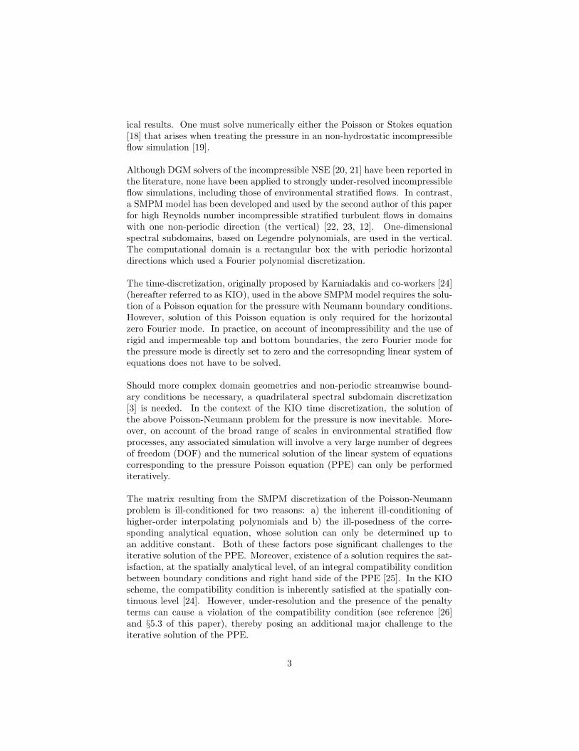
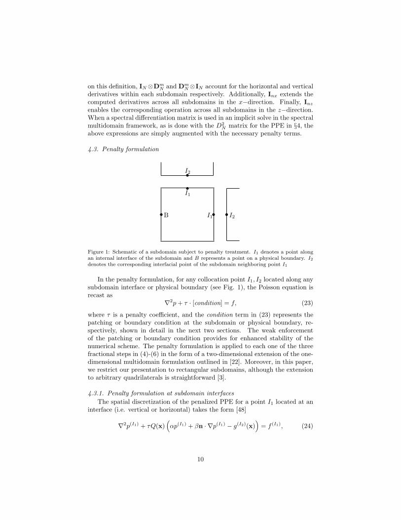
Figure 1: Schematic of a subdomain subject to penalty treatment. I1 denotes a point alongan internal interface of the subdomain and B represents a point on a physical boundary. I2denotes the corresponding interfacial point of the subdomain neighboring point I1

In the penalty formulation, for any collocation point I1, I2 located along anysubdomain interface or physical boundary (see Fig. 1), the Poisson equation isrecast as

∇2p+ τ · [condition] = f, (23)

where τ is a penalty coefficient, and the condition term in (23) represents thepatching or boundary condition at the subdomain or physical boundary, re-spectively, shown in detail in the next two sections. The weak enforcementof the patching or boundary condition provides for enhanced stability of thenumerical scheme. The penalty formulation is applied to each one of the threefractional steps in (4)-(6) in the form of a two-dimensional extension of the one-dimensional multidomain formulation outlined in [22]. Moreover, in this paper,we restrict our presentation to rectangular subdomains, although the extensionto arbitrary quadrilaterals is straightforward [3].

4.3.1. Penalty formulation at subdomain interfaces

The spatial discretization of the penalized PPE for a point I1 located at aninterface (i.e. vertical or horizontal) takes the form [48]

∇2p(I1) + τQ(x)(

αp(I1) + βn · ∇p(I1) − g(I2)(x))

= f (I1), (24)

10

whereg(I2)(x) = γp(I2) + δn · ∇p(I2). (25)

In this case, the variables α, β, γ, δ are constants of the penalty method, set toone in practice [1, 22], and Q(x) is a Dirac delta function which ensures thatthe patching condition is applied only along the subdomain interfaces.

Expressions and limits for the penalty coefficients are derived based on de-termination of energy bounds in the evolution of the time-dependent linearizedBurgers equation [1]. Following [22] the choice of penalty coefficients for thediffusion equation is found to perform robustly for the PPE. As a result, at thesubdomain interfaces, the penalty coefficient must be chosen within the limits[1, 22, 3]

τ =1

ωεβ

[

ε+ 2κ− 2√

κ2 + εκ] 2

LIx

≤ τ ≤1

ωεβ

[

ε+ 2κ+ 2√

κ2 + εκ] 2

LIx

,

(26)where ω = 2/(N(N − 1)) is a GLL quadrature weight, ε is the correspondingdiffusion coefficient, set to one [48] and κ = ωα/β [1, 48]. For a horizontalinterface I1,

2LI

x

is a mapping coefficient and LIx the length of the subdomain.

For a vertical interface, the subdomain height LIz is used instead. The degree

of enforcement of the patching condition is set by the proximity of the penaltycoefficient to the upper limit of Eq. (26). Our practical experience dictates thata choice of τ positioned closer to the lower limit works robustly for the problemof interest. Finally, there is no special formulation at the subdomain corners,which are treated as standard points along the vertical or horizontal interfaces.

4.3.2. Penalty treatment at physical boundaries

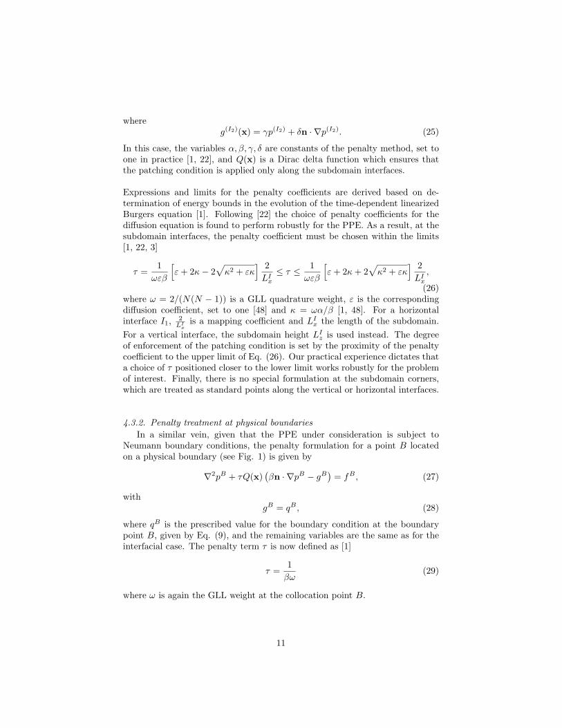
In a similar vein, given that the PPE under consideration is subject toNeumann boundary conditions, the penalty formulation for a point B locatedon a physical boundary (see Fig. 1) is given by

∇2pB + τQ(x)(βn · ∇pB − gB

)= fB , (27)

withgB = qB , (28)

where qB is the prescribed value for the boundary condition at the boundarypoint B, given by Eq. (9), and the remaining variables are the same as for theinterfacial case. The penalty term τ is now defined as [1]

τ =1

βω(29)

where ω is again the GLL weight at the collocation point B.

11

5. Properties of the discrete pressure Poisson equation

5.1. The discrete Poisson pressure equation

Once discretized, the pressure Poisson equation can be written as a linearsystem:

Ax = b, (30)

where the matrix A is the discrete analog of the penalized Laplacian and is con-structed from the tensor product definitions given in Eq. (21)-(22) augmentedwith the contribution of the boundary/patching conditions at the boundaries/interfaces.Additionally, x is the solution vector (i.e. the pressure), and b = ∇ ·

(− v

∆t

)is

the right-hand-side vector which contains information from the convective termand the Neumann boundary conditions (see Eq. (8) -(9)).

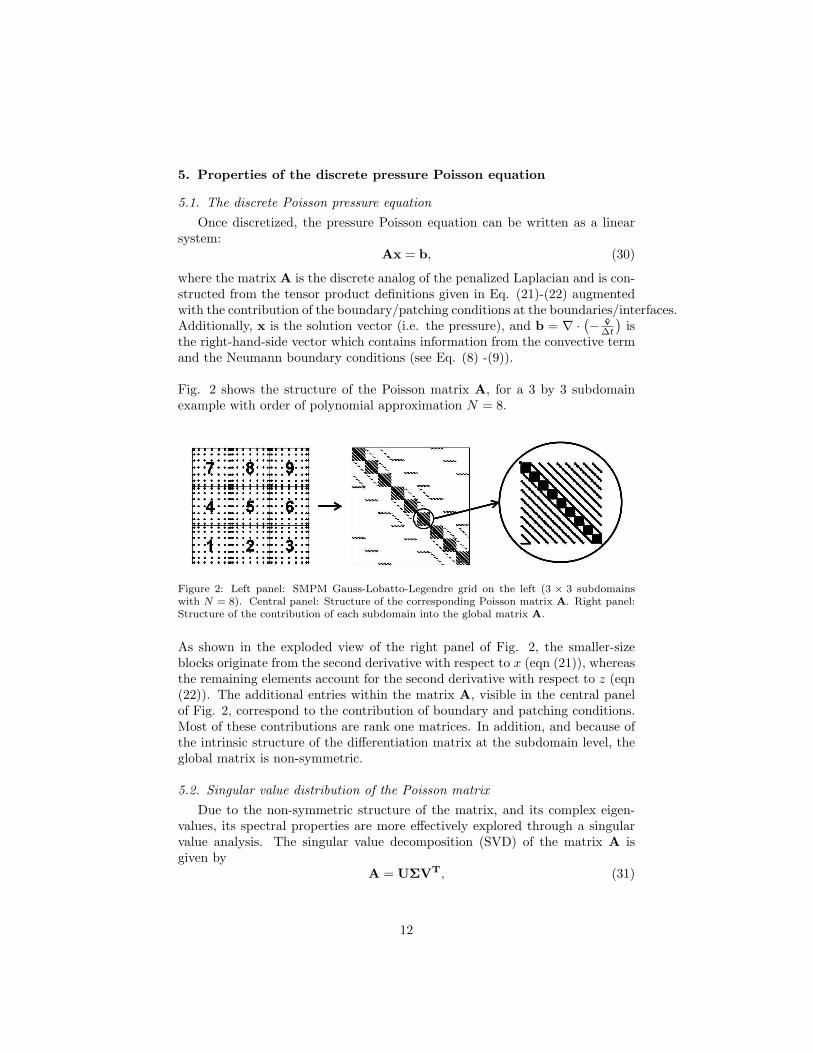
Fig. 2 shows the structure of the Poisson matrix A, for a 3 by 3 subdomainexample with order of polynomial approximation N = 8.

Figure 2: Left panel: SMPM Gauss-Lobatto-Legendre grid on the left (3 × 3 subdomainswith N = 8). Central panel: Structure of the corresponding Poisson matrix A. Right panel:Structure of the contribution of each subdomain into the global matrix A.

As shown in the exploded view of the right panel of Fig. 2, the smaller-sizeblocks originate from the second derivative with respect to x (eqn (21)), whereasthe remaining elements account for the second derivative with respect to z (eqn(22)). The additional entries within the matrix A, visible in the central panelof Fig. 2, correspond to the contribution of boundary and patching conditions.Most of these contributions are rank one matrices. In addition, and because ofthe intrinsic structure of the differentiation matrix at the subdomain level, theglobal matrix is non-symmetric.

5.2. Singular value distribution of the Poisson matrix

Due to the non-symmetric structure of the matrix, and its complex eigen-values, its spectral properties are more effectively explored through a singularvalue analysis. The singular value decomposition (SVD) of the matrix A isgiven by

A = UΣVT, (31)

12

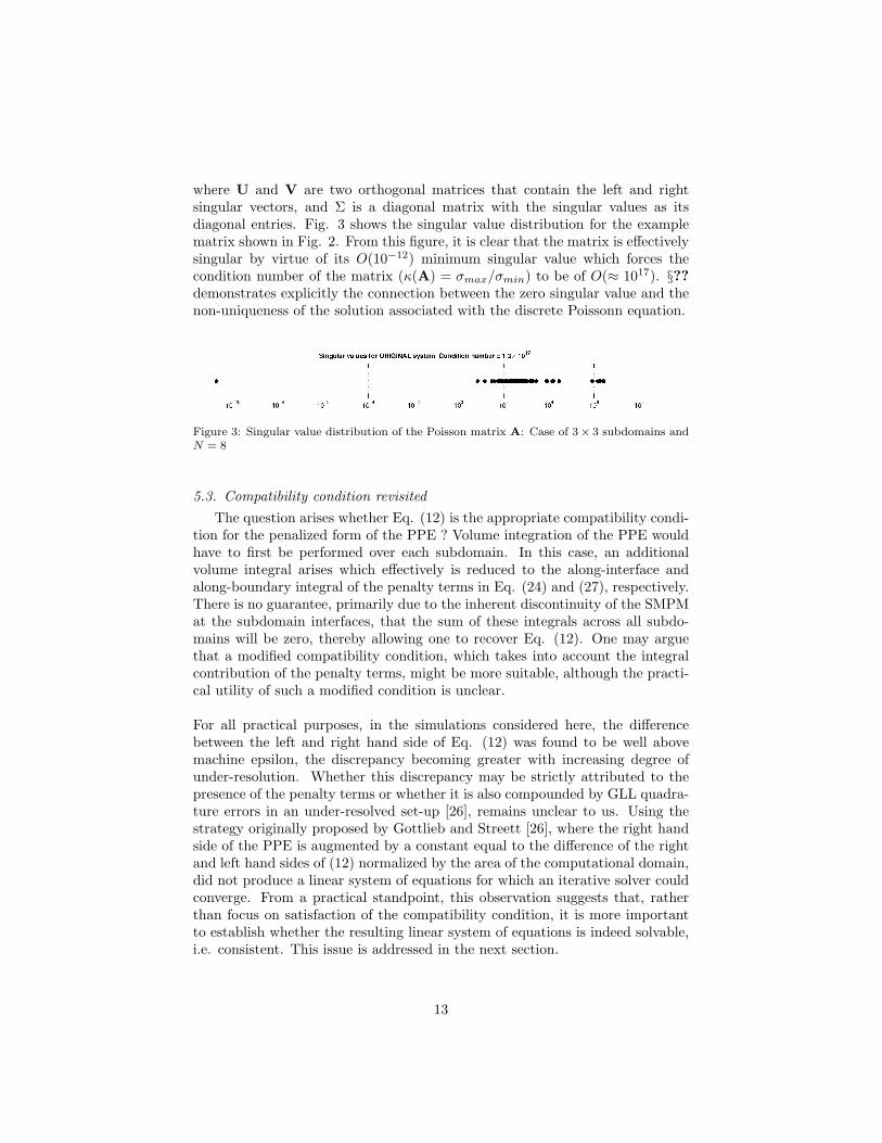
where U and V are two orthogonal matrices that contain the left and rightsingular vectors, and Σ is a diagonal matrix with the singular values as itsdiagonal entries. Fig. 3 shows the singular value distribution for the examplematrix shown in Fig. 2. From this figure, it is clear that the matrix is effectivelysingular by virtue of its O(10−12) minimum singular value which forces thecondition number of the matrix (κ(A) = σmax/σmin) to be of O(≈ 1017). §??demonstrates explicitly the connection between the zero singular value and thenon-uniqueness of the solution associated with the discrete Poissonn equation.

Figure 3: Singular value distribution of the Poisson matrix A: Case of 3× 3 subdomains andN = 8

5.3. Compatibility condition revisited

The question arises whether Eq. (12) is the appropriate compatibility condi-tion for the penalized form of the PPE ? Volume integration of the PPE wouldhave to first be performed over each subdomain. In this case, an additionalvolume integral arises which effectively is reduced to the along-interface andalong-boundary integral of the penalty terms in Eq. (24) and (27), respectively.There is no guarantee, primarily due to the inherent discontinuity of the SMPMat the subdomain interfaces, that the sum of these integrals across all subdo-mains will be zero, thereby allowing one to recover Eq. (12). One may arguethat a modified compatibility condition, which takes into account the integralcontribution of the penalty terms, might be more suitable, although the practi-cal utility of such a modified condition is unclear.

For all practical purposes, in the simulations considered here, the differencebetween the left and right hand side of Eq. (12) was found to be well abovemachine epsilon, the discrepancy becoming greater with increasing degree ofunder-resolution. Whether this discrepancy may be strictly attributed to thepresence of the penalty terms or whether it is also compounded by GLL quadra-ture errors in an under-resolved set-up [26], remains unclear to us. Using thestrategy originally proposed by Gottlieb and Streett [26], where the right handside of the PPE is augmented by a constant equal to the difference of the rightand left hand sides of (12) normalized by the area of the computational domain,did not produce a linear system of equations for which an iterative solver couldconverge. From a practical standpoint, this observation suggests that, ratherthan focus on satisfaction of the compatibility condition, it is more importantto establish whether the resulting linear system of equations is indeed solvable,i.e. consistent. This issue is addressed in the next section.

13

5.4. Consistency of the linear system of equations

The system of equations (30) is consistent if

uT0 Ax = uT

0 b = 0, (32)

where u0 is the left null singular vector of the matrix A [46]. Eq. (32) indicatesthat the PPE has a solution if the forcing vector b is orthogonal to the leftnull singular vector u0. In reference [25], this rationale is outlined for matricesobtained for low-order schemes and real eigenvalues, in the context of an eigen-decomposition of the matrix A and its transpose AT .

In practice the condition (32) is usually not fulfilled, for reasons outlined inthe previous section, and a regularization has to be applied to make the righthand side of (30) orthogonal to the left null singular vector u0 [25], i.e.

Ax = (I− u0uT0 )b = b (33)

where b is the orthogonal complement of b onto u0. Consistency, as representedby Eq. (32), is now ensured to machine epsilon since

uT0 Ax = uT

0 (b− u0uT0 b)

= uT0 b− uT

0 u0uT0 b = 0 (34)

It is important to recall that if the PPE matrix is symmetric a standard eigen-decomposition may be used where there is only one null eigenvector which is aconstant vector [25]. In this case, the implementation of (33) is trivial. However,when the matrix is non-symmetric, as is the case with the SMPM, the left nullsingular vector u0 is no longer constant and has to be explicitly computed. Fora large matrix, typical of environmental flow simulations with many degrees offreedom, the computational cost for a full singular value decomposition (SVD) isprohibitive. As availability of the left null singular vector is of vital importancefor the efficient and robust solution of the SMPM-discretized pressure Poissonequation, an alternative procedure to obtain u0 is presented in §7.

6. Null singular vector removal

The singularity of the Poisson matrix can pose a significant impedimentto the iterative solution of the associated linear system of equations. In thissection, we provide an overview of strategies to remove the null singular vector,including either commonly used ones and also strategies developed specificallyfor the SMPM-discretized Poisson matrix. Note that the former are focused onremoving the constant part of the solution, without necessarily considering asingular value decomposition (or eigendecomposition)of the matrix.

14

6.1. Commonly used strategies

6.1.1. Dirichlet boundary condition at a single point

This widely used technique consists of imposing a Dirichlet condition at onepoint along the physical boundaries [49]. As a result, the indeterminate additiveconstant responsible for a non-unique solution is now set equal to the value givenby the Dirichlet condition. The null singular value is then shifted to the regionwhere the remaining singular values are clustered and the matrix A is no longersingular. Although straightforward in its implementation, when used within theSMPM framework, this technique produces a particularly detrimental spuriouseffect. The insertion of a Dirichlet condition at a point on a boundary otherwisesubject to Neumann conditions, produces a localized spike in the solution. Inan incompressible Navier-Stokes simulation, this spike will grow in magnitudeand pollute the solution in the interior of the computational domain. Note thatthis spurious effect is also observed when the Neumann boundary conditions areenforced strongly.

Furthermore, this technique modifies the tensor product structure of the globalmatrix A. As a result, the efficiency of any preconditioning technique at hand,which is based on the original structure of the matrix, is adversely impacted asthe system solved is no longer equivalent to the original one. Finally, use ofa Dirichlet pressure boundary condition along an entire boundary of the com-putational domain might be dictated by the physics of the actual problem athand, e.g. for an outflow boundary [50]. Such an approach obviously avoidsany singularity issues of the Poisson matrix but is not always feasible since thepressure distribution along a physical boundary is not always known a priori.

6.1.2. Constant part removal

Taking into account that the solution of the system of equations can bedetermined up to an additive constant, an alternative approach to make thesolution unique is by forcing its volume integral (i.e. its mean) to be zero [18]:

∫

Ω

p dΩ = 0. (35)

The discrete analog of Eq. (35) consists of adding one row with the Gauss-Legendre integration weights to the global matrix A and solving the overde-termined system of equations in a least squares sense. We did not pursue thisoption as it is unclear how one may obtain an efficient iterative solution of theresulting normal equations, with concerns of appropriate preconditioner designalso being an issue.

In the same vein, the constraint (35) can be imposed in the form of a penaltyterm, i.e. by solving

∇2p+ τ

∫

Ω

p dp = f , (36)

15

which in matrix form becomes

Ax+ τ1wTx = b (37)

where τ is a penalty coefficient, 1 is a vector of all ones with size equal to thetotal number of degrees of freedom, as well as w that is a vector containingthe Legendre weights for the numerical integration. For the matrix used in thiswork, the numerical results obtained with this techniques were not satisfactorysince the new matrix (A+ 1wT) is dense, which translates into a loss of theblock structure, and an inefficient performance of the preconditioners custom-arily designed for the matrix A.

Alternatively, one can appeal to the SVD of the Poisson matrix to remove theconstant component of the PPE solution at the linear algebra level. Specifically,the solution can be rewritten as

x = (UΣVT)−1b (38)

x =uT0 b

σ0v0 +

N∑

i−1

uTi b

σi

vi, (39)

where ui,vi are the left and right singular vectors of the matrix A, and σi arethe corresponding singular values. Thus, in Eq. (39), the solution is writtenout in the form of an orthogonal expansion where the basis vectors are the rightsingular vectors vi, and the corresponding coefficients are uT

i b/σi. The rightnull vector v0 can readily be shown to have constant entries. Moreover, for aconsistent singular system and exact arithmetic, the coefficient uT

0 b/σ0 is equalto zero divided by zero. Therefore, the first term in (39) corresponds to theconstant part of the solution and is thus the discrete equivalent of the inde-terminate additive constant of the analytical solution to the Poisson-Neumannproblem in (15). In practice, the constant uT

0 b/σ0 is found to have a non-zerovalue which is bounded by machine epsilon at its lower limit, and round offerrors at its upper limit.

Now, at each time step, the constant part of the solution may be removed byforcing the solution vector x to be orthogonal to the right null singular vectorthrough

x = x− v0vT0 x,

where vT0 x is the coefficient of the constant component in the orthogonal ex-

pansion of Eq. (39). The above regularization technique is similar to the oneused to enforce consistency of the linear system of equations (see Eq. (33) ).However, enforcing the orthogonality of the solution to the right null singularvector is effectively a post-processing action, i.e. it is implemented after the so-lution to the PPE has been iteratively computed and does not guarantee moreefficient and robust performance of the iterative solution algorithm. For such aregularization to be implemented in the framework of the actual iterative solu-tion algorithm, such as the conjugate gradient or GMRES methods, one would

16

have to ensure that each new Krylov vector is orthogonal to the right null sin-gular vector. For the conjugate gradient method, the iterative solver of choicefor SEM [18], this strategy works well since each iteration gives an improvedsolution vector, and the final solution is thus orthogonal to the null vector (PaulFischer, personal communication). When the above condition is imposed withinthe GMRES framework, the orthogonality among elements of the Krylov sub-space is adversely impacted. Should a solution exist, the number of iterationsto converge to it will then actually increase significantly. Consequently, moreefficient avenues of ensuring a unique solution for the SMPM-discretized PPEare needed.

6.2. Strategies for the SMPM-discretized Poisson equation

6.2.1. Reduced system via Householder matrices

This approach is based on a combination of the SVD with Householder ma-trices [46]. The main goal is, by exploiting the properties of the associatedorthogonal matrices, to reduce the n × n system of equations to an equivalentreduced one, with a null-space of zero dimension and a rank of n−1. Effectively,the reduced matrix is such that it guides the iterative solution method, GMRESin this case, to operate within a vector space that is orthogonal to the null spaceof A.

To describe the method, let us assume that we have the left and right nullsingular vectors u0 and v0 of the matrix A. For each one of these two vectors,an orthonormal basis P and Q can be built using Householder transformations,

P = I− 2hLh

TL

hTLhL

= [p1,p2, · · · ,pN], (40)

Q = I− 2hRh

TR

hTRhR

= [q1,q2, · · · ,qN], (41)

where hL and hR are the left and right Householder vectors [46], and pi,qi,with i = 1, · · · , n, are the column vectors of the matrices P and Q respectively.It is important to note that, in this construction, p1 = u0 and q1 = v0. Oncethe bases are built, the null vectors u0,v0 can be eliminated from the basis toobtain a reduced set of basis vectors Pr and Qr

P = [u0,p2, · · · ,pN] → Pr = [p2, · · · ,pN], (42)

Q = [v0,q2, · · · ,qN] → Qr = [q2, · · · ,qN]. (43)

Following some algebraic manipulations, the reduced system of Eq. (44) isfinally written as

PTr AQry = PT

r b, , (44)

where y = QTr x. The SVD of the reduced matrix PT

r AQr shows that its sin-gular value distribution is very similar to that of the original matrix A but

17

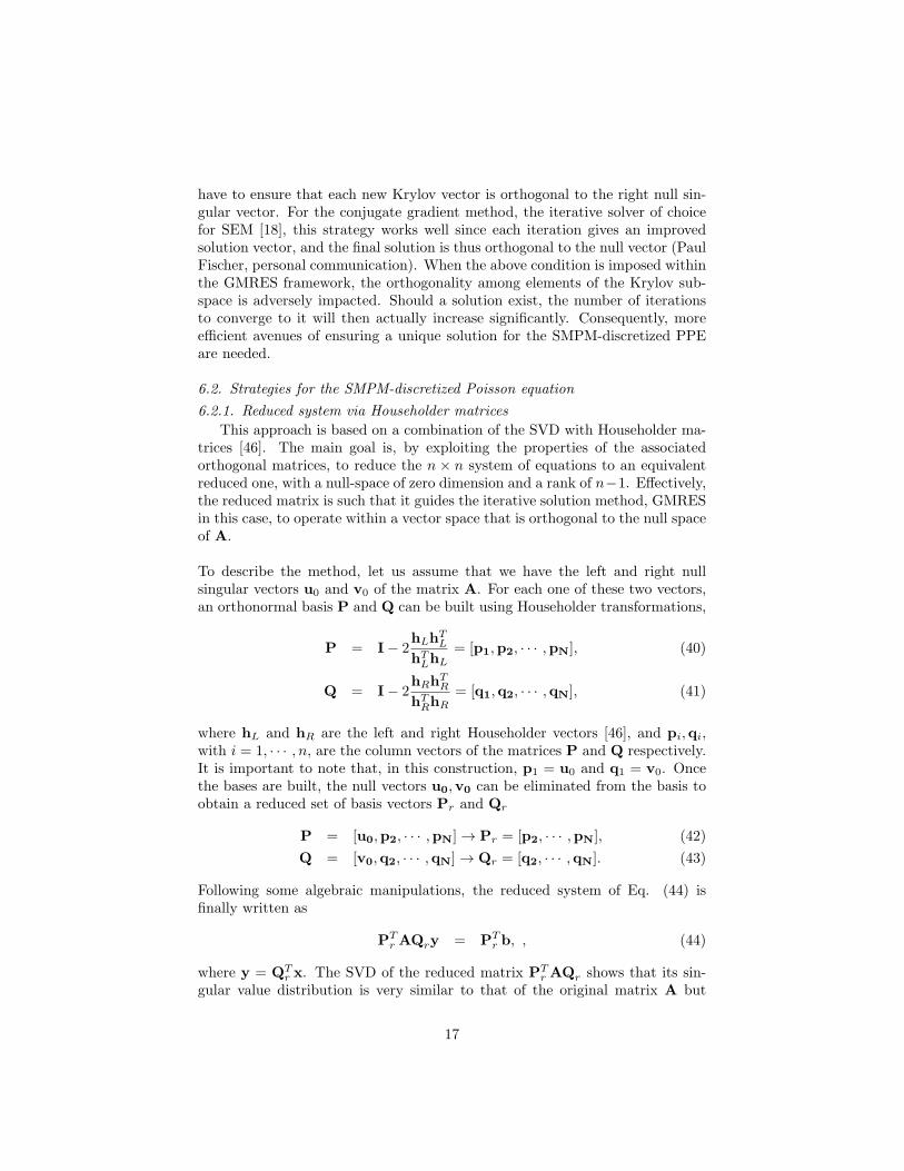
with the main difference that the reduced system is free of the null singularvalue, i.e. the reduced matrix is non-singular. An example of the distribu-tion of singular values for the matrix of the reduced system corresponding to aPoisson-Neumann problem with 3×3 subdomains and N = 8 is shown in Fig. 4.The resulting modified singular value distribution is equivalent to eliminatingthe term uT

0 b/σ0 from Eq. (39), which translates into a unique solution forthe system of equations and a significantly lower condition number for the newmatrix PT

r AQr.

Figure 4: Singular value distribution of the matrix URAVT

R, where A is the matrix of Fig.

3, obtained with the reduced system technique via Householder matrices. Unlike Fig. 3, thenull singular value σ0 is now absent.

Given that (QTr )

−1 = Qr, the final solution to the system of equations is com-puted as

x = Qry (45)

Note that none of the matrices used in this method are explicitly built andno direct matrix-matrix multiplications are involved. The final solution is con-structed through a sequence of matrix-vector multiplications, which are implicitin the solution of a linear system of equations with a Krylov subspace method,such as GMRES.

6.2.2. Augmented system via bordered systems

An alternative approach is based on the concept of augmented (bordered)systems [51]. In this case, the augmented system of equations is expressed as

(A d

cT 0

)(x

α

)

=

(b

g

)

(46)

where c and d are two vectors of dimension n that satisfy the following condi-tions

dTu0 6= 0 (47)

cTv0 6= 0 (48)

By expanding Eq. (46) we obtain

Ax+ αd = b (49)

cTx = 0 (50)

18

If Eq. (49) is multiplied by uT0 the only way in which the system is consistent

is for α = 0uT0 Ax+ αuT

0 d = uT0 b (51)

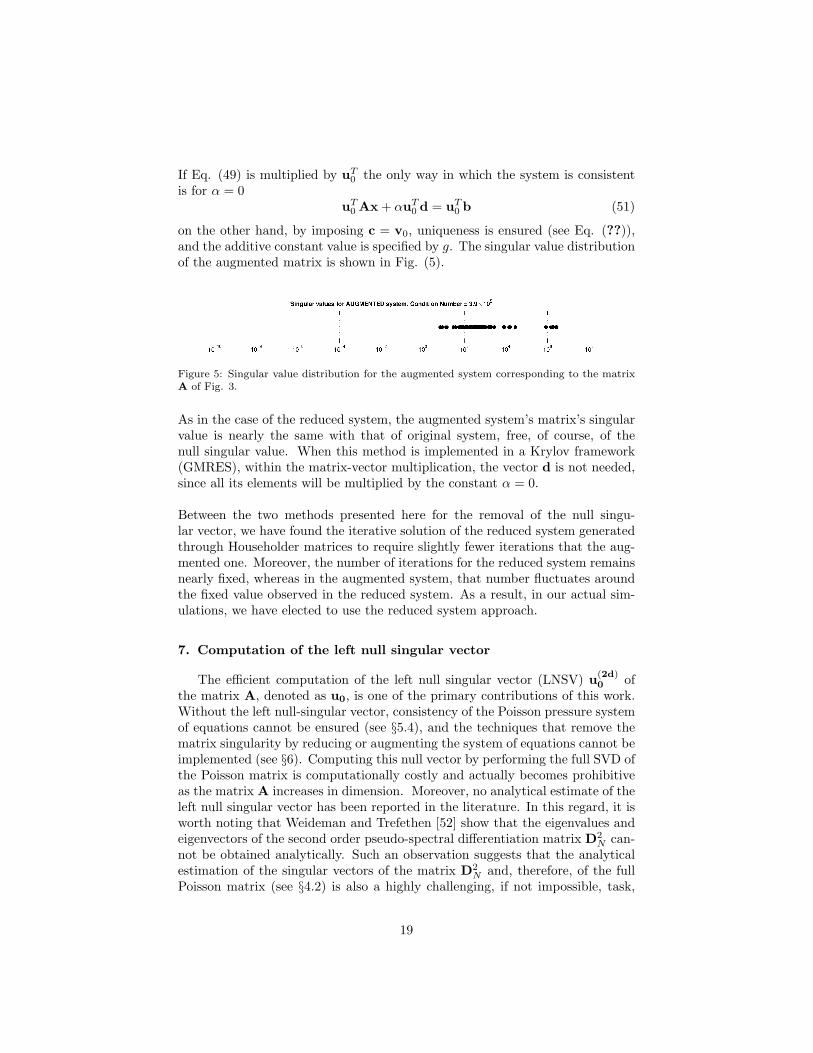
on the other hand, by imposing c = v0, uniqueness is ensured (see Eq. (??)),and the additive constant value is specified by g. The singular value distributionof the augmented matrix is shown in Fig. (5).

Figure 5: Singular value distribution for the augmented system corresponding to the matrixA of Fig. 3.

As in the case of the reduced system, the augmented system’s matrix’s singularvalue is nearly the same with that of original system, free, of course, of thenull singular value. When this method is implemented in a Krylov framework(GMRES), within the matrix-vector multiplication, the vector d is not needed,since all its elements will be multiplied by the constant α = 0.

Between the two methods presented here for the removal of the null singu-lar vector, we have found the iterative solution of the reduced system generatedthrough Householder matrices to require slightly fewer iterations that the aug-mented one. Moreover, the number of iterations for the reduced system remainsnearly fixed, whereas in the augmented system, that number fluctuates aroundthe fixed value observed in the reduced system. As a result, in our actual sim-ulations, we have elected to use the reduced system approach.

7. Computation of the left null singular vector

The efficient computation of the left null singular vector (LNSV) u(2d)0 of

the matrix A, denoted as u0, is one of the primary contributions of this work.Without the left null-singular vector, consistency of the Poisson pressure systemof equations cannot be ensured (see §5.4), and the techniques that remove thematrix singularity by reducing or augmenting the system of equations cannot beimplemented (see §6). Computing this null vector by performing the full SVD ofthe Poisson matrix is computationally costly and actually becomes prohibitiveas the matrix A increases in dimension. Moreover, no analytical estimate of theleft null singular vector has been reported in the literature. In this regard, it isworth noting that Weideman and Trefethen [52] show that the eigenvalues andeigenvectors of the second order pseudo-spectral differentiation matrix D2

N can-not be obtained analytically. Such an observation suggests that the analyticalestimation of the singular vectors of the matrix D2

N and, therefore, of the fullPoisson matrix (see §4.2) is also a highly challenging, if not impossible, task,

19

which is outside of the scope of this paper.

We instead resort to an alternative approach, whose main idea consists of usingthe Kronecker (tensor) product properties of the spectral multidomain methodsto extend concepts from one-dimensional domains to two-dimensional domains(see §4.2). This approach is validated by an experimental proof where the LNSVcomputed via Kronecker products is compared with the corresponding one com-puted with the MATLAB built-in function svds.

7.1. Doubly-periodic domain

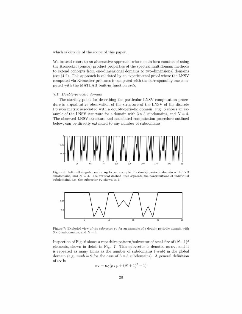
The starting point for describing the particular LNSV computation proce-dure is a qualitative observation of the structure of the LNSV of the discretePoisson matrix associated with a doubly-periodic domain. Fig. 6 shows an ex-ample of the LNSV structure for a domain with 3× 3 subdomains, and N = 4.The observed LNSV structure and associated computation procedure outlinedbelow, can be directly extended to any number of subdomains.

25 50 75 100 125 150 175 200 225

−0.1

−0.05

0

Figure 6: Left null singular vector u0 for an example of a doubly periodic domain with 3× 3subdomains, and N = 4. The vertical dashed lines separate the contributions of individualsubdomains, i.e. the subvector sv shown in 7.

5 10 15 20 25

−0.1

−0.05

0

Figure 7: Exploded view of the subvector sv for an example of a doubly periodic domain with3× 3 subdomains, and N = 4.

Inspection of Fig. 6 shows a repetitive pattern/subvector of total size of (N+1)2

elements, shown in detail in Fig. 7. This subvector is denoted as sv, and itis repeated as many times as the number of subdomains (nsub) in the globaldomain (e.g. nsub = 9 for the case of 3 × 3 subdomains). A general definitionof sv is

sv = u0(p : p+ (N + 1)2 − 1)

20

with p = 1 + (j − 1)(N + 1)2, where j = 1, . . . , nsub represents the j-th subdo-main. Based on this definition and our visual observations, we have found that,for the case of uniform-sized subdomains, we can construct the LNSV u0 as

u0 =1nsub ⊗ sv

‖1nsub ⊗ sv‖2(52)

where 1nsub is a vector of ones with nsub elements. For the more general case ofsubdomains with different dimensions, observation indicates that the magnitudeof the elements of sv scales with the area of the particular subdomain it origi-nates from. For a doubly-periodic domain, with any number of arbitrarily-sizedsubdomains, the global LNSV is then generally computed as

u0 =a⊗ sv

‖a⊗ sv‖2(53)

where a is a vector of nsub elements, which contains the area of each subdomain.

1 2 3 4 5−0.4

−0.3

−0.2

−0.1

0

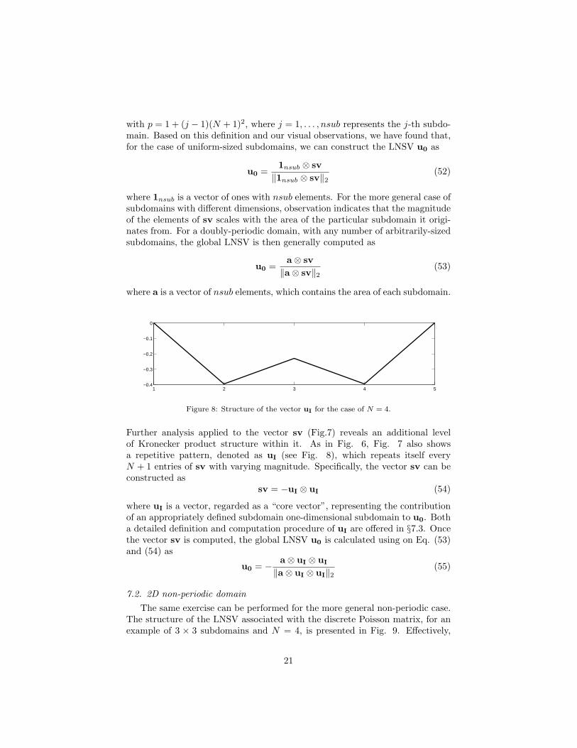
Figure 8: Structure of the vector uI for the case of N = 4.

Further analysis applied to the vector sv (Fig.7) reveals an additional levelof Kronecker product structure within it. As in Fig. 6, Fig. 7 also showsa repetitive pattern, denoted as uI (see Fig. 8), which repeats itself everyN + 1 entries of sv with varying magnitude. Specifically, the vector sv can beconstructed as

sv = −uI ⊗ uI (54)

where uI is a vector, regarded as a “core vector”, representing the contributionof an appropriately defined subdomain one-dimensional subdomain to u0. Botha detailed definition and computation procedure of uI are offered in §7.3. Oncethe vector sv is computed, the global LNSV u0 is calculated using on Eq. (53)and (54) as

u0 = −a⊗ uI ⊗ uI

‖a⊗ uI ⊗ uI‖2(55)

7.2. 2D non-periodic domain

The same exercise can be performed for the more general non-periodic case.The structure of the LNSV associated with the discrete Poisson matrix, for anexample of 3 × 3 subdomains and N = 4, is presented in Fig. 9. Effectively,

21

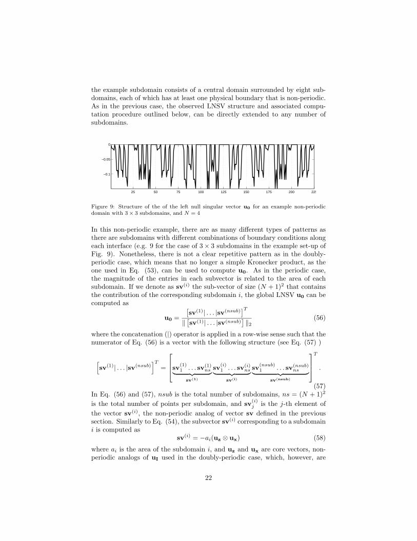
the example subdomain consists of a central domain surrounded by eight sub-domains, each of which has at least one physical boundary that is non-periodic.As in the previous case, the observed LNSV structure and associated compu-tation procedure outlined below, can be directly extended to any number ofsubdomains.

25 50 75 100 125 150 175 200 225

−0.1

−0.05

0

Figure 9: Structure of the of the left null singular vector u0 for an example non-periodicdomain with 3× 3 subdomains, and N = 4

In this non-periodic example, there are as many different types of patterns asthere are subdomains with different combinations of boundary conditions alongeach interface (e.g. 9 for the case of 3× 3 subdomains in the example set-up ofFig. 9). Nonetheless, there is not a clear repetitive pattern as in the doubly-periodic case, which means that no longer a simple Kronecker product, as theone used in Eq. (53), can be used to compute u0. As in the periodic case,the magnitude of the entries in each subvector is related to the area of eachsubdomain. If we denote as sv(i) the sub-vector of size (N + 1)2 that containsthe contribution of the corresponding subdomain i, the global LNSV u0 can becomputed as

u0 =

[sv(1)| . . . |sv(nsub)

]T

‖[sv(1)| . . . |sv(nsub)

]‖2

(56)

where the concatenation (|) operator is applied in a row-wise sense such that thenumerator of Eq. (56) is a vector with the following structure (see Eq. (57) )

[

sv(1)| . . . |sv(nsub)]T

=

sv

(1)1 . . . sv(1)

ns︸ ︷︷ ︸

sv(1)

sv(i)1 . . . sv(i)

ns︸ ︷︷ ︸

sv(i)

sv(nsub)1 . . . sv(nsub)

ns︸ ︷︷ ︸

sv(nsub)

T

.

(57)In Eq. (56) and (57), nsub is the total number of subdomains, ns = (N + 1)2

is the total number of points per subdomain, and sv(i)j is the j-th element of

the vector sv(i), the non-periodic analog of vector sv defined in the previoussection. Similarly to Eq. (54), the subvector sv(i) corresponding to a subdomaini is computed as

sv(i) = −ai(uz ⊗ ux) (58)

where ai is the area of the subdomain i, and uz and ux are core vectors, non-periodic analogs of uI used in the doubly-periodic case, which, however, are

22

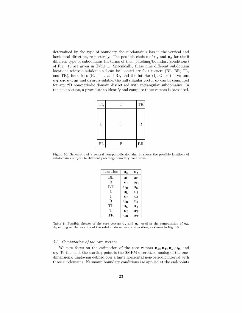
determined by the type of boundary the subdomain i has in the vertical andhorizontal direction, respectively. The possible choices of uz and ux for the 9different type of subdomains (in terms of their patching/boundary conditions)of Fig. 10 are given in Table 1. Specifically, these nine different subdomainlocations where a subdomain i can be located are four corners (BL, BR, TL,and TR), four sides (B, T, L, and R), and the interior (I). Once the vectorsuB,uT,uL,uR and uI are available, the null singular vector u0 can be computedfor any 2D non-periodic domain discretized with rectangular subdomains. Inthe next section, a procedure to identify and compute these vectors is presented.

BL B BR

L I R

TL T TR

Figure 10: Schematic of a general non-periodic domain. It shows the possible locations ofsubdomain i subject to different patching/boundary conditions.

Location ux uz

BL uL uB

B uI uB

BT uR uB

L uL uI

I uI uI

R uR uI

TL uL uT

T uI uT

TR uR uT

Table 1: Possible choices of the core vectors ux and uz, used in the computation of u0,depending on the location of the subdomain under consideration, as shown in Fig. 10

7.3. Computation of the core vectors

We now focus on the estimation of the core vectors uB,uT,uL,uR anduI. To this end, the starting point is the SMPM-discretized analog of the one-dimensional Laplacian defined over a finite horizontal non-periodic interval withthree subdomains. Neumann boundary conditions are applied at the end-points

23

of the full domain, and each subdomain has N + 1 collocation points.

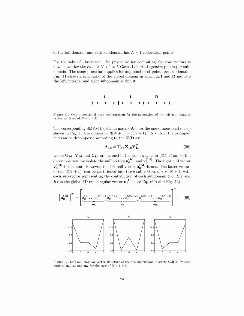
For the sake of illustration, the procedure for computing the core vectors isnow shown for the case of N + 1 = 5 Gauss-Lobatto-Legendre points per sub-domain. The same procedure applies for any number of points per subdomain.Fig. 11 shows a schematic of the global domain in which L, I and R indicatethe left, internal and right subdomain within it.

IL R

Figure 11: One dimensional base configuration for the generation of the left null singularvector u0 (case of N + 1 = 5).

The corresponding SMPM Laplacian matrix A1d for the one-dimensional set-upshown in Fig. 11 has dimension 3(N + 1)× 3(N + 1) (15× 15 in the example)and can be decomposed according to the SVD as:

A1d = U1dΣ1dVT1d (59)

where U1d, V1d and Σ1d are defined in the same way as in (31). From such a

decomposition, we isolate the null vectors u(1d)0 and v

(1d)0 . The right null vector

v(1d)0 is constant. However, the left null vector u

(1d)0 is not. The latter vector,

of size 3(N + 1), can be partitioned into three sub-vectors of size N + 1, witheach sub-vector representing the contribution of each subdomain (i.e. L, I and

R) to the global 1D null singular vector u(1d)0 (see Eq. (60) and Fig. 12)

[

u(1d)0

]T

=

u

(1)0 . . . u

(N+1)0

︸ ︷︷ ︸

uL

u(N+2)0 . . . u

(2N+2)0

︸ ︷︷ ︸

uI

u(2N+3)0 . . . u

(3N+3)0

︸ ︷︷ ︸

uR

T

. (60)

1 2 3 4 5−0.4

−0.3

−0.2

−0.1

0

uL

1 2 3 4 5−0.4

−0.3

−0.2

−0.1

0

uI

1 2 3 4 5−0.4

−0.3

−0.2

−0.1

0

uR

Figure 12: Left null singular vector structure of the one dimensional discrete SMPM Poissonmatrix. uL,uI, and uR for the case of N + 1 = 5

24

In Eq. (60) and Fig. 12, the vectors uL,uI, and uR are the contributions of

the left, central and right subdomains to the global null vector u(1d)0 . Note that

if the same procedure is followed with the canonical 1D subdomains aligned withthe vertical direction, the results are exactly the same as in the horizontal casewith uB = uL and uT = uR. With these considerations, for the case of doubly-periodic domains, the global LNSV is computed strictly through the vector uI

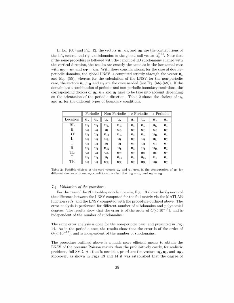
and Eq. (55), whereas for the calculation of the LNSV for the non-periodiccase, the vectors uL,uR and uI are the ones needed (see Eq. (56)-(58)). If thedomain has a combination of periodic and non-periodic boundary conditions, thecorresponding choices of uL,uR and uI have to be take into account dependingon the orientation of the periodic direction. Table 2 shows the choices of ux

and uz for the different types of boundary conditions.

Periodic Non-Periodic x-Periodic z-Periodic

Location ux uz ux uz ux uz ux uz

BL uI uI uL uL uI uL uL uI

B uI uI uI uL uI uL uI uI

BT uI uI uR uL uI uL uR uI

L uI uI uL uI uI uI uL uI

I uI uI uI uI uI uI uI uI

R uI uI uR uI uI uI uR uI

TL uI uI uL uR uI uR uL uI

T uI uI uI uR uI uR uI uI

TR uI uI uR uR uI uR uR uI

Table 2: Possible choices of the core vectors ux and uz used in the computation of u0 fordifferent choices of boundary conditions, recalled that uB = uL and uT = uR

7.4. Validation of the procedure

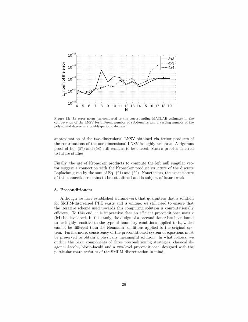
For the case of the 2D doubly-periodic domain, Fig. 13 shows the L2 norm ofthe difference between the LNSV computed for the full matrix via the MATLABfunction svds, and the LNSV computed with the procedure outlined above. Theerror analysis is performed for different number of subdomains and polynomialdegrees. The results show that the error is of the order of O(< 10−12), and isindependent of the number of subdomains.

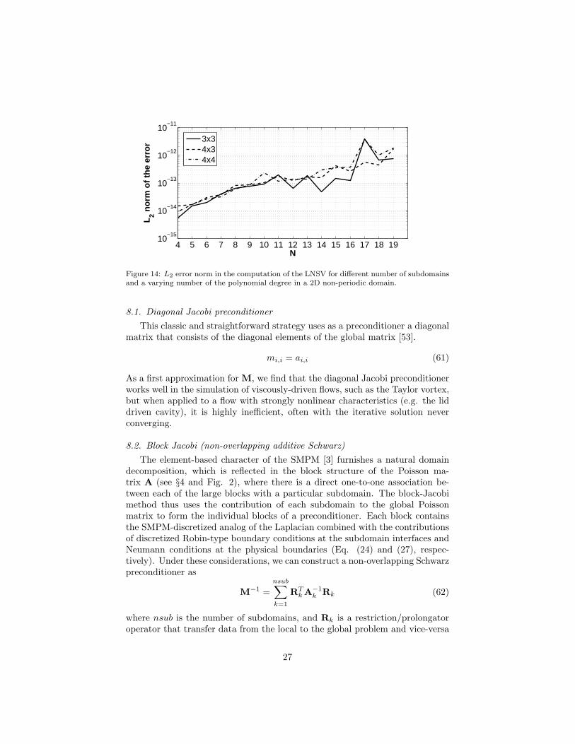
The same error analysis is done for the non-periodic case, and presented in Fig.14. As in the periodic case, the results show that the error is of the order ofO(< 10−12), and is independent of the number of subdomains.

The procedure outlined above is a much more efficient means to obtain theLNSV of the pressure Poisson matrix than the prohibitively costly, for realisticproblems, full SVD. All that is needed a priori are the vectors uL,uI, and uR.Moreover, as shown in Fig.s 13 and 14 it was established that the degree of

25

4 5 6 7 8 9 10 11 12 13 14 15 16 17 18 1910

−15

10−14

10−13

10−12

10−11

N

L2 n

orm

of t

he e

rror

3x34x34x4

Figure 13: L2 error norm (as compared to the corresponding MATLAB estimate) in thecomputation of the LNSV for different number of subdomains and a varying number of thepolynomial degree in a doubly-periodic domain.

approximation of the two-dimensional LNSV obtained via tensor products ofthe contributions of the one-dimensional LNSV is highly accurate. A rigorousproof of Eq. (57) and (58) still remains to be offered. Such a proof is deferredto future studies.

Finally, the use of Kronecker products to compute the left null singular vec-tor suggest a connection with the Kronecker product structure of the discreteLaplacian given by the sum of Eq. (21) and (22). Nonetheless, the exact natureof this connection remains to be established and is subject of future work.

8. Preconditioners

Although we have established a framework that guarantees that a solutionfor SMPM-discretized PPE exists and is unique, we still need to ensure thatthe iterative scheme used towards this computing solution is computationallyefficient. To this end, it is imperative that an efficient preconditioner matrix(M) be developed. In this study, the design of a preconditioner has been foundto be highly sensitive to the type of boundary conditions applied to it, whichcannot be different than the Neumann conditions applied to the original sys-tem. Furthermore, consistency of the preconditioned system of equations mustbe preserved to obtain a physically meaningful solution. In what follows, weoutline the basic components of three preconditioning strategies, classical di-agonal Jacobi, block-Jacobi and a two-level preconditioner, designed with theparticular characteristics of the SMPM discretization in mind.

26

4 5 6 7 8 9 10 11 12 13 14 15 16 17 18 1910

−15

10−14

10−13

10−12

10−11

N

L2 n

orm

of t

he e

rror

3x34x34x4

Figure 14: L2 error norm in the computation of the LNSV for different number of subdomainsand a varying number of the polynomial degree in a 2D non-periodic domain.

8.1. Diagonal Jacobi preconditioner

This classic and straightforward strategy uses as a preconditioner a diagonalmatrix that consists of the diagonal elements of the global matrix [53].

mi,i = ai,i (61)

As a first approximation for M, we find that the diagonal Jacobi preconditionerworks well in the simulation of viscously-driven flows, such as the Taylor vortex,but when applied to a flow with strongly nonlinear characteristics (e.g. the liddriven cavity), it is highly inefficient, often with the iterative solution neverconverging.

8.2. Block Jacobi (non-overlapping additive Schwarz)

The element-based character of the SMPM [3] furnishes a natural domaindecomposition, which is reflected in the block structure of the Poisson ma-trix A (see §4 and Fig. 2), where there is a direct one-to-one association be-tween each of the large blocks with a particular subdomain. The block-Jacobimethod thus uses the contribution of each subdomain to the global Poissonmatrix to form the individual blocks of a preconditioner. Each block containsthe SMPM-discretized analog of the Laplacian combined with the contributionsof discretized Robin-type boundary conditions at the subdomain interfaces andNeumann conditions at the physical boundaries (Eq. (24) and (27), respec-tively). Under these considerations, we can construct a non-overlapping Schwarzpreconditioner as

M−1 =

nsub∑

k=1

RTkA

−1k Rk (62)

where nsub is the number of subdomains, and Rk is a restriction/prolongatoroperator that transfer data from the local to the global problem and vice-versa

27

[28]. Due to the type of boundary conditions applied to each subdomain, thelocal stiffness matrix Ak is non-singular and, in the preconditioner setting, itcan be inverted directly via an LU decomposition.

Numerical results (see §9 for more detail) show that this preconditioner reducesthe number of iterations with respect to the absence of a preconditioner or us-ing only diagonal Jacobi. The number of iterations within the GMRES solverare independent of the degree of approximation, i.e., for a small number ofsubdomains, the block-Jacobi preconditioner deals efficiently with p-refinement.However, when h-refinement is applied, corresponding to a sizable increase innumber of subdomains and degrees of freedom, the number of iterations of theGMRES and computational time of the solver increases linearly (see Fig. 19).Thus, this preconditioner is unsuitable for large problems, such as those encoun-tered in environmental fluid mechanics applications. For such problems, a moreefficient preconditioning strategy is needed.

8.3. Two-Level preconditioner

The implementation of this preconditioner draws from the previous work ofFischer and collaborators [27, 28] and the need for h−scalability. It combines theabove block-Jacobi method as a preconditioner at the fine-level with a coarse-grid component based on a low-order N = 1 SMPM approximation of thePoisson-Neumann problem. The general form of this preconditioner is

M−1 = RT0 A

−10 R0 +

nsub∑

k=1

RTkA

−1k Rk (63)

Eq. (63) is effectively Eq. (62) augmented by the additional term RT0 A

−10 R0

that accounts for the coarse grid correction. R0 is an interpolation matrix [54]that projects a scalar field across different Gauss-Lobatto-Legendre grids andA0 represents the low-order (coarse-level) analog of the Poisson matrix.

As mentioned in the previous section, the solution of the fine level precondi-tioner (Block-Jacobi / Additive Schwarz) does not suffer from the problems ofa nearly singular system due to the Robin type boundary conditions appliedto the subdomain interfaces, which make each one of the blocks non-singular.This is not the case for the coarse grid preconditioner, where the same problemsassociated with the global Poisson matrix once again must be addressed. Inthis regard, a regularization along the lines of Eq. (33) has to be applied to thecoarse-system solver in order to make it consistent, otherwise the preconditionercannot be solved for. As with the block-Jacobi preconditioner, the solution ofthe coarse grid preconditioner is performed with a direct LU solver. In section§9, the scalability of the two-level preconditioner is compared to that of theadditive Schwarz (Block-Jacobi), and diagonal Jacobi.

28

9. Numerical results

9.1. Taylor vortex

This is the first of two test cases used to assess the performance of the pre-viously outlined iterative solution strategies for the Poisson-Neumann problemwithin the framework of an incompressible Navier-Stokes equation solver. Theflow field initially consists of a periodic array of vortices whose velocity fielddiffuses out with time. Periodic boundary conditions are imposed in both direc-tions. The initial condition is based on the analytical solution [20, 5] obtainedfor (x, y) ∈ [−1, 1]2:

u(t, x, y) = − cos(πx) sin(πy) exp

(−2π2t

Re

)

(64)

w(t, x, y) = sin(πx) cos(πy) exp

(−2π2t

Re

)

(65)

p(t, x, y) = −cos(2πx) + cos(2πy)

4exp

(−4π2t

Re

)

(66)

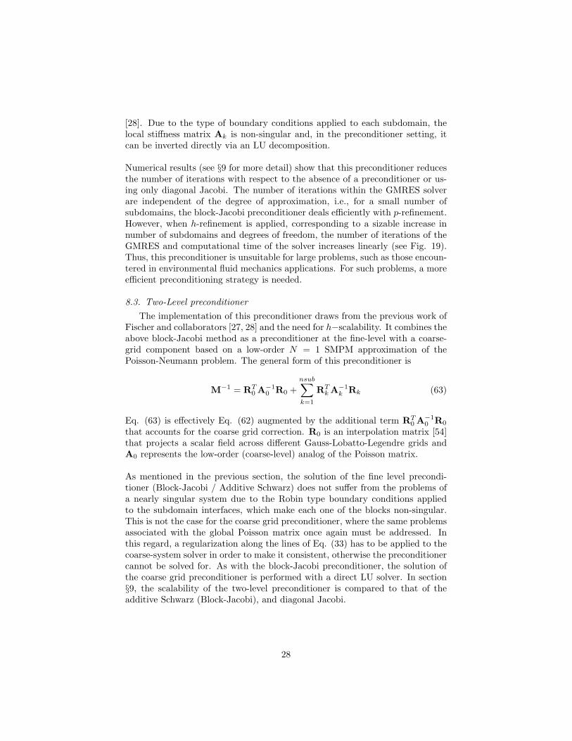
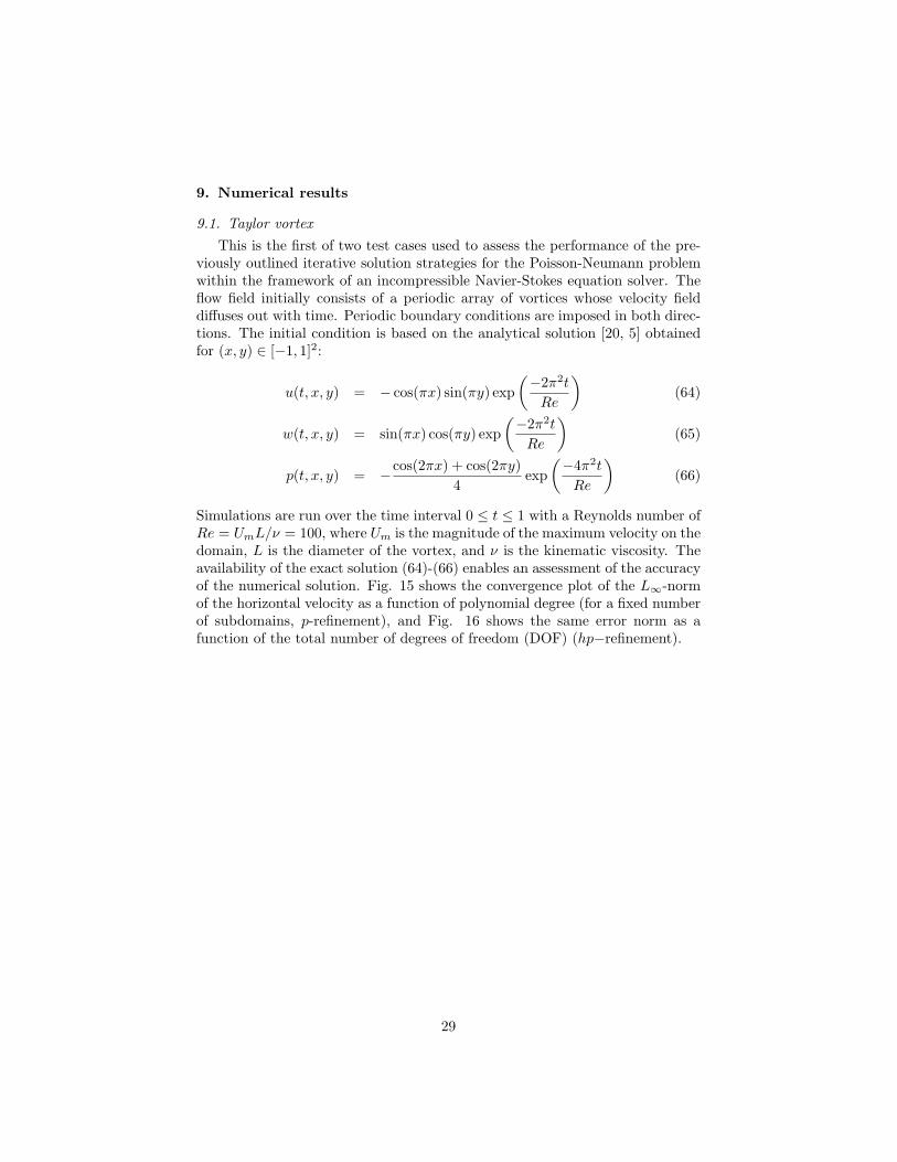
Simulations are run over the time interval 0 ≤ t ≤ 1 with a Reynolds number ofRe = UmL/ν = 100, where Um is the magnitude of the maximum velocity on thedomain, L is the diameter of the vortex, and ν is the kinematic viscosity. Theavailability of the exact solution (64)-(66) enables an assessment of the accuracyof the numerical solution. Fig. 15 shows the convergence plot of the L∞-normof the horizontal velocity as a function of polynomial degree (for a fixed numberof subdomains, p-refinement), and Fig. 16 shows the same error norm as afunction of the total number of degrees of freedom (DOF) (hp−refinement).

29

4 6 8 10 12 14 1610

−5

10−4

10−3

10−2

10−1

100

N

L∞ n

orm

of e

rror

in u

−vel

ocity

Figure 15: L∞-norm of the horizontal velocity for various polynomial degrees and a fixednumber (3× 3 in this particular case)of subdomains. The solid line represents a least-squaresexponential best-fit.

104

105

10−7

10−6

10−5

Degrees of Freedom

L∞ n

orm

of e

rror

in u

−vel

ocity

Figure 16: L∞-norm of the horizontal velocity for a varying number of total degrees orfreedom (obtained through hp−refinement) for the Taylor Vortex problem at three differentvalues of total number of subdomains. Square symbols represent 5× 5 subdomains, triangles10 × 10 subdomains, and circles 15 × 15 subdomains. For each particular number of totalsubdomains, open symbols represents N = 10, and filled symbols N = 14. The solid linerepresents a least-squares power-law best-fit.

The impact of the above discussed preconditioners on the efficiency of the

30

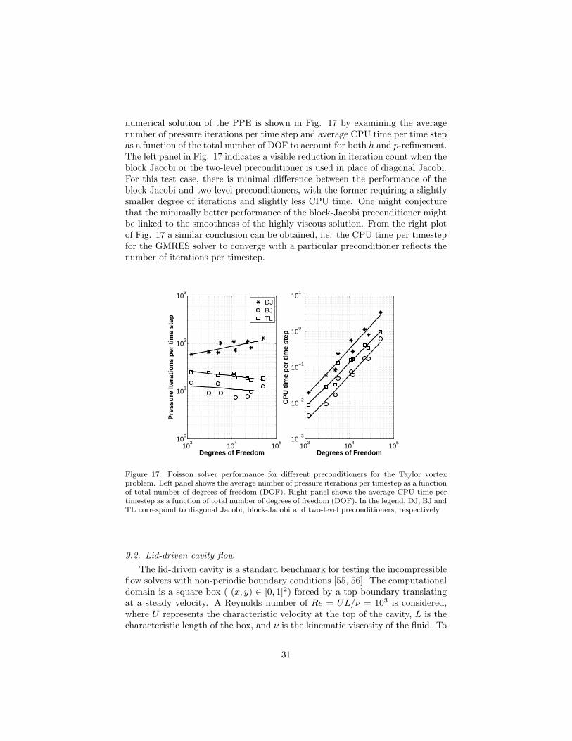
numerical solution of the PPE is shown in Fig. 17 by examining the averagenumber of pressure iterations per time step and average CPU time per time stepas a function of the total number of DOF to account for both h and p-refinement.The left panel in Fig. 17 indicates a visible reduction in iteration count when theblock Jacobi or the two-level preconditioner is used in place of diagonal Jacobi.For this test case, there is minimal difference between the performance of theblock-Jacobi and two-level preconditioners, with the former requiring a slightlysmaller degree of iterations and slightly less CPU time. One might conjecturethat the minimally better performance of the block-Jacobi preconditioner mightbe linked to the smoothness of the highly viscous solution. From the right plotof Fig. 17 a similar conclusion can be obtained, i.e. the CPU time per timestepfor the GMRES solver to converge with a particular preconditioner reflects thenumber of iterations per timestep.

103

104

105

100

101

102

103

Degrees of Freedom

Pre

ssur

e Ite

ratio

ns p

er ti

me

step

103

104

105

10−3

10−2

10−1

100

101

Degrees of Freedom

CP

U ti

me

per

time

step

DJBJTL

Figure 17: Poisson solver performance for different preconditioners for the Taylor vortexproblem. Left panel shows the average number of pressure iterations per timestep as a functionof total number of degrees of freedom (DOF). Right panel shows the average CPU time pertimestep as a function of total number of degrees of freedom (DOF). In the legend, DJ, BJ andTL correspond to diagonal Jacobi, block-Jacobi and two-level preconditioners, respectively.

9.2. Lid-driven cavity flow

The lid-driven cavity is a standard benchmark for testing the incompressibleflow solvers with non-periodic boundary conditions [55, 56]. The computationaldomain is a square box ( (x, y) ∈ [0, 1]2) forced by a top boundary translatingat a steady velocity. A Reynolds number of Re = UL/ν = 103 is considered,where U represents the characteristic velocity at the top of the cavity, L is thecharacteristic length of the box, and ν is the kinematic viscosity of the fluid. To

31

avoid the singularities that arise at the top corners due to discontinuities in theu velocity [55, 57], we consider a modified lid-driven cavity [39], where the topboundary condition is given by

u(x, 1) = −16x2(1− x2

)(67)

v(x, 1) = 0 (68)

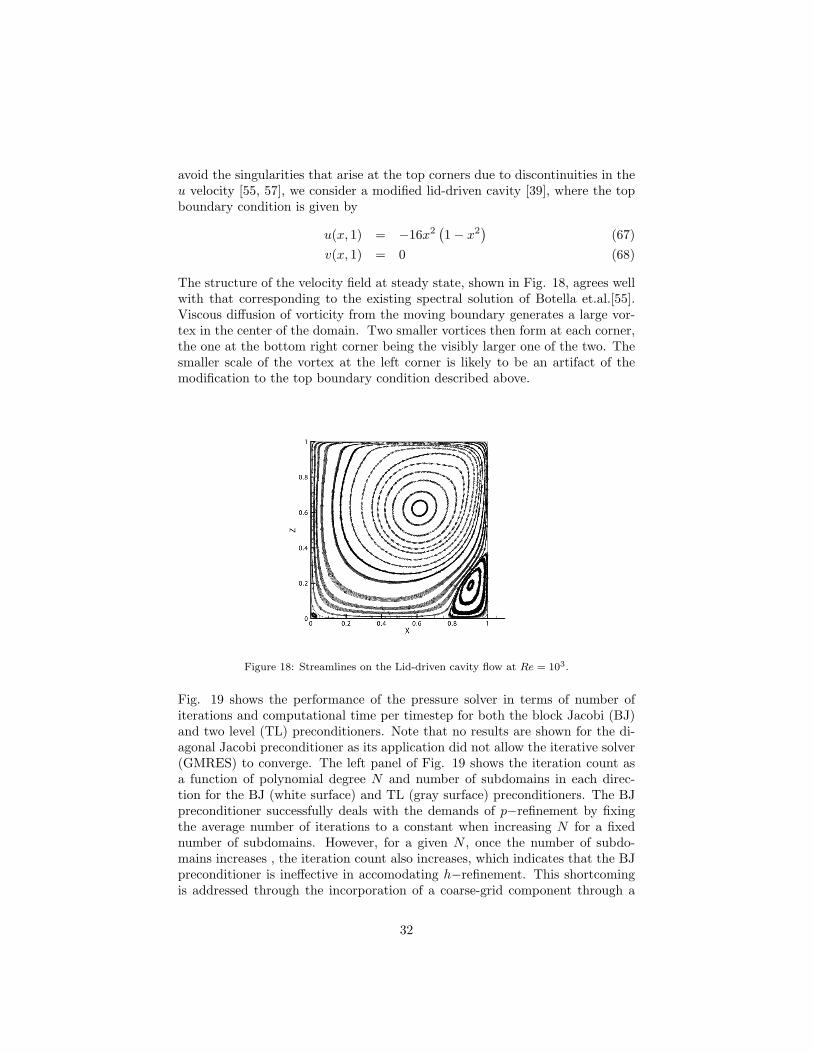
The structure of the velocity field at steady state, shown in Fig. 18, agrees wellwith that corresponding to the existing spectral solution of Botella et.al.[55].Viscous diffusion of vorticity from the moving boundary generates a large vor-tex in the center of the domain. Two smaller vortices then form at each corner,the one at the bottom right corner being the visibly larger one of the two. Thesmaller scale of the vortex at the left corner is likely to be an artifact of themodification to the top boundary condition described above.

Figure 18: Streamlines on the Lid-driven cavity flow at Re = 103.

Fig. 19 shows the performance of the pressure solver in terms of number ofiterations and computational time per timestep for both the block Jacobi (BJ)and two level (TL) preconditioners. Note that no results are shown for the di-agonal Jacobi preconditioner as its application did not allow the iterative solver(GMRES) to converge. The left panel of Fig. 19 shows the iteration count asa function of polynomial degree N and number of subdomains in each direc-tion for the BJ (white surface) and TL (gray surface) preconditioners. The BJpreconditioner successfully deals with the demands of p−refinement by fixingthe average number of iterations to a constant when increasing N for a fixednumber of subdomains. However, for a given N , once the number of subdo-mains increases , the iteration count also increases, which indicates that the BJpreconditioner is ineffective in accomodating h−refinement. This shortcomingis addressed through the incorporation of a coarse-grid component through a

32

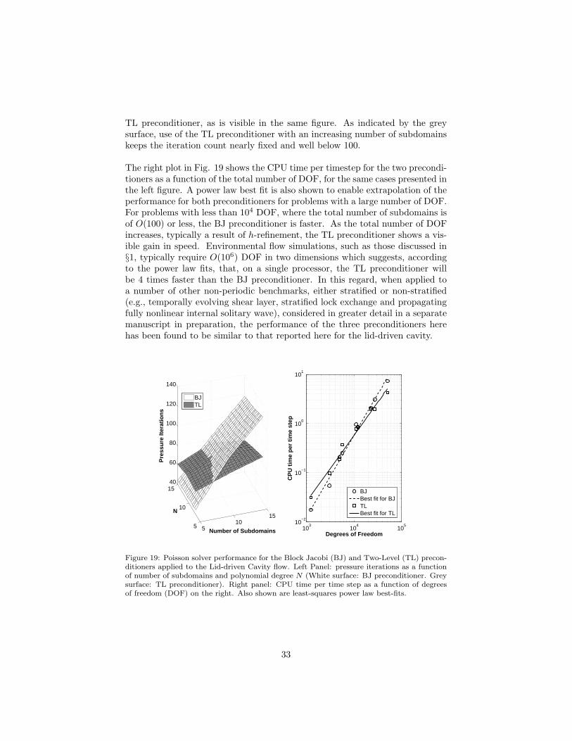
TL preconditioner, as is visible in the same figure. As indicated by the greysurface, use of the TL preconditioner with an increasing number of subdomainskeeps the iteration count nearly fixed and well below 100.

The right plot in Fig. 19 shows the CPU time per timestep for the two precondi-tioners as a function of the total number of DOF, for the same cases presented inthe left figure. A power law best fit is also shown to enable extrapolation of theperformance for both preconditioners for problems with a large number of DOF.For problems with less than 104 DOF, where the total number of subdomains isof O(100) or less, the BJ preconditioner is faster. As the total number of DOFincreases, typically a result of h-refinement, the TL preconditioner shows a vis-ible gain in speed. Environmental flow simulations, such as those discussed in§1, typically require O(106) DOF in two dimensions which suggests, accordingto the power law fits, that, on a single processor, the TL preconditioner willbe 4 times faster than the BJ preconditioner. In this regard, when applied toa number of other non-periodic benchmarks, either stratified or non-stratified(e.g., temporally evolving shear layer, stratified lock exchange and propagatingfully nonlinear internal solitary wave), considered in greater detail in a separatemanuscript in preparation, the performance of the three preconditioners herehas been found to be similar to that reported here for the lid-driven cavity.

510

15

5

10

1540

60

80

100

120

140

Number of Subdomains

N

Pre

ssur

e Ite

ratio

ns

103

104

105

10−2

10−1

100

101

Degrees of Freedom

CP

U ti

me

per

time

step

BJTL

BJBest fit for BJTLBest fit for TL

Figure 19: Poisson solver performance for the Block Jacobi (BJ) and Two-Level (TL) precon-ditioners applied to the Lid-driven Cavity flow. Left Panel: pressure iterations as a functionof number of subdomains and polynomial degree N (White surface: BJ preconditioner. Greysurface: TL preconditioner). Right panel: CPU time per time step as a function of degreesof freedom (DOF) on the right. Also shown are least-squares power law best-fits.

33

10. Discussion

Various preconditioners previously developed for other high-order elementbased methods have been applied to our SMPM-discretized PPE. However,the efficient performance of such pre-existing preconditioners has been foundto be impeded by the discontinuous formulation of SMPM at the subdomain-interfaces, the requirement of Neumann boundary conditions and the non-symmetry of the global Poisson matrix. First, the incomplete LU (ILU) precon-ditioner [53] was examined, which was found to be impractical for large problemsas matrix storage is required. A subsequent step involved a preconditioner basedon the finite difference (FD) discretization of the Laplacian operator [18]. Inthis case, applying the FD discretization at the discontinuous interfaces of theSMPM grid is not a straightforward procedure. As a result, solving the FD pre-conditioner matrix is a costly task, since the resulting matrix is non-symmetricand nearly singular.

A p−multigrid preconditioner has also been tested [58, 35, 59, 60] in orderto take advantage of the hierarchy inherent in the Legendre polynomial basisfunctions used in the SMPM and the fast computation of GLL points and dif-ferentiation matrices. The main problem encountered in this approach is theinefficiency of the smoothing steps which require a significant number of itera-tions (as high as 50) to remove the high frequency oscillations that contaminatethe coarser grid solves encountered at subsequent levels of the multigrid cycle.Finally, a projection technique relying on multiple right hand sides of the PPE,obtained from previous timesteps, [61] was also tested in the framework of aTL-preconditioned GMRES iterative solver, with the puprose of further reduc-ing the total number of iterations. A modified Gram-Schmidt orthogonalizationwas needed instead of the classic Gram-Schmidt for the stable generation ofthe successive right-hand-sides. Unfortunately, unlike what was observed in itsapplication to a conjugate gradient solver used within a SEM framework [61],when applied to the iterative solution of the SMPM-discretized PPE, this tech-nique did not reveal any decrease in iteration count for the GMRES solver.

As a concluding note to this discussion, the coarse-level preconditioner is con-structed using a low-order (N = 1) SMPM discretization of the Laplacian oper-ator. Such a small value of N is chosen to allow for a direct solver (LU factor-ization) to be used for the resulting linear system of equations when computingthe preconditioner. An increase to N = 2 or 3 polynomial could make this LUdecomposition computationally infeasible when the number of subdomains islarge, as is the case of an environmental flow simulation.

11. Summary and concluding remarks

An efficient iterative solution strategy has been developed for the quadrilat-eral spectral multidomain penalty method (SMPM)-discretized pressure Pois-son equation (PPE) with Neumann boundary conditions, implicit in the time-

34

discretization of the two-dimensional incompressible Navier-Stokes equationsthrough a high-order splitting scheme. From the spatially continuous perspec-tive, this system of equations has a solution only if an integral compatibilitycondition involving the right-hand-side of the PPE and the prescribed value ofthe Neumann boundary conditions is fulfilled. However, although the compati-bility condition is automatically satisfied at the spatially continuous (analytical)level in the context of the above splitting scheme, it is unclear whether it is isthe appropriate compability condition for the the SMPM-discretized PPE. Ourobservations further indicate that, in actual incompressible flow simulations,the resuling linear system of equations never satisfy the equivalent solvabilitycondition of orthogonality between the right hand side and the null left singularvector of the Poisson matrix. This lack of solvability may be attributed to thediscontinuity of the pressure solution across subdomains and to inexact quadra-ture, the latter a feature of under-resolved simulations. Finally, the particularboundary conditions give rise to a non-unique solution and, therefore, a near-singular Poisson matrix.

For the resulting linear system of equations, satisfaction of the above solvabilitycondition, i.e. consistency of the linear system of equations, is ensured throughthe regularization that projects the right-hand-side onto the plane orthogonalto the left null singular vector of the global Poisson matrix. Uniqueness of thesolution is ensured at the linear algebra level by reducing the system of equa-tions via Householder matrices or via an augmented matrix technique.

A key contribution of this work is the development of a computationally effi-cient technique to estimate the left null singular vector of the SMPM-discretizedPoisson matrix, which avoids the prohibitively costly SVD of the matrix. Thetwo-dimensional left null singular vector is constructed from its one-dimensionalequivalent which is computed for a canonical one-dimensional SMPM Poissonmatrix defined over three subdomains. Availability of the left null singular vec-tor then enables the above described strategies for ensuring a consistent linearsystem of equations and a unique solution for the PPE.

Even if a consistent linear system of equations and a unique solution are en-sured, the efficient iterative solution of the SMPM-discretized PPE cannot beobtained without an appropriately designed preconditioner. To this end, twopreconditioners, a block Jacobi (BJ), and a two-level preconditioner (TL), havebeen implemented. The performance of both preconditioners has been assessedthrough application to two well-known benchmark problems for the numericalsolution of the incompressible Navier-Stokes equations: the Taylor vortex andthe Lid-driven cavity. The BJ preconditioner is found to prevent the increasein iteration count with increasing p−refinement. However, it cannot provide foran efficient solution at high levels of h−refinement, i.e. an increasing numberof subdomains. For this purpose, a TL preconditioner, a combination of coarse-grid and fine-level approaches has been constructed. Its fine-level component isidentical to the standard BJ preconditioner described above. The coarse-level

35

component of the TL preconditioner is based on a low-order SMPM discretiza-tion and resolves the issue with high-levels of h−refinement. In analogy withthe SMPM-discretized Poisson matrix, the coarse-level component of the TLpreconditioner requires a similar regularization which ensures that the associ-ated linear system is consistent.

Beyond providing a framework solution of the PPE system of equations, thiswork has intended to provide a concentrated overview of the techniques usedby the higher-order method community in the context of the Poisson-Neumannproblem for the pressure field implicit in the numerical solution for the incom-pressible Navier-Stokes equations. In a similar vein, we hope that the techniquesdeveloped here, namely the construction of the left null singular vector and itsapplication to ensuring consistency and a unique solution of the linear systemof equations, will be of interest to the sub-discipline of numerical linear algebrafocused on the iterative solution of consistent singular non-symmetric systems.

Future work can be oriented towards a detailed comparison of the spectral prop-erties of the Poisson-Neumann matrix for different spatial discretizations andconstructing a unified framework for the solution of the nearly-singular sys-tems that arise in the numerical solution of the incompressible Navier-Stokesequations. More efficient preconditioning efforts could focus on exploiting theKronecker product structure of the Poisson matrix, or alternatively, translateto the SMPM the experience gained with algebraic multigrid for continuous anddiscontinuous finite element type methods [62]. Finally, additional considera-tions will arise in the computation (as outlined here) of the left null singularvector for the Poisson matrix resulting from a SMPM discretization of a domainwith deformed, non-square, subdomains.

Acknowledgements

We thank Prof. David Bindel for invaluable advice on the precondition-ing strategies and the iterative solution of nearly-consistent systems. We alsothanks Prof. Luke Olson for the discussions and guidance in the context ofp−multigrid preconditioning. Dr. Paul Fischer is additionally thanked for il-luminating discussions at the 2009 ICOSAHOM conference. The first authoris grateful to Jose Maria Gonzalez Ondina for endless discussions on the sub-tleties of the PPE solver. The first two authors acknowledge the support of NSFCAREER Award OCE 0845558 .

References

[1] J. S. Hesthaven, D. Gottlieb, A stable penalty method for the compress-ible Navier-Stokes equations: I. Open boundary conditions, SIAM J. Sci.Comput. 17 (1996) 579–612.

36

[2] J. S. Hesthaven, A stable penalty method for the compressible Navier-Stokes equations: II. One-dimensional domain decomposition schemes,SIAM J. Sci. Comput. 18 (1997) 658–685.

[3] J. S. Hesthaven, A stable penalty method for the compressible Navier-Stokes equations: III. Multidimensional domain decomposition schemes,SIAM J. Sci. Comput. 20 (1998) 62–93.

[4] J. P. Boyd, Chebyshev and Fourier Spectral Methods, Dover, Mineola, NewYork, 2001.

[5] G. E. Karniadakis, S. Sherwin, Spectral/hp Element Methods for Compu-tational Fluid dynamics, Oxford University Press, 2005.

[6] J. S. Hesthaven, S. Gottlieb, D. Gottlieb, Spectral Methods for Time-Dependent Problems, Cambridge University Press, 2007.

[7] D. A. Kopriva, Implementing Spectral Methods for Partial DifferentialEquations: Algorithms for Engineers and Scientists, Springer Verlag, 2009.

[8] J. S. Hesthaven, T. Warburton, Nodal Discontinuous Galerkin Methods,Springer-Verlag, 2008.

[9] J. A. Escobar-Vargas, P. J. Diamessis, F. X. Giraldo, High-order discon-tinuous element-based schemes for the inviscid shallow water equations:Spectral multidomain penalty and discontinuous Galerkin methods, Appl.Math. Comput. (2011).

[10] S. A. Thorpe, The Turbulent Ocean, Cambridge University Press, 2005.

[11] K. R. Helfrich, W. K. Melville, Long non-linear internal waves, Ann. Rev.Fluid Mech. 38 (2006) 395–425.

[12] P. J. Diamessis, G. R. Spedding, J. A. Domaradzki, Similarity scalingand vorticity structure in high Reynolds number stably stratified turbulentwakes, J. Fluid Mech. 671 (2011) 52–95.

[13] Z. Zhang, O. B. Fringer, S. R. Ramp, Three-dimensional, nonhydrostaticnumerical simulation of nonlinear internal wave generation and propagationin the South China Sea, J. Geophys. Res. 116 (2011).

[14] J. G. Levin, M. Iskandarani, D. B. Haidvogel, To continue or discontinue:Comparisons of continuous and discontinuous Galerkin formulations in aspectral element ocean model, Ocean Modeling 15 (2006) 56–70.

[15] M. Restelli, F. X. Giraldo, A conservative discontinous Galerkin semi-implicit formulation for the Navier-Stokes equations in non-hydrostaticmesoscale atmospheric modeling, SIAM J. Sci. Comput. 31 (2009) 2231–2257.

37

[16] O. B. Fringer, M. Gerritsen, R. L. Street, An unstructured-grid, finite-volume, nonhydrostatic, parallel coastal ocean simulator, Ocean Modelling14 (2006) 139–173.

[17] D. B. Haidvogel, A. Beckmann, Numerical Ocean Circulation Modelling,Imperial College Press, Cambridge, 1999.

[18] M. O. Deville, P. F. Fischer, E. H. Mund, High Order Methods for Incom-pressible Fluid Flow, Cambridge University Press, 2002.

[19] A. Scotti, S. Mitran, An approximated method for the solution of ellipticproblems in thin domains: Application to nonlinear internal waves, OceanModelling 25 (2008) 144–153.

[20] K. Shabhazi, P. F. Fischer, C. Ross Ethier, A high-order discontnuousGalerkin method for the unsteady incompressible Navier-Stokes equations,J. Comput. Phys. 222 (2007) 391–407.

[21] A. Montlaur, High-order discontinuous Galerkin methods for incompress-ible flows, Ph.D. thesis, Universidad Politecnica de Calatuna, 2009.

[22] P. J. Diamessis, J. A. Domaradzki, J. S. Hesthaven, A spectral multidomainpenalty method model for the simulation of high Reynolds number localizedstratified turbulence, J. Comput. Phys. 202 (2005) 298–322.

[23] P. J. Diamessis, L. G. Redekopp, Numerical investigation of solitary in-ternal wave-induced global instability in shallow water benthic boundarylayers, J. Phys. Oceanogr. 36 (2006) 784–812.

[24] G. E. Karniadakis, M. Israeli, S. A. Orszag, High-order splitting methodsfor the incompressible Navier-Stokes equations, J. Comput. Phys. 97 (1991)414–443.

[25] C. Pozrikidis, A note on the regularization of the discrete Poisson-Neumannproblem, J. Comput. Phys. 172 (2001) 917–923.

[26] D. Gottlieb, C. L. Streett, Quadrature imposition of compatibility condi-tions in Chebyshev methods, J. Sci. Comput. 5 (1990) 223–239.

[27] P. F. Fischer, An overlapping Schwarz method for spectral element solutionof the incompressible Navier-Stokes equations, J. Comput. Phys. 133 (1997)84–101.

[28] P. F. Fischer, N. I. Miller, H. M. Tufo, An overlapping Schwarz method forspectral element simulation of three-dimensional incompressible flows, in:Parallel Solution of Partial Differential Equations, Springer-Verlag, 2000,pp. 159–180.

[29] S. J. Sherwin, M. Casarin, Low-energy basis preconditioning for ellip-tic substructured solvers based on unstructured spectral/hp element dis-cretization, J. Comput. Phys. 171 (2001) 394–417.

38

[30] C. Canuto, M. Y. Hussaini, A. Quarteroni, T. A. Zang, Spectral Methods.Evolution to Complex geometries and Applications to Fluid Dynamics,Springer-Verlag, 2007.

[31] B. Cushman-Roisin, Introduction to Geophysical Fluid Dynamics, PrenticeHall, New Jersey, 1994.

[32] P. M. Gresho, , R. L. Sani, Incompressible Flow and the Finite ElementMethod, volume 2, John Wiley and Sons, 1998.

[33] C. Xu, R. Pasquetti, Stabilized spectral element computations of highReynolds number incompressible flows, J. Comput. Phys. 196 (2004) 680–704.

[34] W. Couzy, Spectral element discretization of the unsteady Navier-Stokesequations and its iterative solution on parallel computers, Ph.D. thesis,EPFL, 1995.

[35] E. M. Rønquist, Optimal spectral element method for the unsteady threedimensional incompressible Navier Stokes Equations, Ph.D. thesis, Mas-sachusetts Institute of Technology, 1988.

[36] T. M. Ozgokmen, P. F. Fischer, J. Duan, T. Iliescu, Three-dimensional tur-bulent bottom density currents from a high-order nonhydrostatic spectralelement model, J. Phys. Oceanogr. 34 (2004) 2006–2026.

[37] T. M. Ozgokmen, T. Iliescu, P. F. Fischer, Large eddy simulation of strat-ified mixing in a three-dimensional lock-exchange system, Ocean Modeling26 (2009) 134–1556.

[38] R. M. Kirby, G. E. Karniadakis, De-aliasing on non-uniform grids: algo-rithms and applications, J. Comput. Phys. 191 (2003) 249 – 264.

[39] R. Peyret, Spectral Methods for Incompressible Viscous Flow, Springer-Verlag, New York, 2002.

[40] J. L. Guermond, J. Shen, An overview of projection methods for incom-pressible flows, Comput. Methods Appl. Mech. Engrg 41 (2006) 112–134.

[41] L. Grinberg, D. Pekurovsky, S. J. Sherwin, G. E. Karniadakis, Parallelperformance of the coarse space linear vertex solver and low energy basispreconditioner for spectral/hp elements, Parallel Comput. 35 (2009) 284–304.

[42] S. A. Orszag, M. Israeli, M. O. Deville, Boundary conditions for incom-pressible flows, J. Scient. Comput. 1 (1986) 75–111.

[43] P. M. Gresho, R. L. Sani, On pressure boundary conditions for the incom-pressible Navier-Stokes equations, Int. J. Numer. Methods Fluids 7 (1987)1111–1145.

39

[44] B. Costa, W. S. Don, On the computation of high order pseudospectralderivatives, Appl. Num. Math. 33 (2000) 151–159.

[45] R. Baltensperger, M. R. Trummer, Spectral differencing with a twist, SIAMJ. Sci. Comput. 24 (2002).

[46] G. Golub, C. F. Van Loan, Matrix Computations, Johns Hopkins UniversityPress, third edition, 1996.

[47] C. F. Van Loan, The ubiquitous Kronecker product, Journal of Computa-tional and Applied Mathematics 123 (2000) 85–100.

[48] J. H. Jung, Multi-domain spectral penalty method for hyperbolic systems:Theory and applications, Ph.D. thesis, Brown University, 2002.

[49] J. Chen, How to solve Poisson equation with Neumann boundary values,Presentation: w3.pppl.gov/m3d/talks/HowDoUSolveNeumannBC.ppt,2004.

[50] M. P. Kirkpatrick, S. W. Armfield, Open boundary conditions in numer-ical simulations of unsteady incompressible flow, in: G. N. Mercer, A. J.Roberts (Eds.), Proceedings of the 14th Biennial Computational Tech-niques and Applications Conference, CTAC-2008, volume 50 of ANZIAMJ., pp. C760–C773.

[51] W. J. F. Govaerts, Numerical methods for bifurcations of dynamical equi-libria, Society for Industrial and Applied Mathematics, Philadelphia, PA,USA, 2000.

[52] J. A. C. Weideman, L. N. Trefethen, The eigenvalues of second orderspectral differentiation matrices, SIAM J. Numer. Anal. 25 (1988) 1279–1298.

[53] Y. Saad, Iterative Methods for the Solution of Large Sparse Systems ofEquations, SIAM, Philadelphia, second edition, 2005.

[54] H. M. Blackburn, S. Schmidt, Spectral element filtering techniques for largeeddy simulation with dynamic estimation, J. Comput. Phys. 186 (2003)610–629.

[55] O. Botella, R. Peyret, Benchmark spectral results on the lid-driven cavityflow, Computers and Fluids 27 (1998) 421–433.

[56] E. Erturk, T. C. Corke, C. Gokcol, Numerical solutions of 2-D steadyincompressible driven cavity flow at high Reynolds numbers, Int. J. Num.Methods Fluids 48 (2005) 747–774.

[57] W. W. Schultz, N. Y. Lee, J. P. Boyd, Chebyshev pseudospectral methodof viscous flow with corner singularities, J. Sci. Comput. 4 (1989) 1–24.

40

[58] E. M. Rønquist, A. T. Patera, Spectral element multigrid. I. formulationand numerical results, J. Sci. Comput. 2 (1987) 389–406.

[59] K. J. Fidkowski, T. A. Oliver, J. Lu, D. L. Darmofal, p-multigrid solution ofhigh-order discontinuous galerkin discretizations of the compressible navier-stokes equations, J. Comput. Phys. 207 (2005) 92–113.

[60] K. Shabhazi, D. J. Mavripilis, N. K. Burgess, Multigrid algorithms for high-order discontinuous Galerkin discretizations of the compressible Navier-Stokes equations, J. Comput. Phys. 228 (2009) 7917–7940.

[61] P. F. Fischer, Projection techniques for iterative solution of Ax = b withsuccesive right-hand sides, Comput. Methods Appl. Mech. Engrg. 163(1997) 193–204.

[62] L. Olson, Algebraic multigrid preconditioning of high-order spectral ele-ments for elliptic problems on a simplicial mesh., SIAM J. Sci. Comput.29 (2007) 2189–2209.

41