TheFusionofDistributedMicrophoneArrays forSoundLocalizationThe Fusion of Distributed Microphone Arrays for Sound Localization 339 2. BASICSOUNDLOCALIZATION Sound localization is accomplished

EURASIP Journal on Applied Signal Processing 2003:4, 338–347c© 2003 Hindawi Publishing Corporation

The Fusion of DistributedMicrophone Arraysfor Sound Localization

ParhamAarabiDepartment of Electrical and Computer Engineering, University of Toronto, Toronto, Ontario, Canada M5S 3G4Email: [email protected]

Received 1 November 2001 and in revised form 2 October 2002

This paper presents a general method for the integration of distributed microphone arrays for localization of a sound source. Therecently proposed sound localization technique, known as SRP-PHAT, is shown to be a special case of themore general microphonearray integrationmechanism presented here. The proposed technique utilizes spatial likelihood functions (SLFs) produced by eachmicrophone array and integrates them using a weighted addition of the individual SLFs. This integration strategy accounts for thedifferent levels of access that a microphone array has to different spatial positions, resulting in an intelligent integration strategythat weighs the results of reliable microphone arrays more significantly. Experimental results using 10 2-element microphonearrays show a reduction in the sound localization error from 0.9m to 0.08m at a signal-to-noise ratio of 0 dB. The proposedtechnique also has the advantage of being applicable to multimodal sensor networks.

Keywords and phrases:microphone arrays, sound localization, sensor integration, information fusion, sensor fusion.

1. INTRODUCTION

The localization of sound sources using microphone arrayshas been extensively explored in the past [1, 2, 3, 4, 5, 6, 7]. Itsapplications include, among others, intelligent environmentsand automatic teleconferencing [8, 9, 10, 11]. In all of theseapplications, a single microphone array of various sizes andgeometries has been used to localize the sound sources usinga variety of techniques.

In certain environments, however, multiple microphonearrays may be operating [9, 11, 12, 13]. Integrating the re-sults of these arrays might result in a more robust sound lo-calization system than that obtained by a single array. Fur-thermore, in large environments such as airports, multiplearrays are required to cover the entire space of interest. Inthese situations, there will be regions in which multiple ar-rays overlap in the localization of the sound sources. In theseregions, integrating the results of the multiple arrays mayyield a more accurate localization than that obtained by theindividual arrays.

Another matter that needs to be taken into considera-tion for large environments is the level of access of each ar-ray to different spatial positions. It is clear that as a speakermoves farther away from a microphone array, the array willbe less effective in the localization of the speaker due tothe attenuation of the sound waves [14]. The manner inwhich the localization errors increase depends on the back-ground signal-to-noise ratio (SNR) of the environment andthe array geometry. Hence, given the same background SNR

and geometry for two different arrays, the array closer tothe speaker will, on an average, yield more accurate loca-tion estimates than the array that is farther away. Conse-quently, a symmetrical combination of the results of the twoarrays may not yield the lowest error since more significanceshould be placed on the results of the array closer to thespeaker. Two questions arise at this point. First, how do weestimate or even define the different levels of access that amicrophone array may have to different spatial positions?Second, if we do have a quantitative level-of-access defini-tion, how do we integrate the results of multiple arrays whileat the same time accounting for the different levels of ac-cess.

In order to accommodate variations in the spatial ob-servability of each sensor, this paper proposes the spatial ob-servability function (SOF), which gives a quantitative indica-tion of how well a microphone array (or a sensor in general)perceives events at different spatial position. Also, each mi-crophone array will have a spatial likelihood function (SLF),which will report the likelihood of a sound source at eachspatial position based on the readings of the current micro-phone array [8, 13, 15]. It is then shown, using simulationsand experimental results, that the SOFs and SLFs for differ-ent microphone arrays can be combined to result in a robustsound localization system utilizing multiple microphone ar-rays. The proposed microphone array integration strategy isshown to be equivalent, in the case that all arrays have equalaccess, to the array integration strategies previously proposed[7, 12].

mailto:[email protected]

The Fusion of Distributed Microphone Arrays for Sound Localization 339

2. BASIC SOUND LOCALIZATION

Sound localization is accomplished by using differences inthe sound signals received at different observation pointsto estimate the direction and eventually the actual loca-tion of the sound source. For example, the human ears,acting as two different sound observation points, enablehumans to estimate the direction of arrival of the soundsource. Assuming that the sound source is modeled as apoint source, two different clues can be utilized in soundlocalization. The first clue is the interaural level difference(ILD). Emanated sound waves have a loudness that gradu-ally decays as the observation point moves further away fromthe source [6]. This decay is proportional to the square ofthe distance between the observation point and the sourcelocation.

Knowledge about the ILD at two different observationpoints can be used to estimate the ratio of the distances be-tween each observation point and the sound source location.Knowing this ratio as well as the locations of the observationpoints allows us to constrain the sound source location [6].Another clue that can be utilized for sound localization is theinteraural time difference (ITD), more commonly referredto as the time difference of arrival (TDOA). Assuming thatthe distance between each observation point and the soundsource is different, the sound waves produced by the sourcewill arrive at the observation points at different times due tothe finite speed of sound.

Knowledge about the TDOA at the different observa-tion points and the velocity of sound in air can be used toestimate the difference in the distances of the observationpoints to the sound source location. The difference in the dis-tances constrains the sound source location to a hyperbolain two dimensions, or a hyperboloid in three dimensions[8].

By having several sets of observation point pairs, it be-comes possible to use both the ILD and the TDOA re-sults in order to accurately localize sound sources. In real-ity, for speech localization, TDOA-based location estimatesare much more accurate and robust than ILD-based loca-tion estimates, which are mainly effective for signals withhigher frequency components than signals with componentsat lower frequencies [16]. As a result, most state-of-the-art sound localization systems rely mainly on TDOA results[1, 3, 4, 8, 17].

There are many different algorithms that attempt to es-timate the most likely TDOA between a pair of observers[1, 3, 18]. Usually, these algorithms have a heuristic measurethat estimates the likelihood of every possible TDOA, and se-lects the most likely value. There are generally three classesof TDOA estimators, including the general cross-correlation(GCC) approach, the maximum likelihood (ML)approach,and the phase transform (PHAT) or frequency whitening ap-proach [3]. All these approaches attempt to filter the cross-correlation in an optimal or suboptimal manner, and thenselect the time index of the peak of the result to be the TDOAestimate. A simple model of the signal received by two mi-crophones is shown as [3]

x1(t) = h1(t)∗ s(t) + n1(t),

x2(t) = h2(t)∗ s(t − τ) + n2(t).(1)

The two microphones receive a time-delayed version of thesource signal s(t), each through channels with possiblydifferent impulse responses h1(t) and h2(t), as well as amicrophone-dependent noise signal n1(t) and n2(t). Themain problem is to estimate τ, given the microphone signalsx1(t) and x2(t). Assuming X1(ω) and X2(ω) are the Fouriertransforms of x1(t) and x2(t), respectively, a common solu-tion to this problem is the GCC shown below [3, 7],

�τ = argmax

β

∫∞−∞

W(ω)X1(ω)X2(ω)e jwβdw, (2)

where τ is an estimate of the original source signal delay be-tween the two microphones. The actual choice of the weigh-ing function W(ω) has been studied at length for generalsound and speech sources, and three different choices, theML [3, 19], the PHAT [3, 17], and the simple cross correla-tion [6] are shown below,

WML(ω) =∣∣X1(ω)

∣∣∣∣X2(ω)∣∣∣∣N1(ω)

∣∣2∣∣X2(ω)∣∣2 + ∣∣N2(ω)

∣∣2∣∣X1(ω)∣∣2 ,

WPHAT(ω) = 1∣∣X1(ω) · X2(ω)∣∣ ,

WUCC(ω) = 1,

(3)

where N1(ω) and N2(ω) are the estimated noise spectra forthe first and second microphones, respectively.

The ML weights require knowledge about the spectrumof themicrophone-dependent noises. The PHAT does not re-quire this knowledge, and hence has been employed moreoften due to its simplicity. The unfiltered cross correlation(UCC) does not utilize any weighing function.

3. SPATIAL LIKELIHOOD FUNCTIONS

Often, it is beneficial not only to record themost likely TDOAbut also the likelihood of other TDOAs [1, 15] in order tocontrast the likelihood of a speaker at different spatial posi-tions. The method of producing an array of likelihood pa-rameters that correspond either to the direction or to the po-sition of the sound source can be interpreted as generatinga SLF [12, 14, 20]. Each microphone array, consisting of aslittle as 2 microphones, can produce an SLF for its environ-ment.

An SLF is essentially an approximate (or noisy) measure-ment of the posterior likelihood P(φ(x)|X), where X is a ma-trix of all the signal samples in a 10–20-ms time segment ob-tained from a set of microphones and φ(x) is the event thatthere is a speaker at position x. Often, the direct computationof P(φ(x)|X) is not possible (or tractable), and as a result, avariety of methods have been proposed to efficiently measure

e(x) = ψ(P(φ(x)|X)), (4)

340 EURASIP Journal on Applied Signal Processing

−5 −3 −1 1 3 5Spatial x-axis

0

2

4

6

8

10Sp

atialy-axis

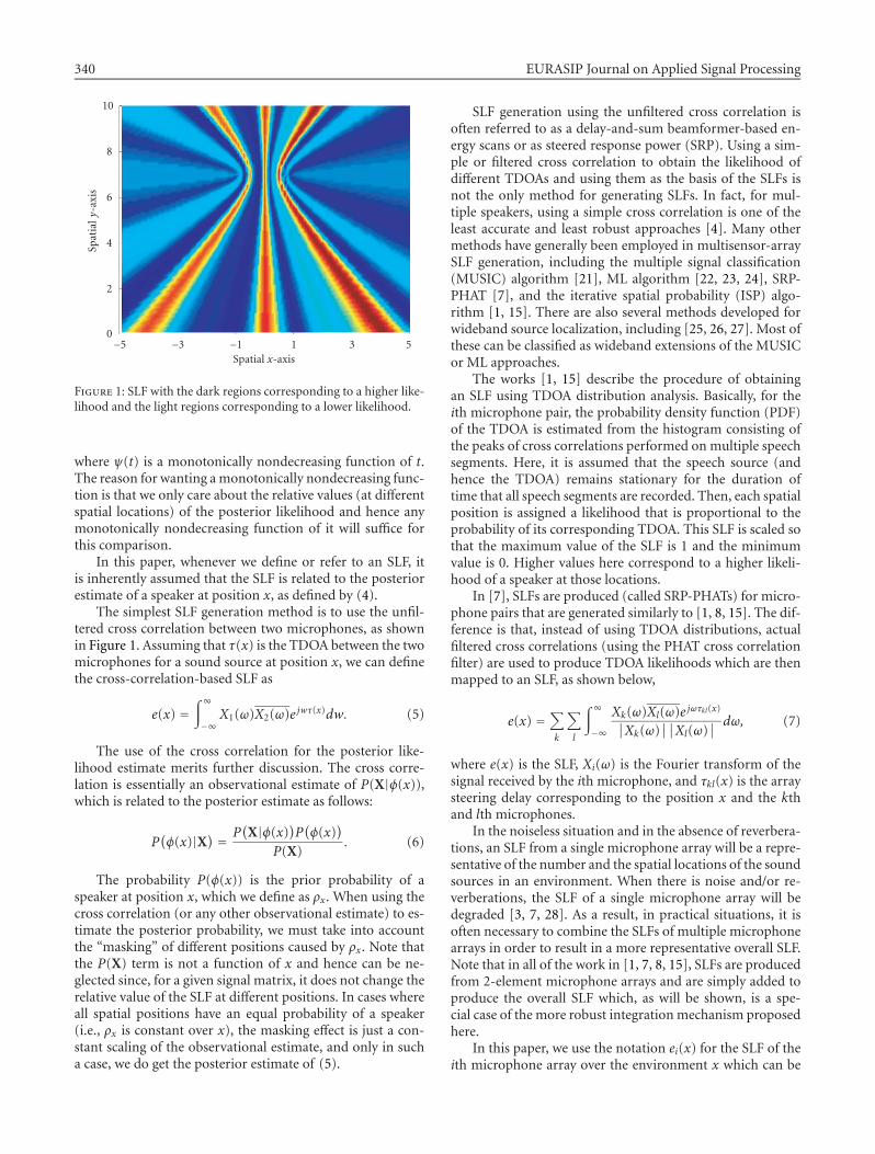
Figure 1: SLF with the dark regions corresponding to a higher like-lihood and the light regions corresponding to a lower likelihood.

where ψ(t) is a monotonically nondecreasing function of t.The reason for wanting amonotonically nondecreasing func-tion is that we only care about the relative values (at differentspatial locations) of the posterior likelihood and hence anymonotonically nondecreasing function of it will suffice forthis comparison.

In this paper, whenever we define or refer to an SLF, itis inherently assumed that the SLF is related to the posteriorestimate of a speaker at position x, as defined by (4).

The simplest SLF generation method is to use the unfil-tered cross correlation between two microphones, as shownin Figure 1. Assuming that τ(x) is the TDOA between the twomicrophones for a sound source at position x, we can definethe cross-correlation-based SLF as

e(x) =∫∞−∞

X1(ω)X2(ω)e jwτ(x)dw. (5)

The use of the cross correlation for the posterior like-lihood estimate merits further discussion. The cross corre-lation is essentially an observational estimate of P(X|φ(x)),which is related to the posterior estimate as follows:

P(φ(x)|X) = P

(X|φ(x))P(φ(x))

P(X). (6)

The probability P(φ(x)) is the prior probability of aspeaker at position x, which we define as ρx. When using thecross correlation (or any other observational estimate) to es-timate the posterior probability, we must take into accountthe “masking” of different positions caused by ρx. Note thatthe P(X) term is not a function of x and hence can be ne-glected since, for a given signal matrix, it does not change therelative value of the SLF at different positions. In cases whereall spatial positions have an equal probability of a speaker(i.e., ρx is constant over x), the masking effect is just a con-stant scaling of the observational estimate, and only in sucha case, we do get the posterior estimate of (5).

SLF generation using the unfiltered cross correlation isoften referred to as a delay-and-sum beamformer-based en-ergy scans or as steered response power (SRP). Using a sim-ple or filtered cross correlation to obtain the likelihood ofdifferent TDOAs and using them as the basis of the SLFs isnot the only method for generating SLFs. In fact, for mul-tiple speakers, using a simple cross correlation is one of theleast accurate and least robust approaches [4]. Many othermethods have generally been employed in multisensor-arraySLF generation, including the multiple signal classification(MUSIC) algorithm [21], ML algorithm [22, 23, 24], SRP-PHAT [7], and the iterative spatial probability (ISP) algo-rithm [1, 15]. There are also several methods developed forwideband source localization, including [25, 26, 27]. Most ofthese can be classified as wideband extensions of the MUSICor ML approaches.

The works [1, 15] describe the procedure of obtainingan SLF using TDOA distribution analysis. Basically, for theith microphone pair, the probability density function (PDF)of the TDOA is estimated from the histogram consisting ofthe peaks of cross correlations performed on multiple speechsegments. Here, it is assumed that the speech source (andhence the TDOA) remains stationary for the duration oftime that all speech segments are recorded. Then, each spatialposition is assigned a likelihood that is proportional to theprobability of its corresponding TDOA. This SLF is scaled sothat the maximum value of the SLF is 1 and the minimumvalue is 0. Higher values here correspond to a higher likeli-hood of a speaker at those locations.

In [7], SLFs are produced (called SRP-PHATs) for micro-phone pairs that are generated similarly to [1, 8, 15]. The dif-ference is that, instead of using TDOA distributions, actualfiltered cross correlations (using the PHAT cross correlationfilter) are used to produce TDOA likelihoods which are thenmapped to an SLF, as shown below,

e(x) =∑k

∑l

∫∞−∞

Xk(ω)Xl(ω)e jωτkl(x)∣∣Xk(ω)∣∣∣∣Xl(ω)

∣∣ dω, (7)

where e(x) is the SLF, Xi(ω) is the Fourier transform of thesignal received by the ith microphone, and τkl(x) is the arraysteering delay corresponding to the position x and the kthand lth microphones.

In the noiseless situation and in the absence of reverbera-tions, an SLF from a single microphone array will be a repre-sentative of the number and the spatial locations of the soundsources in an environment. When there is noise and/or re-verberations, the SLF of a single microphone array will bedegraded [3, 7, 28]. As a result, in practical situations, it isoften necessary to combine the SLFs of multiple microphonearrays in order to result in a more representative overall SLF.Note that in all of the work in [1, 7, 8, 15], SLFs are producedfrom 2-element microphone arrays and are simply added toproduce the overall SLF which, as will be shown, is a spe-cial case of the more robust integrationmechanism proposedhere.

In this paper, we use the notation ei(x) for the SLF of theith microphone array over the environment x which can be


0 0.2 0.4 0.6 0.8 1 1.2

x-distance to source in m (y-distance fixed at 3.5 m)

0

0.05

0.1

0.15

0.2

0.25

Observability

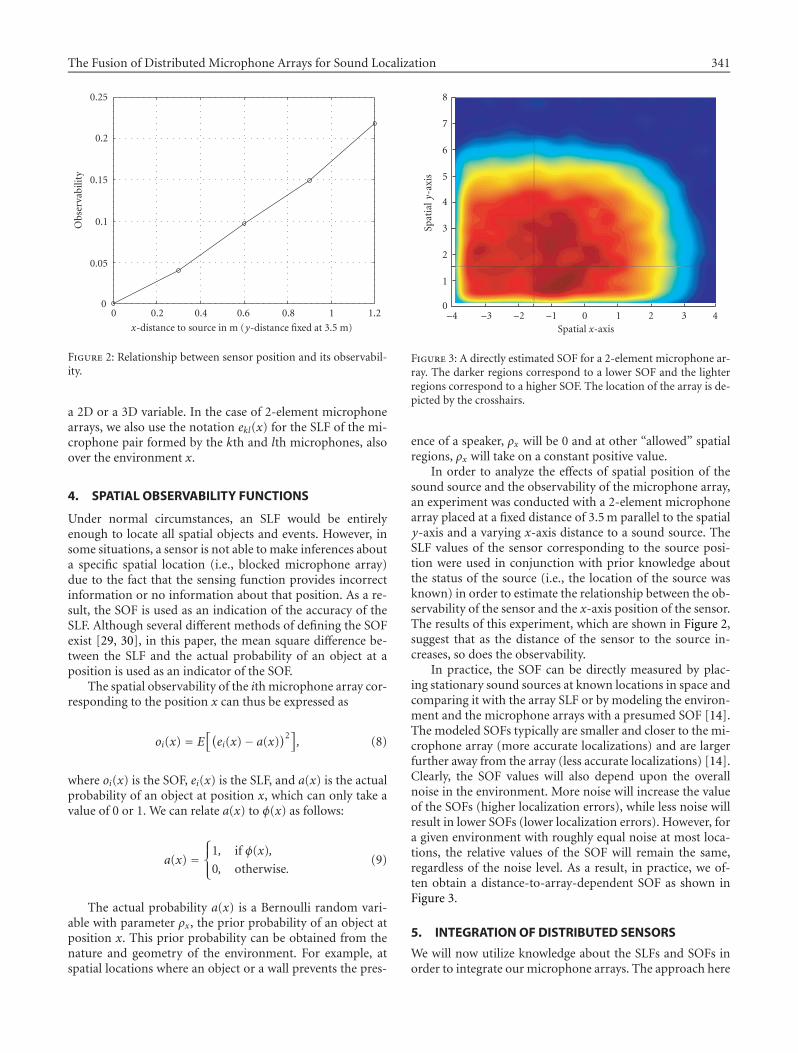
Figure 2: Relationship between sensor position and its observabil-ity.

a 2D or a 3D variable. In the case of 2-element microphonearrays, we also use the notation ekl(x) for the SLF of the mi-crophone pair formed by the kth and lth microphones, alsoover the environment x.

4. SPATIAL OBSERVABILITY FUNCTIONS

Under normal circumstances, an SLF would be entirelyenough to locate all spatial objects and events. However, insome situations, a sensor is not able to make inferences abouta specific spatial location (i.e., blocked microphone array)due to the fact that the sensing function provides incorrectinformation or no information about that position. As a re-sult, the SOF is used as an indication of the accuracy of theSLF. Although several different methods of defining the SOFexist [29, 30], in this paper, the mean square difference be-tween the SLF and the actual probability of an object at aposition is used as an indicator of the SOF.

The spatial observability of the ith microphone array cor-responding to the position x can thus be expressed as

oi(x) = E[(ei(x)− a(x)

)2], (8)

where oi(x) is the SOF, ei(x) is the SLF, and a(x) is the actualprobability of an object at position x, which can only take avalue of 0 or 1. We can relate a(x) to φ(x) as follows:

a(x) =1, if φ(x),

0, otherwise.(9)

The actual probability a(x) is a Bernoulli random vari-able with parameter ρx, the prior probability of an object atposition x. This prior probability can be obtained from thenature and geometry of the environment. For example, atspatial locations where an object or a wall prevents the pres-

−4 −3 −2 −1 0 1 2 3 4Spatial x-axis

0

1

2

3

4

5

6

7

8

Spatialy-axis

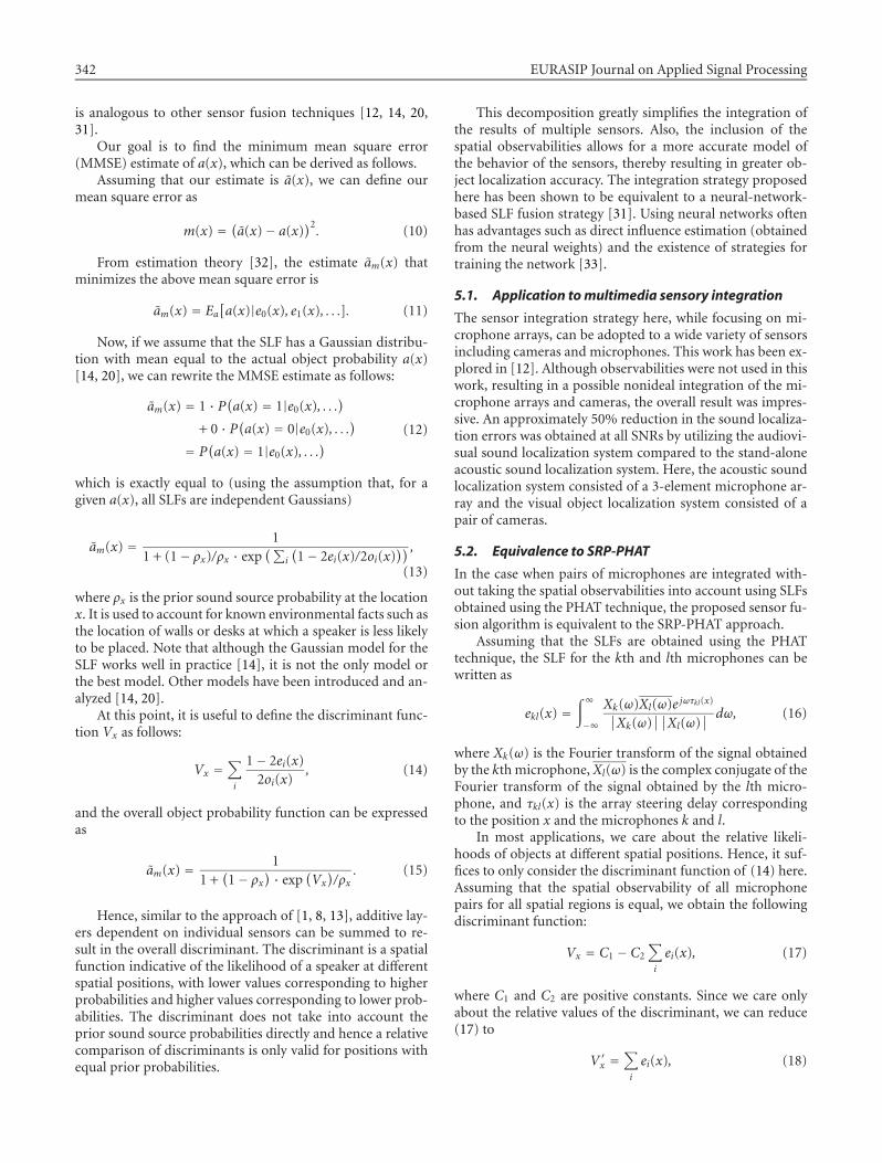
Figure 3: A directly estimated SOF for a 2-element microphone ar-ray. The darker regions correspond to a lower SOF and the lighterregions correspond to a higher SOF. The location of the array is de-picted by the crosshairs.

ence of a speaker, ρx will be 0 and at other “allowed” spatialregions, ρx will take on a constant positive value.

In order to analyze the effects of spatial position of thesound source and the observability of the microphone array,an experiment was conducted with a 2-element microphonearray placed at a fixed distance of 3.5m parallel to the spatialy-axis and a varying x-axis distance to a sound source. TheSLF values of the sensor corresponding to the source posi-tion were used in conjunction with prior knowledge aboutthe status of the source (i.e., the location of the source wasknown) in order to estimate the relationship between the ob-servability of the sensor and the x-axis position of the sensor.The results of this experiment, which are shown in Figure 2,suggest that as the distance of the sensor to the source in-creases, so does the observability.

In practice, the SOF can be directly measured by plac-ing stationary sound sources at known locations in space andcomparing it with the array SLF or by modeling the environ-ment and the microphone arrays with a presumed SOF [14].The modeled SOFs typically are smaller and closer to the mi-crophone array (more accurate localizations) and are largerfurther away from the array (less accurate localizations) [14].Clearly, the SOF values will also depend upon the overallnoise in the environment. More noise will increase the valueof the SOFs (higher localization errors), while less noise willresult in lower SOFs (lower localization errors). However, fora given environment with roughly equal noise at most loca-tions, the relative values of the SOF will remain the same,regardless of the noise level. As a result, in practice, we of-ten obtain a distance-to-array-dependent SOF as shown inFigure 3.

5. INTEGRATION OF DISTRIBUTED SENSORS

We will now utilize knowledge about the SLFs and SOFs inorder to integrate our microphone arrays. The approach here


is analogous to other sensor fusion techniques [12, 14, 20,31].

Our goal is to find the minimum mean square error(MMSE) estimate of a(x), which can be derived as follows.

Assuming that our estimate is a(x), we can define ourmean square error as

m(x) = (a(x)− a(x))2. (10)

From estimation theory [32], the estimate am(x) thatminimizes the above mean square error is

am(x) = Ea[a(x)|e0(x), e1(x), . . .]. (11)

Now, if we assume that the SLF has a Gaussian distribu-tion with mean equal to the actual object probability a(x)[14, 20], we can rewrite the MMSE estimate as follows:

am(x) = 1 · P(a(x) = 1|e0(x), . . .)

+ 0 · P(a(x) = 0|e0(x), . . .)

= P(a(x) = 1|e0(x), . . .

) (12)

which is exactly equal to (using the assumption that, for agiven a(x), all SLFs are independent Gaussians)

am(x) = 11 + (1− ρx)/ρx · exp

(∑i

(1− 2ei(x)/2oi(x)

)) ,(13)

where ρx is the prior sound source probability at the locationx. It is used to account for known environmental facts such asthe location of walls or desks at which a speaker is less likelyto be placed. Note that although the Gaussian model for theSLF works well in practice [14], it is not the only model orthe best model. Other models have been introduced and an-alyzed [14, 20].

At this point, it is useful to define the discriminant func-tion Vx as follows:

Vx =∑i

1− 2ei(x)2oi(x)

, (14)

and the overall object probability function can be expressedas

am(x) = 11 +

(1− ρx

) · exp (Vx)/ρx

. (15)

Hence, similar to the approach of [1, 8, 13], additive lay-ers dependent on individual sensors can be summed to re-sult in the overall discriminant. The discriminant is a spatialfunction indicative of the likelihood of a speaker at differentspatial positions, with lower values corresponding to higherprobabilities and higher values corresponding to lower prob-abilities. The discriminant does not take into account theprior sound source probabilities directly and hence a relativecomparison of discriminants is only valid for positions withequal prior probabilities.

This decomposition greatly simplifies the integration ofthe results of multiple sensors. Also, the inclusion of thespatial observabilities allows for a more accurate model ofthe behavior of the sensors, thereby resulting in greater ob-ject localization accuracy. The integration strategy proposedhere has been shown to be equivalent to a neural-network-based SLF fusion strategy [31]. Using neural networks oftenhas advantages such as direct influence estimation (obtainedfrom the neural weights) and the existence of strategies fortraining the network [33].

5.1. Application tomultimedia sensory integration

The sensor integration strategy here, while focusing on mi-crophone arrays, can be adopted to a wide variety of sensorsincluding cameras and microphones. This work has been ex-plored in [12]. Although observabilities were not used in thiswork, resulting in a possible nonideal integration of the mi-crophone arrays and cameras, the overall result was impres-sive. An approximately 50% reduction in the sound localiza-tion errors was obtained at all SNRs by utilizing the audiovi-sual sound localization system compared to the stand-aloneacoustic sound localization system. Here, the acoustic soundlocalization system consisted of a 3-element microphone ar-ray and the visual object localization system consisted of apair of cameras.

5.2. Equivalence to SRP-PHAT

In the case when pairs of microphones are integrated with-out taking the spatial observabilities into account using SLFsobtained using the PHAT technique, the proposed sensor fu-sion algorithm is equivalent to the SRP-PHAT approach.

Assuming that the SLFs are obtained using the PHATtechnique, the SLF for the kth and lth microphones can bewritten as

ekl(x) =∫∞−∞


∣∣ dω, (16)

where Xk(ω) is the Fourier transform of the signal obtainedby the kth microphone,Xl(ω) is the complex conjugate of theFourier transform of the signal obtained by the lth micro-phone, and τkl(x) is the array steering delay correspondingto the position x and the microphones k and l.

In most applications, we care about the relative likeli-hoods of objects at different spatial positions. Hence, it suf-fices to only consider the discriminant function of (14) here.Assuming that the spatial observability of all microphonepairs for all spatial regions is equal, we obtain the followingdiscriminant function:

Vx = C1 − C2

∑i

ei(x), (17)

where C1 and C2 are positive constants. Since we care onlyabout the relative values of the discriminant, we can reduce(17) to

V ′x =

∑i

ei(x), (18)


Distributed network of microphone arrays

Single equivalent microphone array

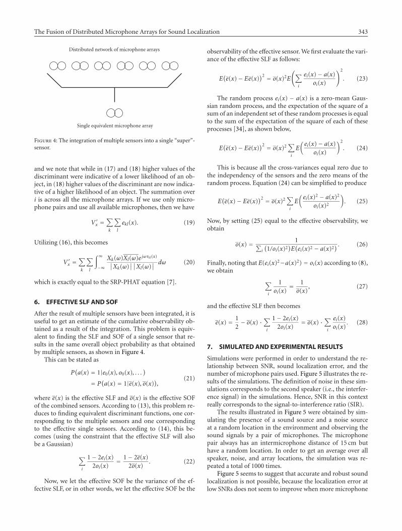
Figure 4: The integration of multiple sensors into a single “super”-sensor.

and we note that while in (17) and (18) higher values of thediscriminant were indicative of a lower likelihood of an ob-ject, in (18) higher values of the discriminant are now indica-tive of a higher likelihood of an object. The summation overi is across all the microphone arrays. If we use only micro-phone pairs and use all available microphones, then we have

V ′x =

∑k

∑l

ekl(x). (19)

Utilizing (16), this becomes

V ′x =

∑k

∑l

∫∞−∞


∣∣ dω (20)

which is exactly equal to the SRP-PHAT equation [7].

6. EFFECTIVE SLF AND SOF

After the result of multiple sensors have been integrated, it isuseful to get an estimate of the cumulative observability ob-tained as a result of the integration. This problem is equiv-alent to finding the SLF and SOF of a single sensor that re-sults in the same overall object probability as that obtainedby multiple sensors, as shown in Figure 4.

This can be stated as

P(a(x) = 1|e0(x), o0(x), . . .

)= P

(a(x) = 1|e(x), o(x)), (21)

where e(x) is the effective SLF and o(x) is the effective SOFof the combined sensors. According to (13), this problem re-duces to finding equivalent discriminant functions, one cor-responding to the multiple sensors and one correspondingto the effective single sensors. According to (14), this be-comes (using the constraint that the effective SLF will alsobe a Gaussian)

∑i

1− 2ei(x)2oi(x)

= 1− 2e(x)2o(x)

. (22)

Now, we let the effective SOF be the variance of the ef-fective SLF, or in other words, we let the effective SOF be the

observability of the effective sensor.We first evaluate the vari-ance of the effective SLF as follows:

E(e(x)− Ee(x)

)2 = o(x)2E

(∑i

ei(x)− a(x)oi(x)

)2

. (23)

The random process ei(x) − a(x) is a zero-mean Gaus-sian random process, and the expectation of the square of asum of an independent set of these random processes is equalto the sum of the expectation of the square of each of theseprocesses [34], as shown below,

E(e(x)− Ee(x)

)2 = o(x)2∑i

E(ei(x)− a(x)

oi(x)

)2. (24)

This is because all the cross-variances equal zero due tothe independency of the sensors and the zero means of therandom process. Equation (24) can be simplified to produce

E(e(x)− Ee(x)

)2 = o(x)2∑i

E(ei(x)2 − a(x)2

oi(x)2

). (25)

Now, by setting (25) equal to the effective observability, weobtain

o(x) = 1∑i

(1/oi(x)2

)E(ei(x)2 − a(x)2

) . (26)

Finally, noting that E(ei(x)2−a(x)2) = oi(x) according to (8),we obtain

∑i

1oi(x)

= 1o(x)

, (27)

and the effective SLF then becomes

e(x) = 12− o(x) ·

∑i

1− 2ei(x)2oi(x)

= o(x) ·∑i

ei(x)oi(x)

. (28)

7. SIMULATED AND EXPERIMENTAL RESULTS

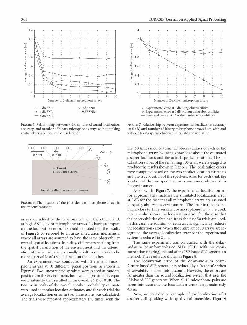
Simulations were performed in order to understand the re-lationship between SNR, sound localization error, and thenumber of microphone pairs used. Figure 5 illustrates the re-sults of the simulations. The definition of noise in these sim-ulations corresponds to the second speaker (i.e., the interfer-ence signal) in the simulations. Hence, SNR in this contextreally corresponds to the signal-to-interference ratio (SIR).

The results illustrated in Figure 5 were obtained by sim-ulating the presence of a sound source and a noise sourceat a random location in the environment and observing thesound signals by a pair of microphones. The microphonepair always has an intermicrophone distance of 15 cm buthave a random location. In order to get an average over allspeaker, noise, and array locations, the simulation was re-peated a total of 1000 times.

Figure 5 seems to suggest that accurate and robust soundlocalization is not possible, because the localization error atlow SNRs does not seem to improve when more microphone


1 2 3 4 5 6 7 8 9 10Number of 2-element microphone arrays

0

0.2

0.4

0.6

0.8

1

1.2

1.4

Average

localizationerror(m

)

1 dB SNR3 dB SNR5 dB SNR

7 dB SNR9 dB SNR

Figure 5: Relationship between SNR, simulated sound localizationaccuracy, and number of binary microphone arrays without takingspatial observabilities into consideration.

0.31 m 0.15 mWalls

2-elementmicrophone arrays

Sound localization test environment

Figure 6: The location of the 10 2-element microphone arrays inthe test environment.

arrays are added to the environment. On the other hand,at high SNRs, extra microphone arrays do have an impacton the localization error. It should be noted that the resultsof Figure 5 correspond to an array integration mechanismwhere all arrays are assumed to have the same observabilityover all spatial locations. In reality, differences resulting fromthe spatial orientation of the environment and the attenu-ation of the source signals usually result in one array to bemore observable of a spatial position than another.

An experiment was conducted with 2-element micro-phone arrays at 10 different spatial positions as shown inFigure 6. Two uncorrelated speakers were placed at randompositions in the environment, both with approximately equalvocal intensity that resulted in an overall SNR of 0 dB. Thetwo main peaks of the overall speaker probability estimatewere used as speaker location estimates, and for each trial theaverage localization error in two dimensions was calculated.The trials were repeated approximately 150 times, with the


0

0.2

0.4

0.6

0.8

1

1.2

1.4

Average

localizationerror(m

)

Experimental error at 0 dB using observabilitiesExperimental error at 0 dB without using observabilitiesSimulated error at 0 dB without using observabilities

Figure 7: Relationship between experimental localization accuracy(at 0 dB) and number of binary microphone arrays both with andwithout taking spatial observabilities into consideration.

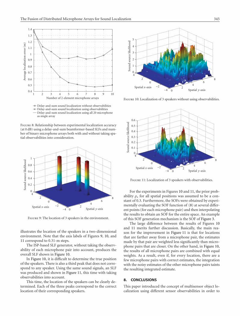
first 50 times used to train the observabilities of each of themicrophone arrays by using knowledge about the estimatedspeaker locations and the actual speaker locations. The lo-calization errors of the remaining 100 trials were averaged toproduce the results shown in Figure 7. The localization errorswere computed based on the two speaker location estimatesand the true location of the speakers. Also, for each trial, thelocation of the two speech sources was randomly varied inthe environment.

As shown in Figure 7, the experimental localization er-ror approximately matches the simulated localization errorat 0 dB for the case that all microphone arrays are assumedto equally observe the environment. The error in this case re-mains close to 1m even as more microphone arrays are used.Figure 7 also shows the localization error for the case thatthe observabilities obtained from the first 50 trials are used.In this case, the addition of extra arrays significantly reducesthe localization error. When the entire set of 10 arrays are in-tegrated, the average localization error for the experimentalsystem is reduced to 8 cm.

The same experiment was conducted with the delay-and-sum beamformer-based SLFs (SRPs with no cross-correlation filtering) instead of the ISP-based SLF generationmethod. The results are shown in Figure 8.

The localization error of the delay-and-sum beam-former-based SLF generator is reduced by a factor of 2 whenobservability is taken into account. However, the errors arefar greater than the sound localization system that uses theISP-based SLF generator. When all 10 microphone pairs aretaken into account, the localization error is approximately0.5m.

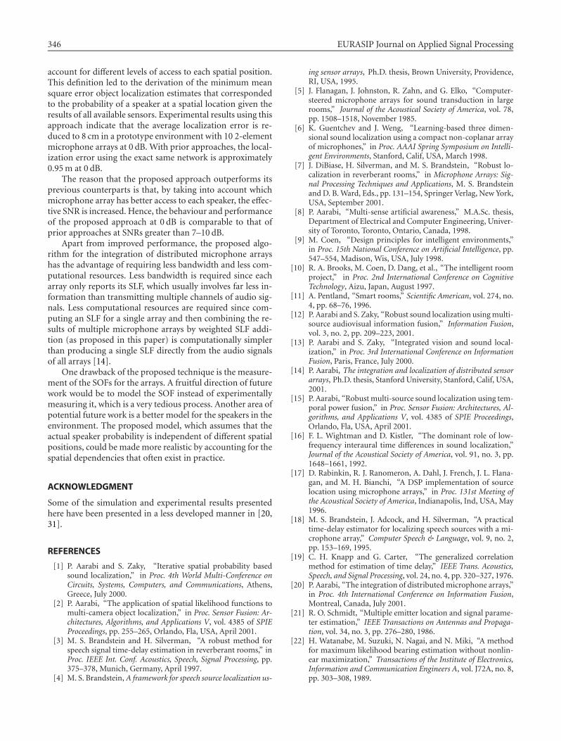
Now, we consider an example of the localization of 3speakers, all speaking with equal vocal intensities. Figure 9



0.4

0.5

0.6

0.7

0.8

0.9

1

1.1

1.2

1.3

1.4

Average

localizationerror(m

)

Delay-and-sum sound localization without observabilitiesDelay-and-sum sound localization using observabilitiesDelay-and-sum sound localization using all 20 microphoneas single array

Figure 8: Relationship between experimental localization accuracy(at 0 dB) using a delay-and-sum beamformer-based SLFs and num-ber of binary microphone arrays both with and without taking spa-tial observabilities into consideration.

02

46

8

Spatial y-axis

42

0−2

−4Spatial x-axis

0

0.2

0.4

0.6

0.8

1

Soundsourcelikelihoo

d

Figure 9: The location of 3 speakers in the environment.

illustrates the location of the speakers in a two-dimensionalenvironment. Note that the axis labels of Figures 9, 10, and11 correspond to 0.31-m steps.

The ISP-based SLF generator, without taking the observ-ability of each microphone pair into account, produces theoverall SLF shown in Figure 10.

In Figure 10, it is difficult to determine the true positionof the speakers. There is also a third peak that does not corre-spond to any speaker. Using the same sound signals, an SLFwas produced and shown in Figure 11, this time with takingobservabilities into account.

This time, the location of the speakers can be clearly de-termined. Each of the three peaks correspond to the correctlocation of their corresponding speakers.

02

46

8

Spatial y-axis

42

0−2

−4Spatial x-axis

0

1

2

3

4

5


d

Figure 10: Localization of 3 speakers without using observabilities.

02

46

8

Spatial y-axis

42

0−2

−4Spatial x-axis

0

0.1

0.2

0.3

0.4

0.5

0.6


d

Figure 11: Localization of 3 speakers with observabilities.

For the experiments in Figures 10 and 11, the prior prob-ability ρx for all spatial positions was assumed to be a con-stant of 0.3. Furthermore, the SOFs were obtained by experi-mentally evaluating the SOF function of (8) at several differ-ent points (for eachmicrophone pair) and then interpolatingthe results to obtain an SOF for the entire space. An exampleof this SOF generation mechanism is the SOF of Figure 3.

The large difference between the results of Figures 10and 11 merits further discussion. Basically, the main rea-son for the improvement in Figure 11 is that for locationsthat are farther away from a microphone pair, the estimatesmade by that pair are weighted less significantly than micro-phone pairs that are closer. On the other hand, in Figure 10,the results of all microphone pairs are combined with equalweights. As a result, even if, for every location, there are afew microphone pairs with correct estimates, the integrationwith the noisy estimates of the other microphone pairs taintsthe resulting integrated estimate.

8. CONCLUSIONS

This paper introduced the concept of multisensor object lo-calization using different sensor observabilities in order to


account for different levels of access to each spatial position.This definition led to the derivation of the minimum meansquare error object localization estimates that correspondedto the probability of a speaker at a spatial location given theresults of all available sensors. Experimental results using thisapproach indicate that the average localization error is re-duced to 8 cm in a prototype environment with 10 2-elementmicrophone arrays at 0 dB. With prior approaches, the local-ization error using the exact same network is approximately0.95m at 0 dB.

The reason that the proposed approach outperforms itsprevious counterparts is that, by taking into account whichmicrophone array has better access to each speaker, the effec-tive SNR is increased. Hence, the behaviour and performanceof the proposed approach at 0 dB is comparable to that ofprior approaches at SNRs greater than 7–10 dB.

Apart from improved performance, the proposed algo-rithm for the integration of distributed microphone arrayshas the advantage of requiring less bandwidth and less com-putational resources. Less bandwidth is required since eacharray only reports its SLF, which usually involves far less in-formation than transmitting multiple channels of audio sig-nals. Less computational resources are required since com-puting an SLF for a single array and then combining the re-sults of multiple microphone arrays by weighted SLF addi-tion (as proposed in this paper) is computationally simplerthan producing a single SLF directly from the audio signalsof all arrays [14].

One drawback of the proposed technique is the measure-ment of the SOFs for the arrays. A fruitful direction of futurework would be to model the SOF instead of experimentallymeasuring it, which is a very tedious process. Another area ofpotential future work is a better model for the speakers in theenvironment. The proposed model, which assumes that theactual speaker probability is independent of different spatialpositions, could be made more realistic by accounting for thespatial dependencies that often exist in practice.

ACKNOWLEDGMENT

Some of the simulation and experimental results presentedhere have been presented in a less developed manner in [20,31].

REFERENCES

[1] P. Aarabi and S. Zaky, “Iterative spatial probability basedsound localization,” in Proc. 4th World Multi-Conference onCircuits, Systems, Computers, and Communications, Athens,Greece, July 2000.

[2] P. Aarabi, “The application of spatial likelihood functions tomulti-camera object localization,” in Proc. Sensor Fusion: Ar-chitectures, Algorithms, and Applications V, vol. 4385 of SPIEProceedings, pp. 255–265, Orlando, Fla, USA, April 2001.

[3] M. S. Brandstein and H. Silverman, “A robust method forspeech signal time-delay estimation in reverberant rooms,” inProc. IEEE Int. Conf. Acoustics, Speech, Signal Processing, pp.375–378, Munich, Germany, April 1997.

[4] M. S. Brandstein, A framework for speech source localization us-

ing sensor arrays, Ph.D. thesis, Brown University, Providence,RI, USA, 1995.

[5] J. Flanagan, J. Johnston, R. Zahn, and G. Elko, “Computer-steered microphone arrays for sound transduction in largerooms,” Journal of the Acoustical Society of America, vol. 78,pp. 1508–1518, November 1985.

[6] K. Guentchev and J. Weng, “Learning-based three dimen-sional sound localization using a compact non-coplanar arrayof microphones,” in Proc. AAAI Spring Symposium on Intelli-gent Environments, Stanford, Calif, USA, March 1998.

[7] J. DiBiase, H. Silverman, and M. S. Brandstein, “Robust lo-calization in reverberant rooms,” in Microphone Arrays: Sig-nal Processing Techniques and Applications, M. S. Brandsteinand D. B.Ward, Eds., pp. 131–154, Springer Verlag, New York,USA, September 2001.

[8] P. Aarabi, “Multi-sense artificial awareness,” M.A.Sc. thesis,Department of Electrical and Computer Engineering, Univer-sity of Toronto, Toronto, Ontario, Canada, 1998.

[9] M. Coen, “Design principles for intelligent environments,”in Proc. 15th National Conference on Artificial Intelligence, pp.547–554, Madison, Wis, USA, July 1998.

[10] R. A. Brooks, M. Coen, D. Dang, et al., “The intelligent roomproject,” in Proc. 2nd International Conference on CognitiveTechnology, Aizu, Japan, August 1997.

[11] A. Pentland, “Smart rooms,” Scientific American, vol. 274, no.4, pp. 68–76, 1996.

[12] P. Aarabi and S. Zaky, “Robust sound localization usingmulti-source audiovisual information fusion,” Information Fusion,vol. 3, no. 2, pp. 209–223, 2001.

[13] P. Aarabi and S. Zaky, “Integrated vision and sound local-ization,” in Proc. 3rd International Conference on InformationFusion, Paris, France, July 2000.

[14] P. Aarabi, The integration and localization of distributed sensorarrays, Ph.D. thesis, Stanford University, Stanford, Calif, USA,2001.

[15] P. Aarabi, “Robustmulti-source sound localization using tem-poral power fusion,” in Proc. Sensor Fusion: Architectures, Al-gorithms, and Applications V, vol. 4385 of SPIE Proceedings,Orlando, Fla, USA, April 2001.

[16] F. L. Wightman and D. Kistler, “The dominant role of low-frequency interaural time differences in sound localization,”Journal of the Acoustical Society of America, vol. 91, no. 3, pp.1648–1661, 1992.

[17] D. Rabinkin, R. J. Ranomeron, A. Dahl, J. French, J. L. Flana-gan, and M. H. Bianchi, “A DSP implementation of sourcelocation using microphone arrays,” in Proc. 131st Meeting ofthe Acoustical Society of America, Indianapolis, Ind, USA, May1996.

[18] M. S. Brandstein, J. Adcock, and H. Silverman, “A practicaltime-delay estimator for localizing speech sources with a mi-crophone array,” Computer Speech & Language, vol. 9, no. 2,pp. 153–169, 1995.

[19] C. H. Knapp and G. Carter, “The generalized correlationmethod for estimation of time delay,” IEEE Trans. Acoustics,Speech, and Signal Processing, vol. 24, no. 4, pp. 320–327, 1976.

[20] P. Aarabi, “The integration of distributedmicrophone arrays,”in Proc. 4th International Conference on Information Fusion,Montreal, Canada, July 2001.

[21] R. O. Schmidt, “Multiple emitter location and signal parame-ter estimation,” IEEE Transactions on Antennas and Propaga-tion, vol. 34, no. 3, pp. 276–280, 1986.

[22] H. Watanabe, M. Suzuki, N. Nagai, and N. Miki, “A methodfor maximum likelihood bearing estimation without nonlin-ear maximization,” Transactions of the Institute of Electronics,Information and Communication Engineers A, vol. J72A, no. 8,pp. 303–308, 1989.


[23] H. Watanabe, M. Suzuki, N. Nagai, and N. Miki, “Maximumlikelihood bearing estimation by quasi-Newton method us-ing a uniform linear array,” in Proc. IEEE Int. Conf. Acoustics,Speech, Signal Processing, pp. 3325–3328, Toronto, Ontario,Canada, April 1991.

[24] I. Ziskind and M. Wax, “Maximum likelihood localiza-tion of multiple sources by alternating projection,” IEEETrans. Acoustics, Speech, and Signal Processing, vol. 36, no. 10,pp. 1553–1560, 1988.

[25] H. Wang and M. Kaveh, “Coherent signal-subspace process-ing for the detection and estimation of angles of arrival ofmultiple wide-band sources,” IEEE Trans. Acoustics, Speech,and Signal Processing, vol. 33, no. 4, pp. 823–831, 1985.

[26] S. Valaee and P. Kabal, “Wide-band array processing usinga two-sided correlation transformation,” IEEE Trans. SignalProcessing, vol. 43, no. 1, pp. 160–172, 1995.

[27] B. Friedlander and A. J. Weiss, “Direction finding for wide-band signals using an interpolated array,” IEEE Trans. SignalProcessing, vol. 41, no. 4, pp. 1618–1634, 1993.

[28] P. Aarabi and A. Mahdavi, “The relation between speechsegment selectivity and time-delay estimation accuracy,” inProc. IEEE Int. Conf. Acoustics, Speech, Signal Processing, Or-lando, Fla, USA, May 2002.

[29] S. S. Iyengar and D. Thomas, “A distributed sensor networkstructure with fault tolerant facilities,” in Intelligent Controland Adaptive Systems, vol. 1196 of SPIE Proceedings, Philadel-phia, Pa, USA, November 1989.

[30] R. R. Brooks and S. S. Iyengar, Multi-Sensor Fusion: Funda-mentals and Applications with Software, Prentice Hall, UpperSaddle River, NJ, USA, 1998.

[31] P. Aarabi, “The equivalence of Bayesian multi-sensor infor-mation fusion and neural networks,” in Proc. Sensor Fusion:Architectures, Algorithms, and Applications V, vol. 4385 of SPIEProceedings, Orlando, Fla, USA, April 2001.

[32] A. Leon-Garcia, Probability and Random Processes for Electri-cal Engineering, Addison-Wesley, Reading, Mass, USA, 2ndedition, 1994.

[33] B. Widrow and S. D. Stearns, Adaptive Signal Processing,Prentice-Hall, Englewood Cliffs, NJ, USA, 1985.

[34] A. Papoulis, Probability, Random Variables and Stochastic Pro-cesses, McGraw-Hill, New York, NY, USA, 2nd edition, 1984.

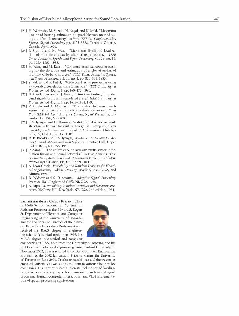
Parham Aarabi is a Canada Research Chairin Multi-Sensor Information Systems, anAssistant Professor in the Edward S. RogersSr. Department of Electrical and ComputerEngineering at the University of Toronto,and the Founder and Director of the Artifi-cial Perception Laboratory. Professor Aarabireceived his B.A.S. degree in engineer-ing science (electrical option) in 1998, hisM.A.S. degree in electrical and computerengineering in 1999, both from the University of Toronto, and hisPh.D. degree in electrical engineering from Stanford University. InNovember 2002, he was selected as the Best Computer EngineeringProfessor of the 2002 fall session. Prior to joining the Universityof Toronto in June 2001, Professor Aarabi was a Coinstructor atStanford University as well as a Consultant to various silicon valleycompanies. His current research interests include sound localiza-tion, microphone arrays, speech enhancement, audiovisual signalprocessing, human-computer interactions, and VLSI implementa-tion of speech processing applications.

Documents

TheFusionofDistributedMicrophoneArrays forSoundLocalizationThe Fusion of Distributed Microphone Arrays for Sound Localization 339 2. BASICSOUNDLOCALIZATION Sound localization is accomplished