The Young, the Old, and the Restless: Demographics and Business

804

American Economic Review 2009, 99:3, 804–826http://www.aeaweb.org/articles.php?doi=10.1257/aer.99.3.804

The baby boom and subsequent baby bust in the United States resulted in dramatic shifts in the age composition of the American population. Japan, Germany, and other industrialized countries have experienced similarly dramatic demographic change during the postwar period, although the details regarding timing and nature differ from place to place. In this paper, we investigate the consequences of demographic change for business cycle analysis.

Recently, a great deal of attention has been devoted to studying the moderation in business cycle volatility in the US since the mid-1980s. Less attention has been paid, however, to the run-up in volatility that began in the mid-1960s. We propose demographic change as a framework that can rationalize the evolution of US macroeconomic volatility over the last four decades. Moreover, we offer this framework as relevant for understanding the evolution of cyclical volatil-ity observed in other industrialized economies during the postwar period. Specifically, we find that changes in the age composition of the workforce account for a significant fraction of the variation in business cycle volatility observed in the US and the rest of the G7.

We establish the relationship between demographics and macroeconomic volatility in the fol-lowing manner. First, we document important differences in the responsiveness of labor market activity to the business cycle for individuals of different ages. In previous work, Kim B. Clark and Lawrence H. Summers (1981), José-Víctor Ríos-Rull (1996), and Paul Gomme et al. (2005) showed, using postwar US data, that the cyclical volatility of market work is U-shaped as a func-tion of age. The young experience much greater volatility of employment and hours worked than the prime-aged over the business cycle; those closer to retirement experience volatility some-where in between. Our first contribution is to show that this is an empirical regularity for all G7 countries.

The Young, the Old, and the Restless: Demographics and Business Cycle Volatility

By Nir Jaimovich and Henry E. Siu*

We investigate the consequences of demographic change for business cycle analysis. We find that changes in the age composition of the labor force account for a significant fraction of the variation in cyclical volatility observed in the G7. Since World War II, these countries have experienced dramatic demo-graphic changes, although details regarding timing and nature differ across countries. We exploit this variation to show that the workforce age composition has a large and significant effect on cyclical volatility. We relate our results to the recent decline in US macroeconomic volatility, finding that demographic change accounts for approximately one-fifth to one-third of this moderation. (JEL E32, J11)

* Jaimovich: Department of Economics, Stanford University, 579 Serra Mall, Stanford, CA, 94305, and National Bureau of Economic Research (e-mail: [email protected]); Siu: Department of Economics, University of British Columbia, 997–1873 East Mall, Vancouver, BC, V6T 1Z1 (e-mail: [email protected]). We thank the anony-mous referees, Manuel Amador, Gadi Barlevy, Paul Beaudry, Larry Christiano, Julie Cullen, Marty Eichenbaum, David Green, Karen Kopecky, Valerie Ramey, Sergio Rebelo, Víctor Ríos-Rull, Jim Sullivan, and numerous workshop and seminar participants for helpful comments. Hide Mizobuchi, Subrata Sarker, Shun Wang, and especially Seth Pruitt and Josie Smith, provided expert research assistance. Part of this work was completed while Siu was a visiting scholar at the Federal Reserve Bank of Minneapolis during the 2006–2007 academic year, and he thanks them for their support and hospitality. Siu also thanks the Social Sciences and Humanities Research Council of Canada for support.

VOL. 99 NO. 3 805JAImOVIch ANd SIU: dEmOGRAphIcS ANd BUSINESS cycLE VOLAtILIty

Specifically, we show in Section I that the volatility of market work is U-shaped as a function of age. For example, when averaged across countries, the standard deviation of cyclical employ-ment fluctuations for 15- 19-year-olds is nearly six times greater than that of 40- 49-year-olds; as a result, although teenagers comprise only 6 percent of aggregate employment, they account for 17 percent of aggregate employment volatility. Similarly, the average employment volatility of 60- 64-year-olds is about three times greater than that of 40- 49-year-olds.

Given this observation, a natural conjecture is that the responsiveness of aggregate output to business cycle shocks depends on the age composition of the workforce. For instance, suppose that the volatility of age-specific employment is unaffected by age composition. Then, when an economy is characterized by a large share of young workers, all else equal, these should be periods of greater cyclical volatility in market work and output than would otherwise occur. Our second contribution is to show that this is indeed the case.

During the postwar period, the G7 countries experienced substantial variation in business cycle volatility. Variation in the nature of demographic change across countries allows us to identify the effect of workforce age composition. In Section II, we use panel-data methods to show that the age composition has a quantitatively large and statistically significant effect on measures of business cycle volatility. Because workforce composition is largely determined by fertility decisions made at least 15 years prior to current volatility, we are able to obtain unbiased inference on the causal effect using standard econometric techniques.

In Section III, we relate these findings to the recent literature on “The Great Moderation”—the decline in macroeconomic volatility experienced in the US since the mid-1980s.1 Through simple quantitative accounting exercises, we find that demographic change accounts for roughly one-fifth to one-third of the moderation experienced in the US. Clearly, demographic change is not the sole factor responsible for this episode; nevertheless, demographic change serves as a common factor relevant for understanding the evolution of business cycle volatility—not only in the US, but also in other G7 countries—over the past four decades.2 We provide concluding remarks in Section IV.

I. Differences in Market Work Volatility by Age

In this section, we analyze the responsiveness of market work to the business cycle for data disaggregated by age. We begin with an analysis of the US and Japan, countries for which con-sistent information on hours worked by age is available. We then document differences in the cyclical volatility of employment by age in the sample of industrialized economies represented by the G7.

A. Evidence on hours Worked from the US and Japan

Our approach to studying differences in business cycle volatility by age is similar to that of Gomme et al. (2005). We use data from the March supplement of the Current Population Survey (CPS) to construct annual series of per capita hours worked from 1963 to 2005 for specific age groups, as well as an aggregate series for all individuals 15 years of age and older. For Japan, we construct age-specific, annual time series covering 1972 to 2004, using data from the Annual

1 See Chang-Jin Kim and Charles R. Nelson (1999) and Margaret M. McConnell and Gabriel Perez-Quiros (2000) for early papers identifying a change in output growth volatility. The term “The Great Moderation” is first used to describe this phenomenon by James H. Stock and Mark W. Watson (2003), and more recently by Ben S. Bernanke (2004).

2 See also Olivier Blanchard and John Simon (2001) and Stock and Watson (2005) for analysis of the G7.

JUNE 2009806 thE AmERIcAN EcONOmIc REVIEW

Report of the Labour Force Survey. See Appendix A for detailed information on data sources used throughout the paper.

The age-specific hours-worked series display low frequency variation due, for instance, to changes in female labor force participation and trends in schooling and retirement. As such, we remove the trend from each series using the Hodrick-Prescott (HP) filter. We follow the recent work of Morten O. Ravn and Harald Uhlig (2002), who show that the appropriate value of the smoothing parameter is 6.25 for annual data, when isolating fluctuations at the traditional busi-ness cycle frequencies (those higher than eight years).3

Table 1 presents results for the volatility of hours worked in the US for various age groups. The first row presents the percent standard deviation of the filtered age-specific series. We see a distinct U-shaped pattern in the volatility of hours by age.

We are not interested in the high frequency fluctuations in these time series per se, but rather those that are correlated with the business cycle. For each age-specific series, we identify the business cycle component as the projection on a constant, current detrended output, and on cur-rent and lagged detrended aggregate hours; we refer to these as the cyclical hours worked series. The second row of Table 1 reports the R2 from these regressions. This is very high for most age groups, indicating that the preponderance of high frequency fluctuations is attributable to the business cycle. The exceptions are the 60–64 and the 65+ age groups. Here, a larger fraction of fluctuations are due to age-specific, noncyclical shocks.

The third row indicates the percent standard deviation of the cyclical age-specific series. Compared to row one, the largest differences between filtered and cyclical volatilities are for those age 60 years and older, reflecting the discussion of the previous paragraph. Nevertheless, the U-shaped pattern remains. The young experience much greater cyclical volatility in hours than those in their prime; the volatility of those at retirement age is somewhere in between. Moreover, the differences across age groups are large. The standard deviation of cyclical hours fluctuations for 15- 19-year-old and 20- 24-year-old workers is at least 5.5 and 2.5 times that of 50- 59-year-olds, respectively. Relative to the 50- 59-year-olds, hours worked is almost twice as volatile for the 25–29 and 65+ age groups.4

The fourth row indicates the average share of aggregate hours worked during the sample period by each age group. The last row indicates the share of “aggregate hours volatility” attrib-utable to each age group. Here, aggregate hours volatility is represented by the hours-weighted average of age-specific cyclical volatilities. What is striking is the extent to which fluctuations in aggregate hours are disproportionately accounted for by young workers. Although those age 15–29 make up only 26 percent of aggregate hours worked, they account for 44 percent of aggre-gate hours volatility. By contrast, prime-age workers in their 40s and 50s account for 41 percent of hours but only 27 percent of hours volatility.

3 Using a similar approach, Craig Burnside (2000) arrives at a value of 6.66. Based on visual inspection of the HP filter’s transfer function, Marianne Baxter and Robert G. King (1999) recommend a value of ten. Throughout this paper, we have repeated our analysis of annual data using all of these smoothing parameter values with the HP filter, in addi-tion to the band-pass filter proposed by Baxter and King, in order to isolate fluctuations between two and eight years in frequency. The results are virtually identical in all cases. By contrast, much of the macroeconomics literature has used a smoothing parameter of 100 with the HP filter for annual data. Though not reported here, we have repeated our analysis with this choice, and the results are very similar. See an earlier draft of this paper, Jaimovich and Siu (2007), for details.

4 These results corroborate the findings of Gomme et al. (2005), and extend them to include data from the 2001 recession. See also Clark and Summers (1981), James W. Moser (1986), Ríos-Rull (1996), and Éva Nagypál (2005), who document differences in cyclical sensitivity across age groups. More broadly, the literature documents differences as a function of skill; see for instance, Finn E. Kydland and Edward C. Prescott (1993) and Hilary Hoynes (2000), and the references therein. Note that those studies are confined to the analysis of US data.


These large differences by age remain when we undertake further demographic breakdowns. These results are presented in Appendix B and summarized here. We first disaggregate the US workforce by age and educational attainment. For brevity, we present results only for two education groups: those with high school diplomas or less (labeled less education), and those with at least some postsecondary education (more education). Several observations deserve mention.

First, there is a noticeable difference in the volatility of hours by education. Interestingly, the differences across education are much less pronounced for young workers than for the prime-aged. A simple average across those age 20–24 and 25–29 indicates that persons with less edu-cation have hours volatility that is 1.5 times that of those with more; by contrast, the difference across education groups is a factor of 2.5 for those age 30–59. Note that large differences by age remain for both education groups. For instance, 20- 24-year-olds experience hours volatil-ity 2.5 to 3 times greater than 40- 49-year-olds, regardless of educational attainment. Indeed, 20- 29-year-olds with more education have greater volatility than prime-age workers with less education.

Appendix B also presents results disaggregated by age and gender. Again, the U-shaped pattern exists for both men and women. Moreover, the magnitude of volatility differences by age is roughly similar. Importantly, the differences across age groups within gender are much more pronounced than the differences across genders within age groups. An average across age groups indicates that males have 10 percent higher hours volatility over the cycle. On the other hand, those age 15–19 and 20–24 experience hours fluctuations that are roughly 5.5 and 3 times more volatile than those 50–59, for either gender. Gomme et al. (2004) discuss age differences with further demographic breakdowns (e.g., marital status, industry of occupation) for the US. Their results corroborate those presented here, indicating large and important differences in the volatility of hours worked by age.

Table 2 presents the same calculations as shown in Table 1 for Japan. As in the US, there is a U-shaped pattern to both the filtered and the cyclical volatility of hours as a function of age. Several differences between the two countries deserve mention.

First, the volatility of hours worked is smaller in Japan overall. Second, the regression R2s for those age 60+ are larger in Japan than in the US, indicating that hours fluctuations for these workers are more correlated with the business cycle. Third, the volatility of teenagers and those age 65+ relative to the prime-aged is very similar to that found in the US. For the remaining age groups, the differences are not as pronounced, although significant differences by age remain. Finally, individuals over the age of 60 in Japan are more significant contributors to the volatility of aggregate hours than those in the US. This is due to their larger hours share and their greater age-specific cyclical volatility. In fact, except for teenagers, the 65+ group experiences greater cyclical volatility in hours worked than any other age group.

Table 1—Volatility of Hours Worked by Age Groups, US

15–19 20–24 25–29 30–39 40–49 50–59 60–64 65+Filtered volatility 4.351 2.130 1.471 1.073 0.790 0.824 1.309 2.839R2 0.79 0.80 0.83 0.88 0.89 0.72 0.30 0.22Cyclical volatility 3.868 1.902 1.318 1.014 0.752 0.705 0.708 1.331Percentage of hours 3.24 10.33 12.86 25.38 23.29 17.20 4.82 2.88Percentage of hours volatility 11.22 17.58 15.17 23.03 15.67 10.86 3.05 3.43

Note: HP-filtered data from the March current population Survey, 1963–2005.


B. Evidence on Employment from the G7

We provide further evidence of the differences across age groups in business cycle volatility by considering data for the G7 economies. Because data on hours worked disaggregated by age are not available for all countries, we restrict our attention to employment. The data we analyze are from published and unpublished national government sources, and the Organisation for Economic Co-operation and Development (OECD) Labour Force Statistics database. The data are at an annual frequency, and the time coverage varies across countries. See Appendix A for details.

We identify cyclical fluctuations in the data as we did in our analysis of hours worked. For many of the G7 countries, the high frequency fluctuations of those age 65 and older are largely orthogo-nal to the business cycle. For instance, from the regression of the 65+ age group on aggregate employment and output, the R2 for France is only 0.04. In Italy, employment for this group is actu-ally negatively correlated with the cycle. As a result, for all countries except Japan, we omit those age 65 years and older, and define aggregate employment as that among 15- to 64-year-olds.5 We retain this older group for Japan since their age-specific employment regression produces an R2 of 0.67, indicating that employment among the old is highly correlated with the cycle.

Table 3 presents our results for HP-filtered data from the G7. For brevity, the information dis-played is condensed relative to Tables 1 and 2. Because postwar aggregate employment volatility varies widely across countries, we normalize the age-specific measures relative to the volatility of 40- 49-year-olds.

Again, the age profile of business cycle employment volatility can be characterized as roughly U-shaped, with large differences across age groups.6 The young and old display greater cyclical sensitivity than prime-aged individuals. In all countries, the 15- 29-year-olds are substantially more volatile than those age 30–59. This is particularly true for the continental European coun-tries. Taking a simple average across all G7 countries, we find that while the young comprise 30 percent of aggregate employment, they account for approximately 50 percent of aggregate employment volatility. Large differences between the prime-aged and those over 60 are also evident in Europe and Japan. In each of these countries, this older group also contributes dispro-portionately to aggregate volatility.

To summarize, we find that age-specific differences in business cycle responsiveness of market work are an empirical regularity in our sample of industrialized economies. Our findings extend the results of Clark and Summers (1981), Ríos-Rull (1996), and Gomme et al. (2004) for the US to the rest of the G7. That these economies differ greatly in terms of industry composition, and the degree of labor market regulation makes this finding all the more striking. These results suggest

5 Since the 65+ share of the labor force and employment is small, our results are unchanged if we include this group in our analysis.

6 See Gomme et al. (2004) for similar results for several OECD countries.

Table 2—Volatility of Hours Worked by Age Groups, Japan

15–19 20–24 25–29 30–39 40–49 50–59 60–64 65+Filtered volatility 2.651 0.936 0.780 0.695 0.580 0.606 0.943 1.084R2 0.64 0.64 0.84 0.87 0.88 0.91 0.42 0.54Cyclical volatility 2.142 0.745 0.727 0.658 0.551 0.586 0.605 0.792Percentage of hours 2.21 10.18 11.77 23.34 24.19 18.67 4.92 4.73Percentage of hours volatility 7.05 11.08 12.75 22.90 19.89 16.31 4.43 5.59

Note: HP-filtered data from the Annual Report of the Labour Force Survey, 1972–2004.


that the age composition of the labor force is potentially a key determinant of the responsiveness of an economy to business cycle shocks. In the next section, we confirm this conjecture.

II. Age Composition and Business Cycle Volatility

We employ panel-data methods to study the relationship between cyclical volatility and demo-graphics in the G7. Our identification comes from cross-country differences in the extent and timing of demographic changes. As a rough summary of these changes, Figure 1, panel A, pres-ents birth rates for three of the G7 countries.

In the US and Canada, the postwar baby boom led to an unusually large cohort of “20-some-thing” labor market entrants in the mid-to-late 1970s, and subsequently a large cohort of prime-aged workforce participants beginning around 1990. In France, Italy, and Germany, the baby boom was less pronounced, and demographic change has been less dramatic. Instead, declining fertility (which accelerated in the late 1960s) has resulted in an aging of the labor force. The demographic experience of the UK falls somewhere in between those of North America and con-tinental Europe, so the changes in age composition there fall in between those just described. In Japan, a sharp decline in fertility occurred after WWII, leading to a marked drop in the number

Table 3—Business Cycle Volatility of Employment by Age Group, G7 Countries

15–19 20–24 25–29 30–39 40–49 50–59 60–64

US Cyclical volatility 4.783 2.678 1.791 1.456 1.000 1.067 0.897 Percentage of employment 6.72 12.30 12.89 24.82 22.27 16.38 4.62 Percentage of employment volatility 19.10 19.59 13.73 21.48 13.24 10.39 2.46

Japana

Cyclical volatility 6.793 1.433 1.264 1.100 1.000 1.307 2.645 Percentage of employment 2.91 10.77 11.45 22.75 23.22 17.96 10.93 Percentage of employment volatility 13.15 10.27 9.63 16.64 15.45 15.62 19.23

canada Cyclical volatility 4.147 2.310 1.648 1.289 1.000 0.888 1.262 Percentage of employment 7.46 12.37 13.53 26.61 22.41 14.34 3.29 Percentage of employment volatility 19.90 18.39 14.35 22.08 14.42 8.19 2.67

France Cyclical volatility 8.272 6.368 2.784 1.658 1.000 1.711 4.095 Percentage of employment 2.75 10.36 13.70 27.27 25.21 17.49 3.21 Percentage of employment volatility 9.46 27.45 15.87 18.82 10.49 12.45 5.47

Germany Cyclical volatility 3.073 3.276 2.454 1.577 1.000 1.226 6.692 Percentage of employment 7.82 12.66 11.96 24.57 23.48 16.27 3.25 Percentage of employment volatility 12.08 20.87 14.77 19.50 11.81 10.03 10.93

Italy Cyclical volatility 6.300 3.878 2.023 1.166 1.000 2.422 3.455 Percentage of employment 7.70 8.41 12.45 28.05 24.43 15.94 3.02 Percentage of employment volatility 22.84 15.35 11.85 15.39 11.50 18.17 4.91

UK b

Cyclical volatility 5.268 3.346 2.109 1.667 1.000 1.549 2.426 Percentage of employment 6.54 10.90 12.37 25.28 23.51 17.37 4.03 Percentage of employment volatility 17.28 18.30 13.08 21.15 11.79 13.49 4.91

Notes: Cyclical volatility in HP-filtered data, expressed relative to 40- 49-year-old group in each country. See Appendix A for time coverage and data sources.

a60–64 age group replaced by 65+.b15–19 age group replaced by 16–19.


of young workers entering the labor force since the early 1970s. In addition, population aging has led to an increasing share of workforce participants over the age of 60; this has been particularly pronounced since 1980.

5

10

15

20

25

30

35

40

1927 1931 1935 1939 1943 1947 1951 1955 1959 1963 1967 1971 1975 1979 1983

Birt

hs

Year

Japan

US

Germany

0.15

0.20

0.25

0.30

0.35

0.40

0.45

1963 1967 1971 1975 1979 1983 1987 1991 1995 1999

Per

cent

age

Year

Germany

US

Japan

5

10

15

20

25

30

35

40

1927 1931 1935 1939 1943 1947 1951 1955 1959 1963 1967 1971 1975 1979 1983

Birt

hs

Year

Japan

US

Germany

0.15

0.20

0.25

0.30

0.35

0.40

0.45

1963 1967 1971 1975 1979 1983 1987 1991 1995 1999

Per

cent

age

Year

Germany

US

Japan

Figure 1. Variation in Demographic Change

Notes: Birth rates (panel A) and labor force shares of 15- to 29-year-olds (panel B) for three of the G7 economies. See Appendix A for data sources.

Panel A. Live births per 1,000 population

Panel B. Share in the labor force of 15- to 29-year-olds


Figure 1, panel B, depicts the share of the labor force composed of individuals age 15–29 for the same three countries as in panel A. Comparing these panels, it is clear that the primary factor driving changes in labor force composition since WWII is changes in fertility.

We use this variation in demographic change to determine the impact of workforce age com-position on business cycle volatility. The obvious related question is how changes in the age distribution affect specific countries. Given the extensive literature on the moderation of US business cycles experienced over the past 25 years, and the relevance of our results to this issue, we defer that discussion to Section III.

Our baseline measure for the age distribution is the share of the labor force by various age groups.7 We examine labor force shares since this reflects our interest in the role of differential market work volatility by age in affecting macroeconomic volatility. We are able to interpret our empirical results as causal, insofar as labor force shares are exogenous to the determinants of business cycle volatility. The close correlation between panels A and B of Figure 1 indicates that the low frequency movements in workforce shares are driven by movements in population age composition. Since population composition is determined largely by fertility decisions made at least 15 years earlier, this component of labor force shares is exogenous to current business cycle conditions. This leaves the potential endogeneity of age-specific labor force participation rates and international migration to cyclical volatility unaccounted for. Below, we consider two formal approaches to address these issues.

To measure cyclical volatility or, more abstractly, an economy’s responsiveness to business cycle shocks at a point in time, we use two approaches pursued in the literature. Our first approach measures cyclical volatility at quarter t as the standard deviation of filtered real GDP during a 41-quarter (10-year) window centered around quarter t. We adopt the HP filter with smoothing parameter 1,600 as our benchmark. To demonstrate robustness, we also consider measures con-structed with alternative filters and time windows.

Our second measure of cyclical volatility is the instantaneous standard deviation of four-quar-ter real GDP growth considered by Stock and Watson (2003, 2005), hereafter SW. Specifically, the following stochastic volatility model for output growth is considered:

Δ yt = ∑ j=1

p

ajt Δ yt−j + st ωt ,

ajt = ajt−1 + cjηjt and log s2t = log s2

t−1 + ζt ,

where all shocks are independently distributed from each other, and ωt , η1t , … , ηpt are i.i.d. N(0, 1). Following SW, the time-varying autoregressive parameters are estimated using Markov Chain Monte Carlo methods; given estimates of these and s2

t , the instantaneous standard devia-tion of output growth can be computed. See SW for details.8

The benchmark regression we consider is

(1) σit = αi + βt + γ shareit + εit ,

where σit is the particular measure of business cycle volatility for country i at year t, and shareit is the particular (vector of) labor force share measure(s) under consideration. We account for

7 See Appendix A for data sources. Because of limitations in data availability, our time coverage differs from coun-try to country, so our sample represents an unbalanced panel. Annual observations for labor force shares are available from national labor force surveys, and were obtained from various published and unpublished sources.

8 Quarterly real GDP is used to construct the cyclical volatility measures; annual time series were constructed by averaging over quarters. Essentially identical results obtain when we annualize by selecting the value for the second quarter of each year.


unobserved heterogeneity in volatility via the country fixed effect, αi. We include a full set of time dummies, βt , which allows us to control for time-varying factors affecting volatility that are common across countries. This also implies that our identification of γ is through age composi-tion change that is not shared across countries over time.9

We are interested in this regression for the following reason. The estimated value of γ is infor-mative with respect to the average effect of labor force shares on output volatility. However, it does not identify the specific economic mechanisms generating this relationship. For instance, changes in age composition can affect the volatility of market work (and thus, the volatility of output) in two ways. First, changes in the age structure have a direct composition effect, chang-ing the relative shares of stable (prime-aged) and volatile (young and old) workers in the aggre-gate. Second, changes in the age structure can have a more indirect effect, changing the volatility of hours and employment of specific age groups. Our benchmark regression does not identify the relative contributions of such direct and indirect effects, but identifies the sign and magnitude of the total effect. We return to this discussion in Section III.

A. A First cut

The first specification we consider is one where share is the fraction of the 15- 64-year-old labor force accounted for by those 15–29 and 60–64. Given the U-shaped pattern in market work volatility as a function of age documented in Section I, we refer to this measure as the volatile-age labor force share. We view this specification as a simple and informative “first cut” to illus-trate the average effect of the age distribution on business cycle volatility in the G7. We discuss the robustness of our results to alternative definitions of the volatile-aged below, and we present results using a more detailed treatment of the age distribution in the following subsection.

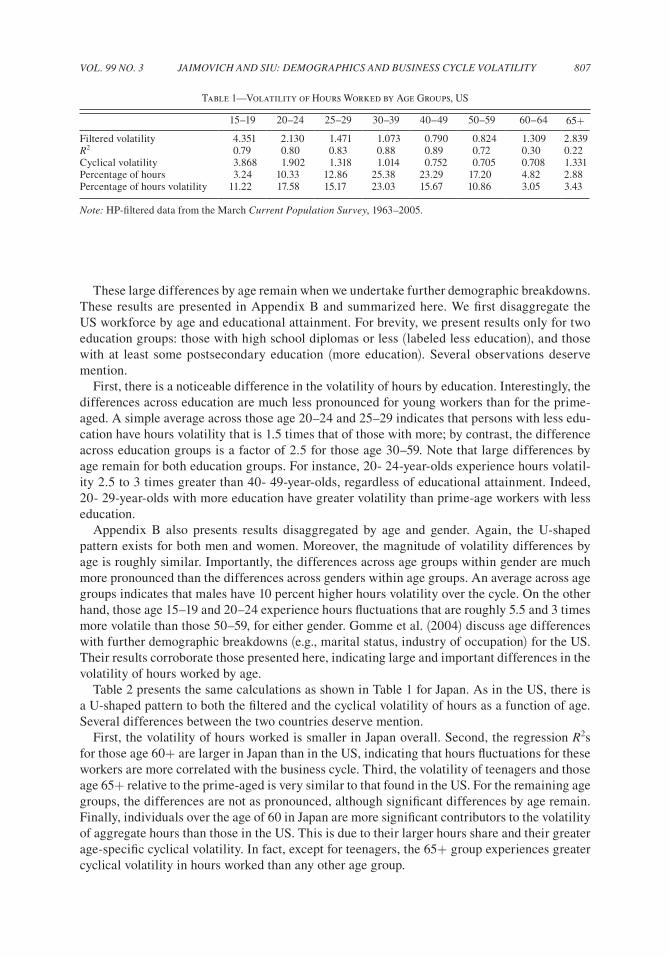
Before proceeding to the regression analysis, panels A and B of Figure 2 present time series for cyclical volatility, σi (depicted by the light lines), and the volatile-age labor force share, sharei (the dark line), for the United States and Japan. The solid light line is our benchmark “rolling window” measure of business cycle volatility; by construction, this uses HP-filtered output data from 1958 to 2004. The dashed light line is the SW measure. Both measures depict very similar pictures for the postwar evolution of cyclical volatility.

Moreover, the volatility series and the volatile-age labor force share track each other very closely in both countries. In the US, output volatility rose from the early 1960s to the late 1970s, then fell to the end of the period. This pattern is matched by our labor force measure. The hump in the labor force share that peaks around 1976 is due to the entrance of baby boomers into the workforce.

This correlation could be spurious, however, because of such factors as instability of oil prices and monetary policy in the 1970s. Our cross-country analysis provides evidence to the con-trary: in our panel regression, the effect of labor force shares is identified through differences in demographic change across countries. Consider Japan, which similarly experienced postwar moderation in output volatility and aging of the workforce, but with quite a different evolution. In contrast to the United States, Japan’s business cycle volatility fell beginning around 1970, accelerating in the late-1970s. After stabilizing in the early-1980s, volatility has since risen. Again, this pattern is closely tracked by Japan’s volatile-age labor force share. The fact that these changes in demographics and volatility represent a “mirror image” of the United States strongly suggests that the correlation is not spurious.

9 See Blanchard and Simon (2001) for a similar empirical specification, studying the relationship between inflation and output volatility.


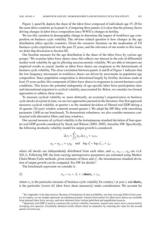
The remaining panels of Figures 2 and 3 present the same series for all G7 countries. In each panel, the scale of the vertical axes is identical to facilitate comparison. In six of the seven coun-tries, business cycle volatility and the volatile labor force share clearly covary, although there is a slight phase shift in Canada. In France, unconditional evidence of this relationship is weaker, but relative to the other countries there is little change in volatility to explain.

Table 4 presents estimation results from equation (1) on γ, the average effect of the labor force measure on business cycle volatility. Column 1 presents our OLS estimate when σit is the “rolling window” measure of the standard deviation of HP-filtered output. The regression result suffers from autocorrelated residuals. This is due in part to the construction of the volatility measure, which results in overlap of output data in consecutive observations of σit . To address this, we run standard tests on the residuals to determine the highest order of serial correlation. For this specification, we cannot reject a highest order of two. In column 1 and throughout the paper, we report results when heteroskedasticity and autocorrelation-robust standard errors are constructed using the Newey-West estimator in this manner.

The share of volatile-age workforce participants has a positive effect on business cycle vola-tility. To interpret the magnitude of the coefficient estimate, a 10 percent increase in this labor force share would increase cyclical volatility by 0.40.10 We estimate this effect to be significant at the 1 percent level.

10 Again, we delay discussion of this in relation to the US Great Moderation to the following section.

Figure 2. Demographics and Business Cycle Volatility, G7 Countries, Part 1

Notes: Dark, triangle-hatched line: volatile-age labor force share. Light, square-hatched line and light, dashed line: two measures of business cycle volatility. See text for detailed description of variables.

0.21

0.26

0.31

0.36

0.41

0.46

0.0

0.5

1.0

1.5

2.0

2.5

1963 1967 1971 1975 1979 1983 1987 1991 1995 1999

Per

cent

sta

ndar

d de

viat

ion

Panel A. US

0.22

0.27

0.32

0.37

0.42

0.47

0.0

0.5

1.0

1.5

2.0

2.5

1963 1967 1971 1975 1979 1983 1987 1991 1995 1999

Sha

re in

labo

r fo

rce

Panel B. Japan

0.22

0.27

0.32

0.37

0.42

0.47

0.0

0.5

1.0

1.5

2.0

2.5

1970 1974 1978 1982 1986 1990 1994

Year

Panel C. Germany

0.25

0.30

0.35

0.40

0.45

0.50

0.0

0.5

1.0

1.5

2.0

2.5

1966 1970 1974 1978 1982 1986 1990 1994 1998

Year

Panel D. Canada

Sha

re in

labo

r fo

rce

Per

cent

sta

ndar

d de

viat

ion

YearYear


To illustrate robustness, Table 4 reports coefficient estimates when we change the measure-ment of cyclical volatility. In column 2, we consider real output detrended by first-differencing; relative to the HP filter, this amplifies high-frequency fluctuations. This is the detrending method considered by Kim and Nelson (1999) and McConnell and Perez-Quiros (2000) in their studies of the Great Moderation. In column 3, we consider the four-quarter growth rate of real output, which is the detrending method used by SW. Next, we take the frequencies that the HP filter passes (those higher than 32 quarters), and split them approximately in two: we isolate fluctua-tions with frequency between 2 and 16 quarters and those between 17 and 32 quarters, using the band pass (BP) filter proposed by Baxter and King (1999). These results are presented in columns 4 and 5, respectively. The estimated effect of the volatile-age labor force share on all measures is positive and significant at either the 5 percent or 1 percent level. For brevity, we report only the results for the 41-quarter window; the results using a 21-quarter (5-year) window are virtually identical (see an earlier draft of this paper, Jaimovich and Siu (2007), for details). Finally, note that the magnitude of the coefficient estimates cannot be compared across columns since the definition of the dependent variable differs.

As a further experiment, we broaden our investigation by considering output fluctuations outside of the traditionally defined business cycle frequency. Specifically, Diego Comin and Mark Gertler (2006) introduce the concept of the “medium-term business cycle” to describe sustained swings across periods of growth and stagnation, in addition to the more commonly considered booms and recessions of shorter duration. Looking at the medium term allows us to include, for example, fluctuations associated with the US productivity slowdown and the onset of the Japanese stagnation

0.21

0.26

0.31

0.36

0.41

0.46

0.0

0.5

1.0

1.5

2.0

2.5

1963 1967 1971 1975 1979 1983 1987 1991 1995 1999

Per

cent

sta

ndar

d de

viat

ion

Panel A. US

0.22

0.27

0.32

0.37

0.42

0.47

0.0

0.5

1.0

1.5

2.0

2.5

1965 1969 1973 1977 1981 1985 1989 1993 1997

Panel B. France

0.22

0.27

0.32

0.37

0.42

0.47

0.0

0.5

1.0

1.5

2.0

2.5

1979 1983 1987 1991 1995 1999

Year

Panel C. UK

0.21

0.26

0.31

0.36

0.41

0.46

0.0

0.5

1.0

1.5

2.0

2.5

1983 1987 1991 1995 1999

Sha

re in

labo

r fo

rce

Year

Panel D: Italy

Per

cent

sta

ndar

d de

viat

ion

Sha

re in

labo

r fo

rce

YearYear

Figure 3. Demographics and Business Cycle Volatility, G7 Countries, Part 2

Notes: Dark, triangle-hatched line: volatile-age labor force share. Light, square-hatched line and light, dashed line: two measures of business cycle volatility. See text for detailed description of variables.


in the 1990s in our measure of volatility. To do so, we follow Comin and Gertler and isolate output fluctuations with frequency between 2 and 200 quarters using the BP filter.11 Column 6 presents the estimation result when, again, volatility is measured with a 41-quarter rolling window. We find that the volatile-age labor force share has a positive effect on medium-term cyclical volatility; however, the p-value on the estimate is 0.13, so that it falls just outside the usual range of statistical significance. We conclude that while there is evidence of an effect of demographics on medium-term volatility, it is stronger at conventional business cycle frequencies.

Finally, in column 7, we report the estimation result when σit is SW’s measure of the instan-taneous standard deviation of four-quarter real GDP growth. Again, the share of volatile-age workforce participants has a positive effect on business cycle volatility, and the effect is statisti-cally significant at the 1 percent level.

B. Further Robustness Results

The results in Table 4 are potentially subject to endogeneity problems because any group’s labor force share depends on its participation rate, which in turn may depend on (country- specific) shocks determining output volatility. Endogeneity bias results if the response of labor force par-ticipation to these shocks differs across age groups. To investigate this, we present instrumental variables (IV) results in which each country’s volatile-age labor force share is instrumented by its population share of those 15–29 and 60–64.

The first column in Table 5 repeats our benchmark OLS result from Table 4. Panel A consid-ers the rolling window measure of volatility using HP-filtered output. Column 2 presents our estimate when workforce shares are instrumented by population shares. Again, the effect of the volatile group’s labor force share is positive and significant at the 1 percent level. In fact, the estimated coefficient changes little from our OLS result. Using the Hausman test, we cannot reject the hypothesis of no endogeneity bias in our original labor force measure.

Our second IV approach goes further, addressing the possibility that the population age dis-tribution is endogenous as well. This would occur if the response of international migration to shocks determining output volatility differed across age groups. To address this, we instrument the labor force share by lagged birth rates. The motivation for this is straightforward. Excluding migration, an age group’s share of the 15- 64-year-old population is determined by the distribu-tion of births 15 to 64 years prior.12 Since past fertility is almost certainly exogenous to current

11 We implement this using the BP filter proposed by Lawrence J. Christiano and Terry J. Fitzgerald (2003). See Christiano and Fitzgerald for a discussion of the merits of their method for isolating fluctuations outside the traditional business cycle frequencies relative to that of Baxter and King (1999).

12 This ignores deaths among individuals under age 64, which is statistically negligible in G7 countries.

Table 4—Volatile-Age Labor Force Share and Business Cycle Volatility

HP FD FQ BP(hi) BP(lo) CG SW(1) (2) (3) (4) (5) (6) (7)

γ 4.022*** 2.025*** 4.647** 2.537*** 2.734** 5.464 3.339***(1.134) (0.690) (2.119) (0.697) (1.090) (3.644) (1.177)

Observations 207 207 207 180 180 207 207

Notes: Results from OLS estimation of equation (1) for different measures of the dependent variable. Newey-West stan-dard errors in parentheses.

*** Significant at the 1 percent level. ** Significant at the 5 percent level.


macroeconomic volatility, instrumenting by lagged birth rates allows us to obtain unbiased esti-mates of the causal impact of labor force composition.

We instrument by projecting the volatile-aged labor force share on 20-year, 30-year, 40-year, 50-year, and 60-year lagged birth rates. The results are presented in column 3 of Table 5. Again, the estimated effect is statistically significant at the 1 percent level, and the magnitude of the coefficient estimate is very similar to the original OLS estimate.

Using population shares and lagged birth rates as instruments is problematic, though, if demo-graphics affect cyclical volatility, independent of their influence on labor force composition. This is possible if, for example, differential demand for investment and durable goods or differential impacts of borrowing constraints across age groups have important business cycle effects. In this case, population measures may not constitute valid instruments for labor force shares.13

Given this, we consider an alternative approach to addressing the potential endogeneity of labor force measures: we simply remove the medium- and high-frequency variation in the vola-tile-age labor force share. Using the BP filter, we discard all fluctuations at frequencies greater than 20 years. This corresponds to the view that endogeneity arises from unobserved shocks, simultaneously determining labor force shares and business cycle volatility. In this case, it should suffice to restrict our attention only to low-frequency movements in workforce composition that

13 Indeed, inference on any hypothesis regarding the causal role of demographics on volatility will rely on exogenous variation in population measures. As a result, it is very difficult to provide direct evidence to exclude such alternative hypotheses. However, the results of the following subsection provide strong evidence for the labor market composition effects we emphasize.

Table 5—Volatile-Age Labor Force Share and Business Cycle Volatility: Further Robustness Checks

Endogeneity Blanchard-Simon

OLS IV1 IV2 BP OLS IV2(1) (2) (3) (4) (5) (6)

panel A: Annual, hpγ 4.022*** 3.635*** 3.946*** 4.284*** 5.430*** 5.381***

(1.134) (1.424) (1.138) (1.203) (1.095) (1.089)

panel B: Annual, SWγ 3.339*** 3.416** 3.305*** 3.575*** 4.102*** 4.076***

(1.177) (1.348) (1.185) (1.248) (1.116) (1.179)

Observations 207 207 207 207 203 203

panel c: Four-year, hpγ 4.306*** 3.411* 4.272*** 4.532*** 5.728*** 5.447***

(1.427) (1.987) (1.422) (1.596) (1.390) (1.379)

panel d: Four-year, SWγ 3.304** 3.324* 3.299* 3.479* 3.821** 3.846**

(1.660) (1.845) (1.678) (1.835) (1.613) (1.608)

Observations 55 55 55 55 53 53

Notes: Results from OLS and IV estimation of equation (1) for different measures of the dependent variable. Panels A and B use annual observations; panels C and D use observations spaced four years apart. Newey-West standard errors in parentheses.

*** Significant at the 1 percent level. ** Significant at the 5 percent level. * Significant at the 10 percent level.


are orthogonal to cyclical volatility shocks. Column 4 reports the result of this exercise. Again, the coefficient estimate is positive and significant, and is very similar to our benchmark result.

In panel B of Table 5, we repeat the preceding analysis, this time using the instantaneous volatility measure of SW as the dependent variable in equation (1). The effect of the volatile-age labor force share is positive and statistically significant at either the 5 percent or 1 percent level in all cases, and, again, we cannot reject the hypothesis of no endogeneity bias in our original labor force measure.

As a further robustness check, we add to our benchmark empirical specification the regres-sors considered by Blanchard and Simon (2001), who conclude that inflation volatility displays a strong, and potentially causal, relationship with output volatility. This conclusion is based on panel-data analysis similar to ours, in which output volatility is regressed on the mean and stan-dard deviation of inflation, along with country and time fixed effects. The inflation volatility coefficient is found to be large and statistically significant.

As Blanchard and Simon acknowledge, concern arises from the endogeneity of inflation measures and output volatility. This bias makes inference problematic. Consequently, when we include inflation measures in our analysis, we do not view the magnitude of the coefficient esti-mates as particularly informative. The point is simply to illustrate that our results are robust to concerns of spurious correlation between labor force composition and output volatility. The OLS estimate from this exercise is reported in column 5 of Table 5; column 6 reports the estimate when the labor force measure is instrumented by lagged birth rates. Including the inflation mea-sures does not alter the sign or the statistical significance of the original findings (the results for the IV1 and BP exercises are virtually identical).

Our last experiment concerns the “spacing” or temporal frequency of observations. The demo-graphic change underlying our inference is a gradual process. Consequently, meaningful varia-tion in our labor force measure obtains perhaps only at longer time horizons. This concern is addressed in panels C and D, where we repeat our analysis of panels A and B, this time with annual observations spaced four years apart.14 Panel C reports results when we use the rolling window measure of cyclical volatility, and panel D when we use the SW measure. Note that this change does not substantively affect our results, strengthening our conclusion of a positive link between the volatile group’s labor force share and output volatility.

Finally, we consider alternative definitions of the volatile-age labor force share guided by our results in Section I. In the United States, despite the fact that 60- 64-year-olds display greater volatility than those in prime age, their contribution to volatility in total hours worked is smaller than their contribution to total hours worked. The same is true in Canada, in terms of employ-ment. As such, we redefine the volatile-aged in these countries as only 15- 29-year-olds. Also, the results in Section I indicate that, unlike in other countries, in Japan those 65 and older are significant contributors to the volatility of aggregate hours and employment. Therefore, we rede-fine sharei for Japan as the fraction of the 15+ workforce accounted for by those 15–29 and 60+. Considering these changes, both separately and simultaneously, does not change any of the results reported in Tables 4 and 5. Taken together, we interpret the results of this subsection as convincing evidence of a positive effect of the labor force share of volatile-age individuals on business cycle volatility.

14 We choose this relative to a more conventional five-year spacing for practical reasons: given the unbalanced nature of our panel, this one-year drop in frequency would result in a disproportionately large drop in the number of observations.


C. Looking at the Entire Age distribution

Up to this point the results indicate that periods with a larger share of age groups with cyclically sensitive market work tend to display greater business cycle volatility. In this section, we extend our analysis to include a more detailed look at the effect of the workforce age composition.

In particular, we use the entire age distribution of the labor force as the regressor in (1). This is motivated by our results in Section I: namely, there is a U-shaped pattern in the cyclical volatil-ity of hours and employment as a function of age. Our intent is to determine whether there is a similar U-shaped effect of age shares on aggregate output volatility. This would support our view that the shape of the entire age distribution affects the responsiveness of an economy to business cycle shocks, and that the crucial channel of influence is via differences in the cyclical sensitivity of market work across age groups.

We alter our empirical specification so that the regressor, share, is a vector of labor force shares: the shares of the 30–39, 40–49, 50–59, and 60–64 age groups. Because shares sum to one, we exclude the 15- 29-year-olds for the obvious reason. This means that the coefficient on any particular age group represents the change in cyclical volatility that results from a shift of workforce share out of the 15–29 group, into that age group.

Table 6 presents results when the dependent variable is our benchmark rolling window mea-sure for HP-filtered output. Row 1 presents the OLS estimate. We include a column of zeros for the 15- 29-year-olds to reiterate the interpretation of coefficient estimates laid out in the previous paragraph. Relative to our conjecture, the estimated coefficients have the expected sign and mag-nitude. A decrease in the share of 15- 29-year-olds in favor of any other age group reduces busi-ness cycle volatility. Moreover, the effect is U-shaped as a function of age. The smallest reduction in volatility comes from shifting young workforce members into the 60–64 age group, although this effect is not significantly different from zero. This is consistent with our results in Section I, indicating that both the young and the old tend to contribute disproportionately to aggregate employment volatility in the G7. By contrast, shifting the labor force out of the young and into prime-age groups results in large and statistically significant reductions in cyclical volatility. Again, this is consistent with the U-shape in market work volatility.

We conduct additional experiments by varying the excluded age group, one at a time, from the regression. This allows us to determine the significance of differences across age-group pairs. For brevity we do not report these results, but summarize them as follows: broadly speaking, the biggest differences in volatility effects are between either the 15–29 or 60–64 age groups (Set 1)

Table 6—Labor Force Age Distribution and Business Cycle Volatility: HP

15–29 30–39 40–49 50–59 60–64 Observations

OLS 0 −3.026* −4.058*** −6.226*** −0.716 207NA (1.672) (1.489) (2.086) (4.371)

IV1 0 −3.237** −4.177*** −6.440*** −0.588 207NA (1.680) (1.485) (2.165) (4.448)

IV2 0 −2.935* −4.010*** −6.039*** −1.018 207NA (1.676) (1.500) (2.077) (4.406)

BP 0 −2.745 −4.335*** −6.769*** −0.614 207NA (1.739) (1.674) (2.520) (4.658)

Notes: Results from OLS and IV estimation of equation (1) when volatility is measured as the standard deviation of HP-filtered output within a 41-quarter window. Newey-West standard errors in parentheses.



and either the 40–49 or 50–59 age groups (Set 2). Across Set 1 and Set 2, the difference in coeffi-cient estimates for any pair of age groups is large and statistically significant. On the other hand, for pairs within Sets 1 and 2, the estimated difference is small and insignificant. The 30- 39-year-olds represent an intermediate group. When this group is excluded, the coefficient is statistically significant at the 1 percent and 10 percent levels for the 50–59s and 15–29s, respectively, and is insignificant for the 40–49s and 60–64s.15

In the remaining rows of Table 6 we report robustness checks that address the potential endo-geneity of labor force shares. In row 2 we present IV estimates using population shares as instru-ments; in row 3 we present IV estimates using lagged birth rates (see the previous subsection for details). The results are hardly changed relative to row 1. Row 4 presents the results when we BP filter the workforce shares to retain only fluctuations with periodicity greater than 20 years, as described in the previous subsection. Again, the effect on business cycle volatility is U-shaped as a function of age.

Table 7 presents the same regression estimates as Table 6, but using SW’s instantaneous vola-tility measure. Again, a decrease in the share of 15- 29-year-olds in favor of any other age group reduces cyclical volatility. The largest effect comes from shifting young workforce members into the 40–49 age group, where the reduction is estimated to be significant at either the 5 percent or 1 percent level. As in Table 6, shifting the labor force out of the young and into the 60–64 age group does not result in a statistically significant volatility reduction. As such, the effect can again be characterized as U-shaped as a function of age.

To determine robustness, we repeat our analysis of the workforce age distribution by using observations spaced four years apart. Though not reported here, statistically significant age group effects and a U-shaped pattern in coefficient estimates as a function of age were found (see Jaimovich and Siu 2007 for details). Finally, we include measures of average inflation and infla-tion volatility in our analysis. Again, our results regarding the sign and statistical significance of the coefficient estimates are unchanged.

15 Though the results are not reported here, we also experiment using different splits in age groups to ensure robust-ness. For instance, we split the young into two groups, those age 15–24 and those age 25–29. This has minimal impact on the results. Again, we obtain a U-shaped impact of workforce age shares on cyclical volatility. In fact, we find no significant difference between the estimated effect of the 15–24 and 25–29 groups. Other splits yield similar results, and maintain the U-shaped pattern.

Table 7—Labor Force Age Distribution and Business Cycle Volatility: SW

15–29 30–39 40–49 50–59 60–64 Observations

OLS 0 −2.873* −4.133*** −2.775* −3.806 207NA (1.714) (1.548) (1.663) (4.053)

IV1 0 −3.045* −4.289*** −3.078 −3.032 207NA (1.714) (1.533) (1.940) (4.239)

IV2 0 −2.949* −4.027*** −2.787 −3.811 207NA (1.743) (1.570) (1.881) (4.166)

BP 0 −2.913 −4.319** −3.506 −3.689 207NA (1.892) (1.727) (2.407) (4.528)

Notes: Results from OLS and IV estimation of equation (1) when volatility is measured as the instantaneous standard deviation of output growth. Newey-West standard errors in parentheses.



Given the U-shaped pattern documented in Section I, we view this as compelling evidence that the influence of demographic composition on volatility operates through differences in the cycli-cal sensitivity of hours and employment across age groups. The pattern of market work volatility as a function of age represents a natural explanation for the U-shaped impact of age shares on business cycle volatility. Indeed, any other hypothesis regarding the impact of demographic com-position on output volatility would need to rationalize this pattern.

D. A Joint Estimation procedure

As a final exercise, we pursue an approach that allows us to jointly obtain estimates of time-varying business cycle volatility and the role of the workforce age distribution in its determina-tion. As a by-product, this allows us to avoid such issues as those associated with serial correlation of residuals in (1) from the use of rolling windows in measuring volatility.

Specifically, we follow the methodology of Garey Ramey and Valerie A. Ramey (1995), who used a similar approach to analyze the effect of government spending–induced volatility on economic growth.16 For our purposes, we consider the following empirical framework linking demographics to the volatility of real output growth:

(2) Δ yit = μi + υit ,

(3) υit ~ N(0, σ2it), σit = αi + βt + γ shareit.

Here, Δ yit is output growth for country i in period t, μi is mean growth in country i, σit is the time-varying standard deviation of the residual υit , and shareit is the labor force age composition measure under consideration. We estimate the system (2)–(3) using full information maximum likelihood.

Table 8 presents the results from this procedure. Column 1 presents the coefficient estimate of γ when share is the volatile-age labor force share. The coefficient is positive and statistically significant at the 1 percent level. The remaining columns present the results when the regressor is the vector of 30–39, 40–49, 50–59, and 60–64 group labor force shares. Again, we obtain sta-tistically significant reductions in output growth volatility by shifting workforce share out of the

16 We thank one of the anonymous referees for suggesting this to us.

Table 8—Joint Estimation of Volatility and Effect of Demographics

Volatile-age 15–29 30–39 40–49 50–59 60–64(1) (2) (3) (4) (5) (6)

γ 4.476*** 0 −5.939*** −4.337*** −6.103*** −2.650(1.243) NA (1.777) (1.443) (2.033) (4.883)

Observationsa 807 807

Notes: Results from FIML estimation of system (2)–(3). Standard errors in parentheses.*** Significant at the 1 percent level.aDue to problems with convergence, the model was estimated at the quarterly frequency, using one time dummy, βt,

for every two adjacent quarters.


young and into the prime-age groups. As before, shifting the labor force out of the 15–29 group and into the 60–64 group does not result in a statistically significant volatility reduction.

To summarize, we find convincing evidence that the workforce age composition is a key determinant of an economy’s responsiveness to business cycle shocks. Estimation results from our benchmark specification, (1), and the system, (2)–(3), indicate that there is a large and sta-tistically significant effect of the labor force age distribution on cyclical volatility. Moreover, the largest effect comes from shifting the workforce across young and prime-age demographic groups, those with the largest difference in the volatility of hours and employment over the busi-ness cycle.

III. The Great Moderation: Quantitative Accounting

Since the mid-1980s the United States has undergone a substantial decline in business cycle volatility, as shown in Figure 2, panel A. Indeed, determining the causes of the Great Moderation is the objective of a growing body of literature. Potential explanations include a reduction in inflation volatility that is potentially related to improved monetary policy (see, for instance, Richard Clarida, Jordi Galí, and Gertler 2000; Blanchard and Simon 2001; Stock and Watson 2003); regulatory changes and financial market innovation related to household borrowing (Jeffrey R. Campbell and Zvi Hercowitz 2005; Jonas D. M. Fisher and Martin Gervais 2007; Alejandro Justiniano and Giorgio E. Primiceri 2008), changes that have reduced the volatility of production relative to sales (McConnell and Perez-Quiros 2000; Ramey and Daniel J. Vine 2006); and good luck, in the form of a reduction in the variance of business cycle shocks (Stock and Watson 2003, 2005; Justiniano and Primiceri 2008; Andres Arias, Gary Hansen, and Lee Ohanian 2007).

In this section, we take a first step at quantifying the role of demographic change in accounting for the Great Moderation. In other work, we consider a quantitative theoretical approach which takes a specific stance on the impulses generating cyclical fluctuations and the effect of demo-graphic change on the propagation of shocks (see Jaimovich, Seth Pruitt, and Siu 2008). We view the simple accounting exercises conducted here as suggestive of the magnitude in change owing to demographic considerations, and indicative of the need to pursue careful quantitative analysis.

Our first exercise simply involves interpreting the coefficient estimates from our G7 panel regression, (1). Consider first the standard deviation of HP-filtered output calculated over a roll-ing ten-year time window; this is plotted as the light, solid line in Figure 2, panel A. According to this measure, US business cycle volatility peaks in 1978. This year corresponds with a 15- 29-year-old labor force share of 39.7 percent. Volatility then falls during the 1980s, coinciding with an aging of the workforce as baby boomers enter their prime-age years. By 1999, the 15- 29-year-old share is only 27.9 percent, representing a level reduction of 11.8 percent from 1978.

From our OLS estimates in Table 6, it follows that such a shift in workforce composi-tion—from the 15–29 age group into the 40–49 age group—predicts a volatility reduction of 0.118 × 4.058 = 0.479. Given that our measure of cyclical volatility falls from 2.379 to 0.955 between 1978 and 1999, this change in age composition accounts for roughly 34 percent of the moderation between these two dates.

The light, dashed line in Figure 2 depicts Stock and Watson’s (2003, 2005) instantaneous standard deviation of output growth. This volatility measure peaks in 1981 before falling during the mid-1980s. Performing the same exercise as above, we find that the change in workforce age composition accounts for roughly 35 percent of the moderation in this measure.

Finally, we present a simple decomposition exercise to determine how much of the change in aggregate market work volatility is attributable to the change in the age distribution of the work-force. We use the data analyzed in Section I and compare the volatility of HP-filtered measures across 1967–1984 and 1985–2004.


The standard deviation of per capita aggregate employment fluctuations falls 62.2 log points across the two periods. To isolate the effect due purely to the change in composition, we con-struct a counterfactual series for per capita aggregate employment, et, that holds the age structure fixed. Note that

et = et15 pt

15 + et20 pt

20 + … + et65 pt

65,

where et15 is per capita employment (or the employment rate) of 15- 19-year-olds, et

20 is the employment rate of 20- 24-year-olds, and so on, progressing in 5-year age groups; et

65 is the employment rate of those 65 and older at date t, and pt

x is the population share of age group x. The counterfactual series are constructed using the observed age-specific employment rates, {et

x }, but setting the population shares constant. Our exercise holds the age composition fixed at the average values during the premoderation (1967–1984) period, so that counterfactual aggregate employment for date t is

etpre = et

15 p15pre + et

20 p20pre + … + et

65 p65pre .

Doing this for every year, 1967–2004, generates a counterfactual time series {etpre}.

We compare the standard deviation of filtered counterfactual employment across the pre- and postmoderation periods. Had the age composition stayed constant at the average premoderation level, the standard deviation would have fallen by only 47.2 log points. That is, the change in age composition explains (62.2 − 47.2) ÷ 62.2 or 24 percent of the moderation in aggregate employ-ment volatility. Performing the same experiment for hours worked, we find that 20 percent of its moderation is due to demographic change.

Is this decomposition exercise informative? Note that the experiment assumes that the volatil-ity of age-specific market work is independent of the age composition. That is, it assumes the absence of indirect effects of changing age structure on aggregate volatility via changes in the volatility of age-specific employment and hours worked.

To determine whether this is reasonable, we test for the presence of such effects using cross-country regression analysis similar to that considered in Section II. For example, we regress the volatility of employment of 15- 29-year-olds on the 15- 29-year-old labor force share, controlling for country fixed effects and factors affecting business cycle volatility common across countries. We find that a 10 percent increase in the share of 15- 29-year-olds decreases the standard devia-tion of their employment by 0.0007 percent; this is not estimated to be different from zero at conventional significance levels. For brevity, we do not report results for other age groups since, again, the effects are estimated to be small in magnitude and statistically insignificant. Hence, we find no strong evidence for these indirect effects in the G7 sample.

To get a sense of the importance of the age composition effect, we performed the same decomposition for other demographic factors. As discussed in Section I, differences exist in the cyclical volatility of hours worked for those with high school diplomas or less, relative to those with at least some postsecondary education. Running a counterfactual where we hold the education composition fixed at the average 1967–1984 level, we find that rising educational attainment in the United States accounts for roughly 10 percent of the observed reduction in aggregate hours volatility. This compares to the value of 20 percent reported above from hold-ing the age composition fixed, and a value of 29 percent when we simultaneously hold the age-and-education composition fixed.

Likewise, we considered experiments on the gender composition of the workforce. Holding the male-female shares constant at the premoderation levels resulted in essentially no change in the volatility of aggregate hours. Similarly, holding the gender-and-age or gender-age-and-education


composition constant produced negligible differences from simply holding the age or age-and-education composition fixed, as reported in the previous paragraph.

As a result, we find age composition change as the single most important demographic fac-tor in the reduction of market work volatility. Moreover, because this demographic change was driven by the baby boom of the 1950s, it is much easier to establish exogeneity with respect to the moderation of the 1980s. This is in contrast to the compositional changes due to trends in post-secondary enrollment and female labor force participation decisions. Finally, the hump-shaped change induced by the baby boom generates a relationship with both the run-up in volatility of the late-1960s and the recent moderation. The steady trends in educational attainment and labor force participation have less predictive power with respect to the nonmonotonic change observed in the United States.

To conclude, note that the results of the decomposition exercise on aggregate market work vol-atility are similar in magnitude to the role of age composition change in the moderation of output volatility derived from our panel regression analysis. We take this as evidence of an important role for demographics in explaining the Great Moderation.

IV. Conclusion

Recent work has documented the empirical implications of demographic change for mac-roeconomic analysis.17 In this paper, we investigate the consequences of demographic change for business cycle analysis. We find that changes in the age composition of the labor force account for a significant fraction of the variation in postwar business cycle volatility in G7 economies.

Our identification comes from variation in the nature and timing of demographic change expe-rienced across countries during the postwar period. Using panel data methods, we show that the age composition of the workforce has a quantitatively large and statistically significant effect on cyclical volatility. Moreover, the estimated effect is found to be U-shaped as a function of age. We supplement this by documenting a U-shaped pattern in the cyclical volatility of employment and hours worked across age groups in the same sample of countries. Taken together, these findings suggest that the channel of influence of demographic composition on business cycle volatility operates through differences in the sensitivity of market work across age groups. Finally, through a series of quantitative accounting exercises, we find that age composition change accounts for roughly one-fifth to one-third of the moderation in cyclical volatility experienced in the United States.

These results indicate that the demographic composition of an economy’s workforce consti-tutes a potentially important propagation mechanism in business cycle analysis. As such, there are strong returns to a theoretical understanding for why differences in cyclical volatility of market work exist across age groups, and how variation in the workforce age composition mani-fests itself in variation of macroeconomic volatility.18

In Jaimovich, Pruitt, and Siu (2008), we address these issues within the context of a quan-titative macroeconomic model featuring capital-experience complementarity in production. We show that the model is capable of matching observed differences in the cyclicality of both hours worked and real wages across age groups. Moreover, we demonstrate that variation in the

17 See, for instance, Robert Shimer (1998) and Katharine G. Abraham and Shimer (2001) who study the impact of the aging of the baby boom population on US unemployment, and James Feyrer (2007) on the relationship between workforce age composition and productivity growth.

18 Indeed, an interesting question is whether such an explanation can also address the results of Shimer (1998) and Abraham and Shimer (2001) regarding demographic composition and average unemployment.


age composition of aggregate hours accounts for a significant fraction of the moderation in US business cycle volatility observed in the past 25 years. These results corroborate estimates of the role of demographics in the Great Moderation that are derived from our simple quantitative exercises presented here. In summary, we conclude that demographic composition constitutes an important propagation mechanism in business cycle analysis, and an important factor in under-standing the evolution of postwar business cycle volatility.

Appendix A: Data Sources

United States. Hours worked: 1963–2005, March CPS, Bureau of Labor Statistics, and US Census Bureau. Employment, labor force, and population: 1963–2004, OECD Labour Force Statistics database (hereafter OECD LFS). Birth rates: 1900–1989, historical Statistics of the United States, colonial times to 1970, and Mini Historical Statistics, US Census Bureau. Real GDP: 1958–2004, FRED database, Federal Reserve Bank of St. Louis.

Japan. Hours worked: 1972–2004, Annual Report of the Labour Force Survey (hereafter ARLFS), Statistics Bureau of Japan. Employment: 1967–1971, OECD LFS; 1972–2004, ARLFS. Labor force and population: 1963–1971, OECD LFS; 1972–2004, ARLFS. Birth rates: 1900–1989, historical Statistics of Japan, Statistics Bureau of Japan. Real GDP: 1958–2004, Economic and Social Research Institute, Cabinet Office, Government of Japan.

Canada: Employment: 1976–2004, OECD LFS. Labor force and population: 1966–1975, spe-cial tabulation of Labour Force Survey provided by Statistics Canada; 1976–2004, OECD LFS. Birth rates: 1900–1989, Brian R. Mitchell (2003b). Real GDP: 1961–2004, CANSIM database.

France: Employment: 1968–2004, OECD LFS. Labor force and population: 1965–2004, OECD LFS. Birth rates: 1900–1989, Mitchell (2003a). Real GDP: 1960–2002, Stock and Watson (2003), which has been modified to account for 1968 strikes.

Germany: Employment, labor force and population: 1970–2004, OECD LFS. Birth rates: 1900–1955, Mitchell (2003a); 1956–1989, Federal Statistics Office, Germany. Real GDP: 1965–2002, Stock and Watson (2003), which has been modified to account for 1991 reunification.

Italy: Employment and labor force: 1983–2004, Eurostat database and OECD LFS. Population: 1983–2004, World population prospects, United Nations. Birth rates: 1900–1989, Mitchell (2003a). Real GDP: 1978–2004, Stock and Watson (2003), and Eurostat database.

UK: Employment: 1983, special tabulation of Labour Force Survey provided by Office for National Statistics, UK; 1984–2004, OECD LFS. Labor force and population: 1979–1983, spe-cial tabulation of Labour Force Survey provided by Office for National Statistics, UK; 1984–2004, OECD LFS. Birth rates: 1900–1989, Mitchell (2003a). Real GDP: 1974–2004, Office for National Statistics, UK.

For all countries, inflation rates constructed from GDP deflator data obtained from the Datastream database, Thomson Financial.

Appendix B: Further Demographic Splits of Hours Worked

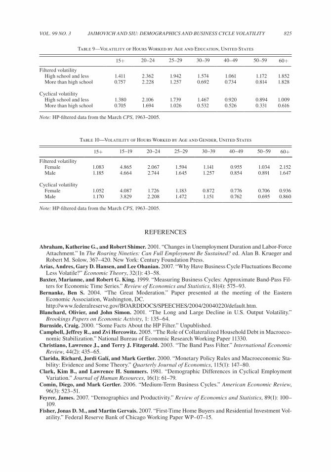
In Table 9 we present results on the volatility of hours worked in the United States by age and education. Because of the relatively small fraction of 15- 19-year-olds with postsecondary educa-tion, we omit them in the analysis; because of smaller sample sizes, we combine the 60–64 and 651 age groups.

Table 10 presents the volatility of hours worked in the United States by age and gender. Again, because of smaller sample sizes, we combine the 60–64 and 651 age groups.


REFERENCES

Abraham, Katherine G., and Robert Shimer. 2001. “Changes in Unemployment Duration and Labor-Force Attachment.” In the Roaring Nineties: can Full Employment Be Sustained? ed. Alan B. Krueger and Robert M. Solow, 367–420. New York: Century Foundation Press.

Arias, Andres, Gary D. Hansen, and Lee Ohanian. 2007. “Why Have Business Cycle Fluctuations Become Less Volatile?” Economic theory, 32(1): 43–58.

Baxter, Marianne, and Robert G. King. 1999. “Measuring Business Cycles: Approximate Band-Pass Fil-ters for Economic Time Series.” Review of Economics and Statistics, 81(4): 575–93.

Bernanke, Ben S. 2004. “The Great Moderation.” Paper presented at the meeting of the Eastern Economic Association, Washington, DC. http://www.federalreserve.gov/BOARDDOCS/SPEECHES/2004/20040220/default.htm.

Blanchard, Olivier, and John Simon. 2001. “The Long and Large Decline in U.S. Output Volatility.” Brookings papers on Economic Activity, 1: 135–64.

Burnside, Craig. 2000. “Some Facts About the HP Filter.” Unpublished.Campbell, Jeffrey R., and Zvi Hercowitz. 2005. “The Role of Collateralized Household Debt in Macroeco-

nomic Stabilization.” National Bureau of Economic Research Working Paper 11330.Christiano, Lawrence J., and Terry J. Fitzgerald. 2003. “The Band Pass Filter.” International Economic

Review, 44(2): 435–65.Clarida, Richard, Jordi Galí, and Mark Gertler. 2000. “Monetary Policy Rules and Macroeconomic Sta-

bility: Evidence and Some Theory.” Quarterly Journal of Economics, 115(1): 147–80.Clark, Kim B., and Lawrence H. Summers. 1981. “Demographic Differences in Cyclical Employment

Variation.” Journal of human Resources, 16(1): 61–79.Comin, Diego, and Mark Gertler. 2006. “Medium-Term Business Cycles.” American Economic Review,

96(3): 523–51.Feyrer, James. 2007. “Demographics and Productivity.” Review of Economics and Statistics, 89(1): 100–

109.Fisher, Jonas D. M., and Martin Gervais. 2007. “First-Time Home Buyers and Residential Investment Vol-

atility.” Federal Reserve Bank of Chicago Working Paper WP–07–15.

Table 10—Volatility of Hours Worked by Age and Gender, United States

15+ 15–19 20–24 25–29 30–39 40–49 50–59 60+

Filtered volatility Female 1.083 4.865 2.067 1.594 1.141 0.955 1.034 2.152 Male 1.185 4.664 2.744 1.645 1.257 0.854 0.891 1.647

Cyclical volatility Female 1.052 4.087 1.726 1.183 0.872 0.776 0.706 0.936 Male 1.170 3.829 2.208 1.472 1.151 0.762 0.695 0.860

Note: HP-filtered data from the March cpS, 1963–2005.

Table 9—Volatility of Hours Worked by Age and Education, United States

15+ 20–24 25–29 30–39 40–49 50–59 60+

Filtered volatility High school and less 1.411 2.362 1.942 1.574 1.061 1.172 1.852 More than high school 0.757 2.228 1.257 0.692 0.734 0.814 1.828

Cyclical volatility High school and less 1.380 2.106 1.739 1.467 0.920 0.894 1.009 More than high school 0.705 1.694 1.026 0.532 0.526 0.331 0.616

Note: HP-filtered data from the March cpS, 1963–2005.


Gomme, Paul, Richard Rogerson, Peter Rupert, and Randall Wright. 2005. “The Business Cycle and the Life Cycle.” In National Bureau of Economic Research macroeconomics Annual 2004. Vol. 19, ed. Mark Gertler and Kenneth Rogoff, 415–61. Cambridge, MA: MIT Press.

Hoynes, Hilary W. 2000. “The Employment, Earnings, and Income of Less Skilled Workers over the Busi-ness Cycle.” In Finding Jobs: Work and Welfare Reform, ed. David E. Card and Rebecca M. Blank, 23–71. New York: Russell Sage Foundation.

Jaimovich, Nir, and Henry E. Siu. 2007. “The Young, the Old, and the Restless: Demographics and Busi-ness Cycle Volatility.” Federal Reserve Bank of Minneapolis Staff Report 387.

Jaimovich, Nir, Seth Pruitt, and Henry E. Siu. 2008. “The Demand for Youth: Implications for the Hours Volatility Puzzle and the Great Moderation.” http://www.econ.ubc.ca/siu/research/jps200811.pdf.

Justiniano, Alejandro, and Giorgio E. Primiceri. 2008. “The Time-Varying Volatility of Macroeconomic Fluctuations.” American Economic Review, 98(3): 604–41.

Kim, Chang-Jin, and Charles R. Nelson. 1999. “Has the U.S. Economy Become More Stable? A Bayes-ian Approach Based on a Markov-Switching Model of the Business Cycle.” Review of Economics and Statistics, 81(4): 608–16.

Kydland, Finn E., and Edward C. Prescott. 1993. “Cyclical Movements of the Labor Input and Its Implicit Real Wage.” Economic Review, 29(2): 12–23.

McConnell, Margaret M., and Gabriel Perez-Quiros. 2000. “Output Fluctuations in the United States: What Has Changed since the Early 1980’s?” American Economic Review, 90(5): 1464–76.

Mitchell, Brian R. 2003a. International historical Statistics: Europe, 1754–2000. New York: Palgrave Macmillan.

Mitchell, Brian R. 2003b. International historical Statistics: the Americas, 1750–2000. New York: Pal-grave Macmillan.

Moser, James W. 1986. “Demographic and Time Patterns in Layoffs and Quits.” Journal of human Resources, 21(2): 178–99.

Nagypál, Éva. 2005. “The Business Cycle and the Life Cycle: Comment.” In National Bureau of Economic Research macroeconomics Annual 2004. Vol. 19, ed. Mark Gertler and Kenneth Rogoff, 462–77. Cam-bridge, MA: MIT Press.

Ramey, Garey, and Valerie A. Ramey. 1995. “Cross-Country Evidence on the Link between Volatility and Growth.” American Economic Review, 85(5): 1138–51.

Ramey, Valerie A., and Daniel J. Vine. 2006. “Declining Volatility in the U.S. Automobile Industry.” American Economic Review, 96(5): 1876–89.

Ravn, Morten O., and Harald Uhlig. 2002. “On Adjusting the Hodrick-Prescott Filter for the Frequency of Observations.” Review of Economics and Statistics, 84(2): 371–76.

Ríos-Rull, José-Víctor. 1996. “Life-Cycle Economies and Aggregate Fluctuations.” Review of Economic Studies, 63(3): 465–89.

Shimer, Robert. 1999. “Why Is the U.S. Unemployment Rate So Much Lower?” In National Bureau of Economic Research macroeconomics Annual 1998. Vol. 13, ed. Ben S. Bernanke and Julio J. Rotem-berg, 11–61. Cambridge, MA: MIT Press.

Stock, James H., and Mark W. Watson. 2003. “Has the Business Cycle Changed and Why?” In National Bureau of Economic Research macroeconomics Annual 2004. Vol. 19, ed. Mark Gertler and Kenneth Rogoff, 159–218. Cambridge, MA: MIT Press.

Stock, James H., and Mark W. Watson. 2005. “Understanding Changes in International Business Cycle Dynamics.” Journal of the European Economic Association, 3(5): 968–1006.

Documents

The Young, the Old, and the Restless: Demographics and Business