The Yield Curve as a Leading Indicator

8/3/2019 The Yield Curve as a Leading Indicator

http://slidepdf.com/reader/full/the-yield-curve-as-a-leading-indicator 1/8

The Yield Curve as a Leading Indicator: Some Practical Issues

Arturo Estrella and Mary R. Trubin

Since the 1980s, economists have argued that the slope of the yield curve—the spread between

long- and short-term interest rates—is a good predictor of future economic activity. While much

of the existing research has documented how consistently movements in the curve have signaled

past recessions, considerably less attention has been paid to the use of the yield curve as a forecasting

tool in real time. This analysis seeks to fill that gap by offering practical guidelines on how best

to construct the yield curve indicator and to interpret the measure in real time.

B efore each of the last six recessions, short-

term interest rates rose above long-termrates, reversing the customary pattern and

producing what economists call a yield curve inversion. Thus,it is not surprising that the recent flattening of the yield curvehas attracted the attention of the media and financial mar-kets and prompted speculation about the possibility of a newdownturn. Since the 1980s, an extensive literature has devel-oped in support of the yield curve as a reliable predictor of

recessions and future economic activity more generally.Indeed, studies have linked the slope of the yield curve tosubsequent changes in GDP, consumption, industrial produc-tion, and investment.

Whereas most earlier analysis has focused on documentinghistorical relationships,the use of the yield curve as a forecastingdevice in real time raises a number of practical issues that havenot been clearly settled in the scholarly literature. First, the lackof a single accepted explanation for the relationship between theyield curve and recessions has led some observers to questionwhether the yield curve can function practically as a leadingindicator. If economists cannot agree on why the relationshipexists, confidence in this indicator may be weakened. Second,

the literature lacks a standard approach to constructing fore-casts based on movements in the yield curve. How should the

slope of the yield curve be defined? What measure of economicactivity should be used to assess the yield curve’s predictivepower? The current variety of approaches to producing andinterpreting yield curve forecasts may lead to misreadings of thesignal in real time.

This edition of Current Issues undertakes to shed light onsome of the practical problems arising from the use of theyield curve as a forecasting tool. We begin by consideringwhether there are explanations of the yield curve’s predictivepower that would justify the operational use of this signal. Wethen discuss how best to construct the yield curve indicator

and subsequently interpret the measure in real time. Ouranalysis offers specific guidelines on the choice of interestrates used to calculate the spread, the definition of recessionsused in the forecasts, and the strength and duration requiredof the yield curve signals.

Conceptual ConsiderationsThe literature on the use of the yield curve to predict recessionshas been predominantly empirical, documenting correlationsrather than building theories to explain such correlations. Thisfocus on the empirical may have created the unfortunateimpression that no good explanation for the relationshipexists—in other words, that the relationship is a fluke. In fact,

C urrent I ssuesC urrent I ssuesI N E C O N O M I C S A N D F I N A N C

Volume 12, Number 5 July/August 2006

F E D E R A L R E S E R V E B A N K O F N E W Y O R Kw w w . n e w y o r k f e d . o r g / r e s e a r c h / c u r r e n t _ i s s u e s

w w w . n e w y o r k f e d . o r g / r e s e a r c h / c u r r e n t _ i s s u e s



C U R RE NT I S S UE S I N E CO NO MI CS A ND F IN AN CE V O L U M E 1 2 , N U M B E R 5

there is no shortage of reasonable explanations, many of whichdate back to the early literature on this topic and have now beenextended in various directions. For the most part, these explana-tions are mutually compatible and, viewed in their totality,suggest

that the relationships between the yield curve and recessions arelikely to be very robust indeed.We give two examples that empha-size monetary policy and investor expectations,respectively.1

Monetary policy can influence the slope of the yield curve.A

tightening of monetary policy usually means a rise in short-terminterest rates,typically intended to lead to a reduction in inflation-ary pressures. When those pressures subside, it is expected that apolicy easing—lower rates—will follow. Whereas short-terminterest rates are relatively high as a result of the tightening, long-term rates tend to reflect longer term expectations and rise by lessthan short-term rates.The monetary tightening both slows downthe economy and flattens (or even inverts) the yield curve.

Changes in investor expectations can also change the slope

of the yield curve. Consider that expectations of future short-term interest rates are related to future real demand for creditand to future inflation. A rise in short-term interest rates

induced by monetary policy could be expected to lead to afuture slowdown in real economic activity and demand forcredit, putting downward pressure on future real interest rates.At the same time, slowing activity may result in lower expectedinflation, increasing the likelihood of a future easing in mone-tary policy. The expected declines in short-term rates wouldtend to reduce current long-term rates and flatten the yieldcurve. Clearly, this scenario is consistent with the observed cor-relation between the yield curve and recessions.

The multiplicity of channels through which the predictivepower of the yield curve may manifest itself makes it difficult togive one simple explanation for that power.However,it also sug-gests a certain robustness to the relationship between the yield

curve and economic activity: if one channel is not in play at anyone time, other channels may take up the slack.

The conceptual relationships outlined here also have implica-tions for the signals provided by the yield curve indicator.First,the

fact that long-term investor expectat ions f igure so importantlyin these relationships means that the yield curve may be moreforward-looking than other leading indicators.In other words,therecession signals produced by the yield curve may come signifi-

cantly in advance of those produced by other indicators.2

Second, the signals provided by the yield curve may be verysensitive to changes in financial market conditions. The precise

effect of these changes on the yield curve will depend onwhether they stem from technical factors or economic funda-mentals. For example, because different maturities of fixed-income securities appeal to different clienteles, a permanent

shift in the relative importance of clienteles could produce per-manent shifts in the slope of the yield curve.Alternatively, a tem-porary change in the demand for assets of a given maturity—say, a change resulting from hedging activities—could affect theslope of the yield curve for a short time before the yield curvereturns to values determined by economic fundamentals. Theseconsiderations suggest that the signals produced by the yieldcurve must show some degree of persistence if they are to be

meaningful, an issue to which we return below.

Empirical ConsiderationsTo make the best possible use of the predictive power of theyield curve, it is important to validate the predictive procedurehistorically and to apply it consistently in real time. In this sec-tion, we consider the elements of one such approach, a model inwhich a measure of the steepness of the yield curve is used topredict subsequent recessions.

The Probability Model

Empirically, we would like to construct a model that translatesthe steepness of the yield curve at the present time into a likeli-hood of a recession some time in the future. Thus, we need to

identify three components: a measure of steepness, a definitionof recession, and a model that connects the two. The approachwe employ is a “probit” equation, which uses the normal distri-bution to convert—in our application—the value of a measure

of yield curve steepness into a probability of recession one yearahead. Details of this calculation are given in the box.

The input to this calculation is the value of the term spread,that is, the difference between long- and short-term interestrates in month t . The output is the probability of a recessionoccurring in month t+12 from the viewpoint of informationavailable in month t . Both of these variables, however, need tobe defined more precisely—that is, we need to specify what we

mean by a recession and which long- and short-term interestrates we will use to produce the spread that constitutes ourmeasure of steepness.

Defining RecessionsThe standard dating of U.S. recessions derives from the cyclical

peaks and troughs identified by the National Bureau of EconomicResearch (NBER). To convert the NBER monthly dates into amonthly recession indicator, we classify as a recession everymonth between the peak and the subsequent trough, as well asthe trough itself. The peak is not classified as a recession monthbecause the economy would have grown from the previousmonth.A similar rule may be applied to the NBER quarterly datesto derive a quarterly recession indicator. These conventions,while

2

1For more detailed explanations and theoretical models, see Harvey (1988),Estrella and Hardouvelis (1991), Eijffinger, Schaling, and Verhagen (2000),Rendu de Lint and Stolin (2003), Hardouvelis and Malliaropulos (2004), andEstrella (2005).

2See,for example,Estrella and Mishkin (1996).



w w w . n e w y o r k f e d . o r g / r e s e a r c h / c u r r e n t _ i s s u e s 3

not the only possible ones, are the most frequently used inresearch on U.S.recessions.3

Measuring the Spread

The interest rates used to compute the spread between long-term and short-term rates vary across the literature on the yieldcurve’s predictive power. For example, market analysts oftenchoose to focus on the difference between the ten-year and two-

year Treasury rates, while some academic researchers havefavored the spread between the ten-year Treasury rate and thefederal funds rate. Other rates explored in the literature vary asto maturity, obligor, and computational basis. In choosing themost appropriate rates, one should consider a number of crite-

ria, including the ready availability of historical data and consis-tency in the computation of rates over time. It is also importantto consider the role of risk premiums and coupons, although at

present there is no standard way of dealing with these issues.

The criteria cited allow us to rule out some interest rates as a

measure of yield curve steepness. While a yield curve may be

constructed from Eurodollar, swap, or corporate rates, all three

have important drawbacks: comprehensive historical data on

the rates are lacking and the number of points they provide

along the yield curve is limited.By contrast, Treasury rates readily meet our criteria for the

yield curve indicator. Data since the 1950s are available for sev-

eral maturities, and are consistently computed over the entire

period. Treasury securities are also useful because they are not

subject to significant credit risk premiums that, at least in prin-

ciple, may change with maturity and over time. Pairing the

long-term Treasury rate with the federal funds rate as the

short-term rate is a possibility, but while the spread between

ten-year Treasuries and fed funds has been a very accurate pre-

dictor of U.S. recessions during some time periods, it has been

less so in others.

If Treasury rates are the best choice for our yield curve indi-cator,then we must next determine what maturity combination

works most effectively. In forecasts of real activity, the most

accurate results are obtained by taking the difference between

two Treasury yields whose maturities are far apart. At the long

end of the curve, the clear choice seems to be a ten-year rate,

the longest maturity available in the United States on a consis-

tent basis over a long sample period. We use the ten-year con-

stant maturity rate from the H.15 statistical release (“Selected

Interest Rates”) issued by the Board of Governors of the Federal

Reserve System.

With regard to the short-term rate, earlier research suggeststhat the three-month Treasury rate, when used in conjunction

with the ten-year Treasury rate, provides a reasonable combina-

tion of accuracy and robustness in predicting U.S. recessions over

long periods. Maximum accuracy and predictive power are

obtained with the secondary market three-month rate expressed

on a bond-equivalent basis,4 rather than the constant maturity

rate,which is interpolated from the daily yield curve for Treasury

securities.5

Spreads based on any of the rates mentioned are highly cor-related with one another and may be used to predict recessions.Note, however, that the spreads may turn negative—that is, the

yield curve may invert—at different points and with differentfrequencies. For instance, the ten-year minus two-year spread

3Other conventions may lead to different results. For example, Estrella,Rodrigues, and Schich (2003) and Wright (2006) use a “cumulative” recessionindicator that identifies a recession occurring in any of the following severalquarters, and Wright (2006) classifies peaks as recession periods.

4The H.15 release provides the secondary market rate on a discount basis.To con-vert the three-month discount rate to a bond-equivalent basis,we apply the trans-formation: bond-equivalent = 100*(365*discount/100)/(360-91*discount/100),where “discount”is the discount yield expressed in percentage points.

5A drawback of the three-month constant maturity rate is that data are availableonly back to January 1982.

Our probability model consists of a probit equation of theform

Recessmt+12 = F(α + β sprd t ),

where sprd t is the difference between long- and short-term

interest rates in month t , α and β are constants, F is the

cumulative normal distribution function

F(z) = ∫ −∞ 1 /√2π exp(-x2 /2)dx,

and Recessmt+12 is the probability of a recession occurring in

month t+12 from the viewpoint of information available

in month t . The values of α = -0.6045 and β = -0.7374

were estimated using data from January 1959 to December2005 so as to match the probabilities with the actual

values of the recession indicator as closely as possible.

The probability of a recession for a specific value of theterm spread is easy to compute with standard spreadsheet

programs. For instance, in Excel®, the probability is com-

puted using the formula =NORMSDIST(-0.6045-

0.7374*A1), where A1 indicates the cell that contains thevalue of the spread (in percentage points). Alternatively, the

value of the spread consistent with a given probability is

given by the formula =(NORMSINV(B1)+0.6045) /

(-0.7374), where B1 indicates the cell that contains theprobability (number between zero and one).

The Probability Model

z




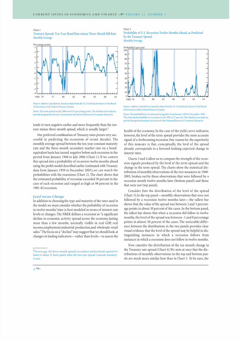
tends to turn negative earlier and more frequently than the ten-year minus three-month spread, which is usually larger.6

Our preferred combination of Treasury rates proves very suc-cessful in predicting the recessions of recent decades. Themonthly average spread between the ten-year constant maturityrate and the three-month secondary market rate on a bond-equivalent basis has turned negative before each recession in theperiod from January 1968 to July 2006 (Chart 1). If we convert

this spread into a probability of recession twelve months aheadusing the probit model described earlier (estimated with Treasurydata from January 1959 to December 2005), we can match theprobabilities with the recessions (Chart 2). The chart shows thatthe estimated probability of recession exceeded 30 percent in thecase of each recession and ranged as high as 98 percent in the1981-82 recession.

Level versus Change

In addition to choosing the type and maturity of the rates used inthe model, we must consider whether the probability of recessionin twelve months’ time is best modeled in terms of interest rate

levels or changes. The NBER defines a recession as “a significantdecline in economic activity spread across the economy, lasting

more than a few months, normally visible in real GDP, realincome,employment,industrial production,and wholesale-retailsales.”The focus on a “decline”may suggest that we should look atchanges in leading indicators—rather than levels—to assess the

health of the economy. In the case of the yield curve indicator,

however, the level of the term spread provides the most accuratesignal of a forthcoming recession.One reason for the superiorityof this measure is that, conceptually, the level of the spreadalready corresponds to a forward-looking expected change ininterest rates.

Charts 3 and 4 allow us to compare the strength of the reces-

sion signals produced by the level of the term spread and thechange in the term spread. The charts show the statistical dis-tribution of monthly observations of the two measures in 1968-2005, broken out by those observations that were followed by arecession month twelve months later (bottom panel) and thosethat were not (top panel).

Consider first the distribution of the level of the spread(Chart 3).In the top panel—monthly observations that were notfollowed by a recession twelve months later—the tallest barshows that the value of the spread was between 2 and 3 percent-age points in about 30 percent of the cases. In the bottom panel,

the tallest bar shows that when a recession did follow in twelve

months, the level of the spread was between -1 and 0 percentagepoints in almost 50 percent of the cases. The noticeable differ-ence between the distributions in the two panels provides clearvisual evidence that the level of the spread may be helpful in dis-tinguishing instances in which a recession follows frominstances in which a recession does not follow in twelve months.

Now consider the distribution of the six-month change inthe Treasury rate spread (Chart 4).We note at once that the dis-tributions of monthly observations in the top and bottom pan-els are much more similar here than in Chart 3. To be sure, the

4

Source: Authors’ calculations, based on data from the H.15 statistical release of the Board

of Governors of the Federal Reserve System.Notes: The term spread in July 2006 was 0.01 percentage point. The shaded areas indicate

periods designated national recessions by the National Bureau of Economic Research.

Chart 1

Treasury Spread: Ten-Year Bond Rate minus Three-Month Bill RateMonthly Average

Percentage points

-4

-3

-2

-1

0

1

2

3

4

5

05009590858075701968

Source: Authors’ calculations, based on data from the H.15 statistical release of the Boardof Governors of the Federal Reserve System.

Notes: The probabilities are estimated using data f rom January 1959 to December 2005.The estimated probability of recession in July 2007 is 27 percent. The shaded areas indicate

periods designated national recessions by the National Bureau of Economic Research.

Chart 2

Probability of U.S. Recession Twelve Months Ahead, as Predictedby the Treasury SpreadMonthly Average

Probability ( percent)

0

10

20

30

40

50

60

70

80

90

05009590858075701968

100

6On average, the three-month spread (secondary market bond-equivalentbasis) is about 21 basis points when the two-year spread (constant maturity)is zero.




observations in the top panel are skewed to the right while obser-vations in the bottom panel are slightly skewed toward morenegative levels—a qualitative pattern similar to that found inChart 3. Nevertheless, it is clear that the ability to discriminatebetween recessionary and nonrecessionary instances is muchmore limited with changes than with levels.

A simple example provides further evidence of the weaknessof the change in the spread as an indicator. In May 1990, theaverage spread was 76 basis points. In June, it decreased by27 basis points to 49. This decline resulted in an increase of 7.1 percentage points in the implied probability of recession. By

contrast, when the average spread decreased 27 basis pointsbetween January and February of 1993, from 3.54 to 3.27 per-centage points, the implied probability of recession declined byless than 0.1 percentage point. These contrasting episodes sug-gest that the change in the spread may provide an arbitrary sig-nal, one that varies greatly with the steepness of the yield curve:in general, the steeper the yield curve, the smaller the impact of

a given change on the implied probability of recession. Hence,the change in the spread by itself is not very informative.

Interpreting the SignalHaving established that tracking the level of the ten-year tothree-month Treasury spread is useful in predicting recessions,we now consider how best to interpret the signal sent by thismeasure. The lower panel of Chart 3 suggests that, of the obser-vations followed by a recession twelve months later, 69 percent(the sum of the bars to the left of zero) are negative. Thus, one

could look to an inversion of the yield curve as a signal.However, there still may be some question regarding thestrength of the signal. Does the signal have to be persistent?

How strong must it be? Does it matter if the inversion is drivenby changes in the long end or short end of the yield curve? Thenext two sections reveal that persistent negative signals, no

matter how slight, are reliable predictors and that the modeldoes not depend on particular movements at the long end of the curve.

Persistence and Strength

Market chatter tends to pick up at the slightest sign of a yieldcurve inversion, regardless of size or duration, even intraday.However, inversions in daily or intraday data often prove tobe false signals. Inversions observed over longer periods—ata monthly or quarterly average frequency—provide morereliable signals.

Consider, for example, that all six NBER recessions since

1968 have been preceded by at least three negative monthlyaverage observations in the twelve months before the start of the recession (see table). Moreover, when inversion on a

monthly average basis is used as an indicator, there have beenno false signals over this period. By contrast, negative spreadsoccurred on 100 days between January 1, 1968, and December 31,2005, in months that did not turn out to have negative averagemonthly spreads.

Although inversion has been a dependable recession signal inrecent decades, the precise level of the negative spread has varied

Chart 3

Frequency Distribution of Level of Spread

Percentage of observations

0

10

20

30

40

50

0

10

20

30

40

50

6543

210-1-2-3

-4-5-6-7

One year before nonrecession month

One year before recession month

Level of spread (percentage points)


Note: The frequency distribution is estimated u sing data from 1968 to 2005.

Chart 4

Frequency Distribution of Six-Month Change in Spread

Percentage of observations

0

10

20

30

40

50

0

10

20

30

40

50

6543

210-1-2-3

-4-5-6-7

One year before nonrecession month

One year before recession month

Six-month change in spread (percentage points)


Note: The frequency distribution is estimated using data from 1968 to 2005.




with each recession.7 The table shows the lowest monthly averagelevel of the spread between ten-year and three-month Treasury

rates in the twelve months preceding each recession since 1968.In this case, we look at the lowest level of the spread because itprovides the strongest signal. Two clear features emerge from thetable: the spread has always been negative (the yield curve hasinverted at these maturities), and the level at which the spreadhas bottomed out differs considerably across recessions—from alow value of -3.51 to a slightly negative value of -0.08. We note,however, that while we focus here on predicting the occurrenceand not the severity of recessions, there is evidence that more

pronounced inversions—as in the early 1980s—have generallybeen associated with deeper subsequent recessions.8

In sum, it seems most appropriate to look at the spread as a

recession indicator on at least a monthly average basis. If thespread is calculated from ten-year and three-month bond-equivalent rates, an inversion—even a slight one—is a simpleand historically reliable benchmark.

Short-End versus Long-End Changes

Just as the strength of the inversion has no bearing on the abil-ity of the model to predict a recession, so it is also immaterialhow the inversion is influenced by changes at the long end of the yield curve. The performance of the yield spread as an indi-cator does not seem to depend on the particular behavior of thelong-term rate in isolation.

Monetary policy most directly influences the short end of theyield curve, although it may affect the level of long-term ratesthrough expectations.An increase in short-term policy rates fre-quently results in higher longer term rates as well, though the riseat the long end is typically smaller. At times, the long rates move

in the opposite direction. Either case, if persistent, may result inan inversion of the yield curve. On occasion, long-term ratesdecline without a clear simultaneous movement in short-term

rates,a pattern that may also result in an inversion.

Chart 5 displays the level of the three-month Treasury rate(blue line) and the change in this rate over the eighteen monthsleading to peak recession signals since 1968 (green bars). Thetiming of the peak signals corresponds to the low monthly aver-age spread levels reported in the table. We observe that the greenbars in the chart are all positive, indicating that a rise in thethree-month rate preceded each recession during this period. Inthat sense,we could think of every yield curve inversion as result-ing at least partly from a rise at the short end.

Chart 6 performs the same analysis for the ten-year Treasury

rate, and we see that its behavior is not as consistent as that of the short rate. Prior to the first four recessions, the long end of the yield curve rose as the y ield spread signal was unfolding.

Prior to the last two recessions, the long rate actually declined,contributing more directly to the yield curve inversion.

The evidence from Chart 6 suggests that the performance of the yield curve as an indicator does not depend on the movements

of the long-term rate. The inversion in 1981 was the most pro-nounced in this period. Contrary to what one might expect, thelong rate did not decline but instead experienced its largest rise in

6

7In the 1950s and early 1960s, there were cases in which the yield curve wasalmost flat, but did not invert in anticipation of recessions. Since 1968,however,the signal from the spread between the Treasury ten-year and three-monthrates has always been negative before recessions, and very low positive spreadshave not been followed by recessions. See Arturo Estrella,“The Yield Curve as aLeading Indicator: Frequently Asked Questions,” <http://www.newyorkfed.org/research/capital_markets/ycfaq.html>.

8See, for example,Estrella and Hardouvelis (1991).

Magnitude of Term Spread Signals Twelve Months beforeEach Recession since 1968

Number ofMonths with Minimum LevelNBER Recession Negative Monthly Spreads ofSpread

January 1970 – November 1970 10 -0.51

December 1973 – March 1975 6 -1.59February 1980 – July 1980 12 -2.20

August 1981 – November 1982 10 -3.51

August 1990 – March 1991a 3 -0.08

April 2001 – November 2001 7 -0.70

Source:Authors’calculations, based on data from the H.15 statistical release of theBoard of Governors of the Federal Reserve System.

aNote that the value of the term spread was -0.16 in June 1989, fourteen monthsbefore the recession.


Notes: The green bars represent the change in the three-month Treasury bill rate over theeighteen months leading to peak recession signals since 1968. The shaded areas indicateperiods designated national recessions by the National Bureau of Economic Research.

Chart 5

Short-Term Rate around Peak Recession SignalsLevel of Rate and Eighteen-Month Change in Rate at Peak Signal from Spread

Three-month Treasury bill rate (percentage points)

0

5

10

15

20

05009590858075701968



anticipation of the recession. Conversely, the last two inversionswere accompanied by declines in the long rate but were not par-ticularly large in magnitude.

ConclusionsOur analysis suggests a number of practical guidelines for theuse of the yield curve to predict recessions in real time:

●

Defining recessions as the periods between NBER peaksand troughs—counting the troughs but not the peaks—produces clear results.

● Treasury rates are most likely to produce accurate forecasts.

● The best maturity combination may be three months andten years.Other choices lead to results that are highly cor-related with our own, but whatever combination isselected should be used consistently in both analysis andprediction.

● The three-month rate is best represented by the second-ary market rate, expressed on a bond-equivalent basis tomatch the ten-year rate.

● The ten-year constant maturity rate produces good results.

● Levels of the spread are more informative than changes.

As for why the yield curve is such a good predictor of reces-

sions, we have reviewed a number of possible reasons, each of which may play an important role at different times. The consis-tency with which these explanations relate a yield curve flatteningto slower real activity provides some assurance that the indicator isvalid. Nevertheless, in the end, we must remind ourselves thatthe evidence of the yield curve’s predictive power is statisticaland that, however accurate past signals have been,it is impossibleto guarantee future results.

References

Eijffinger, Sylvester, Eric Schaling, and Willem Verhagen. 2000. “The TermStructure of Interest Rates and Inflation Forecast Targeting.” Centre forEconomic Policy Research Discussion Paper no.2375.

Estrella,Arturo. 2005.“Why Does the Yield Curve Predict Output and Inflation?”

Economic Journal 115,no.505 ( July): 722-44.

Estrella,Arturo, and Gikas Hardouvelis. 1991.“The Term Structure as a Predictorof Real Economic Activity.” Journal of Finance 46,no. 2 (June): 555-76.

Estrella,Arturo, and Frederic S.Mishkin. 1996.“The Yield Curve as a Predictor of U.S. Recessions.” Federal Reserve Bank of New York Current Issues in

Economics and Finance 2,no.7 (June).

Estrella, Arturo,Anthony P. Rodrigues, and Sebastian Schich.2003. “How StableIs the Predictive Power of the Yield Curve? Evidence from Germany and theUnited States.” Review of Economics and Statistics 85,no. 3 (August): 629-44.

Hardouvelis, Gikas, and Dimitrios Malliaropulos. 2004.“The Yield Spread as aSymmetric Predictor of Output and Inflation.” Centre for Economic PolicyResearch Discussion Paper no.4314.

Harvey, Campbell R. 1988.“The Real Term Structure and Consumption Growth.” Journal of Financial Economics 22,no. 2 (December): 305-33.

Rendu de Lint,Christel, and David Stolin. 2003.“T he Predictive Power of theYield Curve: A Theoretical Assessment.” Journal of Monetary Economics 50,no.7 (October): 1603-22.

Wright, Jonathan H. 2006.“The Yield Curve and Predicting Recessions.” Board of Governors of the Federal Reserve System, Finance and EconomicsDiscussion Series, no. 2006-07,February.


The views expressed in this article are those of the authors and do not necessarily reflect the

position of the Federal Reserve Bank of New York or the Federal Reserve System.

About the Authors

Arturo Estrella is a senior vice president in the Capital Markets Function of the Research and Statistics Group; Mary R. Trubin, formerly

an economist in the Capital Markets Function, is entering the Ph.D. program in economics at Northwestern University.

Current Issues in Economics and Finance is published by the Research and Statistics Group of the Federal Reserve Bank of New York.

Leonardo Bartolini and Charles Steindel are the editors.

Source: Authors’ calculations, based on data from the H.15 statistical release of the Board

of Governors of the Federal Reserve System.

Notes: The green bars represent the change in the ten-year Treasury bond rate over theeighteen months leading to peak recession signals since 1968. The shaded areas indicateperiods designated national recessions by the National Bureau of Economic Research.

Chart 6

Long-Term Rate around Peak Recession SignalsLevel of Rate and Eighteen-Month Change in Rate at Peak Signal from Spread

Ten-year Treasury bond rate (percentage points)

-2

0

2

4

6

8

10

12

14

16

05009590858075701968



C urrent I ssuesF E D E R A L R E S E R V E B A N K O F N E W Y O R K

C urrent I ssuesIN ECONOMICS AND FINANCE

3 L I B E R T Y S T R E E T N E W Y O R K , N Y 1 0 0 4 5

T h e Y i e l d C u r v e a s a L e a d i n g I n d i c a t o r : S o m e P r a c t i c a l I s s u e s A r t u r o E s t r e l l a a n d M a r y R . T r u b i n

S i n c e t h e 1 9 8 0 s , e c o n o m i s t s h a v e a r g u e d t h a t t h e s l o p e o f t h e y i e l d c u r v e — t h e s p r e a d b e t w e e n l o n g - a n d s h o r t - t e r m i n t e r e s t r a t e s — i s a g o o d p r e d i c t o r o f f u t u r e e c o n o m i c a c t i v i t y . W h i l e m u c h o f t h e e x i s t i n g r e s e a r c h h a s d o c u m e n t e d h o w c o n s i s t e n t l y m o v e m e n t s i n t h e c u r v e h a v e s i g n a l e d

p a s t r e c e s s i o n s , c o n s i d e r a b l y l e s s a t t e n t i o n h a s b e e n p a i d t o t h e u s e o f t h e y i e l d c u r v e a s a f o r e c a s t i n g t o o l i n r e a l t i m e . T h i s a n a l y s i s s e e k s t o f i l l t h a t g a p b y o f f e r i n g p r a c t i c a l g u i d e l i n e s o n h o w b e s t t o c o n s t r u c t t h e y i e l d c u r v e i n d i c a t o r a n d t o i n t e r p r e t t h e m e a s u r e i n r e a l t i m e .

C u r r e n t I s s u e s C u r r e n t I s s u e s I N E C O N O M I C S A N D F I N A N C E

w w w . n e w y o r k f e d . o r g / r e s e a r c h / c u r r e n t _ i s s u e s

V o l u m e 1 2 , N u m b e r 5 J u l y / A u g u s t 2 0 0 6

F E D E R A L R E S E R V E B A N K O F N E W Y O R K w w w . n e w y o r k f e d . o r g / r e s e a r c h / c u r r e n t _ i s s u e s

Documents

The Yield Curve as a Leading Indicator