The Yield Curve as a Leading Indicator: Frequently Asked Questions

Arturo Estrella October 2005 

broad literature originating in the late 1980s documents the empirical regularity that the slope of the yield curve is a reliable predictor of future real economic activity. Today, there exists a substantial body of evidence from 

which various useful stylized facts have emerged. This catalogue of some of the salient findings takes the form of answers to frequently asked questions. An extensive bibliography is also included. 

A  Click on a question from the following list to go to the page containing the answer.  Q. What does the evidence say, in short?Q. How and when were the relationships first identified?Q. How long have these relationships existed, and do they still hold? Q. Are  formal models needed  to extract  the  information content  in  the yield curve, or 

are there also rules of thumb? Q. What statistical models have been formulated? Q. Which interest rates to use: Treasuries, fed funds, Eurodollar, swap, corporate? Q. What maturity combinations work best? Q. Is it the level or the change in the spread that matters? Q. Does it matter if changes are driven by the short or the long end? Q. Is an inversion required for a signal? Q. Does the signal have to be persistent? Q. Is the evidence robust over time? Q. How do binary models  that predict  recessions  compare with models  that  forecast 

continuous dependent variables (e.g., real GDP, industrial production growth)?  Q. How does the yield curve compare with other indicators?  Q. How does the yield curve perform out of sample, and can it be supplemented with 

other indicators? Q. How are predictions related to monetary policy? Q. How are predictions related to market expectations of the economy? Q. Is there causality from economic activity to the yield curve? Q. Should we expect the predictive power of the term spread for real activity to persist?  Note: Views expressed are the author’s and do not necessarily represent those of the Federal Reserve Bank of New York or the Federal Reserve System. 

1

Questions & Answers  Q. What does the evidence say, in short? A. The difference  between  long‐term  and  short‐term  interest  rates  (“the  slope  of  the yield  curve” or  “the  term  spread”) has borne  a  consistent negative  relationship with subsequent real economic activity in the United States, with a lead time of about four to six quarters. The measures of  the yield curve most  frequently employed are based on differences between  interest  rates on Treasury  securities of  contrasting maturities,  for instance,  ten  years  minus  three  months.  The  measures  of  real  activity  for  which predictive  power  has  been  found  include  GNP  and  GDP  growth,  growth  in consumption, investment and industrial production, and economic recessions as dated by  the National Bureau of Economic Research  (NBER). The  specific accuracy of  these predictions depends on the particular measures employed, as well as on the estimation and prediction periods. However,  the results are generally statistically significant and compare  favorably with other variables employed as  leading  indicators. For  instance, models that predict real GDP growth or recessions tend to explain 30 percent or more of the variation  in  the measure of  real activity. See Estrella and Hardouvelis  (1991). The yield  curve  has  predicted  essentially  every U.S.  recession  since  1950 with  only  one “false” signal, which preceded the credit crunch and slowdown in production in 1967. There is also evidence that the predictive relationships exist in other countries, notably Germany,  Canada,  and  the  United  Kingdom.  See  Estrella  and Mishkin  (1997)  and Bernard and Gerlach (1998). [See also Box 1] Back to questions. Q. How and when were the relationships first identified? A. Analysis of  the behavior of  interest  rates of different maturities over  the business cycle goes back at  least  to Mitchell  (1913). However, Kessel  (1965) may have been  the first  to  make  specific  reference,  verbal  if  not  quantitative,  to  the  behavior  of  term spreads. He pointed out that various spreads between  long‐ and short‐term rates tend to be  low at the start of recessions – the business cycle peak – and high as expansions get under way after a cyclical trough. Butler (1978) made a connection between the yield curve as a predictor of short‐term interest rates and the implications of declining short‐term  rates  for  contemporaneous  economic  activity,  foreshadowing  some  of  the  later logic. He correctly predicted  that  there would be no  recession  in 1979,  though a year later  the  situation  would  have  been  quite  different.  The  late  1980s  saw  a  spurt  in research on  the yield curve as a  leading  indicator. Laurent  (1988, 1989) used  the  term spread  to  predict  GNP  growth.  Harvey  (1988)  developed  a  theoretical  relationship between the real term spread and subsequent real consumption growth, and presented some confirming empirical evidence. Furlong  (1989) noted some predictive power  for recessions,  but  expressed  skepticism  about  the  yield  curve’s  reliability  as  a  leading 

2

indicator at  that  time. Estrella and Hardouvelis  (1989, 1990, 1991) showed empirically that  the yield  curve may be used  to predict  real growth  in  consumption,  investment, and  aggregate  GNP,  as  well  as  NBER‐dated  recessions.  Stock  and  Watson  (1989) developed  a  sophisticated model  of  coincident  and  leading  indicators, with  the  term spread forming part of the latter. Chen (1991) looked at the predictive relationship from the point of view of financial market investors. [See also Box 2] Back to questions. Q. How long have these relationships existed, and do they still hold?  A. Kessel (1965) presents graphical evidence that shows that the term spread tends to be negative  at  cyclical  peaks,  using  data  that  go  back  as  far  as  1858.  He  finds  some evidence of the leading indicator properties of the spread in time periods from 1914 to 1933  and  from  1954  to  1961.  Bordo  and  Haubrich  (2004)  provide  regression‐based statistical  evidence  using U.S.  data  from  1875  to  1997  and  Baltzer  and  Kling  (2005) perform a similar exercise with German data from 1870 to 2003. Both papers conclude that predictability varies over  time and  that  it seems  to be related  to monetary policy credibility. Most other  studies use data  since  the 1950s. The most  recent data suggest that some of the statistical models from which forecasts based on the term structure are constructed have undergone structural changes, particularly with regard  to parameter values. The predictive power may still be  there, but  the values of  the parameters  that record the sensitivity to movements in the term spread may be somewhat changed from earlier periods. However, the simple rule of thumb that the difference between ten‐year and three‐month Treasury rates turns negative in advance of recessions is still reliable, with negative values observed before both the 1990‐1991 and 2001 recessions. [See also Box 4] Back to questions. Q. Are  formal models needed  to extract  the  information content  in  the yield curve, or are there also rules of thumb?  A. Much of the research on this topic has been based on formal statistical models, such as linear regressions and non‐linear statistical equations. These models are useful in that they provide quantitative guidelines about the sensitivity of output growth to changes in  the  term  spread and about  the precise  lead‐lag  relationships exhibited by  the data series,  as  well  as  recession  probabilities.  Nevertheless,  simple  rules  of  thumb  are available,  such  as  the  fact  that  yield  curve  inversions  (negative  term  spreads)  are followed by recessions. Estrella and Mishkin (1996b) and Estrella (2005b) show that this approach  may  be  made  a  bit  more  precise,  though  still  simple,  by  presenting  the relationship in tabular or graphical form. [See also Box 3] Back to questions. Q. What statistical models have been formulated?  A. Much of  the analysis  in  the  literature has  focused on “continuous variables,” data series whose values can in principle be any real numbers. Examples of these series are 

3

growth  rates  in GNP, GDP,  industrial production,  consumption,  and  investment. To predict  these  series,  analysts  have  generally  relied  on  relatively  standard  regression equations, taking care to deal with some important statistical issues. The most common issue results from the presence of overlapping observations in many of the applications. For example, suppose  that we are  interested  in  forecasting GDP growth over  the next year  using  quarterly  data.  Then,  two  consecutive  observations  of  the  variable  being forecasted  correspond  to  time periods  that have  three quarters  in  common. Standard measures of statistical significance are in general inconsistent, and must be adjusted by using, for instance, the generalized method of moments estimators of Hansen (1982) or Newey and West  (1987). When  the objective  is  to predict recessions,  the methodology used  is  typically  a  probit  or  logit  equation,  in  which  the  forecasted  variable  only assumes the values one and zero (either the economy is in a recession or it is not). Note, however,  that  special  techniques  are  also  required  in  these  models  if  the  forecast horizon produces overlapping observations. See Estrella and Rodrigues (1998). Back to questions. Q. Which interest rates to use: Treasuries, fed funds, Eurodollar, swap, corporate?  A. Research on  the United States business cycle has relied mostly on  interest rates  for U.S.  Treasury  securities.  One  reason  is  convenience:  data  for  many  maturities  are available  continuously  from  the  1950s  to  the present  in  a  consistent  format. Another reason  is  that  the  pricing  of  these  securities  is  not  subject  to  significant  credit  risk premiums  that,  at  least  in  principle, may  change with maturity  and  over  time.  For similar reasons, studies of other countries tend to use data on national government debt securities. Rates on coupon bonds and notes are most easily accessible, but researchers in  many  countries  have  also  produced  zero‐coupon  rates,  which  may  be  directly matched with  the  timing of  the  forecasts. Some analysts have also used, as short‐term rates, the U.S. federal funds rate and rates closely controlled by central banks  in other countries. These are useful for some purposes, but the control exercised by the central bank  implies  that  these  rates  are  not  fully  reflective  of  the  expectations  of  financial market participants. The  spread between  ten‐year Treasuries and  fed  funds  is a very accurate predictor of U.S. recessions during some time periods, but less so in others. At certain times, concerns have been voiced that special factors, such as the federal budget surpluses of 1999‐2000, might affect  the supply or demand of Treasury securities and distort  the signals  incorporated  in  their prices. Attempts have been made  to use other interest  rates  for which  a  yield  curve may  be  constructed,  like  Eurodollar,  swap  or corporate  rates.  An  important  drawback  to  the  use  of  such  data,  however,  is  their limited  availability with  regard  to  the  length  of historical  time  series,  the number of points along the yield curve, or both. Back to questions. 

4

Q. What maturity combinations work best?  A. When the yield curve is used to predict inflation (e.g., as in Mishkin (1990a, 1990b), interest  rate maturities are matched precisely with  the  forecast horizons  for  inflation. For instance, to predict the difference between inflation expected in the next five years and  inflation expected  in  the next year,  the difference between  five‐year and one‐year Treasury yields  is used. When forecasting real activity,  in contrast, the best results are obtained  empirically  by  taking  the  difference  between  two  Treasury  yields  whose maturities are  far apart. At  the  long end,  the clear choice seems  to be a  ten‐year  rate, which  is  the  longest maturity available  in most countries on a consistent basis over a long sample period. At the short end, there is a wider variety of choices. An overnight rate,  such  as  the  fed  funds  rate,  is  close  to  the  extreme  of  the maturity  spectrum. However,  its  usefulness  as  an  indicator  of market  expectations  is  confounded  by  its fairly direct control by the Federal Reserve. A common choice currently is the two‐year Treasury  rate,  perhaps  because  of  the  liquidity  of  the  associated  instruments. Background research in connection with Estrella and Mishkin (1998) suggested that the three‐month Treasury rate, when used  in combination with  the  ten‐year Treasury rate to  predict  U.S.  recessions,  provides  a  reasonable  combination  of  accuracy  and robustness over long time periods. In the end, most term spreads are highly correlated and provide similar information about the real economy, so the particular choices with regard  to maturity  amount mainly  to  fine  tuning  and  not  to  reversal  of  results. The caveat  is  that a benchmark  that works  for one  spread may not work  for another. For instance, the ten‐year minus two‐year spread may invert earlier than the ten‐year minus three‐month spread, which tends to be larger. Back to questions. Q. Is it the level or the change in the spread that matters?  A.  With  many  leading  economic  indicators,  either  individual  variables  or  indices, analysts focus on the change or growth rate in the variable as a forecaster of future real economic conditions. In contrast, it is the level of the term spread – not the change – that helps forecast both recessions and changes in real economic activity. For recessions, it is clearly the level that matters. In a probit model of the probability of recession, a given change in the spread can have a very different impact, depending on the initial level of the  spread. When  the  curve  is very  steep,  say  the  spread  is above 300 basis points, a change  of  50  basis  points  in  the  spread  hardly  changes  the  probability  of  recession. However, if the spread starts out at 50 basis points, a decrease of that magnitude may raise the implied probability by 10 percentage points or more. Theoretical explanations of these empirical results are not easily formulated. A suggestive heuristic argument is that  the  term spread, being a difference between  interest  rates of different maturities, incorporates an  element of  expected  changes  in  rates and  is  thus  indicative of  future changes in real activity. In 1996, the Conference Board added the yield curve spread to its  index  of  leading  indicators,  focusing  on  monthly  changes  in  the  spread.  Note, 

5

however,  that  it announced  in  June 2005  that  it would adjust  its procedures  so as  to focus  on  the  level  of  the  spread  and  not  on  the  change.  [See  also  Box  3]  Back  to questions. Q. Does it matter if changes are driven by the short or the long end?  A. The best forecast of future real activity  is provided by the  level of the term spread, not the change in the spread, nor even the source of the change in the spread. Thus, if a low or negative value of the spread is reached via an increase in the short‐term rate or a decrease  in  the  long‐term  rate,  it  is only  the  low  level  that matters.  In  the six months preceding the trough of each yield curve inversion in the United States since 1960, we see a decline  in  the  ten‐year Treasury rate  in  two of seven cases  (before  the 1990‐1991 and 2001 recessions) and an  increase  in the other cases. The direction of the change  in the ten‐year rate at the time of the signal does not appear to be indicative of the strength or  duration  of  the  subsequent  recession.  It  is  clear,  however,  that  each  recessionary episode is preceded (with varying lead times) by a substantial increase in the short‐term rate. Back to questions. Q. Is an inversion required for a signal?  A. Although  economic  theory  suggests  that  the yield  curve  should help  forecast  real output,  no  theory  establishes  a  clear  connection  specifically  between  yield  curve inversions and recessions. However, since 1960, a yield curve inversion (as measured by the difference between  ten‐year  and  three‐month Treasury  rates) has preceded  every recession on record. In fact, in terms of monthly averages, the ten‐year rate was at least 12  basis  points  below  the  three‐month  rate  before  every  recession  in  that  period.  In contrast,  very  low  positive  levels  of  the  spread  have  been  observed  without  a subsequent  recession. Specifically,  there were  two episodes  in  the 1990s  in which  the term spread attained very low positive levels (42 and 12 basis points respectively), but did not  invert.  In both of  those cases, economic activity continued unabated after  the troughs or low points for the spread. Thus, using inversion as a benchmark, there were no  “false  positives”  during  the  period. While  inversions  and  recessions may  not  be inevitably connected by  theory,  they correspond  to extreme values of  the  term spread and output growth, respectively, which are in fact theoretically linked. [See also Box 5] Back to questions. Q. Does the signal have to be persistent?  A. Daily or even intraday changes in the term spread can be substantial. For example, for  the spread between  ten‐year and 3‐month  rates, one‐day changes of over 25 basis points occur about 2½ percent of the time. In some cases, these changes may be driven by market expectations of economic fundamentals and consequently may be persistent. In many  instances,  though,  high‐frequency  changes  in  the  spread may  result  from 

6

temporary demand or supply imbalances in the markets for Treasury securities, which may be quickly reversed and thus may not be truly reflective of changes in expectations about real economic conditions. One way to distinguish between perceived changes in fundamentals  and  temporary market  phenomena  is  to  trace  the  persistence  of  yield curve  signals. A  signal  that  lasts  only  one  day may  be  dismissed,  but  a  signal  that persists  for  a  month  or  more  should  be  looked  at  carefully.  Statistically,  these distinctions may be captured by using data averaged over one month or more, which is quite  common  in  the  literature,  or  by  including  lagged  effects  in  the model,  as  in Chauvet and Potter (2005). Back to questions. Q. Is the evidence robust over time?  A. An informal way to assess the robustness of yield curve forecasts of real activity is to examine  visually  the  ex  post  accuracy  of  the  results.  In  some  cases,  as  with  the regularity that yield curve inversions precede recessions, the evidence is immediate and quite consistent, as in the United States since 1960. The only apparent miss was in 1967, when  the economy experienced a “credit crunch”  that  the NBER did not classify as a recession,  despite  a marked  decline  in  industrial  production.  In  other  cases,  such  as with forecasts of real GDP growth, it is not altogether obvious whether the forecasting performance  is  consistent  in different  subperiods. Thus,  it  is helpful  to  apply  formal statistical tests of model stability to the forecasting equations. Stock and Watson (2003) find instability in a large proportion of the models that are frequently used to forecast output growth. Their results stress the need to look for changes in parameter values that may  result,  for  instance,  from changes  in monetary policy  regime. Estrella, Rodrigues and Schich (2003) find modest evidence of instability in models used to forecast growth in  industrial production, which suggests a similar caveat. However,  the  latter  find no evidence of instability in models used to forecast recessions in Germany and the United States, suggesting that models with qualitative dependent variables may be more robust to changes in policy or other economic conditions. Back to questions. Q. How do binary models  that predict  recessions  compare with models  that  forecast continuous dependent variables (e.g., real GDP or industrial production growth)?  A.  These  two  types  of models may  be  compared  in  two  dimensions:  accuracy  and robustness. There  is evidence  that  the most accurate binary models perform about as well  as  the most  accurate  continuous models. For  example, Estrella  and Hardouvelis (1991) and Estrella and Mishkin (1997) find that the R‐squared in models of cumulative GNP  growth  is  similar  in magnitude  to  the  pseudo  R‐squared  in  probit models  of recession. The  sample period may  influence  the  results  somewhat, particularly  in  the case of  the  continuous models. Stock  and Watson  (2003)  find  substantial  evidence of instability over  time  in various models of output growth, and Estrella, Rodrigues and Schich (2003) find some instability in models of industrial production growth. However, 

7

the  latter paper  suggests  that binary models of  recessions are quite  robust over  time, both in Germany and in the United States. Back to questions. Q. How does the yield curve compare with other indicators?  A.  In general,  the yield  curve  tends  to perform quite well  in  comparisons with other leading indicators, including the traditional leading indexes and their components, and other  variables with  potential  predictive  power.  Indicators  such  as  stock  prices  and interest  rates may have  similar performance  to  the yield  curve at  some horizons, but none seem to dominate the yield curve as a predictor. For instance, Dueker (1997) and Dotsey (1998) compare the yield curve with a few other variables as a leading indicator of  recessions, and  find generally  supportive  statistical evidence. Estrella and Mishkin (1998) compare  the  term structure as a predictor of recessions with a  large number of alternative  indicators,  and  find  that  it  is  among  the  best  in  tests  of  statistical significance,  particularly  at  horizons  of  about  one  year.  Stock  and  Watson  (2003) examine a large number of competing indicators in forecasts of output growth and find that all of them fall short of ideal properties, but that within these limitations the term structure “comes closest” to achieving those goals. Back to questions. Q. How does the yield curve perform out of sample, and can it be supplemented with other indicators?  A. The yield curve performs quite well in out of sample tests of predictive accuracy, and it  is not  clear  that,  in general,  supplementary  information  can  improve  its predictive performance. Estrella and Mishkin  (1998)  find  that, at predictive horizons beyond one quarter, there  is no match for the term structure as a predictor of recessions. Not only do  a  large number  of  other  indicators  fall  short,  but predictions deteriorate  as  those other  indicators  are  added  to  the  term  spread  in out of  sample  forecasting  exercises. Stock and Watson (2003) similarly examine a large number of competing indicators, but focus  on  forecasts  of  output  growth  rather  than  recessions.  They  find  that  the  term spread works best, but  that  it  exhibits  some  instability. The nature  of  this  instability seems  sufficiently  idiosyncratic  that  combining  the  term  spread  with  some  other indicators may improve performance in their equations. Back to questions. Q. How are predictions related to monetary policy?  A. Although  there  are  different  views  of  the  instruments  and  channels  of monetary policy, a tightening of monetary policy usually means a rise in short‐term interest rates, typically  intended  in  the  end  to  lead  to  a  reduction  in  inflationary  pressures. When those pressures subside, it is expected that a policy easing will follow. Expected future short‐term rates are important determinants of current long‐term rates. Thus, long rates tend  to  respond  to  a monetary  tightening  by  increasing,  though  given  that  a  policy reversal  is expected, they tend not to  increase by as much as short‐term rates. Thus, a 

8

simple explanation of the predictive power of the yield curve for future output growth is  that  a monetary  tightening  both  slows  down  the  economy  and  flattens  (or  even inverts)  the yield curve. Monetary policy  is  therefore an  important determinant of  the predictive power of the yield curve. However, given that private‐sector expectations are incorporated  in  interest  rates,  and  given  that  those  expectations  are  based  on  some concept of the structure of  the economy, monetary policy  is not  likely  to be  the single determinant  of  the  predictive  power.  Formal  models  with  these  properties  are presented  in Eijffinger, Schaling and Verhagen  (2000), Hardouvelis and Malliaropulos (2004), and Estrella (2005a). Back to questions. Q. How are predictions related to market expectations of the economy?  A. One  of  the most  pervasive  theories  of  the  determinants  of  the  yield  curve  is  the expectations  hypothesis,  which  posits  that  long‐term  interest  rates  are  averages  of expected  future  short‐term  rates.  In  the  “pure”  version  of  the  hypothesis,  this  is  the whole  story.  That  version  has  been  repeatedly  rejected  in  econometric  tests  [see Campbell (1995)], so it is likely that there are other important determinants as well, such as  risk or  liquidity premiums. Nevertheless,  it  is difficult  to dispute  that  interest  rate expectations play an  important  role, and  that  those expectations are  related  to  future real demand for credit and to future inflation. A rise in short‐term interest rates induced by monetary  policy may  lead  to  a  future  slowdown  in  real  economic  activity  and demand for credit, putting downward pressure on future real interest rates. At the same time,  slowing  activity  may  result  in  lower  expected  inflation.  By  the  expectations hypothesis,  these  expected  declines  in  future  short‐term  rates would  tend  to  reduce current  long‐term  rates and  flatten  the yield curve. Clearly,  this scenario  is consistent with the observed correlation between the yield curve and recessions. A formal model with these properties is presented in Estrella (2005a), and alternative specifications are considered in Eijffinger, Schaling and Verhagen (2000), Rendu de Lint and Stolin (2003), Malliaropulos (2003) and Hardouvelis and Malliaropulos (2004). Back to questions. Q. Is there causality from economic activity to the yield curve?  A. Most of the literature in this field deals with the yield curve as a predictor of future activity,  but  in  principle  there  could  be  influences  in  the  opposite  direction,  from economic  activity  to  the  yield  curve.  In  a  dynamic  theoretical model  with  rational expectations,  such  as  Estrella  (2005a),  both  directions  play  a  role.  The  term  spread contains expectations of  future activity, and  it  is affected by current monetary policy, which  is  influenced  in  turn  by  current  economic  activity.  Empirically,  Estrella  and Hardouvelis (1990) use U.S. data to examine the effect of monetary policy on the yield curve,  and  Estrella  and  Mishkin  (1997)  perform  a  similar  analysis  for  a  panel  of European economies. Evans and Marshall (2001) find consistent evidence that monetary policy shocks affect the nominal yield curve. In the context of a vector autoregression, 

9

Diebold, Rudebusch  and Aruoba  (2004)  find  that  the  influence  in  the direction  from activity to the term structure is even stronger than the predictive relationships (though Stock  and Watson  (2003) warn  about  overinterpretation  of  such  results).  In  general, theory  and  evidence  are  both  supportive  of  a  bidirectional  relationship.  Back  to questions. Q. Should we expect the predictive power of the term spread for real activity to persist?  A. Accumulated experience with the forecasting power of the yield curve suggests that it is much more than a passing phenomenon. Warnings of its actual or possible demise are often voiced, as in Butler (1978), Furlong (1989), Watson (1991) and – to some extent – Dotsey (1998), but the fact remains that recessions still seem to follow inversions quite inevitably,  as  recently  as  in  2000‐2001.  Like  many  empirical  models,  some  formal predictive models that forecast output growth based on the term spread seem to have a structural break around 1979‐1980. Stock and Watson (2003) find substantial evidence of a break for models that predict output growth and Estrella, Rodrigues and Schich (2003) find more modest evidence for models that predict industrial production. However, this evidence does not necessarily  imply  that  the predictive power of  the yield  curve has disappeared  altogether,  only  that  the  values  of  the parameters  in  the  formal models may  have  changed. Models  of  a more  qualitative  nature,  such  as  those  that  predict recessions,  seem  to  be  affected much  less  or  not  at  all,  as  documented  by  Estrella, Rodrigues  and  Schich  (2003).  Theory  suggests  (e.g.,  Estrella  (2005a))  that  there  is  a persistent predictive relationship between term spreads and future real output, though the  precise  parameters  may  change  over  time.  Since  yield  curve  inversions  and economic  recessions  correspond  to  extreme  values  of  those  variables,  a  connection between inversions and recessions may be systematically detectable even if parameters change over time within reasonable bounds. Thus, although yield curve inversions may not  be  followed  by  recessions  as  a matter  of  universal mathematical  principle,  they should definitely raise warning flags about future output growth. Back to questions.

10

Bibliography  The focus of the bibliography is on currently accessible papers and books about the use of  the  term  structure  to  forecast  real  activity.  References  to  any  items  inadvertently omitted are welcome at arturo.estrella@ny.frb.org.  [1] Ahrens,  Ralf  (2002)  “Predicting  recessions  with  interest  rate  spreads:  A 

multicountry  regime‐switching  analysis.”  Journal  of  International  Money  and Finance 21: 519‐537. 

[2] Alles,  Lakshman  (1995)  “The  Australian  term  structure  as  a  predictor  of  real economic activity.” Australian Economic Review 0(112): 71‐85. 

[3] Anderson, Heather M. and Farshid Vahid  (2001) “Predicting  the probability of a recession  with  nonlinear  autoregressive  leading‐indicator  models.” Macroeconomic Dynamics 5: 482‐505. 

[4] Ang, Andrew and Monika Piazzesi  (2003) “A no‐arbitrage vector autoregression of term structure dynamics with macroeconomic and latent variables.” Journal of Monetary Economics 50: 745‐787. 

[5] Ang, Andrew, Monika Piazzesi and Min Wei  (2005) “What does  the yield curve tell us about GDP growth?” Journal of Econometrics, Forthcoming. 

[6] Athanasopoulos,  George,  Heather  M.  Anderson  and  Farshid  Vahid  (2001) “Capturing  the  shape  of    business  cycles with nonlinear  autoregressive  leading indicator models.” Monash University Working Paper No. 7/2001. 

[7] Attah‐Mensah,  Joseph  and Greg Tkacz  (2001)  “Predicting  recessions  and booms using financial variables.” Canadian Business Economics, February, 30‐36. 

[8] Baltzer,  Markus  and  Gerhard  Kling  (2005)  “Predictability  of  future  economic growth and the credibility of different monetary regimes in Germany, 1870‐2003.” Unpublished paper, University of Tübingen. 

[9] Bange, Mary M.  (1996) “Capital market  forecasts of economic growth: New  tests for Germany,  Japan,  and  the United  States.” Quarterly  Journal  of Business  and Economics 35: 3‐17. 

[10] Berk,  Jan Marc  (1998) “The  information  content of  the yield  curve  for monetary policy: A survey.” De Economist 146: 303‐320. 

[11] Berk, Jan Marc and Peter Van Bergeijk (2001) “On the  information content of the yield curve: Lessons from the Eurosystem?” Kredit und Kapital 34: 28‐47. 

[12] Bernanke, Ben (2004) “The information in financial markets.” Speech delivered at conference  on  “Monetary  Policy  and  Interest  Rates,”  sponsored  jointly  by  the Stanford Institute for Economic Policy Research and the Federal Reserve Bank of San Francisco. 

11

[13] Bernard,  Henri  and  Stefan  Gerlach  (1998)  “Does  the  term  structure  predict recessions?  The  international  evidence.”  International  Journal  of  Finance  and Economics 3: 195‐215. 

[14] Bomhoff,  Eduard  J.  (1994)  Financial  Forecasting  for  Business  and  Economics. London: Academic Press. 

[15] Bonser‐Neal,  Catherine  and  Timothy  R. Morley  (1997)  “Does  the  yield  spread predict real economic activity? A multicountry analysis.” Federal Reserve Bank of Kansas City Economic Review 82: 37‐53. 

[16] Bordo, Michael D. and Joseph G. Haubrich (2004) “The yield curve, recessions and the  credibility  of  the  monetary  regime:  Long  run  evidence  1875‐1997.”  NBER Working Paper 10431. 

[17] Boulier, Bryan L. and H.O. Stekler (2001) “The term spread as a cyclical indicator: A forecasting evaluation.” Applied Financial Economics 11: 403‐409. 

[18] Brown, William  S.  and Douglas  E. Goodman  (1991)  “A  yield  curve model  for predicting turning points in industrial production.” Business Economics 26: 55‐58. 

[19] Butler, Larry (1978) “Recession? – A Market View.” Federal Reserve Bank of San Francisco Weekly Letter, December 15. 

[20] Campbell,  John  Y.  (1995)  “Some  lessons  from  the  yield  curve.”  Journal  of Economic Perspectives 9: 129‐152. 

[21] Canova,  Fabio  and  Gianni  De  Nicolò  (2000)  “Stock  returns,  term  structure, inflation,  and  real  activity:  An  international  perspective.”  Macroeconomic Dynamics 4: 343‐372. 

[22] Castellanos, Sara G. and Eduardo Camero (2003) “La estructura temporal de tasas de interés en México: ¿Puede ésta predecir la actividad económica futura?” Revista de Análisis Económico 18: 33‐66. 

[23] Chauvet, Marcelle and Simon Potter (2002) “Predicting a recession: Evidence from the yield  curve  in  the presence of  structural breaks.” Economics Letters 77: 245‐253. 

[24] Chauvet, Marcelle and Simon Potter (2005) “Forecasting recessions using the yield curve.” Journal of Forecasting 24: 77‐103. 

[25] Chen, Nai‐Fu (1991) “Financial investment opportunities and the macroeconomy.” Journal of Finance 46: 529‐554. 

[26] Clinton, Kevin (1995) “The term structure of interest rates as a leading indicator of economic activity: A technical note.” Bank of Canada Review 1995: 23‐40. 

[27] Davis, E. Philip and Gabriel Fagan (1994) “Indicator properties of financial spreads in  the EU:   Evidence  from aggregate Union data.” European Monetary  Institute Working Paper. 

[28] Davis, E. Philip and Gabriel Fagan (1997) “Are financial spreads useful indicators of  future  inflation  and  output  growth  in  EU  countries?”  Journal  of  Applied Econometrics 6: 701‐714. 

12

[29] Davis, E. Philip and S.G.B. Henry (1994) “The use of financial spreads as indicator variables:  Evidence for the United Kingdom and Germany.” IMF Staff Papers 41: 517‐525. 

[30] Diebold,  Francis  X.,  Glenn  D.  Rudebusch  and  S.  Boragan  Aruoba  (2004)  “The macroeconomy and the yield curve: A dynamic latent factor approach.” Journal of Econometrics, Forthcoming. 

[31] Dotsey, Michael (1998) “The predictive content of the interest rate term spread for future economic growth.” Federal Reserve Bank of Richmond Quarterly Review 84: 31‐51. 

[32] Duarte, Agustín, Ioannis A. Venetis and Iván Payá (2005) “Predicting real growth and  the  probability  of  recession  in  the  Euro  area  using  the  yield  spread.” International Journal of Forecasting 21: 261‐277. 

[33] Dueker, Michael J. (1997) “Strengthening the case for the yield curve as a predictor of U.S. recessions.” Federal Reserve Bank of St. Louis Review 79: 41‐51. 

[34] Dueker, Michael  J.  and  Katrin Wesche  (1999)  “European  business  cycles: New indices  and  analysis  of  their  synchronicity.”  Federal  Reserve  Bank  of  St.  Louis Working Paper 1999‐019B. 

[35] Eijffinger,  Sylvester,  Eric  Schaling  and  Willem  Verhagen  (2000)  “The  term structure of interest rates and inflation forecast targeting.” CEPR Discussion Paper No. 2375. 

[36] Estrella, Arturo (2005a) “Why does the yield curve predict output and inflation?” The Economic Journal 115: 722‐744. 

[37] Estrella,  Arturo  (2005b)  “The  yield  curve  and  recessions.”  The  International Economy, Summer. 

[38] Estrella, Arturo and Gikas Hardouvelis (1989) “The term structure as a predictor of  real  economic  activity.”  Federal Reserve Bank  of New York Research Paper, May. 

[39] Estrella, Arturo and Gikas Hardouvelis (1990) “Possible roles of the yield curve in monetary analysis.” In Intermediate Targets and Indicators for Monetary Policy: A Critical Survey. New York: Federal Reserve Bank of New York. 

[40] Estrella, Arturo and Gikas Hardouvelis (1991) “The term structure as a predictor of real economic activity.” Journal of Finance 46: 555‐576. 

[41] Estrella, Arturo and Frederic S. Mishkin (1996a) “The yield curve as a predictor of recessions in the United States and Europe,” In The Determination of Long‐Term Interest Rates and Exchange Rates and  the Role of Expectations. Basel: Bank  for International Settlements. 

[42] Estrella, Arturo and Frederic S. Mishkin (1996b) “The yield curve as a predictor of U.S. recessions.” Federal Reserve Bank of New York Current Issues in Economics and Finance. 

13

[43] Estrella, Arturo and Frederic S. Mishkin (1997) “The predictive power of the term structure  of  interest  rates  in Europe  and  the United  States:  Implications  for  the European Central Bank.” European Economic Review 41: 1375‐1401. 

[44] Estrella,  Arturo  and  Frederic  S.  Mishkin  (1998)  “Predicting  U.S.  recessions: Financial variables as leading indicators.” Review of Economics and Statistics, 80: 45‐61. 

[45] Estrella, Arturo and Anthony P. Rodrigues  (1998) “Consistent covariance matrix estimation  in probit models with autocorrelated errors.” Federal Reserve Bank of New York Staff Reports No. 39. 

[46] Estrella, Arturo, Anthony P. Rodrigues and Sebastian Schich (2003) “How stable is the predictive power of the yield curve? Evidence from Germany and the United States.” Review of Economics and Statistics 85: 629‐644. 

[47] Evans, Charles L. and David A. Marshall  (1998) “Monetary policy and  the  term structure  of  nominal  interest  rates:  Evidence  and  theory.”  Carnegie‐Rochester Conference Series on Public Policy 49: 53‐111. 

[48] Evans,  Charles  L.  and  David  Marshall  (2001)  “Economic  determinants  of  the nominal  Treasury  yield  curve.”  Unpublished  paper,  Federal  Reserve  Bank  of Chicago. 

[49] Fama, Eugene (1990) “Term structure forecasts of interest rates, inflation, and real returns.” Journal of Monetary Economics 25: 59‐76. 

[50] Favero, Carlo A., Iryna Kaminska and Ulf Söderström (2005) “The predictie power of  the  yield  spread:  Further  evidence  and  a  structural  interpretation.”  CEPR Discussion Paper No. 4910. 

[51] Feroli, Michael  (2004) “Monetary policy and  the  information content of  the yield spread.” Topics in Macroeconomics 4: Article 13. 

[52] Filardo, Andrew J. (1999) “How reliable are recession prediction models?” Federal Reserve Bank of Kansas City Economic Review 84: 35‐55. 

[53] Frankel,  Jeffrey  A.  and  Cara  S.  Lown  (1994)  “An  indicator  of  future  inflation extracted  from  the  steepness  of  the  interest  rate  yield  curve  along  its  entire length.” Quarterly Journal of Economics 109: 517‐30. 

[54] Frumkin, Norman (2004) Tracking America’s Economy. Armonk, New York: M.E. Sharpe. 

[55] Fuhrer,  Jeffrey C.  and George R. Moore  (1992)  “Monetary  policy  rules  and  the indicator properties of asset prices.” Journal of Monetary Economics 29: 303‐336. 

[56] Fuhrer, Jeffrey C. and George R. Moore (1995) “Monetary policy trade‐offs and the correlation between nominal  interest rates and real output.” American Economic Review 85: 219‐239. 

[57] Funke,  Norbert  (1997)  “Yield  spreads  as  predictors  of  recessions  in  a  core European economic area.” Applied Economics Letters 4: 695‐697. 

14

[58] Furlong,  Frederick  T.  (1989)  “The  yield  curve  and  recessions.”  Federal Reserve Bank of San Francisco Weekly Letter, March 10.  

[59] Galbraith,  John W.  and Greg  Tkacz  (2004)  “Testing  for  asymmetry  in  the  link between  the yield  spread and output  in  the G‐7 countries.” Unpublished paper, Bank of Canada. 

[60] Gerlach, Stefan (1997) “The information content of the term structure: Evidence for Germany.” Empirical Economics 22: 161‐179. 

[61] Gertler, Mark and Cara S. Lown  (2000) “The  information  in  the high yield bond spread  for  the business cycle: Evidence and some  implications.” NBER Working Paper 7549. 

[62] González,  Jorge  G.,  Roger W.  Spencer  and  Daniel  T. Walz  (2000)  “The  term structure  of  interest  rates  and  the Mexican  economy.” Contemporary Economic Policy 18: 284‐294. 

[63] Hamilton,  James  D.  and  Dong  Heon  Kim  (2002)  “A  reexamination  of  the predictability  of  economic  activity  using  the  yield  spread.”  Journal  of Money, Credit, and Banking 34: 340‐360. 

[64] Hansen,  Lars  P.  (1982)  “Large  sample  properties  of  generalized  method  of moments estimators.” Econometrica 50: 1029‐1054. 

[65] Hardouvelis, Gikas  and Dimitrios Malliaropulos  (2004)  “The  yield  spread  as  a symmetric predictor of output and inflation.” CEPR Discussion Paper No. 4314. 

[66] Harvey, Campbell R.  (1988) “The  real  term structure and consumption growth.” Journal of Financial Economics 22 (December): 305‐333. 

[67] Harvey, Campbell R.  (1989)  “Forecasts  of  economic  growth  from  the  bond  and stock markets.” Financial Analysts Journal, September/October: 38‐45. 

[68] Harvey, Campbell R.  (1991)  “The  term  structure  and world  economic  growth.” The Journal of Fixed Income 1: 7‐19. 

[69] Harvey, Campbell R.  (1997) “The  relation between  the  term  structure of  interest rates  and Canadian  economic growth.” Canadian  Journal of Economics  30:  169‐193. 

[70] Haubrich, Joseph G. and Ann M. Dombrosky (1996) “Predicting real growth using the yield curve.” Federal Reserve Bank of Cleveland Economic Review 32: 26‐35. 

[71] Hejazi, Walid  (1997) “Yield spreads as predictors of  industrial production: Short rates or term premia?” University of Toronto Working Paper. 

[72] Hu, Zuliu (1993) “The yield curve and real activity.” IMF Staff Papers 40: 781‐806. [73] Ivanova, Detelina, Kajal  Lahiri  and  Frank  Seitz  (2000)  “Interest  rate  spreads  as 

predictors  of  German  inflation  and  business  cycles.”  International  Journal  of Forecasting 16: 39‐58. 

[74] Kamara,  Avraham  (1997)  “The  relation  between  default‐free  interest  rates  and expected  economic  growth  is  stronger  than  you  think.”  Journal  of  Finance  52: 1681‐1694. 

15

[75] Kessel, Reuben A.  (1965) “The cyclical behavior of  the  term  structure of  interest rates.” National Bureau of Economic Research Occasional Paper No. 91. 

[76] Kim,  Kenneth  A.  and  Piman  Limpaphayom  (1997)  “The  effect  of  economic regimes on the relation between term structure and real activity in Japan.” Journal of Economics and Business 49: 379‐392. 

[77] Kotlán, Viktor (2002) “Monetary policy and the term spread in a macro model of a small open economy.” Czech National Bank Working Paper No. 1. 

[78] Kozicki,  Sharon  (1997)  “Predicting  real  growth  and  inflation  with  the  yield spread.” Federal Reserve Bank of Kansas City Economic Review 82:39‐57. 

[79] Labadie,  Pamela  (1994)  “The  term  structure  of  interest  rates  over  the  business cycle.” Journal of Economic Dynamics and Control 18: 671‐697. 

[80] Lapp,  John  S.  (1997)  “Interest  rates,  rate  spreads,  and  economic  activity.” Contemporary Economic Policy 15: 42‐50. 

[81] Laurent,  Robert  (1988)  “An  interest  rate‐based  indicator  of  monetary  policy.” Federal Reserve Bank of Chicago Economic Perspectives 12 (January): 3‐14. 

[82] Laurent,  Robert  (1989)  “Testing  the  spread.”  Federal  Reserve  Bank  of  Chicago Economic Perspectives 13: 22‐34. 

[83] Li, Ning, David E. Ayling and Lynn Hodgkinson  (2003) “An examination of  the information role of the yield spread and stock returns for predicting future GDP.” Applied Financial Economics 13: 593‐597. 

[84] Malliaropulos, Dimitrios (2003) “Identifying the sources of the predictive ability of the yield spread.” Unpublished paper, University of Piraeus. 

[85] McMillan, David G. (2002) “Interest rate spread and real activity: Evidence for the UK.” Applied Economics Letters 9: 191‐194. 

[86] Mishkin, Frederic  S.  (1990a)  “What does  the  term  structure  tell us  about  future inflation?” Journal of Monetary Economics 25: 77‐95. 

[87] Mishkin,  Frederic  S.  (1990b)  “The  information  in  the  longer‐maturity  term structure about future inflation.” Quarterly Journal of Economics 55: 815‐28. 

[88] Mitchell, Wesley  C.  (1913)  Business  Cycles.  Berkeley:  University  of  California Press. 

[89] Mody, Ashoka and Mark P. Taylor (2004) “Financial predictors of real activity and the financial accelerator.” Economics Letters 82: 167‐172. 

[90] Moneta, Fabio (2003) “Does the yield spread predict recessions in the Euro area?” European Central Bank Working Paper No. 294. 

[91] Newey, Whitney K. and Kenneth D. West (1987) “A simple, positive semi‐definite, heteroskedasticity  and  autocorrelation  consistent  covariance  matrix.” Econometrica 55: 703‐708. 

[92] Payá,  Iván,  Ioannis A. Venetis and David A. Peel  (2000) “Asymmetry  in  the  link between  the  yield  spread  and  industrial  production.  Threshold  effects  and forecasting.” Unpublished paper, Cardiff University Business School. 

16

[93] Peel,  David  A.  and  Christos  Ioannidis  (2003)  “Empirical  evidence  on  the relationship between the term structure of interest rates and future output changes when there are changes in policy regimes.” Economics Letters 78: 147‐152. 

[94] Peel, David A. and Mark P. Taylor  (1998) “The slope of  the yield curve and real economic  activity:  Tracing  the  transmission mechanism.”  Economics  Letters  59: 353‐360. 

[95] Plosser, Charles I. and K. Geert Rouwenhorst (1994) “International term structures and real economic growth.” Journal of Monetary Economics 33: 133‐155. 

[96] Reinhart, Carmen M. and Vincent R. Reinhart  (1996) “Forecasting  turning points in Canada.” Unpublished paper, International Monetary Fund. 

[97] Rendu de Lint, Christel and David Stolin (2003) “The predictive power of the yield curve: A theoretical assessment.” Journal of Monetary Economics 50: 1603‐1622. 

[98] Roma, Antonio and Walter Torous (1997) “The cyclical behavior of interest rates.” Journal of Finance 52: 1519‐1542. 

[99] Rudebusch, Glenn D.  and  Tao Wu  (2004)  “A macro‐finance model  of  the  term structure,  monetary  policy,  and  the  economy.”  Federal  Reserve  Bank  of  San Francisco Working Paper 2003‐17. 

[100] Schich,  Sebastian  T.  (1996)  “Alternative  specifications  of  the  German  term structure and its information content regarding inflation.” Discussion Paper 8/96, Economic Research Group of the Deutsche Bundesbank. 

[101] Sédillot,  Franck  (2001)  “La  pente  des  taux  contient‐elle  de  l’information  sur l’activité économique future?” Économie et Prévision 0(147): 141‐157. 

[102] Shaaf, Mohamad  (2000) “Predicting  recession using  the yield curve: An artificial intelligence and econometric comparison.” Eastern Economic Journal 26:171‐190. 

[103] Shoesmith,  Gary  L.  (2003)  “Predicting  national  and  regional  recessions  using probit modeling  and  interest‐rate  spreads.”  Journal of Regional  Science  43:  373‐392. 

[104] Smets,  Frank  and Kostas  Tsatsaronis  (1997)  “Why  does  the  yield  curve  predict economic activity? Dissecting  the evidence  for Germany and  the United States.” BIS Working Papers No. 49. 

[105] Smith, Stephen D. (1999) “What do asset prices tell us about the future?” Federal Reserve Bank of Atlanta Economic Review 84: 4‐13. 

[106] Stock,  James  and Mark Watson  (1989)  “New  indexes  of  coincident  and  leading indicators.” In Blanchard, Olivier and Stanley Fischer, eds. NBER Macroeconomic Annual 4 (November): 351‐394. 

[107] Stock, James and Mark Watson (1993) “A procedure for predicting recessions with leading  indicators: Econometric  issues and  recent performance.”  In Stock,  James and Mark Watson,  eds.,  Business  Cycles,  Indicators,  and  Forecasting.  Chicago: University of Chicago Press. 

17

[108] Stock, James and Mark Watson (2003a) “Forecasting output and inflation: The role of asset prices.” Journal of Economic Literature 41: 788‐829. 

[109] Stock,  James  and Mark Watson  (2003b)  “How  did  leading  indicator  forecasts perform during the 2001 recession?” Federal Reserve Bank of Richmond Economic Quarterly 89: 71‐90. 

[110] Stojanovic, Dusan and Mark D. Vaughn  (1997) “Yielding clues about  recessions: The yield curve as a forecasting tool.” Federal Reserve Bank of St. Louis Regional Review 10‐11. 

[111] Tkacz,  Greg  (2001)  “Neural  network  forecasting  of  Canadian  GDP  growth.” International Journal of Forecasting 17: 57‐69. 

[112] Tse, Y.K. (1998) “Interest rate spreads and the prediction of real economic activity: The case of Singapore.” Developing Economies 36: 289‐304. 

[113] Venetis,  Ioannis A.,  Iván Payá and David A. Peel  (2003) “Re‐examination of  the predictability of economic activity using the yield spread: A nonlinear approach.” International Review of Economics and Finance 12: 187‐206. 

[114] Watson, Mark  (1991) “Using  econometric models  to predict  recessions.” Federal Reserve Bank of Chicago Economic Perspectives 15: 14‐25. 

 

18

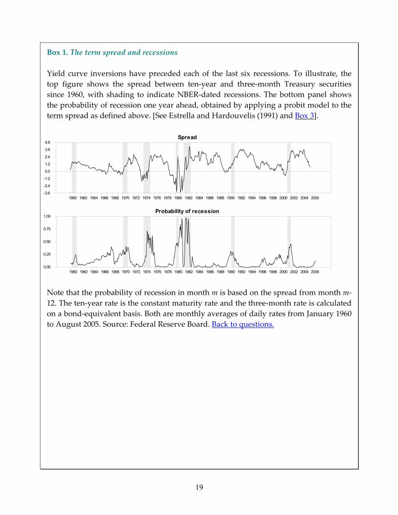
Box 1. The term spread and recessions  Yield curve  inversions have preceded each of  the  last six  recessions. To  illustrate,  the top  figure  shows  the  spread  between  ten‐year  and  three‐month  Treasury  securities since 1960, with shading  to  indicate NBER‐dated  recessions. The bottom panel shows the probability of recession one year ahead, obtained by applying a probit model to the term spread as defined above. [See Estrella and Hardouvelis (1991) and Box 3].  

Note that the probability of recession in month m is based on the spread from month m‐12. The ten‐year rate is the constant maturity rate and the three‐month rate is calculated on a bond‐equivalent basis. Both are monthly averages of daily rates from January 1960 to August 2005. Source: Federal Reserve Board. Back to questions.

Spread

1960 1962 1964 1966 1968 1970 1972 1974 1976 1978 1980 1982 1984 1986 1988 1990 1992 1994 1996 1998 2000 2002 2004 2006-3.6

-2.4

-1.2

0.0

1.2

2.4

3.6

4.8

Probability of recession

1960 1962 1964 1966 1968 1970 1972 1974 1976 1978 1980 1982 1984 1986 1988 1990 1992 1994 1996 1998 2000 2002 2004 20060.00

0.25

0.50

0.75

1.00

19

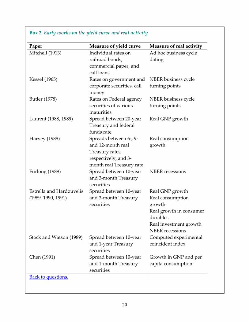
Box 2. Early works on the yield curve and real activity  Paper  Measure of yield curve  Measure of real activity Mitchell (1913)  Individual rates on 

railroad bonds, commercial paper, and call loans 

Ad hoc business cycle dating 

Kessel (1965)  Rates on government and corporate securities, call money 

NBER business cycle turning points 

Butler (1978)  Rates on Federal agency securities of various maturities 

NBER business cycle turning points 

Laurent (1988, 1989)  Spread between 20‐year Treasury and federal funds rate 

Real GNP growth 

Harvey (1988)  Spreads between 6‐, 9‐ and 12‐month real Treasury rates, respectively, and 3‐month real Treasury rate 

Real consumption growth 

Furlong (1989)  Spread between 10‐year and 3‐month Treasury securities 

NBER recessions 

Estrella and Hardouvelis (1989, 1990, 1991) 

Spread between 10‐year and 3‐month Treasury securities 

Real GNP growth Real consumption growth Real growth in consumer durables Real investment growth NBER recessions 

Stock and Watson (1989)  Spread between 10‐year and 1‐year Treasury securities 

Computed experimental coincident index 

Chen (1991)  Spread between 10‐year and 1‐month Treasury securities 

Growth in GNP and per capita consumption 

Back to questions.

20

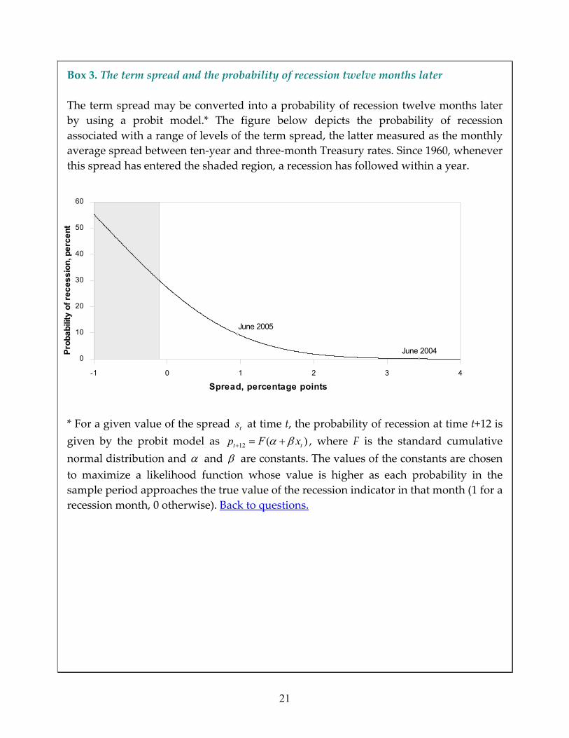
Box 3. The term spread and the probability of recession twelve months later   The term spread may be converted  into a probability of recession twelve months  later by  using  a  probit  model.*  The  figure  below  depicts  the  probability  of  recession associated with a range of levels of the term spread, the latter measured as the monthly average spread between ten‐year and three‐month Treasury rates. Since 1960, whenever this spread has entered the shaded region, a recession has followed within a year. 

* For a given value of the spread   at time t, the probability of recession at time t+12 is given  by  the  probit model  as 

ts

12 (t )tp F xα β+ = + , where  F  is  the  standard  cumulative normal distribution and α  and  β  are constants. The values of the constants are chosen to maximize  a  likelihood  function whose  value  is  higher  as  each  probability  in  the sample period approaches the true value of the recession indicator in that month (1 for a recession month, 0 otherwise). Back to questions.

Spread, percentage points

Prob

abili

ty o

f rec

essi

on, p

erce

nt

-1 0 1 2 3 4

0

10

20

30

40

50

60

June 2005

June 2004

21

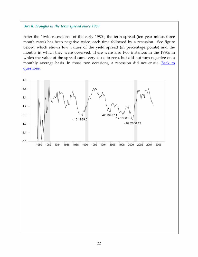
Box 4. Troughs in the term spread since 1989  After  the “twin  recessions” of  the early 1980s,  the  term  spread  (ten year minus  three month  rates) has been negative  twice,  each  time  followed by  a  recession.   See  figure below, which  shows  low  values  of  the  yield  spread  (in  percentage  points)  and  the months  in which  they were  observed. There were  also  two  instances  in  the  1990s  in which the value of the spread came very close to zero, but did not turn negative on a monthly  average  basis.  In  those  two  occasions,  a  recession  did  not  ensue.  Back  to questions.

 

1980 1982 1984 1986 1988 1990 1992 1994 1996 1998 2000 2002 2004 2006-3.6

-2.4

-1.2

0.0

1.2

2.4

3.6

4.8

-.16 1989:6.42 1995:11

.12 1998:9

-.69 2000:12

22

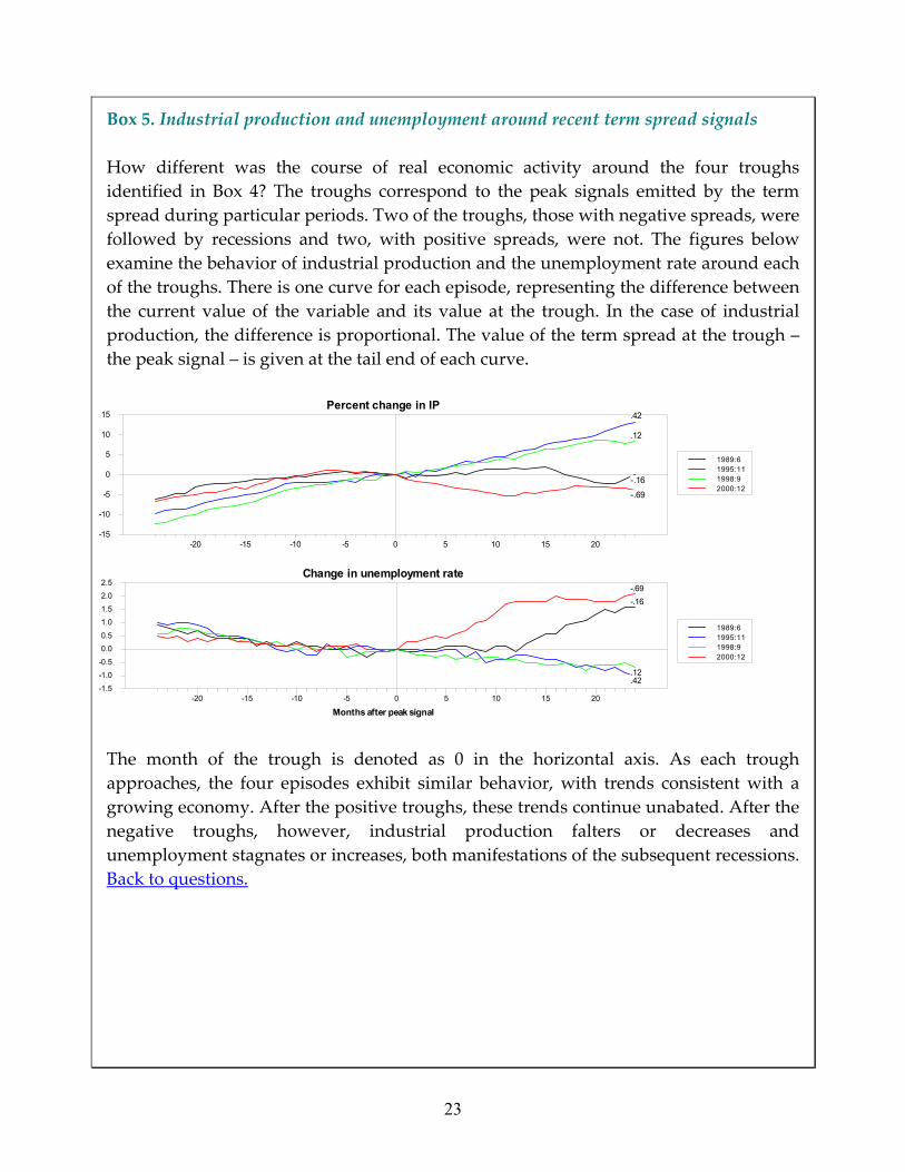
Box 5. Industrial production and unemployment around recent term spread signals  How  different  was  the  course  of  real  economic  activity  around  the  four  troughs identified  in Box  4? The  troughs  correspond  to  the peak  signals  emitted by  the  term spread during particular periods. Two of the troughs, those with negative spreads, were followed  by  recessions  and  two, with  positive  spreads, were  not.  The  figures  below examine the behavior of industrial production and the unemployment rate around each of the troughs. There is one curve for each episode, representing the difference between the  current value of  the variable and  its value at  the  trough.  In  the  case of  industrial production, the difference is proportional. The value of the term spread at the trough – the peak signal – is given at the tail end of each curve.  

The  month  of  the  trough  is  denoted  as  0  in  the  horizontal  axis.  As  each  trough approaches,  the  four  episodes  exhibit  similar behavior, with  trends  consistent with  a growing economy. After the positive troughs, these trends continue unabated. After the negative  troughs,  however,  industrial  production  falters  or  decreases  and unemployment stagnates or increases, both manifestations of the subsequent recessions. Back to questions. 

1989:61995:111998:92000:12

Percent change in IP

-20 -15 -10 -5 0 5 10 15 20-15

-10

-5

0

5

10

15

-.16

.42

.12

-.69

1989:61995:111998:92000:12

Change in unemployment rate

Months after peak signal-20 -15 -10 -5 0 5 10 15 20

-1.5-1.0-0.50.00.51.01.52.02.5

-.16

.42

.12

-.69

23