The Yield and Post-Yield Behavior of by - NASA purpose of this research is to study the yield and post-yield behavior of a thermoplastic polymer subjected to biaxial stress states

The Yield and Post-Yield Behavior

High-Density Polyethylene

by

M.A. Semeliss, Research Assistant

g. Wong, Research AssistantM.E. Turtle, Assistant Professor

of

Department of Mechanical Engineering, FU-10

University of Washington

Seattle, Washington 98195

Prepared for:

NASA-Langley Research Center

Grant No. NAG-I-974

Dr. W.S. Johnson, Program Monitor

May 1990

https://ntrs.nasa.gov/search.jsp?R=19900015903 2018-06-17T08:10:14+00:00Z

TABLE OF CONTENTS

ACKNOWLEDGEMENTS ..................................................................

CHAPTER 1: INTRODUCTION ...........................................................

Pul_pO Se o**,oo.oo,°o,o°oo,o°o.,,,.,ooooQ°o_o.o,o°.oooooooooooooo°o°..o...o .... °

CHAPTER 2: BACKGROUND INFORMATION .......................................

The Prediction of Yielding ..........................................................Definition of Yield Stress ..................................................Yield Criteria ................................................................

Isotropic Yield Criteria ............................................Anisotropic Yield Criteria .........................................

The Prediction of Post-Yield Behavior ............................................

Post Yield Behavior of Isotropic Materials ..............................Post Yield Behavior of Anisotropic Materials ...........................

CHAP'IER 3: EXPEKIMENTAL PROCEDURES ......................................Derivation of Test Matrix ...........................................................

Specimen Preparation ...............................................................Axial Load and Internal Pressure Control .........................................

Data Acquisition ......................................................................Summary of Test Procedure ........................................................

CHAPTER 4: DATA REDUCTION METHODS .........................................

Determination of Material Properties ..............................................Prediction of Yielding - Isotropic Model ..........................................Prediction of Yielding - Transversely Isotropic Model ..........................Prediction of Post Yield Behavior ..................................................

Power Law Models ..........................................................

Isotropic Form .....................................................Anisotropic Form ..................................................

Prandtl-Reuss Model .......................................................Lode Parameters ....................................................

CHAPTER 5: RESULTS AND DISCUSSION ..........................................Yield Predictions .....................................................................

Isotropic Models ............................................................Anisotropic Models .........................................................

Post Yield Predictions ...............................................................Power Law Model ..........................................................

Isotropic Form .....................................................Anisotropic Form ..................................................

Prandtl-Reuss Model ................................................................Calculation of the Lode Paramters ........................................Prandd-Reuss Predictions .................................................

Discussion of Pre- and Post-Yield Behavior .....................................

CHAFrI'ER 6: SUMMARY AND CONCLUSIONS ....................................

°oo

111

12

444

579

121319

2123253436

42x

4545465O525252545658

595959646565656969697090

92

ii

LIST OF REFERENCES ....................................................................

APPENDIX A: EXPERIMENTAL STRESSES AND STRAINS .....................

APPENDIX B: YIELD POINT DETERMINATION FOR ISOTROPIC ANDTRANSVERSELY ISOTROPIC MODELS .............................

APPENDIX C: STANDARD DEVIATION CaM.L-'ULATIONS .......................

95

98

116

134

oot

111

ACKNOWLEDGEMENTS

This research was supported through grant NAG-1-974 from the NASA-Langley

Research Center. The: authors wish to thank the Program Monitor Dr. W. S. Johnson for

his support and enthusiam. The many helpful discussions and suggestions of Drs. J. H.

Crews and C. E. Harris of NASA-Langely are also gratefully acknowledged.

CHAPTER 1: INTRODUCTION

There has been a rapid growth in the use of polymers and polymeric-based materials in

recent years, and there is every indication that this trend will continue. Of particular interest has

been the use of polymers as the matrix component in structural composite materials. Polymers

may be roughly categorized as being either thermosets or themoplastics. Both thermosets and

thermoplastics are comprised of long molecular chains. However, the molecular chains of

thermosets are highly cross-linked, forming an extensive three-dimensional molecular structure.

Conversely, thermoplastics do not form cross-links. One of the ramifications of this difference in

molecular structure is that once a thermoset polymer has been polymerized (i.e., once the cross-

links have been formed) the thermoset cannot be melted. On the other hand thermoplastics can be

readily melted and remolded by the application of heat and pressure. Most thermoplastics have

glass-transition and melting temperatures much lower than the glass-transition temperature of

thermosets, and thus thennoset resins have been used most often in structural composite materials.

However, recent advancc:s in polymer materials technology have resulted in a new generation of

high-temperature thermoplastic polymers which are better suited for engineering applications.

Examples of these new-generation thermoplastics include poly-ether-ether-ketone ("PEEK", with a

melting temperature of roughly 340°C) or a variety of polyimide resins (with a melting temperature

ranging from 230-350°C). Because of these thermal properties as well as the inherent toughness

and relative ease with which thermoplastics can be fabricated, recent research and developmental

efforts in structural coml_site materials have turned to thermoplastic-based matrices.

The expanding role of thermoplastic polymers in load-bearing structural applications has

prompted a need to develop a design methodology to predict the mechanical response of these

materials under complex loading conditions. In particular, prediction of yield and post-yield

2

behavioris of currenttechnicalinterest.At presentmostof thedesigntoolsandconceptsusedin

theanalysisof polymeric-basedmaterialsarebasedon thesameprinciples usedfor metalsand

metallicalloys. However,theatomic/molecularstructureof polymersisentirelydifferentfrom that

of metals. Metalsarecharacterizedby ahighlycrystallineatomicstructurewhereaspolymersare

characterizedby longmolecularchainsthatmaybeamorphousor semi-crystallineat themolecular

level. Since the macroscopicyield andpost-yield behaviorof any material is fundamentally

governedby its atomic/molecularmicrostructure,it is unlikely thatadesignmethodologyusedfor

metalswill applyequallywell to polymers.Therefore,it maybenecessaryto developnewdesign

methodologiesfor polymers,or to modify existingdesigntools that hadbeendevelopedfor use

with metals.

Purpose

The purpose of this research is to study the yield and post-yield behavior of a thermoplastic

polymer subjected to biaxial stress states. In particular, experimental results will be compared with

theoretical predictions based on classical plasticity theories previously applied to metals. Of

particular interest is whether the yield or post-yield behavior of thermoplastic polymers is

influenced by the hydrostatic stress component.

The material cho,,;en for study was high-density polyethylene. High-density polyethylene

has a melting temperature,, of roughly 130°C, and is not considered to be a potential matrix material

for use in structural composites. Polyethylene was selected because (1) it is a semi-crystalline

thermoplastic, and hence its post-yield behavior may be representative of the general class of

thermoplastic polymers, (2) it is readily available in the form of thin-walled tubes, and (3) it is very

inexpensive as compared to new-generation thermoplastics such as PEEK or polyimides, and

- 3

hencealargenumberof test_,; could be conducted at modest cost

The study involved plane stress problems where thin-walled tubes of high-density

polyethylene were tested tinder combined tensile axial loads and internal pressures at room

temperatures. A rather spea:ialized testing apparatus was developed during the study in order to

perform these tests. This testing system is now fully calibrated and operational, and will be used

to study the inelastic behavior of other new-generation thermoplastic resins of greater structural

interest during the coming _.,ear.

CHAPTER 2: BACKGROUND INFORMATION

THE PREDICTION OF YIELDING

Definition of the Yield Stress

Conceptually, the yield point of a material defines the transition from purely elastic to

elastic/plastic behavior. For some materials, the yield point is indicated by a sharp drop in stress in

a uniaxial stress-strain cu_e, followed by slowly increasing stress with increasing strain. In these

cases the near-discontinuity in stress makes identification of the yield stress very easy. For other

materials no such stress drop occurs, but instead the slope of the stress-strain curve gradually

decreases from an initial "elastic" value, which defines Young's modulus, to a lower value. In

these cases the identification of yielding becomes more problematic. A common method of

defining yield in this case is to use a permanent strain offset. For metals, this strain offset is

usually defined as 0.2% strain.

Defining yield in polymers involves complexities not normally encountered with metals.

Polymers are viscoelasti,: and therefore the measured yield stress is sensitive to the stress- or

strain-rate imposed. Researchers have attempted to def'me the yield stress of polymers in a variety

of ways. One method [Bowden and Jukes, 1972; Freire and Riley, 1980; Meats et al, 1969;

Whitfield and Smith, 1972] is identification of the point of load drop, as described above. Another

method [Carapellucci and Yee, 1986] is to perform a constant stress creep test, and to define yield

based upon the intersection of tangents drawn to the initial and f'mal portions of the resulting strain

versus time curve. Probably the most common method is to apply a monotonically increasing axial

load at a constant rate, and to define yielding on the basis of a strain offset. However, no standard

loading rate or strain offset has been established. Offset strains ranging from 0.3% strain [Caddell

5

and Woodliff, 1977; Raghava et al, 1973] to as high as 2% strain [ Ely, 1967; Pae, 1977] have

been used.

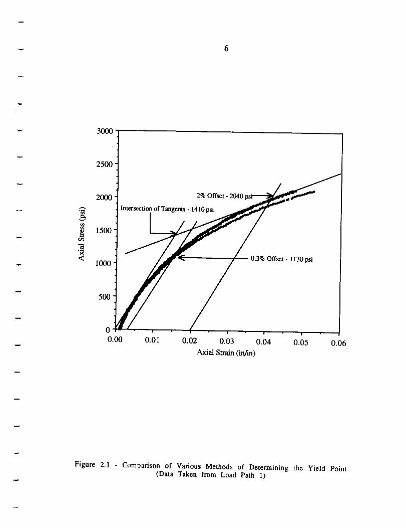
Obviously, the c_ifferent methods to determine yield result in distinctly different values of

measured "yield strength" for a given polymer. Figure 2.1 compares various methods used to

determine the yield strength of a polymer, and indicates that distinctly different values of the "yield

point" can be deduced from the same experimental data. The inconsistency in the definition of

"yielding" makes comparison of results obtained during different studies difficult. A standard

definition, such as exist:; for metals, needs to be adopted for use with polymers.

The method useM to define yielding during the present study will be discussed in detail in a

following section. At this point it is appropriate to note that yielding was defined on the basis of a

0.3% offset in the octatu,dral shear stress vs octahedral shear strain curve of polyethylene. A value

of 0.3% was selected because it is a widely used value of strain offset, at least within the polymers

technical community. Yielding was defined in terms of octahedral shear stress and octahedral

shear strain because this approach automatically accounts for biaxial loading effects. Also, all tests

were conducted under a constant rate in order to minimize rate effects. Specifically, the yield and

post-yield response of the polyethylene specimens was measured under a condition of constant

octahedral shear stress loading.

Yield Criteria

The yield criteria which have been developed for metals typically make the following

assumptions: (1) the initial compressive and tensile yield strengths are equal, (2) the hydrostatic

stress component does not contribute towards yielding (i.e., the deviatoric stress component

6

"3<

3°l2500

2000

1500

I000

5OO

0

0.00

2% Offset - 2040

Inters_,,ction of Tangents - 1410 psi

0.3% Offset - 1130 psi

0.01 0.02 0.03 0.04 0.05 0.06

Axial Swain (in/in)

Figure 2.1 Comparison of Various Methods of Determining the Yield Point(Data Taken from Load Path 1)

7

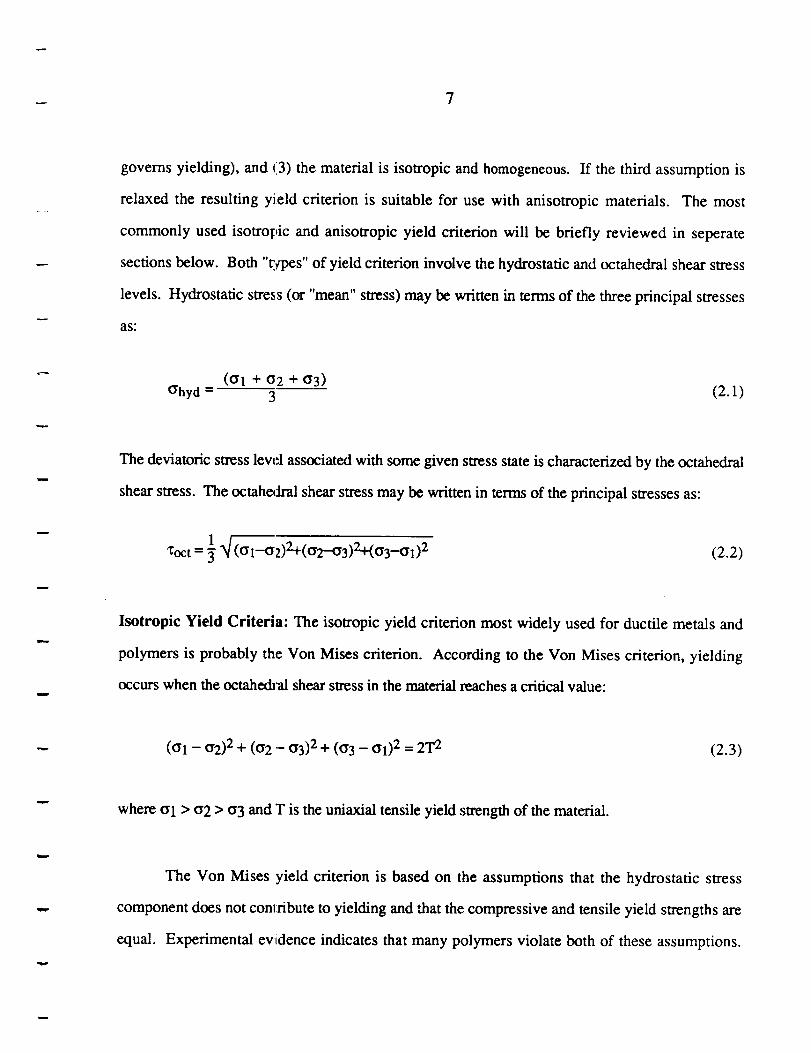
governs yielding), and (3) the material is isotropic and homogeneous. If the third assumption is

relaxed the resulting yield criterion is suitable for use with anisotropic materials. The most

commonly used isotropic and anisotropic yield criterion will be briefly reviewed in seperate

sections below. Both "types" of yield criterion involve the hydrostatic and octahedral shear stress

levels. Hydrostatic stress (or "mean" stress) may be written in terms of the three principal stresses

as:

(_1 +02+G3)ffhyd = 3-- (2.1)

The deviatoric stress level associated with some given stress state is characterized by the octahedral

shear stress. The octahe&ral shear stress may be written in terms of the principal stresses as:

1 (a_--_l _a 2)2+(0.2...a3)2+(O.3_G1) 2'COCt ---- (2.2)

lsotropic Yield Criteria: The isotropic yield criterion most widely used for ductile metals and

polymers is probably the Von Mises criterion. According to the Von Mises criterion, yielding

occurs when the octahe&al shear stress in the material reaches a critical value:

((sl - a2) 2 + (ts2 - 03) 2 + (U3 - 01) 2 = 2"I`2 (2.3)

where t_1 > _2 > a3 and T is the uniaxial tensile yield strength of the material.

The Von Mises yield criterion is based on the assumptions that the hydrostatic stress

component does not conn'ibute to yielding and that the compressive and tensile yield strengths are

equal. Experimental evidence indicates that many polymers violate both of these assumptions.

8

Thatis,polymersdo in generalhavedistinctlydifferentcompressiveandtensileyield strengthsand

furthermoretheir yield behavioris significantly influencedby the hydrostaticstresslevel. For

example,Christiansen,Baer,andRadcliffe [ 1971]foundthattheyield strengthof polycarbonate,

polyethyleneterephthalate,polychloro-trifluoroethylene,andpolytetrafluoroethyleneall increased

with increasinghydrostaticpressure.Mears,PacandSauer[1969]havereportedsimilarpressure-

dependentyield behaviorsfor polyethyleneandpolypropylene.The sameconclusionshavebeen

reachedfor a varietyof otherpolymersduringstudiesby Ainbinderet al [1965],PaeandMears

[1968],Sardaret al ([1968], andSpitzig [1979]. This experimentalevidenceindicatesthat yield

criteriawhichassumethatthehydrostaticstresscomponentdoesnot influencetheyield behavior,

and/orwhich assumethat the initial compressive and tensile yield strengths are equal are not

applicable for use with txflymers.

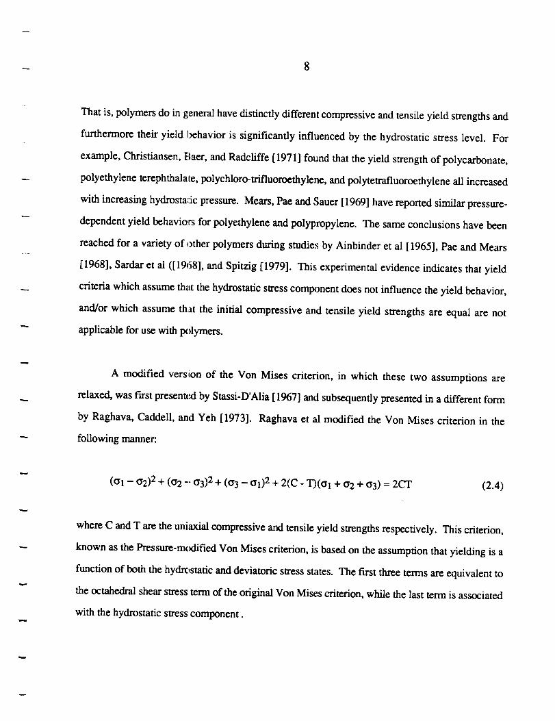
A modified version of the Von Mises criterion, in which these two assumptions are

relaxed, was fast present_'.d by Stassi-D'Alia [ 1967] and subsequently presented in a different form

by Raghava, Caddell, and Yeh [1973]. Raghava et al modified the Von Mises criterion in the

following manner:

(t_l - tJ2) 2 + (t_2 -- t_3)2 + (t_ 3 - t_l)2 + 2(C - T)(t_l + t_2 + _3) = 2CT (2.4)

where C and T are the uniaxial compressive and tensile yield strengths respectively. This criterion,

known as the Pressure-modified Von Mises criterion, is based on the assumption that yielding is a

function of both the hydrostatic and deviatoric stress states. The first three terms are equivalent to

the octahedral shear stress term of the original Von Mises criterion, while the last term is associated

with the hydrostatic stress component.

9

Note that effect.,; of hydrostatic stress and differences in compressive/tensile strength are

not independent in the Pressure-modified Von Mises criterion. That is, if the compressive and

tensile yield strengths of a material are equal then the hydrostatic stress term disappears and the

Pressure-modified Von Mises criterion reduces to the original Von Mises criterion. It is interesting

to note that a similar interdependence between tensile/compressive yield strengths and hydrostatic

effects has been demonstrated for some metals. Spitzig, Sober, and Richmond [1976] have shown

that some sintered powder materials (e.g., sintered iron) exhibit significant differences in

compressive and tensile yield strength, and also that the yield behavior of these metals is influenced

by the hydrostatic stress component. Similar conclusions were reached by Betten, Frosch, and

Borrmann [1982] for the case of quenched and tempered steels.

The yield behavior of polymers has been compared to both the Von Mises and Pressure-

modified Von Mises Criterion. Polymers which have been studied include acrylics [Ely ; 1967],

polyester mixtures [Freire and Riley ;1980], and polycarbonate, polyvinylchloride, and

polyethylene [Raghava and Caddell, 1973; Raghava et al, 1973]. In all cases the Pressure-

modified Von Mises criterion was a better predictor of yield than the original Von Mises criterion,

indicating that the yield n_.sponse of these polymers is sensitive to the hydrostatic stress level.

Anisotropic Yield Criteria: Anisotropic materials possess different material properties in

different directions. Until recently, most research on the yield behavior of materials has focused

on isotropic models. However, many materials are anisotropic. In addition, when shaped by

manufacturing processes such as rolling or extrusion even materials which are initially isotropic

may become oriented at the atomic/molecular level and therefore become anisotropic at the

macroscale. This is particularly true of polymers since they are composed of long molecular chains

10

whichcaneasilybecome:orientedin onedirection,resultingin apolymerwith distinctly different

stiffnessesandstrengthsin differentdirections.

Thecriterionusedmostoftento model the behavior of anisotropic materials is the Tsai-Hill

yield criterion. Hill [1950] developed this criterion by selecting a form which would reduce to the

Von Mises criterion if file yield strengths were the same in all directions. Tsai has subsequently

applied this theory to composite materials, and the resulting theory is now known as the Tsal-Hill

yield criterion. It can be written in the following manner in terms of the principal stresses t: l, t:2,

and a3:

H(t_l - tJ2) 2 + F(t_2 - t_3) 2 + G(a3 - t_l) 2 = 1

1 1 1with: H+G- H+F- G+F-

T12 T2 2 T3 2

(2.5)

Since the material is ani.,;otropic, the coefficients in the equation are functions of the tensile yield

strengths in the 1-, 2- anti 3- directions, T1, T2 and T3 respectively. If the material is transversely

isotropic, then T2 and T3 are equal and consequently G is equal to H. The Tsal-Hill yield criterion

is related to the maximum shear which exists in each principal plane; it includes no linear terms

which would represent the hydrostatic stress level, and also ignores any differences in initial

compressive and tensile yield strengths. Stassi-D'Alia [1969] modified the Tsai-Hill criterion to

include these factors, and Caddell, Raghava, and Atldns [1973] proposed a similar yield criterion

at a later date. The Pressure-modified Tsai-Hill criterion, as it is sometimes known, is defined as

follows:

H(Ol - 02) 2 + F(tI2 - (I3) 2 + G((_3 - 01) 2 + Kltll + K2t_2 + K3(_3 = 1 (2.6)

11

1 1 1with H+G-c1TI H+F-c2T2 G+F-c3T3

C2- T2 _C3-T3K1 C1- T1 K2- K3- C1T1 C'2_I'2 =--C3T3

The Compressive and tensile yield strengths in the 1-, 2-, and 3- directions are denoted by C1, T1,

C2, T2, C3, and T3. If the material is transversely isotropic then C2 and T2 are equal to C3 and

T3, and therefore, G = H. If the compressive and tensile strengths are equal, Eq (2.6) reduces to

the original Tsai-Hill criterion, and if material properties are the same in all directions, it further

reduces to the original Von Mises critedon.

The few experir.aental studies which have been undertaken to investigate the yield behavior

of anisotropic polymer:; seem to validate the Pressure-modified Tsai-Hill yield criterion. Studies

by Rider and Hargreaves [1969] and Shinozaki and Groves [1973] followed methods suggested

by Hill in which the change in the tensile and compressive yield strengths of oriented polymer

sheets was measured as a function of the angle of orientation 0. Caddell and Woodliff [1977]

conducted a series of tests using highly anisotropic specimens of polycarbonate, polyethylene, and

polypropylene. The test specimens were oriented by applying a tensile load to a specimen until a

stable neck had formed. The final test specimens were then machined out of these necked regions.

A good correlation between experiment and theory was reported. Carapellucci and Yee [1986] also

conducted tests on anisotropic polycarbonate specimens and reported good agreement. Hence, it

appears that the yield behavior of anisotropic polymers is significantly affected by the hydrostatic

stress level.

12

THE PREDICTION OF POST-YIELD BEHAVIOR

Post-yield behavior typically involves large deformations, such that the familiar definitions

of conventional "engineering" stress and strain no longer apply. Conventional engineering stress

and engineering strain e ]nay be converted to true stresses s and true strains e as follows:

s = _(_+ 1)(2.7)

e = ln(E+l) (2.8)

A true stress-true strain curve is often called a plastic "flow" curve because it gives the

stress which causes the material to flow plastically for any given strain. Post-yield theories are

typically developed in terms of the true stress and true strain, and in this report true stress and true

strain will be used to describe the post-yield behavior of polyethylene.

The post-yield theories considered during this study will be briefly reviewed below. Both

isotropic and anisotropic materials will be discussed. It is appropriate to note that, in contrast to

the yield criterion reviewed above, all existing post-yield criteria assume material incompressibility

during plastic flow. The possibility that the flow behavior of polymers is influenced by the

hydrostatic stress level has apparently not yet been addressed within the technical community.

13

Post Yield Behavior of lsotropic Materials

The assumption that plastic deformations are independent of the hydrostatic stress level

leads to the conclusion that the volume of a solid remains constant during plastic flow. Therefore,

during plastic flow the true strains are related by:

el + e2 + e3 = 0 (2.9)

Equation (2.9) represents the "constancy of volume" assumption. Note that if v = 1/2, then a

similar relationship holds for engineering swains:

el +e2 +e3 = (l-2v)(a 1 + a2 + t_3)/E =0 (whenv = 1/2) (2.10)

For many metals undergoing plastic deformation induced by a uniaxial stress, the flow curve can

be expressed by the simple power law relation, also known as the Ludwik expression:

s = Syield + Men (2.11)

where Syield is the true stress at yield, M is the strength coefficient and n is the strain hardening

exponent. This equation is only valid for isotropic materials and is defined from the onset of

plastic flow to the maximum load at which the specimen begins to neck. Equation (2.11) provides

a simple mathematical expression to describe the post-yield flow curves of a material if constants M

and n are known.

14

Equation(2.11) is appropriatefor useunderuniaxial loadingconditions. In a complex

stateof stressandstrainit is moreusefulto relateinvariantfunctionsof truestressandtruestrain.

The invariant functions mostfrequentlyusedto describeplastic deformationof metalsare the

effectivetruestressandeffectivetruestrain[Dieter,1986].Theeffectivetruestressis definedasa

functionof theprincipaltruestresses:

11

_=_[(Sl-S2)2+ (S2-S3)2+(S3-Sl)212(2.12)

Theeffectivetruestrainisdefined as a function of the principal true strains:

g = --_ [(el-e2) 2 + (e2-e3) 2 + (e3-el)21 _ (2.13)

The power law relation ca:a now be expressed in the form of effective true stress and effective true

strains:

s = Syield + MEn(2.14)

An assumption implied by Equation (2.14) is that the flow curve is independent of the hydrostatic

or mean stress component. That is, the post-yield behavior is assumed to be governed exclusively

by the deviatoric stress tensor.

The power law expressions (i.e., either Eqs. 2.11 or 2.14) provide a simple mathematical

expression to describe the flow curves of a material, and the power law formulation has been

15

widely applied because of this simplicity. However, these relations are entirely empirical and

deviations from the power law are frequently observed.

More rigorous expressions to describe the post-yield behavior of a material have been

developed. Two such systems of equations are the Levy-Mises and Prandtl-Reuss equations. In

either case two fundaraental assumptions are made: it is assumed that the material is elastic-

perfectly plastic, and further, it is assumed that the incremental change in plastic true strain induced

by an increase in true sla'ess is proportional to the total stress deviator, rather than the incremental

change in the stress deviator. The elastic strains are neglected in the Levy-Mises equation, and

thus the Levy-Mises equations are only applicable when large plastic deformations occur such that

the elastic deformations can be entirely neglected. The Prandlt-Reuss equations include both elastic

and plastic deformations. In the present study the elastic deformations could not be neglected and

hence the Prandtl-Reuss equations were applied, as further described below.

Reuss assumed that the plastic true strain-increment, at any instant of loading, is

proportional to the instantaneous stress deviation such that:

s'l s'2 s'3

where de p are the plastic principal true strain increments, sl are the deviatoric true stress

components, and d_ is a non-negative constant of proportionality which is not a material constant

but rather varies throughout the stress/strain history.

16

Equation (2.15) implies that the incrementalplastic strainsdependon the total current

deviatoricstressesandnoton theincrementalchangein deviatoricstresses.It is alsoimplied that

the principal axesof stressandplastic strainincrementscoincide. Again, the hydrostaticstress

componentassumesno rolein theplasticdeformationof thematerial.

For a givendirectionthetotalstrainincrementdet is definedasthesumof theplasticdeP

and elastic dee strain increments:

de_ = deip +dee (2.16)

The plastic strain increment deP is given by Equation (2.15), and hence [S later, 1977]:

deip = s' dK- 3 s ] d_, 2s- H (2.17)

where g is the effective true stress defined in Equation (2.12) and H (also known as the "plasticity

modulus") is the slope of the effective true stress-plastic strain curve. The elastic strain incremente

dei is dependent on both the deviatoric and hydrostatic stress components:

de e -2-G+dS_ _l_l_,v) dShyd (2.18)

where E is the Young's modulus, v is the Poissons ratio, and G is the shear modulus. The shear

modulus is related to Young's modulus and Poissons ratio:

17

G

E

2(1+v)

(2.19)

Combining Equations (2. lq') and (2.18) gives the total strain increments for a given direction i:

t 3 s'i d-g ds_ (1-2v) A,,. (2.20)

dei - 2 s--H + -_--_- + _ u_ny

Equation (2.20) is the Prandtl-Reuss relation applicable for initially isotropic materials to describe

post-yield stress-strain behavior.

A method of experimentally verifying whether it is appropriate to apply the Prandtl-Reuss

system of equations to a given material was developed by Lode (1926). Lode introduced two

parameters, I,t and v, known as the I.xxie stress and plastic strain parameters respectively:

2s2 - Sl - s_- Sl - s3

(2.21)

In Equation (2.21), the stresses are the total principal stresses and the strains are the plastic portion

of total principal strains defined as"

Cp = e t_ e e(2.22)

where e t and ee are the total and elastic principal strains respectively.

18

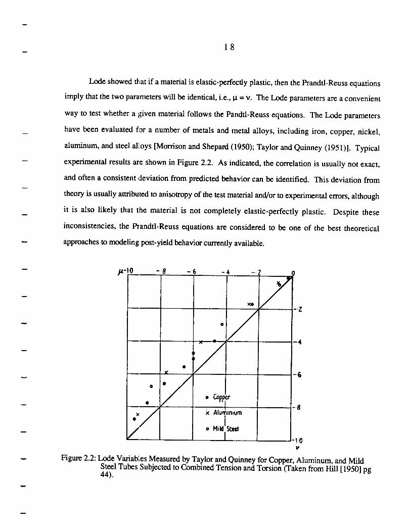
Lode showed that if a material is elastic-perfectly plastic, then the Prandtl-Reuss equations

imply that the two parameters will be identical, i.e., la = v. The Lode parameters are a convenient

way to test whether a given material follows the Pandtl-Reuss equations. The Lode parameters

have been evaluated for a number of metals and metal alloys, including iron, copper, nickel,

aluminum, and steel ali_oys [Morrison and Shepard (1950); Taylor and Quinney (1951)]. Typical

experimental results are shown in Figure 2.2. As indicated, the correlation is usually not exact,

and often a consistent deviation from predicted behavior can be identified. This deviation from

theory is usually attributed to anisotropy of the test material and/or to experimental errors, although

it is also likely that the material is not completely elastic-perfectly plastic. Despite these

inconsistencies, the lhandtl-Reuss equations are considered to be one of the best theoretical

approaches to modeling post-yield behavior currently available.

o

/ X Alumin,umo Hikl St:_

"I0IP

Figu__ 2.2: Lode Variables Measured by Taylor and Quinney for Copper, Alun'_num, and MildSteel Tubes Subjectedto Combined Tension and Torsion (Taken from Hill [ 1950] pg44).

19

Post-Yield Behavior of Anisotropic Materials

An anisotropic folm of the power law was applied to polyethylene during the present

study. The effective true ,;tress and effective true strain for istropic materials have been def'med in

Equations (2.12) and (2.13). These definitions no longer apply for anisotropic materials. Hill

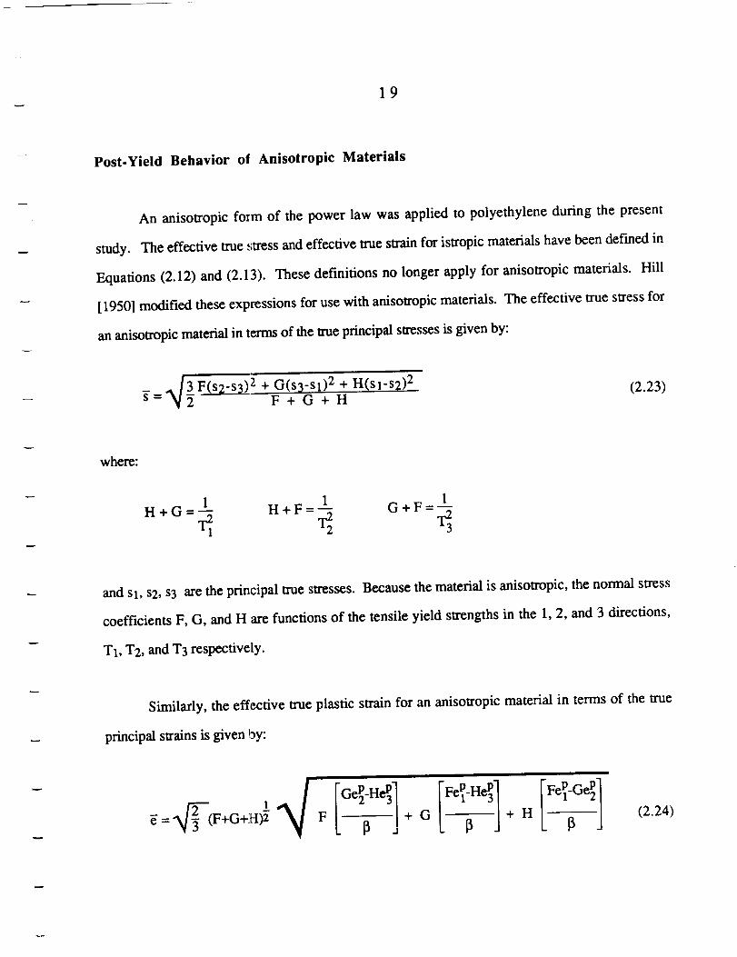
[1950] modified these expressions for use with anisotropic materials. The effective true stress for

an anisotropic material in terms of the true principal stresses is given by:

q3 F(s2-s3) 2 + G(s3-sl) 2 + H(sl-s2) 2s= 2 F+G+H(2.23)

where:

H+G---1 H+F- 1 G+F- 1

and Sl, s2, s3 are the principal true stresses. Because the material is anisotropic, the normal stress

coefficients F, G, and H are functions of the tensile yield strengths in the 1, 2, and 3 directions,

T1, T2, and T3 respectively.

Similarly, the effective true plastic strain for an anisotropic material in terms of the true

principal strains is given lay:

+G +H (2.24)

2 0

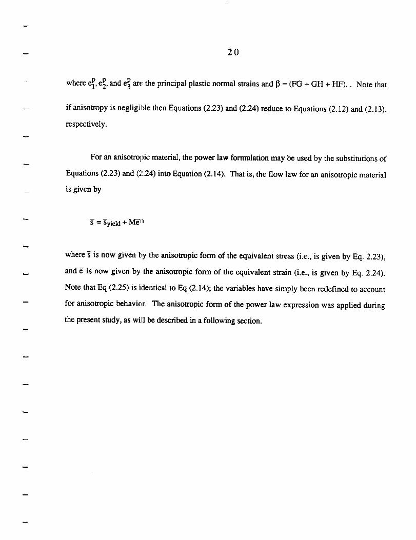
whereelP,ep.and e_ ar,.' the principal plastic normal swains and 13= (FG + GH + HF).. Note that

if anisotropy is negligible then Equations (2.23) and (2.24) reduce to Equations (2.12) and (2.13),

respectively.

For an anisotropic material, the power law formulation may be used by the substitutions of

Equations (2.23) and (2.24) into Equation (2.14). That is, the flow law for an anisotropic material

is given by

S = Syield + M-_-I'I

where g is now given by the anisotropic form of the equivalent stress (i.e., is given by Eq. 2.23),

and _- is now given by the anisotropic form of the equivalent strain (i.e., is given by Eq. 2.24).

Note that Eq (2.25) is identical to Eq (2.14); the variables have simply been redefined to account

for anisotropic behavior. The anisotropic form of the power law expression was applied during

the present study, as will be described in a following section.

CHAPTER 3 - EXPERIMENTAL PROCEDURES

In this study thin-walled tubes of high-density polyethylene were subjected to

monotonically increasing axial loads and internal pressures. This biaxial loading produced both

hoop and axial stresses within the walls of the specimen. Loading was increased proportionaly at

user-specified rates, and the yield and post-yield response of the specimen was monitored

throughout each test.

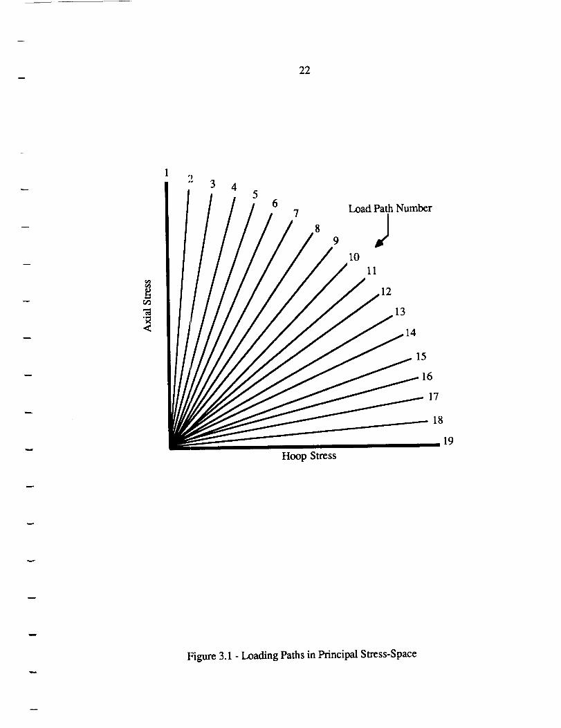
Due to symmetry the axial and hoop stresses were the principal stresses in all cases. The

axial and hoop stresses induced during a given test therefore def'me a radial "load path" in principal

stress space. The load paths used during the present study are summarized in Figure 3.1. A total

of 57 seperate tests were planned, involving three repeated tests along each of 19 load paths. The

load paths are oriented at five degree increments in the first quadrant of principal stress space.

The yield behavior of polyethylene is highly rate-dependent. As discussed in the preceding

chapter, in most yield- and post-yield criterion it is assumed that inelastic behavior is governed by

the octahedral shear stress. Therefore a constant octahedral shear stress rate was maintained during

all tests in order to minimize rate effects between individual tests and load paths. Note that

although the octahedral shear stress rate remained constant from test-to-test, the hydrostatic stress

rate, axial loading rate, and internal pressure rate all varied considerably from one load path to the

next.

22

1r,¢)

24

56

7 Load Path Number

, J9

/10 11

/G/ _12

17

Hoop Stress

18

19

Figure 3.1 - Loading Paths in Principal Stress-Space

23

Derivation of Test Matrix

The axial load (L) was increased at a rate of kl and the internal pressure (P) was increased

at a rate of k2. Therefore at time t:

L = klt (3.1)

P = k2t (3.2)

Under this loading condition, the stresses induced in the walls of the tube are:

t "kl )OAXIAL=OI=_(-_ + k2r (3.3)

OHOOP = 02 = _ c (3.4)

1O_,DtAL = - _ k2t = 0

with: r = average radius of tube

c = wall thickness

(3.5)

Note that the radial stress has been equated to zero. This is an appropriate assumption for thin-

walled tubes, since the radial stress is typically an order of magnitude less than the hoop and axial

stresses.

24

Normally, "o1" denotes the algebraically greatest principal stress, "02" the intermediate

principal stress, and "_3" the algebraically smallest principal stress. However, for purposes of

consistent identification this convention was ignored in this study. Instead, "o1" was used to

denote the axial stress, and "02" was used to denote the hoop stress, even though along some load

paths the hoop stress was in fact the algebraically greatest principal stress.

Substituting Ecls (3.3) and (3.4) into Eqs (2.1) and (2.2), the octahedral shear stress and

hydrostatic stress at any time t are given by:

t A /'_k_l 2

'toot = _ "_/-'_!r--_-- + 6k22r 2 (3.6)

t /k_z _- k2r)O'hyd = _ _3xr (3.7)

The slope M of any load path shown in Figure 3.1 can be expressed as:

- _2 - 2x -2r2 + rcr2 (3.8)

The combination of load rates kl and k2 which produce a desired slope M are given by:

kl = k2_r 2 (2M-I)(3.9)

Finally, given a desired octahedral shear stress rate, (Xoct/t), and slope M, the required axial load

rate and internal presstm: rate are given by:

25

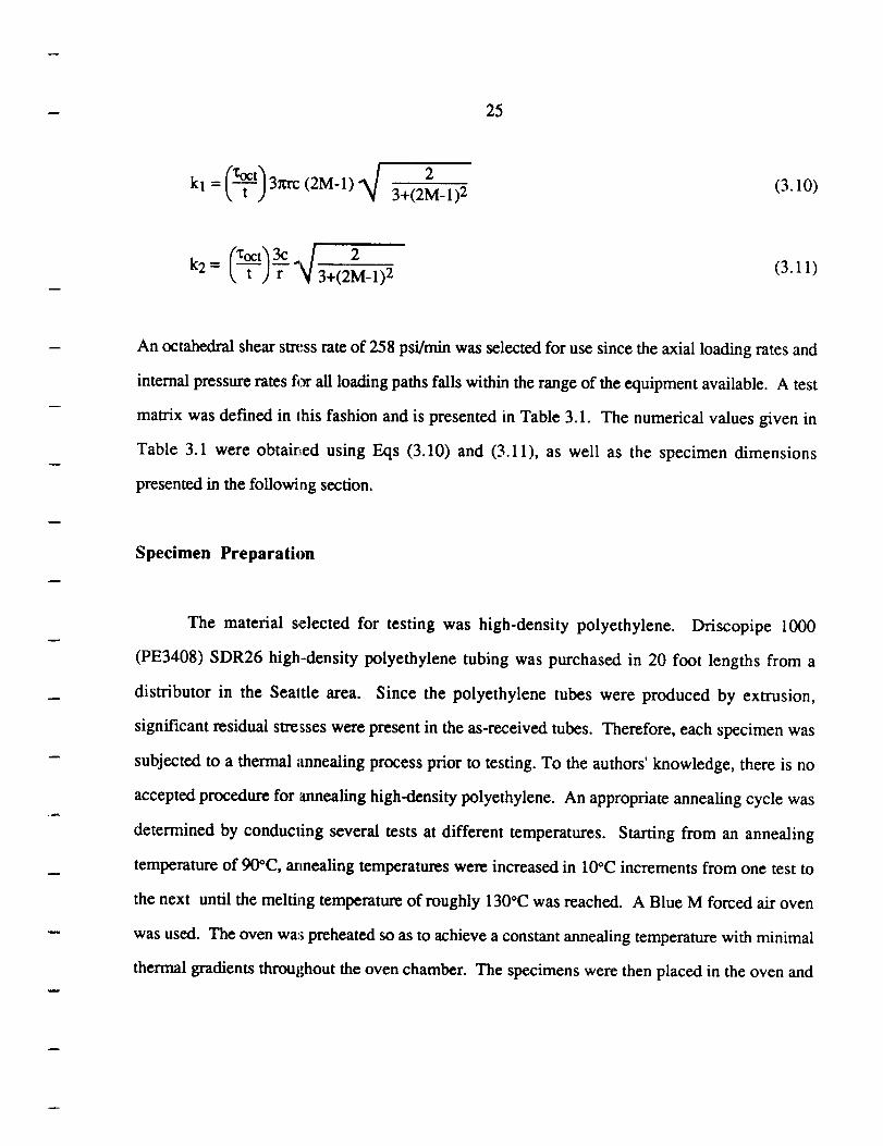
kl = 3_'rc(2M-l) 3+(2M_1)2 (3.10)

3+(2M_1)2 (3.11)

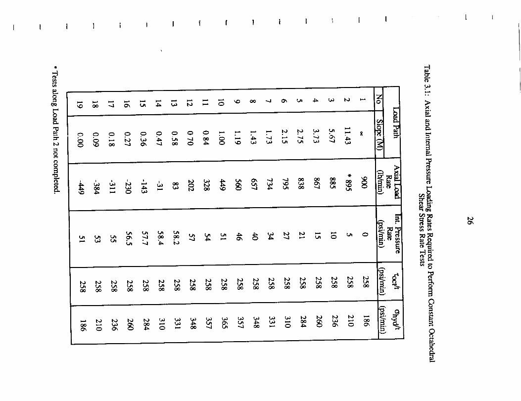
An octahedralshearsm;ssrateof 258psi/minwasselectedfor usesincetheaxial loadingratesand

internalpressureratesfi_rall loadingpathsfalls within therangeof theequipmentavailable.A test

matrix wasdefined in this fashion and is presented in Table 3.1. The numerical values given in

Table 3.1 were obtair, ed using Eqs (3.10) and (3.11), as well as the specimen dimensions

presented in the following section.

Specimen Preparation

The material selected for testing was high-density polyethylene. Driscopipe 1000

(PE3408) SDR26 high-density polyethylene tubing was purchased in 20 foot lengths from a

distributor in the Seattle area. Since the polyethylene tubes were produced by extrusion,

significant residual stresses were present in the as-received tubes. Therefore, each specimen was

subjected to a thermal _mnealing process prior to testing. To the authors' knowledge, there is no

accepted procedure for annealing high-density polyethylene. An appropriate annealing cycle was

determined by conducling several tests at different temperatures. Starting from an annealing

temperature of 90°C, annealing temperatures were increased in 10°C increments from one test to

the next until the melting temperature of roughly 130°C was reached. A Blue M forced air oven

was used. The oven wa:_ preheated so as to achieve a constant annealing temperature with minimal

thermal gradients throughout the oven chamber. The specimens were then placed in the oven and

] i i I i [ I I I I I I L L

,X-

,-]('D

0

0

Z0

I,n-'

,-]

oo

_.._o

:::s.TJ')

t_

27

annealed for one hour. The oven was then turned off and the specimens were slowly furnace

cooled over approximately 10 hrs.

The effect of anneal:mg temperatures was evaluated by means of a destructive sectioning

technique. A 1 inch wide strip was removed along the length of a 12 inch tube to evaluate axial

residual stresses. For the hoop direction, a 1-1/2 inch long "ring" specimens was cut from the

tube, and a 1-1/2 wide section (corresponding to a 20 ° arc) was cut out of the circumference of this

ring. After a period of 72 hours (to allow for any time-dependent response to develop) the strip

and ring specimens were examined to determine whether any deformations had occurred.

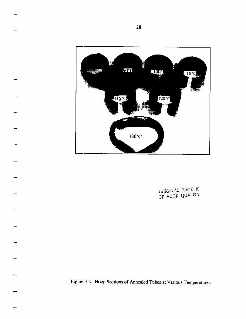
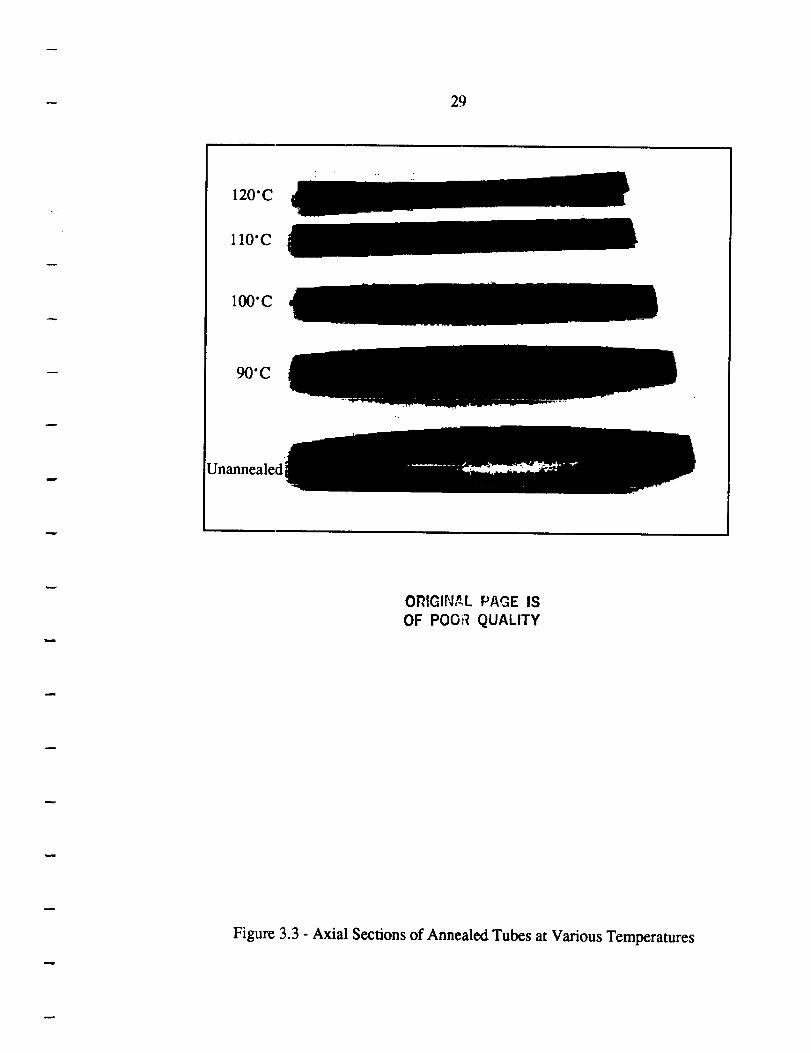
It was found that large residual stresses existed in the tubes in the as-received condition.

Compressive residual stresses existed in the hoop direction, while axial residual stresses were

probably compressive at the outer diameter and tensile at the inner diameter. Figures 3.2 and 3.3

show the results of the various annealing temperatures on hoop and axial residual stresses. Note

that at 130°C, the specimen had been extensively deformed by the annealing process, which

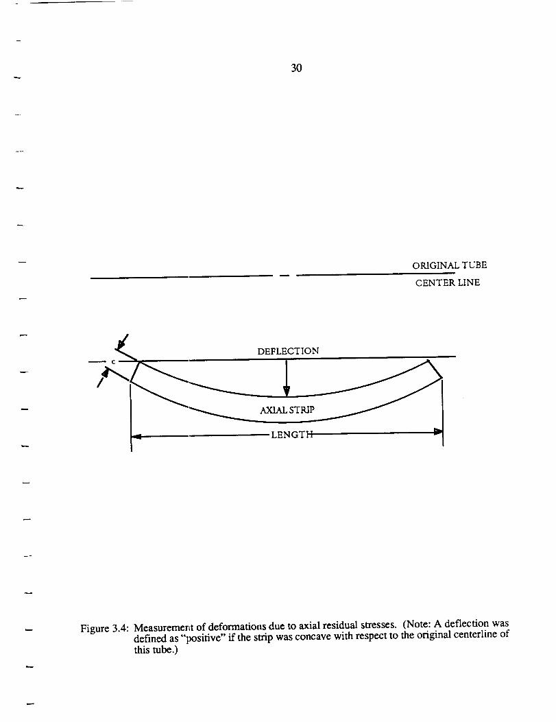
indicated that the melting temperature had been reached. For the axial direction, the amount of

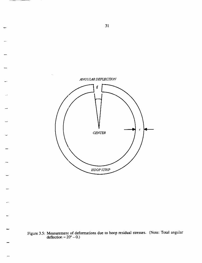
deflection from the center of the strip was measured as shown in Figure 3.4. For the hoop

direction, the angle of deflection from the center of the tube was measured as shown in Figure

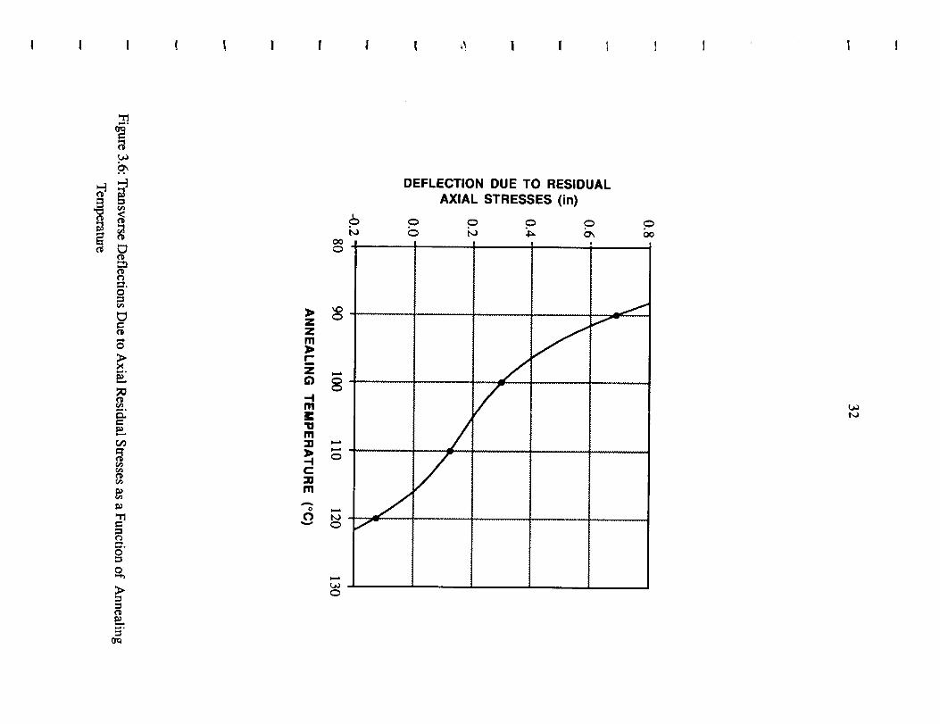
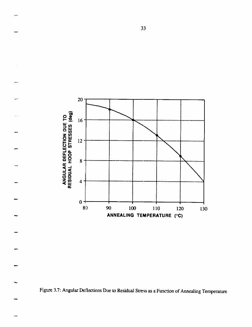
3.5. Measured deformations were plotted functions of annealing temperature, and the results are

summarized in Figure 3.6 and 3.7. The results show that deformation of the axial strip was

minimized using an annealing temperature of approximately 115°C. However, higher annealing

temperatures resulted in a algebraic sign change (i.e., a reversal in the curvature of the strip),

indicating that axial residua_ stresses may still have existed in the tubes following an anneal at

115°C. Furthermore, the hoop deformations were not completely eliminated even at annealing

temperatures approaching the melting temperature of polyethylene.

28

--,'"_'._ PAGE IS, _m l "It

OF POOR QU _'-'''g

Figure 3.2 - Hoop Sections of Annealed Tubes at Various Temperatures

29

120"C

110"C

lO0"C

90"C

Unannealed

OnlG!NAL PAGE IS

OF POOR QUALITY

Figure 3.3 - Axial Sections of Annealed Tubes at Various Temperatures

30

ORIGINAL TUBE

CENTER LINE

DEFLECT IO N

AXIAL STRIP

LENGTI I

Figure 3.4: Measurement of deformations due to axial residual stresses. (Note: A deflection wasdefined as "positive" if the strip was concave with respect to the original centerline of

this tube.)

31

ANGULAR DEFLECTION

f

CENTER

HOOP STRIP

Figure 3.5: Measurement of deformations due to hoop residual stresses.deflection = 20 ° - 0.)

(Note: Total angular

I I I ( ! I I I I ,_ I I I I I :' 1 I

_F

U

0

8

P_..

0

P_._,,J0

Z-

--Im

DEFLECTION DUE TO RESIDUAL

AXIAL STRESSES (in)

.o o .o .o

i

"Om

.-IC

m

- Z

/

0

33

oI"LU

_W_JZ_

ul

llc

20

A

oo_, 16

12

8 r

0

80 90 100 110 120 130

ANNEALING TEMPERATURE (°C)

Figure 3.7: Angular Deflections Due to Residual Stress as a Function of Annealing Temperature

34

The annealingtreatment finally selectedfor useconsistedof a 2 hour anneal at 115°C

followed by a 10 hr furnace cooling. It is believed that this annealing treatment minimized, but

perhaps did not completely eliminate, residual stresses present in the as-received tubes.

Specimens were cut frcm "parent" tubes in 15-1/2 inch lengths and annealed. Specimen

dimension measurements were; taken on six different sections of the annealed tubes in order to

determine average values. The average radius of the annealed tubes was 1.698", and the average

wall thickness was 0.157".

Axial Load and Internal Pressure Control

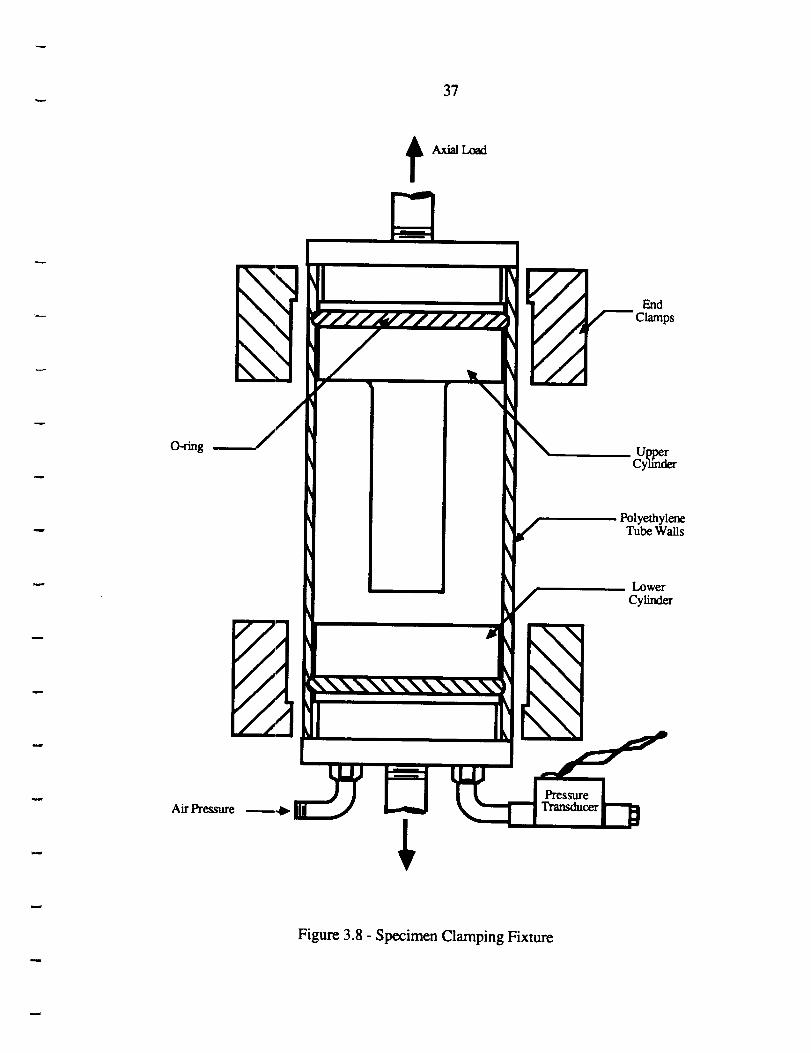
Figure 3.8 shows the fixture used to apply axial loads and internal pressures to the tubular

specimens. The specimens were mounted to two aluminum cylinders. The upper cylinder

extended into the specimen in order to reduce the volume of air required to pressurize the

specimen, which decreased the energy released in the event of catastrophic specimen failure. Two

ports were machined in the lower cylinder. One was the supply port for the pressurized air from a

bottled air cylinder and the o,aaer was the pressure transducer port for measuring internal pressures.

The tube specimens were seated on a shoulder machined in each aluminum cylinder. An O-

ring was used to insure proper pressurization with no leakage. After seating the tube on the

shoulder of each cylinder end, an aluminum clamp was attached at each end to firmly seal the tube

and cylinder surfaces. The clamp also helped prevent slippage of the tubes during testing by

pressing the specimen wall s into the machined step of the cylinders, thus increasing the friction

force between the mating surfaces of the tube and cylinder.

35

Axial loadswereappliedusinganMTS electrohydraulicfatiguetestingmachineconsisting

of a Model 308.01loading frame,a hydraulic cylinder andpump,a Model 442 control unit, a

Model 410 digital function generator,andaTransducerInc. Model WTC-FF42-CS-10K10kip

loadcell. A TektronixModel221360MHz oscilliscopewasusedto monitor andverify theaxial

loading. Figure3.9 illustratestheloadingframealongwith theloadcell andspecimen.

TheMTS framewasusedto applyamonotonicallyincreasingaxial loadat auser-specified

rate. Therequiredaxial loadingrateshavebeenpreviouslylistedin Table 3.1. Theappliedload

ratewasmonitoredthroaghouteachtest,andwasmaintainedto within +5% of the desired load

rate in all cases.

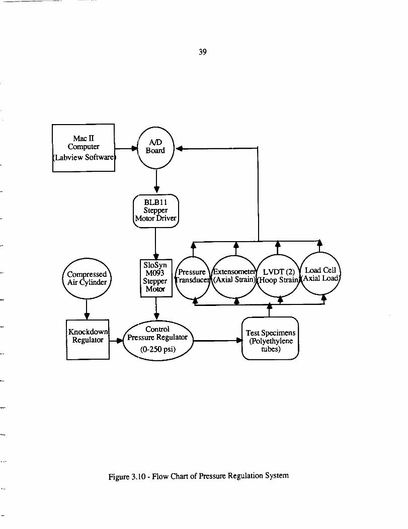
A control system designed to produced a linearly increasing air pressure was developed

during this study. The system is shown schematically in Figure 3.10, and a photograph of the

assembled system is shown in Figure 11. The pressure regulation system involved two pressure

regulators mounted in series. First, a Victor mode SR4G regulator was mounted directly on the

stem of a compressed air bottle, and reduced the nominal air pressure from 3000 psi to 300 psi.

This was referred to as the "knockdown" regulator. Air flow was then directed to a Watts R11-

03D regulator. This second regulator was referred to as the "control" regulator. The control

regulator outlet pressure can be adjusted from 0 to 250 psi. An angular rotation of the valve stem

of the control regulator results in a pressure change at the outlet. The measured outlet pressure was

found to be linearly proportional to the angular position of the valve stem. Thus, by rotating the

valve stem at a constant angular rate the outlet pressure was increased at a constant linear rate.

The control regulator was coupled to a Slo-Syn M093-FD14 stepper motor. This motor

was controlled by an Anaheim Automation BLB driver, which was in turn regulated by analog

36

voltagepulsesfrom mlA/D boardmountedin a Macintosh II computer. A single pulse from the

computer caused the ,;tepper motor shaft to turn 1.8 °. A pulse train of a given frequency would

therefore cause the motor shaft to turn at a given angular frequency. Since the shaft was coupled

to a linear pressure regulator, a given pressure rate was produced. The entire system was

calibrated such that a specified pulse rate resulted in a known linear pressure rate. A computer

program was written which allows the user to produce a pulse train of a desired frequency.

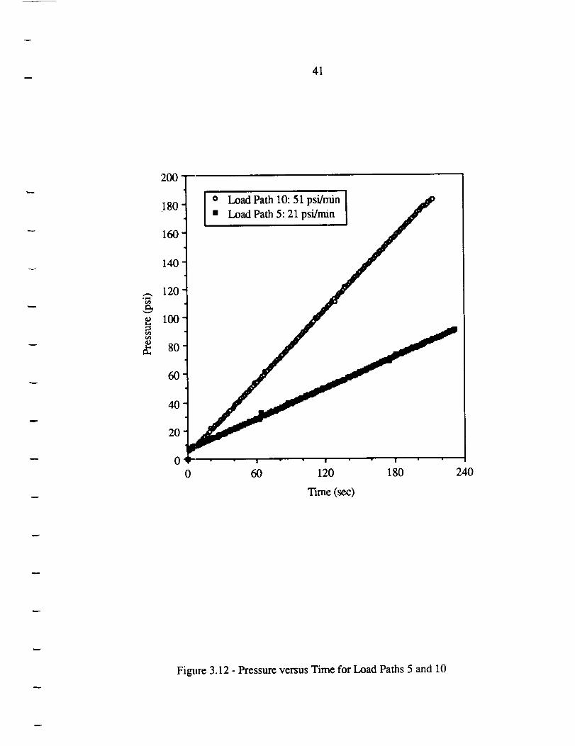
Typical plots of pressure versus time recorded along load paths 5 and 10 are shown in

Figure 3.12.

Data Acquistion

A total of five analog measurement devices were used during any test. Axial strains were

measured using an MTS model number 632.25B-20 extensometer. Hoop strains were measured

using two diametrically opposed Applied Test Systems (ATS) LVDT displacement transducers,

with a range of 0.5 inch. Pressures applied to the specimen was measured using a Gulton GS616

pressure transducer. Finally, axial loads were measured using the load cell mounted to the MTS

frame, as previously described. All five analog voltage signals were monitored using a National

Instruments NB-MIO-16H A/D board mounted within a Macintosh II computer. The A/D board

was controlled using "Labview", a National Instruments graphical programming language. The

Labview package allowed scanning rates of up to 45000 samples per second and up to 8 double-

ended input signals. One potential difficulty with the scanning process was that all 5 channels

were not monitored at the same time but rather sequentially. A maximum time lag of 5 msec

occurred between scanning each channel. Since the load and strain rates imposed during all tests

were relatively low, the 5 msec lag between measurements was negligibly small, and all 5

measurements were treated as if obtained simultaneously.

37

t Axial_

O-ring

\\

End

Clamps

PolyethyleneTube Walls

Lower

Cylinder

Air PressurePressure

Transducer

Figure 3.8 - Specimen Clamping Fixture

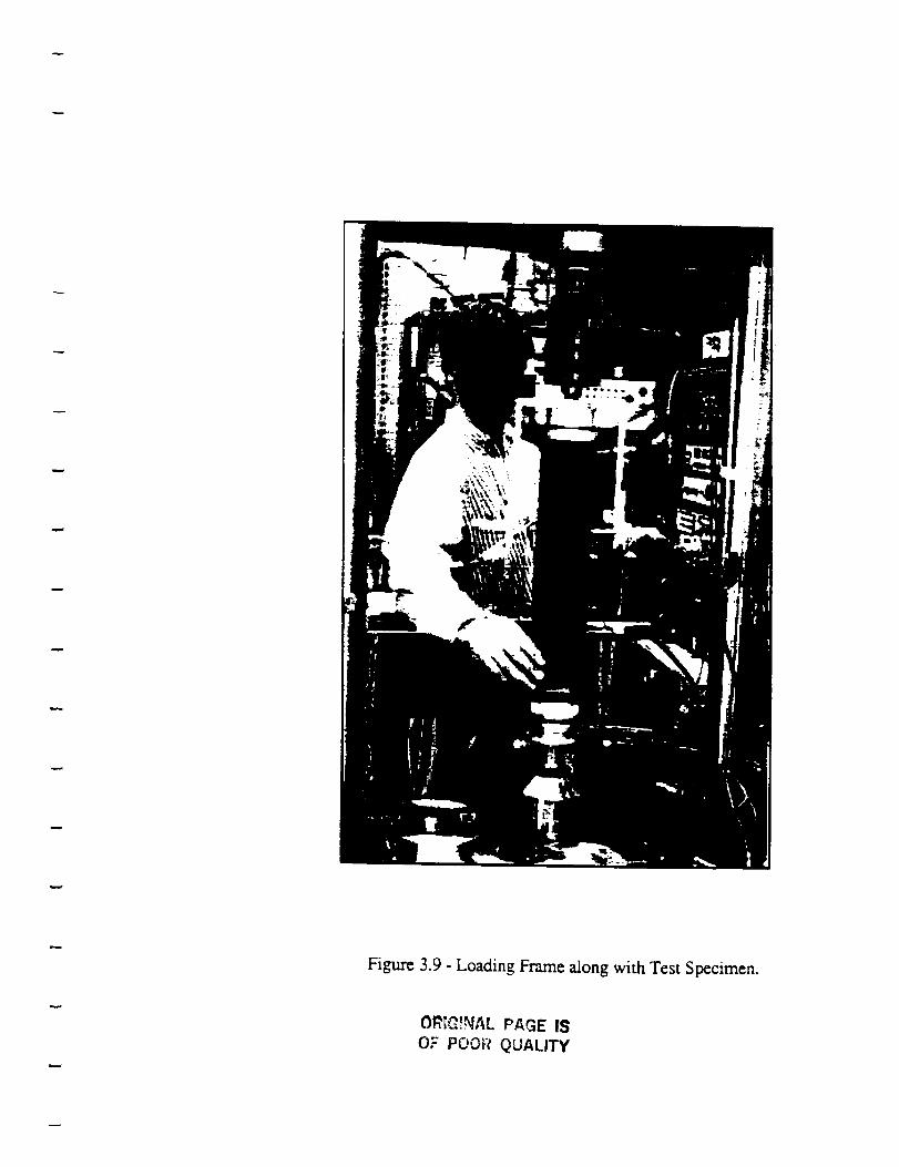
Figure 3.9 - Loading Frame along with Test Specimen.

ORIC!NAL PAGE IS

OF POOi-'tQUALITY

39

MaclI

Computer

Labview Software

Stepper /

otor Driv_

SloSynM093

StepperMotor

Regulator _ Pressure Regulator _

LVDT Load Cell

Test Specimens(Polyethylene

tubes)

Figure 3.10 - Flow Chart of Pressure Regulation System

4O

ORIGINAL PAGE IS

OF POOR QUALITY

Figure 3.11 - Pressure Regulation System

41

200

180

160

140

120

100

80

60

40

20

0

o Load Path 10:51 psi/min [• Load Path 5:21 psi/min

0 60 120 180

T'mae (sec)

240

Figlrre 3.12 - Pressure versus Time for Load Paths 5 and 10

42

The scanningprocesscreateda binarydata file. A computer program was then used to

convert the binary data to numerical voltages. A second program converted the voltage readings to

stress and strain values using calibration coefficients of the data measurement devices. Axial strain

was calculated by: (1) corLverting the voltage reading at t = 0 sec to a corresponding gage length,

(2) subtracting out the voltage reading at t = 0 sec from the entire set of voltage readings to

determine the change in voltage, and (3) multiplying the voltage readings by the calibration

coefficient 0.0992 inches/volt and dividing by the gage length for that test. Hoop strain was

calculated by: (1) subtracting the voltage reading for t = 0 sec from all voltage readings for each

LVDT, (2) multiplying the voltages for each LVDT by their corresponding calibration coefficient,

0.28457 inches/volt and 0.29379 inches/volt, to determine the displacement of each LVDT, (3)

adding the displacement for LVDT 1 at time t to the displacement of LVDT 2 at time t to determine

the total change in diameter of the tube at time t, and (4) dividing the change in diameter by the

average hoop diameter of 3.396 inches. The pressure and axial load at any time t was calculated by

multiplying the voltage reading from the pressure transducer and load cell at time t by their

respective calibration coefficients, 59.386 psi/volt and 1000 lbs/volt. The hoop and axial stresses

in the tube were calculatexl using thin-walled tube theory.

Summary of Test Procedure

Each specimen was mounted in the MTS frame, and a small offset preload (50 lbs) was

applied to allow the grips to set. The axial load was then rezeroed. The desired axial load rate was

entered into the MTS controller and all of the measurement devices and pressure hoses were

a_ched.

43

Next,anoffset pressure of approximately 7 psi was applied. The Labview program would

then begin the pressure ramp and data acquisition and the MTS axial load ramp would be started

manually. Although a small time offset existed between the start of the two ramps, the error

induced was small. An X-Y chart recorder was used to obtain an axial load versus axial strain

hardcopy plot, allowing for real-time monitoring of events. The test would end when the MTS

bottomed out, when the maximum pressure of the system was reached, or when the specimen

failed.

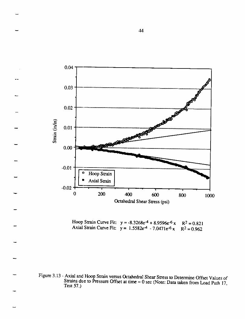
As mentioned, an offset pressure of approximately 7 psi existed in the specimen at the start

of the test. This pressure induced small strains and stresses in both the hoop and axial directions.

These strains were accounted for by plotting the hoop and axial strains versus the octahedral shear

stress, as shown in Figure 3.13. The strain values went through zero since the instrumentation

had been zeroed prior to the start of the test. The octahedral shear stress did not go through zero

since there was initially pressure in the system inducing hoop and axial stresses. The two curves

were linearly fit. An off,;et strain at time equal zero was then added to all strain values, shifting

the entire curve so that it passed through the origin. Appendix A contains plots of the experimental

hoop and axial stresses and strains obtained for each load path.

44

0.04

0.03

o_

0.02

0.01

0.00

-0.01

-0.02

o Hoop Swain [

Io Axial Strain

0 200 400 600

Octahedml Shear Stress (psi)

800 1000

Hoop Strain Curve Fit: y = -8.3268e -4 + 8.9596e-6 x R 2 = 0.821

Axial Strain Curve Fit: y = 1.5582e -4 - 7.047 le -6 x R 2 = 0.962

Figure 3.13 - Axial and Hoop Strain versus Octahedral Shear Stress to Determine Offset Values of

Strains due to Pressure Offset at time = 0 sec (Note: Data taken from Load Path 17,Test 57.)

CHAFFER 4 - DATA REDUCTION METHODS

Determination of Material Properties

Recall that load paths 1 and 19 (see Figure 3.1) define uniaxial stress tests, in which "pure"

axial and hoop stress, respectively, were applied. Four repeated tests were completed for these

two load paths. The stress and strain values recorded during these tests were used to determine

Young's modulus E and Poisson ratio v, in both the hoop and axial directions.

The experimentally determined material properties were:

E1 = 83,493 psi

E2 = 108,540 psi

v12 = 0.39

v21 = 0.52

As previously noted, the, subscript "1" has been used to denote the axial direction, while the

subscript "2" is used to denote the hoop direction. Previously reported values for E and v range

from 60,000 psi to 180,000 psi and 0.31 to 0.6, respectively [Manufacturing Chemists

Association, 1957; Rockiguez, 1982; Ward, 1975]. Measurements obtained during this study

therefore fall within the range of previously reported measurements.

The measured properties show that the annealed high-density polyethylene tubes were

anisotropic. It can be shown that these properties should satisfy the following inverse relationship

[Jones, 1975]:

46

V12 V21E1 - E2 (4.1)

Using the values of El, E2, and v12 listed above, the expected values of v21 is 0.51. This

compares very Well with the experimental value of 0.52. For consistency, the value of v21 in

subsequent calculations was forced to fit the inverse relationship, i.e., v21 was equated to 0.51.

Recall that the tubular specimens were produced by an extrusion process which resulted in

significant residual stresses in the as-received tubes. It is likely that the extrusion process also

caused the pronounced anisotropy in mechanical properties. The specimens were all subjected to a

thermal annealing treatment prior to testing, so as to relieve the residual stresses. It had been

hoped that the anneali_ag process would also reduce or eliminate any anisotropic material behavior.

This result was not achieved. The annealing process minimized residual stresses, but had little

impact upon the anisotropy of the material.

Prediction of Yielding - Isotropic Model

Although the _:est material was clearly anisotropic, it was first modeled as an isotropic

material. This approach may be of practical interest, since it avoids the additional mathematical

complexities associatezl with anisotropic constituitive models. Average values were assigned to E

and v, 96000 psi and 0.46 respectively, and were assumed constant throughout the material.

Yield was based upon a 0.3% strain offset on the octahedral shear stress- octahedral shear

strain curve. Octahedral shear stress and strain were used rather than individual axial and hoop

stress and strain components in order to determine one value for the yield point and to bypass the

47

needto averagevaluesfoundon theindividual stress-straincurves.This approachis in contrastto

themethodusedbypreviousresearchers[Raghavaet al, 1973;Ely, 1968]whereinyield is defined

basedonaxial stressandhoopstressversuseffectivestraincurves.This latterapproachresultsin

two measurementsof yield strength, which are subsequently averaged. A 0.3% offset was used

because it was the most common offset in previous yield studies on polymers [Raghava and

Caddell, 1974; Raghava et al, 1973].

The octahedral shear stress was calculated using Equation 2.2, repeated here for

convenience:

"_oct =1 (_Ol-q:_2) 2 + (02-03) 2 + (03-01) 2 (4.2)

Octahedral shear strain is a similar function of the three principal strains:

2 2+"/oct = _ ('_l-E2) (e2-C3) 2 + (e3-£1) 2 (4.3)

Since no measurement of e3 was made during testing, it was necessary to determine e3 as a

function of el and e2. Assuming that a plane stress state existed in the thin-walled tube, e3 is

related to the two measm'ed strains in the following manner:

-V

£3 = _ [£1+£2.1 (4.4)

Octahedral shear swain ,:an now be written:

48

2 '_/(2+-'_--2_T4)(812+E22) + 2ele2)'oct = 3 N (1-_)-

-v2+4v-1

(l-v) 2(4.5)

It can be shown [Semeliss, 1990] that the slope of the octahedral shear stress vs octahedral shear

strain curve, assuming isow3pic material behavior, is given by:

dx E

d"{- 2(v+l)

= G (4.6)

That is, the slope of the curve is independent of load rates and is simply equal to the shear modulus

G. This simple relationship does not hold for anisotropic material behavior, as will be shown in a

following section.

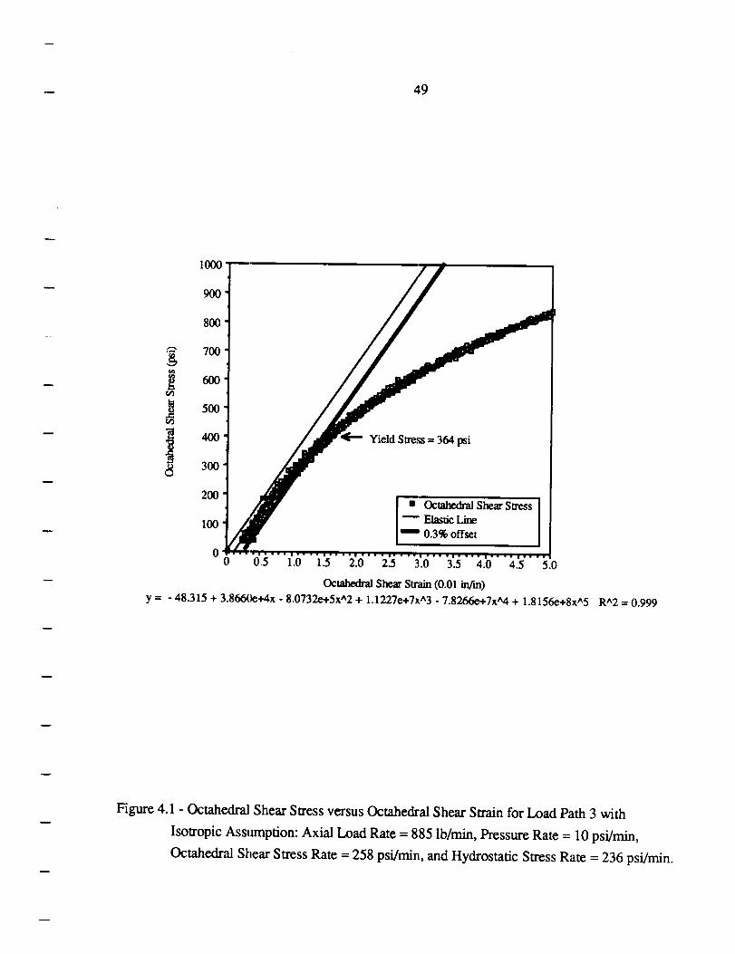
The procedure usexl to identify the yield point was as follows. Three repeated tests were

conducted along each load path. All measurements for a given load path were combined into a

single data set, and a fifth-order polynomial was fit to the data. The yield point was then identified

by calculating the point of !tntersection between a 0.3% strain offset with a slope equal to G and the

fifth-order polynomial. A typical result is shown in Figure 4.1. This numerical approach

eliminated any need for estimating the intersection visually, and defined the yield point

conveniently and consistently from one load path to the next. Since the axial stress to hoop stress

ratio was constant for each test, the axial and hoop stresses which correspond to the yield point

could be calculated based upon the octahedral shear stress at yield. Appendix B contains plots of

octahedral shear stress versus octahedral shear strain for all load paths.

49

1000

900

800

700

6oo

500

i °8 300

Yield Stress = 364 psi

2OO

.__i Octahedral Shear Stress100 Elastic Line

0.3% offset

00 0.5 1.0 1.5 2.0 2.5 3.0 3.5 4.0 4.5 5.0

Ck-,tahedral Shear Strain (0.01 in/m)

y = - 48.315 + 3.8660e+4x - 8.0732e+5x^2 + 1.1227e+7x^3.7.8266e+7x_4 + 1.8156e+8x^5 R^2 = 0.999

Figure 4.1 - Octahedral Shear Stress versus Octahedral Shear Swain for Load Path 3 with

Isotropic Assmnption: Axial Load Rate = 885 lb/min, Pressure Rate = 10 psi/min,

Octahedral Shear Stress Rate = 258 psi/min, and Hydrostatic Stress Rate = 236 psi/min.

50

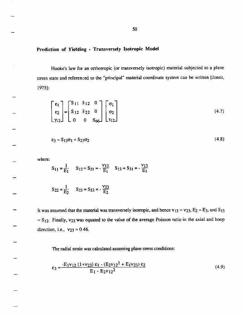
Prediction of Yielding - Transversely Isotropic Model

Hooke's law for an orthotropic (or transversely isotropic) material subjected to a plane

stress state and referenced to the "principal" material coordinate system can be written [Jones,

1975]:

el FSll , 12 0 _1

C2 = 2 S 22 a2

TI2 0 Xl

(4.7)

E3 = Sl3t_l + $23ff2 (4.8)

where:

I v12 V13SII =Eli S12 = $21 = - _1 S13 = S31 = - E--I-

V23$22 = E_ $23 = $32 = - E"-2"

It was assumed that the material was transversely isotropic, and hence v13 = V23, E2 = E3, and S13

= S12. Finally, v23 wa:_ equated to the value of the average Poisson ratio in the axial and hoop

direction, i.e., v23 = 0 46.

The radial strain was calculated assuming plane stress conditions:

e3 - -EIV12 (1 _-v23) el - (E2v122 + E1v23) e2 (4.9)E 1 - E2v 122

51

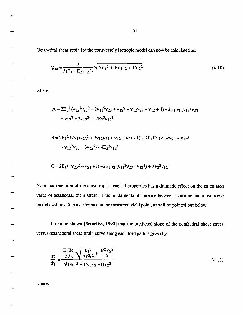
Octahedralshearstrainfor the transversely isotropic model can now be calculated as:

----_/Ael 2 + Bell_2 + C1_22 (4.10)Toct- 3(El - E2Vl2 z)

where:

A = 2El 2 (V122V232 + 2V122V23 + V122 + V12V23 + V12 + 1) - 2ElE2 (v123v23

+ V123 + 2V122) + 2EE2V124

B = 2El 2 (2v12v232 + 3v12v23 + v12 + v23 - 1) + 2E1E2 (v123v23 + v123

- v122v23 4. 3v122) - 4E22v124

C = 2El 2 (v232 _- v23 +1) +2E1E2 (v122v23 - v122) + 2E22v124

Note that retention of the anisotropic material properties has a dramatic effect on the calculated

value of octahedral shear strain. This fundamental difference between isotropic and anisotropic

models will result in a difference in the measured yield point, as will be pointed out below.

It can be shown [Semeliss, 1990] that the predicted slope of the octahedral shear stress

versus octahederal shear strain curve along each load path is given by:

_/ 3r2k22E1E2 kl 2 +

dx 2"_ 2_2r 2 2

d_/ Nff_l 2 + Fklk2 +Gk22(4.1 1)

where:

52

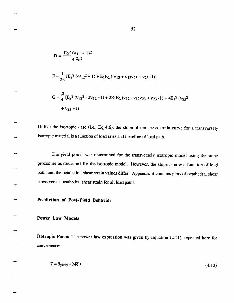
D -- E22 (V12 + 1)2

4r2r; 2

1 [E22 (_Y122 + 1) + E1E 2 (-v12 + v12v23 + v23 -1)]F=2/t

r 2G = _- [-E22 (vi,22 - 2v12 +1) + 2E1E2 (v12 - v12v23 + v23 -1) + 4E12 (V232

+ V23 +1)l

Unlike the isotropic case (i.e., Eq 4.6), the slope of the stress-strain curve for a transversely

isotropic material is a tunction of load rates and therefore of load path.

The yield point was determined for the transversely isotropic model using the same

procedure as described for the isotropic model. However, the slope is now a function of load

path, and the octahedr_d shear strain values differ. Appendix B contains plots of octahedral shear

stress versus octahedral shear strain for all load paths.

Prediction of Post-Yield Behavior

Power Law Models

lsotropic Form: The power law expression was given by Equation (2.1 1), repeated here for

convenience:

s = Syield + MEn (4.12)

53

where:

11

=_[(Sl_S2)2+ (s2_s3)2+ (s3_sl)2 ] 2

(4.13)

1

= _ [(el -e2)2 + (e2-e3) 2 + (e3-el)212(4.14)

are the effective true stres:_ and effective true strain defined as a function of the principal stresses

and strains respectively. Assuming plane stress, then s3 = 0, and Equation (4.13) can be

simplified:

1

= [s12 + s2 2 + SlS2] _ (4.15)

Also by assuming the constancy of volume, Equation (4.14) can be rewritten as:

14 - (4.16)

= [3 (el2 + e22 _"ele2)]2

The true strains used in Equation (4.16) are the plastic portion of the total true strain defined earlier

and repeated here:

ep = et_ ee(4.17)

where e t and ee are the total and elastic true strain components respectively. The total true strain e t

are the experimentally recorded values and the elastic true strains ee are defined using the biaxial

54

form of Hooke'slaw. ']'he principal stress and strain components in Equations (4.15) and (4.16)

correspond to the axial and hoop directions, due to loading and specimen geometry symmetry.

Taking the logarithms of both sides of Equation (4.12) gives:

log(-g-_yield) = n IogE + logM (4.18)

which is in the form of a linear equation:

y -- mx + b (4.19)

where y -- log s-syield, x = logE and b = logM. Thus, a log-log plot of S-syield versus E- can be

used to determine the constants M and n, where M is the y-intercept and n is the slope of Equation

(4.19).

A polynomial curve-fit was used to achieve a smooth curve after shifting the individual

tests to the isotropic yieht points. A "new" data set consisting of axial stress strain and hoop stress

strain values was generated using the polynomial curve-fitting equation. The effective true stresses

and effective plastic strains were then calculated using Equations (4.15) and (4.16). A log-log plot

of s-s-yield versus _ was performed and a linear curve-fit was used to achieve the best correlation

coefficient. This linear curve-fitting equation provided easy calculation of the constants M and n,

the strength coefficient and strain hardening exponent, respectively.

Anisotropie Form: For the anisotropic case, the power law relation is defined in the same way

as the isotropic case given by Equation (4.12). On the other hand, the effective true stress and

55

effectivetruestrainfor ananisotropicmaterialunder complex loading condtions are very different

from the isotropic case (compare Equations 2.12 and 2.13 with Equations 2.23 and 2.24).

However, if it is assumed that only a biaxial stress state exists and the material is transversely

isotropic, then Equations (2.23) and (2.24) can be simplified as:

._.

(4.20)

_/_F+G+H)[F {Ge2 +H(el+e2)}2" G {FeI+H(el+e2) }2 + H{Fel-Ge2} 2]

E = -----_HF

(4.21)

where:

1

H+G=_

1

H + F = T2hoop

H=G

The coefficientS, F, G, _tad H, are now functions of the tensile yield strengths in the axial and

hoop directions.

Using Equations (4.12), (4.20) and (4.21), the constants M and n can again be found

using a linear curve-fit of a log S-Syield versus log _ curve.

56

PrandtI-Reuss Model

The Prandtl-Reuss equation for an

repeated here for convenience:

isotropic material was given in Equation (2.20),

3 s] d_ ds_ (1-2v)

de_ - 2 s-H _ + _ dShyd (4.22)

where _ is the isotropic form of the effective true stress defined by Equation (4.15). Equation

(4.22) gives the increraental change in total true strain associated with an incremental increase in

stress. Note that by definition the plastic true strains equal zero at the yield point. Therefore the

total true swain induced by a given stress state beyond the yield point equals the sum of the elastic

response (including any strain offset associated with the definition of yielding) plus the sum of

incremental increases, in strain calculated using Equation (4.22). The given stress state is

represented by the effective true stress g, the deviatoric stress, and the hydrostatic true stress

Shyd.

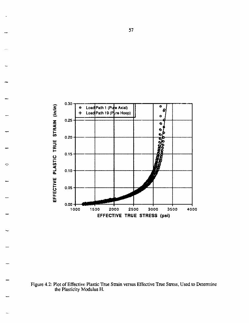
In order to apply the Prandtl-Reuss equation in practice, one must determine the material

constants E and v, as well as the plasticity modulus H. In the present case E and v were assigned

average values of 96(N30 psi and 0.46. The plasticity modulus H was determined using data

collected along the two uniaxial stress load paths, specifically load path 1 (pure axial stress) and

load path 19 (pure hoop stress). Four repeated tests were performed along both of these load

paths. The resulting eight data files were combined into a single data set and a plot of effective

plastic true strain versus effective true stress was generated, as shown in Figure 4.2. The data was

57

0.00 -

1000 1500 2000 2500 3000 3500 4000

EFFECTIVE TRUE STRESS (psi)

Figure 4.2: Plot of Effective Plastic True Strain versus Effective True Stress, Used to Determinethe Plasticity Modulus H.

58

thencurve-fitusingafifth-orderpolynomialsuchthatthederivativeof thisequationrepresentsthe

inverseof theplasticitymodulusH:

1 d_-p(4.23)

As mentioned above and described in a preceding section, yielding was detrmed in terms of

a 3% offset in octahedral shear strain, and the axial and hoop strain components associated with

this strain offset were added to the calculated elastic strains.

Lode Parameters: The Lode parameters, I.t and v, provide a simple check to determine if the

Prandtl-Reuss equations are valid for a given material. If the equations hold, then g and v are

equal, as previously shown in Figure 2.2. For plane stress conditions the Lode parameters reduce

to:

= 2s2- SlSl

V m

where in the present case the principal stresses and strains correspond to the axial and hoop

directions. The stresses in Equation (4.26) are the total stresses, while the plastic strains were

derived also from experimental values using Equation (4.17). The parameters la. and v were

calculated for the the entire post-yield history, and then an average value was determined for each

particular load path.

CHAPTER 5 - RESULTS AND DISCUSSION

YIELD PREDICTIONS

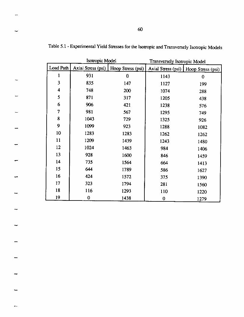
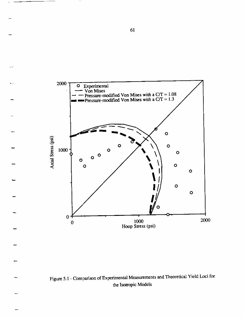
Isotropic Models: The two isotropic yield criterion considered in this study were the Von Mises

yield criterion and the Pressure-modified Von Mises yield criterion. Experimentally determined

yield points are listed in Table 5.1, and are compared with predictions in Figure 5.1 Note that the

shape and size of the theoretical Pressure-modified Von Mises locus is a function of the

compressive to tensile yield strength ratio (see Eq 2.4). Since the compressive yield strength of

polyethylene was not measured during this study, it was neccessary to use literature reference

values for the compressive to tensile yield strength ratio (C/T) for high-density polyethylene. Two

values have been reported in the literature for (C4T): 1.3 [Raghava and Caddell, 1973] and 1.08

[Raghava et al, 1973; Caddell et al, 1974]. Thus, the compressive yield strength is typically higher

than the tensile yield strength.

The comparison presented in Figure 5.1 shows that the experimental measurements were

not well predicted by either of the two isotropic yield criterion considered. The theoretical loci

were symmetric with respect to the 45 ° line, while the experimental yield locus was skewed. This

discrepancy is of course due to material anisotropy. As previously stated, the isotropic analysis

was conducted because isotropic models avoid the additional mathematical complexities associated

with anisotropic consti_uitive models, and hence are easier to apply in practice. The results

represented by Figure 5.1 show that very significant errors are introduced by the assumption of

isotropy.

60

Table5.1- ExperimentalYield Stressesfor theIsotropicandTransverselyIsotropicModels

IsotropicModelLoad Path

1

3

4

5

6

7

8

9

10

11

12

13

14

15

16

17

18

19

Axiat Stress (psi) Hoop Stress (psi)

931 0

835 147

748 200

871 317

906 421

981 567

1043 729

1099 923

1283 1283

1209 1439

1024 1463

928 1600

735 1564

644 1789

424 1572

323 1794

116 1293

0 1438

Transversely Isol_ Dpic Model

Axial Stress (psi) [ Hoop Stress (psi)

1143 0

1127 199

1074 288

1205 438

1238 576

1295 749

1325 926

1288 1082

1262 1262

1243 1480

984 1406

846 1459

664 1413

586 1627

375 1390

281 1560

110 1220

0 1279

61

20000 Experimental

VonMises-- --- Pressure-modifiedVonMiseswith aC/T = 1.08_. m Pressure-modified Von Mises with a C/T = 1.3

&

o'1

_4<

1000

o

o

OO

o °

!

o

o

o

0

o

0

0

0

0

0 1000 2000

Hoop Stress (psi)

Figure 5.1 - Comparison of Experimental Measurements and Theoretical Yield Loci for

the Isotropic Models

62

2O00

C, ExperimentalB_ Tsai-HiU

-- Pressure-modified Tsal-HiU with a Cfl" = 1.08_" '_Pressure-modified Tsai-Hill with a _T = 1.3

&

<

1000'

o \o _ a

o

o

o

0

0 1000 2000

Hoop Stress (psi)

Figure 5.2 - Comparison of Experimental Measurements and Theoretical Yield Loci for

the Transversely Isotropic Model

( t I ! I ! I , ,

Standard Deviation

........ J

//

0

t_

64

It was concluded on the basis of these results that the yield behavior of high-density

polyethylene cannot be adequately modeled using isotropic yield criterion. Further, this conclusion

is likely to be true for the general class of semi-crystalline thermoplastic polymers.

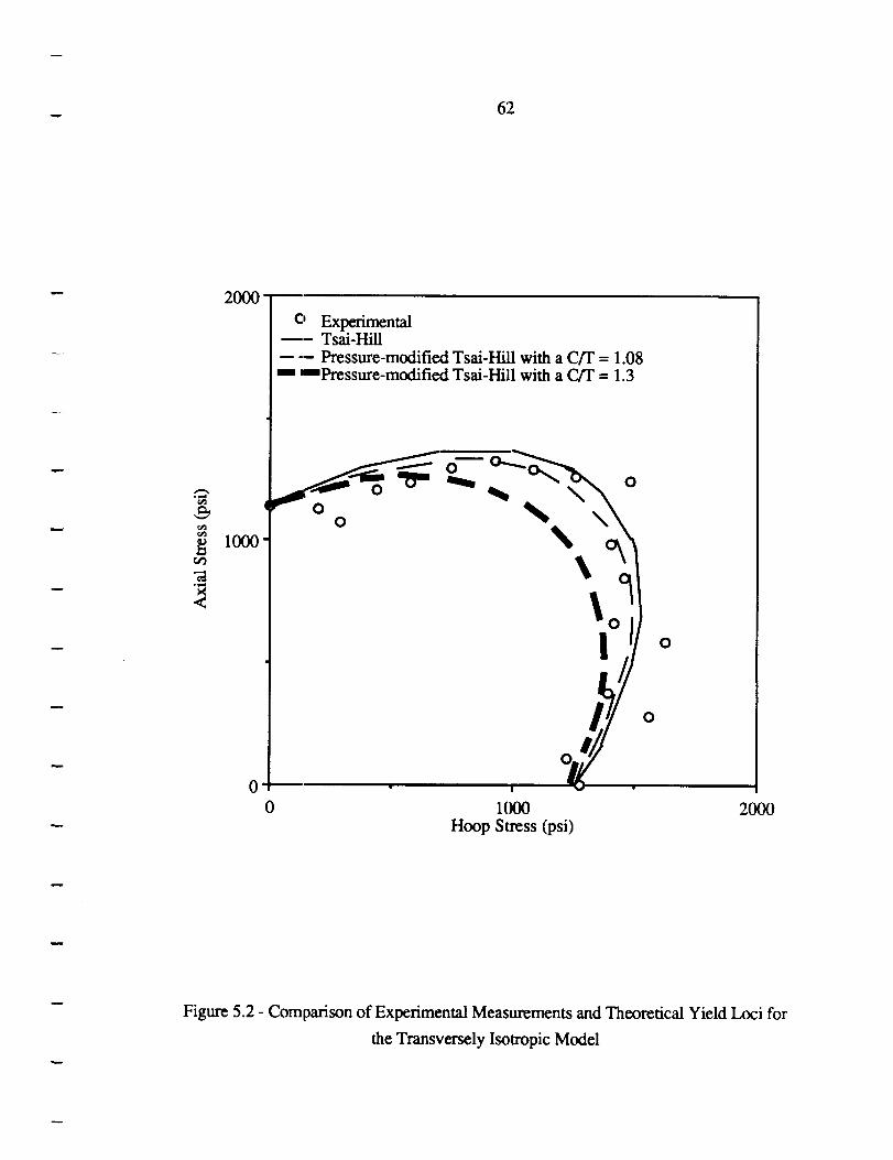
Anisotropic Models: The two anisotropic yield criterion considered in this study were the Tsai-

Hill criterion and the Pressure-modified Tsai-HiU criterion. Experimentally measured yield points

based on the transversely isotropic model are listed in Table 5.1. A comparison of the

experimental yield locus and the predicted loci of the two anisotropic models is shown in Figure

5.2. Once again, the compressive to tensile yield strength ratio was needed to define the theoretical

Pressure-modified Tsai-hIill yield locus (see Eq 2.6). In this case both hoop and axial strength

ratios are required. The same values for the strength ratios mentioned above were used (i.e., C/T

= 1.3, 1.08), and the ratios were assumed to be the same for both hoop and axial directions.

Comparing Figs 5.1 and 5.2, it is immediately obvious that the anisotropic models predict

the experimental behavior much better than the isotropic models. However, by inspection alone it

is difficult to determine whether the Pressure-modified Tsai-Hill yield criterion or the Tsai-Hill

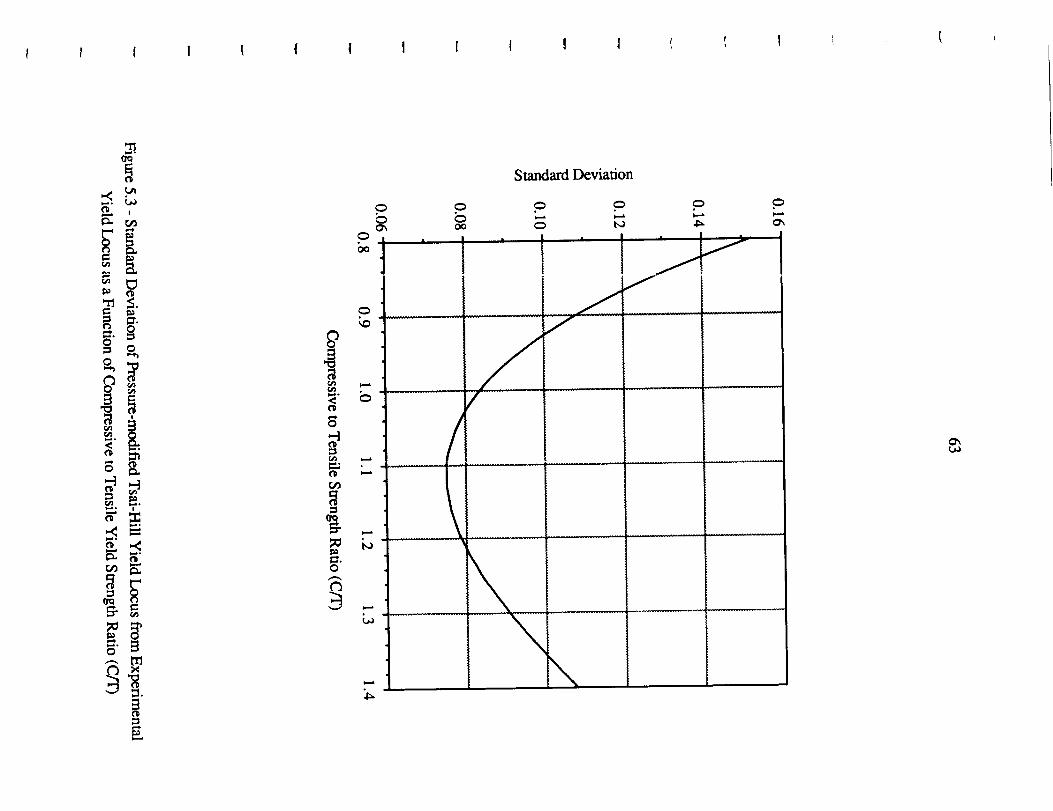
yield criterion best fit the experimental results. A calculation based on the standard deviation

between measurement and prediction was conducted to determine which criterion correlated best

with experimental results. The procedure is fully described in Appendix C. Briefly, the standard

deviation was based on the difference between the radial distance to an experimentally measured

yield point and the radial distance to the corresponding point on the theoretical yield locus defined

by the Pressure-modified Tsai-Hill criterion and some given C/I" ratio. In essense, the procedure

determined the particular C/I" ratio which resulted in the best fit between measured and predicted

yield response.

65

The standarddeviationasa functionof theC/T ratio is shownin Figure 5.3. Theresults

indicateaminimumstandarddeviationwhenthestrengthratiowas1.11. As discussedabove,C/T

ratios for highdensity polyethyleneequalto 1.08and 1.3havebeenreported. Hence,the C/T

ratio deducedfrom the datacollectedduring this study is in close agreementwith previously

reportedvalues.

To summarize,theyield responseof annealedhigh-densitypolyethyleneis bestpredicted

usingthePressure-modifiedTsai-Hill criterion,with aC/T ratioof 1.11.This criterionadequately

modelsboththeanisolropicnatureof polyethylene,andalsoaccountsfor theeffectsof hydrostatic

stressonyielding.

POST-YIELD PREDICTIONS

Power Law Model

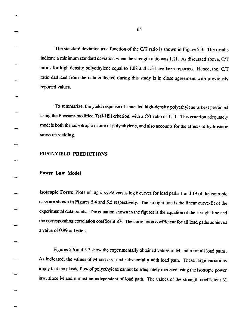
Isotropic Form: Plots of log _-_yieid versus log _ curves for load paths 1 and 19 of the isotropic

case are shown in Figa_res 5.4 and 5.5 respectively. The straight line is the linear curve-fit of the

experimental data points. The equation shown in the figures is the equation of the straight line and

the corresponding comflation coefficent R 2. The correlation coefficient for all load paths achieved

a value of 0.99 or better.

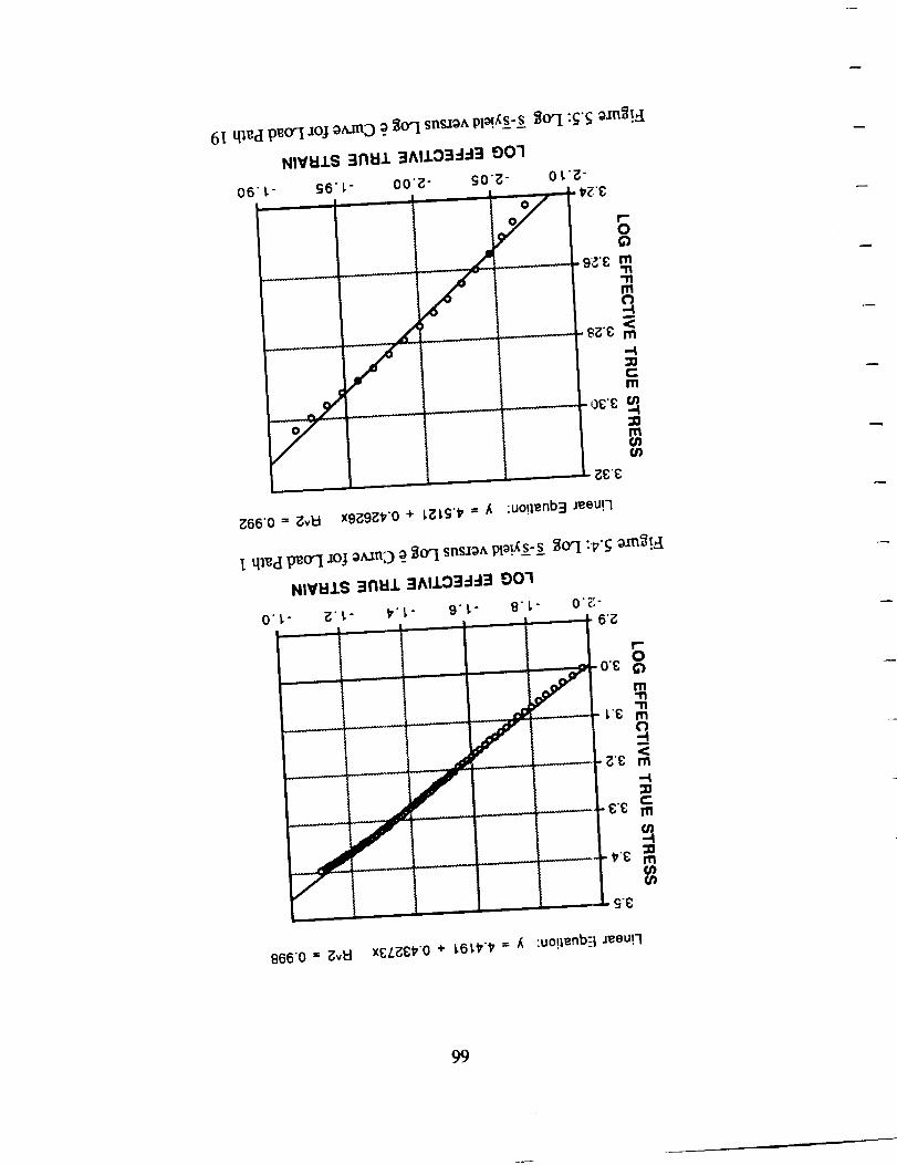
Figures 5.6 and 5.7 show the experimentally obtained values of M and n for all load paths.

As indicated, the values of M and n varied substantially with load path. These large variations

imply that the plastic flow of polyethylene cannot be adequately modeled using the isotropic power

law, since M and n must be independent of load path. The values of the strength coefficient M

61 q_¢d p¢o'I ._oj o_xnD o ilo'I sn_o^ PlO!/_S_-s_ _O"I "g'g o-tn_._ [

NIVH.LS 31')1::113AI-L C)3"1"1:_ 00"1

•_- s6" L- oo'_- so'_- o t_-

...... - _;_'£

mt_0')

;_66"0 = ;_vEI x9;_9Z¢'O + I._l.S't_ = /_ :uo!lenb=l jeeu!7

I ql_d p¢o"l .toj oMno o_i]O"l snsdo^ PlO.tgs-s- _0"I :_'_ oala_t._I

NIVHIS =113111=IAIIO =I'I'I=I 00"I

O'k g't- t_'k" 9"t" 8" O'Z:"" 6"_

I"

0"£ g

.g'g

Po"£'8 I_I

_q

866"0 = _vH x£L;_;'_'O + 1,61,t_'_'= _ :u°!_enb-I aeeu!7

99

67

50000

45000

I--Z 40000UJ

35000Iii1UJ 300000

25000-r"I-.(,:1 20000ZWn-. 15000I--(/) 1000O

5000 "

I I I I I I I I l I I I I I I l I

2 3 4 5 6 7 8 9 1011 121314 151617 1819

LOAD PATHS

Figure 5.6: Stren_gth Coefficient M versus Load Path for Isotropic Power Law Model

0.50

r-

I-ZtU 0.45ZOO.XW

0.40(.9ZZILlO 0.35re

"I"

Z0.3o

rek-

0.25 = I I I I I I I I I I I I I I I I I

2 3 4 5 6 7 8 9 101112131415161718 9

LOAD PATHS

Figure 5.7: Strain tlardening Exponent n versus Load Path for Isotropic Power Law Model

68

10000

9000I-ZLU

_o 8o001,1.1,1.I,U

0 7000t..)

-n-1-

6O00ZIMerI,- 5000

4000I I I l I I I I I I I I I I I I I

2 3 4 5 6 7 8 9 1011 12131415161718

LOAD PATHS

9

Figure 5.8: Strength Coefficient M versus Load Path for Anisotropic Power Law Model

c

f-Zi,iZ0a.xuJ

zzi,i

rr

-r-

Z

n-I-(n

0.45

0.44

0.43

0.42 • • • • • • •0.41

0.40 • •

0.39 •

0.38 • • • •

0.37

0.36

0.35 ' , , , . , , , , , , , u , , . ,

1 2 3 4 5 6 7 8 9 101112131415161718

LOAD PATHS

Figure 5.9: Strain Hardening Exponent n versus Load Path forAnisotropic Power Law Model

69

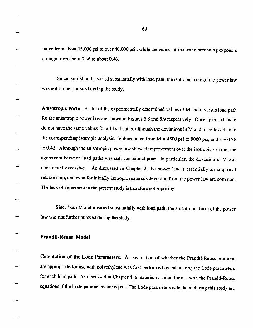
rangefrom about15,£00psi to over40,000psi, while thevaluesof thestrainhardeningexponent

nrangefrom aboutO.36to about0.46.

SincebothM andn variedsubstantiallywith loadpath,the isotropicform of thepowerlaw

wasnot furtherpursuedduring thestudy.

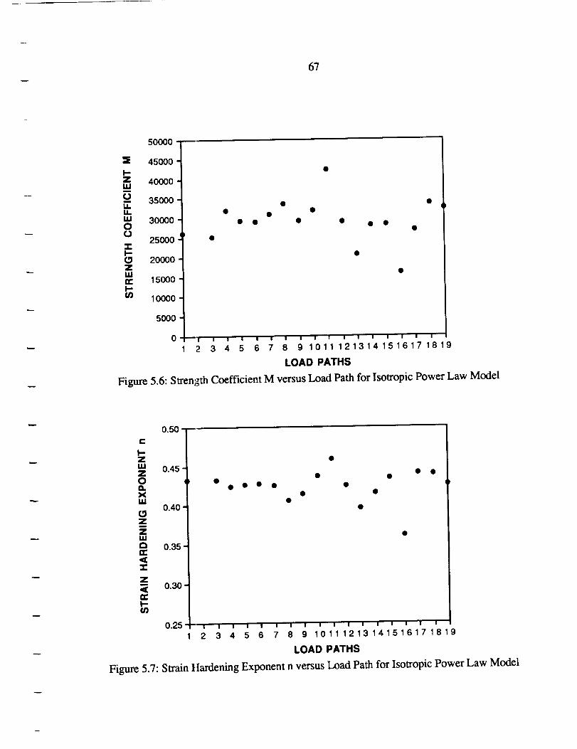
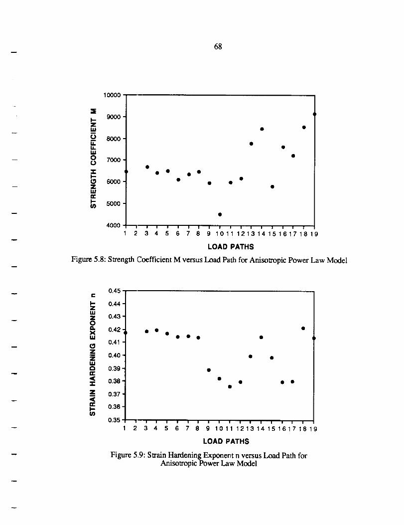
Anisotropic Form: A plot of the experimentally determined values of M and n versus load path

for the anisotropic power law are shown in Figures 5.8 and 5.9 respectively. Once again, M and n

do not have the same values for all load paths, although the deviations in M and n are less than in

the corresponding isolropic analysis. Values range from M = 4500 psi to 9000 psi, and n = 0.38

to 0.42. Although the anisotropic power law showed improvement over the isotropic version, the

agreement between load paths was still considered poor. In particular, the deviation in M was

considered excessive. As discussed in Chapter 2, the power law is essentially an empirical

relationship, and even for initially isotropic materials deviation from the power law are common.

The lack of agreement in the present study is therefore not suprising.

Since both M and n varied substantially with load path, the anisotropic form of the power

law was not further pursued during the study.

Prandtl-Reuss Model

Calculation of the Lode Parameters: An evaluation of whether the Prandtl-Reuss relations

are appropriate for use with polyethylene was f'trst performed by calculating the Lode parameters

for each load path. As discussed in Chapter 4, a material is suited for use with the Prandtl-Reuss

equations if the Lode parameters are equal. The Lode parameters calculated during this study are

I

70

shown in Figure 5.10. Although the parameters were not absolutely identical, the deviations are

similar in magnitude to those reported by other researchers for other materials (see, for example,

Figure 2.2). Hence, the Lode parameters indicate that the Prandtl-ReusS relatiOnS will predict the

post-yield response to within engineering accuracy, which in essence implies that high-denSity

polyethylene can be modeled approximately as an dasfic-perfectly plastic material.

Figures 5.11- 5.28 show a comparison between experimental

PrandtI-ReuSS predictiOnS: hoop strain for each load path, based upon the Prandtl-Reuss

and predicted axial strain aad

equatiOnS. The reader shou'td note several details during interpetati°n of these plots. First, the

stress and strains plotted in these figures are true stress/strainS, as compared to engineeringpost-yield response is plotted. As previOUSly discussed, allthe

stress/strainS- Second, only the

curves (both measured and predicted) begin at the axial or hoop strain level associated with

yield point for the given load path. These strain levels were calculated as the sum of the elastic

strain at yield (calculate_l using the average measured values of E and v), and a strain value

corresponding to the 0.3% offset in octahedral shear strain. Third, strains are plotted against both

axial and hoop stress in t_ese figures, to emphasize that the measured and predicted response is for

a particular biaxial loading condition. Fourth, the maximum plastic strain which could be induced

was not constant for all load pathS. Recall that axial loads were applied using an MTS fatigue

capable of applying loads as high as 20,000 lbs. In contrast, internal pressures were applied

frame and regulator system, and the maximum pressure which could be applied was• "ch could be induced for a gaven load path

using a bottled air "n wm "• . -imum plastic strat • -- loading mechanism-

roughly 250 psi. Hence, the max _ _ _ :_,o,_,! rxessure was the dotrnnam

was a function of whether the axial loatl or _,,,. ..... "

in order to make a consistent comparison, the strain range for Figs 5.11 through 5.18 (i.e., for

load paths 1 through 9) is 0 to 0.20 in/in, whereas the strain range for Figs 5.19 through 5.28

_ 0oad paths 10 through 19) is 0 to 0.10 in/in. Fifth, in each plot the predicted response is

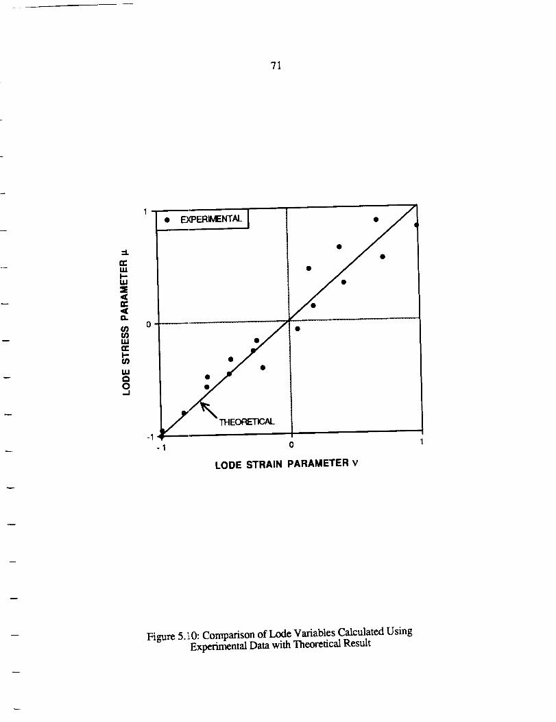
71

I • F_XPERIMENTN- I

=L

o

-I

-I

• q

LODE STRAIN PARAMETER v

Figure 5.!0: Comparison of Lode Variables Calculated UsingExperimental Data with Theoretical Result

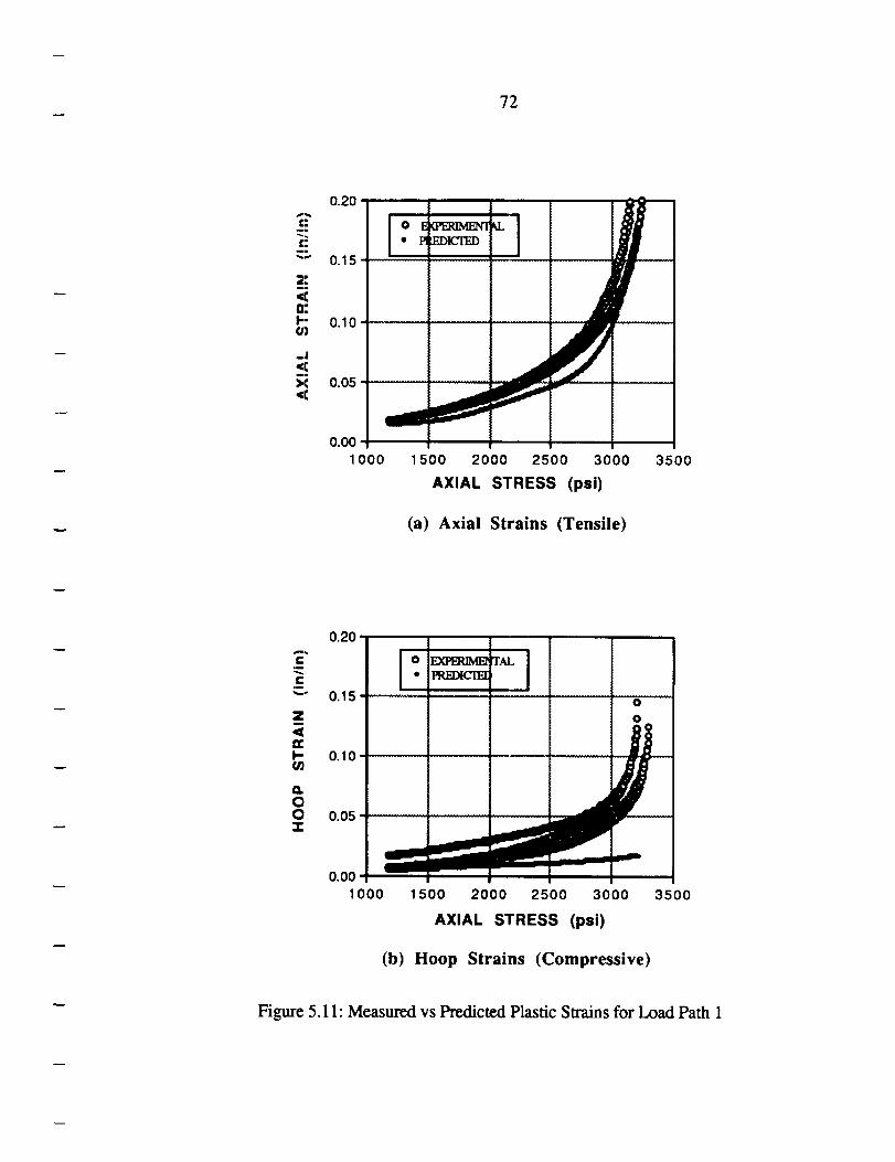
72

£-.o..

t:

nm

<a:I--oi

_.1<

<

0.20

0.15

0.10

0.05

• PI',/_ICTED IH#

0.00

1000 1500 2000 2500 3000

AXIAL STRESS (psi)

3500

(a) Axial Strains (Tensile)

.__ o _ T_.

""" 0.15 ........................................................... o '

n

I-

Q.OOZ:

0.10

0.05 _

0.00'

1000 1500 2000 2500 3000 3500

AXIAL STRESS (psi)

(b) Hoop Strains (Compressive)

Figure 5.11: Measured vs Predicted Plastic Strains for Load Path 1

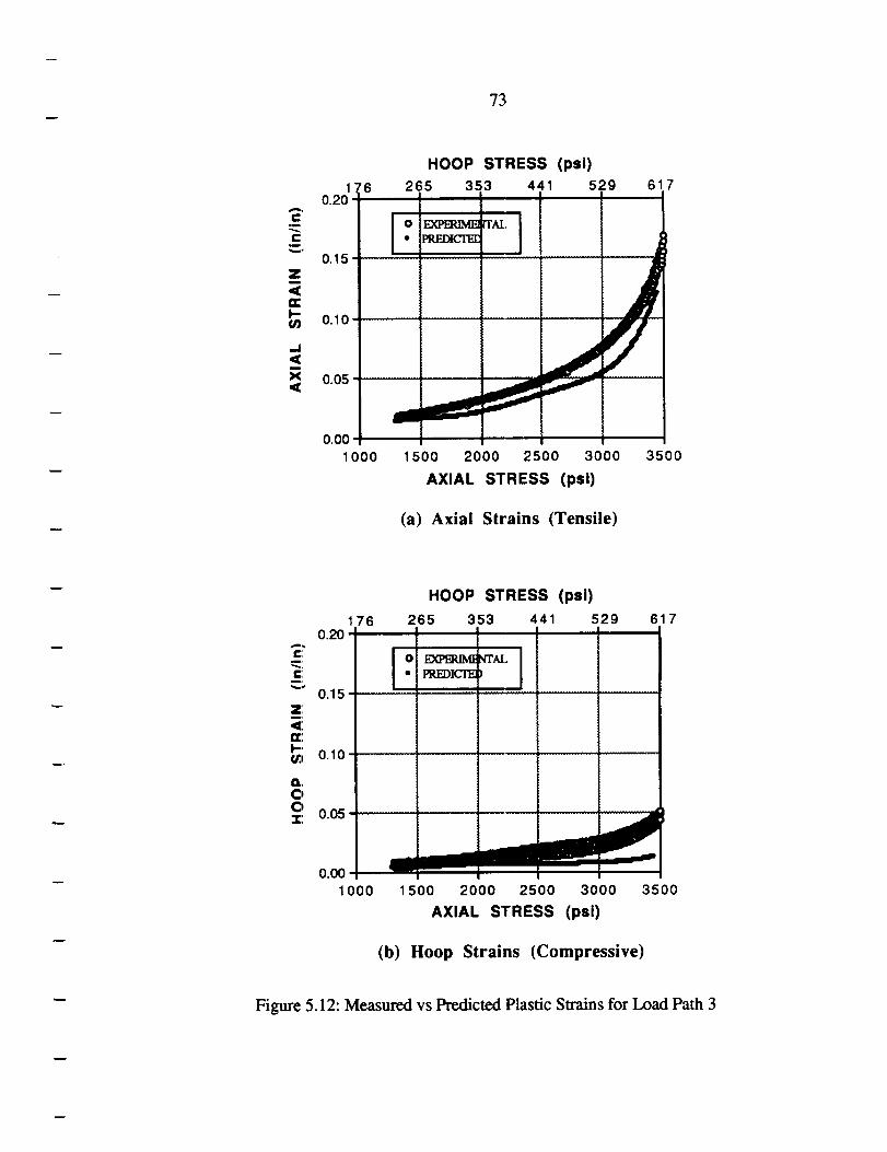
73

,m

r-

Zm

<

k-u3

<I

X<

1 '60.20

HOOP STRESS (psi)

265 353 441 529 617

0.15

0.10

0.05

J0.00

1000 1500

J

2000 2500 3000

AXIAL STRESS (psi)

35O0


e:,l,

¢:

0.1Z:m,

<:er:I--,_l 0.10

D,,Oo_: 0.05

176

0.00

1000

HOOP STRESS (psi)

265 353 441 529 617

O! EXPER_g NTAL• I_.t_ICI_

1500 2000 2500 3000 3500

AXIAL STRESS (pal)



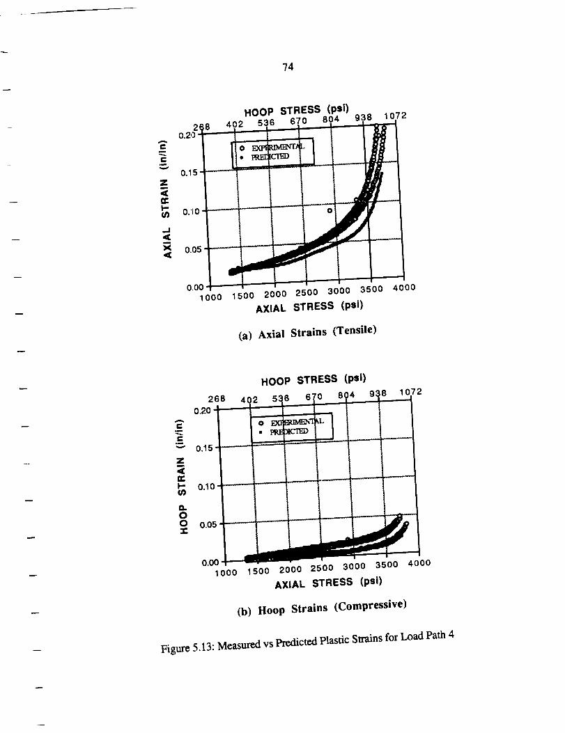
74

HOOP STRESS (psi)

Z

0,00"t-1000 1500 2000 2500 3000 3500 4000

AXIAL STRESS (psi)


e-

_-" 0.15

Z

k- 0.10O_

O.oO 0.05

HOOP STRESS (psi); 1072

268 4(_ ! 53 ; 63 ) 8( _ -...-.--

0.20 _ _

• pl_ ICTED

k_ _-_--_-

0.00"1000 1500 2000 2500 3000 3500

AXIAL STRESS (psi)

4000



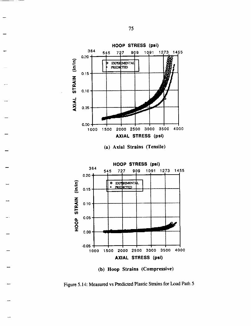
75

HOOP STRESS (psi)

364 545 727 909 1091 1273 14550.20 •

0.10 ................

0.00

1000 1500 2000 2500 3000 3500 4000

AXIAL STRESS (psi)


364

0.20 -

HOOP STRESS (psi)

545 727 909 1091 1273 1455

A

_- • .__.__ 0.15

Zi

I-

0.10 .................

0.05 ...............

o0z c.oo ---...a_lm__

-0.05

1000 1500 2000 2500 3000 3500 4000

AXIAL STRESS (psi)



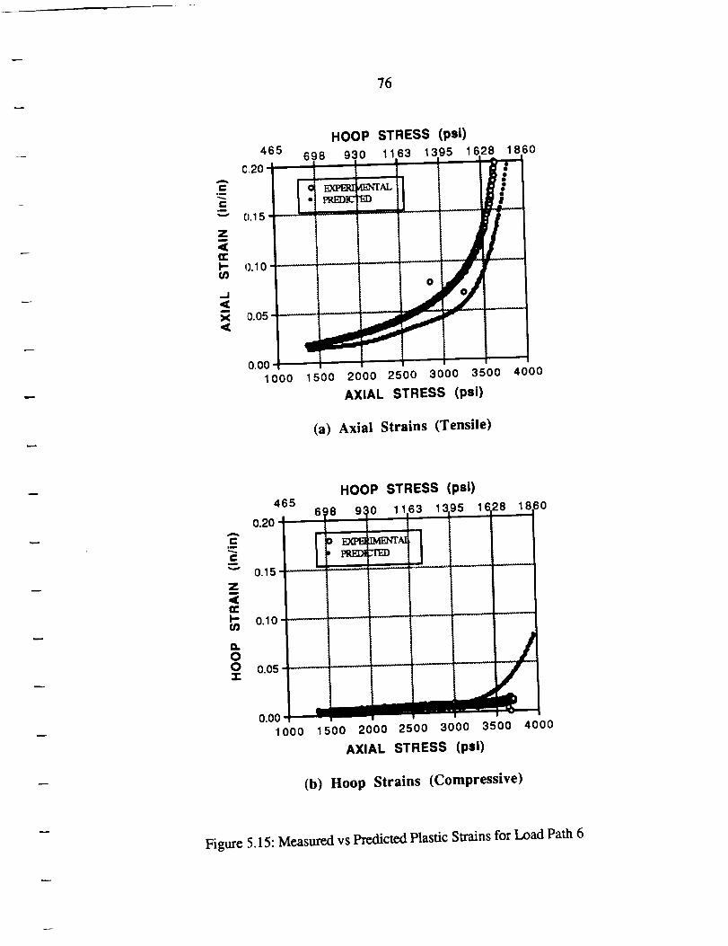
76

HOOP STRESS (psi)

465 6989301163139516281860

C,20 I_

o EXp_d]_h'TAL _ .

Z

=,,.,o........i' -/.I0.05

0.001000 1500 2000 2500 3000 3500 4000

AXIAL STRESS (psi)


465

0.20

,g

c,m

"" 0.15

Z

n-_" 0.10 -

o.OO O.O5

HOOP STRESS (psi)

/

_0

0.001000 1500 2000 2500 3000 3500 4000

AXIAL STRESS (psi)



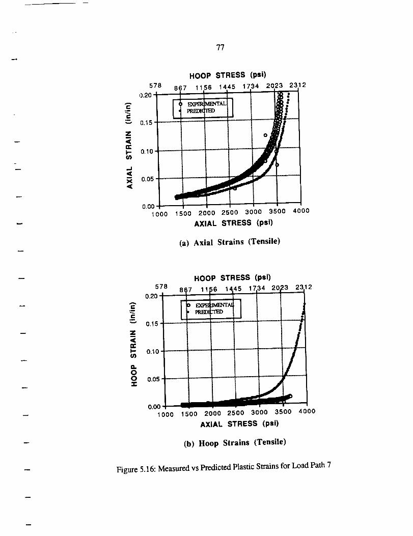
?7

HOOP STRESS (psi)

578 867 1156 1445 1734 2023 2312

_ H_EDICTED

0.15

Z

0.10 ............. F ....

0.05 "--"--- :

0.001000 1500 2000 2500 3000 3500 4000

AXIAL STRESS (psi)


HOOP STRESS (psi)578

0.20"A

e. o EXT_ n_TAI

•_ m Ht_D] _ED /"" 0.15 .............................

<

k- 0.10 ....(n

a.OO o.o5q-

0.001000 1500 2000 2500 3000 3500 4000

AXIAL STRESS (psi)

(b) Hoop Strains (Tensile)


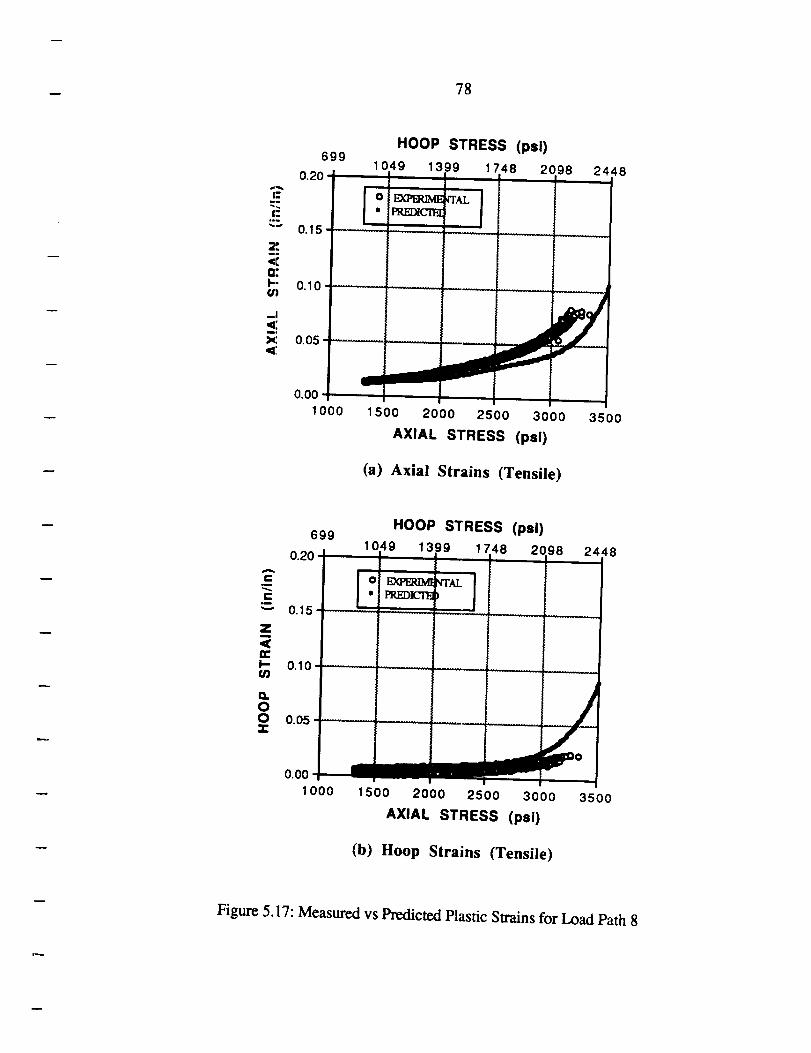
78

r.

i.=,=l

Zii

<

I--(/)

_1,1=:m,

X4:


1049 1399 1748 20980.20

o i __rAL* PREDICTS,

0.15. , . ,f " :1 .....

0.10 ....

0.05,

0.00 -

1000

2448

1500 2000 2500 3000 3500

AXIAL STRESS (psi)


699

0.20

i-.m

r-

_-" 0.15

Z

m-I- 0.10 --U)

Q.OO 0.05 ---

HOOP STRESS (psi)

1049 1399 1748 2098 2448

m

o EXPI_ NTAL• RI_]_)ZCT"_)

/0.00

1000 1500 2000 2500 3000 3500

AXIAL STRESS (psi)



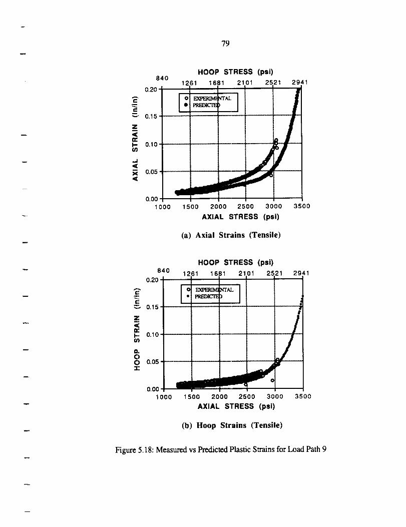
79

HOOP STRESS (psi)84o

1261 1681 2101 2521 29410.20

•_ • PIU_ZcI'E ).-= -- t

--.o.15._z.... ' ......' ** -----"

t_l--,__l0.10 _ /

0.05 ..... _'_

0.00

1000 1500 2000 2500 3000 3500

AXIAL STRESS (psi)


840

0.20

=:om.

C:_ 0.15

z

I-- 0.10U)

G.OO 0.05 r3"

0.00

1000

HOOP STRESS (psi)

1281 1681 2101 2521 2941

o _ _I"AL

• PREDlt-'FE_)q

/

1500 2000 2500 3000 3500

AXIAL STRESS (psi)



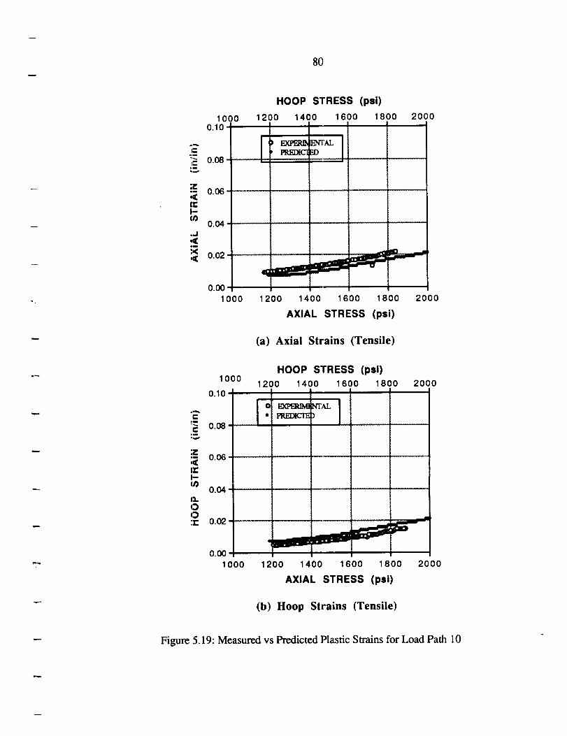
80

J

-.[

.(

)-

..I

x_C

HOOP STRESS (psi)

1000 1200 1400 1600 1800 20000.10 - I I I I

0.08

0.06

0.04

0.02

0._

1000

ENTALED

I

1200 1400 1600 1800 2000

AXIAL STRESS (psi)


C:u

C,i

Z,K1=F-¢/)

Q.

OO

1000

0.10 -

0.08

0.06

0.04

0.02

HOOP STRESS (psi)1200 1400 1600 1800

I

o! _ _/_

2000

0.00 "_

1000 1200 1400 1600 1800 2000

AXIAL STRESS (psi)



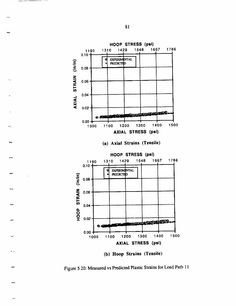
81

r..

A

e-.m

e-

Zm

<mrk-

<m

X

A

m

zm

<n-k-o_

O.OOq-

I0.10

0.08

0.06

0.04

0.02

0.00

90 13I

O

I

I

000 1

HOOP STRESS (psi)

0 1429 1548 1667I

,_TALD

O0 1200 1300

AXIAL STRESS

1786

_,oa

1 400 1 i00

(psi)


11900.10

0.08 ....

0.06"

0.04

0.02

0.00

1 )00

HOOP STRESS (psi)

1310 1429 1548 1667I

i

© EX]_UM* PPJ_CTI

I

_rAL

_a

1786

00 1200 1300 1400 1500

AXIAL STRESS (psi)


Figure 5,20: Measured vs Predicted Plastic Strains for Load Path 11

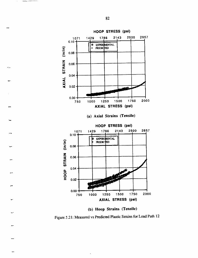
82

10710.10 -

A

C°_

¢ 0.08°m

HOOP STRESS (psi)

1429 1786 2143 2500

0 EXP_ _TAL

• PR_( FED

Zo.o6 .................

I-

,-I

I

X,K

0.04 ............

0.02

a0.00

750 1000

2857

J

1250 1500 1750 2000

AXIAL STRESS (psi)


10710.10

A

e-,m

¢ 0.08

HOOP STRESS (psi)

1429 1786 2143 2500 2857

!-O EXP_ _TAL

Z0.06............. ----,

= /_ ,.° .

0.04 ................

°0_" 0.02 =

0.00750 1000 1250 1500 1750 2000

AXIAL STRESS (psi)



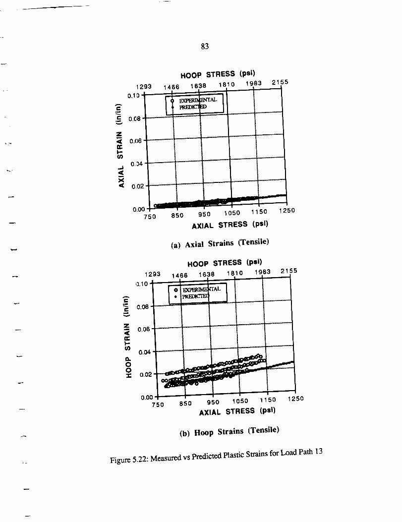
83

HOOP STRESS (psi)

0.00750 850

1983 2 55

250950 1050 1 50

AXIAL STRESS (psi)


HOOP STRESS (psi)

1293 1466 1638 1810 1983 2 55__._._.._ --= ._-_-

0.10 _ -_---_- ---) EXP_ _ 'AL

0.08 _ _'=1

_o= 0.06 ......

°o.o i===1=11=====

0.00 "P_-r_ '750 850 950 1 150 1 50 250

AXIAL STRESS (psi)



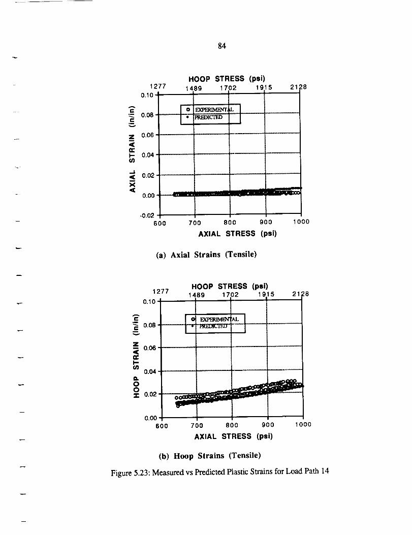
84

1277HOOP STRESS (psi)

1489 17102 1915

• I_J_ICTED

2128

J.

600 700 800 900 1000

AXIAL STRESS (psi)


1277

0.10

HOOP STRESS (psi)1489 1702 1915

e Exmu_m_• L"[,(,.]P_.J_l ]_.,u

Cm

"'.. 0.08C

m

-= 0.06 ..........

I-

0.04

00'T" 0.02

AL

21 28

0.00600 700 800 900 1000

AXIAL STRESS (psi)



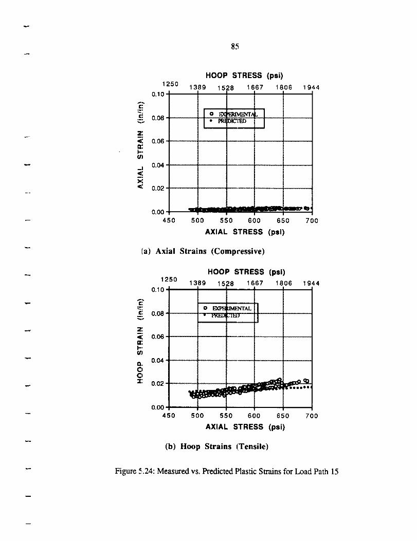
85

£,

2:m°

I-,(/I

-!<,'m°

1250

0.10

0.08

HOOP STRESS (psi)

1389 1528 1667 1806 1 944t

O EX 1_g_lT/_* RU_

0.06 ...........................................................................................

0.04 ............................................

0.02

0.00

450 700I

500 550 600 650

AXIAL STRESS (psi)

(a) Axial Strains (Compressive)


1389 1528 1667 1806 19440.10 • I i I I

£: [•-_: o EX_ HM]_ITAL..=i 0.08- • _LI_J

Z_,

0.06 ...... _.......

I=..

0.04

O 0.02

0.00

450 500 550 600 650 700

AXIAL STRESS (psi)


Figure 5.24: Measured vs. Predicted Plastic Strains for Load Path 15

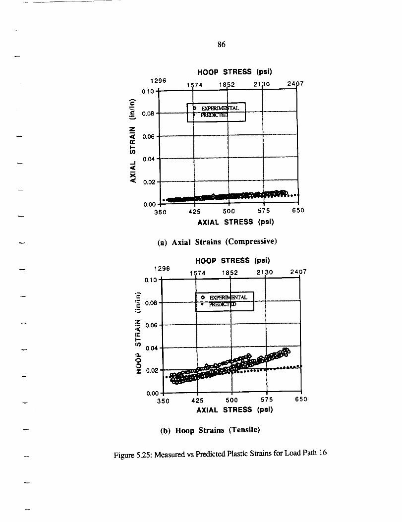
1296

0.10

t-°_

_ 0.178

zI

,_ 0.06

I-

86

_1

m

X

0.04

0.02

0.00

I,=

I_ __rALp PREI)I(,_II_I.

HOOP STRESS (psi)

;74 1852 21t3024)7

_=,00

350 425 500 575

AXIAL STRESS (psi)

650



1 i74 1852 2130 24070.10

= o EXPERI]vENTAL='_ 0.08 • t,ite_/_n_,.u ......,D

Z 0.06

;_ 0.04 ....

0.00350 425 500 575 650

AXIAL STRESS (psi)



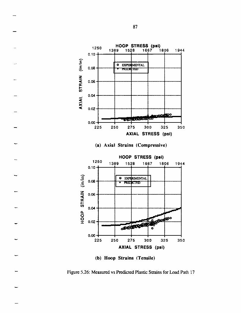
87

P,I

°m

Zm.

4_

I-,

ml

4:

4:

1250

0.10

0.08 ¸

0.06

0.04

0.02

0.00

225

HOOP STRESS (psi)1389 1528 1667 1806 1944

I I I I

O EXPI_ [Mt_WAL• _ :I]P.JJ

i i250 275 300 325 350

AXIAL STRESS (psi)


o-e,,

_w

,,w

zoh

F-ct_

[LOO:E

1250

0.10'

0.08

0.06

0.04

0.02

0.00

225

HOOP STRESS (psi)

1389 1528 1667 1806 1944

........

250 275 300 325 350

AXIAL STRESS (psi)


4" oFigure ._.26. Measured vs Predicted Plastic Strains for Load Path 17

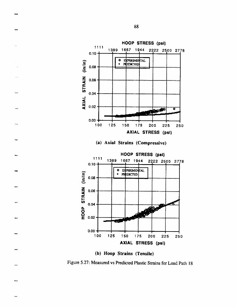
88

1111

0.10

HOOP STRESS (psi)

1389 1667 1944 2222 2500 2778

_._ o E_TAL

"" 0.08

Z0.06

ft.I-

0.04 .............

<X,1( 0.02 ....

_r/

0.00'

100 125 150 175 200 225 250

AXIAL STRESS (psi)


1111

0.10

A

r-0.08t-

,m

z-- 0.06

rek-

0.04O=OO_" 0.02,

HOOP STRESS (psi)

1389 1667 1944 2222 2500 2778

o _ m_ rAL• _ -_%'I'ED

0.00"

100 125 150 175 200 225 250

AXIAL STRESS (psi)


Figure 5.27: Measured vs Predicted Plastic Swains for Load Path 18

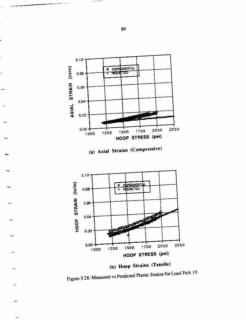
89

0.10

0.08

0.06"

0.00'1000 1250 1500 1750 2000

HOOP STRESS (psi)


2250

1000 12502000 '.250

HOOP STRESS (psi)


Figure 528: Measured vs Predicted Plastic Strains for Load Path 19

90

comparedwith resultsmeasuredduring threerepeatedtests(exceptionsareFigs 5.11 and 5.28,

which show results for four repeated tests along load paths 1 and 19, respectively). Finally, note

that all strains are plotted as positive values. The actual algebraic sign in each case is noted in the

figure caption.

The comparison between measurement and prediction is considered suprisingly good, since

these predictions are based on the Prandtl-Reuss equations, which are strictly valid only for

initially isotropic materials. Nevertheless, in most cases the predicted response falls within the data

scatter. The greatest errors are the hoop strain predictions for the f'trst few load paths (i.e., part b

in Figure 5.11 through 5.15, corresponding to load paths 1 - 6). In these cases the predicted hoop

strains at high stress levels fall below the measured hoop strains. It is believed that these

discrepancies are due to necking of the specimen. That is, for near-uniaxial loadings and at high

stresses the specimen began to neck, resulting in an unstable increase in the measured hoop strain.

The Prandtl-Reuss eq_Jations do not account for the necking phenomena, and hence the predicted

hoop strains are lower than measured in these cases.

Discussion of Pre- and Post-Yield Behavior

On the basis of the results discussed above, it has been concluded that the pre-yield behavior of

high-density polyethylene in extruded tubular form is anisotropic (i.e., transversely isotropic), and

yet the post-yield behavior is effectively isotropic. Two hypotheses which may explain this

behavior have been considered. In the first hypothesis the polymer is visualized as consisting of

stiff crystalline region _, completely surrounded by relatively flexible amorphous material. Upon

the application of elastic stress levels, motions/distortions occur at the molecular level in both the

amorphous and crystalline regions of the polymer. Since the crystalline regions were oriented

91

during the extrusion process,the initial elastic responseis anisotropic. Now, as the load is

increasedandplastic stresslevelsareinduced,the molecularmotionsin the crystalline regions

reachamaximum.All additionalstrainsareassociated with molecular motions which occur within

the amorphous regions alone. Hence, the post-yield behavior is isotropic. If this hypothesis is

valid, then no increase in the degree of crystallinity would occur as a result of the strain levels

imposed, although the crystalline regions may become reoriented. Orientation of the crystalline

regions due to high levels of stress (or strain) certainly occurs for polyethylene; the initial

orientation of the as-received tubular specimens was induced during the extrusion process, for

example. However, the strains levels induced during this study (which in all cases were < 20%)

are relatively modest compared to those encountered in the extrusion process (in which strains on

the order of several hundred l:a.'rcent are typically imposed).

In the second hypothesi,; the elastic response is again due to molecular motions within

amorphous and crystalline regions of the polymer, and hence the elastic response is anisotropic.

However, as plastic stress levels are reached additional stress- (or strain-) induced crystallization of

the polyethylene molecular structure occurs, such that initially amorphous regions become

crystallized. In this second hypothesis the crystalline regions are oriented along the prevailing

maximum stress or strain direction, and hence the post-yield response is identical for all load paths.

If this second hypothesis is valid, then the degree of crystaUinity would increase as a result of

plastic deformation. Stress-induced crystallization of polyethylene is well documeted [Rodriguez,

1989, pg 299]. However, the stress- and strain-levels associated with these documented cases are

far higher than those imposed in this study. Thus, it is unclear whether this mechanism can

account for the isotropic post-yield behavior observed during the present study.

CHAPTER 6: SUMMARY AND CONCLUSIONS

This study was devoted to an experimental and analytical evaluation of the yield and post-

yield behavior of high-density polyethylene, a semi-crystalline thermoplastic. Polyethylene was

selected for study becau,_e it is very inexpensive and readily available in the form of thin-walled

tubes. Thin-walled tubular specimens were subjected to axial loads and internal pressures, such

that the specimens were subjected to a known biaxial loading. A constant octahederal shear stress

rate was imposed during all tests. The measured yield and post-yield behavior was compared with

predictions based on both isotropic and anisotropic models. Of particular interest was whether

inelastic behavior was sensitive to the hydrostatic stress level.

The major achievements and conclusions reached during the study are itemized below.

(1) A suitable testing facility was designed, fabricated, assembled, and fully calibarated during

the course of the study. One of the unique features of the testing apparatus is a pressure control

system which allows the internal pressure to be increased at a user-defined rate, such that the

octahedral shear stress induced in the tube wall is increased at a user-defined rate. A data

aquisition system utilizing Labview software package and Macintosh 1I computer was developed

and used to collect data automaticaUy. The system is fully operational, and will be used during the

coming year to study the mechanical behavior of other engineering thermoplastic polymers.

(2) An annealing process for use with extruded high-density polyethylene tubes was

developed. Experimental measurements show that the annealing process reduces the residual

stresses induced during the extrusion process to minimal levels. However, the annealed

polyethylene specimens were found to exhibit a pronounced anisotropy. A 30% difference in

93

Young'smodulusfor the a_ial and hoop directions existed in the annealed specimens, for example.

Thus, the annealing process removed residual stresses, but did not remove or minimize anisotropic

material behavior. The anisotropic elastic behavior of high-density polyethylene is clearly due to

the semi-crystalline nature of molecular structure of this polymer.

(3) An effort was made to determine whether relatively simple isotropic yield criterion could be

used to predict yielding to within engineering accuracies. Predictions obtained using the Von

Mises and Pressure-Modified Von Mises criteria were compared with the measured data. Neither

of these models adequately predicted the experimental results. It is likely that this conclusion will

hold for other semi-crystalline thermoplastics of current structural interest (e.g.,

polyetheretherketone or polyamide), which can also exhibit a pronounced anisotropy.

(4) The tubular specimens were subsequently treated as transversely isotropic materials, with

the principal material coordinate system defined by the axial and hoop directions. Predictions

obtained using two anisotropic yield criteria (the Tsai-Hill and Pressure-modified Tsai-HiU criteria)

were then compared with the measured data. Yielding was best predicted by the Pressure-

Modified Tsai-HiU criterion, which indicates that the yield behavior of high-density polyethylene is

both anisotropic and sens:ttive to the hydrostatic stress state. It was deduced that the compressive-

to-tensile yield strength ratio of high density polyethylene is 1.11, which compares very well with

previously reported measurements.

(5) An attempt to model the post-yield behavior using the power law were made. Both an

isotropic form as well as an anisotrpic form was used. Neither power law formulation adequately

modeled the post-yield behavior, in both cases the strength coefficient M and the strain hardening

exponent n varied substmltially, depending on load path.

94

(6) Thepost-yieldbehaviorwasbestpredictedusingthe isotropic form of thePrandtl-Reuss

equations. This was an unexpectedand suprising result, since the initiation of yielding was

sensitiveto both theanisotropicnatureof thepolyethylenetubesandthehydrostaticstresslevel.

Neitherof thesefactorsareincludedin thePrandtl-Reussformulation. Thepost-yieldbehaviorof

polyethyleneis essentiallyisotropic,eventhoughtheinitial elasticresponseis anisotropic.

Two possibleexplanationsof the isotropicpost-yieldresponsehavebeenproposed.In the

first hypothesisit is suggestedthat molecular motions associatedwith plastic strainsoccur

primarily within the amorphousregionsof the polymer, and hencethe post-yield behavior is

effectively isotropic. If this hypothesisis valid, thenno increasein the degreeof crystallinity

wouldoccurasaresultof plasticdeformation.

In the secondhypothesisit is suggestedthat stress-inducedcrystallizationof theamorphous

regionsof themolecularstructureoccurs,andfurtherthatduringtheloadingprocessthecrystalline

regionsbecomeorientedin theprevailingdirectionof maximumstressor strain. Thereforethe

post-yield responsewould be identical for all load pathsconsideredduring this study. If this

secondhypothesisis valid, then the degree of crystallinity would increase as a result of plastic

deformation. Monitoring the degree of crystallinity before and after testing, as well as the

orientation of the crystalline regions, may provide a means of determining whether either of these

hypotheses is valid.

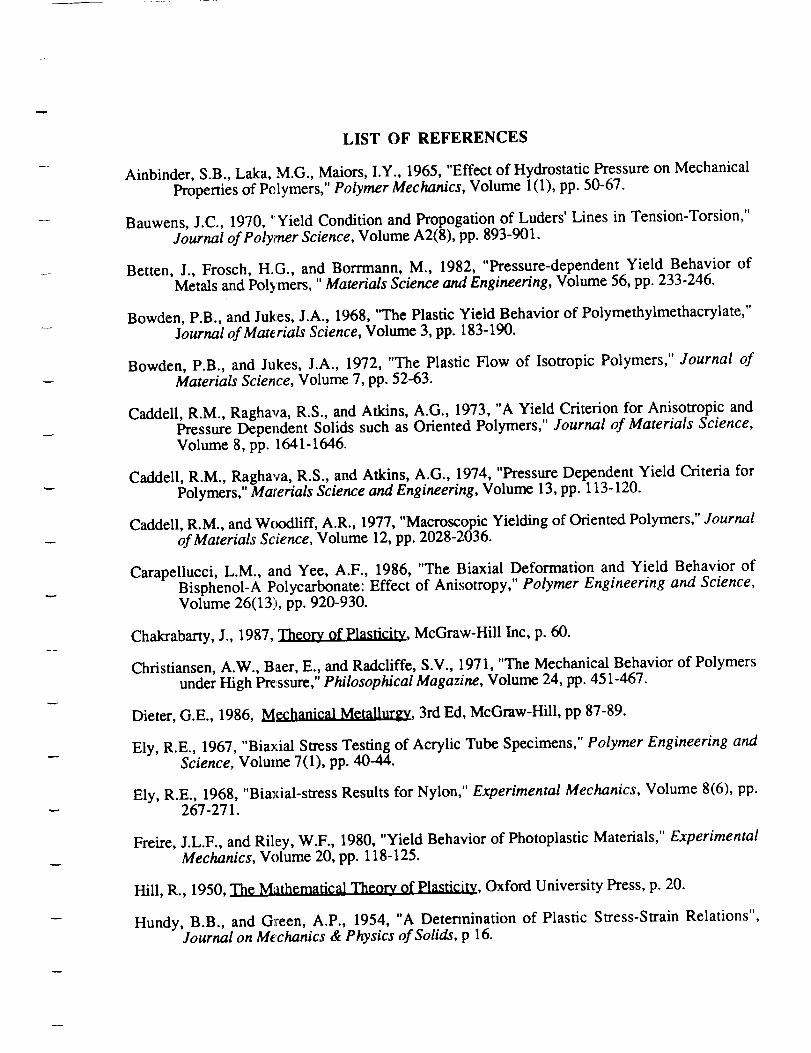
LIST OF REFERENCES

Ainbinder, S.B., Laka, M.G., Maiors, I.Y., 1965, "Effect of Hydrostatic Pressure on Mechanical

Properties of Pelymers," Polymer Mechanics, Volume 1(1), pp. 50-67.

Bauwens, J.C., 1970, "Yield Condition and Propogation of Luders' Lines in Tension-Torsion,"Journal of Polymer Science, Volume A2(8), pp. 893-901.

Betten, J., Frosch, H.G., and Borrmann, M., 1982, "Pressure-dependent Yield Behavior of

Metals and Pol) mers, "Materials Science and Engineering, Volume 56, pp. 233-246.

Bowden, P.B., and Jukes, J.A., 1968, "The Plastic Yield Behavior of Polymethylmethacrylate,"

Journal of Materials Science, Volume 3, pp. 183-190.

Bowden, P.B., and Jukes, J.A., 1972, "The Plastic Flow of Isotropic Polymers," Journal ofMaterials Science, Volume 7, pp. 52-63.

Caddell, R.M., Raghava, R.S., and Atldns, A.G., 1973, "A Yield Criterion for Anisotropic andPressure Dependent Solids such as Oriented Polymers," Journal of Materials Science,

Volume 8, pp. 1641-1646.

Caddell, R.M., Raghava, R.S., and Atkins, A.G., 1974, "Pressure Dependent Yield Criteria for

Polymers," Materials Science and Engineering, Volume 13, pp. 113-120.

Caddell, R.M., and Wc_lliff, A.R., 1977, "Macroscopic Yielding of Oriented Polymers," Journal

of Materials Science, Volume 12, pp. 2028-2036.

Carapellucci, L.M., and Yee, A.F., 1986, "The Biaxial Deformation and Yield Behavior ofBisphenol-A Polycarbonate: Effect of Anisotropy," Polymer Engineering and Science,Volume 26(13), pp. 920-930.

Chakrabarty, J., 1987, Theory_ of Plasticity, McGraw-Hill Inc, p. 60.

Christiansen, A.W., Baer, E., and Radcliffe, S.V., 1971, "The Mechanical Behavior of Polymersunder High Pressure," Philosophical Magazine, Volume 24, pp. 451-467.

Dieter, G.E., 1986, _lechanical Metallurgy, 3rd Ed, McGraw-Hill, pp 87-89.

Ely, R.E., 1967, "Biaxial Stress Testing of Acrylic Tube Specimens," Polymer Engineering andScience, Volume 7(1), pp. 40-44.

Ely, R.E., 1968, "Biaxial-stress Results for Nylon," Experimental Mechanics, Volume 8(6), pp.267-271.

Freire, J.L.F., and Riley, W.F., 1980, "Yield Behavior of Photoplastic Materials," ExperimentalMechanics, Volume 20, pp. 118-125.

Hill, R., 1950, The Mathematical Theory of Plasticity, Oxford University Press, p. 20.

Hundy, B.B., and Green, A.P., 1954, "A Determination of Plastic Stress-Strain Relations",Journal on Mechanics & Physics of Solids, p 16.

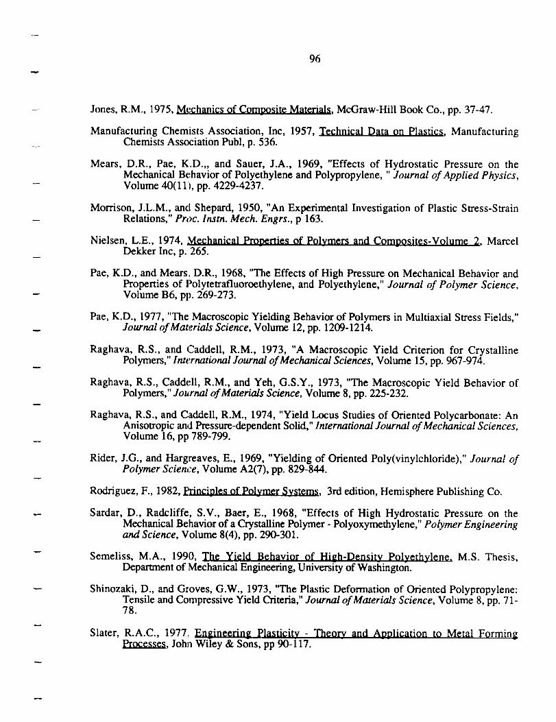
96

Jones,R.M., 1975,Mechanics of Composite Materials, McGraw-Hill Book Co., pp. 37-47.

Manufacturing Chemists Association, Inc, 1957, Technical Data on Plastics, ManufacturingChemists Association Publ, p. 536.

Mears, D.R., Pae, K.D.,, and Sauer, J.A., 1969, "Effects of Hydrostatic Pressure on theMechanical Behavior of Polyethylene and Polypropylene, " Journal of Applied Physics,Volume 40(11), pp. 4229-4237.

Morrison, J.L.M., and Shepard, 1950, "An Experimental Investigation of Plastic Stress-StrainRelations," Proc. Instn. Mech. Engrs., p 163.

Nielsen, L.E., 1974, Mechanical Prot)erties of Polymers and Composites-Volume 2, MarcelDekker Inc, p. 265.

Pae, K.D., and Mears, D.R., 1968, "The Effects of High Pressure on Mechanical Behavior andProperties of Polytetrafluoroethylene, and Polyethylene," Journal of Polymer Science,Volume B6, pp. 269-273.

Pae, K.D., 1977, "The Macroscopic Yielding Behavior of Polymers in Multiaxial Stress Fields,"Journal of Materials Science, Volume 12, pp. 1209-1214.

Raghava, R.S., and Caddell, R.M., 1973, "A Macroscopic Yield Criterion for CrystallinePolymers," International Journal of Mechanical Sciences, Volume 15, pp. 967-974.

Raghava, R.S., Caddell, R.M., and Yeh, G.S.Y., 1973, "The Macroscopic Yield Behavior ofPolymers," Journal of Materials Science, Volume 8, pp. 225-232.

Raghava, R.S., and Caddell, R.M., 1974, "Yield Locus Studies of Oriented Polycarbonate: AnAnisotropic and Pressure-dependent Solid," International Journal of Mechanical Sciences,Volume 16, pp 789-799.

Rider, J.G., and Hargreaves, E., 1969, "Yielding of Oriented Poly(vinylchloride)," Journal ofPolymer Science, Volume A2(7), pp. 829-844.

Rodriguez, F., 1982, l:_inciples of Polymer Systems, 3rd edition, Hemisphere Publishing Co.

Sardar, D., Radcliffe, S.V., Baer, E., 1968, "Effects of High Hydrostatic Pressure on theMechanical Behavior of a Crystalline Polymer - Polyoxymethylene," Polymer Engineeringand Science, Volume 8(4), pp. 290-301.

Semeliss, M.A., 1990, The Yield Behavior of Hi_h-Densitv Polvethylcrle, M.S. Thesis,Department of Mechanical Engineering, Univers_-ty of Washington.

Shinozaki, D., and Gxoves, G.W., 1973, "The Plastic Deformation of Oriented Polypropylene:Tensile and Compressive Yield Criteria," Journal of Materials Science, Volume 8, pp. 71-78.

Slater, R.A.C., 1977, Eneineering Plasticity - Theory_ and Application to Metal FormingProcesses, John Wiley & Sons, pp 90-117.

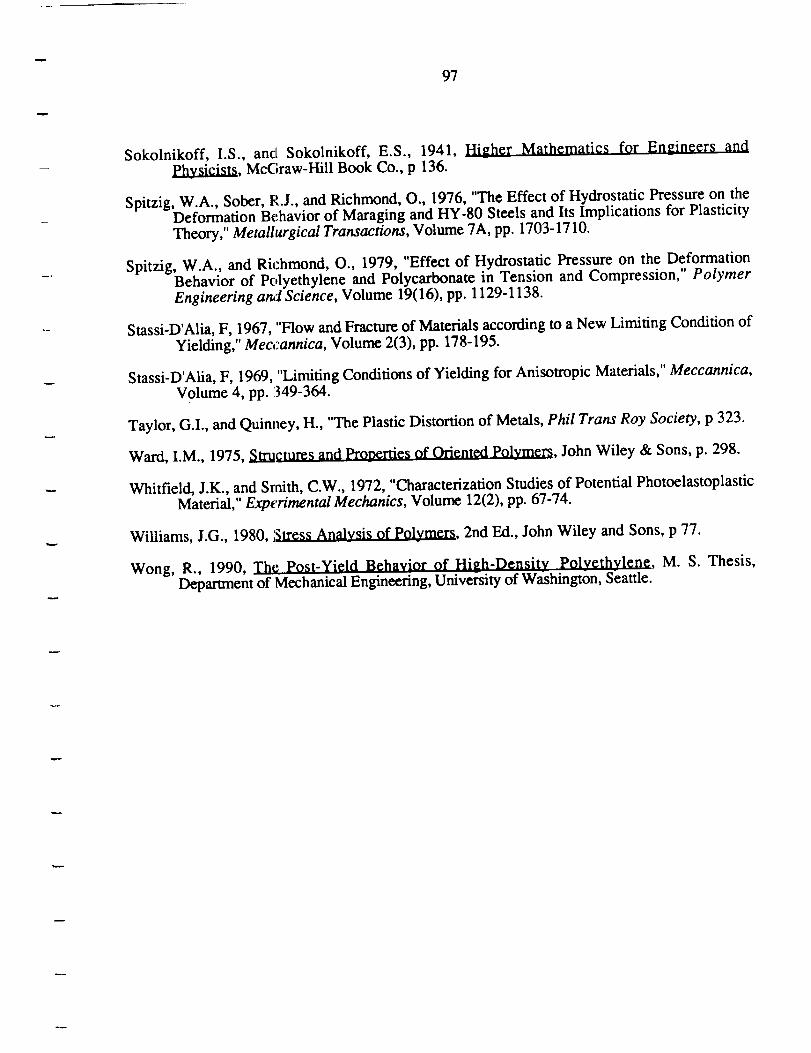
w

97

Sokolnikoff, I.S., and Sokolnikoff, E.S., 1941, Hi_her Mathematics for Engineers and

Physicists, McGraw-Hill Book Co., p 136.

Spitzig, W.A., Sober, R.J., and Richmond, O., 1976, "The Effect of Hydrostatic Pressure on theDeformation Behavior of Maraging and HY-80 Steels and Its Implications for Plasticity

Theory," Metallurgical Transactions, Volume 7A, pp. 1703-1710.

Spitzig, W.A., and Richmond, O., 1979, "Effect of Hydrostatic Pressure on the DeformationBehavior of Polyethylene and Polycarbonate in Tension and Compression," Polymer

Engineering and Science, Volume 19(16), pp. 1129-1138.

Stassi-D'Alia, F, 1967, "Flow and Fracture of Materials according to a New Limiting Condition of

Yielding," Meccannica, Volume 2(3), pp. 178-195.

Stassi-D'Alia, F, 1969, "Limiting Conditions of Yielding for Anisotropic Materials," Meccannica,

Volume 4, pp. 1349-364.

Taylor, G.I., and Quinney, H., "The Plastic Distortion of Metals, Phil Trans Roy Society, p 323.

Ward, I.M., 1975, Structures and Pro_tmrties of Oriented Polymers, John Wiley & Sons, p. 298.

Whitfield, J.K., and Smith, C.W., 1972, "Characterization Studies of Potential PhotoelastoplasticMaterial," Experimental Mechanics, Volume 12(2), pp. 67-74.

Williams, J.G., 1980, Stress Analysis of Polymers, 2nd Ed., John Wiley and Sons, p 77.

Wong, R., 1990, The Post-Yield Behavior of Hitzh-Density Polyethylene, M. S. Thesis,Department of Mechanical Engineering, University of Washington, Seattle.

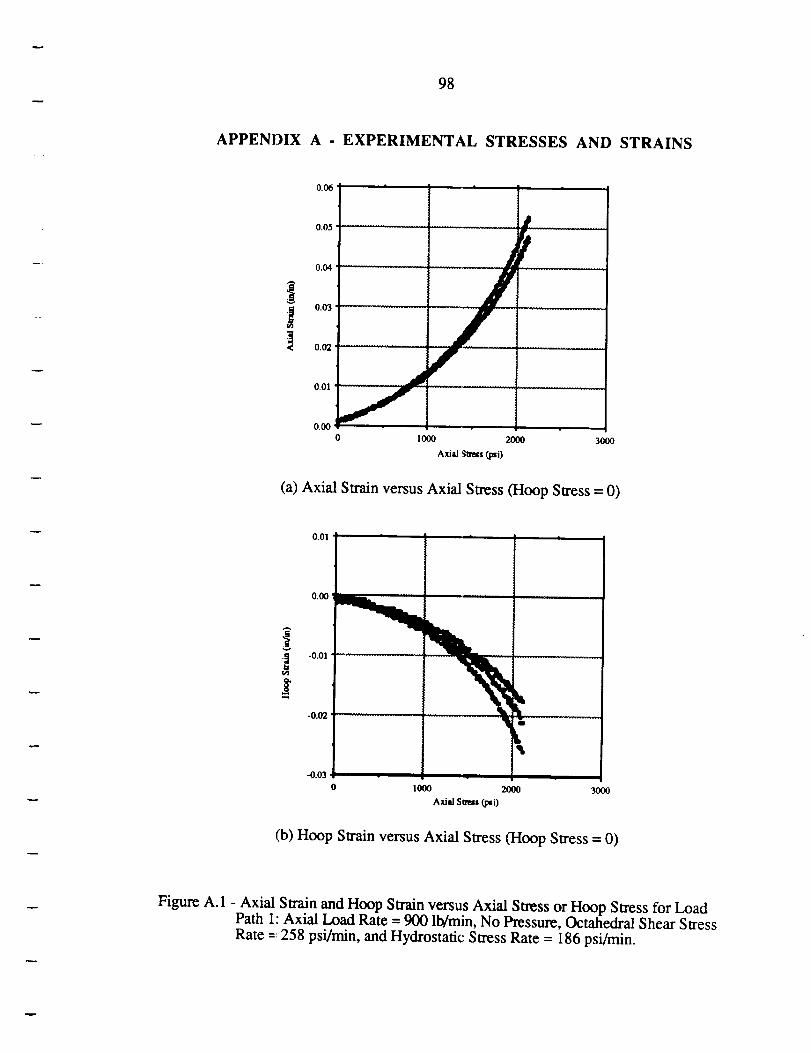
98

APPENDIX A - EXPERIMENTAL STRESSES AND STRAINS

0.06

0.05

0.04

0.1)3

0.02

0.01

0.00

I I |

...... • ................

...... jf ...............

/0 1000 2000 3000

Axial Seress (psi)

(a) Axial Strain versus Axial Stress (Hoop Stress = 0)

0.01

0.00

-0.01

-0.02

L

-0.1)3

0 1000 2000 3000

Axial Stress (psi)

(b) Hoop Strain versus Axial Stress (Hoop Stress = 0)

Figure A. 1 - Axial Swain and Hoop Swain versus Axial Stress or Hoop Stress for LoadPath 1: Axial Load Rate - 900 lb/min, No Pressure, Octahedral Shear StressRate =: 258 psi/min, and Hydrostatic Stress Rate = 186 psi/rain.

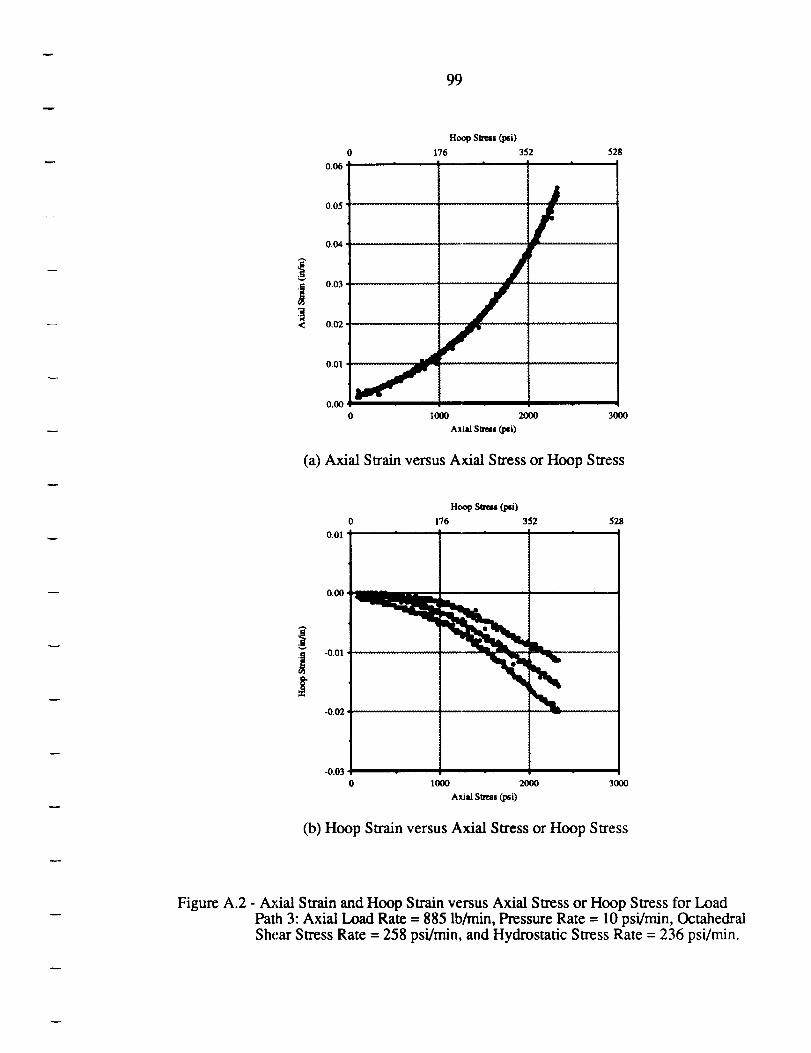
99

Hoop Stress (psi)

176 352 528

0.06 ' ' '

0.04 .......................................

< 0.02 ..... _,._

001 _

0.00 - - -

0 1000 2000 3000

Alial Stress (pli)

(a) Axial Strain versus Axial Stress or Hoop Stress

0.01

Hoop Stress (psi)

0 176 352 528

-0.01

-O.ff2 - --

-0.113

0 1000 2000 3000

^,ial Stress (psi)

(b) Hoop Strain versus Axial Stress or Hoop Stress

Figure A.2 - Axial Strain and Hoop Strain versus Axial Stress or Hoop Stress for LoadPath 3: Axial Load Rate = 885 lb/min, Pressure Rate = 10 psi/min, OctahedralShear Stress Rate = 258 psi/min, and Hydrostatic Stress Rate = 236 psi/min.

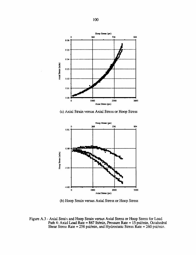
100

v

0.05

0,04

0,03

0,02

0,0!

0.00

(a) Axial Swain versus Axial Stress or Hoop Stress

Hoop Sm_s (psi)

0 268 536 804

{L01 ' ' '

-0,02

0 I000 2000 301)0

Axial Stress (psi)


Figure A.3 - Axial Strain and Hoop S_n versus Axial Stress or Hoop Stress for LoadPath 4: Axial Load Rate -- 867 lb/min, Pressure Rate = 15 psi/min, OctahedralShear Stress Rate = 258 psi/min, and Hydrostatic Stress Rate = 260 psi/min.

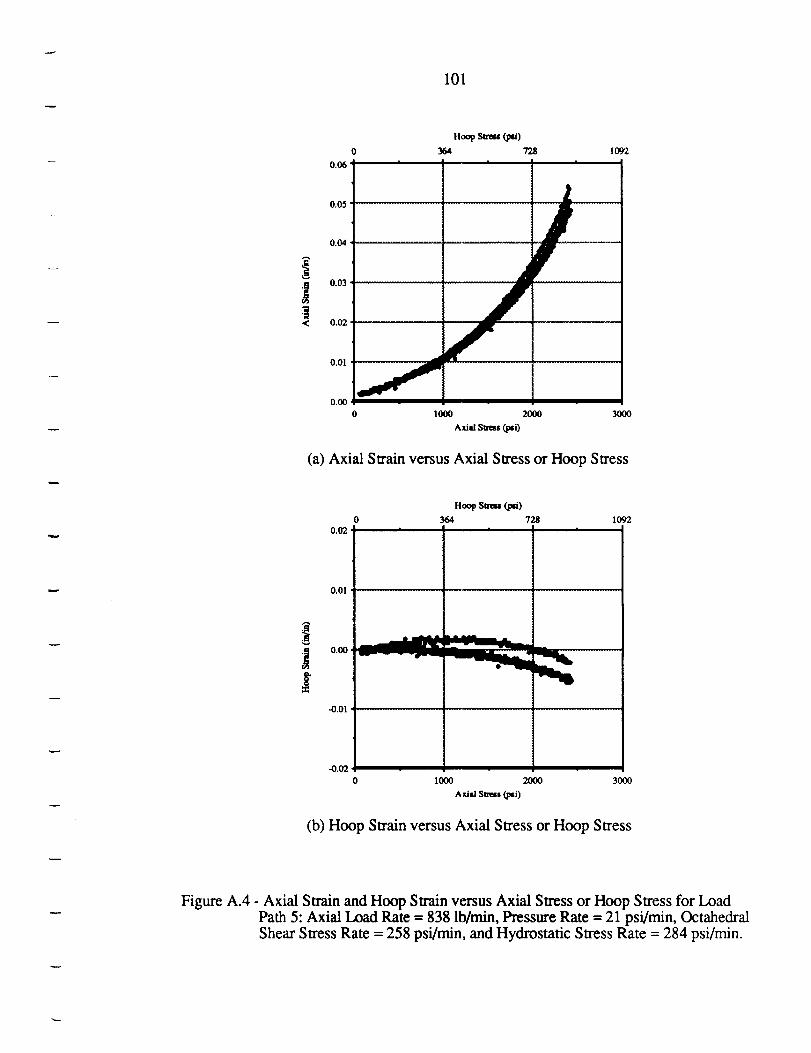
10l

0.06

0.05

0.04

0.03

< 0.02

0.01

0.00

Hoop Slreu (lxi)

0 364 728 1092|

It,

1000 2000 3000

^,iaz smm _i)


Hoop Stress (lxi)

0 364 728 10920.02 ' ' '

0.01 .....................................................................................................

ooo-0.01

-0.02

0 1000 2000 3000

A_al Sins tdxgi)


Figure A.4 - Axial Strain and Hoop Strain versus Axial Stress or Hoop Stress for LoadPath 5: Axial Load Rate = 838 lb/min, Pressure Rate = 21 psi/rnin, OctahedralShear Stress Rate = 258 psi/min, and Hydrostatic Stress Rate = 284 psi/min.

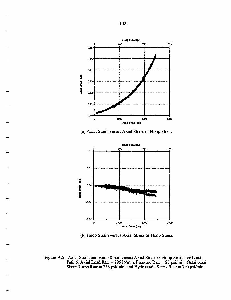
102

0.01

0.00


0.02

0.01

Hoop Stress (psi)

465 930 1395| i | |

"2 O.O0

-0.01

-0.02

0 1000 2000 3000

hxid S_ (psi)


Figure A.5 - Axial Strain and Hoop Strain versus Axial Stress or Hoop Stress for LoadPath 6: Axial Load Rate = 795 lb/min, Pressure Rate = 27 psi/min, Octahedral

Shear Stress Rate = 258 psi/min, and Hydrostatic Stress Rate = 310 psi/min.

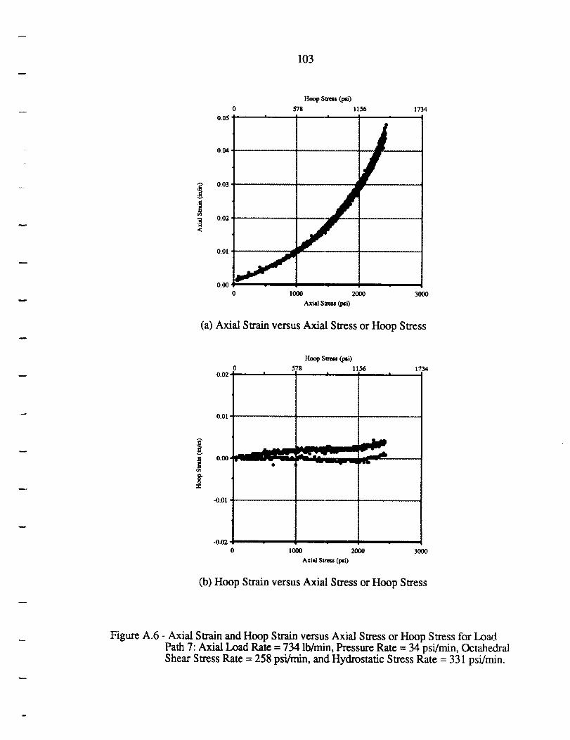
103

0.05

0.04

Hoop S_s (l_i)

0 5/8 1156 1734

................................................ I ..........

/ oo3 /,............

0°0_ .................

0.01 /. -- ...........

0.00

0 1000 2000 3000

AxialS_ (l_i)


0.02

Hoop Smum (pti)

0 578 11.56 1734

0.01

"l 0.00 •

-0.01

-0.02

0 I000 2000 3000

Axial Stress (psi)


Figure A.6 - Axial Swain and Hoop Strain versus Axial Stress or Hoop Stress for LoadPath 7: Axial Load Rate -- 734 lb/min, Pressure Rate = 34 psi/min, Octahedral

Shear Stress Rate = 258 psi/min, and Hydrostatic Stress Rate = 331 psi/min.

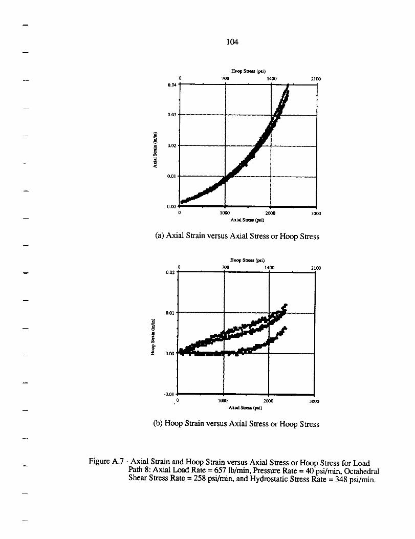
104

]

o

0.04

0.03

0.02

0.01

0.00

H¢_ Sizes (psi)

700 1400 2100

0 1000 2000 3000

Axial Sties (i_i)

(a) Axial Strain versus Atrial Stress or Hoop Stress

0.02

0.01

Hoop SII_s (l_i)

0 700 1400 2100| |

-0.01 . .

o 100o 2000 3000

Axial Sires (l_i)


Figure A.7 - Axial Swain and Hoop Swain versus Axial Stress or Hoop Stress for LoadPath 8: Axial Load Rate = 657 lb/min, Pressure Rate = 40 psi/min, OctahedralShear Stress Rate = 258 psi/min, and Hydrostatic Stress Rate = 348 psi/min.

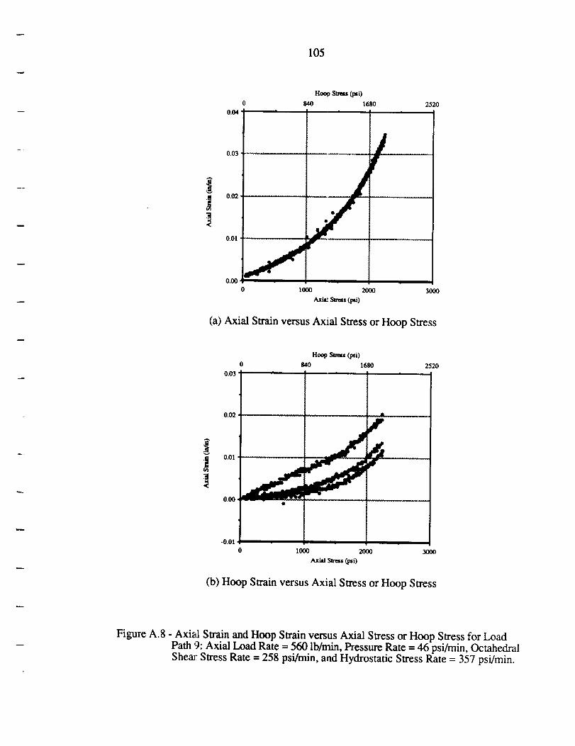
105

0.04

0.03

0.02

0.01

Hoop Stress (psi)

840 168| I t

............................ . ............. 1

2520

/0.00 _ _

0 1000 20_ 300

Ax_ Swess (psi)


Hoop Stress (psi)

0 840 1680 2520

0.03 ' '

0.02 : -_' ' ' ± _,

F

0.00

-0.01

0 1000 2000 3000

Axial Stress(p_i)

(b) Hoop Swain versus Axial Stress or Hoop Stress

Figure A.8 - Axial Strain and Hoop Strain versus Axial Stress or Hoop Stress for LoadPath 9: Axial Load Rate -- 560 lb/min, Pressure Rate = 46 psi/min, OctahedralShear Stress Rate = 258 psi/min, and Hydrostatic Stress Rate = 357 psi/min.

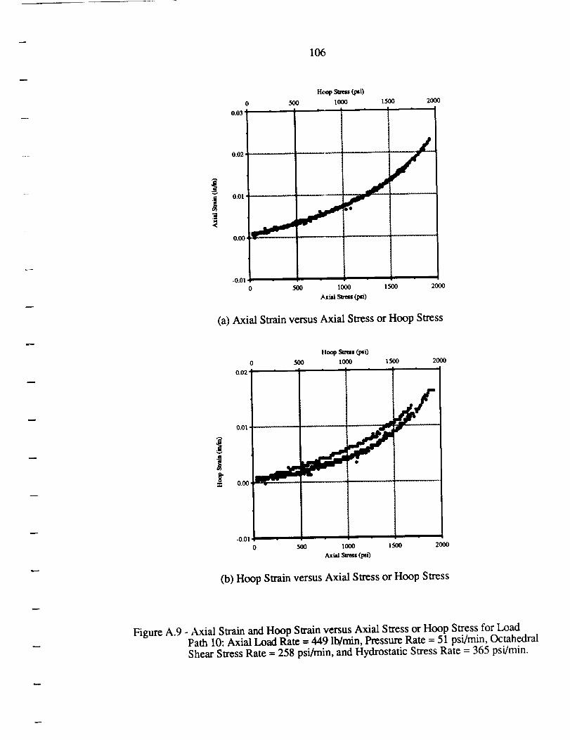
106

o

0.03"

0.02'

0.01

0.00

-0.01

Hoop Sums (psi)

500 1000 1500 2OOO

0 500 1000 1500 2000

Axial Sm_s (psi)


HoopSums (i_i)0 5oo 1000 1500 2o0o

0.02'

o.o, i.......

0.00

-0.01 - -0 5oO 1000 1500 2oo0

Axud Sta_ t_i)


Figure A.9 - Axial Strain and Hoop Strain versus Axial Stress or Hoop Stress for LoadPath 10: Axial Load Rate -- 449 lb/min, Pressure Rate = 51 psi/min, OctahedralShear Stress Rate = 258 psi/min, and Hydrostatic Stress Rate = 365 psi/min.

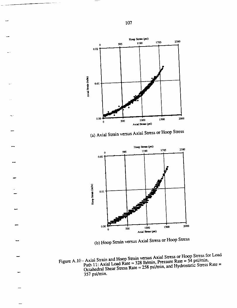
- 107

0

0.02 1

0.01

0.00

595

50O

Ho_ _s (l_i)1190 1785 2380

| | / |

o0o 5oo

A_tial _ (_i)


Itt9

m

0.02

0.01

595

ll_ _'_ (psi)1190 785 23_

| |

0._ l_o 20oo0 5_ 1000

Axill _rtta (l_i)


Figure A.10 - Axial Strain and Hoop Strain versus Axial Stress _ Hoop Stress for LoadPath 11: Axial Load Rate = 328 lb/min, Pressm'e Rate = 54 psi/rain,Octahedral Shear Stress Rate = 258 psi/rain, and Hydrostatic Stress Rate =

357 psi/rain.

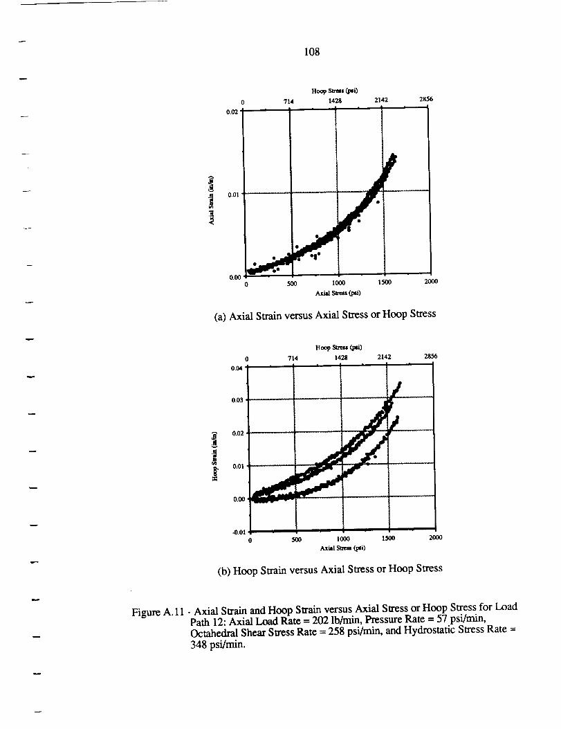
108

0.0'2

0.01

O.O0

714

Hoop S_r_I (l_i)

1428 2142 2856

500 2OOO0 5OO I00O

Axial Stress (I_i)


no,_ strm t_)0 714 14_ 2142 2856

0._'

0.03

0.02

|0.01

0.00

t .....

-0.010 500 1000 1500 2000

(b)Hoop Strain versusAxialStress orHoop Stress

Figure A. 11 - Axial Strain and Hoop Strain versus Axial Stress or Hoop Stress for LoadPath 12: Axial Load Rate = 202 lb/min, Pressure Rate = 57 psi/min,Octahedral Shear Stress Rate = 258 psi/rain, and Hydrostatic Stress Rate =

348 psi/min.

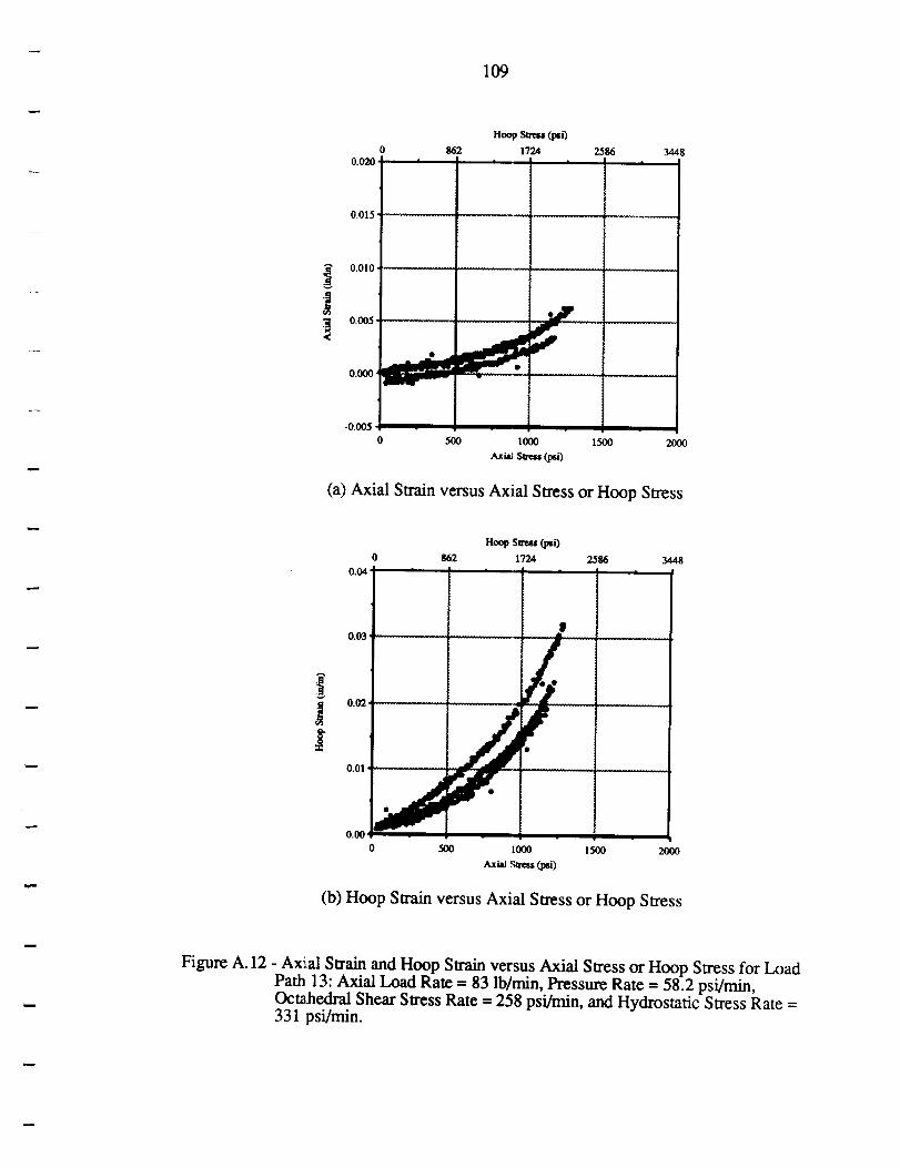
109

0.020

0.015

Hoop Stress (psi)

862 1724 2586| | |

0,010 ...........

0.005

0.000 '

344

-0.005,0 500 1000 1500

A_i_ Stress(psi)

2,000


Hoop Stress (psi)

0 g62 172,4 2586 3448

0.04 , , , L ,

0.03

0.02 .... r j__

0.01

0.00,

0 5OO 1000

tuc_ Stress (psi)

1500 2OOO


Figure A. 12 - Ax-al Strain and Hoop Strain versus Axial Stress or Hoop Stress for LoadPath 13: Axial Load Rate = 83 lb/min, Pressure Rate = 58.2 psi/min,Octahedral Shear Stress Rate = 258 psi/min, and Hydrostatic Stress Rate =331 psi/min.

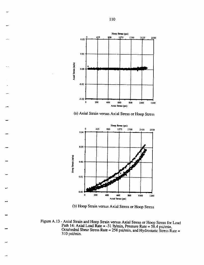
110

0.02

Hoop Sa_s (l_i)

0 425 8.$0 12"/5 I'700 2125 2550

0.01 _ ............... ! - • ........ _.............. J ........ 1.........

0.00'

4).01

L

-0.02

0 200 400 600 800

Axial S_r_s (l_i)

I000 1200


Hoop Sm_s (psi)

0 425 850 1275 1700 2125 25500.04

0.o3 ,, !.t

0.01 .......

0.00

0 2oo 60O 8OO

Axial _ (pti)

I000 1200


Figure A.13 - Axial Strain and Hoop Strain versus Axial Stress or Hoop Stress for Load

Path 14: Axial Load Rate = -31 lb/min, Pressure Rate = 58.4 psi/min,Octahe&ai Shear Stress Rate = 258 psi/min, and Hydrostatic Stress Rate =310 psi/min.

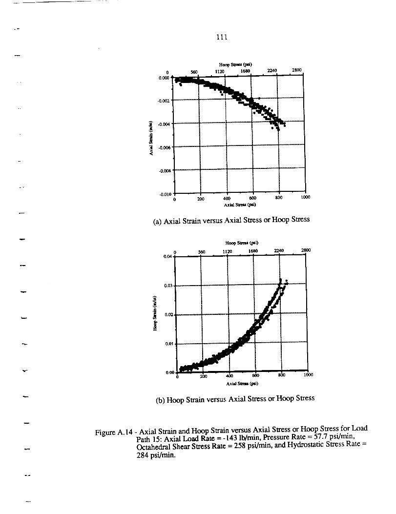
111

.t

00.o00 d

-0.002

-0.008

-0.010

56O

2OO

HoopSb-ua(_)!120 1680 224O 28OO

"'t

400 600 800 1000

Axia Str_ (pti)


0 5600.04,

0.03

0.02,

0.01

224O 28OO

0.00,

0 2o0 ,tO0 6oo 8oo 1000

Axial S_ (Imi)


Figure A. 14 - Axial Strain and Hoop Strain versus Axial Stress or Hoop Stress for LoadPath 15: Axial Load Rate = -143 lb/min, Pressure Rate = 57.7 psi/min,Octahedral Shear Stress Rate = 258 psi/min, and Hydrostatic Stress Rate =

284 psi/min.

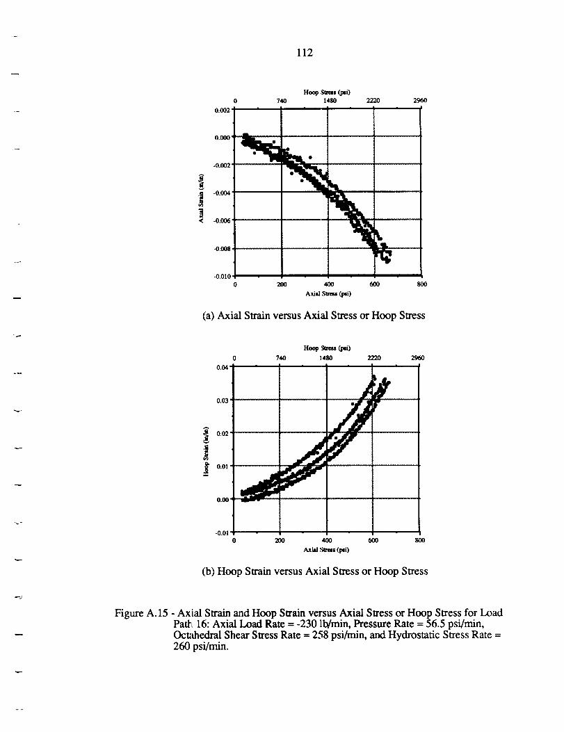
112

Hoop Sees, (psi)0 740 1480 2220

0.002

296O

oooo ....

-0.008

-0.010

0 200 400 600 800

Axial Stress (psi)


ttoq_ _ (psi)

0 740 1480 2220 2960

0.04 ,_

003......0.01'

0._' _

-0.01'0 20O 40O 600

Axial._'e_$(_i)

800


Figure A. 15 - Axial Strain and Hoop Strain versus Axial Stress or Hoop Stress for LoadPatt, 16: Axial Load Rate = -230 lb/min, Pressure Rate = 56.5 psi/min,Octathedral Shear Stress Rate = 258 psi/min, and Hydrostatic Stress Rate =260 psi/min.

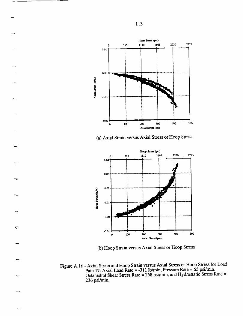
113

Hoop Sm_ (P_0

0 555 III0 1665

0.01' [

2220 2775

o.oo

-0.01

-0.02

0 I00 200 300 400 500

Axml S_e,u(l_i)


A

Hoopstress(_)0 555 1110 1665 2220 2775

0,04"

0.03'

0.02 ...........

0.01

0.00

J.

/e

-4}.01

o IOO 290 300 400 500

Axial Stre_ (psi)


Figure A. 16 - Axial Strain and Hoop Strain versus Axial Stress or Hoop Stress for LoadPath 17: Axial Load Rate = -311 lb/min, Pressure Rate = 55 psi/min,Octahedral Shear Stress Rate = 258 psi/min, and Hydrostatic Stress Rate --

236 psi/min.

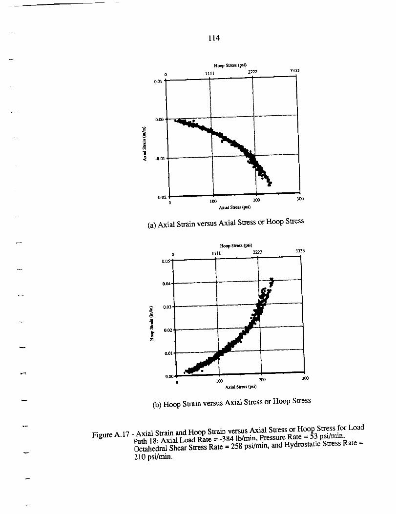
114

0.01

Hoop Stress (psi)

IIII 2222 3333n |

O.OO

-0.01 .................

.0.020 100 200

Axial Su'ess (psi)

3OO


t_

0.05"

0.04 •

0.03

0,02-

0.01

0,0_'

Hoop Stress fl_i)

1111 2222 3333i |

..... . .. '_

......i./' ....J

100 200

Stress (psi)

300


Figure A. 17 - Axial Strain and Hoop Strain versus Axial Stress or Hoop Stress for LoadPath 18: Axial Load Rate = -384 lb/min, Pressure Rate = 53 psi/rain,Octahedral Shear Stress Rate = 258 psi/rain, and Hydrostatic Stress Rate =

210 psi/rain.

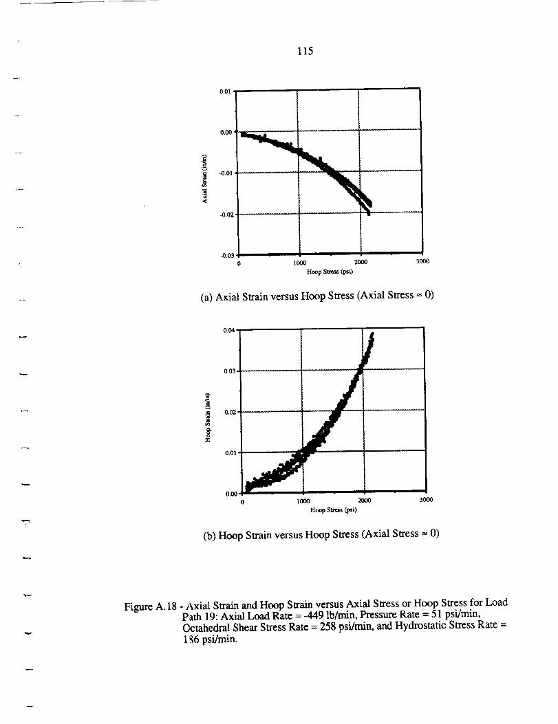
115

i

0.01 t

0.00

-0.01

-0.02

-0.03

i

1000 2000 3000

Hoop Stress (psi)

(a) Axial Strain versus Hoop Stress (Axial Stress = 0)

0.04 _

0.03

0.02 ............... /

0.01' j

0.00

0 1000 2000

Hoop SU-css (psi)

30OO

(b) Hoop Strain versus Hoop Stress (Axial Stress -- 0)

Figure A. 18 - Axial Strain and Hoop Strain versus Axial Stress or Hoop Stress for LoadPath 19: Axial Load Rate = -449 lb/rnin, Pressure Rate = 51 psi/min,Octahedral Shear Stress Rate = 258 psi/min, and Hydrostatic Stress Rate =

186 psi/min.

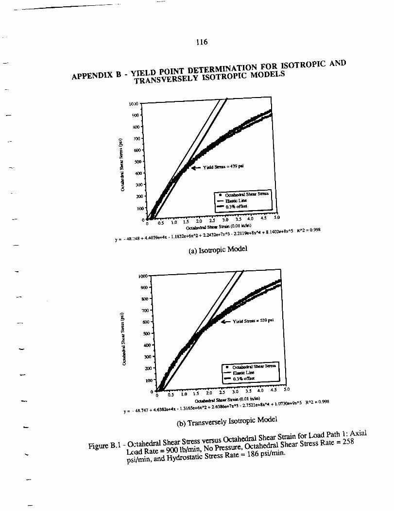
116

APPENDIX B - YIELD POINT DETERMINATION FOR ISOTROPIC ANDTRANSVERSELY ISOTROPIC MODELS

?00

60o

30O

2OO

IO0

00

She_ Satin (0.01 infm)

y = - 48.:'A8 + 4+4059e+4x - 1.1832e+6_t^2+ 2"TA32e+Tx^3 "2"2119e+SxA4 + 8"1402e+8x^5 R^2 = 0.998

(a) Isotropic Model

t000-

700

600

5OO

400

300

200

100

00 0.5 1.0 1.5


O¢*atled_ She_ Seam (0.01 tnfm)

y = . 48.747 + 4.6387.e_x - 1.3165e+6x^2 + 2"6386e+Tx^3 "2'7521e+gxA4 + l"0"730e+gx^5 R^2 = 0.998

(b) Transversely Isotropic Model

Figure B.1 - O=tahedral Shear Sffess versus Octahedra] Shear Strain for Load Path 1: AxialLx,ad Rate = 900 lb/min, No Pressure, Octahedral Shear Stress Rate = 258

psi/win, and Hydrostatic Stress Rate = 186 psi/n'fin.

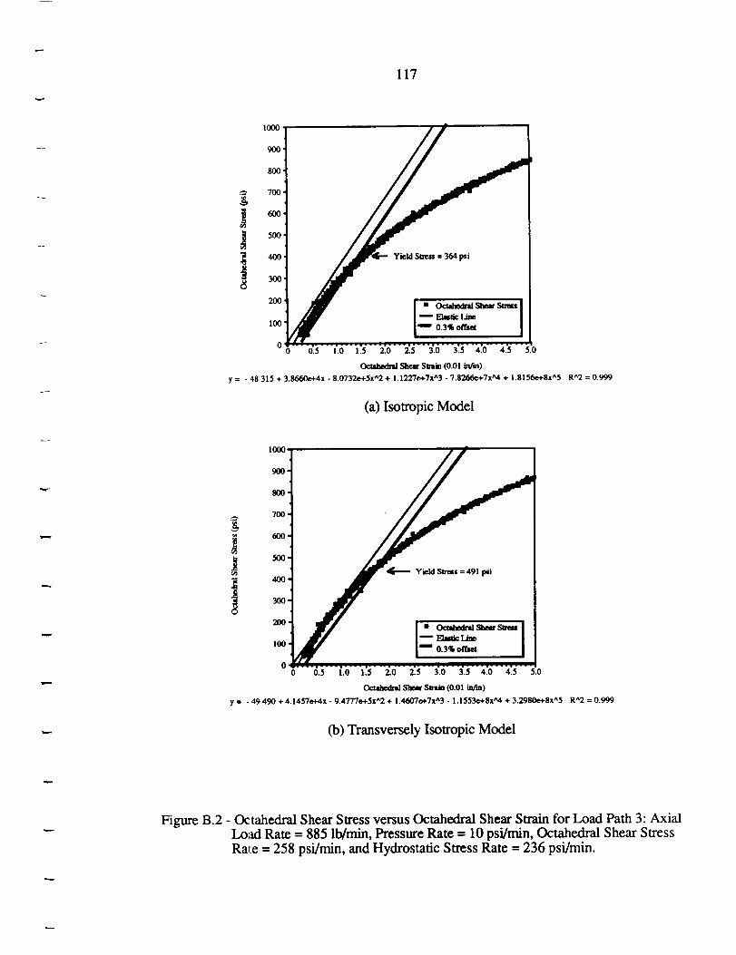
117

:1 // A

0 0,5 l.o 1.5 2.0 2.5 3.o 3.5 4.0 4.5 5.0

Ocahedni St, era Smtin (0.01 iafm)

y = - 48315 + 3.8660e+4x - 8.0'732e+Sx^2 + 1.1227¢,+'7x^3 - 7.8266e+7x'_4 + 1.8156e+Sx^5 R^2 = 0.999

(a) Isotropic Model

--'t //i700

'_..._......................J.-.._!__........!._10 0.5 1.0 1.5 2.0 2.5 3,0 3.5 4.0 4.5 5,0

Octahed_ Shear Strain (0.01 in/in)

y = - 49.490 + 4.1457e+4x - 9.4777e+5x^2 + 1,4607e+7x^3 - 1.1553e+8x'M + 3.2980e+8xA5 RA2 = 0.999


Figure B.2 - Octahedral Shear Stress versus Octahedral Shear Swain for Load Path 3: AxialLoad Rate = 885 lb/min, Pressure Rate - 10 psi/rain, Octahedral Shear Stress

Race = 258 psi/min, and Hydrostatic Stress Rate = 236 psi/min.

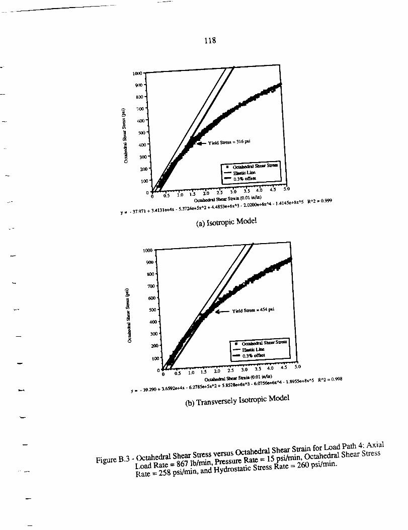
118

o

yield S_s = 316 psi

0.3% offset

o Oc_bed_d She_ s_m (o.ol infm)

y = .37971 + 3.4131e+4x-5.3724e+Sx^2+ 4"4853e+6x^3"2"_xA4 "|"4145e+Sx^5 R^2 = 0,999

(a)IsotropicModel

i

I0oo

9oo

500' [r"'-" yield S_ = 454 psi

4O0

200

I00

O'0

'[• OcU_ She_r S_

''" 0.3% ot_et

o.s :.o 1.5 _o 2,_ 3.0 3.5 4.0 4.5 5.0

y = - 39.290 + 3.6592_4x - 6.2"T85e+Sx^2 + 5'85_+6x^3 " 6"07"56e+6xA4" i.8955 ¢+8x^5 R^2 = 0.998


Figure B.3 - C)ctahedral Shear Stress versus Octahedral Shear Strain for Load Path 4: AxialLoad Rate = 867 lb/min, Pressure Rate = 15 psi/rain, Octahedral Shear Stress

Rate = 258 psi/rain, and Hydrostatic Stress Rate = 260 psi/rain.

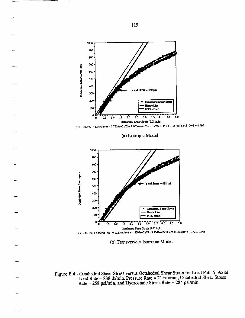
119

70O

6OO

5OO

400.

300.

200'

100

00

Yield Sb,'e_ = 360 psi

Elmlic Line |

0.3% off_ J

y = -43.490+ 3.7845e+4x-7.7524e+5x^2+ 1.0656e+7x̂ 3 "7.1793e+7xA4 + 1-3877e+Sx^5 R^2 = 0.996

(a) Isotropic Model

100o

900-

800-

Octaheda'al She.K Seam (0.01 tara)

y = • 44.135 + 4.0990e+4x - 9.1227e+Sx^2 + 1.3593e+7x^3 - 9.9346e+Tx_l + 2.1160e+Sx^5 R^2 = 0.996


Figure B.4 - Octahedral Shear Stress versus Octahedral Shear Swain for Load Path 5: AxialLoad Rate = 838 lb/min, Pressure Rate = 21 psi/min, Octahedral Shear Stress

Rate = 258 psi/min, and Hydrostatic Stress Rate = 284 psi/rain.

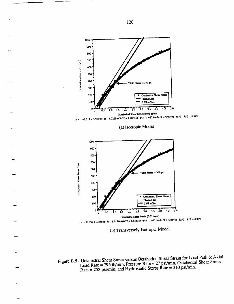
120

!i oo,300

2O0

100

0

Octahedl_lSbex Smun (0.01in/m)

y = . 49.319+ 3.9849e+4x- 8.7268e+5x^2 + 1.28"t4e+7x̂3 " 1.0273e4"8xA4+ 3"2(Ar7e+8x^5 R^2 = 0.999

(a) Isotropic Model

10¢0

900"

800.

C_

700'

600

500

400'

Yield Sue_ = 506 psi

300'

I - n'_I_ I,oo I-- o.3, I

0 0 0.5 1.0 1.5 2.0 2.5 3.0 3.5 4.0 4.5 3.0

Octahedm She_ Smda (0.01 _m)

= - 50.039 + 4.2.889e+.4x - 1.0196e +6xe'2 + 1.6451e+Tx^3 " l'4411e+Sx"_4 + 5"0549e+Sx^5 R^2 = 0.999


Figure B.5- Octahedral Shear Stress versus Octahedral Shear Strain for Load Path 6: AxialLoad Rate - 795 lb/min, Pressure Rate = 27 psi/rain, Octahedral Shear Stress

Rate = 258 psi/rain, and Hydrostatic Stress Rate = 310 psi/min.

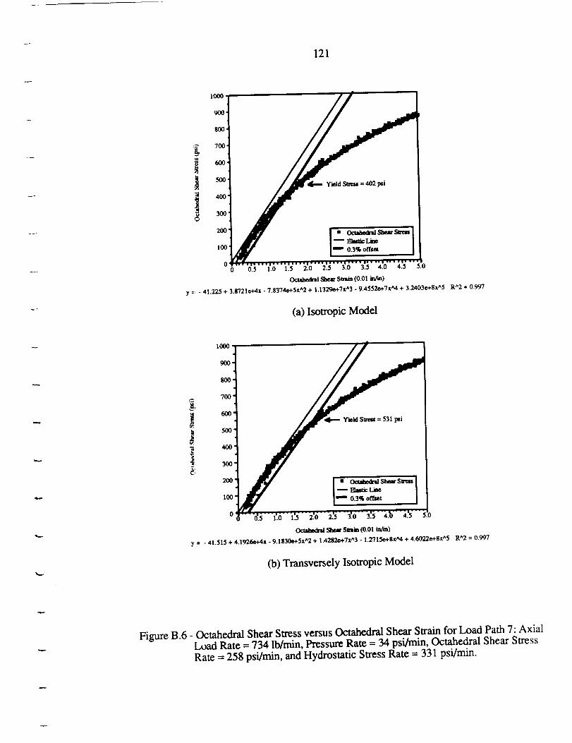
121

1000'

900'

800

O

700

6O0

500'

400'

300

200

100

0 ¸0

y =:-41.225+ 3.8"721e+4x-7.8374e+5x^2+ 1.1329e+Tx^3" 9"4552e+7xA4+ 3"2403e+8x^5

(a) Isotropic Model

R^2 = 0.99"/

1000

9OO

She_ Strain (0.01 in:m)

y : - 41.515 + 4.1926e+4x - 9.1830e+Sx^2 + 1-4282e+Tx^3 " i.2715e+8x_" + 4"6022e+8x^5 R^2 = 0.997


Figure B.6 - Octahedral Shear Stress versus Octahedral Shear Strain for Load Path 7: AxialLoad Rate = 734 lb/rnin, Pressure Rate = 34 psi/min, Octahedral Shear Stress

Rate = 258 psi/rain, and Hydrostatic Stress Rate = 331 psi/min.

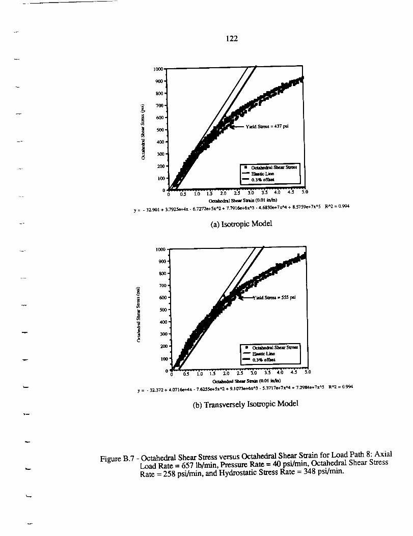
122

g

r_

600

500

_ ElmticLine

10O [ mm 0.3% ot'lg_t

00 0.5 1.0 1.5 2.0 2-5 3.0 3.5 4.0 4.5 5.0

_l Slw.an"Slrain(0.01infm)

y = - 32.901 + 3.7925e+4x - 6.7272e+5x^2 + 7.7916e+6x^3 "4.6830e+TxA4 + 8"5759e+7x^5

(a) lsotropic Model

R^2 = 0.994

1000

900"

8OO

Ea_cLm I100 0.3% oflh_ ]

00.5 1.0 1.5 2-0 2.5 3.0 3.5 4.0 4.5 5.0

Ocuam_ai Shear sm_ (o.01 iafln)

y = - 32.372 + 4.0716o¢.4x - 7.6255o+5x^2 + 9 .1073e'l'6x^3 " 5"3717°+7XA4 + 7"2984e+Tx^5 R^2 = 0.994


Figure B.7 - Octahedral Shear Stress versus Octahedral Shear Strain for Load Path 8: AxialLoad Rate = 657 lb/min, Pressure Rate -- 40 psi/min, Octahedral Shear Stress

Rate = 258 psi/min, and Hydrostatic Stress Rate = 348 psi/min.

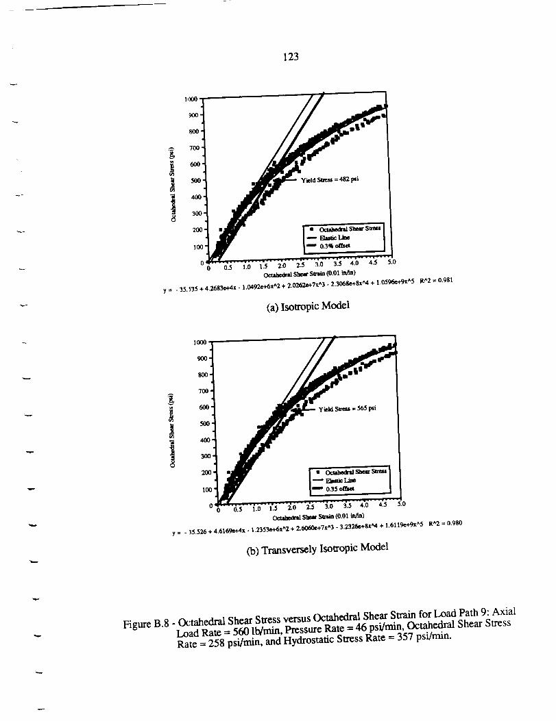
123

(a)IsotropicModel

R^2 = 0.981

1000

90O

800-

700"

600'

5OO

40O

yield Sirras = 565 psi


Figure B.8 - Octahedral Shear Stress versus Octahedral Shear Swain for Load Path 9: AxialLoad Rate - 560 lb/min, Pressure Rate = 46 psi/rain, Octahedral Shear StressRate = 258 psi/rain, and Hydrostatic Stress Rate = 357 psi/rnin.

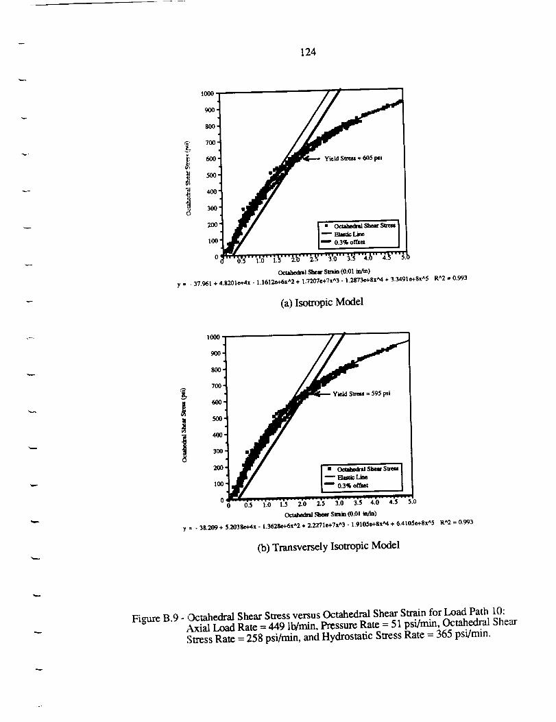
124

1000-

900-

80O

O

700

600.

200'

100"

0

Yie|d Stress = 605 psi

0.3% offset ]

_1 $heffi Smtia (0.01 infm)

y = - 37.961 + 4.8201e+,4x - 1.1612e+6x ^2 + 1.7207e+Tx^3 " l'2ff'/3e+gxA4 + 3"3491e+8x^5

(a) Isotropic Model

R^2 = 0.993

1000

9OO

800"

700"

600-!

300.

200-|

100"

Yield Su_s = 5951_i

00 0.5 1.0

y = - 38.209 + 5.2038e+,4x - 1.3628e+6x^2 + 2-2271e+7x^3 " 1.9105e+gx _, + 6 .4105e+Sx^5 R^2 = 0.993


Figure B.9 - Octahedral Shear Stress versus Octahedral Shear Strain for Load Path 10:Axial Load Rate = 449 lb/min, Pressure Rate = 51 psi/min, Octahedral Shear

Stress Rate = 258 psi/min, and Hydrostatic Stress Rate = 365 psi/min.

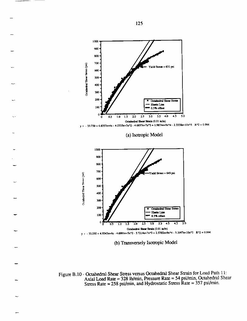
125

'_. // I

):: 63,.400 •

300

0 0.5 !.0 1.5 2.0 2.5 3.0 3.5 4.0 4.5 5.0

y = - 33."/50+ 4.6357e+.4x- 4.2335e+Sx^2-4.6837e+Tx^3+ 1.9974e+gx"_4"2"3358e+IOxA5

(a) Isotropic Model

R^2 = 0m_

-I

l:_ /7 1

"1Z_ /s = 649psi

/_'I4'/ i'-_°_'_'-I /

_ sm_ (0.01 i_n)

y = - 33.550 + 4.9345e+4x - 4.6981v+5x^2 - 5.7214e+7x^3 + 2.5702e+9z,_4 - 3.2097e+10x^5 R^2 = 0.994


Figure B.10- Octahedral Shear Stress versus Octahedral Shear Strain for Load Path 11:Axial Load Rate - 328 lb/min, Pressure Rate = 54 psi/min, Octahedral Shear


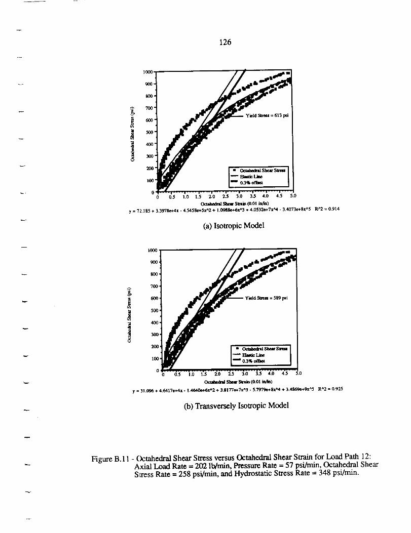
126

1oo0

900-

8oo

7oo

600"

500-

Yield S_ress = 613 psi

200

Ioo

00 0.5 1.0

y ffi72.185+ 3.3978e+4x- 4.5458e+Sx^2+ 1.0988e+6x^3+ 4.0532e+7xA4 -3.4073e+Sx^5 R^2 = 0.914

(a) Isotropic Model

o

iooo ¸

9oo

80o

7oo

600.

500,

400,

300,

200,

I00

0

y = 31.096+ 4.6417e+4x- 1.4640e+6x^2+ 3.$177e+7x^3- 5.7979e+Sx^4 + 3.4869e+9x^5 R^2 = 0.925

(b)TransverselyIsotropicModel

Figure B.11 - Octahedral Shear Stress versus Octahedral Shear Strain for Load Path 12:Axial Load Rate = 202 lb/min, Pressure Rate = 57 psi/rain, Octahedral Shear

Stress Rate = 258 psi/rain, and Hydrostatic Stress Rate = 348 psi/min.

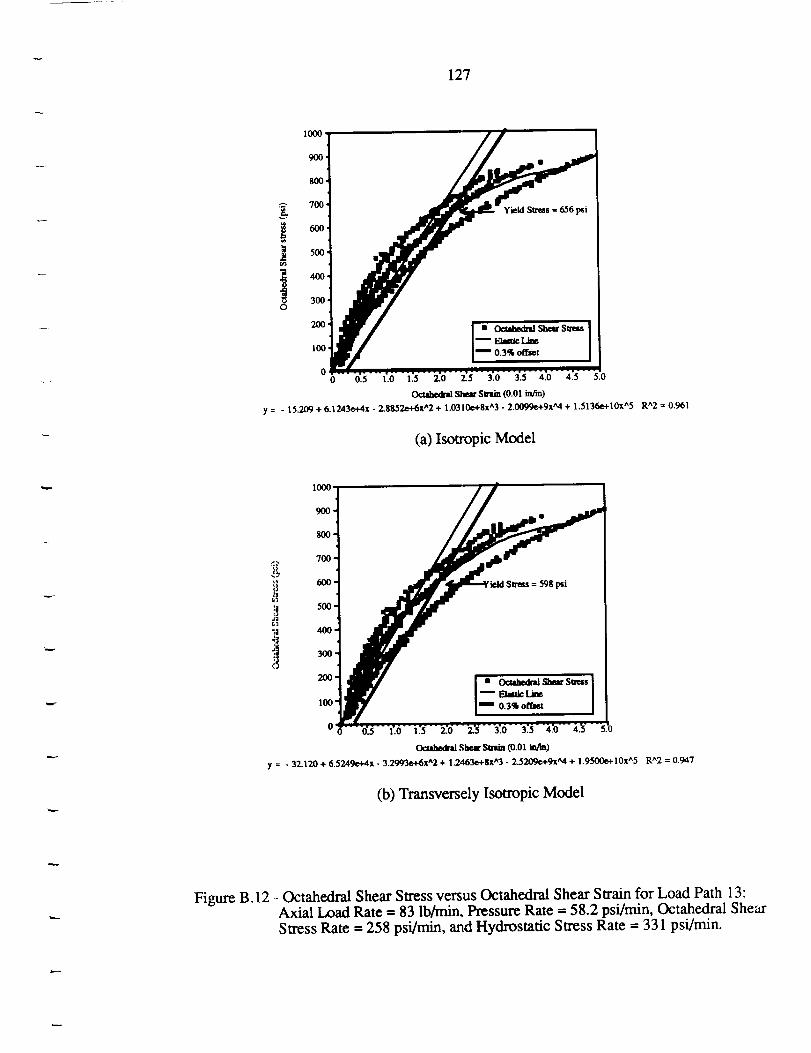
127

b

J

O

1000,

900,

800,

700

6O0

5OO

Yield Soress = 656 psi

y = - 15.209+ 6.1243e-l-4x-2.8852e+6x^2+ 1.0310e+8x^3- 2.0099e+9x'M+ 1.5136v+10x^5 R^2 = 0.961

(a) Isotropic Model

J!

900-

8130-

700-

600-

500-

400.

300.

200.

I00'

O'

psi

Octahedral She_ Strata (0.01 _ln)

y = - 32.120 + 6.5249e+4x - 3.2993e+6x^2 + 1.2463e+Sx^3 - 2.5209e+gxA4 + 1-9500e+10XA5 R^2 = 0.947


Figure B.12 - Octahedral Shear Stress versus Octahedral Shear Su'ain for Load Path 13:Axial Load Rate = 83 lb/min, Pressure Rate -- 58.2 psi/rain, Octahedral Shear

Stress Rate = 258 psi/min, and Hydrostatic Stress Rate = 331 psi/rain.

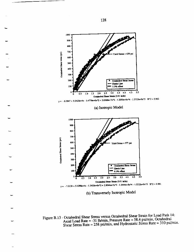
128

l

io0o

900

800.

700-

600

500

psi

I- _'_L_ IlOO

0 0 0.5 1.0 1.5 2.0 2.5 3.0 3.5 4.0 4.5 5.0

Octahedral Shear Su'a_ (0.01 in/m)

y = - 8.0947 + 5.0425e+4x - 1.4770e+6x A2+ 2.6568o+7x^3" l'2050e+gxA4 " l'5723e+9X^5 RA2 = 0.962

(a) Isotropic Model

1000,

9OO

8OO

700,

600,

500

4OO

3OO

200,

100,

00 0.5 1.0

Yield Stress = 577 i_i

1.5 2.0 2.5 3.0 3.5 4.0 4.5

OctahedrM She_ SU'tin (0.01 infm)

y = . 7.0159 + 5.1298e+4x - 1.5435e,+6r"2 + 2.9044e+7x^3 " 1'5444e+SxA4 " l'5222e+9X^5 R^2 = 0.961


Figure B.13 - Octahedral Shear Stress versus Octahedral Shear Swain for Load Path 14:Axial Load Rate = -31 lb/min, Pressure Rate - 58.4 psi/rnin, OctahedralShear Stress Rate = 258 psi/rain, and Hydrostatic Stress Rate = 310 psi/min.

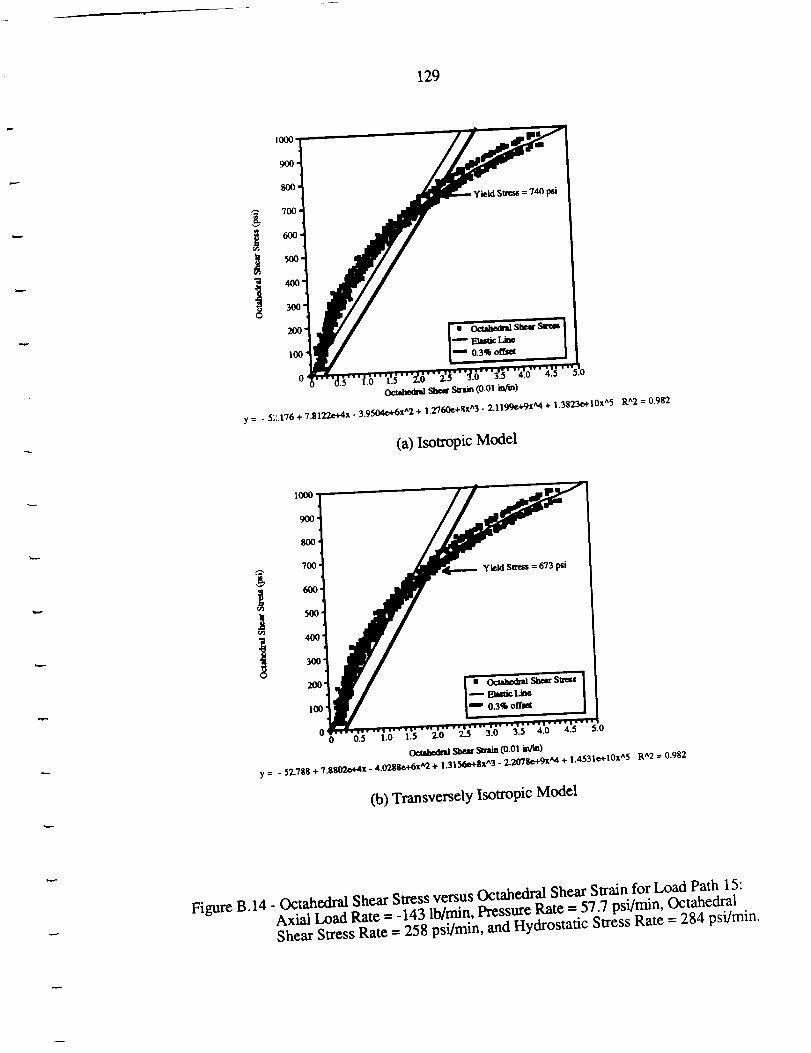
129

1000-

800,

700.

600'

500

y = . 57.176 + 7.8122e+4x - 3.950'_t'6x^2 + l'2"/60e+gx^3 " 2"l199e+9xA4 + 1"3823e+10x^5 R^2 = 0.982

(a) Isotropic Model

1000,i

900"

80o,

1

700

6O0

5O0

300'

200

100'

00

Oaahed_ SheE Sere t_.01 i_¢m)

y = - 52.788 + 7.8802e_x - 4.0288e+6x^2 + l'3156e+Sx^3 "2.2078e+gx_t + 1.4531e +10x^5 R^2 = 0.982


Figure B.14- Octahedral Shear Stress versus Octahedral Shear Strain for Load Path 15:Axial Load Rate - -143 lb/min, Pressure Rate = 57.7 psi/rain, OctahedralShear Stress Rate = 258 psi/rain, and Hydrostatic Stress Rate = 284 psi/rain.

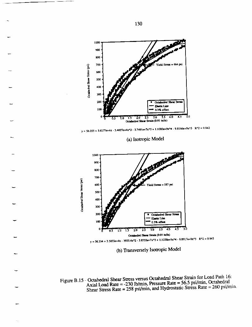
v

130

1000,

9O0

8OO

700

600

5OO

400

300

200

100

0


y = 56.055 + 3.6177e+4x - 3.40"ZTe+4x^2 " 3.7491e+7z^3 + 1.1080e+9x_t - 9.8166e+9x ^5 R^2 = 0.942

(a) Isotropic Model

1000

9oo

800,

700 ¸I

600.

500.

400,

300

200"

100"

O'

Yield Slress = 587 psi

m Octahedr_ShearStrea 1-- ElmiclJme

0.3% offNt

Octahedrll SheR S_ (0.01 tnfal)

y = 56.334 + 3.5833e+4x - 3933.4x^2 - 3 .8555e+Tx^3 + 1.1238e+9x_t - 9.8917e +9x^5 R^2 = 0.943


Figure B.15 .. Octahedral Shear Stress versus Octahedral Shear Strain for Load Path 16:Axial Load Rate = -230 lb/min, Pressure Rate -- 56.5 psi/rain, OctahedralShear Stress Rate = 258 psi/rain, and Hydrostatic Stress Rate = 260 psi/min.

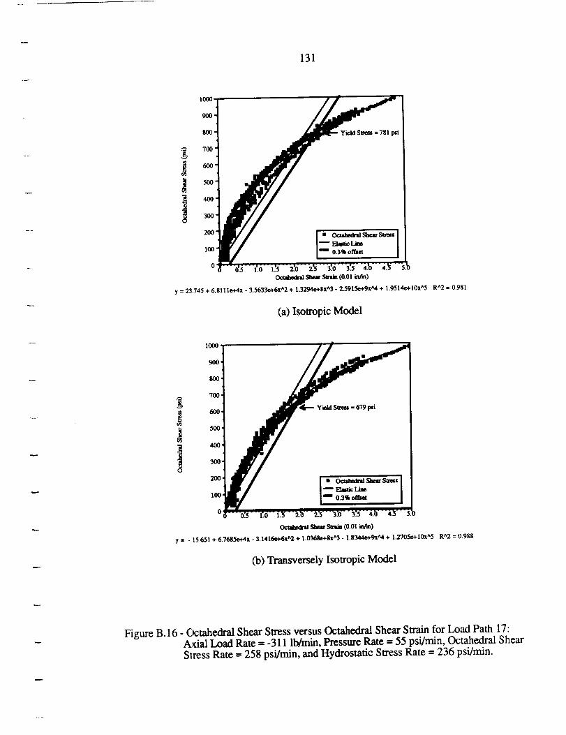
131

yield Sm_ -- 781 i_i

I000

900"

800,

700'

i °300

I• o_,_..s_.,,1oo. I- 03,o_

O'

OcUdldU'_ Sbmr Su'u_ (0.01 e_n)

y = 23.745+ 6.81110+4x-3.5633¢+6x^2+ 1.3294¢+8x^3" 2.59150+9xA4+ 1.9514¢+I0x^5

(a) IsotropicModel

R^2 = 0.981

1000

0

900 ¸

800.

700.

600.

500,

400,

300'

200i

100.

0

Yield Strea = 679 psi

Ocudlx_ Slleu Se.-i,,, (0.01 kllfm)

y = - 15.651 + 6.7685e+4x - 3.1416et6x"2 + 1.0368e+gx^3 - 1-8344e+9xA4 + 1.2705e+10x^5 R^2 = 0.988


Figure B.16 - Ocmhodral Shear Stress versus Octahedral Shear Strain for Load Path 17:Axial Load Rate -- -311 lb/min, Pressure Rate = 55 psi/rain, Octahedral Shear

Stress Rate = 258 psi/rain, and Hydrostatic Stress Rate = 236 psi/min.

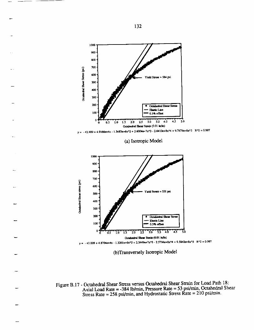
132

1000.

700

60O

5O0


I00 0.3% offset

00 0.5 1.0 1.5 2.0 2.5 3.0 3.5 4.0 4.5 5.0

Ocudaedral She_ Semin (13.01 in/m)

y = - 42,889 + 4.9166e+4x - 1.:M83e+6x^2 + 2._ 7x^3 "2.6410e+8x'_4 + 9.7674e+8x^5 R^2 = 0.997

(a) Isotropic Model

lOOO

9oo

800-

700-

600-o

500-

4O0

3OO

200"

100"

0'

Yield Seress= 551 psi

Ocahednd Shear Shin (0.0t _n)

y = - 43.009 + 4.870_+4x - 1.3261e+6x^2 + Z5449e+Tx^3 "2.5794e+gx_4 + 9.5842e+gx^5 R^2 = 0.997

(b)Transversely Isotropic Model

Figure B.17 - (k:tahedral Shear Stress versus Octahedral Shear Swain for Load Path 18:Axial Load Rate = -384 lb/min, Pressure Rate = 53 psi/rain, Octahedral Shear

Slress Rate = 258 psi/rain, and Hydrostatic Stress Rate = 210 psi/rain.

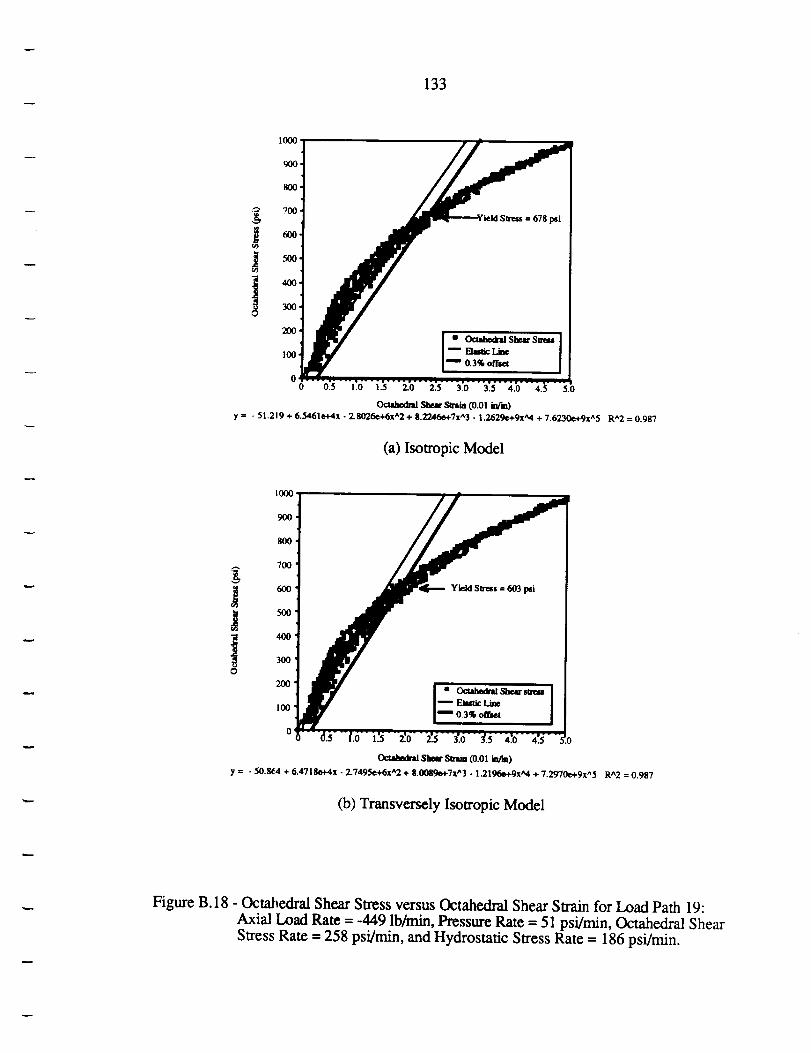
133

J

1000'

900'

800'

700'

600,

500,

400.

300"

200"

I00

00

678 p6i

y = - 51,219 + 6.5461e+4x - 2.8026e_x^2 + 8.2246o+7x^3.1.2629e+9xA4 + 7.6230e+9x^5 R^2 = 0.987

(a) Isotropic Model

IOOO

800

J

700'

600'

500

4O0

3O0

2OO

ioo

o

Yield S_'ess = 603 p_i

Octahedrtl Slur Snm (0.01 hlfm)

y = - 50._4 + 6.4718o+4x. Z7495e+6x^2 + 8.0089e+Tx^3. 1.2196e+gxA4 + 7.2970e+9x^5 R^2 = 0.987


Figure B.18 - Octahedral Shear Stress versus Octahedral Shear Strain for Load Path 19:

Axial Load Rate = -449 lb/min, Pressure Rate = 51 psi/min, Octahedral Shear


134

APPENDIX C - STANDARD DEVIATION CALCULATION

The Pressure-modified Tsai-Hill is given by:

H(c51 - ¢12)2 + F(c52 - 03) 2 + G(c3 - ell) 2 + KI(JI + K2_2 + K303 = 1 (C.1)

1 1 1

with H+G-c1T1 H+F-c2T2 G+F-c3T3

K1 CI - T1 C2- T2 K3 C3- T3- CIT1 K2- C2T2 = C3T3

testing was completed under plane stress conditions, a3 = 0, therefore:

(H + G) crl2 + (H + F) (y22 - 2H_1_2 + K1CYl + K2(Y2 = 1 (C.2)

Substituting the coefficients defined in Equation (C. 1) into Equation (C.2) results in:

_12 ¢r22 _1_2 C 1 - T1 C2 - T2C1T1 +C2T2 - _ + C1T10l + C2T2 02 = 1 (C.3)

It is assumed that the material exhibits the same compressive strength to tensile strength

ratio (S) in the 1- and 2- directions. That is, it is assumed that:

C1 C2S = T---i- - T2 (C.4)

Under this assumption, Equation (C.3) reduces to:

135

__1 2 + 02 2 t_lt_2 1 61ST12 _7_ - ST12 +- + T22 = 1 (C.5)

For a given load path of slope M, the following substitution can be made:

ol = M t_:, (C.6)

Therefore:

M2022 022 M¢I22 S-1 (1_162 t_2 )+i_2 2" S-_12 +-g-_,-'_-I + T22 =1 (C.7)

Rearranging the previous equation results in the following:

1 1/= 1 (C.8)

If the C/T ratio (S) and slope of the load path (M) are given, one can use the quadratic

equation to sol,,e for the values of hoop stress (t_2) which will satisfy the above

relationship. The values of hoop stress which are the roots of the above equation

correspond to the intersections of the Pressure-modified Tsai-Hill locus with a C/T ratio

equal to S and rite load path with the slope M. In other words, the roots of the above

equation are the yield stresses for a given load path predicted by the Pressure-modified

Tsai-Hill. Once the predicted hoop stress value (62) is known, the predicted axial stress is

equal to M times the hoop stress.

136

Example:

Given: (1) ConsiderLoad Path 4. The slope of this load path is M = 3.73.

(2) Consider the Pressure-modified Tsai-Hill with a strength ratio of S = C/T =

1.08.

(3) The tensile yield strengths in the 1- and 2- directions are T1 = 1143 psi, and

T2 = 1279 psi, as given in Table 2.

Substituting these: values for M, S, T1, and T2 into Equation (C.8) results in the following

expression:

7.783e6 (3'22 + 2.996447e 4 o2 - 1 = 0 (C.9)

This results in a value for hoop stress at yield of 340 psi, and therefore the predicted axial

stress at yield is 1268 psi.

The experimentally measured values at yield along Load Path 3 were 288 psi (02)

and 1074 psi (Ol). The standard deviation was based on the radial distance from the origin

to the point represented by the two stress values in principal stress space. The radius is

defined as:

Radius = a,/ol2 + 022 (C.IO)

Therefore the experimental radius and theoretical radius as predicted by the Pressure-

modified Tsai-HiU with a C/T ratio equal to 1.08 are:

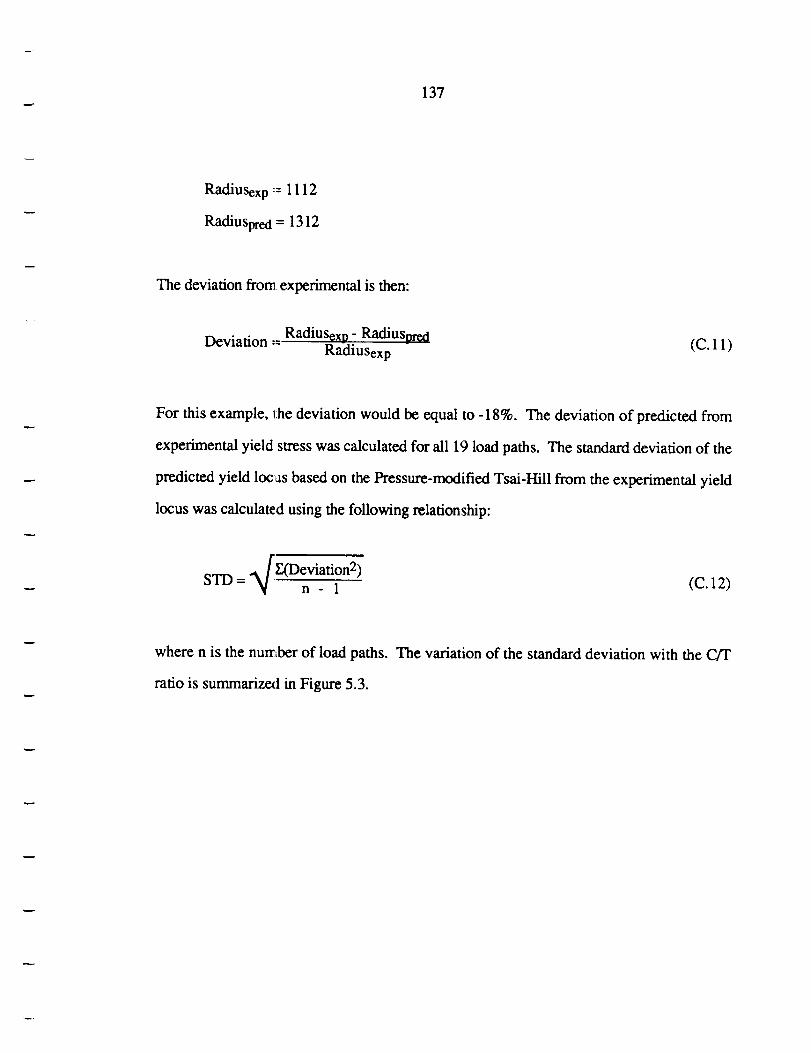
137

Radiusexp-=1112

Radiuspred= 1312

Thedeviationfromexperimentalis then:

Deviation.- Radiusexp- RadiuspredRadiusexp

(C.11)

For this example, the deviation would be equal to -18%. The deviation of predicted from

experimental yield stress was calculated for all 19 load paths. The standard deviation of the

predicted yield locas based on the Pressure-modified Tsai-Hill from the experimental yield

locus was calculated using the following relationship:

_ E(Deviation 2)STD= n- i (C.12)

where n is the number of load paths.

ratio is summarized in Figure 5.3.

The variation of the standard deviation with the C/T

Documents

The Yield and Post-Yield Behavior of by - NASA purpose of this research is to study the yield and post-yield behavior of a thermoplastic polymer subjected to biaxial stress states