Embed Size (px)
Citation preview
The XL and XSL attacks on Baby Rijndael
by
Elizabeth Kleiman
A thesis submitted to the graduate faculty
in partial fulfillment of the requirements for the degree of
MASTER OF SCIENCE
Major: Mathematics
Program of Study Committee:Clifford Bergman, Major Professor
Maria AxenovichGiora Slutzki
Iowa State University
Ames, Iowa
2005
Copyright c© Elizabeth Kleiman, 2005. All rights reserved.

ii
Graduate CollegeIowa State University
This is to certify that the master’s thesis of
Elizabeth Kleiman
has met the thesis requirements of Iowa State University
Major Professor
For the Major Program
iii
DEDICATION
To my family, for their guidance, support, love and enthusiasm. Without these things this
thesis could not have been possible.
iv
TABLE OF CONTENTS
LIST OF TABLES . . . . . . . . . . . . . . . . . . . . . . . . . . . . . . . . . . . vi
LIST OF FIGURES . . . . . . . . . . . . . . . . . . . . . . . . . . . . . . . . . . vii
ABSTRACT . . . . . . . . . . . . . . . . . . . . . . . . . . . . . . . . . . . . . . . viii
CHAPTER 1. Introduction . . . . . . . . . . . . . . . . . . . . . . . . . . . . . 1
1.1 Ciphers . . . . . . . . . . . . . . . . . . . . . . . . . . . . . . . . . . . . . . . . 1
1.2 MQ problem . . . . . . . . . . . . . . . . . . . . . . . . . . . . . . . . . . . . . 4
CHAPTER 2. Rijndael - AES - Advanced Encryption Standard . . . . . . . 6
2.1 AES . . . . . . . . . . . . . . . . . . . . . . . . . . . . . . . . . . . . . . . . . . 6
2.2 Rijndael structure . . . . . . . . . . . . . . . . . . . . . . . . . . . . . . . . . . 7
2.3 Algebra Definitions . . . . . . . . . . . . . . . . . . . . . . . . . . . . . . . . . . 8
2.4 Rijndael and GF (28) . . . . . . . . . . . . . . . . . . . . . . . . . . . . . . . . . 10
CHAPTER 3. Baby Rijndael . . . . . . . . . . . . . . . . . . . . . . . . . . . . 14
3.1 Baby Rijndael structure . . . . . . . . . . . . . . . . . . . . . . . . . . . . . . . 14
3.1.1 Introduction . . . . . . . . . . . . . . . . . . . . . . . . . . . . . . . . . 14
3.1.2 The cipher . . . . . . . . . . . . . . . . . . . . . . . . . . . . . . . . . . 15
3.2 Baby Rijndael S-box Structure . . . . . . . . . . . . . . . . . . . . . . . . . . . 17
3.3 Example . . . . . . . . . . . . . . . . . . . . . . . . . . . . . . . . . . . . . . . . 19
3.3.1 Example for Key Schedule . . . . . . . . . . . . . . . . . . . . . . . . . . 19
3.3.2 Example for Encryption . . . . . . . . . . . . . . . . . . . . . . . . . . . 20
CHAPTER 4. XL and XSL attacks . . . . . . . . . . . . . . . . . . . . . . . . 21
4.1 Relinearization technique . . . . . . . . . . . . . . . . . . . . . . . . . . . . . . 21
v
4.2 The XL method for solving MQ problem . . . . . . . . . . . . . . . . . . . . . . 22
4.3 XSL attack on MQ problem . . . . . . . . . . . . . . . . . . . . . . . . . . . . . 24
CHAPTER 5. XL attack on one round of Baby Rijndael . . . . . . . . . . . 27
5.1 Constructing equations . . . . . . . . . . . . . . . . . . . . . . . . . . . . . . . . 27
5.1.1 Null space equations . . . . . . . . . . . . . . . . . . . . . . . . . . . . . 27
5.1.2 Equations with inverse property . . . . . . . . . . . . . . . . . . . . . . 28
5.1.3 Decrease number of variables . . . . . . . . . . . . . . . . . . . . . . . . 30
5.2 Applying XL attack on equations . . . . . . . . . . . . . . . . . . . . . . . . . . 31
CHAPTER 6. The XL and XSL attacks on four round Baby Rijnael . . . 34
6.1 Equations for four round Baby Rijndael . . . . . . . . . . . . . . . . . . . . . . 34
6.2 The XL method for four round Baby Rijndael . . . . . . . . . . . . . . . . . . . 36
6.3 The XSL method for four round Baby Rijndael . . . . . . . . . . . . . . . . . . 36
6.4 Conclusions . . . . . . . . . . . . . . . . . . . . . . . . . . . . . . . . . . . . . . 37
APPENDIX . A Toy Example of “T ′ method” . . . . . . . . . . . . . . . . . 40
BIBLIOGRAPHY . . . . . . . . . . . . . . . . . . . . . . . . . . . . . . . . . . . 43
ACKNOWLEDGEMENTS . . . . . . . . . . . . . . . . . . . . . . . . . . . . . . 44
vi
LIST OF TABLES
Table 3.1 S-box table lookup. . . . . . . . . . . . . . . . . . . . . . . . . . . . . . 16
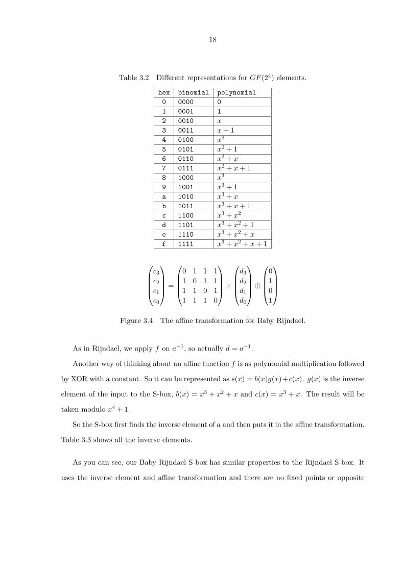
Table 3.2 Different representations for GF (24) elements. . . . . . . . . . . . . . . 18
Table 3.3 The inverse elements. . . . . . . . . . . . . . . . . . . . . . . . . . . . . 19
Table 5.1 S-box space matrix. . . . . . . . . . . . . . . . . . . . . . . . . . . . . . 33
Table 6.1 Values of ti. . . . . . . . . . . . . . . . . . . . . . . . . . . . . . . . . . 39
vii
LIST OF FIGURES
Figure 1.1 Iterative block cipher with three rounds. . . . . . . . . . . . . . . . . . 3
Figure 1.2 Key-alternating block cipher with two rounds. . . . . . . . . . . . . . . 3
Figure 2.1 The matrices A and K. . . . . . . . . . . . . . . . . . . . . . . . . . . . 7
Figure 2.2 The M matrix. . . . . . . . . . . . . . . . . . . . . . . . . . . . . . . . 8
Figure 2.3 The affine transformation. . . . . . . . . . . . . . . . . . . . . . . . . . 11
Figure 2.4 SubBytes. . . . . . . . . . . . . . . . . . . . . . . . . . . . . . . . . . . 12
Figure 2.5 ShiftRows. . . . . . . . . . . . . . . . . . . . . . . . . . . . . . . . . . . 12
Figure 2.6 MixColumns. . . . . . . . . . . . . . . . . . . . . . . . . . . . . . . . . 13
Figure 2.7 AddRoundKey. . . . . . . . . . . . . . . . . . . . . . . . . . . . . . . . 13
Figure 3.1 SubBytes operation. . . . . . . . . . . . . . . . . . . . . . . . . . . . . 16
Figure 3.2 ShiftRows operation. . . . . . . . . . . . . . . . . . . . . . . . . . . . . 16
Figure 3.3 MixColumn operation. . . . . . . . . . . . . . . . . . . . . . . . . . . . 17
Figure 3.4 The affine transformation for Baby Rijndael. . . . . . . . . . . . . . . . 18
Figure 5.1 One round of Baby Rijndael. . . . . . . . . . . . . . . . . . . . . . . . . 30
Figure 6.1 Four rounds of Baby Rijndael. . . . . . . . . . . . . . . . . . . . . . . . 35
viii
ABSTRACT
There are several recently proposed algorithms for solving the overdefined MQ problem,
two of them are XL represented in (2) and XSL represented in (3). There is an opinion that
these algorithms may be used as an attack on AES, because AES can be represented as an
overdefined MQ problem.
In our research we constructed a new cipher called Baby Rijndael. It is a scaled-down
version of Rijndael with the same algebraic structure. We apply the XL and XSL attacks on
Baby Rijndael to see if it might be possible to apply them on AES.
1
CHAPTER 1. Introduction
1.1 Ciphers
There are some very basic concepts in cryptography we should define.
Definition 1.1.1. A cryptosystem is a five-tuple (P,C, K, E, D), where:
1. P is a finite set of possible inputs/plaintexts,
2. C is a finite set of possible outputs/ciphertexts,
3. K is a finite set of possible keys, and
4. for each k ∈ K there is an encryption function ek ∈ E, and a corresponding decryption
function dk ∈ D. Each ek : P → C and dk : C → P has the property dk(ek(x)) = x for
every plaintext element x ∈ P .
The function ek is called a cipher. There are many different kinds of ciphers. All of them
take a message as an input and give back some output. The message can be represented in
many ways; it may be just an array of letters or words, or it might be text represented as
numbers, or even binary numbers. The output also can be some array of letters or numbers.
We will call the input a plaintext block and the output a ciphertext block. The operation
of transforming a plaintext block into a ciphertext block is called encryption. The operation of
transforming a ciphertext block into a plaintext block is called decryption. Most of the ciphers
use not only some input, but also a key, because it makes the cipher more secure.
Assume Alice wants to send a secret message to Bob. She wants to be sure that nobody
except Bob can read the message. This is easy to do if they have some cipher that nobody but
2
them knows or if they share some secret key. However, in many cases, Bob will never see or
speak to Alice, so they won’t be able to agree upon such a cipher or a key.
There are two different kinds of ciphers using keys: public-key ciphers and private-key
ciphers. The big difference between these two is that in a private-key cipher, only Alice and
Bob know the secret key. In public-key cipher, the key is not secret—everyone knows it. We
can define these concepts more precisely as follows.
Definition 1.1.2. A public-key cryptosystem is a cryptosystem in which each participant
has a public key and a private key. It should be infeasible to determine the private key from
knowledge of the public key. To send a message to Alice, Bob will use her public key. Nobody
except Alice knows her private key, and one must know the private key to decrypt the message.
The most well-known public key cryptosystem is the RSA cryptosystem. More detail can
be found in (8). However, in this paper we will be dealing with AES, also called Rijndael,
which is a private-key cryptosystem.
Definition 1.1.3. A symmetric-key cryptosystem (or a private-key cryptosystem) is a
cryptosystem in which the participants share a secret key. To encrypt a message, Bob will
use this key. To decrypt the message Alice will either use the same key or will derive the
decryption key from the secret key. In a symmetric-key cryptosystem, exposure of the private
key makes the system insecure.
Definition 1.1.4. A block cipher is a function which maps n-bit plaintext blocks to n-bit
ciphertext blocks. The function is parameterized by a key. n is called the block size.
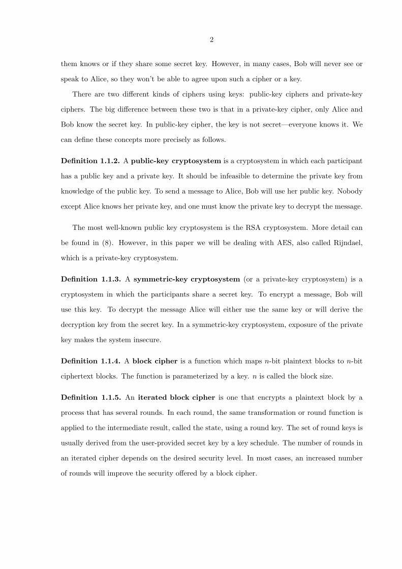
Definition 1.1.5. An iterated block cipher is one that encrypts a plaintext block by a
process that has several rounds. In each round, the same transformation or round function is
applied to the intermediate result, called the state, using a round key. The set of round keys is
usually derived from the user-provided secret key by a key schedule. The number of rounds in
an iterated cipher depends on the desired security level. In most cases, an increased number
of rounds will improve the security offered by a block cipher.
3
Figure 1.1 Iterative block cipher with three rounds. (4) pg. 25.
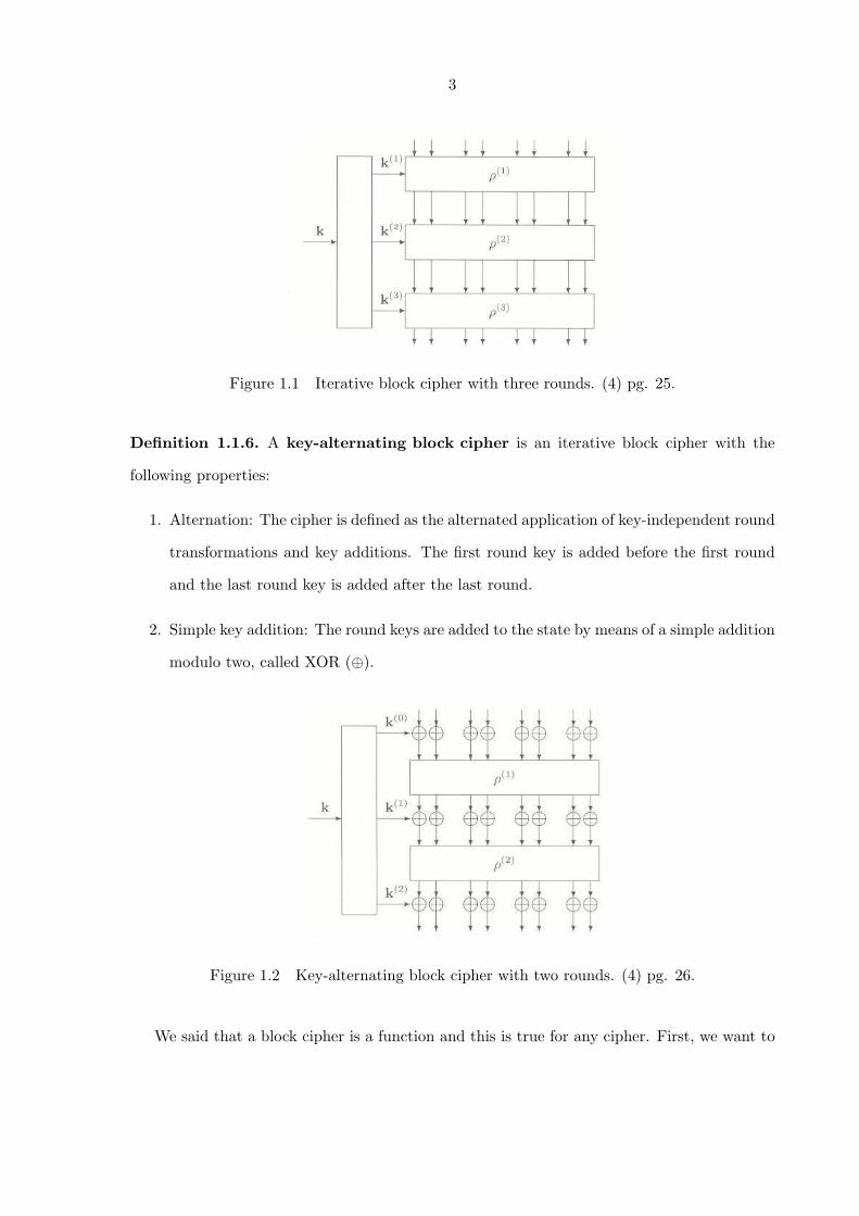
Definition 1.1.6. A key-alternating block cipher is an iterative block cipher with the
following properties:
1. Alternation: The cipher is defined as the alternated application of key-independent round
transformations and key additions. The first round key is added before the first round
and the last round key is added after the last round.
2. Simple key addition: The round keys are added to the state by means of a simple addition
modulo two, called XOR (⊕).
Figure 1.2 Key-alternating block cipher with two rounds. (4) pg. 26.
We said that a block cipher is a function and this is true for any cipher. First, we want to
4
encrypt plaintext, and then we want to decrypt ciphertext to get our plaintext back. So the
important condition for our function is to be one-to-one.
Definition 1.1.7. A function is one-to-one if no two different elements in the domain are
mapped to the same element in image.
The purpose of a cipher is to make communication secure. It is not enough to be sure that
you cannot crack the cipher you build, you should be sure that no one else can crack it either.
There are many known attacks and you should check your cipher cannot be cracked by any of
them, at least not easily.
There is one attack that can be applied to any symmetric-key cipher.
Definition 1.1.8. A brute-force attack is a known-plaintext attack. It tries every possible
key until one of them “works”. That is, knowing the input and output, the attack will try
all possible keys until it finds a key K so that the encryption of the input with K gives the
desired output.
It is easy to see why this attack will always work. The problem is that the running time of
such attack might be very large. It can sometimes take years! This is why AES can be cracked
by Brute-Force in an ideal world, but in real life, based on current technology, it can not.
We should mention that there might be more than one key. That is, if you know both the
plaintext and the ciphertext, there might be more than one key that will encrypt plaintext to
this ciphertext. Actually, the false-positive probability for a key is 1− e−2m−n, if we know one
block of size n, and the key size is m. If we know 2 blocks, then the false-positive probability
will become smaller: 1− e−2m−2n.
In our research we will build a new cipher called Baby Rijndael. We will represent it as an
MQ problem and try to attack it using MQ problem solving techniques.
1.2 MQ problem
The problem of a solving linear system of equations with n equations and n unknowns is
easy. Gaussian elimination is a well-known algorithm for solving such a system and it has a
5
running time of O(n3). Actually, depending on the system of equations, there are even quicker
techniques.
The MQ problem is a problem of solving multivariate quadratic equations. This means
that the equations we will have in our system can have quadratic terms. We will consider a
system with m equations and n unknowns with m > n, over the field GF (2).
Each equation for the MQ problem can be represented as:
∑
i,j
ai,j,kxixj +∑
i
bi,kxi + ck = 0
where xi’s are unknown, ai,j,k, bi,k, ck ∈ GF (2) are constant and k index the equations we are
looking at.
As we said before, a linear system of equations has a polynomial time running algorithm,
but the MQ problem is NP-hard problem. For references see (5). Until now, it was believed
that exponential time is needed to solve this problem.
However, for the overdefined system of multivariate quadratic equations, (that is, m > n),
more algorithms with better running time have been found. For example, Kipnis and Shamir
in (6) presented a new algorithm called relinearization. They think that for a sufficiently
overdefined system, their algorithm will run in polynomial time. For more detail see (6). After
their publication, many improved algorithms for relinearization were suggested.
The idea of all these algorithms is simple. We do not know in general how to solve the
MQ problem, but we do know how to solve a linear system of equations. So we will transfer
multivariate quadratic equations to linear equations. We will discuss this more in Chapter 4.
The problem is that it is not yet clear how these algorithms will work in real life and what
running time they will have. It has only been checked on small examples, and there might be
cases when the algorithms they present will not work.
6
CHAPTER 2. Rijndael - AES - Advanced Encryption Standard
2.1 AES
On January 2, 1997, the National Institute of Standards and Technology (NIST) began
looking for a replacement for DES — the Data Encryption Standard. DES was used an en-
cryption standard for almost 25 years. The decision was made to replace the standard because
the key length of DES was too small and some new attacks using faster new computers could
crack DES. Even a Brute-Force search is possible, because for DES, only 255 key options exist.
It was not secure anymore. The new cryptosystem would be called AES — the Advanced
Encryption Standard. It should have a block length of 128 bits and support key lengths of
128, 192 and 256 bits. Fifteen of the submitted systems met these criteria and were accepted
by NIST as candidates for AES. All of the candidaes were evaluated according to three main
criteria: security, cost (such as computational efficiency), and algorithm and implementation
characteristics (such as flexibility and algorithm simplicity). There were five finalists, all of
which appeared to be secure. On October 2, 2000, Rijndael was selected to be the Advanced
Encryption Standard, because its security, performance, efficiency, implementability and flex-
ibility were judged to be superior to the other finalists. Finally, Rijndael was adopted as a
standard on November 26, 2001, and published in the Federal Register on December 4, 2001.
There is only one difference between Rijndael and AES. Rijndael can support block and
key lengths between 128 and 256 bits which are multiples of 32. AES only has a specific block
length of 128 bits.
7
2.2 Rijndael structure
Rijndael is a key iterated and key-alternating block cipher. In this section, we will describe
Rijndael with a block size and key size of 128 bits and with 10 rounds.
The cipher has the form
E(A) = r10 ◦ r9 ◦ · · · ◦ r2 ◦ r1(A⊕K0).
Every round except the last one has the form
ri(A) = (t ◦ σ̂ ◦ S∗(A))⊕Ki,
where A is the state and Ki is the ith round key. The last round will not have the t operation.
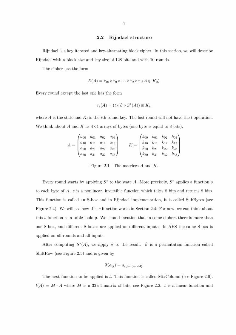
We think about A and K as 4×4 arrays of bytes (one byte is equal to 8 bits).
A =
a00 a01 a02 a03
a10 a11 a12 a13
a20 a21 a22 a23
a30 a31 a32 a33
K =
k00 k01 k02 k03
k10 k11 k12 k13
k20 k21 k22 k23
k30 k31 k32 k33
Figure 2.1 The matrices A and K.
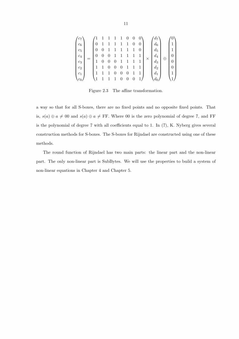
Every round starts by applying S∗ to the state A. More precisely, S∗ applies a function s
to each byte of A. s is a nonlinear, invertible function which takes 8 bits and returns 8 bits.
This function is called an S-box and in Rijndael implementation, it is called SubBytes (see
Figure 2.4). We will see how this s function works in Section 2.4. For now, we can think about
this s function as a table-lookup. We should mention that in some ciphers there is more than
one S-box, and different S-boxes are applied on different inputs. In AES the same S-box is
applied on all rounds and all inputs.
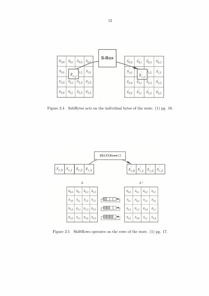
After computing S∗(A), we apply σ̂ to the result. σ̂ is a permutation function called
ShiftRow (see Figure 2.5) and is given by
σ̂(aij) = ai,j−i(mod4).
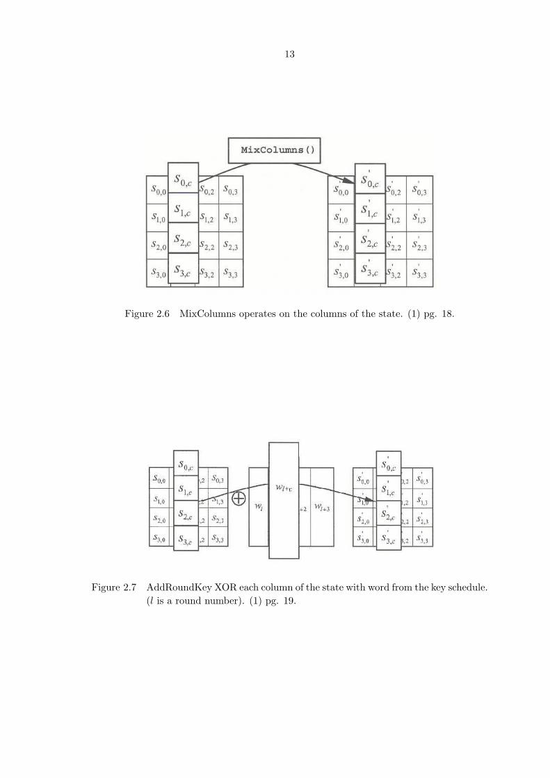
The next function to be applied is t. This function is called MixColumn (see Figure 2.6).
t(A) = M · A where M is a 32×4 matrix of bits, see Figure 2.2. t is a linear function and
8
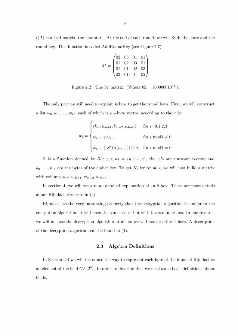
t(A) is a 4×4 matrix, the new state. At the end of each round, we will XOR the state and the
round key. This function is called AddRoundKey (see Figure 2.7).
M =
02 03 01 0101 02 03 0101 01 02 0303 01 01 02
Figure 2.2 The M matrix. (Where 02 = (00000010)T ).
The only part we still need to explain is how to get the round keys. First, we will construct
a list w0, w1, . . . , w43, each of which is a 4-byte vector, according to the rule:
wi =
(k4i, k4i+1, k4i+2, k4i+3) for i=0,1,2,3
wi−4 ⊕ wi−1 for i mod4 6= 0
wi−4 ⊕ S∗(α̂(wi−1))⊕ ci for i mod4 = 0
α̂ is a function defined by α̂(x, y, z, u) = (y, z, u, x), the ci’s are constant vectors and
k0, . . . , k15 are the bytes of the cipher key. To get Ki for round i, we will just build a matrix
with columns w4i, w4i+1, w4i+2, w4i+3.
In section 4, we will see a more detailed explanation of an S-box. There are more details
about Rijndael structure in (4).
Rijndael has the very interesting property that the decryption algorithm is similar to the
encryption algorithm. It will have the same steps, but with inverse functions. In our research
we will not use the decryption algorithm at all, so we will not describe it here. A description
of the decryption algorithm can be found in (4).
2.3 Algebra Definitions
In Section 2.4 we will introduce the way to represent each byte of the input of Rijndael as
an element of the field GF (28). In order to describe this, we need some basic definitions about
fields.
9
Definition 2.3.1. A group is an ordered pair (G, ?), where G is a set and ? is a binary
operation on G satisfying the following axioms:
1. ((a ? b) ? c) = (a ? (b ? c)), for all a, b, c ∈ G.
2. There exists an identity element e such that for all a ∈ G, a ? e = e ? a = a.
3. For each a ∈ G, there is an inverse element a−1 such that a ? a−1 = a−1 ? a = e.
Definition 2.3.2. A group is an Abelian group if for every a, b ∈ G, a ? b = b ? a.
Definition 2.3.3. A field is a set F together with the binary operations addition (+) and
multiplication (·) on F such that:
1. (F ,+) is an abelian group with identity 0.
2. (F − {0}, ·) is an abelian group.
3. For all a, b, c ∈ F , a · (b + c) = (a · b) + (a · c).
GF (28) is a field whose elements are polynomials of degree less than 8, with coefficients 0
or 1. In other words, each element of GF (28) can be written as:
a7x7 + a6x
6 + a5x5 + a4x
4 + a3x3 + a2x
2 + a1x + a0
where ai ∈ {0, 1}, for i = 0, . . . , 7.
As we can see from the definition of the field, there are two operations defined on GF (28):
addition and multiplication. Addition is performed by adding the coefficients for corresponding
powers of the polynomials modulo 2. For example,
(x7 + x5 + x4 + x2 + x) + (x6 + x5 + x3 + x2 + x + 1) = x7 + x6 + x4 + x3 + 1
Multiplication in GF (28) is performed by multiplying the two polynomials together and then
reducing this product modulo an irreducible polynomial of degree 8. For example, take irre-
ducible polynomial m(x) = x8 + x4 + x3 + x + 1, then
(x6 + x4 + x2 + x + 1) · (x7 + x + 1) = x13 + x11 + x9 + x8 + x6 + x5 + x4 + x3 + 1.
Now, take the result mod m(x):
10
x13 + x11 + x9 + x8 + x6 + x5 + x4 + x3 + 1 (modulo x8 + x4 + x3 + x + 1) ≡ x7 + x6 + 1.
Definition 2.3.4. A polynomial is said to be irreducible if it cannot be factored into nontriv-
ial polynomials over the same field. For example, over the finite field GF (23), the polynomial
x2 + x + 1 is irreducible. However, the polynomial x2 + 1 is not, because it can be written as
(x + 1)(x + 1) = x2 + 2x + 1 = x2 + 1.
There is an inverse element for every element of the field except for the 0 polynomial. The
existence of unique inverse element comes from the fact that the multiplication made modulo
an irreducible polynomial. We will think of the inverse element of 0 as 0 itself. We will use
these facts in the next chapter.
2.4 Rijndael and GF (28)
In this section, we describe how to represent a byte as an element of the finite field GF (28).
Let b7, b6, b5, b4, b3, b2, b1, b0 represent bits of a byte. Then the corresponding element of GF (28)
will be b7x7 + b6x
6 + b5x5 + b4x
4 + b3x3 + b2x
2 + b1x + b0. The addition will just be the addi-
tion defined for GF (28) and multiplication will be defined modulo the irreducible polynomial
m(x) = x8 + x4 + x3 + x + 1.
In Section 2.3, we said that an S-box is a table-lookup. However, we can actually represent
an S-box as a function s acting on elements from GF (28). Assume the input to the S-box is some
element a ∈GF (28). We can find the inverse element of a (call it a−1). This inverse element
corresponds to multiplication modulo m(x) in GF (28). If the S-box function was just defined
as an “inverse” function, then it could be attacked using algebraic manipulations. This is why
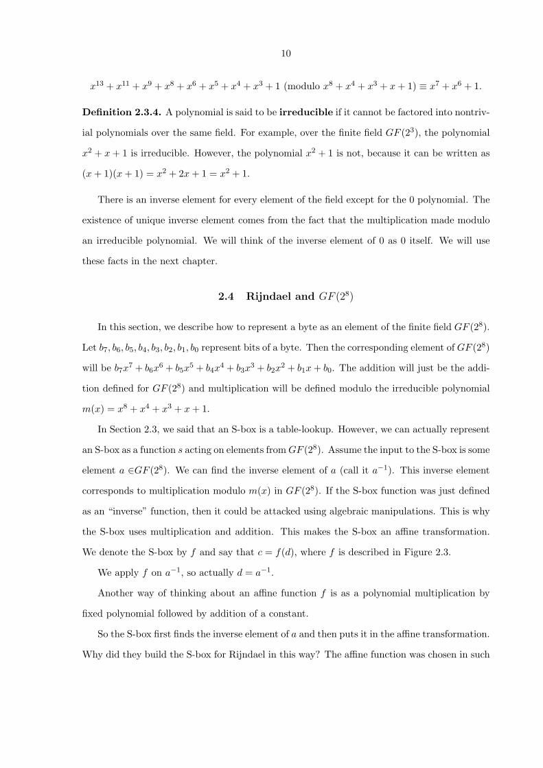
the S-box uses multiplication and addition. This makes the S-box an affine transformation.
We denote the S-box by f and say that c = f(d), where f is described in Figure 2.3.
We apply f on a−1, so actually d = a−1.
Another way of thinking about an affine function f is as a polynomial multiplication by
fixed polynomial followed by addition of a constant.
So the S-box first finds the inverse element of a and then puts it in the affine transformation.
Why did they build the S-box for Rijndael in this way? The affine function was chosen in such
11
c7
c6
c5
c4
c3
c2
c1
c0
=
1 1 1 1 1 0 0 00 1 1 1 1 1 0 00 0 1 1 1 1 1 00 0 0 1 1 1 1 11 0 0 0 1 1 1 11 1 0 0 0 1 1 11 1 1 0 0 0 1 11 1 1 1 0 0 0 1
×
d7
d6
d5
d4
d3
d2
d1
d0
⊕
01100011
Figure 2.3 The affine transformation.
a way so that for all S-boxes, there are no fixed points and no opposite fixed points. That
is, s(a) ⊕ a 6= 00 and s(a) ⊕ a 6= FF. Where 00 is the zero polynomial of degree 7, and FF
is the polynomial of degree 7 with all coefficients equal to 1. In (7), K. Nyberg gives several
construction methods for S-boxes. The S-boxes for Rijndael are constructed using one of these
methods.
The round function of Rijndael has two main parts: the linear part and the non-linear
part. The only non-linear part is SubBytes. We will use the properties to build a system of
non-linear equations in Chapter 4 and Chapter 5.
12
Figure 2.4 SubBytes acts on the individual bytes of the state. (1) pg. 16.
Figure 2.5 ShiftRows operates on the rows of the state. (1) pg. 17.
13
Figure 2.6 MixColumns operates on the columns of the state. (1) pg. 18.
Figure 2.7 AddRoundKey XOR each column of the state with word from the key schedule.(l is a round number). (1) pg. 19.
14
CHAPTER 3. Baby Rijndael
3.1 Baby Rijndael structure
3.1.1 Introduction
For the purpose of our research we constructed a new cipher called Baby Rijndael. It is a
scaled-down version of the AES cipher. Since Rijndael has an algebraic structure, it is easy
to describe this smaller cipher with a similar structure. There were many choices made when
Rijndael was constructed, so there is more than one way to build Baby Rijndael.
Baby Rijndael was constructed by Professor Clifford Bergman. He used this cipher as a
homework exercise for the cryptography graduate course at Iowa State University. He wanted
a cipher that would help his students learn how to implement Rijndael, but on a smaller, more
manageable level.
The block size and key size of baby Rijndael will be 16 bits. We will think of them as 4
hexadicimal digits (called hex digits for short), h0h1h2h3 for blocks and k0k1k2k3 for cipher
keys. Note that h0 consists of the first four bits of the input stream. However, when h0 is
considered as a hex digit, the first bit is considered the high-order bit. The same is true for
the cipher key.
For example, the input block 1000 1100 0111 0001 would be represented with h0 =8, h1 = c,
h2 = 7, h3 = 1.
Baby Rijndael consists of several rounds, all of which are identical in structure. The default
number of rounds is four, but this number is subject to change. Changing the number of rounds
affects the overall description of the cipher and also the key schedule in a small way. In our
attack, we will use both one-round Baby Rijndael and four-round Baby Rijndael.
15
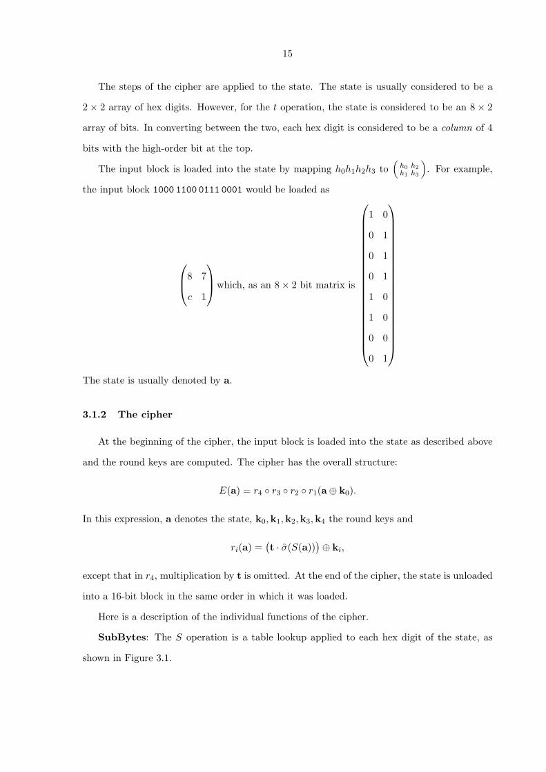
The steps of the cipher are applied to the state. The state is usually considered to be a
2× 2 array of hex digits. However, for the t operation, the state is considered to be an 8× 2
array of bits. In converting between the two, each hex digit is considered to be a column of 4
bits with the high-order bit at the top.
The input block is loaded into the state by mapping h0h1h2h3 to(
h0 h2h1 h3
). For example,
the input block 1000 1100 0111 0001 would be loaded as
8 7
c 1
which, as an 8× 2 bit matrix is
1 0
0 1
0 1
0 1
1 0
1 0
0 0
0 1
The state is usually denoted by a.
3.1.2 The cipher
At the beginning of the cipher, the input block is loaded into the state as described above
and the round keys are computed. The cipher has the overall structure:
E(a) = r4 ◦ r3 ◦ r2 ◦ r1(a⊕ k0).
In this expression, a denotes the state, k0,k1,k2,k3,k4 the round keys and
ri(a) =(t · σ̂(S(a))
)⊕ ki,
except that in r4, multiplication by t is omitted. At the end of the cipher, the state is unloaded
into a 16-bit block in the same order in which it was loaded.
Here is a description of the individual functions of the cipher.
SubBytes: The S operation is a table lookup applied to each hex digit of the state, as
shown in Figure 3.1.
16
(h0 h2
h1 h3
)S−−→
(s(h0) s(h2)s(h1) s(h3)
)
Figure 3.1 SubBytes operation.
where the s function is given by Table 3.1.
Table 3.1 S-box table lookup.
x 0 1 2 3 4 5 6 7 8 9 a b c d e fs(x) a 4 3 b 8 e 2 c 5 7 6 f 0 1 9 d
In the next section we will describe how to get this table.
ShiftRows: The σ̂ operation simply swaps the entries in the second row of the state,
Figure 3.2.
(h0 h2
h1 h3
)σ̂−−→
(h0 h2
h3 h1
)
Figure 3.2 ShiftRows operation.
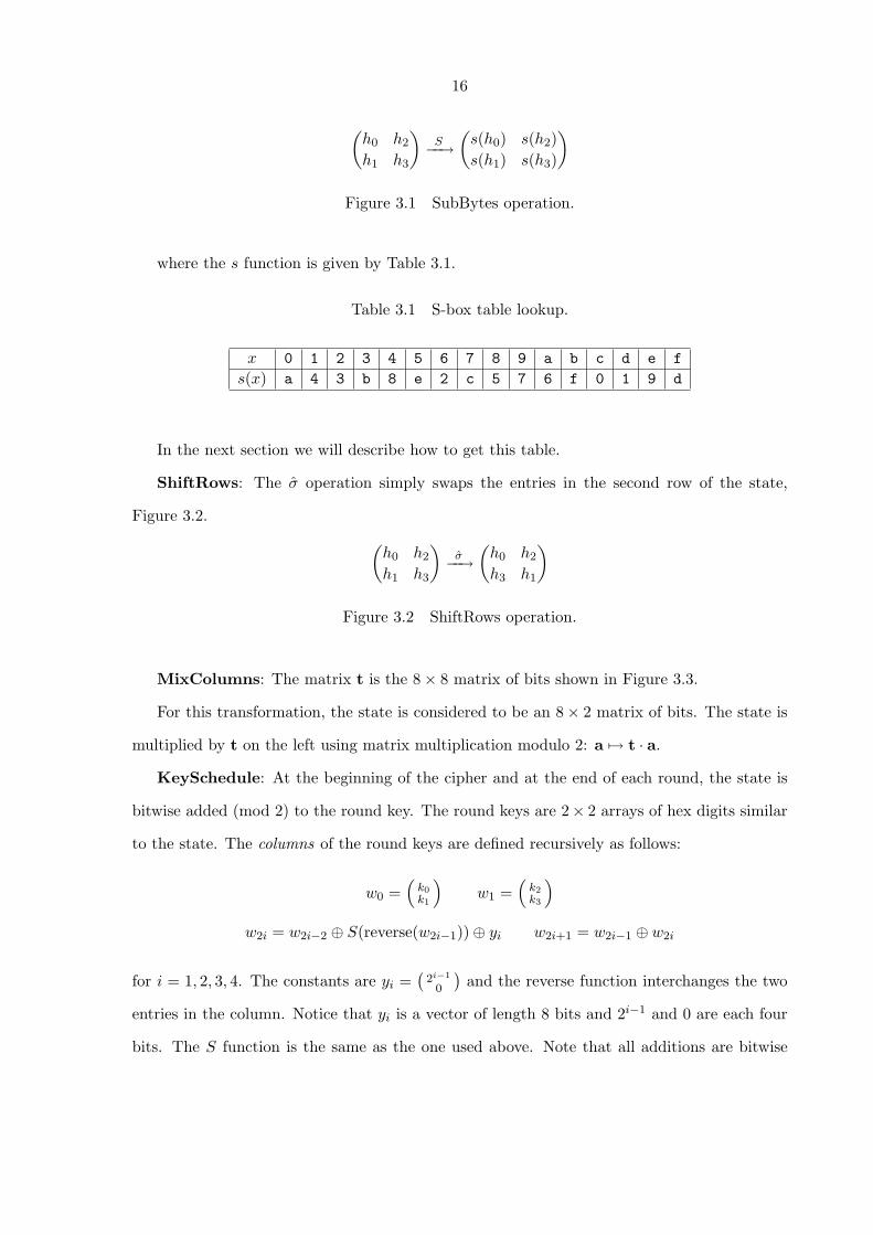
MixColumns: The matrix t is the 8× 8 matrix of bits shown in Figure 3.3.
For this transformation, the state is considered to be an 8× 2 matrix of bits. The state is
multiplied by t on the left using matrix multiplication modulo 2: a 7→ t · a.
KeySchedule: At the beginning of the cipher and at the end of each round, the state is
bitwise added (mod 2) to the round key. The round keys are 2× 2 arrays of hex digits similar
to the state. The columns of the round keys are defined recursively as follows:
w0 =(
k0k1
)w1 =
(k2k3
)
w2i = w2i−2 ⊕ S(reverse(w2i−1))⊕ yi w2i+1 = w2i−1 ⊕ w2i
for i = 1, 2, 3, 4. The constants are yi =(
2i−1
0
)and the reverse function interchanges the two
entries in the column. Notice that yi is a vector of length 8 bits and 2i−1 and 0 are each four
bits. The S function is the same as the one used above. Note that all additions are bitwise
17
t =
1 0 1 0 0 0 1 11 1 0 1 0 0 0 11 1 1 0 1 0 0 00 1 0 1 0 1 1 10 0 1 1 1 0 1 00 0 0 1 1 1 0 11 0 0 0 1 1 1 00 1 1 1 0 1 0 1
Figure 3.3 MixColumn operation.
mod 2. Finally, for i = 0, 1, 2, 3, 4, the round key ki is the matrix whose columns are w2i and
w2i+1.
Baby Rijndael has a structure similar to Rijndael. If we look at a round of Baby Rijndael,
it has the same functions as Rijndael. All the functions constructed for Baby Rijndael were
built in the same way as the Rijndael functions, but they will work on a smaller state. For
example, ShiftRows for Baby Rijndael works in the same way as ShiftRows of Rijndael works
on the 2×2 upper left submatrix of Rijndael. The KeySchedule uses the same definition as in
Rijndael, but only for 2 smaller w’s. In Section 3.2, we will see why the S-box construction of
both ciphers is similar.
3.2 Baby Rijndael S-box Structure
We described in Section 2.4 how to represent a byte as an element of finite field GF (28).
Now we will show how to represent a hex digit as an element of field GF (24). Let b =
b3, b2, b1, b0. Then the corresponding element of GF (24) will be b3x3 + b2x
2 + b1x + b0 (see
Table 3.2). The addition for GF (24) will be defined in usual way and multiplication will be
defined modulo the irreducible polynomial m(x) = x4 + x + 1.
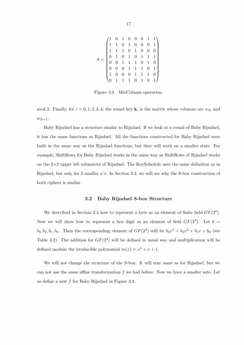
We will not change the structure of the S-box. It will stay same as for Rijndael, but we
can not use the same affine transformation f we had before. Now we have a smaller sate. Let
us define a new f for Baby Rijndael in Figure 3.4.
18
Table 3.2 Different representations for GF (24) elements.
hex binomial polynomial0 0000 01 0001 12 0010 x
3 0011 x + 14 0100 x2
5 0101 x2 + 16 0110 x2 + x
7 0111 x2 + x + 18 1000 x3
9 1001 x3 + 1a 1010 x3 + x
b 1011 x3 + x + 1c 1100 x3 + x2
d 1101 x3 + x2 + 1e 1110 x3 + x2 + x
f 1111 x3 + x2 + x + 1
c3
c2
c1
c0
=
0 1 1 11 0 1 11 1 0 11 1 1 0
×
d3
d2
d1
d0
⊕
0101
Figure 3.4 The affine transformation for Baby Rijndael.
As in Rijndael, we apply f on a−1, so actually d = a−1.
Another way of thinking about an affine function f is as polynomial multiplication followed
by XOR with a constant. So it can be represented as s(x) = b(x)g(x)+c(x). g(x) is the inverse
element of the input to the S-box, b(x) = x3 + x2 + x and c(x) = x3 + x. The result will be
taken modulo x4 + 1.
So the S-box first finds the inverse element of a and then puts it in the affine transformation.
Table 3.3 shows all the inverse elements.
As you can see, our Baby Rijndael S-box has similar properties to the Rijndael S-box. It
uses the inverse element and affine transformation and there are no fixed points or opposite
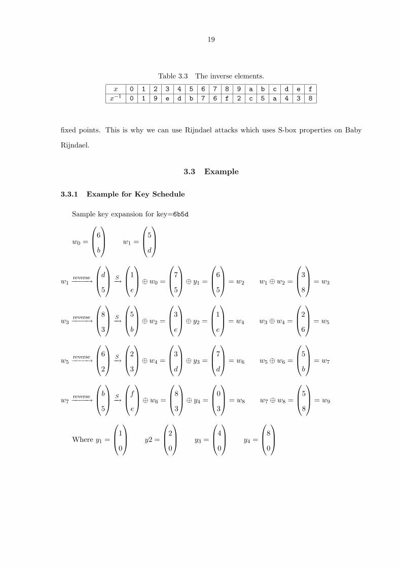
19
Table 3.3 The inverse elements.
x 0 1 2 3 4 5 6 7 8 9 a b c d e fx−1 0 1 9 e d b 7 6 f 2 c 5 a 4 3 8
fixed points. This is why we can use Rijndael attacks which uses S-box properties on Baby
Rijndael.
3.3 Example
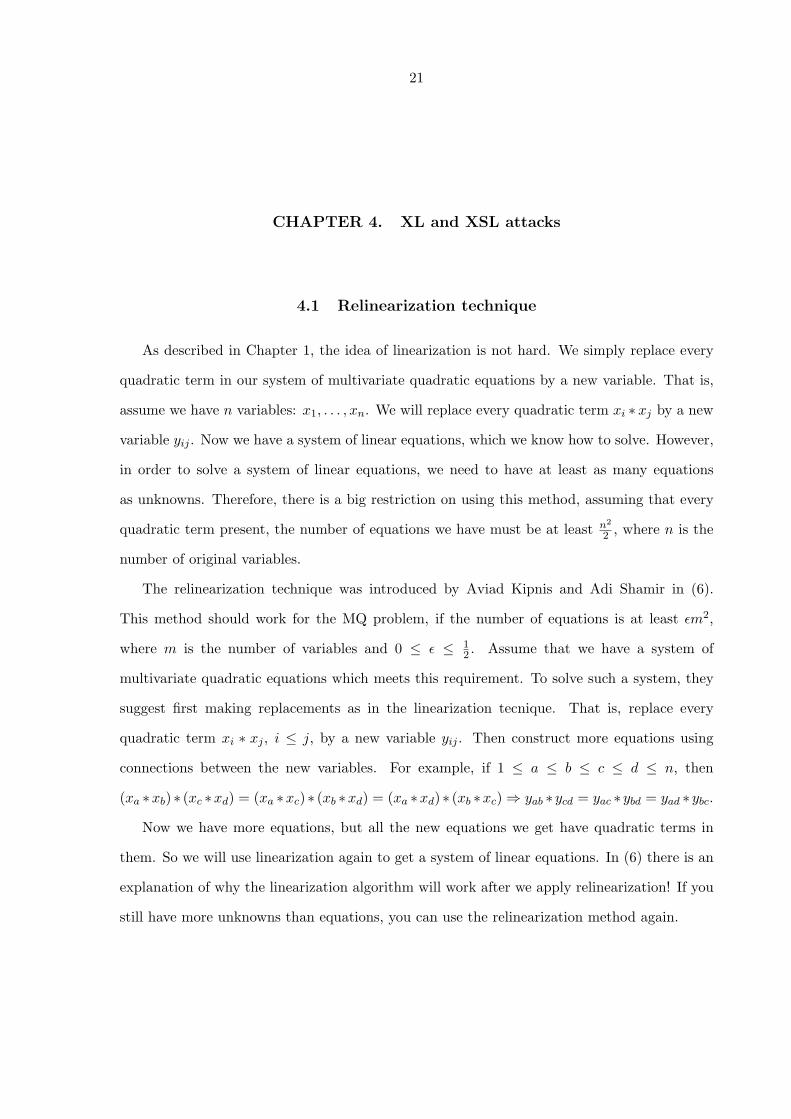
3.3.1 Example for Key Schedule
Sample key expansion for key=6b5d
w0 =
6
b
w1 =
5
d
w1reverse−−−−→
d
5
S−→
1
e
⊕ w0 =
7
5
⊕ y1 =
6
5
= w2 w1 ⊕ w2 =
3
8
= w3
w3reverse−−−−→
8
3
S−→
5
b
⊕ w2 =
3
e
⊕ y2 =
1
e
= w4 w3 ⊕ w4 =
2
6
= w5
w5reverse−−−−→
6
2
S−→
2
3
⊕ w4 =
3
d
⊕ y3 =
7
d
= w6 w5 ⊕ w6 =
5
b
= w7
w7reverse−−−−→
b
5
S−→
f
e
⊕ w6 =
8
3
⊕ y4 =
0
3
= w8 w7 ⊕ w8 =
5
8
= w9
Where y1 =
1
0
y2 =
2
0
y3 =
4
0
y4 =
8
0
20
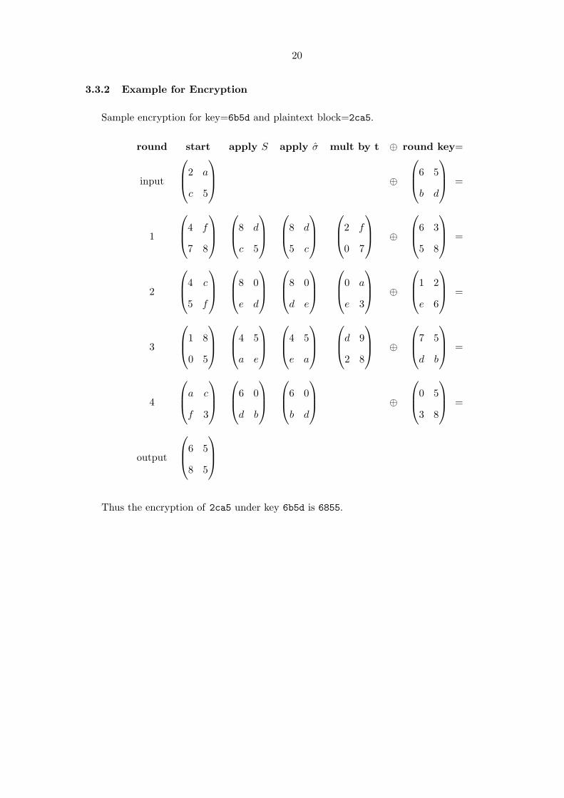
3.3.2 Example for Encryption
Sample encryption for key=6b5d and plaintext block=2ca5.
round start apply S apply σ̂ mult by t ⊕ round key=
input
2 a
c 5
⊕
6 5
b d
=
1
4 f
7 8
8 d
c 5
8 d
5 c
2 f
0 7
⊕
6 3
5 8
=
2
4 c
5 f
8 0
e d
8 0
d e
0 a
e 3
⊕
1 2
e 6
=
3
1 8
0 5
4 5
a e
4 5
e a
d 9
2 8
⊕
7 5
d b
=
4
a c
f 3
6 0
d b
6 0
b d
⊕
0 5
3 8
=
output
6 5
8 5
Thus the encryption of 2ca5 under key 6b5d is 6855.
21
CHAPTER 4. XL and XSL attacks
4.1 Relinearization technique
As described in Chapter 1, the idea of linearization is not hard. We simply replace every
quadratic term in our system of multivariate quadratic equations by a new variable. That is,
assume we have n variables: x1, . . . , xn. We will replace every quadratic term xi ∗ xj by a new
variable yij . Now we have a system of linear equations, which we know how to solve. However,
in order to solve a system of linear equations, we need to have at least as many equations
as unknowns. Therefore, there is a big restriction on using this method, assuming that every
quadratic term present, the number of equations we have must be at least n2
2 , where n is the
number of original variables.
The relinearization technique was introduced by Aviad Kipnis and Adi Shamir in (6).
This method should work for the MQ problem, if the number of equations is at least εm2,
where m is the number of variables and 0 ≤ ε ≤ 12 . Assume that we have a system of
multivariate quadratic equations which meets this requirement. To solve such a system, they
suggest first making replacements as in the linearization tecnique. That is, replace every
quadratic term xi ∗ xj , i ≤ j, by a new variable yij . Then construct more equations using
connections between the new variables. For example, if 1 ≤ a ≤ b ≤ c ≤ d ≤ n, then
(xa ∗xb)∗ (xc ∗xd) = (xa ∗xc)∗ (xb ∗xd) = (xa ∗xd)∗ (xb ∗xc) ⇒ yab ∗ ycd = yac ∗ ybd = yad ∗ ybc.
Now we have more equations, but all the new equations we get have quadratic terms in
them. So we will use linearization again to get a system of linear equations. In (6) there is an
explanation of why the linearization algorithm will work after we apply relinearization! If you
still have more unknowns than equations, you can use the relinearization method again.
22
4.2 The XL method for solving MQ problem
XL (which stands for eXtended Linearization) was created by Nicolas Courtois, Alexander
Klimov, Jacques Patarin and Adi Shamir in Eurocrypt’2000 (2). The problem they want to
solve is described in (2) in the following way:
Let K be a field, and let A be a system of multivariate quadratic equations li = 0,
(1 ≤ i ≤ m) where each li is the multivariate polynomial fi(x1, . . . , xn)− bi. The problem
is to find at least one solution x = (x1, . . . , xn) ∈ Kn, for a given b = (b1, . . . , bm) ∈ Km.
In the XL algorithm, we will need to create equations of the form (∏k
j=1 xij )∗ li = 0, where
xij ∈ (x1, . . . , xn). Equations of this type are denote by xkl, and xkl also denotes the set of all
such equations. The set of all terms of degree k is denoted by xk (so xk = {∏kj=1 xij : xij ∈
(x1, . . . , xn)}). Let D ∈ N, then ID will be the linear space generated by all the equations of
the form xkl for 0 ≤ k ≤ D − 2.
This is how they defined their algorithm.
Definition 4.2.1. The XL algorithm executes the following steps:
1. Multiply: Generate all the products (∏k
ij xij ) ∗ li ∈ ID with k ≤ D − 2.
2. Linearize: Consider each monomial in xi of degree ≤ D as a new variable and perform
Gaussian elimination on the equations obtained in 1.
The ordering on the monomials must be such that all the terms containing one variable
(say x1) are eliminated last.
3. Solve: Assume that step 2 yields at least one univariate equation in the powers of xi.
Solve this equation over the finite field K.
4. Repeat: Simplify the equations and repeat the process to find the values of the other
variables.
In other words, we will have a system of multivariate quadratic equations over the field K
23
represented as a system of equations where each equation looks like
∑
i,j
ai,j,kxixj +∑
i
bkxi + ck = 0,
where the xi’s are unknown, and k is the number of the equation.
To solve this system, we will first agree on some integer D > 2. A complexity evaluation
of XL in (2) gives the following estimation:
D ≥ n√m
,
where m is the number of equations in the original system and n is the number of variables in
the original system.
After we pick D, we will take the list of original variables and construct a new list of
variables with every possible power less or equal to D− 2. For example, if the list of variables
is (x, y, z) and D = 4, then the new list will be (x, y, z, x2, y2, z2, xy, xz, yz). Then we will
multiply each original equation by each variable from the new list. This operation will give us
more linearly independent equations. It is not necessarily true that all the new equations will
be linearly independent, but most of them will be.
Now, let’s combine the old and new systems of equations together. We will replace every
monomial we have in equations by a new variable. For example, the equation x4 + x3y +
x2yz + x2z2 + x2y = 0 will be a + b + c + d + f = 0, where a = x4, b = x3y, etc. Then we
will have a linear system of equations, with the number of equations larger than the number
of variables. This is why we should pick D carefully, so that after multiplication this condition
on the number of variables and equations will hold.
Using Gaussian elimination we can find a solution, if one exists. We still have our original
variables in the old equations, so we can get values for them. It might be that we have more
than one solution. For more examples, see (2).
The bad thing about XL is that in general, we don’t know the complexity of the algorithm.
However, for proper choices of D it seems to be more efficient than the relinearization method.
In the next chapter, we will see an example of applying this algorithm on one round of
Baby Rijndael.
24
4.3 XSL attack on MQ problem
The XL algorithm is designed for overdefined systems of quadratic equations and it seemed
to work for most of them. Some MQ problems have the property of being sparse, which means
that the equations will be missing many possible quadratic terms. People started to think
about the option of using this property to attack the system.
XSL (eXtended Sparse Linearization) was created by Nicolas Courtois and Josef Pieprzyk
in (3). The cipher was designed to crack XSL-ciphers, ciphers in which equations will be sparse.
Definition 4.3.1. An XSL-cipher is a composition of Nr similar rounds:
X The first round i = 1 starts by XORing the input with the session key Ki−1,
S Then we apply a layer of B bijective S-boxes in parallel, each on s bits,
L Then we apply a linear diffusion layer,
X Then we XOR with another session key Ki. Finally, if i = Nr we finish, otherwise we
increment i and go back to step S.
It is easy to see that AES and Baby Rijndael are both XSL-ciphers. For AES, s = 8,
B = 4 ∗ Nb, where Nb is the number of columns in the state. The number of rounds Nr
depends on the key size. For Baby Rijndael, we have Nr = 4, s = 4 and B = 4, because in
each round we apply 4 S-Boxes.
In the case of the XL attack, the authors gave the steps in the algorithm. Unfortunately,
we don’t have such a definition of XSL, because there are many steps in the algorithm that
are not clear yet even to the author. However, we do know that XSL will only work for sparse
systems of quadratic equations.
The difference between XL and XSL is that the XL attack will multiply a system of equa-
tions by every possible monomial of degree at most D−2, where D is fixed. The XSL algorithm
suggests multiplying the system of equations only by carefully selected monomials.
XSL will use the system of systems of quadratic equations built for each of the S-boxes.
For each S-box, we will have some system of equations.
First fix a constant P . More details about picking P will be given later. In every step we
25
will fix up one S-box, and call it active. All the other S-boxes will be called passive for this step.
Then we will multiply every equation of the active S-box by all products of P − 1 monomials
arising from the passive S-Boxes. We will repeat until every S-box was active exactly once.
The authors did not present a way of computing an efficient P . If P is very big, then the
attack will be similar to the XL method.
If after applying this algorithm we still do not have enough equations to use the relineariza-
tion or linearization method, Courtois and Pieprzyk in (3) suggest using the T ′ method.
After we have applied the XSL method, we will have a new system of equations. Let T
be the set of monomials we have in those equations. We still want to build more linearly
independent equations. Let Txi be the set of all the monomials from T that will still be in
T when we multiply by xi. For example, let T = {x1, x2, x3, x1 ∗ x2, x2 ∗ x3}. If we work in
GF (2), then for every x ∈ GF (2), x2 = x and Tx1 = {x1, x2, x1 ∗ x2}.Build Tx1 and Tx2 , and apply Gaussian elimination to both. We will think of every mono-
mial as a new variable, and we want to represent every variable in T −Tx1 as a combination of
variables in Tx1 and every variable in T − Tx2 as a combination of variables in Tx2 . We expect
that some subset of this resulting system will contain only terms in Tx1 , call it C1, and some
subset will contain only terms in Tx2 , call it C2. We would multiply every equation in C1 by x1.
After multiplication we will still have only terms from T in this system, so we can substitute,
and represent every term in this system as a combination of variables in Tx2 . Combine these
new equations and C2 and multiply each of the equations by x2. Now we should have some
new linearly independent equations. By iterating the process we should get more equations.
There is a toy example for the T ′ method taken from (3) given in Appendix A.
It is not clear how to choose x1 and x2, because sometimes this algorithm fails and does
not give linearly independent equations. However, the authors of the method suggest that if
one system fails, then we should pick some new variables and try the method again. They
say that most of the variables should work. More details can be found in (3). Complexity
estimates for this attack are also given in the paper.
There are two different kinds of MQ attacks on block ciphers. One of them ignores key
26
schedules, the second one uses key schedules. We should notice that the key schedule of Rijndael
uses the same S-boxes as a round of Rijndael. This is why we can build more equations using
the key schedule. The XSL attack can be applied in both MQ attacks if the block cipher we
use is an XSL-cipher.
27
CHAPTER 5. XL attack on one round of Baby Rijndael
5.1 Constructing equations
Every function can be represented as a system of equations. In this section, we will show
how to build these equations for Baby Rijndael. We will build these equations using two
different techniques. One way will use the null space equations for the S-boxes. The other way
will use the structure of the S-boxes we discussed in Section 3.2.
In this section we will use X = (x3, x2, x1, x0) to represent the input to an S-box and
Y = (y3, y2, y1, y0) to represent the output of an S-box.
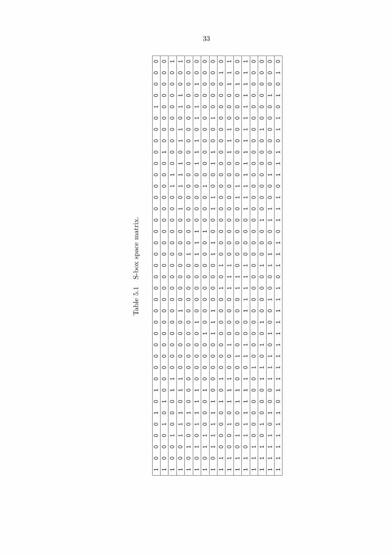
5.1.1 Null space equations
To find the null space equations, we will build a 16×37 matrix. Each row will contain the
values of 37 monomials: {1, x3, . . . , x0, y3, . . . , y0, x3x2, x3x1, . . . , x1x0, x3y3, x3y2, . . . , x0y0, y3y2,
y3y1, . . . , y1y0}, for each of 16 possible inputs of {x3, x2, x1, x0}. See Table 5.1.
After we build this matrix we can find the null space by row reduction. We use the
Mathematica function NullSpace for this. The null space will give us 21 quadratic equations.
1 + x0x1 + x0x2 + x1x2 + x0x3 + x2x3 + y0y1 + y2 + y3 = 0
x1 + x0x1 + x2 + x0x2 + x1x2 + x3 + x0x3 + x1x3 + y1 + y0y2 + y3 = 0
1 + x0 + x1 + x0x1 + x2 + x0x2 + x0x3 + y0y1 + y2 + y3 = 0
x0 + x1 + x0x1 + x2 + x0x2 + x1x2 + x3 + y1 + y2 + y3 + y0y3 = 0
x0x1 + x1x2 + x3 + x0x3 + x2x3 + y0 + y1 + y1y3 = 0
1 + x2 + x0x2 + x1x2 + x0x3 + x1x3 + y1 + y2 + y2y3 = 0
28
x0 + x1 + x0x1 + x2 + x0x2 + x1x2 + x3 + x0x3 + x0y0 + y1 + y2 + y3 + x3y3 = 0
1 + x1x2 + x3 + x0x3 + x1x3 + y0 + x0y1 + y2 + y3 = 0
x0x1 + x2 + x0x2 + x2x3 + y0 + y1 + y2 + x0y2 + y3 = 0
1 + x0 + x1 + x0x1 + x3 + x0x3 + x1x3 + y3 + x0y3 + x3y3 = 0
1 + x2 + x1x2 + x3 + x0x3 + x2x3 + y0 + x1y0 + y1 + y2 + x3y3 = 0
x0 + x1 + x0x1 + x3 + x0x3 + x2x3 + x1y1 + y2 + x3y3 = 0
x0 + x1 + x2 + x0x2 + x1x2 + x3 + x1x3 + y1 + y2 + x1y2 + y3 = 0
1 + x0x2 + x1x2 + x3 + x1x3 + y0 + y2 + y3 + x1y3 + x3y3 = 0
1 + x2 + x1x2 + x0x3 + x1x3 + x2y0 + y1 + y2 + x3y3 = 0
1 + x1 + x0x1 + x1x2 + x1x3 + x2x3 + x2y1 + y2 + y3 = 0
x1 + x0x2 + x1x2 + x3 + x2x3 + y0 + x2y2 + x3y3 = 0
1 + x0 + x1 + x0x1 + x1x2 + x1x3 + x2x3 + y0 + y1 + x2y3 + x3y3 = 0
1 + x2 + x1x2 + x3 + x0x3 + x2x3 + x3y0 + y1 + y2 = 0
x0x1 + x2 + x0x2 + x3 + x1x3 + y0 + y1 + x3y1 + y3 + x3y3 = 0
x1 + x0x1 + x2 + x0x2 + x1x2 + x3 + x0x3 + y1 + x3y2 + y3 + x3y3 = 0
This yields to 21 equations for each S-box. For one round of Baby Rijndael we will have six
S-boxes: four S-boxes in the round and another two S-boxes in the Key Schedule. This means
that we will get 21*6=126 equations. How many unknowns will we have? Each S-box has 4
input bits and 4 output bits, so we will have 8*6=48 simple variables. In addition to these null
space equations, we also have plaintext/ciphertext pair we can use. We also know something
about the structure of Baby Rijndael, so we can reduce the number of variables that we have.
We will do it in Section 5.1.3.
5.1.2 Equations with inverse property
As we showed before, an S-box of Baby Rijndael first finds the inverse element of the
input and then uses affine transformations. Let X = (x3, x2, x1, x0) be the input to S-box and
29
let Y = (y3, y2, y1, y0) be the output of the S-box. The affine transformation is a one-to-one
function, so there exists an inverse function, call it h. By applying this inverse function to Y , we
will get the inverse element of X. Therefore, we have h(Y ) = X−1, or X ∗ h(Y ) = (0, 0, 0, 1).
We can write four equations based on this relationship by equating each of the bits on the
lefthand side with a bit on the righthand side.
The equations we get are:
x0 + x2 + x3 + x0y0 + x1y0 + x2y0+
+ x3y0 + x0y1 + x1y1 + x0y2 + x2y2 + x1y3 + x2y3 + x3y3 = 0
x1 + x2 + x3 + x0y0 + x1y0 + x2y0+
+ x0y1 + x1y2 + x3y2 + x0y3 + x1y3 + x2y3 + x3y3 = 0
x0 + x1 + x2 + x3 + x0y0 + x1y0+
+ x3y1 + x0y2 + x2y2 + x3y2 + x0y3 + x1y3 + x2y3 = 0
x1 + x3 + x1y0 + x2y0 + x3y0 + x0y1+
+ x1y1 + x2y1 + x0y2 + x1y2 + x3y2 + x0y3 + x2y3 + x3y3 = 1
We have a problem if X = 0, because then X ∗ h(Y ) = (0, 0, 0, 0). This means that our
last equation is incorrect, the righthand side should be 0 instead of 1. However, we can still
use three equations.
In our attack we will use all four equations for each S-box, because for one round it is not
likely that X = (0, 0, 0, 0). If we find out that there is no solution for our system of equations,
we will erase the “bad” equations from our system and recompute it. We will do the same if
the solution we found is wrong; that is, if the solution does not propertly encrypt the given
plaintext to the ciphertext. We always can check if the key we found is the correct one by
encrypting the plaintext with this key and checking that we get the same ciphertext we have.
For each S-box we will build four equations, so we have another 4*6=24 equations (for
total of 150 equations) and still 8*6=48 variables. We will reduce the number of unknowns in
the next section.
30
For our convenience, we will rewrite the last equation in the form:
x1 + x3 + x1y0 + x2y0 + x3y0 + x0y1 + x1y1+
+ x2y1 + x0y2 + x1y2 + x3y2 + x0y3 + x2y3 + x3y3 + 1 = 0
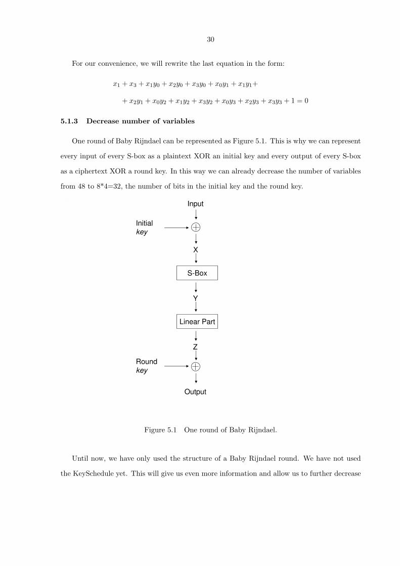
5.1.3 Decrease number of variables
One round of Baby Rijndael can be represented as Figure 5.1. This is why we can represent
every input of every S-box as a plaintext XOR an initial key and every output of every S-box
as a ciphertext XOR a round key. In this way we can already decrease the number of variables
from 48 to 8*4=32, the number of bits in the initial key and the round key.
Output
Round
key
Input
Initial
key
X
S-Box
Y
Linear Part
Z
Figure 5.1 One round of Baby Rijndael.
Until now, we have only used the structure of a Baby Rijndael round. We have not used
the KeySchedule yet. This will give us even more information and allow us to further decrease
31
the number of unknowns. Let K =
k0 k2
k1 k3
. If we will go back to Section 3.1.2, then we
will see that w3 = w1 ⊕ w2. This means that the second column of the round key is the XOR
of the second column of the initial key and the first column of the round key. In this way we
can get rid of 8 more variables, leaving us with only 24 variables.
In the next section, we will solve the system of 150 quadratic equations with 24 variables
using the XL attack.
5.2 Applying XL attack on equations
In the last section, we ended up with m = 150 quadratic equations and n = 24 simple
variables. We want to solve this system in order to find the secret key. We can’t use lineariza-
tion methods because n2 = 576 and m � n2
2 , so we need more equations. We will get these
equations by applying the XL attack.
Let’s denote the system of equations we have by S. The XL method uses a constant integer
D ≥ n√m
= 24√150
≈ 1.96. We want D to be as small as possible, because D will be the degree of
the new system, but D must be larger than two, otherwise we will stay with the same system,
so we take D = 3. This means that we should multiply every equation in S by every original
variable, because D − 2 = 1.
After this multiplication we get 150*24=3600 equation plus the original 150 equations, so
we have a total of 3750 equations with at most ( 243 ) + ( 24
2 ) + 24 = 2324 monomials. This
calculates every possible cubic, quadratic or single term. Now we can use the linearization
method. We will replace every monomial by a new variable, but we will not rename the
original variables. For example, each xixjxk = aijk, xixj = aij and if we have in some equation
just xi it will remain xi.
Remember that we are in the field GF (2). This means we have some “rules” that are not
true in general, but are true in this field. For example, x2 = x, x3 = x, 2x = 0, 3x = x, etc. We
will apply this rules to make our system easier to solve.
The idea was to use the Solve command in Mathematica to solve this linear system of
32
equations, but it did not work out. It took a lot of time and then gave an error message or ran
out of RAM. Then we built a 3750×2325 matrix. Each of the first 2324 columns will represent
a variable we might have in our system of equations and the last column will represent the
constant term. Each row is an equation from our system. To solve the system of equations, we
used Mathematica to find the Row Reduced Form of this matrix. It took less than one minute
to reduce the matrix.
The matrix in Row Reduced Form had a rank of 2292. This means that we have more than
one solution. We actually found four different solutions using the equations. We checked all of
them using the plaintext and ciphertext that we had. All four solutions we found encrypted
the plaintext we have to the ciphertext we have. So in our case the attack worked pretty well.
33
Tab
le5.
1S-
box
spac
em
atri
x.
10
00
01
01
00
00
00
00
00
00
00
00
00
00
00
00
10
00
01
00
01
01
00
00
00
00
00
00
00
00
00
00
01
00
00
00
00
10
01
00
01
10
00
00
00
00
00
00
00
01
10
00
00
00
00
11
00
11
10
11
00
00
01
00
00
00
00
10
11
10
11
01
10
01
10
10
01
00
00
00
00
00
00
01
00
00
00
00
00
00
00
00
01
01
01
11
10
00
00
10
00
00
11
10
00
00
11
10
11
01
00
10
11
00
01
00
00
10
00
00
00
01
00
01
00
00
00
00
00
01
01
11
11
00
00
01
11
00
00
11
00
11
00
11
00
10
00
00
11
00
00
10
10
00
00
00
10
10
00
00
00
00
00
00
00
01
01
10
01
01
11
00
10
00
01
11
00
00
00
00
01
11
00
01
11
11
01
00
11
00
10
00
00
11
00
00
00
11
00
00
00
00
10
01
10
11
11
11
01
10
01
11
11
00
00
11
11
11
11
11
11
11
11
10
00
00
01
00
00
00
00
00
00
00
00
00
00
00
00
00
01
11
01
00
01
10
10
10
00
01
00
01
00
00
00
01
00
00
00
11
11
01
00
11
10
10
01
00
11
00
11
00
10
00
00
01
00
01
11
11
10
11
11
11
11
11
01
11
01
11
01
11
01
10
10
10
34
CHAPTER 6. The XL and XSL attacks on four round Baby Rijnael
6.1 Equations for four round Baby Rijndael
We want to represent Baby Rijndael as an MQ problem. To do this, we will use null space
equations and properties of the S-boxes as in Chapter 5. The null space equations will stay
the same as they were in Section 5.1.1. One round of Baby Rijndael uses the same S-boxes as
four round Baby Rijndael, so again let X = (x3, x2, x1, x0) be the input to the S-box and let
Y = (y3, y2, y1, y0) be the output of the S-box. Let h be the inverse function of the affine part
of the S-box, just as in Section 5.1.2. Then X ∗ h(Y ) = (0, 0, 0, 1), unless X = (0, 0, 0, 0).
In four round Baby Rijndael, we have four S-boxes for each round and another eight S-
boxes in the Key Schedule, so we have a total of 24 S-boxes. This means that we will have
21 · 24 = 504 null space equations and another 4 · 24 = 96 equations from the inverse property.
Therefore, we have a total of 600 equations. We have four input bits to each S-box and four
output bits for each S-box, which gives 8 · 24 = 192 variables.
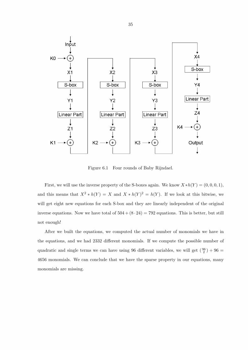
As in Section 5.1.3, we can reduce the number of variables. See Figure 6.1. We can represent
each output of an S-box as the input to the next S-box XOR with the round key. We know
the plaintext and ciphertext and we can represent the input to the first round S-box as the
plaintext XOR the initial key (K0). The output of the last round S-box will be the ciphertext
XOR the round key (K4). As in the last chapter, we have only eight (not 16) new bits for
each round key, because we can represent the other eight bits using eight bits we have and an
initial key or another round key.
In this way, we can reduce the number of original variables to 96. If we compute n2
2 we
will get 4608. We only have 600 equations, so we don’t have enough equations to use the
linearization method. We need more equations.
35
Figure 6.1 Four rounds of Baby Rijndael.
First, we will use the inverse property of the S-boxes again. We know X ∗h(Y ) = (0, 0, 0, 1),
and this means that X2 ∗ h(Y ) = X and X ∗ h(Y )2 = h(Y ). If we look at this bitwise, we
will get eight new equations for each S-box and they are linearly independent of the original
inverse equations. Now we have total of 504+ (8 · 24) = 792 equations. This is better, but still
not enough!
After we built the equations, we computed the actual number of monomials we have in
the equations, and we had 2332 different monomials. If we compute the possible number of
quadratic and single terms we can have using 96 different variables, we will get ( 962 ) + 96 =
4656 monomials. We can conclude that we have the sparse property in our equations, many
monomials are missing.
36
6.2 The XL method for four round Baby Rijndael
We have a system of n = 96 original variables and m = 792 quadratic equations. Let’s
compute the value of D we need to solve such a system using the XL method:
D ≥ n√m
=96√792
≈ 3.41.
Therefore, D = 4. This means we should multiply each equation of our system by each
possible single term and each possible monomial. We already computed this number in the
last section, the number is 4656. This means we will have a total of 792·4656+792 = 3, 688, 344
equations with ( 964 )+ ( 96
3 )+ ( 962 )+96 = 3, 469, 496 variables. This system should be solvable.
Unfortunately, we were unable to check it because the system was too big to be solved on our
computer.
Remember that in Section 5.1.2, we showed that the four equations we get from X ∗h(Y ) =
(0, 0, 0, 1) are true only in the case that X 6= 0, but we can not be sure that this condition
holds. Therefore, it might be better to drop the equation we get using the first bit. Then we
will have only three equations for each S-box, and it will reduce our system of equations to
792 − 24 = 768 quadratic equations. The number of variables will stay the same. The XL
method in this case will have 768 · 4656 + 768 = 3, 576, 576 equations. It is still should be
solvable, but again it was too large for the computer to solve.
The XL method does not use the sparse property of equations, but the XSL method uses
it. In the next section, we will use the XSL method to crack Baby Rijndael.
6.3 The XSL method for four round Baby Rijndael
We have a system of n = 96 original variables and m = 792 quadratic equations, but with
only 2332 monomials. For the XL method, we had the parameter D; for the XSL method we
need to decide on a parameter P . Unfortunately, we don’t have a formula to compute P .
We know that P should be bigger than 1, so let’s try to take P = 2. Then the algorithm we
gave in Section 4.3 says we should multiply every equation of the fixed — active S-box by all
37
products of P − 1 monomials arising from all the other — passive S-boxes. We should repeat
this multiplication until every S-box is active exactly once.
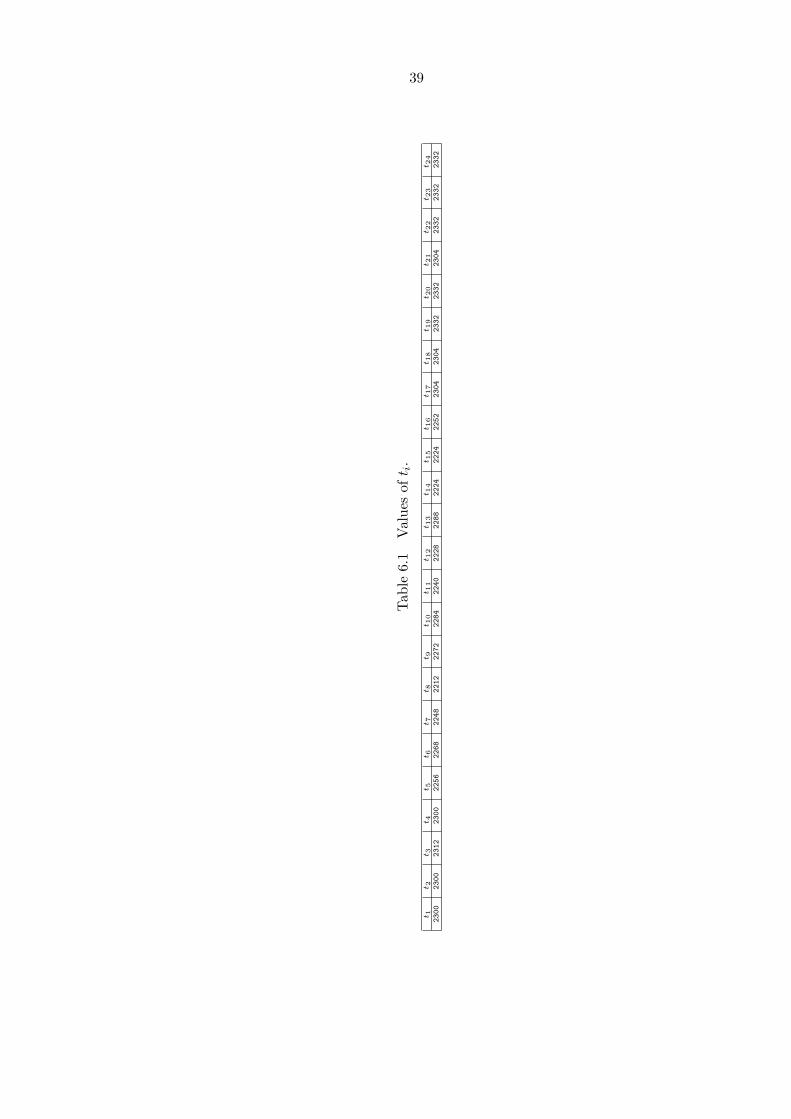
How many equations will we build and how many monomials will we have? For each S-box
we have 21 + 4 + 8 = 33 equations. Let ti be the number of monomials in the passive S-boxes
when S-box number i is active. Using Mathematica we calculated the value of these ti’s. See
Table 6.3.
We will have 1,807,740 equations. Now we should check how many monomials we have in
these equations. We can find an upper bound on the number of monomials by considering what
kind of monomials we have in our system of equations. Each monomial has degree at most four.
If we calculate all possible monomials of degree less than or equal to four of 96 variables, we
will get 3,469,496. However, we had only 2332 monomials in our original system, and then we
multiplied only by these monomials so actually we can represent it as ( 23322 )+2332 = 2, 720, 278
monomials at most. This number is smaller, but still not good enough. Using Mathematica
we found that the actual number of monomials in our system is 1,723,469. This means that
we have more equations than variables and the system should be solvable. We need to replace
every monomial by a new variable to get a linear system of equations and then we should be
able to solve this system. However, even 1,807,740 equations is too much for our computer
and we were unable to solve them.
6.4 Conclusions
From our research, we can conclude that the XL and XSL methods might work on AES.
They, at least, seemed to work on Baby Rijndael. In one round Baby Rijndael, the XL method
works for sure. For four round Baby Rijndael, we were able to construct many new equations
and get a system of linear equations with more equations than unknowns. However, we can
not be sure how many of these equations are linearly independent. We may have fewer linearly
independent equations, but we hope (and so do the authors of XL and XSL) that this method
will still work. We have a connection between the variables we don’t use in linearization
method, the new variables we constructed yij are built from the multiplication of the old
38
variables xi and xj , and yij = xixj . We can find the best solution we can from linear equations
and then try to use this connection. We could also use the relinearization method to build
more linearly independent equations, because we hope we will miss only a small number of
equations. For a sparse system of equations we can try to apply the T ′ method. As it is easy
to see from the last section, the number of monomials we have in our system is very small
compared to what it could be: we actually have 1,723,469 monomials and the upper bound
is 3,469,496 monomials. We built these new monomials using most of the same variables, so
there is a good chance we will have big enough sets T ′ and T ′′.
The XSL method seems to work better than the XL method for four round Baby Rijndael.
The number of equations we end up with in the XL method is 3,688,344 and the number of
equations for the XSL method is only 1,807,740. The number of variables we end up with for
the XL method is 3,469,496 and for the XSL this number is much smaller — only 1,723,469.
It is still not clear if the XSL method will give a better running time than a Brute Force
attack. The authors of the papers (2) and (3) think it might be better; they calculated the
estimated time for cracking AES using XSL. In our case, the Brute Force attack has a better
running time, but our initial key is much smaller than a regular Rijndael key.
It is still not clear whether XSL can break AES, but nobody has shown that it can not. In
our case, XSL seems to work, although we were unable to solve the system using our computer.
Much more research still needs to be done on the XL and XSL methods. There is disagreement
as to whether or not AES can be successfully attacked using methods to solve MQ problem.
39
Tab
le6.
1V
alue
sof
t i.
t 1t 2
t 3t 4
t 5t 6
t 7t 8
t 9t 1
0t 1
1t 1
2t 1
3t 1
4t 1
5t 1
6t 1
7t 1
8t 1
9t 2
0t 2
1t 2
2t 2
3t 2
42300
2300
2312
2300
2256
2268
2248
2212
2272
2284
2240
2228
2288
2224
2224
2252
2304
2304
2332
2332
2304
2332
2332
2332
40
APPENDIX. A Toy Example of “T ′ method”
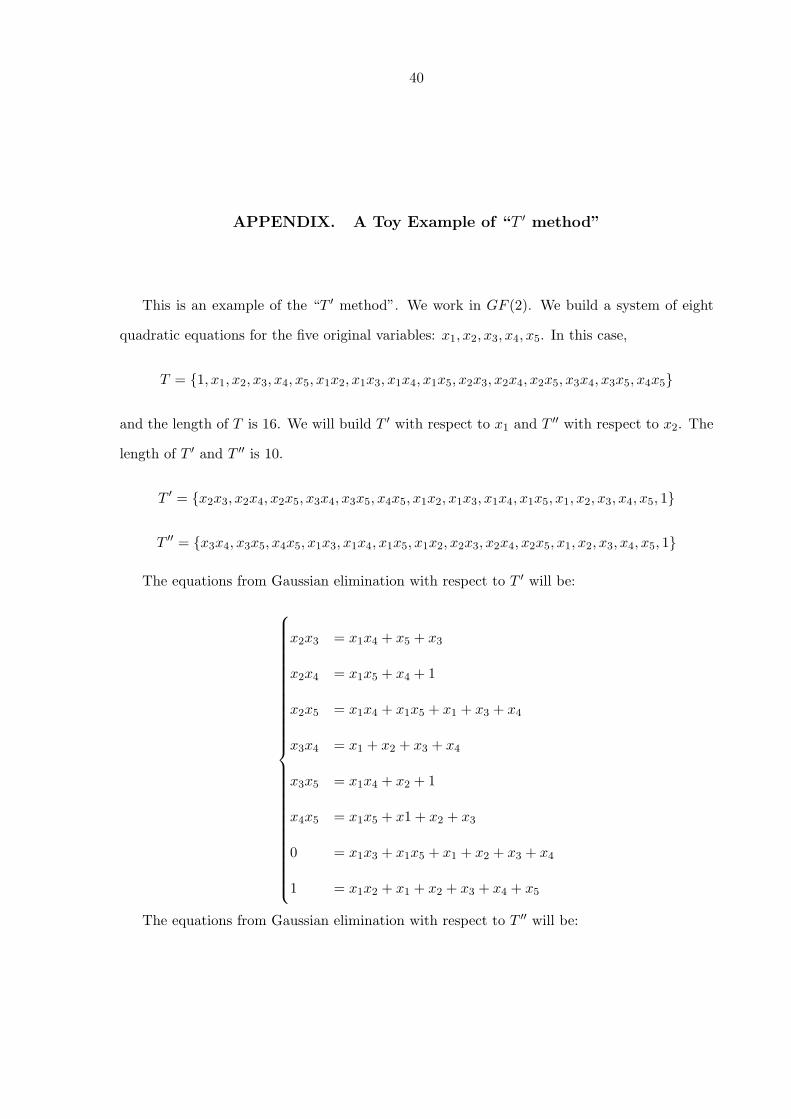
This is an example of the “T ′ method”. We work in GF (2). We build a system of eight
quadratic equations for the five original variables: x1, x2, x3, x4, x5. In this case,
T = {1, x1, x2, x3, x4, x5, x1x2, x1x3, x1x4, x1x5, x2x3, x2x4, x2x5, x3x4, x3x5, x4x5}
and the length of T is 16. We will build T ′ with respect to x1 and T ′′ with respect to x2. The
length of T ′ and T ′′ is 10.
T ′ = {x2x3, x2x4, x2x5, x3x4, x3x5, x4x5, x1x2, x1x3, x1x4, x1x5, x1, x2, x3, x4, x5, 1}
T ′′ = {x3x4, x3x5, x4x5, x1x3, x1x4, x1x5, x1x2, x2x3, x2x4, x2x5, x1, x2, x3, x4, x5, 1}
The equations from Gaussian elimination with respect to T ′ will be:
x2x3 = x1x4 + x5 + x3
x2x4 = x1x5 + x4 + 1
x2x5 = x1x4 + x1x5 + x1 + x3 + x4
x3x4 = x1 + x2 + x3 + x4
x3x5 = x1x4 + x2 + 1
x4x5 = x1x5 + x1 + x2 + x3
0 = x1x3 + x1x5 + x1 + x2 + x3 + x4
1 = x1x2 + x1 + x2 + x3 + x4 + x5
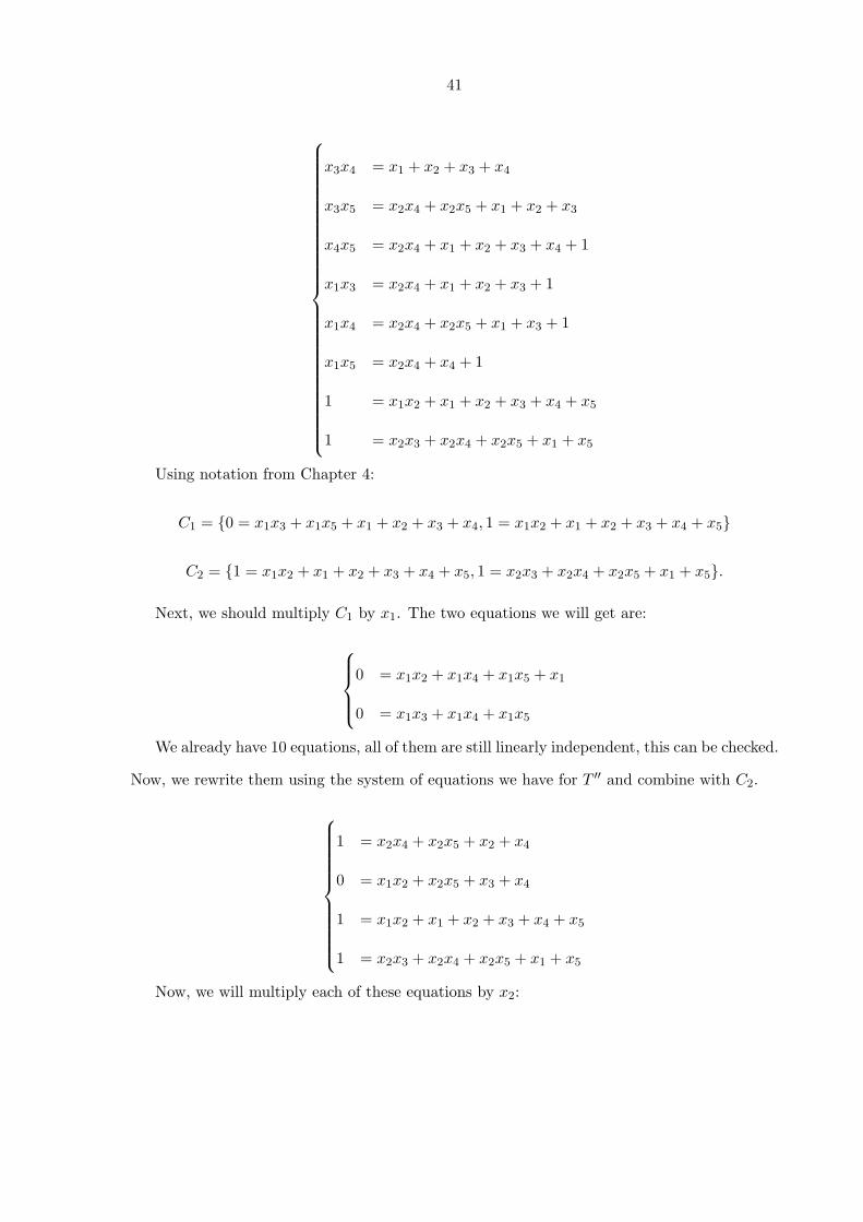
The equations from Gaussian elimination with respect to T ′′ will be:
41
x3x4 = x1 + x2 + x3 + x4
x3x5 = x2x4 + x2x5 + x1 + x2 + x3
x4x5 = x2x4 + x1 + x2 + x3 + x4 + 1
x1x3 = x2x4 + x1 + x2 + x3 + 1
x1x4 = x2x4 + x2x5 + x1 + x3 + 1
x1x5 = x2x4 + x4 + 1
1 = x1x2 + x1 + x2 + x3 + x4 + x5
1 = x2x3 + x2x4 + x2x5 + x1 + x5
Using notation from Chapter 4:
C1 = {0 = x1x3 + x1x5 + x1 + x2 + x3 + x4, 1 = x1x2 + x1 + x2 + x3 + x4 + x5}
C2 = {1 = x1x2 + x1 + x2 + x3 + x4 + x5, 1 = x2x3 + x2x4 + x2x5 + x1 + x5}.
Next, we should multiply C1 by x1. The two equations we will get are:
0 = x1x2 + x1x4 + x1x5 + x1
0 = x1x3 + x1x4 + x1x5
We already have 10 equations, all of them are still linearly independent, this can be checked.
Now, we rewrite them using the system of equations we have for T ′′ and combine with C2.
1 = x2x4 + x2x5 + x2 + x4
0 = x1x2 + x2x5 + x3 + x4
1 = x1x2 + x1 + x2 + x3 + x4 + x5
1 = x2x3 + x2x4 + x2x5 + x1 + x5
Now, we will multiply each of these equations by x2:
42
0 = x2x5
0 = x1x2 + x2x3 + x2x4 + x2x5
0 = x2x3 + x2x4 + x2x5
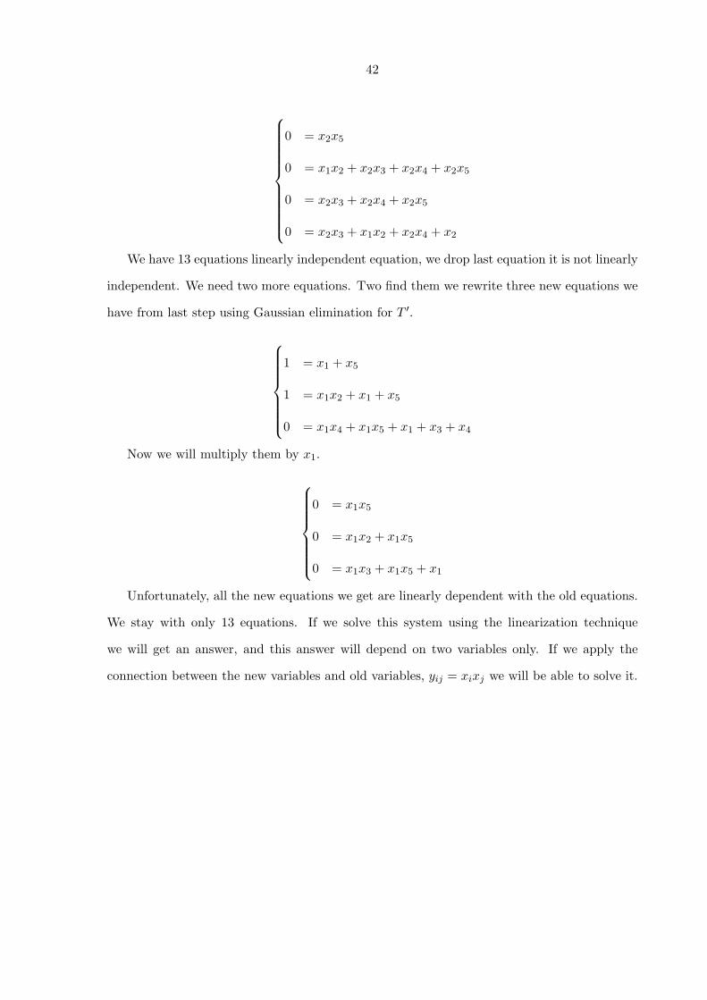
0 = x2x3 + x1x2 + x2x4 + x2
We have 13 equations linearly independent equation, we drop last equation it is not linearly
independent. We need two more equations. Two find them we rewrite three new equations we
have from last step using Gaussian elimination for T ′.
1 = x1 + x5
1 = x1x2 + x1 + x5
0 = x1x4 + x1x5 + x1 + x3 + x4
Now we will multiply them by x1.
0 = x1x5
0 = x1x2 + x1x5
0 = x1x3 + x1x5 + x1
Unfortunately, all the new equations we get are linearly dependent with the old equations.
We stay with only 13 equations. If we solve this system using the linearization technique
we will get an answer, and this answer will depend on two variables only. If we apply the
connection between the new variables and old variables, yij = xixj we will be able to solve it.
43
BIBLIOGRAPHY
[1] Advanced Encryption Standard (AES). Federal Information Processing Standards Publi-
cation 197. 2001.
[2] N. Courtois, A. Klimov, J. Patarin, A. Shamir. Efficient Algorithms for solving
Overdefined System of Multivariate Polynomial Equations. Eurocrypt’2000, LNCS 1807.
Springer-Verlag, pp. 392-407.
[3] Nicolas T. Courtois, Josef Pieprzyk. Cryptanalysis of Block Cipher with Overdefined
System of Equations. Asiacrypt 2002, Volume 2501. Springer-Verlag, pp. 267-287.
[4] Joan Daemen, Vincent Rijmen. The Design of Rijndael. Springer-Verlag, 2002.
[5] A. S. Fraenkel, Y.Yesha. Complexity of problems in games, graphs and algebraic equations.
Discrete Applied Math. Volume 1. no. 1-2. 1979. pp. 15-30.
[6] A.Kipnis, A. Shamir. Cryptanalysis of the HFE Public Key Cryptosystem by Relineariza-
tion. Crypto99, LNCS 142,144. Springer-Verlag, pp.19-31.
[7] K. Nyberg. Differentially uniform mapping for cryptography. Advances in Cryptology,
Proc. Eurocrypt’93, LNCS 765. T.Helleseth, Ed., Springer-Verlag, 1994, pp. 55-64.
[8] Douglas R. Stinson. Cryptography Theory and Practice. Second Edition. Chapman and
Hall/CRC, 2002.
44
ACKNOWLEDGEMENTS
I would like to take this opportunity to express my thanks to those who helped me with
various aspects of conducting research and the writing of this thesis. First and foremost,
Prof. Clifford Bergman for his guidance, patience and support throughout this research and
the writing of this thesis. I would also like to thank my committee members for their efforts
and contributions to this work: Prof. Giora Slutzki and Prof. Maria Axenovich. I would
additionally like to thank Kristi Meyer, Douglas Ray and Ilya Ellern for looking closely at the
thesis, correcting English style and grammar and offering suggestions for improvement.