The Wounds That Do Not Heal.

The Life-time Scar of Youth Unemployment

Gianni De Fraja

University of Nottingham & Università di Roma “Tor Vergata” & C.E.P.R.

Sara Lemos

University of Leicester

James Rockey

University of Leicester

1st February 2017

Abstract: This paper finds that unemployment shocks affect young workers for the rest

of their lives. This scar of youth unemployment is concentrated in the first few years

after entry in the labour market: one month of unemployment at age 18-20 cause a

permanent income loss of 2%. However, unemployment after that age has no long term

effect.

Keywords: Youth unemployment, Lifetime earnings, Scarring effect.

JEL-Codes: J64, J31

We would like to thank, Martin Foreaux-Koppensteiner, Andrea Ichino, Jesse Matheson, Giovanni

Pica, Till von Wachter, and seminar participants at Leicester and the ECB Labour market

conference, Frankfurt November 2014. De Fraja: gianni.defraja@nottingham.ac.uk

Lemos: sl129@leicester.ac.uk Rockey: james.rockey@leicester.ac.uk

Introduction

In many OECD countries the number of young people who are out of work is at

unprecedented levels (oecd.org/youth.htm). Substantial economic and social losses

are created by the idleness of so many otherwise productive workers. Concern about

these losses is compounded by fears about their long-term consequences. These fears

stem from the well established regularity that a person’s past unemployment is a good

predictor of their future labour market success. A seminal contribution is Ruhm’s

(1991) analysis of the long term effects of past displacement in the US, confirmed by

subsequent research, summarised in Couch and Placzeck (2010). A parallel literature

has concentrated on the long term effects of youth unemployment: Lynch (1989), or, for

the UK, Lynch (1985), Nickell et al (2002), Gregg and Tominey (2005)).1

For an adult, of course, youth is in the past, and yet the qualifiers “youth” and “past”

carry distinct connotations. This is not just a matter of semantics, but hints instead at

an important lacuna in our understanding of how past fortune shapes the causal link

between individuals’ labour market history and their current outcomes. The term “past”

emphasises how distant the shock is, whereas “youth” highlights shocks occurring in a

specific period of a person’s life, regardless of how long ago that was. This distinction,

thus, begs the question: What matters more for today’s labour market outcomes, the

timing of an unemployment shock or how far back in time it occurred?

The aim of this paper is to separate the effects of youth unemployment qua youth

unemployment from its effects as past unemployment. Our main finding is that labour

market shocks at the time of a person’s entry in the labour market are the most damaging.

The punchline of our paper is thus that wounds from youth unemployment permanently

scar, wounds from past unemployment heal. To be precise: ceteris paribus, for men, an

additional month of unemployment in the first three years after entry into the labour

market, between ages 18 and 20, permanently lowers earnings by around 2% per year.

This is a very large effect, of the same order of magnitude as the estimated decrease

in earnings attributable to the reduction of one year in formal education (Harmon et

al 2001). Furthermore, this effect shows no sign of abating by the time the individual

1Bell and Blanchflower (2011) analyse the effect of the Great Recession on young people in the the USand in the UK, while Cahuc et al (2013) consider the effect on those living in France and Germany. Also seeScarpetta et al (2010).

1

reaches 40 (see Figure 3 below). We also find that the age 18 to 20 is crucial: a similar

negative shock during the following six years, namely between ages 21 and 26, has no

long-run effects as shown again in Figure 3.

There is therefore a substantial difference in the impact of unemployment in different

sub-periods of youth: the damaging permanent effect is entirely concentrated in early

youth. This qualitative difference across years is blurred to the point of not being

recognisable when youth is treated as homogeneous period of eight years, ages 18 to 26,

as dramatically illustrated in Figure 3. Averaging across effects therefore misses the

sharp difference between subperiods within youth: for the late part of youth (ages 24 to

26), the reach of a shock is determined by distance: its effect fades as time passes.

The difference in the impact of the subperiods of youth, theoretical interest aside,

has obvious implications for the design of policies aimed at lessening the long term

effects of youth unemployment, such as the European Youth Guarantee (ILO 2012). Our

analysis suggests that putting young people into work is likely to be more effective in

the long term when precisely targeted at new entrants in the job market. It certainly

casts profound doubts on the wisdom of institutional rules which harm younger workers

for the sake of older ones.

A similar inference on the relative importance of different periods of unemployment

is reached when the overall effect is separated into its direct and indirect component: in

addition to its long term effect on earnings, a period of unemployment in youth may also

have a shorter term effect on employment, which in turn may have long term effects on

earnings. That is, being unemployed at 18 may increase the chance of being unemployed

at 22; and being unemployed at 22 may reduce a person’s future earnings. When we

separate these effects, we find that only unemployment at entry has an indirect effect.

One further and crucial dimension of variation we uncover is that individuals of different

abilities are affected differently by the scarring effect (Figure 6). Importantly, the severity

of the scar effect increases as we move down the ability scale. An unemployment shock

hitting a given cohort of young workers will be weathered more effectively, in the long

term, by high ability individuals. Therefore, such a shock exacerbates the long term

inequality in earnings among individuals of that cohort over and above any pre-existing

pre-shock inequality. Given the high level of youth unemployment in many advanced

2

economies, this suggests that further increases in inequality in those countries are likely

to occur.

For women, the negative effect of unemployment at entry in the labour market

appears to be similar (compare columns (3) and (4) in Table 1). However, in comparison

to men, the effect extends, albeit weakened, into the next three years. It also appears

to be reversed at ages 24 to 26. This might be because other confounding factors are at

play, which we cannot control for in our empirical model, as they are not available in our

dataset. One such omitted variable is hours worked per week, which is more likely to

be an important determinant of earnings for women than for men (Blundell et al 2013,

among others), given their different decisions concerning labour market participation.

This variable has also been shown to have a non-linear effect on earnings (Goldin 2014).

As a result, it is harder to disentangle the effect of youth unemployment from the effect

of other factors on earnings for females using out dataset, and, following most of the

literature, we focus our analysis on men.

We exploit a sizeable and long longitudinal dataset that has so far been largely

unused in the UK unemployment literature. The UK Lifetime Labour Market Database

combines anonymised administrative tax records and social security records into a

dataset that tracks a random sample of over 600,000 individuals between 1981 and

2006. We restrict our sample to those born between 1960 and 1967; we observe their

unemployment spells, along with their periods of employment and earnings, between the

ages of 18 and 40 (or 46 for the older individuals). This allows us to follow individuals for

an extensive period of 23 to 29 years after their entry into the labour market. Observing

unemployment spells, measured as the number of weeks unemployed within the year,

constitutes a more precise and informative measure of unemployment shocks than most

measures in the recent US literature, which are based on a binary variable measuring

“displacement” (see for example Jacobson et al 1993 and 2005, who study long term

“scarring” unemployment effects in Pennsylvania and Washington). Our dataset is also

rich in geographical detail, since it records change of address within the year. This makes

it particularly well suited to controlling for specific characteristics of the local labour

market, which affect both youth unemployment and later earnings. More crucially, we

are able to allow returns to unobserved ability to vary across local labour markets. This

3

is important since individuals might move to labour markets where their individual

skills are more valuable. Thus, an important feature of our model is that we are able to

control for endogenous geographical mobility, following Moretti’s (2004) seminal use of

detailed geographical information. Separating the effect of unemployment shocks from

the effect of unobserved individual ability, and from the effect of local labour market

characteristics, and, more crucially, from the effect of the interaction of the two, is vital

to ensure identification of the causal effect of early unemployment (and any associated

permanent effects) on earnings. Another important feature of our model is that we are

able to allow the effect of youth unemployment to vary with the time of entry in the

labour market (Figure 5). To allow for this, we follow Oreopoulos et al (2012), who studied

Canadian graduates and found that the regional conditions at the time of entry into the

labour market matter more for earnings than contemporaneous regional unemployment.

The paper is organised as follows. Section 2, which summarises the established

theoretical background on the long term effects of unemployment, motivates the

econometric specification described in Section 3. Section 4 presents the data. Our

main results and some robustness tests are in Section 5. Section 6 concludes in the light

of the existing literature.

2 The model

The theoretical model is a straightforward Mincerian equation. In its most general form,

we can write:

wti = f(Zi, λ

t, eti, εti

), (1)

where wti are person i’s earnings in period t, Zi is a vector of personal characteristics

such as years of education, innate ability, family background, and so on. λt measures

the labour market conditions in period t, given for example by the local unemployment

rates and other labour demand side variables, eti is person i’s “experience” at time t, and

εti is a random shock affecting earnings.

Early theoretical models, such as Ben-Porath’s (1967), captured experience eti as a

single figure, typically the total number of years individual i had spent in work at date

t. This reflects the idea that, when employed, a person receives both formal training

4

and “on-the-job” training.2 If information on experience is not available, “potential

experience”, given by the number of years not spent in formal education, is often used as

a proxy, as in Mincer’s landmark studies (1958 and 1974) among others.

Specifically, one can think of at least two conceptual reasons why the importance of

past events for present day outcomes depends on when these events were experienced,

necessitating a more sophisticated approach. Firstly, it is possible that recent occurrences

may matter more than distant ones: negative events fade in importance, and, conversely,

work skills acquired in the distant past become less relevant. Secondly, time may

matter because some periods in life are more important than others. It is by now

firmly established that this is the case for the formation of cognitive and non-cognitive

abilities. Heckman and his co-authors have convincingly demonstrated that people’s

early environment is substantially more important than their later environment in

determining these abilities (Cunha et al 2010). Thus, in this paper, we investigate if the

acquisition of labour market skills obeys a similar temporal pattern.

To formalise these ideas, replace eti in (1) with a vector(eti, e

t−1i , . . . , e2i , e

1i

), which

measures the experience in each of the years since the time of potential entry in the

labour market, year 1. By convention, events which occurred before year 1 are captured

by the time invariant individual characteristics term, Zi. Experience in each period is

influenced by a variety of factors, but to highlight the link between periods, we explicitly

state it as a function of past experience and the period specific random component, by

writing e2i = e2(e1i , ε

2i

), e3i = e3

(e2i , e

1i , ε

3i

), and so on. For example, the lack of experience

of “entry level” jobs caused by an early unemployment shock hinders access to jobs higher

up the jobs ladder, and, hence, reduces experience at this level. Thus (1) is replaced by:

wti = f t(Zi, λ

t, et(et−1 (. . .) , . . . , e2

(e1i , ε

2i

), e1i , ε

ti

), . . . , e2

(e1i , ε

2i

), e1i , ε

ti

). (2)

Naturally, (2) includes eti as an argument to account for the obvious direct effect of

contemporaneous events on earnings. Since experience is a “good thing”, in the sense that

increasing it should enhance earnings, we measure it so that the sign of the derivative

of wti with respect to past experience et−τi should be non-negative. The partial derivative,

2Whether generic or job specific, training enhances a person’s productivity, and, thus, future earnings.When formal training is unpaid, a further trade-off arises, as workers must choose between formal trainingand human capital accumulation while employed (Mroz and Savage 2006).

5

∂wti/∂et−τi , is the direct effect of date t− τ experience on date t earnings, whereas the

total derivative, dwti/det−τi , is its overall effect. From the latter, we can conceptually

separate a direct and an indirect effect. Taking the case t = 2 as an illustrative example,

we can write:dw2

i

de1i=∂w2

i

∂e2∂e2

∂e1i+∂w2

i

∂e1i(3)

where the total effect, dw2i /de

1i on the RHS of (3), is decomposed into the indirect effect

of period 1 experience shocks on period 2 earnings via period 2 experience and the direct

effect of period 1 experience shocks on period 2 earnings. As we explain in the next

section, our econometric strategy allows us to separate the direct from the indirect

effect. To do so is important, as the direct effect sheds light on relative importance of

the different links of the causal chain of transmission turning past shocks into present

outcomes, while the total effect measures the relative importance of shocks occurring at

different times. If∂wti∂et−τi

> 0

for some values of τ > 0 and t, then the effects of past experience are persistent: events

which occurred at time t− τ influence positively earnings at time t.

The long term importance of labour market experience is, of course well established,

and the focus of our paper is on the details of these long term effects. Some events have

only temporary effects and fade away with time. To express this hypothesis formally, we

can write ∣∣∣∣∂wti∂esi

∣∣∣∣ < δ, for t > t∗ and s = 1, . . . , s∗, (4)

for some t∗ and s∗ with t∗ > s∗ and for a suitably small value of δ. In words, (4) asserts

that if an individual is old enough (has entered the labour market at least t∗ years ago),

then early events (those that occurred in the first s∗ years after entry in the labour

market) have a “small” (less than δ) direct effect on earnings in the years more recent

than t∗. More succinctly, the effect of events experienced t− s∗ or more years ago fades

with time.

If, instead, experience gained in some years had a permanent effect on earnings, in

the way that formal education has, then (4) is replaced by the hypothesis that, for some

6

Figure 1:The partial derivatives of the earnings at time t implied by Assumption 1.

21 . . .Y

. . .A

. . . tt 1

Print as figure0.pdf \label{bar}

i

ti

e

w

S. . .

M

R. . .

s∗ and t∗ with t∗ > s∗ and M > 0,

0 < M <∂wti∂esi

, for t > t∗ and s = 1, . . . , s∗. (5)

That is, experience acquired before year s∗ has a “big” effect (larger than M ) on earnings

beyond time t∗, irrespective of the length of the period t − s∗: shocks occurring before

date s∗ leave a permanent scar.

We measure experience as the negative of unemployment, which is available in our

data for each person in each year. The idea that youth unemployment leaves permanent

“scars” but the effects of later unemployment “heals” can be cast formally in the following

hypothesis..

Assumption 1 There exist τY , τS , τA, and τR, with τY ≤ τA ≤ τS ≤ τR, and positive

constants M and δ, such that for t > τR

Scarring effect:∂wti∂eτi

> M , τ = 1, . . . , τY , (6)

Healing effect: 0 6

∣∣∣∣∂wti∂eτi

∣∣∣∣ < δ, τ = τS , . . . , τA. (7)

Where eτi < 0 is the negative of the unemployment suffered in period τ by individual

i. In words, (6) states that a shock suffered in the first τY periods has a permanent effect

on earnings, whereas according to (7), a shock suffered in periods τS to τA has a small

effect on earnings, even though periods after τS are more recent. Figure 1 illustrates

this: recent events, those happening later than τR, may have again a large impact, due

to the very fact that they are recent. Testing the hypothesis stated in Assumption 1 is

7

the aim of our empirical analysis

3 The econometric specification

If we assume equation (2) to be log-linear, and we consider earnings up to the age of 40,

then its empirical counterpart may be written as follows.3

logwti = Ztiαt + γteti︸︷︷︸

CurrentUnemployment

+ βtt−1et−1i + βtt−2e

t−2i + . . .+ βts+1e

s+1i + βtse

si︸ ︷︷ ︸

Past Unemployment Scarring Effects

, (8)

t = 19, . . . , 40, s = 18, . . . , t− 1.

Where, as in (1) and in (2), wti are the earnings of individual i in period t, Zti is a vector

of potentially time-varying individual characteristics, and −eti is the negative of the

number of weeks that individual i was unemployed in year t. In most of the papers

cited, for example in Jacobson et al (1993) and Couch and Placzek (2010), only a job loss,

a “displacement event”, is observed. Our data is much more nuanced, allowing us to

measure experience as the number of weeks of unemployment in each year. This enables

us to account for the fact that the loss of a job may affect future earnings differently

when it is followed by a long spell of unemployment, and when a new job is found after a

two week unemployment interval.

The vector of individual specific characteristics in (8), Zti , may be decomposed into

an observable component Xti , and an unobservable component V t

i . As individual charac-

teristics influence both earnings and early unemployment, unobserved heterogeneity

is a common problem with this type of model, which makes it hard to disentangle the

permanent negative effect of random unemployment shocks from the influence of an

unobserved variable, such as “ability”, or “earning potential”, on both youth employment

and future earnings. Intuitively, to the extent that employers recognise a relatively

unproductive worker, they are less likely to employ him, and because he is relatively

unproductive he also experiences lower earnings later in life. In his early contribution,

3The main regression sets 40 as the highest age; this cut-off age constitutes the best compromise betweenthe number of observations and the number of scar coefficients. As Figure 4 below illustrates, the resultsare robust to considering the full sample to age 46, when only one cohort is included in the regressionsample.

8

Ellwood (1982 p 346) remarks that this is likely to mar cross sectional studies. In

some cases, the problem is alleviated by the inclusion of a rich set of observable

individual characteristics, or by using local unemployment levels at the time of entry

as an instrument (Gregg and Tominey 2005). In this paper, our strategy is to define a

rich set of fixed effects with which to capture heterogeneity across individuals, labour

markets, time, and cohorts: a strategy made possible by the fact that we observe a large

number of individuals for well over 20 years, with detailed geographical information

for each year. The vector of fixed effects we create allows us to filter out effectively

individual, area, time and cohort characteristics and their interactions. This enables us

to identify the coefficients in the vector β.

GGGG

there are two ways of putting the fixed effects:

• as it is now:

V ti = θiµa + ηtac + εti. (9)

in the above µa takes 409 values (or indeed 819 as each can double), ηtac on the

other hand takes 65849 values = 409× 23× 7, one per cohort, per location, per year

(or 131698).

• a second possible method would be to have one counter each for cohort location

year. So we would have

V ti = θiµa + µaηcνt + εti. (10)

µa sill takes 409 values (or 819 ), ηc takes 7 one per cohort, and νt takes 23 values,

one per year. the first is better: (1) it is shorter, and (2) it has one fewer parameter

(no ν). It gets my vote also because it is clearer (to me). If James agrees, we close this

discussion, unless we get comments suggesting otherwise.

GGGG

We formally present our treatment of the fixed effects by writing the unobserved

individual characteristics as follows:

V ti = θiµa + ηtac + εti. (11)

9

The error term (11) has three components. Let time-invariant individual unobserved

determinants of earnings, such as innate ability or education, be denoted by θi. The

return to these unobserved characteristics may well vary across different labour markets.

These differences might motivate individuals to move to areas where their specific

skills are more valued. This makes location decisions endogenous. This potential

problem is analogous to that convincingly addressed by Moretti in his study of the

externalities of higher education (2004). We follow his approach by including the

interaction of the individual fixed effects θi with the area fixed effects, µa. This captures

the differences in how particular individual characteristics, including education, are

rewarded in different labour markets.4 The first term in (11) thus allows the returns to

individuals’ characteristics to vary in an unrestricted way across labour markets.

The timing of entry into the labour market is also potentially important, as shown by

Oreopoulos et al (2012) for Canadian graduates. In the second term in (11), we therefore

include cohort fixed effects. These can vary across local labour markets and across time.

We exploit the detailed geographical information in our data and interact cohort effects

with time fixed effects and with area fixed effects. Formally, ηtac, captures the shocks

affecting cohort c in the local labour market in area a in period t.

The third term in (11), εti, is the individual specific transitory component of log wages

which is allowed to be correlated with other individuals in the same cohort c entering a

given local labour market a in a given year and otherwise independent across individuals.

That is, we cluster by cohort and initial local labour market. Note that the inclusion of

the interaction fixed effects encompasses the single fixed effects: formally, θiµa includes

θi, and the triple interaction term ηtac includes the area fixed effects, the cohort fixed

effects, and the time fixed effects, as well as the “double” interaction fixed effect terms.

To sum up, our identification strategy is the following: for those who do not move,

we control for any systematic variation in labour market opportunities, with time and

cohort varying regional effects, ηtac. For those who do move, perhaps in search of local

labour markets better suited to their specific skills, this is extended with the inclusion of

a “Moretti” (2004) term, µaθi, which allows the returns to individual unobservable

4In the UK, in the period we consider, formal education is normally completed by 23 years of age. This isthe earliest that individual earnings are used in the regressions. It seems therefore reasonable to assumethat the effects of education (which we do not observe in our data) on earnings are adequately captured bythe fixed effect θi.

10

characteristics to vary across local labour markets. Formally, our identification

assumption is,

E[εtieti|θiµa, ηtac, Xit] = E[εtie

t−1i |θiµa, η

tac, Xit] = · · · = E[εtie

si |θiµa, ηtac, Xit] = 0. (12)

If we re-write (8) long-hand, to focus on the effects of the previous labour market

experience for individual i up to the age of 40, we obtain:

logw40i = X40

i α40 +γ40e40i︸ ︷︷ ︸+β4039e

39i + β4038e

38i + . . .+ β4019e

19i + β4018e

18i︸ ︷︷ ︸+V 40

i ,

logw39i = X39

i α39 +γ39e39i︸ ︷︷ ︸+β3938e

38i + . . .+ β3919e

19i + β3918e

18i︸ ︷︷ ︸+V 39

i ,

... (13)

logw20i = X20

i α20 +γ20e20i︸ ︷︷ ︸+β2019e

19i + β2018e

18i︸ ︷︷ ︸+V 20

i ,

logw19i = X19

i α19 +γ19e19i︸ ︷︷ ︸+β1918e

18i︸ ︷︷ ︸+V 19

i ,

where, as in (8), in each equation the first brace is the effect of current unemployment,

the second the effects of past unemployment spells. We can write the above system

compactly in matrix form:

logwi = αXi + γEi + βELi + Vi, (14)

where wi =(w40i , . . . , w

19i

), Xi =

(X40i , . . . , X

19i

), Ei =

(e40i , . . . , e

19i

), EL

i =(e39i , . . . , e

18i

)and Vi =

(V 40i , . . . , V 19

i

)are 22-dimensional vectors, α and γ are 22 by 22 diagonal

matrices, with(α40i , . . . , α

19i

)and

(γ40, . . . , γ19

)along the diagonal, and β is the following

upper triangular matrix:

β4039 β4038 β4037 · · · β4019 β4018

β3938 β3937 · · · β3919 β3918

β3837 · · · β3819 β3818. . . ...

...

β2019 β2018

β1918

. (15)

Writing (8) as (14) makes it clear that (8) is not identified: each equation has the

11

same number of coefficients as the number of observation per individual. To achieve

identification, we impose restrictions on the matrix β. As a first step, we consider a two

year interval for the effect of past unemployment on earnings. Formally, we set

βts = βt+1s , t = 23, 25, 27, . . . , 39. (16)

This parallels the restriction imposed by Oreopoulos et al (2012), and reduces

multicollinearity. Effectively, we study the effect on earnings measured over two years,

rather than one.

With the next set of restrictions, we concentrate on isolating the effects of

unemployment for entrants in the labour market. We split the period from age 18

to 26 into three three-year intervals. Entry into the labour market, indexed by the letter

E, age 18 to 20 inclusive; Youth, letter Y, age 21 to 23; and early Adulthood, letter A, age

24 to 26. We begin by imposing

βts = βtE , if s = 18, 19, 20 and t > 22; (17)

βts = 0, otherwise. (18)

Restriction (17) posits that a spell of unemployment at 18 is equivalent to a spell

of the same duration unemployment at 20. The coefficients βtE measure the effect

of a labour market entrant’s unemployment on their earnings from age 23 onwards.

Unemployment at ages greater than 20 is restricted in (18) not to have any long term

direct effect.

The results obtained with restrictions (17)-(18) are reported in the first column of

Table 1. When we impose these restrictions, the estimated coefficients measure the total

impact of being unemployed between ages 18 and 20. As noted earlier, however, if labour

market outcomes at a given time are influenced by past experience, then unemployment

between ages 18 and 20 harms labour market prospects at later ages: if someone is

unemployed at 19, and if experience matters for labour market prospects at 25, they

are also more likely to be unemployed at 25. As long as there is an independent effect

of unemployment at 25 on labour market outcomes at 40, this exacerbates the direct

negative effects of an entrant’s unemployment on his or her labour market outcomes at

12

40.

To disentangle the direct and indirect effect of being unemployed when young, that

is to evaluate the relative magnitude of the two terms on the RHS of (3), we modify (18)

to include additional unemployment shocks as explanatory variables. We do so in two

stages. First we add the coefficients that estimate the effects of “youth” unemployment,

defined as the years between ages 21 and 23 inclusive: thus we replace (18) with

βts = βtY , if s = 21, 22, 23 and t > 24; (19)

βts = 0, otherwise. (20)

The results obtained with restrictions (17), (19), and (20) are reported in the

second column in Table 1. Finally, we add a third possible effect, “early adulthood”

unemployment, replacing (20) with

βts = βtA, if s = 24, 25, 26 and t > 28; (21)

βts = 0, otherwise. (22)

Note that we follow Oreopoulos et al (2012) and, in (18), (20), and (22), we require

that the coefficients capturing the effects of unemployment after a certain age are 0.

Thus we disregard potential effects that are close in time to the current unemployment:

time t unemployment affects earnings at time t, whereas unemployment at time t− 1

does not. The estimated coefficients thus reflect any persistence in the unemployment

process.

To sum up, with the assumptions on the fixed effects in (11) and the restrictions on

the βs given in (17), (19), and (21)-(22), the regression specification (8) becomes:

lnwtiac = Xtiα

t + γteti + βtE

20∑s=18

esi︸ ︷︷ ︸Scarring effects

of unemployment

for Entrants

+ βtY

23∑s=21

esi︸ ︷︷ ︸Scarring effects

of unemployment

for Youths

+ βtA

26∑s=24

esi︸ ︷︷ ︸Scarring effects

of unemployment

for early Adults

+ µaθi + ηtac + εti,

t = 23-24, 25-26, . . . , 39-40. (23)

13

The coefficients βtE , βtY , and βtA measure the effects of unemployment when “Entrant”

(age 18-20), “Youth” (age 21-23) or “Early Adult” (age 24-26). The last three terms are

the error term, and are described in detail in (11).

4 The data

We use data from the Lifetime Labour Market Database (LLMDB), which combines tax

and social security records into a dataset which follows a 1% random sample of National

Insurance Number (NINo) holders, amounting to 647, 068 individuals between 1978 and

2006.5 The LLMDB is, therefore, a rich, accurate, long and broad longitudinal dataset.

It contains information on sex, and date and country of birth. For each year, it contains

information on the address of residence, earnings, nature of employment (employee or

self-employed), number of weeks of employment and unemployment in the year, and

on benefits received. Similarly to many administrative datasets, the LLMDB does not

contain information on education or family background. As they are time-invariant,

these characteristics are controlled for with the inclusion of individual fixed effects, as

explained above. Unlike Orepopolous et al (2012), we can measure employment and

unemployment at the beginning of individuals’ careers, rather than having to proxy it

with local labour averages. Given the importance of the time of entry into the labour

market to this literature, our dataset also improves on other studies, such as Gregg and

Tominey (2005), Jacobson et al (1993 and 2005) and Couch and Placzeck (2010), which

observe one cohort only.6

We restrict our sample to UK nationals, for whom we observe earnings, benefits

and employment and unemployment continuously between ages 18 to 40. The earliest

cohort in our dataset comprises individuals born in 1960, who enter the labour market in

1978. The last cohort are those born in 1966, who enter in 1984. We exclude individuals

who are recorded as ever being self-employed; these constitute 12.1% of the sample. We

5A fresh cohort of individuals enters the data every year and is followed from then on. This administrativedata is derived from a number of datasets linked by the unique individual identifier, the National Insurancenumber, which is allocated to British nationals just before they turn 16 years old and to foreign nationalswho are eligible to work and/or claim benefits.

6The LLMDB has been used in recent years to study income mobility and changes in inequality (Gardinerand Hills 1999, Dickens and McKnight 2008a), whether policy can affect the intensity of job search(Petrongolo 2009), the assimilation of immigrant workers into the UK labour market (Lemos 2013 and 2014,Dickens and McKnight 2008b), and the link between unemployment and low pay (Gosling et al 1997).

14

do so for several reasons. Firstly, income from self-employment may not be recorded

accurately. Secondly, those self-employed might have more opportunity to understate

their employment and earnings to reduce their tax liability. Thirdly, in the absence of

information on balance sheets, we are unable to distinguish an individual’s earnings

from the return on the capital that the self-employed often own (Gollin 2002). Each of

these reasons exacerbates measurement error in earnings, and in a way that is unlikely

to be orthogonal to unemployment during the individual’s youth. As a robustness check,

we run the model excluding, for individuals who have ever reported being self-employed.

Only the years when they report being self-employed. This increases the sample, whilst

making the panel unbalanced, and the results for this case are reported in column (5) of

Table 1.

The two main quantitative variables in our model are earnings and the number of

weeks of unemployment in each year. While the data for those employed are very reliable

and accurate, as is derived from the LLMDB tax records, the data for those unemployed

are derived from the LLMDB benefit records. Benefit data, in any given year, will only

capture those unemployed who meet the criteria for entitlement to a benefit. So, when it

is recorded, the record is completely accurate, as these data form the basis for benefit

payments. However, benefit data will often be missing, as it is simply not recorded for

individuals who are not in receipt of benefits. In this case, it does not necessarily imply

zero unemployment: it might mean that an individual is not entitled to benefits or that,

even when entitled, is not claiming benefits.

We base the construction of our measure of unemployment on two variables recorded

in the data: “number of employed weeks” and “number of unemployed weeks” in the

year. For just over half of the observations in our sample, the number of employed

and unemployed weeks in the year add up to 52, giving a consistent measure of

unemployment in the year. When they do not, we determine unemployment for individual

i in year t as the number of weeks individual i is recorded as unemployed. If this figure

is missing, then individual i’s unemployment in the year is defined as 52 minus the

number of weeks individual i is recorded as employed. In other words, we turn to

“employed weeks” only when “unemployed weeks” is missing, the idea being that when

“unemployed weeks” is recorded, then it is recorded accurately, because it is the measure

15

Figure 2:Yearly Earnings and Weeks of Unemployment per Year by Cohort - Men

5000

10000

15000

20000

25000

30000

Yea

rly E

arni

ngs

1978

1979

1980

1981

1982

1983

1984

1985

1986

1987

1988

1989

1990

1991

1992

1993

1994

1995

1996

1997

1998

1999

2000

2001

2002

2003

2004

2005

2006

0

2

4

6

8

Wee

ks o

f Une

mpl

oym

ent

1978

1979

1980

1981

1982

1983

1984

1985

1986

1987

1988

1989

1990

1991

1992

1993

1994

1995

1996

1997

1998

1999

2000

2001

2002

2003

2004

2005

2006

Calendar Year

Cohort 1978 Cohort 1979 Cohort 1980 Cohort 1981 Cohort 1982

Cohort 1983 Cohort 1984 Age 24 Age 40

Note: Average year earnings, measured in 2004 pounds (top panel), and average number of weeksunemployed per year (bottom panel), for men born in the various years (dark lines for individuals bornearlier), in the calendar year measured along the horizontal axis. The thick dashed lines joint the age 24points and age 40 points for each cohort.

that forms the basis on which the benefits to be paid to claimants are calculated. This

imputation is uncontroversial, and it populates the unemployment variable for over

97% of the observations in the LLMDB. Attributing a subordinate role to “employed

weeks”, which is used only when “unemployed weeks” is missing, is justified on the

grounds that the calculation of a person’s income tax liability, unlike the payment of

benefits, is independent of the recorded number of employed weeks.7 In the remaining

observations, “employed weeks” and “unemployed weeks” do not add up to 52, and we

calculate unemployment as the share of “unemployed weeks” in the sum of these two

numbers.

The final sample for our main results comprises 14348 men and 13602 women observed

for 23 years (ages 18 to 40 inclusive), a total of 645, 656 observations. Summary statistics

for our dataset are presented in Figure 2 and in Table A1 in the Appendix. These report

the cohort average rate of unemployment for each year for men entering the labour

market between 1978 and 1984, and their average gross yearly real earnings, adjusted

by the Retail Price Index and measured in 2006 pounds. The colour of the various lines

move from blue to yellow for later cohorts. We have also plotted in dashed black the line

that joins the values for each cohort at age 24 and at age 40.8

The vector Xti in (23) includes an indicator variable that takes a value of 1 if the

individual is in receipt of a benefit in the year. It also includes four indicator variables

to identify those who are structurally or long-term unemployed: the first is 1 in year t if

individual i is unemployed for all the 52 weeks of year t; the second is 1 if an individual

is unemployed for two whole years, that is for all the 104 weeks of two consecutive years.

And similarly, for three and five years. These indicator variables are meant to capture

the non-linear effects of protracted periods of structural unemployment on long-run

wages.

The last terms in (23) are the fixed effects interacted with one another, as explained

in (11). These are essential features of our econometric specification, and allow

us to separate the effects of unemployment shocks from the influence of individual

7And indeed the two measures come from data collect by two different government departments, theDepartment for Work and Pensions, and the Inland Revenue, now renamed HMRC, for different purposes,pensions and benefits, and income tax, respectively.

8The summary statistics reported in Figure 2 and Table A1 are adjusted to make them comparableover time, given changes in the underlying administrative processes generating the data. Our regressionestimates use the unadjusted data and control for these differences using fixed effects.

17

characteristics, the conditions of the local labour market where individuals find

themselves or move to, and the difference of the effects of the business cycle on different

areas of the country. We use the administrative division of the country into 409 “local

authority districts” to define area fixed effects, indexed by a.9

The information on individual addresses is complete from 1997 onwards. Prior to

this, it is missing for 36% of the observations. Given that our identification strategy is

based on the local authority district where each individual resides, care must be taken

in dealing with missing addresses. While most moves in the UK are within a short

distance and therefore subsequent local areas of residence are good predictors of previous

ones, some people will have moved further and these individuals may be systematically

different, potentially those whose labour market skills are more specialised. To account

for this difference, we introduce an artificial second set of area fixed effects: the inferred

area fixed effects are denoted by a0 ∈ {1, . . . , 409}. Individual i’s location in year t is

given by a if he is recorded as living in area a in year t; it is given by a0 if his address is

missing and his next recorded address is a, t = 23, . . . , 40. This assumption is a mid-point

between the “naïve” alternatives of treating subsequent addresses as having correlation

1 or 0 with previous ones. In the former case we would impute a single “notional-national”

address to observations where the information on location is missing.10 The results for

this treatment of missing observations are reported in Column (6) of Table 1. If instead

we believed that current address had perfect predictive power of previous addresses we

would not distinguish between a and a0, implicitly assuming that the labour market

consequences of individuals’ moves are on average zero. The results for this case are

reported in Column (7), of Table 1. These extremes can be seen as upper and lower

bounds containing the true estimate, and comparisons between columns (3), (6) and (7)

in Table 1 suggest that our results do not depend on our treatment of missing address

observations.9A full list of local authority districts is available at data.gov.uk/dataset/

local-authority-districts-uk-2012-names-and-codes. We use these, instead of “travel towork areas” (TTWAs), which are not defined consistently for our entire sample period and have beenidentified as problematic, especially prior to recent revisions (Coombes and Openshaw 1982). They are alsolarger and hence identify location less accurately.

10We could also drop all observation with a missing address: this is an inferior option, as it wouldreduce the sample, make the panel unbalanced, and omit an individual’s observations in a way likely to becorrelated to that individual employment record.

18

5 Results

The results from our preferred specification are reported in Table 1: as we explained, the

regression in (23) is estimated for the subset of the individuals who are in the sample

continuously from age 18 to 40, and it is pooled across cohorts. All coefficients are

multiplied by −100, to measure the “scar” effect in percentage terms.

The first coefficient in each column of Table 1 shows the effect of current

unemployment on current earnings: being unemployed for an additional week at age

40, other things equal, brings about a reduction in earnings at age 40 of approximately

2.3%, for men and 2% for women, numbers which are very close to 152 , the proportionate

earnings loss of a week of employment. We take this correspondence as a strong

suggestion that our specification does capture all the other individual characteristics

that may be determining earnings.

The rest of the table gives the long term effect of unemployment on current earnings.

In the first column we report, for men, solely the effect of “unemployment as Entrant”.

That is, with restrictions (17)-(18), which impose the restrictions βtY = βtA = 0 in (23).

If a man is unemployed for an additional week between ages 18 and 20, his earnings

during two year intervals between ages 23 and 40 are lowered by the percentage amount

in the corresponding row of the table. Thus, for example, the coefficient “On earnings

aged 35-36” says that one additional week unemployment suffered between ages 18 and

20 (inclusive) decreases annual earnings received between ages 35 and 36 (inclusive)

by 0.54%. Similarly, the rows in the second column, labelled “Youth”, report coefficients

measuring the effect of an additional week of unemployment between ages 21 and 23:

(19)-(20) replace (18), that is βtY is unrestricted in (23). The third column adds the period

of “Early adulthood”, ages between 24 and 26. The fourth column is the specification of

column 3 for the women in the sample.

We see a strong direct effect of unemployment at entry (age 18-20) on lifetime

earnings, in this table up to the age of 40, although when we consider a longer time

frame there is no indication that this effect is dampened (Figure 4). Columns (2) and

(3) add first unemployment between ages 21 and 23, and then between 24 and 26. The

similarity between the coefficients in the first block in the first three columns is due to

the lack of statistical significance of the coefficients in the second and third block. This

19

Table 1: Long term effects of early unemployment

Entrant Entrant& Youth

WholePeriod

Women Self-Employed

NationalAddress

FirstAddress

(1) (2) (3) (4) (5) (6) (7)

Current Unemployment 2.312∗∗∗ 2.321∗∗∗ 2.318∗∗∗ 1.949∗∗∗ 2.262∗∗∗ 2.423∗∗∗ 2.291∗∗∗

(0.051) (0.051) (0.051) (0.035) (0.046) (0.047) (0.044)Entrant Unemployment (18-20)On Earnings Aged 23-24 0.320∗∗∗ 0.321∗∗∗ 0.321∗∗∗ 0.562∗∗∗ 0.334∗∗∗ 0.383∗∗∗ 0.340∗∗∗

(0.040) (0.040) (0.040) (0.041) (0.038) (0.031) (0.031)On Earnings Aged 25-26 0.439∗∗∗ 0.447∗∗∗ 0.447∗∗∗ 0.621∗∗∗ 0.442∗∗∗ 0.534∗∗∗ 0.468∗∗∗

(0.041) (0.051) (0.051) (0.051) (0.046) (0.039) (0.042)On Earnings Aged 27-28 0.511∗∗∗ 0.537∗∗∗ 0.537∗∗∗ 0.662∗∗∗ 0.510∗∗∗ 0.607∗∗∗ 0.537∗∗∗

(0.042) (0.052) (0.052) (0.051) (0.048) (0.039) (0.044)On Earnings Aged 29-30 0.607∗∗∗ 0.570∗∗∗ 0.566∗∗∗ 0.633∗∗∗ 0.546∗∗∗ 0.641∗∗∗ 0.582∗∗∗

(0.045) (0.054) (0.054) (0.055) (0.050) (0.040) (0.046)On Earnings Aged 31-32 0.602∗∗∗ 0.553∗∗∗ 0.552∗∗∗ 0.607∗∗∗ 0.525∗∗∗ 0.634∗∗∗ 0.548∗∗∗

(0.044) (0.053) (0.053) (0.059) (0.050) (0.041) (0.047)On Earnings Aged 29-30 0.550∗∗∗ 0.498∗∗∗ 0.498∗∗∗ 0.604∗∗∗ 0.499∗∗∗ 0.602∗∗∗ 0.496∗∗∗

(0.044) (0.053) (0.053) (0.059) (0.050) (0.041) (0.046)On Earnings Aged 35-36 0.542∗∗∗ 0.491∗∗∗ 0.492∗∗∗ 0.541∗∗∗ 0.502∗∗∗ 0.580∗∗∗ 0.494∗∗∗

(0.046) (0.055) (0.055) (0.063) (0.052) (0.042) (0.048)On Earnings Aged 37-38 0.526∗∗∗ 0.487∗∗∗ 0.492∗∗∗ 0.512∗∗∗ 0.500∗∗∗ 0.568∗∗∗ 0.494∗∗∗

(0.047) (0.056) (0.056) (0.062) (0.052) (0.041) (0.049)On Earnings Aged 39-40 0.510∗∗∗ 0.500∗∗∗ 0.506∗∗∗ 0.488∗∗∗ 0.518∗∗∗ 0.587∗∗∗ 0.509∗∗∗

(0.046) (0.057) (0.056) (0.062) (0.052) (0.043) (0.050)Youth Unemployment (21-23)On Earnings Aged 25-26 −0.013 −0.013 0.056 −0.010 −0.029 −0.046

(0.045) (0.045) (0.048) (0.041) (0.033) (0.037)On Earnings Aged 27-28 −0.047 −0.047 0.061 −0.033 −0.015 −0.064

(0.046) (0.046) (0.052) (0.044) (0.034) (0.040)On Earnings Aged 29-30 0.073 0.042 0.179∗∗∗ 0.033 0.081∗ 0.003

(0.048) (0.053) (0.053) (0.050) (0.039) (0.047)On Earnings Aged 31-32 0.096 0.091 0.151∗∗ 0.086 0.116∗∗ 0.084

(0.050) (0.055) (0.058) (0.051) (0.040) (0.049)On Earnings Aged 29-30 0.100∗ 0.091 0.121∗ 0.076 0.099∗ 0.069

(0.051) (0.055) (0.060) (0.051) (0.040) (0.049)On Earnings Aged 35-36 0.100 0.098 0.143∗ 0.082 0.115∗∗ 0.075

(0.052) (0.056) (0.062) (0.052) (0.041) (0.050)On Earnings Aged 37-38 0.077 0.110 0.178∗∗ 0.078 0.145∗∗∗ 0.089

(0.052) (0.056) (0.064) (0.053) (0.040) (0.051)On Earnings Aged 39-40 0.024 0.067 0.200∗∗ 0.040 0.104∗ 0.045

(0.053) (0.057) (0.064) (0.054) (0.041) (0.052)Early Adulthood Unemployment(24-26)

On Earnings Aged 29-30 0.060 −0.137∗∗ 0.051 0.043 0.057(0.047) (0.042) (0.043) (0.037) (0.043)

On Earnings Aged 31-32 0.007 −0.141∗∗ 0.005 −0.001 0.011(0.046) (0.046) (0.044) (0.035) (0.042)

On Earnings Aged 29-30 0.016 −0.158∗∗∗ 0.009 0.013 0.019(0.049) (0.047) (0.046) (0.038) (0.046)

On Earnings Aged 35-36 0.000 −0.206∗∗∗ −0.020 0.023 0.005(0.050) (0.050) (0.046) (0.037) (0.046)

On Earnings Aged 37-38 −0.070 −0.259∗∗∗ −0.089 −0.057 −0.069(0.051) (0.050) (0.048) (0.037) (0.047)

On Earnings Aged 39-40 −0.092 −0.275∗∗∗ −0.114∗ −0.073∗ −0.092(0.051) (0.051) (0.048) (0.037) (0.048)

N 319481 319481 319481 302328 358864 319481 319481Number of Individuals 14348 14348 14348 13602 16082 14348 14348

* p < 0.05, ** p < 0.01, *** p < 0.001. The dependent variable is the (log of) total annual earnings. Estimationusing felsdvreg (Cornelissen 2008). Standard errors are clustered by ηac, i.e. cohorts defined by initial local areaand are below the associated coefficients. Reported coefficients are obtained using the estimator described in (23)and measure the percentage effect of an increased week of unemployment in the three age brackets, 18-20, 21-23,and 24-26, on earnings in different subsequent periods. All specifications also include dummy variables recordingthe receipt of benefits and long-term unemployment in during a year, as well as individual, local labour market,cohort, and time fixed effects and their interactions as explained in the discussion of (11). Columns (1)-(3) reportresults for men from our prefered treatment of missing addresses and exclude those ever self-employed. Column(4) reports results for women. Columns (5)-(7) present robustness tests. In Column (5) individuals who wereself-employed in some years between the ages of 18-40 are included, though not for those years when they wereself-employed. In Column (6) missing addresses are allocated to a single address, the same for every observation;in Column (7) missing addresses are assumed to be identical to the earliest recorded address.

20

suggests that the long term effects of unemployment for an entrant are fully captured

by βE , and that unemployment in Youth and Early Adulthood does not have a long term

effect on earnings.

The fourth column reports the results for women. They are similar to those for

men: the effect of Entrants’ unemployment and the effect of current unemployment

on earnings are similar in sign and size. Unlike for men, there are some significant

coefficients in Youth (age 21 to 23). Counterintuitively, moreover, unemployment in

early Adulthood (age 24 to 26) seems to have a positive effect on future earnings. As

discussed in the introduction, we feel less confident about the results for women, as

we lack information on two important determinants of earnings: the number of hours

worked per week and childbearing decisions. This might also explain the difference

with Gregg’s findings (2001) of a weaker persistence for women, since they can control

for a large array of individual characteristics, including, of course, those related to

childbearing.

The results reported in column (3) of Table 1 are illustrated in Figure 3. In

the diagram, the horizontal axis gives two year age windows, and the vertical axis,

the coefficients which measure the scar, namely the effect of an additional week of

unemployment, at the three age brackets we consider, 18-20 (−βtE , shown as the solid

line), 21-23 (−βtY , shown as the dashed line), and 24-26 (−βtA, the dotted line), on the

yearly earnings at the age window marked on the horizontal axis. The thin lines are

the 95% confidence intervals around the estimated coefficients. Figure 3 shows how the

scarring effect of unemployment for labour market Entrants increases with time, settling

by around age 30 at around 0.5%. Conversely, the effect of an extra week’s unemployment

in Youth and Early Adulthood (age 21-26) is not significantly different from 0. To get a

handle on the magnitude of the scarring effect, the coefficients indicate that one year

of unemployment between ages 18 and 20 determines a long term permanent earnings

loss exceeding 22% per year. This is a large effect, and is in the upper end of the US

estimates of the earnings loss due to displacement, which range from 7% (Stevens 1997)

to over 20% (Jacobson et al 1993), and with Gregg and Tominey’s (2005) cross sectional

IV estimates for the UK, which are between 13% and 21%.

The light green solid line in Figure 3 depicts the estimated coefficients when the

21

Figure 3:The scar effect of youth unemployment

-.2

0

.2

.4

.6

Sca

r Effe

ct (%

)

23-24

25-26

27-28

29-30

31-32

33-34

35-36

37-38

39-40

Age

Entrant Youth Early Adult Aggregate

Estimated coefficients from equation (23) for the effect of Entrant, Youth, and early Adulthoodunemployment, βt

E (solid line), βtY (dashed line), and βt

A (dotted line); the dashed lines include the 95%confidence intervals.

restrictions on the βs are given by:

βtY = βts, s = 18, . . . , 26, t > 22; (24)

βts = 0, s > 27, t > s, (25)

that is when βtV = βtY = βAY in (23), so that no distinction is made among the ages between

18 and 26: these βs give the overall effect of unemployment experienced between ages

18 and 26 on future earnings. The thin lines include the 95% confidence interval.

The coefficients for this case are reported in Column (5) of Table A2, and they indicate

a much lower and slightly decreasing effect of unemployment in the first nine years after

entry in the labour market. The strong suggestion emerging from the comparison of the

three blue lines and the single light green line is that lumping together all the spells of

22

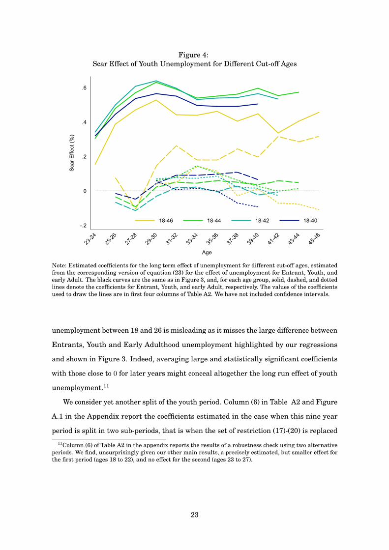
Figure 4:Scar Effect of Youth Unemployment for Different Cut-off Ages

-.2

0

.2

.4

.6

Sca

r Effe

ct (%

)

23-24

25-26

27-28

29-30

31-32

33-34

35-36

37-38

39-40

41-42

43-44

45-46

Age

18-46 18-44 18-42 18-40

Note: Estimated coefficients for the long term effect of unemployment for different cut-off ages, estimatedfrom the corresponding version of equation (23) for the effect of unemployment for Entrant, Youth, andearly Adult. The black curves are the same as in Figure 3, and, for each age group, solid, dashed, and dottedlines denote the coefficients for Entrant, Youth, and early Adult, respectively. The values of the coefficientsused to draw the lines are in first four columns of Table A2. We have not included confidence intervals.

unemployment between 18 and 26 is misleading as it misses the large difference between

Entrants, Youth and Early Adulthood unemployment highlighted by our regressions

and shown in Figure 3. Indeed, averaging large and statistically significant coefficients

with those close to 0 for later years might conceal altogether the long run effect of youth

unemployment.11

We consider yet another split of the youth period. Column (6) in Table A2 and Figure

A.1 in the Appendix report the coefficients estimated in the case when this nine year

period is split in two sub-periods, that is when the set of restriction (17)-(20) is replaced

11Column (6) of Table A2 in the appendix reports the results of a robustness check using two alternativeperiods. We find, unsurprisingly given our other main results, a precisely estimated, but smaller effect forthe first period (ages 18 to 22), and no effect for the second (ages 23 to 27).

23

by

βt1 = βts, s = 18, . . . , 22, t > 24; (26)

βt2 = βts, s = 23, . . . , 26, t > 27; (27)

βts = 0, s > 27, t > s. (28)

Where the subscripts 1 and 2 label the first and the second part of Youth and Early

Adulthood. These are depicted by the aquamarine lines in Figure A.1, also in the

Appendix. These confirm our main finding: early shocks scar, later ones do not.

Columns (5)-(7) of Table 1 confirm that the main message of our paper is robust to

changes in the empirical specification. Column (5) shows that our estimates change

only marginally when, for individuals who report ever being self-employed, we include

observations for years in which they are not self-employed.12 In columns (6) and (7), we

report estimates obtained when missing address information is not inferred as explained

above, by filling missing information with a “fictitious” local area given by their earliest

known address, controlling for the fact that the address is missing. Column (6) simply

replaces all missing addresses with an amorphous “national” address, which captures the

“average national labour market”, with the implicit assumption that everyone had the

same chance to have been at any given location. Column (7) replaces a missing address

with the next recorded address, without accounting for the fact that the information is

in fact missing. In both columns results are very similar to those in column (3), perhaps

with some evidence of a small scar effect in the Youth period (21 to 23) in column (6) only.

This suggests that the results are not sensitive to our treatment of missing addresses.

Figure 4 illustrates the results obtained when we allow the reach of bad shocks ot

extend beyond age 40. The results are once again robust: those observed until 46, for

whom unemployment at age 21-23 has some long term effect. The smaller sample size

(only one cohort is observed until age 46) reduces the precision of the estimates, as

shown in Table A2 in the Appendix.

Oreopoulos et al (2012) study the effect of the business cycle on the importance of the

scarring effect for Canadian graduates. Similar analyses for American and Japanese

12For example, if individual i from cohort entering in 1978 is recorded as self-employed in years 1994 and1997, we drop only these observation from the estimations reported in column (5).

24

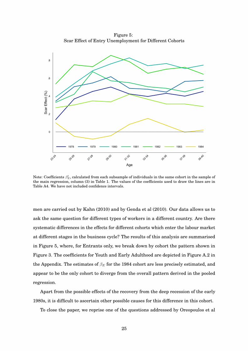
Figure 5:Scar Effect of Entry Unemployment for Different Cohorts

0

.2

.4

.6

.8

Sca

r Effe

ct (%

)

23-24

25-26

27-28

29-30

31-32

33-34

35-36

37-38

39-40

Age

1978 1979 1980 1981 1982 1983 1984

Note: Coefficients βtE , calculated from each subsample of individuals in the same cohort in the sample of

the main regression, column (3) in Table 1. The values of the coefficients used to draw the lines are inTable A4. We have not included confidence intervals.

men are carried out by Kahn (2010) and by Genda et al (2010). Our data allows us to

ask the same question for different types of workers in a different country. Are there

systematic differences in the effects for different cohorts which enter the labour market

at different stages in the business cycle? The results of this analysis are summarised

in Figure 5, where, for Entrants only, we break down by cohort the pattern shown in

Figure 3. The coefficients for Youth and Early Adulthood are depicted in Figure A.2 in

the Appendix. The estimates of βE for the 1984 cohort are less precisely estimated, and

appear to be the only cohort to diverge from the overall pattern derived in the pooled

regression.

Apart from the possible effects of the recovery from the deep recession of the early

1980s, it is difficult to ascertain other possible causes for this difference in this cohort.

To close the paper, we reprise one of the questions addressed by Oreopoulos et al

25

Figure 6:Scar Effect of Entry Unemployment on Individuals of Different Abilities.

0

.2

.4

.6

.8

1

Sca

r Effe

ct (%

)

23-24

25-26

27-28

29-30

31-32

33-34

35-36

37-38

39-40

Age

Top QuintileQuintile 4Quintile 3Quintile 2Bottom Quintile

Note: Coefficients βtE , calculated from the subsamples of individuals made from the quintile according to

the rank determined by their earnings potential. The values of the coefficients used to draw the lines are inTable A4. We have not included confidence intervals.

(2012), namely whether the scarring effect is different for individuals with different

abilities. Following their strategy, we split the sample into five “ability quintiles”, and

allocate individuals to quintiles according to their predicted permanent income estimated

on the basis of the permanent incomes of women who have lived in the same areas at the

same time.13 The results of this exercise for those in the 18-40 age range are presented

in Figure 6, again only for the shocks in the Entry period. Individuals in the lowest

ability group suffer the severest scar. Furthermore, Table A3 in the appendix shows that

the scar effect is not significantly different from 0 for workers in the upper half of the

ability distribution. The worsening of the scar effect for less able workers is a worrying

aspect of our results: youth unemployment seems to reduce most the income of the least

paid workers. This exacerbates the inequality of lifetime incomes.

13Using the income of equivalent women to categorise men into quintiles overlooks the importance ofchild-bearing and part time work as determinants of women’s incomes. It seems however preferable tousing the same data and model both to categorise individuals into quintiles and to estimate the effects foreach quintile.

26

As we discussed in Section 3, we do not observe whether an individual is a university

student. To the extent that students experience low unemployment when aged 18 to 22,

and high earnings later in life, not being able to identify students would bias downward

the scar effect. Given that university that students are probably over-represented in

the higher quartiles of the ability distribution we might be concerned that the lower

scar effect for these quartiles, in part, reflects this bias. However, there are two reasons

to doubt that this is the case. Firstly, we note that only approximately 10% of 18 year

olds went to university in the late 1970s and early 1980s. Secondly, if anything, the scar

effect is larger for more recent cohorts, against a trend of increases in the proportion of

school leavers entering higher education.

6 Concluding remarks

Past unemployment lowers earnings for the rest of a worker’s life. These long term

effects are extensively documented for the US (Table 1 in Couch and Placzeck 2010, p

574, summarises studies using both administrative and survey panel dataset), the UK

(Arulampalam et al 2001 reviews a number of papers of the UK, all of which report

evidence of scarring), and in Japan (Genda et al 2010), among other countries. The

paper by Schmillen and Möller (2012), which follows cohorts of American men born

between 1950 and 1954, also highlights the importance of early shocks for lifetime labour

market outcomes. Our paper contributes to this literature by documenting that not all

unemployment is equal. We report the distinct, permanent effects of being unemployed

at the very beginning of one’s working life.

Knowing that there is a marked difference between the effect of unemployment at

the time of entry and the effect of later unemployment on earnings is different from

knowing why this should be the case. The literature has suggested several possible

causes of a permanent effect of unemployment, ranging from the decay of human capital

(Pissarides 1992), to psychological discouragement or habituation effects (Clark et al

2001), to stigma effects (Vishwanath 1989, Lockwood 1991, Kübler and von Weizsäcker

2003, Biewen and Steffes 2010), to the nature of the search technology (Tatsiramos

2009). Neal (1995) studies the scar effect for workers who subsequently find a new job in

the same sector to identify the extent to which the loss of earnings is due to the sector

27

specific loss of human capital. Given the large differences in long term effects between

Youth and Early Adulthood unemployment we uncover, it would be unsatisfactory if the

only explanation for this difference were that the young are more vulnerable to these

long term effects.

Understanding the causes of these differences would assist the design of policies

specifically directed at relieving youth unemployment. It would also have implications for

macroeconomic policy more generally, given the potentially large difference in the long

term costs and benefits of tackling the unemployment of individuals at different ages. A

promising explanation is the importance of experimentation and learning (Papageorgiou

2014). Wee (2016) argues that those entering the labour market during a recession may

suffer a wage scar. This is because of reduced early career mobility limiting learning

and the accumulation of human capital. This would be in line with our results, which

show that these effects are particularly pronounced for those at the very beginning of

their careers.

28

References

Arulampalam, Wiji, Paul Gregg, and Mary Gregory (2001), “Unemployment scarring.” Economic

Journal, 111, F577–F584.

Bell, D. N. F. and D. G. Blanchflower (2011), “Young people and the Great Recession.” Oxford

Review of Economic Policy, 27, 241–267,

Ben-Porath, Yoram (1967), “The production of human capital and the lifecycle of earnings.”

Journal of Political Economy, 75, 352–365.

Biewen, Martin and Susanne Steffes (2010), “Unemployment persistence: Is there evidence for

stigma effects?” Economics Letters, 106, 188–190.

Blundell, Richard, Antoine Bozio, and Guy Laroque (2013), “Extensive and intensive margins of

labour supply: Work and working hours in the US, the UK and France*.” Fiscal Studies, 34,

1–29,

Cahuc, Pierre, Stéphane Carcillo, Ulf Rinne, and Klaus F Zimmermann (2013), “Youth

unemployment in old Europe: the polar cases of France and Germany.” IZA Journal of

European Labor Studies, 2, 18,

Clark, Andrew, Yannis Georgellis, and Peter Sanfey (2001), “Scarring: The psychological impact

of past unemployment.” Economica, 68, 221–241.

Cornelissen, Thomas (2008), “The stata command felsdvreg to fit a linear model with two

high-dimensional fixed effects.” The Stata Journal, 8, 170–189.

Couch, Kenneth A and Dana W Placzek (2010), “Earnings losses of displaced workers revisited.”

American Economic Review, 100, 572–589.

Cunha, Flavio, James J. Heckman, and Susanne M. Schennach (2010), “Estimating the technology

of cognitive and noncognitive skill formation .” Econometrica, 78, 883–931,

Dickens, Richard and Abigail McKnight (2008a), “Changes in earnings inequality and mobility

in Great Britain 1978/9-2005/6.”

Dickens, Richard and Abigail McKnight (2008b), “Assimilation of migrants into the British

labour market.”

Ellwood, David T (1982), “Teenage unemployment: Permanent scars or temporary blemishes?” In

The Youth Labor Market Problem: Its Nature, Causes, and Consequences (Richard B Freeman

and David A Wise, eds.), 349–390, University of Chicago Press, Chicago.

29

Gardiner, Karen and John Hills (1999), “Policy implications of new data on income mobility .”

The Economic Journal, 109, 91–111,

Genda, Yuji, Ayako Kondo, and Souichi Ohta (2010), “Long-term effects of a recession at labor

market entry in Japan and the United States.” Journal of Human Resources, 45, 157–196,

Goldin, Claudia (2014), “A grand gender convergence: Its last chapter .” American Economic

Review, 104, 1091 – 1119.

Gollin, Douglas (2002), “Getting income shares right.” Journal of Political Economy, 110, 458–

474.

Gosling, Amanda, Paul Johnson, Julian McCrae, and Gillian Paull (1997), “The dynamics of

low pay and unemployment in 1990s Britain.” Technical report, Institute for Fiscal Studies

Working Paper.

Gregg, Paul (2001), “The impact of youth unemployment on adult unemployment in the NCDS.”

Economic Journal, 111, 626–653.

Gregg, Paul and Emma Tominey (2005), “The wage scar from male youth unemployment.” Labour

Economics, 12, 487–509.

Harmon, Colm, Ian Walker, and Niels Westergaard-Nielsen (2001), “Introduction.” In Education

and Earnings in Europe: A Cross-Country Analysis of the Returns to Education (Colm Harmon,

Ian Walker, and Niels Westergaard-Nielsen, eds.), Edward Elgar.

ILO (2012), “Youth Guarantees: A Response to the Youth Employment Crisis?” ILO, Geneva.

Jacobson, Louis S, Robert J LaLonde, and Daniel G Sullivan (1993), “Earnings losses of displaced

workers.” American Economic Review, 83, 685–709.

Jacobson, Louis S, Robert J LaLonde, and Daniel G Sullivan (2005), “Estimating the returns to

community college schooling for displaced workers.” Journal of Econometrics, 125, 271–304.

Kahn, Lisa B. (2010), “The long-term labor market consequences of graduating from college in a

bad economy.” Labour Economics, 17, 303–316,

Kübler, Dorothea and Georg von Weizsäcker (2003), “Information cascades in the labor market.”

Journal of Economics, 80, 211–229.

Lemos, Sara (2013), “Immigrant economic assimilation: Evidence from UK longitudinal data

between 1978 and 2006.” Labour Economics, 24, 339–353,

30

Lemos, Sara (2014), “The immigrant-native earnings gap across the earnings distribution.”

Applied Economics Letters, 22, 361–369,

Lockwood, Ben (1991), “Information externalities in the labour market and the duration of

unemployment.” Review of Economic Studies, 58, 733–753.

Lynch, Lisa M. (1985), “State dependency in youth unemployment.” Journal of Econometrics, 28,

71–84,

Lynch, Lisa M (1989), “The youth labor market in the eighties: Determinants of re-employment

probabilities for young men and women.” Review of Economics and Statistics, 71, 37–45.

Mincer, Jacob (1958), “Investment in human capital and personal income distribution.” Journal

of Political Economy, 66, 281–302.

Mincer, Jacob (1974), Schooling, Experience and Earnings. Columbia University Press, New

York.

Moretti, Enrico (2004), “Estimating the social return to higher education: Evidence from

longitudinal and repeated cross-sectional data.” Journal of Econometrics, 121, 175–212.

Mroz, Thomas A and Timothy H Savage (2006), “The long-term effects of youth unemployment.”

Journal of Human Resources, 41, 259–293.

Neal, Derek (1995), “Industry-specific human capital: Evidence from displaced workers.” Journal

of Labor Economics, 13, 653–677.

Nickell, Stephen, Patricia Jones, and Glenda Quintini (2002), “A picture of job insecurity facing

British men.” The Economic Journal, 112, 1–27,

Oreopoulos, Philip, Till von Wachter, and Andrew Heisz (2012), “The short- and long-term career

effects of graduating in a recession.” American Economic Journal: Applied Economics, 4, 1–29.

Papageorgiou, Theodore (2014), “Learning your comparative advantages.” Review of Economic

Studies, 81, 1263–1295.

Petrongolo, Barbara (2009), “The long-term effects of job search requirements: Evidence from

the UK JSA reform.” Journal of Public Economics, 93, 1234–1253,

Pissarides, Christopher A (1992), “Loss of skill during unemployment and the persistence of

employment shocks.” Quarterly Journal of Economics, 107, 1371–1391.

Ruhm, Christopher J (1991), “Are workers permanently scarred by job displacements?” American

Economic Review, 81, 319–324.

31

Scarpetta, Stefano, Anne Sonnet, and Thomas Manfredi (2010), “Rising Youth Unemployment

During The Crisis ” OECD Social, Employment and Migration Working Papers, 106, OECD

Publishing.

Schmillen, Achim and Joachim Möller (2012), “Distribution and determinants of lifetime

unemployment.” Labour Economics, 19, 33–47.

Stevens, Ann Huff (1997), “Persistent effects of job displacement: The importance of multiple job

losses.” Journal of Labor Economics, 15, 165–188.

Tatsiramos, Konstantinos (2009), “Unemployment insurance in Europe: Unemployment duration

and subsequent employment stability.” Journal of the European Economic Association, 7,

1225–1260.

Vishwanath, Tara (1989), “Job search, stigma effect, and escape rate from unemployment.”

Journal of Labor Economics, 7, 487–502.

Wee, Shu Lin (2010), “Delayed learning and human capital accumulation: The cost of entering

the job market during a recession ” mimeo.

32

Appendix: Additional Tables and Figures

Figure A.1:The scar effect of youth unemployment

-.2

0

.2

.4

.6

Sca

r Effe

ct (%

)

23-24

25-26

27-28

29-30

31-32

33-34

35-36

37-38

39-40

Age

Entrant: 18-20 Youth: 21-23 Early Adult: 24-26Aggregate: 18-26 2-Way Split: 18-22 2-Way Split: 23-27

Note: The blue lines report the estimated coefficients from equation (23) for the effect of Entrant, Youth,and early Adulthood unemployment, βt

E (solid line), βtY (dashed line), and βt

A (dotted line). The light grenline depicts the coefficients when (23) is estimated with the restrictions (24)-(25). These are the same linesas in Figure 3, without the confidence intervals. The aquamarine lines are the coefficients when (23) isestimated with the restrictions (26)-(28). For all lines, the dashed lines include the 10% confidence intervals.

A1

Table A1:Summary Statistics for individuals in Sample for Table A1.

1960 1961 1962 1963 1964 1965 1966 Total

u Age 18-20 9.66 13.25 18.59 22.11 25.50 25.78 23.10 19.58

sd 19.76 23.73 28.91 31.74 32.78 32.07 29.81 29.24

21-23 16.60 19.02 20.36 20.40 20.70 18.93 16.02 18.88

sd 29.17 30.90 31.72 31.46 30.63 29.89 27.81 30.32

24-26 15.08 15.00 14.25 13.77 14.29 15.85 16.31 14.92

sd 29.48 28.68 27.78 27.31 28.46 29.51 30.03 28.75

Earn 23-24 12229 11998 11936 11932 12454 13114 13313 12409

sd 6875 7235 7929 7649 8163 8693 8221 7848

25-26 13800 13890 14417 14778 14791 14544 14023 14316

sd 8476 8687 9728 9040 9722 10614 9544 9418

27-28 16233 16881 16850 16095 15494 15405 15546 16093

sd 10624 10783 11446 11370 11400 12040 11883 11376

29-30 18306 18208 17337 16631 16737 16869 16508 17242

sd 11763 14924 12915 12274 13979 13191 14337 13396

31-32 18378 18416 18269 17524 17521 17729 18042 17991

sd 12441 12905 13557 14306 15170 15640 16952 14463

33-34 19205 19441 18795 17972 18529 19914 20876 19236

sd 13710 15307 14416 15829 15476 18793 21797 16644

35-36 19451 19821 19695 19591 20709 22203 22675 20559

sd 14389 17442 16460 18019 18760 23908 23121 19094

37-38 20461 21659 21830 21857 22041 23414 22401 21936

sd 16010 24366 20003 27207 20625 24809 20905 22273

39-40 22704 23462 23058 22236 22202 24444 23302 23053

sd 22904 25356 20691 26052 23458 32200 26050 25398

41-42 23638 23877 23394 22036 22075 0 0 23019

sd 20546 27446 23736 22485 22663 0 0 23533

43-44 23794 23936 23818 0 0 0 0 23850

sd 21963 22492 26957 0 0 0 0 23935

45-46 24348 0 0 0 0 0 0 24348

sd 28231 0 0 0 0 0 0 28231

Benef 23-24 0.29 0.31 0.33 0.33 0.33 0.30 0.29 0.31

25-26 0.26 0.27 0.26 0.25 0.28 0.31 0.31 0.28

27-28 0.22 0.21 0.23 0.26 0.29 0.31 0.30 0.26

29-30 0.20 0.23 0.27 0.28 0.30 0.30 0.30 0.26

31-32 0.24 0.25 0.27 0.30 0.29 0.28 0.26 0.27

33-34 0.26 0.26 0.28 0.28 0.28 0.26 0.26 0.27

35-36 0.26 0.25 0.25 0.28 0.28 0.28 0.27 0.27

37-38 0.24 0.24 0.25 0.29 0.29 0.27 0.25 0.26

39-40 0.25 0.25 0.26 0.28 0.27 0.24 0.23 0.26

41-42 0.26 0.25 0.24 0.25 0.25 0 0 0.25

43-44 0.24 0.22 0.24 0 0 0 0 0.23

45-46 0.22 0 0 0 0 0 0 0.22

N 2065 2154 2164 2089 1985 1966 2001 14424

Note: The upper part reports the unemployment rate of UK male individuals born in 1960-1966 at age18-20, 21-23 and 24-26. the middle part their average yearly earnings at ages 23-24 to 45-46. The thirdpart is the proportion who claimed some of the benefits available

A2

Figure A.2:Scar Effects of Youth and Early Adult Unemployment for Different Cohorts

-.4

-.2

0

.2

.4

Sca

r Effe

ct (%

)

25-26

27-28

29-30

31-32

33-34

35-36

37-38

39-40

Age

-.4

-.2

0

.2

.4

Sca

r Effe

ct (%

)

25-26

27-28

29-30

31-32

33-34

35-36

37-38

39-40

Age

1978 1979 1980 1981 1982 1983 1984

Note: The lines report the estimated coefficients from (23) for the effect of Youth, and Early Adulthoodunemployment corresponding to those in Figure 5. That is the coefficients βt

Y and βtA, calculated from each

subsample of individuals in the same cohort in the sample of the main regression, column 3 in Table 1.

A3

Figure A.3:Scar Effects of Youth and Early Adult Unemployment on

Individuals of Different Abilities.

-.3

-.2

-.1

0

.1

.2

Sca

r Effe

ct (%

)

25-26

27-28

29-30

31-32

33-34

35-36

37-38

39-40

Age

-.3

-.2

-.1

0

.1

.2

Sca

r Effe

ct (%

)

29-30

31-32

33-34

35-36

37-38

39-40

Age

Top Quintile Quintile 4 Quintile 3 Quintile 2 Bottom Quintile

Note: The lines report the estimated coefficients from (23) for the effect of Youth, and Early Adulthoodunemployment corresponding to those in Figure 6. That is the coefficients βt

Y and βtA, calculated for each

subsample of individuals in the same ability quintile according to the rank determined by the earningspotentials of women who have lived in the same places at the same time.

A4

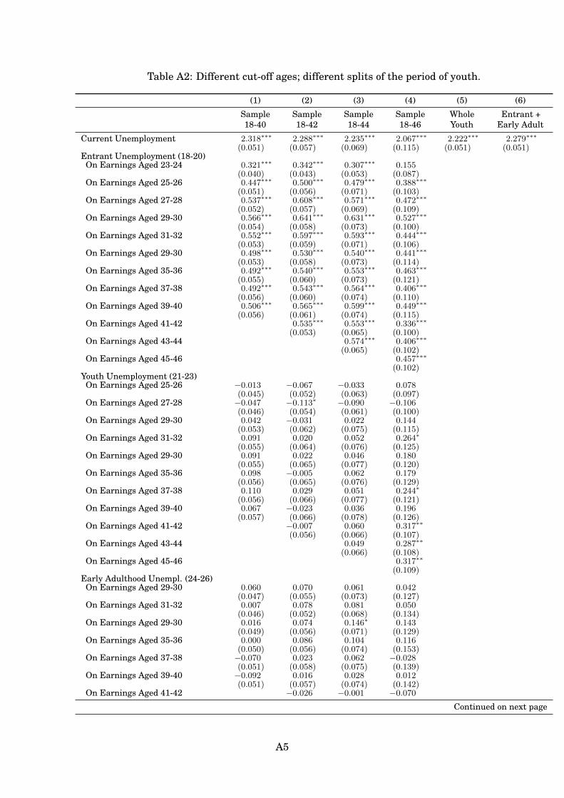
Table A2: Different cut-off ages; different splits of the period of youth.

(1) (2) (3) (4) (5) (6)

Sample18-40

Sample18-42

Sample18-44

Sample18-46

WholeYouth

Entrant +Early Adult

Current Unemployment 2.318∗∗∗ 2.288∗∗∗ 2.235∗∗∗ 2.067∗∗∗ 2.222∗∗∗ 2.279∗∗∗

(0.051) (0.057) (0.069) (0.115) (0.051) (0.051)Entrant Unemployment (18-20)On Earnings Aged 23-24 0.321∗∗∗ 0.342∗∗∗ 0.307∗∗∗ 0.155

(0.040) (0.043) (0.053) (0.087)On Earnings Aged 25-26 0.447∗∗∗ 0.500∗∗∗ 0.479∗∗∗ 0.388∗∗∗

(0.051) (0.056) (0.071) (0.103)On Earnings Aged 27-28 0.537∗∗∗ 0.608∗∗∗ 0.571∗∗∗ 0.472∗∗∗

(0.052) (0.057) (0.069) (0.109)On Earnings Aged 29-30 0.566∗∗∗ 0.641∗∗∗ 0.631∗∗∗ 0.527∗∗∗

(0.054) (0.058) (0.073) (0.100)On Earnings Aged 31-32 0.552∗∗∗ 0.597∗∗∗ 0.593∗∗∗ 0.444∗∗∗

(0.053) (0.059) (0.071) (0.106)On Earnings Aged 29-30 0.498∗∗∗ 0.530∗∗∗ 0.540∗∗∗ 0.441∗∗∗

(0.053) (0.058) (0.073) (0.114)On Earnings Aged 35-36 0.492∗∗∗ 0.540∗∗∗ 0.553∗∗∗ 0.463∗∗∗

(0.055) (0.060) (0.073) (0.121)On Earnings Aged 37-38 0.492∗∗∗ 0.543∗∗∗ 0.564∗∗∗ 0.406∗∗∗

(0.056) (0.060) (0.074) (0.110)On Earnings Aged 39-40 0.506∗∗∗ 0.565∗∗∗ 0.599∗∗∗ 0.449∗∗∗

(0.056) (0.061) (0.074) (0.115)On Earnings Aged 41-42 0.535∗∗∗ 0.553∗∗∗ 0.336∗∗∗

(0.053) (0.065) (0.100)On Earnings Aged 43-44 0.574∗∗∗ 0.406∗∗∗

(0.065) (0.102)On Earnings Aged 45-46 0.457∗∗∗

(0.102)Youth Unemployment (21-23)On Earnings Aged 25-26 −0.013 −0.067 −0.033 0.078

(0.045) (0.052) (0.063) (0.097)On Earnings Aged 27-28 −0.047 −0.113∗ −0.090 −0.106

(0.046) (0.054) (0.061) (0.100)On Earnings Aged 29-30 0.042 −0.031 0.022 0.144

(0.053) (0.062) (0.075) (0.115)On Earnings Aged 31-32 0.091 0.020 0.052 0.264∗

(0.055) (0.064) (0.076) (0.125)On Earnings Aged 29-30 0.091 0.022 0.046 0.180

(0.055) (0.065) (0.077) (0.120)On Earnings Aged 35-36 0.098 −0.005 0.062 0.179

(0.056) (0.065) (0.076) (0.129)On Earnings Aged 37-38 0.110 0.029 0.051 0.244∗

(0.056) (0.066) (0.077) (0.121)On Earnings Aged 39-40 0.067 −0.023 0.036 0.196

(0.057) (0.066) (0.078) (0.126)On Earnings Aged 41-42 −0.007 0.060 0.317∗∗

(0.056) (0.066) (0.107)On Earnings Aged 43-44 0.049 0.287∗∗

(0.066) (0.108)On Earnings Aged 45-46 0.317∗∗

(0.109)Early Adulthood Unempl. (24-26)On Earnings Aged 29-30 0.060 0.070 0.061 0.042

(0.047) (0.055) (0.073) (0.127)On Earnings Aged 31-32 0.007 0.078 0.081 0.050

(0.046) (0.052) (0.068) (0.134)On Earnings Aged 29-30 0.016 0.074 0.146∗ 0.143

(0.049) (0.056) (0.071) (0.129)On Earnings Aged 35-36 0.000 0.086 0.104 0.116

(0.050) (0.056) (0.074) (0.153)On Earnings Aged 37-38 −0.070 0.023 0.062 −0.028

(0.051) (0.058) (0.075) (0.139)On Earnings Aged 39-40 −0.092 0.016 0.028 0.012

(0.051) (0.057) (0.074) (0.142)On Earnings Aged 41-42 −0.026 −0.001 −0.070

Continued on next page

A5

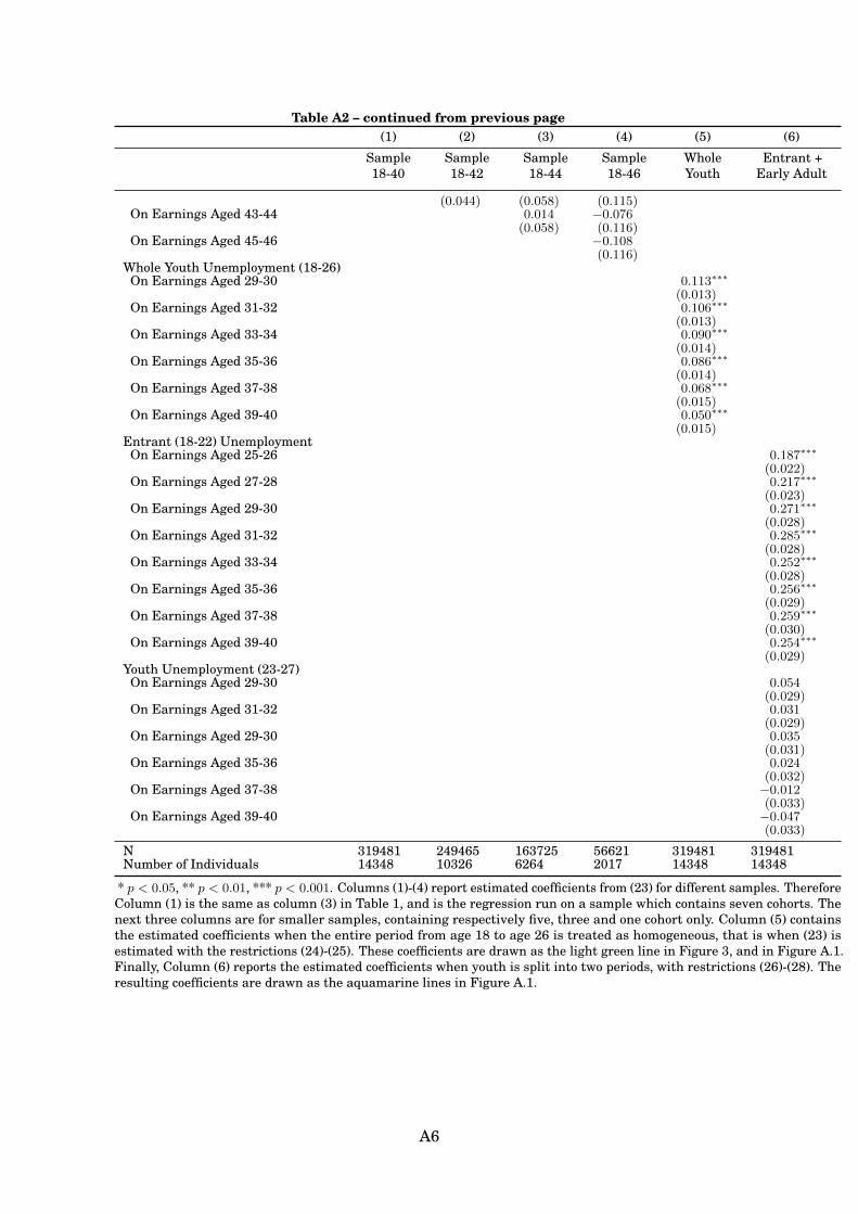
Table A2 – continued from previous page(1) (2) (3) (4) (5) (6)

Sample18-40

Sample18-42

Sample18-44

Sample18-46

WholeYouth

Entrant +Early Adult

(0.044) (0.058) (0.115)On Earnings Aged 43-44 0.014 −0.076

(0.058) (0.116)On Earnings Aged 45-46 −0.108

(0.116)Whole Youth Unemployment (18-26)On Earnings Aged 29-30 0.113∗∗∗

(0.013)On Earnings Aged 31-32 0.106∗∗∗

(0.013)On Earnings Aged 33-34 0.090∗∗∗

(0.014)On Earnings Aged 35-36 0.086∗∗∗

(0.014)On Earnings Aged 37-38 0.068∗∗∗

(0.015)On Earnings Aged 39-40 0.050∗∗∗

(0.015)Entrant (18-22) UnemploymentOn Earnings Aged 25-26 0.187∗∗∗

(0.022)On Earnings Aged 27-28 0.217∗∗∗

(0.023)On Earnings Aged 29-30 0.271∗∗∗

(0.028)On Earnings Aged 31-32 0.285∗∗∗

(0.028)On Earnings Aged 33-34 0.252∗∗∗

(0.028)On Earnings Aged 35-36 0.256∗∗∗

(0.029)On Earnings Aged 37-38 0.259∗∗∗

(0.030)On Earnings Aged 39-40 0.254∗∗∗

(0.029)Youth Unemployment (23-27)On Earnings Aged 29-30 0.054

(0.029)On Earnings Aged 31-32 0.031

(0.029)On Earnings Aged 29-30 0.035

(0.031)On Earnings Aged 35-36 0.024

(0.032)On Earnings Aged 37-38 −0.012

(0.033)On Earnings Aged 39-40 −0.047

(0.033)

N 319481 249465 163725 56621 319481 319481Number of Individuals 14348 10326 6264 2017 14348 14348

* p < 0.05, ** p < 0.01, *** p < 0.001. Columns (1)-(4) report estimated coefficients from (23) for different samples. ThereforeColumn (1) is the same as column (3) in Table 1, and is the regression run on a sample which contains seven cohorts. Thenext three columns are for smaller samples, containing respectively five, three and one cohort only. Column (5) containsthe estimated coefficients when the entire period from age 18 to age 26 is treated as homogeneous, that is when (23) isestimated with the restrictions (24)-(25). These coefficients are drawn as the light green line in Figure 3, and in Figure A.1.Finally, Column (6) reports the estimated coefficients when youth is split into two periods, with restrictions (26)-(28). Theresulting coefficients are drawn as the aquamarine lines in Figure A.1.

A6

Table A3:Results For Different Ability Quintiles

(1) (2) (3) (4) (5)Bottom Quartile 2nd Quartile 3rd Quartile 4th Quartile Top Quartile

Current Unemployment 4.453∗∗∗ 1.822∗∗∗ 0.887∗∗∗ 0.742∗∗∗ 0.381∗∗

(0.205) (0.153) (0.136) (0.137) (0.124)Entrant Unemployment (18-20)On Earnings Aged 23-24 0.487∗ 0.276 0.056 0.158 0.166

(0.225) (0.186) (0.167) (0.145) (0.145)On Earnings Aged 25-26 0.541 0.425∗ 0.237 0.211 0.351∗

(0.289) (0.208) (0.215) (0.181) (0.177)On Earnings Aged 27-28 0.795∗∗ 0.371 0.351 0.261 0.287

(0.289) (0.220) (0.235) (0.163) (0.173)On Earnings Aged 29-30 1.061∗∗∗ 0.423 0.266 0.205 0.271

(0.318) (0.216) (0.204) (0.169) (0.173)On Earnings Aged 31-32 0.741∗ 0.353 0.227 0.263 0.216

(0.331) (0.234) (0.206) (0.161) (0.168)On Earnings Aged 29-30 0.694∗ 0.344 0.222 0.259 0.233

(0.337) (0.222) (0.200) (0.158) (0.168)On Earnings Aged 35-36 0.722∗ 0.421 0.202 0.228 0.219

(0.338) (0.224) (0.197) (0.155) (0.169)On Earnings Aged 37-38 0.616 0.475∗ 0.203 0.254 0.220

(0.356) (0.219) (0.197) (0.155) (0.165)On Earnings Aged 39-40 0.610 0.382 0.266 0.249 0.205

(0.357) (0.231) (0.202) (0.157) (0.164)Youth Unemployment (21-23)On Earnings Aged 25-26 0.223 −0.186 −0.129 −0.076 −0.102

(0.230) (0.173) (0.188) (0.172) (0.142)On Earnings Aged 27-28 −0.056 −0.061 −0.248 −0.172 −0.142

(0.249) (0.182) (0.198) (0.152) (0.144)On Earnings Aged 29-30 −0.089 0.024 −0.184 −0.060 −0.039

(0.340) (0.194) (0.184) (0.174) (0.144)On Earnings Aged 31-32 0.027 0.216 −0.117 −0.102 0.023

(0.347) (0.204) (0.166) (0.166) (0.139)On Earnings Aged 29-30 0.023 0.045 −0.158 −0.088 0.014

(0.359) (0.189) (0.167) (0.160) (0.137)On Earnings Aged 35-36 −0.091 0.054 −0.165 −0.091 0.019

(0.384) (0.189) (0.167) (0.164) (0.140)On Earnings Aged 37-38 0.181 −0.029 −0.141 −0.096 −0.009

(0.402) (0.191) (0.169) (0.167) (0.139)On Earnings Aged 39-40 −0.011 −0.022 −0.159 −0.102 0.008

(0.381) (0.211) (0.173) (0.164) (0.144)Early Adulthood Unemployment(24-26)

On Earnings Aged 29-30 0.184 −0.071 0.030 0.028 −0.204(0.264) (0.160) (0.133) (0.132) (0.138)

On Earnings Aged 31-32 0.054 −0.194 −0.127 −0.056 −0.239(0.262) (0.159) (0.121) (0.134) (0.139)

On Earnings Aged 29-30 −0.021 −0.187 −0.056 −0.113 −0.314∗

(0.289) (0.146) (0.118) (0.133) (0.136)On Earnings Aged 35-36 0.088 −0.194 −0.036 −0.104 −0.320∗

(0.303) (0.145) (0.117) (0.136) (0.136)On Earnings Aged 37-38 −0.212 −0.117 −0.027 −0.083 −0.296∗

(0.316) (0.149) (0.125) (0.138) (0.136)On Earnings Aged 39-40 −0.308 −0.145 −0.055 −0.047 −0.246

(0.326) (0.163) (0.121) (0.128) (0.132)

Observations 58,036 57,959 57,974 57,926 57,882Number of Individuals 2,583 2,540 2,529 2,522 2,519

* p < 0.05, ** p < 0.01, *** p < 0.001. Coefficients for the estimation of (23), the same as the main regression, column (3)in Table 1, estimated from each subsample of individuals in the same ability quintile according to the rank determinedby their earnings potential. The coefficients in the top block are plotted in Figure 6, those in the other two blocks inFigure A.3.

A7

Table A4:Results For Individual Cohorts

(1) (2) (3) (4) (5) (6) (7)1978 1979 1980 1981 1982 1983 1984

Current Unemployment 2.050∗∗∗ 2.124∗∗∗ 2.388∗∗∗ 2.381∗∗∗ 2.439∗∗∗ 2.489∗∗∗ 2.557∗∗∗

(0.131) (0.118) (0.142) (0.141) (0.139) (0.149) (0.125)Entrant Unemployment (18-20)On Earnings Aged 23-24 0.137 0.343∗∗∗ 0.389∗∗∗ 0.331∗∗∗ 0.536∗∗∗ 0.272 0.102

(0.085) (0.085) (0.102) (0.095) (0.114) (0.143) (0.182)On Earnings Aged 25-26 0.367∗∗∗ 0.506∗∗∗ 0.541∗∗∗ 0.421∗∗∗ 0.752∗∗∗ 0.302 −0.048

(0.100) (0.127) (0.141) (0.119) (0.132) (0.170) (0.204)On Earnings Aged 27-28 0.451∗∗∗ 0.546∗∗∗ 0.684∗∗∗ 0.675∗∗∗ 0.731∗∗∗ 0.348∗ −0.080

(0.112) (0.116) (0.138) (0.136) (0.146) (0.167) (0.212)On Earnings Aged 29-30 0.502∗∗∗ 0.617∗∗∗ 0.763∗∗∗ 0.570∗∗∗ 0.857∗∗∗ 0.338 −0.043

(0.103) (0.118) (0.154) (0.137) (0.140) (0.181) (0.210)On Earnings Aged 31-32 0.424∗∗∗ 0.489∗∗∗ 0.830∗∗∗ 0.552∗∗∗ 0.787∗∗∗ 0.421∗ 0.084

(0.113) (0.114) (0.148) (0.144) (0.139) (0.169) (0.210)On Earnings Aged 29-30 0.397∗∗ 0.477∗∗∗ 0.739∗∗∗ 0.506∗∗∗ 0.655∗∗∗ 0.367∗ 0.151

(0.124) (0.120) (0.144) (0.137) (0.135) (0.166) (0.216)On Earnings Aged 35-36 0.431∗∗∗ 0.446∗∗∗ 0.763∗∗∗ 0.488∗∗∗ 0.703∗∗∗ 0.314 0.075

(0.130) (0.125) (0.136) (0.145) (0.139) (0.177) (0.215)On Earnings Aged 37-38 0.399∗∗∗ 0.564∗∗∗ 0.708∗∗∗ 0.450∗∗ 0.722∗∗∗ 0.313 −0.004

(0.120) (0.129) (0.151) (0.151) (0.141) (0.173) (0.223)On Earnings Aged 39-40 0.452∗∗∗ 0.574∗∗∗ 0.749∗∗∗ 0.503∗∗∗ 0.646∗∗∗ 0.284 0.020

(0.125) (0.130) (0.152) (0.152) (0.145) (0.182) (0.223)Youth Unemployment (21-23)On Earnings Aged 25-26 0.089 −0.036 −0.239 −0.244∗ −0.120 0.118 0.307∗∗

(0.095) (0.104) (0.130) (0.122) (0.152) (0.127) (0.119)On Earnings Aged 27-28 −0.096 −0.020 −0.183 −0.266 −0.129 0.106 0.276∗

(0.099) (0.098) (0.126) (0.155) (0.163) (0.127) (0.120)On Earnings Aged 29-30 0.164 0.128 −0.329∗ −0.318 −0.111 0.247 0.345∗∗

(0.112) (0.123) (0.163) (0.180) (0.167) (0.158) (0.116)On Earnings Aged 31-32 0.307∗ 0.114 −0.379∗ −0.177 −0.079 0.251 0.331∗

(0.133) (0.121) (0.162) (0.183) (0.189) (0.152) (0.129)On Earnings Aged 29-30 0.251 0.146 −0.380∗ −0.265 −0.004 0.234 0.347∗∗

(0.129) (0.129) (0.159) (0.184) (0.176) (0.155) (0.123)On Earnings Aged 35-36 0.227 0.162 −0.304 −0.261 −0.239 0.320∗ 0.420∗∗

(0.137) (0.123) (0.159) (0.180) (0.178) (0.149) (0.131)On Earnings Aged 37-38 0.264∗ 0.083 −0.274 −0.093 −0.147 0.246 0.363∗∗

(0.131) (0.130) (0.170) (0.192) (0.176) (0.154) (0.126)On Earnings Aged 39-40 0.183 0.056 −0.291 −0.279 −0.199 0.311∗ 0.305∗

(0.133) (0.129) (0.180) (0.189) (0.182) (0.155) (0.134)Early Adulthood Unemployment(24-26)

On Earnings Aged 29-30 0.021 −0.053 0.247∗ 0.179 −0.042 −0.029 0.057(0.127) (0.135) (0.121) (0.103) (0.126) (0.143) (0.120)

On Earnings Aged 31-32 0.035 0.007 0.243∗ 0.123 −0.069 −0.211 −0.136(0.146) (0.115) (0.112) (0.097) (0.137) (0.143) (0.125)

On Earnings Aged 29-30 0.120 0.047 0.320∗∗ −0.000 −0.142 −0.190 −0.056(0.139) (0.132) (0.117) (0.116) (0.150) (0.144) (0.132)

On Earnings Aged 35-36 0.111 0.035 0.198 0.107 −0.083 −0.261 −0.118(0.165) (0.127) (0.119) (0.111) (0.137) (0.143) (0.139)

On Earnings Aged 37-38 −0.024 0.027 0.198 −0.054 −0.092 −0.401∗∗ −0.195(0.151) (0.138) (0.133) (0.117) (0.142) (0.136) (0.138)

On Earnings Aged 39-40 0.033 −0.071 0.152 0.041 −0.086 −0.450∗∗ −0.291∗

(0.154) (0.137) (0.128) (0.113) (0.153) (0.138) (0.143)

N 46222 48013 48222 46073 43583 43203 44165Number of Individuals 2057 2143 2152 2076 1972 1954 1994

* p < 0.05, ** p < 0.01, *** p < 0.001. Coefficients for the estimation of (23), the same as the main regression,column (3) in Table 1, estimated from each subsample of individuals according to the year of entry in the labourmarket. The coefficients in the top block are plotted in Figure 5, those in the other two blocks in Figure A.2.

A8

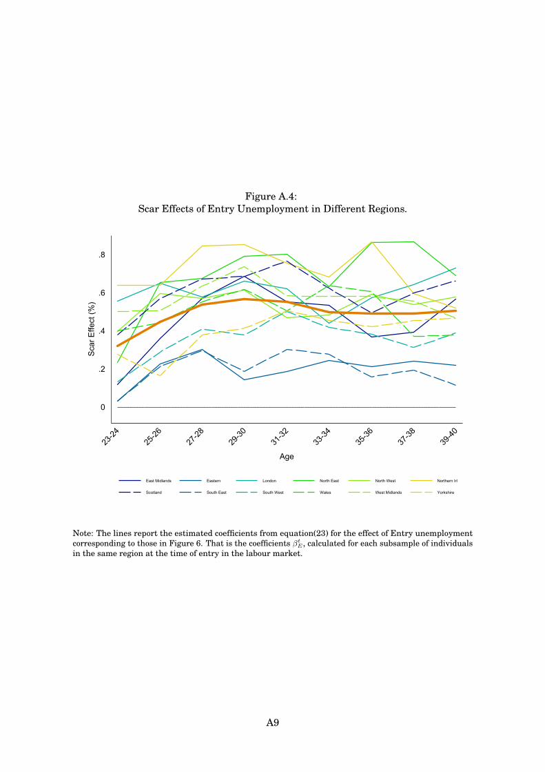
Figure A.4:Scar Effects of Entry Unemployment in Different Regions.

0

.2

.4

.6

.8

Sca

r Effe

ct (%

)

23-24

25-26

27-28

29-30

31-32

33-34

35-36

37-38

39-40

Age

East Midlands Eastern London North East North West Northern Irl

Scotland South East South West Wales West Midlands Yorkshire

Note: The lines report the estimated coefficients from equation(23) for the effect of Entry unemploymentcorresponding to those in Figure 6. That is the coefficients βt

E , calculated for each subsample of individualsin the same region at the time of entry in the labour market.

A9

Figure A.5:Scar Effects of Youth and Early Adult Unemployment in Different Regions.

-.4

-.2

0

.2

.4

Sca

r Effe

ct (%

)

25-26

27-28

29-30

31-32

33-34

35-36

37-38

39-40

Age

-.6

-.4

-.2

0

.2

.4

Sca

r Effe

ct (%

)

29-30

31-32

33-34

35-36

37-38

39-40

Age

East Midlands Eastern London North East North West Northern Irl

Scotland South East South West Wales West Midlands Yorkshire

Note: The lines report the estimated coefficients from equation(23) for the effect of Youth, and EarlyAdulthood unemployment corresponding to those in Figure 6. That is the coefficients βt

Y and βtA, calculated

from each subsample of individuals in the same region at the time of entry in the labour market.

A10