Embed Size (px)
Citation preview

CARD Technical Reports CARD Reports and Working Papers
3-1991
The World Feed-Grains Trade Model:Specification, Estimation, and ValidationMichael D. HelmarIowa State University
S. DevadossIowa State University
William H. MeyersIowa State University
Follow this and additional works at: http://lib.dr.iastate.edu/card_technicalreports
Part of the Agricultural and Resource Economics Commons, Agricultural Economics Commons,and the Econometrics Commons
This Article is brought to you for free and open access by the CARD Reports and Working Papers at Iowa State University Digital Repository. It hasbeen accepted for inclusion in CARD Technical Reports by an authorized administrator of Iowa State University Digital Repository. For moreinformation, please contact [email protected].
Recommended CitationHelmar, Michael D.; Devadoss, S.; and Meyers, William H., "The World Feed-Grains Trade Model: Specification, Estimation, andValidation" (1991). CARD Technical Reports. 28.http://lib.dr.iastate.edu/card_technicalreports/28

The World Feed-Grains Trade Model: Specification, Estimation, andValidation
AbstractThe feed-grains trade model is one of the three models in the world trade modeling system developed,updated, and maintained by the Center for Agricultural and Rural Development (CARD). The other twocommodity trade models are for wheat and the soybeans complex. The three world models are relatedthrough cross-price linkages in the supply and demand components of these models, yet each model can besolved independently. In general, however, all three trade models are solved iteratively to obtain asimultaneous solution. Equilibrium prices, quantities of supply and demand, and net trade are determined byequating excess demands and supplies across regions and explicitly linking prices in each region to a worldreference price.
DisciplinesAgricultural and Resource Economics | Agricultural Economics | Econometrics
This article is available at Iowa State University Digital Repository: http://lib.dr.iastate.edu/card_technicalreports/28

The World Feed-Grains Trade Model: Specification, Estimation, and Validation
by Michael Helmar, S. Devadoss, and William H. Meyers
Technical Report 91-TR 78 March 1991
Center for Agricultural and Rural Development Iowa State University
Ames, Iowa 50011
Michael He/mar is a research associate; 5. Devadoss is an adjunct assistant professor; and William H. Meyers is a professor of economics and associate director of CARD.
Support for this research was provided in part by the Food and Agricultural Policy Research Institute (FAPRI). FAPRI is a joint policy-analysis program at Iowa State University and the University of Missouri-Columbia.

Figures
Tables
Introduction
Modeling Approach
Specification • . Theoretical Foundations Demand Data Sources
Empirical Results United States Submodel Canadian Submodel Australian Submodel Argentine Submodel . The European Community Submodel Thai Submodel . . • . South African Submodel Soviet Submodel Chinese Submodel . • . Eastern European Submodel Japanese Submodel Brazilian Submodel Mexican Submodel . Egyptian Submodel Indian Submodel Nigerian Submodel Saudi Arabian Submodel High-Income East Asian Submodel "Other Asia" Submodel •••.
iii
CONTENTS
"Other Africa and Middle East" Submodel "Other Latin America" Submodel Rest-of-the-World Submodel
Evaluation
Uses of the Model
Appendix: Simulation Statistics from the Dynamic Simulation of the World Feed-Grains Trade Model
References
v
v
l
2
7 7
12 15
16 17 42 49 56 62 70 74 79 80 80 87 98 98
108 112 112 117 117 122 122 122 128
133
135
145
151

1.
2.
1.
2.
3 0
4.
5.
6.
7.
8.
9.
10.
11.
12.
13.
14.
15 0
16.
17 0
v
FIGURES
Representation of the structure of the world feed-grains trade model . . . . • . . • . . . . . . • . • . • Determination of equilibrium prices and quantities in the CARD/FAPRI agricultural trade models ......•....
TABLES
Structural parameter estimates of the u.s. feed-grains submodel 0 0 0 0 0 0 0
Structural parameter estimates of the Canadian feed-grains submodel 0 0 0 0 0 0
Structural parameter estimates of the Australian feed-grains submodel 0 0 0 0 0 0
Structural parameter estimates of the Argentine feed-grains submodel 0 0 0 0 0
Structural parameter estimates of the European Community feed-grains submodel 0 0 0
Structural parameter estimates of the Thai feed-grains submodel 0 0 0 0 0
Structural parameter estimates of the South African feed-grains submodel 0
Structural parameter estimates of the Soviet feed-grains submodel 0 0 0 0 0 0 0 0
Structural parameter estimates of the Chinese feed-grains submodel 0 0 0 0 0 0 0
Structural parameter estimates of the Eastern European feed-grains submodel 0 0 0 0
Structural parameter estimates of the Japanese feed-grains submodel 0 0 0 0 0
Structural parameter estimates of the Brazilian feed-grains submodel 0 0 0 0 0 0 0 0 0 0 0
Structural parameter estimates of the Mexican feed-grains submodel 0 0 0 0 0 0
Structural parameter estimates of the Egyptian feed-grains submodel 0 0 0 0
Structural parameter estimates of the Indian feed-grains submodel 0 0 0 0 0
Structural parameter estimates of the Nigerian feed-grains submodel Structural parameter estimates of the Saudi Arabian feed-grains submodel
3
5
18
43
50
57
65
71
75
81
83
85
88
99
102
109
113
115
118

vi
18. Structural parameter estimates of the high-income East Asian feed-grains submodel . . • . . . . . .
19. Structural parameter estimates of the "Other Asia" feed-grains submodel • • . . • • . . • . . .
20. Structural parameter estimates of the "Other Asia and Middle East" feed-grains submodel . . . . .
21. Structural parameter estimates of the "Other Latin America" feed-grains submodel ....•..
22. Structural parameter estimates of the ROW feed-grains submodel . • . . . . . . . . . . . . . . . . . . • . .
23. Summary of estimated production elasticities from the feed-grains trade model . . . • • . . . . . . . . . .
24. Summary of estimated domestic demand elasticities from the feed-grains trade model ·• •..•......
25. Key price-transmission elasticities of feed-grains prices with respect to U.S. feed-grains prices ..•.•••..
120
123
124
126
129
136
138
140

Introduction
The feed-grains trade model is one of the three models in the world trade
modeling system developed, updated, and maintained by the Center for
Agricultural and Rural Development (CARD). The other two commodity trade models
are for wheat and the soybeans complex. The three world models are related
through cross-price linkages in the supply and demand components of these
models, yet each model can be solved independently. In general, however, all
three trade models are solved iteratively to obtain a simultaneous solution.
Equilibrium prices, quantities of supply and demand, and net trade are
determined by equating excess denands and supplies across regions and explicitly
linking prices in each region to a world reference price.
The trade models, along with the U.S. domestic crops and livestock models
maintained by CARD, have been used extensively to examine the impact of domestic
and foreign farm-policy changes and of exogenous shocks. Policy scenarios
evaluated with this modeling system have ranged from very restrictive mandatory
supply control to complete elimination of domestic and foreign farm programs.
The models are also used periodically to project key agricultural variables over
10-year periods. The analyses of impacts of exogenous shocks include technology
shocks, such as yield changes; changes in macroeconomic variables, such as
income growth, inflation rate, or exchange rates; and external policy
shocks, such as tariffs and subsidies. Requests for policy research have come
from the U.S. Congress, the National Governors' Association, the U.S. Department
of Agriculture, the U.S. Agency for International Development, Agriculture
Canada, the Commission of the European Communities, and farm organizations
2
including the National Corn Growers Association, the Iowa Corn Promotion Board,
the Iowa Soybean Promotion Board, and the National Pork Producers' Council.
The organization of this documentation is as follows. In the next section,
model structure is presented, along with national and regional details. The
third section contains theoretical foundations for model specification. The
fourth section presents estimation procedures and results. In the fifth
section, elasticity estimates are reported, and the model is validated using
simulation results. A brief discussion of the applications and limitations of
the model is presented in the final section.
Modeling Approach
The purposes of this section are to describe the structure of the
feed-grains model and to explain national and regional disaggregation.
The overall structure of the model is based upon the dissertation research
of Bahrenian (1987). The model is a nonspatial partial equilibrium
model--nonspatial because it does not identify trade flows between specific
regions, and in partial equilibrium because only one commodity is modeled.
Figure l illustrates the structural components of the model, which includes
domestic supply and demand functions for major trading and producing countries
and regions. Equilibrium prices, quantities, and net trade are determined by
equating excess demands and supplies across regions and explicitly linking
prices in each region to a world price. Except where they are set by
governments, domestic prices are linked to world prices via price-linkage
equations including those concerning bilateral exchange rates and
transfer-service margins. Where some degree of insulation of domestic prices
from external market conditions exists, trade flows are restricted. The

Generally Exogenous
Otherwise:
r--------------------------------~--------------, 1 I 1 1 I I 1 I 1 1 I 1 1 I I
_L I I l' I I
t I
Gov't Policy
Input Prices
Weather
Yield Per
Acre Harvested
Gov't Policy
Substitute Prices
Weather } Area Harvested Domestic
Prices
Beginning Stocks Production
Lagged Impact Total Supply
Current Year Import
Gov't Pricing } Policies
Exchange Ratl:l'
Policies
Sum of All Regional
and Country Supplies
Figure 1. Representation of the structure of the world feed-grains trade model
Price
Linkage
Equation
World Price
Net Trade
Equilibrium
Ending [-+ Stocks { Production
Gov't Policy
Price Expectations
Food [-+ Demand { Income
Substitute Prices
Gov't Policy
Feed [-+ Demand { Livestock Prices
Livestock Quantity
Substitute Prices
Total Demand
Sum of All Regional
and Country Demands
w

4
price-linkage equation defines the degree of price transmission of external
market conditions into the internal system. Trade occurs whether or not price
transmission is allowed. The quantity traded adjusts only to internal
conditions if there is no price transmission.
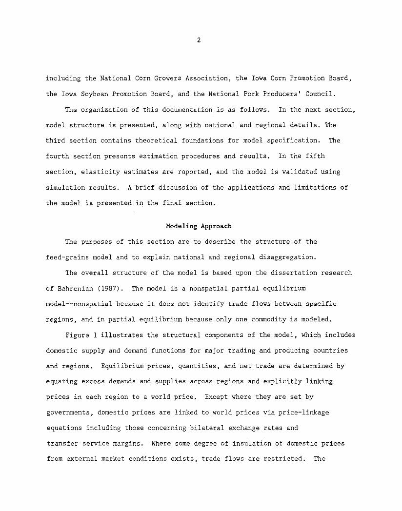
The basic elements of a nonspatial equilibrium supply and demand model are
illustrated in Figure 2. The U.S. export supply curve (ESUS) is the difference
between domestic supply (SUS) and demand (DUS) in the United States and
represents the quantity of exports at various price. levels supplied to the world
market. Other exporters' supply and demand schedules are given in the lower
panel. The curve ESO is the combined excess supply of all competing exporters,
which is the difference between the supply and demand of all exporters. The
import-demand schedule (EDT) of all importers is the difference between total
demand and total supply. Other competitors' export supply and importers' import
demand are represented in the middle diagram of the top panel. The
export-demand schedule (EDN) facing the United States is the difference between
the import demand of all importers and the export supply of all competitors.
The kinked and relatively inelastic nature of the EDN is due to certain foreign
countries' restrictive trade policies, which insulate domestic prices from world
price variability. A trade equilibrium is achieved by the clearing of excess
demands and supplies generated within each region.
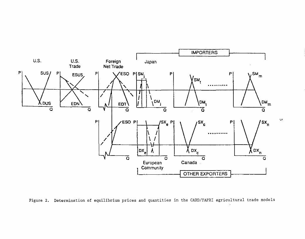
The necessary components of the model are given in the following equations:
m
EDT=~ [FODi(PDi' Xli) + FEDi(PDi' X2i) + SDi(PDi' X3i) - Si(PDi' X4i)], i
i 1, .•. , m importers;
IMPORTERS
u.s. u.s. Foreign Japan Trade Net Trade
p ESUS p ESO p SM. p p
J SM
1 .......... ' ' \
\DMi DM1 DMm
a a a a a
p p sxe p sxc p <.n sxn
\ I .......... \ I
oxe A a a a a
European Canada Community
OTHER EXPORTERS
Figure 2. Determination of equilibrium prices and quantities in the CARD/FAPRI agricultural trade models
ESO
ESUS
ESUS
PD. l
PD. J
where
6
n X (S.(PS., x
4.)- [FOD.(PD., X
1.) + FED.(PD., X
2.) + SD.(PD., x
33.)JJ,
jJJ J JJ J JJ J JJ
j 1, ... , n exporters;
S (P , X4
) - [FOD (P , X1
) +FED (P , X2
) + SD (P , x3u)],
uu u uu u uu u uu
u.s. excess supply;
EON ~ EDT - ESO, world market-equilibrium;
~ G. (P * ei' z.) ' i 1' m importers; and l u ... '
l
G. (P * e.' z.) ' J 1' n exporters; J u • 0 0 '
FOD
FED
SD
s EDT
ESO
ESUS
EDN
PD
PS p u
e
z
~ x4
J J
domestic food demand,
domestic feed demand,
domestic stock demand,
domestic supply,
~ excess-d8mand function of all importers,
~ excess-supply function of all exporters, excluding the United
States,
excess-supply function of the United States,
excess-demand facing the United States,
domestic market price,
~ domestic supply price,
Gulf port price,
exchange rate,
vector of policy variables influencing price transmission,
vector of demand shifters (k ~ 1, •.. , 3), and
~ vector of supply shifters.
The model contains 22 country or regional submodels. The feed-grain
exporters modeled include the United States, Canada, the European Community
(EC), Argentina, Australia, Thailand, China, and South Africa. Importers

7
modeled include the USSR, Japan, Eastern Europe, Brazil, Mexico, Egypt, Saudi
Arabia, India, Nigeria, other Latin American countries, other African and Middle
Eastern countries, high-income East Asia, other Asian countries, and the rest of
the world.
Specification
Theoretical Foundations
This section contains a conceptual model of domestic demand and supply,
which reflects the general structure of the country submodels. Specifications
for individual countries vary significantly, however, particularly for the
United States, Canada, and the European Community. The feed-grain markets of
these countries are modeled in detail by incorporating their respective domestic
policies. The specifications for other countries are, in general, less
detailed.
Domestic Supply Block. The domestic supply block of ith country (exporting
or importing country) is specified as
Area Harvested,
AH. t = AH(PS. t-l'PC. t-l'GP.t,Z. t); l., 1, 1, 1 l,
Production,
PROD it
Supply,
AH. t * YLD. t; and l' l.'
S. t = PROD. t + IM. t + BS. t' l., l, 1, 1,
where area harvested (AH. t) is expressed as a function of the lagged domestic 1,
supply price of feed-grains (PSi t-l)' the lagged domestic price of competing •

8
crops (PC. t-l)' the government policy variable (GP. t), and a vector of other ~' l. J
variables that affect the acreage planted (Zit). Feed-grains production
(PROD. t) is equal to acreage harvested times yield (YLD. t). Finally, 1., l.,
feed-grains supply is equal to production plus imports (IM. t) plus beginning J.,
stocks (BS. t) • J.,
Domestic Demand Block. The conceptual specifications for the domestic
demand block are as follows:
Per Capita Food Demand,
PFOD. t = FOD(PD. t'PY. t); l, l, l,
Total Food Demand,
FOD. t J.,
POP. t * PFOD. t; 1. ' l. '
Feed Demand,
FED. t J.,
FED(PD. t'PS. t,LPI. t,LN.t); and l, l, 1., l.
Ending Stocks,
SD. t J., SD(PD. t,PROD. t,GS. t);
l, l, l.,
where PFOD. t is per capita consumer food demand for feed grains, PY. t is per 1., 1,
capita income, FOD. t is total food demand, FED. t is total feed demand, LPI. t 1, 1., 1.,
is the livestock price index, LN. t is the livestock number, SD. t is ending 1., l,
stocks demand, and GS. t is government stocks. J.,
The detailed theoretical specifications for the U.S feed-grains market are
discussed below.
Acreage response and supply. The estimation of how supply response
will change government commodity programs has been problematic because of
frequent adjustments made in the composition of such programs, as well as the
changes in their underlying payment structures and acreage-reduction options.

9
The most common approach used to incorporate the influence of commodity programs
is to include effective support payment and diversion payment variables as
explanatory variables in the area planted equations (see Houck and Ryan 1972).
As de Gorter and Paddock (1985) note, however, these composite variables ignore
the voluntary nature of the commodity programs and impose questionable
restrictions on the effects of changing policy parameters.
Estimating feed-grains supply response entails the use of endogenous
participation rates. The model's participation rate ([program planted and
idled)/base acreage) is expressed as a function of the difference between
participant expected net returns (PARTENR) and nonparticipant expected net
returns (NPARTENR):
PART f(PARTENR- NPARTENR), (1)
where PART represents the model's participation rate. Increases in participant
expected net returns relative to nonparticipant expected net returns have a
positive effect on program participation.
Participant expected net returns (PARTENR) per acre are derived from
deficiency payments, diversion payments, cash receipts from marketing, and the
variable costs of production and of maintaining idled land. It is assumed that
farmers base program participation and planting decisions on a comparison of
expected net returns under various alternatives. This approach makes it
possible to incorporate a variety of factors that affect producer decisions but
are omitted in models utilizing only market prices or aggregate measures such as
Houck and Ryan's effective support rate. The arithmetic representation of
PARTENR is as follows:

10
PARTENR = max[O, TP- max(LR, LFR)] * PY(l - ARPR- PLDR)
+ DPR * PY * PLDR + max(LR, LFP) * TY(l - ARPR- PLDR)
- VC(l- ARPR- PLDR) - 20(ARPR + PLDR). (2)
The first component of the right-hand side of equation (2) is the expected
deficiency payments. The variables that enter into the expected deficiency
payments are target price (TP), loan rate (LR), lagged farm price (LFP), program
yield (PY) , acreage-reduction program rate (ARPR) , and paid land-diversion rate
(PLDR). The model ARP rate is, in essence, the proportion of base acreage that
all program participants are required to idle to qualify for deficiency
payments. The model PLD rate represents the average proportion of base acreage
idled by program participants to qualify for diversion payments. The second
term is expected diversion payments, where DPR is the diversion payment rate.
The third component is market return, where TY is the trend yield. The fourth
component is the variable cost of production from planted acreage, where VC is
the variable cost of feed-grain production per acre. The final component
indicates that $20 per acre is expected to be spent in maintaining the land
idled under the acreage reduction and the paid land diversion programs.
Nonparticipant expected net returns are defined as
NPARTENR LFP * TY- VC, (3)
where the variables are defined as in the above two equations.
Area planted under programs (APP) is defined as
APP PART(l - ARPR- PLDR) * BA, (4)
where BA is the base average.
ll
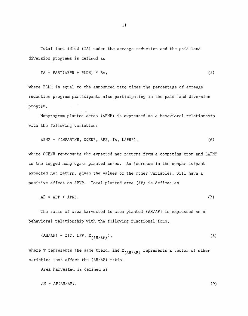
Total land idled (IA) under the acreage reduction and the paid land
diversion programs is defined as
IA = PART(ARPR + PLDR) * BA, (5)
where PLDR is equal to the announced rate times the percentage of acreage
reduction program participants also participating in the paid land diversion
program.
Nonprogram planted acres (APNP) is expressed as a behavioral relationship
with the following variables:
APNP = f(NPARTNR, OCENR, APP, IA, LAPNP), (6)
where OCENR represents the expected net returns from a competing crop and LAPNP
is the lagged nonprogram planted acres. An increase in the nonparticipant
expected net return, given the values of the other variables, will have a
positive effect on APNP. Total planted area CAP) is defined as
AP APP + APNP. (7)
The ratio of area harvested to area planted (AH/AP) is expressed as a
behavioral relationship with the following functional form:
(AH/AP) = f(T, LFP, X(AH/AP)),
where T represents the same trend, and X(AH/AP) represents a vector of other
variables that affect the (AH/AP) ratio.
Area harvested is defined as
AH AP(AH/AP).
(8)
(9)

12
Yield per acre (YD) is expressed as a function of government policy
parameters such as target prices (TP), idled acreage (IA), time trend (T) to
represent technological progress, and other factors (~). Target prices have a
positive effect on yield because higher target prices are assumed to induce
greater input usage. Idled land is assumed to be drawn from less productive
land; therefore, an increase in land idling is expected to increase yields. The
functional form of the yield equation is
YD f(TP, IA, T, ~). (10)
Production (PROD) is defined as the product of acres harvested and yields
per acre:
PROD AH * YD. (11)
Expected net returns are affected significantly by policy parameters.
Therefore, the incorporation of the program-participation decision, which
depends upon expected net returns, into the determination of planted acres
provides a means of analyzing the effects of policy parameter changes on
participation rate, acreage planted, yield, production, and planted area and
production of alternative crops.
Supply is the sum of production, beginning stocks (BI), and exogenous
imports (IM). Thus, the feed-grain supply equation is
s PROD + BI + IM.
Demand
Demand is disaggregated into a number of categories. Major demand
components include food use, feed use, seed use, stocks, and exports.
(12)

13
Domestic Disappearance. The theoretical specification for food use is
based upon the consumer theory of utility maximization subject to budget
constraints. Solution of utility maximization yields consumer demand as a
function of own price, cross prices, and income. Restrictions (homogeneity,
symmetry, Cournot aggregation, and Angel aggregation) derived from demand theory
are not imposed on the estimation, however. The functional form of per capita
food demand (FOOD) is
FOOD (13)
where P represents the own price of the commodity in real terms, P own cross
represents the real price of competing goods, RPCE represents real per capita
consumer expenditure, and Xfood represents a vector of other variables that
explain food use. Total food use is determined as the product of per capita
food use and population.
Because feed is an input into the livestock production equation, the
theoretical specification of feed demand follows the derived demand approach.
Thus, feed demand (FEED) is expressed as a function of the real price of the
commodity (P0wn), the real price of competing feed products (Pcfeed)' livestock
product prices (PL), livestock numbers (LN), and a vector of other variables
Xfeed' Thus, the functional form of feed demand is
FEED= f(Pown' pcfeed' PL, LN, Xfeed). (14)
The demand for seed use (SEED) is specified as a function of acreage
planted (AP) and a time trend (T). The behavioral relationship is written as
SEED f (AP, T) . (15)

14
Stocks. Total inventories (EI) are further disaggregated into Commodity
Credit Corporation (CCC) inventories, Farmer-Owned Reserve (FOR) stocks,
nine-month-loan-program carryover, and "free" stocks unencumbered by government
programs. Commodity Credit Corporation, FOR, and nine-month-loan stocks are
exogenous in the model; however, in policy analyses these stocks are adjusted to
reflect factors ranging from loan rates and market prices to participation rates
and the availability of generic certificates.
Free (or private) stocks are endogenized in the model by using speculative
and transactional motives of inventory demand theory. The speculative motive
indicates that the amount of grain stored at any time depends upon the
difference between current and expected prices. According to the theory of
stock demand, this price difference must be equated to the marginal cost of
storage to determine the optimal level of storage. It is assumed further that
commercial stockholders base their expectation regarding future prices upon
expected production and government stocks. The transaction motive indicates
that the amount of grain stored is determined by the level of current output.
Using these two motives for storage, the behavioral relationships for free
stocks (STOCK) are specified as
STOCK f(Pown' PROD, EPROD, GSTOCK, XSTOCK), (16)
where PROD is current production, EPROD is expected production, GSTOCK is
government stock (the sum of CCC, FOR, and nine-month-loan stocks), and XSTOCK
is a vector of other variables that influence free stocks.
Exports. Feed-grain exports are determined as residuals:
EX PROD + BI + IM- FOOD - FEED - SEED - EI.

15
The above specification of demand is based upon a price theory that may not
be applicable to the centrally planned economies of the Soviet Union, China, and
Eastern Europe, or indeed to most other developing countries. For these
regions, demand is postulated to depend upon income and available supplies which
are derived mainly from production. That is,
(17)
A linear specification of this demand function is
(18)
Import demand as a residual of demand and supply becomes
Data Sources
The data used for the analyses include feed-grain use and supply-quantity
data obtained from the Foreign Agricultural Service of the USDA. Macroeconomic
data such as income, exchange rates, and inflation are obtained from the
International Monetary Fund (IMF). All macroeconomic data have been converted
to the appropriate crop-year basis for each country or regional component. For
example, a calendar-year macrovariable is converted to an October-September
crop-year basis by taking a weighted average of its October to December values
for the first year and of its January to September values for the second year.
Weights are 0.25 for the first three months and 0.75 for the second nine months.
Most feed-grain price data were derived from Food and Agricultural Organization
(FAO) price statistics. Additional price information regarding the United

16
States, Canada, Australia, and the European Community was obtained from USDA
Agricultural Statistics (various years), Canada Grain Trade Statistics (various
years), Yearbook of the Commonwealth of Australia (various years), and The
Agricultural Situation in the Community (various years).
Empirical Results
This section presents estimation procedures, estimated equations, and
identities. Reasons for the inclusion of relevant variables in an equation,
along with the sign and the significance of the estimated coefficients, are
discussed. The equations reported here reflect the state of the model as of
summer 1989.
Most of the equations in the model are estimated using annual data from the
period 1965/66-1986/87 (or shorter intervals if data were unavailable at the
time of estimation).
All equations are estimated using ordinary least squares (OLS) utilizing
AREMOS, an econometric package developed by The WEFA Group. Given the
simultaneity of the model and the nonlinearity of many of the modeled
relationships, OLS is not the most appropriate estimation technique from a
theoretical standpoint. OLS does, however, make it easy to replace
unsatisfactory equations, an important strength for a model that is constantly
undergoing revision. Future revisions of the model will utilize more
appropriate estimation techniques.
For each estimated equation, t-statistics are presented in parentheses
below the parameter estimates. Where appropriate, elasticities evaluated at the
mean of all variables are reported in brackets. Also reported for each
estimated equation are the estimation period, the R-squared, the adjusted

17
R-squared, the standard error of estimates, the Durbin-Watson statistic, and the
mean of the dependent variable.
United States Submodel
The U.S. component of the feed-grains model is illustrated in Table 1.
Estimated equations are reported in the following order: corn, sorghum, barley,
and oats. The estimated results are satisfactory, with anticipated signs and
generally high R-square values, The supply side is modeled by estimating
participation rate and nonparticipant acreage. Total area planted is equal to
nonparticipant planted area plus participant planted area. Participant planted
area is equal to the participation rate times the base area times the percentage
of base acres that participants can plant. Acreage harvested as a percentage of
acreage planted is determined endogenously. Yield is also determined
endogenously. Production is determined as area harvested times yield.
The expected participation rate for corn (Eq. 1.1) is estimated as a
function of expected participant net returns minus a weighted average of
nonparticipant expected net returns and soybean expected net returns and a
series of dummy variables for years with no government land-idling programs.
The positive coefficients for the variable--the difference between participant
net returns and the weighted average of nonparticipant and soybean net
returns--indicate that more farmers will participate in the government program
if program benefits are greater.
The participant, nonparticipant, and soybean expected net returns are given
by identities 1.2, 1.3, and 1.4, respectively. The nonparticipant corn acreage
in the next year (1.5) is estimated as a function of area planted by
participants, corn acreage idled under ARP, PLD programs plus CRP acres,

18
Table 1. Structural parameter estimates of the U.S. feed-grains submodel
Corn
(1.1) Corn Program Participation Rate (Next Year)
COMPRU9F = 0.561 + 0.770[CONRPU9F- (0.8 CONRNU9F (14.04) (2.59)
+ 0.2 SBNRNU9F)]/PWSAU9 - 0.594 DM173 - 0.6 DM174 (3.83) (3.86)
- 0.615 DM175 - 0.535 DM176 - 0.559 DM179 - 0.568 DM180 (3.89) (3.45) (3.62) (3.67)
DW = 1. 65
(1.2) Participants Corn Expected Net Return
CONRPU9F = [Max(COPTGU9F- Max (COPLNU9F, COPFMU9), 0]
* COYHPU9F(1 - COMARU9F - COMPLU9F) + CODPRU9F * COYHPU9F
* COMPLU9F + MAX(COPLNU9F, COPFMU9)
* COYHTU9F(1 - COMARU9F - COMPLU9F) - COVCAU9F(1 - COMARU9F
- COMPLU9F) - 20(COMARU9F + COMPLU9F)
(1.3) Nonparticipants Corn Expected Net Return
CONRNU9F = COPFMU9 * COYHTU9F - COVCAU9F
(1.4) Soybeans Expected Net Return
SBNRNU9F = SBPFMU9 * SBYHTU9F - SBVCAU9F
(1.5) Corn Nonprogram Acreage (Next Year)
COAPNU9F = 82.741- 0.963 (38.99) (48.13)
[ -0. 43]
COAPPU9F- 0.743(COAIAU9F + COCRPU9F) (22.31)
+ 5.050 (2.04) [0.05]
CONRNU9F/PWSAU9 - 2.814 (0.78)
[-0.03]
[-0.15]
SBNRNU9F/PWSAU9

Table 1. Continued
- 7.830 DM17274 (6.23)
R2 = 1.00 DW = 2.40
19
(1.6) Corn Program Acreage (Next Year)
COAPPU9F = COMPRU9F * COABAU9F(1 - COMARU9F - COMPLU9F)
(1.7) Total Corn Area Planted (Next Year)
COAPAU9F = COAPPU9F + COAPNU9F
(1.8) Corn Area Harvested as a Proportion of Area Planted (Next Year)
COAHPU9F = 0.800 - 0.043 DM182 + 0.020 LOG(TREND-1959) (28.75) (3.70) (1.90)
+ 0.010 DMCOYU9F + 0.030 DM1S77 (1.80) (4.10)
+ 0.034(COAIAU9F + COCRPU9F)/COAPAU9F (2.40) [0.01]
R2 = 0. 900 DW = 2.32
(1.9) Corn Area Idled
COAIAU9F = COABAU9F * COMPRU9F(COMARU9F + COMPLU9F)
(1.10) Total Corn Area Harvested
COAHAU9F = COAPAU9F * COAHPU9F
(1.11) Corn Yield (Next Year)
COYHAU9F = 211.400 + 2134.020 COPTGU9F/PWSAU9 (5.20) (1.46)
[0.23)

20
Table 1. Continued
+ 83.272 LOG(TREND - 1945) (9.46)
+ 0.092 COAIAU9F + COCRPU9F (0.50)
[0.01)
+ 10.604 DMCOYU9F - 20.804 DM182 (3.95) (2.63)
R2 0.92 DW = 2.35
(1.12) Corn Production (Next Year)
COSPRU9F = COAHAU9F * COYHAU9F
(1.13) Corn Feed Use
COUFEU9G = 40,505- 1749.760 COPFMU9/PWSAU9 (3.20) (5.91)
[ -0. 29)
+ 2374.48 LVPIU9/PWSAU9 ( 2. 04) [ 0. 29)
- 0.430(WHUFEU9 (2.22)
[-0.14)
* 60/56 + SGUFEU9
+ BAUFEU9 * 48/56 + OAUFEU9 * 32/56)/GCAUU9
+ 10.230 LOG(TREND - 1959) (4.13)
+ 4.941 SMPFMU9/PWSAU9 ( 1. 28) [0.06)
+ 14.430 DM173 - 6.735 DM176 (4. 72) (3.46)
R2 0. 89 DW = 3,08
(1.14) Total Corn Feed Use
COUFEU9 = COUFEU9G * GCAUU9
(1.15) Corn Food Use
COUOFU9C = 5.900- 0.337 COPFMU9/(WHPFMU9/2.763 + SUPRTU9/25.805) (10.40) (2.12)
[-0.14)

21
Table 1. Continued
+ 4.071 LOG(CESAU9/DEPOPU9) (16.82)
R2 = 0.99
(1.59)
- 2.530 DM1S83 LOG(CESAU9/DEPOPU9) + 0.345 DM1S80 (1.85) (5.88)
[-0.99]
+ 5.900 DM1S83 (1. 89)
DW = 1. 80
(1.16) Total Corn Food Use
COUOFU9 = COUOFU9 * DEPOPU9
(1.17 Corn Gasohol Use
COUGAU9 = 0.000- 4772.700 DM1S80 * COPFMU9/PWFSAU9 (0.00) (2.67)
[-0.11]
+ 602.730 DM1S79 * LOG(TREND- 1965) (8.12)
- 1580.690 DM1S79 + 12.871 TRND8184 (8.01) (2.20)
R2 = 0.99 DW = 2.76
(1.18) Corn Seed Use
COUSDU9 = 296.314 + 0.280 COAPAU9F + 0.150 TREND (5.51) (13.88) (5.40)
[ 1. 20]
DW=1.72
(1.19) Total Corn Domestic Use
COUTOU9 = COUFEU9G + COUOFU9 + COUGAU9 + COUSDU9

Table 1. Continued
(1.20) Corn Free Stocks
COFREU9 = 465.703 (1.47)
22
- 31056.000 COPMFU9/PWSAU9 (1. 89)
[-1.64]
- 0.053 (1. 74)
[-0.66]
+ 0.147 (3.92) [ 1. 83]
LAG(COSPRU9F) + 231.238 DM1S75 (2.12)
- 0.313(C09LNU9 + COCCCU9 + COFORU9) (7.46)
[-0.68]
DW = 1.94
(1.21) Corn Total Stocks
COCOTU9 = COFREU9 + C09LNU9 + COFORU9 + COCCCU9
(1.22) Corn Gulf-Port Price
COPOBU9 = 1.0913 CORPF * 39.368 + 5.8374
(1.23) Corn Domestic Market Equilibrium
COSPRU9F
COSPRV9 + LAG(COCOTU9) + COSMTU9 COUFEU9 + COUFOU9 + COUXTU9
+ COCOTU9 + COURSU9
Sorghum
(1.24) Sorghum Participation Rate
SGMPRU9 = 26.685 + 1.153(SGENRPU9 - SGNRNU9)/PWSAU9 - 0,013 TREND (1.68) (1.87) (1.65)
+ 0.314 DM172 - 0.600 DM174 - 0.586 DM175 (2.41) (4.62) (4.55)
- 0.573 DM176 - 0.635 DM177 - 0.554 DM180 (4.47) (4.78) (4.31)

Table 1. Continued
- 0.507 DM181 (3.82)
R2 = 0.91 DW = 1.67
(1.25) Sorghum Participant Net Return
23
SGNRPU9 = max(SGPTGU9 - max[SGPLNU9, LAG(SGPFMU9)] ,0)
* SGYHPU9(1 - SGMARU9 - SGMPLU9) + SGDPRU9 * SGYHPU9 * SGMPLU9
+ max[SGPLNU9, LAG(SGPFMU9)) * SGYHTU9(1 - SGMARU9
- SGMPLU9) - SGVCAU9(1 - SGMARU9 - SGMPLU9)
- 20(SGMARU9 + SGMPLU9)
(1.26) Wheat Net Return
WHNRNU9 = LAG(WHPFMU9) * WHYHTU9 - WHVCAU9
(1.27) Sorghum Nonparticipant Net Returns
SGNRNU9F = SGPFMU9 * SGYHTU9F - SGVCAU9F
(1.28) Sorghum Area Planted by Participants
SGAPPU9 = SGMPRU9 * SGABAU9(1 - SGMARU9 - SGMPLU9)
(1.29) Sorghum Area Planted by Nonparticipants
SGAPNU9 = 19.783 + 8,691 SGNRNU9/PWSAU9 (20.03) (3.42)
[0. 20)
- 1.096 WHNRNU9/PWSAU9 (0.43)
[-0.02)
- 0.868 (17.89) [-0.47)
SGAPPU9 - 0.747 (8.66)
[-0.19)
SGAIAU9 + SGCRPU9
- 5.557 DM1S74- 2.851 DM173 + 2.070 DM185 (11.07) (4.09) (3.53)
DW = 2.35

24
Table 1. Continued
(1.30) Sorghum Area Idled under the ARP and PLD Programs
SGAIAU9 = SGABAU9 * SGMPRU9(SGMARU9 + SGMPLU9)
(1.31) Sorghum Total Area Planted
SGAPAU9 = SGAPPU9 + SGAPNU9
(1.32) Sorghum Area Harvested as a Proportion of Area Planted
SGAHPU9 = 0.544 + 0.023 DMSGYU9 + 0.103 LOG(TREND- 1959) (13.62) (2.34) (7.34)
R2 = 0.76 DW = 1.56
(1.33) Sorghum Total Area Harvested
SGAHAU9 = SGAPAU9 * SGAHPU9
(1.34) Sorghum Yield
SGYHAU9 = 1369.810 + 0.171 TREND+ (4.33) (4.56)
+ 8.422 DMSGYU9 (4.95)
DW = 2.64
(1.35) Sorghum Production
SGSPRU9 = SGAHAU9 * SGYHAU9
(1.36) Sorghum Feed Use
806.744 (0.95) [0.14]
SGPTGU9/PWSAU9
SGUFEU9 = 568.311 - 115318.000 SGPFMU9/PWSAU9 (2.43) (2.59)
[-2.08]

25
Table 1. Continued
+ 60406.300 COPFMU9/PWSAU9 + (1.50)
17993.500 WHPFMU9/PWSAU9 (1.67)
[1.21] [0.47]
+ 38.731 CATNFU9- 15,952 TRN06783 (1.68) (3,98) [0.65]
R2 0. 66 ow = 1. 64
(1.37) Sorghum Food, Seed, and Industrial Use
SGUFOU9 14.803- 1857.54 SGPFMU9/PWSAU9 (7.84) (1.30)
[-1.42]
+ 949.118 BAPFMU9/PWSAU9 ( 1. 48) [0. 71]
+ 14.652 DM185 (6.61)
R2 0.81 ow = 2.04
+ 567,415 (0.57) [0. 48]
(1.38) Sorghum Free and Nine-Month Loan Stocks
SGF9LU9 = 51.677 + 0,395 LAG(SGF9LU9) -(0.39) (2.02)
R2 0. 60
+ 0.230 SGSPRU9 (2.30) [1.97]
ow = 1. 70
(1.39) Sorghum Total Stocks
- 0,234(SGCCCU9 (2. 01)
[-0.38]
SGCOTU9 = SGCCCU9 + SGFORU9 + SGF9LU9
(1.40) Sorghum Price Linkage Equation
SGPOBU9 = 5.90457 + 44.7348 SORPF
COPFMU9/PWSAU9
14294.5 SGPFMU9/PWSAU9 (1.92)
[-1.51]
+ SGFORU9)

26
Table 1. Continued
(1.41) Sorghum Domestic Market Equilibrium
SGSPRU9 + LAG(SGCOTU9) + SGSMTU9 SGUFEU9 + SGUFOU9 + SGUXNU9
+ SGCOTU9
(1.42) World Market Equilibrium
SGUXNU9 SGSMNAR + SGSMNAU + SGSMNZA + SGSMNMX + SGSMNNG
+ SGSMNIN + SGSMNROW + SGSTDIS
Barley
(1.43) Barley Participation Rate
BAMPRU9 = 1.990 + 3.455(BANRPU9 - BANRNU9)/PWJMU9 (2.45) (3.08)
- 0.825 DM171- 0,720 DM174- 0.689 DM175- 0.661 DM176 (4.57) (4.68) (4.65) (4.57)
- 0.634 DM177- 0.733 DM180- 0.540 DM181 (4.47) (4.94) (3.80)
- 0.469 LOG(TREND - 1959) (2.08)
DW = 1.75
(1.44) Barley Participant Net Returns
BANRPU9 = max(BAPTGU9 - max[BAPLNU9, LAG(BAPFMU9)], 0}
* BAYHPU9(1 - BAMARU9 - BAMPLU9) + BADPRU9 * BAYHPU9 * BAMPLU9
+ MAX[BAPLNU9, LAG(BAPFMU9) * BAYHTU9(1 - BAMARU9 - BAMPLU9]
- BAVCAU9(1 - BAMARU9 - BAMPLU9)
- 20(BAMARU9 + BAMPLU9)
(1.45) Barley Nonparticipant Net Returns
BANRNU9F = BAPFMU9 * BAYHTU9F - BAVCAU9F

27
Table 1. Continued
(1.46) Barley Area Planted by Participants
BAAPPU9 = BAMPRU9 * BAABAU9(1 - BAMARU9 - BAMPLU9)
(1.47) Barley Area Planted by Nonparticipants
BAAPNU9 = 10.303 + ( 15. 20)
12.083 (1. 68) [0.35]
BANRNU9/PWJMU9 - 0.908 BAAPPU9 (10.95) [-0.39]
- 0.553·DM1S74(BAAIAU9 + BACRPU9)+ 2.706 DM1S84 (2.07) (4.27)
[-0.04]
- 411.320 (WHNRNU9/49 + OANRNU9/27 * 0.5)/PWJMU9 ( 1. 86)
[-0.42]
DW = 1. 40
(1.48) Barley Area Idled under the ARP and PLD Programs
BAAIAU9 = BAABAU9 * BAMPRU9(BAMARU9 + BAMPLU9)
(1.49) Barley Total Area Planted
BAAPAU9 = BAAPPU9 + BAAPNU9
(1.50) Barley Area Harvested as a Proportion of Area Planted
BAAHPU9 = 0.917 - 0,037 DM180 + 0.035 DM18183 - 0.038 DM185 (301.61) (2.98) (4.53) (3.04)
DW = 1.67
(1.51) Barley Total Area Harvested
BAAHAU9 = BAAPAU9 * BAAHPU9
(1.52) Barley Yield
BAYHAU9 = -1528.970 + 0.795 TREND+ 4.504 DMBAYU9 (9.48) (9. 76) (5.21)

28
Table l. Continued
+ 424.511 BAPTGU9/PWJMU9 + 2.653 DM171 (1.03) (0.60) [0.07]
DW = 2.15
(1.53) Barley Production
BASPRU9 = BAAHAU9 * BAYHAU9
(1,54) Barley Feed Use
BAUFEU9 120.627 + 0.638 LAG(BAUFEU9)
- 16246,500 BAPFMU9/PWJMU9 (2.93)
[-0.66]
+ 9325.640 (2.31) [0.43]
COPFMU9/PWJMU9
+ 1068.560 WHPFMc9/PWJMU9 + 31.705 DM18285 (0.39) (2.85) [0. 06]
DW = 2.32
(1.55) Barley Per Capita Food, Seed, and Industrial Use
BAUFOU9C = 0.243 - 1.234 BAPFMU9/PWJMU9 (2.97) (1.20)
+ 0.220 (5.30) [0.31]
[ -0 .02]
LOG(CEJMU9/DEPOPU9) + 0.049 DM1S78 (6.06)
- 0.017 TRND8185 (8.15)
DW = 2.16
(1.56) Barley Total Food, Seed, and Industrial Use
BAUFOU9 = BAUFOU9C * DEPOPU9

29
Table 1. Continued
(1.57) Barley Free and Nine-Month Loan Stocks
BAF9LU9 = 72.526 + 0.349 LAG(BAF9LU9) -(0.69) (2.10)
+ 0.300 BASPRU9 (1.72) [0.89]
- 48.099 DM18183 ( 3 . 04)
DW = 2.12
(1.58) Barley Total Stocks
- 0.632(BACCCU9 (2.94)
[-0.20]
BACOTU9 = BAF9LU9 + BACCCU9 + BAFORU9
(1.59) Barley Exports
7600.720 BAPFMU9/PWJMU9 (2.43)
[-0.48]
+ BAFORU9)
BAUXTU9 = -200 BAPFMU9 + 100 COPFMU9 + 40 WHPFMU9 + BAUXEU9
(1.60) Barley Domestic Market Equilibrium
BASPRU9 + LAG(BACOTU9) + BASMTU9 = BAUFOU9 + BAUFEU9 + BAUXTU9
+ BACTOU9 + BAURSU9
Oats
(1.61) Oats Participation Rate
OAMPRU9 = 0.000 + 5.215(0ANRPU9 - OANRNU9)/PWJMU9 * DMlS82 (0.00) (4.96)
+ 0.202 DMlS82 ( 9. 00)
DW = 2.22

30
Table 1. Continued
(1.62) Oats Participant Net Returns
OANRPU9 = max(OAPTGU9 - max[OAPLNU9, LAG(OAPFMU9)], 0}
* OAYHPU9(1 - OAMARU9 - OAMPLU9) + OADPRU9 * OAYHPU9 * OAMPLU9
+ max[OAPLNU9, LAG(OAPFMU9)] * OAYHTU9(1 - OAMARU9 - OAMPLU9)
- OAVCAU9(1 - OAMARU9 - OAMPLU9)
- 20(0AMARU9 + OAMPLU9)
(1.63) Oats Nonparticipant Net Returns
OANRNU9F = OAPFMU9 * OAYHTU9 - OAVCAU9
(1. 64) Oats Area Planted by Participants
OAAPPU9 = OAMPRU9 * OAABAU9(1 - OAMARU9 - OAMPLU9)
(1.65) Oats Area Idled under the ARP and PLD Programs
OAAIAU9 = OAABAU9 * OAMPRU9(0AMARU9 + OAMPLU9)
(1.66) Oats Area Planted by Nonparticipants
OAAPNU9 = OAAPAU9 - OAAPPU9
(1.67) Oats Total Area Planted
OAAPAU9 = 7.783 + 0.666 OAAHAU9 (10.08) (9.64)
[0.47]
R2 0.95 DW = 1.35
(1.68) Oats Total Area Harvested
+ 0.164 COAIAU9- 6.283 DM183 (6.58) (5.73) [0 0 10]
OAAHAU9 = 13.560 + 0.195 LAG(OAAHAU9) + 18.835 OANRNU9/PWJMU9 (3.22) (0.87) (2. 76)
[0.22]

31
Table 1. Continued
(1.69)
(1. 70)
- 0.480 OAAIAU9 + OACRPU9 - 0.434 TRND7186 (0.84) (2.95)
[-0.01]
- 230.106(CONRNU9/101 + SBNRNU9/96 + BANRNU9/43)/PWJMU9 (2.75)
[-0.26]
R2 0.95 DW = l. 99
Oats Yield
OAYHAU9 -938.112 + 0.501 TREND + 5.270 DMOAYU9 (6.74) (7 .12) (7.11)
R2 0.81 DW = 2.91
Oats Production
OASPRU9 = OAAHAU9 * OAYHAU9
(1.71) Oats Feed Use
OAUFEU9 = 868,822- 49237,300 OAPFMU9/PWJMU9 (37,90) (8.91)
[-0.52]
+ 14173.500 COPFMU9/PWJMU9 (5.25)
- 21.787 TRND7186 - 65.391 DM17780 (24.15) (6.41)
[0. 27]
R2 0. 98 DW = 2.47
(1.72) Oats Per capita Food, Seed, and Industrial Use
OAUFOU9C = 1.116- 2.920 OAPFMU9/PWJMU9 (5.34) (0.91)
[-0.04]
- 0.376 LOG(CEJMU9/DEPOPU9) (4. 71)
[-0.95]
DW = 1. 86
+ 1.224 OAAPAU9F/DEPOPU9 (3.27) [0.24]
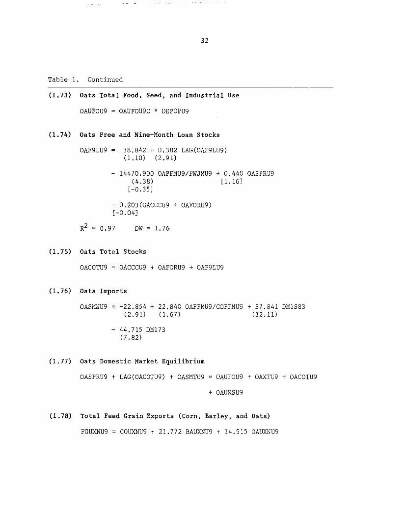
32
Table 1. Continued
(1.73) Oats Total Food, Seed, and Industrial Use
OAUFOU9 = OAUFOU9C * DEPOPU9
(1.74) Oats Free and Nine-Month Loan Stocks
OAF9LU9 = -38.842 + 0.382 LAG(OAF9LU9) (1.10) (2.91)
- 14470.900 OAPFMU9/PWJMU9 + 0.440 OASPRU9 (4.38) [1.16]
[-0.35]
- 0.203(0ACCCU9 + OAFORU9) [-0.04]
DW = 1. 76
(1.75) Oats Total Stocks
OACOTU9 = OACCCU9 + OAFORU9 + OAF9LU9
(1.76) Oats Imports
OASMNU9 = -22.854 + 22.840 OAPFMU9/COPFMU9 + 37.841 DM1S83 (2.91) (1.67) (12.11)
- 44.715 DM173 (7.82)
(1.77) Oats Domestic Market Equilibrium
OASPRU9 + LAG(OACOTU9) + OASMTU9 OAUFOU9 + OAXTU9 + OACOTU9
+ OAURSU9
(1.78) Total Feed Grain Exports (Corn, Barley, and Oats)
FGUXNU9 = COUXNU9 + 21.772 BAUXNU9 + 14.515 OAUXNU9
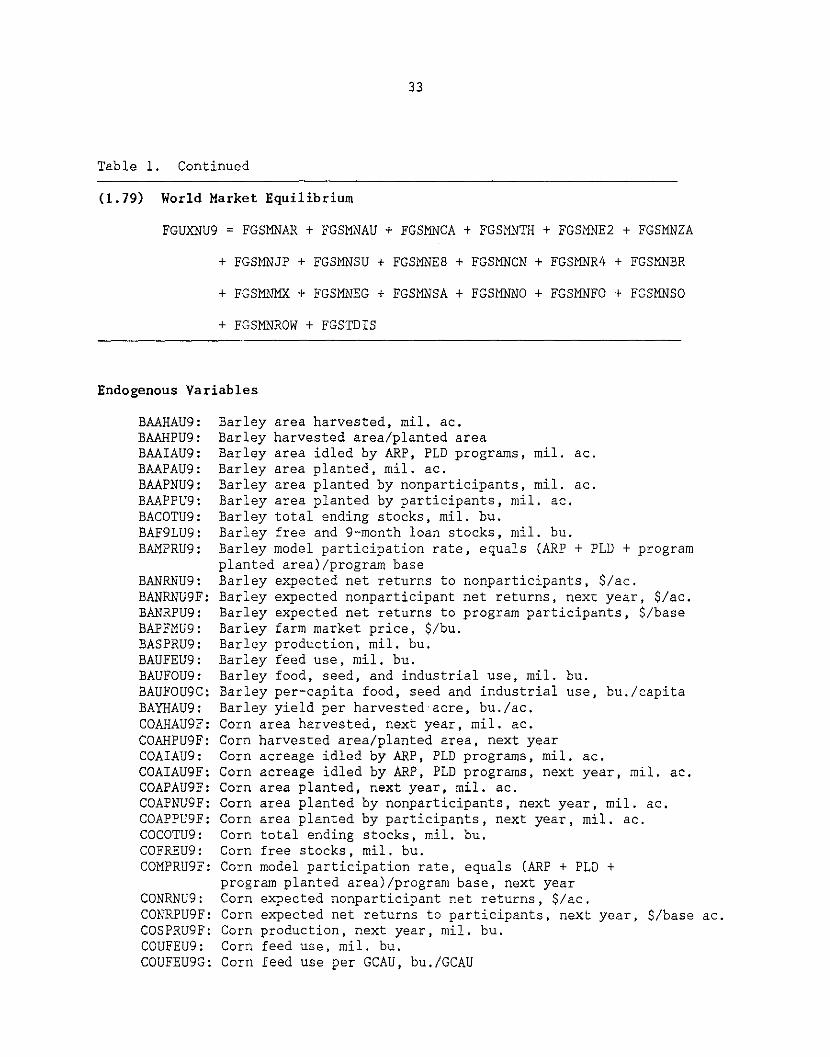
33
Table l. Continued
(1.79) World Market Equilibrium
FGUXNU9 = FGSMNAR + FGSMNAU + FGSMNCA + FGSMNTH + FGSMNE2 + FGSMNZA
+ FGSMNJP + FGSMNSU + FGSMNEB + FGSMNCN + FGSMNR4 + FGSMNBR
+ FGSMNMX + FGSMNEG + FGSMNSA + FGSMNNO + FGSMNFO + FGSMNSO
+ FGSMNROW + FGSTDIS
Endogenous Variables
BAAHAU9: BAAHPU9: BAAIAU9: BAAPAU9: BAAPNU9: BAAPPU9: BACOTU9: BAF9LU9: BAMPRU9:
BANRNU9: BANRNU9F: BANRPU9: BAPFMU9: BASPRU9: BAUFEU9: BAUFOU9: BAUFOU9C: BAYHAU9: COAHAU9F: COAHPU9F: COAIAU9: COAIAU9F: COAPAU9F: COAPNU9F: COAPPU9F: COCOTU9: COFREU9: COMPRU9F:
CONRNU9: CONRPU9F: COSPRU9F: COUFEU9: COUFEU9G:
Barley area harvested, mil. ac. Barley harvested area/planted area Barley area idled by ARP, PLD programs, mil. ac. Barley area planted, mil. ac. Barley area planted by nonparticipants, mil. ac. Barley area planted by participants, mil. ac. Barley total ending stocks, mil. bu. Barley free and 9-month loan stocks, mil. bu. Barley model participation rate, equals (ARP + PLD +program planted areal/program base Barley expected net returns to nonparticipants, $/ac. Barley expected nonparticipant net returns, next year, $/ac. Barley expected net returns to program participants, $/base Barley farm market price, $/bu. Barley production, mil. bu. Barley feed use, mil. bu. Barley food, seed, and industrial use, mil. bu. Barley per-capita food, seed and industrial use, bu./capita Barley yield per harvested acre, bu./ac. Corn area harvested, next year, mil. ac. Corn harvested area/planted area, next year Corn acreage idled by ARP, PLD programs, mil. ac. Corn acreage idled by ARP, PLD programs, next year, mil. ac. Corn area planted, next year, mil. ac. Corn area planted by nonparticipants, next year, mil. ac. Corn area planted by participants, next year, mil. ac. Corn total ending stocks, mil. bu. Corn free stocks, mil. bu. Corn model participation rate, equals (ARP + PLD + program planted areal/program base, next year Corn expected nonparticipant net returns, $/ac. Corn expected net returns to participants, next year, $/base ac. Corn production, next year, mil. bu. Corn feed use, mil. bu. Corn feed use per GCAU, bu,/GCAU
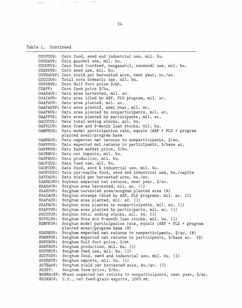
34
Table l. Continued
COUFOU9: COUGAU9: COUOFU9: COUSDU9: COYHAU9F: COUTOU9: COPOBU9: CORPF: OAAHAU9: OAAIAU9: OAAPAU9: OAAPAU9F: OAAPNU9: OAAPPU9: OACOTU9: OAF9LU9: OAMPRU9:
OANRNU9: OANRPU9: OAPFMU9: OASMNU9: OASPRU9: OAUFEU9: OAUFOU9: OAUFOU9C: OAYHAU9: SBNRNU9F: SGAHAU9: SGAHPU9: SGAIAU9: SGAPAU9: SGAPNU9: SGAPPU9: SGCOTU9: SGF9LU9: SGMPRU9:
SGNRNU9: SGNRPU9: SGPOBU9: SGSPRU9: SGUFEU9: SGUFOU9: SGUXNU9: SGYHAU9: SORPF: WHNRNU9F: FGUXNU9:
Corn food, seed and industrial use, mil. bu. Corn gasohol use, mil. bu. Corn food (nonfeed, nongasohol, nonseedl use, mil. bu. Corn seed use, mil. bu. Corn yield per harvested acre, next year, bu./ac. Total corn domestic use, mil. bu. Corn Gulf Port price $/mt. Corn farm price $/bu. Oats area harvested, mil. ac. Oats area idled by ARP, PLD program, mil. ac. Oats area planted, mil. ac. Oats area planted, next year, mil. ac. Oats area planted by nonparticipants, mil. ac. Oats area planted by participants, mil. ac. Oats total ending stocks, mil. bu. Oats free and 9-month loan stocks, mil. bu. Oats model participation rate, equals (ARP + PLD + program planted areal/program base Oats expected net =eturns to nonparticipants, $/ac. Oats expected net returns to participants, $/base ac. Oats farm market price, $/bu. Oats net imports, mil. bu. Oats production, mil. bu. Oats f.eed use, mil. bu. Oats food, seed & industrial use, mil. bu. Oats per-capita food, seed and industrial use, bu./capita Oats yield per harvested acre, bu./ac. Soybean expected net returns, next year, $/ac. Sorghum area harvested, mil. ac. (1l Sorghum harvested area/sorghum planted area (8l Sorghum acreage idled by ARP, PLD programs, mil. ac. (1) Sorghum area planted, mil. ac. (1l Sorghum area planted by nonparticipants, mil. ac. (1l Sorghum area planted by participants, mil. ac. (1l Sorghum total ending stocks, mil. bu. (1l Sorghum free and 9-month loan stocks, mil. bu. (1l Sorghum model participation rate, equals CARP+ PLD +program planted areal/program base (8l Sorghum expected net returns to nonparticipants, $/ac. (8l Sorghum expected net returns to participants, $/base ac. (8l Sorghum Gulf Port price, $/mt Sorghum production, mil. bu. (1l Sorghum feed use, mil. bu. (1l Sorghum food, seed and industrial use, mil. bu. (1l Sorghum exports, mil. bu. (1l Sorghum yield per harvested acre, bu./ac. (1l Sorghum farm price, $/bu. Wheat expected net returns to nonparticipants, next year, $/ac. U.S., net feed-grain exports, 1000 mt.

35
Table 1. Continued
FGSMNAR: FGSMNAU: FGSMNTH: FGSMNE2: FGSMNZA: FGSMNJP: FGSMNSU: FGSMNE8: FGSMNCN: FGSMNR4: FGSMNBR: FGSMNMX: FGSMNEG: FGSMNSA: FGSMNNO: FGSNFFO: FGSMNSO: FGSMNROW: SGSMNAR: SGSMNAU: SGSMNZA: SGSMNMX: SGSMNNG: SGSMNIN: SGUXNU9: SGSMNROW:
Argentina, feed-grain imports, 1000 mt. Argentina, feed-grain imports, 1000 mt. Thailand, feed-grain imports, 1000 mt. EC, feed-grain imports, 1000 mt. South Africa, feed-grain imports, 1000 mt. Japan, feed-grain imports, 1000 mt. Soviet Union, feed-grain imports, 1000 mt. Eastern Europe, feed-grain imports, 1000 mt. China, feed-grain imports, 1000 mt. High Income East Asia, feed-grain imports, 1000 mt. Brazil, feed-grain imports, 1000 mt. Mexico, feed-grain imports, 1000 mt. Egypt, feed-grain imports, 1000 mt. Saudi Arabia, feed-grain imports, 1000 mt. Other Latin America, feed-grain imports, 1000 mt. Other Africa and Middle East, feed-grain imports, 1000 mt. Other Asia, feed-grain imports, 1000 mt. Rest of the World, feed-grain imports, 1000 mt. Argentina, sorghum imports, 1000 mt. Australia, sorghum imports, 1000 mt. South Africa, sorghum imports, 1000 mt. Mexico, sorghum imports, 1000 mt. Nigeria, sorghum imports, 1000 mt. India, sorghum imports, 1000 mt. U.S., sorghum exports, 1000 mt. ROW, sorghum imports, 1000 mt.
Exogenous Variables
BAABAU9: BACCCU9: BACRPU9: BADPRU9: BAFORU9: BAMARU9:
BAMPLU9:
BAPLNU9: BAPTGU9: BASMTU9: BAURSU9: BAUXTU9: BAVCAU9:
BAVCAU9F: BAYHPU9: BAYHTU9:
Barley program acreage base, mil. ac. Barley CCC stocks, mil. bu. Barley program base enrolled in the CRP, mil. ac. Barley diversion payment rate, $/bu. Barley FOR stocks, mil. bu. Barley model ARP rate, equals ARP area/CARP + PLD + program planted area) Barley model PLD rate, equals PLD area/CARP + PLD + program planted area) Barley loan rate, $/bu. Barley target price, $/bu. Barley imports, mil. bu. Barley statistical discrepancy, mil. bu. Barley exports, mil. bu. Barley variable production costs--includes family labor and interest on variable expenses, $/ac. Barley variable production costs, next year, $/ac. Barley program yield, bu./ac. Barley trend yield, bu./ac.
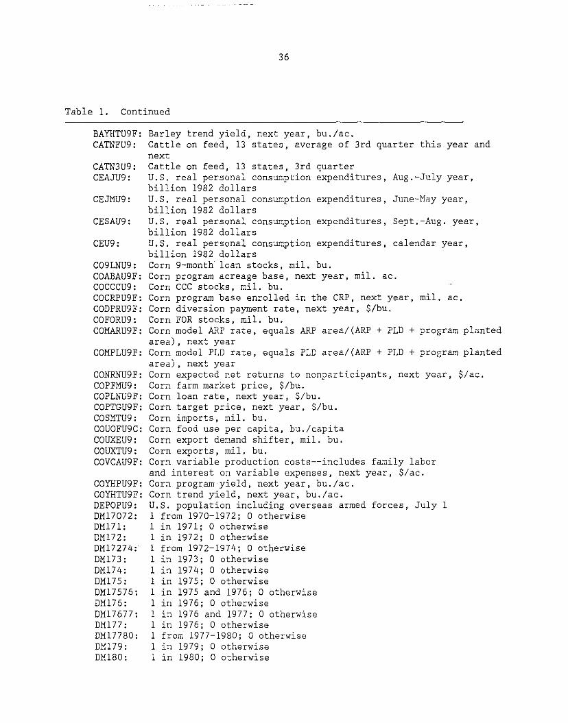
36
Table 1. Continued
BAYHTU9F: Barley trend yield, next year, bu./ac. CATNFU9: Cattle on feed, 13 states, average of 3rd quarter this year and
CATN3U9: CEAJU9:
CEJMU9:
CESAU9:
CEU9:
C09LNU9: COABAU9F: COCCCU9: COCRPU9F: CODPRU9F: COFORU9: COMARU9F:
COMPLU9F:
CONRNU9F: COPFMU9: COPLNU9F: COPTGU9F: COSMTU9: COUOFU9C: COUXEU9: COUXTU9: COVCAU9F:
COYHPU9F: COYHTU9F: DEPOPU9: DM17072: DMl7l: DM172: DM17274: DM173: DM174: DM175: DM17576: DMl76: DM17677: DM177: DM17780: DM179: DM180:
next Cattle on feed, 13 states, 3rd quarter U.S. real personal consumption expenditures, Aug.-July year, billion 1982 dollars U.S. real personal consumption expenditures, June-May year, billion 1982 dollars U.S. real personal consumption expenditures, Sept.-Aug. year, billion 1982 dollars U.S. real personal consumption expenditures, calendar year, billion 1982 dollars Corn 9-month loan stocks, mil. bu. Corn program acreage base, next year, mil. ac. Corn CCC stocks, mil. bu. Corn program base enrolled in the CRP, next year, mil. ac. Corn diversion payment rate, next year, $/bu. Corn FOR stocks, mil. bu. Corn model ARP rate, equals ARP area/(ARP + PLD + program planted area), next year Corn model PLD rate, equals PLD area/(ARP + PLD + program planted area) , next year Corn expected net returns to nonparticipants, next year, $/ac. Corn farm market price, $/bu. Corn loan rate, next year, $/bu. Corn target price, next year, $/bu. Corn imports, mil. bu. Corn food use per capita, bu./capita Corn export demand shifter, mil. bu. Corn exports, mil. bu. Corn variable production costs--includes family labor and interest on variable expenses, next year, $/ac. Corn program yield, next year, bu./ac. Corn trend yield, next year, bu./ac. U.S. population including overseas armed forces, July l l from 1970-1972; 0 otherwise l in 1971; 0 otherwise l in 1972; 0 otherwise l from 1972-1974; 0 otherwise lin 1973; 0 otherwise 1 in 1974; 0 otherwise l in 1975; 0 otherwise l in 1975 and 1976; 0 otherwise 1 in 1976; 0 otherwise l in 1976 and 1977; 0 otherwise l in 1976; 0 otherwise l from 1977-1980; 0 otherwise l in 1979; 0 otherwise l in 1980; 0 otherwise

37
Table 1. Continued
DM181: DM18183: DM182: DM18285: DM183: DM18385: DM18387: DM18485: DM185: DMlNPRGF:
DM1S73: DM1S74: DM1S75: DM1S77: DM1S78: DM1S79: DM1S80: DM1S81: DM1S82: DM1S83: DM1S84: DM1S85: DMBAYU9:
DMCOYU9F:
DMCTYU9F:
DMOAYU9:
DMSBYU9F:
DMSGYU9:
DMWHYU9F:
FBPMIU9: GCAUU9: HAPUU9: LVPIU9: OAABAU9: OACCCU9: OACRPU9: OADPRU9: OAFORU9: OAMARU9:
1 in 1981; 0 otherwise 1 from 1981-1983; 0 otherwise 1 in 1982; 0 otherwise 1 from 1982-1985; 0 otherwise 1 in 1983; 0 otherwise 1 from 1983-1985; 0 otherwise 1 from 1983-1987; 0 otherwise 1 in 1984 and 1985; 0 otherwise 1 in 1985; 0 otherwise 1 when no program in the next years 1973-1976, 1979-1980; 0 otherwise 1 beginning in 1973; 0 otherwise 1 beginning in 1974; 0 otherwise 1 beginning in 1975; 0 otherwise 1 beginning in 1977; 0 otherwise 1 beginning in 1978; 0 otherwise 1 beginning in 1979; 0 otherwise 1 beginning in 1980; 0 otherwise 1 beginning in 1981; 0 otherwise 1 beginning in 1982; 0 otherwise 1 beginning in 1983; 0 otherwise 1 beginning in 1984; 0 otherwise 1 beginning in 1985; 0 otherwise Barley yield dummy: 1 if 1 s.d. above trend; -1 if 1 s.d. below; 0 otherwise Corn yield dummy, next year: 1 if 1 s.d. above trend; -1 if 1 s.d. below; 0 otherwise Cotton yield dummy, next year: 1 if 1 s.d. above trend; -1 if 1 s.d. below; 0 otherwise Oats yield dummy: 1 if 1 s.d. above trend; -1 if 1 s.d. below; 0 otherwise Soybean yield dummy, next year: 1 if 1 s.d. above trend; -1 if 1 s.d. below; 0 otherwise Sorghum yield dummy: 1 if 1 s.d. above trend; -1 if 1 s.d. below; 0 otherwise Wheat yield dummy, next year: 1 if 1 s.d. above trend; -1 if 1 s.d. below; 0 otherwise Fiber price index (Yanagishima) Grain-consuming animal units, crop year basis High-protein animal units, crop year basis Livestock price index, crop year basis Oats program acreage base, mil. ac. Oats CCC stocks, mil. bu. Oats program base enrolled in the CRP, mil. ac. Oats diversion payment rate, $/bu. Oats FOR stocks, mil. bu. Oats model ARP rate, equals ARP area/(ARP + PLD + program planted area)

38
Table 1. Continued
OAMPLU9:
OAPLNU9: OAPTGU9: OASMTU9: OAURSU9: OAUXTU9: OAVCAU9:
OAYHPU9: OAYHTU9: PW: PWAJU9: PWFSAU9:
PWJMU9: PWSAU9: SBPFMU9: SBVCAU9F:
SBYHTU9F: SMPFMU9: SGABAU9: SGCCCU9: SGCRPU9: SGDPRU9: SGFORU9: SGMARU9:
SGMPLU9:
SGPLNU9: SGPTGU9: SGSMTU9: SGURSU9: SGUXEU9: SGVCAU9:
SGVCAU9F: SGYHPU9: SGYHTU9: SUPRTU9: TREND: TRND6783:
Oats model PLD rate, equals PLD area/(ARP + PLD + program planted area) Oats loan rate, $/bu. Oats target price, $/bu. Oats total imports, mil. bu. Oats statistical discrepancy, mil. bu. Oats total exports, mil. bu. Oats variable production costs--includes family labor and interest on variable expenses, $/ac. Oats program yield, bu./ac. Oats trend yield, bu./ac. U.S. wholesale price index, 1967=100 U.S. wholesale price index, Aug.-July year, cal. 1967=100 Producer price index for fuels, etc., Sept.-Aug. year, calendar 1967=100 U.S. wholesale price index, June-May year, cal. 1967=100 U.S. wholesale price index, Sept.-Aug. year, cal. 1967=100 Soybean farm market price, $/bu. Soybean variable production costs--includes family labor and interest on variable expenses, next year $/ac. (7) Soybean trend yield, next year, bu./ac. (8) Soybean meal market price, 44% protein, Decatur, $/ton Sorghum program acreage base, mil, ac. (1) Sorghum CCC stocks, mil. bu. (1) Sorghum program base enrolled in the CRP, mil. ac. (6) Sorghum diversion payment rate, $/bu. (2) Sorghum FOR stocks, mil. bu. (1) Sorghum model ARP rate, equals ARP area/(ARP + PLD + program planted area) (8) Sorghum model PLD rate, equals PLD area/(ARP + PLD + program planted area) (8) Sorghum loan rate, $/bu. (1) Sorghum target price, $/bu. (1) Sorghum imports, mil. bu. (1) Sorghum statistical discrepancy, mil. bu. (8) Sorghum export demand shifter, mil. bu. (8) Sorghum variable production costs--includes family labor and interest on variable expenses, $/ac. (7) Sorghum production costs, next year, $/ac. (7) Sorghum program yield, bu./ac. (1) Sorghum trend yield, bu./ac. (8) Granulated sugar retail price, cents/lb. Calendar year. Trend from 1967-1983: 1 in 1967, 2 in 1968, ... 17 in 1983 and after.
TRND7186: Trend from 1971-1986: 0 until 1970, 1 in 1971, 2 in 1972, •.• 16 in 1986 and after.
TRND8184: Trend from 1981-1984; 0 until 1980; 1 in 1981, 2 in 1982, ... 4 in 1984 and after.

Table
39
1. Continued
TRND8185:
TRND8587:
WHPFMU9: WHUFEU9: WHVCAU9F:
WHYHTU9F: FGSTDUS: SGSTDIS: TRND8185:
TRND8587:
WHNRNU9F:
WHPFMU9: WHUFEU9: WHVCAU9F:
WHYHTU9F:
Trend from 1981-1985; 0 until 1980; 1 in 1981' 2 in 1982, ..• 5 in 1985 and after. Trend from 1985-1987; 0 until 1987 and after Wheat farm market price, $/bu. Wheat feed use, mil. bu.
1984; 1 in 1985, 2 in 1986,
Wheat variable production costs-includes family labor and interest on variable expenses, next year, $/ac. Wheat trend yield, next year, bu./ac. Feedgrain statistical discrepancy Sorghum statistical discrepancy Trend from 1981-1985; 0 until 1980; 1 in 1981, 2 in 1982, •.. 5 in 1985 and after. Trend from 1985-1987; 0 until 1984; 1 in 1985, 2 in 1986, 3 in 1987 and after Wheat expected net returns to nonparticipants, next year, $/ac. Wheat farm market price, $/bu. Wheat feed use, mil. bu. Wheat variable production costs--includes family labor and interest on variable expenses, next year, $/ac. Wheat trend yield, next year, bu./ac.
3 in

40
nonparticipant expected net returns, and soybean expected net returns. The area
planted by participants has a coefficient of -0.96, which indicates that
enrollment of an additional acre in the government program will reduce
nonprogram acres by less than one. As expected, nonparticipant net returns have
a positive effect and soybean net returns have a negative effect on the corn
acreage planted by nonparticipants. The area planted by participants is
specified by identity (1.6) as participation rate times base acreage times the
proportion of base acres used for planting. Total area planted (1.7) is the sum
of areas planted by participants and nonparticipants. Acreage harvested as a
percentage of acreage planted (1.8) is estimated to reflect the impact of
weather. The proportion of acreage idled under ARP, PLD, and CRP to total
acreage planted is used as one of the variables explaining the effect of idled
land (1.9) on area harvested. Total corn-area harvested (1.10) is determined as
the area planted times the proportion of area harvested to area planted.
Corn yield (1.11) is endogenously determined as a function of real target
price; time trend; acreage idled under ARP, PLD, and CRP; and two dummy
variables. Elasticity of the target price is 0.23, which indicates that a
10 percent increase in the real target price will lead to a 2.3 percent increase
in yield. Acreage idled by participants has a positive coefficient because
farmers increase the use of other inputs on the base acreage planted to increase
per acre yield. The trend variable is included to reflect technological
progress. The dummy variable DMCOYU9F captures the weather effect on yield. It
takes the value of one when actual yields are more than one standard deviation
from trend yield and of minus one when actual yields are less than one standard

41
deviation from trend yield. Total corn production is described by identity
(1.12) as corn yield times area harvested.
On the demand side, corn feed use, food use, corn seed use, and stock
demand are estimated separately. The dependent variable in the feed equation
(1.13) is feed use per grain-consuming animal unit. The explanatory variables
in the feed use equation include own (real corn price) and cross (real sorghum
price) prices. Other feed uses--wheat, sorghum, barley, oats--are also used to
capture the substitution effect in feed use. Because corn is an input in the
livestock sector, a livestock product-price index is included to reflect the
demand for corn in livestock production. The computed own-price elasticity of
feed use is -0.14, and substitute price elasticity is 0.06. Total feed use
(1.14) is equal to grain-consuming animal units times feed use per
grain-consuming animal unit. Corn food use (1.15) is estimated in per capita
terms. Own-price elasticity is negative in all food-demand equations, and
elasticity with respect to real per capita consumer expenditures is positive.
Other explanatory variables include cross prices for wheat (a substitute for
corn used in baking) and sugar (a substitute for corn sweeteners). Total corn
food use is given by the identity (1.16) as per capita food use times
population.
Corn gasohol demand (1.17) is found to depend in part upon the ratio of
corn and fuel prices, but trend and shift variables are needed to account for
the expansion of the industry in the 1980s. Corn seed use is estimated as a
function of acreage planted and a time trend. Total domestic use is given by
identity (1.19) as the sum of feed, food, gasohol, and seed use. Corn
free-stock demand (1.20) is estimated as a function of corn price, current and
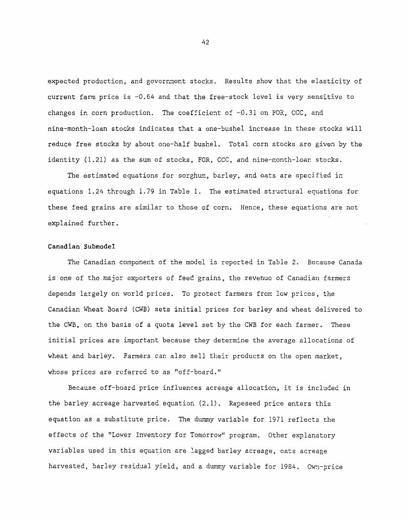
42
expected production, and government stocks. Results show that the elasticity of
current farm price is -0.64 and that the free-stock level is very sensitive to
changes in corn production. The coefficient of -0.31 on FOR, CCC, and
nine-month-loan stocks indicates that a one-bushel increase in these stocks will
reduce free stocks by about one-half bushel. Total corn stocks are given by the
identity (1.21) as the sum of stocks, FOR, CCC, and nine-month-loan stocks.
The estimated equations for sorghum, barley, and oats are specified in
equations 1. 24 through 1. 79 in Table 1. The estimated structural equations for
these feed grains are similar to those of corn. Hence, these equations are not
explained further.
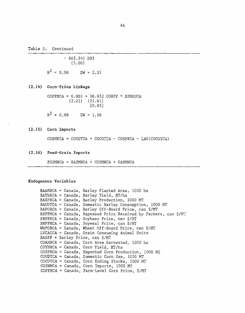
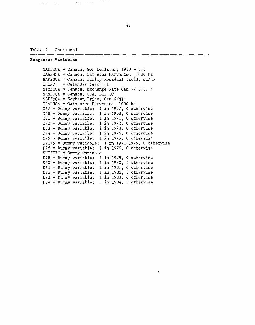
Canadian Submodel
The Canadian component of the model is reported in Table 2. Because Canada
is one of the major exporters of feed grains, the revenue of Canadian farmers
depends largely on world prices. To protect farmers from low prices, the
Canadian Wheat Board (CWB) sets initial prices for barley and wheat delivered to
the CWB, on the basis of a quota level set by the CWB for each farmer. These
initial prices are important because they determine the average allocations of
wheat and barley. Farmers can also sell their products on the open market,
whose prices are referred to as "off-board."
Because off-board price influences acreage allocation, it is included in
the barley acreage harvested equation (2.1). Rapeseed price enters this
equation as a substitute price. The dummy variable for 1971 reflects the
effects of the "Lower Inventory for Tomorrow" program. Other explanatory
variables used in this equation are lagged barley acreage, oats acreage
harvested, barley residual yield, and a dummy variable for 1984. Own-price

43
Table 2. Structural parameter estimates of the Canadian feed-grains submodel
(2.1) Barley Area Harvested
BAAHHCA = 2412.850 + 0.519 LAG(BAAHHCA) (3.87) (5.13)
+ 16.548 LAG(BAPOBCA/NARDDCA) (4.27)
- 3.811 LAG(RSPFMCA/NARDDCA) ( 3. 02)
[0.47] [-0.03]
- 0.592 (3. 71)
[-0.03]
OAAHHCA + 1286.530 D71 + 609.629 D84 (4.30) (1.85)
+ 1458.010 BARESCA (3.11)
DW = 1.98
(2.2) Barley Production
BASPRCA = BAAHHCA * BAYHHCA
(2.3) Barley Domestic Use
BAUDTCA = -48.141- 6.734 BAPOBCA/NARDDCA (0.04) (3.23)
[ -0. 12]
+ 2.759 ( 2. 72) [0.11]
SMPFMCA/NARDDCA + 382.406 LVCACCA (6.77) [ 1. 06]
- 1364.54(D67 + D68) - 765.259(D80 + D81 + D82 + D83 + D84) (6.39) (3.69)
DW = 2.13
(2.4) Barley Off-Board Price
BAPOBCA = 11.180 + 38.524 BARPF (2.17) (17.22)
[0.87]
DW = 1. 47
* NIMEUCA + 20.803 D73 (2.53)
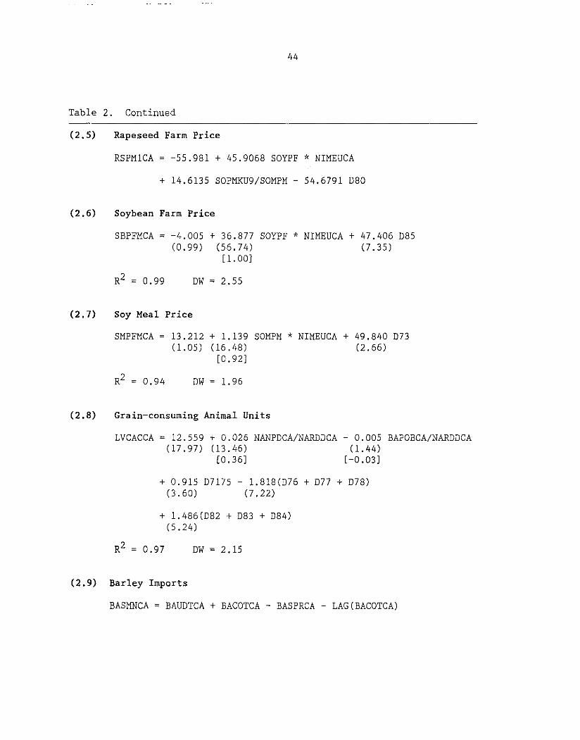
44
Table 2. Continued
(2.5) Rapeseed Farm Price
RSPM1CA -55.981 + 45.9068 SOYPF * NIMEUCA
+ 14.6135 SOPMKU9/SOMPM - 54.6791 080
(2.6) Soybean Farm Price
SBPFMCA = -4.005 + 36.877 SOYPF * NIMEUCA + 47.406 085 (0.99) (56. 74) (7.35)
[ 1. 00)
DW = 2.55
(2.7) Soy Meal Price
SMPFMCA = 13.212 + 1.139 SOMPM * NIMEUCA + 49.840 073 (1.05) (16.48) (2.66)
[0.92)
DW = 1.96
(2.8) Grain-consuming Animal Units
LVCACCA = 12.559 + 0.026 NANPDCA/NARDDCA (17.97) (13.46)
[0.36)
- 0.005 (1. 44)
[-0.03)
+ 0.915 07175 - 1.818(076 + D77 + D78) (3.60) (7.22)
+ 1.486(082 + 083 + 084) (5.24)
ow= 2.15
(2.9) Barley Imports
BAPOBCA/NARDDCA
BASMNCA = BAUDTCA + BACOTCA - BASPRCA - LAG(BACOTCA)
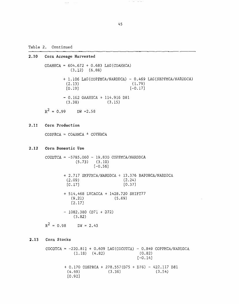
45
Table 2. Continued
2.10 Corn Acreage Harvested
COAHHCA = 604.672 + 0.683 LAG(COAHHCA) (3.12) (6.88)
+ 1.106 LAG(COPFMCA/NARDDCA) (2.13) [0.19)
- 0.162 OAAHHCA + 114.916 D81 (3.38) (3.15)
R2 = 0.99 DW =2.58
2.11 Corn Production
COSPRCA = COAHHCA * COYHHCA
2.12 Corn Domestic Use
- 0.469 LAG(SBPFMCA/NARDDCA) (1. 79)
[-0.17)
COUDTCA = -5785.060 - 19.830 COPFMCA/NARDDCA (5.73) (3.10)
[-0.56)
+ 2.717 SMPFMCA/NARDDCA + (2.09) [0.17)
13.376 BAPOBCA/NARDDCA (2.24) [0.37)
+ 514.468 LVCACCA + 1428.720 SHIFT77 (9.21) (5.69) [2.17)
- 1082.380 (D71 + D72) (3.82)
DW = 2.43
2.13 Corn Stocks
COCOTCA = -220.811 + 0.609 LAG(COCOTCA) - 0.849 COPFMCA/NARDDCA (1.18) (4.82) (0.82)
[-0.14)
+ 0.170 COSPRCA + 278.557(075 + D76) - 422.117 D81 (4.69) (3.36) (3.54) [0.92)
46
Table 2. Continued
- 663.341 D83 (5.00)
0. 98 DW = 2.35
(2.14) Corn-Price Linkage
COPFMCA = 6.801 (2. 21)
+ 36.932 (31. 61)
[0.93]
CORPF * NIMEUCA
R2 = 0,98 DW = 1.56
(2.15) Corn Imports
COSMNCA = COUDTCA + COCOTCA - COSPRCA - LAG(COCOTCA)
(2.16) Feed-Grain Imports
FGSMNCA = BASMNCA + COSMNCA + OASMNCA
Endogenous Variables
BAAHHCA BAYHHCA BASPRCA BAUDTCA BAPOBCA RSPFMCA SBPFMCA SMPFMCA WHPOBCA LVCACCA BARPF =
COAHHCA COYHHCA COSPRCA COUDTCA COCOTCA COSNMCA COPFMCA
Canada, Barley Planted Area, 1000 ha Canada, Barley Yield, MT/ha Canada, Barley Production, 1000 MT
= Canada, Domestic Barley Consumption, 1000 MT Canada, Barley Off-Board Price, can $/MT Canada, Rapeseed Price Received by Farmers, can $/MT Canada, Soybean Price, can $/MT Canada, Soymeal Price, can $/MT Canada, Wheat Off-Board Price, can $/MT Canada, Grain Consuming Animal Units
Barley Price, can $/MT Canada, Corn Area Harvested, 1000 ha Canada, Corn Yield, MT/ha
= Canada, Expected Corn Production, 1000 MT Canada, Domestic Corn Use, 1000 MT
= Canada, Corn Ending Stocks, 1000 MT Canada, Corn Imports, 1000 MT Canada, Farm-Level Corn Price, $/MT
47
Table 2. Continued
Exogenous Variables
NARDDCA Canada, GDP Deflater, 1980 = 1.0 OAAHHCA Canada, Oat Area Harvested, 1000 ha BARESCA Canada, Barley Residual Yield, MT/ha TREND = Calendar Year + 1 NIMEUCA = Canada, Exchange Rate Can $!U.S. $ NANPDCA Canada, GDA, BIL $C SBPFMCA Soybean Price, Can $/MT OAAHHCA Oats Area Harvested, 1000 ha D67 =Dummy variable: 1 in 1967, 0 otherwise D68 Dummy variable: 1 in 1968, 0 otherwise D71 = Dummy variable: 1 in 1971, 0 otherwise D72 Dummy variable: 1 in 1972, 0 otherwise D73 =Dummy variable: 1 in 1973, 0 otherwise D74 Dummy variable: 1 in 1974, 0 otherwise D75 Dummy variable: 1 in 1975, 0 otherwise D7175 =Dummy variable: 1 in 1971-1975, 0 otherwise D76 = Dummy variable: 1 in 1976, 0 otherwise SHIFT77 = Dummy variable D78 Dummy variable: 1 in D80 Dummy variable: 1 in D81 Dummy variable: 1 in D82 Dummy variable: 1 in D83 Dummy variable: 1 in D84 Dummy variable: 1 in
0 otherwise 0 otherwise
1978, 1980, 1981, 0 1982, 0 1983, 0 1984, 0
otherwise otherwise otherwise otherwise

48
elasticity of barley acreage harvested is 0.47 and cross-price elasticity is
-0.25. Barley production is given as acreage harvested times yield per acre.
On the demand side, only barley food use is endogenously estimated (2.3).
The variables that explain barley food use are off-board price, soybean-meal
price, grain-consuming animal units, and two shift variables for the late 1960s
and early 1980s. Own-price elasticity of barley food use is estimated at -0.12
and substitute-price elasticity is 0,11. Barley off-board price, rapeseed farm
price, soybean farm price, and soybean-meal price are endogenously estimated.
Grain-consuming animal units are endogenously estimated as a function of real
barley price, real income, and d~~y variables. Because barley is an input in
livestock production, barley price has a negative effect on the number of
grain-consuming animal units. Barley imports (2.9) are defined as total use
minus total supply.
The CWB does not exercise its policy over the corn market. Corn and barley
are produced in different regions of Canada. The soybean is the substitute crop
for corn in production. Therefore soybean price is included in corn acreage
(2.10). Oats acreage harvested is also included in corn acreage. The other
variables that enter the corn-acreage equation are corn price and a dummy
variable. Own-price elasticity is 0.19 and substitute-price elasticity, -0.17.
Corn yield is exogenous. Therefore, production is obtained by multiplying
acreage and yield.
On the demand side, domestic corn use and stock demand are endogenously
estimated. The variables that enter the domestic use equation are corn price,
soybean-meal and barley prices (as substitute prices), grain-consuming animal
units, and dummy variables. Own-price elasticity is -0.56, and cross-price

49
elasticities are 0.17 for soybean-meal price and 0.37 for barley price. Because
corn is an input in the livestock sector, the number of grain-consuming animal
units is included to reflect the demand for corn in the livestock production as
derived demand for corn.
Corn ending stocks are estimated as a function of corn price, production,
lag inventories, and dummy variables. The price elasticity of stock demand is
estimated at -0.14. Current crop production has a positive effect on stock
demand. The Canadian corn price at the farm level is linked to the U.S. farm
price (2.14). Corn imports (2.15) are defined as total use minus total supply.
Total feed-grain imports (2.16) are equal to barley imports, corn imports, and
oats imports.
Australian Submodel
The Australian component of the model is reported in Table 3. Australia
traditionally has exported barley, which is the major feed-grain crop produced
in this region. Wheat and barley are substitute crops both in terms of
production and consumption. The barley-acreage equation (3.1) is estimated as a
function of lagged barley prices and wheat prices, lagged acreage, wool price,
and two dummy variables for 1967 and 1973. These dummy variables make
allowances for changes in the Australian government's domestic policies
regarding barley production. Wool price is included in the acreage equation
because the land could be used for grazing sheep. Total production (3.2) is
given as acreage harvested times yield.
On the demand side, barley domestic use and stocks are modeled. Domestic
use (3.3) is estimated as a function of barley price (own price), wheat price
(substitute price), income, and two dummy variables. Own-price elasticity is

50
Table 3. Structural parameter estimates of the Australian feed-grains submodel
(3.1) Barley Area Harvested
BAAHHAU = 1181.580 + 0.551 LAG(BAAHHAU) (1.47) (3.94)
+ 0.116 LAG(BAPFMAU/NARDDAU) (2.68) [0. 60]
- 0.076 LAG(WHPFMAU/NARDDAU) (-1.80) [-0.46]
- l. 955 (-1.03) [-0.20]
LAG(GWPFMAU/NARDDAU) - 665.054 D67 (-2.15)
- 88.180 D73 + 610.208 (D83 + D84 + D85) (-0.20) (3.62)
R2 0.91 DW(1) = 1.41 DW(2) = 2.31
(3.2) Barley Production
BASPRAU = BAAHHAU * BAYHHAU
(3.3) Domestic Barley Uses
BAUDTAU = 1540.550- 0.128(BAPFMAU/NARDDAU) (4.40) (-6.19)
[-1.27]
+ 0.056(WHPFMAU/NARDDAU) ( 3. 43) [0. 66]
+ 3.752(NANPDAU/NARDDAU) (1. 99) [0. 38]
+ 335.239 D81 (2.81)
- 602.548(084 + D85 + D86)- 318.71 D69 (-5.74) (-2.48)
R2 0.87 DW(l) 1.57 DW(2) = 2.07

51
Table 3. Continued
(3.4) Barley Ending Stocks
BACOTAU = 794.707- 0.038(BAPFMAU/NARDDAU) (7.66) (-5.17)
[ -1. 85]
+ 0.189 LAG(BACOTAU) - 353.629 SHIFT79 (1.69) (-7.92) [0.19]
+ 119.724(D80 + D82) - 212.868(D72 + D77) (2.08) (-4.11)
R2 = 0.87 DW(l) = 2.32 DW(2) = 1.46
(3.5) Barley Prices
BAPFMAU = -283.784 + 556C.210(BARPF * NIMEUAU) (-0.51) (17 .57)
[ l. 05]
+ 3200.200 D82 - 3872.090(D84 + D85) (3.67) (-4.96)
R2 = 0.96 DW(l) 1.41 DW(2) = 1.39
(3.6) Sheep Inventory
SHCOTAU = 17.337 + 0.811 LAG(SHCOTAU) (1.04) (8.27)
- 0.001 LAG(SGPFMAU/NARDDAU) (-0.63) [-0.06]
+ 0.062 LAG(GWPFMAU/NARDDAU) (2.16) [0 .10]
+ 0.137 LAG[LAG(GWPFMAU/NARDDAU)] (2.75) [0.23]
- 0.002 LAG(WHFPMAU/NARDDAU) + 10.24(D84 + D85) (-1.63)
[-.21]
R2 0.91 DW(l) 2.15 DW(2) 1.48

52
Table 3. Continued
(3.7) Greasy-wool Farm Price
GWPFMAU = 83.910 + 318.458(COLFAU * NIMEUAU) (1.35) (8.10)
[0.75]
+ 1.020(LTARCRUD * NIMEUAU) - 0.409 LAG(SHCOTAU) (1.38) (-1.14) [0.08]
+ 91.326 D72 + 55.869 D86 + 55.256 D81 + 48.206 D73 (5.62) (2.89) (2.94)
R = 0.98 DW(1) = 1.99 DW(2) = 2.49
(3.8) Barley Net Imports
BASMNAU = BAUDTAU + BACOTAU - BASPRAU - LAG(BACOTAU)
(3.9) Sorghum Prices
SGPFMAU = -301.650 + 5099.8SO(SORPF * NIMEUAU) (-0.87) (24.54)
[ 1. 07]
- 2691.54(D83 + D84 + D85) + 1342 D86 (-6.07) (2.72)
R2 = .98 DW(1) = 2.03 DW(2) 2.75
(3.10) Sorghum Area Harvested
SGAHHAU = 277.240 + 0.809 LAG(SGAHHAU) + 0.025 LAG(SGPFMAU/NARDDAU) (3.40) (14.56) (3.24)
- 0.014 LAG(WHPFMAU/NARDDAU) ( 1. 97)
[-0.35]
[0.50]
- 0.018 LAG(BAPFMAU/NARDDAU) (2.86)
[-0.40]
+ 124.448 D80- 247.635 D73- 188.930 D77 (3.51) (5.68) (4.42)
DW(1) 1. 78 DW(2) 2. 32

53
Table 3. Continued
(3.11) Sorghum Production
SGSPRAU = SGAHHAU * SGYHHAU
(3.12) Sorghum Stock
SGCOTAU = 6.468 + 0.288 LAG(SGCOTAU) + 0.028 SGSPRAU (2.63) (1.68)
+ 93.584 072 + 108.016(076 + 077 + 079) (3.45) (6.02)
- 51.736 084 (1.87)
OW(l)
(3.13) Sorghum Imports
2.48 OW (2) 1.90
SGSMNAU = 977.377- 0.047(SGPFMAU/NARDOAU) (3.50) (2.40)
- 1.098 SGSPRAU- 176.122(073 + 074) (12.17) (1.63)
OW(1) = 1.78 OW(2) 2.12
(3.14) Market Equilibrium
SGUOTAU = SGSPRAU + LAG(SGCOTAU) + SGSMNAU - SGCOTAU
(3.15) Wheat Farm Price
WHPFMAU = - 135.300 + (0.40)
- 1604.540 077
100.531 WHPEXAU -(38.49)
[ 1. OS]
R2 0. 99 OW(l) = 2.31 OW(2)
3271.930(072 + 073) ( 8. 24)
1.29

54
Table 3. Continued
(3.16) Wheat Export Price
WHPEXAU = 4.059 + 0.973 WHPGPU90 * NIMEUAU + 23.400 D82 (0.67) (17.87) (2.38)
- 22.92(D84 + D85 + D86) ( 3. 09)
0.97 DW(l) 1. 35 DW(2)
(3.17) Feed-Grain Imports
FGSMNAU = BASMNAU + COSMNAU + OASMNAU
Endogenous Variables
= Barley Area Harvested, 1000 ha = Barley Ending Stocks, 1000 MT
2.55
BAAHHAU BACOT AU BAPFMAU BAUDTAU SGPFMAU SHCOTAU GWPFMAU BASMNAU BASPRAU SGAHHAU SGSPRAU SGCOTAU SGSMNAU SGUDTAU WHPFMAU WHPEXAU FGSMNAU
= Barley prices at farm level, AUS $/MT Domestic Barley Consumption, 1000 MT Sorghum prices at farm level, AUS $/MT
= Sheep inventories, mil head Greasy-wool producer price (cents/kg)
= Barley net imports, 1000 MT Barley production, 1000 MT
= Sorghum Area Harvested, 1000 ha Sorghum Production, 1000 MT Sorghum Stocks, 1000 MT
= Sorghum Imports, 1000 MT = Sorghum Use, 1000 MT
Wheat Farm Price, AUS $/MT Wheat Export Price, AUS $/MT Feed-Grain Imports, $1000 MT
Exogenous Variables
TREND = Time Trend NARDDAU Gross Domestic Product Deflator, 1980=1.0 BAYHHAU Barley Yield, MT/ha NIMEUAU = Exchange Rate ($US/$AUS) NANPDAU GDP, Bil $AV LTARCRUD = Grain-consuming Animals, 1000 heads D67 1 in 67, 0 otherwise D69 = 1 in 69, 0 otherwise D73 lin 73, 0 otherwise
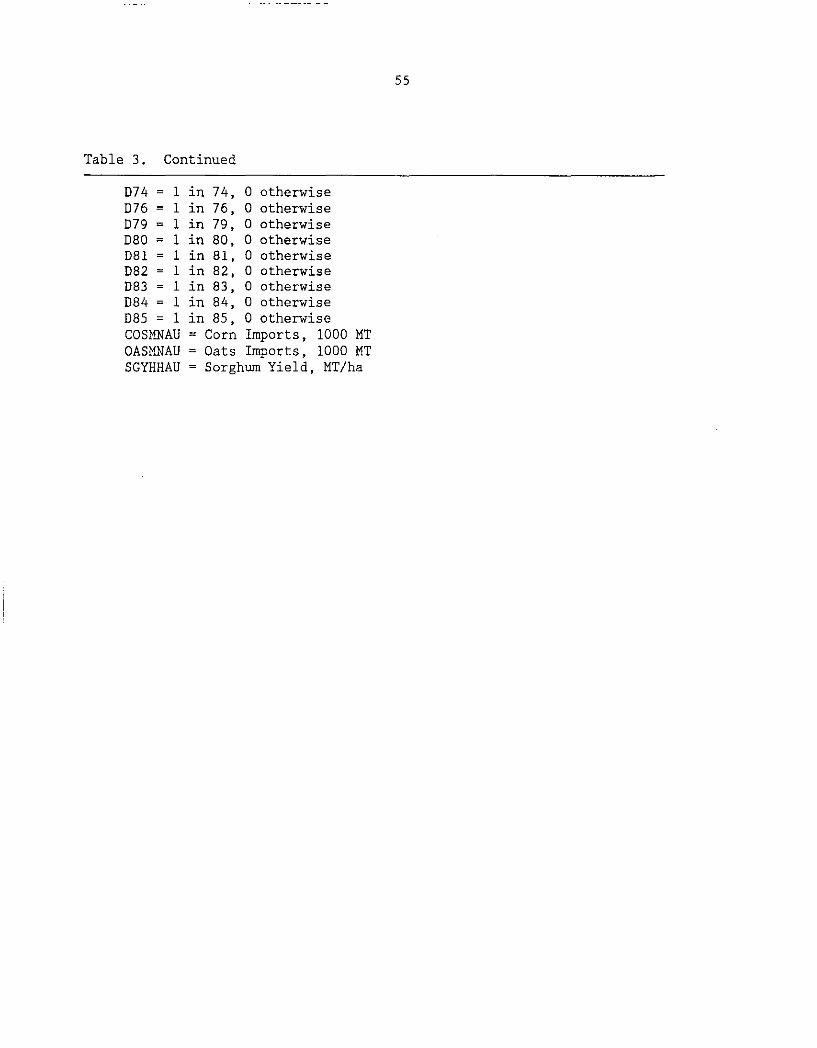
55
Table 3. Continued
074 1 in 74, 0 otherwise 076 1 in 76, 0 otherwise 079 1 in 79, 0 otherwise 080 = 1 in 80, 0 otherwise 081 1 in 81, 0 otherwise 082 1 in 82, 0 otherwise 083 1 in 83, 0 otherwise 084 1 in 84, 0 otherwise 085 1 in 85, 0 otherwise COSMNAU = Corn Imports, 1000 MT OASMNAU = Oats Imports, 1000 MT SGYHHAU Sorghum Yield, MT/ha

56
-1.27 and cross-price elasticity is 0.66. The explanatory variables in the
barley stock-demand equation (3.4) are lag stocks, barley price, and dummy
variables. The price-linkage relation is described by equation (3.5), in which
barley farm price is linked to the U.S. barley price. Because Australia does
not practice any trade restrictions in barley trade, price-transmission
elasticity is close to one. Sheep inventories (3.6) and greasy-wool (3.7) farm
prices are also endogenously estimated. Barley net imports are given by (3.8).
The supply side of the sorghum market is very similar to that of the
barley market; on the demand side, stocks and imports are endogenously
estimated, Feed-grains imports (3.17) are equal to barley, corn, and oats
imports.
Argentine Submodel
Argentina is a ~ompetitor of the United States in the feed-grains export
market. Argentina earns its foreign exchange through its agricultural exports
and has a good potential to increase production. Agricultural exports are also
a source of government revenue, through the export tax. The Argentine component
of the model is reported in Table 4,
Corn planted area (4.1) is influenced by both corn and soybean prices.
Other variables that enter the acreage equation are lagged acreage and two dummy
variables. The elasticity of area harvested with respect to corn price is 0.36
and with respect to soybean farm price is -0.21. Corn yield is exogenous in the
model. Corn production is given by the identity (4.2) as corn acreage times
yield.

57
Table 4. Structural parameter estimates of the Argentine feed-grains submodel
(4.1) Corn Area Harvested
COAHHAR = 1130.980 + 4.059 LAG(COPFMARR) (2.51) (3.65)
[. 36]
- 1.084 LAG(SBPFMARR) (-2.67)
+ 0.49 LAG(COAHHAR) (3.55)
[-0.21]
+ 553.482 D72 - 473.278(071 + D79) (2.32) (-2.58)
R2 = 0.83 DW(1) = 1.90
(4.2) Corn Production
COSPRAR = COAHHAR * COYHHAR
(4.3) Domestic Corn Use
COUDTAR = -915.573 - 3.647 COPFMARR (-0.51) (-1.37)
+ 6.473 (1.70) [0. 44]
[-0.31]
SGPFMARR + 0.184 COSPRAR (6.58) [0.45]
+ 47.910 CECOTAR + 650.868 D83 (1.84) (2.62) [0. 78]
+ 753.055 D71- 905.072 D70- 715.797 SHIFT75 (3.26) (-3.63) (-4.62)
R2 0.89 DW(l) 2.55
(4.4) Corn Ending Stocks
COCOTAR = 1137.360- 2.973 (6.26) (-6.43)
[-2.94]
COPFMARR + 0.017 (1.38) [0. 50]
COSPRAR

58
Table 4. Continued
- 367.522(078 + D79 + DBO) - 284.210 D83 (-5.57) (-2.85)
- 243.050(071 + 073) (-3.30)
R2 = 0.85 OW(1) = 2.76
(4.5) Corn Prices
COPFMARR = 154.329 + 21.800(CORPF * NIMECARF/WPI80AR * 10,000) (3.69) (4.08)
[0.62)
- 10.876[WPI80AR- LAG(WPI80AR))/LAG(WPI80AR) (-2.90) [-0.07)
- 233.557 074 - 33.510(073 + 075) (-5.93) (-3.06)
R2 = 0.76 DW(1) = 2.18
(4.6) Livestock Ending Inventories
CECOTAR = 26.777 + 0.0005 (4.04) (2.20)
[0.23)
NARPOAR - 0.024 (-2.82) [-0.10)
SGPFMARR
- 2.953 070 + 2.65(075 + 076 + 077) (-2.65) (3.22)
R2 = 0.96 OW(1) 1.57
(4.7) Corn Net Imports
COSMNAR = COUOTAR + COCOTAR - COSPRAR - LAG(COCOTAR)
(4.8) Sorghum Area Harvested
SGAHHAR = 993.659 + 0.474 LAG(SGAHHAR) + 5.615 LAG(SGPFMARR) (1.81) (3.84) (2.72)
[9.15)
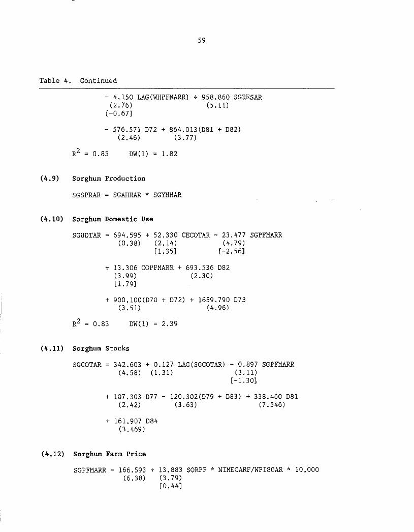
59
Table 4. Continued
- 4.150 LAG(WHPFMARR) + 958.860 SGRESAR (2.76) (5.11)
[ -0. 67]
- 576,571 D72 + 864.013(D81 + D82) (2.46) (3.77)
DW(l) 1.82
(4.9) Sorghum Production
SGSPRAR = SGAHHAR * SGYHHAR
(4.10) Sorghum Domestic Use
SGUDTAR = 694.595 (0.38)
+ 52.330 (2.14) [1.35]
CECOTAR - 23.477 (4.79)
[-2.56]
+ 13.306 COPFMARR + 693.536 D82 (3.99) (2.30) [ 1. 79]
+ 900.100(D70 + D72) + 1659.790 D73 (3.51) (4.96)
R2 = 0.83 DW(l) 2.39
(4.11) Sorghum Stocks
SGPFMARR
SGCOTAR = 342.603 + 0.127 LAG(SGCOTAR) - 0.897 SGPFMARR (4.58) (1.31) (3.11)
[-1.30]
+ 107,303 D77- 120.302(D79 + D83) + 338.460 D81 (2.42) (3.63) (7.546)
+ 161.907 D84 (3. 469)
(4.12) Sorghum Farm Price
SGPFMARR = 166.593 + 13.883 SORPF * NIMECARF/WPI80AR * 10,000 (6.38) (3.79)
[ 0. 44]

60
Table 4. Continued
R2 = 0.81
- 12.300[WPI80AR- LAG(WPI80AR)]/LAG(WPI80AR) (5.22)
[-0.09]
- 149.428 D74 - 18.063(073 + D75) (6.02) (1.09)
DW = 2.34
(4.13) Sorghum Imports
SGSMNAR = SGUDTAR + SGCOTAR - SGSPRAR - LAG(SGCOTAR)
(4.14) Soybean Farm Price
SBPFMARR = 194.490 + 25.374 SOYPF * NIMECARF/WPI80AR * 10,000
R2 = 0.89
(2.50) (6.67) [0. 80]
- 43.903[WPI80AR- LAG(WPI80AR)]/LAG(WPI80AR) (5.42)
- 222.841 D74 + 400.807 D75 + 134.495 D82 (3.25) (5.84) (2.05)
DW = 1.37
(4.15) Wheat Farm Price
WHPFMARR = 239.884 + 13.509(WHEPF NIMECARF/WPISOAR) * 10,000 (5.05) (2. 78)
R2 0.85
[ 0. 43]
- 17.143[WPI80AR- LAG(WPI80AR)]/LAG(WPI80AR) (4.93)
- 130.853(073 + D75) - 192.142 D74 + 7.8. 999 D77 ( 3. 65) (4.32) (2.65)
+ 85.845 D80 (2. 87)
DW( 1) = 2.06
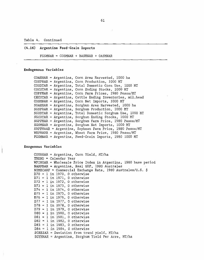
61
Table 4. Continued
(4.16) Argentine Feed-Grain Imports
FGSMNAR = COSMNAR + BASMNAR + OASMNAR
Endogenous Variables
COAHHAR Argentina, Corn Area Harvested, 1000 ha COSPRAR = Argentina, Corn Production, 1000 MT COUDTAR Argentina, Total Domestic Corn Use, 1000 MT COCOTAR Argentina, Corn Ending Stocks, 1000 MT COPFMAR Argentina, Corn Farm Prices, 1980 Pesos/MT CECOTAR = Argentina, Cattle Ending Inventories, mil.head COSMNAR Argentina, Corn Net Imports, 1000 MT SGAHHAR Argentina, Sorghum Area Harvested, 1000 ha SGSPRAR Argentina, Sorghum Production, 1000 MT SGUDTAR = Argentina, Total Domestic Sorghum Use, 1000 MT SGCOTAR Argentina, Sorghum Ending Stocks, 1000 MT SGPFMAR Argentina, Sorghum Farm Price, 1980 Pesos/MT SGSMNAR Argentina, Sorghum Net Imports, 1000 MT SBPFMAAR = Argentina, Soybean Farm Price, 1980 Pesos/MT WHFMARR Argentina, Wheat Farm Price, 1980 Pesos/MT FGSMNAR = Argentina, Feed-Grain Imports, 1980 1000 MT
Exogenous Variables
COYHHAR = Argentina, Corn Yield, MT/ha TREND = Calendar Year WPI80AR = Wholesale Price Index in Argentina, 1980 base period NARPDAR =Argentina, Real GDP, 1980 Australes NIMECARF = Commercial Exchange Rate, 1980 Australes/U.S. $ D70 l in 1970, 0 otherwise D7l l in 1971, 0 otherwise D72 l in 1972, 0 otherwise D73 = l in 1973, 0 otherwise D74 l in 1974, 0 otherwise D75 l in 1975, 0 otherwise D76 1 in 1976, 0 otherwise D77 1 in 1977, 0 otherwise D78 1 in 1978, 0 otherwise D79 = 1 in 1979, 0 otherwise D80 = l in 1980, 0 otherwise D8l = 1 in 1981, 0 otherwise D82 = l in 1982, 0 otherwise D83 = l in 1983, 0 otherwise D84 1 in 1984, 0 otherwise SGRESAR Deviation from trend yield, MT/ha SGYHHAR = Argentina, Sorghum Yield Per Acre, MT/ha

62
On the demand side, corn domestic use and ending stocks are endogenously
estimated. The explanatory variables in the corn domestic use equation (4.3)
are corn price, sorghum price, production, cattle stocks, and dummy variables.
Own-price elasticity of domestic corn use is -0.31. Sorghum is the major
substitute for corn in feed use. The substitute-price elasticity is 0.44.
Because corn is an input in the livestock sector, cattle stock is included in
the equation to reflect the demand for corn in livestock production--i.e.,
derived demand for corn.' Corn ending stocks (4.4) are modeled as a function of
corn farm price, corn production, and dummy variables. In equation 4.5, corn
farm prices are linked to U.S. farm prices. Total livestock ending stocks (4.6)
are endogenously estimated as a function of sorghum farm price, real income, and
dummy variables. Net corn imports are given by the identity (4.7).
The other major coarse grain produced in Argentina is sorghum. The
structure of the sorghum market is similar to that of the corn market.
Estimated equations for sorghum are given in equations 4.8 to 4.13. Soybean and
wheat price-linkage equations are given in equations 4.14 and 4.15. Argentina's
total feed-grain exports--the sum of corn, barley, and sorghum--are specified in
equation 4.16.
The European Community Submodel
The feed grains modeled for the EC are barley and corn, which the
community exports and imports, respectively. Before the estimated equations are
described, a summary of the EC's grain policies is provided.
Common Agricultural Policy (CAP) price-support policies regulate markets
via selected policy instruments to maintain grain prices to producers at
predetermined levels generally well above those of the world market. Market

63
supplies are controlled through government intervention, import restrictions,
and aggressive export policies. The policy prices in operation are the target
price, the threshold price, and the intervention price.
The target price is the price considered to be acceptable in the most
grain-deficient area (Duisburg, Germany). The intervention price is equal to
the target price minus transport costs from the largest grain surplus area
(Ormes, France) to Duisburg, plus a "market element" to the intervention price.
The intervention price is the price at which government agencies buy commodities
for storage and is thus a "supported price level." The threshold price
represents the lowest price at which imported grain can enter the EC without
depressing prices below the target-price level. The threshold price is equal to
the target price minus the transportation and marketing costs from Rotterdam to
Duisburg.
The variable levy for imports is equal to the threshold price minus the
world price. The variable levy paid by importers is a source of revenue for the
EC budget and for the European Agricultural Guarantee and Guidance Fund (EAGGF).
Export restitutions are export subsidies paid grain exporters to bridge the gap
between internal market price and world-market price and thus to make EC exports
competitive on the export market. These export payments are a drain on the
EAGGF. Further details concerning EC grain policies can be found in Burtin
(1987), Miller (1987), and OECD (1987).
The estimated equations are given in Table 5. Barley area harvested (5.1)
is estimated as a function of real barley intervention price, oats area
harvested, lag barley area harvested, and dummy variables. Because oats
competes with barley for acreage, oats acreage enters into the barley area
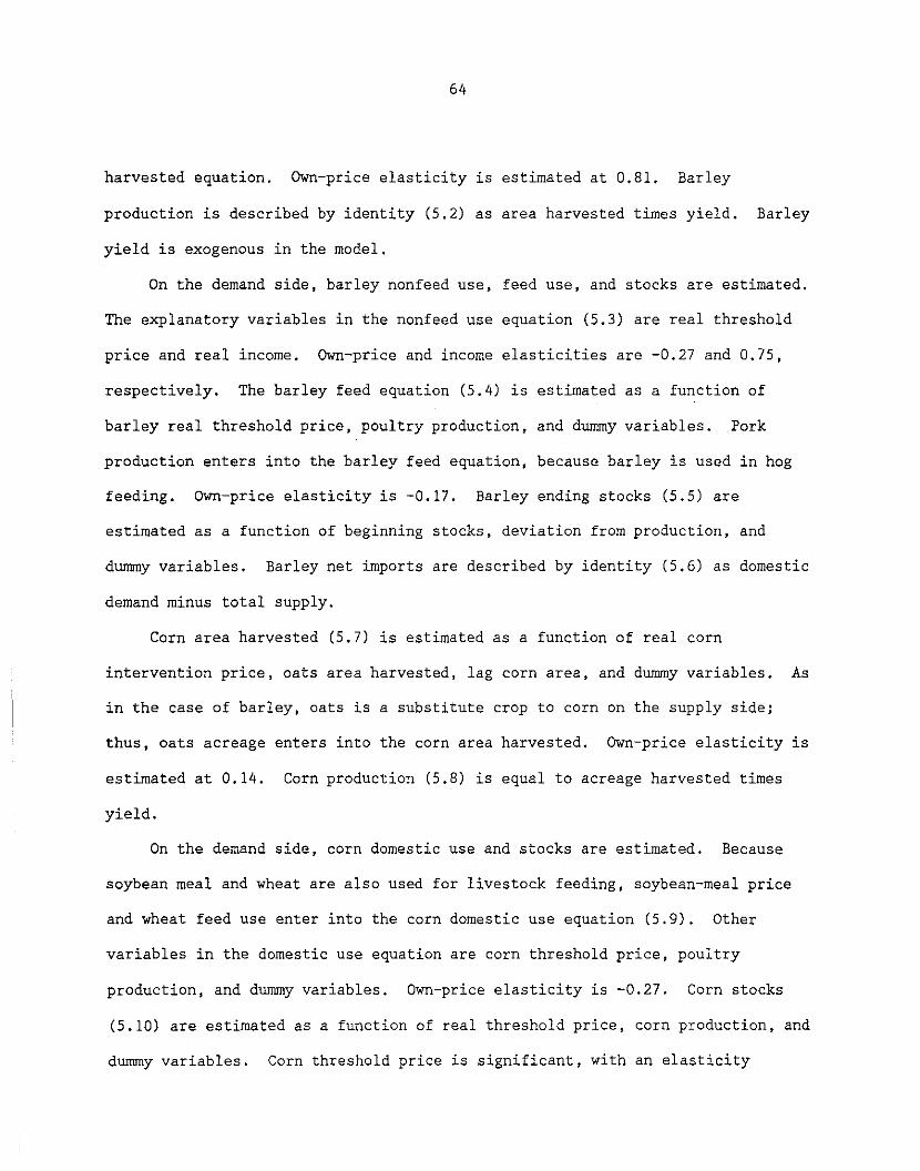
64
harvested equation. Own-price elasticity is estimated at 0.81. Barley
production is described by identity (5.2) as area harvested times yield. Barley
yield is exogenous in the model.
On the demand side, barley nonfeed use, feed use, and stocks are estimated.
The explanatory variables in the nonfeed use equation (5.3) are real threshold
price and real income. Own-price and income elasticities are -0.27 and 0.75,
respectively. The barley feed equation (5.4) is estimated as a function of
barley real threshold price, poultry production, and dummy variables. Pork
production enters into the barley feed equation, because barley is used in hog
feeding. Own-price elasticity is -0.17. Barley ending stocks (5.5) are
estimated as a function of beginning stocks, deviation from production, and
dummy variables. Barley net imports are described by identity (5.6) as domestic
demand minus total supply.
Corn area harvested (5.7) is estimated as a function of real corn
intervention price, oats area harvested, lag corn area, and dummy variables. As
in the case of barley, oats is a substitute crop to corn on the supply side;
thus, oats acreage enters into the corn area harvested. Own-price elasticity is
estimated at 0.14. Corn production (5.8) is equal to acreage harvested times
yield.
On the demand side, corn domestic use and stocks are estimated. Because
soybean meal and wheat are also used for livestock feeding, soybean-meal price
and wheat feed use enter into the corn domestic use equation (5.9). Other
variables in the domestic use equation are corn threshold price, poultry
production, and dummy variables. Own-price elasticity is -0.27. Corn stocks
(5.10) are estimated as a function of real threshold price, corn production, and
dummy variables. Corn threshold price is significant, with an elasticity

65
Table 5, Structural parameter estimates of the European Community feed-grains submodel
(5.1) Barley Acreage Harvested
BAAHHE2 = 5564.110 + 0.578 LAG(BAAHHE2) (4.88) (7.78)
+ 4.356 BAPIEO/NARDDEO - 0.578 OSAHHE2 + 523.498 D75 (3.16) (3.05) (4.02) [0.08]
+ 452.063 D7781 + 492.411 DEC9 (3.99)
R2 0. 99 DW = 2.39
(5.2) Barley Production
BASPRE2 = BAAHHE2 * BAYHHE2
(5.3) Barley Nonfeed Use
BAUHTE2 = 4683.180 - 9.620 BAPTHEO/NARDDEO (4.21) (6.84)
[-0.27]
+ 3.080 NANPDE2/NARDDEO + (8.57)
731.148(D74 + D75) ( 3. 45)
[0.75]
R2 0. 96 DW = 1. 83
(5.4) Barley Feed Use
BAUFEE2 = 22070.900 (2.69)
- 20.219 ( 1. 74)
[-0.17]
BAPTHEO/NARDDEO - 3701.070 SHIFT81 (6.38)
+ 1794.350(D77 + D78) - 1785.150(D74 + D75) (3.06) (3.05)
+ 1.641 POSPRE2 (2.80) [0. 48]
R2 0. 97 DW = 2.80

66
Table 5. Continued
(5.5) Barley Stocks
BACOTE2 = 2454.460 + 0.196 LAG(BACOTE2) + 1369.490 D82 (4.18) (1.06) (2.99)
- 1088.480(069 + D71 + D72 + D73) (4.16)
+ 2101.180 D84 + 1339.140 D85 (4.45) (2.30)
DW = 1. 62
(5.6) Barley Imports
+ 0.151 BARESE2 ( 3. 89) [0.02)
BASMNE2 = BAUFEE2 + BAUHcE2 + BACOTE2 - BASPRE2 - LAG(BACOTE2)
(5.7) Corn Acreage Harvested
COAHHE2 = 1381.610 + 0.827 LAG(COAHHE2) - 0.373 OSAHHE2 (3.35) (9.05) (2.89)
- 759.870 D76 - 288.497(080 + D81 + D83) (8.08) (4.78)
+ 2.440 COPIEO/NARDDEO (1.95) [0.14)
R2 = 0.94 DW = 1. 46
5.8 Corn Production
COSPRE2 = COAHHE2 * COYHHE2
5.9 Corn Domestic Use
COUDTE2 = 33770.200- 35.153 COPTHEO/NARDDEO (3.75) (2.03)
(-0.27)

67
Table 5. Continued
+ 11.1038 (3.94) [0. 09]
SMPFMEO/NARDDEO - 1.068 WHUFEE2 -(11.76) [-0.44]
- 3834.570(080 + D81 + D82) + 5.073 PYSPRE2 (4.54) (4.70)
R2 = 0.96 DW = 1.36
(5.10) Corn Stocks
COCOTE2 = 4945.430- 10.099 (3.09) (3.47)
[-0.77]
[ 0. 64]
COPTHEO/NARDDEO + 0,055 (1.14) [0. 30]
+ 2144.240 D74 - 1698.670(083 + D84) (5.99) (6.02)
+ 653.991(D76 + D77) (2.47)
DW = 1.87
(5.11) Corn Imports
COSMNE2 = COUDTE2 + COCOTE2 - COSPRE2 - LAG(COCOTE2)
(5.12) Pork Production
POSPRE2 = 5936.120 + 2.161 NANPDE2/NARDDEO (4.42) (6.18)
[0.54]
- 7.682 BAPTHEO/NARDDEO + 1168.570 SHIFT80 (3.26) (5.18)
- 0.465 SMPFMEO/NARDDEO (0. 71)
[-0.01]
R2 0. 98 DW = 1.61
[-0.21]
2400.280 D75 (1.77)
COSPRE2

68
Table 5. Continued
(5.13) Poultry Production
PYSPRE2 1375.180 + 1.655 NANPDE2/NARDDEO (2.40) (11.23)
- 4.465 (4.76)
[-0.27]
[0.90]
COPTHEO/NARDDEO + 654.949 SHIFT80 (6.73)
0.99 DW = 2.09
(5.14) Soy Meal Price
SMPFMEO = 15.910 + 1.130 SOMPM * NIMEUEO (2.72) (20.29)
[0.90]
0.98 DW = 2.59
(5.15) Feed-Grain Imports
FGSMNE2 = BASMNE2 + COSMNE2 + OASMNE2
Endogenous Variables
BAAHHE2 BACOTE2 BAUFEE2 BAUHTE2 BASPRE2 BASMNE2 COAHHE2 COCOTE2 COUDTE2 COSPRE2 COSMNE2 POSPRE2 PYSPRE2 SMPFME2 FGSMNE2
= EC Barley Area Harvested, 1000 ha = EC Barley Ending Stocks, 1000 MT = EC Barley Feed Use, 1000 MT
EC Barley Food Use, 1000 MT EC Barley Production, 1000 MT EC Barley Imports, 1000 MT
= EC Corn Area Harvested, 1000 ha = EC Corn Ending Stocks, 1000 MT = EC Corn Domestic Use, 1000 MT = EC Corn Production, 1000 MT
EC Corn Imports, 1000 MT = EC Pork Production, 1000 MT
EC Poultry Production, 1000 MT EC Soymeal Price, ECU/MT EC Feed-Grain Imports, 1000 MT
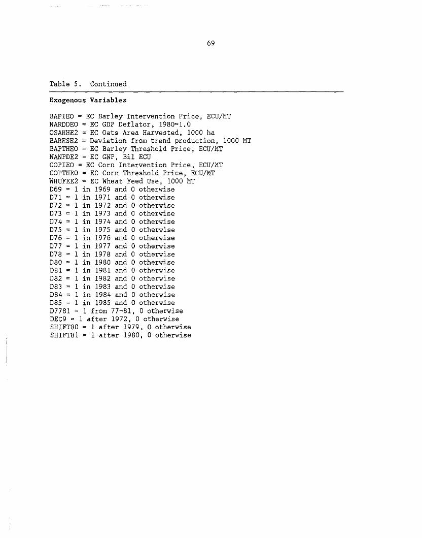
69
Table 5. Continued
Exogenous Variables
BAPIEO = EC Barley Intervention Price, ECU/MT NARDDEO = EC GDP Deflator, 1980=1.0 OSAHHE2 = EC Oats Area Harvested, 1000 ha BARESE2 Deviation from trend production, 1000 MT BAPTHEO EC Barley Threshold Price, ECU/MT NANPDE2 EC GNP, Bil ECU COPIEO = EC Corn Intervention Price, ECU/MT COPTHEO = EC Corn Threshold Price, ECU/MT WHUFEE2 = EC Wheat Feed Use, 1000 MT D69 1 in 1969 and 0 otherwise D71 = 1 in 1971 and 0 otherwise D72 = 1 in 1972 and 0 otherwise D73 = 1 in 1973 and 0 otherwise D74 1 in 1974 and 0 otherwise D75 = 1 in 1975 and 0 otherwise D76 1 in 1976 and 0 otherwise D77 1 in 1977 and 0 otherwise D78 = 1 in 1978 and 0 otherwise D80 = 1 in 1980 and 0 otherwise D81 = 1 in 1981 and 0 otherwise D82 1 in 1982 and 0 otherwise D83 = 1 in 1983 and 0 otherwise D84 = 1 in 1984 and 0 otherwise D85 1 in 1985 and 0 otherwise D7781 = 1 from 77-81, 0 otherwise DEC9 = 1 after 1972, 0 otherwise SHIFT80 1 after 1979, 0 otherwise SHIFT81 = 1 after 1980, 0 otherwise

70
estimate of -0.77. Corn imports (5.11) are equal to total domestic demand minus
domestic supply.
Poultry (5.12) and pork (5.13) production are also endogenized in the
model because these variables are used as explanatory variables in the
feed-demand equations. Economic Community soybean-meal price (5.14) is linked
to the U.S. soybean-meal price. Elasticity in the price-linkage equation is
0.90. The EC feed-grain imports are described by identity (5.15) as a sum of
the imports of barley, corn, and oats.
Thai Submodel
Because corn is the major feed grain produced and used in Thailand, only
this grain is modeled for the country. The Thai component of the model is
reported in Table 6. Corn area harvested (6.1) is estimated as a function of
real corn farm price, real sorghum farm price, time trend, and dummy variables.
Sorghum is a competing crop and thus its price enters the corn area-harvested
equation. Own-price elasticity is 0.16 and cross-price elasticity -0.14. Corn
production (6.2) is equal to corn area harvested times yield.
On the demand side, feed use and stock use are estimated. The explanatory
variables in the corn feed-use equation (6.3) are real corn farm price, corn
production, poultry production, and dummy variables. Own-price elasticity is
-0.12. Corn ending stocks (6.4) are estimated as a function of beginning
stocks, real corn farm price, and dummy variables. Own-price elasticity in
stock demand is -1.45. Corn imports are described by (6.5) as domestic demand
minus domestic supply.
Poultry production (6.6) is endogenously estimated as a function of real
corn farm price and real income. Input-price elasticity in this equation is

71
Table 6. Structural parameter estimates of the Thai feed-grains submodel
(6.1) Corn Area Harvested
COAHHTH = -1286998 (26.27)
+ 0.094 LAG(COPFMTH/NARDDTH) ( 1. 58) [0.16]
- 0.086 (0.75)
[-0.14]
LAG(SGPFMTH/NARDDTH) - 164.472 D778 (3.93)
- 67.928(076 + D77) + 169762 LOG(TREND) + 141.930 D71 (1. 78) (22.26) (2.84)
R2 0. 99
+ 84.120 D74 ( 1. 66)
DW = 2.07
(6.2) Corn Production
COSPRTH = COAHHTH * COYHHTH
(6.3) Corn Feed Use
COUFETH = -160.041 ( l. 17)
- 0.027 (0.44)
[-0.12]
COPFMTH/NARDDTH + 3.350 PLSPRTH (6.38)
+ 0.110 COSPRTH- 139.223 D7073 (2.20) (2.82) [0.61]
+ 222.858 DBO - 116.460 D81 (2.85) (1.28)
R2 0. 98 DW = 2.14
(6.4) Corn Stocks
COCOTTH = 268.164 + 0.117 LAG(COCOTTH) (3.24) (0.69)
[0.92]
- 0.082 COPFMTH/NARDDTH + 123.953 D70 (2.49) (2.44)
[-1.45]

72
Table 6. Continued
+ 129.343(075 + D82) - 101.245 D73 (2.05)
R2 0. 75 DW = 1.39
(6,5) Corn Imports
COSMNTH = COUFETH + COUHTTH + COCOTTH - COSPRTH - LAG(COCOTTH)
(6,6) Poultry Production
PLSPRTH = 45.019- 0.036 COPFMTH/NARDDTH (1.40) (3.00)
[-0.61]
+ 0.483 (16.61)
[ 2. 09]
NANPDTH/NARDDTH - 60.914 D7679 (5.21)
R2 0. 96 DW = 2.17
(6.7) Corn Price-Linkage Equation
COPFMTH = 24.950 + 34.758 (0.18) (11.97) [ l. 00]
R2 0.91 OW = 1.18
(6.8) Sorghum Price Linkage
CORPF * NIMEUTH - 592.534 073 (2.93)
SGPFMTH = 127.000 + 0.833 COPFMTH- 222.369 D74 (2.91) (27 .75) (3.38)
[0.86]
+ 683.487(081 + D82) (13.47)
R2 0. 99 DW = 1.18
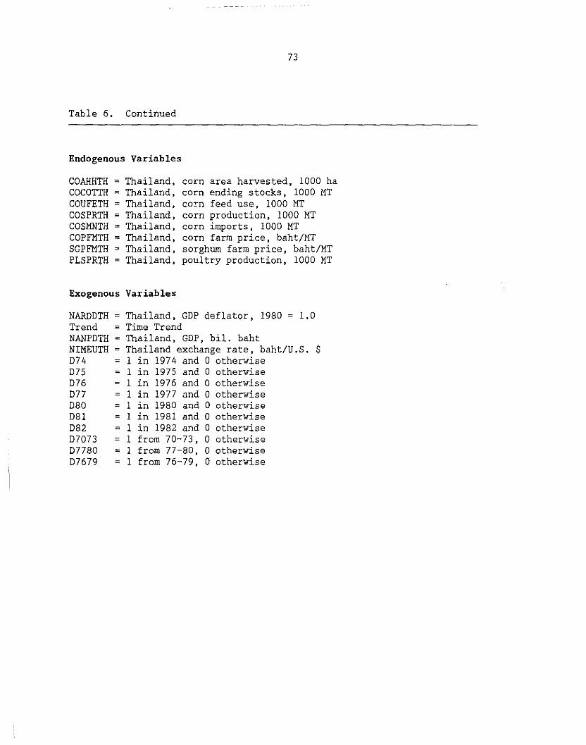
73
Table 6. Continued
Endogenous Variables
COAHHTH COCOTTH COUFETH COSPRTH COSMNTH COPFMTH SGPFMTH PLSPRTH
~ Thailand, ~ Thailand, ~ Thailand,
Thailand, Thailand,
~ Thailand, Thailand, Thailand,
corn area harvested, 1000 ha corn ending stocks, 1000 MT corn feed use, 1000 MT corn production, 1000 MT corn imports, 1000 MT corn farm price, baht/MT sorghum farm price, baht/MT poultry production, 1000 MT
Exogenous Variables
NARDDTH Trend NANPDTH NIMEUTH D74 D75 D76 D77 D80 D81 D82 D7073 D7780 D7679
Thailand, GDP deflator, 1980 1.0 ~ Time Trend
Thailand, GDP, bil. baht Thailand exchange rate, baht/U.S. $
~ 1 in 1974 and 0 otherwise ~ 1 in 1975 and 0 otherwise
1 in 1976 and 0 otherwise 1 in 1977 and 0 otherwise
~ 1 in 1980 and 0 otherwise 1 in 1981 and 0 otherwise 1 in 1982 and 0 otherwise 1 from 70-73, 0 otherwise
~ 1 from 77-80, 0 otherwise 1 from 76-79, 0 otherwise

74
-0.61. Corn price (6.7) in Thailand is linked to the U.S. corn price with a
price-transmission elasticity of 1.00. Sorghum price (6.8) is linked to the
Thai corn farm price.
South African Submodel
Two major feed grains produced and consumed in South Africa are corn and
sorghum. The estimated equations are presented in Table 7. Corn area harvested
(7.1) is estimated as a function of real corn farm price, lag area harvested,
and dummy variables. Supply-price elasticity is 0.04. Corn yield is exogenous
in the model. Corn use (7.2) is estimated as a function of real income and
dummy variables. The income coefficient is positive and significant. Income
elasticity is estimated at 0.28, Corn stocks (7.4) are endogenized in the
model. The explanatory variables in the stock equation are real corn farm
price, corn production (7.3), and dummy variables. Real corn farm price, with
an elasticity of -0.58, has a negative effect on stocks. Corn production has a
strong positive effect on stocks. Corn farm price (7.5) is linked to U.S. corn
farm price. Price-transmission elasticity is 1.26. The equilibrium identity is
given in equation (7.6).
Sorghum area harvested (7.7) is a function of real sorghum farm price,
wheat farm price, and dummy variables. Because wheat is a competing crop, wheat
price is used in the sorghum area harvested. Own-price elasticity is 0,95 and
cross-price elasticity is -0.82. Sorghum production (7.8) is described as
acreage times yield. Sorghum use (7.9) is estimated as a function of real
sorghum price and income. Demand-price elasticity is -0.30 and income
elasticity is 0.26. Sorghum stocks (7.10) are estimated as a function of real
sorghum price and production. Stock-price elasticity is -0.48, Sorghum

75
Table 7. Structural parameter estimates of the South African feed-grains submodel
(7.1) Corn Area Harvested
COAHHZA = 2031.360 + 0.512 LAG(COAHHZA) - 988.149 072 (3.63) (3.81) (11.53)
+ 456.140 073 - 266.049 SHIFT78 - 193.934(068 + 069) (3.51) (4.98) (2.51)
+ 0.883 LAG(COPFMZA/NARDOZA) * LAG(COYHHZA) (2.45) [0. 04)
OW= 1.36
(7.2) Corn Use
COUOTZA = 6046.490 + 33.690 NANPOZA/NARDOZA (7.81) (3.59)
[0.28)
+ 942.812 SHIFT73 + 676.624(081 + D82) (5.72) (4.29)
- 17.979 COPFMZA/NARDOZA (3.11)
[-0.36)
R2 = 0 96 . DW = 1.17
(7.3) Corn Production
COSPRZA = COAHHZA * COYHHZA
(7.4) Corn Stocks
COCOTZA = 12.903 + 0.265 (0.02) (13.89)
COSPRZA - 6.495 ( 1. 06)
[-0.58)
+ 302.226 D68 + 1382.990 D80 (1.64) (6.02)
OW= 1.36
COPFMZA/NARDOZA

76
Table 7. Continued
(7.5) Corn Farm Price
COPFMZA = -15.642 + 59.187 CORPF * NIMEUZA (2.79) (20.77)
[ l. 26]
- 33.210 D84- 37.339(D73 + D74 + D75) (2.63) (6.06)
DW = 2.15
(7.6) Corn Imports
COSMNZA = COUDTZA + COCOTZA - COSPRZA - LAG(COCOTZA)
(7.7) Sorghum Area Harvested
SGAHHZA = 217.154 (3.75)
+ 0.020 (9.75) [0.95]
LAG(SGPFMZA/NARDDZA)
+ 95.774 D71 + 126.415 D73- 0.011 LAG(WHPFMZA/NARDDZA) (4.38) (5.50) (3.60)
[-0.82]
- 77.117 D78 + 50.125 D69 (3.40) (2.15)
R2 = 0 93 . DW = l. 79
(7.8) Sorghum Production
SGSPRZA = SGAHHZA * SGYHHZA
(7.9) Sorghum Use
SGUDTZA = 16.646 - 0.008 SGPFMZA/NARDDZA (0.15) (2.32)
[-0.30]
+ 5.400 NANPDZA/NARDDZA + 0.193 SGSPRZA (3.50) (3.04) [0.95] [0.26]

Table 7. Continued
+ 133.729 D80 (2.92)
DW = 1. 86
(7.10) Sorghum Stocks
77
SGCOTZA = 16.706 + 0.316 SGSPRZA- 86,100(070 + D71) (0.49) (8.06) (4.27)
[ 1. 51]
- 151,896 083 - 0.004 SGPFMZA/NARDDZA (3.85) (1.50)
[ -0. 48]
DW = 2.51
(7.11) Sorghum Farm Price
SGPFMZA = 1050.390 + 0.933 SGPFMU9 * NIMEUZA (2.28) (12.70)
[0.83]
- 2471.500 D74 + 3982.420 082 + 1782.540 D69 (4.09) (5.65) (2.83)
- 1693.660 D72 (2.79)
DW = 2.04
(7.12) Sorghum Imports
SGSMNZA = SGUDTZA + SGCOTZA - SGSPRZA - LAG(SGCOTZA)
(7.13) Wheat Farm Price
WHPFMZA = 1827.880 + 4729.080 WHEPF * NIMEUZA (2.74) (12.90)
[0.85]

78
Table 7. Continued
+ 5446.900(D80 + D81 + D82) - 5752.210(D73 + D74 + D75) (5.90) (7.60)
0.98 DW = 2.34
(7.14) Feed-Grain Imports
FGSMNZA = COSMNZA + BASMNZA + OASMNZA
Endogenous Variables
COAHHZ = South Africa, Corn Area Harvested, 1000 ha COSPRZA = South Africa, Corn Production, 1000 MT COCOTZA = South Africa, Corn Stocks, 1000 MT COUDTZA South Africa, Corn Domestic Use, 1000 MT COPFMZA = South Africa, Corn Farm Price, Rand/MT COSMNZA = South Africa, Corn Imports, 1000 MT SGAHHZA Soth Africa, Sorghum Area Harvested, 1000 ha SGSPRZA South Africa, Sorghum Production, 1000 MT SGUDTZA South Africa, Sorghum Use, 1000 MT SGCOTZA = South Africa, Sorghum Stocks, 1000 MT SGPFMZA South Africa, Sorghum Farm Price, Rand/MT SGSMNZA South Africa, Sorghum Imports, 1000 MT WHPFMZA = South Africa, Wheat Farm Price, Rand/MT FGSMNZA = South Africa, Feed-Grain Imports, 1000 MT
Exogenous Variables
COYHHZA South Africa Corn Yield, MT/ha NARDDZA South Africa, GDP Deflator, 1980 1.0 NANPDZA South Africa, GDP Bil Rand NIMEUZA U.S. Exchange Rate, Rand/U.S.$ D68 1 in 1968 and 0 Otherwise D69 1 in 1969 and 0 Otherwise D70 1 in 1970 and 0 Otherwise D71 1 in 1971 and 0 Otherwise D72 1 in 1972 and 0 Otherwise D73 = 1 in 1973 and 0 Otherwise D74 = 1 in 1974 and 0 Otherwise D75 = 1 in 1975 and 0 Otherwise D78 1 in 1978 and 0 Otherwise D80 = 1 in 1980 and 0 Otherwise D81 1 in 1981 and 0 Otherwise D82 = 1 in 1982 and 0 Otherwise D83 1 in 1983 and 0 Otherwise D84 = 1 in 1984 and 0 Otherwise SHIFT73 One after 1972, 0 otherwise SHIFT78 = One after 1977' 0 otherwise

79
production is significant, with a positive effect on stocks. Sorghum farm price
(7.11) is linked to U.S. farm price, with a price transmission elasticity of
0.83. Sorghum imports (7.12) are described as domestic demand minus domestic
supply. Wheat farm price (7.13) is linked to U.S. wheat farm price.
Price-transmission elasticity is 0.85. Feed-grain imports (7.14) are defined as
the sum of imports of corn, barley, and sorghum imports.
Soviet Submodel
Until 1970 the Soviet Union was a significant net exporter of feed grains.
Since then, because of unstable weather and the economic policies, the Soviet
Union has become a major net importer of feed grains. The major feed grains
grown traditionally in the Soviet Union are oats and barley; in the past two
decades, however, corn has been introduced into Soviet agriculture. The grain
embargo of 1980 significantly changed Soviet policies toward grain imports.
Those changes included changes in the cropping pattern; i.e., deemphasizing
crops abundant in the world market, such as wheat, and emphasizing less abundant
crops such as corn.
The estimated equations are presented in Table 8. On the supply side,
feed-grain production is endogenously estimated. The independent variables used
in production (8.1) are feed-grain acreage harvested, feed-grain domestic use,
and a shift variable for the period 1970 and 1971. Acreage harvested is
described by identity (8.2) as production divided by yield.
Feed grains are used largely for feed, and their use is constrained by
production. Feed-grain domestic use (8.3) is estimated as a function of U.S.
corn price deflated by light Arabian crude-oil price, current production, and

80
livestock inventories. The United States corn price is used because a
consistent price series is unavailable, Own-price elasticity is estimated at
-0.07. Both livestock inventories and production have positive effects on the
domestic use of feed grains. Feed-grain ending stocks (8.4) are endogenously
estimated as a function of lag inventories, production deviation from its trend,
and dummy variables for 1977 and 1984. Livestock inventories (8.5) are
estimated as a function of income and lag livestock inventories. Equation (8.6)
equates the net import demand Qf feed grain to domestic demand minus
supply.
Chinese Submodel
As in the Soviet submodel, in the Chinese submodel total feed grains are
modeled (see Table 9). On the supply side, area is endogenously estimated. The
explanatory variables used in the feed-grain area harvested equation (9.1) are
feed-grain yield, lagged acreage, and dummy variables. Total production (9.2)
is given by the identity acreage times yield. Feed-grain use in China is
constrained by production. Thus, feed-grain domestic use (9.3) is estimated as
a function of production, hog inventories, and a shift variable for the period
1978-83. Income and lag hog inventories enter the hog inventories equation
(9.4) as explanatory variables. Feed-grain net imports are described by
identity (9.5) as domestic use minus production.
Eastern European Submodel
Production is endogenously estimated in the Eastern European submodel, as
in the Soviet submodel (see Table 10). The variables explaining feed-grain
production (10.1) in Eastern Europe are yield, lagged domestic use, and two
dummy variables for 1975 and 1979.

81
Table 8. Structural parameter estimates of the Soviet feed-grains submodel
(8.1) Feed-Grain Production
FGSPRSU = -43847.900 + 50542.900 FGYHHSU (-4.96) (10.59)
+ 0.446 LAG(FGUDTSU) - 11050.200(D70 + D71) (7.62) (-3.16)
R2 0.93 DW(1) = 1.57 DW(2) = 2.04
(8.2) Feed-Grain Area Harvested
FGAHHSU = FGSPRSU/FGYHHSU
(8.3) Feed-Grain Domestic Uses
FGUDTSU = -26713- 16961.100(CORPF/LTARCRUD) (-0.87) (-2.27)
[-0.07]
+ 613.463 CECOTSU + 0.635 FGSPRSU (2.47) (10.12)
- 7345.85(D82 + D83) (-3.15)
R2 = 0.98 DW(1) = 2.32 DW(2) = 1.99
(8.4) Feed-Grain Ending Stocks
FGCOTSU = 962.328 + 0.071 FGPRESSU (1.69) (5.17)
+ 0.787 LAG(FGOTSU) - 4242.930 D77 (5.71) (-5.11)
+ 2118.360 D84 (2.78)
R2 0.83 DW(l) = 1.55 DW(2) = 1.97

82
Table 8. Continued
(8.5) Animal Inventories
(8.6)
CECOTSU = 34.586 (5.42)
+ 0.023 (5.52) [ 0. 26]
0.99 DW(l) = 1. 89
Feed-Grain Net Imports
NANPGSU + 0.430 LAG(CECOTSU) (4.14)
DW(2) 2.53
FGSMNSU = FGUDTSU + FGCOTSU - FGSPRSU - LAG(FGCOTSU)
Endogenous Variables
FGAHHSU Soviet Union, total feed-grain area harvested, 1000 ha FGYHHSU = Soviet Union, feed-grain average yield, MT/hg FGSPRSU Soviet Union, feed-grain production, 1000 MT FDUDTSU = Soviet Union, feed-grain domestic use, 1000 MT FGCOTSU = Soviet Union, feed-grain ending stocks, 1000 MT CECOTSU Soviet Union, ending cattle inventories, mil head FGSMNSU Soviet Union, net imports of feed grains, 1000 MT
Exogenous Variables
TREND = Time Trend LTARCRUD =Light Arabian crude oil price (U.S. $/bbl.) NANPGSU = Soviet Union, real GDP, 1995 SUS FGPRESSU = Deviation of actual production from trend production D70 = 1 in 1970 and 0 Otherwise D71 = 1 in 1971 and 0 Otherwise D77 = 1 in 1977 and 0 Otherwise D82 1 in 1982 and 0 Otherwise D83 1 in 1983 and 0 Otherwise

83
Table 9. Structural parameter estimates of the Chinese feed-grains submodel
(9.1) Feed-Grain Area Harvested
FGAHHCN = 13512.500 + 873.488 FGYHHCN (5.03) (2.44)
+ 0.264 LAG(FGAHHCN) + 2477.420 D75 (1.67) (4.58)
+ 3423.170(076 + D77 + D78 + D79 + D80) (5.35)
- 1172.690 D85 + 1832.590 D81 (-2.14) (2.33)
R2 = 0.97 DW(1) = 1.49 DW(2) = 1.61
(9.2) Feed-Grain Production
FGSPRCN = FGAHHCN * FGYHHCN
(9.3) Feed-Grain Domestic Uses
FGUDTCN = 1943.290 + 0.854 FGSPRCN (1.56) (37.65)
+ 16.716 HOCOTCN + 4800.920 D7883 (2.34) (8.72)
R2 = 0. 998 DW(l) 1.58 DW(2) = 2.13
(9.4) Hog Inventories
HOCOTCN = 107.554 + 0.086 NANYNCN (4.84) (3.07)
+ 0.352 LAG(HOCOTCN) + 50.817 SHIFT71 (2.64) (4.33)
+ 25.160 D79 (2.21)
R2 0.96 DW(1) 1. 76 DW(2) 2.26

84
Table 9. Continued
(9.5) Feed-Grain Net Imports
FGSMNCN = FGUDTCN - FGSPRCN
Endogenous Variables
FRAHHCN FGYHHCN FGSPRCN FGUDTCN HOCOTCN FGSMNCN
= China, China, China, China,
= China, = China,
feed-grain area harvested, 1000 MT feed-grain average yield, MT/ha feed-grain production, 1000 MT feed-grain domestic use, 1000 MT hog ending inventories, mil head net imports of feed grains, 1000 MT
Exogenous variables
NANYNCN = China, net material product produced, bil D75 = 1 in 1975 and 0 Otherwise D76 1 in 1976 and 0 Otherwise D77 1 in 1977 and 0 Otherwise D78 1 in 1978 and 0 Otherwise D79 1 in 1979 and 0 Otherwise D80 1 in 1980 and 0 Otherwise D7883 1 from 78-83, 0 Otherwise SHIFT71 = 1 after 1970, 0 Otherwise
1980 yuan

85
Table 10. Structural parameter estimates of the Eastern European feed-grains submodel
(10.1) Feed-Grain Production
(10. 2)
(10.3)
(10.4)
FGSPRE8 = 2638.060 + 10085.100 FGYHHE8 ( 1. 72) (10. 86)
+ 0.211 LAG(FGUDTE8) + 3315.710 D75 (3.67) (2.92)
+ 2713.390 D79 (2.30)
R2 0.98 DW(1) ~ 2.16 DW(2) 2.47
Feed-Grain Uses
FGUDTE8 = -6599.810 + 0.741 FGSPRE8 (-2.21) (4.49)
+ 386.514 HOCOTE8 - 5549.630 SHIFT81 (3. 95) ( -4. 73)
+ 2709.450 D85 ( 1. 56)
R2 0.98 DW(1) = 1.46 DW(2) = 1.35
Feed-Grain Ending Stocks
FGCCOTE8 = -2150.610 + 0.092 FGSPRE8 (-5.84) (9.06)
+ 0.097 LAG(FGCOTE8) + 763.352 D69 (1.15) (3.45)
- 687.101(D72 + D73 + D74) + 717.713(D84 + D85) (-4.94) (4.11)
R2 0.97 DW(1) 2.02 DW(2)
Hog Inventories
HOCOTE8 = 1.082 + 16.519 NARPDIE8 (0.52) (2.25)
[0.24]
2.84

86
Table 10. Continued
+ 0.413 LAG(HOCOTE8) + 0.0004 LAG(FGUDTE8) (2.67) (2.62)
+ 5.762 D75 + 4.096 D77 - 4.281 D85 (3.55) (2.49) (-2.09)
0.99 DW(l) 1.80 DW(2) = 2.64
(10.5) Feed-Grain Net Imports
FGSMNE8 = FGUDTE8 + FGCOTE8 - FGSPRE8 - LAG(FGCOTE8)
Endogenous Variables
FGYHHE8 = Eastern Europe, Expected Average Yields, MT/ha FGSPRE8 = Eastern Europe, Expected Feed-Grain Production, 1000 MT FGUDTE8 = Eastern Europe, Domestic Total Feed-Grain Uses, 1000 MT FGCOTE8 Eastern Europe, Ending Feed-Grain Stocks, 1000 MT HOCOTE8 Eastern Europe, Ending Hog Inventories, mil head FGSMNE8 Eastern Europe, Net Imports of Feed Grains, 1000 MT
Exogenous Variables
NARPDIE8 = Eastern Europe; Real GDP Index; 1980 1.0 D69 1 in 1969 and 0 Otherwise D72 1 in 1972 and 0 Otherwise D73 = 1 in 1973 and 0 Otherwise D74 1 in 1974 and 0 Otherwise D75 = 1 in 1975 and 0 Otherwise D79 1 in 1979 and 0 Otherwise D84 = 1 in 1984 and 0 Otherwise D85 = 1 in 1985 and 0 Otherwise SHIFT81 = 1 after 1980, 0 Otherwise

87
On the demand side, domestic use and stocks are endogenously estimated.
Production and hog inventories enter into the feed-grain use equation (10.2) as
explanatory variables. Because feed grains are used in hog feeding, hog
inventories are included in the domestic use equation. Stocks are estimated as
a function of production, lag inventories, and dummy variables. Hog inventories
(10.4) are also endogenously estimated. The independent variables in the hog
inventories equation are income, domestic feed-grain use, lag inventories, and
dummy variables. Feed-grain net imp0rts are described by the equilibrium
identity (10.5) as domestic demand minus domestic supply.
Japanese Submodel
Japan imports corn, barley, and sorghum. These three feed grains are
modeled in the Japanese submodel, illustrated in Table 11.
Corn is the most consumed grain in Japan, yet production of the crop is
almost nonexistent. The low production levels of corn are exogenous in the
model. Corn utilization in Japan has expanded from less than 2 million metric
tons in 1960/61 to more than 17 mmt in 1988/89. This growth has paralleled
growth in livestock production. Corn utilization (11.1) depends upon the real
corn-import unit value, hog numbers, poultry production, sorghum use, and rice
feed use. The real corn-import unit value has a negative coefficient but is not
statistically significant. Estimated elasticity (-0.11) falls between the -0.07
value determined by Liu (1985) and the -0.50 value determined by Sullivan et al.
(1989). Neither hog numbers nor poultry production is significant, although
both have the expected positive signs. This lack of statistical significance
could be due to multicollinearity between the two variables. Both hog and
poultry production increased steadily over the estimation period. Sorghum is

88
Table 11. Structural parameter estimates of the Japanese feed-grains submodel
(11.1) Total Corn Use
(11.2)
(11.3)
GOUDTJP = -538.000 - 0.0265 GOVIMJP/NARDDJP (-0.12) (-1.00)
[-0.11]
+ 1606.720 HOGOTJP ( 1. 85) [ 1. 42]
- 0.9335 (-6.21) [-0.39]
SGUDTJP - 1.0536 RIUFEJP (-3.37)
+ 2.2860 PYSPRJP (0.52) [0. 20]
[-0.07]
R2 = 0 99 . DW = 2.41
Corn Ending Stocks
GOGOTJP = 619.000 + 0.4741 LAG(GOGOTJP) (1.63) (1.92)
[ 0. 44]
- 0.0085 GOVIMJP/NARDDJP (-1.26) [ -0. 40]
+ 300,130 SHIFT73 ( 1. 69)
DW = 2.84
Corn Import Value
GOVIMJP = 4266.37 + 1.0252 GOPOBU9 * NIMEUJP (2.66) (16. 77) [0. 87]
- 8615.57 D73 (-4.91)
R2 0.95 DW = 1. 78
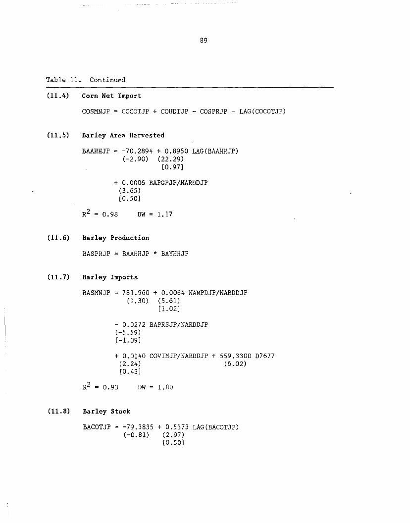
89
Table 11. Continued
(11.4) Corn Net Import
(11.5)
(11.6)
( 11. 7)
(11.8)
COSMNJP = COCOTJP + COUDTJP - COSPRJP - LAG(COCOTJP)
Barley Area Harvested
BAAHHJP = -70.2894 + 0.8950 LAG(BAAHHJP) (-2.90) (22.29)
[0. 97]
+ 0.0006 BAPGPJP/NARDDJP (3.65) [0. 50]
DW = 1.17
Barley Production
BASPRJP = BAAHHJP * BATrlHJP
Barley Imports
BASMNJP = 781.960 + 0.0064 NANPDJP/NARDDJP (1.30) (5.61)
[ l. 02]
- 0.0272 BAPRSJP/NARDDJP (-5.59) [-1.09]
+ 0.0140 COVIMJP/NARDDJP + 559.3300 D7677 (2.24) (6.02) [0.43]
R2 = 0.93 DW = l. 80
Barley Stock
BACOTJP = -79.3835 + 0.5373 LAG(BACOTJP) (-0.81) (2.97)
[0.50]
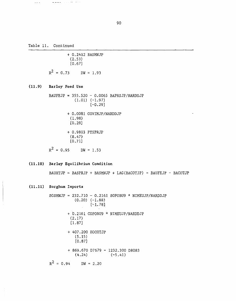
90
Table 11. Continued
(11.9)
+ 0.2412 BASMNJP (2.53) [0.67]
R2 = 0.73 DW = 1.93
Barley Feed Use
BAUFEJP = 355.520 - 0.0065 BAPRSJP/NARDOJP (1.01) (-1.97)
[-0.29]
+ 0.0081 COVIMJP/NARDOJP (1. 98) [0. 28]
+ 0.9803 PYSPRJP (8.47) [0.71]
OW = 1.53
(11.10) Barley Equilibrium Condition
BAUHTJP = BASPRJP + BASMNJP + LAG(BACOTJP) - BAUFEJP - BACOTJP
(11.11) Sorghum Imports
SGSMNJP = 232.710- 0.2161 SGPOBU9 * NIMEUJP/NARDDJP (0.20) (-1.88)
r~ L 78J
+ 0.2161 COPOBU9 * NIMEUJP/NARDDJP (2.17) [ 1. 87]
+ 407.200 HOCOTJP (5.15) [0. 87]
+ 869.670 07679 - 1232.300 08083 (4.24) (-5 .41)
OW= 2.20

91
Table 11. Continued
(11.12) Sorghum Stocks
SGCOTJP = -57.1494 + 0.5308 LAG(SGCOTJP) (-0.61) (2.74)
[0.52]
+ 0.0561 SGSMNJP (2.02) [0.65]
R2 = 0.62 DW = 2.01
(11.13) Sorghum Equilibrium Condition
SGUDTJP = SGSMNJP + LAG(SGCOTJP) - SGCOTJP
(11.14) Hog Inventories
HOCOTJP = -22.6137 + 0.5071 LAG(HOCOTJP) (-1.52) (2.78)
[ 0. 49]
- 0.00004 COVIMJP/NARDDJP (-2.75) [-0.17]
+ 2.3213 LOG(NANPDJP/NARDDJP) ( 1. 76)
(11.15) Poultry Production
PYSPRJP = -2520.170 + 0.7362 LAG(PYSPRJP) (-1.23) (5. 71)
[0. 68]
- 0,0035 COVIMJP/NARDDJP (-2.79) [-0.16]
+ 240.05 LOG(NANPJP/NARDDJP) ( 1. 38)

92
Table 11. Continued
(11.16) Feed-Grain Imports
FGSMNJP = COSMNJP + BASMNJP + OASMNJP
Endogenous Variables
BAAHHJP: BACOTJP: BASMNJP: BASPRJP: BAUFEJP: BAUHTJP: COCOTJP: COVIMJP: COSMNJP: COUDTJP: HOCOTJP: PYSPRJP: SGCOTJP: SGSMNJP: SGUDTJP:
Japan, barley area harvested, 1000 hectares Japan, barley ending stocks, 1000 metric tons Japan, barley net imports, 1000 metric tons Japan, barley.production, 1000 metric tons Japan, barley feed use, 1000 metric tons Japan, barley food use, 1000 metric tons Japan, corn ending stocks, 1000 metric tons Japan, corn import unit value, Yen/metric ton Japan, corn net imports, 1000 metric tons Japan, corn domestic use, 1000 metric tons Japan, hog inventories, January 1, million head Japan, poultry production, cal. year, 1000 metric tons Japan, sorghum ending stocks, 1000 metric tons Japan, sorghum net imports, 1000 metric tons Japan, sorghum domestic use, 1000 metric tons
Exogenous Variables
BAPGPJP: BAPRSJP: BAYHHJP: COPOBU9: COSPRJP: D73: D7677: D7679: 08083: DOPOPJP: NANPDJP: NARDDJP: NIMEUJP: RIUFEJP: SGPOBU9: SHIFT73: SHIFT74: SHIFT77: SHIFT79: SHIFT80:
Japan, barley government purchase price, Yen/metric ton Japan, barley resale price, Yen/metric ton Japan, barley yield per hectare, metric tons U.S., corn gulf port price, $/metric ton Japan, corn production, 1000 metric tons Dummy variable, 1 in 1973, 0 otherwise Dummy variable, 1 in 1976 and 1977, 0 otherwise Shift variable, 1 from 1976-79, 0 otherwise Shift variable, 1 from 1980-83, 0 otherwise Japan, population, million Japan, gross domestic product, billion Yen Japan, gross domestic product deflator, 1980=100 Japan, bilateral exchange rate, period average, Yen/$ Japan, rice feed use, 1000 metric tons U.S., sorghum gulf port price, $/metric ton Shift variable, 1 beginning in 1973, 0 otherwise Shift variable, 1 beginning in 1974, 0 otherwise Shift variable, 1 beginning in 1977, 0 otherwise Shift variable, 1 beginning in 1979, 0 otherwise Shift variable, 1 beginning in 1980, 0 otherwise

93
used as a feed in Japan, and here it is estimated that the crop has a nearly
one-for-one substitution effect with corn and is highly significant. Rice feeds
also have a substitution effect with corn. Although only a small amount of rice
is fed livestock each year, the coefficient is negative and significant.
Unlike rice, wheat, and barley, which in Japan are insulated from world
price fluctuations, corn enters the country freely. Because of this, corn
ending stocks are influenced by world price. Food security is still a
determining factor in the level ·of stocks held, however. With corn, stocks are
a combination of stocks held by formula feed processors and agricultural
cooperatives, and those held by the Formula Feed Supply Stabilization
Organization under a government-subsidized program.
The corn ending stocks equation (11.2) contains beginning stocks, real
corn-import unit value, and a shift variable beginning in 1973/74. The real
corn-import unit value has the expected negative coefficient but is not
significant. The shift variable reflects a combination of occurrences which
have led to increased stock levels in Japan. One of them was the reduction in
rice stocks in the early 1970s due to increased rice feeding. This reduction
not only resulted in increased competition for feed grains, but also left idle a
large amount of stockholding capacity. These effects would normally have been
fairly short lived, but they were followed by policies aimed at increasing
stocks beginning in 1976.
The corn-import unit value equation (11.3) is the price linkage between the
U.S. Gulf-port price for corn and the average value of corn imported into Japan.
It also contains a dummy variable for 1973--the first oil embargo. The
Gulf-port price in Yen is highly significant, and the elasticity indicates a
94
high degree of price transmission. The dummy variable for 1973/74 is negative,
implying that most corn purchases made by Japanese importers were made at lower
than the season average price. This variable is also significant. The Japanese
corn market is cleared through the net import identity (11.4).
There are four behavioral equations and two identities modeled for the
barley component of the Japanese feed-grains submodel. Barley area harvested
(11.5) is a function of the previous year area and of the real government
purchase price of barley. Barley policies are similar to those for wheat, with
the purchase price being set wel" above the world price to support barley
producers. Barley purchase price is set by the government before planting.
Because of this, current purchase price is used in the equation. The
coefficient of real purchase price has a positive sign and is significant.
Supply elasticity (0.50) is similar to estimates of 0.55 by Sullivan et al.
(1989) and of 0.6 by Tyers (1984) for "other coarse grains." Barley production
(11.6) is the product of barley area harvested and barley yield.
Barley imports are handled by the government food agency, as are imports of
wheat, thereby maintaining domestic policy prices. The barley net imports
equation (11.7) contains real income, real barley resale price, real corn-import
unit value, and a shifter for 1976-77. Real barley resale price has the
anticipated sign and is highly significant. Estimated elasticity is high
compared to that determined by other studies, but it is for barley imports, not
for total consumption. Tyers estimated the total coarse grain (including corn)
demand elasticity to be -0.6. The corn-import unit value was used because corn
enters Japan freely, and this price should be reflected in the price paid by
feed producers. The coefficient is positive, indicating that corn is a

95
competing feed. The cross-price elasticity (0.43) is higher than the value of
0.20 found in Sullivan et al., but it is still fairly low.
Most barley imported into Japan is used for livestock feed. As incomes
increase in Japan, meat and livestock products consumption is also increasing,
which implies a positive and fairly substantial effect on barley imports. The
coefficient for real income is positive and significant at the 5-percent level.
Income elasticity is similar to the estimate of 0.96 in Tyers for total coarse
grains.
The shifter for 1976/77 takes into account the stock-building programs
begun in 1976. For barley, there was a two-year buildup of stocks. This
variable has the expected sign and is highly significant.
The Japanese government has a buffer-stocks policy for feed as well as for
food grains. The specification for the barley-stocks equation (11.8) is similar
to that for wheat stocks. Beginning stocks represent an adjustment toward a
desired level of buffer stocks, whereas net imports represent transaction
demand. Both have the expected positive signs and are significant at the
5-percent level.
Barley utilization is subdivided into feed and food uses. Feed use (11.9)
is dependent upon barley resale price, corn-import unit values, and livestock
numbers. The real barley resale price has a negative coefficient as expected,
but it is not significant. Corn is a substitute in feed rations for barley.
The corn-import unit value is used to capture these substitution effects. The
coefficient has the expected positive sign but is not significant at the
5-percent level. Barley is fed to poultry in Japan; poultry production is used
in this equation and is highly significant with the anticipated positive sign.

96
Barley food use is the market clearing identity. Food use is the residual
of government managed supply and stock changes, and feed use is the residual of
the livestock industry.
There is no sorghum production in Japan, so all demand for this grain must
be met by imports. The sorghum component consists of two behavioral equations
and of one identity.
Because Japan does not produce sorghum, imports of this grain reflect the
country's internal demand conditions. Sorghum imports (11.11) are a function of
both sorghum price on the world market and corn price on the world market
because there are no import barr~ers against these two grains entering Japan.
Imports are also affected by hog inventories. During the period 1976-79,
sorghum imports were well above normal levels, corresponding to a period of
rapid increase in livestock production. During the early 1980s, livestock
production slowed as markedly as it had increased in the late 1970s, and sorghum
imports declined. The real sorghum Gulf-port price in Yen, per metric ton, is
used as the world price affecting Japanese imports. The real corn Gulf-port
price in Yen, per metric ton, is also used as the world price of the competing
imported feed grain. Both variables have the expected sign, but neither is
significant at the 5-percent level. The most significant variable in the import
equation is hog inventories. The estimated elasticity is only slightly less
than unity, indicating that sorghum use in Japan closely follows hog production.
The two shift variables are significant and represent the sharper-than-normal
increases and decreases in livestock production over their respective periods.
As with other grains, there is a minimum level of buffer stocks of sorghum
which the government subsidizes. Formula-feed processors and cooperatives hold

97
these stocks, as they do corn, in addition to their private reserves. The
specification for the sorghum ending stocks equation (11.12) includes beginning
stocks and sorghum imports. As with other grain stocks, beginning stocks and
imports represent an adjustment toward a desired level of stocks and transaction
demands, respectively. Both variables have the expected positive signs and are
significant.
The Japanese sorghum market is cleared through the sorghum-use identity
( 11. 13) • Sorghum use is equal to sorghum imports-· less the annual change in
stock level.
The simple livestock equaticns in this submodel are not meant to capture
cycles, but merely to mimic long-term growth rates in livestock production and
to reflect income and certain input effects.
The hog inventory equation (11.14) consists of a one-year lag of the
dependent variable, the real corn-import unit value, and the log of real income.
The lagged dependent variable implies that current hog numbers depend, in part,
upon the previous year's hog numbers. This variable has a positive sign and is
significant at the 5-percent level. The corn-import unit value represents the
effects of input prices. It is expected that, as inputs become more expensive,
fewer animals will be kept. The sign on this variable is negative and
significant. The estimated elasticity (-0.17) is slightly above the very low
estimate of -0.07 determined by Sullivan et al. The log of real income is
positive, as expected.
The poultry production equation (11.15) is specified similarly to the hog
inventory equation. The lagged dependent variable is the most significant
variable in the equation. The corn-import unit value is negative and

98
significant, and estimated elasticity is the same as the -0.16 found in
Sullivan et al. The log of real income is positive but not significant at the
5-percent level.
Feed-grain imports are described by identity (11.16) as the sum of imports
of corn, barley, and oats.
Brazilian Submodel
The Brazilian component of the feed-grains model is reported in Table 12.
For Brazil, three feed grains--corn, barley, and oats--are combined and modeled
as one commodity. Feed-grain area harvested (12.1) is estimated as a function
of real barley price, wheat price, soybean price, lagged acreage, and dummy
variables. Because wheat and soybeans are competing crops, the prices of these
two crops enter the area harvested equation. Own-price supply elasticity is
0.29, and cross-price elasticities are -0.28 (wheat) and -0.16 (soybean).
Feed-grain yield is exogenous in the model. Feed-grain production (12.2) is
described by the identity as acreage times yield.
On the demand side, only domestic use (12.3) is estimated. The explanatory
variables in the domestic use. equation are real income, real corn price, and
dummy variables. Own-price elasticity is -0.13 and income elasticity is 0.49.
Feed-grain imports are described by the identity as domestic use minus domestic
supply. Three price-linkage equations for corn, wheat, and soybeans are
estimated. Price-transmission elasticities for corn, wheat, and soybeans are
0.52, 0.1, and 0.72, respectively.
Mexican Submodel
For Mexico, supply and use equations for feed grains (corn, barley, and
oats) and sorghum are estimated. The estimated equations are presented in Table
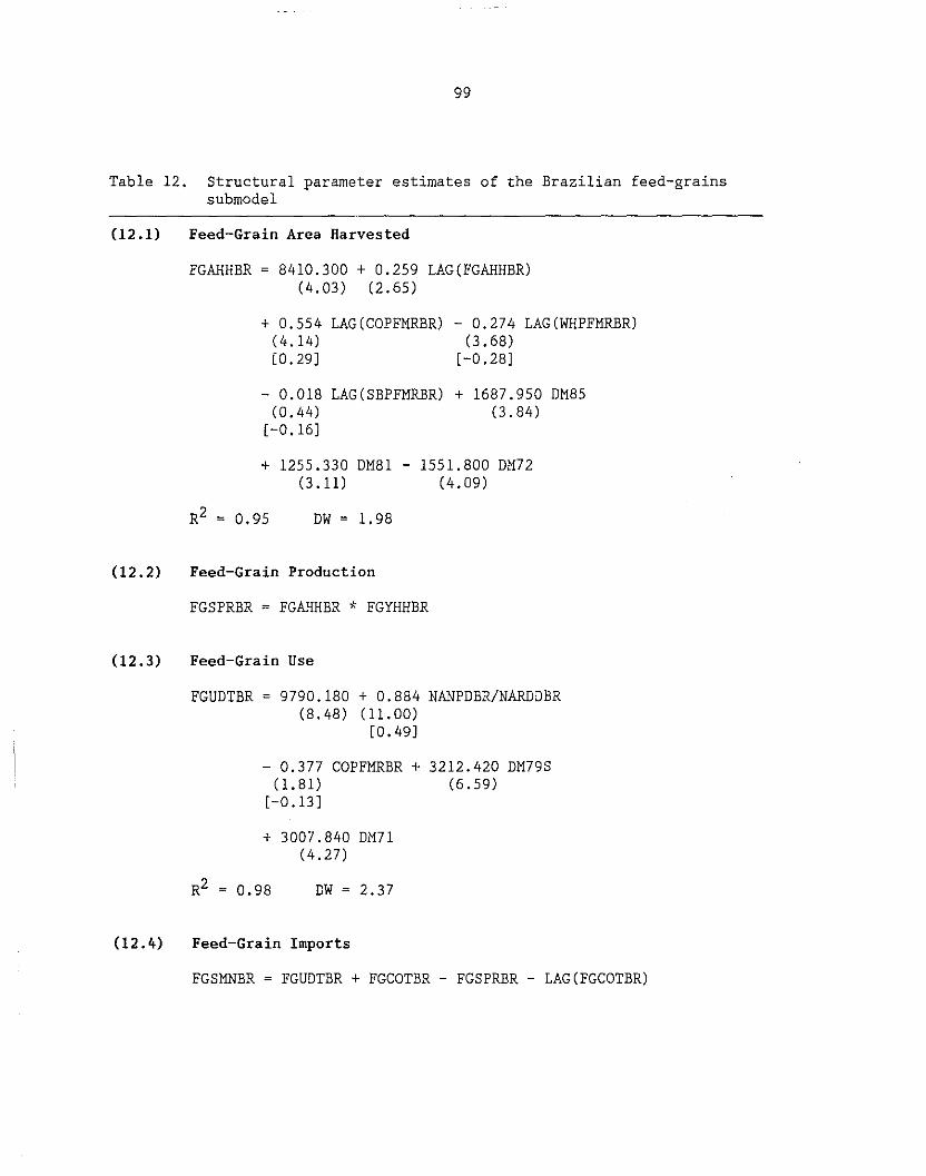
99
Table 12. Structural parameter estimates of the Brazilian feed-grains submodel
(12.1) Feed-Grain Area Harvested
(12. 2)
(12.3)
(12.4)
FGAHHBR = 8410.300 + 0.259 LAG(FGAHHBR) (4.03) (2.65)
+ 0.554 LAG(COPFMRBR) (4.14) [0.29]
- 0.018 LAG(SBPFMRBR) (0.44)
[-0.16]
- 0.274 LAG(WHPFMRBR) ( 3. 68)
[-0.28]
+ 1687.950 DM85 ( 3. 84)
+ 1255.330 DM81 - 1551.800 DM72 (3.11) (4.09)
R2 = 0 95 . DW = 1. 98
Feed-Grain Production
FGSPRBR = FGAHHBR * FGYHHBR
Feed-Grain Use
FGUDTBR = 9790.180 + 0.884 NANPDBR/NARDDBR (8.48) (11.00)
[0.49]
- 0.377 COPFMRBR + 3212.420 DM79S (1.81) (6.59)
[-0.13]
+ 3007.840 DM71 (4.27)
R2 0. 98 DW = 2.37
Feed-Grain Imports
FGSMNBR = FGUDTBR + FGCOTBR - FGSPRBR - LAG(FGCOTBR)
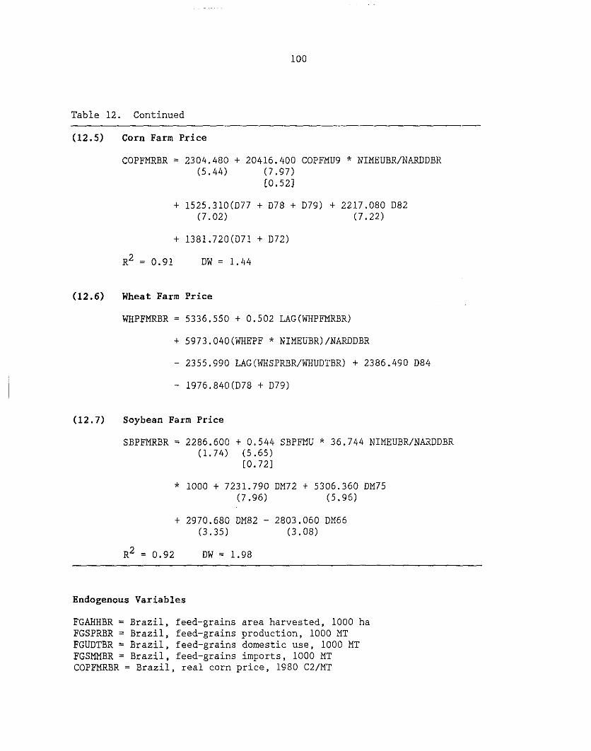
100
Table 12. Continued
(12.5) Corn Farm Price
COPFMRBR ~ 2304.480 + 20416.400 COPFMU9 * NIMEUBR/NARDOBR (5.44) (7.97)
[0.52]
+ 1525.310(077 + 078 + 079) + 2217.080 082 (7.02) (7.22)
+ 1381.720(071 + 072)
OW ~ 1. 44
(12.6) Wheat Farm Price
(12. 7)
WHPFMRBR ~ 5336.550 + 0.502 LAG(WHPFMRBR)
+ 5973.040(WHEPF * NIMEUBR)/NARDOBR
- 2355.990 LAG(WHSPRBR/WHUOTBR) + 2386.490 084
- 1976.840(078 + 079)
Soybean Farm Price
SBPFMRBR ~ 2286.600 + 0.544 SBPFMU * 36.744 NIMEUBR/NARDOBR (1.74) (5.65)
[0.72]
* 1000 + 7231.790 OM72 + 5306.360 OM75 (7.96) (5.96)
+ 2970.680 OM82 - 2803.060 OM66 (3.35) (3.08)
OW ~ 1.98
Endogenous Variables
FGAHHBR ~ Brazil, feed-grains area harvested, 1000 ha FGSPRBR ~ Brazil, feed-grains production, 1000 MT FGUOTBR ~ Brazil, feed-grains domestic use, 1000 MT FGSMMBR ~ Brazil, feed-grains imports, 1000 MT COPFMRBR ~ Brazil, real corn price, 1980 C2/MT
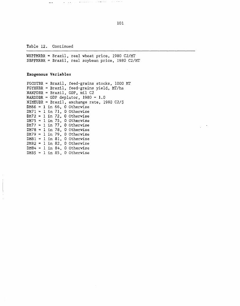
Table 12.
WHPFMRBR SBPFMRBR
101
Continued
=Brazil, real wheat price, 1980 C2/MT Brazil, real soybean price, 1980 C2/MT
Exogenous Variables
FGCOTBR Brazil, feed-grains stocks, 1000 MT FGYHHBR = Brazil, feed-grains yield, MT/ha NANPDBR Brazil, GDP, mil C2 NARDDBR = GDP deplator, 1980 = 1. 0 NIMEUBR = Brazil, exchange rate, 1980 C2/$ DM66 1 in 66, 0 Otherwise DM71 = 1 in 71, 0 Otherwise DM72 = 1 in 72, 0 Otherwise DM75 = 1 in 75, 0 Otherwise DM77 = 1 in 77, 0 Otherwise DM78 = 1 in 78, 0 Otherwise DM79 = 1 in 79, 0 Otherwise DM81 1 in 81, 0 Otherwise DM82 = 1 in 82, 0 Otherwise DM84 1 in 84, 0 Otherwise DM85 = 1 in 85, 0 Otherwise

102
Table 13. Structural parameter estimates of the Mexican feed-grains submodel
(13.1) Feed-Grain Production
( 13. 2)
(13.3)
(13.4)
( 13. 5)
FGSPRMX = -8433.290 + 9415.450 FGYHHMX + 0.748 LAG(FGAHHMX) (4.60) (15.26) (4.60)
- 1921.540(082 + 084) (6.38)
+ 0.198 LAG(COPFMMXR) (1.41) [0. 08]
OW= 2.33
Feed-Grain Area Harvested
FGAHHMX = FGSPRMX/FGYHHMX
Feed-Grain Domestic Use
FGUOTMX = 8866.240 (3.96)
- 2536.480 COPFMMXR/WHPFMMXR ( 1. 09)
[-0.28]
+ 7.042 POSPRMX + 1777.270 077 + 1952.300(080 + 081) (6.55) (2.05) (3.23)
R2 = 0.90 DW = 2.04
Feed-Grain Stocks
FGCOTMX = -1360.420 + 0.215 LAG(FGCOTMX) (3.94) (2.21)
+ 0.197 FGSPRMX (4.97) [2. 86]
+ 1233.340 080 - 623.537 078 - 473.300 D84 (5.81) (2.97) (2.27)
R2 = 0.90 OW= 1.93
Corn Farm Price
COPFMMXR = 2536.360 + 0.315 LAG(COPFMMXR) (2.61) (1.87)
+ 8.094 COPFMU9 ( 1. 49) [0.16]
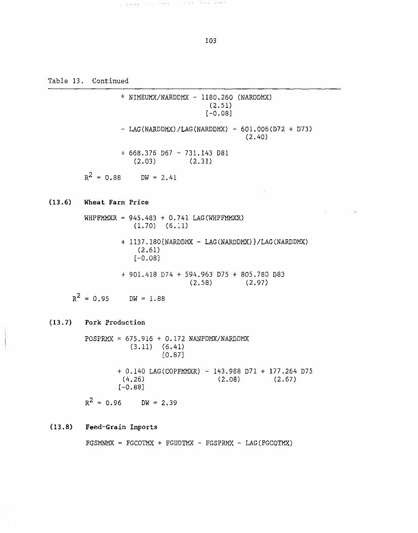
103
Table 13. Continued
* NIMEUMX/NARDDMX - 1180.260 (NARDDMX) (2.51)
[-0.08)
- LAG(NARDDMX)/LAG(NARDOMX) - 601.006(072 + 073) (2.40)
+ 668.376 067- 731.143 081 (2.03) (2.31)
R2 = 0. 88 ow = 2.41
(13.6) Wheat Farm Price
WHPFMMXR = 945.483 + 0.741 LAG(WHPFMMXR) (1.70) (6.d)
R2 = 0.95
+ 1137.180[NARDDMX- LAG(NARDOMX))/LAG(NARDOMX) (2.61)
[-0.08]
+ 901.418 074 + 594.963 075 + 805.780 D83 (2.58) (2.97)
ow= 1.88
(13.7) Pork Production
POSPRMX = 675.916 + 0.172 NANPDMX/NARDDMX (3.11) (6.41)
[0.87)
+ 0.140 LAG(COPFMMXR) - 143.988 D71 + 177.264 075 (4.26) (2.08) (2.67)
[-0.88]
R2 = 0.96 ow = 2.39
(13.8) Feed-Grain Imports
FGSMNMX = FGCOTMX + FGUOTMX - FGSPRMX - LAG(FGCOTMX)

104
Table 13. Continued
* NIMEUMX/NARDDMX- 1180.260 (NARDDMX) (2.51)
(-0.08]
- LAG(NARDDMX)/LAG(NARDDMX) - 601.006(072 + D73) (2.40)
+ 668.376 067- 731.143 D81 (2.03) (2.31)
R2 = 0. 88 DW = 2.41
(13.6) Wheat Farm Price
WHPFMMXR = 945.483 + 0.741 LAG(WHPFMMXR) (1.70) (6.11)
R2 = 0.95
+ 1137.180(NARDDMX- LAG(NARDDMX)]/LAG(NARDDMX) (2.61)
(-0.08]
+ 901.418 D74 + 594.963 D75 + 805.780 D83 (2.58) (2.97)
DW = 1.88
(13.7) Pork Production
POSPRMX = 675.916 + 0.172 NANPDMX/NARDDMX (3.11) (6.41)
(0.87]
+ 0.140 LAG(COPFMMXR) - 143.988 D71 + 177.264 D75 (4.26) (2.08) (2.67)
(-0.88]
R2 = 0.96 DW = 2.39
(13.8) Feed-Grain Imports
FGSMNMX = FGCOTMX + FGUDTMX - FGSPRMX - LAG(FGCOTMX)

Table 13. Continued
(13.13) Sorghum Farm Price
SGPFMMXR = 2292.740 (9.97)
+ 0.004 (5.37) [ 0. 42]
105
SGPFMU9 * NIMEUMX/NARDDMX
- 2157.700[NARDDMX- LAG(NARDDMX)]/LAG(NARDDMX) (14.40) [-0.18]
- 545.397 D73 + 468.452 D75 (3.45) (3.10)
R2 = 0.96 DW = 1. 65
(13.14) Sorghum Imports
SGSMNMX = SGUDTMX + SGCOTMX - SGSPRMX - LAG(SGCOTMX)
Endogenous Variables
FGSPRMX Mexico, Feed-Grain Production, 1000 MT FGAHHMX = Mexico, Feed-Grain Area Harvested, 1000 ha FGUDTMX Mexico, Feed-Grain Domestic Use, 1000 MT COPFMMXR = Mexico, Corn Farm Price, 1980 pesos/MT WHPFMMXR = Mexico, Wheat Farm Price, 1980 pesos/MT POSPRMX Mexico, Pork Production, 1980 pesos/MT FGCOTMX Mexico, Feed-Grain Stocks, 1000 MT FGSMNMX = Mexico, Feed-Grain Imports, 1000 MT SGAHHMX Mexico, Sorghum Area Harvested, 1000 ha SGSPRMX Mexico, Sorghum Production, 1000 MT SGUDTMX Mexico, Sorghum Domestic Use, 1000 MT SGCOTMX Mexico, Sorghum Stocks, 1000 MT SGPFMMXR = Mexico, Sorghum Farm Price
Exogenous Variables
FGYHHMX NARDDMX NIMEUMX NANPDMX D67 = 1 D71 = 1 D72 1
Mexico, Feed-Grain Yield, MT/ha Mexico, GDP Deflator, 1980 = 1.0
= Mexico, Exchange Rate, pesos 1$ = Mexico, GDP, mil pesos in 1967 and 0 Otherwise in 1971 and 0 Otherwise in 1972 and 0 Otherwise

106
Table 13. Continued
D73 1 in 1973 and 0 Otherwise D74 1 in 1974 and 0 Otherwise D75 1 in 1975 and 0 Otherwise D77 = 1 in 1977 and 0 Otherwise D78 = 1 in 1978 and 0 Otherwise D79 1 in 1979 and 0 Otherwise D80 1 in 1980 and 0 Otherwise D81 1 in 1981 and 0 Otherwise D82 = 1 in 1982 and 0 Otherwise D83 1 in 1983 and 0 Otherwise D84 = 1 in 1984 and 0 Otherwise

107
13. Feed-grain production (13.1) is endogenously estimated as a function of
real corn farm price, feed-grain yield, lagged acreage, and dummy variables.
Estimated supply-price elasticity is 0.08. Feed-grain area harvested (13.2) is
derived by dividing production by yield. Feed-grain domestic use (13.3) is
estimated as a function of the ratio of corn farm price to wheat farm price,
pork production, and dummy variables. Own-price demand elasticity is estimated
at -0.28, and cross-price demand elasticity is restricted at 0.28. Poultry
production is significant in explaining the variation in feed-grain domestic
use. The explanatory variables ~n the stock equation (13.4) are production, lag
stocks, and dummy variables.
Corn farm price (13.5) is linked to U.S. corn farm price. Price
transmission elasticity is 0.16. Other explanatory variables in the price
linkage equation are lagged corn farm price, inflation, and dummy variables.
Wheat farm price (13.6) is estimated as a function of lagged wheat farm price,
inflation, and dummy variables.
Because pork production (13.7) is one of the explanatory variables in the
domestic feed-grain use equation, it is endogenously estimated as a fuuction of
real corn farm price and real income. Input-price elasticity is estimated at
-0.88. Feed-grain imports are described by the identity (13.8) as domestic
demand minus domestic supply.
In contrast with the feed-grains component, the sorghum area component
(13.9) is endogenously estimated. The explanatory variables in this equation
are real sorghum farm price, real wheat farm price, lagged sorghum acreage, and
dummy variables. Own-price supply elasticity is 0.66 and cross-price elasticity
is 0.80. Sorghum production (13.10) is the product of area times yield.

108
Sorghum domestic use (13.11) is estimated as a function of real sorghum price,
real income, and sorghum imports. Own-price demand elasticity is -0.60. The
important explanatory variable in the sorghum stock equation (13.12) is
production. Sorghum farm price (13.13) is linked to the U.S. farm price.
Price-transmission elasticity is 0.42. Sorghum imports are described by
identity (13.14) as domestic demand minus domestic supply.
Egyptian Subrnodel
Only corn is modeled for Egypt (see Table 14). On the supply side, corn
production (14.1) is endogenously estimated. The explanatory variables in corn
production are real corn farm price, real wheat farm price, lagged production,
corn yield, and dummy variables. Because wheat is a competing crop, wheat farm
price is used to capture the cross-price effect on corn production. Corn-price
elasticity is 0.11 and the wheat price elasticity is -0.07. Corn yield is
exogenous in the model. Corn area harvested (14.2) is described as production
divided by yield.
On the demand side, corn domestic use and stocks are endogenously
estimated. Because corn domestic use (14.3) is constrained by production,
production is one of the explanatory variables in the domestic use equation.
Other explanatory variables are real income and dummy variables. Corn stocks
(14.4) are estimated as a function of corn farm price, production, and dummy
variables. Price elasticity of stock demand is estimated at -0.24. Corn farm
price (14.5) is linked to U.S. farm price. Price-transmission elasticity is
0.70. Corn imports (14.6) are equal to domestic demand minus domestic supply.
Feed-grain imports (14.7) are determined as the sum of corn and barley imports.

109
Table 14o Structural parameter estimates of the Egyptian feed-grains submodel
(14o1) Corn Production
( 14 0 2)
(14o3)
( 14 0 4)
COSPREG = -634o338 + Oo760 LAG(COSPREG) + 321o735 COYHHEG (1.03) (6o00) (2o44)
+ 336o531 Clo 25) [Ooll]
- 256o604 (Oo65)
[-Oo07l
LAG(COPFMEG/NARDDEG)
LAG(WHPFMEG/NARDDEG) + 323o852 DM178 (2o99)
+ 240o775 DM180 ( 2 0 18)
DW = 2o07
Corn Area Harvested
COAHHEG = COSPREG/COYHHEG
Corn Domestic Use
COUDTEG = -468o468 + 12o065 NANPDEG/NARDDEG (Oo62) (2057)
[ 0 0 46]
+ 1271ol00 DM184 + Oo805 COSPREG- 257o171 D79 (6o23) (1.66) (1.24)
[Oo65]
+ 565o047 D85 (2o85)
R2 = Oo99 DW = 1.59
Corn Stocks
COCOTEG = 1298o830 - 598o080(COPFMEG/NARDDEG) * SHIFT73 (52o09) (4o43)
[ -Oo 24]
+ Oo347 COSPREG * SHIFT73 - 370o817 DM179 (7o62) (5o47l

110
Table 14. Continued
- 190.284(DM177 + DM176)
0.95 DW = l. 99
(14.5) Corn Farm Price
COPFMEG = -133.801 + (2.98)
40.817 (4.92) [0.70]
COPFMU9 * NIMEUEG
+ 134.098 (2.98) [2.42]
LAG(COUDTEG/COSPREG) - 23.663 DM178 ( l. 82)
0.92 DW = 1.35
(14.6) Corn Imports
COSMNEG = COUDTEG + COCOTEG - COSPREG - LAG(COCOTEG)
(14 0 7) Feed-Grain Imports
FGSMNEG = COSMNEG + BASMNEG
Endogenous Variables
COSPREG Egypt, Corn Production, 1000 MT COAHHEG = Egypt, Corn Area Harvested, 1000 ha COUDTEG = Egypt, Corn Domestic Use, 1000 MT COCOTEG Egypt, Corn Stocks, 1000 MT COPFMEG = Egypt, Corn Farm Price, pounds/MT COSMNEG Egypt, Corn Imports, 1000 MT FGSMNEG = Egypt, Feed-Grain Imports, 1000 MT
Exogenous Variables
COYHHEG Egypt, Corn Yield, MT/ha NARDDEG = Egypt, GDP Deflator, 1980=100 WHPFMEG Egypt, Wheat Farm Price, pounds/MT NANPDEG =Egypt, GOP, mil.pounds NIMEUEG = Egypt, Exchange Rates 079 = 1 in 1979 and 0 Otherwise

111
Table 14. Continued
D85 = 1 in 1985 and 0 Otherwise D176 = 1 in 1976, 0 Otherwise D177 1 in 1977. 0 Otherwise D178 = 1 in 1978, 0 Otherwise D179 1 in 1979, 0 Otherwise D184 1 in 1984, 0 Otherwise SHIFT73 = 1 after 1972, 0 Otherwise

112
Indian Submodel
Only sorghum is modeled in the submodel for India (see Table 17). Sorghum
area harvested (15.1) is specified as a function of real per acre returns from
the sorghum crop, real per acre returns from the wheat crop, lagged acreage, and
dummy variables. Wheat is the competing crop for sorghum. Own-price elasticity
is 0.11 and cross-price elasticity is -0.18. Sorghum production (15.2) is
defined as acreage times yield.
On the demand side, sorghum domestic use and stocks are endogenously
estimated. Sorghum production is an important variable in explaining the
variation in sorghum use (15.3). Explanatory variables in the sorghum stocks
equation (15.4) are production, lag stocks, and dummy variables. Variation in
real sorghum price (15.5) is explained by the ratios of sorghum production to
use, lagged price, ann dummy variables. Sorghum imports (15.6) are described as
domestic demand minus domestic supply.
Nigerian Submodel
Only sorghum is modeled in the Nigerian submodel (see Table 16). Sorghum
area harvested (16.1) is estimated as a function of sorghum farm price, corn
farm price, lagged acreage, and dummy variables. Own-price supply elasticity is
estimated at 0.57, and cross-price elasticity is restricted at -0.57. Sorghum
production (16.2) is described as acreage times yield.
On the demand side, only sorghum use is estimated. The explanatory
variables in the sorghum-use equation (16.3) are real sorghum price and
production. Own-price demand elasticity is -0.003. Variation in the sorghum
price (16.4) is captured by the ratio of production to use, GDP deflator, and

113
Table 15. Structural parameter estimates of the Indian feed-grains submodel
(15.1) Sorghum Area Harvested
(15.2)
(15.3)
(15.4)
SGAHHIN = 14200.100 + 0.218 LAG(SGAHHIN) (8.05) (2.06)
+ 2.895 LAG[(SGPFMIN/NARDOIN) * SGYHHIN] (4.31) [0. 11]
+ 1162.740(068 + 069) (4.31)
- 1.433 LAG[(WHPFMIN/NARDOIN) * WHYHHIN] (4.62)
[-0.18]
- 1652.700 074 + 700.813 079- 1147.010 072 (2.51) (4.13)
DW = 1.98
Sorghum Production
SGSPRIN = SGAHHIN * SGYHHIN
Sorghum Domestic Use
SGUOTIN = 1277.310 + 0.892 (2. 72) (19.68)
[0.87]
SGSPRIN + 643.314(067 + 068 + 069) ( 3. 63)
OW= 1.92
Sorghum Stocks
SGCOTIN = 59.918 + 0.293 LAG(SGCOTIN) (0.39) (5.02)
+ 0.032 SGSPRIN (2.10) [0.42]
+ 763.250 077 + 325.024(073 + D74 + D75 + 076) (8.15) (6.60)
+ 336.723 078 ( 3. 44)
OW= 2.10

114
Table 15. Continued
(15.5) Sorghum Real Price
SGPFMIN = 1953.370 + 0.861 LAG(SGPFMIN) (2.65) 02.39)
- 1894.350 (2.68)
[-1. 76]
SGSPRIN/SGUDTIN + 179.487 D71 - 448.156 D74 ( 1. 80) (4. 28)
R2 = 0.96 DW = 2.49
(15. 6) Sorghum Imports
SGSMNIN = SGUDTIN + SGCOTIN - SGSPRIN - LAG(SGCOTIN)
Endogenous Variables
SGAHHIN = India, Sorghum Area Harvested, 1000 ha SGSPRIN India, Sorghum Production, 1000 MT SGPFMIN India, Sorghum Farm Price, rupees/MT SGUDTIN India, Sorghum Domestic Use, 1000 MT SGCOTIN India, Sorghum Stocks, 1000 MT SGSMNIN = India, Sorghum Imports, 1000 MT
Exogenous Variables
SGYHHIN = India, Sorghum Yield, MT/ha NARDDIN India, GDP Deflator, 1980=1. 0 WHPFMIN India, Wheat Farm Price, rupees/MT WHYHHIN India, Wheat Yield, MT/ha D67 1 in 1967 and 0 Otherwise D68 = 1 in 1968 and 0 Otherwise D69 1 in 1969 and 0 Otherwise D71 1 in 1971 and 0 Otherwise D72 1 in 1972 and 0 Otherwise D73 = 1 in 1973 and 0 Otherwise D74 1 in 1974 and 0 Otherwise D75 1 in 1975 and 0 Otherwise D76 = 1 in 1976 and 0 Otherwise D77 1 in 1977 and 0 Otherwise D79 = 1 in 1979 and 0 Otherwise
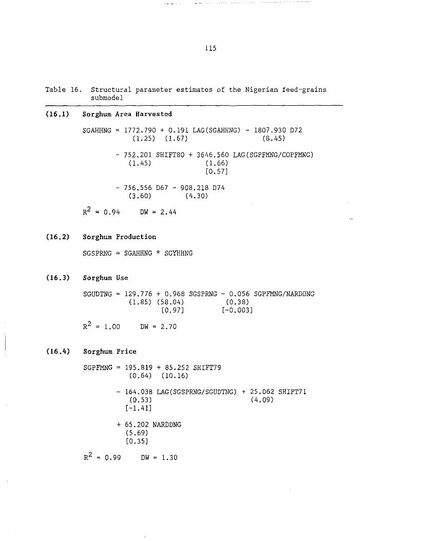
115
Table 16. Structural parameter estimates of the Nigerian feed-grains submodel
(16.1) Sorghum Area Harvested
(16. 2)
(16. 3)
(16.4)
SGAHHNG = 1772.790 + 0.191 LAG(SGAHHNG) - 1807.930 D72 (1.25) (1.67) (8.45)
- 752.201 SHIFT80 + 3646.560 LAG(SGPFMNG/COPFMNG) (1.45) (1.66)
[0.57]
- 756.556 D67 - 908.218 D74 (3.60) (4.30)
R2 = 0.94 DW = 2.44
Sorghum Production
SGSPRNG = SGAHHNG * SGYHHNG
Sorghum Use
SGUDTNG = 129.776 + 0.968 (1.85) (58.04)
[0.97]
SGSPRNG - 0.056 SGPFMNG/NARDDNG (0.38)
1.00 DW = 2.70
Sorghum Price
SGPFMNG = 195.819 + 85.252 SHIFT79 (0.64) (10.16)
[-0.003]
- 164.038 LAG(SGSPRNG/SGUDTNG) + 25.062 SHIFT71 (0.53) (4.09)
[-1.41]
+ 65.202 NARDDNG (5.69) [0.35]
DW = 1.30
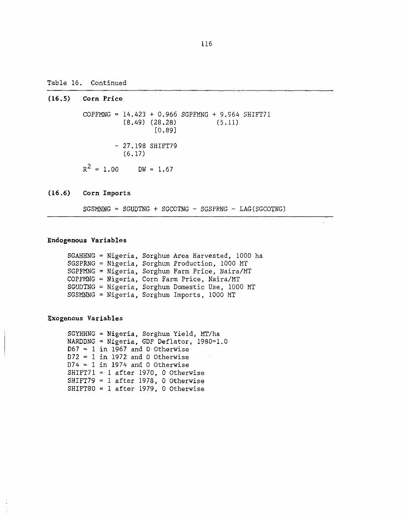
116
Table 16. Continued
(16.5) Corn Price
COPFMNG = 14.423 + 0.966 (8.49) (28.28)
[0.89]
SGPFMNG + 9.964 SHIFT71 (5.11)
- 27.198 SHIFT79 (6.17)
1.00 DW 1.67
(16 .6) Corn Imports
SGSMNNG = SGUDTNG + SGCOTNG - SGSPRNG - LAG(SGCOTNG)
Endogenous Variables
SGAHHNG SGSPRNG SGPFMNG COPFMNG SGUDTNG SGSMNNG
Nigeria, Sorghum Area Harvested, 1000 ha Nigeria, Sorghum Production, 1000 MT Nigeria, Sorghum Farm Price, Naira/MT Nigeria, Corn Farm Price, Naira/MT Nigeria, Sorghum Domestic Use, 1000 MT Nigeria, Sorghum Imports, 1000 MT
Exogenous Variables
SGYHHNG NARDDNG D67 = 1 D72 = 1 D74 = 1 SHIFT71 SHIFT79 SHIFT80
= Nigeria, Sorghum Yield, MT/ha = Nigeria, GDP Deflator, 1980=1.0 in 1967 and 0 Otherwise in 1972 and 0 Otherwise in 1974 and 0 Otherwise
1 after 1970, 0 Otherwise 1 after 1978, 0 Otherwise 1 after 1979, 0 Otherwise

117
and dummy variables. Corn farm-price (16.5) is endogenously estimated as a
function of sorghum farm-price and dummy variables. Corn imports (16.6) are
described as domestic demand minus domestic supply.
Saudi Arabian Submodel
In Table 17, which describes the Saudi feed-grains submodel, barley
domestic use (17.1) is endogenously estimated as a function of egg production
and a dummy variable. Because barley is a major feed used in egg production,
egg production is used as an explanatory variable in the barley domestic use
equation. Egg production (17.2) is also endogenously estimated as a function of
real income, crude-oil price, lagged egg production, and dummy variables.
Barley imports (17.3) are described as domestic use minus domestic supply.
Feed-grain imports (17.4) are defined as barley imports plus corn imports.
High-Income East Asian Submodel
Three behavioral equations--area harvested, domestic use, and stocks--are
endogenously estimated in the high-income East Asia submodel, which is
illustrated in Table 18. The explanatory variables in the area harvested
equation (18.1) are real U.S. corn price expressed in local currencies, lagged
acreage, and dummy variables. Supply-price elasticity is 0.27. Production
(18.2) is described as acreage times yield.
Feed-grain domestic use (18.3) is estimated as a function of corn price and
income. Demand is inelastic at -0.09, and income elasticity is close to unity.
Stocks (18.4) are estimated as a function of corn price, production, and lag
stocks. Feed-grain imports (18.5) are described as domestic demand minus
domestic supply.

118
Table 17. Structural parameter estimates of the Saudi Arabian feed-grains submodel
(17.1) Barley Domestic Use
(17. 2)
(17.3)
(17. 4)
BAUDTSA = -866.522 + 3.453 EGSPRSA + 921.522 SHIFT74 (6.44) (27 .61) (5. 75)
R2 = 0.99 DW = 1.47
Egg Production
EGSPRSA = -118.971 + 0.685 LAG(EGSPRSA) (1.15) (7.76)
+ 4.699 SHIFT82 * LTARCRUD * NIMEUSA/NARDDSA ( 5. 44)
+ 201.016 081 - 260.198 082 - 162.801 079 (4.89) (5.78) (4.71)
+ 0.001 SHIFT75 * NANPDSA/NARDDSA + 118.971 * SHIFT74 (2.92)
1.00 DW = 2.35
Barley Imports
BASMNSA = BAUDTSA + BACOTSA - BASPRSA - LAG(BACOTSA)
Feed-Grain Imports
FGSMNSA = BASMNSA + COSMNSA
Endogenous Variables
BAUDTSA = EGSPRSA BASMNSA = FGSMNSA =
Saudi Arabia, Saudi Arabia, Saudi Arabia, Saudi Arabia,
Exogenous Variables
Barley Domestic Use, 1000 MT Egg Production, mil pieces Barley Imports, 1000 MT Feed-Grain Imports, 1000 MT
LTARCRUD = Saudi Arabia, Crude Oil Price, $/bbl NIMEUSA = Saudi Arabia, Exchange Rate, Riyals/$
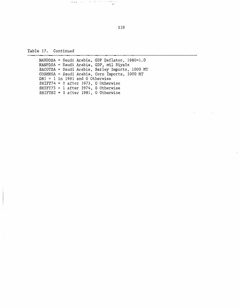
119
Table 17. Continued
NARDDSA Saudi Arabia, GDP Deflator, 1980=1. 0 NANPDSA Saudi Arabia, GDP, mil Riyals BACOT SA Saudi Arabia, Barley Imports, 1000 MT COSMNSA Saudi Arabia, Corn Imports, 1000 MT 081 = 1 in 1981 and 0 Otherwise SHIFT74 1 after 1973' 0 Otherwise SHIFT75 1 after 1974, 0 Otherwise SHIFT82 = 1 after 1981, 0 Otherwise

120
Table 18. Structural parameter estimates of the high-income East Asian feed-grains submodel
(18.1) Feed-Grain Area Harvested
(18.2)
(18.3)
(18.4)
FGAHHR4 ~ -85.308 + 0,848 LAG(FGAHHR4) (2.07) (13,50)
+ 48.692 LAG(CORPF/NARDDU9 (3.31)
* NIMERUUS) - 196.049 D76 (5.26)
[0. 27]
- 96.520 D85 (2.54)
DW ~ 1.93
Feed-Grain Production
FGSPRR4 ~ FGAHHR4 * FG~HR4
Feed-Grain Domestic Use
FGUDTR4 ~ 494.539 - 159.844 CORPF/NARDDU9 * NIMERUUS (0.96) (1.40)
[-0.09]
+ 46,511 NARPDR4$ + (26.56)
1111.520(078 + D82) - 818.368 D85 (4.68) (2.42)
[0. 99]
R2 0. 99 DW ~ 1. 64
Feed-Grain Stocks
FGCOTR4 ~ -448.384 + 0,782 LAG(FGCOTR4) (1,67) (7.70)
- 13.654 CORPF/NARDDU9 NIMERUUS (0.18)
[-0.03]
DW ~ 1. 71
+ 0.544 FGSPRR4 (3.33) [0.60]

121
Table 18. Continued
(18.5) Feed-Grain Imports
FGSMNR4 = FGUDTR4 + FGCOTR4 - FGSPRR4 - LAG(FGCOTR4)
Endogenous Variables
FGAHHR4 = High-Income East Asia, Feed-Grains Area Harvested, 1000 ha FGSPRR4 = High-Income East Asia, Feed-Grains Production, 1000 MT FGUDTR4 High-Income East Asia, Feed-Grains Domestic Use, 1000 MT FGCOTR4 = High- Income- East Asia, Feed-Grains Stocks, 1000 MT FGSMNR4 High-Income East Asia, Feed-Grains Imports, 1000 MT
Exogenous Variables
FGYHHR4 = High-Income East Asia, Feed-Grains Yield, MT/ha NARDDU9 =High-Income East Asia, GNP Deflator, 1980=1 NIMERUUS = U.S. Exchange Rate Index, trade weighted, 1980=100 D76 = 1 in 1976 and 0 Otherwise D78 = 1 in 1978 and 0 Otherwise D82 1 in 1982 and 0 Otherwise D85 1 in 1985 and 0 Otherwise
122
"Other Asia" Submodel
In the submodel for other regions of Asia (see Table 19), feed-grain
production (19,1) is estimated as a function of yield and U.S. corn farm price.
Supply-price elasticity is 0.80. Area harvested (19.2) is derived as production
divided by yield. Explanatory variables in the domestic use equation (19.3) are
production, income, and corn price. Feed-grain imports (19.4) are described as
domestic demand minus domestic supply.
"Other Africa and Middle East" Submodel
In the submodel for other regions of Africa and the Middle East (see
Table 20), feed-grain production (20.1) is estimated as a function of U.S. corn
farm price, corn yield, and lag production. Supply is very inelastic at 0.03.
Feed-grain area harvested (20,2) is derived from production divided by yield.
Feed-grain domestic use (20.3) is estimated as a function of income, production,
crude-oil prices, and dummy variables. Feed-grain stocks (20.4) are
endogenously estimated as a function of U.S. corn price, production, and lagged
stocks. Feed-grain imports (20.5) are defined as domestic demand minus domestic
supply.
"Other Latin America" Submodel
In the submodel for other regions of Latin America (see Table 21),
feed-grain production (21.1) is estimated as a function of U.S. corn farm price,
U.S. wheat farm price, lagged production, and dummy variables. Own-price
elasticity of supply is estimated at 0.37 and cross-price elasticity is
estimated at -0.22.
On the demand side, feed-grain stocks and imports are endogenously
estimated. The explanatory variables in the stocks equation (21.2) are feed-

123
Table 19. Structural parameter estimates of the "other Asia" feed-grains submodel
(19.1) Feed-Grain Production
FGSPRSO = 2174.060 + 14013.200 FGYHHSO + (1.47) (8.77)
DW = 2.85
(19.2) Feed-Grain Area Harvested
FGAHHSO = FGSPRSO/FGYHHSO
(19.3) Feed-Grain Domestic Use
642.332 (2.12)
[ 0. 80 l
LAG(CORPF)
FGUDTSO = 763.642 + 0.834 FGSPRSO + (0.94) (12.67)
13.174 NARPDSO (5.11)
- 130.900 (0.90)
[-0.01]
[0.17]
CORPF- 1517.620 D75 (4.71)
0.99 DW = 2.26
(19.4) Feed-Grain Imports
FGSMNSO = FGUDTSO + FGCOTSO - FGSPRSO - LAG(FGCOTSO)
Endogenous Variables
FGSPRSO Other Asia, Feed-Grains Production, 1000 MT FGAHHSO Other Asia, Feed-Grains Area Harvested, 1000 ha FGUDTSO = Other Asia, Feed-Grains Domestic Use, 1000 MT FGSMNSO Other Asia, Feed-Grains Imports, 1000 MT
Exogenous Variables
FGYHHSO = Other Asia, Feed Grains Yield, MT/ha NARPDSO = Other Asia, GDP D75 = 1 in 1975 and 0 Otherwise

124
Table 20o Structural parameter estimates of the "other Africa and Middle East" feed-grains submodel
(20ol) Feed-Grain Production
(20 0 2)
(20o3)
(20 0 4)
FGSPRFO = -17989o700 + Oo621 LAG(FGSPRFO) (4o36) (6o88)
+ 425o437 LAG(CORPF) (Oo79) [Oo03]
R2 0 o 95 DW = 1.32
Feed-Grain Area Harvested
FGAHHFO = FGSPRFO/FGYHHFO
Feed-Grain Domestic Use
+ 25849o700 FGYHHFO (6o07) [ 1. 05]
FGUDTFO = -2952o890 + 10o710 NARPDFOF + Oo916 FGSPRFO (Oo99) (2o96) (5o69)
[Oo22] [Oo84]
+ 131o100 SHIFT79 * LTARCRUD + 2326o950 D83 (3o63) (1o71)
- 2507o450 D80 ( 1. 80)
R2 Oo 97 DW = 1. 77
Feed-Grain Stocks
FGCOTFO = -4740o590 + Oo143 LAG(FGCOTFO) - 65o499 CORPF (4o87) (Oo93) (Oo31)
+ Oo266 FGSPRFO (5o28) [2o93]
R2 Oo87 DW = 2o08
[-0005]
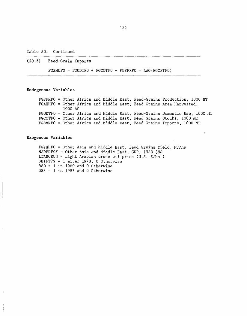
125
Table 20. Continued
(20,5) Feed-Grain Imports
FGSMNFO = FGUDTFO + FGCOTFO - FGSPRFO LAG(FGCPTFO)
Endogenous Variables
FGSPRFO Other Africa and Middle East, Feed-Grains Production, 1000 MT FGAHHFO Other Africa and Middle East, Feed-Grains Area Harvested,
1000 AC FGUDTFO Other Africa and Middle East, Feed-Grains Domestic Use, 1000 MT FGCOTFO Other Africa and Middle East, Feed-Grains Stocks, 1000 MT FGSMNFO Other Africa and Middle East, Feed-Grains Imports, 1000 MT
Exogenous Variables
FGYHHFO =Other Asia and Middle East, Feed Grains Yield, MT/ha NARPDFOF = Other Asia and Middle East, GDP, 1980 $US LTARCRUD = Light Arabian crude oil price (U.S. $/bbl) SHIFT79 = 1 after 1978, 0 Otherwise D80 1 in 1980 and 0 Otherwise D83 = 1 in 1983 and 0 Otherwise

126
Table 21. Structural parameter estimates of the "other Latin America" feed-grains submodel
(21.1) Feed-Grain Production
(21. 2)
(21.3)
(21.4)
FGSPRNO = 1756.370 + 0,589 LAG(FGSPRNO) (3.36) (5.98)
+ 1179.560 LAG(CORPF) (4.95)
- 548,130 LAG(WHEPF) (3. 45)
[0.37] [ -0. 22]
- 820.788 D76 + 436.605 D79 (3.66) (1.95)
DW = 1.47
Feed-Grain Stocks
FGCOTNO = 717.277 + 0.184 LAG(FGCOTNO) (3.86) (2.15)
+ 0.181 FGSPRNO (5.37) [1.95]
+ 537,875 D80- 191.124 D85 + 322.949 (D77 + D81) (6.99) (2.27) (5.62)
R2 = 0.94 DW = 2.02
Feed-Grain Imports
FGSMNNO = -1463.100 + ( 4. 70)
24.455 NARPDNO -(8.08) [ 2. 02]
6728.830(CORPF/SOMPM) (0.51)
[-0.07]
+ 821.078(D80 + D81 + D82 + D83) - 554.892 LAG(CORPF) (6.09) (2.24)
+ 379,717 LAG(WHEPF) (2.58) [0. 72]
DW = 1.87
Feed-Grain Domestic Use
[-0.80]
FGUDTNO = FGSPRNO + LAG(FGCOTNO) + FGSMNNO - FGCOTNO
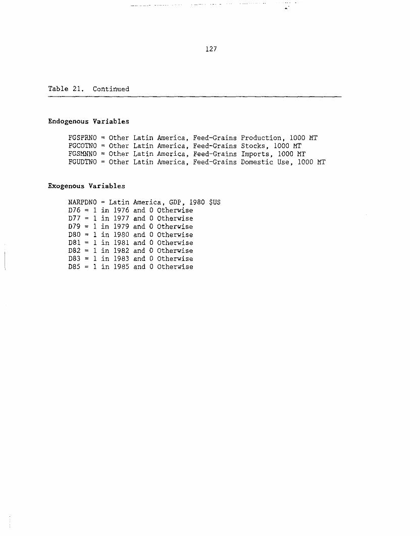
Table 21. Continued
Endogenous Variables
FGSPRNO = Other FGCOTNO = Other FGSMNNO = Other FGUDTNO Other
Exogenous Variables
NARPDNO = Latin D76 = 1 in 1976 D77 1 in 1977 D79 = 1 in 1979 D80 = 1 in 1980 D81 1 in 1981 D82 = 1 in 1982 D83 = 1 in 1983 D85 1 in 1985
127
Latin America, Feed-Grains Latin America, Feed-Grains Latin America, Feed-Grains Latin America, Feed-Grains
America, GDP, 1980 $US and 0 Otherwise and 0 Otherwise and 0 Otherwise and 0 Otherwise and 0 Otherwise and 0 Otherwise and 0 Otherwise and 0 Otherwise
Production, 1000 MT Stocks, 1000 MT Imports, 1000 MT Domestic Use, 1000 MT

128
grain production, lagged stocks, and dummy variables. Feed-grain imports (21.3)
are estimated as a function of income, U.S. corn price, U.S. wheat price, and
U.S. soybean meal price. Feed-grain domestic use is derived as a residual in
equation (21.4).
Rest-of-the-World Submodel
For the rest of the world (ROW), feed grains (corn, barley, and oats) and
sorghum are modeled separately in the feed-grains submodel, illustrated in Table
22. Feed-grain area harvested (22.1) is estimated as a function of corn price,
wheat price, lagged acreage, and dummy variables. Own-price supply elasticity
is 0.16 and cross-price elasticity is -0.16 •. Feed-grain production (22.2) is
described as area times yield. Explanatory variables in the domestic use
equation (22.3) are barley price, wheat price, income, and dummy variables.
Feed-grain stocks (22.4) are estimated as a function of production, barley
price, lagged stocks, and dummy variables. Feed-grain imports (22.5) are
defined as domestic demand minus domestic supply.
The structure of the sorghum model is similar to that of the feed-grains
model. Sorghum area harvested (22.6) is estimated as a function of sorghum
price, lagged acreage, and a set of dummy variables. Estimated own-price supply
elasticity is 0.15. Sorghum production (22.7) is defined as area times yield.
Explanatory variables in the domestic use equation (22.8) are sorghum price,
corn price, soybean meal price, production, income, and dummy variables.
Own-price demand elasticity is -0.27, and cross-price elasticities are 0.37
(corn price) and 0.02 (soybean-meal price). Sorghum stocks (22.9) are estimated
as a function of production, lagged stocks, and dummy variables. Sorghum
imports (22.10) are described as domestic demand minus domestic supply.

129
Table 22. Structural parameter estimates of the ROW feed-grains submodel
(22.1) Feed-Grain Area Harvested
(22. 2)
(22.3)
(22.4)
FGAHHROW = 361.005 + 0.873 LAG(FGAHHROW) (2.18) (9.73)
+ 1.514 LAG(CORPF * NIMERUUS) (2.39) [0.16]
+ 127.641(079 + 081)
OW= 1.91
Feed-Grain Production
FGSPRROW = FGAHHROW * FGYHHROW
Feed-Grain Domestic Use
- 1.238 LAG(WHEPF * NIMERUUS) (2.57)
[-0.16]
FGUOTROW = 4514.460 - 21.985 BARPF * NIMERUUS + 17.422 RERGOPFG (3.15) (2.88) (2.84)
[-0.48] [0.68]
+ 6.847 WHEPF ( l. 50)
* NIMERUUS + 3693.470 OAT6977 (10.64)
[ 0. 22]
- 1963.060(071 + 072) (3.47)
OW= 2.95
Feed-Grain Stocks
FGCOTROW = 1614.650 + 0.400 LAG(FGCOTROW) + 0.333 FGSPRROW
R2 = 0.98
(2.02) (4.97) (3.60)
- 3.361 ( l. 29)
[-0.23]
[0.98]
BARPF * NIMERUUS- 3415.710 SHIFT74 (6.60)
OW= 2.39

130
Table 22. Continued
(22.5) Feed-Grain Imports
(22.6)
(22. 7)
(22.8)
FGSMNROW = FGUDTROW + FGCOTROW - FGSPRROW - LAG(FGCOTROW)
Sorghum Area Harvested
SGAHHROW = 2696.380 + 0.652 LAG(SGAHHROW) (1.96) (7.18)
+ 100323.000 LAG(SORPF/NARDDU9) + 2851.820 D85 (3.63) (4.68) [ 0. 15]
- 2987.720 D76 + 1651.370 D73 (4.73) (2.80)
+ 1950.950(D67 + D69 + D70 + D71) (4.88)
DW = 2.32
Sorghum Production
SGSPRROW = SGAHHROW * SGYHHROW
Sorghum Domestic Use
SGUDTROW = 2341.870 + 0.787 SGRGDPRE + 0.733 SGSPRROW
R2 = 0.97
(0.57) (2.33) (6.31)
- 275076.000 SORPF/NARDDU9 ( 1. 90)
[-0.27]
+ 308263,000 CORPF/NARDDU9 (2.39) [0.34]
+ 227.612 SOMPM/NARDDU9 - 1502.510(D77 + D78 + D79) (0.91) (3.55) [0. 02]
+ 2859.320 D81 - 3131.590 D85 (4.30) (3.22)
DW = 2.48
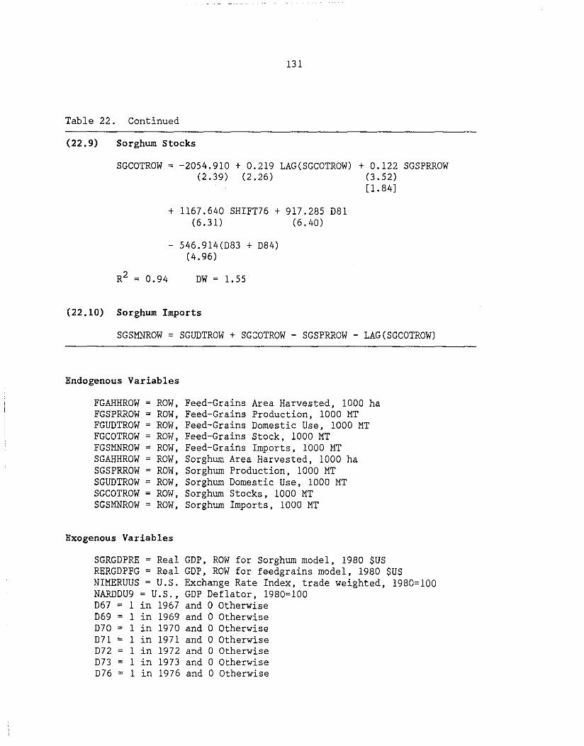
131
Table 22. Continued
(22.9) Sorghum Stocks
SGCOTROW ~ -2054.910 + 0.219 LAG(SGCOTROW) (2.39) (2.26)
R2 ~ 0.94
+ 1167.640 SHIFT76 + 917.285 D81 (6.31) (6.40)
- 546.914(D83 + D84) (4.96)
DW ~ 1.55
(22.10) Sorghum Imports
+ 0.122 SGSPRROW (3.52) [ l. 84]
SGSMNROW ~ SGUDTROW + SGCOTROW - SGSPRROW - LAG(SGCOTROW)
Endogenous Variables
FGAHHROW FGSPRROW FGUDTROW FGCOTROW ~ FGSMNROW ~ SGAHHROW ~
SGSPRROW ~ SGUDTROW ~ SGCOTROW ~ SGSMNROW ~
ROW, Feed-Grains Area Harvested, 1000 ha ROW, Feed-Grains Production, 1000 MT ROW, Feed-Grains Domestic Use, 1000 MT ROW, Feed-Grains Stock, 1000 MT ROW, Feed-Grains Imports, 1000 MT ROW, Sorghum Area Harvested, 1000 ha ROW, Sorghum Production, 1000 MT ROW, Sorghum Domestic Use, 1000 MT ROW, Sorghum Stocks, 1000 MT ROW, Sorghum Imports, 1000 MT
Exogenous Variables
SGRGDPRE Real GDP, ROW for Sorghum model, 1980 $US RERGDPFG ~ Real GDP, ROW for feedgrains model, 1980 $US NIMERUUS ~U.S. Exchange Rate Index, trade weighted, 1980~100 NARDDU9 ~U.S., GDP Deflator, 1980~100
D67 ~ 1 in 1967 and 0 Otherwise D69 1 in 1969 and 0 Otherwise D70 1 in 1970 and 0 Otherwise D71 ~ 1 in 1971 and 0 Otherwise D72 1 in 1972 and 0 Otherwise D73 1 in 1973 and 0 Otherwise D76 1 in 1976 and 0 Otherwise

132
Table 22. Continued
D77 l in 1977 and 0 Otherwise D78 = 1 in 1978 and 0 Otherwise D79 1 in 1979 and 0 Otherwise D81 = 1 in 1981 and 0 Otherwise D83 1 in 1983 and 0 Otherwise D84 = 1 in 1984 and 0 Otherwise D85 = 1 in 1985 and 0 Otherwise DAT6977 1 from 69-77, 0 Otherwise SHIFT74 = 1 after 1973, 0 Otherwise SHIFT76 1 after 1975, 0 Otherwise

133
Evaluation
The estimated model presented in the previous section seems to reflect
adequately the structure of the world feed-grains market. The explanatory power
of the model has not been fully investigated, however. This section reviews
several measures of the model's explanatory power. Performance of the model can
be measured in terms of the validity of its estimates, its ability to reproduce
actual data in a dynamic simulation, and its stability.
To measure this model's forecasting ability, a simulation of the model is
run over the sample period (1972-1982). Simulation results are then compared
with actual data. Statistics measuring the model's fitting performance include
mean error (ME) , mean percentage error (MPE) , mean absolute error (MAE) , root
mean square error (RMSE), and root mean square percentage error (RMSPE).
Mean error measures the average error of simulated values from actual
values. The size of the ME depends upon the variable size. To eliminate this
problem, MPE is often used. In computing ME and MPE, positive and negative
deviations offset each other, which might result in small values of error
measurement. To avoid this problem, MAE is used in computing the simulation
statistics.
The RMSE is the square root of the average error of simulated values from
actual values. The size of RMSE depends upon the variable size. To eliminate
this problem, RMSPE is used instead.
The Appendix presents several key simulation statistics for important
endogenous variables. Simulation statistics must always be interpreted
with care. For example, small absolute simulation errors in a variable that
takes a value near zero in some year results in a large RMSPE. Moreover, the
simulation statistics for a particular variable may be unsatisfactory, not

134
because of a particular problem with the equation determining that variable but
because of a problem elsewhere in the model.
In general, the simulation statistics indicate that the model behaves
satisfactorily. Considering the inelasticity of most of the markets represented
in the model, it is not surprising that the poorest results were obtained for
prices and variables very sensitive to absolute and relative prices. For
example, expected nonparticipant net returns are very sensitive to prices, and
participation rates are very sensitive to the relationship between participant
and nonparticipant net returns. The participation rate determines program area
planted and idled, and both nonpacticipant returns and program acreage have an
important effect on nonprogram acreage. Because the RMSPE's for market prices
are generally high, so are those for expected nonparticipant net returns, the
participation rate, program planted and idled area, and nonparticipant area
planted.
The free-stocks equations behave less satisfactorily than most of the other
equations in the model. Stocks are more price-sensitive than most other supply
and demand categories, and thus errors in simulated prices account for part of
the problem. Free stocks are also· more variable than most of the other inputs.
On the other hand, most of the statistics are encouraging for the major
components of supply and demand. The RMSPE is less than 10 percent for most
total area planted and production variables.
The simulation results represent one common approach to model validation.
If a model is to be used for projections and forward-looking policy analysis, it
is not sufficient to evaluate the ability of the model to replicate historical
data. It is also necessary to assess the ability of the model to provide
defensible answers to the questions it is intended to address. An examination
135
of model elasticities is one way of assessing the plausibility of the model's
behavior. The third section reported single-equation elasticities evaluated at
the means of all variables. Because of the model's many interactions, how the
model behaves when all equations are operating simultaneously should be
considered. Tables 23-25 provide model-elasticity estimates obtained by
shocking a particular variable and allowing the effects to feed through all
equations in the model. These elasticities are evaluated in the 1982/83 crop
year.
The U.S. production elasticities reported in Table 23 represent the net
effect of all model equations directly or indirectly affecting planted area. In
general, the results are consistent with expectations. Own-price elasticities
are positive and cross-price elasticities are negative for all crops. The
production elasticities reported in Table 23 for both the United States and
other countries are inelastic with respect to own prices.
Domestic demand elasticities are reported in Table 24. All own-price
elasticities are negative, which is consistent with expectations. Substitute
crop prices have a positive effect on domestic demand components. Price
transmission elasticities are given in Table 25. The price-transmission
elasticities for Canada, Australia, Thailand, South Africa, and Japan are
close to one because of their free-trade policies in feed grains. The price
transmission elasticities for Argentina, Brazil, and Mexico are well below one
because of their restrictive trade policies in feed grains.
Uses of the Model
This section discusses the broader applicability of the model and briefly
identifies some of the reports and publications prepared by utilizing the model.
Included also is a general description of the experience in running the model.

136
Table 23. Summary of estimated production elasticities from the feed-grains trade model
----------------------Elasticity with Respect to------------------------Country/ Corn Sorghum Barley Oats Wheat Soybean Rapeseed Wool
Region Price Price Price Price Price Price Price Price
u.s. a Corn 0.08 -0.02 Sorghum 0.27 -0.04 Barley 0.53 -0.32 -0.33 Oats -0.25 -0.31 1. 05 -0.21
Canada Barley 0.47 -0.03 Corn 0.08 -0.09
Australia Barley 0.35 -0.27 -0.14 Sorghum 0.16 -0.14 -0.12
Argentina Corn 0.39 -0.22 Sorghum -1.19
EC-12 ---Barley Corn 0.07
Thailand Corn 0.02 -0.11
s. Africa Corn 0.04 Sorghum 0.42 -0.21
Japan Barley
Brazil Feed grains 0.19 -0.22 -0.01
Mexico Feed grains 0.05 Sorghum 0.16 -0.25
~ Corn 0.07 -0.04
India Sorghum 0.07 -0.17
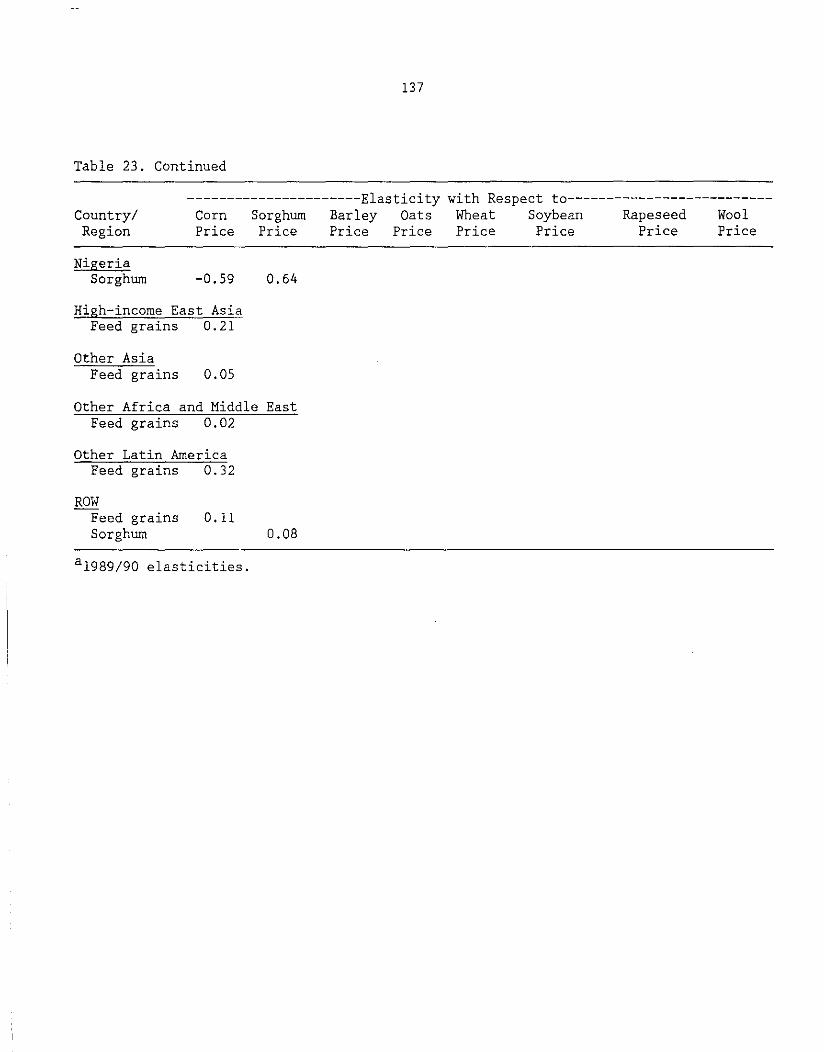
137
Table 23. Continued
----------------------Elasticity with Respect to--------------------------Country/
Region Corn Sorghum Barley Oats Wheat Soybean Rapeseed Wool Price Price Price Price Price Price Price Price
Nigeria Sorghum -0.59
High-income East Asia Feed grains 0.21
Other Asia Feed grains 0.05
0.64
Other Africa and Middle East Feed grains 0.02
Other Latin America Feed grains 0.32
ROW Feed grains Sorghum
0.11
a1989/90 elasticities.
0.08

138
Table 24. Summary of estimated domestic demand elasticities from the feed-grains trade model
Country/ Region
u.s. Corn food Corn feed Corn stocks Sorghum non-
feed Sorghum feed Sorghum stocks Barley nonfeed Barley feed Barley stocks Oats nonfeed Oats feed use Oats stocks
Canada Barley use Corn use
Australia Barley use Barley stocks
Argentina Corn use Corn stocks Sorghum use Sorghum stocks
EC-12 Corn use Corn stocks Barley feed Barley food
Thailand Corn feed use Corn stocks
South Africa Corn use Corn stocks Sorghum use Sorghum stocks
USSR Total feed-grain use
China Total feed-grain use
--------------------Elasticity with Respect to--------------------Corn Sorghum Barley Oats Price Price Price Price
Soy Meal Wheat Price Price Income
-0.14 0.09 1.59 -0.29 0.06 -1.64
0.48 -1.42 o. 71 1.21 -2.08 0.47
-1.51 -0.02 0.31
0.43 -0.66 0.06 0.48
-0.04 -0.95 0.27 -0.52
-0.35
-0.09 0.08 -0.24 0.14 o. 10 0.82
-0.81 0.37 0.40 -5.21
-0.25 0,28 -1.00
2.58 -3.62 -1.71
-0.58 0.06 0.41 0.19 -0.35
-0.15 0.30 -0. 13 0.78
-0.11 0.88 -0.35
-0.34 0.37 -0.53
-0.13 0.85 -0.35
-0.03
0,01

139
Table 24. Continued
--------------------Elasticity with Respect to--------------------Country/
Region Corn Sorghum Barley Oats Price Price Price Price
Soy Meal Wheat Price Price Income
E. Euro12e Total feed grains 0.16
Japan Corn use -0.04 0.30 Corn stocks -0.14 Sorghum use 0.52 -0.51 0.51 Barley use 0.42
Brazil Feed-grain use -0.08 0.61
Mexico Sorghum use -0.43 0.94 Feed-grain use -0.31 0.28 0.41
~ Corn use 0.48 Corn stocks -0.45
Saudi Arabia Barley use 0.30
Nigeria Sorghum use -0.002
HIEAa Feed-grain use -0.02 1. OS Feed-grain
stock -0.03
Other Asia Feed-grain use -0.01 0.22
Other Africa and Middle East Feed-grain
stocks -0.03 0.17
Other Latin America Feed-grain
imports -0.02 0.02 1.32
ROWb Feed-grain use -0.58 0.23 0.84 Feed-grain stocks -0.52
Rowb Sorghum use 0.22 -0.18 0.02 0.29
~High-income East Asia. ROW category includes different countries for feed-grains and sorghum demand, respectively.

140
Table 25. Key price-transmission elasticities of feed-grains prices with respect to U.S. feed-grains prices
Country/ Region u.s. Corn Price u.s. Barley Price u.s. Sorghum Price
Canada Barley 1. 04 Corn 0.94
Australia Barley 1. 01 Sorghum 1.02
Argentina Corn 0.64 Sorghum 0.49
Thailand Corn 0.99
South Africa Corn 1. 05 Sorghum 0.95
Japan Corn 0.83
Brazil Corn 0.53
Mexico Corn 0.16 Sorghum 0.39
fuiTE! Corn 0.86

141
As indicated in previous sections, FAPRI models are highly flexible: they
function in a highly interactive environment but are also capable of being
operated independently. SAS and AREMOS, an econometric package developed by The
WEFA Group, are generally used for estimation. The policy analyses, however,
are conducted on microcomputers using LOTUS 1-2-3. One of the major advantages
of using LOTUS 1-2-3 for policy analyses is that this program provides an
opportunity for the analyst to examine changes occurring in endogenous variables
during iteration.
The feed-grains trade model, along with other trade models and domestic
crops and livestock models, is used on a regular basis to generate 10-year
projections of demand, supply, trade, prices, and other key agricultural
variables in the United States and other countries. These projections serve as
a baseline scenario for policy-impact analyses. The models were used to analyze
farm bill options during debate in 1985 and 1990, as well as some cost-cutting
alternatives that were proposed later in response to budget pressure. Scenarios
were also evaluated on specific trade and policy issues. A selected list of
publications from these studies follows:
• "Impacts of EEC Policies on U.S. Export Performance in the 1980s." W. H. Meyers, R. Thamadoran, and M. Helmar. Chapter 6 in Confrontation or Negotiation: United States Policy and European Agriculture. New York: Associated Faculty Press, 1985.
• "Macroeconomic Impacts on the U.S. Agricultural Sector: A Quantitative Analysis for 1980-84." W. H. Meyers, M. Helmar, S. Devadoss, and D. Blanford. Chapter 24 in Embargoes, Surplus Disposal, and U.S. Agriculture AER Number 564, ERS/USDA, December 1986.
• "An Export Disposal Policy for Wheat and Corn Stocks by the United States: A Quantitative Analysis for 1977-1984." W. H. Meyers, S. Devadoss, and M. Helmar. Chapter 19 in Embargoes, Surplus disposal, and U.S. Agriculture, AER Number 564, ERS/USDA, December 1986.

142
• "The Iowa State University FAPRI Trade Model." W. H. Meyers, S. Devadoss, and M. Helmar. Proceedings of the International Agricultural Trade Research Consortium on Agricultural Trade Modeling: The State of Practice and Research Issues, Staff Report No. AGES861215, IED/ERS/USDA, June 1987, pp. 44-56.
• "Agricultural Trade Liberalizations: Cross-Commodity and Cross-Country Impact Products." W. H. Meyers, S. Devadoss, and M. Helmar. Journal of Policy Modeling, Vol. 9, No. 3 (November 1987), pp. 455-482.
• "FAPRI Ten-Year International Agricultural Outlook, July 1987." Food and Agricultural Policy Research Institute. Staff Report #4-87. University of Missouri -Columbia ancj. Iowa State University, Ames.
• "FAPRI Ten-Year International Agricultural Outlook, March 1988." Food and Agricultural Policy Research Institute. Staff Report #1-88, University of Missouri-Columbia and Iowa State University.
• "Commodity Market Outlook and Trade Implications Indicated by the FAPRI Analysis." W. H. Meyers, S. Devadoss, and B. Angel. Food Aid Projections for the Decade of the 1990s. Report of an ad hoc panel meeting, National Research Council, October 6-7, 1988, pp. 98-121.
• "Agricultural Market Outlook and Sensitivity to Macroeconomic, Productivity, and Policy Changes." S. R. Johnson, W. H. Meyers, P. Westhoff, and A. Womack. CARD Working Paper #87-WP36 (November 1988). Center for Agricultural and Rural Development, Iowa State University, Ames.
• "Policy Scenarios with the FAPRI Commodity Models." CARD Working Paper #88-WP41 (December 1988). Center for Agricultural and Rural Development, Iowa State University, Ames.
• "FAPRI U.S. and World Agricultural Outlook, May 1989." Food and Agricultural Policy Research Institute. Staff Report #2-89. University of Missouri-Columbia and Iowa State University.
• "The Impact of the U.S. Export Enhancement Program on the World Wheat Market." H. G. Brooks, S. Devadoss, and W. H. Meyers. CARD Working Paper #89-WP46 (December 1989). Center for Agricultural and Rural Development, Iowa State University, Ames.
The feed-grains trade model should be evaluated as a model under
construction. The model is continually being revised to deal with perceived
problems, so this documentation must be seen as a snapshot of a work in
progress, rather than as a portrait of a completed effort. Some of the

143
shortcomings of the model have been pointed out, and efforts will be made to
correct these shortcomings in the months and years to come.
Any revisions to the model should be made recognizing the strengths of the
model. In its present form, the model makes it possible to examine a variety of
issues important in policy analysis and market outlook. For the most part, the
model behaves in an internally consistent and intuitively appealing way.
Although it may be desirable to impose more structure upon the model and to use
more appropriate estimation techniques, the current strengths of the model
should not be sacrificed unnecessarily in the process.

145
APPENDIX
Simulation Statistics from the Dynamic Simulation of the World Feed-Grains Trade Model
VARIABLE MEAN MEAN % MEAN ABS RMS RMS % ERROR ERROR ERROR ERROR ERROR
COMPRU9F 0.06867 954160995 0. 07143 0.12399 82540.05
COAPNU9F -5.31338 -8.52318 5.41716 9.38806 14.87173 COYHAU9F 0. 07222 0.07229 0.07222 0.13417 0.13422 CONRNU9F -1.87805 -1.53586 22.69363 29.44899 25.75262 CONRPU9F 2.90509 1. 89494 11.69931 16.62321 12.81442 SBNRNU9F -1. 63E-05 -1.21E-05 3.24E-05 3.82E-05 3.22E-05
COAIAU9F 0.78394 22.00762 0.78394 1. 45723 48.62771 COAPPU9F 4.88681 7.60E+10 5.05407 9.06168 6667948 COAPAU9F -0.42656 -0.58747 1.10758 1.22377 1. 60567 COAHAU9F -0.18417 -0.33225 0.81937 1. 05152 1. 58462 COSPRU9F -11.45748 -0.26088 74.50196 93.54089 1. 53303 COUFEU9G -0.29380 -0.46299 1.23264 1. 74515 2.67723 COUOFU9C -.0024717 -0.08931 0.03556 0.04264 1. 69042
COUSDU9 -0.30026 -1.74447 0.67661 0.81939 4.58497
COUGAU9 -0.65433 -1.76745 1.13566 2.42727 6.23833 COFREU9 -22.35752 -0.06168 75.06295 98.26025 14.88671 COUOFU9 -0.56272 -0.08930 7.86926 9.44385 1. 69042 COUFOU9 -1.51731 -0.20728 7.30551 8.86246 1.53225 COUFEU9 -16.76152 -0.46299 74.84488 105.51 2.67723 COCOTU9 -22.35752 -0.77982 75.06295 98.26025 8.66177 FGUXNU9 219.27 0.86071 2605.89 3185.52 7.17457 COUXNU9 115.97 0.70534 2720.41 3354.49 7.61831 COUXTU9 4.56533 0.70236 107.10 132.06 7.60844 SGMPRU9 -.0070639 1.43E+09 0.05451 0.09093 92664.38 SGAPNU9 0.31083 8.33908 0.96927 1. 32914 22.33890 SGYHAU9 3.58E-05 6.59E-05 3.58E-05 3.5BE-05 6.64E-05 SGABPU9 .00934446 1. 20743 0.01807 0.02281 2.86235 SGNRNU9 3.74875 8. 72634 9.87446 13.49439 25.62470 SGNRPU9 2.47369 3.56787 4.38849 6.96467 9.04932 WHNRNU9 -8.98E-06 -1.63E-05 9. 71E-06 l.12E-05 l. 94E-05 SGAIAU9 -0.05239 -1.36906 0.09480 0.17088 11.42441 SGAPAU9 0.28710 l. 78141 0.38312 0.53117 3.28135 SGAPPU9 -0.02373 2.03E+10 0.74629 1.14988 1229451 SGAHAU9 0. 39571 3.02233 0.50080 0.68873 5.17008 SGSPRU9 23.67641 3.02240 29.07012 41.4 7677 5.17012 SGUFEU9 4.35103 l. 66063 27.05872 31.00093 6.54194 SGUFOU9 0.35613 3.68982 0.78870 0.99707 9.47213 SGF9LU9 19.45855 -4.06468 48.53070 58.72155 103.93 SGCOTU9 19.45855 11.05919 48.53070 58.72155 51.20989 SGUXNU9 203.09 3.64602 953.10 1089.70 18.03922 SGUXTU9 7.99515 3.64602 37.52148 42.89921 18.03922 BAMPRU9 0.03326. 1.50E+09 0.08463 0.12934 157258 BAAPNU9 0.09624 4.85722 0.75973 0.90652 27.42340 BAABPU9 .00379184 0.42234 . 00950811 0.01143 1.24591 BAYHAU9 .00015633 .00033759 .00015633 .00015637 .00033976 BANRNU9 -0.75320 -2.26921 4. 70115 5.93577 l3. 69429 BANRPU9 0.55400 0.92642 1.83324 2.99033 4.34015 OANRNU9 -1.76658 -8.42785 6.18771 7.26652 26.04502 BAAIAU9 -0.04400 5.86364 0.17140 0.35491 21.87889

146
VARIABLE MEAN MEAN % MEAN ABS RMS RMS % ERROR ERROR ERROR ERROR ERROR
BAAPAU9 0.34562 3.98160 0.44560 0.61027 6. 91151 BAAPPU9 0.24937 l. 30E+l0 0. 72619 l. 04515 1368144
BAAHAU9 0.35370 4.40200 0.41305 0.57008 7.01706 BASPRU9 17.67088 4.40235 20.24538 28.89350 7.01728 BAUFEU9 12.08818 5.96489 14.27238 18.78033 9.57326 BAUFOU9C .00053626 0.09433 . 00777799 .00889251 1.24202 BAF9LU9 11.34467 9.00888 16.09727 22.04687 17.57032 BACOTU9 11.34467 7.52149 16.09727 22.04687 15.32927 BAUFOU9 0.10110 0.09433 1. 71159 l. 95750 1.24202 BAUXTU9 4.72558 17.17393 14.71380 19.18843 45.31030 OAMPRU9 -.0015233 -1.44025 .00152334 .00505235 4.77677 OAAHAU9 0.13463 1.34766 0.85564 1.01717 8.91682 OAAPAU9 0.14222 1.17258 0.95383 1.14155 7.03588 OAYHAU9 -3.25E-05 -6.38E-05 3.25E-05 3.36E-05 6.66E-05 CONRNU9 l. 77927 1.37236 19.03631 26.83481 23.87806 OANRPU9 -l. 82299 -8.02309 6.04353 7.04618 25.68062 SBNRNU9 -2.01E-05 -1. 59E-05 2.86E-05 3.60E-05 2. 97E-05 0AAIAU9 -.0014403 -1.44025 .00144025 .00477678 4. 77678 OAAPNU9 0.15663 l. 34653 0.96823 1.15838 7.27867 0AAPPU9 -0.01440 -1.44025 0. 01440 0. 04777 4.77678 0ASPRU9 6.24534 1.34759 43.81247 51.84205 8.91680 OAUFEU9 8.68326 l. 59375 20.00501 26.49280 5.31576 OAUFOU9C .00022575 0.35206 0. 01312 0.01538 4.42132 OAF9LU9 4.94010 1.96257 25.21033 28.41485 12.68252 OASMNU9 -0.03043 -43.18576 2.80223 3.82063 203.30 OACOTU9 4.94010 0.90833 25.21033 28.41485 10.87849 OAUFOU9 0.08280 0.35206 2.94411 3.49482 4.42132 OASMTU9 -0.03043 6. 71E+l0 2.80223 3.82063 7245168 COPFMARR 2.60463 1.33967 26.89206 33.88797 12.67511 SGPFMARR 1.58486 0.86221 17.85582 20.99320 9.15835 SBPFMARR 8.62716 2.13411 29.16210 42.70288 6.94543 WHPFMARR -3.60777 -0.64704 13.28491 20.95538 5.73200 CECOTAR -0.36764 -0.62070 0.79019 1.01107 l. 71587 COAHHAR 6.78389 0.66000 158.32 227.60 7.19844 COCOTAR -5.23322 11.11052 104.54 128.45 49.86941 COSMNAR 23.01655 1.17513 356.01 637.69 7.84916 COSPRAR -6.40698 0.66176 517.70 800.80 7.19646 COUDTAR -5.99364 0.04051 12 5. 95 151.52 4.22386 SGAHHAR 115.21 5.68759 179.96 219.10 10.29441 SGCOTAR -0.08290 18.77862 24.74097 32.50462 54.34872 SGSMNAR -349.30 7.87368 556.52 686.11 17.19490 SGSPRAR 322.87 5.68670 517.81 642.48 10.29027 SGUDTAR -27.51077 1.06413 334.45 392.92 17.32652 FGSMNAR 23.01655 l. 07951 356.01 637.69 7.66783 BAPFMAU -424.49 -2.71539 729.55 1012.96 8.47224 SGPFMAU -49.94925 -0.03448 879.28 1193.12 10.54409 SHCOTAU 9.94786 7.08375 10.26327 11.40448 8.03038 GWPFMAU -3.45547 -1.41075 6.34242 10.02437 4.16832 WHPEXAU -3.70343 -3.27889 7.42658 9.31788 8.29839 WHPFMAU -246.62 -2.93823 721.25 895.32 9.48168 BAAHHAU -25.82487 0.44170 317.41 347.84 15.35284

14 7
VARIABLE MEAN MEAN % MEAN ABS RMS RMS % ERROR ERROR ERROR ERROR ERROR
BACOT AU 24.44326 35.06320 49.84557 61.42801 71.96216
BASMNAU 20.14492 l. 59662 444.22 519.42 43.07005 BASPRAU -18.28322 0.43864 379.33 424.00 15.35142 BAUDTAU -6.43738 -0.33170 148.59 175.84 14.50796 SGA!!HAU 53.14331 9.47890 54.19797 62.88104 10.88122 SGCOTAU 3.70495 24.39559 18.52019 23.07295 57.61360 SGSMNAU -148.35 29.91202 148.35 167.51 40.43437 SGSPRAU 99.38588 9.47890 100.93 117.48 10.88121 SGUDTAU -51.60305 -11.31733 70.45686 87.66370 33.39873 FGSMNAU 139.42 -3.05921 563.50 668.73 42.66939 BAPOBCA 0.13919 0.54735 6.26217 7. 92956 8. 77397 COPFMCA -2.81771 -2.15721 11.87021 14.75276 13.10470 RSPM1CA 0.04871 -0.35294 11.57364 13.42926 4.62647 SBPFMCA 0.35549 0.36192 6.08269 7.16184 3.51171 SMPFMCA l. 27795 0.84454 11.50196 17.21827 7.44672 LVCACCA -0.02066 -0.08370 0.25011 0.32865 l. 69367 BAAHHCA -366.41 -7.43133 435.71 535.21 10.99792 BASMNCA 891.60 -25.30289 1068.63 1210.00 35.59047 BASPRCA -822.25 -7.43129 990.12 1210.85 11.00054 BAUDTCA 69.34676 l. 06186 257.90 285.38 4.08436 COAHHCA 3.55234 1.12617 22.72131 26.88015 4.07096 COCOTCA -9.56355 3.57175 59.29414 80.13329 13.73385 COSMNCA 29.37212 92.36064 260.95 334.11 212.07 COSPRCA 10.32121 1.12483 123.84 143.91 4.07227 COUDTCA 46.94623 l. 40351 352.33 403.78 7.53465 FGSMNCA 920.97 -37.39976 1130. 90 1227.26 56.43200 COPFMTH -71.73199 -2.04701 201.01 264.60 16.42253 SGPFMTH -58.59605 -2.00697 171.04 232.48 13.77628 PLSPRTH 6.58826 8.02403 13.84751 16.44615 18.25611 COAHHTH 0.96853 0.10968 23.78098 29.50723 2.13320 COCOTTH 12.48812 41.24080 35.69294 46.73291 113. 96 COSMNTH -3.06458 0. 30431 74.43764 84.23098 4.73026 COSPRTH 7. 67071 0.11386 48.14346 61.40497 2.13132 COUFETH 9.83195 0.26685 48.63586 58.84256 27.61262 FGSMNTH -3.06458 0.30431 74.43764 84.23098 4.73026 SMPFMEO -1.69140 -0.60390 7.23421 9.37054 5.33908 POSPRE2 84.65281 0.97707 185.17 257.55 2.75616 PYSPRE2 7.02067 0.24773 95.43399 113. 98 2.51521 BAAHHE2 -45.78286 -0.37000 62.19146 75.26013 0.60754 BACOTE2 -59.42174 -0.28830 294.37 432.96 l3. 22900 BASMNE2 129.66 -10.03809 554.13 759.40 138.67 BASPRE2 -154.23 -0.37000 210.78 253.43 0.60754 BAUFEE2 60.05552 0.20640 458.53 559.87 l. 70568 BAUHTE2 -54.76520 -0.57528 196.47 224.00 2. 27752 COAHHE2 42.15126 1.12887 66.27192 83.54807 2. 21188 COCOTE2 9.23924 0.31244 199.19 253.61 6.89861 COSMNE2 -247.37 -1.64972 742.35 917.93 4.76636 COSPRE2 184.02 1.12887 311.41 382.73 2.21188 COUDTE2 -86.47077 -0.19969 871.39 1013.55 2.71480 FGSMNE2 -117.72 -1.59481 1113.03 1464.77 7.58780

148
VARIABLE MEAN MEAN % MEAN ABS RMS RMS % ERROR ERROR ERROR ERROR ERROR
COPFMZA 0.05098 3.58590 16.11529 19.49860 19.24701 SGPFMZA -'55.18451 0.12009 72 4. 64 926.53 10.27966 WHPFMZA 190.24 3.27492 836.45 955.12 10.34514
COARHZA 45.16524 1. 02598 89.77749 109.78 2.51424
COCOTZA 29.17369 90.81157 193.05 234.34 318.59 COSMNZA -141.18 72.94877 624.87 723.71 209.51
COSPRZA 59.33890 1.02597 199.97 267.85 2.51423
COUDTZA -122.07 -2.05976 376.72 422.68 6.62516
SGARHZA -1.47730 0.56699 28.45731 34.27667 13.57640 SGSPRZA -8.24531 0.56698 45.28777 52.99357 13.57639 SGUDTZA 1.41498 0.80535 23.65482 30.33212 10.78082 COVIMJP -1178.74 -3.76374 2888.91 3697.18 10.74420 HOCOTJP 0.03356 0. 31994 0.13286 0.15521 l. 83212 PYSPRJP 5.77171 0.26998 17.55612 25.20639 2.46884 BAARHJP -14.10511 -13.93462 19.89812 22.03704 22. 77607· BACOTJP 0.33259 3.74783 77.16546 100.75 21.79072 BASMNJP -22.47168 -1.43244 66.30237 82.69094 6.01666 BASPRJP -44.68392 -13.93462 60.39135 68.31218 22.77608 BAUFEJP -21.92299 -1.50804 50.47059 59.00623 4.70508 BAUHTJP -54.62503 -12.47661 103.49 114.21 23.89764 COCOTJP 0.24677 0.62391 108.67 147.72 12.88077 COSMNJP 168.98 0.93260 512.41 556,62 5.72228 COUDTJP 172. 58 0.88589 473.96 515.43 5.45140 SGCOTJP -65.99527 -12.87387 80.68662 103.84 21.71774 SGSMNJP -81.79503 -0.95404 285.76 357.88 9.18196 SGUDTJP -82.03387 -1.04283 277.88 325.09 8.48398 FGSMNJP 146.51 0.66294 492.03 539.47 4. 71434 CECOTSU 0.06775 0.05239 0.53056 0.62991 0.56746 FGARHSU -1192.64 -2.56960 1692.19 2205.09 4.79826 FGCOTSU 600.69 29.70951 671.03 853.68 57.70396 FGSMNSU 869.61 37.80022 1990.87 2555.17 85.52086 FGSPRSU -1966.77 -2.56960 2837.04 3889.23 4.79826 FGUDTSU -1258.51 -1.51838 3269.60 3531.58 4.21887 HOCOTE8 -0.54917 -0.83040 1.15896 1.39307 2.22625 FGSPRE8 -516.22 -0.98467 761.80 975.20 1. 85660 FGCOTE8 -56.65738 -1.19541 213.90 261.19 10.66911 FGUDTE8 -707.17 -1.20286 1459.72 1646.37 2.94752 FGSMNE8 -232.64 1. 41096 1295.86 1497.74 29.43054 FGAHHE8 -142.42 -0.98467 214.93 264.95 1.85660 HOCOTCN -0.99679 -0.20086 8.12983 9.54447 3.41679 FGARHCN -169.20 -0.76442 336.81 459.65 2. 08013 FGUDTCN -521.51 -1.03281 1037.19 1209.82 2.53285 FGSPRCN -275.44 -0.76442 714.58 903.88 2. 08013 FGSMNCN -244.43 1050.81 809.98 924.53 3118.08 FGAHHR4 8.13678 3.15196 34.93972 41.85965 8.67651 FGCOTR4 -111.67 -1.37005 279.65 319.60 22.41220 FGUDTR4 -96.42578 -1.70712 220.87 276.67 4.93346

149
VARIABLE MEAN MEAN % MEAN ABS RMS RMS % ERROR ERROR ERROR ERROR ERROR
FGSPRR4 26.27451 3.15197 85.49704 104. 7l 8.67652 FGSMNR4 -102.74 -2.50359 224.86 259.53 6.75907 COPFMRBR 292.29 4.15136 813.37 1054.05 16.28529 WHPFMRBR 301.65 2.68680 517.73 671.55 6.05587 SBPFMRBR 851.19 5.94966 1734.37 2604.20 19.41611 FGAHHBR 184.43 l. 80155 638.12 763.54 6.76288 FGUDTBR 219.08 l. 06443 486.42 592.42 3.40010 FGSPRBR 296.25 l. 80155 981.96 1152.43 6.76288 FGSMNBR -77.17444 22.43592 1065.61 1434.82 249.46 COPFMMXR 40.90076 l. 35796 137.57 163.37 4.24797 SGPFMMXR -1135.12 -37.71501 1135.12 12 01.15 38.69064 WHPFMMXR 171.35 4.72296 217.85 279.58 8.48418 POSPRMX -176.87 -22.32433 176.87 191.12 23.36837 FGAH!IMX -60.35520 -0.64541 186.39 205.33 2.58348 FGCOTMX -58.97374 -1.89149 114.12 126.96 31.42600 FGUDTMX -1276.96 -10.07792 1314.68 1761.95 13.85476 FGSPRMX -74.53489 -0.64541 219.54 241.02 2.58347 FGSMNMX -1190.01 -76.30048 1298.07 1764.24 124.40 SGAH!IMX -366.15 -32.71025 380.09 418.13 37.70080 SGCOTMX -140.84 -106.26 159.42 198.38 285.72 SGUDTMX 19.61030 4.46831 432.25 524.32 20.65143 SGSPRMX -1010.00 -32. 7102 5 1037.90 1154.96 37.70080 SGSMNMX 1032.18 226.37 1032.18 1116. 38 323.20 COPFMEG 5.07662 8.03033 10.27258 13.41314 17.50329 COSPREG -6.69008 -0.48215 82.52108 97.09313 3.32049 COCOTEG 75.33648 l.18E+l3 213.63 409.64 l. 24E+09 COUDTEG 136.40 7.95968 225.47 389.36 25.10591 COAH!IEG -2.68619 -0.48274 21.63005 25.46592 3.31804 COSMNEG 151.54 94.31192 260.70 437.25 311.50 FGSMNEG 151.54 94.31191 260.70 437.25 311. 50 EGSPRSA 2.01817 -0.37836 15.52853 22.62711 8. 43879 BAUDTSA -3.86641 -14.09296 234.14 328.24 312.30 BASMNSA -3.86641 -90.06810 234.14 328.24 636.70 FGSMNSA -3.86641 11.59490 234.14 328.24 138.82 SGPFMNG 0. 41599 1. 67139 5.41618 7.01691 8.56454 COPFMNG 0.51871 1.16258 4.85304 6.65848 6.52481 SGAHHNG -28.16769 -0.39456 72.70190 92.79794 1.69217 SGUDTNG -2.85629 -0.04921 56.55966 63.70818 1.74207 SGSPRNG -13.03162 -0.39455 50.19004 66.49798 1. 69218 SGAHHIN -215.25 -1.31587 263.40 313.52 l. 92876 SGCOTIN -23.06123 -3.14143 35.93889 43.53019 6. 55774 SGUDTIN -208.12 -2.02908 254.94 286.24 2.78533 SGSPRIN -145.01 -1.31587 176.73 212.59 l. 92876 FGSPRNO 71.43142 1. 46564 328.34 396.58 6.22965 FGCOTNO 36.04320 16.23362 97.17264 110.91 31.90571 FGSMNNO -116.92 -7.94362 256.09 296.75 17.50903 FGUDTNO -55.83711 -0.58254 201.45 248.46 3.13378 FGSPRFO 396.55 1. 72737 1176.69 1487.44 5.49464 FGCOTFO 0.02511 6.54349 442.86 585.90 23.21762 FGUDTFO 399.61 1. 66028 1207.67 1561.68 5.34979
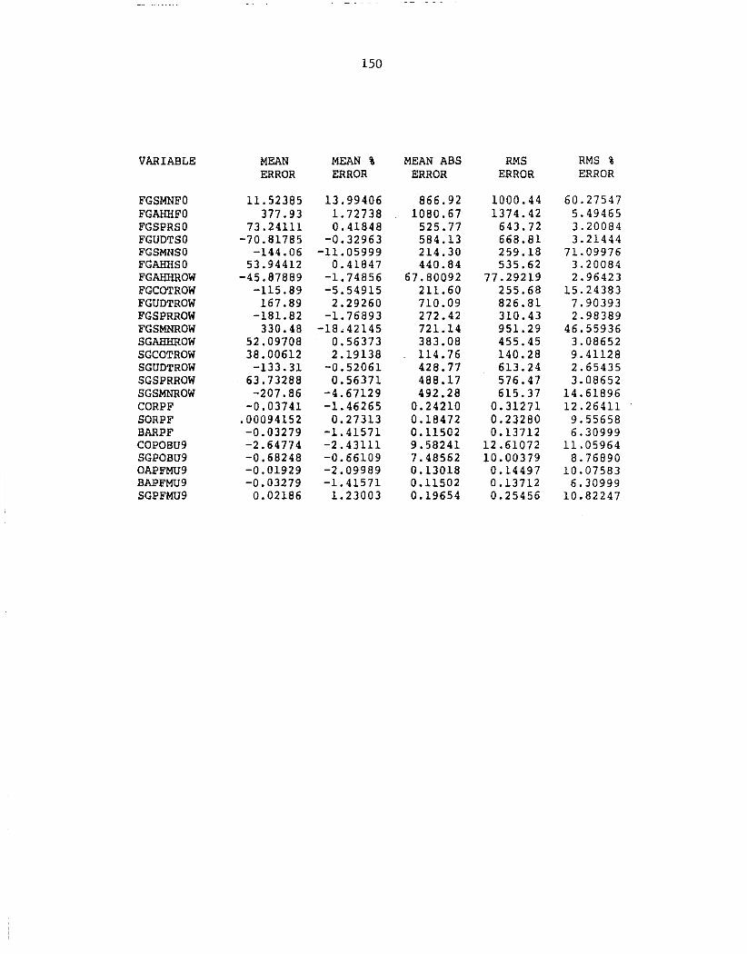
150
VARIABLE MEAN MEAN % MEAN ABS RMS RMS % ERROR ERROR ERROR ERROR ERROR
FGSMNFO 11.52385 l3. 99406 866.92 1000.44 60.27547 FGAHHFO 377.93 1.72738 1080.67 1374.42 5.49465 FGSPRSO 73.24111 0.41848 525.77 643.72 3.20084 FGUDTSO -70.81785 -0.32963 584,13 668.81 3.21444 FGSMNSO -144.06 -11.05999 214.30 259.18 71.09976 FGAHHSO 53.94412 0.41847 440.84 535.62 3.20084 FGAHHROW -45.87889 -l. 74856 67.80092 77.29219 2.96423 FGCOTROW -115.89 -5.54915 211.60 255.68 15.24383 FGUDTROW 167.89 2.29260 710.09 826.81 7.90393 FGSPRROW -181.82 -1.76893 272.42 310.43 2.98389 FGSMNROW 330.48 -18.42145 721.14 951.29 46.55936 SGAHHROW 52.09708 0.56373 383.08 455.45 3.08652 SGCOTROW 38.00612 2.19138 114.76 140.28 9.41128 SGUDTROW -133.31 -0.52061 428.77 613.24 2.65435 SGSPRROW 63.73288 0.56371 488.17 576.47 3.08652 SGSMNROW -207.86 -4.67129 492.28 615.37 14.61896 CORPF -0.03741 -1.46265 0.24210 0.31271 12.26411 SORPF . 00094152 0.27313 0.18472 0.23280 9.55658 BARPF -0.03279 -l. 41571 0.11502 0.13712 6.30999 COPOBU9 -2.64774 -2.43111 9.58241 12.61072 11.05964 SGPOBU9 -0.68248 -0.66109 7.48562 10.00379 8.76890 OAPFMU9 -0.01929 -2.09989 0.13018 0.14497 10.07583 BAPFMU9 -0.03279 -1.41571 0.11502 0 .13712 6.30999 SGPFMU9 0.02186 l. 23003 0.19654 0.25456 10.82247

151
REFERENCES
Bahrenian, Aniss. 1987. "EC Common Agricultural Policy and World Trade in Feed Grains: A Multi-Region, Nonspatial Price Equilibrium Analysis." Unpublished Dissertation, Department of Economics, Iowa State University, Ames.
Burtin, Jacques. 1987. "The Common Agricultural Policy and Its Reform." European Documentation, Office for Official Publications of the European Communities.
Commonwealth Bureau of Census and Statistics. Various years. Yearbook of the Commonwealth of Australia. Canberra, Australia.
de Gorter, Harry, and Brian Paddock. 1985. "The Impact of U.S. Price Support and Acreage Reduction Measures on Crop Output." International Trade Policy Division, Agriculture Canada, November 18. Unpublished manuscript.
FAO. FAO Trade Yearbook. Various years. Rome, Italy.
Food and Agricultural Policy Research Institute. 1987. "FAPRI Ten-Year International Agricultural Outlook." FAPRI Staff Report /f4-87. University of Missouri-Columbia and Iowa State University.
1988. "FAPRI Ten-Year International Agricultural Outlook." FAPRI Staff Report #1-88. University of Missouri-Columbia and Iowa State University.
Houck, J. P., and Mary E. Ryan. 1972. "Supply Analysis States: The Impact of Changing Government Programs." Agricultural Economics 54(May):184-91.
for Corn in the United American Journal of
International Monetary Fund. Various years. International Financial Statistics. Washington, D.C.: International Monetary Fund.
Liu, Karen. 1985. "A Grains, Oilseeds, and Livestock Model of Japan." USDA, ERS, IED.
Meilke, K. D. 1976. "Acreage Response to Policy Variables in the Prairie Provinces." American Journal of Agricultural Economics 58(August):572-77.
Meyers, W. H., M. D. Helmar, and S. Devadoss. 1986. "FAPRI Trade Model for the Soybean Sector: Specification, Estimation, and Validation." Working Paper No. 86-SR2 (Revised). Center for Agricultural and Rural Development, Iowa State University, Ames.
Miller, Geoff. 1987. "The Political Economy of International Agricultural Policy Reform." Australian Government Publishing Service, Canberra.

152
Organization for Economic Cooperation and Development. 1987. "National Policies and Agricultural Trade: Study on the European Economic Community." OECD, Paris.
Sanderson, F. H. 1978. Japan's Food Prospects and Policies. Washington, D.C.: Brookings Institution.
Spriggs, J. 1981. An Econometric Analysis of Canadian Grains and Oilseeds. Technical Bulletin No. 1662. U.S. Department of Agriculture, Economic Research Service.
1978. An Econometric Analysis of Export Supply of Grains in Australia. FAER No, 150. U.S. Department of Agriculture, Economics, Statistics, and Cooperative Service,
Statistics Canada. Various years. Grain Trade of Canada. Ottawa, Canada: Statistics Bureau, Agricultural Branch.
Sullivan, John, John Wainio, and Vernon Roningen. 1989. "A Database for Trade Liberalization Studies." USDA, ERS.
Tyers, Rodney. 1984. "Agricultural Protection and Market Insulation: Analysis of International Impacts by Stochastic Simulation." Australia-Japan Research Centre, Australia National University, Canberra.