The Wild Bootstrap for MultivariateNelson-Aalen Estimators

∗ Tobias Bluhmki, ∗ Dennis Dobler, Jan Beyersmann, Markus PaulyUlm University, Institute of Statistics,

Helmholtzstrasse 20, 89081 Ulm,Germany

February 6, 2017

Abstract

We rigorously extend the widely used wild bootstrap resamplingtechnique to the multivariate Nelson-Aalen estimator under Aalen’smultiplicative intensity model. Aalen’s model covers general Marko-vian multistate models including competing risks subject to indepen-dent left-truncation and right-censoring. This leads to various sta-tistical applications such as asymptotically valid confidence bands ortests for equivalence and proportional hazards. This is exemplified ina data analysis examining the impact of ventilation on the durationof intensive care unit stay. The finite sample properties of the newprocedures are investigated in a simulation study.

Keywords: conditional central limit theorem, counting process, equiva-lence test, proportional hazards, Kolmogorov-Smirnov test, survival analysis,weak convergence.

1 Introduction

One of the most crucial quantities within the analysis of time-to-event datawith independently right-censored and left-truncated survival times is the

∗Authors with equal contribution, e-mail: tobias.bluhmki@uni-ulm.de,dennis.dobler@uni-ulm.de, jan.beyersmann@uni-ulm.de, markus.pauly@uni-ulm.de

1

arX

iv:1

602.

0207

1v2

[st

at.M

E]

3 F

eb 2

017

cumulative hazard function, also known as transition intensity. Most com-monly, it is nonparametrically estimated by the well-known Nelson-Aalen es-timator [Andersen et al., 1993, Chapter IV]. In this context, time-simultaneousconfidence bands are the perhaps best interpretative tool to account for re-lated estimation uncertainties.

The construction of confidence bands is typically based on the asymptoticbehavior of the underlying stochastic processes, more precisely, the (properlystandardized) Nelson-Aalen estimator asymptotically behaves like a Wienerprocess. Early approaches utilized this property to derive confidence bandsfor the cumulative hazard function; see e.g., Bie et al. [1987] or Section IV.1.3in Andersen et al. [1993].

However, Dudek et al. [2008] found that this approach applied to smallsamples can result in considerable deviations from the aimed nominal level.To improve small sample properties, Efron [1979, 1981] suggested a computa-tionally convenient and flexible resampling technique, called bootstrap, wherethe unknown non-Gaussian quantile is approximated via repeated generationof point estimates based on random samples of the original data. For a de-tailed discussion within the standard right-censored survival setup, see alsoAkritas [1986], Lo and Singh [1986], and Horvath and Yandell [1987]. Thesimulation study of Dudek et al. [2008] particularly reports improvementsof bootstrap-based confidence bands for the hazard function as comparedto those using asymptotic quantiles. An alternative is the so-called wildbootstrap firstly proposed in the context of regression analyses [Wu, 1986].As done in Lin et al. [1993], the basic idea is to replace the (standardized)residuals with independent standardized variates – so-called multipliers –while keeping the data fixed. One advantage compared to Efron’s bootstrapis to gain robustness against variance heteroscedasticity [Wu, 1986]. Usingstandard normal multipliers, this resampling procedure has been applied toconstruct time-simultaneous confidence bands for survival curves under theCox proportional hazards model [Lin et al., 1994] and adapted to cumula-tive incidence functions in the more general competing risks setting [Lin,1997]. The latter approach has recently been extended to general wild boot-strap multipliers with mean zero and variance one [Beyersmann et al., 2013],which indicate possible improved small sample performances. This result wasconfirmed in Dobler and Pauly [2014] as well as Dobler et al. [2015], wheremore general resampling schemes are discussed.

In contrast to probability estimation, the present article focuses on thenonparametric estimation of cumulative hazard functions and proposes a

2

general and flexible wild bootstrap resampling technique, which is valid fora large class of time-to-event models. In particular, the procedure is notlimited to the standard survival or competing risks framework. The keyassumption is that the involved counting processes satisfy the so-called mul-tiplicative intensity model [Andersen et al., 1993]. Consequently, arbitraryMarkovian multistate models with finite state space are covered, as well asvarious other intensity models [e.g., excess or relative mortality models, cf.Andersen and Væth, 1989] and specific semi-Markov situations [Andersenet al., 1993, Example X.1.7]. Independent right-censoring and left-truncationcan straightforwardly be incorporated.

The main aim of this article is to mathematically justify the wild boot-strap technique for the multivariate Nelson-Aalen estimator in this generalframework. This is accomplished by generalizing core arguments in Beyers-mann et al. [2013] and Dobler and Pauly [2014] and verifying conditionaltightness via a modified version of Theorem 15.6 in Billingsley [1968]; seep. 356 in Jacod and Shiryaev [2003]. Compared to the standard survivalor competing risks setting, with at most one transition per individual, themajor difficulty is to account for counting processes having an arbitrarilylarge random number of jumps. As Beyersmann et al. [2013] suggested inthe competing risks setting, we also permit for more general multipliers withexpectation 0 and variance 1 and extend the resulting weak convergence the-orems to resample the multivariate Nelson-Aalen estimator in our generalsetting. For practical applications, this result allows, for instance, within- ortwo-sample comparisons and the formulation of statistical tests.

The wild bootstrap is exemplified to statistically assess the impact of me-chanical ventilation in the intensive care unit (ICU) on the length of stay.A related problem is to investigate ventilation-free days, which was estab-lished as an efficacy measure in patients subject to acute respiratory failure[Schoenfeld et al., 2002]. However, statistical evaluation of their often-usedmethodology (see e.g., Sauaia et al., 2009 and Stewart et al., 2009) relies onthe constant hazards assumption. Other publications like de Wit et al. [2008],Trof et al. [2012], or Curley et al. [2015] used a Kaplan-Meier-type proce-dure that does not account for the more complex multistate structure. Incontrast, we propose an illness-death model with recovery that methodologi-cally works under the more general time-inhomogeneous Markov assumptionand captures both the time-dependent structure of mechanical ventilationand the competing endpoint ‘death in ICU’.

The remainder of this article is organized as follows: Section 2 introduces

3

cumulative hazard functions and their Nelson-Aalen-type estimators usingcounting process formulations. After summarizing its asymptotic properties,Section 3 offers our main theorem on conditional weak convergence for thewild bootstrap. This allows for various statistical applications in Section 4:Two-sided hypothesis tests and various sorts of time-simultaneous confidencebands are deduced, as well as simultaneous confidence intervals for a finite setof time points. Furthermore, tests for equivalence, inferiority and superiorityas well as for proportionality of two hazard functions constitute useful criteriain practical data analyses. A simulation study assessing small and largesample performances of both the derived confidence bands in comparison tothe algebraic approach based on the time-transformed Brownian motion andthe tests for proportional hazards is reported in Section 5. The SIR-3 dataon patients in ICU (Beyersmann et al., 2006 and Wolkewitz et al., 2008)serves as its template and is practically revisited in Section 6. Concludingremarks and a discussion are given in Section 7. All proofs are deferred tothe Appendix.

2 Non-Parametric Estimation under the Mul-

tiplicative Intensity Structure

Throughout, we adopt the notation of Andersen et al. [1993]. For k ∈ N, letN = (N1, . . . , Nk)

′ be a multivariate counting process which is adapted toa filtration (Ft)t≥0. Each entry Nj, j = 1, . . . , k, is supposed to be a cadlagfunction, zero at time zero, and to have piecewise constant paths with jumpsof size one. In addition, assume that no two components jump at the sametime and that each Nj(t) satisfies the multiplicative intensity model of Aalen[1978] with intensity process given by λj(t) = αj(t)Yj(t). Here, Yj(t) defines apredictable process not depending on unknown parameters and αj describesa non-negative (hazard) function. For well-definiteness, the observation of Nis restricted to the interval [0, τ ], where τ < τj = sup

u ≥ 0 :

∫(0,u]

αj(s)ds <

∞

for all j = 1, . . . , k. The multiplicative intensity structure covers severalcustomary frameworks in the context of time-to-event analysis. The followingoverview specifies frequently used models.

Example 2.1. (a) Markovian multistate models with finite state space S arevery popular in biostatistics. In this setting, Y`(t) represents the total numberof individuals in state ` just prior to t (‘number at risk’), whereas α`m(t)

4

is the instantaneous risk (‘transition intensity’) to switch from state ` tom, where `,m ∈ S, ` 6= m. Here N` =

∑ni=1N`;i is the aggregation over

individual-specific counting processes with n ∈ N individuals under study.For specific examples (such as competing risks or the illness-death model)and details including the incorporation of independent left-truncation andright-censoring, see Andersen et al. [1993] and Aalen et al. [2008].(b) Other examples are the relative or excess mortality model, where not allindividuals necessarily share the same hazard rate α. In this case Y cannotbe interpreted as the total number of individuals at risk as in part (a); seeExample IV.1.11 in Andersen et al. [1993] for details.(c) The time-inhomogeneous Markov assumption required in part (a) caneven be relaxed in specific situations: Following Example X.1.7 in Andersenet al. [1993], consider an illness-death model without recovery. Assuming thatthe transition intensity α12 depends on the duration d in the intermediatestate, but not on time t, leads to semi-Markov process not satisfying themultiplicative intensity structure. This is because the intensity process ofN12(t) is given by α12(t−T )Y1(t), where the first factor of the product is notdeterministic anymore. Here, T is the random transition time into state 1.However, when d = t−T is used as the basic timescale, the counting processK(d) = N12(d+ T ) has intensity α12(d)Y1(d) with respect to the filtration

Fd = (σ(N01(t), N02(t)) : 0 < t < τ ∨ σK(d) : 0 < d <∞) .

Thus, the multiplicative intensity structure is fulfilled.

Under the above assumptions, the Doob-Meyer decomposition applied toNj leads to

dNj(s) = λj(s)ds+ dMj(s), (2.1)

where the Mj are zero-mean martingales with respect to (Ft)t∈[0,τ ]. Thecanonical nonparametric estimator of the cumulative hazard function Aj(t) =∫(0,t]

αj(s)ds is given by the so-called Nelson-Aalen estimator

Ajn(t) =

∫(0,t]

Jj(s)

Yj(s)dNj(s).

Here, Jj(t) = 1Yj(t) > 0, 00

:= 0, and n ∈ N is a sample size-related number(that goes to infinity in asymptotic considerations). Its multivariate coun-terpart is introduced by An := (A1n, . . . , Akn)′. As in Andersen et al. [1993],

5

suppose that there exist deterministic functions yj with infu∈[0,τ ] yj(u) > 0such that

sups∈[0,τ ]

∣∣∣∣Yj(s)n− yj(s)

∣∣∣∣ P−−→ 0 for all j = 1, . . . , k, (2.2)

where ‘P→’ denotes convergence in probability for n→∞. For each j, define

the normalized Nelson-Aalen process Wjn :=√n(Ajn − Aj) possessing the

asymptotic martingale representation

Wjn(t) +√n

∫(0,t]

Jj(s)

Yj(s)dMj(s) (2.3)

with Mj given by (2.1). Here, ‘+’ means that the difference of both sidesconverges to zero in probability. Define the vectorial aggregation of all Wjn

as W n = (W1n, . . . ,Wkn)′ and let ‘d→’ denote convergence in distribution for

n→∞. Then, Theorem IV.1.2 in Andersen et al. [1993] in combination with(2.2) provides a weak convergence result on the k-dimensional space D[0, τ ]k

of cadlag functions endowed with the product Skorohod topology.

Theorem 2.1. If assumption (2.2) holds, we have convergence in distribu-tion

Wnd−→ U = (U1, . . . , Uk)

′, (2.4)

on D[0, τ ]k, where U1, . . . , Uk are independent zero-mean Gaussian martin-

gales with covariance functions ψj(s1, s2) := Cov(Uj(s1), Uj(s2)) =∫

(0,s1]

αj(s)

yj(s)ds

for j = 1, . . . , k and 0 ≤ s1 ≤ s2 ≤ τ .

The covariance function ψj is commonly approximated by the Aalen-type

σ2j (s1) = n

∫(0,s1]

Jj(s)

Y 2j (s)

dNj(s). (2.5)

or the Greenwood-type estimator

σ2j (s1) = n

∫(0,s1]

Jj(s)(Yj(s)−∆Nj(s))

Y 3j (s)

dNj(s) (2.6)

which are consistent for ψj(s1, s2) under the assumption of Theorem 2.1; cf.(4.1.6) and (4.1.7) in Andersen et al. [1993]. Here, ∆Nj(s) denotes the jumpsize of Nj at time s.

6

3 Inference via Brownian Bridges and the Wild

Bootstrap

As discussed in Andersen et al. [1993], the limit process U can analyticallybe approximated via Brownian bridges. However, improved coverage proba-bilities in the simulation study in Section 5 suggest that the proposed wildbootstrap approach may be preferable. First, we sum up the classic result.

3.1 Inference via Transformed Brownian Bridges

The asymptotic mutual independence stated in Theorem 2.1 allows to focuson a single component of W n, say W1n =

√n(A1n−A1). For notational con-

venience, we suppress the subscript 1. Let g be a positive (weight) functionon an interval [t1, t2] ⊂ [0, τ ] of interest and B0 a standard Brownian bridgeprocess. Then, as n→∞, it is established in Section IV.1 in Andersen et al.[1993] that

sups∈[t1,t2]

∣∣∣√n(An(s)− A(s))

1 + σ2(s)g( σ2(s)

1 + σ2(s)

)∣∣∣ d−→ sups∈[φ(t1),φ(t2)]

|g(s)B0(s)|. (3.1)

Here φ(t) = σ2(t)1+σ2(t)

, σ2(t) = ψ(t, t) and σ2(t) is a consistent estimator for

σ2(t), such as (2.5) or (2.6). Quantiles of the right-hand side of (3.1) for g ≡ 1are recorded in tables [e.g., Koziol and Byar, 1975, Hall and Wellner, 1980,Schumacher, 1984]. For general g, they can be approximated via standardstatistical software.

Even though relation (3.1) enables statistical inference based on the asymp-totics of a central limit theorem, appropriate resampling procedures usuallyshowed improved properties; see e.g., Hall and Wilson [1991], Good [2005]and Pauly et al. [2015].

3.2 Wild Bootstrap Resampling

In contrast to, for instance, a competing risks model where each countingprocess Nj is at most n, the number Nj(τ) is not necessarily bounded inour setup only assuming Aalen’s multiplicative intensity model. Hence, amodification of the multiplier resampling scheme under competing risks sug-gested by Lin [1997] and elaborated by Beyersmann et al. [2013] is required.

7

For this purpose, introduce counting process-specific stochastic processes in-dexed by s ∈ [0, τ ] that are independent of Nj, Yj for all j = 1, . . . , k.Let (Gj(s))s∈[0,τ ], 1 ≤ j ≤ k, be independently and identically distributed(i.i.d.) white noise processes such that each Gj(s) satisfies E(Gj(s)) = 0 andvar(Gj(s)) = 1, j = 1, . . . , k, s ∈ [0, τ ]. That is, all `-dimensional marginalsof G1, ` ∈ N, shall be the same `-fold product-measure. Then, a wild boot-strap version of the normalized multivariate Nelson-Aalen estimator W n isdefined as

W n(t) = (W1n(t), . . . , Wkn(t))′ (3.2)

:=√n

(∫(0,t]

J1(s)

Y1(s)G1(s)dN1(s), . . . ,

∫(0,t]

Jk(s)

Yk(s)Gk(s)dNk(s)

)′.

In words, W n is obtained from representation (2.3) of W n by substitutingthe unknown individual martingale processes Mj with the observable quan-tities GjNj. Even though only the values of each Gj at the jump times ofNj are relevant, this construction in terms of white noise processes enables aconsideration of the wild bootstrap process on a product probability space;see the Appendix for details.

Consider for a moment the special case of a multistate model with n i.i.d.individuals (Example 2.1(a)). For instance, the competing risks model in Lin[1997] involves at most one transition (and thus one multiplier) per individ-ual, whereas Glidden [2002] allows for arbitrarily many transitions but alsointroduces only one multiplier per individual. In contrast, our resamplingapproach is a completely new approach in the sense that it involves inde-pendent weightings of all jumps even within the same individual. Being ableto resample the Nelson-Aalen estimator even for randomly many numbersof events per individual in this way is a real novelty and this problem hasnot yet been theoretically discussed before – using any technique whatsoever.Hence, utilizing white noise processes as done in (3.2) is a new aspect in thisarea.

The limit distribution of W n may be approximated by simulating a largenumber of replicates of the G’s, while the data is kept fixed. For a compet-ing risks setting with standard normally distributed multipliers, our generalscheme reduces to the one discussed in Lin [1997].

For the remainder of the paper, we summarize the available data in theσ-algebra C0 = σNj(u), Yj(u) : j = 1, . . . , k, u ∈ [0, τ ]. A natural way to

8

introduce a filtration based on C0 that progressively collects information onthe white process is by setting

Ct = C0 ∨ σGj(s) : j = 1, . . . , k, s ∈ [0, t].

The following lemma is a key argument in an innovative, martingale-basedconsistency proof of the proposed wild bootstrap technique.

Lemma 3.1. For each n ∈ N, the wild bootstrap version of the multivari-ate Nelson-Aalen estimator (W n(t))t∈[0,τ ] is a square-integrable martingalewith respect to the filtration (Ft)t∈[0,τ ]. with orthogonal components. Itspredictable variation process is given by

〈W n〉 : t 7−→ n

(∫ t

0

J1(s)

Y 21 (s)

dN1(s), . . . ,

∫ t

0

Jk(s)

Y 2k (s)

dNk(s)

)and its optional variation process by

[W n] : t 7−→ n

(∫ t

0

J1(s)

Y 21 (s)

G21(s)dN1(s), . . . ,

∫ t

0

Jk(s)

Y 2k (s)

G2k(s)dNk(s)

).

The following conditional weak convergence result justifies the approxi-mation of the limit distribution of W n via W n given C0. Both, the generalframework requiring only Aalen’s multiplicative intensity structure as wellas using possibly non-normal multipliers are original to the present paper.

Theorem 3.1. Let U be as in Theorem 2.1. Assuming (2.2), we have thefollowing conditional convergence in distribution on D[0, τ ]k given C0 as n→∞:

Wnd−→ U in probability.

Remark 3.1. (a) It is due to the martingale property of the wild bootstrappedmultivariate Nelson-Aalen estimator that we anticipate a good finite sampleapproximation of the unknown distribution of the Nelson-Aalen estimator.In particular, the wild bootstrap, realized by white noise processes as above,succeeds in imitating the martingale structure of the original Nelson-Aalenestimator. The predictable variation process of the wild bootstrap processequals the optional variation process of the centered Nelson-Aalen process.Hence, both processes share the same properties and approximately the samecovariance structure.

9

(b) Additionally to the proof presented in the Appendix, a more elementaryconsistency proof is shown in the Supplementary Material. The proof trans-fers the core arguments of Beyersmann et al. [2013] and Dobler and Pauly[2014] to the multivariate Nelson-Aalen estimator in a more general setting:First, we show convergence of all finite-dimensional conditional marginal dis-tributions of W n towards U generalizing some findings of Pauly [2011]. Sec-ond, we verify conditional tightness by applying a variant of Theorem 15.6in Billingsley [1968]; see Jacod and Shiryaev [2003], p. 356. In both casesthe subsequence principle for random elements converging in probability iscombined with assumption (2.2).(c) Suppose that E(nkJ1(u)/Y k

1 (u)) = O(1) for some k ∈ N and all u ∈ [0, τ ],which for example holds for any k ∈ N if Y1 has a number at risk interpre-tation. Since different increments of W n (to arbitrary powers) are uncorre-lated, it can be shown that the convergence in Theorem 2.1 for single t ∈ [0, τ ]even holds in the Mallows metric dp for any even 0 < p ≤ k; see e.g. Bickeland Freedman [1981] for such theorems related to the classical bootstrap.Provided that the rth moment of G1(u) exists, similar arguments show thatthe convergence in probability in Theorem 3.1 for single t ∈ [0, τ ] holds inthe Mallows metric dp for any even 0 < p ≤ r as well. This of course includeswhite noise processes with Poi(1) or standard normal margins, as appliedlater on.

4 Statistical Applications

Throughout this section denote by α ∈ (0, 1) the nominal level of all inferenceprocedures.

4.1 Confidence Bands

After having established all required weak convergence results, we discussdifferent possibilities for realizing confidence bands for Aj around the Nelson-

Aalen estimator Ajn, j = 1, . . . , k, on an interval [t1, t2] ⊂ [0, τ ] of interest.Later on, we propose a confidence band for differences of cumulative hazardfunctions. As in Section 3.1, we first focus on A1 and suppress the index 1for notational convenience. Following Andersen et al. [1993], Section IV.1,we consider weight functions

g1(s) = (s(1− s))−1/2 or g2 ≡ 1

10

as choices for g in relation (3.1). The resulting confidence bands are com-monly known as equal precision and Hall-Wellner bands, respectively. Weapply a log-transformation in order to improve small sample level α control.Combining the previous sections’ convergences with the functional delta-method and Slutsky’s lemma yields

Theorem 4.1. Under condition (2.2), for any 0 ≤ t1 ≤ t2 ≤ τ such thatA(t1) > 0, we have the following convergences in distribution on the cadlagspace D[t1, t2]:(√

nAnlog An − logA

1 + σ2

)· g σ2

1 + σ2

d−→ (gB0) φ and (4.1)( Wn

1 + σ∗2

)· g σ∗2

1 + σ∗2d−→ (gB0) φ (4.2)

conditionally given C0 in probability, with φ as in Section 3 and the wildbootstrap variance estimator σ∗2(s) := n

∫(0,t]

J(s)Y −2(s)G2(s) dN(s).

In particular, σ∗2 is a uniformly consistent estimate for σ2 [Dobler andPauly, 2014] and, being the optional variation process of the wild bootstrapNelson-Aalen process, it is a natural choice of a variance estimate. For practi-cal purposes, we adapt the approach of Beyersmann et al. [2013] and estimateσ2 based on the empirical variance of the wild bootstrap quantities Wn. Thecontinuity of the supremum functional translates (4.1) and (4.2) into weakconvergences for the corresponding suprema. Hence, the consistency of thefollowing critical values is ensured:

cg1−α = (1− α) quantile of L(

sups∈[t1,t2]

|g(φ(s))B0(φ(s))|),

cg1−α = (1− α) quantile of L(

sups∈[t1,t2]

∣∣∣ Wn(s)

1 + σ∗2(s)g( σ∗2(s)

1 + σ∗2(s)

)∣∣∣ ∣∣∣ C0),where L(·) denotes the law of a random variable and α ∈ (0, 1) the nominallevel. Here, g equals either g1 or g2 and φ = σ2

1+σ2 . Note, that cg1−α is, in fact,a random variable. The results are back-transformed into four confidencebands for A abbreviated with HW and EP for the Hall-Wellner and equalprecision bands and a and w for bands based on quantiles of the asymptoticdistribution and the wild bootstrap, respectively. In our simulation studies

11

these bands are also compared with the linear confidence band CBwdir, which

is based on the critical value

c1−α = (1− α) quantile of L(

sups∈[t1,t2]

∣∣Wn(s)∣∣∣∣∣ C0).

Corollary 4.1. Under the assumptions of Theorem 4.1, the following bandsfor the cumulative hazard function (A(s))s∈[t1,t2] provide an asymptotic cov-erage probability of 1− α:

CBaEP =

[An(s) exp

(∓

cg11−α√nAn(s)

σn(s))]

s∈[t1,t2]

CBaHW =

[An(s) exp

(∓

cg21−α√nAn(s)

(1 + σ2n(s))

)]s∈[t1,t2]

CBwEP =

[An(s) exp

(∓

cg11−α√nAn(s)

σn(s))]

s∈[t1,t2](4.3)

CBwHW =

[An(s) exp

(∓

cg21−α√nAn(s)

(1 + σ2n(s))

)]s∈[t1,t2]

CBwdir =

[An(s)∓ c1−α√

n

]s∈[t1,t2]

.

Remark 4.1. 1. Note that the wild bootstrap quantile c1−α does not re-quire an estimate of φ, thereby eliminating one possible cause of inac-curacy within the derivation of the other bands. However, the corre-sponding band CBw

dir has the disadvantage to possibly include negativevalues.

2. The confidence bands are only well-defined if the left endpoint t1 ofthe bands’ time interval is larger than the first observed event. Inparticular, these bands yield unstable results for small values of An(t1)due to the division in the exponential function; see Lin et al. [1994] fora similar observation.

3. The present approach directly allows the construction of confidencebands for within-sample comparisons of multiple A1, . . . , Ak. For in-stance, a confidence band for the difference A1−A2 may be obtained viaquantiles based on the conditional convergence in distribution W1n −W2n

d−→ U1 − U2 ∼ Gauss(0, ψ1 + ψ2) in probability by simply ap-plying the continuous mapping theorem and taking advantage of the

12

independence of U1 and U2; see Whitt [1980] for the continuity of thedifference functional. For that purpose, the distribution of

D(t) =√ng(t)(A1n(t)− A1(t)− (A2n(t)− A2(t))), (4.4)

with positive weight function g can be approximated by the conditionaldistribution of D(t) = g(t)(W1n(t)− W2n(t)). With g ≡ 1, an approxi-mate (1− α) · 100% confidence band for the difference A1 − A2 of twocumulative hazard functions on [t1, t2] is[(

A1(s)− A2(s))± q1−α/

√n]s∈[t1,t2]

, (4.5)

where

q1−α = (1− α) quantile of L(

sups∈[t1,t2]∣∣W1n(s)− W2n(s)

∣∣∣∣∣ C0).Similar arguments additionally enable common two-sample compar-isons. A practical data analysis using other weight functions g in thecontext of cumulative incidence functions is given in Hieke et al. [2013].

Remark 4.2 (Construction of Confidence Intervals). 1. In particular, The-orem 4.1 yields a convergence result on Rm for a finite set of time pointss1, . . . , sm ⊂ [0, τ ],m ∈ N. Hence, using critical values c1−α andcg1−α obtained from the law of the maximum maxs1,...,sm instead of thesupremum, a variant of Corollary 4.1 specifies simultaneous confidenceintervals I1× · · · × Im for (A(s1), . . . , A(sm)) with asymptotic coverageprobability 1−α. Since the error multiplicity is taken into account, theasymptotic coverage probability of a single such interval Ij for A(sj) isgreater than 1− α.

2. Due to the asymptotic independence of the entries of the multivariateNelson-Aalen estimator, a confidence region for the value of a multi-variate cumulative hazard function (A1(t), . . . , Ak(t)) at time t ∈ [0, τ ]may be found using Sidak’s correction: Letting J1, . . . , Jk be point-wise confidence intervals for A1(t), . . . , Ak(t) with asymptotic coverageprobability (1 − α)1/k, each found using the wild bootstrap principle,the coverage probability of J1 × · · · × Jk for A1(t)× · · · ×Ak(t) clearlygoes to 1− α as n→∞.

13

4.2 Hypothesis Tests for Equivalence, Inferiority, Su-periority, and Equality

Adapting the principle of confidence interval inclusion as discussed in Wellek[2010], Section 3.1, to time-simultaneous confidence bands, hypothesis testsfor equivalence of cumulative hazard functions become readily available. Tothis end, let `, u : [t1, t2]→ (0,∞) be positive, continuous functions and de-note by (an(s),∞)s∈[t1,t2] and [0, bn(s))s∈[t1,t2] the one-sided (half-open) ana-logues of any confidence band of the previous subsection with asymptoticcoverage probability 1 − α. Furthermore, let A0 : [t1, t2] → [0,∞) be apre-specified non-decreasing, continuous function for which equivalence to Ashall be tested. More precisely:

H : A(s) ≤ A0(s)− `(s) or A(s) ≥ A0(s) + u(s) for some s ∈ [t1, t2]vs. K : A0(s)− `(s) < A(s) < A0(s) + u(s) for all s ∈ [t1, t2].

Corollary 4.2. Under the assumptions of Theorem 4.1, a hypothesis test ψnof asymptotic level α for H vs K is given by the following decision rule: RejectH if and only if the combined two-sided confidence band (an(s), bn(s))s∈[t1,t2]is fully contained in the region spanned by (A0(s)− `(s), A0(s) +u(s))s∈[t1,t2].Further, it holds under K that E(ψn)→ 1 as n→∞, i.e., ψn is consistent.

Similar arguments lead to analogue one-sided tests for the inferiority orsuperiority of the true cumulative hazard function to a prespecified functionA0. Moreover, statistical tests for equality of two cumulative hazard functionscan be constructed using the weak convergence results of Remark 4.1(c):

H= : A1 ≡ A2 on [t1, t2] vs K 6= : A1(s) 6= A2(s) for some s ∈ [t1, t2].

Corollary 4.3 below yields an asymptotic level α test for H=. Bajorunaiteand Klein [2007] and Dobler and Pauly [2014] used similar two-sided testsfor comparing cumulative incidence functions in a two-sample problem.

Corollary 4.3 (A Kolmogorov-Smirnov-type test). Under the assumptionsof Theorem 4.1 and letting g again be a positive weight function,

ϕKSn = 1 sups∈[t1,t2]

√ng(s)|A1n(s)− A2n(s)| > q1−α

defines a consistent, asymptotic level α resampling test for H= vs. K 6=. Here

q1−α is the (1− α)-quantile of L(

sups∈[t1,t2]∣∣D(s)

∣∣∣∣ C0).14

Similarly, Theorem 4.1 enables the construction of other tests, e.g., such ofCramer-von Mises-type. Furthermore, by taking the suprema over a discreteset s1, . . . , sm ⊂ [0, τ ], the Kolmogorov-Smirnov test of Corollary 4.3 canalso be used to test

H= : A1(sj) = A2(sj) for all 1 ≤ j ≤ mvs. K 6= : A1(sj) 6= A2(sj) for some 1 ≤ j ≤ m.

Note that in a similar way, two-sample extensions of Corollaries 4.2 and 4.3can be established following Dobler and Pauly [2014].

4.3 Tests for Proportionality

A major assumption of the widely used Cox [1972] regression model is theassumption of proportional hazards over time. Several authors have devel-oped procedures for testing the null hypothesis of proportionality, see e.g.Gill and Schumacher [1987], Lin [1991], Grambsch and Therneau [1994],Hess [1995], Scheike and Martinussen [2004] or Kraus [2007] and the refer-ences cited therein. We apply our theory to derive a non-parametric test forproportional hazards assumption of two samples in our very general frame-work, covering two-sample right-censored and left-truncated multi-state mod-els. The framework is an unpaired two-sample model given by independentcounting processes N (1), N (2) and predictable processes Y (1), Y (2), assumingthe conditions of Section 2 for each group, and with sample sizes n1 andn2, respectively. Let again J (j)(t) = 1Y (j)(t) > 0, j = 1, 2. Denote by

A(j)nj =

∫(0,t]

J(j)(s)

Y (j)(s)dN (j) the Nelson-Aalen estimator of the cumulative hazard

functions A(j) and by α(j) the corresponding rates, j = 1, 2. To motivatea suitable test statistic we make use of the following equivalence betweenhazards proportionality and equality of both cumulative hazards:

α(1)(t) = c α(2)(t) in t ∈ [0, τ ] for c > 0 ⇐⇒ A(1)(t) = c A(2)(t) in t ∈ [0, τ ] for c > 0,

which, as the null hypothesis of interest, is denoted by H0,prop. In a naturalway similar to Gill and Schumacher [1987] in the simple survival setup thisleads to statistics of the form

Tn1,n2 = ρ( √n1n2

n

A(2)n2

A(1)n1

,

√n1n2

n

A(2)n2 (τ)

A(1)n1 (τ)

),

15

n = n1 + n2, where ρ is an adequate distance on D[0, τ ], e.g. ρ(f, g) =supw|f − g| (leading to Kolmogorov-Smirnov-type tests), ρ(f, g) =

∫(f −

g)2w2dλλ (leading to Cramer-von-Mises-type tests), where w : [0, τ ]→ [0,∞)

is a suitable weight function. Later on, we choose w = A(1)n1 which ensures

the evaluation of ρ on A(1)n1 > 0. Let W

(1)n1 and W

(2)n2 be the obvious wild

bootstrap versions of the sample-specific centered Nelson-Aalen estimators;cf. (3.2).

Theorem 4.2. Let ρ be either the above Kolmogorov-Smirnov- or the Cramer-von Mises-type statistic with w = A

(1)n1 . If n1/n→ p ∈ (0, 1) as min(n1, n2)→

∞, then the test for H0,prop

ϕpropn1,n2

= 1Tn1,n2 > q1−α

has asymptotic level α under H0,prop and asymptotic power 1 on the wholecomplement of H0,prop. Here q1−α is the (1− α)-quantile of

L(ρ(√n1

n

W(2)n2

A(1)n1

−√n2

nW (1)n1

A(2)n2

[A(1)n1 ]2

,

√n1

n

W(2)n2 (τ)

A(1)n1 (τ)

−√n2

nW (1)n1

(τ)A

(2)n2 (τ)

[A(1)n1 (τ)]2

)∣∣∣ C0).

5 Simulation Study

The motivating example behind the present simulation study is the SIR-3data of Section 6. The setting is a specification of Example 2.1(a) calledillness-death model with recovery. As illustrated in the multistate pattern ofFigure 1, the model has state space S = 0, 1, 2 and includes the transitionhazards α01, α10, α02, and α12. The simulation of the underlying quantitiesis based on the methodology suggested by Allignol et al. [2011] generalizedto the time-inhomogeneous Markovian multistate framework, which can beseen as a nested series of competing risks experiments. More precisely, theindividual initial states are derived from the proportions of individuals att = 0 and the censoring times are obtained from a multinomial experimentusing probability masses equal to the increments of the censoring Kaplan-Meier estimate originated from the SIR-3 data. Similarly, event times aregenerated according to a multinomial distribution with probabilities givenby the increments of the original Nelson-Aalen estimators. These times aresubsequently included into the multistate simulation algorithm described in

16

0

* 1

HHHH

HHHj 2?

α01(t)

α02(t)

α12(t)α10(t)

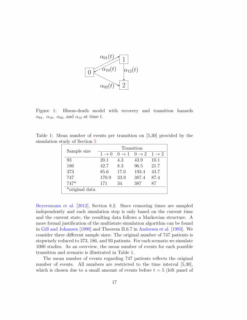
Figure 1: Illness-death model with recovery and transition hazardsα01, α10, α02, and α12 at time t.

Table 1: Mean number of events per transition on [5,30] provided by thesimulation study of Section 5

Sample sizeTransition

1→ 0 0→ 1 0→ 2 1→ 293 20.1 4.3 43.9 10.1186 42.7 8.3 96.5 21.7373 85.6 17.0 193.4 43.7747 170.9 33.9 387.4 87.4747* 171 34 387 87*original data

Beyersmann et al. [2012], Section 8.2. Since censoring times are sampledindependently and each simulation step is only based on the current timeand the current state, the resulting data follows a Markovian structure. Amore formal justification of the multistate simulation algorithm can be foundin Gill and Johansen [1990] and Theorem II.6.7 in Andersen et al. [1993]. Weconsider three different sample sizes: The original number of 747 patients isstepwisely reduced to 373, 186, and 93 patients. For each scenario we simulate1000 studies. As an overview, the mean number of events for each possibletransition and scenario is illustrated in Table 1.

The mean number of events regarding 747 patients reflects the originalnumber of events. All numbers are restricted to the time interval [5,30],which is chosen due to a small amount of events before t = 5 (left panel of

17

Figure 2). Further, less than 10% of all individuals are still under observationafter day 30. In particular, asymptotic approximations tend to be poor atthe left- and right-hand tails; cf. Remark 4.1(b) and Lin [1997].

Utilizing the R-package sde [Iacus, 2014], the quantiles cg1−α in (4.3) ofeach single study are empirically estimated by simulating 1000 sample pathsof a standard Brownian bridge. These quantiles are separately derived forboth the Aalen- and Greenwood-type variance estimates (2.5) and (2.6). Thebootstrap critical values are based on 1000 bootstrap realizations of W n foreach simulation step including both standard normal and centered Poissonvariates with variance one. The latter is motivated by a slightly better per-formance compared to standard normal multipliers (Beyersmann et al., 2013,and Dobler et al., 2015). Furthermore, Liu [1988] argued in a classical (linearregression) problem that wild bootstrap weights with skewness equal to onesatisfy the second order correctness of the resampling approach. Accordingto the cited simulation results, a similar result might hold true in our con-text, as the Poisson variates have skewness equal to one and standard normalvariates are symmetric. A careful analysis of the convergence rates, however,is certainly beyond the scope of this article. In order to guarantee statisticalreliability, we do not derive confidence bands for sample sizes and transitionswith a mean number of observed transitions distinctly smaller than 20. Thenominal level is set to α = 0.05. All simulations are performed with theR-computing environment version 3.3.2 [R Core Team, 2016].

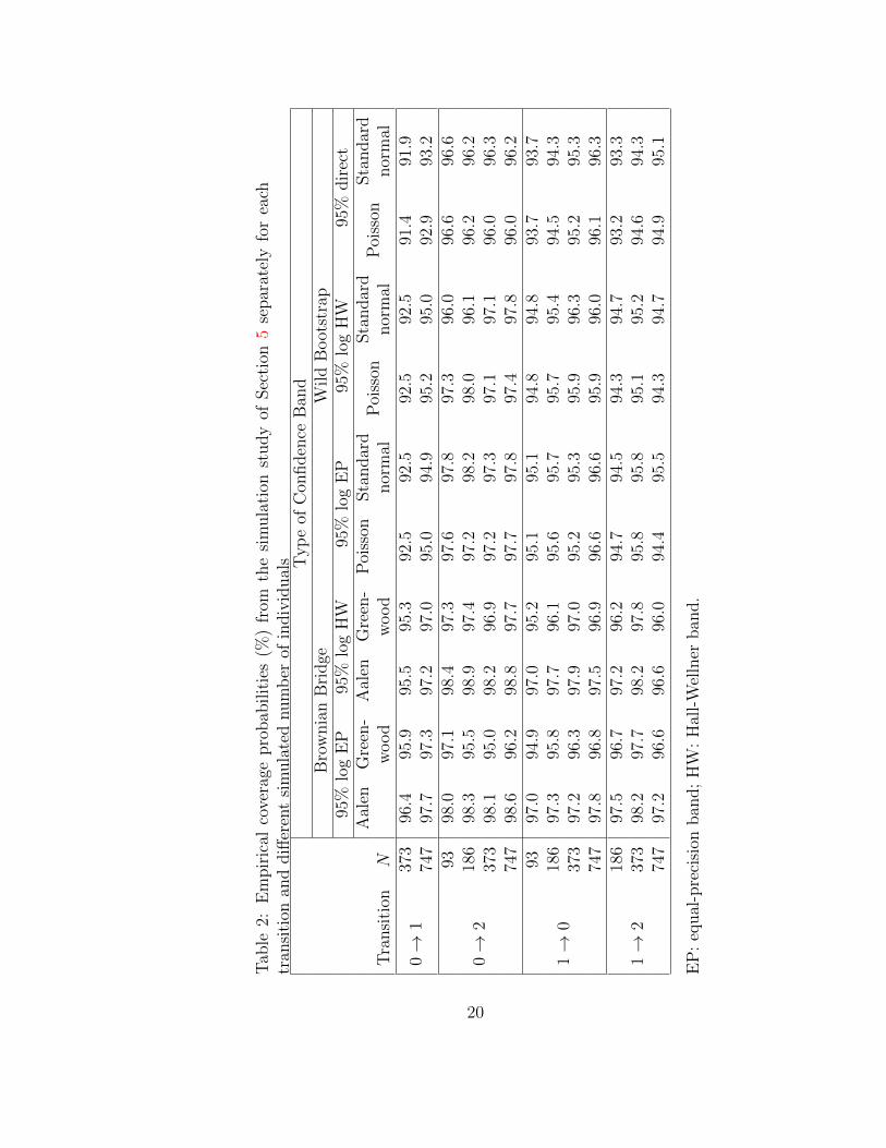
Following Table 2, almost all bands constructed via Brownian bridgesconsistently tend to be rather conservative in our setting, i.e., result in toobroad bands. Here, the usage of the Greenwood-type variance estimate yieldsmore accurate coverage probabilities compared to the Aalen-type estimate.In contrast, the wild bootstrap approach mostly outperforms the Brownianbridge procedures: The log-transformed wild bootstrap bands approximatelykeep the nominal level even in the smaller sample sizes, except for the 0→ 1transition with smallest sample size (corresponding to only 17 events in themean; cf. Table 1). We also observe that the log-transformation in generalimproves coverage for the wild bootstrap procedure. The current simulationstudy showed no clear preference for the choice of weight. Note that all wildbootstrap bands for transition 0 → 2 show a similar, but mostly reducedconservativeness compared to the bands provided by Brownian bridges. Wehave to emphasize that coverage probabilities for the cumulative hazard func-tions are drastically decreased to approximately 75% in all sample sizes iflog-transformed pointwise confidence intervals would wrongly be interpreted

18

time-simultaneously (results not shown).The second set of simulations follows the test for proportional hazards

derived in Theorem 4.2 with regard to keeping the preassigned error levelunder the null hypothesis. For that purpose, we assume a competing risksmodel with two competing events separately for two unpaired patient groups.For an illustration, see for instance, Figure 3.1 in Beyersmann et al. [2012].

We consider four different constant hazard scenarios: (I) the hazards for

the type-1 event are set to α(1)01 (t) = α

(2)01 (t) = 2 (no effect on the type-1 haz-

ard, in particular, a hazard ratio of c = 1); (II) α(1)01 (t) = 1 and α

(2)01 (t) = 2

(large effect); (III) α(1)01 (t) = α

(2)01 (t) = 1; (IV) α

(1)01 (t) = 1 and α

(2)01 (t) = 1.5

(moderate effect). In each scenario, we set α(1)02 = α

(2)02 (t) = 2, in particular,

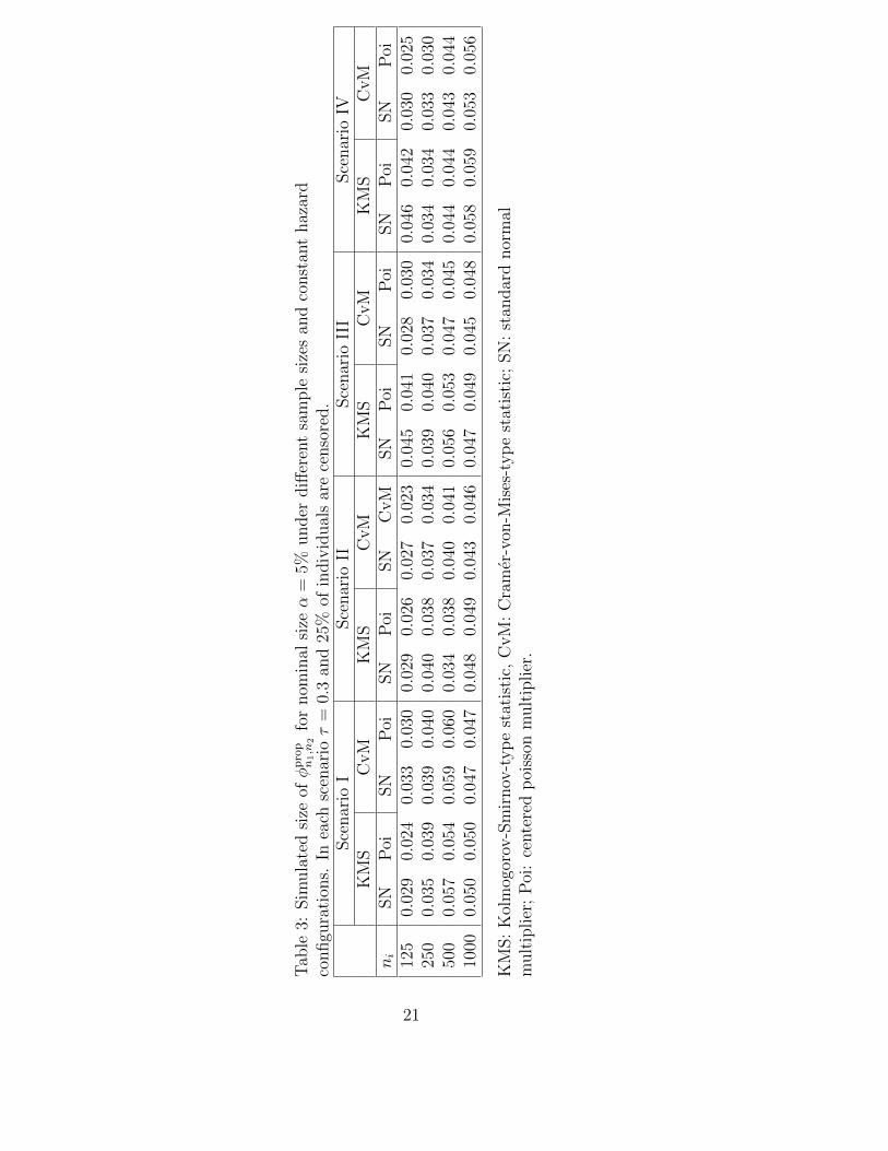
we consistently assume no group effect on the competing hazard. Further,scenario-specific administrative censoring times are chosen such that approx-imately 25% of the individuals are censored. The simulations designs areselected such that we include different effect sizes as well as different type-1 hazard ratio configurations with respect to the competing hazards. Weconsider a balanced design with n1 = n2 = n ∈ 125, 250, 500, 1000. Theright-hand tail of the domain of interest is set to τ = 0.3. Simulation ofthe event times and types follows the procedure explained in Chapter 3.2of Beyersmann et al. [2012]. As before, we simulate 1000 studies for eachscenario and sample size configuration, whereas the critical values of theKolmogorov-Smirnov-type and Cramer-von-Mises-type statistics from Sec-tion 4.3 are derived from 1000 bootstrap samples including both standardnormal and centered Poisson variates with variance one.

The results for the type I error rates (for α = 0.05) are displayed in Table3. As expected from consistency, the higher the number of patients the betteris the type I error approached for both test statistics in each scenario. Exceptfor Scenario (II), all procedures keep the type I error rate quite accuratelyfor n ≥ 500. For smaller sample sizes, all tests tend to be conservative witha particular advantage for the Kolmogorov-Smirnov statistic.

6 Data Example

The SIR-3 (Spread of Nosocomial I nfections and Resistant Pathogens) co-hort study at the Charite University Hospital in Berlin, Germany, prospec-tively collected data on the occurrence and consequences of hopital-aquiredinfections in intensive care [Beyersmann et al., 2006, Wolkewitz et al., 2008].

19

Tab

le2:

Em

pir

ical

cove

rage

pro

bab

ilit

ies

(%)

from

the

sim

ula

tion

study

ofSec

tion

5se

par

atel

yfo

rea

chtr

ansi

tion

and

diff

eren

tsi

mula

ted

num

ber

ofin

div

idual

s Typ

eof

Con

fiden

ceB

and

Bro

wnia

nB

ridge

Wild

Boot

stra

p95

%lo

gE

P95

%lo

gH

W95

%lo

gE

P95

%lo

gH

W95

%dir

ect

Aal

enG

reen

-A

alen

Gre

en-

Poi

sson

Sta

ndar

dP

oiss

onSta

ndar

dP

oiss

onSta

ndar

dT

ransi

tion

Nw

ood

wood

nor

mal

nor

mal

nor

mal

0→

137

396

.495

.995

.595

.392

.592

.592

.592

.591

.491

.974

797

.797

.397

.297

.095

.094

.995

.295

.092

.993

.2

0→

2

9398

.097

.198

.497

.397

.697

.897

.396

.096

.696

.618

698

.395

.598

.997

.497

.298

.298

.096

.196

.296

.237

398

.195

.098

.296

.997

.297

.397

.197

.196

.096

.374

798

.696

.298

.897

.797

.797

.897

.497

.896

.096

.2

1→

0

9397

.094

.997

.095

.295

.195

.194

.894

.893

.793

.718

697

.395

.897

.796

.195

.695

.795

.795

.494

.594

.337

397

.296

.397

.997

.095

.295

.395

.996

.395

.295

.374

797

.896

.897

.596

.996

.696

.695

.996

.096

.196

.3

1→

218

697

.596

.797

.296

.294

.794

.594

.394

.793

.293

.337

398

.297

.798

.297

.895

.895

.895

.195

.294

.694

.374

797

.296

.696

.696

.094

.495

.594

.394

.794

.995

.1

EP

:eq

ual

-pre

cisi

onban

d;

HW

:H

all-

Wel

lner

ban

d.

20

Tab

le3:

Sim

ula

ted

size

ofφprop

n1,n

2fo

rnom

inal

sizeα

=5%

under

diff

eren

tsa

mple

size

san

dco

nst

ant

haz

ard

configu

rati

ons.

Inea

chsc

enar

ioτ

=0.

3an

d25

%of

indiv

idual

sar

ece

nso

red.

Sce

nar

ioI

Sce

nar

ioII

Sce

nar

ioII

ISce

nar

ioIV

KM

SC

vM

KM

SC

vM

KM

SC

vM

KM

SC

vM

ni

SN

Poi

SN

Poi

SN

Poi

SN

CvM

SN

Poi

SN

Poi

SN

Poi

SN

Poi

125

0.02

90.

024

0.03

30.

030

0.02

90.

026

0.02

70.

023

0.04

50.

041

0.02

80.

030

0.04

60.

042

0.03

00.

025

250

0.03

50.

039

0.03

90.

040

0.04

00.

038

0.03

70.

034

0.03

90.

040

0.03

70.

034

0.03

40.

034

0.03

30.

030

500

0.05

70.

054

0.05

90.

060

0.03

40.

038

0.04

00.

041

0.05

60.

053

0.04

70.

045

0.04

40.

044

0.04

30.

044

1000

0.05

00.

050

0.04

70.

047

0.04

80.

049

0.04

30.

046

0.04

70.

049

0.04

50.

048

0.05

80.

059

0.05

30.

056

KM

S:

Kol

mog

orov

-Sm

irnov

-typ

est

atis

tic,

CvM

:C

ram

er-v

on-M

ises

-typ

est

atis

tic;

SN

:st

andar

dnor

mal

mult

iplier

;P

oi:

cente

red

poi

sson

mult

iplier

.

21

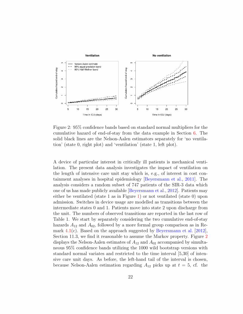
Figure 2: 95% confidence bands based on standard normal multipliers for thecumulative hazard of end-of-stay from the data example in Section 6. Thesolid black lines are the Nelson-Aalen estimators separately for ‘no ventila-tion’ (state 0, right plot) and ‘ventilation’ (state 1, left plot).

A device of particular interest in critically ill patients is mechanical venti-lation. The present data analysis investigates the impact of ventilation onthe length of intensive care unit stay which is, e.g., of interest in cost con-tainment analyses in hospital epidemiology [Beyersmann et al., 2011]. Theanalysis considers a random subset of 747 patients of the SIR-3 data whichone of us has made publicly available [Beyersmann et al., 2012]. Patients mayeither be ventilated (state 1 as in Figure 1) or not ventilated (state 0) uponadmission. Switches in device usage are modelled as transitions between theintermediate states 0 and 1. Patients move into state 2 upon discharge fromthe unit. The numbers of observed transitions are reported in the last row ofTable 1. We start by separately considering the two cumulative end-of-stayhazards A12 and A02, followed by a more formal group comparison as in Re-mark 4.1(c). Based on the approach suggested by Beyersmann et al. [2012],Section 11.3, we find it reasonable to assume the Markov property. Figure 2displays the Nelson-Aalen estimates of A12 and A02 accompanied by simulta-neous 95% confidence bands utilizing the 1000 wild bootstrap versions withstandard normal variates and restricted to the time interval [5,30] of inten-sive care unit days. As before, the left-hand tail of the interval is chosen,because Nelson-Aalen estimation regarding A12 picks up at t = 5, cf. the

22

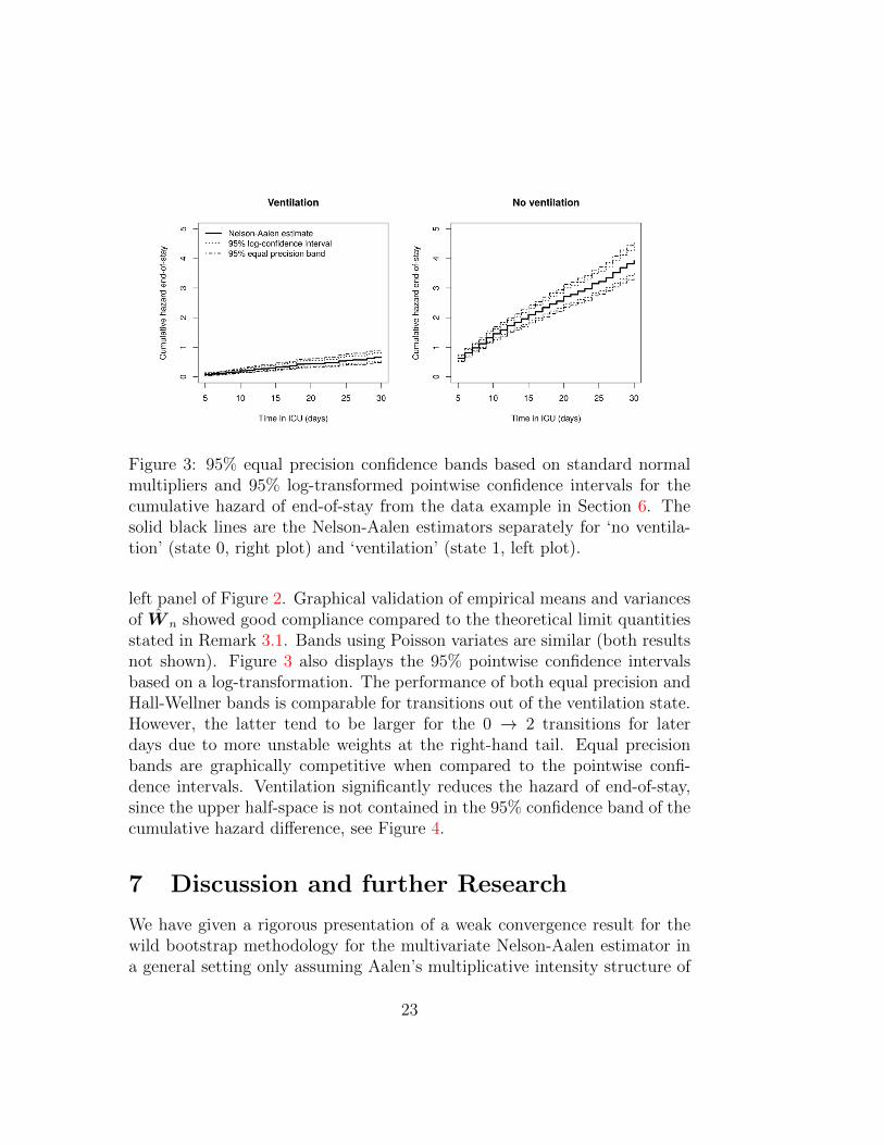
Figure 3: 95% equal precision confidence bands based on standard normalmultipliers and 95% log-transformed pointwise confidence intervals for thecumulative hazard of end-of-stay from the data example in Section 6. Thesolid black lines are the Nelson-Aalen estimators separately for ‘no ventila-tion’ (state 0, right plot) and ‘ventilation’ (state 1, left plot).

left panel of Figure 2. Graphical validation of empirical means and variancesof W n showed good compliance compared to the theoretical limit quantitiesstated in Remark 3.1. Bands using Poisson variates are similar (both resultsnot shown). Figure 3 also displays the 95% pointwise confidence intervalsbased on a log-transformation. The performance of both equal precision andHall-Wellner bands is comparable for transitions out of the ventilation state.However, the latter tend to be larger for the 0 → 2 transitions for laterdays due to more unstable weights at the right-hand tail. Equal precisionbands are graphically competitive when compared to the pointwise confi-dence intervals. Ventilation significantly reduces the hazard of end-of-stay,since the upper half-space is not contained in the 95% confidence band of thecumulative hazard difference, see Figure 4.

7 Discussion and further Research

We have given a rigorous presentation of a weak convergence result for thewild bootstrap methodology for the multivariate Nelson-Aalen estimator ina general setting only assuming Aalen’s multiplicative intensity structure of

23

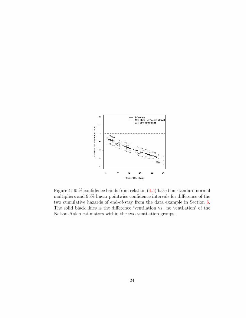
Figure 4: 95% confidence bands from relation (4.5) based on standard normalmultipliers and 95% linear pointwise confidence intervals for difference of thetwo cumulative hazards of end-of-stay from the data example in Section 6.The solid black lines is the difference ‘ventilation vs. no ventilation’ of theNelson-Aalen estimators within the two ventilation groups.

24

the underlying counting processes. This allowed the construction of time-simultaneous confidence bands and intervals as well as asymptotically validequivalence and equality tests for cumulative hazard functions. In the contextof time-to-event analysis, our general framework is not restricted to the stan-dard survival or competing risks setting, but also covers arbitrary Markovianmultistate models with finite state space, other classes of intensity models likerelative survival or excess mortality models, and even specific semi-Markovsituations. Additionally, independent left-truncation and right-censoring canbe incorporated. The procedure has also been used to construct a test forproportional hazards. Easy and computationally convenient implementationand within- or two-sample comparisons demonstrate its attractiveness in var-ious practical applications.

Future work will be on the approximation of the asymptotic distributioncorresponding to the matrix of transition probabilities (see Aalen and Jo-hansen, 1978) and functionals thereof in general Markovian multistate mod-els. This is of great practical interest, because no similar Brownian Bridgeprocedure is available to perform time-simultaneous statistical inference. Inparticular, previous implications rely on pointwise considerations. Note thatsuch an approach would significantly simplify the original justifications givenby Lin [1997] and generalizes his idea mainly used in the context of competingrisks [Scheike and Zhang, 2003, Hyun et al., 2009, Beyersmann et al., 2013].In addition, we plan to extend the utilized wild bootstrap technique to gen-eral semiparametric regression models; see Lin et al. [2000] for an applicationin the survival context. Current work investigates to which degree the mar-tingale properties presented in this article may be exploited to obtain wildbootstrap consistencies for such functionals of Nelson-Aalen estimates or forestimators in semiparametric regression models. We are confident that thepresent approach will lead to reliable inference procedures in these contextsfor which there has been only little research on such general methodology.

In contrast to the procedure of Schoenfeld et al. [2002] and other recentpublications mentioned in the introduction, the more general illness-deathmodel with recovery does not rely on a constant hazards assumption andcaptures both the time-dependent structure of mechanical ventilation andthe competing event ‘death in ICU’. This significantly improves medical in-terpretations. The widths of the confidence bands were competitive com-pared to the pointwise confidence intervals, i.e., demonstrated usefulness inpractical situations. Applications of our theory are not restricted to studiesinvestigating mechanical ventilation, but may also be helpful to investigate,

25

for instance, the impact of immunosuppressive therapy in leukemia diagnosedpatients [cf. Schmoor et al., 2013]. The proposed procedure has even beenapplied in a recent study investigating femoral fracture risk in an elderlypopulation [Bluhmki et al., 2016].

It has to be emphasized that our simulation study suggested that thewild bootstrap approach leads to more powerful procedures (i.e. to narrowerconfidence bands) compared to the approximation via Brownian bridges.As expected, the applied log-transformation results in improved small sampleproperties compared to the untransformed wild bootstrap bands. Based onthe current simulation study, however, it was difficult to clearly recommendwhich type of band and which type of multiplier should be used.

A Proofs

Proof of Lemma 3.1. Due to similarity, it is enough to concentrate at thefirst component only; thus, we subsequently suppress the subscript ‘1’. Theindependence of all white noise processes immediately imply the orthogonal-ity of all component processes. At first, we verify the martingale property;the square-integrability is obviously fulfilled since E(G2

1(0)) < ∞. To thisend, let 0 ≤ s ≤ t. By measurability of the counting and the predictableprocess with respect to C0, we have

E(Wn(t) | Cs) =√n

∫(0,t]

J(u)

Y (u)E(G(u) | Cs) dN(u)

=√n

∫(0,s]

J(u)

Y (u)G(u) dN(u) +

√n

∫(s,t]

J(u)

Y (u)E(G(u)) dN(u) = Wn(s)

by the independence of σ(G(u)) and Cs for all u > s. Hence, the martingaleproperty is shown.

The predictable variation process 〈Wn〉 is the compensator of W 2n , i.e. we

26

calculate

E(W 2n(t) | Cs)

= n(∫

(0,s]

∫(0,s]

+

∫(s,t]

∫(0,s]

+

∫(0,s]

∫(s,t]

+

∫(s,t]

∫(s,t]

)E(G(u)G(v) | Cs)

× J(u)J(v)

Y (u)Y (v)dN(u) dN(v)

= n(∫

(0,s]

∫(0,s]

G(u)G(v) +

∫(s,t]

∫(0,s]

E(G(u))G(v)

+

∫(0,s]

∫(s,t]

G(u)E(G(v)) +

∫(s,t]

∫(s,t]

E(G(u)G(v))) J(u)J(v)

Y (u)Y (v)dN(u) dN(v)

= n(∫

(0,s]

∫(0,s]

G(u)G(v)J(u)J(v)

Y (u)Y (v)dN(u)dN(v) +

∫(s,t]

E(G2(u))J(u)

Y 2(u)dN(u)

)= W 2

n(s) + n

∫(0,t]

J(u)

Y 2(u)dN(u)− n

∫(0,s]

J(u)

Y 2(u)dN(u),

again by the Cs-measurability of G(u) for u ≤ s and their independence foru > s. The second to last equality is due to the independence of G(u) and

G(v) for u 6= v. Hence, (W 2n(t)− n

∫(0,t]

J(u)Y 2(u)

dN(u))t∈[0,τ ] is a martingale.

Letting ∆f denote the jump-size process fo a cadlag function f , the def-inition of the optional variation process yields

[Wn](t) =∑0<s≤t

(∆Wn(s))2 = n∑0<s≤t

G2(u)J(u)

Y 2(u)∆N(u) = n

∫(0,t]

G2(u)J(u)

Y 2(u)dN(u),

where the sum is taken over all jump points of N .

Proof of Theorem 3.1. It is enough to verify the conditions of Rebolledo’smartingale central limit theorem (in conditional probability); see e.g. The-orem II.5.1 in Andersen et al. [1993]. Since the filtration C0 at time s = 0is not trivial, the resulting weak convergence will hold given C0 as well, inprobability. From the classical theory we know that the Aalen-type vari-ance estimator, which is in fact the predictable variation process of Wn, isuniformly consistent for the variance function.

It remains to prove the Lindeberg condition (2.5.3) on page 83 in Andersenet al. [1993]. But, by the same arguments as in the proof of Lemma 3.1, this isexactly the same as the Lindeberg condition for the Nelson-Aalen estimatoritself. And this holds due to the main assumption (2.2).

27

Hence, Rebolledo’s martingale central limit theorem yields the desiredweak convergence as well as the uniform consistency of the optional variationprocess.

Proof of Theorem 4.1. For convergence (4.1), see Section IV.1 in Andersenet al. [1993] in combination with Slutsky’s theorem. Convergence (4.2) fol-lows from the consistency of σ∗2, Slutsky’s theorem and Theorem 3.1, sinceWn asymptotically mimicks the distribution of

√n(An −A). The functional

delta-method for (x 7→ log x) completes the proof.

Proof of Corollaries 4.1 and 4.3. Due to the continuous limit distributionthe conditional quantiles converge as well in probability; see e.g. Janssenand Pauls [2003], Lemma 1. The consistency of ϕKSn under K 6= follows fromthe convergence in probability of the conditional quantile towards a finitevalue and from the uniform consistency of the multivariate Nelson-Aalenestimator for the cumulative hazard functions. Since the factor

√n tends to

infinity, the test statistic also goes to infinity in probability under K 6=.

Proof of Corollary 4.2. The proof extends the arguments of Wellek [2010],Section 3.1, from confidence intervals to confidence bands. Write H = H1 ∪H2 where

H1 : A(s) ≤ A0(s)− `(s) for some s ∈ [t1, t2]and H2 : A(s) ≥ A0(s) + u(s) for some s ∈ [t1, t2].

SupposeH is true and let without loss of generality beH1 true due to analogy.Then the probability of a false rejection of H amounts to

P (A0(s)− `(s) < an(s) and bn(s) < A0(s) + u(s) for all s ∈ [t1, t2])

≤ P (A0(s)− `(s) < an(s) for all s ∈ [t1, t2])

≤ P (A(s) < an(s) for some s ∈ [t1, t2]) −→ α.

Here the last inequality holds since H1 is true and the convergence is due tothe asymptotic coverage probability of the confidence band (an(s),∞)s∈[t1,t2].

In order to prove consistency, suppose the alternative hypothesis K istrue and choose any ε such that

0 < ε < infs∈[t1,t2]

−(A0(s)− `(s)− A(s)) ∧ (A0(s) + u(s)− A(s)).

28

Thus, by the (uniform) consistency of the Nelson-Aalen estimator and thewild bootstrap quantiles, the probability of a correct rejection of H equals

P (A0(s)− `(s) < an(s) and bn(s) < A0(s) + u(s) for all s ∈ [t1, t2])

≥ P (A(s)− ε < an(s) and bn(s) < A(s) + ε for all s ∈ [t1, t2]) −→ 1

as n → ∞. For the convergence in the previous display, also note that

anP−−→ A as well as bn

P−−→ A uniformly in [t1, t2].

Proof of Theorem 4.2. Let t0 > 0. Denote by D>0[t0, τ ] ⊂ D[t0, τ ] the coneof positive cadlag functions that are bounded away from zero. It is easy tosee that the functional φ : D2

>0[t0, τ ]→ D>0[t0, τ ], (f, g) 7→ fg

is Hadamard-

differentiable tangentially to the set of pairs of continuous functions C2[t0, τ ]with continuous and linear Hadamard-derivative

φ′(f,g) : C2[t0, τ ]→ C[t0, τ ], (h1, h2) 7−→h1g− h2

f

g2.

A simpler Hadamard-differentiability result holds for φ’s restriction to τ ,i.e. φ|τ : (0,∞)2 3 (f(τ), g(τ)) 7→ f(τ)

g(τ)with continuous, linear Hadamard-

derivative

(φ|τ )′(f,g) : R2 → R, (h1(τ), h2(τ)) 7−→ h1(τ)

g(τ)− h2(τ)

f(τ)

g2(τ).

Hence, we apply the functional δ-method and the continuous mappingtheorem to√n1n2

n(φ(A(2)

n2, A(1)

n1)−φ(A(2), A(1))) and φ′

(A(2)n2,A

(1)n1

)

(√n1

nW (2)n2,

√n2

nW (1)n1

),

respectively, verifying their equality in distribution in the limit (conditionallyin probability for the latter). Proceed similarly with the restricted functionalφ|τ . Furthermore, the difference functional of both above functionals retainsthe Hadamard-differentiability tangentially to the set of pairs of continuousfunctions. Our specific choices of the distance ρ are continuous function-als, hence we are able to apply the continuous mapping theorem again. Toconclude the proof of the asymptotic behaviour of ϕprop

n1,n2under Hprop

0 , notethat the particular weight function solves the problem of dividing by zero att0 = 0.

29

For the asymptotic power assertion, let t1 ∈ [0, τ ] at which Hprop0 is vio-

lated. Then

ρ( A

(2)n2

A(1)n1

,A

(2)n2 (τ)

A(1)n1 (τ)

)converges in probability to a positive value, whence Tn1,n2

p→∞ follows. Theconditional quantiles, however, still converge to a finite constant in probabil-ity by the above arguments.

B Supplementary Material: Alternative Proof

of Theorem 3.1

Before proving the conditional convergence in distribution stated in Theo-rem 3.1, we extend the conditional central limit theorem (CCLT) A.1 givenBeyersmann et al. [2013] to our context. For that purpose, consider N(τ) =∑k

j=1Nj(τ) as the random number of totally observed jumps in [0, τ ]. Due tothe general framework only assuming Aalen’s multiplicative intensity model,random sums with a random number N of summands occur and need to beanalyzed, since each jump of the counting processes requires its own multi-plier Gj(u) in the resampling scheme. Thus, we state a more general CCLTas given in Beyersmann et al. [2013], where ‖ · ‖ denotes the Euclidean normon Rp, p ∈ N. L again denotes the law.

Throughout, the resampled quantities are modelled via projection on aproduct probability space (Ω1×Ω2,A1⊗A2, P1⊗P2), where the white noiseprocesses only depend on the second and the data only on the first coordinate.

Theorem B.1. Let Zn;l : (Ω1,A1, P1) → (Rp,Bp), l = 1, . . . , N, be a tri-angular array of Rp random variables, p ∈ N, where N : (Ω1,A1, P1) →(N0,P(N0)) is an integer-valued random variable, non-decreasing in n, such

that NP→ ∞ as n → ∞. Let Gn;l : (Ω2,A2, P2) → (R,B), l ∈ N, be rowwise

i.i.d. random variables with E(Gn;1) = 0 and var(Gn;1) = 1. Modelled onthe product space (Ω1 × Ω2,A1 ⊗ A2, P1 ⊗ P2), the arrays (N,Zn;l : l ≤ N)

30

and (Gn;l)l∈N are independent. Suppose that Zn;l fulfills the convergences

max1≤l≤N

‖Zn;l‖P−→ 0 (B.1)

N∑l=1

Zn;lZ′n;l

P−→ Γ, (B.2)

where Γ is a positive definite covariance matrix. Then, conditionally given(N,Zn;l : l ≤ N), the following weak convergence holds in probability:

L( N∑l=1

Gn;lZn;l

∣∣∣ N,Zn;l : l ≤ N)

d−→ N(0,Γ). (B.3)

Proof. SinceN is non-decreasing in n withNP→∞, it follows thatN(ω1, ω2)→

∞ for P1-almost all ω1 ∈ Ω1, independently of the value ω2 ∈ Ω2. Thus,for P1-almost all such fixed ω1 ∈ Ω1, we have a deterministic number ofsummands N(ω1, ·). By the subsequence principle, choose a subsequence(n′) ⊆ (n) = N along which (B.1) and (B.2) hold for almost every ω1 ∈ Ω1 aswell. Applying the CCLT A.1 in Beyersmann et al. [2013] with its conditionsbeing almost surely fulfilled, the weak convergence (B.3) follows P1-almostsurely along n′. A further application of the subsequence principle, goingback to convergence in probability, completes the proof.

Proof of Theorem 3.1. Conditional Finite-Dimensional Convergence of Wn.Due to asymptotic mutual independence, we only consider the first entry W1n

of W n and suppress the subscript ‘1’ subsequently. Define countably manyi.i.d. random variables Gn;1, Gn;2, . . . with E(Gn;1) = 0 and var(Gn;1) = 1,that are independent of Cn, and define processes Zn;1, . . . , Zn;N(τ) such thatequation (3.2) is re-expressed as

Wn(t) =∑v∈T

G(v)√nXv(t)

d=

N(τ)∑l=1

Gn;lZn;l(t), (B.4)

whered= denotes equality in distribution. HereXv(t) := 1v ≤ t∆N(v)/Y (v)

and T = u ∈ [0, τ ] | ∆N(u) = 1 contains all jump times of the countingprocess N . Then, the general framework of Theorem B.1 is fulfilled for thetriangular array Zn;l(tj), l = 1, . . . , N(τ), j = 1, . . . , r, for any finite subset

31

t1, . . . , tr ⊂ [0, τ ]. Next, conditions (B.1) and (B.2) are verified in a similarmanner as in Beyersmann et al. [2013]. Applying the subsequence principlefor convergence in probability to assumption (2.2), it follows that for everysubsequence there exists a further subsequence, say n, such that as n→∞

supu∈[0,τ ]

∣∣∣Y (u)

n− y(u)

∣∣∣ a.s.−−−→ 0, (B.5)

i.e., the left-hand side converges to zero for P1-almost all ω ∈ Ω1. Fixan arbitrarily small ε > 0 and an ω for which (B.5) holds. The followingarguments implicitly consider all n ≥ n0(ω, ε) for an n0 determined by (B.5).Hence, the left-hand side of (B.5) is less than ε for all such n ≥ n0. Choosea γε = γε(ω) > 0 such that

supu∈[0,τ ]

n

Y (ω, u)≤ γεy(u)

≤ γεinf

v∈[0,τ ]y(v)

=: cε.

Since Xv is (at most) a one-jump process on [0, τ ], we have

supl=1,...,N(τ)

supt∈[0,τ ]

|Zn;l(t)| ≤√n sup

v∈TXv(ω, τ) ≤ n−1/2

n

Y (ω, τ)≤ n−1/2cε

n→∞−−−→ 0.

In particular, Z n;l = (Zn;l(t1), . . . , Zn;l(tk))′ satisfies max

1≤l≤N(τ)‖Z n;l(t)‖

P−→ 0,

and (B.1) holds.For simplicity, condition (B.2) is only shown for two time points 0 ≤ t1 ≤

t2 ≤ τ , such that Z n;l = (Zn;l(t1), Zn;l(t2))′. Representation (B.4) implies

that

N(τ)∑l=1

Z n;lZ′n;l = n

∑v∈T

(X2v (t1) Xv(t1)Xv(t2)

Xv(t1)Xv(t2) X2v (t2)

).

The off-diagonals equal Xv(t1)Xv(t2) = 1v ≤ t1∆N(v)/Y 2(v) and theother two components are obtained for t1 = t2. Using the Doob-Meyerdecomposition (2.1), it follows that

n∑v∈T

Xv(t1)Xv(t2) = n−1∫(0,t1]

( n

Y (u)

)2dM(u) +

∫(0,t1]

n

Y (u)α(u)du.

32

As in Beyersmann et al. [2013], Rebolledo’s martingale central limit theorem(Andersen et al., 1993, Theorem II.5.1) shows the negligibility of the martin-gale integral. The remaining integral converges to ψ(t1, t2) =

∫(0,t1]

α(u)/y(u)du

in probability due to assumption (B.5). Consequently, we conclude that, asn→∞,

N(τ)∑l=1

Z n;lZ′n;l

P−−→(ψ(t1, t1) ψ(t1, t2)ψ(t1, t2) ψ(t2, t2)

).

Let U be a zero-mean Gaussian process with covariance function ψ. Ex-tending previous arguments to r ∈ N time points t1, . . . , tr, Theorem B.1implies, conditionally on Cn, the finite-dimensional weak convergence

(Wn(t1), . . . , Wn(tr))′ d−→ (U(t1), . . . , U(tr))

′

in probability. Conditionally on Cn, only the white noise processes G1, . . . , Gk

in (3.2) are random and, in particular, stochastically independent. Thisimplies the multivariate conditional weak convergence

(W n(t1), . . . ,W n(tr))′ d−→ (U (t1), . . . ,U (tr))

′ in probability,

where U = (U1, . . . , Uk)′ has independent components and the asserted co-

variance structure.

The conditional tightness of Wn follows similarly as in the proof of The-orem 3.1 in Dobler and Pauly [2014]. As previously, tightness of W n isseparately studied for each single component, i.e., we only consider Wjn andsuppress the subscript ‘j’ of the estimators and counting processes as above.Let 0 ≤ r ≤ s ≤ t ≤ τ . Then, Theorem 15.6 in Billingsley [1968] using γ = 2and α = 1 in combination with the remark on p. 356 in Jacod and Shiryaev[2003] leads us to the following conditional expectation:

E[(Wn(t)− Wn(s))2(Wn(s)− Wn(r))2 | C0]

= n2E[( ∫

(s,t]

G(u)J(u)

Y (u)dN(u)

)2( ∫(r,s]

G(v)J(v)

Y (v)dN(v)

)2 ∣∣∣ C0]= n2

∫(s,t]

∫(s,t]

∫(r,s]

∫(r,s]

J(u1)

Y (u1)

J(u2)

Y (u2)

J(v1)

Y (v1)

J(v2)

Y (v2)

× E[G(u1)G(u2)G(v1)G(v2)]dN(v2)dN(v1)dN(u2)dN(u1).

33

Since the multipliers G(u), u ∈ T are independent and the intervals (r, s]and (s, t] are disjoint, the remaining expectation decomposes into a productof E[G(u)] or E[G2(u)]. Here, each expectation of a multiplier to the powerof one vanishes due to E[G(u)] = 0 and a multiplier to the power of two onlyoccurs whenever u1 = u2 ∈ T or v1 = v2 ∈ T . Since E[G2(u)] = 1, the abovedisplay simplifies to

n2

∫(s,t]

J(u)

Y (u)2dN(u)

∫(r,s]

J(v)

Y (v)2dN(v) = [σ2(t)− σ2(s)][σ2(s)− σ2(r)] ≤ [σ2(t)− σ2(r)]2

with σ2 defined as in (2.5). By Theorem IV.1.2 in Andersen et al. [1993] theconvergence in probability of the right-hand side to (σ2(t) − σ2(r))2 holdsuniformly in r, t ∈ [0, τ ]. Following the lines of Dobler and Pauly [2014] byutilizing the proposition in Jacod and Shiryaev [2003], p. 356, conditionaltightness is shown along subsubsequences almost surely. Another applicationof the subsequence principle shows the stated result.

Acknowledgements

Jan Beyersmann was supported by Grant BE 4500/1-1 of the German Re-search Foundation (DFG).

References

O. O. Aalen. Nonparametric inference for a family of counting processes.The Annals of Statistics, 6(4):701–726, 1978.

O. O. Aalen and S. Johansen. An empirical transition matrix for non-homogeneous Markov chains based on censored observations. ScandinavianJournal of Statistics, 5(3):141–150, 1978.

O. O. Aalen, Ø. Borgan, and H. K. Gjessing. Survival and Event HistoryAnalysis: A Process Point of View. Springer, New York, 2008.

M. G. Akritas. Bootstrapping the Kaplan-Meier estimator. Journal of theAmerican Statistical Association, 81(396):1032–1038, 1986.

34

A. Allignol, M. Schumacher, C. Wanner, C. Drechsler, and J. Beyersmann.Understanding competing risks: a simulation point of view. BMC MedicalResearch Methodology, 11(86), 2011.

P. K. Andersen and M. Væth. Simple parametric and nonparametric modelsfor excess and relative mortality. Biometrics, 45(2):523–535, 1989.

P. K. Andersen, Ø. Borgan, R. D. Gill, and N. Keiding. Statistical ModelsBased on Counting Processes. Springer, New York, 1993.

R. Bajorunaite and J. P. Klein. Two-sample tests of the equality of twocumulative incidence functions. Computational Statistics & Data Analysis,51(9):4269–4281, 2007.

J. Beyersmann, P. Gastmeier, H. Grundmann, S. Barwolff, C. Geffers,M. Behnke, H. Ruden, and M. Schumacher. Use of multistate models toassess prolongation of intensive care unit stay due to nosocomial infection.Infection Control and Hospital Epidemiology, 27(05):493–499, 2006.

J. Beyersmann, M. Wolkewitz, A. Allignol, N. Grambauer, and M. Schu-macher. Application of multistate models in hospital epidemiology: ad-vances and challenges. Biometrical Journal, 53(2):332–350, 2011.

J. Beyersmann, A. Allignol, and M. Schumacher. Competing Risks and Mul-tistate Models with R. Springer, New York, 2012.

J. Beyersmann, S. Di Termini, and M. Pauly. Weak convergence of the wildbootstrap for the Aalen-Johansen estimator of the cumulative incidencefunction of a competing risk. Scandinavian Journal of Statistics, 40(3):387–402, 2013.

P. J. Bickel and D. A. Freedman. Some asymptotic theory for the bootstrap.The Annals of Statistics, 9(6):1196–1217, 1981.

O. Bie, Ø. Borgan, and K. Liestøl. confidence intervals and confidence bandsfor the cumulative hazard rate function and their small sample properties.Scandinavian Journal of Statistics, 14(3):221–233, 1987.

P. Billingsley. Convergence of Probability Measures. Wiley, New York, 1stedition, 1968.

35

Tobias Bluhmki, Raphael Simon Peter, Kilian Rapp, Hans-Helmut Konig,Clemens Becker, Ivonne Lindlbauer, Dietrich Rothenbacher, Jan Beyers-mann, and Gisela Buchele. Understanding mortality of femoral fracturesfollowing low-impact trauma in persons with and without care need. Jour-nal of the American Medical Directors Association, 2016.

D. Cox. Regression models and life tables (with discussion). Journal of theRoyal Statistical Society, 34:187–220, 1972.

M. A. Q. Curley, D. Wypij, R. S. Watson, M. J. C. Grant, L. A. Asaro,I. M. Cheifetz, B. L. Dodson, L. S. Franck, R. G. Gedeit, D. C. Angus,M. A. Matthay, and for the RESTORE Study Investigators and the PALISINetwork. Protocolized sedation vs usual care in pediatric patients mechan-ically ventilated for acute respiratory failure: a randomized clinical trial.Journal of the American Medical Association, 313(4):379–389, 2015.

M. de Wit, C. Gennings, W. I. Jenvey, and S. K. Epstein. Randomizedtrial comparing daily interruption of sedation and nursing-implementedsedation algorithm in medical intensive care unit patients. Critical Care,12(3):R70, 2008.

D. Dobler and M. Pauly. Bootstrapping Aalen-Johansen processes for com-peting risks: handicaps, solutions, and limitations. Electronic Journal ofStatistics, 8(2):2779–2803, 2014.

D. Dobler, J. Beyersmann, and M. Pauly. Non-strange weird resampling forcomplex survival data. submitted article; arXiv preprint arXiv:1507.02838,2015.

A. Dudek, M. Gocwin, and J. Leskow. Simultaneous confidence bands for theintegrated hazard function. Computational Statistics, 23(1):41–62, 2008.

B. Efron. Bootstrap methods: another look at the jackknife. The Annals ofStatistics, 7(1):1–26, 1979.

B. Efron. Censored data and the bootstrap. Journal of the American Sta-tistical Association, 76(374):312–319, 1981.

R. Gill and M. Schumacher. A simple test of the proportional hazards as-sumption. Biometrika, 74(2):289–300, 1987.

36

R. D. Gill and S. Johansen. A survey of product-integration with a viewtoward application in survival analysis. The Annals of Statistics, 18(4):1501–1555, 1990.

D. V. Glidden. Robust Inference for Event Probabilities with Non-MarkovEvent Data. Biometrics, 58(2):361–368, 2002.

P. I. Good. Permutation, Parametric, and Bootstrap Tests of Hypotheses.Springer, New York, 3rd edition, 2005.

P. M. Grambsch and T. M. Therneau. Proportional hazards tests and diag-nostics based on weighted residuals. Biometrika, 81(3):515–526, 1994.

P. Hall and S. R. Wilson. Two guidelines for bootstrap hypothesis testing.Biometrics, 47(2):757–762, 1991.

Wendy J Hall and Jon A Wellner. Confidence bands for a survival curve fromcensored data. Biometrika, 67(1):133–143, 1980.

K. R. Hess. Graphical methods for assessing violations of the proportionalhazards assumption in Cox regression. Statistics in medicine, 14(15):1707–1723, 1995.

S. Hieke, H. Bertz, M. Dettenkofer, M. Schumacher, and J. Beyersmann.Initially fewer bloodstream infections for allogeneic vs. autologous stem-cell transplants in neutropenic patients. Epidemiology and Infection, 141(01):158–164, 2013.

L. Horvath and B. S. Yandell. Convergence rates for the bootstrappedproduct-limit process. The Annals of Statistics, 15(3):1155–1173, 1987.

S. Hyun, Y. Sun, and R. Sundaram. Assessing cumulative incidence functionsunder the semiparametric additive risk model. Statistics in Medicine, 28(22):2748–2768, 2009.

Stefano Maria Iacus. sde: simulation and inference for stochastic differentialequations, 2014. URL https://CRAN.R-project.org/package=sde. Rpackage version 2.0.13.

J. Jacod and A. N. Shiryaev. Limit theorems for stochastic processes.Springer, Berlin, 2nd edition, 2003.

37

A. Janssen and T. Pauls. How do bootstrap and permutation tests work?The Annals of Statistics, 31(3):768–806, 2003.

James A Koziol and David P Byar. Percentage points of the asymptoticdistributions of one and two sample K-S statistics for truncated or censoreddata. Technometrics, 17(4):507–510, 1975.

D. Kraus. Data-driven smooth tests of the proportional hazards assumption.Lifetime data analysis, 13(1):1–16, 2007.

D. Y. Lin. Goodness-of-fit analysis for the Cox regression model based on aclass of parameter estimators. Journal of the american statistical associa-tion, 86(415):725–728, 1991.

D. Y. Lin. Non-parametric inference for cumulative incidence functions incompeting risks studies. Statistics in Medicine, 16(8):901–910, 1997.

D. Y. Lin, L. J. Wei, and Z. Ying. Checking the Cox model with cumulativesums of martingale-based residuals. Biometrika, 80(3):557–572, 1993.

D. Y. Lin, T. R. Fleming, and L. J. Wei. Confidence bands for survival curvesunder the proportional hazards model. Biometrika, 81(1):73–81, 1994.

D. Y. Lin, L. J. Wei, I. Yang, and Z. Ying. Semiparametric regression for themean and rate functions of recurrent events. Journal of the Royal StatisticalSociety: Series B (Statistical Methodology), 62(4):711–730, 2000.

R. Y. Liu. Bootstrap procedures under some non-iid models. The Annals ofStatistics, 16(4):1696–1708, 1988.

S. H. Lo and K. Singh. The product-limit estimator and the bootstrap: someasymptotic representations. Probability Theory and Related Fields, 71(3):455–465, 1986.

M. Pauly. Weighted resampling of martingale difference arrays with applica-tions. Electronic Journal of Statistics, 5:41–52, 2011.

M. Pauly, E. Brunner, and F. Konietschke. Asymptotic permutation tests ingeneral factorial designs. Journal of the Royal Statistical Society: SeriesB (Statistical Methodology), 77(2):461–473, 2015.

38

R Core Team. R: A Language and Environment for Statistical Computing.R Foundation for Statistical Computing, Vienna, Austria, 2016. URLhttps://www.R-project.org/.

A. Sauaia, E. E. Moore, J. L. Johnson, D. J. Ciesla, W. L. Biffl, and A. Baner-jee. Validation of postinjury multiple organ failure scores. Shock (Augusta,Ga.), 31(5):438–447, 2009.

T. H. Scheike and T. Martinussen. On Estimation and Tests of Time-VaryingEffects in the Proportional Hazards Model. Scandinavian Journal of Statis-tics, 31(1):51–62, 2004.

T. H. Scheike and M.-J. Zhang. Extensions and applications of the Cox-Aalensurvival model. Biometrics, 59(4):1036–1045, 2003.

C. Schmoor, M. Schumacher, J. Finke, and J. Beyersmann. Competing risksand multistate models. Clinical Cancer Research, 19(1):12–21, 2013.

D. A. Schoenfeld, G. R. Bernard, and ARDS Network. Statistical evaluationof ventilator-free days as an efficacy measure in clinical trials of treatmentsfor acute respiratory distress syndrome. Critical Care Medicine, 30(8):1772–1777, 2002.

M. Schumacher. Two-sample tests of Cramer–von Mises- and Kolmogorov–Smirnov-type for randomly censored data. International Statistical Re-view/Revue Internationale de Statistique, 52(3):263–281, 1984.

R. M. Stewart, P. K. Park, J. P. Hunt, R. C. McIntyre Jr, J. McCarthy,L. A. Zarzabal, and J. E. Michalek; for the NIH/NHLBI ARDS ClinicalTrials Network. Less is more: improved outcomes in surgical patients withconservative fluid administration and central venous catheter monitoring.Journal of the American College of Surgeons, 208(5):725–735, 2009.

R. J. Trof, A. Beishuizen, A. D. Cornet, R. J. de Wit, A. R. J. Girbes, andA. B. J. Groeneveld. Volume-limited versus pressure-limited hemodynamicmanagement in septic and nonseptic shock*. Critical Care Medicine, 40(4):1177–1185, 2012.

S. Wellek. Testing Statistical Hypotheses of Equivalence and Noninferiority.CRC Press, Boca Raton, FL, 2nd edition, 2010.

39

W. Whitt. Some useful functions for functional limit theorems. Mathematicsof Operations Research, 5(1):67–85, 1980.

M. Wolkewitz, R. P. Vonberg, H. Grundmann, J. Beyersmann, P. Gastmeier,S. Barwolff, C. Geffers, M. Behnke, H. Ruden, and M. Schumacher. Riskfactors for the development of nosocomial pneumonia and mortality onintensive care units: application of competing risks models. Critical Care,12(2):R44, 2008.

C. F. J. Wu. Jackknife, bootstrap and other resampling methods in regressionanalysis. The Annals of Statistics, 14(4):1261–1295, 1986.

40