THE WHEEL-RAIL CONTACT FRICTION INFLUENCE · PDF file74 M. Dusza Third-body layer Elastic deformation regions 0.1

TRANSPORT PROBLEMS 2015

PROBLEMY TRANSPORTU Volume 10 Issue 3

coefficient of friction; stability of motion; numerical simulation

Mirosław DUSZA

Warsaw University of Technology, Faculty of Transport

Koszykowa 75, 00-662 Warsaw, Poland

Corresponding author. E-mail: [email protected]

THE WHEEL-RAIL CONTACT FRICTION INFLUENCE ON HIGH SPEED

VEHICLE MODEL STABILITY

Summary. Right estimating of the coefficient of friction between the wheel and rail is

essential in modelling rail vehicle dynamics. Constant value of coefficient of friction is

the typical assumption in theoretical studies. But it is obvious that in real circumstances a

few factors may have significant influence on the rails surface condition and this way on

the coefficient of friction value. For example the weather condition, the railway location

etc. Influence of the coefficient of friction changes on high speed rail vehicle model

dynamics is presented in this paper. Four axle rail vehicle model were built. The

FASTSIM code is employed for calculation of the tangential contact forces between

wheel and rail. One coefficient of friction value is adopted in the particular simulation

process. To check the vehicle model properties under the influence of wheel-rail

coefficient of friction changes, twenty four series of simulations were performed. For

three curved tracks of radii R = 3000m, 6000m and (straight track), the coefficient of

friction was changed from 0.1 to 0.8. The results are presented in form of bifurcation

diagrams.

WPŁYW WSPÓŁCZYNNIKA TARCIA KOŁA-SZYNY NA STATECZNOŚĆ

RUCHU MODELU POJAZDU SZYNOWEGO DUŻYCH PRĘDKOŚCI

Streszczenie. Poprawne oszacowanie współczynnika tarcia w kontakcie kół z szynami

jest kluczowym problemem w modelowaniu dynamiki pojazdu szynowego. W badaniach

teoretycznych najczęściej przyjmuje się stałą wartość współczynnika tarcia. Jest rzeczą

oczywistą, że w warunkach rzeczywistych kilka czynników może mieć znaczący wpływ

na stan powierzchni tocznej szyn, a tym samym na wartość współczynnika tarcia, na

przykład warunki pogodowe, położenie trasy kolejowej itp. W artykule przedstawiono

wyniki badań wpływu zmian współczynnika tarcia na dynamikę modelu pojazdu

szynowego. Utworzono model pojazdu czteroosiowego przeznaczonego do ruchu

z dużymi prędkościami. Siły w kontakcie koła-szyny są obliczane przy użyciu procedury

FASTSIM. Procedura ta przyjmuje jedną stałą wartość współczynnika tarcia

w pojedynczej symulacji ruchu. Aby określić wpływ zmian wartości współczynnika

tarcia na własności modelu, wykonano dwadzieścia cztery serie symulacji. Na trasach

o trzech wartościach promienia łuku R = 3000 m, 6000 m i (tor prosty) współczynnik

tarcia zmieniano od 0,1 do 0,8. Wyniki przedstawiono w postaci wykresów

bifurkacyjnych.

74 M. Dusza

Third-bodylayer

Elasticdeformationregions

0.1< <0.8 <0.1

Fig. 1. The wheel-rail contact region

Rys. 1. Obszar kontaktu koło-szyna

1. INTRODUCTION

The area of steel wheel and rail contact is just about 1cm2. In the tiny contact zone the contact

forces that carry the load and roll of the train are transmitted. The contact is absolutely critical to the

safe and efficient operation of a railway network. The dynamic behaviour and stability of railway

vehicle strongly depend on the wheel-rail interaction [12]. A lot of the complexity of the wheel-rail

contact is brought about by the open nature of the system and the constantly varying environmental

conditions in terms of, for instance, temperature, humidity and natural contaminants. The phenomenon

which occur in the contact area are the subject of researches for a long time. Theoretical works cover

wide scope of issues usually directed on:

Optimisation of the wheel and rail profiles; wheel and rail profiles wear limiting; limitation to minimum the probability of fatigue cracks appearance; creation new models and a fast solution methods to calculate the contact forces. A broad interdisciplinary approach is needed to create theoretical description of the contact

problems. Accuracy of the description and its verification through comparison to experimental results

is limited due to complicated measurement process of real system. A few theories of rolling contact

are implemented in numerical algorithms and apply to vehicle system dynamics (VSD) packages. The

most frequently used are: Kalker’s linear theory, Vermeulen-Johnson and Shen-Hedrick-Elkins

approaches, FASTSIM algorithm, the Polach method, USETAB program [8, 11]. For the sake of time

of calculation all of the VSD packages have to rely on approximations of one or another sort. The

CONTACT program is regarded as a complete theory for concentrated contact [4, 10, 11]. However

this program is too slow for use in VSD packages in which millions of contact problems must be

solved.

To obtain results presented in this paper, tested for many years and used widely FASTSIM

algorithm is applied [5, 7]. It based on the so-called simplified theory, where the material constitutive

behaviour is approximated. This algorithm is an optional tool available in VI-Rail package used to

carry out the researches. The steel wheel rolling on steel rail is a classical example of rolling friction

system. But it is known that clear form of rolling friction exists very seldom. Elastic deformations of

the wheel and rail contact surface appear under the contact forces effect (Fig. 1). The outside slip

appears on the surface of contact zone and inside slip in the

wheel and rail deformed layer of material. The wheel and

rail materials properties in real circumstances may

significantly differ from these for clean state (in the

laboratory conditions). The coefficient of friction () is one

of the key parameters characterising the wheel – rail contact

properties in theoretical researches. The mentioned

numerical algorithms intended to calculate the contact,

accept one value of coefficient of friction usually. But

experiments point to significant range of possible changes

of in real objects [6]. The minimum value of may

achieve about 0.1. Such small values are observed on the

railway lines located in the deciduous forest. The leaves

pick up and take of as an effect of moving train air

turbulence, may occur between wheels and rails. The leaves

fastened to rails by the pressure adsorb the atmospheric humidity. Additionally iron oxides appear due

to the moisture on rail surface. The damped leaves together with the iron oxides constitute some kind

of third body layer, which separate the bulk materials in the wheel – rail contact. This way coefficient

of friction is significantly reduced. Another reason of reduction is the inside surfaces of hi-rail head

lubrication in curved track of small radii. The lubricant application make easier the curved track

negotiation. Some volumes of the lubricant migrate onto railhead during the vehicles motion. This is

undesirable but unavoidable effect. Maximum coefficient of friction value (about 1.0) appears for dry

The wheel-rail contact friction influence on high speed vehicle model stability 75

railhead and wheel tread surfaces and sand delivery between the surfaces. Almost all weather

conditions have influence on value. Inappropriate assumption of can lead to an underestimation or

overestimation of . Overestimation of the in modelling rail vehicle dynamics may lead to

unexpectedly long braking distances, low locomotive traction, and high fuel (energy) consumption [3].

Conversely, when is underestimated, unexpected increases in wheel-rail wear and wheel-rail noise

may appear during real object operation. Thus, accurate estimation of plays a very important role in

modelling rail vehicle dynamics, reducing operational and maintenance costs, and increasing safety in

the long term, as equipment performance is better anticipated.

This paper represents new results obtained by the author by means of numerical simulations. The

influence wheel-rail coefficient of friction variation on rail vehicle model stability is presented. Well

known bifurcation approach to stability analysis was applied [4, 9, 10]. Essence of the method consists

in creating and then analysis of bifurcation plots. Such plots enable to determine chosen parameters

changes in so-called active parameter domain [1, 2, 9, 13-15]. Leading wheelset’s lateral

displacements yp (of the 4-axle vehicle) is the chosen, observed and recorded parameter. It represents

either stable or unstable solutions in the vehicle velocity (bifurcation parameter) domain. Some rail

vehicle – track system parameters (e.g. the suspension parameter values, track gauge, rails inclination,

profiles of wheels and rails wear and others) influence on rail vehicle model stability were tested [1, 2,

13-15]. Now the researches focus on the wheel-rail coefficient of friction value. The VI-Rail

engineering software codes utilize the FASTSIM numerical procedure [5] to calculate wheel-rail

contact forces. The singular value of is adopted by the procedure to carry out one simulation

process. So to check wide range of values influence on rail vehicle stability, 24 series of simulations

were executed. For increased from 0.1 to 0.8 with the step of changes 0.1, series of simulations in

curved tracks of radii R = 3000, 6000m and (straight track) have been done. Each series consist of a

few dozen simulations executed for constant velocity value. The initial velocity value applied was

10m/s usually. Stable stationary solutions exist for such velocity value. In the next simulation process

velocity was increased. The last velocity value is the maximum one for which stable solutions

(stationary or periodic one) exist. Critical velocity value vn and character of solutions in the range of

velocity under and above the critical value are determined in each series of simulations. The first

wheelset lateral displacements yp are observed. The maximum of leading wheelset lateral displacement

absolute value (|yp|max) and peak-to-peak value of yp (p-t-p yp) are determined. Couples of bifurcation

diagrams that present both these parameters in vehicle velocity domain were accepted as a form of the

results presentation (fig. 5…7).

2. THE MODEL

The MBS was build up with the engineering software VI-Rail (ADAMS/Rail formerly). This is the

environment, which enables users to create any rail vehicle – track model by assembling typical parts

(wheelsets, axleboxes, frames, springs, dampers and any other) and putting typical constrains on each

of kinematical pairs. Exemption of users from deriving the equations of motion by themselves is the

main advantage of this software. This and many other advantages of the software reduce the time

devoted to build the model significantly. The simulation model being tested in the paper consists of

vehicle and track. Complete system has 82 kinematic degrees of freedom.

2.1. The vehicle model

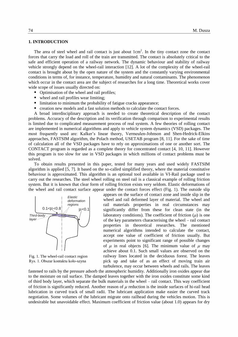
Typical 4-axle passenger vehicle model is employed in the simulations (Fig. 2). Vehicle model

corresponds to the 127A passenger car of Polish rolling stock. Bogies of the vehicle have 25AN

designation in Polish terminology. The model consists of fifteen rigid bodies representing: carbody,

two bogies with two solid wheelsets and eight axleboxes. Each wheelset is attached to axleboxes by

joint attachment of a revolute type. So rotation of the wheelsets around the lateral axis with respect to

axleboxes is only possible. Arm of each axlebox is attached to bogie frame by pin joint (bush type

76 M. Dusza

element). They are laterally, longitudinally and rotary flexible elements. The linear and bi-linear

characteristics of the primary and secondary suspension are included in the model. They represent

metal (screw) springs and hydraulic dampers of primary and secondary suspension. In addition torsion

springs (kbcb) are mounted between car body and bogie frames. To restrict car body – bogie frame

lateral displacements, bumpstops with 0.03 m clearance were applied (not visible in Fig. 2). A new

S1002 wheel and UIC60 rail pairs of profiles are considered. Non-linear geometry of wheel - rail

contact description is assumed. Contact area and other contact parameters are calculated with use of

RSGEO subprogram (implemented into VI-Rail). To calculate wheel-rail contact forces, results

obtained from RSGEO are utilized. In order to calculate tangential contact forces between wheel and

rail, so called non-linear simplified theory of the rolling contact by J.J. Kalker is applied. It is

implemented in the computer code FASTSIM [5, 7] used worldwide.

Fig. 2. Vehicle – track nominal model structure: a) side view, b) front view, c) top view

Rys. 2. Struktura modelu nominalnego pojazd – tor: a) widok z boku, b) widok z przodu, c) widok z góry

2.2. Track Model

Discrete, two level, vertically and laterally flexible track models were assumed (Fig. 3). But

models of track flexibility are simplified. For low frequency analysis (less than 50 Hz) simplified track

model is accepted when dynamics of vehicle motion is considered. Rails and sleepers are treated as a

lumped mass (mr, ms) of the corresponding rigid bodies. No track irregularities are taken into account.

Periodic support of the rails in real track is neglected in the model too. So, the non-inertial type of the

moving load is adopted here. Linear elastic springs and dampers connect the track parts (rigid bodies)

to each other. Similar approach is used in many works in vehicle dynamics where just low frequency

deformations of the track are of the interest, e.g. [3, 4, 8 - 10, 12].

k

x

y

z

rt

k c

z

y

mbc

1z

1z c1z

k1z

ck

kc

m

m

r

s

vrs

vrs

vsgvsg

c2z k

2zmb

pivot

mcb

krt

c

1z

1z c1z

k1z

ck

k c

m

m

r

s

vrs vrs

vsg vsg

c2z k

2zmb

pivot

19 m

26,1 m

1z1z

c1z

ab klrs

klsgkc

k

c

c k

vrs

vrs

vrs

vrsclrs

vsg vsg clsg

mr

ms

c

m

kbcb

k2y

2y

ck

2y

2y

c1y

k1y

k1y

c

k1x

1x

bogieframec

1y

2,5 m

c1y

k1y

k1y

c

k1x

1x

c1y

2,5 m

axlebox

x

2,9

m

2,83 m

mcb

a) b)

c)


The track has got nominal UIC60 rails with a rail inclination 1:40. Each wheelset is supported by a

separate track section consisting of two rail parts and sleepers that correspond to 1m length of typical

ballasted real track. Every wheelset – track subsystem has homogenous properties and is independent

from one another. Each route of curved track model is composed of short section of straight track,

transition curve and regular arc. Constant value of superelevation depending on curve radius value is

applied for each curved track route (Table 1).

Table 1

Curve radii tested and track superelevations corresponding to them

Curve radius R [m] 3000 6000

Superelevation h [m] 0.110 0.051 0

ck

rt

mb

ck

k c

m

m

r

s

vrs vrs

vsg vsg

1z

1z

lrs lrs klsg

kc k c

c k

vrsvrs vrs vrsc clrs lrs

vsg vsg clsg

ms

mr

y

k k

2b

z

14

smoothsurface 1:40

1:40

railinclinationx

a) b)

pinjoint

Fig. 3. Track nominal model structure: a) side view, b) cross section view

Rys. 3. Struktura nominalna modelu toru: a) widok z boku, b) w przekroju poprzecznym

Detailed vehicle and track model parameters are collected in Appendix.

3. THE METHOD

Basically, the method used by the author in the present study is based on the bifurcation approach

to the analysis of rail vehicle lateral stability. This approach is widely used in the rail vehicle lateral

dynamics, e.g. [4, 9, 10, 12 and 1, 2, 13-15]. This method takes account of the stability theory,

however is less formal than the theory but more practical instead. In another word, it also makes use of

some assumptions and expectations from the system being studied, which are based on the already

known general knowledge about the rail vehicle systems. In accordance with that, building the

bifurcation plot is the main objective here but formal check if the solutions on this plot are formally

stable is not such an objective. That is why one does not adopt some solution as the reference one in

this approach and then does not introduce some perturbation into the system to check if the newly

obtained solution stays within some narrow vicinity of the reference solution, what definition of the

stability (theory) would require. The approach assumes that any solution typical for railway vehicle

systems (stationary or periodic) is stable. Such assumption could be accepted based on the

understanding within the railway vehicle dynamics that periodic solutions are the self-exciting

vibrations that are governed by the tangential forces in wheel-rail contact. Thanks to it, the self-

exciting vibrations theory can be used to expect (predict) typical behaviour of the system. Only when

78 M. Dusza

serious doubts about stability appear, formal check for the stability (with the initial conditions

variation to introduce the perturbation) is then performed.

On the other hand, another very important reason exists to vary the initial conditions. This is the

need to get all the solutions in order to build the complete bifurcation diagram. Varying the initial

conditions carefully, widely and knowingly enables to obtain all multiple solutions for the particular

velocity v value. It is the case for both the stable and unstable solutions as well as stationary and

periodic solutions known in the railway vehicle dynamics. Repeating the procedure for all velocity

range makes it possible to get the bifurcation plots, as e.g. Figs. 4a and 4b. As it is seen on these

figures the bifurcation plots represent stability properties of the system as they show precisely areas of

the stable and unstable solutions, both the stationary and periodic ones. The crucial elements on the

plots are saddle-node bifurcation and subcritical Hopf’s bifurcation that correspond to the stable

solutions lines and velocities vn and vc, respectively (see Figs. 4a and 4b). The vn and vc are well

known in the rail vehicle stability analysis non-linear and linear critical velocities, respectively.

It is worth adding that bifurcation approach, focused on building the bifurcation diagrams, is also

suitable to represent less typical behaviours of the railway vehicle systems, as chaotic ones. Then more

formal activities are necessary, however.

Interpretation and extension to the above statements, including physical aspects, can be found in

[14, 15] where thorough considerations are presented, which enable dipper understanding of the rail

vehicle lateral stability analysis. The method presented in [15] is more formal than that in [14].

According with the above the information is given below, referring to the considered objects, on

how the bifurcation plots for the needs of the present paper were built. The first part refers to the

straight track case, while the second one to the circular curve case.

In the method used, the first bogie’s leading wheelset lateral displacements yp are observed and

recorded in time domain (as in Figs. 4c and 4d). The stable stationary solutions can appear (Fig. 4c) in

the system. They are typical for vehicle velocity less than the critical value vn. Sometimes in a curved

track for velocity higher than the critical one they appear as well. In case of the stable stationary

solutions zero lateral displacements and peak-to-peak values in straight track are observed. In addition,

the tested vehicle model is example of hard excitation system, e.g. [14]. It means that some minimum

value of initial conditions have to be imposed to initiate periodic solutions (self-exciting vibrations in

real system). Alternatively, some other perturbation in the system has to be introduced. Thus, in order

to initiate vibrations the straight track test section has got singular lateral irregularity situated 200 m

from the track beginning. The irregularity has half of sine function shape. Its amplitude equals 0.006

m and wave length 20 m. So all wheelsets are shifted in lateral direction in straight track during the

irregularity negotiation. Afterwards the wheelsets tend to central position (for velocity lower than the

critical value vn) or lateral displacements increase and may change periodically (for velocity equal or

bigger then the critical value vn). The smallest motion velocity for which stable periodic solutions

(limit cycles) appear is accepted as a critical value vn. The step of velocity changes equal 0.1 m/s was

applied in particular simulations processes. Hence, the accuracy of critical velocity value

determination is equal to 0.1 m/s, too. Existence of periodic solutions (self-exciting vibrations in real

object) means also energy dissipation in the system. Two conditions have to be met to initiate the

periodic solutions. The first is some minimum value of energy delivered to the system (minimum

velocity value in the tested system). The second is application of some minimum value of initial

excitation (e.g. track irregularity of sufficient amplitude). The periodic solutions (limit cycles) are

generally not desirable in real objects because vibration is always worse than stationary behaviour. On

the other hand limited (and constant) value of the amplitude enables safe vehicle motion.

Consequently, such type of solutions can be accepted as being the stable one. Amplitude as well as

other limit cycle parameters can constitute some indicators of the system state. The maximum of

wheelset lateral displacements (yp max) and their peak-to-peak values (p-t-p yp) are utilized in the

method.

Non-zero lateral displacements (vibrations) appear in the initial part of curved track, usually (as for

R = 2000 m in Fig. 4c). It is caused by the lack of balance between lateral (with respect to track plane)

forces acting on the vehicle in curve. Another word, the lateral components of centrifugal and gravity

forces do not neutralize each other. Stationary value of wheelset lateral displacement becomes


established after enough long time (12 seconds in Fig. 4c). So, stable stationary non-zero solutions

exist in curved track for velocity lower than vn, usually. Exceeding the critical velocity value vn means

self-exciting vibrations appearance. It causes for vehicle model transfer (bifurcation) of solutions from

the stable stationary to the stable periodic ones (Fig. 4d). The wheelsets move periodically along

lateral axis y and rotate round their vertical axis z. It is the form of energy dissipation, typical in

wheelset-track system. Similarly to the straight track case, two conditions should be fulfilled to initiate

the self-exciting vibrations in circular curve too. The first one is some minimum velocity value of

wheelset (vehicle). The second one is sufficiently big initial excitation of the wheelset. For the

analysis of stability in curved track sections it is not sure if the initial excitation at the beginning of

straight track section can play its role sufficiently. On the other hand transition curve negotiation

appeared to be quite enough excitation to initiate periodic solutions in the regular curve (if vehicle

velocity is equal or exceeds the critical value vn). That is why the lateral irregularity in straight track is

not applied in curved track cases.

In practice, to obtain the results for curved track, compound routes had to be applied. It is the

consequence of VI-Rail software feature. It cannot start calculations in a curved track directly.

Therefore simulations, which finish in a curved track, have to begin in straight track section (first 3

seconds in Fig. 4c and 4d). Then they pass through transition curve and finally the regular curved track

section (R = const.) begins. If the wheelset’s lateral motion takes form of limit cycle and exists until

end of the test time (15 s usually), the state represents and is called the stable periodic solution

(Fig. 4d).

Constant value of velocity is taken in each simulation. Two parameters – maximum of leading

wheelset lateral displacement absolute value (|yp|max) and peak-to-peak value of yp (p-t-p yp) are

determined. Diagrams of these parameters in velocity domain (Fig. 4a and 4b) are created. Both

graphs include the lines matching circular track sections of radii from R = 1200 m to R = (straight

track). So a few lines are presented in the complete diagrams usually. Each line is created following a

series of single simulations for different v and the same route. The range of v starts at low velocities,

passes critical value vn and terminates in velocities vd, called sometimes the derailment velocity. The

value vd does not mean the real derailment, however. This is the lowest value of velocity for which

results of simulations take no limit cycle shape and no quasi-static shape either. But the vehicle motion

is possible often. In addition, if wheelset lateral displacements take large values the climb of wheels on

rail head could happen. In curved track, outer wheel may be lift up and can loss contact at velocity vd

sometimes. It is effect of centrifugal force acting and it is treated as a derailment too. The pairs of

diagrams like those visible in Figure 4a and 4b, which include results for all tested curve radii, are

called a ,,stability maps” and selected as a form of results presentation.

The meaning of stable motion of vehicle in the current research should be expressed here, now.

Just stable stationary solutions (constant value of wheelset lateral displacement yp) or stable periodic

solutions (limit cycle of yp) are assumed to describe stable vehicle motion. Any other solutions are

assumed to be the unstable ones. The periodic motion of wheelset corresponding to its limit cycle is

not desirable in real vehicle exploitation of course. On the other hand, limit cycle in the stability

analysis means constant peak-to-peak value and frequency of the wheelset lateral displacements.

Consequently, if the maximum of wheelset lateral displacement value does not exceed the permissible

value, vehicle motion is possible and to some extent safe.

Great practical significance has the non-linear critical velocity vn. It is a good idea to take it at least

a bit higher than velocity permissible for real object (maximum service speed of the vehicle). Stable

solutions exist in range of velocity smaller and bigger than the critical value vn. But distance between

the critical value vn and the derailment value vd can be significantly different in individual tests. This

distance depends on the vehicle – track system parameters (see results). From the practical point of

view the critical velocity should be high and distance between critical velocity and derailment velocity

possibly long.

80 M. Dusza

Fig. 4. Scheme of creating the pair of bifurcation plots useful in the curved track analysis

Rys. 4. Schemat metody tworzenia par wykresów bifurkacyjnych w badaniach ruchu po łuku

4. THE RESULTS

Considering the coefficient of friction () influence on rail vehicle model stability, straight track

motion was analysed at the beginning. The results are presented in Figure 5. Constant velocity value is

applied in each simulation. Just stable stationary solutions exist for velocities lower than 40m/s (yp = 0

and p-t-p yp = 0). So, the results for velocity bigger than 40m/s are presented. For eight values of

increased from 0.1 to 0.8 (with the step 0.1), series of simulations were executed. The velocity of

motion is increased in the next simulation (executed for particular value) with the step 2m/s. But in

case of sudden change of solution value or of solution character the velocity step was dropped to

0.1m/s.

The smallest critical velocity value vn = 58m/s appears for = 0.1. The smallest |yp|max and p-t-p

yp exist in this case in comparison to results for bigger values. The |yp|max achieves about 0.0067m

and p-t-p yp about 0.0134m. Both these parameters increase at the beginning and over the range of

critical velocities and then stabilize. Although no derailment indicatives appear the simulations were

discontinued at 200m/s. Velocities bigger than 200m/s (720km/h) are too unrealistic to apply in real

systems yet. Critical velocity increases to 62m/s for = 0.2. Both the observed parameters increase in

the initial range and over critical velocities and then stabilize. But values of these parameters are

bigger at the same velocity in comparison with the previous case. The series of simulations was

stopped at 200m/s in this case too. Next was increased to 0.3. The critical velocity value appears at

63.3m/s. It was the biggest critical velocity value in the straight track case. Gentle increase of |yp|max

and p-t-p yp is observed in the initial range over the critical velocity values. Then both parameters

50 70 90 110

vehicle velocity; [m/s]

0.000

0.001

0.002

0.003

0.004

0.005

0.006

peak-t

o-p

eak

valu

eo

fy

p;

[m] Stable periodic solutions

R=2000m

b)

Stablestationarysolutions

vn vc vd

Unstablesolutionsperiodic,stationary

50 70 90 110

vehicle velocity; [m/s]

0.000

0.001

0.002

0.003

0.004

0.005

0.006

0.007

0.008

max

imu

mo

fle

ad

ing

wh

eels

et

late

ral

dis

pla

cem

en

ta

bso

lute

va

lue

|yp|m

ax;

[m]

Stable periodicsolutions

R=2000m

a)

Stablestationarysolutions

vn vcvd

Unstablestationarysolutions

Unstable periodicsolutions

0 2 4 6 8 10 12 14t; [s]

-0.006

-0.004

-0.002

0

0.002

0.004

yp;

[m]

d)

R=2000m

v=75m/s > vn

Straight track

Transition curve

Regular arcR=2000m

0 2 4 6 8 10 12 14

t; [s]

-0.006

-0.004

-0.002

0.000

0.002

0.004

yp;

[m]

v=65m/s < vn

R=2000m

c)

Straight track

Transition curve

Regular arcR=2000m


increase significantly in the velocity range 100 … 140m/s and stabilize for velocity bigger than

160m/s. Simulations were stopped at 200m/s in this case too. The critical velocity value vn = 61.8m/s

appears for = 0.4. Both observed parameters increase in the initial range over the critical velocity

values and stabilize for velocities bigger than 100m/s. 129m/s is the maximum velocity value for

which stable solutions exist. The |yp|max achieve about 0.0095m and p-t-p yp about 0.0190m at this

velocity. Thus significant cut of the velocity range of stable solutions can be observed.

40 80 120 160 200

v; [m/s]

0.000

0.002

0.004

0.006

0.008

0.010

|yp|m

ax; [m

]

vn=58 ... 63,3 m/s

Straight track UIC60/S1002

40 80 120 160 200

v; [m/s]

0.000

0.004

0.008

0.012

0.016

0.020

pe

ak-t

o-p

ea

k v

alu

e o

f y

p;

[m] Straight track

UIC60/S1002

vn=58 ... 63,3 m/s

Fig. 5. Maximum of absolute value of leading wheelset lateral displacements (|yp|max) and peak-to-peak value of

the leading wheelset lateral displacements versus velocity of motion along straight track for wheel-rail

coefficients of friction from 0.1 to 0.8

Rys. 5. Wartości maksymalne z bezwzględnych wartości przemieszczeń poprzecznych pierwszego zestawu koło-

wego (|yp|max) oraz wartości międzyszczytowe tych przemieszczeń (peak-to-peak value of yp) w funkcji

prędkości ruchu na torze prostym dla współczynników tarcia koła – szyny od 0,1 do 0,8

The same critical velocity value 61.8m/s appears for = 0.5. The maximum velocity of stable

solutions existence is equal 98m/s. Critical velocity slightly increase to 62.8m/s for = 0.6. But the

maximum velocity of stable solutions decreases to 89m/s. |yp|max = 0.0094m and p-t-p yp = 0.0188m

at this velocity. Critical velocity value vn = 61m/s for the biggest values 0.7 and 0.8. Maximum

velocity values for which stable solutions exist are equal 78m/s and 75m/s for = 0.7 and 0.8,

respectively. Thus the ranges over the critical velocity of stable solutions are short in comparison to

these for smaller values.

Similar range of simulations for curved track motion was executed. Big curve radius R = 6000m

was applied at the beginning. The results are presented in Fig. 6. Stable stationary solutions exist for

velocity smaller than 40m/s (similarly to straight track case). It means that p-t-p yp = 0 but yp 0. It is

an effect of balance lack between lateral forces acting on vehicle while curve track negotiating.

Wheelset lateral displacements decrease from about 0.0015m to 0.0012m in velocity range 40

…62m/s. The smallest critical velocity value 62m/s appear for = 0.1. The yp increases to 0.0057m in

the initial range over the critical velocity and then decreases to about 0.001m at velocity 95m/s.

Bifurcation of solutions appears at this velocity value. Stable periodic solutions disappear, p-t-p yp = 0

and |yp|max rises from 0.001m to 0.0043m. Stable stationary solutions exist for velocities bigger than

95m/s. Increase of |yp|max to 0.0061m can be observed and 140m/s is the maximum velocity value for

which stable solution exists. The critical velocity increased to 66.7m/s for bigger = 0.2. Increase of

p-t-p yp and |yp|max for analogous velocities in comparison to previous case (for = 0.1) can be

observed. Both observed parameters increase in the range of velocity from critical value to about

96m/s. Then they decrease and bifurcation point appears at velocity 115m/s. The p-t-p yp drops to zero

and |yp|max increases from about 0.001m to 0.002m. Stable stationary solutions exist above velocity

115m/s. The |yp|max increases to about 0.0061m at 142m/s and this is the maximum velocity for which

82 M. Dusza

stable solution exists. Coefficient of friction = 0.3 was applied next. The critical velocity vn =

69.5m/s. Both of observed parameters achieve maximum, |yp|max = 0.0075m and p-t-p yp = 0.0144m,

at velocity 105m/s. Then they decrease and bifurcation point appears at velocity 126m/s.

40 60 80 100 120 140

v; [m/s]

0.000

0.002

0.004

0.006

0.008

0.010

|yp|m

ax; [m

]

vn=62 ... 74 m/s

UIC60/S1002

R=6000m

40 60 80 100 120 140

v; [m/s]

0.000

0.004

0.008

0.012

0.016

0.020

pe

ak-t

o-p

ea

k v

alu

e o

f y

p;

[m]

UIC60/S1002

vn=

62

m/s

R=6000m

vn=

74

m/s


the leading wheelset lateral displacements versus velocity of motion along curved track of radius R =

6000m for wheel-rail coefficients of friction from 0.1 to 0.8

Rys. 6. Wartości maksymalne z bezwzględnych wartości przemieszczeń poprzecznych pierwszego zestawu

kołowego (|yp|max) oraz wartości międzyszczytowe tych przemieszczeń (peak-to-peak value of yp)

w funkcji prędkości ruchu na torze o promieniu łuku R = 6000m dla współczynników tarcia koła –

szyny od 0,1 do 0,8

Stable stationary solutions exist for velocities up to 140m/s. The critical velocity decreases to

63m/s for = 0.4. The observed parameters achieve maximum |yp|max = 0.0078m and p-t-p yp =

0.0157m in the range of velocity 100 … 110m/s. Next they decrease and bifurcation point appears at

133m/s. Stable stationary solutions exist until 142m/s. Increase of critical velocity to 70.7 m/s is

observed for = 0.5. Maximum of the observed parameters appears in the range of velocity 95

…105m/s, |yp|max = 0.0085m and p-t-p yp = 0.0165m. Stable periodic solutions exist in the range of

velocities up to 134m/s. The applied = 0.5 is the minimum value for which stable periodic

solutions exist in whole over critical range of velocity (lack of bifurcation points). Critical velocity

value vn = 74m/s for coefficient of friction = 0.6 appears. It is the biggest vn value among the eight

cases tested. |yp|max increase from 0.0077m at critical velocity to 0.0098m at 95m/s (the maximum

velocity for which stable solutions exists). The p-t-p yp increase from 0.0152m to 0.019m in the same

velocity range. So, significant decrease of the velocity range (in comparison with the smallest value

cases) for which stable solutions exist can be observed. The critical velocities achieve 66.5m/s and

65.6m/s for the biggest values tested, 0.7 and 0.8 respectively. Both observed parameters increase

and achieve |yp|max = 0.0098m and p-t-p yp = 0.0182m at the maximum velocities for which stable

solutions exist, i.e. 90 and 92m/s respectively.

Curved track motion for smaller curve radius R = 3000m was analysed next. The results are

presented in Figure 7. The smallest value 0.1 was applied at the beginning. Stable stationary

solutions exist for velocities up to 55.4m/s. The |yp|max achieves about 0.003m and p-t-p yp = 0 for

smaller velocities. At the critical velocity vn = 55.4m/s periodic solutions appear. Both observed

parameters increase to |yp|max = 0.0047m and p-t-p yp = 0.0058m at velocity about 64m/s. Then both

parameters decrease to 0.0016m and 0.001m, respectively and bifurcation point appears at velocity

76m/s. Stable stationary solutions exist up to 112m/s. |yp|max increases from 0.0046m to 0.0061m.

The critical velocity increases to 58m/s for = 0.2. Maximum of both observed parameters fall at

velocity about 74m/s. The |yp|max = 0.0059m and p-t-p yp = 0.0098m. Then both parameters decreases


and bifurcation point appears at velocity 86m/s. Stable stationary solutions exist up to 106m/s. The

critical velocity increases to 66.6m/s for increased to 0.3. Similarly to previous cases both observed

parameters rise in the initial range over the critical velocity values and the maximum is achieved at

about 76m/s, |yp|max = 0.0066m and p-t-p yp = 0.0124m.

40 60 80 100 120 140

v; [m/s]

0.000

0.002

0.004

0.006

0.008

0.010

|yp|m

ax;

[m]

vn=55,4 ... 72 m/s

UIC60/S1002

R=3000m

40 60 80 100 120 140

v; [m/s]

0.000

0.004

0.008

0.012

0.016

0.020

pe

ak-t

o-p

ea

k v

alu

e o

f y

p;

[m]

UIC60/S1002

R=3000m

vn=55,4 ... 72m/s


the leading wheelset lateral displacements versus velocity of motion along curved track of radius R =

3000m for wheel-rail coefficients of friction from 0.1 to 0.8

Rys. 7. Wartości maksymalne z bezwzględnych wartości przemieszczeń poprzecznych pierwszego zestawu

kołowego (|yp|max) oraz wartości międzyszczytowe tych przemieszczeń (peak-to-peak value of yp)

w funkcji prędkości ruchu na torze o promieniu łuku R = 3000m dla współczynników tarcia koła –

szyny od 0,1 do 0,8

Then both parameters decrease and bifurcation of solutions appears at 90m/s. Stable stationary

solutions exist for velocity rising up to 108m/s. Critical velocity value increases to 70.9m/s for = 0.5.

The solution slightly increases at the beginning range over the critical velocities. Then it decreases and

bifurcation point appears at velocity 98m/s. Stable stationary solutions exist for velocities up to

108m/s. The biggest critical velocity value 72m/s appears for = 0.6. Periodic solutions exist up to

96m/s. No bifurcation points are observed for this and bigger values in the range over the critical

velocity. The critical velocity values achieve 69.8 and 70.5m/s for the biggest values, 0.7 and 0.8

respectively. Stable periodic solutions exist up to 98 and 96m/s in these cases. Both observed

parameters achieve maximum values here in comparison to the smallest values cases.

5. CONCLUSIONS

Significant influence of wheel-rail coefficient of friction on rail vehicle stability can be observed.

Increase of from 0.3 to 0.5 means significant decrease of the range of velocities for which stable

solutions exists in the case of straight track motion. From theoretical point of view, stable motion at

velocity of 100m/s with = 0.3 is possible. Increase of to 0.5 (or more) makes the motion unstable

(derailment of vehicle). Increase of wheelset lateral displacements yp according to increase can be

observed too. It is not desirable effect also. But the influence on critical velocity value is slight

(in the range of 5.3m/s). Some different features in curved track can be observed. The range of vn

changes for different values achieves 12m/s for R = 6000m. The range increases to 16.6m/s for

smaller R = 3000m. So increasing influence on vn can be observed while R decreases. No regularity

of vn dependence on value can be observed. The vn achieves minimum for = 0.1 and maximum for

= 0.6 usually. Bifurcation of solutions from stable periodic to stable stationary for velocities bigger

than the critical value does not constitute the emergency of derailment in the real system.

84 M. Dusza

References

1. Dusza, M. & Zboiński, K. Bifurcation approach to the stability analysis of rail vehicle models

in a curved track. The Archives of Transport. 2009. Volume XXI. No. 1-2. P. 147-160.

2. Dusza, M. The study of track gauge influence on lateral stability of 4-axle rail vehicle model. The

Archives of Transport. 2014. Volume XXX. No. 2. P. 7-20.

3. HyunWook Lee & Corina Sandu Carvel Holton Dynamic model for the wheel-rail contact friction.

Vehicle System Dynamics. 2012. Vol. 50. No. 2. P. 299-321.

4. Iwnicki, S. (editor). Handbook of Railway Vehicle Dynamics. London, New York: Taylor &

Francis Group. LLC. 2006.

5. Kalker, J.J. A fast algorithm for the simplified theory of rolling contact. Vehicle System Dynamics.

1982. Vol. 11. P. 1-13.

6. Olofsson, U. & Zhu, Y. & Abbasi, S. & Lewis, R. & Lewis, S. Tribology of the wheel-rail contact

– aspects of wear, particle emission and adhesion. Vehicle System Dynamics. 2013. Vol. 51. No. 7.

P. 1091-1120.

7. Piotrowski, J. Kalker’s algorithm Fastsim solves tangential contact problems with slip-dependent

friction and friction anisotropy. Vehicle System Dynamics. 2010. Vol. 48. No 7. P. 869-889.

8. Polach, O. Characteristic parameters of nonlinear wheel/rail contact geometry. Vehicle System

Dynamics. 2010. Vol. 48. Supplement. P. 19-36.

9. Schupp, G. Computational Bifurcation Analysis of Mechanical Systems with Applications to Rail

Vehicles. Vehicle System Dynamics. 2004. Vol. 41. Supplement. P. 458-467.

10. Shabana, A.A. & Zaazaa, K.E. & Sugiyama, H. Railroad Vehicle Dynamics a Computational

Approach. London, New York: Taylor & Francis Group. LLC. 2008.

11. Vollebregt, E.A.H. & Iwnicki, S.D. & Xie G. & Shackleton, P. Assessing the accuracy of different

simplified frictional rolling contact algorithms. Vehicle System Dynamics. 2012. Vol. 50. No. 1.

P. 1-17.

12. Wilson, N. & Wu, H. & Tournay, H. & Urban, C. Effects of wheel/rail contact patterns and

vehicle parameters on lateral stability. Vehicle System Dynamics. 2010. Vol. 48. Supplement.

P. 487-503. In: 21st International Symposium IAVSD. Stockholm, Sweden. 2009.

13. Zboiński, K. & Dusza, M. Development of the method and analysis for non-linear lateral stability

of railway vehicles in a curved track. Vehicle System Dynamics. 2006. Vol. 44. Supplement.

P. 147-157. In: Proceedings of 19th IAVSD Symposium. Milan. 2005.

14. Zboiński, K. & Dusza, M. Self-exciting vibrations and Hopf’s bifurcation in non-linear stability

analysis of rail vehicles in curved track. European Journal of Mechanics. Part A/Solids. 2010.

Vol. 29. No. 2. P. 190-203.

15. Zboiński, K. & Dusza, M. Extended study of rail vehicle lateral stability in a curved track. Vehicle

System Dynamics. 2011. Vol. 49. No. 5. P. 789-810.

Appendix

Table A1

Mass parameters

Variable Description Unit Value

mcb Car body mass kg 32 000

mb Bogie frame

mass kg 2 600

mw Wheelset mass kg 1 800

mab Axle box mass kg 100

mr Rail mass kg 60

ms Sleeper mass kg 500


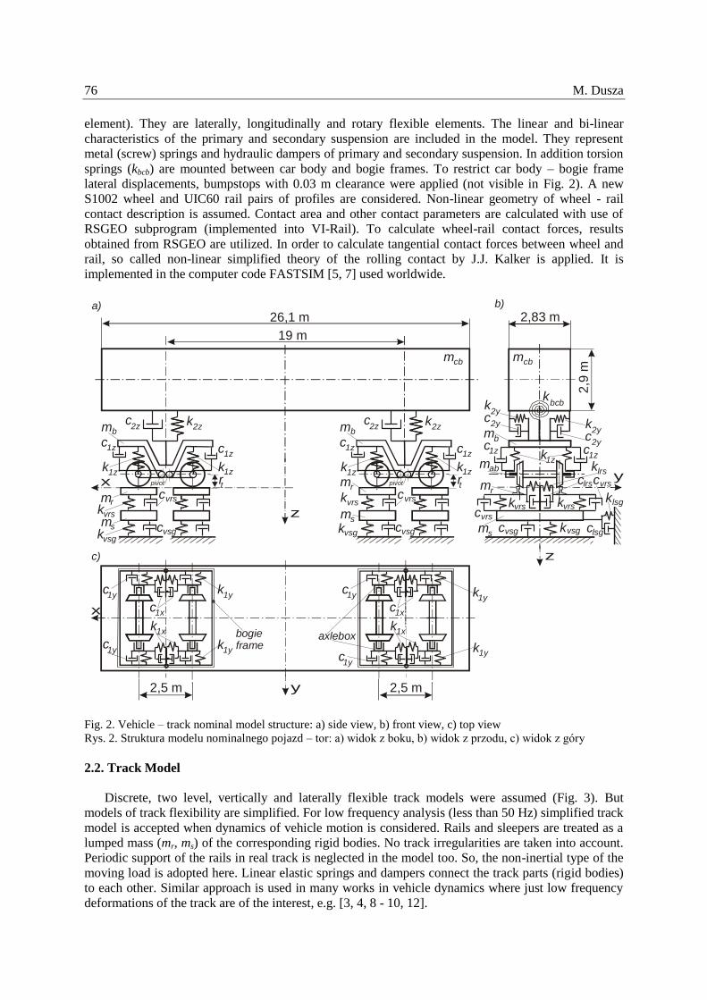
Table A2

Vehicle model suspension parameters

Variable Description Unit Value Comment

k1x Longitudinal primary

suspension stiffness N/m 30 000 000

k1y Lateral primary suspension

stiffness N/m 50 000 000

k1z Vertical primary suspension

stiffness N/m 732 000

Preload force

46 500 N

c1x Longitudinal primary

suspension damping Ns/m 0

c1y Lateral primary suspension

damping Ns/m 0

c1z Vertical primary suspension

damping Ns/m

Linear damping 7 000

Series stiffness 600

000

Nonlinear

with series

stiffness

k2x Longitudinal secondary


k2y Lateral secondary


k2z Vertical secondary


Preload force

80 000 N

c2x Longitudinal secondary

suspension damping Ns/m 0

c2y Lateral secondary

suspension damping Ns/m

Linear damping 1

Series stiffness 6 000

000

Nonlinear

with series

stiffness

c2z Vertical secondary

suspension damping Ns/m

Linear damping 20

000

Series stiffness 6 000

000

Nonlinear

with series

stiffness

kbcb Bogie frame – car body

secondary roll stiffness Nm/rad 16 406

Torsion

spring

Table A3

Track model parameters


kvrs Rail – sleeper vertical stiffness N/m 50 000 000

klrs Rail – sleeper lateral stiffness N/m 43 000 000

cvrs Rail – sleeper vertical damping Ns/m 200 000

clrs Rail – sleeper lateral damping Ns/m 240 000

krrs Rail – sleeper rolling stiffness N/rad 10 000 000

crrs Rail – sleeper rolling damping Ns/rad 10 000

kvsg Sleeper – ground vertical stiffness N/m 1 000 000 000

klsg Sleeper – ground lateral stiffness N/m 37 000 000

cvsg Sleeper – ground vertical damping Ns/m 1 000 000

clsg Sleeper – ground lateral damping Ns/m 240 000

krsg Sleeper – ground rolling stiffness Nm/rad 10 000 000

crsg Sleeper – ground rolling damping Nms/rad 10 000

86 M. Dusza

Table A4

Inertia parameters


icbxx

Car body inertia

kgm2 56 800

icbyy kgm2 1 970 000

icbzz kgm2 1 970 000

ibfxx Bogie frame

inertia

kgm2 1 722

ibfyy kgm2 1 476

ibfzz kgm2 3 067

iwxx

Wheelset inertia

kgm2 1 120

iwyy kgm2 112

iwzz kgm2 1 120

iaxx

Axlebox inertia

kgm2 20

iayy kgm2 12

iazz kgm2 20

Table A5

Outside dimensions


lcb

Car body

length m 26.1

wcb width m 2.83

hcb height m 2.9

lbf Bogie

frame

length m 3.06

wbf width m 2.16

hbf height m 0.84

2a

Wheelset

wheelbase m 2.5

2c axle length m 2.0

2b

rolling

circles

distance

m 1.5

rt radius m 0.46

Parameters Arrangement in Simulations:

The VI-Rail software enables users to arrange and adjust many of the computational parameters. The

simulation specification, selected method of mathematical description of real elements, and equation

solver procedure choice have significant influence on the final results. List of the parameters applied

in each simulation is presented below.

Simulation time – 15 s;

Number of Steps – 2500;

Contact Configuration File – mdi_contact_tab.ccf;

Track Type – flexible; Wheel – rail coefficient of friction (variable) – 0.1 … 0.8;

Young Modulus – 2.1E+11;

Poisson’s Ratio – 0.27;

Cant Mode – Low Rail;

Solver Selection – F77;

Solver Dynamics Setting: Integrator – GSTIFF, Formulation – I3.

Received 23.11.2013; accepted in revised form 19.08.2015

Documents

THE WHEEL-RAIL CONTACT FRICTION INFLUENCE · PDF file74 M. Dusza Third-body layer Elastic deformation regions 0.1