The welfare effects of a partial tariff reduction under

The welfare effects of a partial tariff reduction under domestic distortion in

Japan

by

Akihito Asano and

Michiru S Kosaka

ANU Working Papers in Economics and Econometrics # 650

May 2017 JEL: F11, F13

ISBN: 0 86831 650 4

The welfare effects of a partial tariff reduction under

domestic distortion in Japan∗

Akihito Asano†

Sophia University

Michiru S Kosaka‡

Sophia University

May 1, 2017

Abstract

We examine a partial tariff reduction policy in a specific factor model with two

import-competing sectors. When one of them enjoys a higher tariff and is also

subject to a production subsidy, will a tariff reduction in the other import-competing

sector be welfare improving? We argue that this second-best type question is highly

relevant to Japan, and calibrate our model to its 2013 economy. We find that the

policy is undesirable and that even a complete subsidy removal is insufficient to

make it desirable. Making it welfare improving requires the other sector’s tariff be

more than halved.

Keywords: Tariff policy, domestic distortion, welfare, specific factor model, Japanese

economy

JEL Classification: F11(Neoclassical Models of Trade), F13(Trade Policy; International

Trade Organizations)

∗The authors would like to thank participants of Economic Theory Seminar at the Australian Na-tional University for feedback, and in particular, Taiji Furusawa and Martin Richardson for their helpfulcomments and suggestions. This paper was completed when Asano was visiting the Australian NationalUniversity, and he thanks the Research School of Economics for their hospitality. The usual disclaimerapplies.

†Corresponding author. E-mail: [email protected].‡E-mail: [email protected].

1

1 Introduction

Japan is one of the world’s largest agro-food importing countries and it is well known

that significant support has been provided to its producers. According to OECD (2017),

the producer support estimates (PSE) for Japanese farmers in 2013 was 52 per cent

of gross farm receipts, which was well beyond the PSE in most other OECD countries

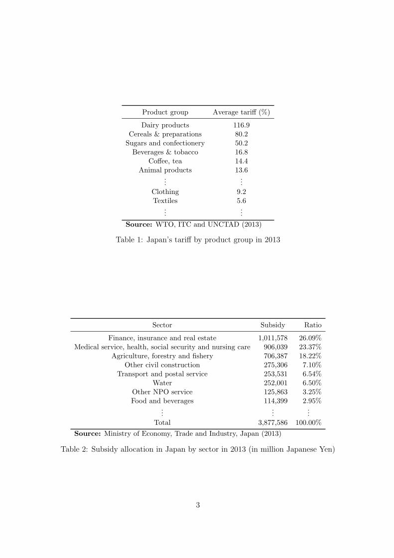
(see Figure 1). Indeed, Table 1 indicates that high average tariff rates were imposed

on Japanese agricultural imports such as Dairy products (116.9 per cent), Cereals and

preparations (80.2 per cent), and Sugars and confectionery (50.2 per cent).

0

10

20

30

40

50

60

70

80

1985 1990 1995 2000 2005 2010 2015

Japan

Korea

Australia

United States

European Union

Pro

duce

r support

estim

ate

s

Year

Figure 1: Producer support estimates (% of gross farm receipts, 2013). Source: OECD(2017)

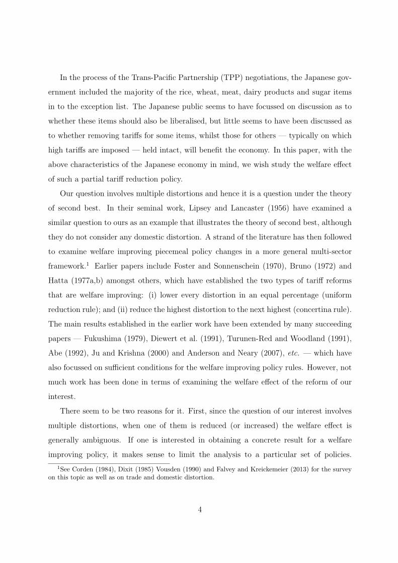
Agricultural producer support in Japan is distinctive also in terms of the government

subsidy. Table 2 suggests that the government subsidy allocated to the ‘Agriculture,

forestry and fishery’ sector is the third largest after ‘Finance, insurance and real estate’

and ‘Medical service, health, social security and nursing care’ sectors. Amongst primary

and manufacturing sectors, the subsidy allocated to the ‘Agriculture, forestry and fishery’

sector exceeds 80 per cent of the total subsidy. On the contrary, protection for other

import-competing sectors — e.g. ‘Textile products’ and ‘Wearing apparel and other textile

products’ — have been rather modest in terms of both import tariffs and subsidies.

2

Product group Average tariff (%)

Dairy products 116.9Cereals & preparations 80.2Sugars and confectionery 50.2Beverages & tobacco 16.8

Coffee, tea 14.4Animal products 13.6

......

Clothing 9.2Textiles 5.6

......

Source: WTO, ITC and UNCTAD (2013)

Table 1: Japan’s tariff by product group in 2013

Sector Subsidy Ratio

Finance, insurance and real estate 1,011,578 26.09%Medical service, health, social security and nursing care 906,039 23.37%

Agriculture, forestry and fishery 706,387 18.22%Other civil construction 275,306 7.10%

Transport and postal service 253,531 6.54%Water 252,001 6.50%

Other NPO service 125,863 3.25%Food and beverages 114,399 2.95%

......

...Total 3,877,586 100.00%

Source: Ministry of Economy, Trade and Industry, Japan (2013)

Table 2: Subsidy allocation in Japan by sector in 2013 (in million Japanese Yen)

3

In the process of the Trans-Pacific Partnership (TPP) negotiations, the Japanese gov-

ernment included the majority of the rice, wheat, meat, dairy products and sugar items

in to the exception list. The Japanese public seems to have focussed on discussion as to

whether these items should also be liberalised, but little seems to have been discussed as

to whether removing tariffs for some items, whilst those for others — typically on which

high tariffs are imposed — held intact, will benefit the economy. In this paper, with the

above characteristics of the Japanese economy in mind, we wish study the welfare effect

of such a partial tariff reduction policy.

Our question involves multiple distortions and hence it is a question under the theory

of second best. In their seminal work, Lipsey and Lancaster (1956) have examined a

similar question to ours as an example that illustrates the theory of second best, although

they do not consider any domestic distortion. A strand of the literature has then followed

to examine welfare improving piecemeal policy changes in a more general multi-sector

framework.1 Earlier papers include Foster and Sonnenschein (1970), Bruno (1972) and

Hatta (1977a,b) amongst others, which have established the two types of tariff reforms

that are welfare improving: (i) lower every distortion in an equal percentage (uniform

reduction rule); and (ii) reduce the highest distortion to the next highest (concertina rule).

The main results established in the earlier work have been extended by many succeeding

papers — Fukushima (1979), Diewert et al. (1991), Turunen-Red and Woodland (1991),

Abe (1992), Ju and Krishna (2000) and Anderson and Neary (2007), etc. — which have

also focussed on sufficient conditions for the welfare improving policy rules. However, not

much work has been done in terms of examining the welfare effect of the reform of our

interest.

There seem to be two reasons for it. First, since the question of our interest involves

multiple distortions, when one of them is reduced (or increased) the welfare effect is

generally ambiguous. If one is interested in obtaining a concrete result for a welfare

improving policy, it makes sense to limit the analysis to a particular set of policies.

1See Corden (1984), Dixit (1985) Vousden (1990) and Falvey and Kreickemeier (2013) for the surveyon this topic as well as on trade and domestic distortion.

4

Second, once a distortion is added to any framework, the mathematical analysis in general

becomes extremely complicated than otherwise, even in a standard two-sector model.2

It is no surprise that classical work that has examined the relationship between trade

and domestic distortion relies on graphical analysis (Bhagwati and Ramaswami, 1963;

Bhagwati, 1967, for example).

To examine the tariff reform of our interest, we employ a specific factor model (Jones,

1971b; Mussa, 1974) that comprises two import-competing sectors (call them Sectors

A and B) and an export sector (call it Sector C). Both import-competing sectors are

protected by tariffs but only one of them (Sector A, namely Agriculture) is supported by

a production subsidy. Our particular interest is the welfare effect of lowering the Sector

B tariff when it is lower than the Sector A tariff. In this case, as has been established in

the existing literature the welfare effect is ambiguous, and hence we resort to numerical

simulations to understand how the welfare effect of the policy reform of our interest

might be affected by consumer preferences and/or production parameters. We employ

the specific factor model because (i) the parsimonious nature of the model helps interpret

our numerical results clearly; and (ii) we are interested in examining the short-run static

effect of a piecemeal tariff reform on resource allocation.

In our numerical simulations we show that there is a following case. A tariff reduction

in Sector B lowers economies welfare, but if the Sector A subsidy is sufficiently reduced

at the same time, the tariff reduction becomes welfare improving. Given the high tariffs

and heavy subsidies in Sector A described previously, it is interesting to investigate if this

situation applies to the current Japanese economy. To this end, we calibrate our model

to the 2013 Japanese economy using various data. Our calibration result indicates that

Sector B’s tariff reduction lowers economy’s welfare and the direction of the effect does

not change even if the Sector A subsidy is reduced to zero. From the viewpoint of static

2For example, Johnson (1966) employs a numerical approach to sketch the production possibilityfrontier for the 2-by-2 model with a domestic distortion. Jones (1971a) provides mathematical explanationon the concavity of the production possibility frontier under the same situation, although complicatedexpressions make it difficult for us to interpret the results intuitively. Ohyama (1972) provides somemathematical analysis of tariff policies under domestic distortion, but it relies on an ad hoc way ofmodelling the distortion.

5

resource allocation, our result suggests that the partial tariff removal policy of our focus is

undesirable and that it should be accompanied by a significant tariff reduction in Sector

A.

Given the calibrated parameters, we also show that the main driving force of the (neg-

ative) welfare effect of this partial tariff removal policy is an efficiency loss in production.

By lowering the protection in Sector B, more production resource is drawn in to Sector A,

which already have had too much resource allocated in the first place. Further production

inefficiency created by this policy explains roughly 70 per cent of the overall (negative)

welfare effect, whilst the remaining effect can be attributed to an incremental efficiency

loss in consumption.

In the following section, we start with the analysis of a two-sector specific factor model

that incorporates domestic distortion, which helps understand the effect of a tariff policy

under domestic distortion intuitively. In Section 3, we extend our model to three sectors

by adding another import-competing sector. We first show that the concertina type tariff

reform will increase welfare in our specific factor model setup. Then we conduct numeri-

cal simulations to examine how different consumer preferences or production parameters

affect the welfare effect of the tariff reform of our interest. In Section 4, we calibrate our

model to the Japanese economy and present the results. Section 5 concludes.

2 The two-sector model with a domestic distortion

2.1 The setup

We consider a two-sector specific factor model in a small open economy setting. We assume

two goods, Good A and Good C. These goods are produced in two sectors, Sector A and

Sector C, respectively. Outputs are denoted as YA and YC , respectively. International

prices of the two goods are denoted as PA and PC .

There are two production factors. Labour is mobile across the two sectors, LA and

LC . Capital in Sector A, KA, and that in Sector C, KC , are specific factors. We assume

6

Cobb-Douglas production technology for both sectors. More specifically,

YA = LαAK

1−αA , (1)

YC = LγCK

1−γC , (2)

where 0 < α < 1 and 0 < γ < 1. The aggregate quantity of labour in the economy is

given as L, and hence:

L = LA + LC . (3)

We assume that Sector A is an import-competing sector, which is subject to an ad

valorem tariff, τA ≥ 0, and also whose production is subsidised by the government. More

specifically, the Sector A producer receives PA(1 + τA) + sA per unit of production,

where sA is the subsidy per unit of production. Sector C is an export sector.3

The profit functions of each sector are:

πA = PA(1 + τA) + sAYA − wLA − rAKA,

πC = PCYC − wLC − rCKC ,

where w, rA, and rC are the wage and the rental prices of capital in each sector, re-

spectively. Solving the profit maximisation problems, we obtain the following first-order

3sA < 0 corresponds to the case when the Good A production is taxed. Although our interest is thecase where sA > 0, we do not impose any condition on its sign as it has an important implication on ourdiscussion in the next section.

7

conditions.4

w = PA(1 + τA) + sAαLα−1A K1−α

A , (4)

w = PCγLγ−1C K1−γ

C , (5)

rA = PA(1 + τA) + sA(1− α)LαAK

−αA , (6)

rC = PC(1− γ)LγCK

−γC . (7)

The consumer’s utility stems from consumption of the two goods, denoted by QA and

QC . We assume a standard Cobb-Douglas utility function as:

U(QA, QC) = QνAQ

1−νC , (8)

where 0 < ν < 1. Then the consumer’s utility maximisation requires:

QA

QC

=ν

1− ν

PC

PA(1 + τA). (9)

The consumer’s budget constraint is given as:

PA(1 + τA)QA + PCQC = wLA + wLC + rAKA + rCKC − T, (10)

where T is a lump-sum tax, which is the difference between the value of Sector A subsidy

and the tariff revenue. That relationship is equivalent to the government budget constraint

which is given as:

T = sAYA − τAPA(QA − YA). (11)

(1), (2), (4)-(7), (10), and (11) boil down to the balance-of-payment constraint, which is:

PAMA = PCXC , (12)

4Throughout this paper we omit the second-order sufficient conditions for brevity as all our setups arestandard and they are trivially satisfied.

8

where MA and XC are defined as:

MA ≡ QA − YA, (13)

XC ≡ YC −QC . (14)

The equilibrium of the model is characterised by the following equations: (1)-(9) and

(12)-(14).

2.2 Welfare effects of a tariff policy

Let us examine the welfare effects of an increase in the import tariff, τA.5 Partially

differentiating U(QA, QC) in (8) with respect to τA, we get:

∂U

∂τA= ν

(QA

QC

)ν−1∂QA

∂τA+ (1− ν)

(QA

QC

)ν∂QC

∂τA

= ν

ν

ν − 1

PC

PA(1 + τA)

ν−1∂QA

∂τA+ (1− ν)

ν

1− ν

PC

PA(1 + τA)

ν∂QC

∂τA. (15)

The second equality follows from (9). The close examination of various terms leads to the

following proposition.

Proposition 1. In the two-sector model, an increase in the import tariff reduces welfare

for any (non-negative) level of government subsidy.

Proof. We show that ∂U∂τA

< 0 for any sA ≥ 0 in Appendix B.

There is a simple intuition behind this result. Initially, the economy is distorted by

the two policies: the import tariff, τA, and the government subsidy, sA. Both policies

distort production by encouraging labour to be allocated in Sector A than otherwise,

where the former also distorts consumption by affecting the consumer relative price. A

further increase in the import tariff works to distort both production and consumption

5Although our focus is the welfare effect of a reduction in a tariff, in the most of the text we will discussthe opposite, i.e. the welfare effect of an increase in a tariff. Focussing on the latter is less confusing asit is what the (partial) derivative of the maximised utility with respect to a tariff in question means.

9

in the same direction, in which case, it should have a negative welfare effect. Of course,

as in the argument for protection a la Hagen (1958), an increase in τA could be welfare

improving if it alleviates an existing distortion. In our context, if sA was (very) negative

such that the initial production was biased towards Sector C, a marginal increase in τA

would lead to an efficiency gain in production, and could increase economy’s welfare so

long as an efficiency loss in consumption it created was smaller.

3 A model with two import-competing sectors

3.1 The setup

We add another import-competing sector, Sector B, to the two-sector model we developed

in the previous section. Good B is produced in this sector, which is denoted as YB. The

government protects this sector by imposing an import tariff, τB ≥ 0, however, there is

no production subsidy in this sector (recall Sector A is subject to both a tariff and a

subsidy). For this sector, the specific factor and its price are denoted as KB and rB.

Labour allocated to this sector is LB.

The production function of Sector B is given as:

YB = LβBK

1−βB , (16)

where 0 < β < 1.

The Sector B producer’s profit maximisation requires the following first-order condi-

tions be met.

w = PB(1 + τB)βLβ−1B K1−β

B , (17)

rB = PB(1 + τB)(1− β)LβBK

−βB . (18)

10

The labour market clearing condition is modified as:

LA + LB + LC = L. (19)

We keep assuming Cobb-Douglas preferences for the consumer. Denoting the con-

sumption of Good B as QB, the utility function is now given as:

U(QA, QB, QC) = QνAQ

ϕBQ

1−ν−ϕC , (20)

where 0 < ν < 1, 0 < ϕ < 1, and 0 < ν+ϕ < 1. Then the consumer’s utility maximisation

requires:

QA

QB

=ν

ϕ

PB(1 + τB)

PA(1 + τA), (21)

QB

QC

=ϕ

1− ν − ϕ

PC

PB(1 + τB). (22)

The balance-of-payment constraint is now modified as:

PAMA + PBMB = PCXC , (23)

where

MB ≡ QB − YB. (24)

The equilibrium of this economy is characterised by the following equations: (1), (2),

(4)-(7), (13), (14), and (16)-(24).

3.2 Welfare effects of a tariff policy

Let us consider an increase in one of the tariffs and see how it affects economic welfare. As

is well known, in the second best world, the welfare effect of magnifying (or alleviating)

one distortion is generally ambiguous. However, in our model under a certain set of pa-

11

rameters, we can show that an increase in a tariff lowers economic welfare unambiguously.

Unsurprisingly, when we set domestic distortion (subsidy) to zero, our analytical result

conforms to the concertina rule.

Of course, the reduction in economic welfare may occur even when these sufficient

conditions are not met, and indeed, so far as the tariff reform of our interest is concerned,

unfortunately we cannot rely on these conditions. Therefore, to study the welfare effect

of a tariff policy in general, we then conduct some numerical simulations. It allows us to

uncover how various parameter values, including sA, relate to the welfare effect of a tariff

policy.

3.2.1 Analytical results

First, we consider an increase in τA. Taking the partial derivative of U(QA, QB, QC) in

(20) with respect to τA, we obtain:

∂U

∂τA= Qν

AQϕBQ

1−ν−ϕC

ν

1

QA

∂QA

∂τA+ ϕ

1

QB

∂QB

∂τA+ (1− ν − ϕ)

1

QC

∂QC

∂τA

. (25)

It turns out that there are sufficient conditions for the sign of this partial derivative

to be negative.

Proposition 2. For any sA,

∂U

∂τA< 0 if ϕ(τA − τB) + (1− ν − ϕ)τA(1 + τB) ≥ 0 and τA +

sAPA

≥ τB.

Proof. See Appendix C.

Proposition 2 simply states that if a marginal increase in τA magnifies both consump-

tion and production inefficiencies it surely harms economy. The left hand side of the first

inequality, ϕ(τA − τB) + (1 − ν − ϕ)τA(1 + τB), represents an incremental consumption

inefficiency caused by an increase in τA. It shows that, so long as τA, τB > 0, a marginal

increase in τA always leads to a further over-consumption of Good C, and if τA > τB Good

B’s over-consumption is also enlarged.

12

The second inequality, τA+sAPA

≥ τB, relates to a production inefficiency. The two sides

of the inequality represent the protection levels for Sector A and Sector B, respectively.

Even if τA > τB, a high enough production tax in Sector A, sA < 0, may make Sector B’s

protection greater. Put it differently, even if τB > τA, a high enough production subsidy

in Sector A, sA > 0, can make Sector A a more protected sector. Hence, this part of

proposition essentially says that, so long as Sector A is protected no less than Sector B,

an increase in τA leads to a further inefficiency in production.

Our interest is the case where sA ≥ 0, which can be summarised in the following

corollary.

Corollary 1. For any sA ≥ 0,

∂U

∂τA< 0 if τA ≥ τB.

Since sA ≥ 0, so long as τA ≥ τB, Sector A is no less protected than Sector B. Also,

τA ≥ τB implies that the first inequality condition in Proposition 2 will be trivially met.

It is because a marginal increase in τA magnifies an inefficiency in consumption as it leads

to under consumption in both Good B and Good C so long as τA ≥ τB > 0. Therefore it

suffices to have τA ≥ τB for a marginal increase in τA to be harmful when sA ≥ 0.

A special case of Corollary 1 is when sA = 0. It is the case under which the two

tariffs are the only distortions. In this case, ∂U∂τA

< 0 if τA ≥ τB, which means that a

marginal increase in the highest tariff reduces the welfare of the economy. Hence, we have

demonstrated the well-known concertina rule (e.g. Hatta, 1977a) holds in our specific

factor model with two import-competing sectors.

An increase in τB can be examined in a similar fashion. Taking the partial derivative

of U(QA, QB, QC) in (20) with respect to τB,

∂U

∂τB= Qν

AQϕBQ

1−ν−ϕC

ν

1

QA

∂QA

∂τB+ ϕ

1

QB

∂QB

∂τB+ (1− ν − ϕ)

1

QC

∂QC

∂τB

. (26)

13

The next proposition states the sufficient condition for an increase in τB to be harmful.

Proposition 3. For any sA,

∂U

∂τB< 0 if ν(τB − τA) + (1− ν − ϕ)(1 + τA)τB ≥ 0 and τB ≥ τA +

sAPA

.

Proof. See Appendix D.

Proposition 3 has the exactly same interpretation as Proposition 2. Namely, it is

sufficient for the economic welfare to fall if the rise in τB does not create any efficiency

gain in consumption (ν(τB − τA) + (1− ν − ϕ)(1 + τA)τB ≥ 0) and if Sector B is at least

as protected as Sector A even considering the subsidy in that sector (τB ≥ τA + sAPA

). In

fact, when sA ≥ 0, the latter condition implies τB ≥ τA, which means that the condition

on the consumption efficiency gain becomes redundant (i.e. trivially met). It follows that

Proposition 3 collapses to the following corollary.

Corollary 2. For any sA ≥ 0,

∂U

∂τB< 0 if τB ≥ τA +

sAPA

.

Unfortunately we are unable to obtain as clear-cut a result as these ones for other

situations. As explained in Introduction, the partial tariff removal policy of our interest

corresponds to a change (reduction) in τB when sA > 0 and τA > τB. Whilst Proposition 2

tells us that an increase in τA is harmful under this environment, it is silent as to the

welfare effect of a change in τB. Hence we rely on numerical methods to uncover this

question. In the following, we conduct a couple of numerical simulations that relate

the welfare effect of an increase in τB to consumption/production parameters, and in

particular, to the level of the production subsidy in Sector A, sA.

14

3.2.2 Numerical simulations

We conduct two numerical simulations. In each simulation, we consider two economies

which differ from one another in one respect. The following parameters take the same

values for both the simulations: α = β = γ = 1/2, PA = PB = PC = 1, τA = 0.2,

τB = 0.1. Table 3 summarises the other parameters that vary between the two economies

in each of the simulations.

Simulation 1 Simulation 2

Economy 1 Economy 2 Economy 2 Economy 3

KA 2 1 1 1KB 4 4 4 4KC 8 9 9 9ν 1/3 1/3 1/3 2/9ϕ 1/3 1/3 1/3 1/3

Note: See text for the other parameter values.

Table 3: Parameter values for each simulation

• Simulation 1: In this simulation, the two economies differ only in the amounts of

KA and KC . More specifically, the endowment of the specific factor in Sector A (C)

in Economy 1 is greater (less, respectively) than that in Economy 2.

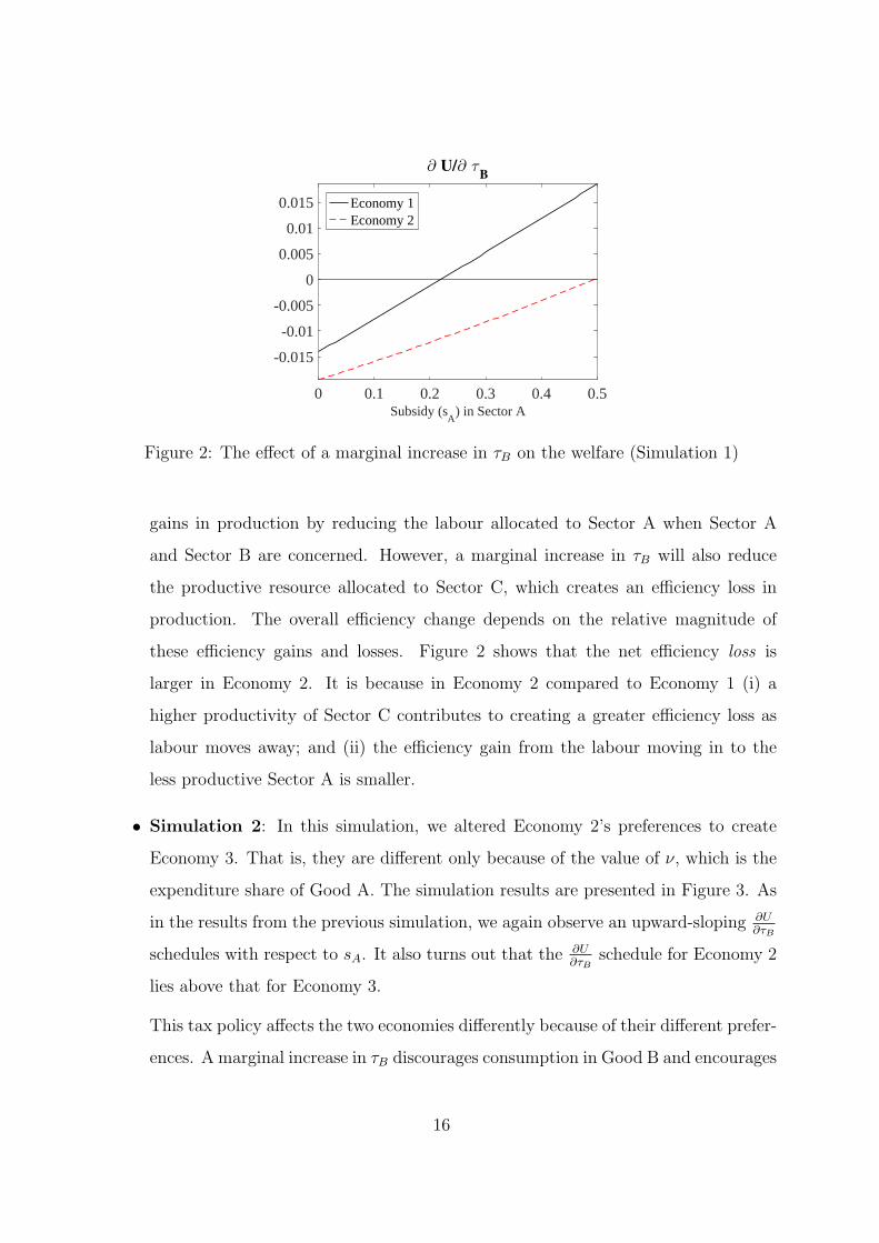
Figure 2 plots the ∂U∂τB

schedules for both economies, where the level of subsidy in

Sector A is measured on the horizontal axis. From the figure, we can gather two

bits of information. One is that the schedules are upward-sloping, meaning that

the welfare effect of a marginal increase in τB is more likely to be positive as sA

increases. Intuitively, the more protected Sector A is, the more likely adding an

extra distortion to Sector B alleviates the overall production inefficiency, and hence

improves economic welfare.

The other observation is that the ∂U∂τB

schedule for Economy 1 lies above that for

Economy 2. With the help of our intuition from the analytical section, we can

interpret this result as follows. Since sA ≥ 0 as well as τA > τB, Sector A is more

protected than Sector B. Hence, a marginal increase in τB will result in efficiency

15

0 0.1 0.2 0.3 0.4 0.5Subsidy (s

A) in Sector A

-0.015

-0.01

-0.005

0

0.005

0.01

0.015

∂ U/∂ τB

Economy 1Economy 2

Figure 2: The effect of a marginal increase in τB on the welfare (Simulation 1)

gains in production by reducing the labour allocated to Sector A when Sector A

and Sector B are concerned. However, a marginal increase in τB will also reduce

the productive resource allocated to Sector C, which creates an efficiency loss in

production. The overall efficiency change depends on the relative magnitude of

these efficiency gains and losses. Figure 2 shows that the net efficiency loss is

larger in Economy 2. It is because in Economy 2 compared to Economy 1 (i) a

higher productivity of Sector C contributes to creating a greater efficiency loss as

labour moves away; and (ii) the efficiency gain from the labour moving in to the

less productive Sector A is smaller.

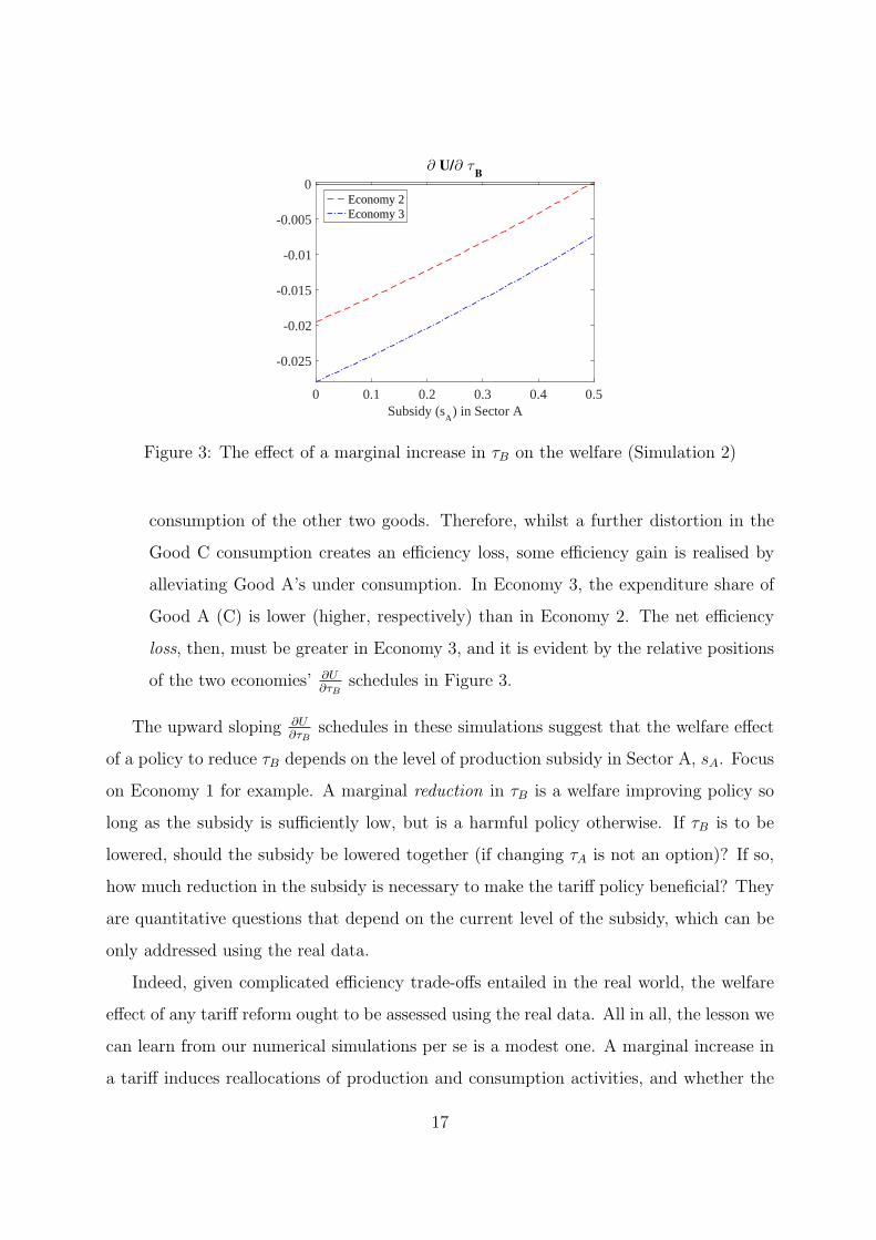
• Simulation 2: In this simulation, we altered Economy 2’s preferences to create

Economy 3. That is, they are different only because of the value of ν, which is the

expenditure share of Good A. The simulation results are presented in Figure 3. As

in the results from the previous simulation, we again observe an upward-sloping ∂U∂τB

schedules with respect to sA. It also turns out that the ∂U∂τB

schedule for Economy 2

lies above that for Economy 3.

This tax policy affects the two economies differently because of their different prefer-

ences. A marginal increase in τB discourages consumption in Good B and encourages

16

0 0.1 0.2 0.3 0.4 0.5Subsidy (s

A) in Sector A

-0.025

-0.02

-0.015

-0.01

-0.005

0∂ U/∂ τ

B

Economy 2Economy 3

Figure 3: The effect of a marginal increase in τB on the welfare (Simulation 2)

consumption of the other two goods. Therefore, whilst a further distortion in the

Good C consumption creates an efficiency loss, some efficiency gain is realised by

alleviating Good A’s under consumption. In Economy 3, the expenditure share of

Good A (C) is lower (higher, respectively) than in Economy 2. The net efficiency

loss, then, must be greater in Economy 3, and it is evident by the relative positions

of the two economies’ ∂U∂τB

schedules in Figure 3.

The upward sloping ∂U∂τB

schedules in these simulations suggest that the welfare effect

of a policy to reduce τB depends on the level of production subsidy in Sector A, sA. Focus

on Economy 1 for example. A marginal reduction in τB is a welfare improving policy so

long as the subsidy is sufficiently low, but is a harmful policy otherwise. If τB is to be

lowered, should the subsidy be lowered together (if changing τA is not an option)? If so,

how much reduction in the subsidy is necessary to make the tariff policy beneficial? They

are quantitative questions that depend on the current level of the subsidy, which can be

only addressed using the real data.

Indeed, given complicated efficiency trade-offs entailed in the real world, the welfare

effect of any tariff reform ought to be assessed using the real data. All in all, the lesson we

can learn from our numerical simulations per se is a modest one. A marginal increase in

a tariff induces reallocations of production and consumption activities, and whether the

17

policy is beneficial for the economy depends on whether a net efficiency gain is realised

after these reallocations. In the next section, we calibrate our model to the Japanese

economy to assess the welfare effect of a policy to reduce τB.

4 Calibrating our model to the Japanese economy

4.1 Adding a non-traded goods sector

So far our model only concerns traded-goods sectors. In calibrating our model to the

Japanese economy, this feature of our model may be problematic given the magnitude of

its service industry where a variety of non-traded goods are mainly produced. According

to the Updated Input-Output Table 2013 (Ministry of Economy, Trade and Industry,

Japan, 2013, IO Table hereafter), the service industry accounts for around 85 per cent of

the Japanese economy both in terms of the final demand and the number of employees. In

this paper we regard the service industry as the non-traded goods sector and incorporate

it into our three-sector model. Our four-sector specific factor model hence resembles the

specific factor model in Corden and Neary (1982), which has a non-traded goods sector

and two traded-goods sectors, except that ours has an extra import-competing sector (as

well as domestic distortion).

We denote the non-traded goods sector as N, and its production function is given as:

YN = LδNK

1−δN , (27)

where, LN is the labour allocated to Sector N, KN is the specific factor, and 0 < δ < 1.

Solving the producer’s profit maximisation problem, we obtain the following first-order

conditions.

w = PNδLδ−1N K1−δ

N , (28)

rN = PN(1− δ)LδNK

−δN . (29)

18

The labour market clearing condition is rewritten as:

LA + LB + LC + LN = L. (30)

Denoting the consumption of Good N as QN , the utility function is modified as:

U (QA, QB, QC , QN) = QνAQ

ϕBQ

ωCQ

1−ν−ϕ−ωN , (31)

where 0 < ν < 1, 0 < ϕ < 1, 0 < ω < 1, and 0 < ν + ϕ + ω < 1. The consumer’s utility

maximisation requires:

QA

QB

=ν

ϕ

PB(1 + τB)

PA(1 + τA), (32)

QB

QC

=ϕ

ω

PC

PB(1 + τB), (33)

QC

QN

=ω

1− ν − ϕ− ω

PN

PC

. (34)

The market-clearing condition for the non-traded goods sector is given as:

YN = QN . (35)

We also introduce a production subsidy sB in Sector B into our extended model as we

are interested in a counterfactual policy to marginally change sB. It is a useful counter-

factual experiment as we can isolate the welfare effect of a tariff change in Sector B that

is caused by a change in the producer relative prices.

In any event, the producer’s profit maximisation conditions involving Sector B has

now become the following.

w = PB(1 + τB) + sBβLβ−1B K1−β

B , (36)

rB = PB(1 + τB) + sB(1− β)LβBK

−βB . (37)

We set sB equal to zero in our calibration as the data suggest that the Sector B

19

subsidy is insignificant, and hence these equations are essentially identical to (17) and (18),

respectively. However, for the sake of accurately presenting our calibration exercise later

on, we use (36) and (37) as part of the equations that characterise the equilibrium of this

economy. Together with these two equations, (1), (2), (4)-(7), (13), (14), (16), (23), (24)

and (27)-(35) describe the equilibrium of this economy. Our calibration’s primary focus

is the partial derivative of U (QA, QB, QC , QN) in (31) with respect to τB:

∂U

∂τB= Qν

AQϕBQ

ωCQ

1−ν−ϕ−ωN

ν

1

QA

∂QA

∂τB+ ϕ

1

QB

∂QB

∂τB+ ω

1

QC

∂QC

∂τB+ (1− ν − ϕ− ω)

1

QN

∂QN

∂τB

.(38)

4.2 Calibration strategy

Our calibration strategy follows two main procedures. First, we determine the values of

the parameters which do not rely on the solution of the model, namely tariff rates (τA

and τB), the aggregate quantity of labour in the economy (L), the share of labour in each

sector (α, β, γ, and δ), and the levels of capital in each sector (KA, KB, KC , and KN).

Next, we calibrate remaining parameters, i.e. prices of the goods (PA, PB, PC , and PN),

the production subsidy in Sector A (sA), and the preference parameters (ν, ϕ, and ω), by

matching the equilibrium conditions of the model.

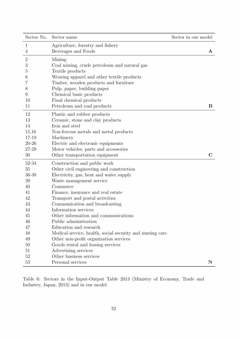
We use the Japanese data for 2013. Table 6 in Appendix A shows how we have

converted the 54 sectors in the IO Table in to our four sectors.6 As shown in Table 4 in

Appendix A, τA and τB are calculated as the weighted averages of average tariff rates of

product groups provided in World Tariff Profiles 2013 (WTO, ITC and UNCTAD, 2013).

To determine α, β, γ, and δ, we are guided by the following definition of labour share

in Sugou and Nishizaki (2002):

Labour share =Personnel expenses

Personnel expenses + Operating profit + Depreciation.

For personnel expenses, operating profit, and depreciation, we use the corresponding IO

6We have omitted Sector 30 (Other manufacturing) and Sector 54 (Activities not elsewhere classified).They account for less than one per cent of economic activities in Japan.

20

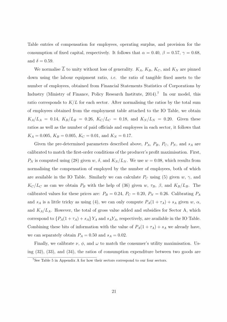
Table entries of compensation for employees, operating surplus, and provision for the

consumption of fixed capital, respectively. It follows that α = 0.40, β = 0.57, γ = 0.68,

and δ = 0.59.

We normalise L to unity without loss of generality. KA, KB, KC , and KN are pinned

down using the labour equipment ratio, i.e. the ratio of tangible fixed assets to the

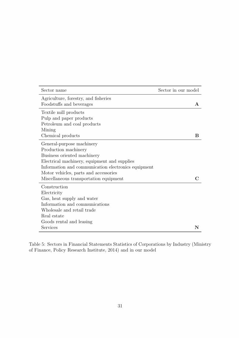
number of employees, obtained from Financial Statements Statistics of Corporations by

Industry (Ministry of Finance, Policy Research Institute, 2014).7 In our model, this

ratio corresponds to K/L for each sector. After normalising the ratios by the total sum

of employees obtained from the employment table attached to the IO Table, we obtain

KA/LA = 0.14, KB/LB = 0.26, KC/LC = 0.18, and KN/LN = 0.20. Given these

ratios as well as the number of paid officials and employees in each sector, it follows that

KA = 0.005, KB = 0.005, KC = 0.01, and KN = 0.17.

Given the pre-determined parameters described above, PA, PB, PC , PN , and sA are

calibrated to match the first-order conditions of the producer’s profit maximisation. First,

PN is computed using (28) given w, δ, and KN/LN . We use w = 0.08, which results from

normalising the compensation of employed by the number of employees, both of which

are available in the IO Table. Similarly we can calculate PC using (5) given w, γ, and

KC/LC as can we obtain PB with the help of (36) given w, τB, β, and KB/LB. The

calibrated values for these prices are: PB = 0.24, PC = 0.20, PN = 0.26. Calibrating PA

and sA is a little tricky as using (4), we can only compute PA(1 + τA) + sA given w, α,

and KA/LA. However, the total of gross value added and subsidies for Sector A, which

correspond to PA(1 + τA) + sAYA and sAYA, respectively, are available in the IO Table.

Combining these bits of information with the value of PA(1 + τA) + sA we already have,

we can separately obtain PA = 0.50 and sA = 0.02.

Finally, we calibrate ν, ϕ, and ω to match the consumer’s utility maximisation. Us-

ing (32), (33), and (34), the ratios of consumption expenditure between two goods are

7See Table 5 in Appendix A for how their sectors correspond to our four sectors.

21

described as:

PA(1 + τA)QA

PB(1 + τB)QB

=ν

ϕ, (39)

PB(1 + τB)QB

PCQC

=ϕ

ω, (40)

PCQC

PNQN

=ω

1− ν − ϕ− ω. (41)

We obtain the values of private consumption expenditure of each sector from the IO Table

and substitute them into the left hand side of each of these equations. Then (39), (40),

and (41) together become a system of three equations with three unknowns, namely ν, ϕ,

and ω. Solving this system, we obtain ν = 0.10, ϕ = 0.04, and ω = 0.05.

4.3 Results

Figure 4 illustrates the ∂U∂τB

schedule for the Japanese economy.

0 0.01 0.02 0.03 0.04 0.05Subsidy in Sector A (s

A)

0

2

4

6

8×10-4 ∂ U/∂ τ

B

∂ U/∂ τB

Figure 4: The welfare effect of an increase in τB on the Japanese economy

It shows, given the calibrated value of the production subsidy in Sector A, sA = 0.02,

that a marginal reduction in τB is harmful for the Japanese economy. In fact, even if the

production subsidy in Sector A is completely removed, a marginal reduction in τB is still

harmful for the Japanese economy. It indicates that τA is so high that Sector A is much

22

more protected than Sector B is, even after sA is fully removed.

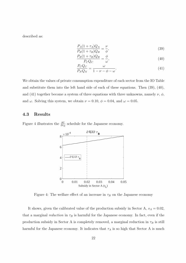
To get a better sense of Sector A’s high protection, we ask the following question.

How much reduction in τA is necessary to render the marginal reduction in τB welfare

improving? It turns out that, to have ∂U∂τB

= 0 when sA = 0.02, τA needs to be more

than halved (τA = 0.10). Given τA = 0.10, the counterfactual ∂U∂τB

schedule is illustrated

in Figure 5. It indicates that, if τA = 0.10, then the policy to marginally reduce τB

accompanied by a reduction in sA would be beneficial for the Japanese economy.


A)

-1

0

1

2

×10-4 ∂ U/∂ τB

(∂ U/∂ τB

when τA

=0.10)

Figure 5: Counterfactual welfare effect of an increase in τB on the Japanese economywhen τA = 0.10

A marginal reduction in τB lowers Sector B’s protection, but lowering sB can do the

same job. However, these two policies are different in that whilst the former affects the

relative prices that both consumers and producers face, the latter only affects the relative

prices faced by producers. Hence we can decompose the welfare effect of a marginal

reduction in τB into two components: (i) the effect which is caused by sB; and (ii) the

remaining effect. Since the first effect is brought about by the resource reallocation in

production only, the remaining effect can be interpreted as that caused by the change in

consumption choice.

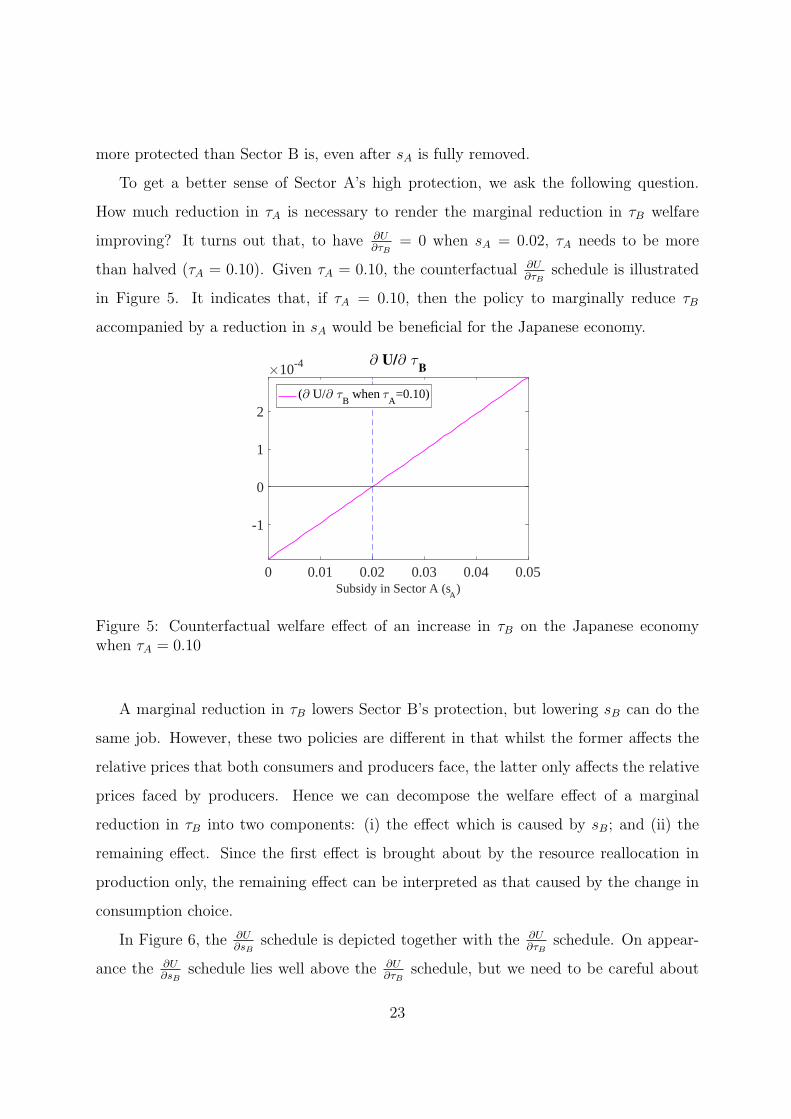
In Figure 6, the ∂U∂sB

schedule is depicted together with the ∂U∂τB

schedule. On appear-

ance the ∂U∂sB

schedule lies well above the ∂U∂τB

schedule, but we need to be careful about

23


A)

0

1

2

3

4

5

6×10-3 ∂ U/∂ τ

B and ∂ U/∂ s

B

∂ U/∂ τB

∂ U/∂ sB

Figure 6: The welfare effect of an increase in sB on the Japanese economy

comparing these welfare effects. Note that whilst a marginal increase in sB affects the

producer price of Good B by dsB, a marginal increase in τB increases the producer price

of Good by PBdτB. Therefore, if we want to examine the comparable welfare effect of dτB

only on the production side, we need to focus on the welfare effect of dsB multiplied by

PB.


A)

0

0.1

0.2

0.3

0.4

0.5

0.6

(∂ U/∂ sB

)PB

/(∂ U/∂ τB

)

(∂ U/∂ sB

)PB

/(∂ U/∂ τB

)

Figure 7: Comparison of two policies to protect Sector B

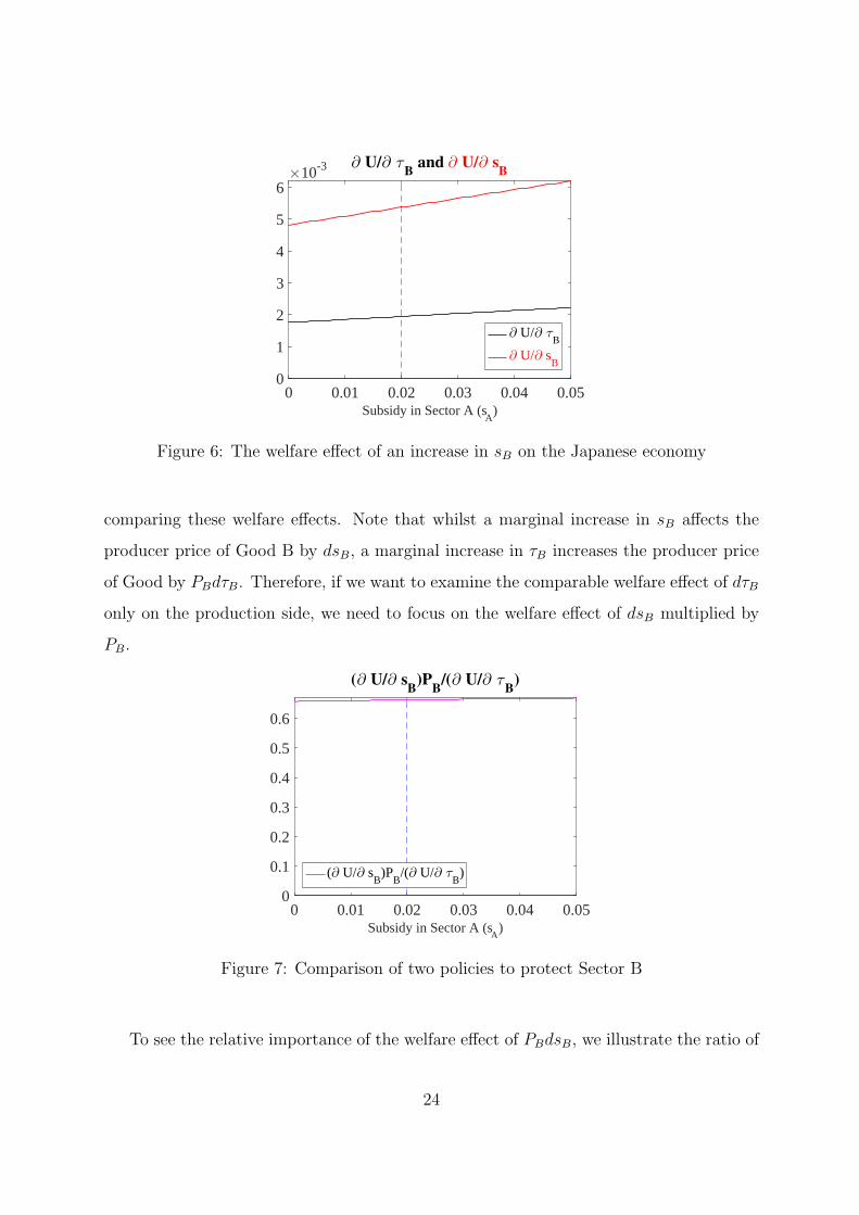
To see the relative importance of the welfare effect of PBdsB, we illustrate the ratio of

24

∂U∂sB

PB and ∂U∂τB

in Figure 7. This figure and Figure 4 indicate that: (i) a marginal reduction

in τB, for the calibrated value of the production subsidy in Sector A (sA = 0.02), harms the

Japanese economy by creating further distortions both on production and consumption

sides; and (ii) roughly 70 per cent of the (negative) welfare effect is attributable to further

inefficient resource allocations on the production side.

5 Conclusion

Agricultural producer support in Japan is distinctive in terms of both tariffs imposed

on agricultural products and the government subsidy, whilst both forms of protection in

other import-competing sectors are rather modest. To incorporate these characteristics of

the Japanese economy, we have constructed a specific factor model that has two import-

competing sectors, both of which are protected by tariffs but only one of them enjoys a

production subsidy. Perhaps, often politically, since the protection in the most heavily

protected sector is hugely costly to be reduced, a general movement towards freetrade

tends to end up in a tariff reduction only in modestly protected sectors, which we view

as the outcome of the recent TPP negotiations. Using our model, we have examined the

welfare effect of a policy to reduce a tariff in the less protected sector, by calibrating it to

the 2013 Japanese economy.

Our calibration result suggests that the partial tariff reduction policy is harmful by

making both production and consumption activities inefficient where the former explains

roughly 70 per cent of the overall inefficiency losses. A complete removal of the production

subsidy in the agricultural sector hardly changes the negative welfare effect of this tariff

policy, which is indicative of the enormity of the tariff protection in the agricultural sector.

Indeed, for the partial tariff reduction policy to be welfare improving, ceteris paribus, the

tariff in the agricultural sector must be more than halved.

Our specific factor model is tractable, which helps follow and interpret our calibration

results clearly. However, the use of a simple economic model imposes some limitations. For

example, a specific factor model assumes a set of fixed international prices, i.e. a country

25

in question is considered a small open economy, but whether it is applied to Japan is

debatable. A similar analysis may be conducted by constructing a two-country model,

where the prices of the traded-goods are also endogenously determined, but whatever

result that comes out of it could be difficult to interpret. A set of fixed international

prices also implies that no tariff change has occurred elsewhere. Of course, in reality, trade

policy negotiations occur with other economies, and our setup is restricted to examining

a unilateral tariff reform. These agenda are beyond the scope of the current paper and

are left for future research.

26

References

Abe, K., “Tariff Reform in a Small Open Economy with Public Production,” Interna-

tional Economic Review 33 (1992), 209–22.

Anderson, J. E. and J. P. Neary, “Welfare versus market access: The implications

of tariff structure for tariff reform,” Journal of International Economics 71 (2007), 187

– 205.

Bhagwati, J., “Non-economic Objectives and the Efficiency Properties of Trade,” Jour-

nal of Political Economy 75 (1967), 738–42.

Bhagwati, J. and V. K. Ramaswami, “Domestic Distortions, Tariffs and the Theory

of Optimum Subsidy,” Journal of Political Economy 71 (1963), 44–50.

Bruno, M., “Market Distortions and Gradual Reform,” The Review of Economic Studies

39 (1972), 373–83.

Corden, W., “The normative theory of international trade,” in R. W. Jones and P. B.

Kenen, eds., Handbook of International Economics, vol. 1 (Elsevier, 1984), 63–130.

Corden, W. M. and J. P. Neary, “Booming Sector and De-Industrialisation in a

Small Open Economy,” The Economic Journal 92 (1982), 825–48.

Diewert, W. E., A. H. Turunen-Red and A. D. Woodland, “Tariff Reform in

a Small Open Multi-Household Economy with Domestic Distortions and Nontraded

Goods,” International Economic Review 32 (1991), 937–57.

Dixit, A., “Tax policy in open economies,” in A. J. Auerbach and M. Feldstein, eds.,

Handbook of Public Economics, vol. 1 (Elsevier, 1985).

Falvey, R. and U. Kreickemeier, “The Theory of Trade Policy,” in D. Greenaway,

R. Falvey, U. Kreickemeier and D. Bernhofen, eds., Palgrave Handbook of International

Trade (Palgrave Macmillan UK, 2013), 265–94.

27

Foster, E. and H. Sonnenschein, “Price Distortion and Economic Welfare,” Econo-

metrica 38 (1970), 281–97.

Fukushima, T., “Tariff Structure, Nontraded Goods and Theory of Piecemeal Policy

Recommendations,” International Economic Review 20 (1979), 427–35.

Hagen, E. E., “An Economic Justification of Protectionism,” The Quarterly Journal of

Economics 72 (1958), 496–514.

Hatta, T., “A Recommendation for a Better Tariff Structure,” Econometrica 45 (1977a),

1859–69.

———, “A Theory of Piecemeal Policy Recommendations,” The Review of Economic

Studies 44 (1977b), 1–21.

Johnson, H. G., “Factor Market Distortions and the Shape of the Transformation

Curve,” Econometrica 34 (1966), 686–98.

Jones, R. W., “Distortions in Factor Markets and the General Equilibrium Model of

Production,” Journal of Political Economy 79 (1971a), 437–59.

———, “A Three-factor Model in Theory, Trade, and History,” in J. Bhagwati, R. Jones,

R. Mundell and J. Vanek, eds., Trade, balance of payments and growth: papers in

international economics in honor of Charles P. Kindleberger (North-Holland, 1971b),

3–21.

Ju, J. and K. Krishna, “Welfare and market access effects of piecemeal tariff reform,”

Journal of International Economics 51 (2000), 305–316.

Lipsey, R. G. and K. Lancaster, “The General Theory of Second Best,” The Review

of Economic Studies 24 (1956), 11–32.

Ministry of Economy, Trade and Industry, Japan, “Updated Input-

Output Tables 2013,” http://www.meti.go.jp/statistics/tyo/entyoio/result.

html#entyo_h17 (2013), (Accessed on 24 April 2017).

28

Ministry of Finance, Policy Research Institute, “Financial Statements

Statistics of Corporations by Industry,” http://www.mof.go.jp/pri/publication/

zaikin_geppo/hyou/g762/762.htm (2014), (Accessed on 24 April 2017).

Mussa, M., “Tariffs and the Distribution of Income: The Importance of Factor Speci-

ficity, Substitutability, and Intensity in the Short and Long Run,” Journal of Political

Economy 82 (1974), 1191–203.

OECD, “Agricultural support (indicator),” doi:10.1787/6ea85c58-en (2017), (Ac-

cessed on 13 April 2017).

Ohyama, M., “Domestic Distortions and the Theory of Tariffs,” Keio Economic Studies

9 (1972), 1–14.

Sugou, T. and K. Nishizaki, “Waga kuni ni okeru roudou bumpairitsu ni tsuite no

ichikousatsu (An Analysis on the Share of Labour in Japan),” Kin’yu Kenkyu 21 (2002),

125–69.

Turunen-Red, A. H. and A. D. Woodland, “Strict Pareto-Improving Multilateral

Reforms of Tariffs,” Econometrica 59 (1991), 1127–52.

Vousden, N., The Economics of Trade Protection (Cambridge University Press, 1990).

WTO, ITC and UNCTAD, “World Tariff Profiles 2013,” https://www.wto.org/

english/res_e/publications_e/world_tariff_profiles13_e.htm (2013), (Ac-

cessed on 13 April 2017).

29

Appendix A Sector classification

Product group Ave. tariff (%) Import share (%) Sector in our model

Animal products 13.6 1.6Dairy products 116.9 0.2Fruit, vegetables, plants 9.9 1.1Coffee, tea 14.4 0.4Cereals & preparations 80.2 1.6Oilseeds, fats & oils 9.8 0.8Sugars and confectionery 50.2 0.2Beverages & tobacco 16.8 1.2Cotton 0 0Other agricultural products 5.4 0.7Fish & fish products 4.9 2.1

(τA = 24.4) A

Minerals & Metals 1 24.5Petroleum 8.2 20.2Wood, paper, etc. 1 2.9Textiles 5.6 1.9Clothing 9.2 3.7Chemicals 2.3 9.3

(τB = 4.1) B

Non-electrical machinery 0 7.7Electrical machinery 0.2 10.3Transport equipment 0 2.6 C

Table 4: Product groups in World Tariff Profiles 2013 (WTO, ITC and UNCTAD, 2013)and traded-goods sectors in our model

30

Sector name Sector in our model

Agriculture, forestry, and fisheriesFoodstuffs and beverages A

Textile mill productsPulp and paper productsPetroleum and coal productsMiningChemical products B

General-purpose machineryProduction machineryBusiness oriented machineryElectrical machinery, equipment and suppliesInformation and communication electronics equipmentMotor vehicles, parts and accessoriesMiscellaneous transportation equipment C

ConstructionElectricityGas, heat supply and waterInformation and communicationsWholesale and retail tradeReal estateGoods rental and leasingServices N

Table 5: Sectors in Financial Statements Statistics of Corporations by Industry (Ministryof Finance, Policy Research Institute, 2014) and in our model

31

Sector No. Sector name Sector in our model

1 Agriculture, forestry and fishery4 Beverages and Foods A

2 Mining3 Coal mining, crude petroleum and natural gas5 Textile products6 Wearing apparel and other textile products7 Timber, wooden products and furniture8 Pulp, paper, building paper9 Chemical basic products10 Final chemical products11 Petroleum and coal products B

12 Plastic and rubber products13 Ceramic, stone and clay products14 Iron and steel15,16 Non-ferrous metals and metal products17-19 Machinery20-26 Electric and electronic equipments27-29 Motor vehicles, parts and accessories30 Other transportation equipment C

32-34 Construction and public work35 Other civil engineering and construction36-38 Electricity, gas, heat and water supply39 Waste management service40 Commerce41 Finance, insurance and real estate42 Transport and postal activities43 Communication and broadcasting44 Information services45 Other information and communications46 Public administration47 Education and research48 Medical service, health, social security and nursing care49 Other non-profit organization services50 Goods rental and leasing services51 Advertising services52 Other business services53 Personal services N

Table 6: Sectors in the Input-Output Table 2013 (Ministry of Economy, Trade andIndustry, Japan, 2013) and in our model

32

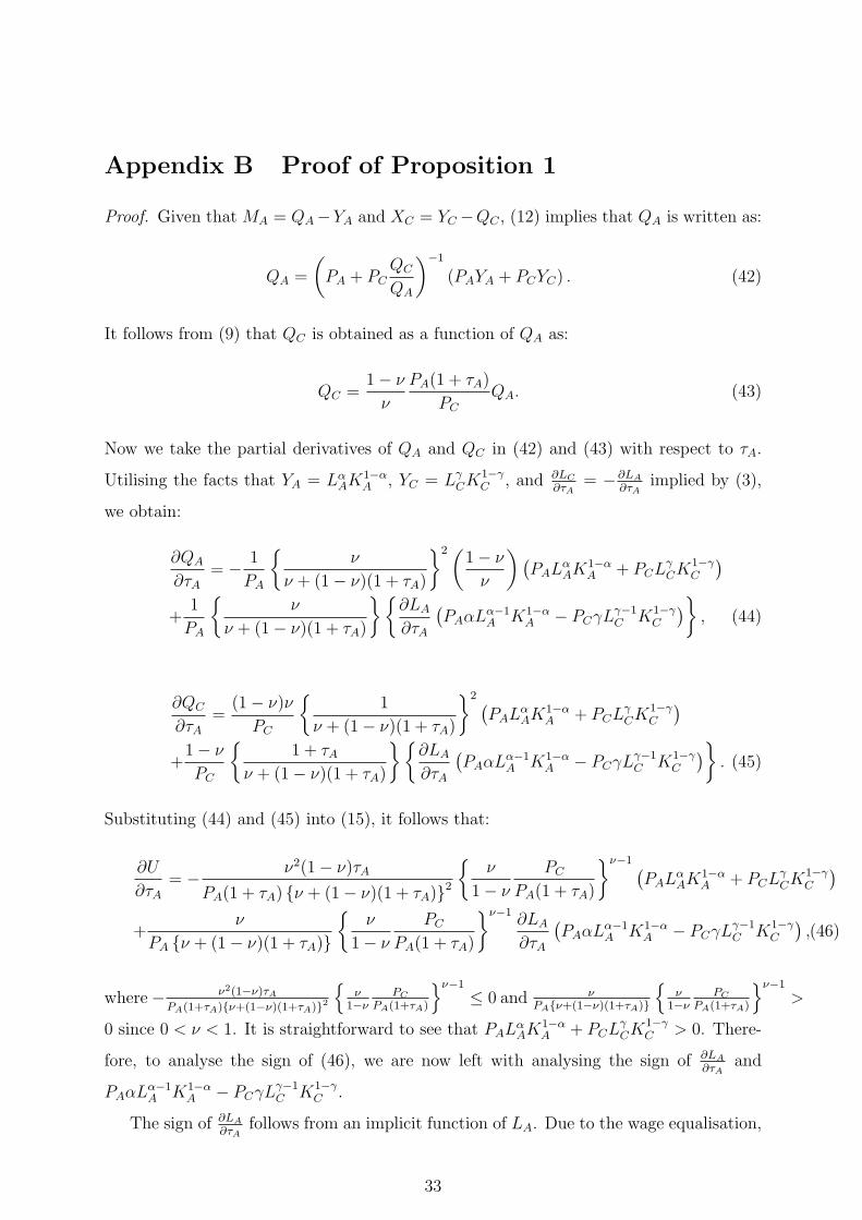
Appendix B Proof of Proposition 1

Proof. Given that MA = QA−YA and XC = YC −QC , (12) implies that QA is written as:

QA =

(PA + PC

QC

QA

)−1

(PAYA + PCYC) . (42)

It follows from (9) that QC is obtained as a function of QA as:

QC =1− ν

ν

PA(1 + τA)

PC

QA. (43)

Now we take the partial derivatives of QA and QC in (42) and (43) with respect to τA.

Utilising the facts that YA = LαAK

1−αA , YC = Lγ

CK1−γC , and ∂LC

∂τA= −∂LA

∂τAimplied by (3),

we obtain:

∂QA

∂τA= − 1

PA

ν

ν + (1− ν)(1 + τA)

2(1− ν

ν

)(PAL

αAK

1−αA + PCL

γCK

1−γC

)+

1

PA

ν

ν + (1− ν)(1 + τA)

∂LA

∂τA

(PAαL

α−1A K1−α

A − PCγLγ−1C K1−γ

C

), (44)

∂QC

∂τA=

(1− ν)ν

PC

1

ν + (1− ν)(1 + τA)

2 (PAL

αAK

1−αA + PCL

γCK

1−γC

)+1− ν

PC

1 + τA

ν + (1− ν)(1 + τA)

∂LA

∂τA

(PAαL

α−1A K1−α


C

). (45)

Substituting (44) and (45) into (15), it follows that:

∂U

∂τA= − ν2(1− ν)τA

PA(1 + τA) ν + (1− ν)(1 + τA)2

ν

1− ν

PC

PA(1 + τA)

ν−1 (PAL

αAK

1−αA + PCL

γCK

1−γC

)+

ν

PA ν + (1− ν)(1 + τA)

ν

1− ν

PC

PA(1 + τA)

ν−1∂LA

∂τA

(PAαL

α−1A K1−α


C

),(46)

where− ν2(1−ν)τAPA(1+τA)ν+(1−ν)(1+τA)2

ν

1−νPC

PA(1+τA)

ν−1

≤ 0 and νPAν+(1−ν)(1+τA)

ν

1−νPC

PA(1+τA)

ν−1

>

0 since 0 < ν < 1. It is straightforward to see that PALαAK

1−αA + PCL

γCK

1−γC > 0. There-

fore, to analyse the sign of (46), we are now left with analysing the sign of ∂LA

∂τAand

PAαLα−1A K1−α


C .

The sign of ∂LA

∂τAfollows from an implicit function of LA. Due to the wage equalisation,

33

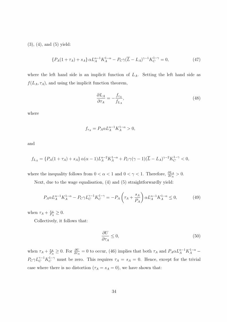
(3), (4), and (5) yield:

PA(1 + τA) + sAαLα−1A K1−α

A − PCγ(L− LA)γ−1K1−γ

C = 0, (47)

where the left hand side is an implicit function of LA. Setting the left hand side as

f(LA, τA), and using the implicit function theorem,

∂LA

∂τA= − fτA

fLA

, (48)

where

fτA = PAαLα−1A K1−α

A > 0,

and

fLA= PA(1 + τA) + sAα(α− 1)Lα−2

A K1−αA + PCγ(γ − 1)(L− LA)

γ−2K1−γC < 0,

where the inequality follows from 0 < α < 1 and 0 < γ < 1. Therefore, ∂LA

∂τA> 0.

Next, due to the wage equalisation, (4) and (5) straightforwardly yield:

PAαLα−1A K1−α


C = −PA

(τA +

sAPA

)αLα−1

A K1−αA ≤ 0, (49)

when τA + sAPA

≥ 0.

Collectively, it follows that:

∂U

∂τA≤ 0, (50)

when τA + sAPA

≥ 0. For ∂U∂τA

= 0 to occur, (46) implies that both τA and PAαLα−1A K1−α

A −

PCγLγ−1C K1−γ

C must be zero. This requires τA = sA = 0. Hence, except for the trivial

case where there is no distortion (τA = sA = 0), we have shown that:

34

∂U

∂τA< 0,

for any sA ≥ 0.

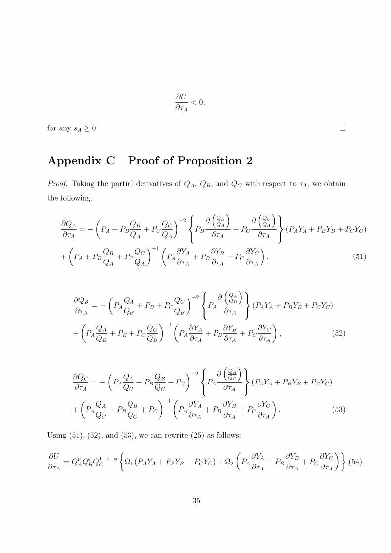
Appendix C Proof of Proposition 2

Proof. Taking the partial derivatives of QA, QB, and QC with respect to τA, we obtain

the following.

∂QA

∂τA= −

(PA + PB

QB

QA

+ PCQC

QA

)−2

PB

∂(

QB

QA

)∂τA

+ PC

∂(

QC

QA

)∂τA

(PAYA + PBYB + PCYC)

+

(PA + PB

QB

QA

+ PCQC

QA

)−1(PA

∂YA

∂τA+ PB

∂YB

∂τA+ PC

∂YC

∂τA

), (51)

∂QB

∂τA= −

(PA

QA

QB

+ PB + PCQC

QB

)−2

PA

∂(

QA

QB

)∂τA


+

(PA

QA

QB

+ PB + PCQC

QB

)−1(PA

∂YA

∂τA+ PB

∂YB

∂τA+ PC

∂YC

∂τA

), (52)

∂QC

∂τA= −

(PA

QA

QC

+ PBQB

QC

+ PC

)−2

PA

∂(

QA

QC

)∂τA


+

(PA

QA

QC

+ PBQB

QC

+ PC

)−1(PA

∂YA

∂τA+ PB

∂YB

∂τA+ PC

∂YC

∂τA

). (53)

Using (51), (52), and (53), we can rewrite (25) as follows:

∂U

∂τA= Qν

AQϕBQ

1−ν−ϕC

Ω1 (PAYA + PBYB + PCYC) + Ω2

(PA

∂YA

∂τA+ PB

∂YB

∂τA+ PC

∂YC

∂τA

),(54)

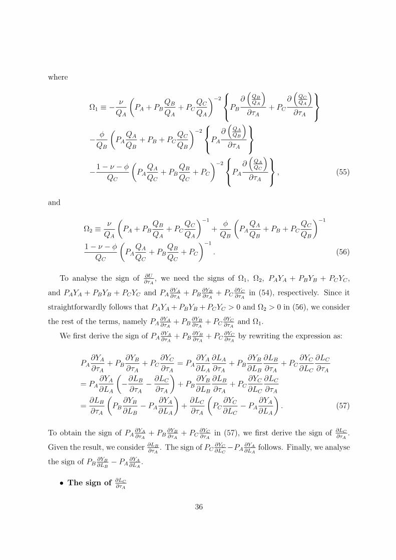
35

where

Ω1 ≡ − ν

QA

(PA + PB

QB

QA

+ PCQC

QA

)−2

PB

∂(

QB

QA

)∂τA

+ PC

∂(

QC

QA

)∂τA

− ϕ

QB

(PA

QA

QB

+ PB + PCQC

QB

)−2

PA

∂(

QA

QB

)∂τA

−1− ν − ϕ

QC

(PA

QA

QC

+ PBQB

QC

+ PC

)−2

PA

∂(

QA

QC

)∂τA

, (55)

and

Ω2 ≡ν

QA

(PA + PB

QB

QA

+ PCQC

QA

)−1

+ϕ

QB

(PA

QA

QB

+ PB + PCQC

QB

)−1

1− ν − ϕ

QC

(PA

QA

QC

+ PBQB

QC

+ PC

)−1

. (56)

To analyse the sign of ∂U∂τA

, we need the signs of Ω1, Ω2, PAYA + PBYB + PCYC ,

and PAYA + PBYB + PCYC and PA∂YA

∂τA+ PB

∂YB

∂τA+ PC

∂YC

∂τAin (54), respectively. Since it

straightforwardly follows that PAYA +PBYB +PCYC > 0 and Ω2 > 0 in (56), we consider

the rest of the terms, namely PA∂YA

∂τA+ PB

∂YB

∂τA+ PC

∂YC

∂τAand Ω1.

We first derive the sign of PA∂YA

∂τA+ PB

∂YB

∂τA+ PC

∂YC

∂τAby rewriting the expression as:

PA∂YA

∂τA+ PB

∂YB

∂τA+ PC

∂YC

∂τA= PA

∂YA

∂LA

∂LA

∂τA+ PB

∂YB

∂LB

∂LB

∂τA+ PC

∂YC

∂LC

∂LC

∂τA

= PA∂YA

∂LA

(−∂LB

∂τA− ∂LC

∂τA

)+ PB

∂YB

∂LB

∂LB

∂τA+ PC

∂YC

∂LC

∂LC

∂τA

=∂LB

∂τA

(PB

∂YB

∂LB

− PA∂YA

∂LA

)+

∂LC

∂τA

(PC

∂YC

∂LC

− PA∂YA

∂LA

). (57)

To obtain the sign of PA∂YA

∂τA+ PB

∂YB

∂τA+ PC

∂YC

∂τAin (57), we first derive the sign of ∂LC

∂τA.

Given the result, we consider ∂LB

∂τA. The sign of PC

∂YC

∂LC−PA

∂YA

∂LAfollows. Finally, we analyse

the sign of PB∂YB

∂LB− PA

∂YA

∂LA.

• The sign of ∂LC

∂τA

36

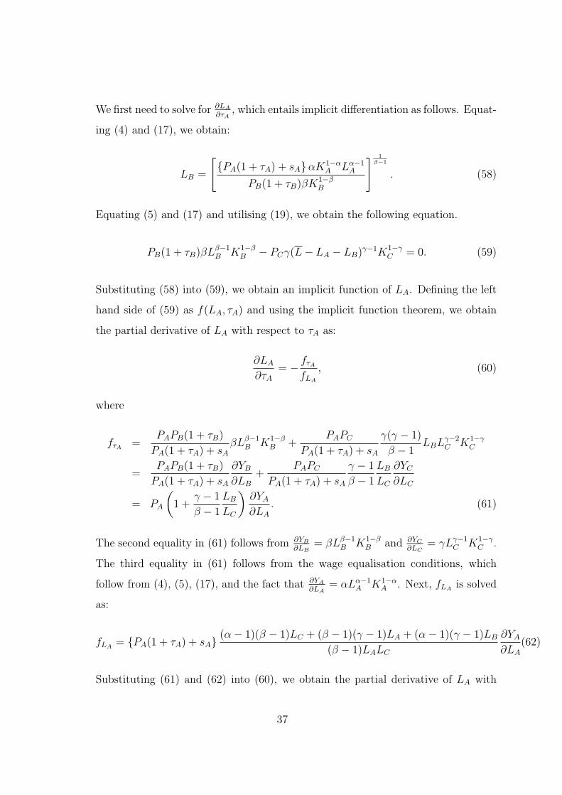
We first need to solve for ∂LA

∂τA, which entails implicit differentiation as follows. Equat-

ing (4) and (17), we obtain:

LB =

[PA(1 + τA) + sAαK1−α

A Lα−1A

PB(1 + τB)βK1−βB

] 1β−1

. (58)

Equating (5) and (17) and utilising (19), we obtain the following equation.

PB(1 + τB)βLβ−1B K1−β

B − PCγ(L− LA − LB)γ−1K1−γ

C = 0. (59)

Substituting (58) into (59), we obtain an implicit function of LA. Defining the left

hand side of (59) as f(LA, τA) and using the implicit function theorem, we obtain

the partial derivative of LA with respect to τA as:

∂LA

∂τA= − fτA

fLA

, (60)

where

fτA =PAPB(1 + τB)

PA(1 + τA) + sAβLβ−1

B K1−βB +

PAPC

PA(1 + τA) + sA

γ(γ − 1)

β − 1LBL

γ−2C K1−γ

C

=PAPB(1 + τB)

PA(1 + τA) + sA

∂YB

∂LB

+PAPC

PA(1 + τA) + sA

γ − 1

β − 1

LB

LC

∂YC

∂LC

= PA

(1 +

γ − 1

β − 1

LB

LC

)∂YA

∂LA

. (61)

The second equality in (61) follows from ∂YB

∂LB= βLβ−1

B K1−βB and ∂YC

∂LC= γLγ−1

C K1−γC .

The third equality in (61) follows from the wage equalisation conditions, which

follow from (4), (5), (17), and the fact that ∂YA

∂LA= αLα−1

A K1−αA . Next, fLA

is solved

as:

fLA= PA(1 + τA) + sA

(α− 1)(β − 1)LC + (β − 1)(γ − 1)LA + (α− 1)(γ − 1)LB

(β − 1)LALC

∂YA

∂LA

(62)

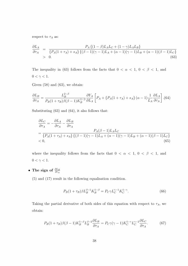
Substituting (61) and (62) into (60), we obtain the partial derivative of LA with

37

respect to τA as:

∂LA

∂τA=

PA (1− β)LALC + (1− γ)LALBPA(1 + τA) + sA (β − 1)(γ − 1)LA + (α− 1)(γ − 1)LB + (α− 1)(β − 1)LC

> 0. (63)

The inequality in (63) follows from the facts that 0 < α < 1, 0 < β < 1, and

0 < γ < 1.

Given (58) and (63), we obtain:

∂LB

∂τA=

L2−βB

PB(1 + τB)β(β − 1)K1−βB

∂YA

∂LA

[PA + PA(1 + τA) + sA (α− 1)

1

LA

∂LA

∂τA

].(64)

Substituting (63) and (64), it also follows that:

∂LC

∂τA= −∂LA

∂τA− ∂LB

∂τA

=PA(β − 1)LALC

PA(1 + τA) + sA (β − 1)(γ − 1)LA + (α− 1)(γ − 1)LB + (α− 1)(β − 1)LC< 0, (65)

where the inequality follows from the facts that 0 < α < 1, 0 < β < 1, and

0 < γ < 1.

• The sign of ∂LB

∂τA

(5) and (17) result in the following equalisation condition.

PB(1 + τB)βLβ−1B K1−β

B = PCγLγ−1C K1−γ

C . (66)

Taking the partial derivative of both sides of this equation with respect to τA, we

obtain:

PB(1 + τB)β(β − 1)K1−βB Lβ−2

B

∂LB

∂τA= PCγ(γ − 1)K1−γ

C Lγ−2C

∂LC

∂τA. (67)

38

Since ∂LC

∂τA< 0 as obtained in (65) and 0 < γ < 1, the right hand side of (67) is

positive. Since 0 < β < 1, from the left hand side of (67), we obtain:

∂LB

∂τA< 0. (68)

• The sign of PC∂YC

∂LC− PA

∂YA

∂LA

From the wage equalisation implied by (4) and (5) it follows that:

PC∂YC

∂LC

− PA∂YA

∂LA

= PCγLγ−1C K1−γ

C − PAαLα−1A K1−α

A

= PA

(τA +

sAPA

)αLα−1

A K1−αA ≥ 0, (69)

when τA + sAPA

≥ 0.

• The sign of PB∂YB

∂LB− PA

∂YA

∂LA

(4) and (17) yield

PB∂YB

∂LB

− PA∂YA

∂LA

= PBβLβ−1B K1−β

B − PAαLα−1A K1−α

A

=

PA(1 + τA) + sA − PA(1 + τB)

1 + τB

αLα−1

A K1−αA ≥ 0,

when τA + sAPA

≥ τB.

Therefore, (57), (65), (68), (69), and (70) together imply that:

PA∂YA

∂τA+ PB

∂YB

∂τA+ PC

∂YC

∂τA≤ 0 when τA +

sAPA

≥ τB. (70)

We are left with the analysis of the sign of Ω1 in (54). Following from (55) and using

39

(21), (22), and their partial derivatives with respect to τA, Ω1 is further written as

Ω1 = − 1

(PAQA + PBQB + PCQC)2[

QA

ϕPA

1 + τB+ (1− ν − ϕ)PA

−QB

νPB(1 + τB)

(1 + τA)2−QC

νPC

(1 + τA)2

]= − 1


PAQA

(1 + τA)(1 + τB)ϕ(τA − τB) + (1− ν − ϕ)τA(1 + τB)

]. (71)

Therefore, it follows that:

Ω1 ≤ 0 if ϕ(τA − τB) + (1− ν − ϕ)τA(1 + τB) ≥ 0. (72)

Finally, using (70) and (72), we obtain from (54) that:

∂U

∂τA≤ 0 if ϕ(τA − τB) + (1− ν − ϕ)τA(1 + τB) ≥ 0 and τA +

sAPA

≥ τB. (73)

Now, for ∂U∂τA

= 0 to occur, (54) suggests that both Ω1 and PA∂YA

∂τA+ PB

∂YB

∂τA+ PC

∂YC

∂τA

must be zero. It follows from (70) and (72) that it requires τA = τB = sA = 0. Hence,

except for the trivial case where there is no distortion (τA = τB = sA = 0), we have shown

that for any sA,

∂U

∂τA< 0 if ϕ(τA − τB) + (1− ν − ϕ)τA(1 + τB) ≥ 0 and τA +

sAPA

≥ τB. (74)

40

Appendix D Proof of Proposition 3

Proof. Taking the partial derivatives of QA, QB, and QC with respect to τB, we obtain

the following.

∂QA

∂τB= −

(PA + PB

QB

QA

+ PCQC

QA

)−2PB

∂(

QB

QA

)∂τB


+

(PA + PB

QB

QA

+ PCQC

QA

)−1(PA

∂YA

∂τB+ PB

∂YB

∂τB+ PC

∂YC

∂τB

), (75)

∂QB

∂τB= −

(PA

QA

QB

+ PB + PCQC

QB

)−2PA

∂(

QA

QB

)∂τB

+ PC

∂(

QC

QB

)∂τB


+

(PA

QA

QB

+ PB + PCQC

QB

)−1(PA

∂YA

∂τB+ PB

∂YB

∂τB+ PC

∂YC

∂τB

), (76)

∂QC

∂τB= −

(PA

QA

QC

+ PBQB

QC

+ PC

)−2PB

∂(

QB

QC

)∂τB


+

(PA

QA

QC

+ PBQB

QC

+ PC

)−1(PA

∂YA

∂τB+ PB

∂YB

∂τB+ PC

∂YC

∂τB

). (77)

Using (75), (76), and (77), we can rewrite (26) as follows.

∂U

∂τB= Qν

AQϕBQ

1−ν−ϕC

Ω3 (PAYA + PBYB + PCYC) + Ω2

(PA

∂YA

∂τB+ PB

∂YB

∂τB+ PC

∂YC

∂τB

),(78)

41

where

Ω3 ≡ − ν

QA

(PA + PB

QB

QA

+ PCQC

QA

)−2PB

∂(

QB

QA

)∂τB

− ϕ

QB

(PA

QA

QB

+ PB + PCQC

QB

)−2PA

∂(

QA

QB

)∂τB

+ PC

∂(

QC

QB

)∂τB

−1− ν − ϕ

QC

(PA

QA

QC

+ PBQB

QC

+ PC

)−2PB

∂(

QB

QC

)∂τB

. (79)

It is straightforward to see that PAYA + PBYB + PCYC > 0 and Ω2 > 0, which is defined

in (56). To analyse the sign of ∂U∂τB

, we further need the signs of Ω3 and PA∂YA

∂τB+PB

∂YB

∂τB+

PC∂YC

∂τBin (78).

We first derive the sign of PA∂YA

∂τB+ PB

∂YB

∂τB+ PC

∂YC

∂τBby rewriting the expression as:

PA∂YA

∂τB+ PB

∂YB

∂τB+ PC

∂YC

∂τB= PA

∂YA

∂LA

∂LA

∂τB+ PB

∂YB

∂LB

∂LB

∂τB+ PC

∂YC

∂LC

∂LC

∂τB

= PA∂YA

∂LA

(−∂LB

∂τB− ∂LC

∂τB

)+ PB

∂YB

∂LB

∂LB

∂τB+ PC

∂YC

∂LC

∂LC

∂τB

=∂LB

∂τB

(PB

∂YB

∂LB

− PA∂YA

∂LA

)+

∂LC

∂τB

(PC

∂YC

∂LC

− PA∂YA

∂LA

)(80)

To obtain the sign of (80), we first derive the sign of ∂LC

∂τB. Given the result, we consider

∂LB

∂τB. The signs of PC

∂YC

∂LC− PA

∂YA

∂LAand PB

∂YB

∂LB− PA

∂YA

∂LAare given in (69) and (70) ,

respectively.

• The sign of ∂LC

∂τB

We first need to solve for ∂LA

∂τB. From (59) and using the implicit function theorem,

we obtain:

∂LA

∂τB= − fτB

fLA

, (81)

42

fτB = PCγ(γ − 1)(L− LA − LB)γ−2 K1−γ

C LB

(1− β)(1 + τB), (82)

where LB is given as a function of LA as written in (58), and fLAis given in (62).

Substituting these into (81), it follows that:

∂LA

∂τB=

(γ − 1)LALB

(1 + τB) (β − 1)(γ − 1)LA + (α− 1)(γ − 1)LB + (α− 1)(β − 1)LC< 0,(83)

where the inequality follows from 0 < α < 1, 0 < β < 1, and 0 < γ < 1. (4) and

(5) imply that:

PA(1 + τA) + sAαK1−αA Lα−1

A = PCγK1−γC Lγ−1

C . (84)

Taking the partial derivative of both sides of this equation with respect to τB,

PA(1 + τA) + sAα(α− 1)K1−αA Lα−2

A

∂LA

∂τB= PCγ(γ − 1)K1−γ

C Lγ−2C

∂LC

∂τB. (85)

Since ∂LA

∂τB< 0 as obtained in (83) and 0 < α < 1, the left hand side of (85) is

positive. Since 0 < γ < 1, from the right hand side of (85), we obtain:

∂LC

∂τB< 0. (86)

• The sign of ∂LB

∂τB

From (19), it follows that:

∂LB

∂τB= −∂LA

∂τB− ∂LC

∂τB> 0, (87)

where the inequality follows from (83) and (86).

Therefore, (69), (70), (80), (86), and (87) together imply that:

PA∂YA

∂τB+ PB

∂YB

∂τB+ PC

∂YC

∂τB≤ 0 when τB ≥ τA +

sAPA

. (88)

43

We are left with the analysis of the sign of Ω3 in (78). Following from (79), Ω3 is

further rewritten as:

Ω3 =1

(PAQA + PBQB + PCQC)2

QAϕPA(1 + τA)

(1 + τB)2−QB

νPB + (1− ν − ϕ)PB(1 + τA)

1 + τA+QC

ϕPC

(1 + τB)2

= − 1


ϕPAQA

ν(1 + τB)2ν(τB − τA) + (1− ν − ϕ)(1 + τA)τB

]. (89)

Therefore, it follows that,

Ω3 ≤ 0 if ν(τB − τA) + (1− ν − ϕ)(1 + τA)τB ≥ 0. (90)

Finally, using (88) and (90) in (78), we obtain:

∂U

∂τB≤ 0 if ν(τB − τA) + (1− ν − ϕ)(1 + τA)τB ≥ 0 and τB ≥ τA +

sAPA

. (91)

Similarly to the proof of Proposition 2, ∂U∂τB

= 0 occurs only in the trivial case where there

is no distortion. Hence, except for the trivial case (τA = τB = sA = 0), we have proven

that for any sA,

∂U

∂τB< 0 if ν(τB − τA) + (1− ν − ϕ)(1 + τA)τB ≥ 0 and τB ≥ τA +

sAPA

. (92)

44

Documents

The welfare effects of a partial tariff reduction under