NBER WORKING PAPER SERIES

THE WELFARE CONSEQUENCES OF ATM SURCHARGES:EVIDENCE FROM A STRUCTURAL ENTRY MODEL

Gautam GowrisankaranJohn Krainer

Working Paper 12443http://www.nber.org/papers/w12443

NATIONAL BUREAU OF ECONOMIC RESEARCH1050 Massachusetts Avenue

Cambridge, MA 02138August 2006

We thank Steve Berry, Jeremy Fox, Fumiko Hayashi, Igal Hendel, Tom Holmes, and seminar participantsat numerous institutions for helpful comments, thank Joy Lin, Yuanfang Lin, and Chishen Wei for researchassistance and Anita Todd for editorial assistance. Gowrisankaran gratefully acknowledges financial supportfrom the National Science Foundation (Grant SES-0318170), the NET Institute, and the Federal ReserveBank of New York. The views expressed in this paper are solely those of the authors and do not representthose of the Federal Reserve Banks of New York or San Francisco or the Federal Reserve System. The viewsexpressed herein are those of the author(s) and do not necessarily reflect the views of the National Bureauof Economic Research.

©2006 by Gautam Gowrisankaran and John Krainer. All rights reserved. Short sections of text, not to exceedtwo paragraphs, may be quoted without explicit permission provided that full credit, including © notice, isgiven to the source.

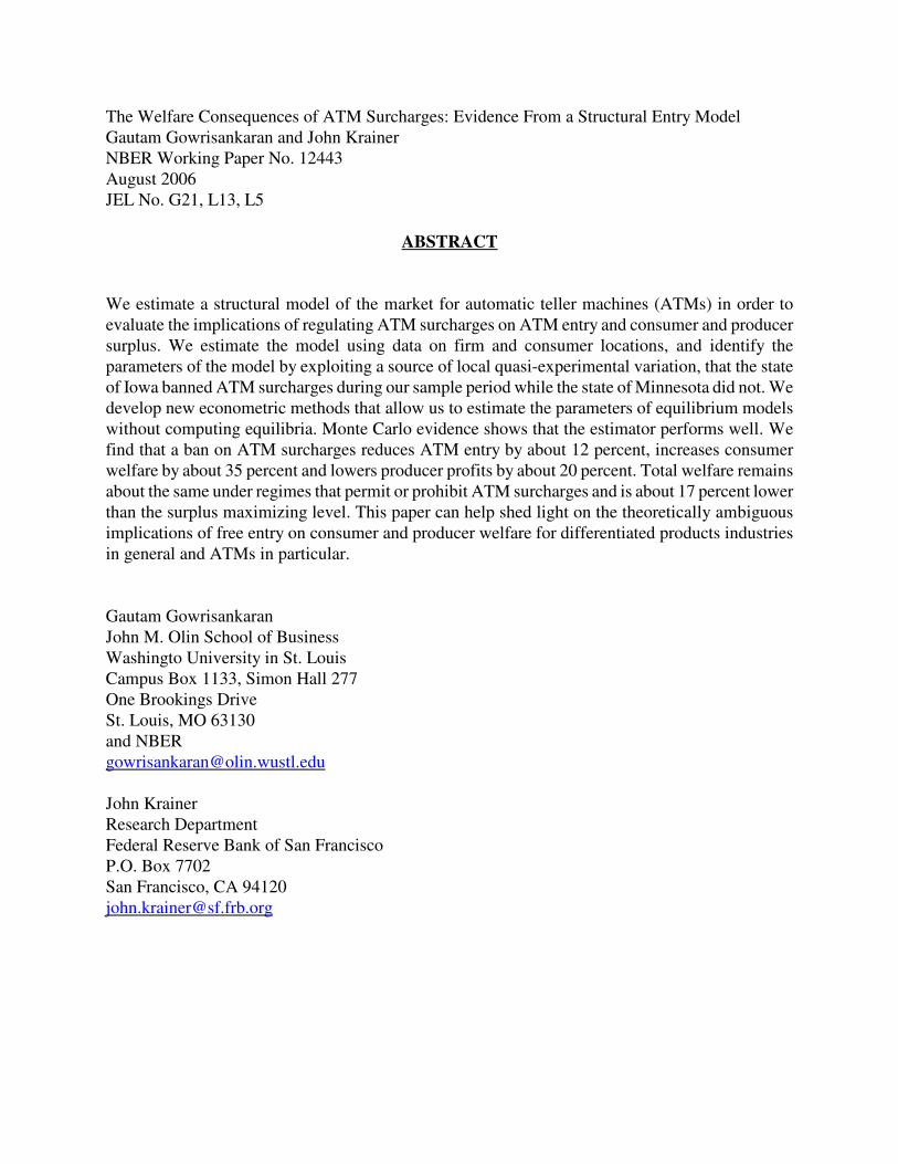
The Welfare Consequences of ATM Surcharges: Evidence From a Structural Entry ModelGautam Gowrisankaran and John KrainerNBER Working Paper No. 12443August 2006JEL No. G21, L13, L5

ABSTRACT

We estimate a structural model of the market for automatic teller machines (ATMs) in order toevaluate the implications of regulating ATM surcharges on ATM entry and consumer and producersurplus. We estimate the model using data on firm and consumer locations, and identify theparameters of the model by exploiting a source of local quasi-experimental variation, that the stateof Iowa banned ATM surcharges during our sample period while the state of Minnesota did not. Wedevelop new econometric methods that allow us to estimate the parameters of equilibrium modelswithout computing equilibria. Monte Carlo evidence shows that the estimator performs well. Wefind that a ban on ATM surcharges reduces ATM entry by about 12 percent, increases consumerwelfare by about 35 percent and lowers producer profits by about 20 percent. Total welfare remainsabout the same under regimes that permit or prohibit ATM surcharges and is about 17 percent lowerthan the surplus maximizing level. This paper can help shed light on the theoretically ambiguousimplications of free entry on consumer and producer welfare for differentiated products industriesin general and ATMs in particular.

Gautam GowrisankaranJohn M. Olin School of BusinessWashingto University in St. LouisCampus Box 1133, Simon Hall 277One Brookings DriveSt. Louis, MO 63130and NBERgowrisankaran@olin.wustl.edu

John KrainerResearch DepartmentFederal Reserve Bank of San FranciscoP.O. Box 7702San Francisco, CA 94120john.krainer@sf.frb.org

2

1. Introduction

The goal of this paper is to estimate a structural model of the market for automatic teller

machines (ATMs) in order to understand the implications of regulating ATM surcharges on

ATM entry and consumer welfare. We develop new econometric methods that allow us to

feasibly estimate the parameters of a structural equilibrium model using entry data without

computing equilibria. This paper can help shed light on the theoretically ambiguous implications

of free entry for consumer and producer welfare for differentiated products industries in general

and ATMs in particular.

Since the establishment of the first ATM networks in the early 1970s, ATMs have

become a ubiquitous and growing component of consumer banking technology. By 2001, there

were over 324,000 ATMs in the United States, processing an average of 117 transactions per

day, suggesting that each person in the United States uses an ATM an average of 45 times per

year.1

In spite of the vast and growing presence of ATMs, product differentiation may imply

that the market for ATMs does not reflect perfect competition or yield optimal outcomes. In

particular, the surcharge—the price charged by an ATM on top of the set interchange fee—has

increased significantly over the last several years. The increase can be linked to an April 1996

decision by the major ATM networks to allow surcharges among their member ATMs.2 Between

1996 and 2001, the number of ATMs tripled, but the number of transactions per ATM fell by

about 45 percent. The technology of ATMs is characterized by high fixed costs—primarily the

1 ATM & Debit News (2001). 2 The decision was made in apparent reaction to the threat of costly antitrust litigation.

3

cost of leasing the machine, keeping it stocked with cash, and servicing it—and very low

marginal costs. Thus, the increased price of ATM services has been accompanied by an

increased average cost per ATM transaction.

The increase in price suggests that there may have been “excess” entry of ATMs, in the

sense that total welfare would have been higher with less entry. It also suggests that a policy by

an ATM network or government that regulated or eliminated surcharges could potentially

increase total welfare. This would likely be true if new ATMs stole significant business from

existing ATMs without sufficiently adding to consumer welfare. However, ATMs are

differentiated products, with a primary characteristic being their location. The increase in the

number of ATMs implies that consumers have to travel less distance to use an ATM. This

decrease in distance can compensate for the increase in price. Therefore, it is theoretically

ambiguous whether price restrictions would increase or decrease welfare. The answer depends

on the relative weight of price and distance in the consumer utility function, firm cost structures,

and the nature of the equilibrium interactions between the agents in the economy.

We address these questions by specifying a static discrete choice differentiated products

model of the ATM market. Consumer utility for an ATM is a function of distance and price.

Firms face a fixed cost per ATM that can vary by location, but no marginal costs. Entry

decisions and prices are determined in a simultaneous–moves Nash equilibrium. We create a data

set that provides detailed locations for actual and potential ATMs and consumers for the border

counties of Iowa and Minnesota. We use the data set together with new econometric techniques

to estimate the structural parameters of the model. We then use our estimated parameters to

assess the equilibrium implications of a surcharge ban and other policies.

4

In general, it might be difficult to identify separately the two effects of distance and price

elasticities using only entry data. However, we are able to identify and estimate these parameters

by using the fact that the state of Iowa banned ATM surcharges during our sample period.3 The

fixed prices in Iowa will identify the distance disutility and firm cost parameters. The fact that

Iowa did not allow surcharges but its neighboring states allowed them creates a source of local

quasi–experimental variation, whereby the different pattern of ATM penetration rates between

places in Iowa near its borders and places just outside the borders of Iowa will identify the price

elasticity of demand.4

This study builds on an entry literature started by Bresnahan and Reiss (1991) and Berry

(1992). Like more recent papers in this literature (Chernew, Gowrisankaran, and Fendrick

(2002), Mazzeo (2002), and Seim (2002)), we incorporate detailed geographic and product data

that allows us to obtain more realistic results. Two other literatures also bear on this work. First

is a literature has estimated spatial models in order to understand the prevalence of excess entry

(see Davis (2002) and Berry and Waldfogel (1999)).

Second, a recent literature has sought to understand the implications of ATM surcharges

(see Croft and Spencer (2003), Hannan, Kiser, McAndrews, and Prager (2004), Ishii (2005),

Knittel and Stango (2004), and Massoud and Bernhardt (2002)). Ishii (2005) and Knittel and

Stango (2004) also try to understand the extent to which consumers value additional ATMs. In

both papers, the authors specify structural models of demand for banks with the main dependent

variable being bank market shares. Our approach has both advantages and disadvantages relative

3 The surcharge ban was overturned by the U.S. Court of Appeals for the Eighth Circuit in 2002. Conversations with industry participants did not lead us to suspect that there was any significant entry in Iowa in anticipation of the repeal of the ban.

5

to these papers. The disadvantage of our approach is that we do not explicitly model the linkage

between the provision of ATM services and other banking services. However, our approach

yields advantages in terms of being able to identify the relevant parameters and predict

equilibrium outcomes. In particular, our identification of price elasticity comes from the

difference in adoption in counties on either side of the Iowa and Minnesota border; the

identification in Knittel and Stango (2004) comes from variation over time in adoption rates,

while the identification in Ishii (2005) is from the cross-sectional variation in bank market shares

within Massachusetts during one year. We explicitly model consumer and ATM locations, and

use this to identify the disutility from travel distance; the other papers use counts of ATMs. Last,

we explicitly model and estimate the structural parameters underlying a bank or ATM decision to

open an ATM, which allows us to simulate the equilibrium impact of a change in the surcharge

policy; the other papers focus only on consumer preferences.

Our model is methodologically most similar to Seim (2002). As in that paper, we assume

that firms operating within a market have incomplete information, in that firms do not know their

competitors’ cost shocks. We also specify the precise location of potential firm entry points

within a localized area. A model of localized competition is crucial for understanding the welfare

impact of ATM surcharges because of the consumers’ tradeoff between location and price. Our

model and estimation strategy differs from and extends Seim’s methodology in three important

ways. First, we model entry as an explicit function of fundamental utility and cost parameters

and then use these parameters to evaluate well–defined policy experiments. In contrast, it is not

possible to obtain fundamental utility parameters from Seim’s work. Second, as noted above, we

4 Other studies that have identified economic parameters using the quasi–experimental variation created by sharp borders between different policy regimes include Holmes (1998), Chay and Greenstone (2003) and Hahn, Todd, and van der Klaauw (2001).

6

identify the price elasticity using the source of quasi–experimental variation created by the

policy differences between Iowa and Minnesota. Third, as necessitated by the complexity of our

model, we develop new econometric methods that allow us to estimate the parameters without

solving for the equilibria of the game, thereby reducing the computational burden of estimating

the model. Our method builds on methods developed by Aguirregabiria and Mira (2002), Guerre,

Perrigne, and Vuong (2000), Hotz and Miller (1993) and Pakes, Ostrovsky, and Berry (2004) in

other contexts.

The remainder of this paper is divided as follows. Section 2 describes the model and

inference. Section 3 details the data, including background on the industry and some reduced–

form evidence. Section 4 provides the results of the estimation and the policy experiments,

including Monte Carlo evidence on the performance of our estimator. Section 5 concludes.

2. Model and Inference

2.1 Model and equilibrium

We develop a simple game–theoretic model of firm and consumer behavior in the market

for ATMs that we estimate using data on consumer locations and potential and actual ATM

locations. The unit of observation is a county for some specifications and the entire border region

of a state for other specifications. Our model is static. We feel that a static model is a reasonable

approximation since sunk costs in the ATM industry are low; machines can be resold, and ATMs

are generally installed within existing retail establishments.

7

There exists a set of potential ATM locations j = 1,…, J , each with an entrepreneur. Each

entrepreneur simultaneously decides whether to install an ATM at her location.5 In Minnesota,

each entrepreneur also chooses her price (conditional on entry) at the same time as the entry

decision. Our model of firms abstracts away from the strategic effect of firms with multiple

ATMs, as most merchants do not have multiple retail establishments within the same immediate

geographic area.

Consumers, denoted i = 1,…, I , observe the set of actual ATMs as well as the posted price

for each ATM. In Iowa, these prices are fixed at zero, although the regulated price that the ATM

receives from the transaction (which is called the interchange fee) is positive. Consumers then

make a decision of which ATM to use, if any.

There are several simplifications inherent in our specification that are necessitated by the

lack of available consumer data. First, we do not model the fact that consumers may not know

the prices or locations of all ATMs, and hence that there may be a search. In addition, we model

ATM transactions as a separate good, rather than as part of a menu of banking services. Thus, we

do not model the fact that the consumer’s bank may charge a fee in addition to the fee charged

by the ATM, nor do we allow for banks to price discriminate by not surcharging their own

banking customers, or to subsidize ATM transactions as a way of obtaining customers and

charging them for other services.6 To check the robustness of this latter assumption, we report

results where we restrict the sample to include only nonbank ATM locations (i.e., convenience

5 Note that this model is different from Seim (2002) in that her model assumes that each video store entrepreneur chooses one census tract from the set of tracts in the county. The difference in approaches stems from the fact that we believe that existing retail establishments are a reasonable universe for the set of potential ATM locations, while the set of potential video store locations is more open. 6 See Massoud and Bernhardt (2002).

8

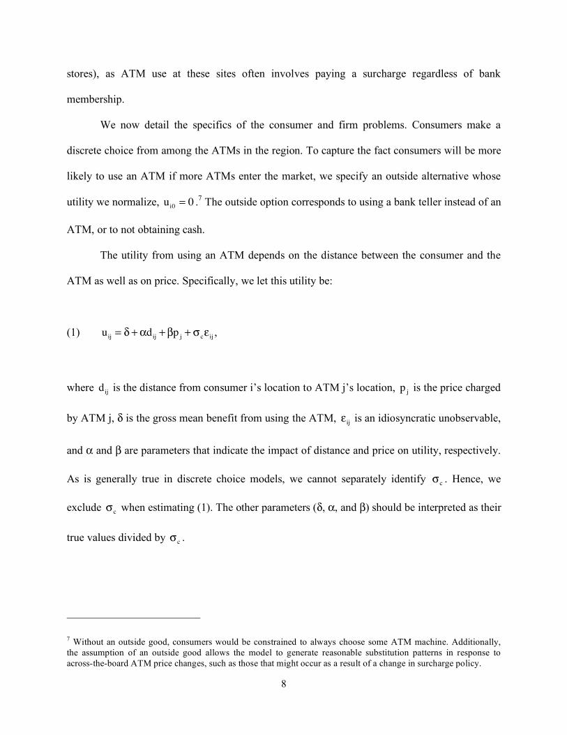
stores), as ATM use at these sites often involves paying a surcharge regardless of bank

membership.

We now detail the specifics of the consumer and firm problems. Consumers make a

discrete choice from among the ATMs in the region. To capture the fact consumers will be more

likely to use an ATM if more ATMs enter the market, we specify an outside alternative whose

utility we normalize, ui0= 0 .7 The outside option corresponds to using a bank teller instead of an

ATM, or to not obtaining cash.

The utility from using an ATM depends on the distance between the consumer and the

ATM as well as on price. Specifically, we let this utility be:

(1) uij = ! +"dij +#p j + $c%ij ,

where dij is the distance from consumer i’s location to ATM j’s location, p j is the price charged

by ATM j, δ is the gross mean benefit from using the ATM, !ij is an idiosyncratic unobservable,

and α and β are parameters that indicate the impact of distance and price on utility, respectively.

As is generally true in discrete choice models, we cannot separately identify !c. Hence, we

exclude !c when estimating (1). The other parameters (δ, α, and β) should be interpreted as their

true values divided by !c.

7 Without an outside good, consumers would be constrained to always choose some ATM machine. Additionally, the assumption of an outside good allows the model to generate reasonable substitution patterns in response to across-the-board ATM price changes, such as those that might occur as a result of a change in surcharge policy.

9

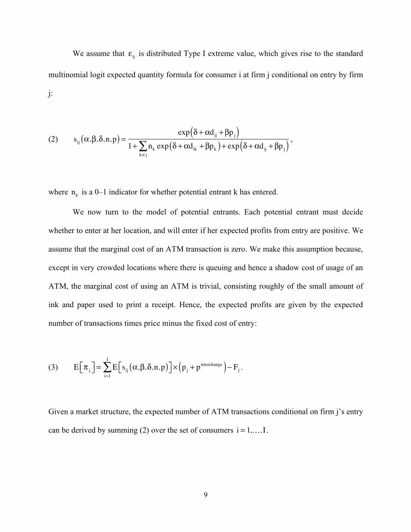
We assume that !ij is distributed Type I extreme value, which gives rise to the standard

multinomial logit expected quantity formula for consumer i at firm j conditional on entry by firm

j:

(2) sij !,",#,n,p( ) =exp # +!dij +"p j( )

1+ nkk$ j

% exp # +!dik +"pk( ) + exp # +!dij +"p j( ),

where nk is a 0–1 indicator for whether potential entrant k has entered.

We now turn to the model of potential entrants. Each potential entrant must decide

whether to enter at her location, and will enter if her expected profits from entry are positive. We

assume that the marginal cost of an ATM transaction is zero. We make this assumption because,

except in very crowded locations where there is queuing and hence a shadow cost of usage of an

ATM, the marginal cost of using an ATM is trivial, consisting roughly of the small amount of

ink and paper used to print a receipt. Hence, the expected profits are given by the expected

number of transactions times price minus the fixed cost of entry:

(3) E ! j"# $% = E sij &,',(,n,p( )"# $%

i=1

I

) * p j + pinterchange( )+ Fj .

Given a market structure, the expected number of ATM transactions conditional on firm j’s entry

can be derived by summing (2) over the set of consumers i = 1,…, I .

10

In contrast to marginal costs, the fixed costs of ATMs are high, about $1,300 per month,8

and might differ by location. We model fixed costs as:

(4) Fj = c j + !ee j with c j = ! county j + "! atbank j ,

where c j is observable to all potential ATMs in the region, and can be divided into a fixed effect

that is specific to a small group of counties ( ! county j ) and a shifter for whether the ATM is located

at a bank ( !" atbank j ) as opposed to at another retail establishment such as a grocery store.

We let e j be distributed logit (i.e., as the difference of two i.i.d. Type 1 extreme value

random variables), with a standard deviation !e. We assume that e j is known to firm j at the

time of her entry decision. However, we assume that firm j does not know the fixed cost shocks

for the other potential entrants. The use of unobservable cost shocks of this type is common in

the entry literature,9 as it helps reduce the number of equilibria for entry models.

The incomplete information about the cost shocks implies that it is meaningful to

consider a Bayesian–Nash equilibrium (BNE). In Iowa, a BNE specifies the entry decision for

each type e j for each firm, j = 1,…, J . It is easy to show that any BNE is characterized by a

vector of cutoffs e1,…, e

J, whereby firm j will enter if and only if e j ! ej . Let the 0-1 indicator

in j denote whether firm j enters or not, and let Pr in j ej( ) denote the entry (or no entry)

probability for firm j before e j is realized. The logit assumption implies that the density of in j

8 See Dove Consulting (2004). 9 See, for instance, Seim (2002) and Augereau, Greenstein and Rysman (2002).

11

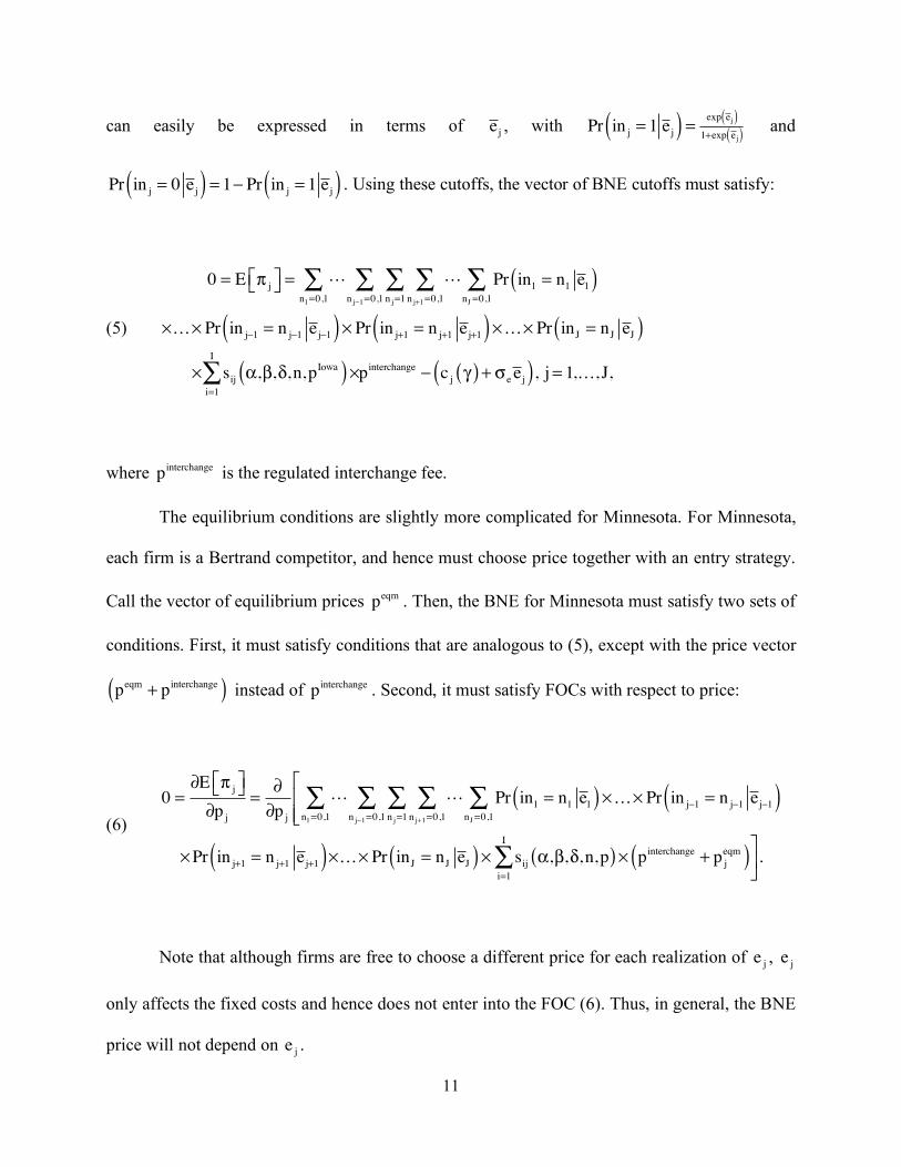
can easily be expressed in terms of ej , with Pr in j = 1 ej( ) = exp ej( )1+exp ej( )

and

Pr in j = 0 ej( ) = 1! Pr in j = 1 ej( ) . Using these cutoffs, the vector of BNE cutoffs must satisfy:

(5)

0 = E ! j"# $% = ! ! Pr in1 = n1 e1( )

nJ =0,1

&n j+1=0,1

&n j=1

&n j'1=0,1

&n1=0,1

&

(…( Pr in j'1 = n j'1 ej'1( )( Pr in j+1 = n j+1 ej+1( )(…( Pr inJ = nJ eJ( )

( sij ),*,+,n,pIowa( )(

i=1

I

& pinterchange ' c j ,( ) + -e ej( ), j = 1,…, J,

where pinterchange is the regulated interchange fee.

The equilibrium conditions are slightly more complicated for Minnesota. For Minnesota,

each firm is a Bertrand competitor, and hence must choose price together with an entry strategy.

Call the vector of equilibrium prices peqm . Then, the BNE for Minnesota must satisfy two sets of

conditions. First, it must satisfy conditions that are analogous to (5), except with the price vector

peqm + pinterchange( ) instead of pinterchange . Second, it must satisfy FOCs with respect to price:

(6)

0 =!E " j

#$ %&!p j

=!!p j

! ! Pr in1 = n1 e1( )nJ =0,1

'n j+1=0,1

'n j=1

'n j(1=0,1

'n1=0,1

' )…) Pr in j(1 = n j(1 ej(1( )#

$**

)Pr in j+1 = n j+1 ej+1( ))…) Pr inJ = nJ eJ( )) sij +,,,-,n,p( )) pinterchange + p jeqm( )

i=1

I

' %

&. .

Note that although firms are free to choose a different price for each realization of e j , e j

only affects the fixed costs and hence does not enter into the FOC (6). Thus, in general, the BNE

price will not depend on e j .

12

2.2 Estimation

The predictions of the model specified in Section 2.1 depend on structural parameters that

specify consumer utility and firm costs, which we group together as ! = ",#,$, % ,&e( ) . Our goal

is to obtain consistent estimates of the true parameters !0, and use the estimates to evaluate the

impact of ATM surcharges on welfare and ATM entry.

We could potentially obtain consistent and asymptotically efficient estimates of !0 using

the method of maximum likelihood. For a given θ, the likelihood is a function of endogenous

data on entry and exogenous data on consumer locations, potential entrant firm locations, and the

surcharge regime (e.g., Iowa or Minnesota). Let y j denote a 0–1 indicator for whether firm j has

entered, and x denote the exogenous data for the region. If we assume that there is a unique

vector of equilibrium cutoffs for any given θ and x, then we can write the log likelihood for the

region as:

(7) lnL y j,!( ) = ln Pr in j = y j ej !,x( )( )( )j=1

J

" ,

where the equilibrium cutoffs are calculated using the appropriate FOCs (5) and/or (6) depending

on the state and where we have now made explicit their dependence on x and θ.

In principle, we could estimate θ by maximizing the log likelihood function (7), as in

Seim (2002). However, maximizing (7) would require computing the equilibrium entry

probabilities for each parameter vector. Unlike Seim (2002), the equilibrium entry behavior in

13

our model depends on an aggregation of individual consumer’s utility–maximizing decisions and

on a pricing equilibrium, which makes this process computationally intractable for our model.

We develop an alternative method of inference that allows us to find consistent estimates

of θ without explicitly solving for the BNE. Our method exploits the observation that a firm’s

optimal decisions depend on the equilibrium actions of other firms only through the distribution

of other firms’ actions. If all the information that a firm has about this distribution is also

observable to the econometrician, then one can solve for the optimal behavior of firms,

conditional on structural parameters, by substituting the distribution of the other firms’ actions

from the data. This then allows us to create a pseudo-likelihood for any vector of structural

parameters.

This same idea has been used to develop estimators for a variety of different models.

Hotz and Miller (1993) develop methods to estimate the parameters of dynamic optimization

problems without evaluating the dynamic decision problems, using the fact that decisions in the

data reflect optimal behavior at the true parameters. In Hotz and Miller’s case, the analog of the

econometrician observing all the known characteristics of a firm’s rivals is that there are no

unobservable serially correlated state variables. Guerre, Perrigne, and Vuong (2000) develop

methods to estimate the structural parameters of first–price private–value auctions without

solving for the BNE of the auction game, based on the fact that an agent’s optimal bid depends

on others’ values solely through their bids, and that these bids are observable to the

econometrician. Aguirregabiria and Mira (2002), Bajari, Benkard and Levin (2005), and Pakes,

Ostrovsky, and Berry (2004) show how to apply these methods to Markov–perfect equilibrium

games. The common feature in all of these methods is that they rely on substituting the

distribution of actions of other individuals (or one’s future self in the case of Hotz and Miller

14

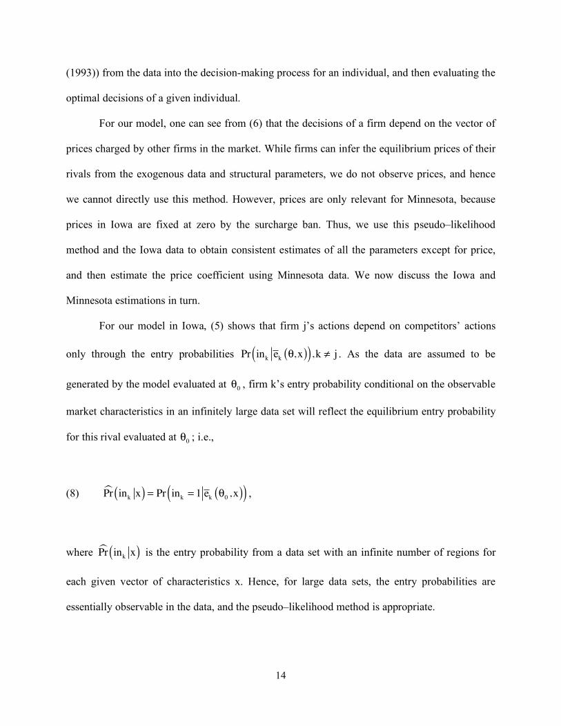
(1993)) from the data into the decision-making process for an individual, and then evaluating the

optimal decisions of a given individual.

For our model, one can see from (6) that the decisions of a firm depend on the vector of

prices charged by other firms in the market. While firms can infer the equilibrium prices of their

rivals from the exogenous data and structural parameters, we do not observe prices, and hence

we cannot directly use this method. However, prices are only relevant for Minnesota, because

prices in Iowa are fixed at zero by the surcharge ban. Thus, we use this pseudo–likelihood

method and the Iowa data to obtain consistent estimates of all the parameters except for price,

and then estimate the price coefficient using Minnesota data. We now discuss the Iowa and

Minnesota estimations in turn.

For our model in Iowa, (5) shows that firm j’s actions depend on competitors’ actions

only through the entry probabilities Pr ink ek !,x( )( ),k " j . As the data are assumed to be

generated by the model evaluated at !0, firm k’s entry probability conditional on the observable

market characteristics in an infinitely large data set will reflect the equilibrium entry probability

for this rival evaluated at !0; i.e.,

(8) Pr! in

kx( ) = Pr ink = 1 ek !

0,x( )( ) ,

where Pr! in

kx( ) is the entry probability from a data set with an infinite number of regions for

each given vector of characteristics x. Hence, for large data sets, the entry probabilities are

essentially observable in the data, and the pseudo–likelihood method is appropriate.

15

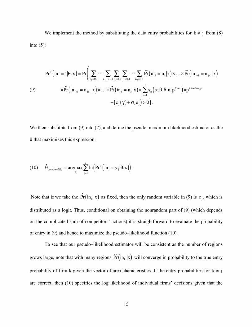
We implement the method by substituting the data entry probabilities for k ! j from (8)

into (5):

(9)

Prd in j = 1 !,x( ) = Pr ! ! Pr" in1 = n1 x( )nJ =0,1

"n j+1=0,1

"n j=1

"n j#1=0,1

"n1=0,1

" $…$%

&' Pr" in j#1 = n j#1 x( )

$Pr" in j+1 = n j+1 x( )$…$ Pr" inJ = nJ x( )$ sij (,),*,n,pIowa( )$

i=1

I

" pinterchange

# c j +( ) + ,ee j( ) > 0).

We then substitute from (9) into (7), and define the pseudo–maximum likelihood estimator as the

θ that maximizes this expression:

(10) !pseudo"ML = argmax!

ln Prd in j = y j !,x( )( )j=1

J

# .

Note that if we take the Pr! in

kx( ) as fixed, then the only random variable in (9) is e j , which is

distributed as a logit. Thus, conditional on obtaining the nonrandom part of (9) (which depends

on the complicated sum of competitors’ actions) it is straightforward to evaluate the probability

of entry in (9) and hence to maximize the pseudo–likelihood function (10).

To see that our pseudo–likelihood estimator will be consistent as the number of regions

grows large, note that with many regions Pr! in

kx( ) will converge in probability to the true entry

probability of firm k given the vector of area characteristics. If the entry probabilities for k ! j

are correct, then (10) specifies the log likelihood of individual firms’ decisions given that the

16

firms’ beliefs about their competitors are governed by !0. Thus, !pseudo"ML will approach the

maximum likelihood estimator of this individual firm problem. Standard asymptotic theory

implies that this individual firm maximum likelihood problem will provide consistent estimates

of θ, and hence !pseudo"ML will also be consistent. Section 4, which provides Monte Carlo

evidence on the performance of our estimator relative to the maximum likelihood estimator

based on (7), shows that the pseudo–likelihood and maximum–likelihood estimators perform

very similarly.

There are a few important details of this estimator that we have not yet discussed. First is

the computation of the entry probabilities from the data, Pr! in

kx( ) . We perform a reduced–form

logit estimation of entry on all exogenous data x, and then use the predicted values as Pr! in

kx( ) .

In an infinitely large data set, we could nonparametrically estimate Pr! in

kx( ) by including a

nonparametric expansion of x in the logit estimation. With finite data, the dimensionality of the

characteristics space is too large. We include in this reduced–form logit estimation the number of

consumers within each of six distance bands (.2, 1, 2, 5, 10, and 20 kilometers), the number of

other potential entrants and potential at–bank (as opposed to at–grocer) entrants within these

same distance bands and interactions of these variables. A central reason to report Monte Carlo

experiments is to examine the extent to which this approximation to the true Pr! in

kx( ) biases

our estimates. Note also that the reduced–form logit model also provides us with a confidence

region for Pr! in

kx( ) . It is straightforward to bootstrap from this confidence region in order to

obtain standard errors for the structural parameters θ that account for this approximation.

17

Second, it is computationally difficult to solve for the nonrandom part of (9), because it

involves a sum over 2J!1 terms, and J, the number of potential ATM locations, has a mean of

about 30 per county in these rural counties. Thus, we evaluate this sum using simulation.

Specifically, we take uniform draws and convert them to a 0–1 realization of entry based on

Pr! in

kx( ) . We estimate our model with 20 simulation draws. As is standard in the literature, we

use the same draws across different parameter values. We experimented with using more

simulation draws but found almost no change in the pseudo–likelihood. The Monte Carlo

experiments confirm that the simulations do not substantially change the estimates.

Third, we maximize the pseudo–likelihood function using the derivative–based Newton

method. We did not experience any convergence problems, probably because the function is

similar to a logit. We compute standard errors for the parameter estimates using the standard

approximation based on the sum of the outer–product of the derivatives of the individual

contributions to the log likelihood.

Fourth, in some specifications, we estimate the entire border region in Iowa jointly,

instead of county by county. We do this to avoid potentially misspecifying the market in cases

where firms and consumers are near the border of two counties. For these specifications, we only

consider the firms and consumers within 50 kilometers of the potential entrant, in order to reduce

computational costs. This approximation is unlikely to affect the results substantially.

We now turn to the estimation of the price coefficient β. We make the identifying

assumptions that fixed costs for border counties in Minnesota are similar to fixed costs for the

corresponding Iowa border counties, and that consumers’ preferences are similar across the two

regions. This implies that, after estimating the Iowa model, the only unknown parameter for the

Minnesota data is β.

18

Although the fact that price is unobservable implies that we cannot directly substitute

competitors’ prices in the same way that we substitute competitors’ entry decisions in Iowa, we

can still directly substitute the entry probabilities from the data for the equilibrium entry

probabilities, as we do for Iowa. After doing this, (6) becomes

(11)

0 =!!p j

! ! Pr" in1 = n1 x( )nJ =0,1

"n j+1=0,1

"n j=1

"n j#1=0,1

"n1=0,1

" $…$ Pr" in j#1 = n j#1 x( )$%

&''

Pr" in j+1 = n j+1 x( )$…$ Pr" inJ = nJ x( )$ sij (,), *,n,p( )$ pinterchange + p jeqm( )

i=1

I

" +

,- , j = 1,…, J,

where !, "( ) are the estimated values of the parameters from the Iowa data. We solve for the

vector peqm by simultaneously solving the FOCs in (11). We then define the probability of entry

analogously to (9) as:

(12)

Pr in j = 1!,x( ) =

Pr ! ! Pr" in1 = n1 x( )nJ =0,1

"n j+1=0,1

"n j=1

"n j#1=0,1

"n1=0,1

" $…$ Pr" in j#1 = n j#1 x( )$%

&' Pr" in j+1 = n j+1 x( )

$…$ Pr" inJ = nJ x( )$ sij (,!, ),n,peqm( )

i=1

I

" $ peqm + pinterchange( )# c j *( ) + +ee j( ) > 0,-.,

where ! , "e( ) are also estimated values of the parameters from the Iowa data. We then define the

pseudo–likelihood estimator as the β that maximizes the analogous expression to (10) with the

substitution of the correct entry probability from (12).

19

Our substitution of the reduced–form entry probabilities simplifies the equilibrium

computation, since we do not have to solve for the entry probabilities. As with the Iowa data, we

evaluate (11) and (12) using simulation. Even with simulation methods and the substitution for

the exogenous entry probabilities, evaluating the likelihood for Minnesota is very

computationally intensive. However, our overall computation time is lessened because we only

have to estimate one parameter with this method.

Importantly, the reduced–form relationship between the entry probability and exogenous

variables will be different in Minnesota than in Iowa, because of the difference in the nature of

competition. However, the exogenous observable data remain the same. Hence, we estimate

different reduced–form coefficients for Minnesota but use the same reduced–form model as for

Iowa.

One potential issue is the possibility of multiple equilibria. Multiple equilibria are

particularly likely when the standard deviation of the idiosyncratic components of profits, !e, is

small. For instance, with small !e, if there are two entrants at a given location, then it may be

profitable for exactly one entrant to enter, but not for both. This source of multiple equilibria is

common in entry models.10 Multiple equilibria are less likely in our model when there are sizable

unobservable idiosyncratic components of profits. Moreover, one additional advantage of our

estimation strategy is that it is robust to multiple equilibria if the equilibrium selection conditions

on observables. As an example, if it is always the case that the equilibrium entry selection

specifies that firms enter in order of most to least profitable based on observable variables, then a

sufficiently rich reduced–form model will capture this equilibrium behavior. However, our

model is not robust to sunspot equilibria, since no predictor of probabilities based on observables

20

can generate equilibrium selection based on unobservables. Note that our counterfactual policy

experiments will not be robust to the presence of multiple equilibria.

2.3 Identification

Our data is quite different from the data commonly used to identify consumer preferences

for discrete choice utility specifications. For instance, we lack data on prices (except for the

interchange fees) and quantities that is commonly used to estimate discrete choice models.

Instead, we have data on locations and entry decisions and different policy regimes.11 Since it is

not immediately apparent how these data identify the parameters, we discuss this issue.

Recall that we estimate all of our parameters except for the coefficient on price using the

Iowa data. Thus, it is necessary that the Iowa data identify the consumer disutility of distance

α and mean utility δ, and the means γj and standard deviation σe of the fixed costs of entry.

These parameters will be identified from variations across markets in the number of potential

entrants, the number of consumers, and the relative distances between these sets.

In particular, the model is semiparametrically identified: with enough data, we can

recover the parameters and the underlying distribution of the fixed costs of entry without

imposing a parametric functional form on the fixed costs of entry. To see this, fix δ, and consider

a sequence of markets (e.g. separate counties) which all have exactly one potential entrant, but

vary continuously in the number of consumers.12 For now, assume also that all consumers are

located at the same place as the firm, so that distance is irrelevant. Given δ, we can evaluate the

10 See, for instance, Berry (1992) and Andrews and Berry (2002). 11 Recent work by Thomadsen (2005) estimates discrete choice models with price data but without quantity data. While we do not have price data, the crucial information that we do have that discrete choice analyses typically do not have is the set of potential locations that chose not to set up ATMs.

21

marginal profits for any potential entrant as a function of the number of consumers (since the

revenue per customer is pinterchange , which is known). By tabulating the fraction of actual entrants

for any number of consumers, we can recover the distribution of fixed costs. As an example,

suppose that when there are 545 consumers, marginal profits are 1.4, and the single potential

entrant enters 73 percent of the time. For the given δ, this implies that the distribution of fixed

costs, which we will call G, satisfies G

!1.73( ) = 1.4 . With enough variation across the number of

consumers, we can recover the entire distribution of fixed costs.

Different values of δ will imply different substitution patterns from the outside good to an

ATM as the number of firms increases. With a high δ, total transactions will remain roughly

constant; with a lower δ, total transactions will increase, as more people substitute from the

outside good. Intuitively then, δ will be identified from the differences in entry patterns across

the number of firms. The Appendix formally proves that with infinite data, the only value of δ

that will yield the same G distribution across 1 or 2 potential entrants is the true δ. Hence, the

model is identified using data with different numbers of potential entrants, as there is only one

possible candidate for the estimate of δ, namely the one that yields the same G distribution

across potential entrants.

Since we have non-parametrically recovered the whole distribution of fixed costs, the

parameters on mean fixed costs γ will be identified from the mean of the distributions of fixed

costs for banks and grocery stores. With sufficient data, we can identify any distribution for e

with mean zero.

12 In the actual data, the number of consumers can only vary discretely. But since the variation in distance is

22

The disutility of distance parameter α can be identified from variation in the distances

between consumers and potential entrants across markets. For example, with a very negative α,

there will be much less entry if otherwise identical consumers and firms are far away from each

other. With α close to zero, this variation in the data will have little effect.

Last, the consumer parameter on disutility of price will be identified from the different

pattern of entry in Minnesota from Iowa. For example, if demand is very elastic, then firms will

be unable to obtain high surcharges from consumers in Minnesota, and hence the number of

ATMs per capita should be similar in the two regions. If demand is inelastic, however, we should

see more ATMs in Minnesota. In addition, if demand is inelastic, the pattern of entry will be

different in Minnesota, with less clustering in the town centers as margins from entry will fall

with more firms.

While the above arguments show that we can obtain identification with data from an

infinite number of markets, as a practical matter, we only have data from the Iowa and

Minnesota border counties. Thus, it is of interest to understand how much our actual data can

identify. In Section 4.1 we perform Monte Carlo experiments that show the precision of

estimates given our exogenous data on firm and consumer locations.

continuous, this is not a limitation.

23

3. Data

3.1 The ATM industry

The ATM industry infrastructure consists of card issuing banks, ATM machines, and a

telecommunications network to process transactions.13 In the early stages of ATM deployment,

ATM machines were generally owned and operated by banks, with the machines physically

located on the bank premises. By the 1990s, much of the growth in ATM deployment shifted to

nonbank locations, such as convenience stores and grocery stores.14 Today, the majority of

ATMs are located at sites other than banks. More than 75 percent of all ATM transactions are

cash withdrawals, with the remainder being deposits and balance inquiries.

ATM cardholding customers, ATMs, and card issuing banks are all linked together by

shared networks. In 2002, there were about 40 networks, the largest being the national networks

of Cirrus and Plus, which are owned by MasterCard and Visa, respectively.15 A transaction

involving a customer from Bank A using an ATM owned by Institution B generates a number of

fees. Bank A must pay the network a switch fee for routing the transaction. These fees range

from 3 to 8 cents per transaction.16 Second, Bank A, the card issuing bank, must pay the ATM

owner, Institution B, an interchange fee. These fees range from 30 to 40 cents for a withdrawal

and are determined by the ATM network. In the case where an ATM and a customer’s bank both

use multiple networks, the actual interchange fee will vary based upon the agreements between

the ATM and the different networks. Bank A may also charge its cardholding customer a foreign

13 Hayashi, Sullivan, and Weiner (2003) provide a detailed background on the industry. 14 According to a recent survey by Dove Consulting (2004), the most attractive sites for new entry are convenience stores, shopping malls, supermarkets, airports, and schools. 15 See Hayashi, Sullivan, and Weiner (2003). 16 See Hayashi, Sullivan, and Weiner (2003).

24

fee for using Institution B’s machine; we do not model this fee. Institution B may charge the

customer a surcharge fee for using its ATM machine. As of 2002, 87 percent of all ATM

deployers levied surcharges on foreign-acquired customers. The average surcharge across all

operators was about $1.50. However, fees are typically only paid by about one-third of

customers,17 suggesting a mean actual fee of 50 cents.

According to a recent consulting study, the average ATM cost $1,314 per month to

operate in 2003, with the costs consisting mostly of fixed items such as depreciation,

maintenance, telecommunications, and cash replenishment.18 Revenue comes from the assorted

fees generated by an ATM transaction.

3.2 Sample and data

Our first data choice is in defining the sample. As our model is identified by the

difference in the pattern of ATM diffusion for Iowa and Minnesota, we want the Iowa and

Minnesota counties in our sample to have similar consumer preferences and firm costs. To

ensure that we have similar counties, we keep the border counties from each state as well as

counties that are within one county of the border. Eight of the counties in the eastern part of

Minnesota have more population density than the corresponding Iowa counties and include

medium-sized cities such as Rochester. We believe that the dense counties are sufficiently

different from the corresponding Iowa counties, and so we exclude these counties from our

sample. Figure 1 displays a map of the counties in our sample, and their population densities.19

17 See Dove Consulting (2002). 18 See Dove Consulting (2004). 19 The banking markets in the Iowa and Minnesota counties considered here are also similar. In 2002, the market share of the ten largest banking institutions operating in the 21 Iowa counties was 32%, versus 47% in the 11

25

We create three principal sources of data for the counties in our sample: potential ATM

locations, actual ATM locations, and consumer locations. Our data come from the year 2002,

prior to the lifting of the surcharge ban in Iowa. We discuss each of these data sources in turn.

Our first data set provides the set of potential ATM locations. ATMs are almost certain to

be inside other retail establishments, particularly in the rural counties from our sample. We

obtained phone numbers of all the retail establishments for one county in Iowa (Mitchell

County), using the web site switchboard.com. By calling every retail establishment in that

county, we found that the ATMs were all located in grocery stores (including convenience

stores) or banks. Based on this initial query, we chose grocery stores and banks as the set of

potential ATMs. We obtained the addresses and phone numbers of grocery stores and banks for

our counties from a private company called InfoUSA, which markets this information for

commercial use. We then geocoded these addresses to obtain detailed latitude and longitude

information.

Our second data source is information on the locations of ATMs. We obtained location

data from several large ATM networks with substantial operations in Minnesota and Iowa. The

networks in our data set include Visa Plus, a network that is national in scope, and SHAZAM,

which is based in Iowa and has ATMs throughout the central states.20 The data provide the

addresses of ATMs for all machines in the databases of the networks. In the case of Visa Plus,

the database is used for their web-based ATM finder.

There are two potential problems with these data: missing ATMs and missing potential

ATMs. We found that the ATM locator databases were incomplete, resulting in many missing

Minnesota counties. Both markets are considered unconcentrated. The Herfindahl-Hirschman Index was 188 for the counties in Iowa and 314 for the counties in Minnesota in 2002. 20 We thank these networks for providing us with data.

26

ATMs. To address this problem, we called every InfoUSA potential entrant (i.e., grocery stores,

and banks) and asked if there was an ATM on the premises. For Iowa, this process resulted in the

identification of an additional 93 entrants from the telephone interviews (24 percent of the total

number of entrants). For Minnesota, we identified an additional 105 entrants from the telephone

interviews (52 percent of the total).

The InfoUSA data of potential ATMs was more complete, though still not perfect. About

25 percent of the entrants from the ATM locator databases were not in the InfoUSA database.

These missing ATMs were distributed fairly evenly, accounting for about 10 percent of our total

sample in each state. Of the missing 98 ATMs, 38 were located in grocery stores and

convenience stores and 26 were located in banks that were simply not in the InfoUSA list. The

others were in specialized categories, such as colleges, hospitals, and movie theaters.

Our third data set provides the locations for consumers. These data are from the 1990

Census, and provide the location of consumer residences at the census block level. This level is

not quite as fine as the address level, but still very small. It would be possible to supplement

these data with data on employment locations, treating these as additional people, although this

would likely have little effect, because of the similarity of residential and employment locations

in our sample of rural counties.

For some of our estimates, we allow the entire border region to have the same mean fixed

costs for ATMs. For other estimates, we allow the mean fixed costs to vary across counties. For

these estimates, we group the mean fixed costs so that the Iowa border county, its southern

neighbor (e.g., Lyon and Sioux, respectively) and its Minnesota neighbors (Pipestone and Rock,

in this case) all share the same fixed costs. Note that firms compete exclusively within a county

27

in our base specifications and with everyone in the whole border region of their state for other

specifications.

In the estimation we assume that the interchange fee, pinterchange , is 35 cents, an

approximation to true values noted above. The value of pinterchange will not affect the coefficient

estimates in the Iowa analysis, as expected profits in (5) are proportional to pinterchange . However,

the chosen value will affect coefficient estimates in Minnesota because, with surcharging,

expected profits are now proportional to the sum of the interchange fee and the entering firm’s

price.

3.3 Reduced-form evidence

Table 1 provides some summary statistics of the data. We have 32 counties in our data, of

which 21 are in Iowa. Our counties are sparsely populated, with an average of about 16,000

people per county in Iowa, and somewhat fewer in Minnesota. In spite of the relatively small

populations in this region of the country, each county contains about 1,000 census blocks,

suggesting that the unit of geographic measurement for people is small. There are, on average,

about 15 percent fewer potential ATM locations in Minnesota than in Iowa. The number of

actual and potential ATMs varies a lot across counties, from a low of 10 to a high of 87.

In Iowa, there are an average of 18.8 ATMs per county and 1.13 ATMs per 1000 people

per county. The corresponding statistics for Minnesota are 18.3 and 1.23, suggesting that the

unregulated price may result in more entry. We can sharpen this intuition with a county-level

regression of ATMs per person on a state dummy variable, including controls for the number of

consumers and potential entry locations, shown in Table 2.

28

Table 2 reports that Iowa counties have about 20 percent fewer ATMs than Minnesota

counties with similar characteristics, compared to the 8 percent difference in the raw data

reported in Table 1. The greater difference compared to Table 1 is explained by the fact that the

Iowa counties have more potential ATM locations, which appears to cause more entry. Both

Tables 1 and 2 show that most of the difference between ATM deployment in Minnesota and

Iowa is attributable to additional deployment at grocery stores and not at banks. This is probably

because banks are installing ATMs at their branches for reasons other than generating transaction

fees, such as diverting customers away from more costly transactions with a bank teller.

In addition to predicting more entry in Minnesota, our model also predicts a different

pattern of entry. In particular, entrants in Minnesota should be more likely to stay away from

other potential entrants, in order to exercise more local monopoly power. The last row of Table 2

examines whether this prediction is substantiated in the data. We find that ATMs in Iowa are

more likely to be near other potential ATMs, as predicted in the data.

Figure 2 shows the potential and actual ATM locations and population for two

neighboring counties, Osceola County, Iowa, and Nobles County, Minnesota. These two counties

contain a mix of both small towns (e.g., Worthington, MN, and Sibley, IA) and rural areas. One

can see that entry is more likely in the urban areas than in outlying areas. In addition, consistent

with Table 2, there is more entry in rural areas in Minnesota than in Iowa. Last, note that there

are some potential ATMs near the county borders, for instance in Brewster, MN, suggesting that

it might be important to allow competition to extend beyond the county border.

4. Results

29

4.1 Monte Carlo evidence

Before examining parameter estimates from actual data, we provide Monte Carlo

evidence on the performance of our estimator. We construct simulated data by choosing “true”

parameters and exogenous data, computing equilibrium entry probabilities conditional on these

values, and then simulating entry decisions from the equilibrium entry probabilities. As with the

real data, we construct “Iowa” data where prices are regulated to be zero, and “Minnesota” data

where prices can vary. We repeat the simulation 10 times to create 10 independent data sets, and

then examine the performance of different estimators across the 10 data sets.

The Monte Carlo evidence is presented in Table 3. Column 1 provides the parameter

values that we used to simulate the data. We chose the parameters to be round numbers that are

close to both our initial priors and the estimated parameters.

Columns 2–4 describe three different sets of parameter estimates, all based on the same

simulated data sets. The data sets for these columns have 500 distinct markets, with 10 or fewer

firms and 50 or fewer consumer locations per market. These sizes are chosen to ensure that the

maximum likelihood estimator is computationally feasible, which is not true for the real data.

Column 2 describes the maximum likelihood estimates computed using (7), column 3 describes

the pseudo–likelihood estimates where the sums are completely evaluated instead of simulated,

and column 4 describes the simulated pseudo–likelihood estimates; these use the same estimator

that we use to estimate the model with the real data. Each entry in the table lists the mean and

standard deviation of the estimated parameters across the 10 data sets (and not the standard

errors of the estimates).

As with the real data, we estimate every parameter but the price coefficient β using the

“Iowa” data. We can then potentially use these estimated parameters and the “Minnesota” data to

30

estimate the price coefficient. We did not include these results because of the prohibitive

computational cost of performing the 40 maximum likelihood estimation runs (10 each for

columns 2–5) necessary to generate this Monte Carlo evidence. However, we did perform the

“Minnesota” estimation for a more limited number of runs. While we do not report these results,

the findings are consistent with the Monte Carlo evidence that we report.

We find that all three estimators perform similarly and well. For instance, the true value

of α, the disutility of distance, is –.25, and the mean estimated values for the three methods are

all within .005 of the true value, with standard deviations of less than .07. Moreover, the

differences between the true parameters and the mean estimated parameters are likely due to the

fact that we have only simulated 10 data sets (for computational reasons). Thus, columns 2–4

demonstrate that our model is well–identified given the simulated data, and that the pseudo-

likelihood method appears to yield little loss in efficiency relative to the method of maximum

likelihood.

A remaining question is the extent to which our actual data contain enough variation to

identify the parameters well. Column 5 of Table 3 describes the estimated parameters for data

sets where the exogenous data are the real data and the endogenous data are computed using the

equilibrium and the values of the true parameters reported in column 1. Again, the pseudo–

likelihood estimator performs well. This suggests that our real exogenous data contain enough

variation to identify the parameters, provided that the endogenous data are generated by the

model.

Also of interest is the performance of our reduced–form predictors of the entry

probabilities, which are used in the pseudo–likelihood estimation. Since we know the true

probabilities of entry for the simulated data from the equilibrium computation, we can compare

31

the true probabilities to the predicted probabilities. The bottom row of Table 3 lists the mean root

mean squared differences in the probabilities for the Iowa and Minnesota estimation for the two

data sets. We find a fairly close match between the two, with mean root mean squared

differences of about .06 for the first data set and somewhat larger values of .125 to .192 for the

second data set, probably because of the smaller sizes in this case. This further suggests that our

reduced–form approximations of the true entry probabilities are reasonable.

4.2 Parameter estimates

We turn now to our base parameter estimates for the real data, which are given in Table

4. The specifications for this table assume that customers and ATMs only compete with other

customers and banks within the same county. There are two sets of specifications: in column 1

the mean fixed cost is assumed to be the same across counties, while column 2 allows fixed costs

to vary by county, as discussed in Section 3. For each specification, the first several rows provide

the parameters that are estimated from Iowa data, while the price coefficients at the bottom are

estimated from the Minnesota data.

The model with different fixed costs across counties fits the Iowa data better, in the sense

that a likelihood ratio test could reject the fact that the fixed costs are the same across counties

(!2 10( ) = 21.6 , p=.02). For the Minnesota data, it is not possible to conduct a likelihood ratio

test, since the parameter values for the other parameters are not the same. Nonetheless, column 1

has a lower likelihood, suggesting that the fixed costs from neighboring Iowa counties are not

fitting the Minnesota data as well as the mean fixed costs across counties.

Most of the estimates in this table are precisely estimated and appear to be reasonable.

The coefficient of distance on utility is –.178 in column 1 and –.151 in column 2. The coefficient

32

in column 2, but not column 1, is significantly different from zero at traditional significance

levels. This implies that a person who had a 50 percent chance of using a particular ATM would

use it with roughly 46 percent probability if the ATM were to move 1 kilometer further away.

This coefficient appears to be a reasonable tradeoff of distance for a sample that consists of rural

Iowa and Minnesota.

The coefficient on price is estimated to be –1.48 in column 1 and –2.18 in column 2. This

implies that a consumer values one kilometer of distance as 8 cents to 10 cents depending on the

specification, figures that also appear to be reasonable. The estimates also imply that a person

who had a 50 percent chance of using a particular ATM would use it with 46 percent probability

(column 1) or 45 percent (column 2) if price were to increase by 10 cents. This suggests that

consumers are quite price elastic. The underlying reason why our estimates of the price elasticity

are high is because, in the data, ATM entry per capita is only slightly higher in Minnesota than in

Iowa. This suggests that firms are not able to make much more money in Minnesota, which in

turn implies that demand is elastic.

From column 1, the mean fixed costs of operating an ATM at a nonbank location is

estimated to be $93 with a standard deviation of $263. For column 2, the mean fixed costs are

estimated to vary between $19 and $409, with a standard deviation of $153.

The mean fixed costs of operating an ATM at a bank is estimated to be almost exactly the

same. We initially found it surprising that banks would not have a lower fixed cost of entry than

grocers. However, the raw data show a very similar entry probability for banks and grocers (58

percent vs. 62 percent), which explains this finding.

As our consumer model is a discrete choice, the time period in our model of roughly one

week is the interval over which consumers might decide whether or not to make a cash

33

withdrawal. Our estimates of fixed costs for actual entrants are smaller but reasonably close to

the (imputed) weekly fixed costs of about $300 noted in Section 3. The smaller estimates are

likely due to grocery stores and banks opening ATMs because of complementarities.

Table 5 provides a set of alternate specifications as a robustness check. The first

specification allows for competition across the entire border region within a state. We report a

specification that imposes the same mean fixed costs across counties, though we found similar

results when the fixed costs are allowed to vary across counties. The parameter estimates are

very similar to those from Table 4 Model 1. In particular, the coefficients on distance are

estimated to be slightly larger in magnitude (–.275 instead of –.178). The coefficients on price

are similar, as are the coefficients on fixed costs.

One potential issue with our model is that we have simplified the profit function for

potential ATMs to ignore the complementarity with their other business. This is potentially more

problematic for banks, who may install ATMs mostly as a convenience to their banking

customers, rather than to earn the ATM fees. The second specification provides a model where

we model the entry decisions for non-banks (principally grocery stores) only. In this

specification, we assume that entry decisions for banks are exogenously made, and fixed at their

actual value. This specification yields similar results to the base specification, suggesting that

grocery stores and banks are choosing to open ATMs based on roughly the same criteria. One

issue is that our coefficients mostly lose their significance, likely because the sample size is

effectively smaller, since it now includes only the non-banks as potential entrants.

Table 6 provides predictions of the estimated model, including the equilibrium prices and

quantities for ATMs, which are useful for understanding the fit of our model. We predict that the

average surcharge is 38 cents when surcharges are allowed. This is about one-third the mean

34

posted surcharge. However, since only one-third of customers actually pay the surcharge, it is as

close as the model can come to reflecting reality, given that we do not allow firms to charge

surcharges selectively in our model.21 The average number of ATM transactions is about 555 for

every 1,000 people per week when surcharges are banned, with about a 20 percent decrease to

469 transactions when surcharges are allowed. Dividing these figures by the number of ATMs

per 1,000 people, we find that each ATM is performing about 500 transactions per week when

surcharges are allowed and 400 when they are not, numbers that are very consistent with industry

data.22 These figures suggest that our model is able to replicate key equilibrium predictions of the

model reasonably well, in spite of the fact that the parameters are estimated using only entry

data.

4.3 Counterfactual policy experiments

Table 6 uses the parameter estimates to evaluate the impact of counterfactual surcharge

policies on consumer and firm welfare and the prevalence and price of ATMs. We do this by

postulating counterfactual policy regimes and simulating the equilibrium entry decisions given

these policy regimes. We examine both bans and taxes on surcharges. For any vector of firm

entry decisions, we can evaluate the expected consumer welfare and firm profits using the

standard multinomial logit formulas. The consumer welfare measures are in units of utility.

However, we can convert them to dollars by dividing them by the estimated marginal utility of

21 As a robustness check, we estimate a specification where two-thirds of consumers do not pay the surcharge and one-third do pay the surcharge. This specification results in an estimated average price of $2.80, somewhat higher than the mean posted surcharge. 22 Dove Consulting (2002) reports an average of 4,479 transactions per month per on-premise machine and 1,560 per month per off-premise machine.

35

money, which is !" . This then allows us to add consumer and producer surplus to form a

measure of total surplus.

We can also compute the policy that maximizes total surplus, as would be chosen by a

social planner with this goal. We assume that the planner provides a mandatory entry and pricing

strategy to each firm as a function of that firm’s cost draw, but does not coordinate entry

decisions across firms. As the marginal cost of an ATM transaction is zero, the planner will

always pick prices of zero, leaving only the entry decision to be computed.

Table 6 provides the results of these counterfactual experiments, evaluated using the

parameters of Table 4, Model 1. We chose to use a specification where the mean fixed costs are

the same across counties because of its fit to the Minnesota data.

Under both the surcharge and no surcharge regimes, the average total surplus per 1,000

people is about $885, with a standard deviation of about $230. Even though there is almost no

difference in the mean total welfare levels between the two regimes, allowing for surcharges has

large distributional consequences. A ban on surcharges increases consumer surplus by about 33

percent (from $333 to $446 per 1,000 people) and reduces producer surplus by about 20 percent.

Not surprisingly, allowing for surcharges results in more ATMs (an average of 1.27 instead of

1.12 per 1,000 people) but fewer total transactions due to the higher prices. The implication is

that consumers gain more from the lower prices without surcharges than they do from the lower

travel time when surcharges are allowed. However, firms are not able to capture as much of the

surplus with just the fixed interchange fee, and hence, they lose out.

We also considered a regime where surcharges are allowed, but where firms must pay a

20 percent tax on the surcharges that is remitted to consumers on a lump–sum basis. This regime

results in outcomes that are between the two boundary cases. Consumer and producer surpluses

36

are both in between the two extreme policies. In addition, the mean surcharge with the tax is

about 20 percent lower than if the surcharges are unregulated.

All three regimes result in a welfare level that is about 14 percent lower than the planner

welfare level. The planner chooses about 50 percent more ATMs than even under the surcharge

regime. The fact that there is more entry implies that firms are adding to consumer surplus with

their entry more than they are reducing profits to other firms by stealing their business. Because

of the additional entry and the zero prices, the volume of transactions is higher than under the

other regimes.

One of the surprising results from the policy experiments is the finding that surcharge

bans depress ATM entry by just 12 percent. This relatively small effect stands in stark contrast to

the observation that ATM deployment tripled between 1996 (when the networks lifted their

surcharge ban) and 2001 but is completely consistent with the difference between Iowa and

Minnesota border data. It is worth noting that ATM deployment was growing rapidly throughout

the 1980s and early 1990s as well, apparently for reasons other than the price of ATM services.

For this reason, we believe that our border study affords the cleanest way of identifying the

relationship between surcharges and entry.

5. Conclusion

We have developed a structural model of ATM utility, costs, and entry. Our specification

of utility includes travel distance and price. We assume that potential entrant firms enter based

on the total revenues from entering minus the fixed costs; we assume that marginal costs are

zero. We also assume that a firm’s fixed cost is private information that is not revealed to other

37

firms in the industry. Firms’ entry decisions are based on the Bayesian–Nash equilibrium of their

entry game.

We develop a quasi–likelihood method to estimate the parameters of this model using

data on the locations of consumers, potential ATMs, and actual ATMs. Our method of inference

obtains estimates of our game–theoretic model of entry without solving for the equilibrium of the

game, and hence is computationally feasible. Our estimation procedure is identified by the fact

that the state of Iowa fixed the surcharge price of ATMs at zero during our sample period. This

allows us to estimate most of the parameters from Iowa data, without worrying about the price

elasticity. We then make the assumption that consumer preferences and costs for counties in

Minnesota and Iowa near their border are similar. By substituting the parameters estimated using

Iowa data, we then recover the price elasticity using the Minnesota data.

We provide Monte Carlo evidence on our estimation procedure, and find that the quasi–

likelihood method yields similar results to the method of maximum likelihood and can provide

reasonably precise estimates given the scope of our data. Turning to the results, we find a

coefficient on distance that is significantly negative and moderate in size. The consumer tradeoff

between price and distance also fits our expectations. We use these estimates to find the welfare

and entry consequences of an ATM surcharge ban. We find that a surcharge ban would

moderately decrease the number of ATMs, increase consumer surplus, decrease firm profits, and

result in roughly the same total surplus. Mean total welfare levels are quite similar across

regimes that allow surcharges and regimes that ban them. However, the choice of surcharge

regime has large distributional consequences. A surcharge ban raises consumer welfare by about

35 percent, while lowering producer welfare by about 20 percent. Policies that allow surcharges

38

and policies that totally ban them, result in welfare levels that are about 17 percent below the

first–best welfare levels.

We believe that our study results in three principal outputs. First, it provides evidence on

the impact of ATM surcharges on outcomes and surplus levels in the market for ATMs. More

generally, this provides evidence on the nature of excess entry in other differentiated products

oligopoly markets. Since our study is cross sectional in nature, our methods are less susceptible

to the problem of confounding entry due to the lifting of the surcharge ban with entry due to

whatever exogenous factors have caused ATM deployment to flourish since the early 1980s.

Second, it shows that data on firm entry combined with quasi–experimental variation in policies

can be used to estimate the demand and cost parameters of this industry. Third, the study shows

that our quasi–likelihood method can be used to feasibly estimate the parameters of structural

game theoretic models without solving for the equilibria of the games.

Appendix

As discussed in Section 2.3, with infinite data we can uniquely recover the distribution of fixed

costs for any number of potential entrants n, conditional on δ. Call the recovered distribution

G

n,! and let

!

0 denote the true δ.

Proposition:

Assume that there are infinite data for 1 and 2 potential entrants and for each value of the number

of consumers. Then, G

1,!= G

2,!" ! = !

0.

Proof:

39

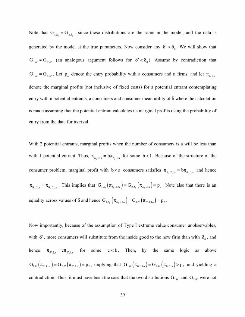
Note that G

1,!0

= G2,!

0

, since these distributions are the same in the model, and the data is

generated by the model at the true parameters. Now consider any !" > "

0. We will show that

G

1, !"# G

2, !" (an analogous argument follows for

!" < "

0). Assume by contradiction that

G

1, !"= G

2, !". Let

p

n denote the entry probability with a consumers and n firms, and let

!

" ,n,a

denote the marginal profits (not inclusive of fixed costs) for a potential entrant contemplating

entry with n potential entrants, a consumers and consumer mean utility of δ where the calculation

is made assuming that the potential entrant calculates its marginal profits using the probability of

entry from the data for its rival.

With 2 potential entrants, marginal profits when the number of consumers is a will be less than

with 1 potential entrant. Thus, !

"0

,2,a= b!

"0

,1,a for some b < 1. Because of the structure of the

consumer problem, marginal profit with b ! a consumers satisfies !

"0

,2,ba= b!

"0

,1,a and hence

!

"0

,2,a= !

"0

,2,ba. This implies that G1,!0

"!0 ,1,ba( ) = G2,!0

"!0 ,2,a( ) = p2 . Note also that there is an

equality across values of δ and hence G1,!0"

!0 ,1,ba( ) = G1, #!"

#! ,1,ba( ) = p2 .

Now importantly, because of the assumption of Type I extreme value consumer unobservables,

with !" , more consumers will substitute from the inside good to the new firm than with !

0, and

hence !

"# ,2,a= c!

"# ,1,a for some c < b . Then, by the same logic as above

G1, !" #!" ,1,ca( ) = G2, !" #

!" ,2,a( ) = p2 , implying that G1, !" #!" ,1,ba( ) = G2, !" #

!" ,2,a( ) > p2 and yielding a

contradiction. Thus, it must have been the case that the two distributions G1, !"

and G2, !"

were not

40

identical. Last, note that although we have assumed that consumer unobservables follow a Type I

extreme value distribution, the proof would work with any distribution that results in substitution

away from the outside good as the number of firms increases.

References Aguirregabiria, Victor and Pedro Mira (2002). “Identification and Estimation of Dynamics

Discrete Games.” Mimeo, Boston University. Andrews, Donald W. K. and Steven Berry (2002). “On Placing Bounds on Parameters of Entry

Games in the Presence of Multiple Equilibria.” Mimeo, Yale University. Augereau, Angelique, Shane Greenstein, and Marc Rysman (2002). “Coordination vs.

Differentiation in a Standards War: 56K Modem Adoption by ISP's.” Mimeo, Boston University.

ATM & Debit News (2001). Available on the world wide web at

http://www.cardforum.com/html/atmdebnews/atmlinks.htm. Bajari, Patrick, Lanier Benkard and Jonathan Levin (2005). “Estimating Dynamic Models of

Imperfect Competition.” Mimeo, Stanford University. Berry, Steven (1992). “Estimation of a Model of Entry in the Airline Industry”. Econometrica

60(4) 889 – 917. Berry, Steven and Joel Waldfogel (1999). “Free Entry and Social Inefficiency in Radio

Broadcasting.” RAND Journal of Economics 30: 397–420. Bresnahan, T. and P. Reiss (1991). “Entry and Competition in Concentrated Markets.” Journal of

Political Economy 99: 977–1009. Card, David and Alan B. Krueger (1994). “Minimum Wages and Employment: A Case of the

Fast–Food Industry in New Jersey and Pennsylvania.” American Economic Review 84: 772–793.

Chay, Kenneth and Michael Greenstone (2003). “The Impact of Air Pollution on Infant

Mortality: Evidence from Geographic Variation in Pollution Shocks Induced by a Recession.” Quarterly Journal of Economics 118: 1121–1167.

Chernew, Michael, Gautam Gowrisankaran and A. Mark Fendrick (2002). “Payer Type and the

Returns to Bypass Surgery: Evidence from Hospital Entry Behavior,” Journal of Health Economics 21: 451 – 474.

41

Croft, E., and B. Spencer (2003). “Fees and surcharging in automatic teller machine networks:

no–bank ATM providers versus large banks.” Mimeo, Sauder School of Business, UBC. Davis, P. (2002). “Entry, Cannibalization and Bankruptcy in the U.S. Motion Picture Exhibition

Market.” Mimeo, London School of Economics. Dove Consulting (2002). “2002 ATM Deployer Study.” Available on the web at

http://www.pulse-eft.com/upload/Deployer_2002_executive.pdf. Dove Consulting (2004). “New ATM Study Details a Paradoxical Industry.” Available on the web

at http://www.doveconsulting.com/PR-2004-05-21CPPS.htm. Guerre, E., I. Perrigne and Q. Vuong (2000). “Optimal Nonparametric Estimation of First–Price

Auctions.” Econometrica 68: 525–74. Hahn, Jinyong, Petra Todd, and Wilbert Van der Klaauw (2001). “Identification and Estimation

of Treatment Effects with a Regression–Discontinuity Design.” Econometrica 69: 201–9. Hannan, T., E. Kiser, J. McAndrews, and R. Prager (2004). “To Surcharge or Not to Surcharge:

An Empirical Investigation of ATM Pricing.” Forthcoming, Review of Economics and Statistics.

Hayashi F., R. Sullivan and S.E. Weiner (2003). A Guide to the ATM and Debit Card Industry.

Kansas City, MO: Federal Reserve Bank of Kansas City. Holmes, Thomas J. (1998). “The Effect of State Policies on the Location of Manufacturing:

Evidence from State Borders.” Journal of Political Economy 106: 667–705. Hotz, V. Joseph V. and Robert A. Miller (1993). “Conditional Choice Probabilities and the

Estimation of Dynamic Models.” Review of Economic Studies 60: 497–529. Ishii, J. (2005). “Interconnection Pricing and Compatibility in Network Industries: ATM

Networks in the Banking Industry.” Mimeo, Harvard University. Knittel, C., and V. Stango (2004). “Compatibility and Pricing with Indirect Network Effects:

Evidence from ATMs.” Mimeo, University of California, Davis. Massoud, N., and D. Bernhardt (2002). “Rip–off ATM Surcharges.” RAND Journal of

Economics, 33(1), 96–115. Mazzeo, Michael (2002). “Product Choice and Oligopoly Market Structure,” RAND Journal of

Economics 33: 1–22. Pakes, Ariel, Michael Ostrovsky and Steven Berry (2004). “Simple Estimators for the

Parameters of Discrete Dynamic Games (with Entry / Exit Examples).” Mimeo, Harvard

42

University. Seim, Katja (2002). “An Empirical Model of Firm Entry with Endogenous Product–Type

Choices.” Mimeo, Stanford University Graduate School of Business. Thomadsen, Raphael (2005). ““The Effect of Ownership Structure on Prices in Geographically

Differentiated Industries,” Forthcoming, RAND Journal of Economics.

43

Table 1:

Summary statistics of the data by county and state

Statistic Mean Std. Dev. Min Max N

Potential ATM locations 32.6 16.5 14 87 21

ATMs 18.8 10.9 5 48 21

ATMs per 1000 consumers 1.13 .347 .458 2.08 21

ATMs not at banks per 1000 consumers .688 .263 .092 1.27 21

Consumers 16,384 8,720 7,267 46,733 21

Iow

a co

untie

s

Census blocks with consumers 988.1 315.8 563 1,727 21

Potential ATM locations 27.7 8.16 17 42 11

ATMs 18.3 5.90 10 30 11

ATMs per 1000 consumers 1.23 .188 .960 1.48 11

ATMs not at banks per 1000 consumers .789 .159 .498 1.01 11

Consumers 15,021 4,910 9,660 22,914 11

Min

neso

ta c

ount

ies

Census blocks with consumers 944.7 271.3 582 1,407 11

44

Table 2: Reduced–form determinants of ATM entry

OLS regressions at county level

Regressors

Iowa Consu-mers

(1000s)

Potential entry

locations

Potential grocer entry

locations

Potential bank entry locations

Adjusted R2 Obs.

ATMs per 1000

consumer

–.256*** (.073)

–.111*** (.016)

.063*** (.008) .62 32

Bank ATMs per 1000 cons.

–.057 (.044)

–.043*** (.010)

.013 (.009) .031**

(.014) .49 32

Grocer ATMs per 1000 cons.

–.207*** (.073)

–.073*** (.017)

.009 (.015)

.050** (.024) .37 32

Logit estimation at potential ATM level

Regressors

Iowa Nearby pot. ATMs

Nearby consumers

(1000s)

Nearby pot. ATMs ! Iowa

Nearby cons. !

Iowa

Log likelihood Obs.

Entry –.107 (.250)

–.102 (.094)

4.54** (2.00)

.242** (.110)

–5.97*** (2.28) –655.2 989

Note: Standard errors in parentheses. All regressions include a constant term. “Nearby” refers to within .2 kilometers. *** Significant at 1% level ** Significant at 5% level

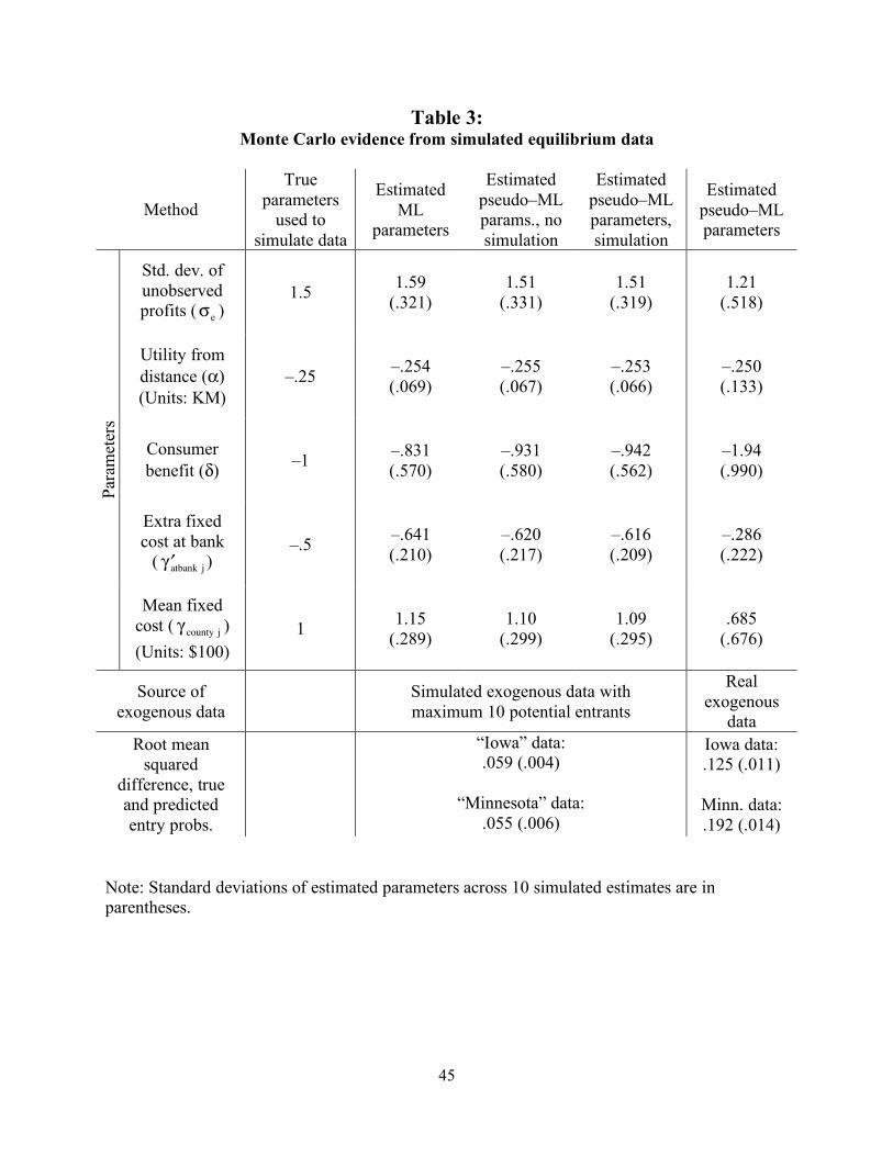
45

Table 3: Monte Carlo evidence from simulated equilibrium data

Method

True parameters

used to simulate data

Estimated ML

parameters

Estimated pseudo–ML params., no simulation

Estimated pseudo–ML parameters, simulation

Estimated pseudo–ML parameters

Std. dev. of unobserved profits (!

e)

1.5 1.59 (.321)

1.51 (.331)

1.51 (.319)

1.21 (.518)

Utility from distance (α) (Units: KM)

–.25 –.254 (.069)

–.255 (.067)

–.253 (.066)

–.250 (.133)

Consumer benefit (δ) –1 –.831

(.570) –.931 (.580)

–.942 (.562)

–1.94 (.990)

Extra fixed cost at bank

( !" atbank j ) –.5 –.641

(.210) –.620 (.217)

–.616 (.209)

–.286 (.222)

Para

met

ers

Mean fixed cost ( ! county j ) (Units: $100)

1 1.15 (.289)

1.10 (.299)

1.09 (.295)

.685 (.676)

Source of exogenous data Simulated exogenous data with

maximum 10 potential entrants

Real exogenous

data Root mean

squared difference, true and predicted entry probs.

“Iowa” data: .059 (.004)

“Minnesota” data:

.055 (.006)

Iowa data: .125 (.011)

Minn. data: .192 (.014)

Note: Standard deviations of estimated parameters across 10 simulated estimates are in parentheses.

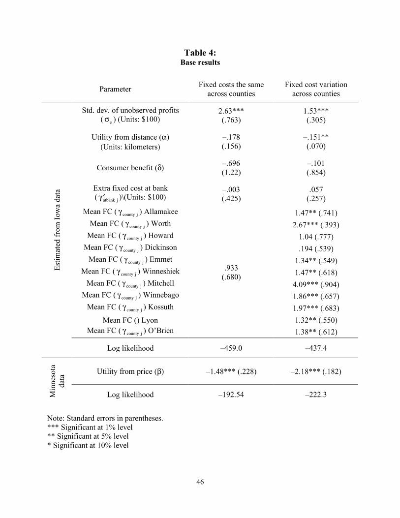
46

Table 4: Base results

Parameter Fixed costs the same across counties

Fixed cost variation across counties

Std. dev. of unobserved profits (!

e) (Units: $100)

2.63*** (.763)

1.53*** (.305)

Utility from distance (α) (Units: kilometers)

–.178 (.156)

–.151** (.070)

Consumer benefit (δ) –.696 (1.22)

–.101 (.854)

Extra fixed cost at bank ( !" atbank j )\(Units: $100)

–.003 (.425)

.057 (.257)

Mean FC ( ! county j ) Allamakee 1.47** (.741) Mean FC ( ! county j ) Worth 2.67*** (.393)

Mean FC ( ! county j ) Howard 1.04 (.777) Mean FC ( ! county j ) Dickinson .194 (.539)

Mean FC ( ! county j ) Emmet 1.34** (.549) Mean FC ( ! county j ) Winneshiek 1.47** (.618)

Mean FC ( ! county j ) Mitchell 4.09*** (.904) Mean FC ( ! county j ) Winnebago 1.86*** (.657)

Mean FC ( ! county j ) Kossuth 1.97*** (.683) Mean FC () Lyon 1.32** (.550)

Mean FC ( ! county j ) O’Brien

.933 (.680)

1.38** (.612)

Estim

ated

from

Iow

a da

ta

Log likelihood –459.0 –437.4

Utility from price (β) –1.48*** (.228) –2.18*** (.182)

Min

neso

ta

data

Log likelihood –192.54 –222.3

Note: Standard errors in parentheses. *** Significant at 1% level ** Significant at 5% level * Significant at 10% level

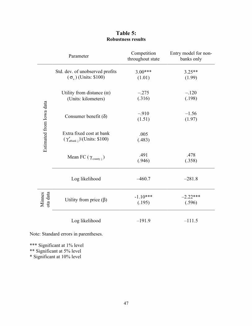
47

Table 5: Robustness results

Parameter Competition throughout state

Entry model for non-banks only

Std. dev. of unobserved profits (!

e) (Units: $100)

3.00*** (1.01)

3.25** (1.99)

Utility from distance (α) (Units: kilometers)

–.275 (.316)

–.120 (.198)

Consumer benefit (δ) –.910 (1.51)

–1.56 (1.97)

Extra fixed cost at bank ( !" atbank j )\(Units: $100)

.005 (.483)

Mean FC ( ! county j ) .491 (.946)

.478 (.358)

Estim

ated

from

Iow

a da

ta

Log likelihood –460.7 –281.8

Min

nes

ota

data

Utility from price (β) -1.10*** (.195)

–2.22*** (.596)

Log likelihood –191.9 –111.5

Note: Standard errors in parentheses. *** Significant at 1% level ** Significant at 5% level * Significant at 10% level

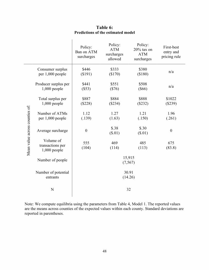
48

Table 6: Predictions of the estimated model

Policy:

Ban on ATM surcharges

Policy: ATM

surcharges allowed

Policy: 20% tax on

ATM surcharges

First-best entry and

pricing rule

Consumer surplus per 1,000 people

$446 ($191)

$333 ($170)

$380 ($180) n/a

Producer surplus per 1,000 people

$441 ($53)

$551 ($76)

$508 ($66) n/a

Total surplus per 1,000 people

$887 ($228)

$884 ($234)

$888 ($232)

$1022 ($239)

Number of ATMs per 1,000 people

1.12 (.139)

1.27 (1.63)

1.21 (.150)

1.96 (.261)

Average surcharge 0 $.38 ($.01)

$.30 ($.01) 0

Volume of transactions per

1,000 people

555 (104)

469 (114)

485 (113)

675 (83.8)

Number of people 15,915 (7,567)

Number of potential entrants

30.91 (14.26)

Mea

n va

lue

acro

ss c

ount

ies o

f:

N 32

Note: We compute equilibria using the parameters from Table 4, Model 1. The reported values are the means across counties of the expected values within each county. Standard deviations are reported in parentheses.

� � � � � � � � � � �

�

� �

� � � � � � �

� � � � �

� � � � � � � � � �

�

! " � � � � # $ % $ & ' ' (

� ) * + , - - . / / / � 0 1 2

�

3

4 4 4 4

�

��

�����

� �� �� �������

���

�

� ������� � � � �� �� �� �

��������� � � ��

���� � � � � �������� ��

� �

� �

�� ���� � ���� � �� �

�

�

�

����� � � ���

������

� � ���

� � � � � � ����� � � � � ������ � �� � ���� �

��������� � � � �� �� �� ������ �

��� � ���

� � � ������

������� �� � � ����� � � �������� � � � �

���� �����

� � � � � ���������� ��� �� �� � �� �� � � �����

��� � �� � � �����

� ��� � � � � �� � �� �� � ����� ��������� � �� � ��� �������� ��� ������� � ��� � � � � � � �� � � �� �� � � ���� ��� � � ���� �� �� �

����� ��� � � � � �� �� ������ � � � ����������� � � � ����� � ������� ����� � � ��

�����������

�

� ��� ���������

�

� ����� � �� ��

���� � � ������ � ��

�� ����

��� ���� ���

������� � � � ����

� �� � �� � � ���� �

���� � � � �� � ��������� � � �� � � � � � ���� � ������ � � ��� ������ � ������������� � ������� � � �� � ���

��

� � � �� ������

������

��������������

�� ������� � ��

� ���

������������� �

� �

���� �

����

����� � ����� � ��� ���� � � �� �� � �� �� � � ������ � � � � ����������� � � � � � � � ������������� � � �� �� � � ��� � �� ����

� �� � � ����� � � ����� � ���

��������� �� ������� ��

��� �� ��

��

����

���� �� ��

������

� � �� � ������ � � � ��

��

��� � �

��

� � �� �� � � ������� �� � ������ ��� �� �� �� � ���� �� �

��

��� ���� � � ������� � � � ������� ���

� � � �� �

��

�� �������

��

������ � �����

������� �� � � ����� � � ����������� �� � � �

� ��� ����� � � � ������� �� �� � ������ � ����� � � �� � �������� ���� � �� � �

���

�

�

�

�

� �������������

��� � � � � � � � �� � ��

� � � � ���� �������� � � � � �������� � � � � � ��������� � ��� �� � � � ��� �

� � � � ��� � �����

�� � � ��

��

���� � �

���

� ������ � � � �������

�

����

�

��

� � � ������ � � � ������ ��

�

�����

�� �

�� � ����

� ������� � � � �����

���

� � � � �����

�� �

� � � � ��

����������� ��� � ��� � � � � � ���������� �� �

�� �

������ ���������

� ����� � � ������� ������

� � � �� �� ���������

� �� � ���������� �

� �

�������� � � � � �������� � � � � ����������� � � � �����

� � � � ����� ����� �

� � ������ � ��� � �

����� �� � � � ����

��

� ����� ��� �� �

� �������� � � � �� ������ �

� � � ����� � ��������

�� ��� ��

�

��� ����

� � � ���������� � � � ���

������

���� �

�� �� ��� � ����� � �� � ������� �� ��

��� ��� � ���� �� �� ���� � ���� � �� �

������� ��

� �� ������� �

��

���

����� ��� � ��� � � ���

������ � � � � ��

�� �

��� ����� �

�� ��

� ��

����

��� � ����� � �� �� ���� �

� ����� ����� � ��� � � ��

�

��

� ���

���� � � � �� ��� �� � ���� � ���� �� �

�������� � � � � � ���������� � � � � ���������� � � � ���

� � �� ������

�� � �������

� � � � ����� � ����� � � � � ��� �� �� � �� ����� ���� �� ����������� � � � ���� � � ��� �������� � � � � � ����������� � � � �� �� �������� �� � � ������� ������ � �� � �� � � � �� ������ �� � � ������ � �� ����� � � �� � ������� ������ � � �� � �� � �� � � � � � ����� �� �� �� ��� ����� � �� ������� � ��� �� �� ������ �� �� ��� � � ���� � � ����� �������� � � ��� �� ��������������� � ���� � ��� ��� �������

������ � ��

��� �� � ��������

� ���� � ��� �

������ ���� ��

��������� �� � ��� �

��

��

�� ��

��

��

��

��

����

��

����

��

��

��

����

����

��

�� ��

���

�

� ��

�

� �� ����

�

���� ��

�

�

�

��� �

� �

�

� �

�

�

� � � � � �

� � � � � �

� � � � � � � �

� ! " # $ % & " %

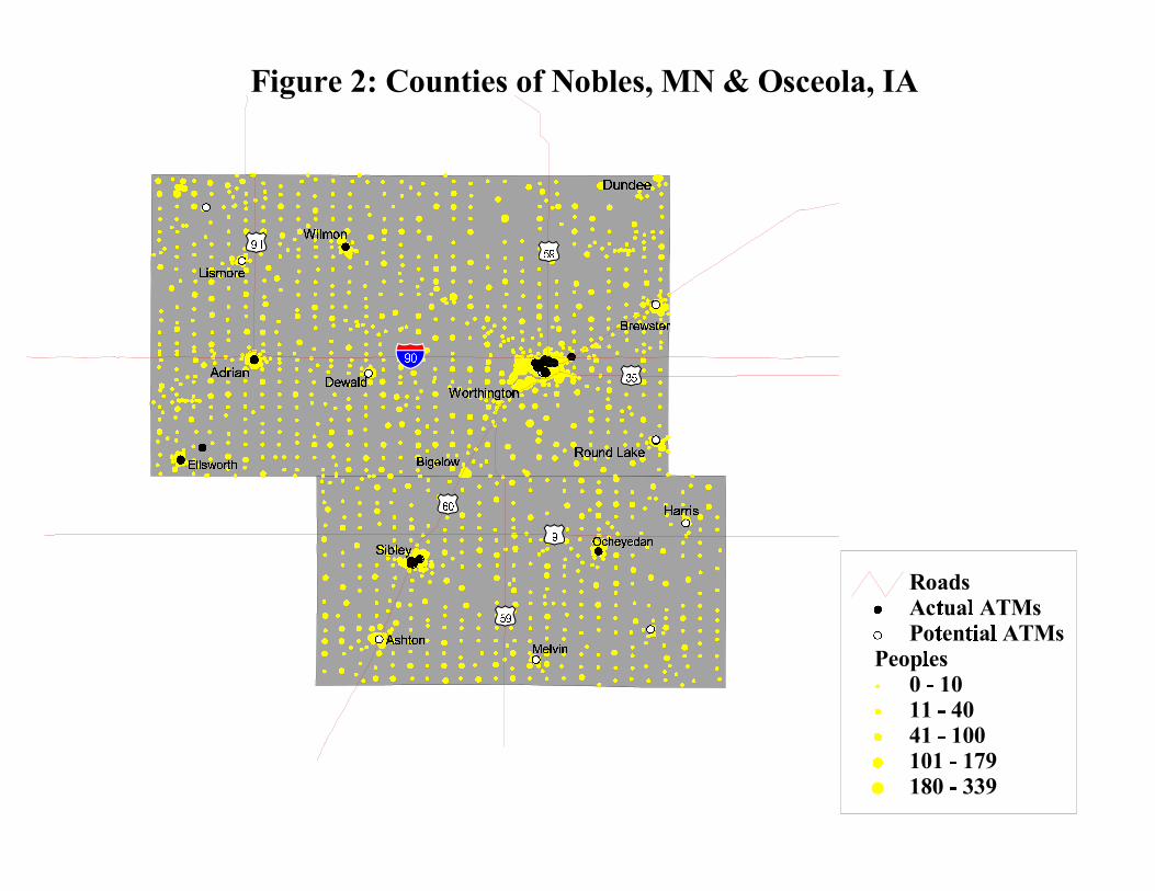
' ( ) * + , -. / / 0 1 2 3 4 5

6 7 8 9 : ; < = >

? @ A B C D

E F G H I J

K L M N O P

Q R S T U V

W X Y Z [ \

] _ a b

c d e f g f h i j

k < l l m n

o

� p

� p

� p

� pp

�� q q r o

� q o